estimating impervious surface in the summer chum esu...
TRANSCRIPT

Estimating Impervious Surface in the Summer Chum ESU under Buildout Conditions 2006 Report Revision: January 2006 In support of Salmon Recovery Planning Submitted to: Scott Brewer Hood Canal Coordinating Council P.O. Box 670 Seabeck, WA 98380-0670 Submitted by: Gretchen Peterson, PetersonGIS 19385 Schooner Court NE Poulsbo, WA 98370 360.697.1170

Estimating Impervious Surface in the Summer Chum ESU under Buildout Conditions
PetersonGIS Contents – 1 1/15/2006
Table of Contents EXECUTIVE SUMMARY ................................................................................................ 1 BACKGROUND ................................................................................................................ 2 MASON COUNTY ............................................................................................................ 2 JEFFERSON, KITSAP, AND CLALLAM COUNTIES ................................................... 4
Methods........................................................................................................................... 4 Input Data........................................................................................................................ 6 Parcel Data Standardization............................................................................................ 7 Zone-code Assignments.................................................................................................. 8 Current Landcode Assignments...................................................................................... 9 Coefficient Calculations................................................................................................ 10 Buildout Landcode Assignments .................................................................................. 11 Buildout Analysis.......................................................................................................... 12
Watersheds................................................................................................................ 13 Riparian Corridors .................................................................................................... 13 Estuaries.................................................................................................................... 15 Nearshore .................................................................................................................. 17
Results........................................................................................................................... 18 Accuracy/Error.............................................................................................................. 46
Input Data.................................................................................................................. 46 Model Implementation.............................................................................................. 46 Measurements of Model Performance ...................................................................... 47
REFERENCES ................................................................................................................. 52 APPENDIX A – Landcode Coefficients........................................................................... 53 APPENDIX B – Buildout Landcode Rules ...................................................................... 54 APPENDIX C – Landcode Conversion Tables ................................................................ 60 APPENDIX D – Landcode Coefficient Histograms......................................................... 69

Estimating Impervious Surface in the Summer Chum ESU under Buildout Conditions
PetersonGIS Contents - 2 1/15/2006
Figures Figure 1 Current impervious surface in Mason County.................................................................................. 3 Figure 2 Buildout analysis process diagram................................................................................................... 5 Figure 3 Impervious Surface Data.................................................................................................................. 6 Figure 4 Buildout database illustration......................................................................................................... 12 Figure 5 Example of riparian corridor delineation, parcel clipping, and IP statistics................................... 14 Figure 6 Hama Hama estuary delineation ................................................................................................... 16 Figure 7 The Duckabush River impact area. ............................................................................................... 16 Figure 8 Kitsap County watershed results .................................................................................................... 20 Figure 9 Jefferson County watershed results................................................................................................ 21 Figure 10 Jimmycomelately Creek buildout statistics .................................................................................. 22 Figure 11 Mason County buildout statistics ................................................................................................. 22 Figure 12 Kitsap County buildout statistics.................................................................................................. 23 Figure 13 Jefferson County buildout statistics ............................................................................................. 24 Figure 14 Watershed numbers referenced in Table 6 ................................................................................... 30 Figure 15 Big Anderson Creek estuary results ............................................................................................. 31 Figure 16 Big Beef Creek estuary results ..................................................................................................... 32 Figure 17 Chimacum Creek estuary results.................................................................................................. 32 Figure 18 Dosewallips River estuary results ................................................................................................ 33 Figure 19 Duckabush River estuary results .................................................................................................. 33 Figure 20 Fulton Creek estuary results......................................................................................................... 34 Figure 21 Jimmycomelately Creek estuary results ....................................................................................... 34 Figure 22 Little Anderson Creek estuary results .......................................................................................... 35 Figure 23 Quilcene estuary results ............................................................................................................... 35 Figure 24 Salmon and Snow Creeks estuary results..................................................................................... 36 Figure 25 Big Anderson Creek riparian corridor results .............................................................................. 38 Figure 26 Big Beef Creek riparian corridor results ...................................................................................... 38 Figure 27 Little Anderson Creek riparian corridor results............................................................................ 39 Figure 28 Salmon and Snow Creeks: riparian results................................................................................... 39 Figure 29 Big Quilcene River riparian corridor results ................................................................................ 40 Figure 30 Little Quilcene River riparian corridor results ............................................................................. 40 Figure 31 Chimacum Creek riparian corridor results ................................................................................... 41 Figure 32 Fulton Creek riparian corridor results .......................................................................................... 41 Figure 33 Duckabush River riparian corridor results ................................................................................... 42 Figure 34 Dosewallips River riparian corridor results.................................................................................. 42 Figure 35 Jimmycomelately Creek riparian corridor results ........................................................................ 43 Figure 36 Nearshore results – modeled current statistics ............................................................................. 44 Figure 37 Nearshore results – buildout statistics .......................................................................................... 45 Figure 38 Scatterplot of actual impervious values versus modeled current.................................................. 47 Figure 39 Standard deviations for landcode IP areas ................................................................................... 49 Figure 40 Distribution of parcels according to histogram interpretation...................................................... 51 Tables Table 1 Data Sources...................................................................................................................................... 7 Table 2 Residential Landcode Assignments................................................................................................. 10 Table 3 Number of units within each IP category under modeled current conditions.................................. 18 Table 4 Number of units within each IP category under buildout conditions .............................................. 18 Table 5 Average IP for all entities within each unit type ............................................................................. 19 Table 6 Watershed level buildout statistics .................................................................................................. 25 Table 7 Estuary results ................................................................................................................................. 31 Table 8 Riparian corridor results .................................................................................................................. 37 Table 9 Histogram analysis .......................................................................................................................... 50
Estimating Impervious Surface in the Summer Chum ESU under Buildout Conditions
PetersonGIS 1 1/15/2006
EXECUTIVE SUMMARY OBJECTIVEE Estimate the increase in impervious SSTUDY AREAA Hood surface (IP) expected if the study area were built out Canal/Eastern Strait of Juan -as allowed under current regulations. de Fuca Summer Chum ESU ANALYSESS 1) Mason County – simplified population increase analysis 2) Clallam, Jefferson, and Kitsap Counties – detailed parcel analysis METHODSS 1) Used OFM (Office of Financial Management) population prediction to determine approximate increase in housing units expected; used average lot size and associated average IP for that lot size to determine corresponding increase in IP. 2) Separated parcels into groups; calculated average IP in each group; assigned those same groups to the parcels under a buildout scenario using zoning and other regulatory information; calculated the change in IP in each parcel from its current group designation to its buildout group designation; quantified this change as it occurred in different unit types applicable to summer chum: watersheds, riparian corridors, estuaries, and nearshore. RESULTSS 1) The estimated IP increase within the Mason County portion of the summer chum ESU is 17% between 2004 and 2025. This estimated IP increase accounts for residential changes only and does not include infrastructure, commercial, and industrial changes to the landscape that may occur. 2) For each unit type as a whole, the estimated IP increases are: watersheds (as measured by the total IP increase in all the parcels) – 29%, or an increase from 11,373 acres to 14,659 acres of IP; riparian corridors – 50% IP increase; estuaries – 50% IP increase; nearshore – 19% IP increase. The average IP within each unit is: Unit Area Average Modeled Current IP Average Buildout IP Watershed* 5.20% 6.19% Riparian Corridor 5.46% 7.79% Estuary 4.10% 6.30% Nearshore 10.90% 13.93%
* only includes watersheds with full parcel data

Estimating Impervious Surface in the Summer Chum ESU under Buildout Conditions
PetersonGIS 2 1/15/2006
BACKGROUND This buildout analysis was designed to gain an understanding of how existing zoning regulations could affect the amount of impervious surface (IP) in the watersheds, riparian corridors, estuaries, and nearshore of the Hood Canal summer chum salmon evolutionarily significant unit (ESU). The work was commissioned by the Hood Canal Coordinating Council (HCCC) for use in the development of the Hood Canal/Eastern Strait of Juan de Fuca Summer Chum Salmon Recovery Plan (The Plan). Two methods of buildout analysis were employed: one in Mason County and the other in Jefferson, Kitsap, and Clallam Counties. In Mason County, a generalized population prediction was used to quantify additional housing units expected and the associated impervious surface increase. A parcel-based approach was used in Jefferson, Kitsap, and Clallam Counties. The parcel approach was a more detailed analysis of how each individual parcel can change under the current regulations.
MASON COUNTY
The current population of Mason County is 50,800 (OFM 2004) and the projected population for the year 2025 is 75,088 (Comp. Plan 2004). To determine the increase in IP expected from the projected addition of 24,288 people to Mason County by the year 2025, a simplified buildout analysis was completed. This approach differs from that in the other counties due to lack of comprehensive parcel and zone data for the county. The average size of a platted lot in Mason County is 3/5 acre (Bob Fink, Planning Manager Mason County, personal communication, March 25, 2005), and this corresponds to the urban low landcode as defined in Table 2. The average impervious surface to land area ratio for parcels with urban low landcodes is 21.14% for parcels in Jefferson and Kitsap Counties as reported in Appendix A. This average was used as a proxy for Mason County, with the assumption that residential parcels in Mason County contain a similar amount of IP as those in neighboring Kitsap and Jefferson Counties. Mason County’s population projection for 2025 translates to an increase of 9,754 housing units for the entire county, given the average household size of 2.49 people per household (U.S. Census Bureau 2000). Using the average size of a platted lot (0.6 acres), this results in the addition of 5,852 parcel acres in the urban low category, for a total of 1,237 acres of additional IP. If it is assumed that the number of new houses is distributed proportionately to the area within the ESU and outside of the ESU, the total IP increase inside the ESU is 606 acres. The present amount of IP within the Mason County portion of the ESU is 3,529 acres (see Figure 1). The estimated IP increase within the Mason County portion of the summer chum ESU, therefore, is 17% between 2004 and 2025 (606acres / 3,529acres). This estimated IP increase accounts for residential changes only and does not include infrastructure, commercial, and industrial changes to the landscape that may occur.

Estimating Impervious Surface in the Summer Chum ESU under Buildout Conditions
PetersonGIS 3 1/15/2006
Figure 1 Current impervious surface in Mason County

Estimating Impervious Surface in the Summer Chum ESU under Buildout Conditions
PetersonGIS 4 1/15/2006
JEFFERSON, KITSAP, AND CLALLAM COUNTIES
Methods The parcel-based approach was developed in order to capture the effect of zoning regulations on each individual tax parcel within the study area. Every parcel’s current landuse, housing density (if any), and zoning allowances and restrictions were considered in order to assign an appropriate buildout IP amount to that parcel. Residential, commercial, and industrial changes to the landscape were all quantified using this methodology. The aggregate of all parcels within the four types of spatial organizing units: watersheds, riparian corridors, estuaries, and nearshore was calculated in order to estimate spatial buildout IP variations. Because the method of determining future buildout potential is derived directly from city and county zoning ordinances, the buildout time horizon is equal to those of the ordinances. Products of this analysis include: • Current parcel landcode • Current parcel IP • Current housing density in select landuses and zones • Modeled buildout parcel landcode • Buildout parcel IP based on estimates derived from current landuses • Maximum buildout parcel IP based on maximum zoning allowances • Summary of buildout estimates for summer chum in each of four unit types:
o Hood Canal watersheds, o summer chum riparian corridors, o summer chum estuaries, and o Hood Canal nearshore
To begin the analysis, parcel layers were standardized and combined. Then, zones were overlayed onto the parcels and each parcel was assigned the appropriate zone code. After than, a system of grouping the parcel’s landuses into appropriate IP categories was developed. The goal was to create groups of parcels that would be expected to contain similar amounts of IP. These groups were termed landcodes (not the same as the landuse codes). The landcodes were used in an overlay with 5-meter IP data to determine the average amount of IP within each landcode. A buildout landcode was assigned to each parcel based on its zone, housing density (if any), current landuse, and current landcode. Using the IP percentages calculated with the current landcode data, the average IP of each landcode was assigned to parcels based on their buildout landcodes. Results were obtained by summing the current IP amount per parcel and summing the buildout IP amount per parcel within each of the four unit types. In addition to those two statistics, the maximum buildout IP amount was assigned to each parcel based on any IP maximums that were specified in the county and city zone codes. In summary, statistics for Hood Canal watersheds, riparian corridors, estuaries, and nearshore were calculated on current IP totals, buildout IP totals, and maximum buildout IP totals. A schematic of this analysis process is presented in Figure 2.

Estimating Impervious Surface in the Summer Chum ESU under Buildout Conditions
PetersonGIS 5 1/15/2006
Figure 2 Buildout analysis process diagram
The analysis followed the assumption that many parcel-types have a potential for an increase in IP. Future changes considered were the further division of rural and open land areas into commercial, industrial, or higher-density residential landuses as well as changes in landuses such as residential to commercial or commercial forest to residential. These were considered likely if the zoning allowed such land division and other factors did not prohibit development (such as sewer requirements). Some landuses were assumed to have negligible future IP changes, such as parks, government facilities, utilities, and government-owned forest lands.
Regulatory Zone layers
Assign zone code(s) to parcels
Modify parcel geometry to obtain
1 parcel per buildable lot
Calculate current housing density for residential parcels
Assign landcodes Landuse / landcode
table
Calculate coefficients: impervious area per landcode /
landcode area
Coefficient table
Calculate buildout density for parcels in residential
zones
Assign buildout landcodes using parcel landcodes,
zones, density, and buildout density
Join with coefficients to
determine buildout IP per parcel
Impervious layer

Estimating Impervious Surface in the Summer Chum ESU under Buildout Conditions
PetersonGIS 6 1/15/2006
Input Data Data relevant to impervious surfaces and zoning regulations within the Hood Canal summer chum ESU were gathered and assessed. Impervious surface (IP) data showing the location of IP versus non-IP lands at a 5-meter resolution were procured from Spatial Sciences and Imaging (see Figure 3). Parcel and zoning layers for Kitsap County, Jefferson County, and Clallam County were obtained. These included sub-areas of Jefferson County but did not include sub-areas of Kitsap County (City of Bremerton) zoning due to non-relevance to summer chum.
Figure 3 Impervious Surface Data The IP data, parcels, and zones were the major layers used in the model. Other supporting data included digital orthophotos, streams, sewers, and aquifers. Summer chum distribution data from the Washington Department of Fish and Wildlife were used to determine upstream extents for the riparian corridor analysis. A few layers were created especially for the model
Estimating Impervious Surface in the Summer Chum ESU under Buildout Conditions
PetersonGIS 7 1/15/2006
and represent composites of pre-existing data. These are the watershed, estuary, and nearshore layers. Table 1 shows the data used and their sources. Table 1 Data Sources Data Source(s) Aerial Imagery Spatial Sciences and Imaging Aquifers Jefferson County Bathymetry Finlayson, University of Washington Driftcells WA Dept. of Ecology Estuaries UW, ESRI, WADNR, PetersonGIS Hydrology WA Dept. of Natural Resources Impervious Surface Spatial Sciences and Imaging Nearshore zones WA Dept. of Ecology, PetersonGIS Parcels Kitsap, Jefferson, and Clallam Counties Sewers Jefferson County Summer chum distribution WA Dept. of Fish and Wildlife Watersheds USGS, Kitsap County, PetersonGIS Zoning Kitsap, Jefferson, and Clallam Counties; City of Port Townsend The zone assignments, housing densities, current landcode and buildout landcode assignments, and other calculations created during the course of the analysis were added to the existing parcel geometry and together make up the buildout database that is referred to in this document.
Parcel Data Standardization Pre-processing of the parcel layers for all three counties was necessary in order to create uniform parcel layers with the desired characteristics. For example, the parcels needed to reflect individually held pieces of land with a single landuse designation (except in Clallam County where multiple landuse designations existed). In some cases parcels were coded with landuses that were not appropriate to this analysis (i.e., a null landuse or exempt code). It was also necessary that parcels not be grouped together, as this would create erroneous population density estimates and zone definitions. The GIS processing details for the Kitsap, Jefferson, and Clallam County parcel layers are expanded upon below. Kitsap County’s parcel layer contained individually held parcels and was mostly coded with landuses consistent with the needs of the analysis. However, there were some parcels that were assigned a landuse of vacant when there was a building on the property (D. Nash, GIS Analyst Kitsap County, personal communication, August 3, 2004). To identify these parcels, all polygons coded as vacant were selected. The applicant field showed 4 with utility applicants, one with a school applicant, and one with a gun club applicant. Because the purpose of identifying each parcel’s landuse was to determine how much impervious surface is, on average, within certain groupings of landuses, it was essential to determine if any of these parcels had impervious surfaces on them so as to not skew the average impervious results for the vacant category. Digital orthophoto analysis determined that no significant imperviousness existed on the utility and school applicant parcels. The gun club parcel did have some existing IP so it was excluded from the vacant landuse IP quantification.

Estimating Impervious Surface in the Summer Chum ESU under Buildout Conditions
PetersonGIS 8 1/15/2006
The Jefferson County parcel layer contained several parcels that were comprised of multiple polygons (J. Miller, personal communication, August 18, 2004). The lines that split these parcels were mostly section lines and are artifacts of the origination of the parcel layer. This situation would have caused the model to overestimate the IP in these parcels. For example, the model would have assigned one house for each polygon (for a total of two) when in fact only one house was allowed within the combined polygons. Another issue was that the parcel layer contained some parcels that were assigned the same parcel identification number (PIN), but were split into separate polygons. It was determined that these were, indeed, individual parcels despite their common PIN. Both issues were resolved within the GIS in order to achieve a one-to-one relationship between a parcel and its polygon. Both the Kitsap and Jefferson County parcel layers were clipped to the summer chum ESU. Some parcel geometry was therefore cut off at the ESU boundary, resulting in a potential for error in that the IP included for those parcels may in fact have been on the non-ESU side of the parcels. However, due to the large number of parcels analyzed, the error involved in the relatively few split parcels is negligible. The modified Kitsap County and Jefferson County parcel layers contained 14,305 and 29,633 parcels, respectively. A subset of the Clallam County parcel layer was used. The parcels lying within the Jimmycomelately watershed and estuary were analyzed for a total of 246 parcels. The Clallam County parcel layer was unique in that an individual parcel could contain one or more landuse codes. The area pertaining to each landuse code was included in the parcel layer. In the pre-processing stage, this was left as-is. A few parcels were originally split into two shapes (i.e., part a and part b) even though they were one parcel. These were combined. In total, 44,184 parcels were analyzed in the buildout analysis.
Zone-code Assignments Once the parcel layers were pre-processed to resolve the coding and delineation anomalies discussed in the previous section, they were overlayed with the zoning layers in order to assign zone codes to each parcel. Most parcels in the study area overlapped with one or more of the zones. The Clallam County parcel layer already contained zone codes and was therefore not a part of this process. The zone-code assignment details for Kitsap and Jefferson Counties are expanded upon below. The most recent zoning layers for Jefferson County, the Port Townsend UGA, the tri-area UGA, and Kitsap County were overlayed onto the parcel layers. A GIS selection process was then performed in order to assign the appropriate zone code to each parcel. In most cases parcels were located within a single zone designation. In cases where a parcel overlapped with multiple zones, the appropriate county or city zone code was consulted to determine how the parcel should be assigned (UDC 2000, PTMC 2003, KCZO 2004). For example, the City of Port Townsend municipal code, chapter 17.12.050, specifies that a parcel of less than one acre is assigned the zone that comprises the majority of the parcel. If a parcel is large enough, the codes may specify that it be split into two or more zones. To accommodate these aberrations, the buildout database was designed to allow up to three zone designations for a single parcel. An exception to the overlay methodology was made for Kitsap County’s right-of-way (ROW) parcels. Even though the ROW parcels overlapped with zone polygons, they were assigned a

Estimating Impervious Surface in the Summer Chum ESU under Buildout Conditions
PetersonGIS 9 1/15/2006
null zone-code. These parcels will likely remain unchanged in buildout regardless of their zone. They were given the buildout landcode of ROW. Some exceptions also occurred in the Jefferson County overlay. First, the rural residential (RR) zone was treated as three separate zones to reflect the three different population density allowances in this category. Second, some of the zone polygons did not have zone codes. These were Olympic National Forest, water, military, and other uncoded areas. These were not assigned zone codes in the buildout database but were assigned the appropriate landcode as described in the next section (e.g., military areas were assigned to the facilities landcode). Finally, four parcels in Jefferson County contained both a zone from the tri-area zoning layer and from the Jefferson County zoning layer. A reference to these parcels could not be located in the tri-area UGA literature. However, the Future Landuse Map splits these parcels where the zones change (FLM 2004). Therefore, for this analysis, the four parcels were split in the same manner.
Current Landcode Assignments All the parcel layers contained landuse codes used by their respective tax assessment offices. The schema used for assigning codes is the same in the three counties. There are hundreds of landuse codes in this schema. For example, the Jefferson County portion of the study area contained 108 unique landuse codes. A smaller grouping of codes was developed for this project since many landuse codes have statistically similar impervious potential. The new grouping schema is referred to in the analysis as landcodes, representing both a grouping of the landuse codes as well as housing density in residential parcels. The landcode grouping built upon similar work conducted by Dave Nash, Kitsap County GIS Analyst, in a previous buildout analysis. The process of assigning landcodes to the parcels involved creating a preliminary grouping schema and calculating housing density in residential parcels. The purpose of the landcode assignments was to create a code schema that could then be applied to the same parcels under buildout conditions and therefore enable a direct comparison between the current landcode and the buildout landcode. The first step in the landcode assignment process was to determine which landuses could be grouped together. The goal was to group landuses with statistically similar IP densities together. Some of the landuses were assigned both current landcodes and buildout landcodes during this step if it was determined that they would remain the same regardless of zoning regulations. For example, in Kitsap County the landuse code 4600 represents parking. The current landcode group it was assigned to was transportation. The buildout landcode was also assigned to transportation since it was unlikely to show an increase in IP regardless of the zone. Other landcodes that remained the same in buildout were: schools, apartments, parks, institutional, utilities, transportation, mobile park, water, rail, streets/highways, church, and hotel/motel. Appendix C contains the landcode conversion tables. The amount of IP in residential landuses can vary depending on the size of the parcels. For example, the Kitsap landuse code 1101 represents one mobile home per parcel. The percentage of IP in the parcel will be much greater for a 5,000 sq ft parcel than for a 5 acre parcel. Therefore, residential landuses were assigned landcodes based on housing density. Housing density was calculated using the number of homes per parcel as specified in the landuse code divided by the area of the parcel (see Table 2). For example, if a parcel

Estimating Impervious Surface in the Summer Chum ESU under Buildout Conditions
PetersonGIS 10 1/15/2006
contains the landuse code for one mobile home and has a calculated housing density of 0.188 (or one housing unit on 5.3 acres), it was assigned a current landcode of rural. Table 2 Residential Landcode Assignments Landcode Density Open Land <= 1 HU1 per 10 acres Rural Between 1 HU per 10 acres and 1 HU per 5.2 acres Estate Between 1 HU per 5.2 acres and 1 HU per 2.6 acres Suburban Between 1 HU per 2.6 acres and 1 HU per 1 acre Urban Low Between 1 HU per 1 acre and 12,480 sq ft Urban Standard
Between 1 HU per 12,480 sq ft and 6,150 sq ft
Urban Medium
Between 1 HU per 6,150 sq ft and 3,114 sq ft
Urban High >= 1 HU per 3,114 sq ft 1 Housing Unit The following landuses presented special cases in Kitsap County: taxtitle, unknown, and null. Most of these were assigned the landcode unbuildable depending on their size. Parcels with these landuses that were less than one acre were given the unbuildable classification. Larger parcels were examined individually using aerial photography to determine their IP amounts, if any. If a parcel appeared to have a building or other source of IP, it was assigned a relevant landcode for the estimated amount of IP. Some special cases existed in Jefferson County as well. One case involved parcels having a landuse of 0. The landcodes for these parcels were determined on an individual basis. For example, four of the parcels with landuse of 0 were on an island not relevant to the study so they were given a landcode of OUT. Another was the existence of two parcels with no landuse codes or descriptions. Digital orthophoto analysis did not reveal enough information. Ultimately, these parcels were assigned residential landcodes, assuming one home on each, due to their proximity to other residential areas. There were less than 50 of these special-case parcels out of 44,184 total parcels analyzed. In Clallam County, many parcels contained multiple landuse codes. Rather than assign multiple landcodes to these parcels, these were consolidated into a single landcode. For example, several large parcels contained a one acre residential landuse such as single family residential while the rest of the parcel was assigned a wooded landuse. However, because zoning usually applied to the entire parcel with the dwelling unit included in zoning restrictions, these parcels were assigned residential landcodes: usually open land or rural depending on the total acreage. Additionally, parcels with landuse codes of 9750, or exempt, were assigned a landcode of vacant, except in one case where the landcode facility was assigned due to IP on that parcel. One parcel was assigned the landcode unbuildable due to not having any landuse codes associated with it.
Coefficient Calculations Once the landcoding process was completed, the IP coefficients were calculated. This process included all the parcels from the Jefferson County and Kitsap County analysis, excluding those from the Clallam analysis, as it was completed at a later date. To determine

Estimating Impervious Surface in the Summer Chum ESU under Buildout Conditions
PetersonGIS 11 1/15/2006
the average IP per landcode, the amount of IP in each landcode was calculated as well as the total area of parcels in each landcode. The total IP was then divided by the total land area for individual landcodes to arrive at average IP percentages per landcode. Results are presented in Appendix A. In order to determine the difference between the estimated IP values calculated in the process described above and the actual IP values, the watershed polygons were used to tally, per watershed, the amount of IP according to the estimated values derived via the landcodes. These were compared to the actual IP in the watershed determined by summing the area of IP in the IP layer when clipped to each watershed. For example, in the Martha John watershed the amount of current IP as derived via the landcode method was 6.96% while the actual IP amount was 4.63%. A comparison of the two values is reported in Table 6 and a scatterplot is shown in Figure 38.
Buildout Landcode Assignments Once the current landcodes were assigned and the coefficients calculated, buildout landcodes were assigned. Many of the parcels retained the same buildout landcode as their current landcode. These were: schools, apartments, parks, institutional, utilities, transportation, mobile park, water, rail, streets/highways, church, and hotel/motel. Additionally, most parcels with the current landcode of wooded were also assigned a buildout landcode of wooded. However, those with a landuse of 8300 – designated timberlands - were assigned residential buildout landcodes due to their location within rural residential zones and the potential for housing development if these lands were sold. Assignment of buildout landcodes for residential zones was based on the current housing densities, potential buildout densities based on the zone regulations, and the current landcode for that parcel. For example, a one acre parcel in a rural residential zone (maximum of one house per 5 acres) that does not yet have a house on it has a current landcode of open land. Even though this parcel is smaller than the required 5 acres, a house can still be built on it since it is already delineated as a separate parcel. Therefore, this parcel would be assigned the buildout landcode urban low because it has the potential to contain a maximum of one house on one acre. The process for assigning buildout landcodes was, for the example noted above: • select all parcels with a current landcode of open land • within that selection, select parcels in rural residential zones (one HU per 5 acres) • for each selected parcel:
o if the parcel area is less than 10 acres, the buildout landcode is assigned based on Table 2, with a buildout of one HU / parcel size
o if the parcel area is greater than or equal to 10 acres, the buildout landcode is assigned based on Table 2 and the buildout of 2 HU / parcel size for parcels less than 15 acres, 3HU / parcel size for parcels less than 20 acres, etc.
Additionally, for all parcels with current landcodes of rural, estate, suburban, urban low, urban standard, urban medium, or urban high, in the rural residential zone (one HU per 5 acres), the parcel is already built-out to the maximum allowed. Therefore the buildout landcode would be equal to the current landcode. An example of the current landcode assignments as compared with buildout landcode assignments is shown in Figure 4. A large

Estimating Impervious Surface in the Summer Chum ESU under Buildout Conditions
PetersonGIS 12 1/15/2006
number of unique combinations of densities and zones were present in the data. The combinations and their respective buildout landcodes are recorded in Appendix B.
Figure 4 Buildout database illustration with RR zone code (one dwelling unit per 20 acres)
Buildout Analysis Parcel buildout IP percentages were calculated using the buildout landcodes assigned in the previous step and the estimated IP percentages calculated from the current landcodes. A one-to-one relationship existed between the buildout landcode database and the current landcode estimated IP table. Current landcodes were also matched with the estimated landcode IP

Estimating Impervious Surface in the Summer Chum ESU under Buildout Conditions
PetersonGIS 13 1/15/2006
table to arrive at an estimated current IP for that parcel. This estimated current IP figure is referred to as “modeled current IP” in the remainder of this report. It is distinct from “actual IP” which is not based on the coefficients, but rather via overlay of the IP layer with the unit being measured. For example, a one acre parcel with a current landcode of rural has a modeled current IP of 3,058 sq. ft. and an estimated buildout IP of 9,209 sq. ft. This is an increase of 6,151 sq. ft. of IP or 201%. Maximum IP calculations were also figured. The zone codes for Jefferson and Kitsap counties contained information concerning the maximum allowable IP in select zones. These maximum IP percentages were assigned to the applicable parcels. The Clallam County zones in the study area did not have maximum IP percentages specified in the Clallam municipal code. Zones that didn’t have specific maximum IP percentages stated in the city and county codes were assigned a maximum IP of 100%. Parcels that remained unchanged in buildout (i.e., current landcode = buildout landcode) were assigned the estimated IP for that landcode, not the maximum IP. Once all of the IP estimates were calculated for both current and buildout landcodes, the parcels were grouped into four unit types: watersheds, riparian corridors, estuaries, and nearshore in order to report on the estimated change of IP within those units.
Watersheds
The difference between current IP and buildout IP in each watershed of the summer chum ESU (excluding Mason County) was calculated in order to illustrate where the zoning regulations and resulting development would have the greatest change if all parcels were built out. A watershed layer was built using existing watershed polygons from Kitsap County, USGS 7th field hydrologic unit codes (HUCs), and 30-meter digital elevation models. Totals for the current and buildout IP estimates were calculated on a per-watershed basis and are shown in Figure 8 and Figure 9. As mentioned earlier, the modeled current IP shown in the maps is calculated by using the coefficients for the current landcodes of each parcel. The actual IP, as determined via overlay of the parcels with the IP data, and the other watershed results are presented in Table 6.
Riparian Corridors
Natal watersheds of both the extant and extinct summer chum salmon populations were analyzed. Riparian corridors were delineated using a 200 foot buffer of the summer chum streams, from the mouth to the upward extent of chum distribution as identified by the Washington Department of Fish and Wildlife. The buildout database was clipped to the corridor polygons and totals for modeled current IP, buildout IP, and maximum buildout IP were calculated (see Table 8 for results and Figure 5 for an example).

Estimating Impervious Surface in the Summer Chum ESU under Buildout Conditions
PetersonGIS 14 1/15/2006
Figure 5 Example of riparian corridor delineation, parcel clipping, and IP statistics

Estimating Impervious Surface in the Summer Chum ESU under Buildout Conditions
PetersonGIS 15 1/15/2006
Estuaries
In the estuarine analysis, the goal was to determine how the land directly contributing runoff to a major summer chum estuary would likely be changing over time with respect to impervious surfaces. Estuaries often have developments surrounding them and may even have impervious surfaces such as highways and docks over them. In order to capture the effect of the parcels surrounding the estuaries, it was necessary to delineate the estuarine boundaries augmented with parcels that touched those boundaries. Thus, the estuarine analysis began with the delineation of the impact areas (estuary plus surrounding parcels) and ended with the computation of both current and future imperviousness within those impact areas. When this study began, no GIS coverage of estuaries in the study area existed so it was necessary to create them for the project. First, a one mile circular buffer polygon was drawn around the end points of each major summer chum stream. This determined the linear extent up the shoreline that the estuary polygon would encompass. The one exception is the Quilcene impact area, which is a combination of the Little Quilcene and the Big Quilcene linear extent. Next, a 200 foot inland buffer of the shoreline was used in order to capture the land immediately surrounding the estuary. Because there are several shoreline lines, none of which are perfect in all cases, the county boundary shoreline was used when it matched with underlying orthophotos and the inside DNR shoreline was used when it was a more appropriate match. The county shoreline represents the county boundary at a 1:24,000 scale as delineated by the U.S. Census Bureau. The DNR shoreline is close to ordinary high water, according to a note from Helen Berry of WA Department of Natural Resources in the hydrology metadata. Finally, the outer extents of the estuaries were determined using a -3.0 meter contour line from the Puget Sound digital elevation model developed by the University of Washington (Finlayson, 2000). The contour line is relative to the mean sea level datum used by older UGSS data (NGVD29). The resultant estuary polygons (see Figure 6) were subsequently merged with the parcels that were wholly or partially contained within the estuary polygons. These merged polygons became the estuarine impact areas and formed the spatial boundaries for the estuarine results (see Figure 7).

Estimating Impervious Surface in the Summer Chum ESU under Buildout Conditions
PetersonGIS 16 1/15/2006
Figure 6 Hama Hama estuary delineation using a one mile buffer of the stream endpoint, 200 foot inland buffer of the shoreline, and 3.0 meter bathymetric contour.
Figure 7 The Duckabush River impact area (3) is the result of overlaying parcels wholly or partially within the estuary (1) with the estuary itself (2). Current impervious surface quantities were derived via two methods. The first was a simple quantification of the impervious surface area in each impact area by clipping the impervious surface data to each impact area and adding up the total pixel area within each. The shifted IP data was used for Jefferson County and Clallam County impact areas while the original IP data was used for the Mason County and Kitsap County impact areas (see shifted IP data discussion in the Accuracy/Error section). The second quantification method used the current landcode designations, their associated mean impervious percentages, combined with the parcel areas to determine the modeled current imperviousness. Future impervious surface quantities under a buildout scenario were also derived via two methods. The first was an average buildout scenario using the mean impervious
= +
1 2 3

Estimating Impervious Surface in the Summer Chum ESU under Buildout Conditions
PetersonGIS 17 1/15/2006
percentages associated with each parcel’s designated buildout landcode. A parcel’s area, for example, was multiplied by its buildout landcode’s mean imperviousness. A summation of all these calculations per each impact area divided by the total area of the impact area gave the expected future imperviousness per impact area. The second method was derived in order to determine the maximum buildout potential for the impact area using the zoning law’s maximum IP allowable. In this case, the maximum IP percentages associated with each parcel’s designated buildout landcode were multiplied by each parcel’s area, summed, and then divided by the total area of the impact area. The results of that calculation illustrate the maximum allowable imperviousness per impact area. Results are reported in Table 7.
Nearshore Nearshore polygons were created in order to analyze the localized buildout changes that could be expected in those parcels that follow the shoreline. To that end, the shoreline (as defined by the parcel layer) was buffered inland to 300 feet. The parcels were clipped to this 300 foot buffer area and assigned IDs according to which driftcell they were closest to. The total amount of impervious surface under current, buildout, and maximum buildout was summed for all the parcels that made up each driftcell ID. The total area within each driftcell ID was also computed. The percent of current, buildout, and maximum buildout IP was then calculated as a fraction of the total area, using the same process as described in the estuary section above. In order to visualize these results, the parcels were then dissolved by driftcell ID to create nearshore polygons showing the location of each nearshore unit. These nearshore units were subsequently joined to the statistics for visualization. The nearshore units and results are shown in Figure 36 and Figure 37.

Estimating Impervious Surface in the Summer Chum ESU under Buildout Conditions
PetersonGIS 18 1/15/2006
Results The amount of impervious surface was quantified within each of the four unit types (watersheds, riparian corridors, estuaries, and nearshore). A summary of the number of units within each 5% IP category for both modeled current and buildout scenarios are presented in Table 3 and Table 4. For example, there were 5 riparian corridors containing 0-5% IP and 7 riparian corridors containing 5-10% IP under the current modeled conditions. Under buildout conditions, there were 2 riparian corridors containing 0-5% IP, 7 riparian corridors containing 5-10% IP, and 3 riparian corridors containing 10-15% IP. Only those units with complete parcel information are included in these tables. Table 3 Number of units within each IP category under modeled current conditions
Riparian Corridors Estuaries Nearshore Watersheds
< 5% 5 8 18 725-10% 7 2 46 30
10-15% 0 0 55 2215-20% 0 0 16 320-25% 0 0 7 025-30% 0 0 3 030-35% 0 0 0 035-40% 0 0 0 0
Table 4 Number of units within each IP category under buildout conditions
Riparian Corridors Estuaries Nearshore Watersheds
< 5% 2 4 11 625-10% 7 6 34 31
10-15% 3 0 44 2715-20% 0 0 34 420-25% 0 0 10 225-30% 0 0 6 130-35% 0 0 5 035-40% 0 0 1 0
The total IP increase in each of the unit types was calculated to give an overview of the amount of change predicted by the model. The following percentages are based on current IP versus buildout IP and are not normalized by total unit area. The percent IP increase, therefore, is simply:
(buildout IP acres - current modeled IP acres) / current modeled IP acres
All the nearshore units together showed a 19% increase in IP. The riparian corridors showed an increase of 50% IP. Estuaries also showed an increase of 50% IP. The total increase in IP calculated for all the parcel data (i.e., not including the Mason County analysis) was 29% (11,372.28 acres to 14,658.95 acres).

Estimating Impervious Surface in the Summer Chum ESU under Buildout Conditions
PetersonGIS 19 1/15/2006
The average IP within each unit type was calculated to determine how unit types compared with respect to the amount of IP within them (see Table 5). The following percentages are normalized by area because they are averages of all the entities within a given unit type. For example, for the watershed averages, the sum of the modeled current IP percentages for all the watersheds was calculated and then divided by the number of watersheds. Table 5 Average IP for all entities within each unit type
Unit Area Average Modeled Current IP
Average Buildout IP
Watershed* 5.20% 6.19% Riparian Corridor 5.46% 7.79% Estuary 4.10% 6.30% Nearshore 10.90% 13.93%
* only includes watersheds with full parcel data

Estimating Impervious Surface in the Summer Chum ESU under Buildout Conditions
PetersonGIS 20 1/15/2006
Figure 8 Kitsap County watershed results

Estimating Impervious Surface in the Summer Chum ESU under Buildout Conditions
PetersonGIS 21 1/15/2006
Figure 9 Jefferson County watershed results

Estimating Impervious Surface in the Summer Chum ESU under Buildout Conditions
PetersonGIS 22 1/15/2006
Figure 10 Jimmycomelately Creek buildout statistics
Figure 11 Mason County buildout statistics

Estimating Impervious Surface in the Summer Chum ESU under Buildout Conditions
PetersonGIS 23 1/15/2006
Figure 12 Kitsap County buildout statistics

Estimating Impervious Surface in the Summer Chum ESU under Buildout Conditions
PetersonGIS 24 1/15/2006
Figure 13 Jefferson County buildout statistics

Estimating Impervious Surface in the Summer Chum ESU under Buildout Conditions
PetersonGIS 25 1/15/2006
Table 6 Watershed level buildout statistics *Grayed results represent watersheds containing only partial parcel coverage: those that are partially within Mason County or in un-analyzed areas of Clallam County. The gray figures, therefore, under-represent the impervious surface. **NA signifies a complete lack of parcels and/or parcel analysis for the watershed; no modeled current IP was calculated. ***Mason County buildout IP results are based on an increase of 0.2% over the actual IP (see the Mason County section of the report). Watersheds spanning both Mason County and another county contain results representing the total of 0.2% plus the buildout IP estimated for the non-Mason County portion of the watershed plus the actual IP in the Mason County portion of the watershed.
No. WATERSHED NAME ACTUAL
IP
MODELED CURRENT
IP
MODELED BUILDOUT
IP
MAXIMUM BUILDOUT
IP
Kitsap County 1 150349 2.77% 3.53% 3.75% 26.86% 2 150362 2.32% 5.17% 6.17% 44.08% 3 150371 9.02% 11.00% 11.08% 99.81% 4 150372 16.00% 10.88% 10.87% 98.90% 5 150373 7.58% 10.99% 10.98% 99.95% 6 150374 11.83% 10.93% 10.92% 99.06% 7 150375 37.48% 12.33% 12.88% 98.11% 8 Bangor Creek 18.87% 10.16% 11.14% 80.34% 9 Big Anderson 3.03% 1.89% 1.97% 8.95%
10 Big Beef (Lower) 8.73% 6.64% 7.75% 58.31% 11 Big Beef (Upper) 8.74% 6.46% 7.66% 73.68% 12 Big Cedar Creek 2.51% 2.83% 3.28% 42.31% 13 Boyce 5.98% 4.36% 5.79% 61.92% 14 Cattail 5.06% 10.48% 11.08% 97.68% 15 Coulter 4.83% 0.64% 6.68% 4.17% 16 Dogfish (East) 14.50% 9.30% 10.39% 34.55% 17 Fern 2.86% 3.01% 3.35% 24.40% 18 Gamble 6.48% 5.64% 6.64% 45.02% 19 Gorst (South Headwaters) 23.32% 9.32% 14.73% 7.69% 20 Gorst (Upper) 3.44% 5.52% 0.56% 31.98% 21 Grovers 3.28% 9.51% 11.60% 1.79% 22 Harding 6.57% 3.18% 3.21% 45.92% 23 Hawks Hole 5.36% 5.99% 7.10% 26.89% 24 Hudson 1.17% 3.52% 4.15% 36.69% 25 Johnson (Lone Rock) 12.65% 10.02% 11.47% 93.67% 26 Johnson (Poulsbo) 2.84% 12.46% 13.17% 7.23% 27 Jump Off Joe 14.54% 14.69% 16.44% 73.06% 28 Kinman 4.59% 5.55% 6.09% 30.44% 29 Laudine Decouteau 0.37% 1.43% 1.63% 9.61% 30 Lemolo-Klaebel 7.60% 9.69% 10.87% 0.47% 31 Little Anderson 13.29% 9.36% 12.47% 77.73% 32 Little Beef 3.76% 5.95% 7.14% 64.88% 33 Little Boston 2.92% 3.92% 4.32% 55.26% 34 Lost 0.00% 3.10% 2.06% 1.88% 35 Martha John Creek 4.63% 6.96% 8.18% 71.33% 36 Middle 3.06% 8.15% 8.14% 81.46% 37 Nellita 10.88% 5.92% 7.38% 62.97% 38 Sam Snyder 4.67% 5.46% 6.23% 29.23%

Estimating Impervious Surface in the Summer Chum ESU under Buildout Conditions
PetersonGIS 26 1/15/2006
No. WATERSHED NAME ACTUAL
IP
MODELED CURRENT
IP
MODELED BUILDOUT
IP
MAXIMUM BUILDOUT
IP
39 Seabeck 9.40% 6.09% 7.53% 71.34% 40 Springa 4.18% 5.00% 6.12% 33.62% 41 Stavis 4.95% 4.25% 5.07% 66.63% 42 Thomas 6.08% 4.11% 5.04% 28.51% 43 Thompson 0.00% 7.74% 8.16% 1.38% 44 Todhunter 1.09% 2.21% 2.65% 23.88% 45 Unnumbered10 23.16% 10.96% 10.97% 98.15% 46 Unnumbered11 12.81% 10.42% 13.09% 74.73% 47 Unnumbered12 15.80% 14.02% 15.91% 88.81% 48 Unnumbered16 13.29% 12.11% 14.93% 88.64% 49 Unnumbered17 0.35% 1.17% 1.17% 5.50% 50 Unnumbered19 10.68% 10.43% 11.91% 85.29% 51 Unnumbered20 13.96% 9.28% 9.86% 81.66% 52 Unnumbered23 5.20% 2.97% 3.92% 35.24% 53 Unnumbered30 10.02% 4.00% 4.16% 29.29% 54 Unnumbered34 33.39% 19.37% 23.89% 84.11% 55 Unnumbered35 7.07% 4.26% 5.97% 28.41% 56 Unnumbered36 10.72% 10.04% 11.50% 89.55% 57 Unnumbered38 24.81% 11.23% 12.34% 97.66% 58 Unnumbered43 1.66% 8.32% 11.80% 86.11% 59 Unnumbered49 0.36% 1.10% 1.10% 1.97% 60 Unnumbered51 11.54% 11.41% 12.93% 85.48% 61 Unnumbered52 19.42% 12.94% 14.44% 97.05% 62 Unnumbered53 24.53% 16.30% 22.91% 57.43% 63 Unnumbered55 21.61% 14.39% 17.23% 77.74% 64 Unnumbered6 0.76% 2.30% 2.67% 21.08% 65 Unnumbered64 6.48% 4.39% 5.18% 24.52% 66 Unnumbered68 1.78% 5.78% 10.48% 56.53% 67 Unnumbered71 6.77% 3.24% 4.96% 24.06% 68 Unnumbered75 5.49% 7.33% 8.99% 79.09% 69 Unnumbered76 1.94% 3.65% 3.82% 75.75% 70 Unnumbered78 0.74% 1.49% 1.49% 6.01% 71 Wildcat 17.04% 9.80% 12.66% 5.55%
Jefferson County
72 Andrews Creek 1.48% 2.18% 2.38% 7.94% 74 Big Quilcene River Lower 5.35% 5.53% 7.23% 18.05% 75 Big Quilcene River Middle 0.36% 1.28% 1.17% 1.93% 76 Big Quilcene River Upper 0.04% 0.00% 0.00% 0.00% 77 Bolton Peninsula 2.84% 3.06% 4.14% 12.07% 79 Cabin Creek 0.00% 0.00% 0.00% 0.00% 84 Chimacum Creek East Fork 2.65% 3.69% 4.16% 14.61% 85 Chimacum Creek Lower 11.35% 10.30% 15.06% 23.41% 86 Chimacum Creek Middle 2.82% 4.37% 4.87% 15.53% 87 Chimacum Creek Upper 2.12% 3.02% 3.52% 13.61% 88 Cliff/Murhut Creek 0.00% 0.00% 0.00% 0.00% 89 Copper Creek 0.00% 0.00% 0.00% 0.00% 90 Crazy Creek 0.00% 0.00% 0.00% 0.00% 92 Devils Lake 0.83% 2.16% 2.56% 8.21% 93 Discovery Bay East Shore Frontal 5.34% 5.82% 7.44% 19.25% 94 Discovery Bay West Shore Lower 2.09% 2.69% 5.13% 21.36% 95 Discovery Bay West Shore Upper 4.11% 2.64% 4.21% 14.91%

Estimating Impervious Surface in the Summer Chum ESU under Buildout Conditions
PetersonGIS 27 1/15/2006
No. WATERSHED NAME ACTUAL
IP
MODELED CURRENT
IP
MODELED BUILDOUT
IP
MAXIMUM BUILDOUT
IP
97 Donovan Creek 1.90% 2.78% 3.57% 13.75% 98 Dosewallips River Headwaters 0.00% 0.00% 0.00% 0.00% 99 Dosewallips River Lower 1.34% 2.62% 3.22% 11.46%
100 Dosewallips River Middle 0.03% 0.39% 0.53% 1.90% 101 Dosewallips River Upper 0.00% 0.00% 0.00% 0.00% 102 Dosewallips River West Fork 0.00% 0.00% 0.00% 0.00% 103 Duckabush River Headwaters 0.00% 0.00% 0.00% 0.00% 104 Duckabush River Lower 1.09% 1.61% 2.14% 6.84% 105 Duckabush River Middle 0.00% 0.00% 0.00% 0.00% 106 Duckabush River Upper 0.00% 0.00% 0.00% 0.00% 112 Fulton Creek 0.08% 0.45% 0.32% 1.09% 118 Heather/Home Creek 0.00% 0.00% 0.00% 0.00% 119 Hidden/Twin Creek 0.00% 0.00% 0.00% 0.00% 121 Indian Island 11.00% 11.00% 10.99% 10.99% 127 Leland Creek 2.55% 2.83% 3.53% 12.34% 128 Lena Creek 0.00% 0.00% 0.00% 0.00% 129 Little Quilcene Lower 1.47% 1.80% 2.59% 12.22% 131 Marrowstone Island 6.82% 7.34% 9.31% 20.32% 133 Mcdonald Creek 1.29% 3.02% 3.86% 11.84% 134 Milk/Ghoul Creek 0.00% 0.00% 0.00% 0.00% 137 Oak/Mats Mats Bay 4.99% 6.38% 8.68% 19.21% 139 Penny Creek 0.01% 0.87% 0.92% 2.27% 140 Port Ludlow 4.41% 4.48% 6.05% 17.04% 141 Port Townsend Bay 22.59% 17.67% 25.22% 29.66% 142 Quimper Peninsula 7.66% 8.77% 13.65% 23.26% 143 Rocky Brook 0.61% 0.79% 0.82% 1.07% 145 Salmon Creek Lower 0.30% 1.64% 1.98% 11.18% 146 Salmon Creek North 0.11% 0.70% 0.78% 4.01% 150 Silt Creek 0.00% 0.00% 0.00% 0.00% 155 Snow Creek 1.11% 1.67% 1.96% 5.65% 156 Spencer/Marple Creek 1.11% 2.08% 2.39% 6.44% 157 Squamish Harbor 2.47% 3.47% 5.27% 14.26% 158 Still Creek 0.00% 0.00% 0.00% 0.00% 159 Tarboo Creek 2.18% 2.69% 3.01% 11.79% 160 Thorndyke Creek 0.81% 1.16% 1.22% 9.79% 161 Toandos Peninsula East Shore Frontal 1.40% 3.50% 5.17% 13.95% 162 Toandos Peninsula West Shore Frontal 1.75% 2.88% 3.68% 13.18% 163 Townsend Creek 0.17% 0.00% 0.00% 0.00% 165 Tunnel Creek 0.04% 0.03% 0.03% 0.03% 166 Tunnel Creek North Fork 0.00% 0.00% 0.00% 0.00% 167 Tunnel Creek South Fork 0.04% 0.00% 0.00% 0.00% 168 Turner Creek 4.04% 4.23% 5.93% 9.64% 169 Walkers Creek 11.04% 7.56% 9.86% 21.36%
Mason County
170 Big Creek 0.00% NA 0.20% NA 171 Brown Creek 0.00% NA 0.20% NA 172 Cedar Creek 0.00% NA 0.20% NA 173 Church Creek 0.00% NA 0.20% NA 174 Dow Creek 2.69% NA 2.89% NA 175 Dry Creek 0.06% NA 0.26% NA 176 Dewatto 1.99% 0.37% 2.24% 0.37%

Estimating Impervious Surface in the Summer Chum ESU under Buildout Conditions
PetersonGIS 28 1/15/2006
No. WATERSHED NAME ACTUAL
IP
MODELED CURRENT
IP
MODELED BUILDOUT
IP
MAXIMUM BUILDOUT
IP
177 Eagle Creek 0.59% NA 0.79% NA 178 Finch Creek 1.17% NA 1.37% NA 179 Fir Creek 0.03% NA 0.23% NA 180 Flat Creek 0.00% NA 0.20% NA 181 Four Stream 0.00% NA 0.20% NA 182 Frigid Creek 0.00% NA 0.20% NA 183 Hama Hama River Lower 0.12% NA 0.32% NA 184 Hama Hama River Middle 0.00% NA 0.20% NA 185 Hama Hama River Upper 0.00% NA 0.20% NA 186 Jefferson Creek 0.00% NA 0.20% NA 187 Jorsted/Ayock Creek 2.12% NA 2.32% NA 188 Lake Cushman Frontal 1.19% NA 1.39% NA 189 Lebar Creek 0.00% NA 0.20% NA 190 Lilliwaup Creek 0.02% NA 0.22% NA 191 Mctaggert Creek 0.33% NA 0.53% NA 192 Mission 2.25% 0.40% 2.35% 2.43% 193 Pine Creek 0.00% NA 0.20% NA 194 Potlatch Creek 2.54% NA 2.74% NA 195 Purdy Creek 2.90% NA 3.10% NA 196 Rule Creek 0.00% NA 0.20% NA 197 Rendsland 1.57% NA 1.77% NA 198 Schaerer Creek 1.26% 0.71% 1.81% 1.75% 199 Skokomish River North Fork Headwaters 0.00% NA 0.20% NA 200 Skokomish River North Fork Lower 0.02% NA 0.22% NA 201 Skokomish River North Fork Upper 0.00% NA 0.20% NA 202 Skokomish River South Fork Lower 0.20% NA 0.40% NA 203 Skokomish River South Fork Middle 0.00% NA 0.20% NA 204 Skokomish River South Fork Upper 0.00% NA 0.20% NA 205 Skokomish River Valley 1.92% NA 2.12% NA 206 Steel Creek 0.00% NA 0.20% NA 207 Sund/Miller Creek 1.37% NA 1.57% NA 208 Shoreline 0.19% 0.40% 0.57% 3.52% 209 Tahuya 2.72% 0.94% 3.17% 5.22% 210 Union 8.72% 3.99% 8.80% 37.12% 211 Vance Creek 0.15% NA 0.35% NA 212 Waketickeh/Cummings Creek 0.20% NA 0.40% NA 213 Mc2 4.64% NA 4.84% NA 214 Mc1 0.05% NA 0.25% NA
Clallam County
73 Bear Creek 3.96% NA NA NA 78 Bungalow/Skookum Creek 0.02% NA NA NA 80 Cameron Creek 0.00% NA NA NA 81 Canyon Creek 0.18% NA NA NA 82 Caraco Creek 0.01% NA NA NA 83 Cassalery Creek 9.51% NA NA NA 91 Deadfall Creek 0.03% NA NA NA 96 Divide Creek 0.00% NA NA NA
107 Dungeness River Below Canyon Creek 5.78% NA NA NA 108 Dungeness River Below Grey Wolf River 0.11% NA NA NA 109 Dungeness River Lower 9.37% NA NA NA 110 Dungeness River Mouth 8.41% NA NA NA

Estimating Impervious Surface in the Summer Chum ESU under Buildout Conditions
PetersonGIS 29 1/15/2006
No. WATERSHED NAME ACTUAL
IP
MODELED CURRENT
IP
MODELED BUILDOUT
IP
MAXIMUM BUILDOUT
IP
111 Eddy Creek 0.04% NA NA NA 113 Gierin Creek 11.40% NA NA NA 114 Gold Creek 0.00% NA NA NA 115 Grand Creek 0.05% NA NA NA 116 Grey Wolf River Lower 0.01% NA NA NA 117 Grey Wolf River Upper 0.00% NA NA NA 120 Howe Creek 0.00% 0.61% 0.93% 3.97% 122 Jimmy-Come-Lately Creek East Fork 0.00% 0.00% 0.00% 0% 123 Jimmy-Come-Lately Creek Lower 1.49% 0.83% 2.42% 6.44% 124 Jimmy-Come-Lately Creek West Fork 0.53% 0.51% 0.67% 3.73% 125 Johnson Creek 5.24% NA NA NA 130 Little Quilcene Upper 0.05% NA NA NA 132 Matriotti Creek 6.59% NA NA NA 135 Miller Peninsula 4.23% NA NA NA 136 Mueller Creek 0.00% NA NA NA 138 Pats Creek 0.63% NA NA NA 144 Royal Creek 0.00% NA NA NA 147 Salmon Creek Upper 0.00% 0.39% 0.39% 1.94% 148 Sequim Bay East Shore 2.83% 0.03% 0.07% 0.51% 149 Sequim Bay West Shore 4.46% NA NA NA 151 Silver Creek 0.01% NA NA NA 152 Slab Camp Creek 0.01% NA NA NA 153 Sleepy Hollow Creek 0.00% NA NA NA 154 Slide Creek 0.00% NA NA NA 164 Trapper Creek 0.00% 0.05% 0.05% 0.05%

Estimating Impervious Surface in the Summer Chum ESU under Buildout Conditions
PetersonGIS 30 1/15/2006
Figure 14 Watershed numbers referenced in Table 6

Estimating Impervious Surface in the Summer Chum ESU under Buildout Conditions
PetersonGIS 31 1/15/2006
Table 7 Estuary results
Estuary Modeled Current
IPBuildout
IPMaximum
Buildout IP
Percent Increase
from current to buildout
Big Anderson 7.01% 8.70% 45.80% 24.17%Big Beef 3.74% 9.11% 54.85% 143.78%Chimacum 3.04% 3.59% 5.65% 18.11%Dosewallips 3.30% 4.11% 6.42% 24.56%Duckabush 3.97% 5.27% 7.72% 32.74%Fulton 7.26% 9.84% 12.25% 35.53%Jimmycomelately 3.01% 8.61% 29.15% 186.05%Little Anderson 4.49% 6.88% 82.98% 53.20%Quilcene 2.20% 2.89% 7.76% 31.22%Salmon/Snow 2.94% 4.02% 7.11% 36.63%
Figure 15 Big Anderson Creek estuary results

Estimating Impervious Surface in the Summer Chum ESU under Buildout Conditions
PetersonGIS 32 1/15/2006
Figure 16 Big Beef Creek estuary results
Figure 17 Chimacum Creek estuary results

Estimating Impervious Surface in the Summer Chum ESU under Buildout Conditions
PetersonGIS 33 1/15/2006
Figure 18 Dosewallips River estuary results
Figure 19 Duckabush River estuary results

Estimating Impervious Surface in the Summer Chum ESU under Buildout Conditions
PetersonGIS 34 1/15/2006
Figure 20 Fulton Creek estuary results
Figure 21 Jimmycomelately Creek estuary results

Estimating Impervious Surface in the Summer Chum ESU under Buildout Conditions
PetersonGIS 35 1/15/2006
Figure 22 Little Anderson Creek estuary results
Figure 23 Quilcene estuary results

Estimating Impervious Surface in the Summer Chum ESU under Buildout Conditions
PetersonGIS 36 1/15/2006
Figure 24 Salmon and Snow Creeks estuary results

Estimating Impervious Surface in the Summer Chum ESU under Buildout Conditions
PetersonGIS 37 1/15/2006
Table 8 Riparian corridor results
Riparian Corridor Corridor
AreaModeled
Current IP
ModeledCurrent
IP Buildout IPBuildout
IP
Max Buildout
IPMax Buildout
IP
Percent Increase
From Current To Buildout
acres acres acres acresBig Anderson Creek 83.13 1.58 1.90% 1.79 2.16% 15.26 18.36% 13.47%Big Beef Creek 308.07 19.51 6.33% 23.18 7.52% 235.70 76.51% 18.82%Little Anderson Creek 28.02 2.18 7.77% 2.44 8.69% 27.11 96.74% 11.82%Salmon Creek 100 3.48 3.49% 3.62 3.63% 11.63 11.65% 4.09%Big Quilcene River 236 9.81 4.15% 16.42 6.95% 37.85 16.02% 67.37%Little Quicene River 130 11.33 8.69% 15.13 11.62% 30.79 23.63% 33.57%Chimacum Creek 299 19.70 6.59% 37.50 12.55% 56.88 19.03% 90.34%Snow Creek 177 13.70 7.74% 18.08 10.21% 40.49 22.87% 31.94%Fulton Creek 40 2.42 6.03% 2.01* 5.02% 6.61 16.45% -16.74%Duckabush River 114 6.54 5.75% 10.90 9.58% 17.91 15.75% 66.62%Dosewallips River 166 8.11 4.89% 11.66 7.04% 26.44 15.96% 43.79%Jimmycomelately Creek 96.59 2.07 2.14% 8.2 8.49% 50.47 52.25% 296.14%
*More than half of Fulton Creek’s summer chum riparian corridor contains a vacant parcel that builds out to the wooded landcode. Wooded has a lower coefficient than vacant.

Estimating Impervious Surface in the Summer Chum ESU under Buildout Conditions
PetersonGIS 38 1/15/2006
Figure 25 Big Anderson Creek riparian corridor results
Figure 26 Big Beef Creek riparian corridor results

Estimating Impervious Surface in the Summer Chum ESU under Buildout Conditions
PetersonGIS 39 1/15/2006
Figure 27 Little Anderson Creek riparian corridor results
Figure 28 Salmon and Snow Creeks: riparian corridor results

Estimating Impervious Surface in the Summer Chum ESU under Buildout Conditions
PetersonGIS 40 1/15/2006
Figure 29 Big Quilcene River riparian corridor results
Figure 30 Little Quilcene River riparian corridor results

Estimating Impervious Surface in the Summer Chum ESU under Buildout Conditions
PetersonGIS 41 1/15/2006
Figure 31 Chimacum Creek riparian corridor results
Figure 32 Fulton Creek riparian corridor results

Estimating Impervious Surface in the Summer Chum ESU under Buildout Conditions
PetersonGIS 42 1/15/2006
Figure 33 Duckabush River riparian corridor results
Figure 34 Dosewallips River riparian corridor results

Estimating Impervious Surface in the Summer Chum ESU under Buildout Conditions
PetersonGIS 43 1/15/2006
Figure 35 Jimmycomelately Creek riparian corridor results

Estimating Impervious Surface in the Summer Chum ESU under Buildout Conditions
PetersonGIS 44 1/15/2006
Figure 36 Nearshore results – modeled current statistics

Estimating Impervious Surface in the Summer Chum ESU under Buildout Conditions
PetersonGIS 45 1/15/2006
Figure 37 Nearshore results – buildout statistics

Estimating Impervious Surface in the Summer Chum ESU under Buildout Conditions
PetersonGIS 46 1/15/2006
Accuracy/Error
Input Data
Details concerning the accuracy and precision of the input data are enumerated here. Both aerial imagery layers (LandSat and Indian Remote Sensing) were collected in August 2003. The publish date for the Kitsap parcel data was August 2003. Jefferson County parcel data did not have a specific publish date; it was received in August of 2004. The watershed unit boundaries were derived from a variety of sources with corresponding variations in accuracy. Some of the watersheds were delineated from a 30 meter DEM in-house, some were from a similar Kitsap County data layer, and others were 7th field USGS hydrologic unit code boundaries. The Kitsap County Code specifies some accuracy details concerning the Kitsap zoning in chapter 17.200.040. The IP data, which were derived from the Landsat TM (30.0 meter color, bands 1-6) and Indian Remote Sensing (5.8 meter black and white with 6-bit radiometric resolution) imagery, have a 94% accuracy when compared to DOQQs. The positional accuracy for the IP data is +/- 40 feet due to the LandSat image and +/- 5 feet due to pixel location. IP data for the Jefferson County portion of the study area were shifted using a rubber-sheeting technique to better match the IP data to the parcel data (projection differences between the layers account for the original shift). IP data for Kitsap County were in spatial conjunction with the Kitsap parcel layer and therefore were not shifted in that portion of the study area.
Model Implementation
Some over or under representation of IP in the Kitsap County portion of the study area may have occurred. Parcels were clipped to the ESU boundary during the modeling process (while the underlying attributes concerning amount of IP within the parcels were not changed) so some of the estimated IP may have actually occurred outside the ESU boundary. This error may not be significant due to the medium spatial scale of the ESU boundary when compared to the large spatial scale of the parcels. Residential buildout for Port Hadlock in Jefferson County may be underestimated in the analysis. In this area there are parcels that, although they contain the same identification number, may have been platted into multiple lots. Those lots could potentially become separate parcels if the required infrastructure exists (e.g., public water and sewer) or if the County changed current policies to relax minimum land area requirements as specified in the County code (D. Christensen, former Manager Jefferson County Natural Resources Division, personal communication, December 28, 2004).
Estimating Impervious Surface in the Summer Chum ESU under Buildout Conditions
PetersonGIS 47 1/15/2006
Measurements of Model Performance
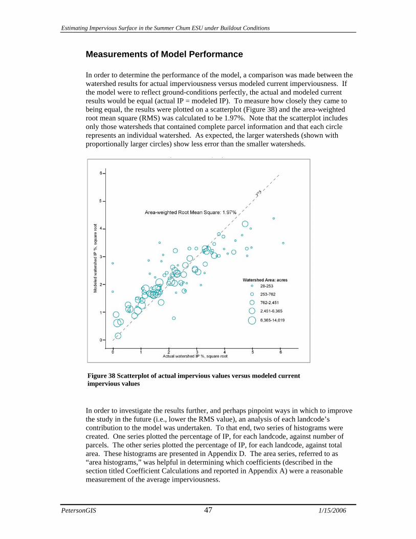
In order to determine the performance of the model, a comparison was made between the watershed results for actual imperviousness versus modeled current imperviousness. If the model were to reflect ground-conditions perfectly, the actual and modeled current results would be equal (actual IP = modeled IP). To measure how closely they came to being equal, the results were plotted on a scatterplot (Figure 38) and the area-weighted root mean square (RMS) was calculated to be 1.97%. Note that the scatterplot includes only those watersheds that contained complete parcel information and that each circle represents an individual watershed. As expected, the larger watersheds (shown with proportionally larger circles) show less error than the smaller watersheds.
Figure 38 Scatterplot of actual impervious values versus modeled current impervious values
In order to investigate the results further, and perhaps pinpoint ways in which to improve the study in the future (i.e., lower the RMS value), an analysis of each landcode’s contribution to the model was undertaken. To that end, two series of histograms were created. One series plotted the percentage of IP, for each landcode, against number of parcels. The other series plotted the percentage of IP, for each landcode, against total area. These histograms are presented in Appendix D. The area series, referred to as “area histograms,” was helpful in determining which coefficients (described in the section titled Coefficient Calculations and reported in Appendix A) were a reasonable measurement of the average imperviousness.

Estimating Impervious Surface in the Summer Chum ESU under Buildout Conditions
PetersonGIS 48 1/15/2006
Visual inspection of the area histograms yielded the following: 22 of the landcodes exhibit sharp peaks, 14 contain a large spread, and 4 are bimodal. These categorizations were further verified by calculating the means (equation 1) and standard deviations (equation 2) of the data once they had been split into 5% intervals, or bins.
∑∑
=
=⋅
= 20
1
20
1
i i
i ii
x
bxμ (Equation 1)
∑∑
=
=−⋅
= 20
1
20
12)(
i i
i ii
x
bx μσ (Equation 2)
Where: μ is the weighted mean (in bin units), ix is the number of acres in a particular bin, b is the bin number, and 20 is the number of bins. The standard deviations were plotted graphically (Figure 39). The standard deviation graph shows, for example, that the vacant landcode’s area histogram has a small spread (i.e., shows a distinctive peak) due to its relatively low standard deviation of 2 bins. That is, 68.26% of the acres designated as vacant contain within plus or minus 10% IP of the mean IP for the vacant landcode (in this case the mean bin was computed as 0.56, which is 2.8% IP). The mean bin value is not to be confused with the coefficient calculated for the landcode, as the coefficients were calculated on the entire layer while the histogram data were grouped into bins, a process by which some precision was lost. However, the relative spread, or confidence, of the coefficients can be approximated in this way.

Estimating Impervious Surface in the Summer Chum ESU under Buildout Conditions
PetersonGIS 49 1/15/2006
0
1
2
3
4
5
6
7
8SA
LT
Auto
/Hig
hway
LAKE OU
T
Phon
e TV
Rad
io
Woo
ded
Airp
orts
Wat
er
Ope
n La
nd
Cem
etar
y
Vaca
nt
Faci
lities
Rur
al
Park
s
RO
W
Park
s Sp
ecia
l
Esta
te
Mob
ile P
ark
Park
s R
esor
ts
Rai
l
Subu
rban
Unb
uild
able
Indu
stria
l Gen
eral
Indu
stria
l Lig
ht
Urb
an L
ow
Min
es
Hot
el/M
otel
Com
mer
cial
Gen
eral
Stre
ets/
Hig
hway
s
Com
mer
cial
Ser
vice
Chu
rch
Indu
stria
l Hea
vy
Scho
ols
Apar
tmen
ts
Urb
an S
tand
ard
Com
mer
cial
Ret
ail
Utili
ties
Gen
eral
Urb
an M
ediu
m
Urb
an H
igh
Tran
spor
tatio
n
Stan
dard
Dev
iatio
n, N
umbe
r of B
ins
Figure 39 Standard deviations for landcode IP areas

Estimating Impervious Surface in the Summer Chum ESU under Buildout Conditions
PetersonGIS 50 1/15/2006
The landcodes categorized as sharp-peaked from the area histograms had standard deviations of less than 3.17 bins. They are: airports, auto/highway, cemetery, estate, facilities, mobile park, open land, parks, parks resorts, parks special, phone TV radio, rail, rural, suburban, unbuildable, vacant, water, wooded, lake, out, ROW, salt. The landcodes categorized as having large-spreads in the area histograms had standard deviations of greater than 3.17 bins. They are: apartments, church, commercial general, commercial retail, commercial service, industrial heavy, industrial light, mines, schools, streets/highways, urban high, urban low, urban medium, urban standard. The remaining landcodes were categorized as bimodal in the area histograms due to the existence of two clear peaks and had standard deviations of greater than 3.7 bins. They are: hotel/motel, industrial general, transportation, utilities general. Ideally, all of the landcodes would exhibit sharp peaks in the area histograms, revealing a high correlation between the landcode’s average IP and the frequency that that IP occurs within those parcels. The large-spread histograms could indicate an improper landuse grouping and possibly result in a higher RMS for the model than could be obtained if these spreads were attempted to be remedied. The bimodal histograms show clearly that the parcels within those 4 landcodes could have been more adequately grouped into 8 landcodes. However, because the bimodal landcodes accounted for no more than 1% of the total land area and 2% of the total current IP, the effort to further refine these landcodes was not seen as worth the small difference in RMS they would likely yield.
Table 9 Histogram analysis
Description Number of
LandcodesTotal Area
(acres)Area as Percent
of TotalTotal IP (acres) Percent IP
Sharp Peak 22 267,158 97% 9,060 81%Large Spread 14 7,225 3% 1,876 17%Bimodal 4 831 0% 239 2% An investigation into the 14 landcodes that show a large-spread type histogram offered the following results. Table 9 shows that these landcodes do not account for much of the overall model (3% of the total land area). However, if the percent IP that these landcodes are responsible for is examined, the influence on the model is more prevalent (17% of the total IP). When the parcels containing landcodes corresponding to the 14 large-spread histograms are plotted, it appears that these parcels may be concentrated in certain watersheds (Figure 40). These are the watersheds for which the circles in Figure 38 are further from the y = x line. The corresponding error may be reduced by investigating the causes for the large-spreads in these histograms and then attempting to improve the landcode grouping. The amount of improvement would depend on the overlap between causes and available data.

Estimating Impervious Surface in the Summer Chum ESU under Buildout Conditions
PetersonGIS 51 1/15/2006
Figure 40 Distribution of parcels according to histogram interpretation

Estimating Impervious Surface in the Summer Chum ESU under Buildout Conditions
PetersonGIS 52 1/15/2006
REFERENCES Clallam County Municipal Code. 2002. Title 33. Finlayson D.P., Haugerud R.A., Greenberg, H. and Logsdon, M.G. 2000. Puget Sound Digital
Elevation Model. University of Washington. http://students.washington.edu/dfinlays/pugetsound/
Kitsap County Zoning Ordinance (KCZO). September 27, 2004. Title 17 – Zoning. http://nt2.scbbs.com/cgibin/om_isapi.dll?clientID=314006&infobase=procode-7&softpage=Browse_Frame_Pg
Mason County Comprehensive Plan (Comp. Plan). 2004. Office of Financial Management (OFM), State of Washington. April 2004. Population of Cities,
Towns, and Counties. Personius, M. 2004. Irondale & Port Hadlock UGA Preliminary Buildout Analysis.
http://www.co.jefferson.wa.us/commdevelopment/UGA%20PDFs/MLA04-29/UGA%20Final%20Buildout%20Analysis%20_March%204_.pdf
Port Townsend Municipal Code (PTMC). November 17, 2003. Title 17 – Zoning. http://search.mrsc.org/nxt/gateway.dll/ptwnmc?f=templates&fn=ptwnpage.htm$vid=municodes:PortTownsend
UGA Future Landuse Map (FLM). 2004. Jefferson County Department of Community Development, Washington. http://www.co.jefferson.wa.us/commdevelopment/UGA%20PDFs/Tri-Area_August16_2004_landuse_draft.pdf
Unified Development Code (UDC) for Jefferson County, Washington. December 18, 2000. Appendix B – Port Ludlow Master Planned Resort. http://www.co.jefferson.wa.us/commdevelopment/udc/final/Appendix%20B_Port%20Ludlow%20MPR%20Ordinance%20Revised.pdf
Unified Development Code (UDC) for Jefferson County, Washington. December 18, 2000. Section 3 – Landuse Districts. http://www.co.jefferson.wa.us/commdevelopment/udc/2004/Section%2003_FINAL-Amended%208-2004%20_Web%20Version_.pdf
U.S. Census Bureau. 2000. Persons Per Household.

Estimating Impervious Surface in the Summer Chum ESU under Buildout Conditions
PetersonGIS 53 1/15/2006
APPENDIX A – Landcode Coefficients
Current Landcode Number of
Parcels Impervious Acreage
Parcel Acreage Coefficient1
LAKE 3 1 169 0.72% ROW 67 924 1785 51.79% SALT 1 1 26 4.52% OUT 1 44 300 14.56% Airports 68 212 1372 15.43% Apartments 181 24 60 39.57% Auto highway 1 1 3 24.74% Cemetery 30 4 82 5.50% Church 45 30 97 31.37% Commercial general 14 3 9 30.40% Commercial retail 217 77 215 36.05% Commercial service 235 144 446 32.41% Estate 2813 1067 11444 9.32% Facilities 100 1009 8911 11.33% Hotel motel 27 13 62 21.63% Industrial general 46 171 564 30.40% Industrial heavy 69 124 323 38.42% Industrial light 63 42 356 11.88% Mines 30 99 484 20.42% Mobile park 18 53 552 9.68% Open land 2895 874 20503 4.26% Parks 616 273 4954 5.51% Parks resorts 44 95 974 9.78% Parks special 3 11 35 31.29% Phone TV radio 6 0 647 0.04% Rail 16 11 68 15.77% Rural 981 482 6868 7.02% Schools 49 67 179 37.53% Streets highways 72 22 58 38.73% Suburban 3917 1023 7120 14.36% Transportation 18 7 18 37.47% Unbuildable 57 4 61 7.30% Urban high 229 3 8 31.70% Urban low 7044 792 3747 21.14% Urban medium 438 18 45 39.25% Urban standard 5751 432 1207 35.81% Utilities general 92 50 196 25.75% Vacant 14838 1625 41256 3.94% Water 57 9 721 1.25% Wooded 2800 1338 159309 0.84%
1The coefficients are based on a larger number of significant digits than shown

Estimating Impervious Surface in the Summer Chum ESU under Buildout Conditions
PetersonGIS 54 1/15/2006
APPENDIX B – Buildout Landcode Rules Kitsap County Notes: these are all for cases when the buildout landcode hadn’t already been assigned during the original landcoding process. Maximum buildouts for Kitsap were: 100% in all zones except IND and BP. IND max buildout was 60% and BP was 50%. Not all possible combinations/permutations are presented here because not all possible combinations existed in the study area If zone = RR AND current landcode = mines, unbuildable, industrial_light, commercial_service, industrial_general, OR industrial_heavy THEN buildout landcode = current landcode. If zone = RP (1 HU per 10 acres) AND
• current landcode = mines, rail, commercial_retail, commercial_service, rural, estate, suburban, urban_low, urban_standard, urban_medium, urban_high, industrial_light, OR unbuildable THEN buildout landcode = current landcode.
• current landcode = open land AND o landuse NOT 91100, 91101, OR 91102 THEN buildout landcode = see Table 2 o Landuse = 91100, 91101, OR 91102 THEN buildout landcode = open land
If zone = IND AND
• current landcode = [residential landcode] THEN buildout landcode = industrial heavy • current landcode NOT [residential landcode] THEN buildout landcode = current landcode
If zone = BP (1 instance in study area) AND current landcode = Vacant AND buildout landcode = industrial general If current landcode = ROW (zone = 0) THEN buildout landcode = ROW If zone = LAKE THEN buildout landcode = LAKE If zone = SALT THEN buildout landcode = water If zone = RW (1 HU per 20 acres) AND
• current landcode = mines, rail, commercial_retail, commercial_service, rural, estate, suburban, urban_low, urban_standard, urban_medium, urban_high, industrial_light, OR unbuildable THEN buildout landcode = current landcode.
• current landcode = open_land THEN buildout landcode = see Table 2 If zone = NC AND
• current landcode = commercial_service THEN buildout landcode = commercial_service • current landcode = open_land THEN buildout landcode = commercial_retail • current landcode = urban_low THEN buildout landcode = commercial_retail
If zone = BC AND current landcode = open_land OR estate THEN buildout landcode = industrial general If zone = CITY THEN buildout landcode = CITY (note: City of Bremerton parcels not analyzed for buildout in this phase)

Estimating Impervious Surface in the Summer Chum ESU under Buildout Conditions
PetersonGIS 55 1/15/2006
If zone = T THEN buildout landcode = current landcode If zone = A THEN buildout landcode = airports If zone = FRL (1 HU per 40 acres) THEN buildout landcode = wooded If zone = HTC AND
• IP coefficient for current landcode less than IP coefficient for industrial heavy THEN buildout landcode = industrial_heavy
• IP coefficient for current landcode greater than IP coefficient for industrial heavy THEN buildout landcode = current landcode
If zone = RHTW OR RHTR (2.5 HU per acre) AND
• Current landcode = industrial light, commercial service, OR commercial heavy THEN buildout landcode = current landcode
• Current landcode = [residential landcode] THEN buildout landcode = see Table 2 (all parcel densities were in the urban low buildout category)
If Zone = RL THEN buildout landcode = rural (note only 2 parcels within this zone. Could not find information on this zone so this is a best-guess) If more than 1 zone existed then separate buildout landcodes for each portion of the parcel were assigned as per the above rules and the resultant coefficients multiplied only by the portion of the parcel that contained that zone Jefferson County Note maximum buildout landcodes and coefficients were assigned based on the rules found in the UGA and zoning documentation and are not enumerated here If zone = EPF AND current landcode = airport THEN buildoutlandcode = airport If zone = AL (1 HU per 20 acres) AND current landcode = open land THEN buildout = open_land If zone = RR (1 HU per 5 acres) AND
• Current landcode = estate, suburban, urban_low, urban_standard, urban_medium, urban_high, OR rural THEN buildout landcode = current landcode.
• Current landcode NOT [residential landcode] THEN buildout landcode = current landcode • Current landcode = open land THEN buildout landcode = see Table 2
Note similar process for all other RR zone densities If zone = LI AND
• current landcode = open land THEN buildout landcode = industrial light • current landcode = industrial heavy, industrial_general, or commercial_service THEN buildout
landcode = current landcode
If zone = LI/C AND current landcode = open_land, commercial retail, commercial service, industrial heavy, industrial light, urban low, OR urban standard THEN buildout landcode = commercial service If zone = LI/M AND
• current landcode = open land, industrial heavy, OR rural THEN buildout landcode = industrial heavy
• current landcode = commercial service THEN buildout = commercial service If zone = HI THEN buildout landcode = industrial heavy

Estimating Impervious Surface in the Summer Chum ESU under Buildout Conditions
PetersonGIS 56 1/15/2006
If zone = CF or RF or IF AND
• current landcode = vacant THEN buildout landcode = wooded • current landcode NOT vacant THEN buildout landcode = current landcode
If zone = MPR-SF (4 HU per acre) AND
• current landcode = vacant AND o area < 3500 sq ft THEN buildout landcode = current landcode o area > 5000 sq ft THEN buildout landcode = see Table 2
• current landcode NOT vacant THEN buildout landcode = current landcode • landuse = 8300 THEN buildout landcode = see Table 2
If zone = MPR-SFT (1 HU per 2.5 acres) AND
• current landcode = church THEN buildout landcode = church • current landcode NOT church THEN buildout landcode = see Table 2
If zone = MPR-MF AND
• current landcode = parks OR apartments THEN buildout landcode = current landcode • current landcode NOT parks OR apartments THEN buildout landcode = apartments
If zone = MPR-RC/CF
• current landcode = vacant THEN buildout landcode = urban high • current landcode NOT vacant THEN buildout landcode = current landcode
If zone = MPR-VC AND current landcode = commercial retail, commercial service, OR parks resorts THEN buildout landcode = current landcode If zone = MPR-RA AND current landcode = open land THEN buildout landcode = open land (note: open land buildout assignment due to existing golf courses assumed to remain golf courses in buildout) If zone = MPR-OSR THEN buildout landcode = current landcode If zone = AP AND
• current landcode = vacant THEN buildout landcode = open land • current landcode NOT vacant THEN buildout landcode = current landcode
If zone = CC THEN buildout landcode = commercial retail If zone = EPF THEN buildout landcode =current landcode If zone = GC AND
• current landcode = commercial retail, commercial service, industrial general, OR industrial light THEN buildout landcode = current landcode
• current landcode = vacant OR [residential landcode] THEN buildout landcode = commercial service
If zone = NC AND
• current landcode = [residential landcode] OR vacant THEN buildout landcode = commercial service
• current landcode NOT [residential landcode] OR vacant THEN buildout landcode = current landcode
If zone = PPR AND
• current landcode = vacant THEN buildout landcode = parks • current landcode NOT vacant THEN buildout landcode = current landcode

Estimating Impervious Surface in the Summer Chum ESU under Buildout Conditions
PetersonGIS 57 1/15/2006
If zone = RI AND
• current landcode = industrial heavy THEN buildout landcode = current landcode • current landcode = vacant THEN buildout landcode = open land (note the Jefferson County Code
states that this zone is to allow for the continuation of existing saw-mills and related activities so it is assumed vacant land may be built out somewhat but not to the extent of an industrial heavy landcode. Only one parcel is in RI with current landcode = vacant.)
If zone = RVC AND
• current landcode = [residential landcode] THEN buildout landcode = commercial service • current landcode NOT [residential landcode] THEN buildout landcode = current landcode
Port Townsend Urban Growth Area If zone = c-1 THEN buildout landcode = commercial retail If zone = c-I/MU (16 HU per 40,000 sq ft) THEN buildout landcode = commercial retail (note: buildout not assigned to urban high due to commercial retail having more realistic coefficient for this zone than urban high) If zone = C-II AND
• current landcode = [residential landcode] THEN buildout landcode = commercial service • current landcode NOT [residential landcode] THEN buildout landcode = current landcode
If zone = C-II(H) AND
• current landcode = [residential landcode] THEN buildout landcode = commercial service • current landcode NOT [residential landcode] THEN buildout landcode = current landcode
If zone = C-II/MU AND
• current landcode = commercial retail THEN buildout landcode = commercial retail • current landcode NOT commercial retail THEN buildout landcode = commercial service
If zone = CIII AND
• current landcode = urban standard, urban medium, vacant, OR open land THEN buildout landcode = commercial service
• current landcode NOT urban standard, urban medium, vacant, OR open land THEN buildout landcode = current landcode
If zone = M-C AND current landcode = [residential landcode] OR vacant THEN buildout landcode = industrial general If zone = MII(A) OR MII(B) AND
• current landcode = vacant THEN buildout landcode = parks • current landcode NOT vacant THEN buildout landcode = current landcode
If zone = PI AND current landcode = [residential parcels] THEN buildout landcode = utilities (note: could also be assigned buildout of schools or facilities, but erring on the upward end of the IP coefficients meant assigning these to utilities as it had a higher coefficient than the others) If zone = P/OS AND
• current landcode = vacant THEN buildout landcode = parks • current landcode NOT vacant THEN buildout landcode = current landcode
If zone = P/OS(B) AND
• current landcode = vacant THEN buildout landcode = facilities
Estimating Impervious Surface in the Summer Chum ESU under Buildout Conditions
PetersonGIS 58 1/15/2006
• current landcode NOT vacant THEN buildout landcode = current landcode If zone = RI(SF) 4 HU per 40,000 sq ft) AND current landcode = [residential landcode] THEN buildout landcode = see Table 2 If zone = RII(SF) AND current landcode = [residential landcode] THEN buildout landcode = see Table 2 If zone = RIII(MF) or RIV(MF) THEN buildout landcode = apartments Port Hadlock/Irondale Urban Growth Area If zone = commercial THEN buildout landcode = commercial service If zone = visitor oriented commercial THEN buildout landcode = commercial retail If zone = light industrial THEN buildout landcode = industrial light If zone = public AND
• current landcode = vacant THEN buildout landcode = facilities • current landcode NOT vacant THEN buildout landcode = current landcode
If zone = single family AND current landcode = vacant OR [residential landcode] AND
• parcel within a Critical Aquifer Recharge Area AND NOT within a sewer service area THEN 3.5 HU per acre, see Table 2 for buildout landcode
• parcel not within a Critical Aquifer Recharge Area OR is within a sewer service area THEN 6 HU per acre, see Table 2 for buildout landcode
If zone = multi-family (7-14 HU per acre) AND current landcode = vacant OR [residential landcode] THEN buildout landcode = see Table 2 (note density was calculating using 14 HU per acre) If zone = mf15-24 THEN buildout landcode = apartments If zone = null AND current landcode = wooded THEN buildout landcode = wooded Clallam County Zones in the study area: R2, R5, R20, CEN, CF If zone1 = R20 (5.863 acres) and zone2 = CF (0.244 acres) and current landcode = vacant THEN assume one house added for a density of 1 / 6.24 and buildout = rural (even if density were 1 / 5.9 buildout would still = rural) If zone = CEN THEN buildout = commercial retail (many landuses possible under CEN zone code but commercial retail is a conservative assumption) 4 parcels contained more than one zone where the second zone was less than or equal to 0.244 acres while the overall parcel size was greater than 6 acres. The amount of parcel area in the second zone was negligible for the purposes of this analysis and the buildout landcode was therefore based on the zone1 assignment. 1 parcel totaled 35 acres in landuse = 8800, landcode = wooded and buildout = wooded while 3.75 acres was assigned landcode = vacant and zone = CEN. For the 3.75 acres, the assumption was that buildout = commercial retail while the remaining acreage buildout = wooded. Because only one buildout landcode was assigned per parcel, the buildout landcode was assigned to wooded but the overall IP statistics for both buildout and max buildout were computed manually using the mix of commercial retail and wooded acres.

Estimating Impervious Surface in the Summer Chum ESU under Buildout Conditions
PetersonGIS 59 1/15/2006
If landcode = vacant THEN buildout = residential landcode depending on allowable density If landcode = vacant and zone = 20 and acres < 5 THEN buildout = vacant (minimum lot size is 5 acres for this zone) If landcode = vacant and acres < 1 THEN buildout = vacant

Estimating Impervious Surface in the Summer Chum ESU under Buildout Conditions
PetersonGIS 60 1/15/2006
APPENDIX C – Landcode Conversion Tables Jefferson County:
Landuse Codes Landcode Buildout Landcode
RESIDENTIAL 1100 depends on density 1101 depends on density 1102 depends on density 1104 depends on density 1200 depends on density 1300 apartments apartments 1400 apartments apartments 1500 mobile_park mobile_park 1600 hotel_motel hotel_motel 1700 apartments apartments 1900 depends on density
MANUFACTURING 2000 industrial_general 2400 industrial_heavy 2450 industrial_heavy 2600 industrial_heavy 3200 industrial_light 3262 industrial_light industrial_light 3270 industrial_heavy industrial_heavy 3300 industrial_light industrial_light 3432 industrial_light industrial_light 3443 industrial_heavy
TRANSPORTATION AND UTILITIES 4111 rail rail 4212 transportation transportation 4300 airports 4315 airports 4411 facilities facilities 4590 streets_highways streets_highways 4600 transportation transportation 4711 phone_tv_radio phone_tv_radio 4800 utilities_general utilities_general 4805 utilities_general utilities_general 4833 utilities_general utilities_general 4841 facilities facilities 4854 facilities facilities
TRADE 5000 commercial_retail 5100 commercial_retail 5192 commercial_retail 5200 commercial_retail

Estimating Impervious Surface in the Summer Chum ESU under Buildout Conditions
PetersonGIS 61 1/15/2006
Landuse Codes Landcode Buildout Landcode 5300 commercial_retail 5360 commercial_retail 5370 commercial_retail 5400 commercial_retail 5410 commercial_retail 5500 industrial_heavy 5530 industrial_heavy 5600 commercial_retail 5700 commercial_retail 5800 commercial_retail 5820 commercial_retail 5830 commercial_retail 5900 commercial_retail 5920 commercial_retail 5932 commercial_retail 5969 commercial_retail
SERVICES 6000 commercial_service 6100 commercial_service 6154 commercial_service 6200 commercial_service 6242 cemetary 6300 commercial_service 6375 industrial_light 6400 commercial_service 6500 commercial_service 6513 commercial_service 6600 commercial_service 6700 facilities facilities 6721 facilities facilities 6722 facilities facilities 6730 facilities facilities 6800 schools schools 6813 schools schools 6900 commercial_service 6911 church church
CULTURAL, ENTERTAINMENT, AND RECREATION 7111 facilities facilities 7112 facilities facilities 7119 facilities facilities 7200 commercial_service commercial_service 7221 commercial_service commercial_service 7311 parks_special parks_special 7400 parks parks 7442 parks parks 7500 parks_resorts parks_resorts 7600 parks parks

Estimating Impervious Surface in the Summer Chum ESU under Buildout Conditions
PetersonGIS 62 1/15/2006
Landuse Codes Landcode Buildout Landcode 7610 parks parks 7620 parks parks 7650 parks parks 7670 parks parks 7690 parks parks 7700 parks parks 7900 parks parks
RESOURCE PRODUCTION AND EXTRACTION 8000 open_land 8100 open_land 8110 open_land 8120 open_land 8300 wooded 8400 industrial_light 8543 mines
UNDEVELOPED LAND AND WATER AREAS 8900 wooded 9100 vacant 9300 water water 9600 open_land 9700 wooded wooded 9720 wooded wooded 9725 wooded wooded 9730 wooded wooded 9800 open_land 9903 industrial_heavy industrial_heavy
Kitsap County:
Landcode Buildout Landcode Landuse Codes
RESIDENTIAL 11100 open_land
11101 depends on density
11102 depends on density
11103 depends on density
11104 depends on density
11105 depends on density
11900 open_land
11901 depends on density
11902 depends on density
12101 depends on density
15000 mobile_park mobile_park
15001 mobile_park mobile_park
16001 hotel_motel hotel_motel
16101 hotel_motel hotel_motel
18300 open_land

Estimating Impervious Surface in the Summer Chum ESU under Buildout Conditions
PetersonGIS 63 1/15/2006
Landcode Buildout Landcode 18301 open_land
19800 open_land
19801 depends on density
19802 depends on density
MANUFACTURING 24000 industrial_heavy
24001 industrial_heavy industrial_heavy
39000 industrial_general
39001 industrial_general
39002 industrial_general
39003 industrial_general
TRANSPORTATION AND UTILITIES 41000 rail rail
43015 airports
45000 streets_highways streets_highways
45900 streets_highways streets_highways
47000 phone_tv_radio phone_tv_radio
47001 phone_tv_radio phone_tv_radio
47005 phone_tv_radio phone_tv_radio
48000 utilities_general utilities_general
48300 utilities_general utilities_general
48301 utilities_general utilities_general
48500 facilities facilities
48504 facilities facilities
48900 utilities_general utilities_general
49000 transportation transportation
TRADE 54101 commercial_retail commercial_retail
54103 commercial_retail commercial_retail
54301 commercial_retail commercial_retail
54501 commercial_retail commercial_retail
55902 industrial_heavy industrial_heavy
58201 industrial_heavy industrial_heavy
59001 industrial_heavy
59002 commercial_retail commercial_retail
59004 commercial_retail commercial_retail
SERVICES 61101 commercial_service commercial_service
62400 cemetary cemetary
63001 commercial_service commercial_service
63700 industrial_heavy
63701 industrial_heavy
63703 industrial_heavy industrial_heavy
63704 industrial_heavy
63707 industrial_heavy
63802 industrial_light

Estimating Impervious Surface in the Summer Chum ESU under Buildout Conditions
PetersonGIS 64 1/15/2006
Landcode Buildout Landcode 63804 industrial_light
63806 industrial_light
63809 industrial_light
64101 auto_highway
67000 facilities facilities
67001 facilities facilities
67002 facilities facilities
67003 facilities facilities
68000 schools schools
68001 schools schools
68003 schools schools
69000 commercial_service
69001 commercial_service
69004 commercial_service
69005 commercial_service
69006 commercial_service
69100 church church
69101 church church
CULTURAL, ENTERTAINMENT, AND RECREATION 72001 facilities facilities
74000 parks parks
74001 parks parks
74002 parks parks
74004 parks parks
74400 parks_special parks_special
74403 parks_special parks_special
75013 parks_resort parks_resort
76000 parks parks
76003 parks parks
79000 parks parks
79001 parks parks
RESOURCE PRODUCTION AND EXTRACTION 81002 open_land
82002 industrial_light
83000 open_land
83001 open_land
83002 open_land
83003 open_land
84000 industrial_light
85000 mines
85001 mines
85003 mines
88000 wooded wooded
88001 wooded wooded
88002 wooded wooded
UNDEVELOPED LAND AND WATER AREAS

Estimating Impervious Surface in the Summer Chum ESU under Buildout Conditions
PetersonGIS 65 1/15/2006
Landcode Buildout Landcode 91000 vacant
91001 vacant
91100 open_land open_land
91101 open_land open_land
91102 open_land open_land
92000 wooded wooded
93000 water water
93900 water water
94000 open_land
94001 open_land
94002 open_land
94003 open_land
95000 wooded wooded
95001 wooded wooded
95002 wooded wooded Clallam County: Landuse Codes Landcode Buildout Landcode
RESIDENTIAL 1100 depends on density (1 house) 1110 depends on density (1 house) 1111 depends on density (1 house) 1112 depends on density (1 house) 1113 depends on density (1 house) 1114 depends on density (1 house) 1115 depends on density (1 house) 1116 depends on density (1 house) 1130 depends on density (1 house) 1135 depends on density (1 house) 1150 depends on density (1 house) 1200 depends on density (1 house) 1220 depends on density (1 house) 1230 depends on density (1 house) 1240 depends on density (1 house) 1300 apartments apartments 1400 apartments apartments 1410 apartments apartments 1500 mobile_park mobile_park 1600 hotel_motel hotel_motel 1731 apartments apartments 1734 apartments apartments 1800 apartments apartments 1810 apartments apartments 1900 depends on density 1910 depends on density 1920 depends on density
MANUFACTURING

Estimating Impervious Surface in the Summer Chum ESU under Buildout Conditions
PetersonGIS 66 1/15/2006
Landuse Codes Landcode Buildout Landcode 2293 industrial_heavy 3400 industrial_heavy 3443 industrial_heavy 3449 industrial_heavy 3510 industrial_heavy
TRANSPORTATION AND UTILITIES 4111 rail rail 4500 streets_highways streets_highways 4580 streets_highways streets_highways 4590 streets_highways streets_highways 4600 transportation transportation 4710 utilities_general utilities_general 4749 utilities_general utilities_general 4800 utilities_general utilities_general 4830 utilities_general utilities_general 4833 utilities_general utilities_general 4834 utilities_general utilities_general 4839 utilities_general utilities_general 4843 utilities_general utilities_general
TRADE 5200 commercial_retail 5211 industrial_general 5212 industrial_general 5220 industrial_general 5300 commercial_retail 5360 commercial_retail 5370 commercial_retail 5392 commercial_retail 5400 commercial_retail 5410 commercial_retail 5462 commercial_retail 5499 commercial_retail 5500 industrial_heavy 5511 industrial_heavy 5520 industrial_heavy 5530 industrial_heavy 5535 industrial_heavy 5600 commercial_retail 5690 commercial_retail 5720 commercial_retail 5800 commercial_retail 5805 commercial_retail 5810 commercial_retail 5820 commercial_retail 5900 commercial_retail 5931 commercial_retail 5932 commercial_retail 5941 commercial_retail

Estimating Impervious Surface in the Summer Chum ESU under Buildout Conditions
PetersonGIS 67 1/15/2006
Landuse Codes Landcode Buildout Landcode 5991 commercial_retail 5999 commercial_retail
SERVICES 6100 commercial_service 6111 commercial_service 6152 commercial_service 6153 commercial_service 6200 commercial_service 6214 commercial_service 6220 commercial_service 6231 commercial_service 6241 commercial_service 6242 cemetary 6290 commercial_service 6300 commercial_service 6319 commercial_service 6370 commercial_service 6375 industrial_light 6379 industrial_light 6391 commercial_service 6400 commercial_service 6411 industrial_heavy 6419 industrial_heavy 6500 commercial_service 6510 commercial_service 6511 commercial_service 6512 commercial_service 6513 commercial_service 6517 commercial_service 6519 commercial_service 6520 commercial_service 6593 commercial_service 6599 commercial_service 6611 industrial_light 6621 commercial_service 6623 commercial_service 6629 industrial_light 6722 facilities facilities 6811 commercial_service 6911 church church 6919 commercial_service 6994 commercial_service 6999 commercial_service
CULTURAL, ENTERTAINMENT, AND RECREATION 7112 facilities facilities 7200 commercial_service commercial_service 7219 commercial_service 7417 commercial_service

Estimating Impervious Surface in the Summer Chum ESU under Buildout Conditions
PetersonGIS 68 1/15/2006
Landuse Codes Landcode Buildout Landcode 7422 parks parks 7499 parks parks 7500 parks_resorts parks_resorts 7511 parks_resorts 7516 parks_resorts 7600 parks parks 7650 parks parks 7700 parks parks 7800 open_land open_land
RESOURCE PRODUCTION AND EXTRACTION 8200 commercial_service 8222 commercial_service 8300 wooded 8500 mines 8543 mines 8800 wooded wooded
UNDEVELOPED LAND AND WATER AREAS 8900 wooded 9100 vacant
9120 commercial_retail (for those parcels with a lot of IP), vacant for those with no IP
9130 industrial_light 9350 open_land open_land 9400 open_land 9500 wooded 9600 open_land 9700 wooded wooded 9730 wooded wooded 9750 vacant

Estimating Impervious Surface in the Summer Chum ESU under Buildout Conditions
PetersonGIS 69 1/15/2006
APPENDIX D – Landcode Coefficient Histograms The following histograms plot the percentage of IP, for each landcode, against total area. Format: Landcode
Tota
l are
a: a
cres
Impervious %, upper bin value

Estimating Impervious Surface in the Summer Chum ESU under Buildout Conditions
PetersonGIS 70 1/15/2006
Airports
0
200
400
600
800
1000
1200
14005 10 15 20 25 30 35 40 45 50 55 60 65 70 75 80 85 90 95 100
Apartments
0
2
4
6
8
10
12
5 10 15 20 25 30 35 40 45 50 55 60 65 70 75 80 85 90 95 100
Auto/Highway
0
1
1
2
2
3
3
5 10 15 20 25 30 35 40 45 50 55 60 65 70 75 80 85 90 95 100
Church
0
5
10
15
20
25
5 10 15 20 25 30 35 40 45 50 55 60 65 70 75 80 85 90 95 100
Commercial General
0
1
2
3
4
5
6
5 10 15 20 25 30 35 40 45 50 55 60 65 70 75 80 85 90 95 100
Commercial Retail
05
101520253035404550
5 10 15 20 25 30 35 40 45 50 55 60 65 70 75 80 85 90 95 100
Commercial Service
0
20
40
60
80
100
120
140
160
180
5 10 15 20 25 30 35 40 45 50 55 60 65 70 75 80 85 90 95 100
Cemetery
0
10
20
30
40
50
60
5 10 15 20 25
30 35 40 45 50 55 60 65 70 75 80 85 90 95 100

Estimating Impervious Surface in the Summer Chum ESU under Buildout Conditions
PetersonGIS 71 1/15/2006
Estate
0
1000
2000
3000
4000
5000
6000
5 10 15 20 25 30 35 40 45 50 55 60 65 70 75 80 85 90 95 100
Facilities
0
500
1000
1500
2000
2500
3000
5 10 15 20 25 30 35 40 45 50 55 60 65 70 75 80 85 90 95 100
Hotel/Motel
0
5
10
15
20
25
5 10 15 20 25 30 35 40 45 50 55 60 65 70 75 80 85 90 95 100
Industrial General
0
50
100
150
200
250
300
350
5 10 15 20 25 30 35 40 45 50 55 60 65 70 75 80 85 90 95 100
Industrial Heavy
0
20
40
60
80
100
120
5 10 15 20 25 30 35 40 45 50 55 60 65 70 75 80 85 90 95 100
Industrial Light
0
50
100
150
200
250
300
5 10 15 20 25 30 35 40 45 50 55 60 65 70 75 80 85 90 95 100
Mines
0
50
100
150
200
250
5 10 15 20 25 30 35 40 45 50 55 60 65 70 75 80 85 90 95 100
Mobile Park
050
100150200250300350400450500
5 10 15 20 25 30 35 40 45 50 55 60 65 70 75 80 85 90 95 100

Estimating Impervious Surface in the Summer Chum ESU under Buildout Conditions
PetersonGIS 72 1/15/2006
Open Land
0
2000
4000
6000
8000
10000
12000
14000
16000
18000
5 10 15 20 25 30 35 40 45 50 55 60 65 70 75 80 85 90 95 100
Parks
0
500
1000
1500
2000
2500
3000
3500
5 10 15 20 25 30 35 40 45 50 55 60 65 70 75 80 85 90 95 100
Parks/Resorts
0
100
200
300
400
500
600
5 10 15 20 25 30 35 40 45 50 55 60 65 70 75 80 85 90 95 100
Parks/Special
0
5
10
15
20
25
30
35
5 10 15 20 25 30 35 40 45 50 55 60 65 70 75 80 85 90 95 100
Phone/TV/Radio
0
100
200
300
400
500
600
700
5 10 15 20 25 30 35 40 45 50 55 60 65 70 75 80 85 90 95 100
Rail
0
5
10
15
20
25
30
35
5 10 15 20 25 30 35 40 45 50 55 60 65 70 75 80 85 90 95 100
Rural
0
500
1000
1500
2000
2500
3000
3500
4000
4500
5 10 15 20 25 30 35 40 45 50 55 60 65 70 75 80 85 90 95 100
Schools
0
5
10
15
20
25
30
35
5 10 15 20 25 30 35 40 45 50 55 60 65 70 75 80 85 90 95 100

Estimating Impervious Surface in the Summer Chum ESU under Buildout Conditions
PetersonGIS 73 1/15/2006
Streets/Highways
0
2
4
6
8
10
125 10 15 20 25 30 35 40 45 50 55 60 65 70 75 80 85 90 95 100
Suburban
0
500
1000
1500
2000
2500
5 15 25 35 45 55 65 75 85 95
Transportation
0
1
2
3
4
5
6
7
8
9
5 10 15 20 25 30 35 40 45 50 55 60 65 70 75 80 85 90 95 100
Unbuildable
0
5
10
15
20
25
30
35
40
45
5 10 15 20 25 30 35 40 45 50 55 60 65 70 75 80 85 90 95 100
Urban High
0
1
1
2
2
3
3
4
4
5
5 10 15 20 25 30 35 40 45 50 55 60 65 70 75 80 85 90 95 100
Urban Low
0
200
400
600
800
1000
1200
5 10 15 20 25 30 35 40 45 50 55 60 65 70 75 80 85 90 95 100
Urban Medium
0
2
4
6
8
10
12
14
5 10 15 20 25 30 35 40 45 50 55 60 65 70 75 80 85 90 95 100
Urban Standard
0
50
100
150
200
250
300
5 10 15 20 25 30 35 40 45 50 55 60 65 70 75 80 85 90 95 100
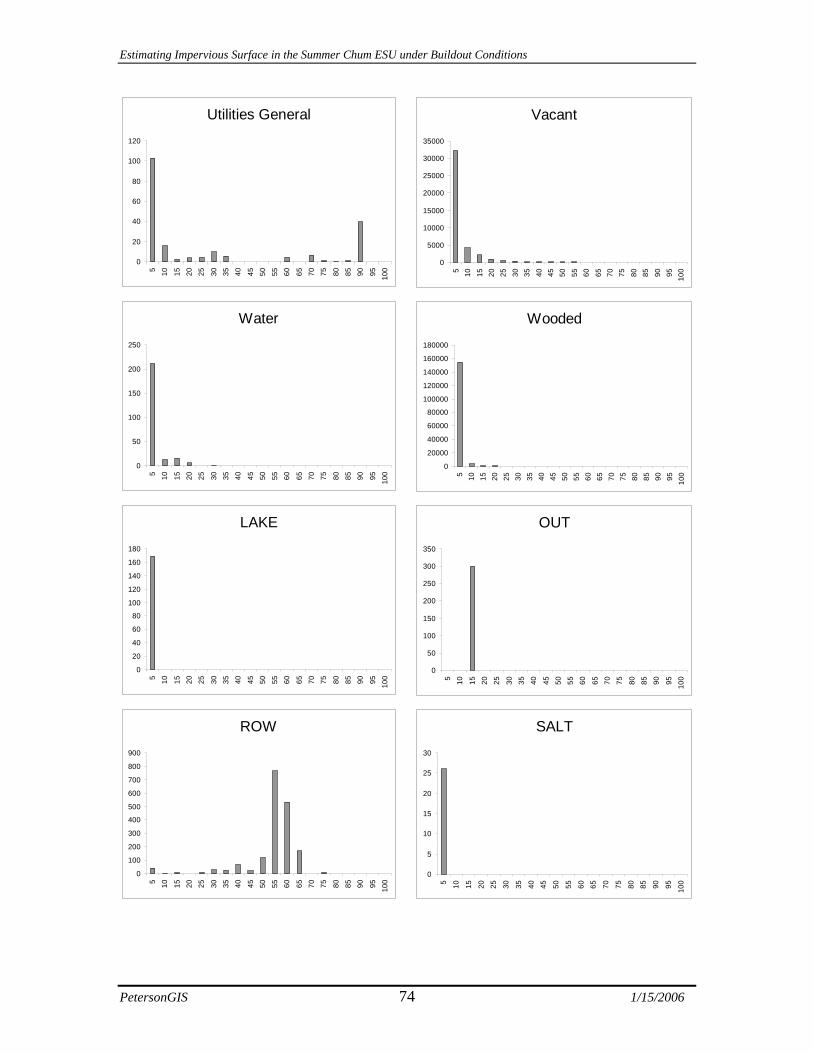
Estimating Impervious Surface in the Summer Chum ESU under Buildout Conditions
PetersonGIS 74 1/15/2006
Utilities General
0
20
40
60
80
100
1205 10 15 20 25 30 35 40 45 50 55 60 65 70 75 80 85 90 95 100
Vacant
0
5000
10000
15000
20000
25000
30000
35000
5 10 15 20 25 30 35 40 45 50 55 60 65 70 75 80 85 90 95 100
Water
0
50
100
150
200
250
5 10 15 20 25 30 35 40 45 50 55 60 65 70 75 80 85 90 95 100
Wooded
0
20000
40000
60000
80000
100000
120000
140000
160000
180000
5 10 15 20 25 30 35 40 45 50 55 60 65 70 75 80 85 90 95 100
LAKE
0
20
40
60
80
100
120
140
160
180
5 10 15 20 25 30 35 40 45 50 55 60 65 70 75 80 85 90 95 100
OUT
0
50
100
150
200
250
300
350
5 10 15 20 25 30 35 40 45 50 55 60 65 70 75 80 85 90 95 100
ROW
0
100
200
300
400
500
600
700
800
900
5 10 15 20 25 30 35 40 45 50 55 60 65 70 75 80 85 90 95 100
SALT
0
5
10
15
20
25
30
5 10 15 20 25 30 35 40 45 50 55 60 65 70 75 80 85 90 95 100

Estimating Impervious Surface in the Summer Chum ESU under Buildout Conditions
PetersonGIS 75 1/15/2006
The next set of histograms plot the percentage of IP, for each landcode, against number of parcels. Format: Landcode
Num
ber o
f Par
cels
Impervious, Parcel Area Ratio

Estimating Impervious Surface in the Summer Chum ESU under Buildout Conditions
PetersonGIS 76 1/15/2006
Airports Commercial Service
Apartments Estate
Cemetery Facilities
Church Hotel / Motel
Commercial General Industrial General
Commercial Retail Industrial Heavy

Estimating Impervious Surface in the Summer Chum ESU under Buildout Conditions
PetersonGIS 77 1/15/2006
Industrial Light Parks: Special
Mines Phone TV Radio
Mobile Park Rail
Open Land Rural
Parks Schools
Parks: Resorts Streets / Highways

Estimating Impervious Surface in the Summer Chum ESU under Buildout Conditions
PetersonGIS 78 1/15/2006
Suburban Urban Standard
Transportation Utilities General
Unbuildable Vacant
Urban High Water
Urban Low Wooded
Urban Medium