estimating hispanic-white wage gaps among women: the
TRANSCRIPT
Upjohn Institute Working Papers Upjohn Research home page
3-1-2015
Estimating Hispanic-White Wage Gaps among Women: The Estimating Hispanic-White Wage Gaps among Women: The
Importance of Controlling for Cost of Living Importance of Controlling for Cost of Living
Peter McHenry College of William and Mary
Melissa McInerney Tufts University
Upjohn Institute working paper ; 15-241
**Published Version**
In Journal of Labor Research 36(3): 249-273 (September 2015).
Follow this and additional works at: https://research.upjohn.org/up_workingpapers
Part of the Labor Economics Commons
Citation Citation McHenry, Peter and Melissa McInerney. 2015. "Estimating Hispanic-White Wage Gaps among Women: The Importance of Controlling for Cost of Living." Upjohn Institute Working Paper 15-241. Kalamazoo, MI: W.E. Upjohn Institute for Employment Research. https://doi.org/10.17848/wp15-241
This title is brought to you by the Upjohn Institute. For more information, please contact [email protected].

Estimating Hispanic-White Wage Gaps among Women:
The Importance of Controlling for Cost of Living
Upjohn Institute Working Paper 15-241
Peter McHenry College of William and Mary E-mail: [email protected]
Melissa McInerney
Tufts University E-mail: [email protected]
March 2015
ABSTRACT
Despite concern regarding labor market discrimination against Hispanics, previously published estimates show that Hispanic women earn higher hourly wages than white women with similar observable characteristics. This estimated wage premium is likely biased upwards because of the omission of an important control variable: cost of living. We show that Hispanic women live in locations (e.g., cities) with higher costs of living than whites. After we account for cost of living, the estimated Hispanic-white wage differential for non-immigrant women falls by approximately two-thirds. As a result, we find no statistically significant difference in wages between Hispanic and white women in the NLSY97. JEL Classification Codes: J31, J70, R23 Key Words: Hispanic-white wage disparities, Cost of living differentials, Immigrant and non-immigrant Hispanics, NLSY Acknowledgments The authors gratefully acknowledge support from a W. E. Upjohn Institute Early Career Research Grant. This research was conducted with restricted access to Bureau of Labor Statistics (BLS) data. The views expressed here do not necessarily reflect the views of the BLS. We thank Alison Courtney and Sarah Gault for excellent research assistance.
1
Estimating Hispanic-White Wage Gaps among Women: The Importance of Controlling for Cost of Living
Peter McHenrya and Melissa McInerneyb
March 2015
Abstract
Despite concern regarding labor market discrimination against Hispanics, previously published estimates show that Hispanic women earn higher hourly wages than white women with similar observable characteristics. This estimated wage premium is likely biased upwards because of the omission of an important control variable: cost of living. We show that Hispanic women live in locations (e.g., cities) with higher costs of living than whites. After we account for cost of living, the estimated Hispanic-white wage differential for non-immigrant women falls by approximately two-thirds. As a result, we find no statistically significant difference in wages between Hispanic and white women in the NLSY97. (JEL codes J31, J70, R23)
The authors gratefully acknowledge support from a W.E. Upjohn Institute Early Career Research Grant. This research was conducted with restricted access to Bureau of Labor Statistics (BLS) data. The views expressed here do not necessarily reflect the views of the BLS. We thank Alison Courtney and Sarah Gault for excellent research assistance. aDepartment of Economics and the Thomas Jefferson Program in Public Policy at the College of William and Mary, Williamsburg, VA, USA. bDepartment of Economics, Tufts University, Medford, MA, USA Email addresses: [email protected] (P. McHenry) and [email protected] (M. McInerney)
2
1. Introduction
Comparisons of Hispanic and non-Hispanic white (hereafter, “white”) labor market
outcomes suggest that Hispanic workers face hurdles in the labor market, relative to white
workers. For example, the median weekly wage of Hispanic workers is only 71 percent of that
earned by whites (United States Department of Labor, 2012), and the Department of Labor’s
Office of Federal Contract Compliance Programs (OFCCP) has increased efforts to recover back
pay for Hispanic workers. Therefore, it is somewhat surprising that several estimates of the
Hispanic-white wage differential among women show a wage premium for Hispanic workers in
specifications that control for observable worker characteristics (e.g., Fryer, 2011—NLSY79
estimates; Neal and Johnson, 1996).1 That is, prior estimates suggest that Hispanic women’s
wages are approximately 15 percent higher than observably similar white women. This premium
likely reflects omitted variables bias, so it is critically important to identify and incorporate this
omitted variable to estimate an accurate wage differential.
To the extent that wages compensate workers for higher local costs of living, it is
important to account for cost of living differences when comparing wages across groups. On
average, Hispanic women live in areas (e.g., cities) with a higher cost of living than whites,
which tends to increase nominal wages of Hispanic women in equilibrium without
correspondingly increasing their purchasing power. The result is that estimates of the Hispanic-
white wage gap that ignore costs of living probably overstate the ability of Hispanic women to
consume out of labor market earnings, relative to white women. In this paper, we provide
1 Other papers find no difference in wages between white and Hispanic women, conditional on observable worker characteristics (e.g., Fryer, 2011—NLSY97 estimates). Recent estimates of the wage gap between Hispanic and white men range from no difference (Fryer, 2007) to a penalty of approximately 0.10 log points (Winters and Hirsch, 2012; Black et al., 2012).

3
updated estimates of wage differentials between Hispanic and white women and show how
important it is to control for cost of living.
Prior work has shown that controlling for cost of living makes a difference in estimates of
Hispanic-white wage gaps among men (Black et al., 2012; Winters and Hirsch, 2012), but has
not considered the role of cost of living in estimates of the wage gap between Hispanic and white
women. It is important to consider women as well, especially since they are such a large part of
the U.S. labor force; women comprise 41 percent of all Hispanic workers and 46 percent of all
white workers (United States Department of Labor, 2012). Further, there are critical policy
implications because existing estimates show a wage premium for Hispanic women. Therefore,
we present wage differentials for women in 2010 and 2011 in two data sets commonly used to
examine wage determination: the National Longitudinal Survey of Youth 1997 (NLSY97) and
the National Longitudinal Survey of Youth 1979 (NLSY79).
We first demonstrate that Hispanic women live in locations (e.g., cities) with
significantly higher average housing costs than whites. Then, in OLS estimates we find that
once we include a control for local cost of living, the difference in conditional wages among
non-immigrant women drops by between 0.06 and 0.11 log points. Among young women ages
27-31 in the NLSY97, we now find no statistically significant difference in wages between
Hispanic and white women. Among mid-career women in the NLSY79, the Hispanic wage
premium drops substantially.
2. Empirical Strategy
The primary innovation of this paper is to examine how estimated wage differentials among
Hispanic and white women change when we account for differences in local cost of living.

4
Location-specific productive features (e.g., the existence of natural resources or the
agglomeration of customers) account for some wage differences across locations. Firms bid up
local land prices in their competition for space in these productive places. Local employers must
compensate workers with higher wages to induce them to live and work where land prices are
high (Moretti, 2011; Roback 1982).2 Below, we show that Hispanics tend to live in areas with
higher costs of living than whites. Therefore, since Hispanics and whites live in different
locations, it will be appropriate to control for local costs of living when estimating ethnic wage
gaps; estimates without a control for cost of living result in Hispanics appearing to perform
better, relative to whites, than estimates that include such a control.
While including explicit controls for cost of living will help us better estimate gaps in
purchasing power between whites and Hispanics, we note that these estimated gaps do not
necessarily measure differences in welfare or utility. Suppose there are local consumption
amenities that increase households’ value of and thereby their demand for local land. The result
would be higher welfare and higher living costs for local residents as long as the supply of local
land is not perfectly price elastic. In the presence of such consumption amenities, our estimates
of the wage gap that take cost of living into account may understate the relative welfare or utility
of people in high-cost, high-amenity locations. Our definition of a location is the Commuting
Zone (e.g., a city), so city-wide consumption amenities (e.g., a well-run local government or
great weather) may cause us to mis-measure ethnic gaps in welfare or utility. However, ethnic
differences in average neighborhood attributes within cities (e.g., a particular school or access to
2 A group of workers with higher wages due to their tendency to locate in places with high firm productivity and high land prices are not better off as a consequence of their high wages than they would be with lower wages and lower costs of living.
5
a park) should not influence the interpretation of our conditional wage gap estimates, which
apply the same cost of living to all residents of a given city (regardless of neighborhood).
To our knowledge, we are the first to include a control for cost of living in estimates of
Hispanic-white wage differentials for women. Both Black et al. (2012) and Winters and Hirsch
(2012) present recent estimates of wage penalties for Hispanic men after including detailed
controls that proxy for cost of living. Black et al. (2012) show that including a control for cost of
living reduces Hispanic performance (i.e., widens the wage penalty), relative to whites, by
between 0.06 and 0.13 log points. Since prior estimates of wage differences between Hispanic
and white women demonstrate that Hispanic women earn a wage premium, including a control
for cost of living is critically important in estimates of wage differences for this group.
We begin by providing updated estimates of the wage gap between Hispanic and white
women in 2010 and 2011. The most recent estimates reflect wage gaps from 2006 (Fryer, 2011),
so updating the estimates will enable us to examine how much our findings may differ because
of the time period studied. Following Fryer (2006), our initial estimation equation is:
𝐿𝑛(𝑤𝑎𝑔𝑒!) = ∝ + 𝛽𝐻𝐼𝑆𝑃𝐴𝑁𝐼𝐶! + 𝛾!𝐴𝐹𝑄𝑇! + 𝛾!𝐴𝐹𝑄𝑇!! + 𝛿!𝑎𝑔𝑒! + 𝛿!𝑎𝑔𝑒!! + 𝜀! (1)
where HISPANICi is an indicator for person i having Hispanic ethnicity, and AFQTi is a score
from a test of cognitive ability. The estimate for β represents the conditional ethnic wage
difference. The AFQT score is a strong predictor of wages and a helpful proxy for a person’s
cognitive ability (Neal and Johnson 1996). The control for AFQTi means that the wage
comparison conditions on pre-market factors that influence workers’ productivity (as in Neal and
Johnson, 1996; Fryer, 2011).3
3 On average, Hispanics have lower AFQT scores than whites, and since there is a wage return to a higher score on the AFQT, omitting the test score results in Hispanics appearing to perform
6
Next, we add a housing cost-based measure of average costs of living where respondents
live (COLi) and control for it in our preferred specifications. Since Hispanics live in areas with a
higher cost of living than whites, we expect that including this measure of cost of living will
reduce the coefficient estimate for β.
We also consider factors that prior research has shown to be important when estimating
racial and ethnic wage gaps among women. First, we address concerns about differential
selection out of work. If Hispanic women with low potential wages are more likely to select out
of work than white women, or white women with high potential wages are more likely to select
out of work than Hispanic women with high potential wages, then estimates that do not address
selection out of work would overstate Hispanic wages, relative to whites. In fact, Duncan, Hotz,
and Trejo (2006) show that Hispanics get less labor market experience than whites, which
suggests that accounting for selection out of work may have an important impact on estimates of
wage differentials. To our knowledge, Winters and Hirsch (2012) is the only study that
examines the role of selection out of work in estimates of Hispanic-white labor market outcomes,
and they estimate differences in annual earnings (not hourly wages) for men, not women. They
find that accounting for selection out of the labor market reduces earnings estimates for
Hispanics, relative to whites, by 0.02 log points (from a -0.13 log points gap to a -0.15 log points
gap). To our knowledge, our estimates are the first to account for selection out of work in
estimates of Hispanic-white disparities for women.
A common approach to address selection is to impute a potential wage for the non-
workers in the sample, and estimate median regressions of wage differentials (e.g., Johnson et
more poorly, relative to whites. Neal and Johnson (1996) find that including a respondent’s AFQT score can boost relative wages for young Hispanic workers, relative to whites, by between 0.11 and 0.14 log points.
7
al., 2000; Chandra, 2003; Neal, 2004; McHenry and McInerney, 2014). We assume that the
imputed wage and the wage an individual could potentially earn (potential wage) fall on the
same side of the conditional median. Under this assumption, wage gap estimates are consistent
for the population median but are not sensitive to the chosen imputed value. We impute low
wages ($1) for non-workers who have low education, a history of government welfare program
use, and no spousal income. We impute high wages ($45) for non-workers who have a high
level of education and are married to high-earning spouses. Details about these imputations are
in the Data section below.
Next, we consider the role of educational attainment. Lang and Manove (2011) show that
controlling for AFQT score in a regression without also including years of education is
appropriate only if, conditional on AFQT, Hispanics and whites attain the same level of
education. In fact, Hispanics in the NLSY79 obtain higher levels of education than whites,
conditional on AFQT scores: Hispanic women with AFQT scores in the middle of the
distribution acquire one additional year of education (Lang and Manove, 2011). Omitting years
of education in estimates that control for AFQT likely overstates how well Hispanics perform
relative to whites. Our preferred specifications also control for respondents’ years of education
(EDUCi), in addition to AFQT scores.
Incorporating these methods, our preferred estimate of the Hispanic-white wage gap is
the estimate for β in:
𝐿𝑛(𝑤𝑎𝑔𝑒!) = ∝ + 𝛽𝐻𝐼𝑆𝑃𝐴𝑁𝐼𝐶! + 𝛾!𝐴𝐹𝑄𝑇! + 𝛾!𝐴𝐹𝑄𝑇!! + 𝛿!𝑎𝑔𝑒! + 𝛿!𝑎𝑔𝑒!! + 𝜙𝐶𝑂𝐿!
+ 𝜆𝐸𝐷𝑈𝐶! + 𝑒! (2)

8
We estimate Equation (2) using OLS and median regression. The observed log hourly wage
among workers is the dependent variable for our OLS estimates. Median regression estimates
also include non-workers with imputed potential wages, as described in detail below.
3. Data
We estimate wage gaps between non-immigrant Hispanic and white women in the 2011 survey
of the NLSY97 and the 2010 survey of the NLSY79.4,5 These longitudinal surveys are
representative of two cohorts of individuals. The NLSY79 is a longitudinal survey of 12,686
individuals that is nationally representative of individuals born between the years 1957 and 1964.
The NLSY97 is a longitudinal survey of 8,984 individuals born between the years 1980 and
1984. NLSY97 respondents are between 26 and 32 years old in 2011 (“early career”), and
NLSY79 respondents are between 45 and 53 years old in 2010 (“mid career”). The NLSY data
include detailed information about hourly wages, labor force participation, educational
attainment, and the respondent’s Armed Forces Qualification Test (AFQT) score. We acquired
the restricted-use files so that we can identify a respondent’s county of residence within the U.S.
(to measure local cost of living).
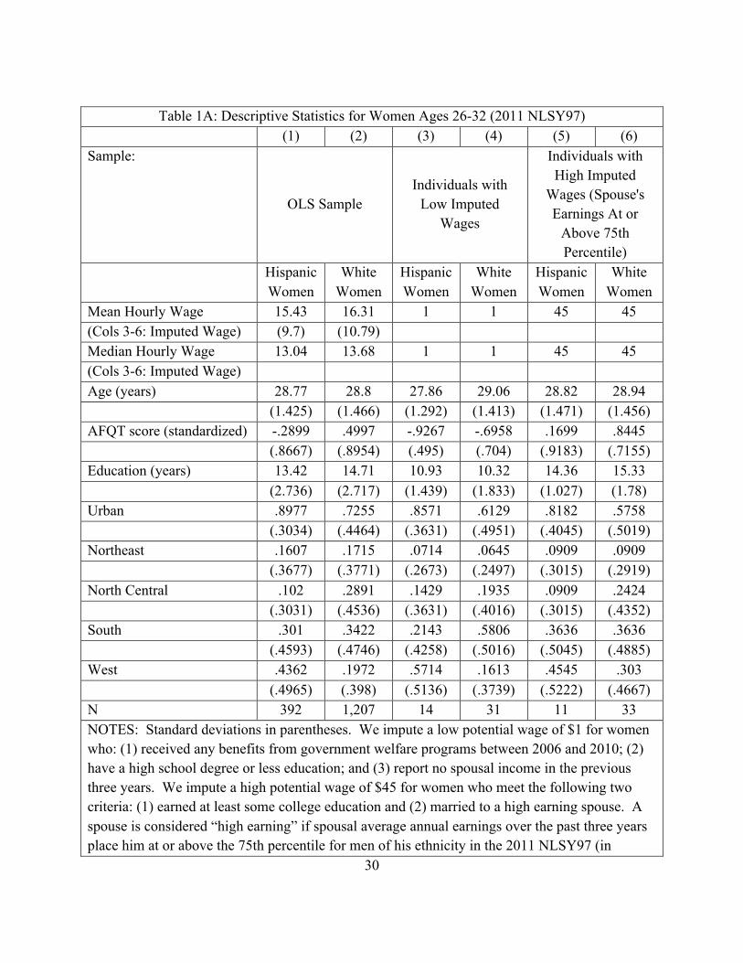
Tables 1A and 1B describe the samples of Hispanic and white respondents we use in our
analysis of wage differences. In Table 1A, columns (1) and (2) present descriptive statistics for
4 The NLSY97 survey is fielded annually, and the NLSY79 is fielded every other year. Therefore, these are the most recent years of data available for each survey. 5 Recent research notes that self-reports of race and ethnicity may be inaccurate due to selective group identification and ethnic attrition (Antman and Duncan, 2014; Duncan and Trejo, 2011). We identify respondent race and ethnicity using as much information from our data sets as we can, including self-reports from multiple surveys (fielded years apart) and assessments made by screeners.

9
the 26 to 32 year old women in the NLSY97 sample.6 We observe that mean and median hourly
wages are higher for white workers than Hispanic workers. Of course, comparing unconditional
means (or medians) does not take labor market skills into account. As shown in rows 4 and 5,
years of education and AFQT scores are greater among whites than Hispanics.7,8
Columns (3) through (6) of Table 1A present descriptive statistics for NLSY97 women
with imputed potential wages. We impute a low potential wage of $1 for those non-working
women who: (1) received any benefits from the Temporary Assistance for Needy Families
(TANF); Women, Infants, and Children (WIC); Food Stamp; or other welfare programs in the
previous five years; (2) have a high school degree or less education; and (3) report no spousal
income in the recent years.9 We adopt these strict criteria to reduce the chance of errors, because
systematically imputing erroneously-low potential wages for women of one ethnic group would
impact our estimate of ethnic wage differences. For example, improperly imputing low potential
wages for white women would result in overstated Hispanic relative wages.
6 To be in the OLS analysis, women must have worked and have valid wage information in 2011, 2010, or 2009. The wage measure we use is the hourly wage at the current or most recent job. If the respondent does not report current wages, we impute the most recent wage from the prior two years (adjusted for inflation by the Consumer Price Index). 7 Our education variable (EDUCi) is the respondent’s years of completed schooling. We start with the highest grade completed that was reported in the most recent survey. We impute a value of 12 for respondents with 11 years of school who ever received a high school diploma or equivalent. We impute a value of 16 for respondents with 15 years of school who ever received a bachelor’s degree. We impute a value of 15 for respondents with more than 15 years of school but no bachelor’s or higher degree. 8 Since schooling and experience influence AFQT scores, our AFQT score variable is standardized by birth year (or equivalently, age when taking the test). We calculate the mean and standard deviation of raw AFQT scores within each birth year cohort. Our AFQT variable is the difference between a respondent’s raw score and the cohort mean, divided by the cohort’s standard deviation. The method follows Neal and Johnson (1996). 9 We identify spouse income for the past five years in the NLSY79 (from the prior three biannual surveys) and the past 3 years in the NLSY97 (from three annual surveys).

10
We impute a high potential wage of $45 for non-working women who meet the following
two criteria: (1) married to a “high-earning spouse” and (2) earned at least some college
education. A “high-earning spouse” has average annual earnings over the past several years that
place him at or above the 75th percentile for men of his ethnic group in the survey (i.e., the 2010
NLSY79 or 2011 NLSY97).10 Improperly imputing high potential wages for Hispanic (but not
white) women would result in overstated Hispanic relative wages. These criteria for imputation
help ensure that the imputed wages are on the same side of the median as the respondent’s
potential wage; however, adhering to these criteria leaves several groups of non-working women
without imputed wages, such as highly educated, persistently unemployed, single women. If our
decision rule leaves more highly skilled white women without an imputed wage than similar
Hispanic women, then we would overstate relative Hispanic wages.11
Women with low imputed wages (columns 3 and 4) have much lower education and
AFQT scores than workers in their own ethnic group, while women with high imputed wages
(columns 5 and 6) have relatively high education levels and AFQT scores. While our imputation
rules imply mechanical education gaps, the differences in AFQT scores between respondents
who have valid wages and respondents with imputed wages (low or high) tend to support our
imputations. The descriptive statistics presented in Table 1B suggest the same patterns hold for
the mid-career women in the NLSY79.
10 We only use the years that a respondent reports nonzero spousal earnings between t-5 and t-1 to identify high earning spouses. For example, a non-working college graduate woman who was single from years t-5 through t-2 would be assigned zero spousal earnings for those years. But if she married a high-earning spouse one year before the survey, then she gets a high imputed wage. 11 We do not impute wages for 160 (204) non-working women in the NLSY97 (NLSY79). 79 (83) of these women had at least some college education. Our main results are robust to changes in imputation. If we impute all missing values as either very high or very low, we obtain similar results to those shown below.
11
3A. Local Cost of Living Control Variable
We are primarily interested in the impact of controlling for local cost of living on
estimates of wage gaps. We first demonstrate that Hispanic and white women face
systematically different costs of living. Figures 1a and 1b illustrate the share of U.S. nationwide
Hispanic and white populations in each county, using the 2010 decennial census. To construct
these shares, we restricted the sample to Hispanic and white women in the same cohorts as the
NLSY97 and NLSY79. These figures show that both Hispanics and whites are concentrated in
large, urban areas (e.g., Los Angeles, Chicago, New York). However, Hispanics are nearly
exclusively located in those large, urban areas, while whites are more likely to live in less
urbanized areas. There are large swaths of the country where less than 0.0001 percent of the
Hispanic population resides in a given county.
For a more explicit measure of differences in the costs of living where Hispanics and
whites live, we construct a local costs index. We measure locations as commuting zones (CZs),
which are collections of counties that have significant economic integration, measured by
journey-to-work links (Tolbert and Sizer, 1996). In metropolitan areas, CZs and metropolitan
statistical areas (MSAs) overlap significantly. The CZ definition provides economically
meaningful boundaries in rural areas, which are often dropped from analyses or pooled together
within a state. Since housing is the most important local price in consumers’ budgets, we
examine differences in housing costs for Hispanic and white respondents. For each CZ, we use

12
the pooled 2009 to 2011 American Community Survey (ACS) to calculate the average gross
monthly rent (including utility costs) for 2 and 3 bedroom dwellings.12
We assign this measure of CZ housing costs to each NLSY respondent based on the CZ
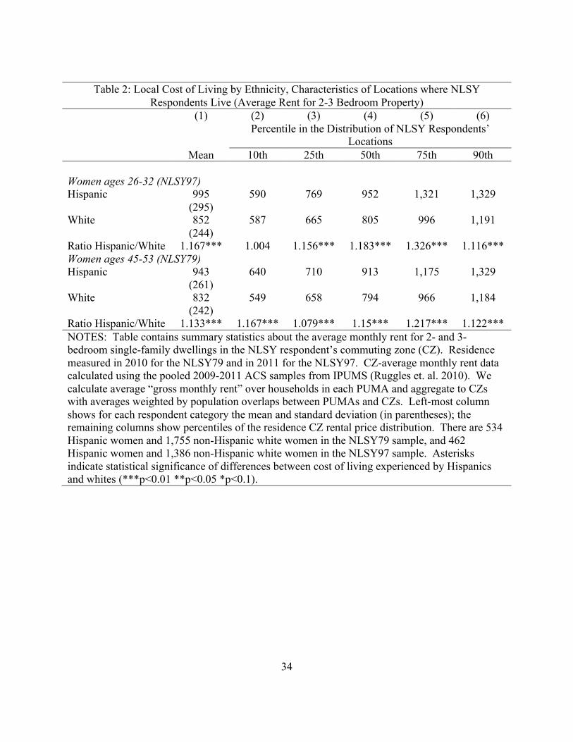
where she lives. Table 2 describes the distributions of average housing costs between Hispanic
and white women’s locations. Column (1) shows Hispanics face higher costs of living on
average: the Hispanic women in our sample face a mean monthly rent of $995 whereas white
women face lower mean monthly rent of $852 (cost of living for the older NLSY79 respondents
shows the same pattern in the bottom panel). This difference is statistically and economically
significant, and the remaining columns of the table show that Hispanics face higher rent at
several quantiles of the cost-of-living distribution. These very large differences imply that it is
important to control for cost of living when comparing earnings between Hispanics and whites.
Otherwise, the comparison will overstate the standard of living that Hispanics can afford with
their earnings.
For the wage regressions, we construct a measure of relative housing costs for each CZ
using the method in McHenry and McInerney (2014).13 We define relative housing costs as the
mean rent in a CZ divided by the average rent over all CZs. We use these relative housing costs
12 The smallest identifiable area in the ACS is the public use microdata area (PUMA), a Census-defined place with population over 100,000. Some PUMA boundaries do not perfectly align with counties. When this is the case, we assign PUMA characteristics to a CZ based on the PUMA’s population share in the CZ (see McHenry, 2014). The housing cost variable is similar to the one in Moretti (2013). 13 Banzhaf and Farooque (2012) compare alternative methods for measuring local housing costs and find that average rental prices perform well: they are closely associated with housing transaction price data (which are more costly to collect), and rental prices are closely associated with measured local amenities and average incomes.

13
to construct a cost of living index that reflects that housing costs comprise only 41 percent of
household expenditures (from the 2011 consumer price index (CPI-U) calculation).14
4. Results
In Table 3, Panel I, we present the coefficient estimate for β from Equation (1). In columns (1)
through (3), we present results for the younger women in the NLSY97. In column (1) we see
that, on average, Hispanic women earn 0.13 log points (13.9 percent) more per hour than white
women with the same AFQT score and of the same age, and median regression estimates yield a
similar result (column (2)). We address selection out of the labor force by imputing wage values
for certain groups of non-working women under the assumption that imputed wages fall either
below or above the conditional median. In column (3), we add 89 women to the sample, 44 with
high imputed wages and 45 with low imputed wages. We find that the conditional wage
premium for Hispanic women rises slightly, from 0.13 log points in column (2) to 0.15 log
points in column (3); however, the two coefficient estimates are not statistically significantly
different than one another.
In Panel II, we now incorporate our main covariate of interest, a control for the cost of
living where respondents live. Figures 1a and 1b and Table 2 showed that Hispanics live in CZs
characterized by higher costs of living, as measured by mean housing rents. We find that
including a control for cost of living eliminates all estimates of a wage premium for Hispanic
14 That is, the CZ housing cost measure is computed as follows: 𝐻𝑜𝑢𝑠𝑖𝑛𝑔𝐶𝑜𝑠𝑡!" =
!"#$%"$&!!( !"#$%"$&!"!
!"!! ) !
and the cost of living is computed as
𝐶𝑜𝑠𝑡𝑜𝑓𝐿𝑖𝑣𝑖𝑛𝑔!" = .4146 ∗ 𝐻𝑜𝑢𝑠𝑖𝑛𝑔𝐶𝑜𝑠𝑡!" + .5854 ∗ 1. The 41.46 percent housing expenditure share in 2011 is from the Bureau of Labor Statistics web page (http://www.bls.gov/cpi/cpiri2011.pdf).

14
women in the NLSY97. None of the coefficient estimates is statistically significant, and the
magnitudes of the coefficients are close to zero, ranging between 0.02 and 0.05 log points. This
suggests that it is critically important to include a measure of costs of living so as not to overstate
Hispanic wages relative to white wages in estimates of ethnic wage gaps.
An alternative way to account for differential costs of living in a wage regression is to
include location-specific fixed effects (see, e.g., Black et al., 2012). In results not shown, we
include a separate intercept for each commuting zone, and we obtain results that are similar to
our results with direct controls for cost of living.15 However, we believe that direct controls for
cost of living are preferable to fixed effects specifications, which partial out all of the variation
across locations, not just variation in local prices.
In Panel III, we consider the role of educational attainment. Lang and Manove (2011)
show that after controlling for AFQT score, Hispanic women in the NLSY79 acquire between
0.72 and 1 additional years of education. If patterns of educational attainment by ethnicity are
similar in the NLSY97, then we would expect that the estimates in Panel II are biased upward.
We first examine patterns of educational attainment by ethnicity, conditional on AFQT score in
the NLSY97 by regressing years of education on an indicator for Hispanic ethnicity, age (and its
square), and AFQT score (and its square). Although we find the coefficient on Hispanic is
positive, it is small and not statistically significant (the coefficient estimate is 0.06 with a
standard error of 0.14).16 Not surprisingly, when we include a control for years of education, the
estimates in Table 3 change very little.17
15 The one exception is that the OLS coefficient estimate for the NLSY97 now achieves statistical significance. 16 The corresponding estimates are somewhat larger in magnitude and achieve statistical significance in the older cohort in the NLSY79: 0.45 with a standard error of 0.12. This suggests

15
In columns (4) through (6), we present analogous results for the mid-career women in the
NLSY79. We notice in Panel I that the estimated wage premium is larger for the older cohort of
women. Using OLS we derive an estimated premium of 0.19 log points for the mid-career
women in the NLSY79, versus 0.13 log points for the younger women in the NLSY97. As for
the younger women, including a control for cost of living in the sample of mid-career women
reduces the Hispanic coefficient estimate by nearly 0.10 log points. However, since the
estimated wage premium in Panel I was so much higher for the mid-career women, we continue
to find a positive and statistically significant wage premium once we include a control for cost of
living, of between 0.09 and 0.13 log points. When we include women with imputed wages, the
coefficient estimate falls to 0.07. Including a control for years of education eliminates the wage
premiums in median regression specifications and further reduces it in OLS estimates.18
Appendix Table A1 compares our preferred Table 3 results to an alternative specification
that replaces the direct cost of living control with indicators for region (South, North Central,
West) and an indicator for living in an urban area. This is a somewhat common approach to
controlling for location (e.g., Antecol and Bedard 2002, 2004). Panel I presents estimates that
that differential patterns in educational attainment by ethnicity have gotten smaller in younger cohorts. 17 In results not shown, we confirm that the addition of cost of living has a similar effect when we instead add a control for years of education to equation (1) first, and a control for cost of living second. That is, adding a control for years of education only reduces the estimated wage premiums by between 0.004 and 0.016 log points, but adding a control for cost of living reduces the estimated wage premium by between 0.074 and 0.125 log points, and the estimate loses statistical significance. 18 In results not shown, we find that the same qualitative conclusions are upheld with a less conservative treatment of selection out of the labor force. For those results, we alternatively impute a low (high) wage of $1 ($45) for all women with missing wages who did not meet our imputation criteria. The only difference is that we now have a statistically significant coefficient estimate (at the 10 percent level) for the NLSY79 median regression results when we impute a low wage of $1 for all women with missing wages (analogous to the column (3) result in Panel III of Table 3).
16
include age, AFQT score, and years of education. Results in Panel II repeat results from the
bottom panel of Table 3 that includes our preferred cost of living measure. In Panel III, instead
of the direct cost of living control, we include an indicator variable for urban residence and
indicator variables for region of the country. Although the coefficient estimates do fall when we
include region and urban status controls, in no case are they sufficient to explain away the
Hispanic wage premium among women that arises after controlling for AFQT score. We believe
this is strong evidence in favor of more detailed location controls (like location fixed effects in
Winters and Hirsch 2012 or Black et al. 2012) or direct measures of cost of living. In fact, as we
show in Appendix Table A2, even after controlling for region and urban residence, Hispanic
women face rental costs that are between 2 and 4 percent higher than whites.
5A. Wage Differences Among Immigrant and Non-Immigrant Hispanics
Hispanics in the U.S. are a heterogeneous group, and prior work has shown how
estimates of wage gaps vary among different subgroups of Hispanics. For example, recent
immigrants might face very different hurdles in the labor market than U.S.-born Hispanics.
Work by Trejo (1997) and Duncan et al. (2006) illustrates the importance of separately
considering labor market outcomes for U.S.-born versus foreign-born Hispanics.19
19 Trejo (1997) examines wage differentials among Mexican and white men and shows labor market returns to education and work experience differ for the newly arrived (i.e., first or second generation) vs. those in the third generation or higher. Further, wage gaps for Mexican American men are over three times larger for first generation Mexican men (relative to first generation white men) than they are for men of the third generation or higher.
17
For two reasons, our preferred estimates in Table 3 exclude NLSY respondents who are
immigrants.20 First, labor market experiences and returns to characteristics like schooling and
age may differ substantially between foreign-born and U.S.-born workers (Duncan, Hotz, and
Trejo, 2006). Second, since individuals are only included in the NLSY data if they were in the
United States in 1997 (for the NLSY97) and 1979 (for the NLSY79), survey respondents in 2011
and 2010 may not be representative of the U.S. immigrant population at that time. In fact,
American Community Survey (ACS) data show that as of 2011, 65 percent of young Hispanic
immigrant women immigrated to the U.S. after 1997, and 73 percent of mid-career Hispanic
immigrant women immigrated to the U.S. after 1979.
In Appendix Table A3, we compare characteristics of the Hispanics in the NLSY surveys
and similarly-aged Hispanic U.S. residents in 2011. In columns (1) and (2), we examine mean
hourly wages and years of educational attainment for Hispanics in the NLSY97 and Hispanics in
the 2011 American Community Survey (ACS). Hispanic immigrants in the NLSY97 report
higher mean wages than their counterparts in the ACS, $15.17 versus $12.38. A similar pattern
is observed for years of education: 12.59 for women in the NLSY97 versus 10.8 for women in
the ACS. What is striking is that even when we restrict attention to Hispanic immigrants in the
ACS who have been in the U.S. since 1997, we still find that Hispanic immigrants in the
NLSY97 have higher mean wages and more years of education, although the differences are
smaller. We infer that the NLSY97 does not include as many low-skilled immigrant Hispanics
as the ACS. In fact, only 59 percent of Hispanic immigrants in the NLSY97 have a high school
degree or less education whereas 64 percent of Hispanic immigrants in the ACS (who were in the
20 In the NLSY97, we exclude 85 immigrants (70 Hispanic, 15 white), and in the NLSY79 we exclude 153 immigrants (122 Hispanic, 31 white).

18
U.S. before 1997) are in this lower education category.21 In columns (3) and (4) we present
differences in hourly wages and years of education for immigrant women ages 46-53 in the
NLSY79 versus the ACS, and the pattern that immigrants in the NLSY79 earn higher wages and
acquire more years of education than similarly-aged immigrants in the ACS is upheld.
Even though Hispanic immigrants in the NLSY surveys are not representative of the
Hispanic immigrant population in 2010 and 2011, results in Table 4 show that our results are not
sensitive to the inclusion of immigrants in the samples. The first row in Table 4 repeats Panel III
from Table 3, which includes cost of living and years of education controls for samples of non-
immigrants. The second row in Table 4 now includes immigrants in the sample, and the
regression specification includes an indicator variable flagging immigrant respondents. Results
for samples that include immigrants are very similar to those that omit immigrants. Although we
now find positive and statistically significant wage premiums in columns (5) and (6), they are not
statistically different than the point estimates presented in the sample of non-immigrants.
5B. Wage Differences Between Mexicans and Whites
Prior work has also shown that average labor market outcomes differ for Hispanics of different
national-origin groups. For example, Mexican American women have lower employment rates
than Puerto Ricans and Cubans (Duncan et al., 2006). Some prior estimates of wage differentials
for men (Trejo, 1997) and women (Antecol and Bedard, 2004) have restricted focus to a more
narrowly-defined group based on country of family origin, such as Mexico. We also present
21 Not only is there a smaller share of Hispanic immigrants in the NLSY97 with lower levels of education, but the less-educated Hispanic immigrants in the NLSY97 have higher mean hourly wages and more years of education. Mean hourly wages in this group are $15.17, versus $11.28 for their counterparts in the ACS. Less-educated Hispanic women in the NLSY97 acquired 11.35 years of education, on average, versus 10.28 among their counterparts in the ACS.
19
separate estimates for Hispanics of Mexican descent both because the samples in the NLSY97
and NLSY79 are sufficiently large to estimate wage differentials for this group and because, as
Trejo (1997) shows, people of Mexican descent have long been among the most economically
disadvantaged in the U.S.
The third row of Table 4 shows results that restrict the Hispanic sample to those of
Mexican descent.22 In addition to providing evidence based on a common country of origin,
these estimates are more directly comparable to prior estimates in the literature (see, e.g.,
Antecol and Bedard 2002). Excluding non-Mexican Hispanics reduces the sample size by
approximately 200 individuals, for both cohorts of women. We continue to find no evidence of a
wage penalty among women in specifications that control for local cost of living (plus education
and quadratics in age and AFQT score). This is striking because prior work examining wage
differentials by Hispanic ethnicity has tended to find wage penalties among Mexican men (see,
e.g., Trejo, 1997; Antecol and Bedard, 2004).
5C. Differences by Educational Attainment
Table 5 shows differences in ethnic wage gap estimates between respondents with more and less
education. We present our preferred specification separately for those with a high school degree
or less (second row) and those with some college (third row). For the younger cohort, there is
little evidence for statistically significant differences in wages. We note that although the OLS
results in column (1) suggest that less educated Hispanic women enjoy a wage premium of
approximately 0.10 log points, we do not see a corresponding premium in estimates that use
22 Respondents of Mexican descent in the NLSY97 are the subset of respondents we previously identified as Hispanic who also selected “Mexican” as their primary ethnicity in the 1999 survey.
20
median regression. This suggests that the premium observed in column (1) is driven by a few
outliers. We also note that we find no evidence of wage differentials among young women with
at least some college. In contrast, the results for the mid-career women suggest a different
pattern: the estimated wage premiums appear to be driven by higher educated women. We
observe a wage premium of between 0.12 and 0.15 log points for mid-career Hispanic women
with at least some college education. This is consistent with some earlier work that found black
wage premiums (relative to whites) among highly educated women (see, e.g., Black et al., 2008;
Fisher and Houseworth, 2011).
5D. Role of Actual Labor Market Experience
Since differences in actual labor market experience may arise due to discrimination in hiring and
retention, specifications that do not control for actual experience incorporate a potentially fuller
picture of labor market discrimination and differential opportunities across groups (as in our
preferred estimates in Table 3). As shown in Duncan et al. (2006), Hispanics have fewer years
of actual labor market experience than whites. Therefore, comparing white and Hispanic
individuals with the same potential experience would tend to understate the human capital white
workers have developed. We expect that estimates of Hispanic-white wage differences that only
include controls for a worker’s age or potential experience would result in Hispanics appearing
to earn lower wages, relative to whites. Antecol and Bedard (2002) show that length of work
experience accounts for approximately half of the Hispanic-white wage gap among women. For
comparability to the prior literature, and to quantify the return to an hour of work for workers
with similar human capital, we also present estimates that include a control for actual labor
market experience. In the last row of Table 5, we find that, relative to our baseline estimates, the

21
coefficient estimate is larger when we control for actual experience, and in some cases is
statistically significant.
5E. Wage Differentials Among Men
Our focus has been on wage gaps among women, but it is also important to control for cost of
living and human capital measures when estimating wage gaps among men. We note that recent
work has shown the importance of controlling for locations in estimates of Hispanic-white wage
differentials among men, but these estimates either use different datasets (e.g., Winters and
Hirsch, 2012, use U.S. decennial censuses and the ACS) or use the NLSY data but do not control
for educational attainment in addition to AFQT score (e.g., Black et al., 2012). To show how the
importance of controlling for cost of living compares in estimates of women and men, Appendix
Table A4 shows results for samples of young and mid-career men from specifications that follow
Equation (2) above. NLSY sample selection and variable definitions are the same, except that
specifications accounting for selection into the workforce impute low wages of $1 for all non-
working men. In Panel I, we find very little difference in conditional wages between Hispanic
and white men. However, once we include a control for cost of living, we document large
Hispanic wage penalties (Panel II). We note that Hispanic performance, relative to whites, falls
by between 0.06 and 0.08 log points. Including a control for cost of living had a slightly larger
effect in estimates of wage gaps among women—reducing wage premiums for Hispanics by
between 0.06 and 0.11 log points. As for women, we find that the additional control for
education (Panel III) has a smaller effect on wage gap estimates. We note that including controls
for cost of living reveals substantially lower conditional wages among Hispanic men, relative to

22
white men, unlike the results for women. For men, omitting location controls (as in Table A4,
Panel I) obscured that large penalty.
6. Discussion and Conclusion
This study offers three lessons for the wage gap literature. First, the importance of controlling
for cost of living in estimates of wage gaps for Hispanic women is even larger than it is in other
groups (e.g., black men or women). Without cost of living controls, data from the NLSY97 and
NLSY79 show a wage premium for Hispanic women relative to white women (Panel I of Table
3). Our preferred estimates (Panel III of Table 3) show that including a control for local cost of
living (as well as educational attainment) results in little evidence of a conditional wage gap
between Hispanic and white women. These are large changes in estimates of the wage gap that
arise from the inclusion of an often-overlooked control variable.
Second, we demonstrate that the most common approach—controlling for region and
urban status—does not sufficiently take into account differences in cost of living faced by
Hispanics versus whites in the NLSY97 and NLSY79. As shown in Appendix Table A2, we find
that within a region, even after controlling for urban residence, Hispanics live in CZs with
housing costs between two and four percent greater than whites. Evidence in Appendix Table
A1 further shows that including controls for region and urban status in estimates of ethnic wage
gaps is not sufficient. Controlling for region and urban status -- instead of cost of living more
directly -- does not erase the Hispanic wage premium among women.
Third, we also provide some evidence about how well the NLSY97 and NLSY79
represent the U.S. Hispanic population, as measured by the 2011 American Community Survey
(ACS). Hispanic immigrants in the NLSY97 and NLSY79 have higher hourly wages and
23
education levels than Hispanic immigrants with the same birth years in the ACS. However,
U.S.-born Hispanics in the NLSY97 and NLSY79 are very similar to U.S.-born Hispanics in the
ACS, so we focus on wage gap estimates in U.S.-born populations.
One limitation of our study is that the NLSY data only provide information on two
cohorts of women, those early in their careers (26 to 32 years old) and those somewhat later in
their careers (45 to 53 years old). By showing results for both samples of the NLSY, we hope to
provide as complete a picture as we can. However, we acknowledge that we are missing workers
ages 33-44 and 54 and older. We choose to use the NLSY, and not the Current Population
Survey or ACS, for two reasons. Prior estimates documenting a wage premium for Hispanic
women used NLSY data. Further, the ACS and Current Population Survey data do not include a
measure of individual cognitive skills like the AFQT score.
Our paper is also consistent with recent work that demonstrates the importance of
considering differences in cost of living in fields beyond urban and regional economics. In
addition to recent work showing that estimates of ethnic or racial wage differentials are sensitive
to the inclusion of controls for local cost of living (e.g., Black et al., 2012; McHenry and
McInerney, 2014), recent studies in the tax literature also emphasize the importance of
considering cost of living. For example, Fitzpatrick and Thompson (2010) show that since the
federal tax code does not contain cost of living adjustments, urban dwellers receive less
purchasing power from the Earned Income Tax Credit, and Albouy (2009) shows that urban
dwellers pay more in federal taxes. Our work is consistent with this recent literature examining
the importance of considering local cost of living.
There are important policy implications of our findings. Although we show that
similarly-qualified Hispanic and white women earn similar hourly wages in the U.S. labor
24
market, we note that the Hispanic women in our samples have fewer years of education and
lower AFQT scores than white women. Therefore, public policy interventions that increase
educational attainment and pre-market skills among Hispanics would narrow the population
earnings gap between Hispanic and white women. Our results are also important in light of
findings that minority groups bore a disproportionate share of labor market losses during the
Great Recession (see, e.g., Hoynes, Miller, and Schaller, 2012; Winters and Hirsch, 2012). The
urgency of concern regarding recession-induced earnings losses among Hispanic women may
have been reduced in public awareness by prior estimates of a higher wage among Hispanic
women relative to similarly-qualified white women (e.g., Fryer, 2011). Since our results imply
that the estimated Hispanic wage premium among women is an artifact of higher local costs of
living, any disproportionate earnings losses among Hispanic women should be cause for
heightened public policy concern.

25
References Albouy, David. 2009. “The Unequal Geographic Burden of Federal Taxation.” Journal of
Political Economy, 117(4): 635-667.
Antecol, Heather and Kelly Bedard. 2002. “The Relative Earnings of Young Mexican,
Black, and White Women.” Industrial and Labor Relations Review 56(1): 122-135.
. 2004. “The Racial Wage Gap: The Importance of Labor Force Attachment
Differences across Black, Mexican, and White Men.” Journal of Human Resources 39(2): 564-
583.
Antman, Francisca and Brian Duncan. Forthcoming. “Incentives to Identify: Racial
Identity in the Age of Affirmative Action.” Review of Economics and Statistics.
Banzhaf, H. Spencer and Omar Farooque. 2012. “Interjurisdictional Housing Prices and
Spatial Amenities: Which Measures of Housing Prices Reflect Local Public Goods?” NBER
Working Paper #17809.
Black, Dan A., Amelia M. Haviland, Seth G. Sanders, and Lowell. J. Taylor. 2008.
“Gender Wage Disparities Among the Highly Educated.” Journal of Human Resources 43(3):
630-659.
Black, Dan A., Natalia Kolesnikova, Seth G. Sanders, and Lowell J. Taylor. 2012. “The
Role of Location in Evaluating Racial Wage Disparity.” Federal Reserve Bank of St. Louis
Working Paper #2009-043C.
Bureau of Labor Statistics. 2007. “The Consumer Price Index.” In Handbook of Methods.
Washington, D.C.: U.S. Department of Labor. URL:
http://www.bls.gov/opub/hom/pdf/homch17.pdf.
26
Chandra, Amitabh. 2003. “Is the Convergence of the Racial Wage Gap Illusory?” NBER
Working Paper #9476.Congressional Budget Office. 2012. “Comparing the Compensation of
Federal and Private-Sector Employees.” Washington, D.C.: Congress of the United States. URL:
http://www.cbo.gov/sites/default/files/cbofiles/attachments/01-30-FedPay.pdf.
DuMond, J. Michael, Barry T. Hirsch, and David A. Macpherson. 1999. “Wage
Differentials across Labor Markets and Workers: Does Cost of Living Matter?” Economic
Inquiry 37(4): 577-598.
Duncan, Brian, V. Joseph Hotz, and Stephen J. Trejo. 2006. “Hispanics in the U.S.
Labor Market” chapter 7 in Marta Tienda and Faith Mitchell, eds. Hispanics and the Future of
America. Washington, D.C.: National Academies Press. 228-290.
Duncan, Brian and Stephen J. Trejo. 2012. “The Employment of Low-Skilled
Immigrant Men in the United States.” American Economic Review 102(3): 549-554.
Duncan, Brian and Stephen J. Trejo. 2011. “Tracking Intergenerational Progress for
Immigrant Groups: The Problem of Ethnic Attrition.” The American Economic Review, 101(3):
603-608.
Fisher, Johnathan D. and Christina A. Houseworth. 2012. “The Reverse Wage Gap
among Educated White and Black Women.” Journal of Economic Inequality 10(4): 449-470.
Fitzpatrick, Katie and Jeffrey P. Thompson. 2010. “The Interaction of Metropolitan Cost-
of-Living and the Federal Earned Income Tax Credit: One Size Fits All?” National Tax Journal,
63(3): 419-446.
Fryer, Jr., Roland G. 2011. “Racial Inequality in the 21st Century: The Declining
Significance of Discrimination.” In Handbook of Labor Economics, Volume 4b, eds. David Card
and Orley Ashenfelter, 855-971. Amsterdam: Elsevier.
27
Hoynes, Hilary, Douglas L. Miller, and Jessamyn Schaller. 2012. “Who Suffers During
Recessions?” Journal of Economic Perspectives (Summer), 26(3): 27-47.
Johnson, William, Yuichi Kitamura, and Derek Neal. 2000. “Evaluating a Simple Method
for Estimating Black-White Gaps in Median Wages.” American Economic Review 90(2): 339-
343.
Lang, Kevin and Michael Manove. 2011. “Education and Labor Market Discrimination.”
American Economic Review 101(4): 1467-96.
McHenry, Peter. 2014. “The Geographic Distribution of Human Capital: Measurement of
Contributing Mechanisms.” Journal of Regional Science 54(2): 215-248.
McHenry, Peter and Melissa McInerney. 2014. “The Importance of Cost of Living and
Education in Estimates of the Conditional Wage Gap Between Black and White Women.”
Journal of Human Resources. 49(3).
Moretti, Enrico. 2011. “Local Labor Markets.” In Handbook of Labor Economics,
Volume 4b. eds. David Card and Orley Ashenfelter, 1237-1313. Amsterdam: Elsevier.
Moretti, Enrico. 2013. “Real Wage Inequality.” American Economic Journal: Applied
Economics 5(1): 65-103.
Neal, Derek. 2004. “The Measured Black-White Gap among Women Is Too Small.”
Journal of Political Economy 112(1): S1-S28.
Neal, Derek A. and William R. Johnson. 1996. “The Role of Premarket Factors in Black-
White Wage Differences.” Journal of Political Economy 104(5): 869-895.
Roback, Jennifer. 1982. “Wages, Rents, and the Quality of Life.” Journal of Political
Economy 90(6): 1257-1278.

28
Ruggles, Steven, J. Trent Alexander, Katie Genadek, Ronald Goeken, Matthew B.
Schroeder, and Matthew Sobek. 2010. Integrated Public Use Microdata Series: Version 5.0
[Machine-readable database]. Minneapolis: University of Minnesota.
Tolbert, Charles M. and Molly Sizer. 1996. “U.S. Commuting Zones and Labor Market
Areas: A 1990 Update.” Rural Economy Division, Economic Research Service, U.S.
Department of Agriculture. Staff Paper AGES-9614.
Trejo, Stephen. 1997. “Why Do Mexican Americans Earn Low Wages?” Journal of
Political Economy, 105(6): 1235-1268.
United States Department of Labor. 2012. “The Latino Labor Force at a Glance.”
Winters, John V. and Barry T. Hirsch. 2012. “An Anatomy of Racial and Ethnic Trends
in Male Earnings” IZA discussion paper 6766.

29
Figure 1a: Share of Hispanic Population by County (2010 U.S. Census)
Figure 1b: Share of White Population by County (2010 U.S. Census)
30
Table 1A: Descriptive Statistics for Women Ages 26-32 (2011 NLSY97)
(1) (2) (3) (4) (5) (6) Sample:
OLS Sample Individuals with
Low Imputed Wages
Individuals with High Imputed
Wages (Spouse's Earnings At or
Above 75th Percentile)
Hispanic Women
White Women
Hispanic Women
White Women
Hispanic Women
White Women
Mean Hourly Wage 15.43 16.31 1 1 45 45 (Cols 3-6: Imputed Wage) (9.7) (10.79) Median Hourly Wage 13.04 13.68 1 1 45 45 (Cols 3-6: Imputed Wage) Age (years) 28.77 28.8 27.86 29.06 28.82 28.94 (1.425) (1.466) (1.292) (1.413) (1.471) (1.456) AFQT score (standardized) -.2899 .4997 -.9267 -.6958 .1699 .8445 (.8667) (.8954) (.495) (.704) (.9183) (.7155) Education (years) 13.42 14.71 10.93 10.32 14.36 15.33 (2.736) (2.717) (1.439) (1.833) (1.027) (1.78) Urban .8977 .7255 .8571 .6129 .8182 .5758 (.3034) (.4464) (.3631) (.4951) (.4045) (.5019) Northeast .1607 .1715 .0714 .0645 .0909 .0909 (.3677) (.3771) (.2673) (.2497) (.3015) (.2919) North Central .102 .2891 .1429 .1935 .0909 .2424 (.3031) (.4536) (.3631) (.4016) (.3015) (.4352) South .301 .3422 .2143 .5806 .3636 .3636 (.4593) (.4746) (.4258) (.5016) (.5045) (.4885) West .4362 .1972 .5714 .1613 .4545 .303 (.4965) (.398) (.5136) (.3739) (.5222) (.4667) N 392 1,207 14 31 11 33 NOTES: Standard deviations in parentheses. We impute a low potential wage of $1 for women who: (1) received any benefits from government welfare programs between 2006 and 2010; (2) have a high school degree or less education; and (3) report no spousal income in the previous three years. We impute a high potential wage of $45 for women who meet the following two criteria: (1) earned at least some college education and (2) married to a high earning spouse. A spouse is considered “high earning” if spousal average annual earnings over the past three years place him at or above the 75th percentile for men of his ethnicity in the 2011 NLSY97 (in

31
columns 5 and 6).
Table 1B: Descriptive Statistics for Women Ages 45-53 (2010 NLSY79) (1) (2) (3) (4) (5) (6) Sample:
OLS Sample Individuals with
Low Imputed Wages
Individuals with High Imputed
Wages (Spouse's Earnings At or
Above 75th Percentile)
Hispanic Women
White Women
Hispanic Women
White Women
Hispanic Women
White Women
Mean Hourly Wage 18.82 20 1 1 45 45 (Cols 3-6: Imputed Wage) (13.28) (14.96) Median Hourly Wage 15.38 16 1 1 45 45 (Cols 3-6: Imputed Wage) Age (years) 48.32 48.57 48.83 48.66 48.45 48.1 (2.257) (2.207) (1.924) (2.186) (2.067) (1.931) AFQT score (standardized) -.2634 .4788 -.9681 -.7305 .3307 1.136 (.8174) (.9088) (.4909) (.6925) (.767) (.7931) Education (years) 13.28 13.98 11.19 10.63 14.55 16 (2.411) (2.436) (1.518) (1.984) (2.423) (1.549) Urban .8828 .6751 .9048 .5263 .8 .7917 (.3221) (.4685) (.2971) (.506) (.4216) (.4104) Northeast .1326 .1746 .3095 .122 .0909 .1569 (.3395) (.3797) (.4679) (.3313) (.3015) (.3673) North Central .0764 .3378 .0952 .2195 .1818 .1569 (.2659) (.4731) (.2971) (.4191) (.4045) (.3673) South .3573 .3311 .2381 .5366 .4545 .451 (.4797) (.4708) (.4311) (.5049) (.5222) (.5025) West .4337 .1565 .3571 .122 .2727 .2353 (.4961) (.3635) (.485) (.3313) (.4671) (.4284) N 445 1,495 42 41 11 51 NOTES: Standard deviations in parentheses. We impute a low potential wage of $1 for women who: (1) received any benefits from government welfare programs between 2006 and 2010; (2) have a high school degree or less education; and (3) report no spousal income in the previous

32
three years. We impute a high potential wage of $45 for women who meet the following two criteria: (1) earned at least some college education and (2) married to a high earning spouse. A spouse is considered “high earning” if spousal average annual earnings over the past three years place him at or above the 75th percentile for men of his ethnicity in the 2010 NLSY79 (in columns 5 and 6).

33
34
Table 2: Local Cost of Living by Ethnicity, Characteristics of Locations where NLSY
Respondents Live (Average Rent for 2-3 Bedroom Property) (1) (2) (3) (4) (5) (6) Percentile in the Distribution of NLSY Respondents’
Locations Mean 10th 25th 50th 75th 90th Women ages 26-32 (NLSY97) Hispanic 995 590 769 952 1,321 1,329 (295) White 852 587 665 805 996 1,191 (244) Ratio Hispanic/White 1.167*** 1.004 1.156*** 1.183*** 1.326*** 1.116*** Women ages 45-53 (NLSY79) Hispanic 943 640 710 913 1,175 1,329 (261) White 832 549 658 794 966 1,184 (242) Ratio Hispanic/White 1.133*** 1.167*** 1.079*** 1.15*** 1.217*** 1.122*** NOTES: Table contains summary statistics about the average monthly rent for 2- and 3-bedroom single-family dwellings in the NLSY respondent’s commuting zone (CZ). Residence measured in 2010 for the NLSY79 and in 2011 for the NLSY97. CZ-average monthly rent data calculated using the pooled 2009-2011 ACS samples from IPUMS (Ruggles et. al. 2010). We calculate average “gross monthly rent” over households in each PUMA and aggregate to CZs with averages weighted by population overlaps between PUMAs and CZs. Left-most column shows for each respondent category the mean and standard deviation (in parentheses); the remaining columns show percentiles of the residence CZ rental price distribution. There are 534 Hispanic women and 1,755 non-Hispanic white women in the NLSY79 sample, and 462 Hispanic women and 1,386 non-Hispanic white women in the NLSY97 sample. Asterisks indicate statistical significance of differences between cost of living experienced by Hispanics and whites (***p<0.01 **p<0.05 *p<0.1).

35
Table 3: Ethnic Differences in Hourly Wages for Women from the NLSY
(1) (2) (3) (4) (5) (6) Women Ages 26-32 (NLSY97) Women Ages 45-53 (NLSY79) OLS Median
regression Median
regression OLS Median regression
Median regression
No imputation
Impute low potential wages;
impute high potential wages if
spouse earns above the
75th percentile
No imputation
Impute low potential wages;
impute high potential wages if
spouse earns above the
75th percentile
Panel I: Control for age, age squared, AFQT, AFQT squared .1302*** .1276*** .1508*** .1892*** .1865*** .1716*** (.0328) (.0399) (.0444) (.0312) (.0345) (.0369) Panel II: Controls in I + Cost of Living .0481 .0206 .0422 .1265*** .0868*** .0721** (.0335) (.0325) (.0282) (.0324) (.0301) (.0365) Panel III: Controls in II + Years of Education .0526 -.0048 .013 .0986*** .0515 .0521 (.0321) (.0311) (.0347) (.0309) (.0375) (.0406) N 1,599 1,599 1,688 1,940 1,940 2,085 NOTES: ***p<0.01 **p<0.05 *p<0.1. Data from the NLSY97 and NLSY79, samples of non-immigrant women only. Dependent variable is the natural log of the hourly (or imputed) wage. Each regression includes age, age squared, AFQT, and AFQT squared. In columns (1) and (4), heteroskedasticity robust standard errors are in parentheses. Columns (2), (3), (5), and (6) contain results from median regression where standard errors are computed by bootstrap (100 replications). In columns (3) and (6), wages are imputed for women who are detached from the labor market but for whom we infer high or low potential wages based on education and household income. See text for imputation details.

36
Table 4: Ethnic Differences in Hourly Wages for U.S. Residents, by Immigrant Status and
Country of Origin (1) (2) (3) (4) (5) (6) Women Ages 26-32 (NLSY97) Women Ages 45-53 (NLSY79) OLS Median
regression Median
regression OLS Median regression
Median regression
No imputation
Impute low potential wages;
impute high potential wages if
spouse earns above the
75th percentile
No imputation
Impute low potential wages;
impute high potential wages if
spouse earns above the
75th percentile
Sample of Non-Immigrant Hispanics and Non-Hispanic Whites (Repeated from Table 3) .0526 -.0048 .013 .0986*** .0515 .0521 (.0321) (.0311) (.0347) (.0309) (.0375) (.0406) N 1,599 1,599 1,688 1,940 1,940 2,085 Sample of Non-Immigrants and Immigrants .0426 -.02 -.0025 .1091*** .0708* .0674* (.0318) (.0313) (.0334) (.0305) (.0417) (.04) N 1,681 1,681 1,773 2,086 2,086 2,238 Sample of U.S. Residents of Mexican Descent and Non-Hispanic Whites Only (Non-Immigrants) .0408 -.0393 -.0015 .0773** .0201 -.0081 (.04) (.0337) (.0449) (.0363) (.0412) (.0479) N 1,402 1,402 1,482 1,755 1,755 1,873 NOTES: ***p<0.01 **p<0.05 *p<0.1. Data from the NLSY97 and NLSY79. Dependent variable is the natural log of the hourly (or imputed) wage. Each regression includes age (and its square), AFQT (and its square), years of schooling, and cost of living. Each panel shows results with a different NLSY subsample. In columns (1) and (4), heteroskedasticity robust standard errors are in parentheses. Columns (2), (3), (5), and (6) contain results from median regression where standard errors are computed by bootstrap (100 replications). In columns (3) and (6), wages are imputed for women who are detached from the labor market but for whom we infer high or low potential wages based on education and household income. See text for imputation details.

37
Table 5: Ethnic Differences in Hourly Wages for U.S. Residents, by Education Level and Controlling for Actual Labor Market Experience
(1) (2) (3) (4) (5) (6) Women Ages 26-32 (NLSY97) Women Ages 45-53 (NLSY79) OLS Median
regression Median
regression OLS Median regression
Median regression
No imputation
Impute low potential wages;
impute high potential wages if
spouse earns above the
75th percentile
No imputation
Impute low potential wages;
impute high potential wages if
spouse earns above the
75th percentile
Sample of Non-Immigrant Hispanics and Non-Hispanic Whites (Repeated from Table 3) .0526 -.0048 .013 .0986*** .0515 .0521 (.0321) (.0311) (.0347) (.0309) (.0375) (.0406) N 1,599 1,599 1,688 1,940 1,940 2,085
Sample with High School Degree or Less .1041* -.0178 .022 .0543 -.0241 -.0462 (.0554) (.0425) (.0405) (.0449) (.0609) (.0576) N 502 502 547 848 848 931
Sample with at Least Some College .0195 -.0126 .0032 .1475*** .1286** .1213** (.0391) (.0442) (.0474) (.044) (.0562) (.0528) N 1,097 1,097 1,141 1,092 1,092 1,154
Controlling for Actual Experience Instead of Age .0689** .0253 .0347 .1084*** .0521* .0715** (.0321) (.0317) (.0305) (.0282) (.03) (.0318) N 1,599 1,599 1,688 1,940 1,940 2,085 NOTES: ***p<0.01 **p<0.05 *p<0.1. Data from the NLSY97 and NLSY79, samples of non-immigrant women only. Dependent variable is the natural log of the hourly (or imputed) wage. Regressions in the first three panels include age, age2, AFQT score and its square, years of schooling, and cost of living. Regressions in the bottom panel replace age controls with actual experience. The second panel selects only respondents with a high school degree or less education, but who never attended college. The third panel selects respondents who attended or graduated from college. In columns (1) and (4), heteroskedasticity robust standard errors are in parentheses. Columns (2), (3), (5), and (6) contain results from median regression where standard errors are computed by bootstrap (100 replications). In columns (3) and (6), wages are imputed for women who are detached from the labor market but for whom we infer high or low potential wages based on education and household income. See text for imputation details.

38
Table A1: Direct Cost of Living Controls Versus Region and Urban Status (1) (2) (3) (4) (5) (6) Women Ages 26-32 (NLSY97) Women Ages 45-53 (NLSY79) OLS Median
regression Median
regression OLS Median regression
Median regression
No imputation
Impute low potential wages;
impute high potential wages if
spouse earns above the
75th percentile
No imputation
Impute low potential wages;
impute high potential wages if
spouse earns above the
75th percentile
Panel I: Control for age, age squared, AFQT, AFQT squared, Years of Education .1261*** .1206*** .1348*** .1554*** .1306*** .1166*** (.0314) (.0242) (.0291) (.03) (.0293) (.0321) Panel II: Controls in I + Cost of Living .0526 -.0048 .013 .0986*** .0515 .0521 (.0321) (.0332) (.0385) (.0309) (.0423) (.0387) Panel III: Controls in I + Region and Urban .0988*** .0826** .1061*** .15*** .1081** .0694* (.0325) (.034) (.0265) (.0354) (.0422) (.0398) N 1,597 1,597 1,686 1,846 1,846 1,984 NOTES: ***p<0.01 **p<0.05 *p<0.1. Data from the NLSY97 and NLSY79, samples of non-immigrant women only. Dependent variable is the natural log of the hourly (or imputed) wage. Each regression includes age, age squared, AFQT, and AFQT squared. In columns (1) and (4), heteroskedasticity robust standard errors are in parentheses. Columns (2), (3), (5), and (6) contain results from median regression where standard errors are computed by bootstrap (100 replications). In columns (3) and (6), wages are imputed for women who are detached from the labor market but for whom we infer high or low potential wages based on education and household income. See text for imputation details.

39
Table A2: Ethnic Differences in Within-Region Commuting Zone Housing Costs in 2010, NLSY
Women (1) (2) Women ages 26-32 (NLSY97) Women ages 45-53 (NLSY79) Hispanic .0398*** .019** (.0087) (.0078) Urban .0874*** .0912*** (.0088) (.007) North Central -.1743*** -.1641*** (.0115) (.0094) South -.1425*** -.1542*** (.0108) (.0092) West -.0118 -.0168* (.0114) (.0101) N 1,597 1,846 Mean (St.Dev.) of Dep. Var. 1.163 1.143 (.1718) (.1603) NOTES: ***p<0.01 **p<0.05 *p<0.1. Data from the NLSY97 and NLSY79. Dependent variable is the housing index (described in the text) for the respondent's commuting zone of residence. Sample size differs from Table 5, because here we exclude those with missing urban or region variables in the public use NLSY.

40
Table A3: Comparison of Hispanic Women in the ACS (weighted) and NLSY Cohorts
(1) (2) (3) (4) Women Born 1980-84
(NLSY97) Women Born 1957-64
(NLSY79) Hourly
Wage Years of
Education Hourly Wage
Years of Education
NLSY cohorts All 17.18 12.98 18.79 12.48 (8.23) (2.05) (12.98) (2.423) N=49 N=543 N=520 N=680 Not immigrants 17.31 13.05 19.13 12.77 (8.443) (2.047) (13.58) (2.036) N=46 N=462 N=408 N=534 Immigrants 15.17 12.59 17.61 11.36 (3.905) (2.042) (10.56) (3.33) N=3 N=81 N=110 N=141 High School Degree or Less 15.17 11.35 12.89 9.783 (3.905) (1.246) (6.14) (2.916) N=3 N=48 N=65 N=92 Some College . 14.39 24.42 14.33 (.) (1.58) (11.87) (1.573) N=0 N=33 N=45 N=49 American Community Survey All 14.53 11.99 16.99 11 (9.618) (3.198) (13.27) (4.09) N=7,290 N=15,345 N=9,488 N=19,983 Not immigrants 15.85 13.02 20.22 12.49 (10.22) (2.373) (14.33) (2.823) N=4,740 N=8,507 N=4,554 N=8,817 Immigrants 12.38 10.83 14.21 9.901 (8.102) (3.586) (11.57) (4.51) N=2,550 N=6,838 N=4,934 N=11,166 In U.S. since NLSY began 14.23 11.72 18.4 10.61 (8.475) (3.081) (14.37) (4.291) N=1,087 N=2,372 N=1,496 N=3,013 High School Degree or Less 11.28 10.28 13.98 8.698 (6.493) (2.721) (11.11) (3.826) N=580 N=1,529 N=891 N=2,045 Some College 17.79 14.41 24.78 14.61 (9.19) (1.506) (16.05) (1.618) N=507 N=843 N=605 N=968 Immigrated after NLSY began 11.2 10.39 12.61 9.666 (7.63) (3.733) (9.851) (4.556) N=1,463 N=4,466 N=3,438 N=8,153

41
NOTES: Data from the NLSY97, NLSY79, ACS (Ruggles et al. 2010). Samples of only Hispanic women. NLSY79 data refer to year 2010. NLSY97 and ACS data refer to year 2011.

42
Table A4: Ethnic Differences in Hourly Wages for Men from the NLSY
(1) (2) (3) (4) (5) (6) Men Ages 26-32 (NLSY97) Men Ages 45-53 (NLSY79) OLS Median
regression Median
regression OLS Median regression
Median regression
No imputation
Impute low potential wages for
non-workers
No imputation
Impute low potential wages for
non-workers Panel I: Control for age, age squared, AFQT, AFQT squared -.0545* -.0243 -.0256 .0517 .0219 .0079 (.031) (.034) (.0358) (.0345) (.0316) (.0396) Panel II: Controls in I + Cost of Living -.124*** -.1065*** -.0914*** -.0132 -.0563 -.0583 (.0316) (.0362) (.0353) (.0339) (.0402) (.0463) Panel III: Controls in II + Years of Education -.1211*** -.0909** -.0926*** -.0215 -.0816* -.0705* (.0307) (.0374) (.0338) (.0331) (.0431) (.04) N 1,689 1,689 1,845 1,890 1,890 2,024 NOTES: ***p<0.01 **p<0.05 *p<0.1. Data from the NLSY97 and NLSY79, samples of non-immigrant women only. Dependent variable is the natural log of the hourly (or imputed) wage. Each regression includes age, age squared, AFQT, and AFQT squared. In columns (1) and (4), heteroskedasticity robust standard errors are in parentheses. Columns (2), (3), (5), and (6) contain results from median regression where standard errors are computed by bootstrap (100 replications). In columns (3) and (6), low wages ($1) are imputed for men without reported wages in the prior three years.