estimating highway pavement damage costs attributed …iri/publications/highwaydamagecosts.pdf ·...
TRANSCRIPT
Estimating Highway Pavement Damage Costs
Attributed to Truck Traffic
Yong Bai, Ph.D., P.E.
Associate Professor
Department of Civil, Environmental
and Architectural Engineering
The University of Kansas
Steven D. Schrock, Ph.D., P.E.
Assistant Professor
Civil, Environmental and Architectural
Engineering
The University of Kansas
Thomas E. Mulinazzi, Ph.D., P.E., L.S.
Professor
Department of Civil, Environmental
and Architectural Engineering
The University of Kansas
Wenhua Hou
Graduate Research Assistant
The University of Kansas
Chunxiao Liu
Graduate Research Assistant
The University of Kansas
Umar Firman
Undergraduate Research Assistant
The University of Kansas
Kansas University Transportation Research Institute
The University of Kansas
Lawrence, Kansas
A Report on Research Sponsored By
Mid-America Transportation Center
University of Nebraska-Lincoln
Federal Highway Administration
December 2009
1. Report No. 2. Government Accession No. 3. Recipient’s Catalog No.
4. Title and Subtitle 5. Report Date
Estimating Highway Pavement Damage Costs Attributed to Truck Traffic December 2009
6. Performing Organization Code
7. Author(s) 8. Performing Organization Report No.
Yong Bai, Steven D. Schrock, Thomas E. Mulinazzi, Wenhua Hou,
Chunxiao Liu, Umar Firman
9. Performing Organization Name and Address 10. Work Unit No. (TRAIS)
The University of Kansas
1530 W. 15th
Street, 2150 Learned Hall
Lawrence, KS 66045
11. Contract or Grant No.
12. Sponsoring Organization Name and Address 13. Type of Report and Period Covered
University of Nebraska at Lincoln/MATC/FHWA
113 Nebraska Hall
Lincoln, NE 68588-0530
Final Report, July 2008-December 2009
14. Sponsoring Agency Code
15. Supplementary Notes
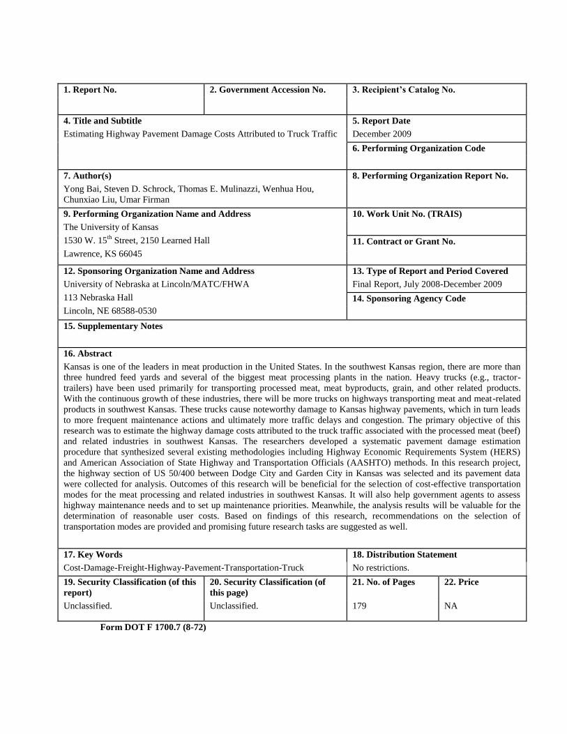
16. Abstract
Kansas is one of the leaders in meat production in the United States. In the southwest Kansas region, there are more than
three hundred feed yards and several of the biggest meat processing plants in the nation. Heavy trucks (e.g., tractor-
trailers) have been used primarily for transporting processed meat, meat byproducts, grain, and other related products.
With the continuous growth of these industries, there will be more trucks on highways transporting meat and meat-related
products in southwest Kansas. These trucks cause noteworthy damage to Kansas highway pavements, which in turn leads
to more frequent maintenance actions and ultimately more traffic delays and congestion. The primary objective of this
research was to estimate the highway damage costs attributed to the truck traffic associated with the processed meat (beef)
and related industries in southwest Kansas. The researchers developed a systematic pavement damage estimation
procedure that synthesized several existing methodologies including Highway Economic Requirements System (HERS)
and American Association of State Highway and Transportation Officials (AASHTO) methods. In this research project,
the highway section of US 50/400 between Dodge City and Garden City in Kansas was selected and its pavement data
were collected for analysis. Outcomes of this research will be beneficial for the selection of cost-effective transportation
modes for the meat processing and related industries in southwest Kansas. It will also help government agents to assess
highway maintenance needs and to set up maintenance priorities. Meanwhile, the analysis results will be valuable for the
determination of reasonable user costs. Based on findings of this research, recommendations on the selection of
transportation modes are provided and promising future research tasks are suggested as well.
17. Key Words 18. Distribution Statement
Cost-Damage-Freight-Highway-Pavement-Transportation-Truck No restrictions.
19. Security Classification (of this
report)
20. Security Classification (of
this page)
21. No. of Pages 22. Price
Unclassified. Unclassified. 179 NA
Form DOT F 1700.7 (8-72)
iii
Table of Contents
CHAPTER 1 INTRODUCTION ................................................................................... 1
1.1 Background .................................................................................................. 1
1.2 Research Objective and Scope .................................................................... 6
1.3 Research Methodology ................................................................................ 7
1.3.1 Literature Review.................................................................................. 7
1.3.2 Data collection ...................................................................................... 8
1.3.3 Data analyses ........................................................................................ 8
1.3.4 Conclusions and recommendations....................................................... 8
CHAPTER 2 LITERATURE REVIEW ........................................................................ 10
2.1 Fundamentals of Highway Maintenance ................................................. 10
2.1.1 Heavy-Vehicle Impact on Pavement Damage .................................... 11
2.1.2 Pavement Damage Cost Studies ......................................................... 17
2.2 Pavement Management System ................................................................ 24
2.2.1 Data Collection ................................................................................... 26
2.2.2 Pavement Deterioration Prediction ..................................................... 28
2.2.3 Cost Analysis ...................................................................................... 31
CHAPTER 3 HIGHWAY DAMAGE COSTS ATTRIBUTED TO TRUCK TRAFFIC .......... 32
FOR PROCESSED BEEF AND RELATED INDUSTRIES .............................................. 32
3.1 Cost Estimation Methodology ................................................................... 32
3.1.1 Background ......................................................................................... 32
3.2 Relevant Pavement Damage Models and Equations .............................. 33
3.2.1Traffic-Related Pavement Damage Functions ..................................... 33
3.2.2 Time-Related Deterioration of Pavements.......................................... 41
3.3 Pavement Damage Cost Analysis Procedure ........................................... 45
3.4 Data Input Requirements .......................................................................... 49
3.5.1 Calculation of ESAL Factors and Annual ESALs .............................. 51
3.5.2 Determination of the Pavement ESAL Lives...................................... 54
3.5.4 Damage Costs Attributed to Beef and Related Industries .................. 64
iv
CHAPTER 4 CASE STUDY IN SOUTHWEST KANSAS .............................................. 67
4.1 Processed Meat Industries in Southwest Kansas .................................... 67
4.1.1 Various Stages in the Movement of Cattle ......................................... 68
4.1.2 Cattle Feeding Industry ....................................................................... 69
4.1.3 Meat Processing Industry .................................................................... 71
CHAPTER 5 DATA COLLECTION FOR SOUTHWEST KANSAS CASE ........................ 73
5.1 Truckload data ........................................................................................... 73
5.2 Truck Characteristics and type ................................................................ 74
5.2.1 Truck Axle Configurations ................................................................. 75
5.3 Pavement Characteristics data ................................................................. 78
5.3.1 Pavement Type, Length and Structure ................................................ 79
5.3.2 Pavement Distress Survey and PSR Performance .............................. 85
5.3.3 Applying the Pavement Data in Pavement Deterioration Models ...... 85
CHAPTER 6 TRUCK VMT ASSOCIATED WITH THE PROCESSED BEEF AND RELATED
INDUSTRIES ............................................................................................... 88
6.1 Truck VMT for Transporting Feeder Cattle to Feed Yards ................. 93
6.1.1 Truck Travel Paths for Transporting Feeder Cattle to Feed Yards ..... 93
6.1.2 Truckloads for Transporting Feeder Cattle to Feed Yards ................. 97
6.2 Truck VMT for Transporting Grains to Feed Yards ........................... 100
6.3 Truck VMT for Transporting Finished Cattle to Meat Processing
Plants ................................................................................................... 101
6.3.1 Truck VMT for Transporting Cattle from Feed Yards in Southwest
Kansas to Meat Processing Plants ........................................................ 102
6.3.2 Truck VMT for Transporting Cattle from Outside of Southwest
Kansas to Meat Processing Plants ........................................................ 109
6.4 Truck VMT for Transporting Meat to U.S. Customers ....................... 113
6.5 Truck VMT for Transporting Meat Byproducts .................................. 115
6.6 Summary ................................................................................................... 117
CHAPTER 7 CONCLUSIONS AND RECOMMENDATIONS ....................................... 121
7.1 Conclusions ............................................................................................... 121
7.2 Recommendations .................................................................................... 124
v
REFERENCES ..................................................................................................... 126
APPENDIXES ...................................................................................................... 131
APPENDIX I ....................................................................................................... 132
APPENDIX II ...................................................................................................... 137
APPENDIX III ..................................................................................................... 146
APPENDIX IV ..................................................................................................... 155
APPENDIX V ...................................................................................................... 164
APPENDIX VI ..................................................................................................... 169
vi
List of Tables
Table 1.1 Total Daily & Annual Truck VMTs for Processed Meat and Related
Industries in Southwest Kansas (Bai et al. 2007) ......................................................... 6
Table 2.1 List of Research Projects on Pavement Damage ........................................ 12
Table 2.2 List of Research Projects on Maintenance Costs ........................................ 18
Table 3.1 Layer Coefficients Used to Compute Pavement Structural Numbers
(Tolliver 2000) ............................................................................................................ 43
Table 3.2 Suggested Layer Coefficients for Fractured Slab Pavements (AASHTO
1993) ........................................................................................................................... 45
Table 3.3 Calculation of ESAL Factors and Annual ESALs ………………………. 55
Table 3.4 Calculation of Pavement ESAL Lives ……………………………………57
Table 3.5 Maintenance Cost Data for Studied Pavement Segments ........................... 56
Table 3.6 Maintenance Costs in Year 2007 U.S. Dollars ........................................... 59
Table 3.7 Average Annual Maintenance Costs per Mile Attributed to Truck Traffic ....
..................................................................................................................................... 62
Table 3.8 Pavement Maintenance Costs Results ……………………………………64
Table 3.9 Pavement Length of Major Highways in Southwest Kansas Region ......... 65
Table 5.1 US-50/400 Pavement Basic Data in Finney County ................................... 83
Table 5.2 US-50/400 Pavement Basic Data in Gray County ...................................... 83
Table 5.3 US-50/400 Pavement Basic Data in Ford County ...................................... 83
Table 5.4 Present Serviceability Rating (PSR) ........................................................... 87
Table 6.1 Details of Studied Pavement Segments ...................................................... 88
Table 6.2 Sequence for Allocating Feeder Cattle in Each County ............................. 97
Table 6.3 Total Truckloads and Truck VMT for Transporting Feeder Cattle to Feed
Yards ......................................................................................................................... 100
Table 6.4 Daily & Annual Truck VMT for Transporting Finished Cattle from
Southwest Kansas County Centroids to Excel Corporation (Bai et al. 2007) .......... 104
Table 6.5 Daily & Annual Truck VMT for Transporting Finished Cattle from
Southwest Kansas County Centroids to National Beef in Dodge City (Bai et al. 2007)
................................................................................................................................... 105
vii
Table 6.6 Daily & Annual Truck VMT for Transporting Finished Cattle from
Southwest Kansas County Centroids to National Beef in Liberal (Bai et al. 2007) .......
................................................................................................................................... 106
Table 6.7 Daily & Annual Truck VMT for Transporting Finished Cattle from
Southwest Kansas County Centroids to Tyson Fresh Meats in Holcomb (Bai et al.
2007) ......................................................................................................................... 107
Table 6.8 Truckloads for Transporting Cattle from Counties to Meat Plants .......... 108
Table 6.9 Annual Truckloads for Transporting Finished Cattle from Outside of
Southwest Kansas to Four Meat processing Plants................................................... 111
Table 6.10 Truckloads for Transporting Cattle from Outside to Meat Plants .......... 111
Table 6.11 Total Truckloads and Truck VMT for Transporting Cattle to Meat Plants
................................................................................................................................... 112
Table 6.12 Total Annual Truck VMT on the Studied Pavement Segments in
Southwest Kansas (One-Way) .................................................................................. 119
Table 6.13 Total Daily & Annual Truck VMT on the Studied Highway Segments in
Southwest Kansas (Round-Trip) ............................................................................... 120
viii
List of Figures
Fig. 1.1 Feed Yards in Kansas (KDHE, 2005) ............................................................. 2 Fig. 1.2 Feed Yards in Southwest Kansas (KDHE, 2006)............................................ 3
Fig. 2.3 Effect of Treatment Timing on Repair Costs (AASHTO, 2001) .................. 25 Fig. 3.1 Theoretical Relationship Between Loss of Pavement Serviceability and Time
(Tolliver 2000) ............................................................................................................ 42 Fig. 3.2 Flowchart of Pavement Damage Cost Analysis Procedure ........................... 48 Fig. 3.3 PPI Change in Materials and Components for Construction from 1981 to
2007 (USDL 2007) ..................................................................................................... 58 Fig. 3.4 PPI Change in Construction Machinery and Equipment from 1981 to 2007
(USDL 2007) .............................................................................................................. 58
Fig. 3.5 Projected Future Annual Pavement Damage Costs Associated with Meat
Processed and Related Industries on the Studied Highway Section ........................... 66 Fig. 4.1 Sequence of the Kansas Meat Industry (Bai et al. 2007) .............................. 67
Fig. 5.1 Illustrative Truck Fleet Configuration ........................................................... 76 Fig. 5.2 Location Map of Highway Section Under Study .......................................... 79
Fig. 5.3 Typical Cross Section of a Conventional Flexible Pavement ....................... 80 Fig. 5.4 Typical Cross Section of a Full-Depth Asphalt Pavement ............................ 81 Fig. 5.5 Typical Cross Section of a Rigid Pavement .................................................. 81
Fig. 5.6 Pavement Types of the Studied Highway Segment ...................................... 82 Fig. 6.1 Southwest Kansas Highway Map (Source: KDOT 2005) ............................. 91
Fig. 6.2 Flowchart Showing the Procedure of the Estimation of Annual Truck VMT
Associated with Processed Beef and Related Industries............................................. 92
Fig. 6.4 Zone Analysis for Allocating Cattle in Southwest Kansas ........................... 95
1
Chapter 1 Introduction
1.1 Background
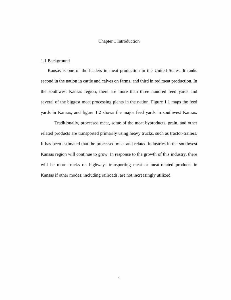
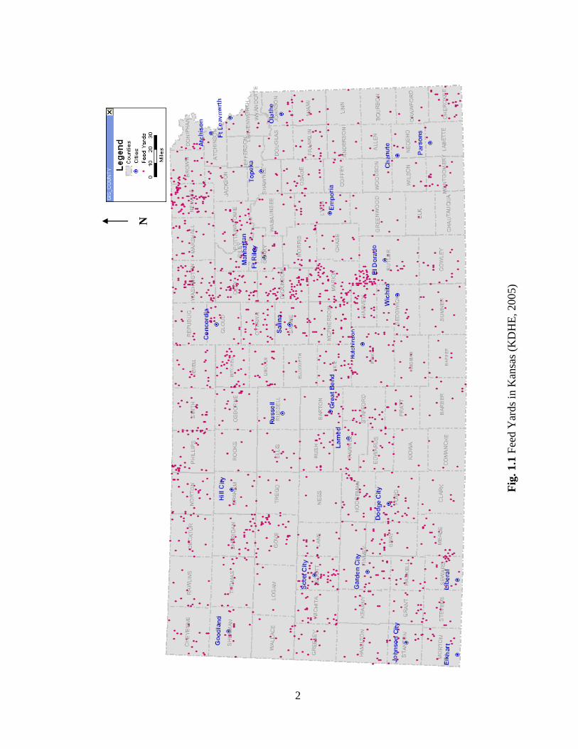
Kansas is one of the leaders in meat production in the United States. It ranks
second in the nation in cattle and calves on farms, and third in red meat production. In
the southwest Kansas region, there are more than three hundred feed yards and
several of the biggest meat processing plants in the nation. Figure 1.1 maps the feed
yards in Kansas, and figure 1.2 shows the major feed yards in southwest Kansas.
Traditionally, processed meat, some of the meat byproducts, grain, and other
related products are transported primarily using heavy trucks, such as tractor-trailers.
It has been estimated that the processed meat and related industries in the southwest
Kansas region will continue to grow. In response to the growth of this industry, there
will be more trucks on highways transporting meat or meat-related products in
Kansas if other modes, including railroads, are not increasingly utilized.
2
Fig
. 1.1
Fee
d Y
ards
in K
ansa
s (K
DH
E, 2005)
N
3
Fig
. 1.2
Fee
d Y
ards
in S
outh
wes
t K
ansa
s (K
DH
E, 2006)
N
4
With the growth in truck traffic, highways will be overburdened. Increased
traffic will increase traffic congestion, highway maintenance costs, frequency of
roadway replacement, air pollution, fuel consumption, and travel times for road users.
To address this concern, a research project was conducted in 2006 to study the
utilization status of available transportation modes—including truck, railroad, and
intermodal—in the processed meat and related industries in southwest Kansas region
and their impacts on local and regional economies (Bai et al. 2007). This study
concentrated on the processed beef and related industries, and included the counties
of Clark, Comanche, Edwards, Finney, Ford, Grant, Gray, Greeley, Hamilton,
Haskell, Hodgeman, Kearny, Kiowa, Lane, Meade, Morton, Ness, Pawnee, Rush,
Scott, Seward, Stanton, Stevens, and Wichita.
To achieve the research goal, Bai et al. reviewed the current state-of-practice
for the transportation of processed meat, meat by-products, feed grain, and industry-
related products. This was followed by an evaluation of the pros and cons of different
transportation modes used to support the meat and related industries. Second, the
TransCAD software program was used to facilitate GIS-based analyses including
mapping the feed yards and processed meat plants in Kansas and in southwest Kansas
region. Third, researchers collected related transportation data from various sources
including state and federal government agencies, trucking and railroad companies,
processed meat plants, feed yard owners, trade organizations, local economic
development offices, and Web sites. To gather first-hand information, two site visits
to southwest Kansas, two local visits to trade organizations, and telephone interviews
5
were conducted by the research team. Finally, based on the collected data, the vehicle
miles of travel (VMT) generated by the processed meat and related industries in
southwest Kansas were estimated. The total VMTs were divided into six categories of
transit as indicated in the following list (Bai et al. 2007):
Feeder cattle to feed yards in southwest Kansas;
Feed grain to feed yards in southwest Kansas;
Finished cattle to meat processing plants in southwest Kansas;
Boxed beef to customers in the United States;
Meat byproducts to overseas customers; and
Boxed beef to overseas customers (currently market closed)
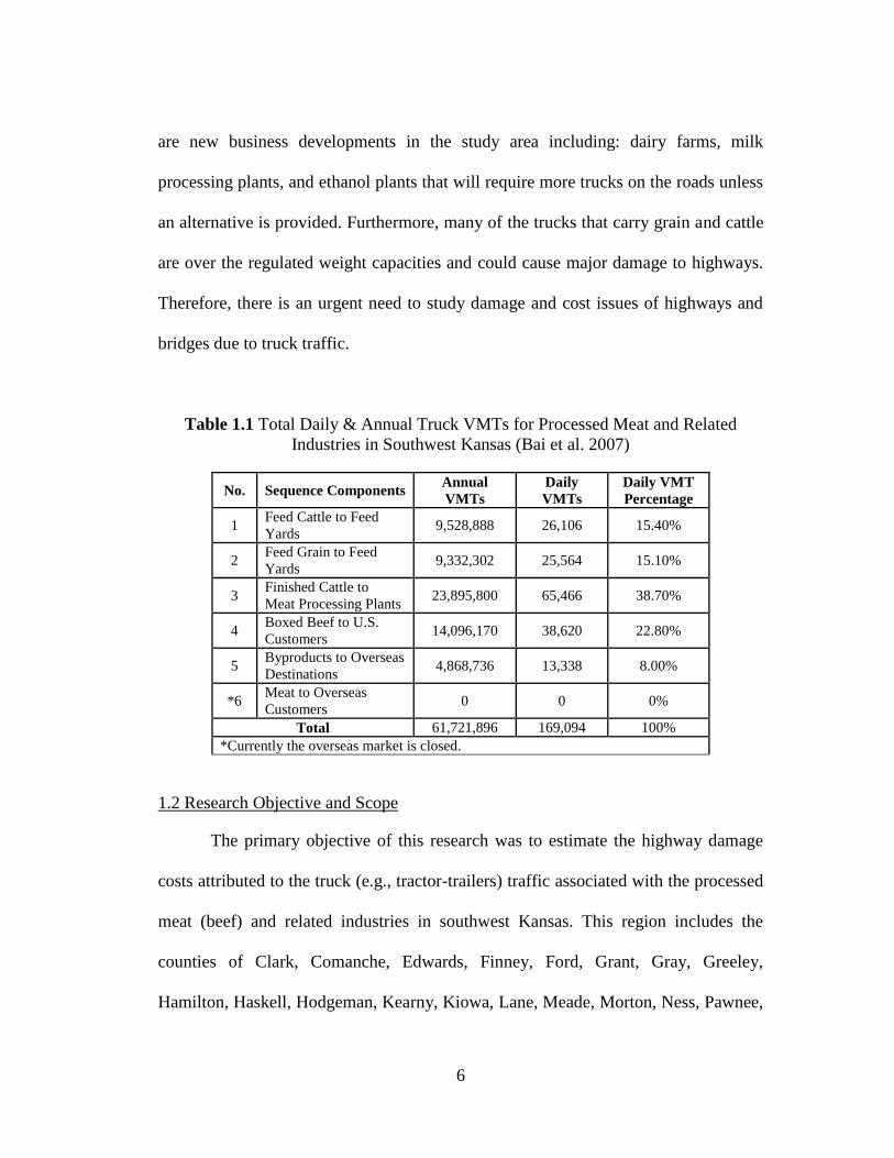
Table 1.1 presents the final results of the total daily and annual truck VMT of
roundtrip shipments generated due to business activities associated with the processed
meat and related industries in southwest Kansas. The research team concluded that
there was a need to diversify the utilization of different modes available under the
current freight transportation structure. They recommended promising improvements
to relieve the traffic burden caused by the processed meat and related industries in
Kansas (Bai et al. 2007).
A high truck VMT can cause noteworthy damage to highways and bridges,
resulting in more frequent maintenance work. There is high truck traffic on highways
50/400 and 54 in southwest Kansas that could cause rapid deterioration of these
highways and higher accident rates. Also, if the planned new meat plant in Hooker,
Oklahoma is built, it will increase the truck traffic on these roads. In addition, there
6
are new business developments in the study area including: dairy farms, milk
processing plants, and ethanol plants that will require more trucks on the roads unless
an alternative is provided. Furthermore, many of the trucks that carry grain and cattle
are over the regulated weight capacities and could cause major damage to highways.
Therefore, there is an urgent need to study damage and cost issues of highways and
bridges due to truck traffic.
Table 1.1 Total Daily & Annual Truck VMTs for Processed Meat and Related
Industries in Southwest Kansas (Bai et al. 2007)
No. Sequence Components Annual
VMTs
Daily
VMTs
Daily VMT
Percentage
1 Feed Cattle to Feed
Yards 9,528,888 26,106 15.40%
2 Feed Grain to Feed
Yards 9,332,302 25,564 15.10%
3 Finished Cattle to
Meat Processing Plants 23,895,800 65,466 38.70%
4 Boxed Beef to U.S.
Customers 14,096,170 38,620 22.80%
5 Byproducts to Overseas
Destinations 4,868,736 13,338 8.00%
*6 Meat to Overseas
Customers 0 0 0%
Total 61,721,896 169,094 100%
*Currently the overseas market is closed.
1.2 Research Objective and Scope
The primary objective of this research was to estimate the highway damage
costs attributed to the truck (e.g., tractor-trailers) traffic associated with the processed
meat (beef) and related industries in southwest Kansas. This region includes the
counties of Clark, Comanche, Edwards, Finney, Ford, Grant, Gray, Greeley,
Hamilton, Haskell, Hodgeman, Kearny, Kiowa, Lane, Meade, Morton, Ness, Pawnee,
7
Rush, Scott, Seward, Stanton, Stevens, and Wichita. Results of the study will be used
to select cost-effective transportation modes for the meat processing and related
industries in southwest Kansas region, to better assess highway maintenance needs,
and to establish maintenance priorities. The analysis results could be utilized to
determine reasonable user costs.
It has been estimated that several highway sections, including US 50/400 from
Dodge City to Garden City, carried a significant proportion of the truck traffic
generated by the processed beef and related industries in southeast Kansas (Bai et al.
2007). A significant percentage of the consequent maintenance costs for these
highway sections were attributed to the heavy truck traffic. In this research project,
the highway section of US 50/400 from Dodge City to Garden City was selected and
its pavement data were collected for analysis.
1.3 Research Methodology
The research objective was achieved with four-steps: a literature review, data
collection, data analyses, and conclusions and recommendations.
1.3.1 Literature Review
A comprehensive literature review was conducted first to gather the state-of-
practice for the transportation of processed meat, meat by-products, feed grain, and
industry-related products as well as to understand the highway damage associated
with large heavy vehicles. The review also included the literature on Pavement
Management Systems (PMS), which was a key element in the pavement data

8
collection step. Additionally, this analysis synthesized knowledge from sources such
as journals, conference proceedings, periodicals, theses, dissertations, special reports,
and government documents.
1.3.2 Data collection
To estimate highway damage costs associated with the processed beef and
related industries, several types of data were required. To this end, truckload data on
the study highway section, truck characteristics, pavement characteristics, and
pavement maintenance cost data were collected from various sources.
1.3.3 Data analyses
In this study, the researcher used a systematic pavement damage estimation
procedure that synthesized several existing methodologies. These include functions
developed by Highway Economic Requirements System (HERS) and American
Association of State Highway and Transportation Officials (AASHTO). The
researcher analyzed the collected data and utilized it in the estimation procedure to
determine annual highway damage costs attributed to processed beef related
industries in southwest Kansas.
1.3.4 Conclusions and recommendations
Based on the results of the data analyses, the researcher drew conclusions and
made recommendations accordingly. The conclusions included important analysis
findings, possible analysis variations, and research contributions. In addition,

9
recommendations on utilization of transportation modes, transportation infrastructure,
and promising future research were provided.
10
Chapter 2 Literature Review
A comprehensive literature review was conducted to structure the research background.
The knowledge from this review was synthesized and will be presented in this chapter. First, the
authors will supply a brief introduction to the processed meat and related industries in southwest
Kansas. This will include the individual stages of the meat processing industry and the product
transportation process. Then, the fundamental knowledge of highway maintenance will be
provided to highlight the highway damage caused by heavy-vehicle traffic. Previous studies on
heavy-vehicle-related highway cost estimation will also be examined in this section. Finally, the
authors will describe the pavement management system and its key components such as
pavement data collection, pavement deterioration prediction, and maintenance cost analysis. The
literature review includes journals, conference proceedings, periodicals, theses, dissertations,
special reports, and government documents.
2.1 Fundamentals of Highway Maintenance
―Highway maintenance‖ is defined as the function of preserving, repairing, and restoring
a highway and keeping it in condition for safe, convenient, and economical use. ―Maintenance‖
includes both physical maintenance activities and traffic service activities. The former includes
activities such as patching, filling joints, and mowing. The latter includes painting pavement
markings, erecting snow fences, removing snow, ice, and litter. Highway maintenance programs
are designed to offset the effects of weather, vandalism, vegetation growth, and traffic wear and
damage, as well as deterioration due to the effects of aging, material failures, and construction
faults (Wright and Dixon 2004).
11
2.1.1 Heavy-Vehicle Impact on Pavement Damage
Commonly identified pavement distress associated with heavy vehicles can be
characterized as fatigue cracking and rutting. On rigid pavements damage includes transverse
cracking, corner breaking, and cracking on the wheel paths. Flexible pavements and granular
roads are most susceptible to rutting. In all cases, cracking and rutting increase pavement
roughness and reduce pavement life.
Trucking has become the most popular mode of freight transportation because of its
efficiency and convenience, and this preference has resulted in increased highway maintenance
costs nationwide. To date, a large amount of research effort has been devoted to the study of the
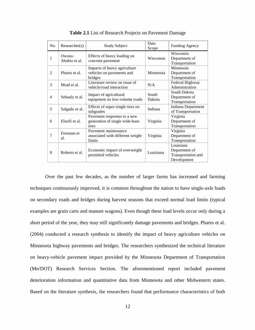
pavement damage associated with heavy vehicles. Eight studies are summarized in this section as
shown in Table 2.1.
In 2001, the Wisconsin Department of Transportation-District Seven released a Report of
Early Distress for a 6.5-mile stretch of US 8 and an 8-mile stretch of US 51 near Rhinelander,
WI (Owusu-Ababio et al. 2005). An investigation of the causes for premature failures concluded
that overloaded logging trucks were a key factor leading to the early failure of doweled jointed
plain concrete pavements (JPCP). Based on the recommendations from this report, Owusu-
Ababio et al. (2005) developed design guidelines for heavy truck loading on concrete pavements
in Wisconsin.
12
Table 2.1 List of Research Projects on Pavement Damage
No. Researcher(s) Study Subject Data
Scope Funding Agency
1 Owusu-
Ababio et al.
Effects of heavy loading on
concrete pavement Wisconsin
Wisconsin
Department of
Transportation
2 Phares et al.
Impacts of heavy agriculture
vehicles on pavements and
bridges
Minnesota
Minnesota
Department of
Transportation
3 Mrad et al. Literature review on issue of
vehicle/road interaction N/A
Federal Highway
Administration
4 Sebaaly et al. Impact of agricultural
equipment on low-volume roads
South
Dakota
South Dakota
Department of
Transportation
5 Salgado et al. Effects of super-single tires on
subgrades Indiana
Indiana Department
of Transportation
6 Elseifi et al.
Pavement responses to a new
generation of single wide-base
tires
Virginia
Virginia
Department of
Transportation
7 Freeman et
al.
Pavement maintenance
associated with different weight
limits
Virginia
Virginia
Department of
Transportation
8 Roberts et al. Economic impact of overweight
permitted vehicles Louisiana
Louisiana
Department of
Transportation and
Development
Over the past few decades, as the number of larger farms has increased and farming
techniques continuously improved, it is common throughout the nation to have single-axle loads
on secondary roads and bridges during harvest seasons that exceed normal load limits (typical
examples are grain carts and manure wagons). Even though these load levels occur only during a
short period of the year, they may still significantly damage pavements and bridges. Phares et al.
(2004) conducted a research synthesis to identify the impact of heavy agriculture vehicles on
Minnesota highway pavements and bridges. The researchers synthesized the technical literature
on heavy-vehicle pavement impact provided by the Minnesota Department of Transportation
(Mn/DOT) Research Services Section. The aforementioned report included pavement
deterioration information and quantitative data from Minnesota and other Midwestern states.
Based on the literature synthesis, the researchers found that performance characteristics of both
13
rigid and flexible pavements were adversely affected by overweight implements. The wide wheel
spacing and slow movement of heavy agricultural vehicles further exacerbated the damage on
roadway systems. The researchers also found that two structural performance measures—
bending and punching—were used in the literature for evaluating the impact of agricultural
vehicles on bridges. A comparison between the quantified structural metrics of a variety of
agricultural vehicles and those of the bridge design vehicle yielded two important conclusions.
(1) The majority of the agricultural vehicles investigated created more extreme structural
performance conditions on bridges as it pertains to bending behavior. (2) Several of the
agricultural vehicles exceeded design vehicle structural performance conditions based on
punching.
Many studies have been done to reveal the relationship between trucks and pavement
damage. Mrad et al. (1998) conducted a literature review on these studies as a part of the Federal
Highway Administration‘s (FHWA) Truck Pavement Interaction research program on truck size
and weight. This review focused on spatial repeatability of dynamic wheel loads produced by
heavy vehicles and its effect on pavement damage. The review included several studies
identifying the effects of the environment, vehicle design, vehicle characteristics and operating
conditions on pavement damage. According to the review, suspension type and characteristics, as
well as tire type and configuration, were major contributors to pavement deterioration. The
literature review also remarked on the relationship among spatial repeatability of dynamic wheel
forces, suspension type, and road damage.
Different types of vehicles cause different types of damage to pavements. Vehicle
loading on highway pavement is corresponds closely to axle weight and configuration. Sebaaly
et al. (2002) evaluated the impact of agricultural equipment on the response of low-volume roads
14
in the field. In this evaluation process, a gravel pavement section and a blotter pavement section
in South Dakota were tested with agricultural equipment. Each section had pressure cells in the
base and subgrade, and deflection gauges to measure surface displacement. Field tests were
carried out in different conditions in 2001. Test vehicles included two terragators (a specialized
tractor used to fertilize crops), a grain cart, and a tracked tractor. The field testing program
collected the pavement responses under five replicates of each combination of test vehicle and
load level. This data was compared with those responses under the 18,000-lb single-axle truck--a
figure which represented the 18,000-lb equivalent single axle load (ESAL) in the AASHTO
design guide. Data were examined for repeatability, and then the average of the most repeatable
set of measurements were calculated and analyzed. Results indicated that agricultural equipment
could be significantly more damaging to low-volume roads than an 18,000-lb single-axle truck.
They found that the impacts depended on factors such as season, load level, thickness of crushed
aggregate base of roads, and soil type. The researchers recommended that a highway agency
could effectively reduce this impact by increasing the thickness of the base layer and keeping the
load as close to the legal limit as possible.
In recent years, super-single tires have gradually replaced conventional dual tires due to
their efficiency and economic features. However, earlier studies on previous generations of
single wide-base tires have found that the use of super-single tires would result in a significant
increase in pavement damage compared to dual tires. Salgado et al. (2002) investigated the
effects of super-single tires on subgrades for typical road cross-sections using plane-strain (2D),
and 3D static and dynamic finite-element (FE) analyses. The analyses focused on sand and clay
subgrades rather than on asphalt and base layers. The subgrades were modeled as saturated in
order to investigate the effects of pore water pressures under the most severe conditions. By
15
comparing the difference of strains in the subgrade induced by super-single tires with those
induced by dual tires for the same load, the effects of overlay and subgrade improvements were
apparent. Several FE analyses were conducted by applying super-heavy loads to the typical
Indiana pavements using elastic-plastic analyses in order to assess the performance of the typical
pavements under the super heavy loads. The analyses showed that super-single tires caused more
damage to the subgrade and that the current flexible pavement design methods were inferior
considering the increased loads by super-single tires. In addition, the researchers proposed
several recommendations to improve the pavement design method that would decrease the
adverse effects of super-single tires on the subgrades.
Elseifi et al. (2005) measured pavement responses to a new generation of single wide-
base tire compared with dual tires. The new generation of single wide-base tires has a wider
tread and a greater load-carrying capacity than conventional wide-base tires; therefore this design
has been strongly supported by the trucking industry. The primary objective of their study was to
quantify pavement damage caused by conventional dual tires and two new generations of wide-
base tires (445/50R22.5 and 455/55R22.5) by using FE analysis. Fatigue cracking, primary
rutting, secondary rutting, and top-down cracking were four main failure mechanisms considered
in the pavement performance analysis. In the FE models developed for this research, geometry
and dimensions were selected to simulate the axle configurations typically used in North
America. The models also considered actual tire tread sizes and applicable contact pressure for
each tread, and incorporated laboratory-measured pavement material properties. The researchers
calibrated and validated the models based on stress and strain measurements obtained from the
experimental program. Pavement damage was calculated at a reference temperature of 77 °F and
16
at two vehicle speeds--5 and 65 mph. Results indicated that the new generations of wide-base
tires would cause the same or greater pavement damage than conventional dual tires.
Because heavy trucks cause more damage to highways, it is of interest to federal and state
legislatures whether the current permitted weight limit reflects the best tradeoff between trucking
productivity and highway maintenance cost. A study (Freeman et al. 2002) was mandated by
Virginia‘s General Assembly to determine if pavements in the southwest region of the state
under higher allowable weight limit provisions had greater maintenance and rehabilitation
requirements than pavements bound by lower weight limits elsewhere. This study included
traffic classification, weight surveys, an investigation of subsurface conditions, and
comprehensive structural evaluations, which were conducted at 18 in-service pavement sites.
Visible surface distress, ride quality, wheel path rutting, and structural capacity were measured
during 1999 and 2000. A subsurface investigation was conducted at each site in October 1999 to
document pavement construction history and subgrade support conditions. In addition, a survey
consisting of vehicle counts, classifications, and approximate measurements of weights was
administered to collect site-specific information about traffic volume and composition. The
results were used to estimate the cost of damage attributed only to the net increase in allowable
weight limits. The study concluded that pavement damage increased drastically with relatively
small increases in truck weight. The cost of damage to roadway pavements in those counties with
a higher allowable weight limit was estimated to be $28 million over a 12-year period. Among
other factors, this figure did not include costs associated with damage to bridges and motorist
delays through work zones.
In Louisiana, Roberts (2005) completed a study to assess the economic impact of
overweight vehicles hauling timber, lignite coal, and coke fuel on highways and bridges. First,
17
researchers identified 1,400 key control sections on Louisiana highways that carried timber, 4
control sections that carried lignite coal, and approximately 2,800 bridges that were involved in
the transport of both of these commodities. Second, a calculation methodology was developed to
estimate the overlays required to support the transportation of these commodities under the
various gross vehicle weight (GVW) scenarios. Three different GVW scenarios were selected for
this study including: (1) 80,000 lbs., (2) 86,600 lbs. or 88,000 lbs., and (3) 100,000 lbs. Finally, a
methodology for analyzing the effect of these loads on pavements was developed and it involved
determining the overlay thickness required to carry traffic from each GVW scenario for the
overlay design period. In addition, a method of analyzing the bridge costs was developed using
the following two steps: (1) determining the shear, moment and deflection induced on each
bridge type and span, and (2) developing a cost of repairing fatigue damage for each vehicle
passage with a maximum tandem load of 48,000 lbs. This analysis showed that 48 kilo pound
(kip) axles produced more pavement damage than the current permitted GVW for timber trucks
and caused significant bridge damage at all GVW scenarios included in the study. The
researchers recommended that the legislature eliminate the 48-kip maximum individual axle load
and keep GVWs at the current level, but increase the permit fees to sufficiently cover the
additional pavement costs produced by overweight vehicles.
2.1.2 Pavement Damage Cost Studies
A total of about 4,000,000 miles of roads, including 46,572 miles of Interstate highways
and over 100,000 miles of other national highways, form the backbone of the United States
highway infrastructure. Careful planning considerations and wise investment decisions are
necessary for the maintenance of the nation‘s massive infrastructure to support a sufficient level
of operations and provide a satisfying degree of serviceability. Studies have found that trucks
18
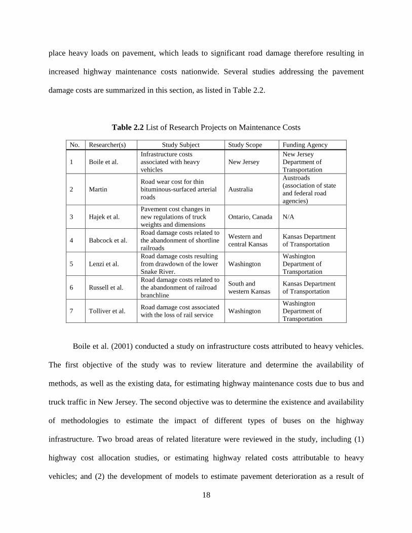
place heavy loads on pavement, which leads to significant road damage therefore resulting in
increased highway maintenance costs nationwide. Several studies addressing the pavement
damage costs are summarized in this section, as listed in Table 2.2.
Table 2.2 List of Research Projects on Maintenance Costs
No. Researcher(s) Study Subject Study Scope Funding Agency
1 Boile et al.
Infrastructure costs
associated with heavy
vehicles
New Jersey
New Jersey
Department of
Transportation
2 Martin
Road wear cost for thin
bituminous-surfaced arterial
roads
Australia
Austroads
(association of state
and federal road
agencies)
3 Hajek et al.
Pavement cost changes in
new regulations of truck
weights and dimensions
Ontario, Canada N/A
4 Babcock et al.
Road damage costs related to
the abandonment of shortline
railroads
Western and
central Kansas
Kansas Department
of Transportation
5 Lenzi et al.
Road damage costs resulting
from drawdown of the lower
Snake River.
Washington
Washington
Department of
Transportation
6 Russell et al.
Road damage costs related to
the abandonment of railroad
branchline
South and
western Kansas
Kansas Department
of Transportation
7 Tolliver et al. Road damage cost associated
with the loss of rail service Washington
Washington
Department of
Transportation
Boile et al. (2001) conducted a study on infrastructure costs attributed to heavy vehicles.
The first objective of the study was to review literature and determine the availability of
methods, as well as the existing data, for estimating highway maintenance costs due to bus and
truck traffic in New Jersey. The second objective was to determine the existence and availability
of methodologies to estimate the impact of different types of buses on the highway
infrastructure. Two broad areas of related literature were reviewed in the study, including (1)
highway cost allocation studies, or estimating highway related costs attributable to heavy
vehicles; and (2) the development of models to estimate pavement deterioration as a result of
19
vehicle-pavement interactions. The existing highway cost allocation methods were categorized
into four groups: cost-occasioned approaches, benefit-based approaches, marginal cost
approaches, and incremental approaches. Federal, as well as several state highway cost
allocation, studies were reviewed in the research and all used cost-occasioned approaches. The
approaches used in these studies varied in data requirements, ease of use and updating, as well as
output detail. Regarding pavement deterioration estimation, several types of models had been
developed for flexible and rigid pavements, including statistical models, subjective models,
empirical deterioration models, mechanistic/empirical models, and mechanized models. In
addition, the researchers reviewed literature addressing bus impacts on pavements. Finally, the
researchers reached two conclusions. (1) Performing a cost allocation study would be highly
recommended since it could help develop a clear picture of the cost responsibility of each vehicle
class. It would determine whether changes need to be made in order to charge each vehicle class
its fair share of cost responsibility. (2) Additionally, two of the statewide cost allocation
approaches might provide useful guidelines in developing a relatively easy to use and updated
model. This research also presented a proposed method for estimating bus impacts on New
Jersey highways, which was based on estimates of ESALs with a step-by-step guide on how to
apply the method.
Load-related road wear is considered to be an approximation for the marginal cost of road
damage. Due to high axle loads, heavy vehicles are considered to be primarily responsible for
road wear. Martin (2002) estimated road wear cost for thin bituminous-surfaced arterial roads in
Australia, which was based on the following two approaches: (1) a statistical relationship
between the road maintenance costs and a heavy-vehicle-road-use variable; and (2) a pavement
deterioration model that estimated the portion of load-related road wear based on pavement
20
deterioration predictions for thin bituminous-surfaced granular pavements. The data used in the
study were collected from the following sources which cover all Australian states. (1) 255
arterial road samples, composed of 171 rural and 84 urban samples, varying in average length
from 30 km (18.6 miles) in rural area to 0.15 km (0.09 miles) in urban areas; (2) three years of
maintenance expenditure data in estimating the annual average maintenance cost at each road
sample; and 3) estimates of road use at each road sample. The study found that 55% to 65% of
the recent estimates of road wear cost were due to heavy vehicles for the average level of traffic
loading on the bituminous surfaced arterial road network of Australia. The researchers suggested
that the fourth power of the law-based ESAL road-use variable could be used for estimating road
wear costs.
Hajek et al. (1998) developed a marginal cost method for estimating pavement cost from
proposed changes in regulations governing truck weights and dimensions in Ontario, Canada.
The procedure was part of a comprehensive study undertaken by the Ontario Ministry of
Transportation in response to government and industry initiatives to harmonize Ontario‘s truck
regulations with those in surrounding jurisdictions. The study investigated the individual impacts
of four proposed alternative regulatory scenarios. The differences between the scenarios were
relatively small and were directed only at trucks with six or more axles. The procedure for
assessing pavement costs consisted of three phases: (1) identification of new traffic streams; (2)
allocation of these new traffic streams to the highway system; and (3) assessment of cost impacts
of the new traffic streams on the pavement network. The marginal pavement cost of truck
damage was defined as a unit cost of providing pavement structure for one additional passage of
a unit truckload (expressed as ESAL). The marginal pavement costs were calculated as
annualized life-cycle costs and expressed as equivalent uniform annual costs (EUACs). The
21
study concluded that: (1) the marginal cost method could be used to quantify relatively minor
changes in axle weights and pavement damage caused by any axle load, or axle load arrangement
for both new and in-service pavements; and (2) the highway type (or truck volumes associated
with the highway type) had a major influence on marginal cost.
Babcock et al. (2003) conducted a study to estimate road damage costs caused by
increased truck traffic resulting from the proposed abandonment of shortline railroads serving
western and central Kansas. The study area included the western two-thirds of the state. The four
shortlines assumed to be abandoned were: the Central Kansas Railroad (CKR), the Kyle
Railroad, the Cimarron Valley Railroad (CVR), and the Nebraska, Kansas and Colorado Railnet
(NKC). Their objective was achieved in a three-step approach. First, a transportation cost model
was developed to compute how many wheat car loadings occurred at each station on each of the
four-shortline railroads in the study area. Then, the shortline railroad car loadings at each station
were converted to truckloads at a ratio of one rail carload equal to four truck loads. Finally, a
pavement damage model by Tolliver (2000) was employed to calculate the additional damage
costs for county and state roads attributed to the increased grain trucking due to shortline
abandonment. The study also used a time decay model and an ESAL model to examine how
increased truck traffic affected pavement service life. Pavement data inputs required by the
models used in the study included designation as US, Kansas, or Interstate highway;
transportation route number; beginning and ending points of highway segments by street, mile
marker, or other landmarks; length of pavement segment; soil support values; pavement
structural numbers; annual 18-kip traffic loads; and remaining 18-kip traffic loads until
substantial maintenance or reconstruction. These data were obtained from the KDOT CANSYS
database. The road damage cost resulting from abandonment of the short line railroads in the
22
study area could be divided into two parts: (1) costs associated with truck transportation of wheat
from farms to county elevators; and (2) costs of truck transportation of wheat from county
elevators to shuttle train stations and terminal elevators. The study found that the shortline
railroad system in the study area annually saved $57.8 million in road damage costs.
In eastern Washington, grain shippers were utilizing the Lower Snake River for
inexpensive grain transportation. However, with longer distances, the truck-barge grain
transportation resulted in higher damage costs for the principal highways in this geographical
area. Lenzi et al. (1996) conducted a study to estimate the deduction of the state and county road
damage costs in Washington by proposing a drawdown usage of the Lower Snake River. The
researchers proposed two potential drawdown scenarios. Scenario I assumed that the duration of
drawdown was from April 15 to June 15; and scenario II assumed that the duration of the
drawdown was from April 15 to August 15. During the drawdown, trucking would be the only
assumed shipping mode to the nearest elevators with rail service. Since the average length of
haul for a truck to an elevator was estimated at 15 miles, as compared with 45 miles for truck-
barge movements, the shifting from truck-barge mode to truck-rail mode would result in less
truck miles traveled and thus would cause a significant reduction of highway damage. Based on a
series of assumptions suggested by similar studies, the total road damage costs before the Lower
Snake River drawdown was estimated as $1,257,080 for Scenario I. The road damage cost after
Scenario I drawdown was calculated in a similar manner at $459,770, or 63% less than the pre-
drawdown cost. For scenario II, the drawdown was estimated to be able to reduce road damage
costs by $1,225,540, or 63%, as opposed to the pre-drawdown costs which were estimated as
$3,352,240. The researchers concluded that with adequate rail car supply, both drawdown
23
scenarios would decrease the system-wide highway damage costs, although certain roadways
might experience accelerated damages.
Russell et al. (1996) conducted a study to estimate potential road damage costs resulting
from a hypothetical abandonment of 800 miles of railroad branchline in south central and
western Kansas. First, the researchers adopted a wheat logistics network model developed by
Chow (1985) to measure truck and rail shipment changes in grain transportation due to railroad
abandonment. The model contained 400 simulated farms in the study area. The objective
function of this model was to minimize the total transport cost of moving Kansas wheat from the
simulated farms to county elevators, from county elevators to Kansas railroad terminals, and then
from railroad terminals to export terminals in Houston, Texas. The model was employed for both
the base case (truck and railroad wheat movements, assuming no abandonment of branchlines)
and the study case (after the abandonment of branch lines). Second, the researchers measured the
pavement life of each highway segment in ESALs using Highway Performance Monitoring
System (HPMS) pavement functions. Finally, they estimated road damage in ESALs for each
type of truck by using the AASHTO traffic equivalency functions. Results indicated that annual
farm-to-elevator road damage costs before abandonment totaled $638,613 and these costs would
increase by $273,359 after abandonment. Elevator-to-terminal road damage costs before the
abandonment were $1,451,494 and would increase by $731,231 after the abandonment. Thus the
total abandonment related road damage costs would add up to $1,004,590.
Tolliver et al. (1994) developed a method to measure road damage cost associated with
the decline or loss of rail service in Washington State. Three potential scenarios were assumed in
the study: (1) the system-wide loss of mainline rail services in Washington; (2) the loss of all
branchline rail service in Washington; and (3) the diversion of all growth in port traffic to trucks
24
due to the potential loss of railroad mainline capacity. The study used AASHTO procedures to
estimate pavement deterioration rates and HPMS damage functions to measure the pavement life
of highway segments in ESALs. The research objective was achieved by using the following
steps: (1) defining the maximum feasible life of an impacted pavement in years, (2) determining
the life of a pavement in terms of traffic by using a standard measurement of ESALs, (3)
computing the loss of Present Serviceability Rating (PSR) from a time decay function for a
typical design performance period, (4) calculating an average cost per ESAL, and (5) computing
the avoidable road damage cost if the railroads were not abandoned. For Scenario 1, the
researchers estimated that the incremental annual pavement resurfacing cost would be $65
million and the annual pavement reconstruction cost would be $219.6 million. For Scenario 2,
the study found that, with different truck configurations, the annual resurfacing costs would
range from $17.4 to $28.5 million and the annual reconstruction cost would vary from $63.3
million to $104 million. In Scenario 3, the incremental annual pavement resurfacing costs would
be $63.3 million and the annual reconstruction cost would be $227.5 million.
2.2 Pavement Management System
In the past, pavements were maintained but not managed. Life-cycle costing and priority
were not considered as important factors in the selection of maintenance and rehabilitation
(M&R) techniques. Today‘s economic environment requires a more systematic approach to
determining M&R needs and priorities (Shahin 1994). All pavements deteriorate over time due
to traffic and environment. The growth of truck traffic is of special importance to pavement
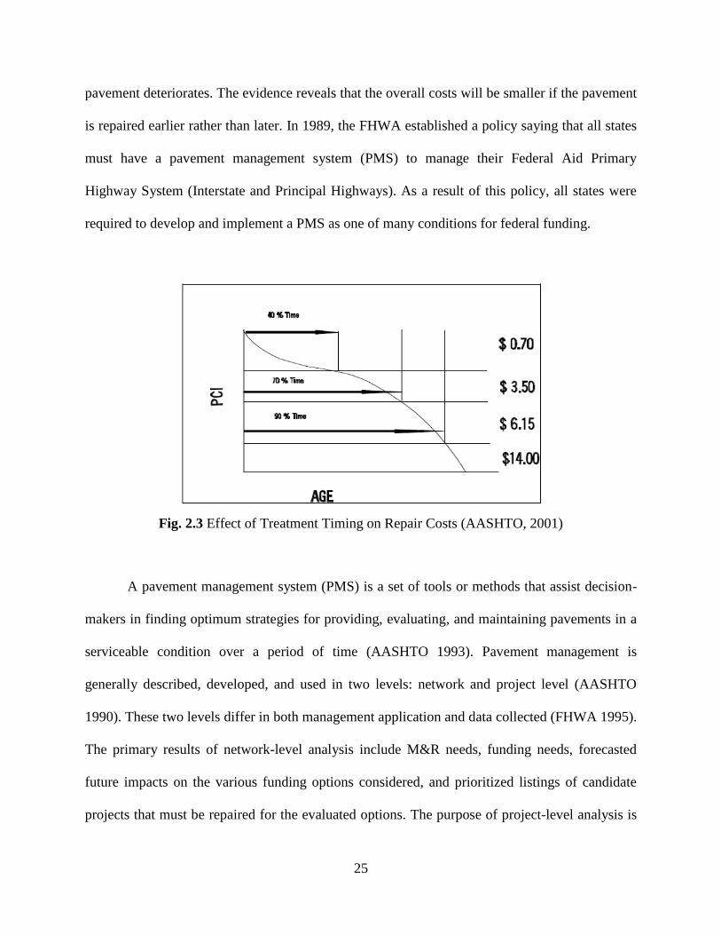
engineers and managers since it is one major cause of pavement deterioration. Figure 2.3 is a
curve that has been normally used to demonstrate the relationship between repair time and cost.
It shows the average rate of deterioration for an agency and the change in repair costs as the
25
pavement deteriorates. The evidence reveals that the overall costs will be smaller if the pavement
is repaired earlier rather than later. In 1989, the FHWA established a policy saying that all states
must have a pavement management system (PMS) to manage their Federal Aid Primary
Highway System (Interstate and Principal Highways). As a result of this policy, all states were
required to develop and implement a PMS as one of many conditions for federal funding.
Fig. 2.3 Effect of Treatment Timing on Repair Costs (AASHTO, 2001)
A pavement management system (PMS) is a set of tools or methods that assist decision-
makers in finding optimum strategies for providing, evaluating, and maintaining pavements in a
serviceable condition over a period of time (AASHTO 1993). Pavement management is
generally described, developed, and used in two levels: network and project level (AASHTO
1990). These two levels differ in both management application and data collected (FHWA 1995).
The primary results of network-level analysis include M&R needs, funding needs, forecasted
future impacts on the various funding options considered, and prioritized listings of candidate
projects that must be repaired for the evaluated options. The purpose of project-level analysis is
26
to provide the most cost-effective, feasible, and original design as a possible strategy for the
maintenance, rehabilitation, or reconstruction for a selected section of pavement within available
funds and other constraints (AASHTO 2001). Generally speaking, a PMS contains three primary
components (USDOT and FHWA 1998): (1) data collection: including inventory, history,
condition survey, traffic, and database; (2) analyses: including condition, performance,
investment, engineering and feedback analyses; and (3) update.
In the past three decades, PMSs have significantly improved. The early systems used
simple data-processing methods to evaluate and rank candidate pavement rehabilitation projects
only based on current pavement condition and traffic. Future pavement condition forecasting and
economic analyses were not considered in such systems. Systems developed in the 1990s use
integrated techniques of performance prediction, network- and project-level optimization, multi-
component prioritization, and geographic information systems (GIS) (Kulkarni and Miller 2003).
A mature PMS includes three key components: data collection, deterioration prediction, and cost
analysis, all of which are described in the following sections.
2.2.1 Data Collection
Data collection is an essential element of an efficient PMS. The data collection program
should focus on the following objectives: timeliness of collecting, processing, and recording data
in the system; accuracy and precision of the data collected; and integration. The major data
components include the following:
Inventory: physical pavement features including the number of lanes, length, width,
surface type, functional classification, and shoulder information;
History: project dates, types of construction, reconstruction, rehabilitation, and preventive
maintenance;
27
Condition survey: roughness of ride, pavement distress, rutting, and surface friction;
Traffic: volume, vehicle type, and load data; and
Database: a compilation of all data files used in the PMS.
Among these components, collecting condition survey data is the most expensive activity
needed to keep the data current for a PMS. The types of pavement condition assessment data
include roughness (ride quality), surface friction (skid resistance), structural capacity, and
selected surface distresses, including rutting, cracking, shoving, bleeding, and faulting.
Roughness is probably the most important pavement performance parameter to highway
users. It is a direct measure of riding comfort as one travels down the roadway. Historically, the
PSR was used as the standard measure of pavement roughness. Currently, the International
Roughness Index (IRI) is used as the principal method to measure roughness and to relate it to
riding comfort. NCHRP Report 228 (TRB 1980) described more details of the mathematical
model used to calculate IRI. Measuring pavement roughness is a much easier task with the
advent of new technologies. The three most commonly used types of devices for measuring
roughness at the network-level are response type road roughness measurement equipment
(RTRRMSs), inertial profilers, and the accelerometer based RTRRMS (Haas et al. 1994). In
addition, NCHRP Synthesis 203, ―Current Practices in Determining Pavement Condition‖ (TRB
1994) provides an overview of the different techniques used by state DOTs to measure pavement
roughness. Furthermore, NCHRP Report 434, ―Guidelines for Longitudinal Pavement Profile
Management,‖ identifies profile measurement factors that affect the accuracy of measured
parameters and provides guidelines to help improve the results of the measurements (Karamihas
et al. 1999). The proposed AASHTO provisional standard specifies that, as a minimum, the
following data should be collected and recorded:
28
Section identification;
IRI for each wheelpath of the outside lane (m/km);
The average IRI for both wheel paths (m/km);
Date of data collection; and
Length of the pavement section (in meters).
Equipment-based measurements of the severity of different pavement distresses are
common for conducting pavement condition surveys. According to a 1996 survey by FHWA,
which included information from 52 agencies, the major forms of distress being measured and
included in respective PMS database are rutting, faulting, and cracking. Presently, there are
several widely recognized standards for identifying and collecting pavement distress data. At the
national level, SHRP publication P-338 entitled ―Distress Identification Manual for the Long-
Term Pavement Performance Project‖ (NRC 1993) is the most widely recognized standard for
manual pavement condition data collection at the state level.
2.2.2 Pavement Deterioration Prediction
Many of the analysis packages used in a PMS require pavement performance prediction
models. A condition prediction model allows agencies to forecast the condition of each pavement
segment from a common starting point. The pavement performance prediction element involves
the estimation of future pavement conditions under specified traffic loading and environmental
conditions. Reliable pavement performance prediction models are crucial for identifying the
least-cost rehabilitation strategies that maintain desired levels of pavement performance.
Darter (1980) outlined basic requirements for a reliable prediction model as follows:
An adequate database based on in-service segments;
Consideration of all factors that affect performance;
29
Selection of an appropriate functional form of the model; and
A method to assess the precision and accuracy of the model.
There are a large number of variables that affect how pavement elements perform
(AASHTO 1993) and these include structural loadings, support (often natural soil), properties
and arrangement of layer materials, as well as environment.
Early systems only evaluated pavement conditions at a specific time; they did not have a
predictive element. Later, relatively simple prediction models were introduced. These models
were generally based on engineering judgment of the expected design life of different
rehabilitation actions. The most popular models used currently fall in several categories based on
the model development methodologies (AASHTO 2001).
Bayesian models. These generally combine observed data and expert experience using Bayesian
statistical approaches (Smith et al. 1979; Haper and Majidzadeh 1991). The main feature of
Bayesian models is that the prior models can be initially developed using past experience or
expert opinion, and then the models can be adjusted using available field data or vice-versa (first
data, then judgment) to get the posterior models. However, other prediction equations can also be
formulated exclusively from past experience.
Probabilistic models. Stochastic models are considered more representative of actual pavement
performance since there is considerable variation in the condition of similar sections, even
among replicated sections. Probabilistic models predict the likelihood that the condition will
change from one condition level to another at some given point of the pavement life defined in
time, traffic, or a combination of both.
Empirical models. They relate the change in condition to the age of the pavement, loadings, or
some combination of both (Lytton 1987). Regression analysis is a statistical method commonly
30
used to assist in finding the best empirical model that represents the data. However, a newer
generation of methods—such as fuzzy sets, artificial neural networks, fuzzy neural networks, and
genetic algorithms—can also be used for the development of performance models. These types
of models are only valid for predicting the condition of segments similar to those on which the
models were based and they must be carefully examined to ensure they are realistic. In addition,
an agency‘s routine maintenance policy may significantly affect the predicted condition.
Furthermore, a model developed in one agency, with a defined routine maintenance policy, may
not be appropriate for use by another agency that uses another maintenance policy (Ramaswamy
and Ben-Akiva 1990).
Mechanistic-empirical models. These are models in which responses such as strain, deformation,
or stress are predicted by mechanistic models. The mechanistic models are then correlated with a
usage or environmental variable, such as loadings or age, to predict observed performance, such
as distress. In mechanistic-empirical procedures, a mechanistic model is used to predict the
pavement response. Empirical analysis is used to relate these responses to observed conditions to
develop the prediction models. The link between material response and pavement distress can be
illustrated with a load equivalency factor and the concept of the equivalent single axle load
(ESAL), which was developed from the AASHTO Road Test. Most mechanistic-empirical
models are used at the project level and very few are used at the network level.
Mechanized models. These exclude all empirical interference on the calculated pavement
deterioration and are intended to calculate all responses and their pavement structure purely
mechanistically. Commonly used mechanistic models in pavement analysis include layered
elastic and finite element methods. However, these types of models require detailed structural
information, which limits the accurate calculation of stresses, strains, and deflections to sections
31
for which detailed data are available. While mechanistic evaluation of materials subjected to
different types of loading has provided valuable insights into how pavements behave, no pure
mechanistic condition prediction models are currently available.
The last three models—empirical models, mechanistic-empirical models and mechanized
models—are generally considered deterministic models because they predict a single value for
the condition or the time to reach a designated condition.
2.2.3 Cost Analysis
To determine the infrastructure cost responsibility of various vehicle classes, Highway
Cost Allocation Studies (HCAS) were conducted by the US DOT and several State DOTs. A
HCAS is an attempt to compare revenues collected from various highway users to expenses
incurred by highway agencies in providing and maintaining facilities for these users. The latest
Federal HCAS (FHCAS) was done in 1997. The base period for this study was 1993-1995 and
the analysis year was 2000. Costs for pavement reconstruction, rehabilitation, and resurfacing
(3R) were allocated to different vehicle classes on the basis of each vehicle‘s estimated
contribution to pavement distresses necessitating the improvements.
In a PMS, cost analysis involves quantifying the various components of cost for
alternative rehabilitation strategies so that the least-cost alternative can be identified. Early
systems only used the initial construction costs of rehabilitation actions, and did not analyze user
costs and calculated life-cycle costs. Present systems analyze both agency costs and user costs,
which include single- and multi-year period analyses and consider life-cycle cost.
32
Chapter 3 Highway Damage Costs Attributed to Truck Traffic
for Processed Beef and Related Industries
3.1 Cost Estimation Methodology
3.1.1 Background
The primary objective of this research was to estimate the highway damage
costs due to the truck, tractor-trailer, traffic associated with the processed beef and
related industries in southwest Kansas. The key to achieving this objective is
comprehending the ways truck traffic affects pavement performance and service life.
As the literature review indicates, various types of pavement performance prediction
models have been developed not only to design new pavements, but also to evaluate
in-service pavements, which, in most cases, were incorporated into a PMS system. As
discussed in Chapter 2, a few models—such as Bayesian models, Probabilistic
models, Empirical models, Mechanistic-Empirical models, and Mechanized models—
have been developed. Among them, empirical models have been widely used in
pavement damage studies because of their maturity and reasonable accuracy.
After a careful comparison, the cost estimation procedure used by Tolliver and
HDR Engineering, Inc., was employed in this study for the pavement damage cost
estimation with necessary modifications. The Tolliver‘s procedure utilized empirical
models that relate the physical lives of pavements to truck-axle loads (Tolliver 2000).
These models were originally developed from American Association of State
33
Highway Officials (AASHTO) road test data and later incorporated into the pavement
design procedure developed by AASHTO and followed by many state DOTs,
including KDOT. In addition, the equations and functions used in these models have
also been embedded in the pavement deterioration model of Highway Economic
Requirements System (HERS), a comprehensive highway performance model used
by the FHWA to develop testimony for Congress on the status of the nation‘s
highways and bridges. A detailed technical documentation of HERS is presented in a
report named ―Highway Economic Requirements System - State Version‖ (2002).
The data required for the analysis procedure were available in the KDOT PMIS
database.
3.2 Relevant Pavement Damage Models and Equations
Two types of deterioration models were utilized in this study: a time-decay
model and an equivalent single axle load (ESAL) or pavement damage model. The
former took into account the pavement cost caused by environmental factors, and the
latter analyzed the pavement damage due to truck traffic. The loss of pavement
serviceability attributed to the environmental factors was estimated first and the rest
of the serviceability loss was then assigned to truck axle loads. Equations deployed in
the data analyses are described as follows.
3.2.1Traffic-Related Pavement Damage Functions
Formulas for ESAL Factor

34
The deterioration of pavements was analyzed with a damage function that
related the decline of pavement serviceability to traffic or axle passes. The general
form of a damage function is illustrated as follows:
Ng
(3-1)
Where: g = an index of damage or deterioration;
N = the number of passes of an axle group of specified weight and
configuration (e.g., a single 18-kip axle);
= the number of axle passes at which the pavement reaches failure (e.g., the
theoretical life of the pavement);
= deterioration rate for a given axle;
At any time between the construction or replacement and the pavement
failure, the value of g will range between 0.0 and 1.0. When N equals zero for a
newly constructed or rehabilitated section, g equals zero. However, when N equals
the life of a highway section ( ) g equals 1.0.
One way to measure accumulated pavement damage is through a
serviceability rating. If the ratio of decline in pavement serviceability relative to the
maximum tolerable decline in serviceability is used to represent the damage index,
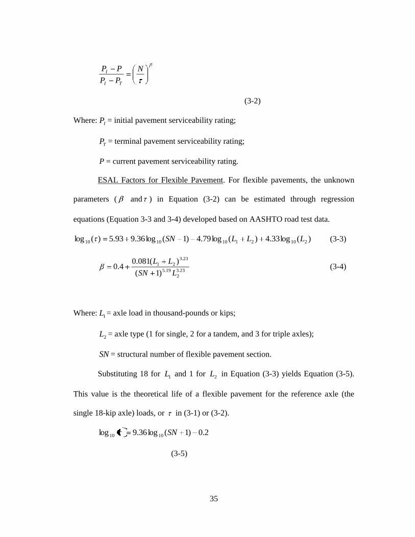
then Equation (3-1) can be rewritten as follows:
35
N
PP
PP
TI
I
(3-2)
Where: IP = initial pavement serviceability rating;
TP = terminal pavement serviceability rating;
P = current pavement serviceability rating.
ESAL Factors for Flexible Pavement. For flexible pavements, the unknown
parameters ( and ) in Equation (3-2) can be estimated through regression
equations (Equation 3-3 and 3-4) developed based on AASHTO road test data.
)(log33.4)(log79.4)1(log36.993.5)(log 21021101010 LLLSN (3-3)
23.3
2
19.5
23.3
21
)1(
)(081.04.0
LSN
LL (3-4)
Where: 1L = axle load in thousand-pounds or kips;
2L = axle type (1 for single, 2 for a tandem, and 3 for triple axles);
SN = structural number of flexible pavement section.
Substituting 18 for 1L and 1 for 2L in Equation (3-3) yields Equation (3-5).
This value is the theoretical life of a flexible pavement for the reference axle (the
single 18-kip axle) loads, or in (3-1) or (3-2).
2.0)1(log36.9log 1010 SN
(3-5)
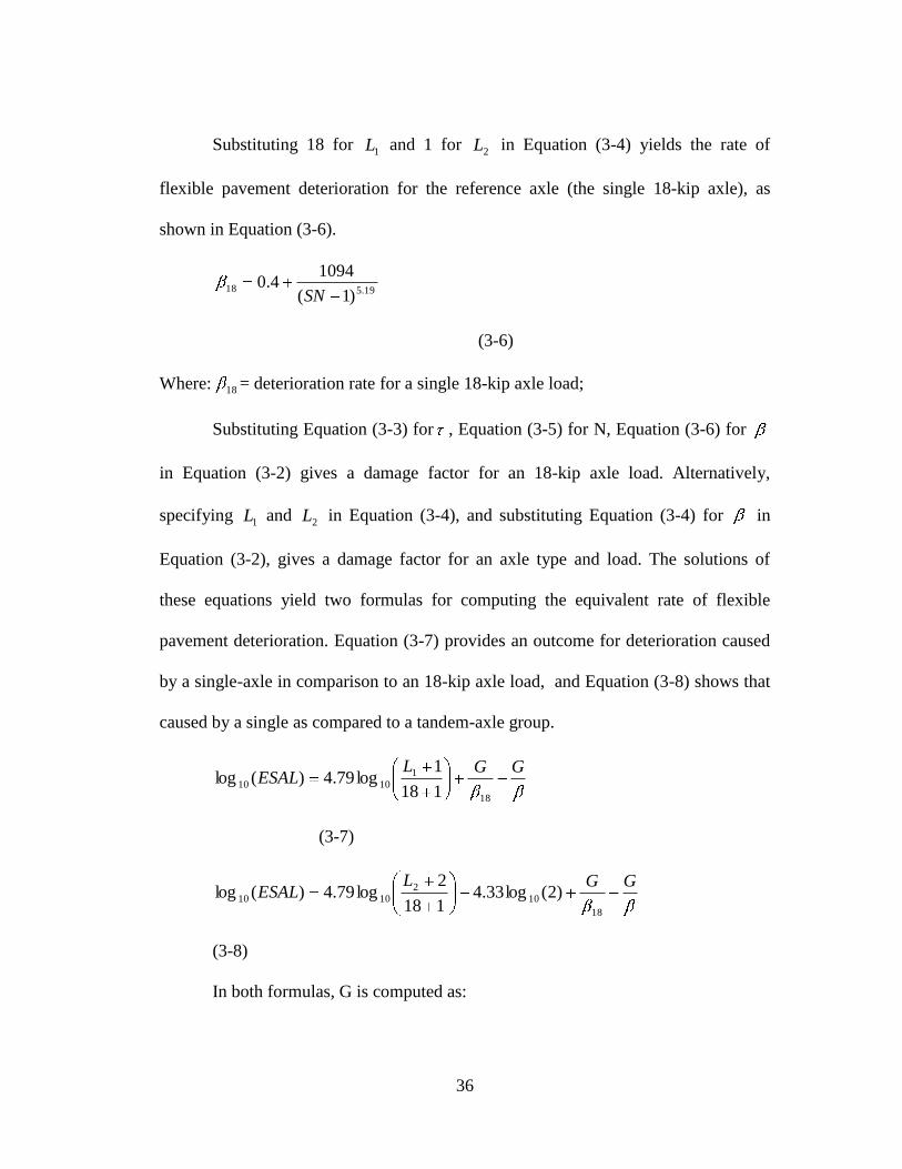
36
Substituting 18 for 1L and 1 for
2L in Equation (3-4) yields the rate of
flexible pavement deterioration for the reference axle (the single 18-kip axle), as
shown in Equation (3-6).
19.518)1(
10944.0
SN
(3-6)
Where: 18 = deterioration rate for a single 18-kip axle load;
Substituting Equation (3-3) for , Equation (3-5) for N, Equation (3-6) for
in Equation (3-2) gives a damage factor for an 18-kip axle load. Alternatively,
specifying 1L and 2L in Equation (3-4), and substituting Equation (3-4) for in
Equation (3-2), gives a damage factor for an axle type and load. The solutions of
these equations yield two formulas for computing the equivalent rate of flexible
pavement deterioration. Equation (3-7) provides an outcome for deterioration caused
by a single-axle in comparison to an 18-kip axle load, and Equation (3-8) shows that
caused by a single as compared to a tandem-axle group.
GGLESAL
18
11010
118
1log79.4)(log
(3-7)
GGLESAL
18
102
1010 )2(log33.4118
2log79.4)(log
(3-8)
In both formulas, G is computed as:
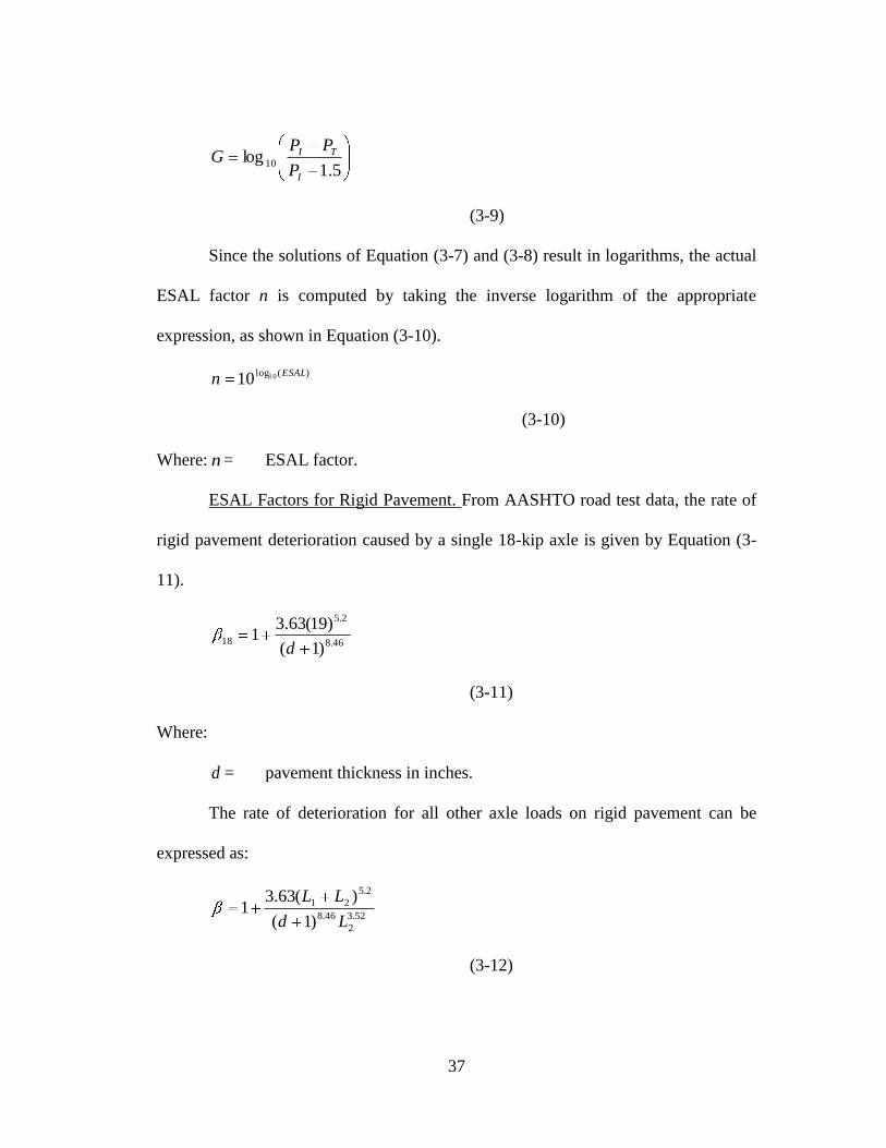
37
5.1log 10
I
TI
P
PPG
(3-9)
Since the solutions of Equation (3-7) and (3-8) result in logarithms, the actual
ESAL factor n is computed by taking the inverse logarithm of the appropriate
expression, as shown in Equation (3-10).
)(log1010ESAL
n
(3-10)
Where: n = ESAL factor.
ESAL Factors for Rigid Pavement. From AASHTO road test data, the rate of
rigid pavement deterioration caused by a single 18-kip axle is given by Equation (3-
11).
46.8
2.5
18)1(
)19(63.31
d
(3-11)
Where:
d = pavement thickness in inches.
The rate of deterioration for all other axle loads on rigid pavement can be
expressed as:
52.3
2
46.8
2.5
21
)1(
)(63.31
Ld
LL
(3-12)
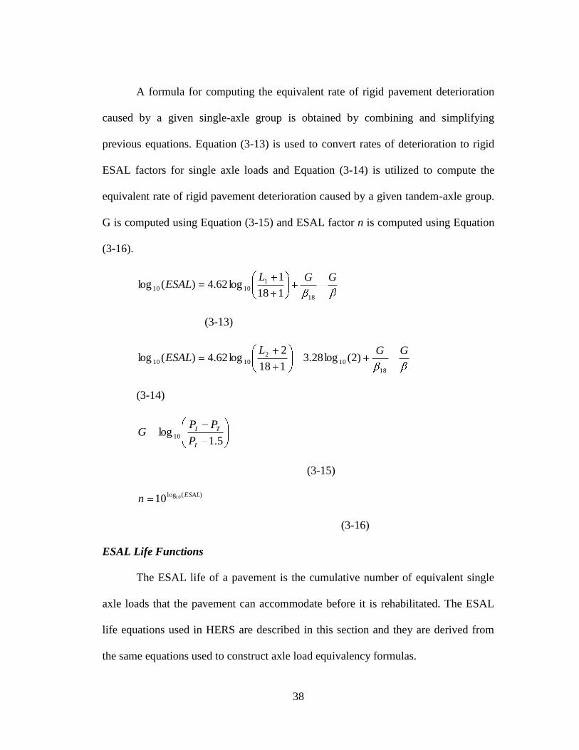
38
A formula for computing the equivalent rate of rigid pavement deterioration
caused by a given single-axle group is obtained by combining and simplifying
previous equations. Equation (3-13) is used to convert rates of deterioration to rigid
ESAL factors for single axle loads and Equation (3-14) is utilized to compute the
equivalent rate of rigid pavement deterioration caused by a given tandem-axle group.
G is computed using Equation (3-15) and ESAL factor n is computed using Equation
(3-16).
GGLESAL
18
11010
118
1log62.4)(log
(3-13)
GGLESAL
18
102
1010 )2(log28.3118
2log62.4)(log
(3-14)
5.1log 10
I
TI
P
PPG
(3-15)
)(log1010ESAL
n
(3-16)
ESAL Life Functions
The ESAL life of a pavement is the cumulative number of equivalent single
axle loads that the pavement can accommodate before it is rehabilitated. The ESAL
life equations used in HERS are described in this section and they are derived from
the same equations used to construct axle load equivalency formulas.
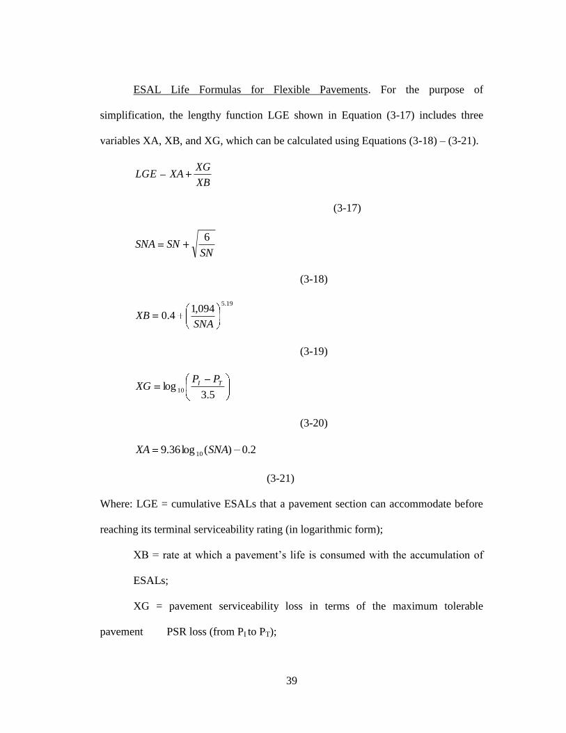
39
ESAL Life Formulas for Flexible Pavements. For the purpose of
simplification, the lengthy function LGE shown in Equation (3-17) includes three
variables XA, XB, and XG, which can be calculated using Equations (3-18) – (3-21).
XB
XGXALGE
(3-17)
SNSNSNA
6
(3-18)
19.5094,1
4.0SNA
XB
(3-19)
5.3log 10
TI PPXG
(3-20)
2.0)(log36.9 10 SNAXA
(3-21)
Where: LGE = cumulative ESALs that a pavement section can accommodate before
reaching its terminal serviceability rating (in logarithmic form);
XB = rate at which a pavement‘s life is consumed with the accumulation of
ESALs;
XG = pavement serviceability loss in terms of the maximum tolerable
pavement PSR loss (from PI to PT);
40
XA = theoretical life of newly constructed pavement in ESALs;
SN = structural number of flexible pavement;
SNA = converted pavement structural number.
Finally, the actual lifecycle of a flexible pavement is computed by taking the
inverse logarithm of LGE:
LGEcleESALlifecy 10
(3-22)
Equation (3-22) shows that the theoretical life of a pavement is directly related
to pavement strength or structural number. However, the rate of pavement decay is
inversely related to strength, as shown in Equation (3-19). Intuitively, both
relationships make sense. In reality, pavements are frequently restored or rehabilitated
before their PSR values decline to the terminal values. Consequently, their theoretical
lives are rarely realized. In such instances, the solution of XG is negative and the ratio
XG/XB adjusts the predicted ESAL life downward from its theoretical maximum. For
example, the predicted ESAL life of a flexible pavement with an SN of 5.3 is
approximately 21 million when the PSR is allowed to decline from 5.0 to 1.5, but
only 10.4 million when the terminal PSR is 2.5.
ESAL Life Formulas for Rigid Pavements. The theoretical life of a rigid
pavement is a function of the thickness of the concrete slab (d).
06.0)1(log35.7 10 dXA
(3-23)
41
46.8)1(
000,240,161
dXB
(3-24)
5.3
)(log 10
TI PPXG
(3-25)
XB
XGXALGE
(3-26)
LGEcleESALlifecy 10
(3-27)
3.2.2 Time-Related Deterioration of Pavements
A pavement will deteriorate over time due to environmental factors in the
absence of truck traffic. Thermal cracking, differential heaving due to swelling
subgrade or frost penetration, disintegration of surface materials due to freeze-thaw
cycles, and other climatic/aging effects on materials are largely a function of the
environment and will result in a loss of pavement serviceability. Figure 3.1 depicts a
likely form for the negative exponential function. This function suggests that
pavement condition declines rapidly when initially exposed to the environmental
elements, but then deteriorates at a decreasing rate over time. This type of decay
process is similar to other natural and man-made phenomena, not just highways.
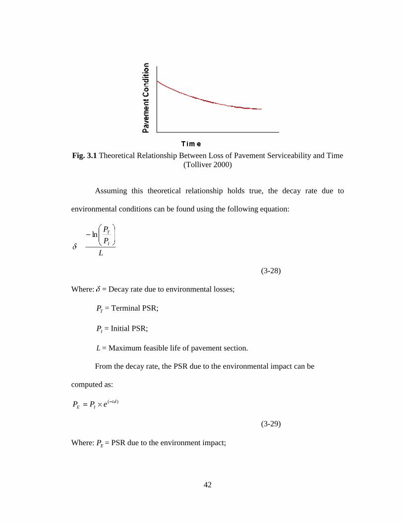
42
Fig. 3.1 Theoretical Relationship Between Loss of Pavement Serviceability and Time
(Tolliver 2000)
Assuming this theoretical relationship holds true, the decay rate due to
environmental conditions can be found using the following equation:
L
P
P
I
Tln
(3-28)
Where: = Decay rate due to environmental losses;
TP = Terminal PSR;
IP = Initial PSR;
L = Maximum feasible life of pavement section.
From the decay rate, the PSR due to the environmental impact can be
computed as:
)( t
IE ePP
(3-29)
Where: EP = PSR due to the environment impact;
43
t = Typical pavement performance period.
3.2.3 Calculation of Structural Numbers
For flexible pavements, the structural number can be determined using
Equation (3-30).
3322
*
1
*
111 dadadadaSN
(3-30)
Where: 1d Thickness of surface layer (inches);
1a Surface layer coefficient;
*
1d Thickness of old surface layer as a base course (inches);
*
1a Layer coefficient of old surface layer;
2d Thickness of base (inches);
2a Base layer coefficient;
3d Thickness of subbase (inches);
3a Subbase layer coefficient.
In this study, the data of pavement structure and depth of each pavement layer
were collected from KDOT‘s Pavement Management Information System (PMIS).
The layer coefficients shown in the Table 3.1 were used to compute structural
numbers, as shown in Equation (3-30).
Table 3.1 Layer Coefficients Used to Compute Pavement Structural Numbers
(Tolliver 2000)
Material Layer Description Layer
Coefficient
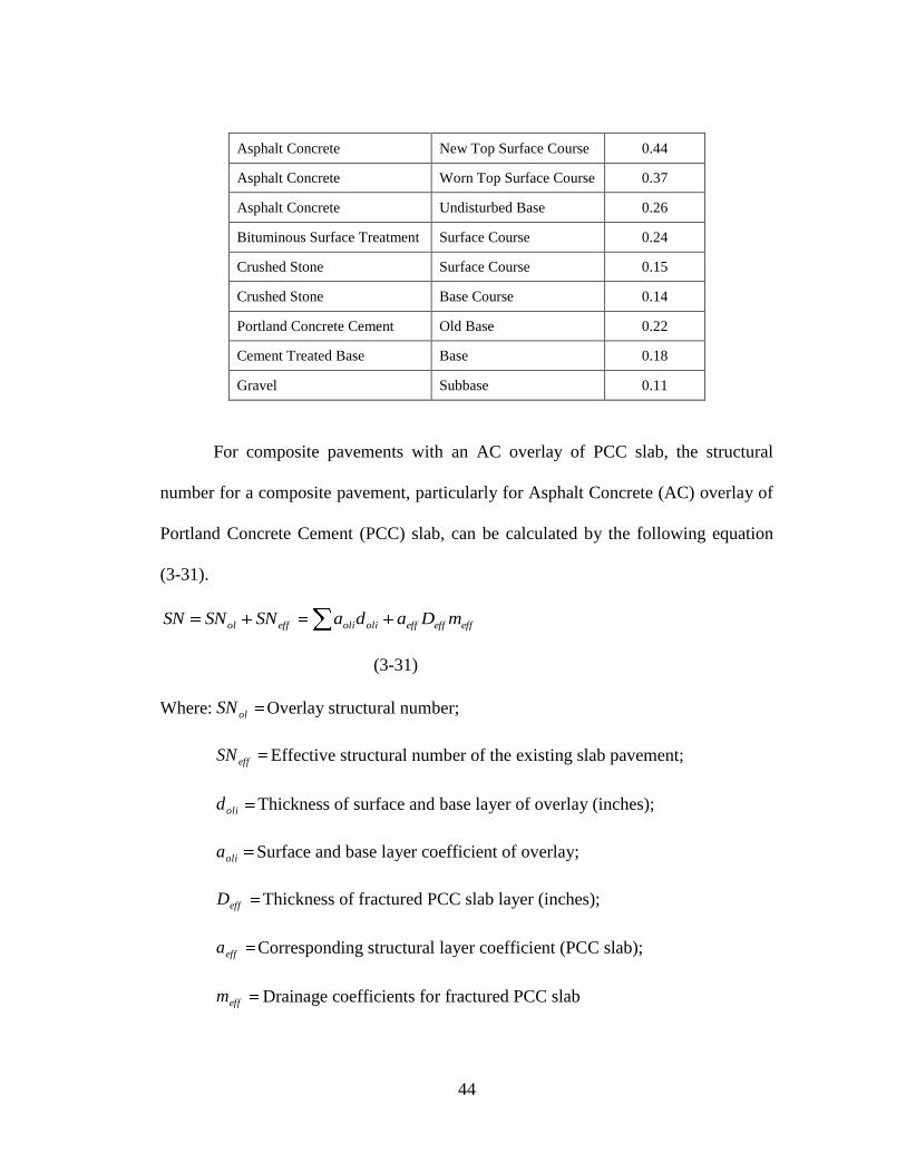
44
Asphalt Concrete New Top Surface Course 0.44
Asphalt Concrete Worn Top Surface Course 0.37
Asphalt Concrete Undisturbed Base 0.26
Bituminous Surface Treatment Surface Course 0.24
Crushed Stone Surface Course 0.15
Crushed Stone Base Course 0.14
Portland Concrete Cement Old Base 0.22
Cement Treated Base Base 0.18
Gravel Subbase 0.11
For composite pavements with an AC overlay of PCC slab, the structural
number for a composite pavement, particularly for Asphalt Concrete (AC) overlay of
Portland Concrete Cement (PCC) slab, can be calculated by the following equation
(3-31).
effeffeffoliolieffol mDadaSNSNSN
(3-31)
Where: olSN Overlay structural number;
effSN Effective structural number of the existing slab pavement;
olid Thickness of surface and base layer of overlay (inches);
olia Surface and base layer coefficient of overlay;
effD Thickness of fractured PCC slab layer (inches);
effa Corresponding structural layer coefficient (PCC slab);
effm Drainage coefficients for fractured PCC slab
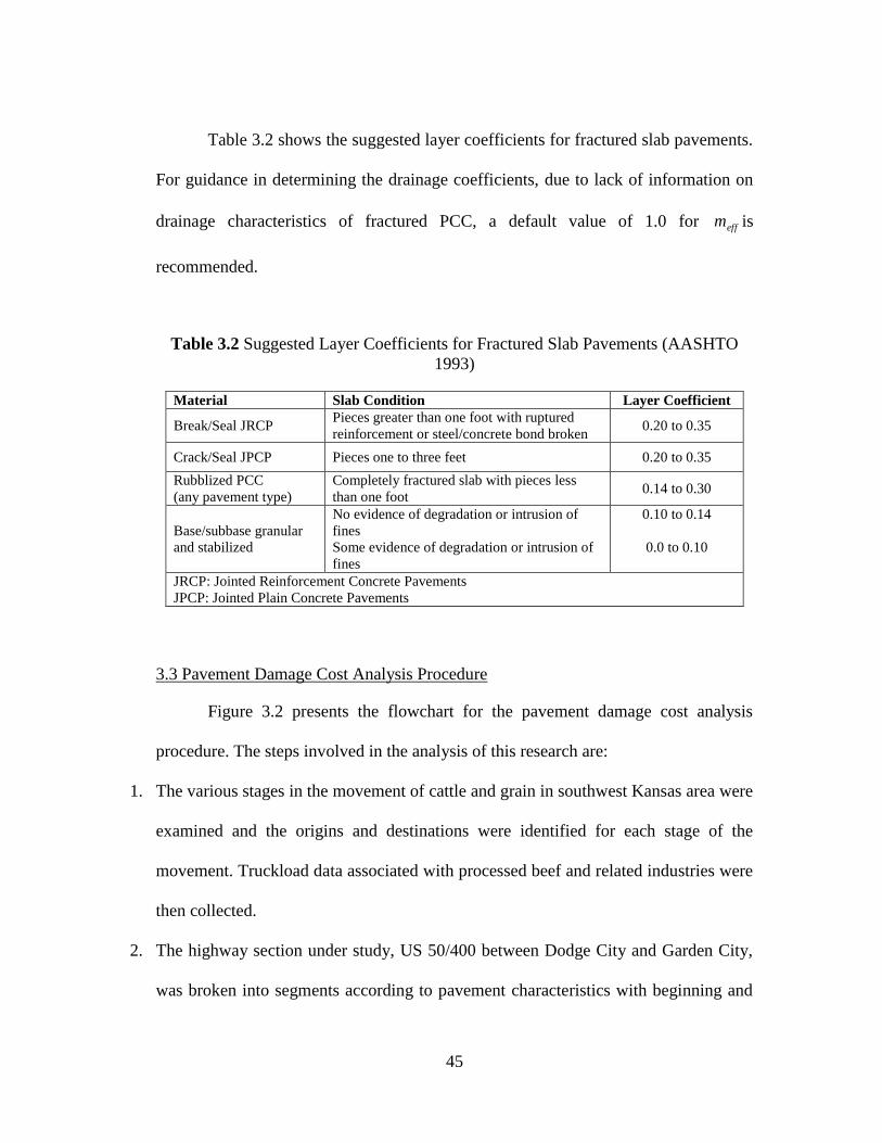
45
Table 3.2 shows the suggested layer coefficients for fractured slab pavements.
For guidance in determining the drainage coefficients, due to lack of information on
drainage characteristics of fractured PCC, a default value of 1.0 for effm is
recommended.
Table 3.2 Suggested Layer Coefficients for Fractured Slab Pavements (AASHTO
1993)
Material Slab Condition Layer Coefficient
Break/Seal JRCP Pieces greater than one foot with ruptured
reinforcement or steel/concrete bond broken 0.20 to 0.35
Crack/Seal JPCP Pieces one to three feet 0.20 to 0.35
Rubblized PCC
(any pavement type)
Completely fractured slab with pieces less
than one foot 0.14 to 0.30
Base/subbase granular
and stabilized
No evidence of degradation or intrusion of
fines
Some evidence of degradation or intrusion of
fines
0.10 to 0.14
0.0 to 0.10
JRCP: Jointed Reinforcement Concrete Pavements
JPCP: Jointed Plain Concrete Pavements
3.3 Pavement Damage Cost Analysis Procedure
Figure 3.2 presents the flowchart for the pavement damage cost analysis
procedure. The steps involved in the analysis of this research are:
1. The various stages in the movement of cattle and grain in southwest Kansas area were
examined and the origins and destinations were identified for each stage of the
movement. Truckload data associated with processed beef and related industries were
then collected.
2. The highway section under study, US 50/400 between Dodge City and Garden City,
was broken into segments according to pavement characteristics with beginning and
46
ending milepost references. Key highway attributes of each pavement segment were
compiled using KDOT‘s PMIS database, including the functional class, pavement
type, structural number or slab thickness, and design (initial) and terminal PSR. The
truck traffic was estimated and assigned in the southwest Kansas area using
TransCAD software. Based on the identified truck routes and the collected truckload
data, the total truck VMTs associated with processed beef and related industries on
each pavement segment were estimated.
3. ESAL factors were computed for the truck type 3-S2 traveling on each highway
segment.
4. Truck ESAL factors were multiplied by the truck VMTs associated with the
processed beef and related industries to compute annual ESALs for each pavement
segment.
5. The lives of the studied pavement segments in terms of ESALs were determined. In
this step, the ESAL life functions were used to compute the ESAL lives of studied
pavements. The ESAL life is the cumulative number of axle passes that will cause the
PSR of a pavement section to decline from its design level to its terminal
serviceability rating irrespective of the time involved.
6. The maximum life of a pavement segment was defined in terms of a tolerable decline
in PSR. For the studied highway, KDOT designs for an initial PSR at 4.2 and a
terminal PSR at 2.5. Thus, the maximum tolerable decline in PSR is 1.7. In this
research, the maximum feasible life of a pavement segment was determined as 30
years according to KDOT pavement design criteria.
47
7. The loss in PSR from environmental factors was computed using the time-related
deterioration function for a typical design performance period for the studied
pavement segments. Only the remaining pavement rehabilitation costs were
considered because of traffic.
8. Unit costs per ESAL were computed by multiplying the average resurfacing or
reconstruction costs per mile by the percent of PSR loss due to traffic and dividing by
the ESAL lives of the pavement segments. To illustrate the process, assume that a
pavement segment has an ESAL life of 500,000, rehabilitation and reconstruction
cost of $300,000 per mile, and 40% of the pavement deterioration is due to
environmental factors. In this example, the rehabilitation cost due to traffic is
$300,000 x (1-40%)/500,000 = $0.36 per ESAL.
9. The contributed pavement damage cost for the studied highway section was
computed by multiplying the annual ESALs associated with processed beef and
related industries by the average unit cost per ESAL.
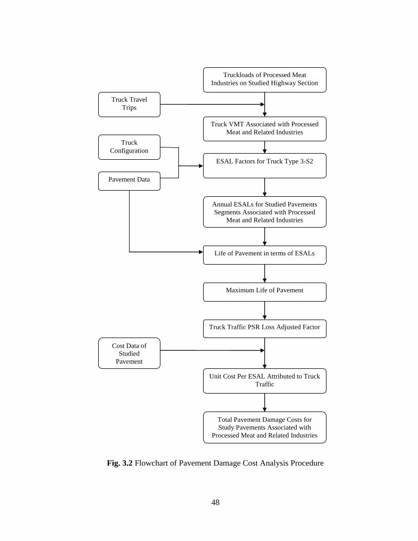
48
Fig. 3.2 Flowchart of Pavement Damage Cost Analysis Procedure
Truckloads of Processed Meat
Industries on Studied Highway Section
Truck Travel
Trips
Truck VMT Associated with Processed
Meat and Related Industries
Pavement Data
Truck
Configuration
ESAL Factors for Truck Type 3-S2
Life of Pavement in terms of ESALs
Truck Traffic PSR Loss Adjusted Factor
Annual ESALs for Studied Pavements
Segments Associated with Processed
Meat and Related Industries
Unit Cost Per ESAL Attributed to Truck
Traffic
Total Pavement Damage Costs for
Study Pavements Associated with
Processed Meat and Related Industries
Cost Data of
Studied
Pavement
Maximum Life of Pavement
49
3.4 Data Input Requirements
The key data required by the calculations included the configuration of trucks
and the pavement information of the highway section under study. It was assumed
that all grain hauling vehicles were type 3-S2 with five-axle semi-tractor trailer
configurations, and loading configurations were assumed to be 10/35/35. The detailed
configurations of this vehicle type can be found in the Comprehensive Truck Size and
Weight Study prepared for the U.S. Department of Transportation (USDOT 2000).
The important pavement data inputs required for this study included:
Structural number for flexible pavement (SN)
Initial PSR ( 0p )
Terminal PSR ( tp )
Maximum feasible life of pavement segment in years (L)
Typical pavement performance ( )
KDOT maintains all the pavement segment data in its PMIS database. In this
research, the required pavement data for the calculations were provided by KDOT.
3.5 Pavement Damage Cost Analysis
The annual pavement damage costs attributed to these VMTs were evaluated
based on the estimated annual total truck VMTs on the studied pavement segments.
The characteristics of the pavement segments were obtained from the KDOT PMIS
database.
Designation as U.S., State, or Interstate highway
Route number
50
Beginning and ending points of highway segments
Pavement type
Length of pavement segment
Pavement structure number
Maintenance activity and cost record
To calculate the pavement damage costs due to trucks for processed beef and
related industries, it was necessary to calculate ESAL factors for typical truck types
and pavement types. In this study, the selected truck model was a 3-S2 tractor-and-
trailer with a loading configuration of 10/35/35. This configuration means that the
tractor unit applies a 10,000 pound load to the front axle, and each of two tandem axle
groups under the trailer supports 35,000 pounds. The maximum legal GVW of the
truck is 80,000 pounds.
The impact of this truck on pavement varies depending on pavement
characteristics. There are three basic steps involved in calculating the ESAL factor.
First, the rate of deterioration was computed for the 18,000-pound reference axle.
Second, the deterioration rates of the interest axle loads were computed. Finally, the
two deterioration rates were used to compute the ESAL factors. These computations
required the knowledge of the type of axle group, the load in kips, the initial and
terminal PSR, pavement characteristics and type. As mentioned earlier, the four
pavement segments on the studied highway section, US 50/400 between Garden City
and Dodge City, were considered as flexible pavements during the calculation of
pavement damage. The only exception being the calculation of the structural numbers
51
in which equations for composite pavements were used when available. The
following sections describe the pavement damage computation procedure and
corresponding results.
3.5.1 Calculation of ESAL Factors and Annual ESALs
Pavement structural numbers are key inputs for the calculation of ESAL
factors. The numbers for pavement segments 1 and 2 were obtained directly from
KDOT PMIS system as 5.4 and 3.05. On the other hand, the structure numbers for
segments 3 and 4 had to be computed based on their pavement structure information.
Pavement segment 3 had the surface layer of 40 mm (1.57 in) BM-1T and the base
course was the original layers with a total thickness of 330 mm (13.0 in). In Kansas,
KDOT designs full depth asphalt pavements without a base layer. The subbase layer
is the subgrade—the natural soil. Equation (3-30) was used to determine the SN for
PS 3. The layer coefficients 1a and
*
1a were selected from Table 5.1 as 0.4 and 0.26,
respectively. Therefore, the SN for segment 3 was calculated as follows:
SN (PS 3) = 0.426.00.134.057.1
PS 4 is a composite pavement segment which has a surface layer of 38 mm
(1.5 in) BM-1T, a 151 mm (5.95 in) base course of HMA (Hot Mix Asphalt), and a
178 mm (7.01 in) subbase layer of Concrete Pavement on the subgrade (natural soil).
Based on Table 5.2, the layer coefficients 1oa , *
01a and effa were selected as 0.4, 0.26
and 0.22, respectively. Equation (3-31) was used to compute SN for PS 4:
SN (PS 4) = 69.322.001.7)26.095.54.05.1(
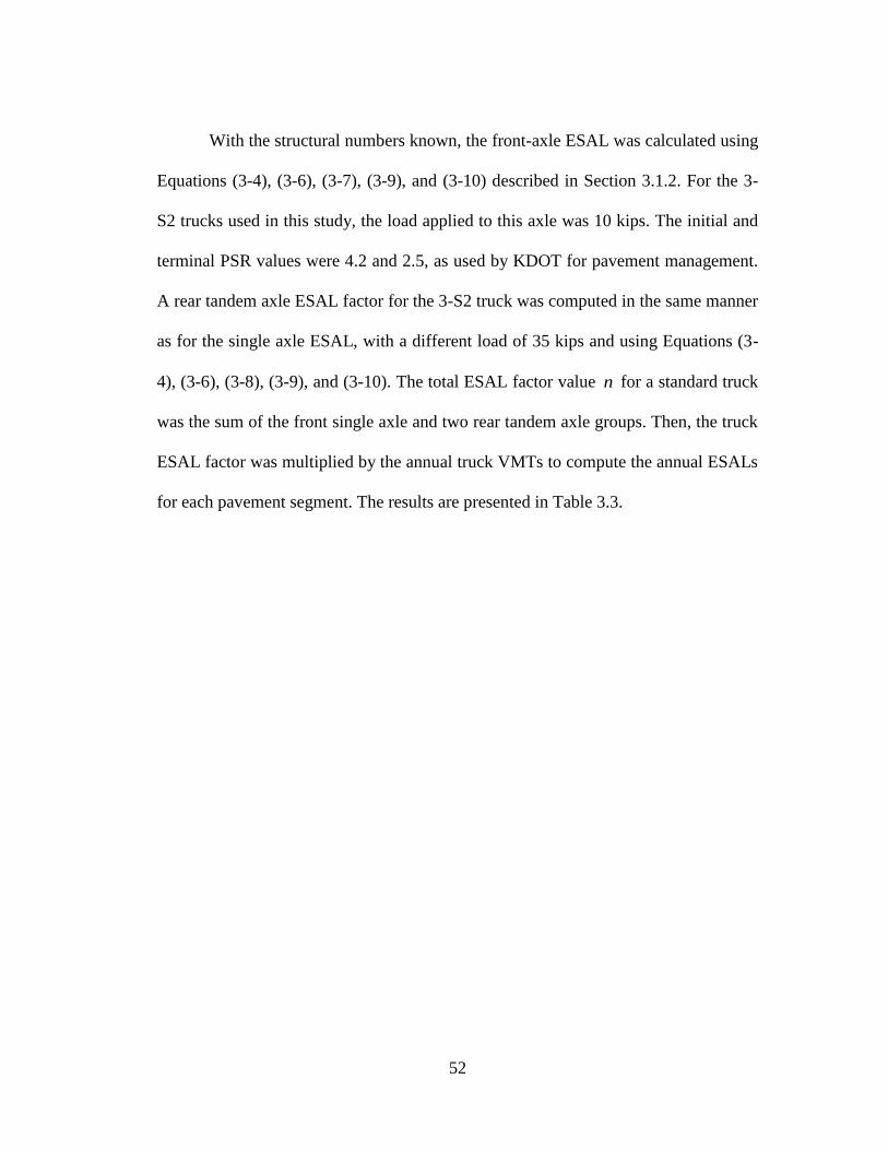
52
With the structural numbers known, the front-axle ESAL was calculated using
Equations (3-4), (3-6), (3-7), (3-9), and (3-10) described in Section 3.1.2. For the 3-
S2 trucks used in this study, the load applied to this axle was 10 kips. The initial and
terminal PSR values were 4.2 and 2.5, as used by KDOT for pavement management.
A rear tandem axle ESAL factor for the 3-S2 truck was computed in the same manner
as for the single axle ESAL, with a different load of 35 kips and using Equations (3-
4), (3-6), (3-8), (3-9), and (3-10). The total ESAL factor value n for a standard truck
was the sum of the front single axle and two rear tandem axle groups. Then, the truck
ESAL factor was multiplied by the annual truck VMTs to compute the annual ESALs
for each pavement segment. The results are presented in Table 3.3.
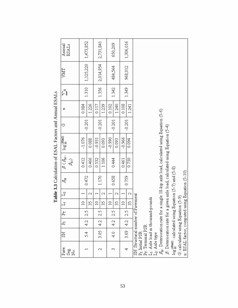
53
Tab
le 3
.3 C
alcu
lati
on o
f E
SA
L F
acto
rs a
nd A
nnu
al E
SA
Ls
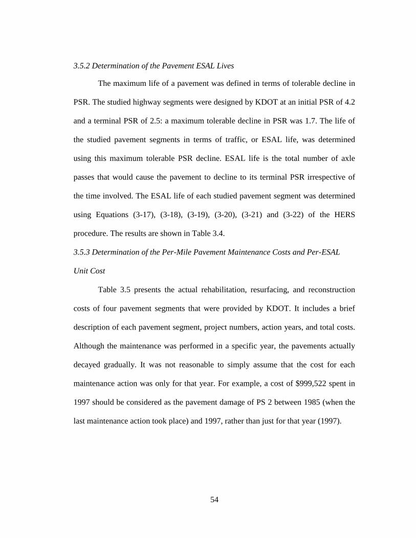
54
3.5.2 Determination of the Pavement ESAL Lives
The maximum life of a pavement was defined in terms of tolerable decline in
PSR. The studied highway segments were designed by KDOT at an initial PSR of 4.2
and a terminal PSR of 2.5: a maximum tolerable decline in PSR was 1.7. The life of
the studied pavement segments in terms of traffic, or ESAL life, was determined
using this maximum tolerable PSR decline. ESAL life is the total number of axle
passes that would cause the pavement to decline to its terminal PSR irrespective of
the time involved. The ESAL life of each studied pavement segment was determined
using Equations (3-17), (3-18), (3-19), (3-20), (3-21) and (3-22) of the HERS
procedure. The results are shown in Table 3.4.
3.5.3 Determination of the Per-Mile Pavement Maintenance Costs and Per-ESAL
Unit Cost
Table 3.5 presents the actual rehabilitation, resurfacing, and reconstruction
costs of four pavement segments that were provided by KDOT. It includes a brief
description of each pavement segment, project numbers, action years, and total costs.
Although the maintenance was performed in a specific year, the pavements actually
decayed gradually. It was not reasonable to simply assume that the cost for each
maintenance action was only for that year. For example, a cost of $999,522 spent in
1997 should be considered as the pavement damage of PS 2 between 1985 (when the
last maintenance action took place) and 1997, rather than just for that year (1997).
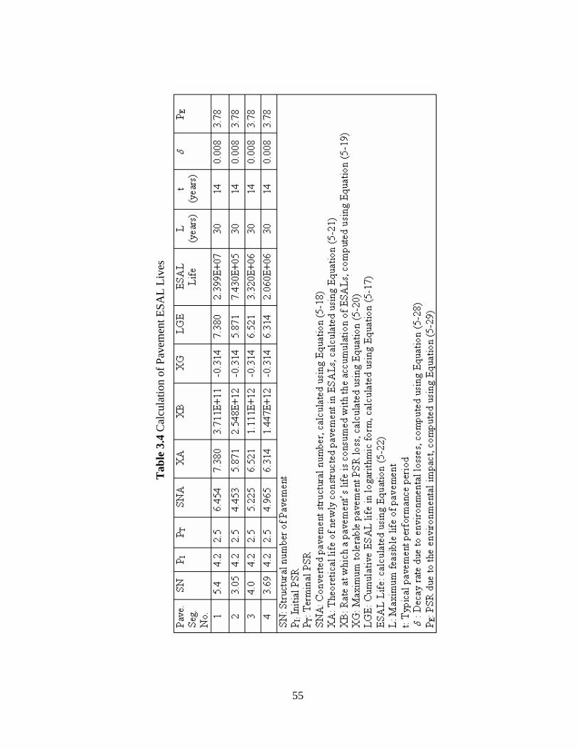
55
Tab
le 3
.4 C
alcu
lati
on o
f P
avem
ent
ES
AL
Liv
es
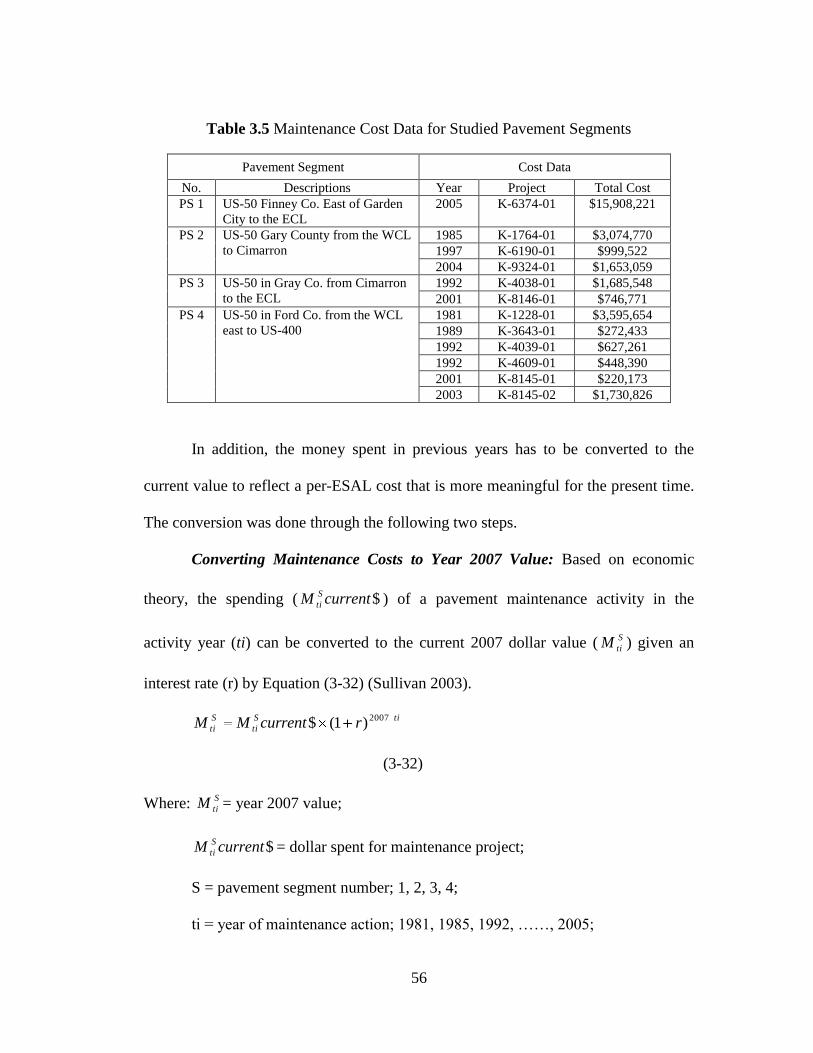
56
Table 3.5 Maintenance Cost Data for Studied Pavement Segments
Pavement Segment Cost Data
No. Descriptions Year Project Total Cost
PS 1 US-50 Finney Co. East of Garden
City to the ECL
2005 K-6374-01 $15,908,221
PS 2 US-50 Gary County from the WCL
to Cimarron
1985 K-1764-01 $3,074,770
1997 K-6190-01 $999,522
2004 K-9324-01 $1,653,059
PS 3 US-50 in Gray Co. from Cimarron
to the ECL
1992 K-4038-01 $1,685,548
2001 K-8146-01 $746,771
PS 4 US-50 in Ford Co. from the WCL
east to US-400
1981 K-1228-01 $3,595,654
1989 K-3643-01 $272,433
1992 K-4039-01 $627,261
1992 K-4609-01 $448,390
2001 K-8145-01 $220,173
2003 K-8145-02 $1,730,826
In addition, the money spent in previous years has to be converted to the
current value to reflect a per-ESAL cost that is more meaningful for the present time.
The conversion was done through the following two steps.
Converting Maintenance Costs to Year 2007 Value: Based on economic
theory, the spending ( $currentM S
ti ) of a pavement maintenance activity in the
activity year (ti) can be converted to the current 2007 dollar value (S
tiM ) given an
interest rate (r) by Equation (3-32) (Sullivan 2003).
tiS
ti
S
ti rcurrentMM 2007)1($
(3-32)
Where: S
tiM = year 2007 value;
$currentM S
ti = dollar spent for maintenance project;
S = pavement segment number; 1, 2, 3, 4;
ti = year of maintenance action; 1981, 1985, 1992, ……, 2005;
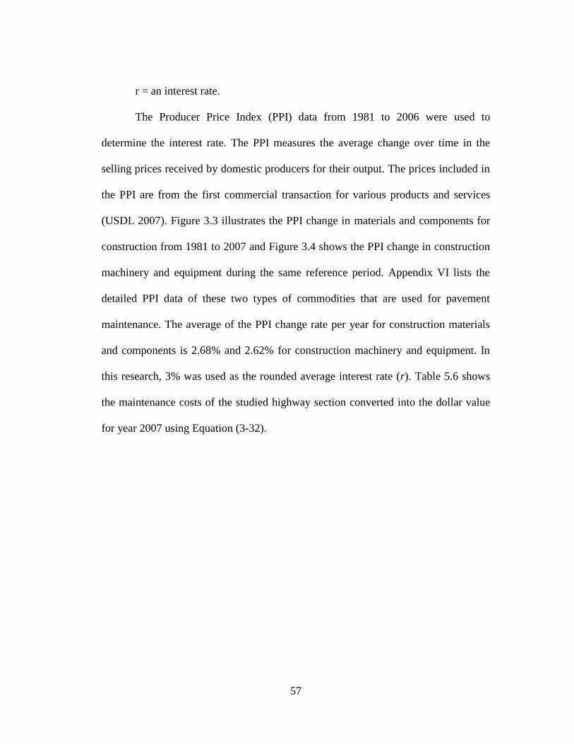
57
r = an interest rate.
The Producer Price Index (PPI) data from 1981 to 2006 were used to
determine the interest rate. The PPI measures the average change over time in the
selling prices received by domestic producers for their output. The prices included in
the PPI are from the first commercial transaction for various products and services
(USDL 2007). Figure 3.3 illustrates the PPI change in materials and components for
construction from 1981 to 2007 and Figure 3.4 shows the PPI change in construction
machinery and equipment during the same reference period. Appendix VI lists the
detailed PPI data of these two types of commodities that are used for pavement
maintenance. The average of the PPI change rate per year for construction materials
and components is 2.68% and 2.62% for construction machinery and equipment. In
this research, 3% was used as the rounded average interest rate (r). Table 5.6 shows
the maintenance costs of the studied highway section converted into the dollar value
for year 2007 using Equation (3-32).

58
Fig. 3.3 PPI Change in Materials and Components for Construction from 1981 to
2007 (USDL 2007)
Fig. 3.4 PPI Change in Construction Machinery and Equipment from 1981 to 2007
(USDL 2007)
Year
Year
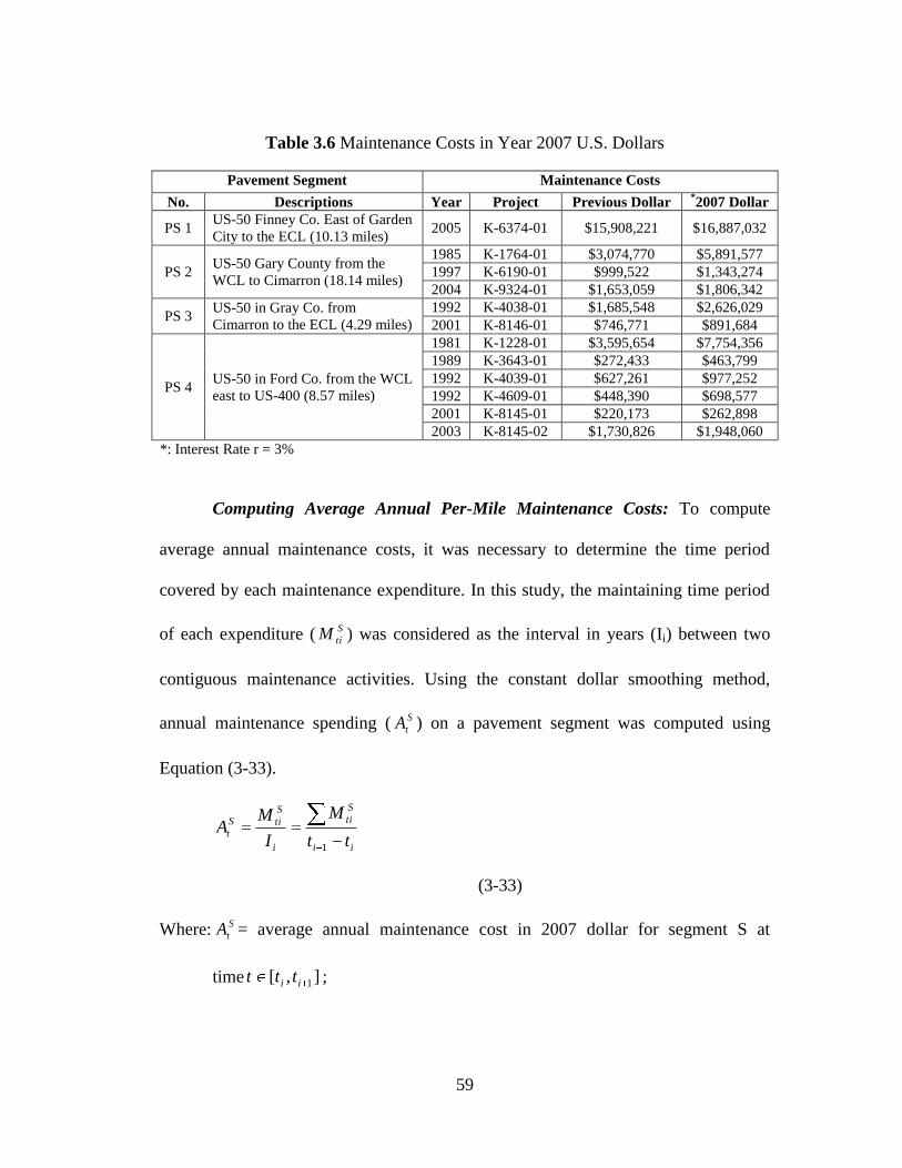
59
Table 3.6 Maintenance Costs in Year 2007 U.S. Dollars
Pavement Segment Maintenance Costs
No. Descriptions Year Project Previous Dollar *2007 Dollar
PS 1 US-50 Finney Co. East of Garden
City to the ECL (10.13 miles) 2005 K-6374-01 $15,908,221 $16,887,032
PS 2 US-50 Gary County from the
WCL to Cimarron (18.14 miles)
1985 K-1764-01 $3,074,770 $5,891,577
1997 K-6190-01 $999,522 $1,343,274
2004 K-9324-01 $1,653,059 $1,806,342
PS 3 US-50 in Gray Co. from
Cimarron to the ECL (4.29 miles)
1992 K-4038-01 $1,685,548 $2,626,029
2001 K-8146-01 $746,771 $891,684
PS 4 US-50 in Ford Co. from the WCL
east to US-400 (8.57 miles)
1981 K-1228-01 $3,595,654 $7,754,356
1989 K-3643-01 $272,433 $463,799
1992 K-4039-01 $627,261 $977,252
1992 K-4609-01 $448,390 $698,577
2001 K-8145-01 $220,173 $262,898
2003 K-8145-02 $1,730,826 $1,948,060
*: Interest Rate r = 3%
Computing Average Annual Per-Mile Maintenance Costs: To compute
average annual maintenance costs, it was necessary to determine the time period
covered by each maintenance expenditure. In this study, the maintaining time period
of each expenditure (S
tiM ) was considered as the interval in years (Ii) between two
contiguous maintenance activities. Using the constant dollar smoothing method,
annual maintenance spending (S
tA ) on a pavement segment was computed using
Equation (3-33).
ii
S
ti
i
S
tiS
ttt
M
I
MA
1
(3-33)
Where: S
tA = average annual maintenance cost in 2007 dollar for segment S at
time ],[ 1ii ttt ;
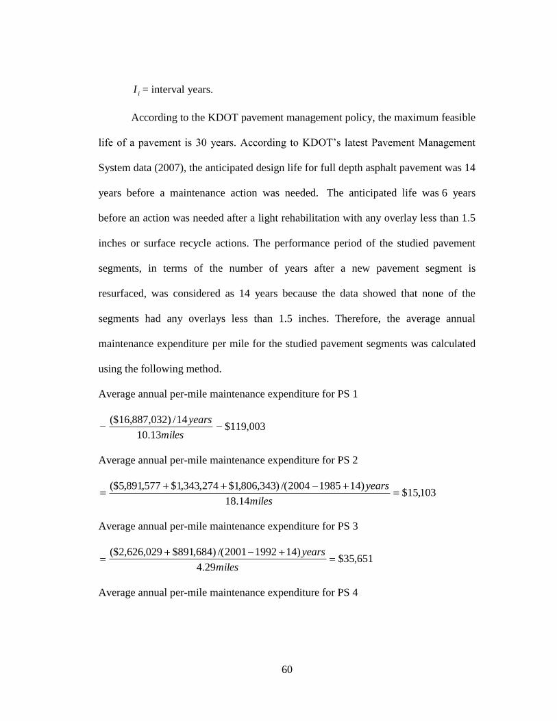
60
iI = interval years.
According to the KDOT pavement management policy, the maximum feasible
life of a pavement is 30 years. According to KDOT‘s latest Pavement Management
System data (2007), the anticipated design life for full depth asphalt pavement was 14
years before a maintenance action was needed. The anticipated life was 6 years
before an action was needed after a light rehabilitation with any overlay less than 1.5
inches or surface recycle actions. The performance period of the studied pavement
segments, in terms of the number of years after a new pavement segment is
resurfaced, was considered as 14 years because the data showed that none of the
segments had any overlays less than 1.5 inches. Therefore, the average annual
maintenance expenditure per mile for the studied pavement segments was calculated
using the following method.
Average annual per-mile maintenance expenditure for PS 1
003,119$13.10
14/)032,887,16($
miles
years
Average annual per-mile maintenance expenditure for PS 2
103,15$14.18
)1419852004/()343,806,1$274,343,1$577,891,5($
miles
years
Average annual per-mile maintenance expenditure for PS 3
651,35$29.4
)1419922001/()684,891$029,626,2($
miles
years
Average annual per-mile maintenance expenditure for PS 4
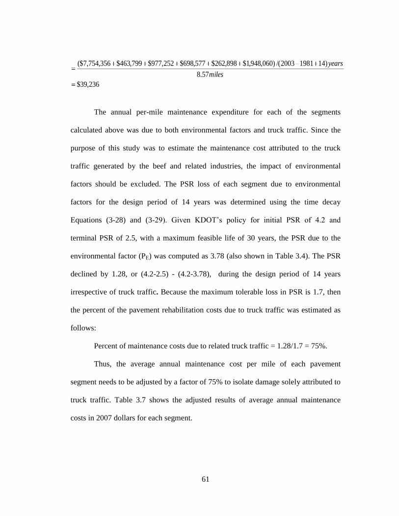
61
236,39$
57.8
)1419812003/()060,948,1$898,262$577,698$252,977$799,463$356,754,7($
miles
years
The annual per-mile maintenance expenditure for each of the segments
calculated above was due to both environmental factors and truck traffic. Since the
purpose of this study was to estimate the maintenance cost attributed to the truck
traffic generated by the beef and related industries, the impact of environmental
factors should be excluded. The PSR loss of each segment due to environmental
factors for the design period of 14 years was determined using the time decay
Equations (3-28) and (3-29). Given KDOT‘s policy for initial PSR of 4.2 and
terminal PSR of 2.5, with a maximum feasible life of 30 years, the PSR due to the
environmental factor (PE) was computed as 3.78 (also shown in Table 3.4). The PSR
declined by 1.28, or (4.2-2.5) - (4.2-3.78), during the design period of 14 years
irrespective of truck traffic. Because the maximum tolerable loss in PSR is 1.7, then
the percent of the pavement rehabilitation costs due to truck traffic was estimated as
follows:
Percent of maintenance costs due to related truck traffic = 1.28/1.7 = 75%.
Thus, the average annual maintenance cost per mile of each pavement
segment needs to be adjusted by a factor of 75% to isolate damage solely attributed to
truck traffic. Table 3.7 shows the adjusted results of average annual maintenance
costs in 2007 dollars for each segment.
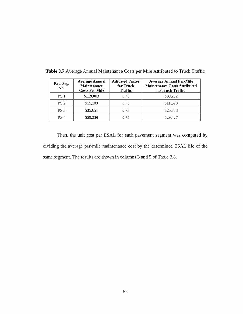
62
Table 3.7 Average Annual Maintenance Costs per Mile Attributed to Truck Traffic
Pav. Seg.
No.
Average Annual
Maintenance
Costs Per Mile
Adjusted Factor
for Truck
Traffic
Average Annual Per-Mile
Maintenance Costs Attributed
to Truck Traffic
PS 1 $119,003 0.75 $89,252
PS 2 $15,103 0.75 $11,328
PS 3 $35,651 0.75 $26,738
PS 4 $39,236 0.75 $29,427
Then, the unit cost per ESAL for each pavement segment was computed by
dividing the average per-mile maintenance cost by the determined ESAL life of the
same segment. The results are shown in columns 3 and 5 of Table 3.8.
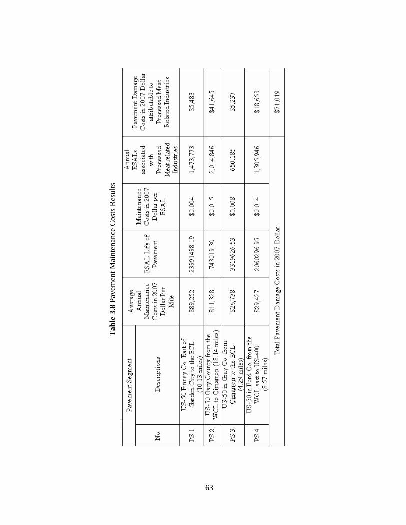
63
Tab
le 3
.8 P
avem
ent
Mai
nte
nan
ce C
ost
s R
esult
s
64
3.5.4 Damage Costs Attributed to Beef and Related Industries
As mentioned in previous sections, the values of the parameters used in the
pavement damage analysis for the four pavement segments and the calculation results
are summarized in Tables 3.3 and 3.4. The damage cost for each of the studied
pavement segments was estimated as the unit cost per ESAL multiplied by the annual
ESALs on each segment. The results are presented in the last column of Table 3.8.
After summing costs from four pavement segments, the result represents the annual
pavement damage costs on the studied highway section attributed to processed beef
and related industries in southwest Kansas.
In summary, for the 41.13 miles on US 50/400 between Garden City and
Dodge City, the total annual highway damage associated with processed meat and
related industries in southwest Kansas was estimated at $71,019, or $1,727 per mile.
The annual damage cost per truck per mile was approximately $0.02. Table 3.9 lists
the pavement length of major highways in the southwest Kansas region. If the same
truck traffic were to be present on all these major highways in southwest Kansas
(approximately 1835 miles), the total annual damage costs attributed to processed
meat and related industries would be $3,169,045.
The meat processing industry, especially for boxed beef and byproducts, is
expected to grow 13% from 2007 to 2015 nationwide. For feed yards, the growth of
feeder cattle will be proportional to the industry growth. Some researchers projected
that the number of cattle could even triple by then. In addition, related industries,
such as dairy, are projected to grow significantly. Overall, the truck volumes
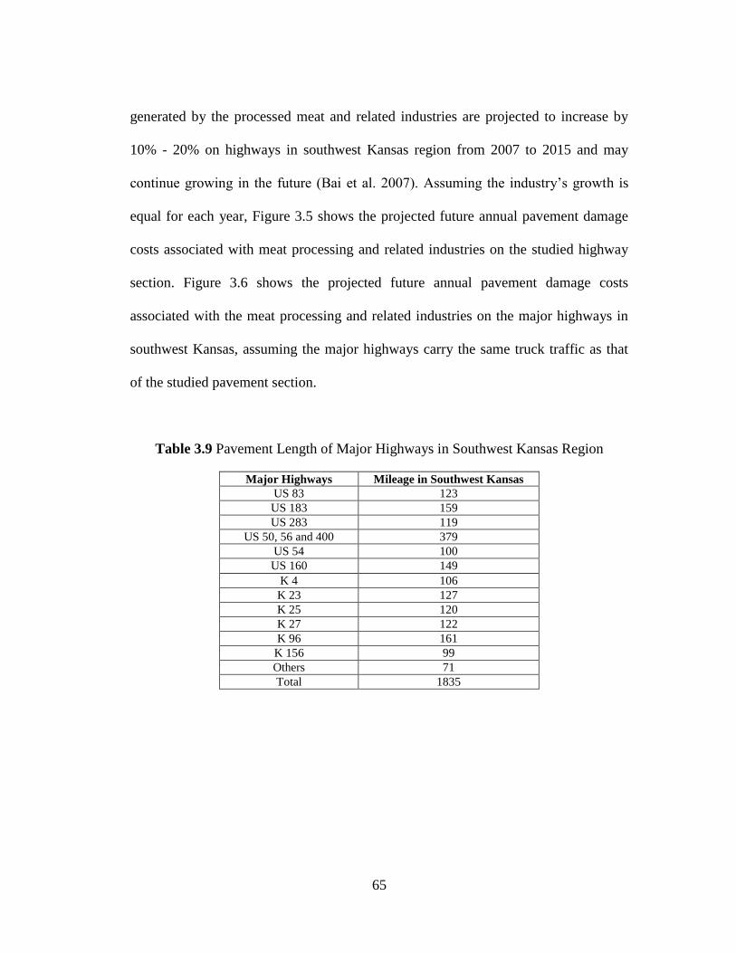
65
generated by the processed meat and related industries are projected to increase by
10% - 20% on highways in southwest Kansas region from 2007 to 2015 and may
continue growing in the future (Bai et al. 2007). Assuming the industry‘s growth is
equal for each year, Figure 3.5 shows the projected future annual pavement damage
costs associated with meat processing and related industries on the studied highway
section. Figure 3.6 shows the projected future annual pavement damage costs
associated with the meat processing and related industries on the major highways in
southwest Kansas, assuming the major highways carry the same truck traffic as that
of the studied pavement section.
Table 3.9 Pavement Length of Major Highways in Southwest Kansas Region
Major Highways Mileage in Southwest Kansas
US 83 123
US 183 159
US 283 119
US 50, 56 and 400 379
US 54 100
US 160 149
K 4 106
K 23 127
K 25 120
K 27 122
K 96 161
K 156 99
Others 71
Total 1835
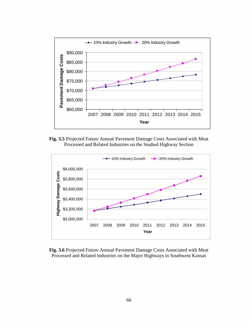
66
Fig. 3.5 Projected Future Annual Pavement Damage Costs Associated with Meat
Processed and Related Industries on the Studied Highway Section
Fig. 3.6 Projected Future Annual Pavement Damage Costs Associated with Meat
Processed and Related Industries on the Major Highways in Southwest Kansas
$60,000
$65,000
$70,000
$75,000
$80,000
$85,000
$90,000
2007 2008 2009 2010 2011 2012 2013 2014 2015
Year
Pa
ve
me
nt
Da
ma
ge
Co
sts
10% Industry Growth 20% Industry Growth
$3,000,000
$3,200,000
$3,400,000
$3,600,000
$3,800,000
$4,000,000
2007 2008 2009 2010 2011 2012 2013 2014 2015
Hig
hw
ay D
am
ag
e C
os
ts
Year
10% Industry Growth 20% Industry Growth
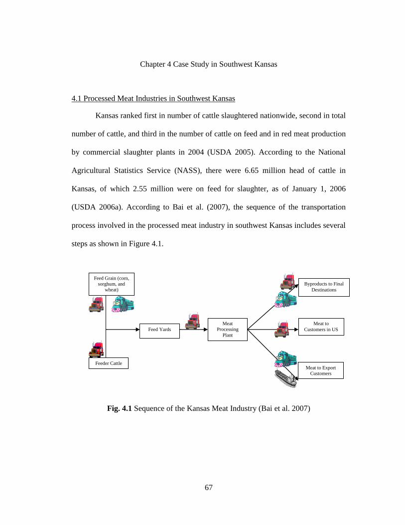
67
Chapter 4 Case Study in Southwest Kansas
4.1 Processed Meat Industries in Southwest Kansas
Kansas ranked first in number of cattle slaughtered nationwide, second in total
number of cattle, and third in the number of cattle on feed and in red meat production
by commercial slaughter plants in 2004 (USDA 2005). According to the National
Agricultural Statistics Service (NASS), there were 6.65 million head of cattle in
Kansas, of which 2.55 million were on feed for slaughter, as of January 1, 2006
(USDA 2006a). According to Bai et al. (2007), the sequence of the transportation
process involved in the processed meat industry in southwest Kansas includes several
steps as shown in Figure 4.1.
Fig. 4.1 Sequence of the Kansas Meat Industry (Bai et al. 2007)
Feed Grain (corn,
sorghum, and
wheat)
Feeder Cattle
Feed Yards
Meat
Processing
Plant
Byproducts to Final
Destinations
Meat to
Customers in US
Meat to Export
Customers
68
The two main inputs of feed yards are feed grains (primarily corn and
sorghum, and occasionally wheat) and feeder cattle. The transport mode for feed
grain is truck and railroad. Feeder cattle must be moved only by truck due to
regulations governing the transport of live animals. Cattle are fattened at finishing
feed yards in southwest Kansas and other neighboring states. Once they reach a
certain weight they are then moved to meat processing plants by trucks. Thereafter,
boxed beef and beef byproducts from the meat processing plants are transported via
trucks or rail-truck intermodal to customers in the United States and other countries.
4.1.1 Various Stages in the Movement of Cattle
After calves are weaned, they are put up for auction and are sold to feed yards.
Occasionally, some calves may be kept on a cow-calf operation longer to do
background feeding (Pollan 2002). Background feeding is a beef production system
that uses pasture and other forages from the time calves are weaned until they are
placed in a feed yard (Comerford et al. 2001). It is generally done for calves that are
below weight to increase their weight before they are marketed (Comerford et al.
2001). Once the cattle have reached an ideal weight of 700 pounds, or thereabout,
they will be sold to a finishing feed yard (USDA 2006c). The feeder cattle move by
truck to Kansas to finish feeding, and come mainly from central Texas, New Mexico,
Oklahoma, Missouri, Kentucky, Tennessee, California, and Oregon. The largest
numbers come from Texas, Missouri, and Oklahoma, with lower numbers being
brought from areas farther away (Petz and Heiman 2005).
69
4.1.2 Cattle Feeding Industry
The Kansas cattle feeding industry is a major supplier of the U.S. meat
packing industry and a major component of the Kansas economy. Kansas ranks third
nationwide in the number of cattle on feed, accounting for 17.9% of all cattle on feed
in the U.S (USDA 2005). Kansas is an ideal location to feed cattle because the region
produces large quantities of grain and silage. Also, Kansas has ideal weather to
enhance cattle performance and is home to four of the largest meat packing facilities
in the nation.
Cattle are finished at feed yards in southwest Kansas, where they are fed with
specific rations of grain, roughage and supplements. The industry standard is around
150 days on feed (Petz and Heiman 2005). Based on the industry average, finishing
cattle consume about 28 pounds of feed per head per day (Dhuyvetter 2006) and,
contingent on weather, drink from 5.5 to 9.5 gallons of water per day in winter and
from 14.5 to 23 gallons of water per day in summer (Griffin 2002). Each feed yard
has its own formula to create high quality Kansas beef, and food sources could
include grains such as corn and sorghum, protein/nutrient supplements (soybean
meal, vitamins, salt, minerals, et al.), and roughage (alfalfa hay, prairie hay, corn
silage and sorghum silage). In general, 75% of feed is grain (corn and sorghum) and
5-10% is a protein source.
The percentage of cattle on feed in large Kansas feed yards (1,000 head
capacity or more) rose from 26.7 % in 1960 to 97.5 % in 2006. Almost
simultaneously, the total number of cattle on feed increased from about 450,000 to
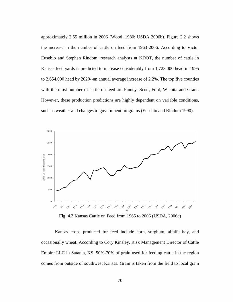
70
approximately 2.55 million in 2006 (Wood, 1980; USDA 2006b). Figure 2.2 shows
the increase in the number of cattle on feed from 1963-2006. According to Victor
Eusebio and Stephen Rindom, research analysts at KDOT, the number of cattle in
Kansas feed yards is predicted to increase considerably from 1,723,000 head in 1995
to 2,654,000 head by 2020--an annual average increase of 2.2%. The top five counties
with the most number of cattle on feed are Finney, Scott, Ford, Wichita and Grant.
However, these production predictions are highly dependent on variable conditions,
such as weather and changes to government programs (Eusebio and Rindom 1990).
Fig. 4.2 Kansas Cattle on Feed from 1965 to 2006 (USDA, 2006c)
Kansas crops produced for feed include corn, sorghum, alfalfa hay, and
occasionally wheat. According to Cory Kinsley, Risk Management Director of Cattle
Empire LLC in Satanta, KS, 50%-70% of grain used for feeding cattle in the region
comes from outside of southwest Kansas. Grain is taken from the field to local grain
0
500
1000
1500
2000
2500
3000
Cat
tle
On F
eed
(th
ou
sand
hea
d)
Year
71
elevators by trucks. An average Kansas elevator has a capacity of about 1.5 million
bushels. Grain elevators purchase the grain from farmers and then sell it to feed yards.
Feed yards will have the local grain picked up and brought to the feed yards by trucks
that generally only travel about 50 miles or less. Grain is also shipped to Kansas grain
elevators via rail shuttle trains from various locations in Iowa, Nebraska, and
Minnesota. At that point, the feed grains are trucked to the feed yards. According to
Charlie Sauerwein, Grain Merchant, and Kammi Schwarting, Financial Manager of
WindRiver Grain LLC in Garden City, Kansas, corn is shipped in from Iowa,
Minnesota, and Nebraska, and is then transported within Kansas. Corn is also moved
by trucks within a 30 mile radius to its destinations using independent freight
companies that operate on a contractual basis. Another type of feed is soybean meal,
which is shipped in from Emporia, Kansas and Nebraska. Local grain that is not used
in the area, mostly wheat, is shipped to other areas from local grain elevators by
shuttle train.
4.1.3 Meat Processing Industry
Meat processing companies purchase fattened cattle from various feed yards.
Each week, processing companies visit feed yards to survey cattle and make bids. The
cattle are sold on a live weight contract base and the processing companies arrange
the transportation since the packing manager needs to be in control of the efficiencies
of the plant. Once live cattle are slaughtered, their meat is processed and packaged for
shipment.

72
There are five major processing plants in Kansas with a combined daily kill
capacity of 27,600 (Bai et al. 2007). Four of the five major beef processing plants are
located in the southwest Kansas region and they have a combined daily kill capacity
of 23,600. These plants are National Beef in Dodge City and Liberal, KS; Excel
Corporation in Dodge City, KS; and Tyson Fresh Meats in Holcomb, KS. Even
though these plants have a combined daily kill capacity of 23,600, it is observed that
these plants do not run at full capacity the entire year because of market conditions.
These plants ship boxes of refrigerated beef all over the United States year round.

73
Chapter 5 Data Collection for Southwest Kansas Case Study
The estimation of highway damage costs associated with southwest Kansas
processed beef and related industries required several types of information. This
included truckload data on the highway section under study, truck characteristics,
pavement characteristics data, and pavement maintenance cost data. Truckload data
reflects the truck traffic on the highway section. Truck characteristics data are the
features of the trucks primarily used for the beef-related industry in southwest
Kansas. Required pavement characteristics data for this study included data
describing pavement type, length, structure, distress survey, and PSR performance.
This information was important for the pavement deterioration analysis. Pavement
maintenance cost data also needed to be collected to estimate average unit cost of the
highway section. The following sections describe the required data that were used for
this research in detail.
5.1 Truckload data
Modeling of traffic loadings is one important aspect in both pavement design
procedures but and in pavement deterioration models. To conduct this pavement
damage cost study, the first step was to estimate the annual truck VMTs attributed to
the processed beef and related industries on the highway pavement section under
study. This estimation required the annual truckload data on the studied highway
section. In the previous project by Bai et al. (2007), the truckloads generated by the
processed beef and related industries in the southeast Kansas area had been estimated,
74
including highway US 50/400 between Garden City and Dodge City. The truckload
data from a previous project was utilized for this research.
5.2 Truck Characteristics and type
The trucking industry has become a key player in the movement of freight in
the American economy because of its obvious advantages--promptness, constant
supervision, refrigeration, and effective tracking. Trucking has been the predominant
mode of freight transport for the processed meat industry in southwest Kansas (Bai et
al. 2007). Truck characteristics determine the way that the weight of trucks is actually
applied to highway pavements. Vehicle weight causes pavement damage as vehicles
travel along paved surfaces. Vehicle weight is frequently referred to as the gross
vehicle weight (GVW) or the total weight of the vehicle. GVW is the fixed weight of
the vehicle—such as the equipment, fuel, body, payload, and driver—on the basis of
an individual unit, such as a truck or tractor (Roadway Express 2005; General Motors
2006). However, GVW is not directly related to pavement deterioration. Axles
distribute the weight of a vehicle to a road surface, so pavement stress results from
the loads applied by axles or axle groups. In general, more axles result in less
pavement stress. Axle spacing also affects pavement loading. Axles placed close
together apply a load with less pavement stress (US DOT 2000). It is possible for a
vehicle with a greater GVW to result in less pavement damage than a lighter vehicle
due to the number and spacing of axles and axle groups.
75
5.2.1 Truck Axle Configurations
Basically there are five configurations for freight trucks (US DOT 2000):
Single-unit trucks
Truck-trailer combinations
Tractor-semitrailer combinations
Double-trailer combinations
Triple-trailer combinations
In general, a truck is a single unit vehicle that cannot be detached from its
freight bed and is composed of a single motorized device with more than two axles or
more than four tires (McCracken 2005). On the other hand, a tractor is a vehicle
designed preliminarily for pulling a trailer/semi-trailer that cannot be propelled on its
own. Various combinations of truck fleets can be seen in figure 5.1. Among the
various configurations, the tractor-semitrailer combinations account for more than
82% of all combinations of trucks on U.S. highways (US DOT 2000).
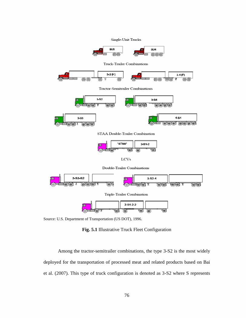
76
Source: U.S. Department of Transportation (US DOT), 1996.
Fig. 5.1 Illustrative Truck Fleet Configuration
Among the tractor-semitrailer combinations, the type 3-S2 is the most widely
deployed for the transportation of processed meat and related products based on Bai
et al. (2007). This type of truck configuration is denoted as 3-S2 where S represents
77
semitrailer and the number following S is the number of axles of the semitrailer (US
DOT 1996). The number preceding the ‗S‘ denotes the number of axles on the tractor.
The 3-S2 trucks were used for pavement damage assessment in this research.
In addition to axle configuration, pavement loadings are related to how weight
is distributed from a truck. Weight distribution involves how the cargo is actually
loaded onto the vehicle and how the vehicle is designed to carry its own components.
Criteria for the latter includes the engine, the cab, and the trailer. The loading
configuration indicates the amount of weight applied to each axle or axle group on a
fully loaded vehicle (Tolliver 1994). Trucks are designed for specific loading
configurations. Typically, loading configurations are described in the following
manner. Numbers are given which represent the weight applied to each axle group in
thousands of pounds. The numbers for specific axle groups are separated with
forward slash (/) symbols (Babcock et al. 2003).
5.2.2 Applying Truck Configuration in Pavement Deterioration Models
Modeling of traffic loadings on pavement is important in the pavement
deterioration models. Traffic loadings on pavement are directly related to weight
transferred to a road surface by vehicle axles. Axle load equivalency factors are used
to define the effects of different truck configurations. In addition to modeling the
effects of axle passes, it is necessary to measure the serviceability of pavement
segments for the estimation of pavement damage. The applications of truck and
pavement characteristics are key parts in this pavement damage cost study.
78
The effects of different truck axle configurations on pavements are estimated
by converting all axle loads to Equivalent Single Axle Loads (ESALs). An ESAL
refers to the equivalent effects of a single 18,000 pound axle load applied to a
pavement segment. An ESAL factor (n) is a standard reference load factor and
represents the equivalent pavement impact of an axle load as compared to a single
18,000-pound axle. For example, an axle with n = 1.2 has 1.2 times the impact of a
single 18,000-pound axle.
The steps in computing ESAL factors were: (1) computing the rate of
pavement deterioration for the reference axle, (2) computing the rate of pavement
deterioration for an axle load of interest, and (3) using the deterioration rates to
compute a load equivalency factor. The ESAL factor of an axle group depends upon
the type of axle (single, tandem, or triple), the load on the axle in thousands of pounds
(kips), the type of pavement section (flexible or rigid), and the terminal serviceability
rating of the pavement. The terminal serviceability rating is the value at which a
pavement is expected to be resurfaced or reconstructed.
5.3 Pavement Characteristics data
The pavement selected for this study is a section of highway US 50/400
between Dodge City and Garden City, Kansas. Figure 5.2 shows the location of the
highway section. This section of the highway was further divided into sub-sections or
segments. Pavement characteristics data were gathered for each segment, which
included functional class, pavement type, length, distress data, PSR, and structural
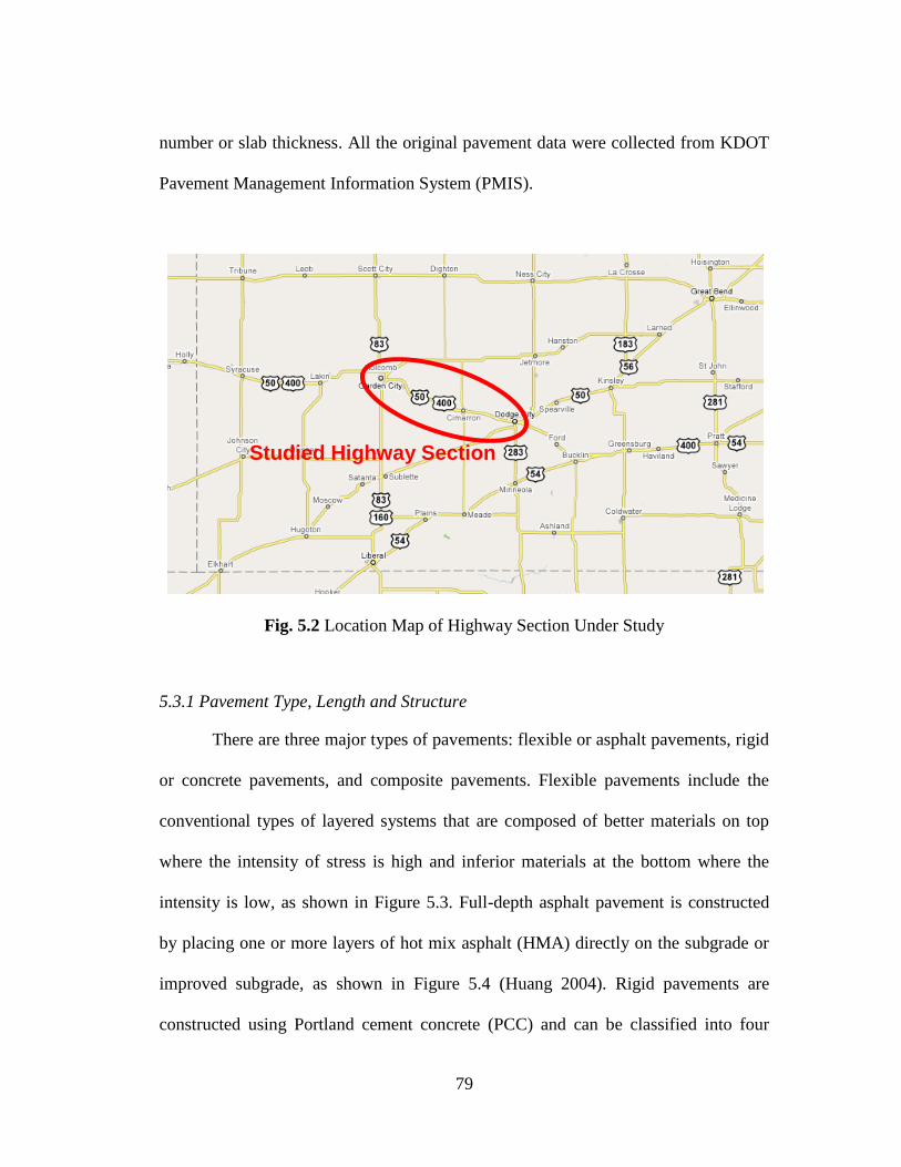
79
number or slab thickness. All the original pavement data were collected from KDOT
Pavement Management Information System (PMIS).
Fig. 5.2 Location Map of Highway Section Under Study
5.3.1 Pavement Type, Length and Structure
There are three major types of pavements: flexible or asphalt pavements, rigid
or concrete pavements, and composite pavements. Flexible pavements include the
conventional types of layered systems that are composed of better materials on top
where the intensity of stress is high and inferior materials at the bottom where the
intensity is low, as shown in Figure 5.3. Full-depth asphalt pavement is constructed
by placing one or more layers of hot mix asphalt (HMA) directly on the subgrade or
improved subgrade, as shown in Figure 5.4 (Huang 2004). Rigid pavements are
constructed using Portland cement concrete (PCC) and can be classified into four
Studied Highway Section
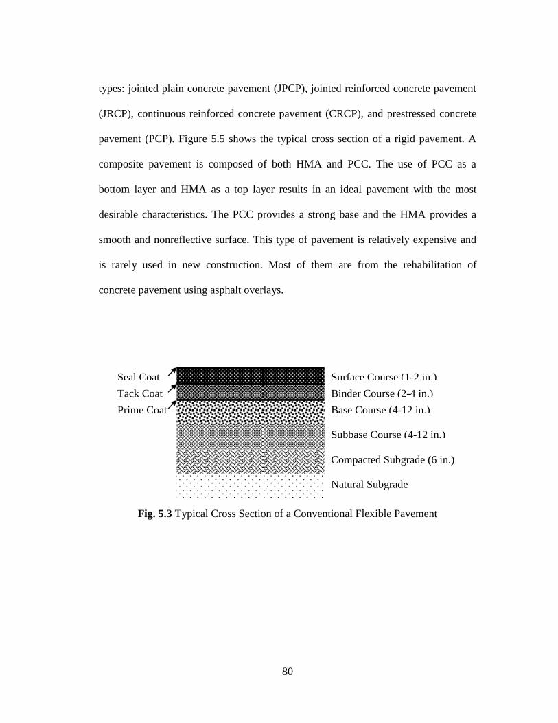
80
types: jointed plain concrete pavement (JPCP), jointed reinforced concrete pavement
(JRCP), continuous reinforced concrete pavement (CRCP), and prestressed concrete
pavement (PCP). Figure 5.5 shows the typical cross section of a rigid pavement. A
composite pavement is composed of both HMA and PCC. The use of PCC as a
bottom layer and HMA as a top layer results in an ideal pavement with the most
desirable characteristics. The PCC provides a strong base and the HMA provides a
smooth and nonreflective surface. This type of pavement is relatively expensive and
is rarely used in new construction. Most of them are from the rehabilitation of
concrete pavement using asphalt overlays.
Fig. 5.3 Typical Cross Section of a Conventional Flexible Pavement
Surface Course (1-2 in.)
Binder Course (2-4 in.)
Base Course (4-12 in.)
Subbase Course (4-12 in.)
Compacted Subgrade (6 in.)
Natural Subgrade
Seal Coat
Tack Coat
Prime Coat
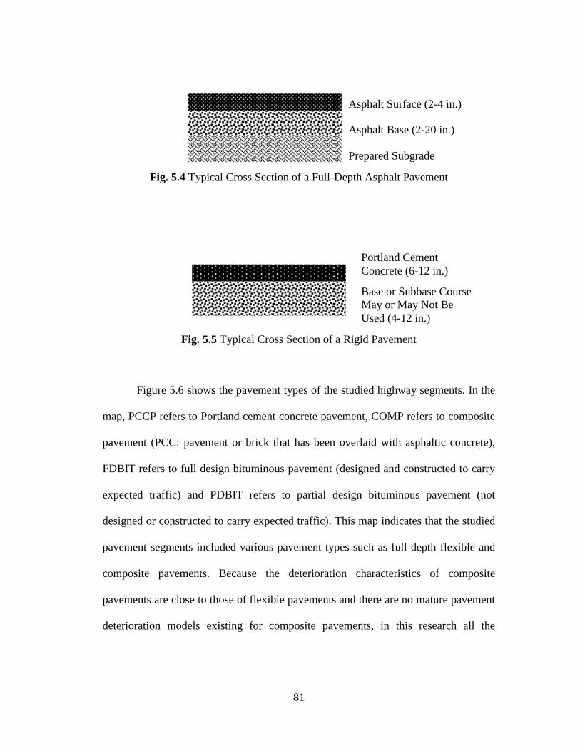
81
Fig. 5.4 Typical Cross Section of a Full-Depth Asphalt Pavement
Fig. 5.5 Typical Cross Section of a Rigid Pavement
Figure 5.6 shows the pavement types of the studied highway segments. In the
map, PCCP refers to Portland cement concrete pavement, COMP refers to composite
pavement (PCC: pavement or brick that has been overlaid with asphaltic concrete),
FDBIT refers to full design bituminous pavement (designed and constructed to carry
expected traffic) and PDBIT refers to partial design bituminous pavement (not
designed or constructed to carry expected traffic). This map indicates that the studied
pavement segments included various pavement types such as full depth flexible and
composite pavements. Because the deterioration characteristics of composite
pavements are close to those of flexible pavements and there are no mature pavement
deterioration models existing for composite pavements, in this research all the
Portland Cement
Concrete (6-12 in.)
Base or Subbase Course
May or May Not Be
Used (4-12 in.)
Asphalt Surface (2-4 in.)
Asphalt Base (2-20 in.)
Prepared Subgrade
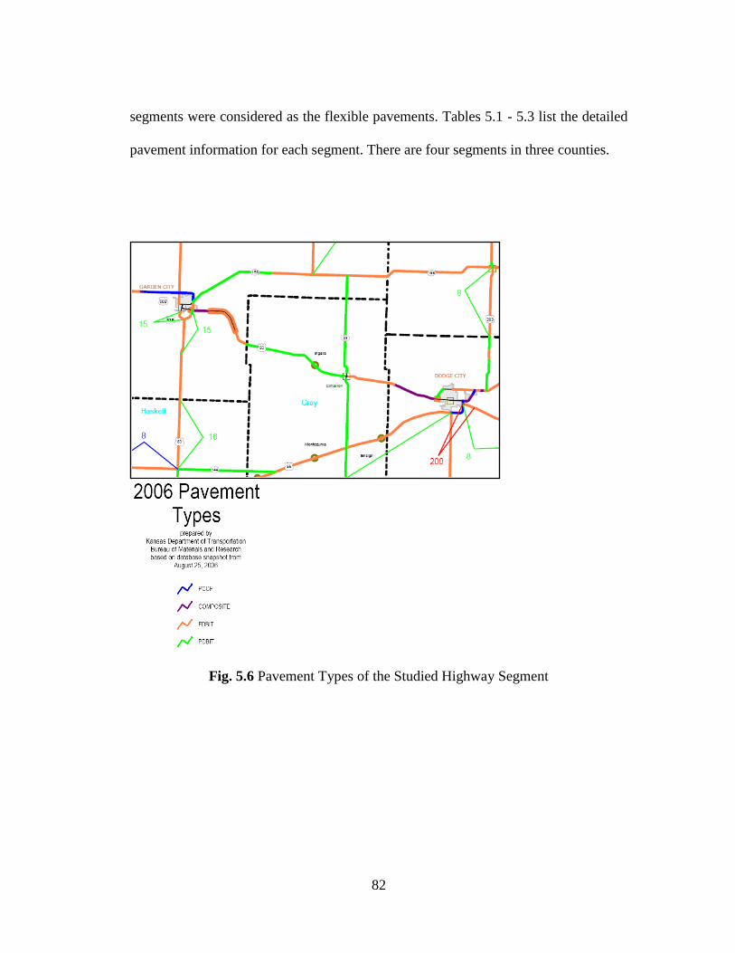
82
segments were considered as the flexible pavements. Tables 5.1 - 5.3 list the detailed
pavement information for each segment. There are four segments in three counties.
Fig. 5.6 Pavement Types of the Studied Highway Segment
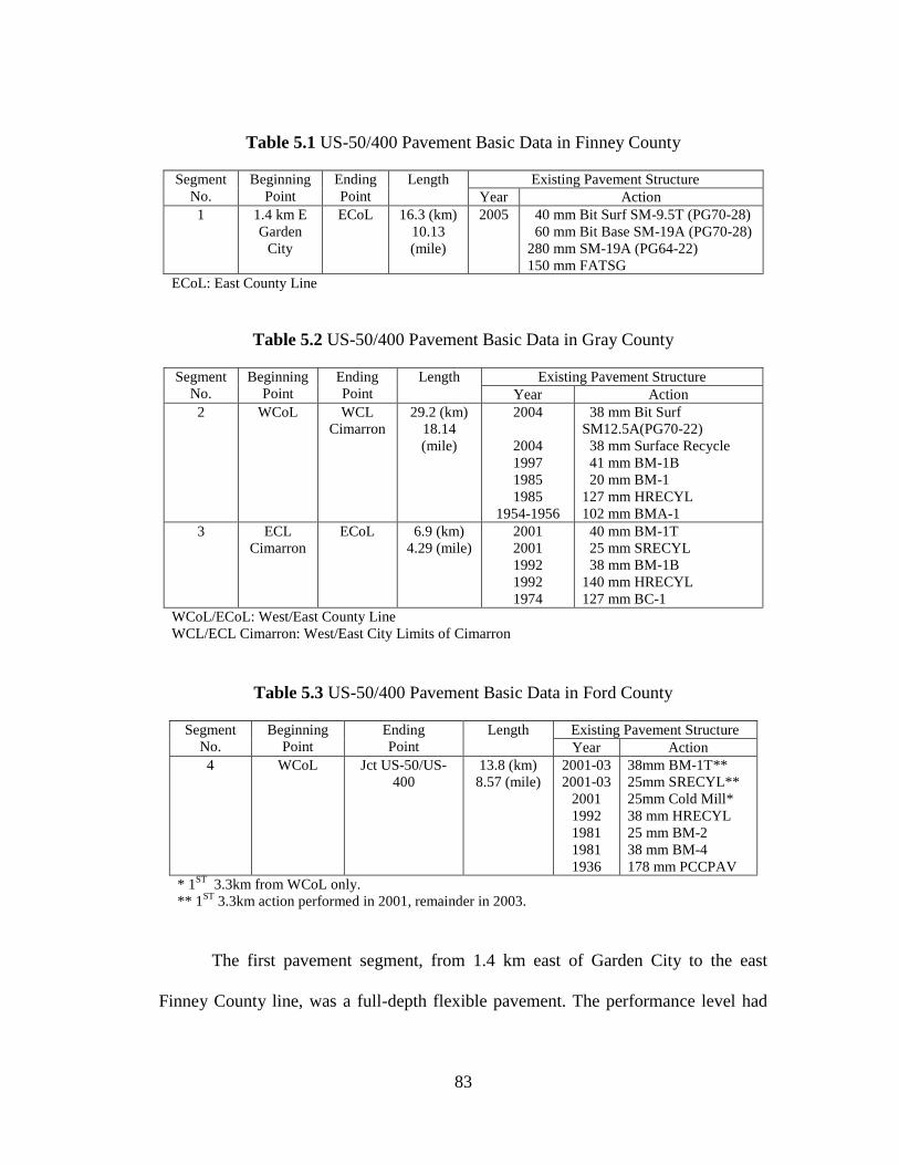
83
Table 5.1 US-50/400 Pavement Basic Data in Finney County
Segment
No.
Beginning
Point
Ending
Point
Length Existing Pavement Structure
Year Action
1 1.4 km E
Garden
City
ECoL
16.3 (km)
10.13
(mile)
2005 40 mm Bit Surf SM-9.5T (PG70-28)
60 mm Bit Base SM-19A (PG70-28)
280 mm SM-19A (PG64-22)
150 mm FATSG
ECoL: East County Line
Table 5.2 US-50/400 Pavement Basic Data in Gray County
Segment
No.
Beginning
Point
Ending
Point
Length
Existing Pavement Structure
Year Action
2 WCoL WCL
Cimarron
29.2 (km)
18.14
(mile)
2004
2004
1997
1985
1985
1954-1956
38 mm Bit Surf
SM12.5A(PG70-22)
38 mm Surface Recycle
41 mm BM-1B
20 mm BM-1
127 mm HRECYL
102 mm BMA-1
3 ECL
Cimarron
ECoL
6.9 (km)
4.29 (mile)
2001
2001
1992
1992
1974
40 mm BM-1T
25 mm SRECYL
38 mm BM-1B
140 mm HRECYL
127 mm BC-1
WCoL/ECoL: West/East County Line
WCL/ECL Cimarron: West/East City Limits of Cimarron
Table 5.3 US-50/400 Pavement Basic Data in Ford County
Segment
No.
Beginning
Point
Ending
Point
Length
Existing Pavement Structure
Year Action
4 WCoL
Jct US-50/US-
400
13.8 (km)
8.57 (mile)
2001-03
2001-03
2001
1992
1981
1981
1936
38mm BM-1T**
25mm SRECYL**
25mm Cold Mill*
38 mm HRECYL
25 mm BM-2
38 mm BM-4
178 mm PCCPAV
* 1ST
3.3km from WCoL only.
** 1ST
3.3km action performed in 2001, remainder in 2003.
The first pavement segment, from 1.4 km east of Garden City to the east
Finney County line, was a full-depth flexible pavement. The performance level had
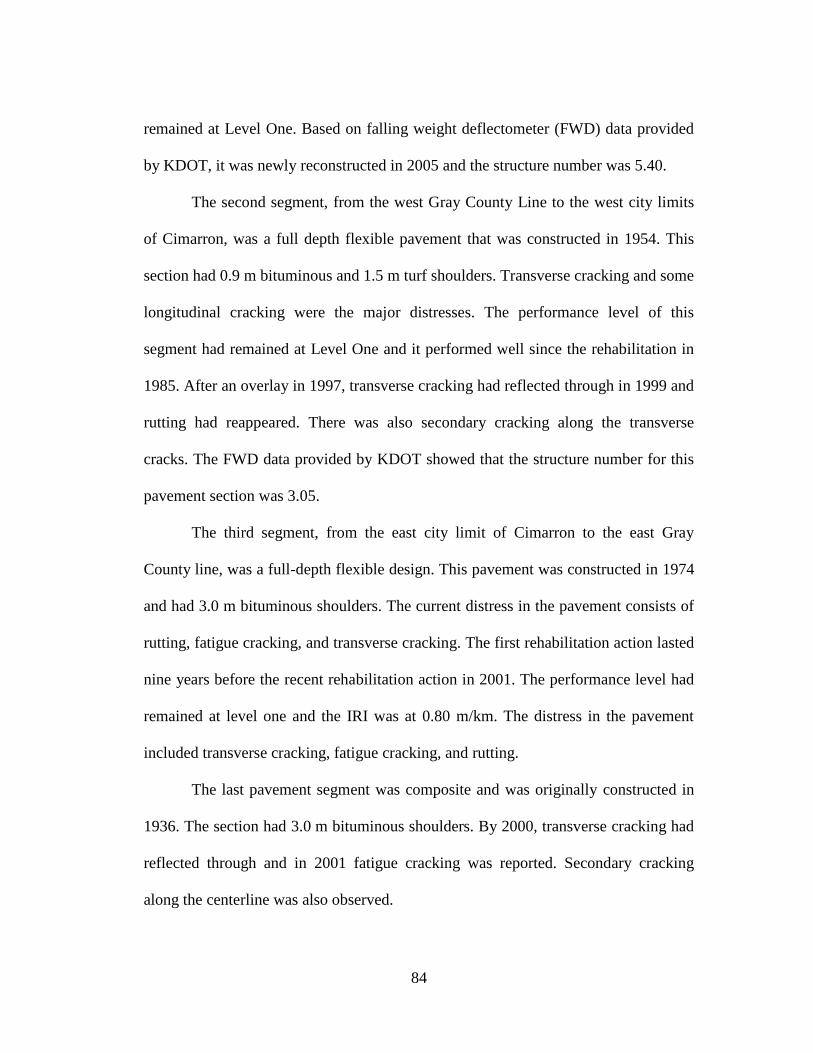
84
remained at Level One. Based on falling weight deflectometer (FWD) data provided
by KDOT, it was newly reconstructed in 2005 and the structure number was 5.40.
The second segment, from the west Gray County Line to the west city limits
of Cimarron, was a full depth flexible pavement that was constructed in 1954. This
section had 0.9 m bituminous and 1.5 m turf shoulders. Transverse cracking and some
longitudinal cracking were the major distresses. The performance level of this
segment had remained at Level One and it performed well since the rehabilitation in
1985. After an overlay in 1997, transverse cracking had reflected through in 1999 and
rutting had reappeared. There was also secondary cracking along the transverse
cracks. The FWD data provided by KDOT showed that the structure number for this
pavement section was 3.05.
The third segment, from the east city limit of Cimarron to the east Gray
County line, was a full-depth flexible design. This pavement was constructed in 1974
and had 3.0 m bituminous shoulders. The current distress in the pavement consists of
rutting, fatigue cracking, and transverse cracking. The first rehabilitation action lasted
nine years before the recent rehabilitation action in 2001. The performance level had
remained at level one and the IRI was at 0.80 m/km. The distress in the pavement
included transverse cracking, fatigue cracking, and rutting.
The last pavement segment was composite and was originally constructed in
1936. The section had 3.0 m bituminous shoulders. By 2000, transverse cracking had
reflected through and in 2001 fatigue cracking was reported. Secondary cracking
along the centerline was also observed.
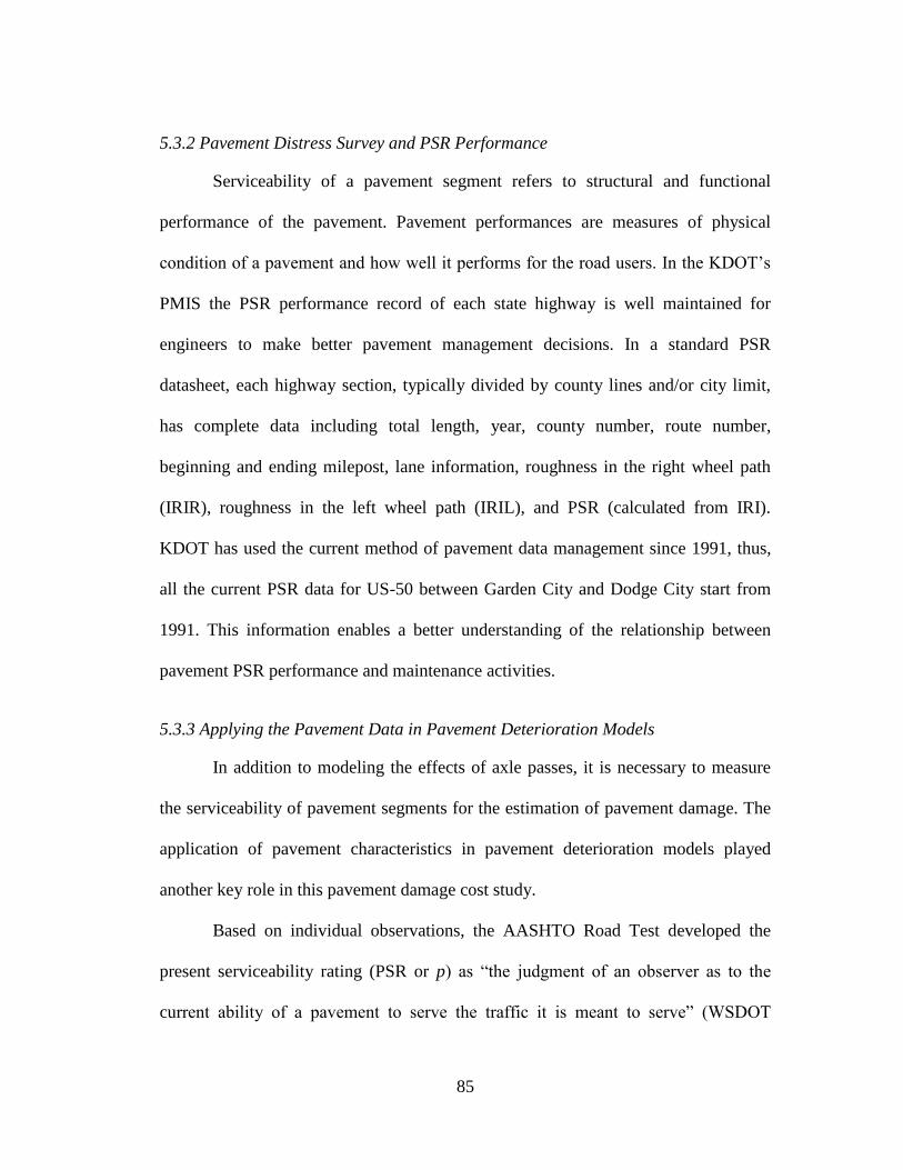
85
5.3.2 Pavement Distress Survey and PSR Performance
Serviceability of a pavement segment refers to structural and functional
performance of the pavement. Pavement performances are measures of physical
condition of a pavement and how well it performs for the road users. In the KDOT‘s
PMIS the PSR performance record of each state highway is well maintained for
engineers to make better pavement management decisions. In a standard PSR
datasheet, each highway section, typically divided by county lines and/or city limit,
has complete data including total length, year, county number, route number,
beginning and ending milepost, lane information, roughness in the right wheel path
(IRIR), roughness in the left wheel path (IRIL), and PSR (calculated from IRI).
KDOT has used the current method of pavement data management since 1991, thus,
all the current PSR data for US-50 between Garden City and Dodge City start from
1991. This information enables a better understanding of the relationship between
pavement PSR performance and maintenance activities.
5.3.3 Applying the Pavement Data in Pavement Deterioration Models
In addition to modeling the effects of axle passes, it is necessary to measure
the serviceability of pavement segments for the estimation of pavement damage. The
application of pavement characteristics in pavement deterioration models played
another key role in this pavement damage cost study.
Based on individual observations, the AASHTO Road Test developed the
present serviceability rating (PSR or p) as ―the judgment of an observer as to the
current ability of a pavement to serve the traffic it is meant to serve‖ (WSDOT
86
2003). The original AASHTO Road Test PSR scores were generated by observers
who drove along the test tracks and rated their ride quantitatively. This subjective
scale ranges from 5 (excellent) to 0 (very Poor). As Table 5.4 depicts, the PSR
considers the smoothness of the ride as well as the extent of rutting and other
distresses. Modeling a decline in PSR is, to a certain extent, modeling the occurrence
of individual distresses as well.
In the state of Kansas KDOT designs for an initial PSR of 4.2 and a terminal
PSR of 2.5. Subtracting the terminal PSR from the initial PSR gives the maximum
life of a truck route pavement in terms of tolerable decline in PSR. This value is 1.7
for Kansas state highways.
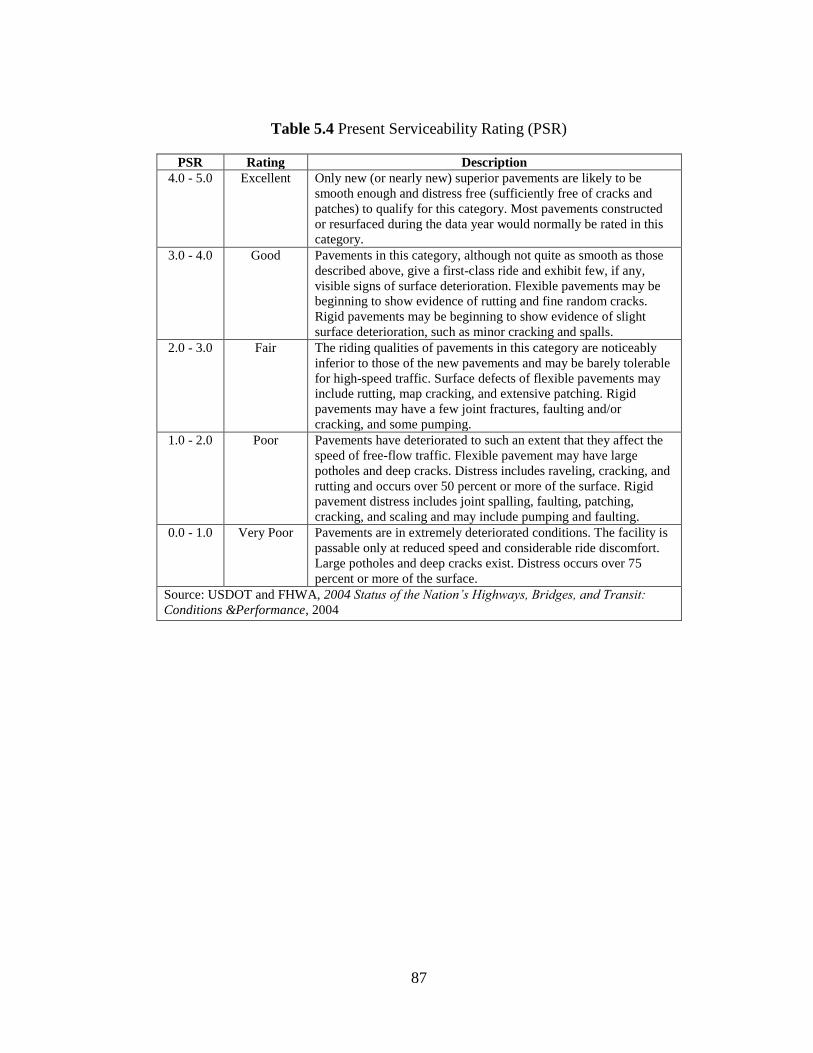
87
Table 5.4 Present Serviceability Rating (PSR)
PSR Rating Description
4.0 - 5.0 Excellent Only new (or nearly new) superior pavements are likely to be
smooth enough and distress free (sufficiently free of cracks and
patches) to qualify for this category. Most pavements constructed
or resurfaced during the data year would normally be rated in this
category.
3.0 - 4.0 Good Pavements in this category, although not quite as smooth as those
described above, give a first-class ride and exhibit few, if any,
visible signs of surface deterioration. Flexible pavements may be
beginning to show evidence of rutting and fine random cracks.
Rigid pavements may be beginning to show evidence of slight
surface deterioration, such as minor cracking and spalls.
2.0 - 3.0 Fair The riding qualities of pavements in this category are noticeably
inferior to those of the new pavements and may be barely tolerable
for high-speed traffic. Surface defects of flexible pavements may
include rutting, map cracking, and extensive patching. Rigid
pavements may have a few joint fractures, faulting and/or
cracking, and some pumping.
1.0 - 2.0 Poor Pavements have deteriorated to such an extent that they affect the
speed of free-flow traffic. Flexible pavement may have large
potholes and deep cracks. Distress includes raveling, cracking, and
rutting and occurs over 50 percent or more of the surface. Rigid
pavement distress includes joint spalling, faulting, patching,
cracking, and scaling and may include pumping and faulting.
0.0 - 1.0 Very Poor Pavements are in extremely deteriorated conditions. The facility is
passable only at reduced speed and considerable ride discomfort.
Large potholes and deep cracks exist. Distress occurs over 75
percent or more of the surface.
Source: USDOT and FHWA, 2004 Status of the Nation’s Highways, Bridges, and Transit:
Conditions &Performance, 2004
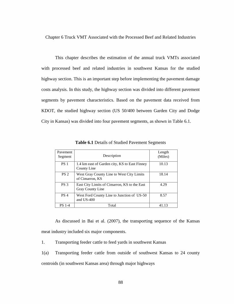
88
Chapter 6 Truck VMT Associated with the Processed Beef and Related Industries
This chapter describes the estimation of the annual truck VMTs associated
with processed beef and related industries in southwest Kansas for the studied
highway section. This is an important step before implementing the pavement damage
costs analysis. In this study, the highway section was divided into different pavement
segments by pavement characteristics. Based on the pavement data received from
KDOT, the studied highway section (US 50/400 between Garden City and Dodge
City in Kansas) was divided into four pavement segments, as shown in Table 6.1.
Table 6.1 Details of Studied Pavement Segments
Pavement
Segment Description Length
(Miles)
PS 1 1.4 km east of Garden city, KS to East Finney
County Line
10.13
PS 2 West Gray County Line to West City Limits
of Cimarron, KS
18.14
PS 3 East City Limits of Cimarron, KS to the East
Gray County Line
4.29
PS 4 West Ford County Line to Junction of US-50
and US-400
8.57
PS 1-4 Total 41.13
As discussed in Bai et al. (2007), the transporting sequence of the Kansas
meat industry included six major components.
1. Transporting feeder cattle to feed yards in southwest Kansas
1(a) Transporting feeder cattle from outside of southwest Kansas to 24 county
centroids (in southwest Kansas area) through major highways
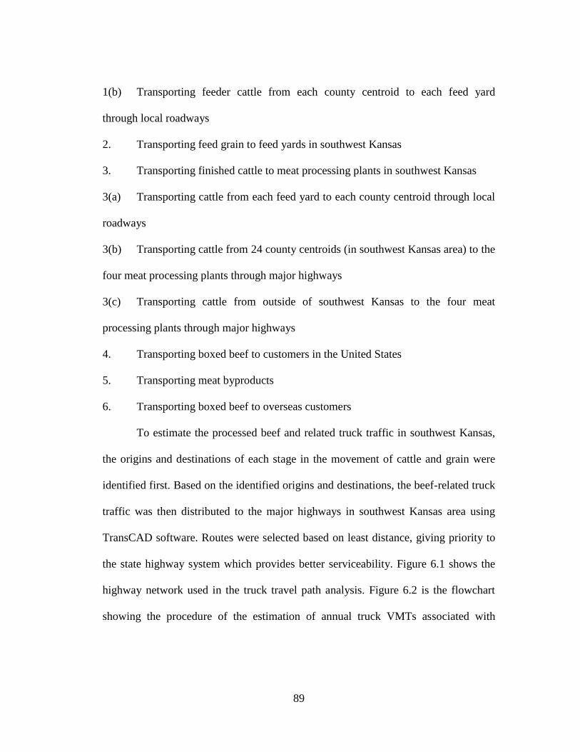
89
1(b) Transporting feeder cattle from each county centroid to each feed yard
through local roadways
2. Transporting feed grain to feed yards in southwest Kansas
3. Transporting finished cattle to meat processing plants in southwest Kansas
3(a) Transporting cattle from each feed yard to each county centroid through local
roadways
3(b) Transporting cattle from 24 county centroids (in southwest Kansas area) to the
four meat processing plants through major highways
3(c) Transporting cattle from outside of southwest Kansas to the four meat
processing plants through major highways
4. Transporting boxed beef to customers in the United States
5. Transporting meat byproducts
6. Transporting boxed beef to overseas customers
To estimate the processed beef and related truck traffic in southwest Kansas,
the origins and destinations of each stage in the movement of cattle and grain were
identified first. Based on the identified origins and destinations, the beef-related truck
traffic was then distributed to the major highways in southwest Kansas area using
TransCAD software. Routes were selected based on least distance, giving priority to
the state highway system which provides better serviceability. Figure 6.1 shows the
highway network used in the truck travel path analysis. Figure 6.2 is the flowchart
showing the procedure of the estimation of annual truck VMTs associated with

90
processed beef and related industries. Detailed descriptions are provided in the
following sections.
91
Fig
. 6.1
South
wes
t K
ansa
s H
ighw
ay M
ap (
Sourc
e: K
DO
T 2
005)
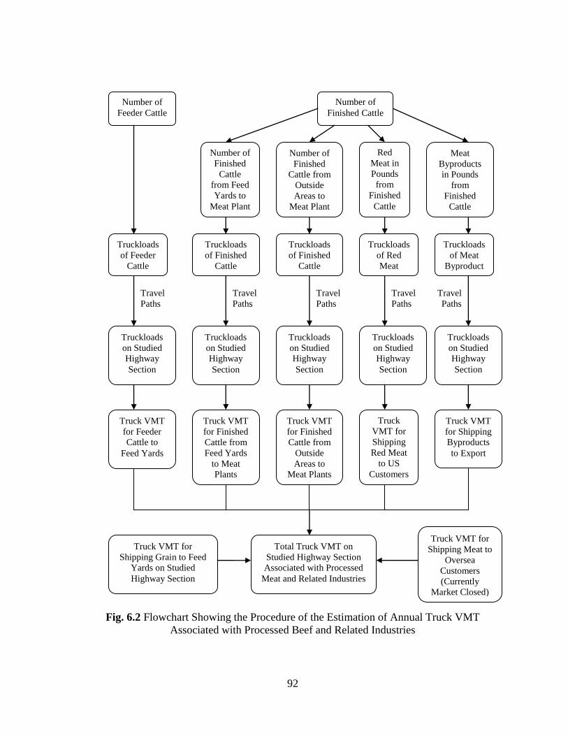
92
Fig. 6.2 Flowchart Showing the Procedure of the Estimation of Annual Truck VMT
Associated with Processed Beef and Related Industries
Travel
Paths
Travel
Paths
Travel
Paths
Travel
Paths
Travel
Paths
Number of
Feeder Cattle
Truckloads
of Feeder
Cattle
Truckloads
on Studied
Highway
Section
Truck VMT
for Feeder
Cattle to
Feed Yards
Number of
Finished Cattle
Number of
Finished
Cattle
from Feed
Yards to
Meat Plant
Red
Meat in
Pounds
from
Finished
Cattle
Meat
Byproducts
in Pounds
from
Finished
Cattle
Number of
Finished
Cattle from
Outside
Areas to
Meat Plant
Truckloads
of Finished
Cattle
Truckloads
of Finished
Cattle
Truckloads
of Red
Meat
Truckloads
of Meat
Byproduct
s
Truckloads
on Studied
Highway
Section
Truckloads
on Studied
Highway
Section
Truckloads
on Studied
Highway
Section
Truckloads
on Studied
Highway
Section
Truck VMT
for Finished
Cattle from
Feed Yards
to Meat
Plants
Truck VMT
for Finished
Cattle from
Outside
Areas to
Meat Plants
Truck
VMT for
Shipping
Red Meat
to US
Customers
Truck VMT
for Shipping
Byproducts
to Export
Total Truck VMT on
Studied Highway Section
Associated with Processed
Meat and Related Industries
Truck VMT for
Shipping Grain to Feed
Yards on Studied
Highway Section
Truck VMT for
Shipping Meat to
Oversea
Customers
(Currently
Market Closed)
93
6.1 Truck VMT for Transporting Feeder Cattle to Feed Yards
6.1.1 Truck Travel Paths for Transporting Feeder Cattle to Feed Yards
The cattle in southwest Kansas were assumed to be transported to the region
for feeding from other states and/or other parts of Kansas. As shown in Figure 1.2,
there were approximately 369 feed yards located within the 24 counties of the
southwest Kansas region. Figure 6.3 shows the 24 counties of the analysis area with
its centroid and the major highways. For this analysis, a centroid was defined as the
aggregation of the feed yards within a county. Additionally, a centroid for each
county must be located on a highway. The truck travel paths for transporting feeder
cattle to feed yards were estimated based on two steps: (1) from entry points of the
southwest Kansas boundary to county centroids, and (2) from the centroid of a county
to the feed yards within this same county in the study area.
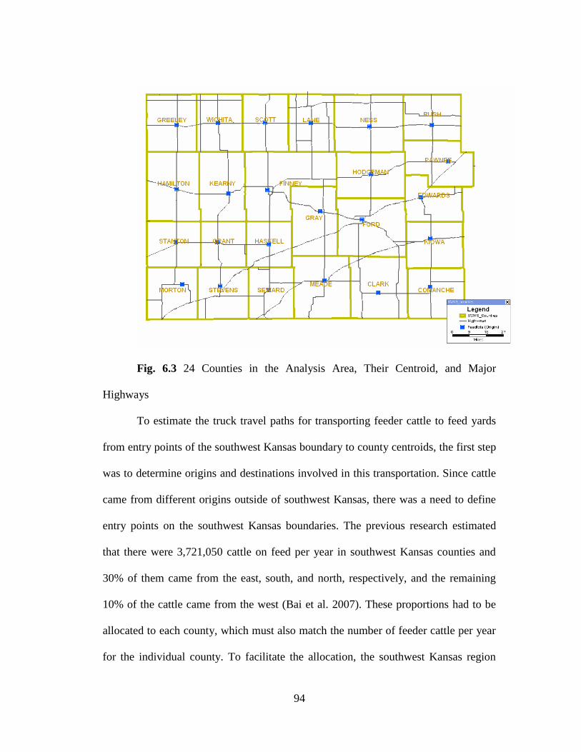
94
Fig. 6.3 24 Counties in the Analysis Area, Their Centroid, and Major
Highways
To estimate the truck travel paths for transporting feeder cattle to feed yards
from entry points of the southwest Kansas boundary to county centroids, the first step
was to determine origins and destinations involved in this transportation. Since cattle
came from different origins outside of southwest Kansas, there was a need to define
entry points on the southwest Kansas boundaries. The previous research estimated
that there were 3,721,050 cattle on feed per year in southwest Kansas counties and
30% of them came from the east, south, and north, respectively, and the remaining
10% of the cattle came from the west (Bai et al. 2007). These proportions had to be
allocated to each county, which must also match the number of feeder cattle per year
for the individual county. To facilitate the allocation, the southwest Kansas region
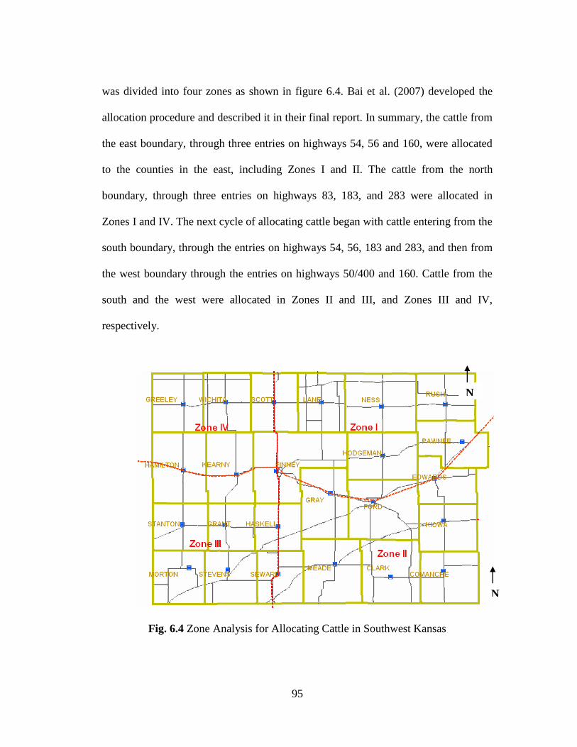
95
was divided into four zones as shown in figure 6.4. Bai et al. (2007) developed the
allocation procedure and described it in their final report. In summary, the cattle from
the east boundary, through three entries on highways 54, 56 and 160, were allocated
to the counties in the east, including Zones I and II. The cattle from the north
boundary, through three entries on highways 83, 183, and 283 were allocated in
Zones I and IV. The next cycle of allocating cattle began with cattle entering from the
south boundary, through the entries on highways 54, 56, 183 and 283, and then from
the west boundary through the entries on highways 50/400 and 160. Cattle from the
south and the west were allocated in Zones II and III, and Zones III and IV,
respectively.
Fig. 6.4 Zone Analysis for Allocating Cattle in Southwest Kansas
N
N
96
Table 6.2 summarizes the feeder cattle allocation sequence and the highway
entrances. In the Highway Entry Point column of the table the first letter of each entry
point highway represents the direction, and the following number represents the
highway number. For instance, E54 represents highway 54 in the east boundary of
southwest Kansas.
Appendix I lists the shortest-path analysis results for transporting feeder cattle
from a county centroid to feed yards in each of the studied counties. Results showed
that all the travel paths were on local roads and thus they were not considered in this
study.
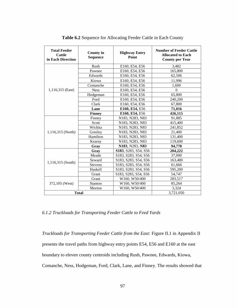
97
Table 6.2 Sequence for Allocating Feeder Cattle in Each County
Total Feeder
Cattle
in Each Direction
County in
Sequence
Highway Entry
Point
Number of Feeder Cattle
Allocated to Each
County per Year
1,116,315 (East)
Rush E160, E54, E56 3,482
Pawnee E160, E54, E56 165,800
Edwards E160, E54, E56 62,506
Kiowa E160, E54, E56 11,996
Comanche E160, E54, E56 1,600
Ness E160, E54, E56 0
Hodgeman E160, E54, E56 65,800
Ford E160, E54, E56 240,200
Clark E160, E54, E56 67,800
Lane E160, E54, E56 71,016
Finney E160, E54, E56 426,115
1,116,315 (North)
Finney N183, N283, N83 91,885
Scott N183, N283, N83 415,400
Wichita N183, N283, N83 241,852
Greeley N183, N283, N83 21,400
Hamilton N183, N283, N83 131,400
Kearny N183, N283, N83 119,600
Gray N183, N283, N83 94,778
1,116,315 (South)
Gray S183, S283, S54, S56 204,222
Meade S183, S283, S54, S56 37,000
Seward S183, S283, S54, S56 163,480
Stevens S183, S283, S54, S56 61,666
Haskell S183, S283, S54, S56 595,200
Grant S183, S283, S54, S56 54,747
372,105 (West)
Grant W160, W50/400 283,517
Stanton W160, W50/400 85,264
Morton W160, W50/400 3,324
Total 3,721,050
6.1.2 Truckloads for Transporting Feeder Cattle to Feed Yards
Truckloads for Transporting Feeder Cattle from the East: Figure II.1 in Appendix II
presents the travel paths from highway entry points E54, E56 and E160 at the east
boundary to eleven county centroids including Rush, Pawnee, Edwards, Kiowa,
Comanche, Ness, Hodgeman, Ford, Clark, Lane, and Finney. The results showed that
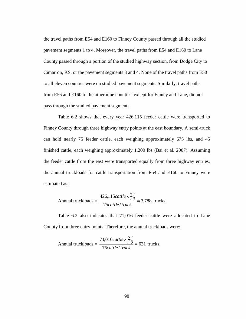
98
the travel paths from E54 and E160 to Finney County passed through all the studied
pavement segments 1 to 4. Moreover, the travel paths from E54 and E160 to Lane
County passed through a portion of the studied highway section, from Dodge City to
Cimarron, KS, or the pavement segments 3 and 4. None of the travel paths from E50
to all eleven counties were on studied pavement segments. Similarly, travel paths
from E56 and E160 to the other nine counties, except for Finney and Lane, did not
pass through the studied pavement segments.
Table 6.2 shows that every year 426,115 feeder cattle were transported to
Finney County through three highway entry points at the east boundary. A semi-truck
can hold nearly 75 feeder cattle, each weighing approximately 675 lbs, and 45
finished cattle, each weighing approximately 1,200 lbs (Bai et al. 2007). Assuming
the feeder cattle from the east were transported equally from three highway entries,
the annual truckloads for cattle transportation from E54 and E160 to Finney were
estimated as:
Annual truckloads = 788,3/75
32115,426
truckcattle
cattle trucks.
Table 6.2 also indicates that 71,016 feeder cattle were allocated to Lane
County from three entry points. Therefore, the annual truckloads were:
Annual truckloads = 631/75
32016,71
truckcattle
cattle trucks.
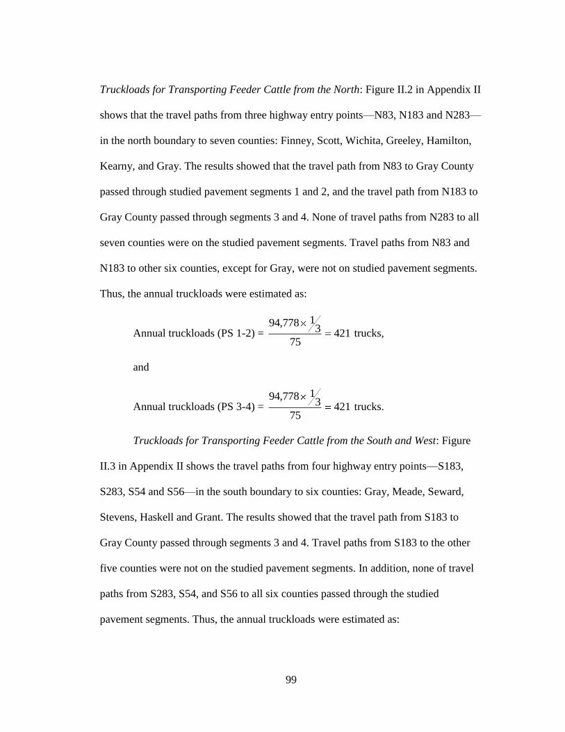
99
Truckloads for Transporting Feeder Cattle from the North: Figure II.2 in Appendix II
shows that the travel paths from three highway entry points—N83, N183 and N283—
in the north boundary to seven counties: Finney, Scott, Wichita, Greeley, Hamilton,
Kearny, and Gray. The results showed that the travel path from N83 to Gray County
passed through studied pavement segments 1 and 2, and the travel path from N183 to
Gray County passed through segments 3 and 4. None of travel paths from N283 to all
seven counties were on the studied pavement segments. Travel paths from N83 and
N183 to other six counties, except for Gray, were not on studied pavement segments.
Thus, the annual truckloads were estimated as:
Annual truckloads (PS 1-2) = 42175
31778,94
trucks,
and
Annual truckloads (PS 3-4) = 42175
31778,94
trucks.
Truckloads for Transporting Feeder Cattle from the South and West: Figure
II.3 in Appendix II shows the travel paths from four highway entry points—S183,
S283, S54 and S56—in the south boundary to six counties: Gray, Meade, Seward,
Stevens, Haskell and Grant. The results showed that the travel path from S183 to
Gray County passed through segments 3 and 4. Travel paths from S183 to the other
five counties were not on the studied pavement segments. In addition, none of travel
paths from S283, S54, and S56 to all six counties passed through the studied
pavement segments. Thus, the annual truckloads were estimated as:
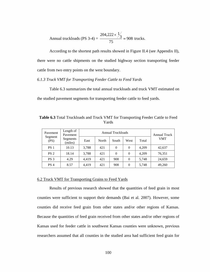
100
Annual truckloads (PS 3-4) = 90875
31222,204
trucks.
According to the shortest path results showed in Figure II.4 (see Appendix II),
there were no cattle shipments on the studied highway section transporting feeder
cattle from two entry points on the west boundary.
6.1.3 Truck VMT for Transporting Feeder Cattle to Feed Yards
Table 6.3 summarizes the total annual truckloads and truck VMT estimated on
the studied pavement segments for transporting feeder cattle to feed yards.
Table 6.3 Total Truckloads and Truck VMT for Transporting Feeder Cattle to Feed
Yards
Pavement
Segment
(PS)
Length of
Pavement
Segments
(miles)
Annual Truckloads Annual Truck
VMT East North South West Total
PS 1 10.13 3,788 421 0 0 4,209 42,637
PS 2 18.14 3,788 421 0 0 4,209 76,351
PS 3 4.29 4,419 421 908 0 5,748 24,659
PS 4 8.57 4,419 421 908 0 5,748 49,260
6.2 Truck VMT for Transporting Grains to Feed Yards
Results of previous research showed that the quantities of feed grain in most
counties were sufficient to support their demands (Bai et al. 2007). However, some
counties did receive feed grain from other states and/or other regions of Kansas.
Because the quantities of feed grain received from other states and/or other regions of
Kansas used for feeder cattle in southwest Kansas counties were unknown, previous
researchers assumed that all counties in the studied area had sufficient feed grain for
101
their feed yards. With this assumption, the county centroids in this analysis were also
defined as grain elevator stations that distributed the feed grain to each feed yard in
the respective county.
Appendix I shows the shortest path results for transporting grain from a
county centroid to feed yards in each respective county and these paths are the same
as those for transporting feeder cattle. None of the paths used by feed grain
transportation were on major highways. Therefore, no truck VMTs associated with
the grain transportation were considered for the pavement damage analysis.
6.3 Truck VMT for Transporting Finished Cattle to Meat Processing Plants
Based on USDA data, there were 7,321,400 cattle slaughtered in Kansas in
2005. According to the data collected from the four largest meat processing facilities
in the southwest Kansas region, approximately 23,600 cattle were slaughtered every
day. In addition, about 4,000 cattle per day were slaughtered in another large meat
processing facility in Kansas, but it was not in the southwest Kansas region. Thus,
approximately, a total of 27,600 cattle were killed daily in Kansas. The number of
cattle slaughtered in the southwest Kansas region in 2005 was estimated
proportionally as follows (Bai et al. 2007):
Number of cattle slaughtered = 7,321,400 x (23,600 / 27,600) = 6,260,330.
In 2005, there were 3,721,050 cattle fed in southwest Kansas area. If it is
assumed that all cattle fed in southwest Kansas were slaughtered in the southwest
Kansas, then 2,539,280 (6,260,330 – 3,721,050) additional cattle would have to have
been transported into southwest Kansas from other states and/or other parts of Kansas
102
(Bai et al. 2007). The cattle from both inside and outside of southwest Kansas were
then delivered to the four major meat processing plants. These plants include the
Excel Corporation in Dodge City, National Beef in Dodge City, National Beef in
Liberty, and Tyson Fresh Meats in Holcomb. Two steps were involved in the
calculation of the truck VMT for transporting cattle to four meat processing facilities
in southwest Kansas. (1) Estimating the truck VMT generated by transporting cattle
from feed yards in southwest Kansas to the meat processing facilities, which included
transporting cattle from feed yards to county centroids and then transporting from this
location to the four meat plants. (2) Estimating the truck VMT for transporting cattle
from other states and/or other parts of Kansas to meat processing facilities in
southwest Kansas.
6.3.1 Truck VMT for Transporting Cattle from Feed Yards in Southwest Kansas to
Meat Processing Plants
Appendix I shows the same shortest paths for transporting finished cattle from
feed yards to county centroids as those for transporting feeder cattle from county
centroids to feed yards with reversed origins and destinations. Since those local travel
paths had no impact on the highway section used for this pavement damage analysis,
they are not discussed further.
After the finished cattle were transported to the county centroids they were
then shipped to the four major meat processing facilities in the southwest Kansas
region for slaughter. To simplify the distribution process, it was assumed that an
average of 25% of the annual truckloads from each county was distributed to each of
103
the four major meat processing facilities. Thus, the annual truckloads from each of
the county centroids to each of the four meat processing facilities in the southwest
Kansas region were calculated using the following formula.
Annual truckloads from a county centroid to a meat processing facility
= 25% x annual truckloads of a county.
In addition to the annual truckloads from each county centroid to the four
meat processing facilities, there was a need to find out the truck travel paths from
each county centroid to each of the four meat processing facilities. This was
necessary in order to estimate the VMT on the studied highway pavement segments.
These paths were determined using TransCAD software based on the shortest path
method and the results are shown in Appendix III. In the TransCAD analyses the
origins were twenty-four county centroids and the destinations were four meat
processing plants.
Annual truckloads for transporting finished cattle from each county to each
meat processing plant were determined in previous research and results were shown
in Table 6.4 to 6.7. Based on truck travel paths shown in figures of Appendix III,
Table 6.8 was developed to summarize the truckloads and identify the impacted
pavement segments. Note that none of the trucks transporting cattle to the National
Beef Liberal plant utilized the studied highway section, thus, this plant was not
included in Table 6.8.
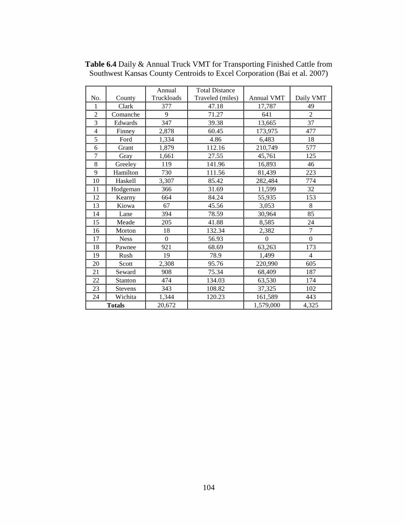
104
Table 6.4 Daily & Annual Truck VMT for Transporting Finished Cattle from
Southwest Kansas County Centroids to Excel Corporation (Bai et al. 2007)
No. County
Annual
Truckloads
Total Distance
Traveled (miles) Annual VMT Daily VMT
1 Clark 377 47.18 17,787 49
2 Comanche 9 71.27 641 2
3 Edwards 347 39.38 13,665 37
4 Finney 2,878 60.45 173,975 477
5 Ford 1,334 4.86 6,483 18
6 Grant 1,879 112.16 210,749 577
7 Gray 1,661 27.55 45,761 125
8 Greeley 119 141.96 16,893 46
9 Hamilton 730 111.56 81,439 223
10 Haskell 3,307 85.42 282,484 774
11 Hodgeman 366 31.69 11,599 32
12 Kearny 664 84.24 55,935 153
13 Kiowa 67 45.56 3,053 8
14 Lane 394 78.59 30,964 85
15 Meade 205 41.88 8,585 24
16 Morton 18 132.34 2,382 7
17 Ness 0 56.93 0 0
18 Pawnee 921 68.69 63,263 173
19 Rush 19 78.9 1,499 4
20 Scott 2,308 95.76 220,990 605
21 Seward 908 75.34 68,409 187
22 Stanton 474 134.03 63,530 174
23 Stevens 343 108.82 37,325 102
24 Wichita 1,344 120.23 161,589 443
Totals 20,672 1,579,000 4,325
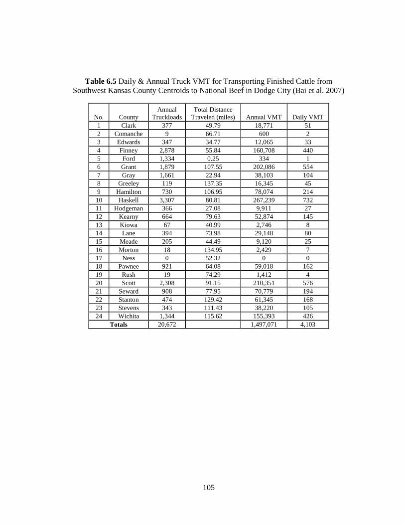
105
Table 6.5 Daily & Annual Truck VMT for Transporting Finished Cattle from
Southwest Kansas County Centroids to National Beef in Dodge City (Bai et al. 2007)
No. County
Annual
Truckloads
Total Distance
Traveled (miles) Annual VMT Daily VMT
1 Clark 377 49.79 18,771 51
2 Comanche 9 66.71 600 2
3 Edwards 347 34.77 12,065 33
4 Finney 2,878 55.84 160,708 440
5 Ford 1,334 0.25 334 1
6 Grant 1,879 107.55 202,086 554
7 Gray 1,661 22.94 38,103 104
8 Greeley 119 137.35 16,345 45
9 Hamilton 730 106.95 78,074 214
10 Haskell 3,307 80.81 267,239 732
11 Hodgeman 366 27.08 9,911 27
12 Kearny 664 79.63 52,874 145
13 Kiowa 67 40.99 2,746 8
14 Lane 394 73.98 29,148 80
15 Meade 205 44.49 9,120 25
16 Morton 18 134.95 2,429 7
17 Ness 0 52.32 0 0
18 Pawnee 921 64.08 59,018 162
19 Rush 19 74.29 1,412 4
20 Scott 2,308 91.15 210,351 576
21 Seward 908 77.95 70,779 194
22 Stanton 474 129.42 61,345 168
23 Stevens 343 111.43 38,220 105
24 Wichita 1,344 115.62 155,393 426
Totals 20,672 1,497,071 4,103
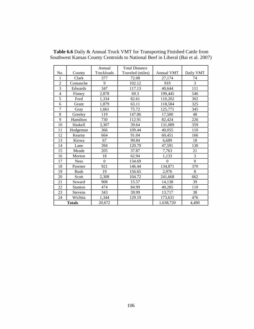
106
Table 6.6 Daily & Annual Truck VMT for Transporting Finished Cattle from
Southwest Kansas County Centroids to National Beef in Liberal (Bai et al. 2007)
No. County
Annual
Truckloads
Total Distance
Traveled (miles) Annual VMT Daily VMT
1 Clark 377 72.08 27,174 74
2 Comanche 9 102.12 919 3
3 Edwards 347 117.13 40,644 111
4 Finney 2,878 69.3 199,445 546
5 Ford 1,334 82.61 110,202 302
6 Grant 1,879 63.11 118,584 325
7 Gray 1,661 75.72 125,771 345
8 Greeley 119 147.06 17,500 48
9 Hamilton 730 112.91 82,424 226
10 Haskell 3,307 39.64 131,089 359
11 Hodgeman 366 109.44 40,055 110
12 Kearny 664 91.04 60,451 166
13 Kiowa 67 99.84 6,689 18
14 Lane 394 120.79 47,591 130
15 Meade 205 37.87 7,763 21
16 Morton 18 62.94 1,133 3
17 Ness 0 134.69 0 0
18 Pawnee 921 146.44 134,871 370
19 Rush 19 156.65 2,976 8
20 Scott 2,308 104.72 241,668 662
21 Seward 908 15.57 14,138 39
22 Stanton 474 84.99 40,285 110
23 Stevens 343 39.99 13,717 38
24 Wichita 1,344 129.19 173,631 476
Totals 20,672 1,638,720 4,490
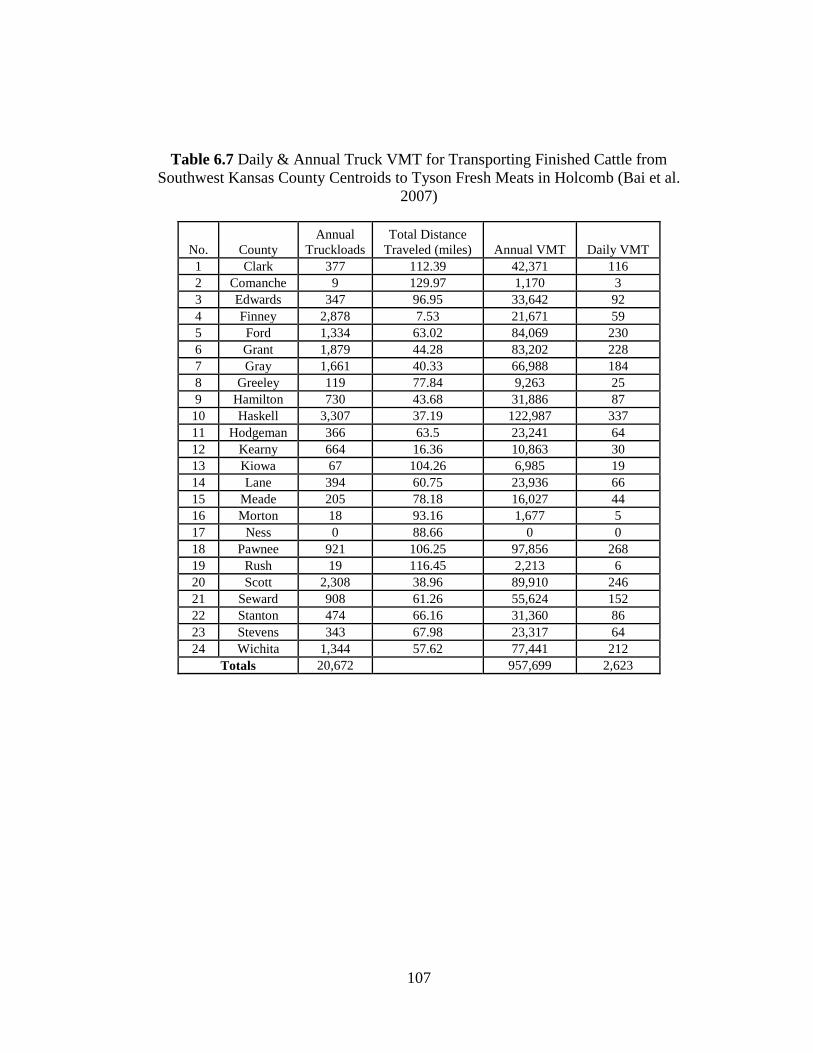
107
Table 6.7 Daily & Annual Truck VMT for Transporting Finished Cattle from
Southwest Kansas County Centroids to Tyson Fresh Meats in Holcomb (Bai et al.
2007)
No. County
Annual
Truckloads
Total Distance
Traveled (miles) Annual VMT Daily VMT
1 Clark 377 112.39 42,371 116
2 Comanche 9 129.97 1,170 3
3 Edwards 347 96.95 33,642 92
4 Finney 2,878 7.53 21,671 59
5 Ford 1,334 63.02 84,069 230
6 Grant 1,879 44.28 83,202 228
7 Gray 1,661 40.33 66,988 184
8 Greeley 119 77.84 9,263 25
9 Hamilton 730 43.68 31,886 87
10 Haskell 3,307 37.19 122,987 337
11 Hodgeman 366 63.5 23,241 64
12 Kearny 664 16.36 10,863 30
13 Kiowa 67 104.26 6,985 19
14 Lane 394 60.75 23,936 66
15 Meade 205 78.18 16,027 44
16 Morton 18 93.16 1,677 5
17 Ness 0 88.66 0 0
18 Pawnee 921 106.25 97,856 268
19 Rush 19 116.45 2,213 6
20 Scott 2,308 38.96 89,910 246
21 Seward 908 61.26 55,624 152
22 Stanton 474 66.16 31,360 86
23 Stevens 343 67.98 23,317 64
24 Wichita 1,344 57.62 77,441 212
Totals 20,672 957,699 2,623
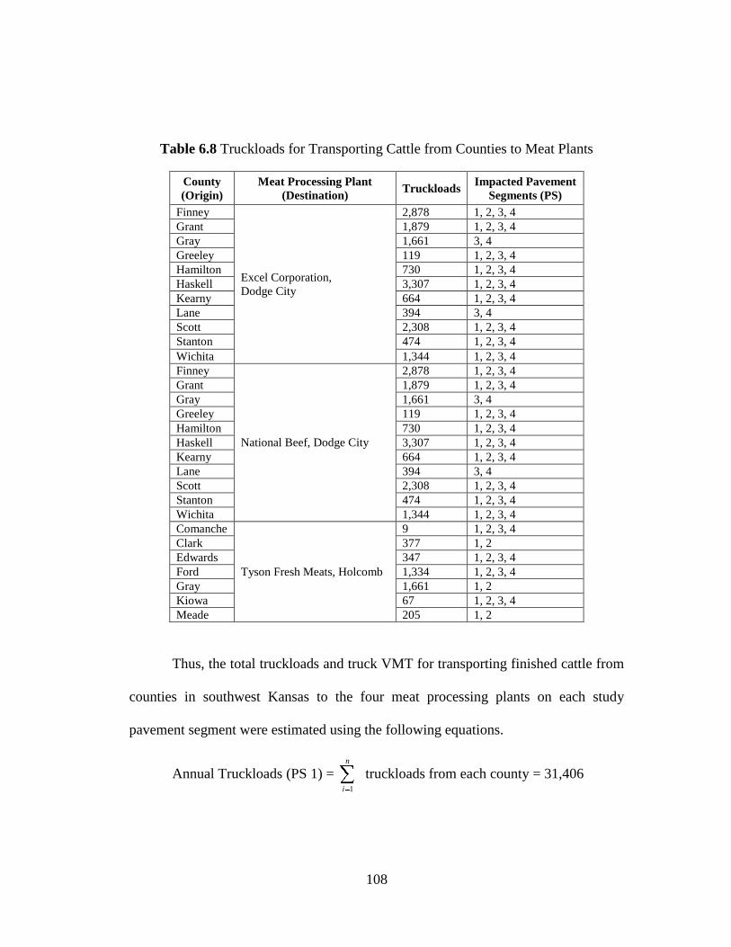
108
Table 6.8 Truckloads for Transporting Cattle from Counties to Meat Plants
County
(Origin)
Meat Processing Plant
(Destination) Truckloads
Impacted Pavement
Segments (PS)
Finney
Excel Corporation,
Dodge City
2,878 1, 2, 3, 4
Grant 1,879 1, 2, 3, 4
Gray 1,661 3, 4
Greeley 119 1, 2, 3, 4
Hamilton 730 1, 2, 3, 4
Haskell 3,307 1, 2, 3, 4
Kearny 664 1, 2, 3, 4
Lane 394 3, 4
Scott 2,308 1, 2, 3, 4
Stanton 474 1, 2, 3, 4
Wichita 1,344 1, 2, 3, 4
Finney
National Beef, Dodge City
2,878 1, 2, 3, 4
Grant 1,879 1, 2, 3, 4
Gray 1,661 3, 4
Greeley 119 1, 2, 3, 4
Hamilton 730 1, 2, 3, 4
Haskell 3,307 1, 2, 3, 4
Kearny 664 1, 2, 3, 4
Lane 394 3, 4
Scott 2,308 1, 2, 3, 4
Stanton 474 1, 2, 3, 4
Wichita 1,344 1, 2, 3, 4
Comanche
Tyson Fresh Meats, Holcomb
9 1, 2, 3, 4
Clark 377 1, 2
Edwards 347 1, 2, 3, 4
Ford 1,334 1, 2, 3, 4
Gray 1,661 1, 2
Kiowa 67 1, 2, 3, 4
Meade 205 1, 2
Thus, the total truckloads and truck VMT for transporting finished cattle from
counties in southwest Kansas to the four meat processing plants on each study
pavement segment were estimated using the following equations.
Annual Truckloads (PS 1) = n
i 1
truckloads from each county = 31,406
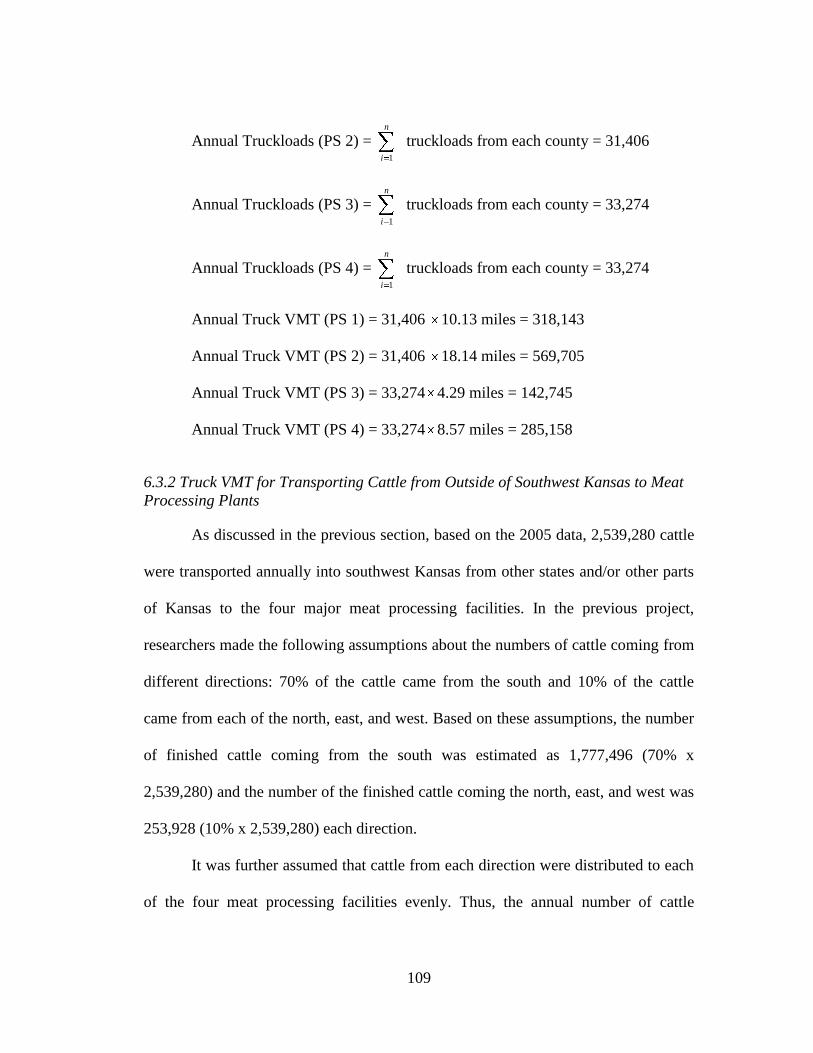
109
Annual Truckloads (PS 2) = n
i 1
truckloads from each county = 31,406
Annual Truckloads (PS 3) = n
i 1
truckloads from each county = 33,274
Annual Truckloads (PS 4) = n
i 1
truckloads from each county = 33,274
Annual Truck VMT (PS 1) = 31,406 10.13 miles = 318,143
Annual Truck VMT (PS 2) = 31,406 18.14 miles = 569,705
Annual Truck VMT (PS 3) = 33,274 4.29 miles = 142,745
Annual Truck VMT (PS 4) = 33,274 8.57 miles = 285,158
6.3.2 Truck VMT for Transporting Cattle from Outside of Southwest Kansas to Meat
Processing Plants
As discussed in the previous section, based on the 2005 data, 2,539,280 cattle
were transported annually into southwest Kansas from other states and/or other parts
of Kansas to the four major meat processing facilities. In the previous project,
researchers made the following assumptions about the numbers of cattle coming from
different directions: 70% of the cattle came from the south and 10% of the cattle
came from each of the north, east, and west. Based on these assumptions, the number
of finished cattle coming from the south was estimated as 1,777,496 (70% x
2,539,280) and the number of the finished cattle coming the north, east, and west was
253,928 (10% x 2,539,280) each direction.
It was further assumed that cattle from each direction were distributed to each
of the four meat processing facilities evenly. Thus, the annual number of cattle
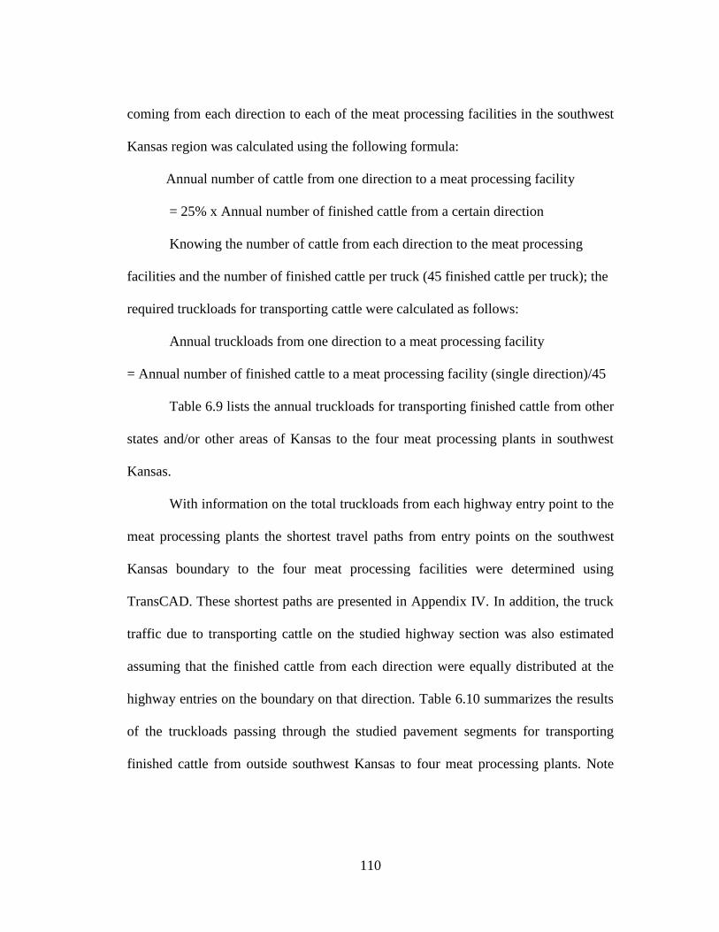
110
coming from each direction to each of the meat processing facilities in the southwest
Kansas region was calculated using the following formula:
Annual number of cattle from one direction to a meat processing facility
= 25% x Annual number of finished cattle from a certain direction
Knowing the number of cattle from each direction to the meat processing
facilities and the number of finished cattle per truck (45 finished cattle per truck); the
required truckloads for transporting cattle were calculated as follows:
Annual truckloads from one direction to a meat processing facility
= Annual number of finished cattle to a meat processing facility (single direction)/45
Table 6.9 lists the annual truckloads for transporting finished cattle from other
states and/or other areas of Kansas to the four meat processing plants in southwest
Kansas.
With information on the total truckloads from each highway entry point to the
meat processing plants the shortest travel paths from entry points on the southwest
Kansas boundary to the four meat processing facilities were determined using
TransCAD. These shortest paths are presented in Appendix IV. In addition, the truck
traffic due to transporting cattle on the studied highway section was also estimated
assuming that the finished cattle from each direction were equally distributed at the
highway entries on the boundary on that direction. Table 6.10 summarizes the results
of the truckloads passing through the studied pavement segments for transporting
finished cattle from outside southwest Kansas to four meat processing plants. Note
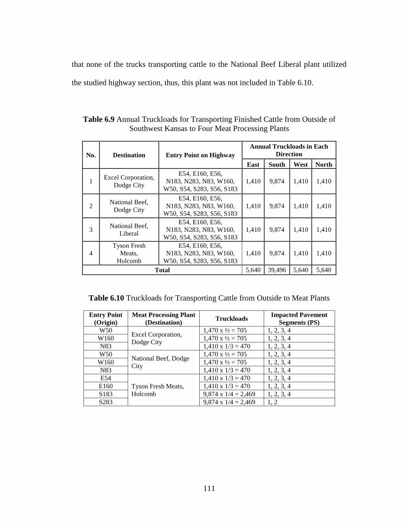
111
that none of the trucks transporting cattle to the National Beef Liberal plant utilized
the studied highway section, thus, this plant was not included in Table 6.10.
Table 6.9 Annual Truckloads for Transporting Finished Cattle from Outside of
Southwest Kansas to Four Meat Processing Plants
No. Destination Entry Point on Highway
Annual Truckloads in Each
Direction
East South West North
1 Excel Corporation,
Dodge City
E54, E160, E56,
N183, N283, N83, W160,
W50, S54, S283, S56, S183
1,410 9,874 1,410 1,410
2 National Beef,
Dodge City
E54, E160, E56,
N183, N283, N83, W160,
W50, S54, S283, S56, S183
1,410 9,874 1,410 1,410
3 National Beef,
Liberal
E54, E160, E56,
N183, N283, N83, W160,
W50, S54, S283, S56, S183
1,410 9,874 1,410 1,410
4
Tyson Fresh
Meats,
Holcomb
E54, E160, E56,
N183, N283, N83, W160,
W50, S54, S283, S56, S183
1,410 9,874 1,410 1,410
Total 5,640 39,496 5,640 5,640
Table 6.10 Truckloads for Transporting Cattle from Outside to Meat Plants
Entry Point
(Origin)
Meat Processing Plant
(Destination) Truckloads
Impacted Pavement
Segments (PS)
W50 Excel Corporation,
Dodge City
1,470 x ½ = 705 1, 2, 3, 4
W160 1,470 x ½ = 705 1, 2, 3, 4
N83 1,410 x 1/3 = 470 1, 2, 3, 4
W50 National Beef, Dodge
City
1,470 x ½ = 705 1, 2, 3, 4
W160 1,470 x ½ = 705 1, 2, 3, 4
N83 1,410 x 1/3 = 470 1, 2, 3, 4
E54
Tyson Fresh Meats,
Holcomb
1,410 x 1/3 = 470 1, 2, 3, 4
E160 1,410 x 1/3 = 470 1, 2, 3, 4
S183 9,874 x 1/4 = 2,469 1, 2, 3, 4
S283 9,874 x 1/4 = 2,469 1, 2
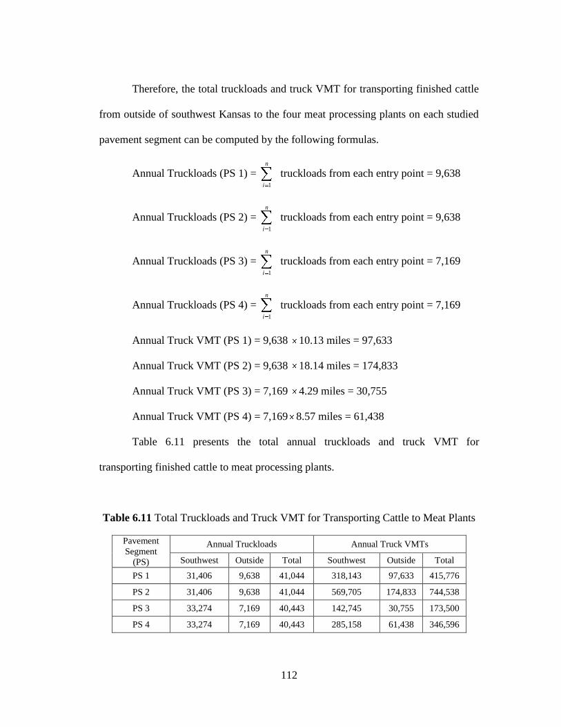
112
Therefore, the total truckloads and truck VMT for transporting finished cattle
from outside of southwest Kansas to the four meat processing plants on each studied
pavement segment can be computed by the following formulas.
Annual Truckloads (PS 1) = n
i 1
truckloads from each entry point = 9,638
Annual Truckloads (PS 2) = n
i 1
truckloads from each entry point = 9,638
Annual Truckloads (PS 3) = n
i 1
truckloads from each entry point = 7,169
Annual Truckloads (PS 4) = n
i 1
truckloads from each entry point = 7,169
Annual Truck VMT (PS 1) = 9,638 10.13 miles = 97,633
Annual Truck VMT (PS 2) = 9,638 18.14 miles = 174,833
Annual Truck VMT (PS 3) = 7,169 4.29 miles = 30,755
Annual Truck VMT (PS 4) = 7,169 8.57 miles = 61,438
Table 6.11 presents the total annual truckloads and truck VMT for
transporting finished cattle to meat processing plants.
Table 6.11 Total Truckloads and Truck VMT for Transporting Cattle to Meat Plants
Pavement
Segment
(PS)
Annual Truckloads Annual Truck VMTs
Southwest Outside Total Southwest Outside Total
PS 1 31,406 9,638 41,044 318,143 97,633 415,776
PS 2 31,406 9,638 41,044 569,705 174,833 744,538
PS 3 33,274 7,169 40,443 142,745 30,755 173,500
PS 4 33,274 7,169 40,443 285,158 61,438 346,596

113
6.4 Truck VMT for Transporting Meat to U.S. Customers
The processed meat (boxed beef) from each of the four meat processing
facilities is transported to various customers in the United States. In the previous
research, researchers assumed that processed meat was first distributed to customers
in six large cities in the U.S. including Atlanta, Chicago, Dallas, Los Angeles, New
York, and Phoenix. Then meat was distributed from these large cities to customers in
small satellite cities and towns. The researchers made this assumption based on the
following two reasons (Bai et al. 2007):
1. Based on interviews conducted during the site visits, researchers came to a
consensus that these six cities represented the biggest cities in the east, south,
west, and north directions from where the processed meat was mostly distributed
to other small cities and towns.
2. The same highways in the southwest Kansas region would be used to transport the
processed meat to customers in the U.S. even if the final destinations were not in
these six cities.
With the above assumption, the calculation of truck VMT on the studied
highway section for transporting meat to U.S. customers would be equivalent to the
determination of truck VMT generated by transporting meat to the six U.S. cities. To
calculate the VMT, the travel paths from the respective meat processing facilities to
the six cities were assigned to the major highways first using TransCAD software
based on the shortest path criteria. The results are listed in the maps and tables in
114
Appendix V. As indicated in the maps, only the travel path of transporting beef from
Tyson at Holcomb, KS to Dallas, TX passed through the studied pavement segments.
To estimate the truckloads for transporting beef from Tyson to Dallas, the
annual cattle slaughtered in this meat processing plant was estimated first. As
mentioned previously, based on the 2005 data an annual total of 6,260,330 cattle were
slaughtered in the four major meat processing plants in the southwest Kansas region.
Considering the similar scale of the four plants, it is reasonable to assume that a
quarter of the finished cattle were slaughtered in Tyson. Thus, the annual total
number of finished cattle slaughtered in Tyson in Dodge City is approximately equal
to 1, 565,083 (6,260,330 x 25%).
Based on results of previous research, the average weight of cattle at the time
of slaughtering is approximately 1,200 lbs. with about 720 pounds (60%) of red meat
and 480 pounds (40%) of byproducts (Bai et al. 2007). In addition, a truck can carry a
total of 42,000 pounds of boxed beef per load. Therefore, the annual quantity of red
meat originating at Tyson is:
Annual quantity of red meat from Tyson
= Total annual number of finished cattle coming to Tyson x 720 pounds
= 1,565,083 finished cattle x 720 pounds
= 1,126,859,760 pounds of red meat.
The annual number of truckloads for transporting boxed beef produced at Tyson can
be calculated as:
Annual Truckloads
115
= Annual quantity of red meat from Tyson / truck capacity
= 1,126,859,760 / 42,000
= 26,830 truckloads of boxed meat.
Thus, it was estimated that there were approximately 26,830 truckloads of
boxed beef produced by Tyson based on 2005 data. It was further assumed that the
quantity of boxed beef from each of the meat processing facilities (origins) was
equally distributed among the six large cities (destinations). In other words, about
16.67% (1/6 =16.67%) of the annual number of truckloads of boxed beef originating
at each meat processing facility was distributed to each of the six cities. Therefore,
the annual number of truckloads shipped from Tyson to Dallas, TX is as follows:
Annual number of truckloads from Tyson to Dallas, TX
= 16.67% x 26,830
= 4,473 truckloads of boxed meat.
Since these truckloads travel through all four studied pavement segments, the
annual truck VMTs on each segment are:
Annual Truck VMT on PS 1 = 4,473 10.13 miles = 45,312
Annual Truck VMT on PS 2 = 4,473 18.14 miles = 81,140
Annual Truck VMT on PS 3 = 4,473 4.29 miles = 19,189
Annual Truck VMT on PS 4 = 4,473 8.57 miles = 38,334
6.5 Truck VMT for Transporting Meat Byproducts
The meat byproducts produced at each of the four processing facilities
constitutes about 40% of the total live weight of the finished cattle. Based on previous
116
research results, about 50% of the byproducts produced are transported by rail and the
rest by truck (Bai et al. 2007). Some of the byproducts are exported to Mexico via
Dallas and East Asia via Phoenix and Los Angeles. Small amounts of the byproducts
such as technical (inedible) tallow and meat and bone meal are sent by trucks to local
feed yards to feed swine, chickens, and turkeys. Because the quantities of byproducts
sent to the feed yards are very small, previous researchers ignored the truck VMT for
transporting these byproducts.
In this research, Dallas, Los Angeles, and Phoenix were considered the only
destinations for transporting beef byproducts from the southwest Kansas region. The
travel paths on the major highways were determined using TransCAD software, as
shown in Appendix V. In Section 4.4 the annual number of finished cattle shipped to
the Tyson Fresh Meats plant is calculated as 1,565,083. Each finished cattle produces
about 480 lbs. (40%) of byproducts. Therefore, the annual quantity of byproducts
produced at Tyson is 751,239,840 (1,565,083 x 480) pounds.
Since 50% of byproducts are distributed by truck and the capacity of a truck is
42,000 lbs, the annual number of truckloads for transporting byproducts from Tyson
can be calculated as follows:
Annual truckloads for transporting byproducts from Tyson
= (50% x Annual quantity of byproducts at Tyson) / Truck capacity
= (50% x 751,239,840) / 42,000 lbs
= 8,943 truckloads.
117
Previous researchers suggested that it was reasonable to assume that 65% of
the byproducts transported by trucks were distributed south to Mexico via Dallas and
the rest (35%) were distributed to East Asia via Los Angeles and Phoenix with a half-
and-half split (Bai et al. 2007). Only the trips from Tyson to Dallas have impact on
the studied highway section. The annual number of truckloads from Tyson to Mexico
via Dallas is 5,813 (8,943 x 65%). Thus, the annual truck VMTs on the studied
pavement segments for transporting byproducts from Tyson Plant to Dallas can be
estimated as:
Annual Truck VMT on PS 1 = 5,813 10.13 miles = 58,886
Annual Truck VMT on PS 2 = 5,813 18.14 miles = 105,448
Annual Truck VMT on PS 3 = 5,813 4.29 miles = 24,938
Annual Truck VMT on PS 4 = 5,813 8.57 miles = 49,817
6.6 Summary
This chapter discussed the procedure and presented the results of annual truck
VMTs on the studied pavement segments generated by the processed beef and related
industries in the southwest Kansas. Based on the sequence of industries, the process
of estimating truck VMT was broken down into five steps including:
Truck VMT for transporting feeder cattle to feed yards in southwest Kansas;
Truck VMT for transporting feed grain to feed yards in southwest Kansas;
Truck VMT for transporting finished cattle to meat processing facilities in
southwest Kansas;
Truck VMT for transporting boxed beef to U.S. customers;
118
Truck VMT for transporting meat byproducts.
The total annual VMT generated by the beef and related industries in
southwest Kansas on the four pavement segments between Garden Cityand Dodge
City, Kansas are summarized in Table 6.12.
The numbers listed in Table 6.12 represent one-way trips. After unloading the
goods at destinations, trucks come back to their origins (roundtrip) with or without
return shipment. According to findings of previous research, most of the trucks come
back to their origins carrying goods such as tires, bagged fertilizer, groceries, and
bagged animal feed to minimize the shipping costs (Bai et al. 2007). However, the
percentage of the trucks with backhaul is not precisely known. Because of the limited
information, this study assumes that the return trucks (to their origins) cause the same
damage on the pavements as they did when shipping goods to their destinations.
Thus, the VMT listed in Table 6.12 needs to be doubled to account for return trips.
Table 6.13 shows the total daily & annual truck VMT of roundtrip shipments on the
studied pavement segments in the southwest Kansas.
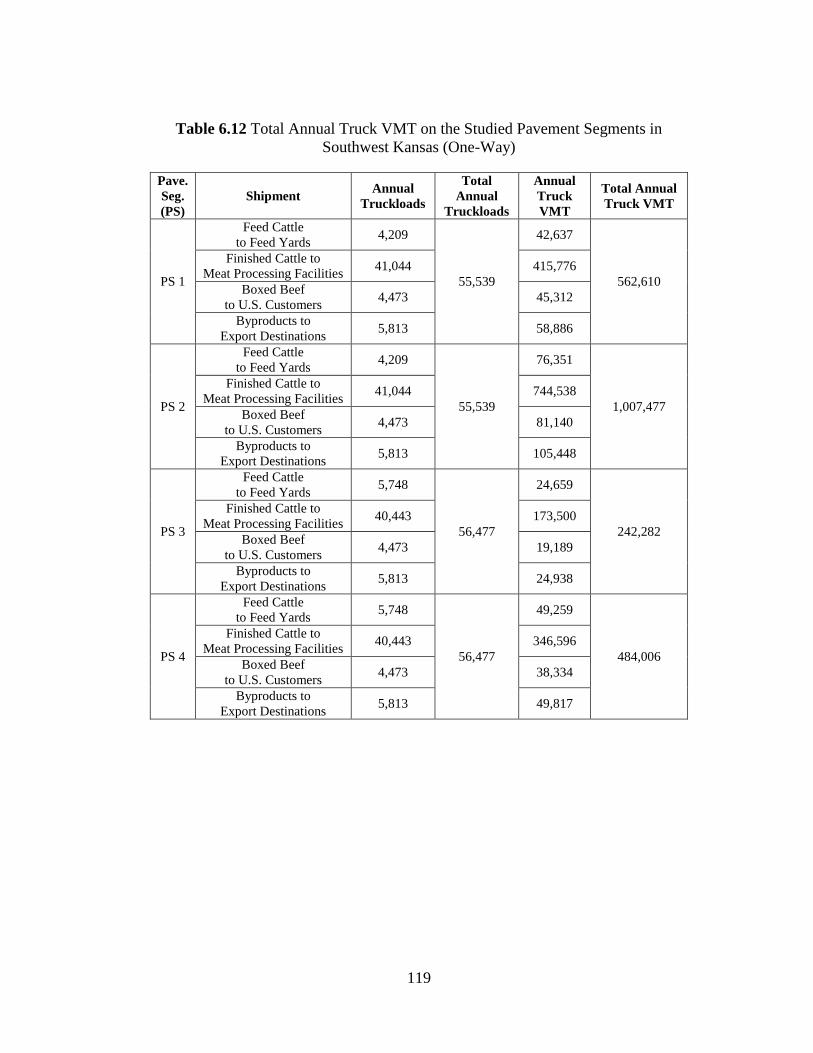
119
Table 6.12 Total Annual Truck VMT on the Studied Pavement Segments in
Southwest Kansas (One-Way)
Pave.
Seg.
(PS)
Shipment Annual
Truckloads
Total
Annual
Truckloads
Annual
Truck
VMT
Total Annual
Truck VMT
PS 1
Feed Cattle
to Feed Yards 4,209
55,539
42,637
562,610
Finished Cattle to
Meat Processing Facilities 41,044 415,776
Boxed Beef
to U.S. Customers 4,473 45,312
Byproducts to
Export Destinations 5,813 58,886
PS 2
Feed Cattle
to Feed Yards 4,209
55,539
76,351
1,007,477
Finished Cattle to
Meat Processing Facilities 41,044 744,538
Boxed Beef
to U.S. Customers 4,473 81,140
Byproducts to
Export Destinations 5,813 105,448
PS 3
Feed Cattle
to Feed Yards 5,748
56,477
24,659
242,282
Finished Cattle to
Meat Processing Facilities 40,443 173,500
Boxed Beef
to U.S. Customers 4,473 19,189
Byproducts to
Export Destinations 5,813 24,938
PS 4
Feed Cattle
to Feed Yards 5,748
56,477
49,259
484,006
Finished Cattle to
Meat Processing Facilities 40,443 346,596
Boxed Beef
to U.S. Customers 4,473 38,334
Byproducts to
Export Destinations 5,813 49,817
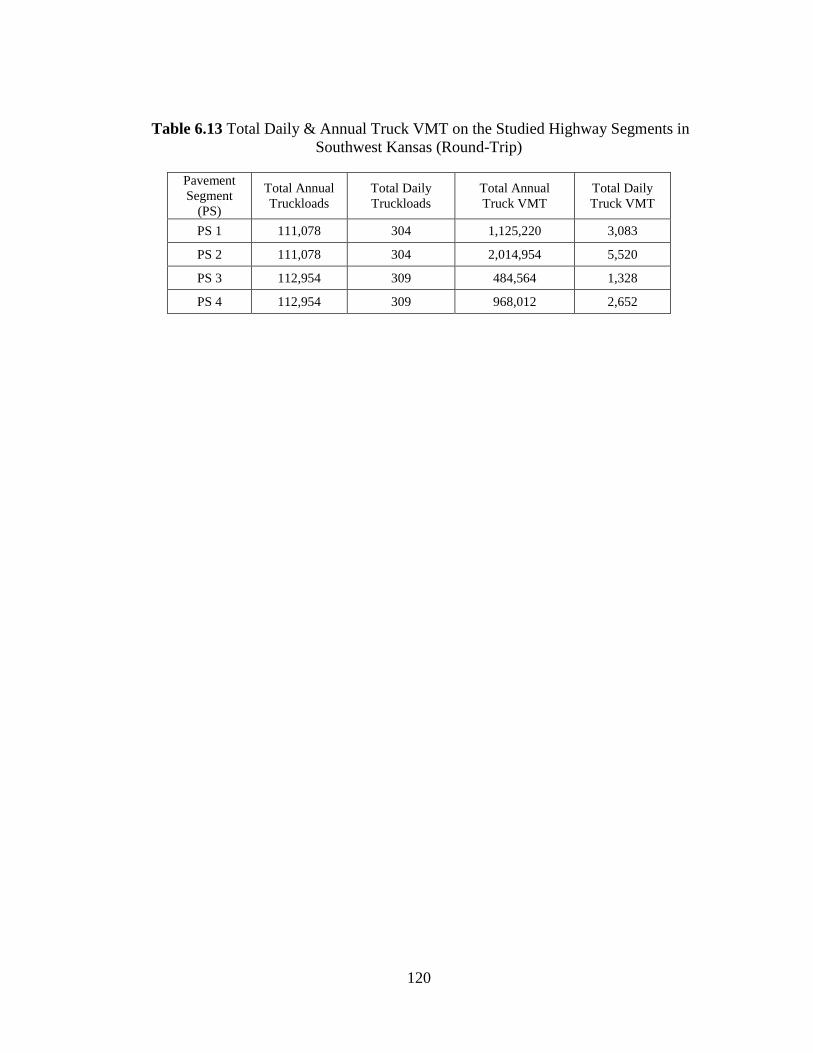
120
Table 6.13 Total Daily & Annual Truck VMT on the Studied Highway Segments in
Southwest Kansas (Round-Trip)
Pavement
Segment
(PS)
Total Annual
Truckloads
Total Daily
Truckloads
Total Annual
Truck VMT
Total Daily
Truck VMT
PS 1 111,078 304 1,125,220 3,083
PS 2 111,078 304 2,014,954 5,520
PS 3 112,954 309 484,564 1,328
PS 4 112,954 309 968,012 2,652
121
Chapter 7 Conclusions and Recommendations
7.1 Conclusions
Kansas is one of the leaders in meat production in the United States. In the
southwest Kansas region there are more than three hundred feed yards and several of
the biggest meat processing plants in the nation. Heavy trucks (e.g., tractor-trailers)
have been used primarily for transporting processed meat, meat byproducts, grain,
and other related products. With the continuous growth of these industries, there will
be more trucks on highways transporting meat and meat-related products in southwest
Kansas.
The high truck VMT generated by the beef processing and related industries
in southwest Kansas causes noteworthy damage to Kansas highway pavements,
which in turn leads to more frequent maintenance actions and ultimately more traffic
delays and congestion. A systematical analysis of heavy-truck-related highway
maintenance costs will be beneficial for the selection of cost-effective transportation
modes for the meat processing and related industries in southwest Kansas. It also
helps KDOT to assess highway maintenance needs and to set up maintenance
priorities. Meanwhile, the analysis results will be valuable for the determination of
reasonable user costs.
To thoroughly study the pavement damage caused by beef industry-related
truck traffic, the researcher first conducted a comprehensive literature review to

122
obtain relevant background knowledge. Second, data for truckloads generated by the
beef and related industries and the studied pavement data were determined. Third,
based on these data, the total truck VMT and annual equivalent single axle loads
(ESALs) associated with the industries for the studied pavement segments were
calculated. Fourth, the unit cost per ESAL was computed and adjusted by the truck
traffic PSR loss factor. Finally, the total damage costs associated with processed beef
and related industries on the studied pavement segments were estimated by
multiplying the unit cost per ESAL by the total annual ESALs generated by the
industries.
In this study, the researcher used a systematic pavement damage estimation
procedure that synthesized several existing methodologies including HERS and
AASHTO methods. The procedure utilized in this research provides a practical
approach to estimate pavement damage costs attributed to truck traffic associated
with certain industries on specific pavement segments. Using this approach, general
pavement damage costs associated with heavy trucks could also be estimated if the
truck traffic volume and predominant truck types were known.
The study results showed that, for the 41-mile-long highway section, US
50/400 from Garden City to Dodge City, the total highway damage cost associated
with processed meat related industries was estimated as $71,019 per year, or $1,727
per mile. The damage cost per truck per mile was approximately $0.02. If the same
truck traffic was presented on all major highways in southwest Kansas (1835 miles),
123
the total damage cost attributed to the processed meat and related industries would be
$3,169,045 per year.
It was estimated that, every day, 309 trucks on the studied highway section
were generated by the processed meat and related industries. This is about one third
of the truck traffic on the traffic count map provided by KDOT. This number may be
underestimated for the reasons that follow. First, the researcher assumed that grain
was shipped by train to elevators and then distributed by trucks only through local
roads instead of major highways such as US 50/400. Second, the travel routes
analyses were based on the major highway network in Kansas and used only shortest-
path criterion that assumes all driver decisions are rational and are made with good
information at the travel times. These assumptions may be biased and may result in
underestimating the truck traffic volume.
The accuracy of the study results may be affected by some other factors. For
example, it was noted during data collection that a certain proportion of the trucks
were frequently overloaded to lower their shipping costs. However, because of the
limited information, this study assumed that all trucks had the standard weight. Other
assumptions such as shipping origin and destination locations, shipping proportional
distributions, and truck route selections may also lead to a certain degree of
estimation errors. To minimize these errors, more accurate and comprehensive data
on the truck traffic and beef and related industries would be necessary.
124
7.2 Recommendations
Based on the study results, the researcher offers the following
recommendations.
In this study, the highway damage that was caused by the truck traffic generated by
beef and related industries in southwest Kansas was assessed. The analysis helps
traffic engineers and other stakeholders to understand the truck travel paths and
highway pavement maintenance costs attributable to the beef industries in southwest
Kansas. There is a need to estimate the highway damage caused by other vital
regional industries so that the causal relations between the highway maintenance
costs and these industries can be better understood. This knowledge would be useful
for highway project prioritization and project funding allocations. The analysis results
would be a good reference for determination of reasonable user costs for different
industries.
Meat processing and related industries have been predicted to continue growing in the
future. Truck volumes for these industries were projected to increase from 10% to
20% on highways in the southwest Kansas region from 2007 to 2015. In addition, the
growth of other related businesses in the study area, including dairy farms, milk
processing plants, and ethanol plants, will contribute to the increase of truck traffic.
The large amount of truck VMTs would cause rapid deterioration of Kansas
highways, not to mention an increase in the crash rate. Poor pavements constrain
travel speeds and cause damages for all motor vehicles traveling on them. This
deterioration not only affect traveler safety and comfort, but increase vehicle-
125
operating costs such as maintenance and depreciation. To mitigate these impacts,
railroads need to be considered as an alternative to truck transportation. The
researcher recommends the study of the feasibility and economic benefits of
increased use of rail transportation for beef and related industries. There is a need to
study the rail infrastructure in southwest Kansas and to determine if it is feasible as an
alternative transportation mode and how existing business could use it. Location
studies are also needed to select the best places to establish new businesses (e.g.,
dairy and ethanol) to better utilize all transportation modes available in the southwest
Kansas area.
Because of data limitations, this study could not estimate the net costs of
pavement damage caused by beef-related truck traffic. In a future study,
highway revenues generated from fuel taxes and other user fees should be
estimated and subtracted from highway maintenance costs to yield the net
costs of highway pavement damage due to beef and related industries in
southwest Kansas.
126
References
Guidelines for Pavement Management Systems. American Association of State Highway
and Transportation Officials. Washington, D.C.: AASHTO, 1990.
Guide for Design of Pavement Structures. American Association of State Highway and
Transportation Officials.) GDPS-4. Washington, D.C., AASHTO.
American Association of State Highway and Transportation Officials. (2001). Pavement
Management Guide, Washington, D.C.: AASHTO, 1993.
Babcock, M. W., J.L. Bunch, J. Sanderson, and J. Witt. Economic Impacts of Railroad
Abandonment on Rural Kansas Communities. Topeka, KS: Kansas Department of
Transportation, 2003.
Bai, Y., P. Oslund, T. Mulinazzi, S. Tamara, C. Liu, M.M. Barnaby, C.E. and Atkins.
Transportation Logistics and Economics Of The Processed Meat And Related
Industries In Southwest Kansas. Topeka, KS: Kansas Department of Transportation,
2007.
Boile, M., K. Ozbay, and P. Narayanan. Infrastructure Costs Attributable to Commercial
Vehicles. Trenton, NJ: New Jersey Department of Transportation, 2001.
Chow, M. H., M.W. Babcock, and L.O. Sorenson. ―The Changing Logistics Structure for
Grain Marketing: A Case Study of Export Wheat in Northwest
Kansas.‖Transportation Journal 24.3(1985): 37-46.
Comerford, J., G. Greaser, H. Moore, J. Harper. ―Beef Backgrounding Production.‖ Penn
State University Cooperative Extension, Agricultural Alternative. 2001.
<http://agalternatives.aers.psu.edu/livestock/beefbackgrounding/beef_backgrounding.
pdf> (accessed July 25, 2006).
Darter, M. I. Requirements for Reliable Predictive Pavement Models. Transportation
Research Record 766. Washington, D.C.: TRB, 1980.
Dhuyvetter, K. ―Projected Budgets, Livestock & Meat: Budgets, Kansas
AGMANAGER.INFO.‖ KSU: Kansas State Research and Extension, 2006.
Elseifi, M. A., I.L. Al-Qadi, P.J. Yoo, and I. Janajreh. ―Quantification of Pavement
Damage Caused by Dual and Wide-Base Tires.‖ Transportation Research Record
1940. Washington, D.C.: Transportation Research Board, 2005.
127
Eusebio, V. and S. Rindom. ―Grain Transportation Service Demand Projections for
Kansas: 1995 and Beyond.‖ Bureau of Rail Affairs. Kansas Department of
Transportation (KDOT), 1990.
Federal Highway Administration. ―Pavement and Road Surface Management for Local
Agencies.‖ In Participant’s Manual. Washington, D.C.: FHWA, (1995).
Freeman, T. E. and T.M. Clark, T. M. ―Performance of Pavements Subject to Higher
Truck Weight Limits in Virginia.‖ Transportation Research Record 1806.
Washington D.C.: Transportation Research Board, 2002.
―Glossary of Truck Terms, 2007 Light Commercial Vehicle Body Application Guide,
GM Fleet and Commercial.‖ General Motors. (2006).
<http://www.gmfleet.com/gmfleetjsp/share/commTruckGuide/Glossary.pdf>,
(accessed Aug. 8, 2006).
Griffin, D. ―Water Quality for Beef Cattle.‖ University of Nebraska – Great Plains
Veterinary Educational Center, Clay Center, NE. 2002.
<http://72.14.203.104/u/UNL1?q=cache:qHaTHs64z1oJ:gpvec.unl.edu/bqa/NCBQA_
TrainingSupportFiles/WQReview.doc+water+quality+for+beef+cattle&hl=en&gl=us
&ct=clnk&cd=1&ie=UTF-8> (accessed August 2, 2006).
Haas, R., W.R. Hudson, and J. Zaniewski. Modern Pavement Management. Malabar, FL:
Krieger Publishing Company, 1994.
Hajek, J.J., S.L. Tighe, and B.G. Hutchinson. ―Allocation of Pavement Damage Due to
Trucks Using a Marginal Cost Method‖. Transportation Research Record 1613.
Washington D.C.: Transportation Research Board, 1998.
Haper, W. V. and K. Majidzadeh. ―Utilization of Expert Opinion in the Two Pavement
Management Systems.‖ Presentation at the 70th
Annual Meeting of the Transportation
Research Board. Washington, D.C., 1991.
Huang, Y. H. Pavement Analysis and Design, 2nd
edition. Upper Saddle River, NJ:
Prentice Hall, 2009.
Karamihas, S. M., T.D. Gillespie, R.W. Pereva, and S.D. Kohn. ―Guidelines for
Longitudinal Pavement Profile Measurement.‖ NCHRP 434. Washington, D. C.:
Transportation Research Board, 1999.
Kulkarni, R. B. and R.W. Miller. ―Pavement Management Systems – Past, Present, and
Future.‖ Transportation Research Record 1853. Washington D.C.: Transportation
Research Board, 2003.
128
Lenzi, J.C., E. Jessup, and K.L. Casavant. Prospective Estimates for Road Impacts in
Eastern Washington From a Drawdown of the Lower Snake River. Eastern
Washington Intermodal Transportation Study. Working Paper Number 2. Washington
State Department of Transportation, 1996.
Lytton, R. L. ―Concepts of Pavement Performance Prediction and Modeling.‖ Vol. 2.
Proceedings from the Second North American Conference on Managing Pavements.
Toronto, Canada: Ontario Ministry of Transportation, 1987.
Martin, T. C. ―Estimating Heavy Vehicle Road Wear Costs for Bituminous-Surfaced
Arterial Roads.‖ Journal of Transportation Engineering. ASCE. 128.2 (2002): 103-
110.
McCracken, M. ―Financial Terms.‖ TeachMeFinance. 2005.
<http://teachmefinance.com/Financial_Terms/p.html> (accessed Jul. 17, 2005).
Mrad, N., M. El-Gindy, and W. Kenis. Effects of Wheel-Load Spatial Repeatability on
Road Damage: A Literature Review. Federal Highway Administration, 1998.
Distress Identification manual for the Long-Term Pavement Performance Project.
National Research Council. NRC, SHRP-P-338. Washington, D.C.: Strategic
Highway Research Program, 1993.
Owusu-Ababio, S. and R. Schmitt. Effects of Heavy Loading on Wisconsin’s Concrete
Pavements.Madison, WI: Wisconsin Department of Transportation, 2005.
Petz, J. and J. Heiman. 2005. Personal Interview. Irsik & Doll (I&D), Cimarron, KS.
Phares, B. M., T. Wipf, and H. Ceylan. Impacts of Overweight Implements of Husbandry
on Minnesota Roads and Bridges. St. Paul, MN: Minnesota Department of
Transportation, 2004.
Roadway Express. Shipper‘s Info – Trailer Dimensions. 2005.
<http://www.roadway.com/shippers/glossaryG-L.html> (accessed July 17, 2005).
Pollan, M. ―Power Steer.‖ New York Times Magazine, March 31, 2002, 44.
Roberts, F. L., A. Saber, A. Ranadhir, and X. Zhou. Effects of Hauling Timer, Lignite
Coal, and Coke Fuel on Louisiana Highways and Bridges. Louisiana Department of
Transportation and Development, 2005.
129
Ramaswamy, R. and M. Ben-Akiva. Estimation of Highway Pavement Deterioration
from In-Service Data. Transportation Research Record 1272. Washington, D.C.:
Transportation Research Board,1990.
Russell, E. R., M.W. Babcock and C. Mauler. ―A Methodology for Determining Road
Damage Due to Railroad Branchline Abandonment.‖ 1996 Semi-sesquicentennial
Transportation Proceedings, Kansas Department of Transportation, Topeka, Kansas.
Salgado, R. and D. Kim. Effects of Heavier Truck Loadings and Super-Single Tires on
Subgrades, Indianapolis, IN: Indiana Department of Transportation, 2002.
Sebaaly, P.E., R. Siddharthan and D. Huft. ―Impact of Heavy Vehicles on Low Volume
Roads.‖ Transportation Research Record 1819. Washington D.C.: Transportation
Research Board, 2002.
Shahin, M. Y. Pavement management for Airports, Roads, and Parking Lots. New York,
NY, 1994.
Smith, W., F. Finn, R. Kulkarni et al. Bayesian Methodology for Verifying
Recommendations to Minimize Asphalt Pavement Distress. NCHRP Report 213.
Washington, D.C.: TRB, 1979.
Sullivan, W. G., E.M. Wicks and L.T. Luxhoj. Engineering Economy. 12th
Edition. Upper
Saddle River, NJ: IIE Transactions, 2003.
Tolliver, D., K. Andres and B. Lindamood. Washington Rail Impact Analysis: Executive
Summary. Washington State Department of Transportation,1994.
Tolliver, D. and HDR Engineering Inc. Benefits of Rail Freight Transportation in
Washington: A Multimodal Analysis, Appendix C. Washington State Department of
Transportation. 2000.
Transportation Research Board. Calibration of Response-Type Road Roughness
measuring Systems. NCHRP Report 228. Washington, D.C.: TRB, 1980.
Transportation Research Board. Current Practices in Determining Pavement Condition.
NCHRP Synthesis 203. Washington, D.C.: TRB, 1994.
United States Department of Agriculture (USDA). ―2005 Kansas Farm Facts.‖ National
Agricultural Statistics Service. 2005.
<http://www.nass.usda.gov/ks/ffacts/2005/pdf/general.pdf> ( accessed July 25, 2006).
130
United States Department of Agriculture (USDA) (2006a). ―Cattle.‖ National
Agricultural Statistics Service, <http://www.nass.usda.gov/ks/catshp/cattle06. pdf>
(accessed July 25, 2006).
United States Department of Agriculture (USDA). ―Kansas Data – Cattle and Calves.‖
National Agricultural Statistics Service – Quick Stats, (2006b).
<http://www.nass.usda.gov/Statistics_by_State/Kansas/index.asp> (accessed August
7, 2006).
United States Department of Agriculture (USDA).―U.S. Cattle Supplies and
Dispositions.‖ National Agricultural Statistics Service, (2006c).
<http://usda.mannlib.cornell.edu/usda/nass/Catt//2000s/2006/Catt-03-24-
2006_Special%20Report.pdf > (accessed July 25, 2006).
United States Department of Labor (USDL). ―Producer Price Indexes.‖ 2007.
<http://www.bls.gov/ppi/> (accessed Oct. 15, 2007).
United States Department of Transportation and Federal Highway Administration.
Instructor’s Manual Participant’s Workbook Visuals. 1998.
United States Department of Transportation. Comprehensive Truck Size and Weight
Study: Issues and Background. Report No. FHWA-PL-00-029, Federal Highway
Administration (FHWA), U.S. Department of Transportation (US DOT), August,
2000.
United States Department of Transportation. Comprehensive Truck Size and Weight
Study, Report No. 2, 1996.
<http://www.fhwa.dot.gov/reports/tswstudy/Vol2-Chapter3.pdf>, (accessed August,
2000).
Washington State Department of Transportation (WSDOT). The WSDOT Pavement
Guide Interactive, 2003. <http://training.ce.washington.edu/WSDOT/> (accessed
May 3, 2007).
Wood, C. The Kansas Beef Industry. Lawrence, KS: The Regents Press of Kansas, 1980.
Wright, P. H. and K.K. Dixon. Highway Engineering. 7th
Ed. Hoboken, NJ: 2004.
131
Appendixes
Appendix I: Shortest Paths from County Centroids to Feed Yards in the Respective
County
Appendix II: Shortest Paths from Entry Points in the Boundary to County Centroids
Appendix III: Shortest Paths from County Centroids to Four Meat Processing Plants in
Southwest Kansas
Appendix IV: Shortest Paths from Entry Points to Four Meat Processing Plants in
Southwest Kansas
Appendix V: Shortest Paths from Four Meat Processing Plants to U.S. Cities
Appendix VI: Producer Price Index Detailed Data (1981-2007) (USDL 2007)

132
Appendix I: Shortest Paths from County Centroids to Feed Yards in the Respective
County
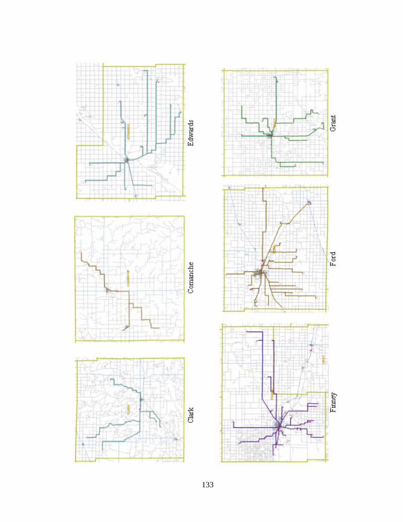
133
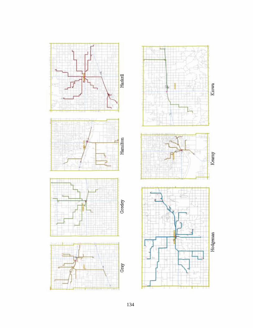
134
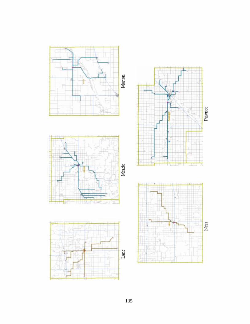
135
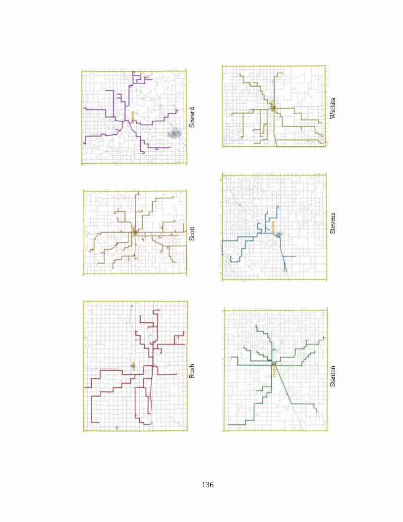
136
137
Appendix II: Shortest Paths from Entry Points in the Boundary to County Centroids
Figure II.1 Shortest Paths from Entry Points in the East Boundary to County Centroids
Table II.1 Highway Mileages from Entry Points in the East Boundary to County Centroids
Figure II.2 Shortest Paths from Entry Points in the North Boundary to County Centroids
Table II 2 Highway Mileages from Entry Points in the North Boundary to County Centroids
Figure II.3 Shortest Paths from Entry Points in the West Boundary to County Centroids
Table II.3 Highway Mileages from Entry Points in the West Boundary to County Centroids
Figure II.4 Shortest Paths from Entry Points in the South Boundary to County Centroids
Table II.4 Highway Mileages from Entry Points in the South Boundary to County Centroids
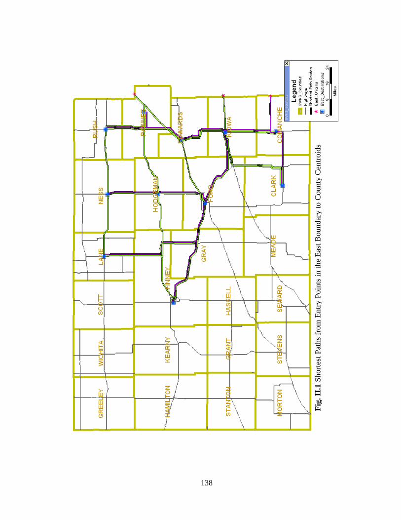
138
Fig
. II
.1 S
hort
est
Pat
hs
from
Entr
y P
oin
ts i
n t
he
Eas
t B
oundar
y t
o C
ounty
Cen
troid
s
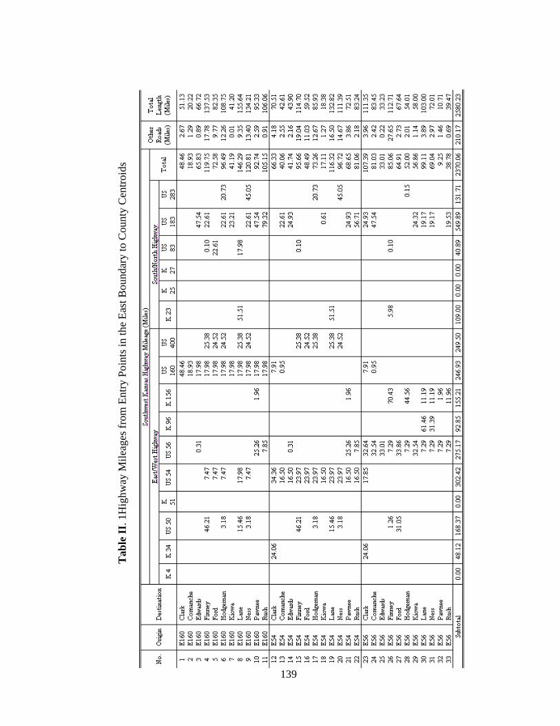
139
Tab
le I
I. 1
Hig
hw
ay M
ilea
ges
fro
m E
ntr
y P
oin
ts i
n t
he
Eas
t B
oundar
y t
o C
ounty
Cen
troid
s
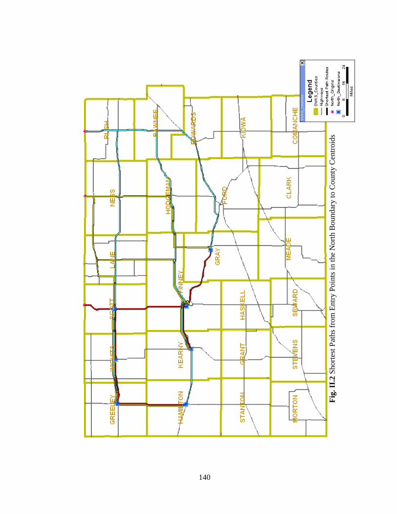
140
Fig
. II
.2 S
hort
est
Pat
hs
from
Entr
y P
oin
ts i
n t
he
Nort
h B
oundar
y t
o C
ounty
Cen
troid
s
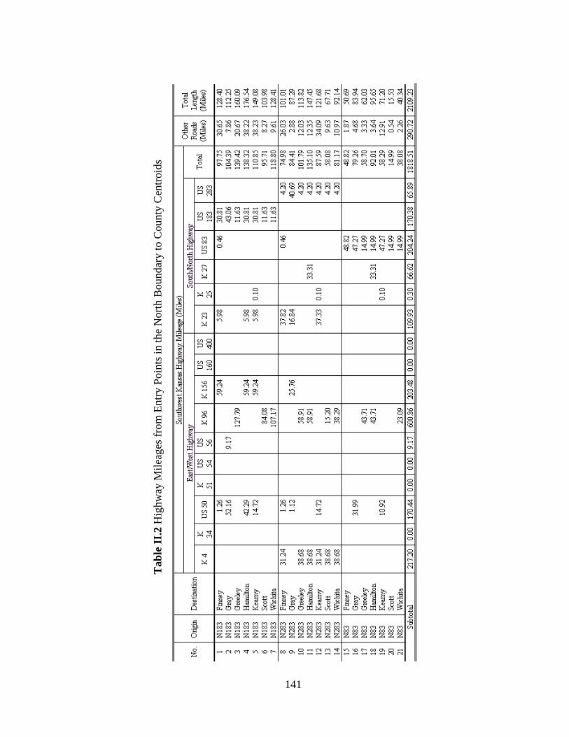
141
Tab
le I
I.2 H
ighw
ay M
ilea
ges
fro
m E
ntr
y P
oin
ts i
n t
he
Nort
h B
oundar
y t
o C
ounty
Cen
troid
s
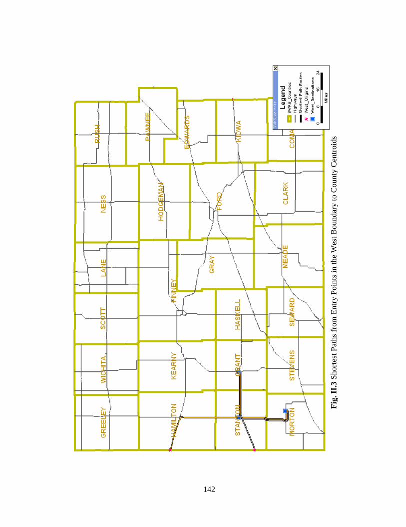
142
Fig
. II
.3 S
hort
est
Pat
hs
from
Entr
y P
oin
ts i
n t
he
Wes
t B
oundar
y t
o C
ounty
Cen
troid
s
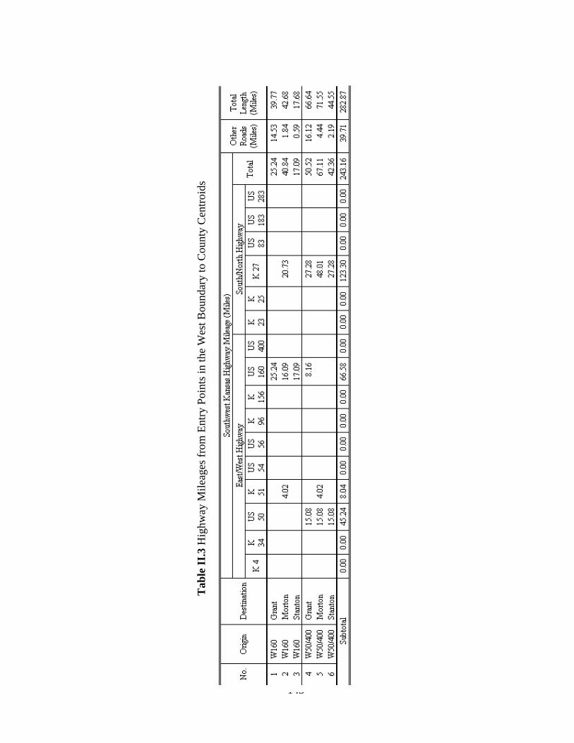
143
Tab
le I
I.3 H
ighw
ay M
ilea
ges
fro
m E
ntr
y P
oin
ts i
n t
he
Wes
t B
oundar
y t
o C
ounty
Cen
troid
s
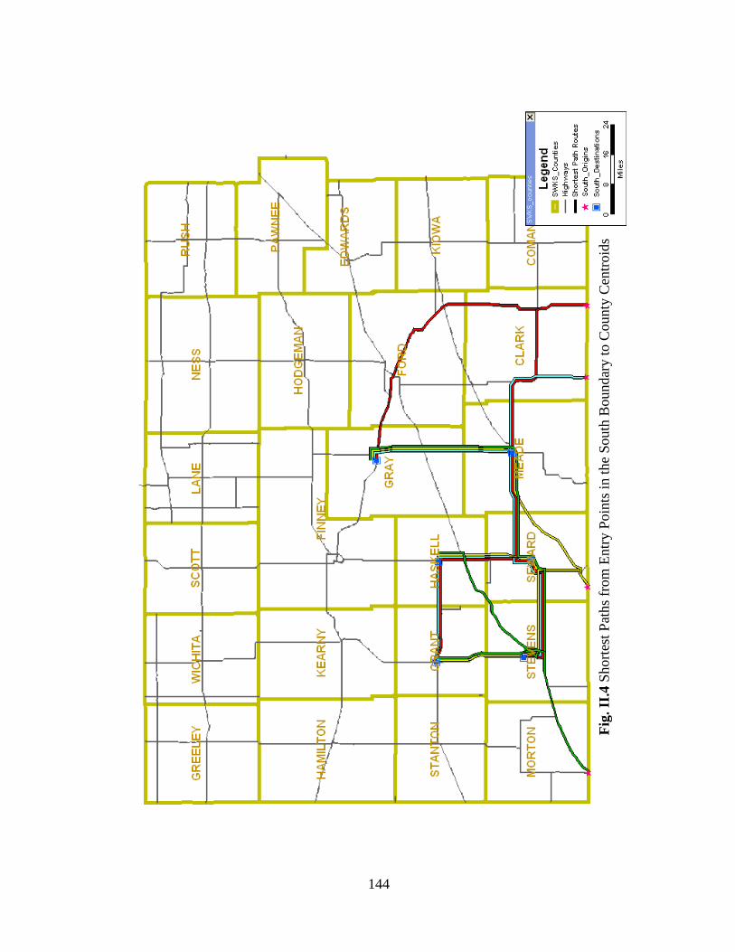
144
Fig
. II
.4 S
hort
est
Pat
hs
from
Entr
y P
oin
ts i
n t
he
South
Boundar
y t
o C
ounty
Cen
troid
s
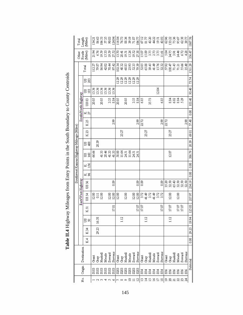
145
Tab
le I
I.4 H
ighw
ay M
ilea
ges
fro
m E
ntr
y P
oin
ts i
n t
he
South
Boundar
y t
o C
ounty
Cen
troid
s
146
Appendix III: Shortest Paths from County Centroids to
Four Meat Processing Plants in Southwest Kansas
Figure III.1 Shortest Paths from County Centroids to Excel Corporation
Table III. 1 Highway Mileage from County Centroids to Excel Corporation
Figure III.2 Shortest Paths from County Centroids to National Beef in Dodge City
Table III.2 Highway Mileage from County Centroids to National Beef in Dodge City
Figure III.3 Shortest Paths from County Centroids to National Beef in Liberal
Table III.3 Highway Mileage from County Centroids to National Beef in Liberal
Figure III.4 Shortest Paths from County Centroids to Tyson
Table III.4 Highway Mileage from County Centroids to Tyson and Summary
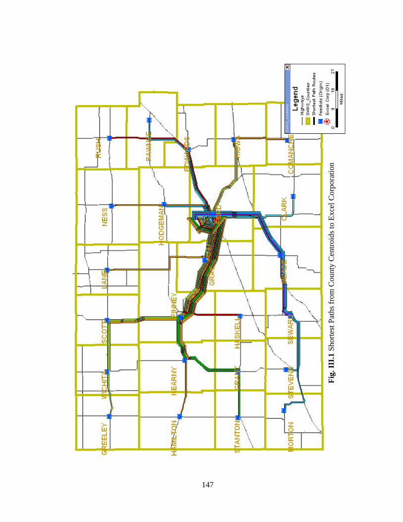
147
Fig
. II
I.1 S
hort
est
Pat
hs
from
County
Cen
troid
s to
Exce
l C
orp
ora
tion
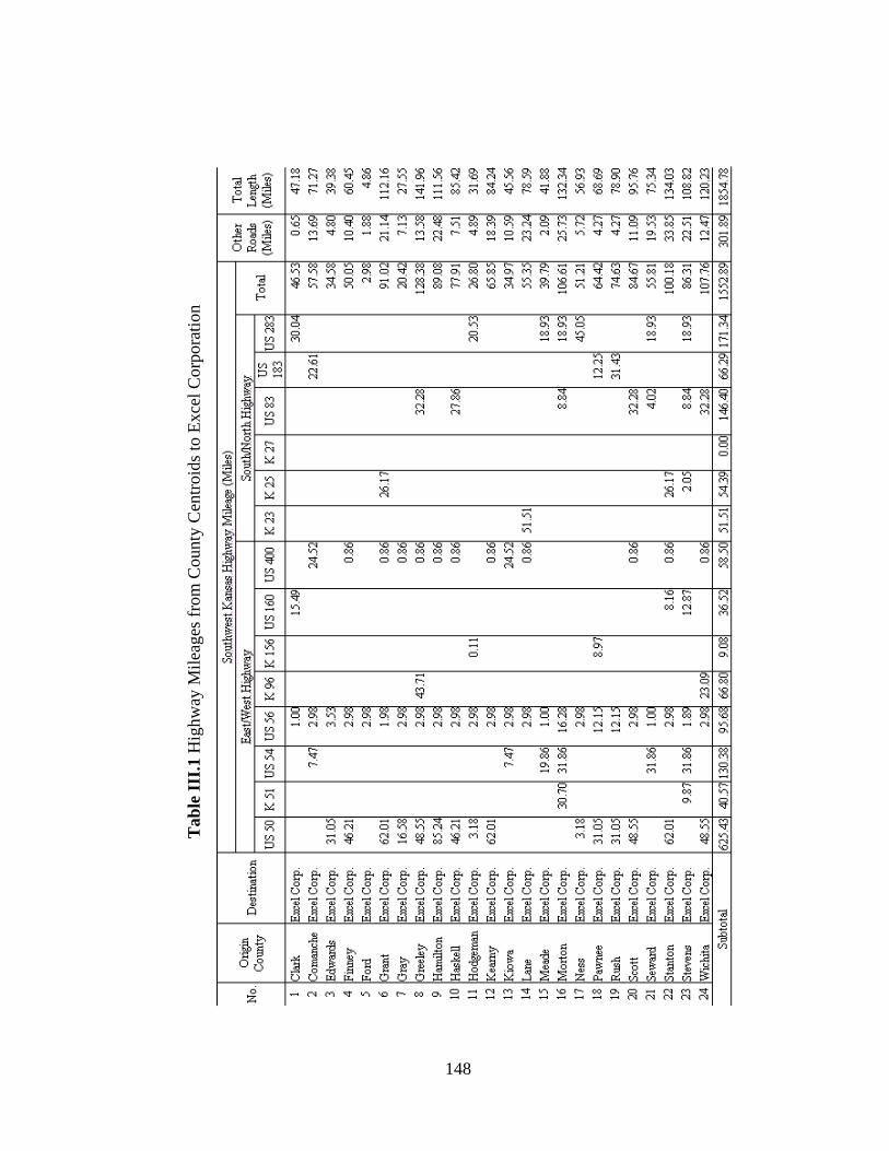
148
Tab
le I
II.1
Hig
hw
ay M
ilea
ges
fro
m C
ounty
Cen
troid
s to
Exce
l C
orp
ora
tion
Hig
hw
ay M
ilea
ges
fro
m C
oun
ty C
entr
oid
s to
Ex
cel
Co
rpo
rati
on
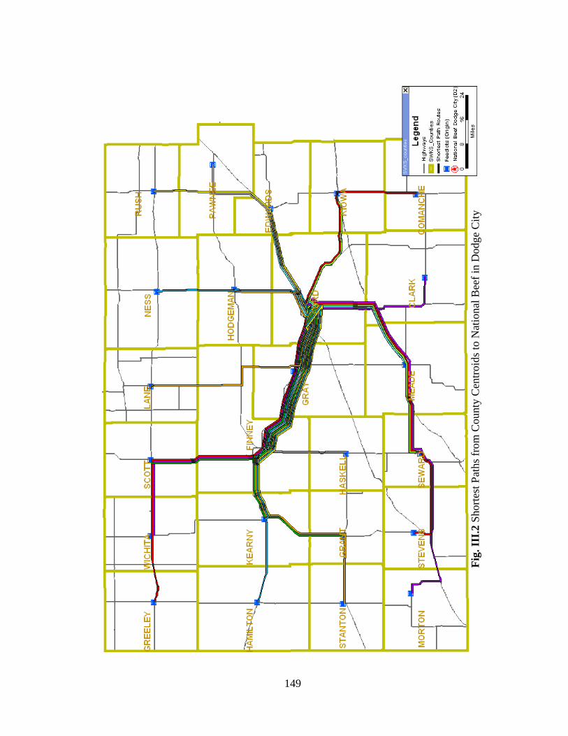
149
Fig
. II
I.2 S
hort
est
Pat
hs
from
County
Cen
troid
s to
Nat
ional
Bee
f in
Dodg
e C
ity
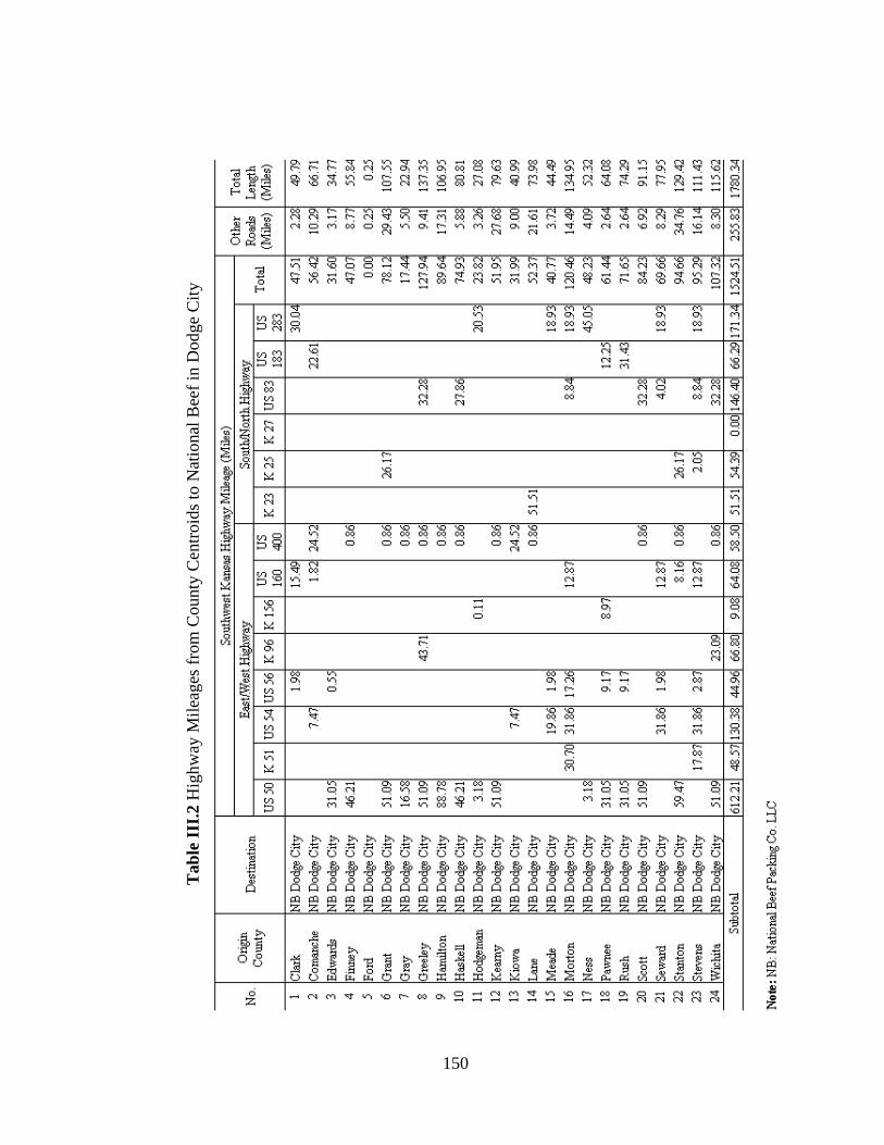
150
Tab
le I
II.2
Hig
hw
ay M
ilea
ges
fro
m C
ounty
Cen
troid
s to
Nat
ional
Bee
f in
Dodge
Cit
y
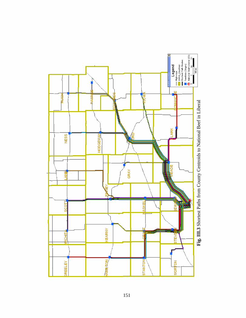
151
Fig
. II
I.3 S
hort
est
Pat
hs
from
County
Cen
troid
s to
Nat
ional
Bee
f in
Lib
eral
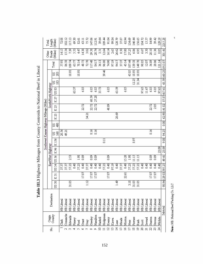
152
Tab
le I
II.3
Hig
hw
ay M
ilea
ges
fro
m C
ounty
Cen
troid
s to
Nat
ional
Bee
f in
Lib
eral
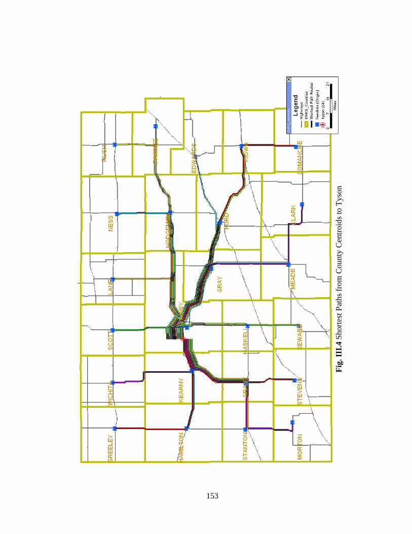
153
Fig
. II
I.4 S
hort
est
Pat
hs
from
County
Cen
troid
s to
Tyso
n
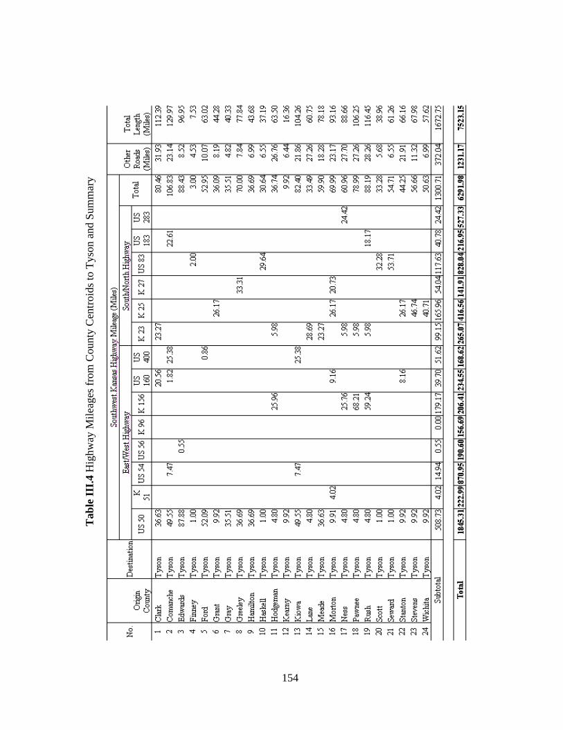
154
Tab
le I
II.4
Hig
hw
ay M
ilea
ges
fro
m C
ounty
Cen
troid
s to
Tyso
n a
nd S
um
mar
y
155
Appendix IV: Shortest Paths from Entry Points to
Four Meat Processing Plants in Southwest Kansas
Figure IV.1 Shortest Paths from East Entry Points to Four Meat Processing Plants
Table IV.1 Highway Mileages from East Entry Points to Four Meat Processing Plants
Figure IV.2 Shortest Paths from South Entry Points to Four Meat Processing Plants
Table IV.2 Highway Mileages from South Entry Points to Four Meat Processing Plants
Figure IV.3 Shortest Paths from West Entry Points to Four Meat Processing Plants
Table IV.3 Highway Mileages from West Entry Points to Four Meat Processing Plants
Figure IV.4 Shortest Paths from North Entry Points to Four Meat Processing Plants
Table IV.4 Highway Mileages from North Entry Points to Four Meat Processing Plants
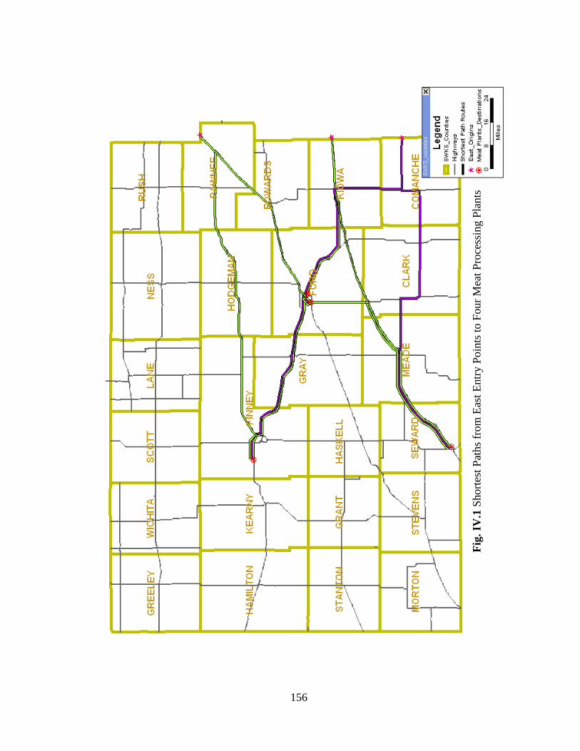
156
Sh
ort
est
Pat
hs
fro
m E
ast
En
try
Po
ints
to
Fo
ur
Mea
t P
roce
ssin
g P
lan
ts
Fig
. IV
.1 S
hort
est
Pat
hs
from
Eas
t E
ntr
y P
oin
ts t
o F
our
Mea
t P
roce
ssin
g P
lants
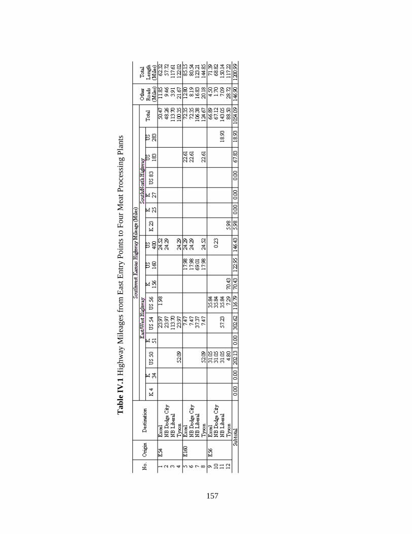
157
Fig
ure
VII
I.1
: S
ho
rtes
t P
ath
s fr
om
Ea
st E
ntr
y P
oin
ts t
o F
ou
r M
eat
Pro
cess
ing
Pla
nts
Tab
le I
V.1
Hig
hw
ay M
ilea
ges
fro
m E
ast
Entr
y P
oin
ts t
o F
our
Mea
t P
roce
ssin
g P
lants
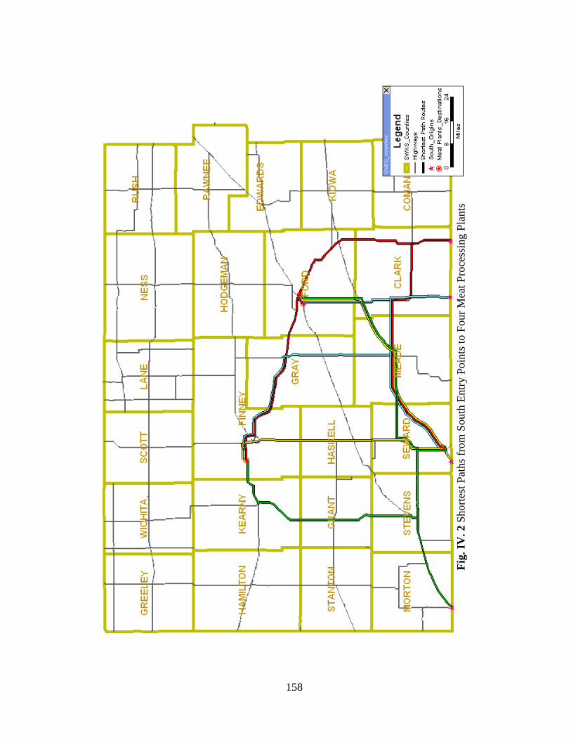
158
Fig
. IV
. 2 S
hort
est
Pat
hs
from
South
Entr
y P
oin
ts t
o F
our
Mea
t P
roce
ssin
g P
lants
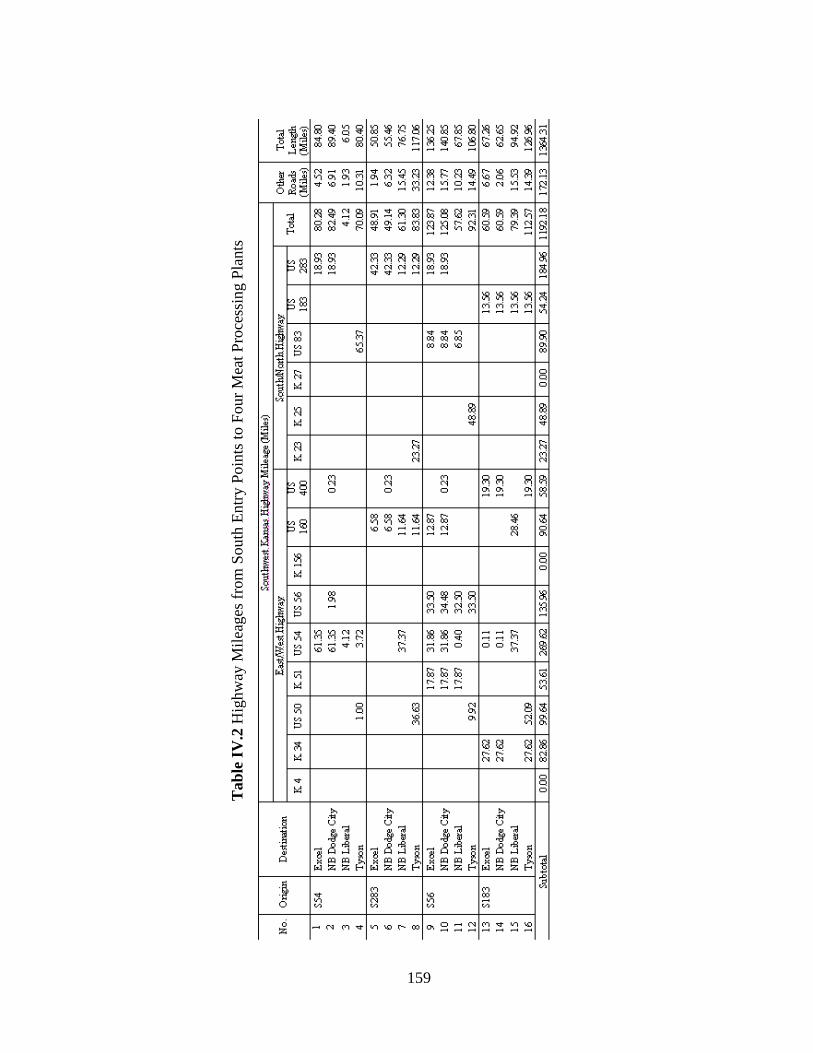
159
Tab
le I
V.2
Hig
hw
ay M
ilea
ges
fro
m S
outh
Entr
y P
oin
ts t
o F
our
Mea
t P
roce
ssin
g P
lants
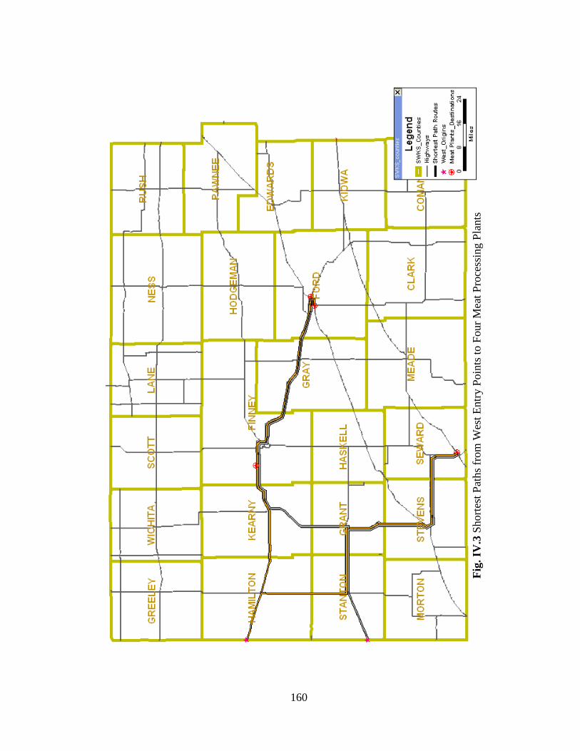
160
Fig
. IV
.3 S
hort
est
Pat
hs
from
Wes
t E
ntr
y P
oin
ts t
o F
our
Mea
t P
roce
ssin
g P
lants
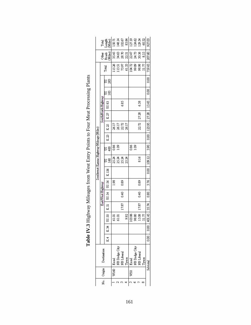
161
Tab
le I
V.3
Hig
hw
ay M
ilea
ges
fro
m W
est
Entr
y P
oin
ts t
o F
our
Mea
t P
roce
ssin
g P
lants
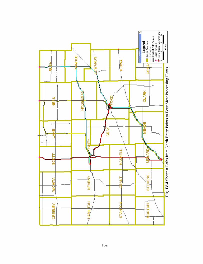
162
Fig
. IV
.4 S
hort
est
Pat
hs
from
Nort
h E
ntr
y P
oin
ts t
o F
our
Mea
t P
roce
ssin
g P
lants
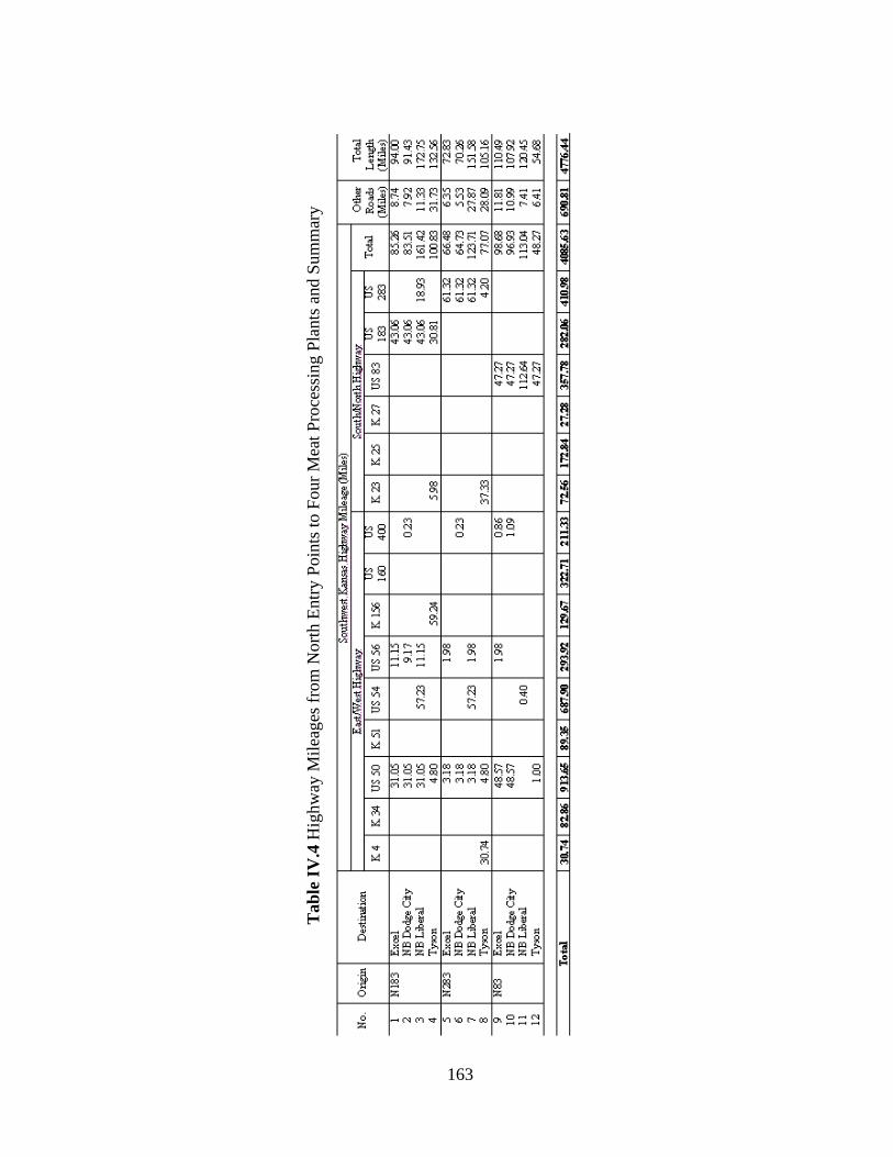
163
Tab
le I
V.4
Hig
hw
ay M
ilea
ges
fro
m N
ort
h E
ntr
y P
oin
ts t
o F
our
Mea
t P
roce
ssin
g P
lants
and S
um
mar
y
164
Appendix V: Shortest Paths from Four Meat Processing Plants to U.S. Cities
Figure V.1 Map of Meat Processing Plants (Origins) and Six US cities (Destinations)
Figure V.2 Shortest Paths from Four Meat Processing Plants to Six US Cities
Figure V.3 Shortest Paths from Four Meat Processing Plants to Six US Cities (Kansas Part)
Table V.1 Highway Mileages from Four Meat Processing Plants to Six US Cities
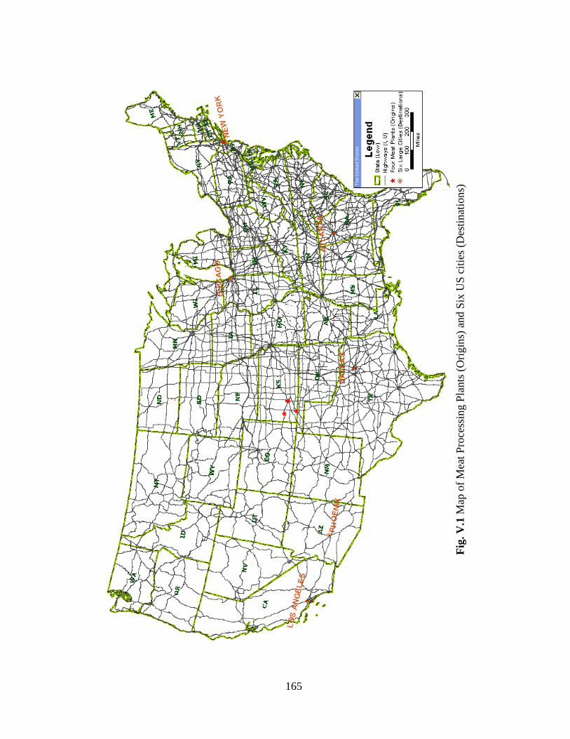
165
Fig
. V
.1 M
ap o
f M
eat
Pro
cess
ing P
lants
(O
rigin
s) a
nd S
ix U
S c
itie
s (D
esti
nat
ions)
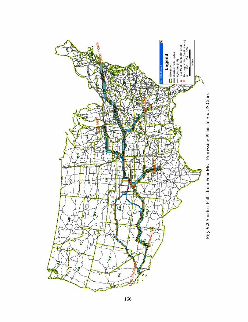
166
Fig
. V
.2 S
hort
est
Pat
hs
from
Four
Mea
t P
roce
ssin
g P
lants
to S
ix U
S C
itie
s
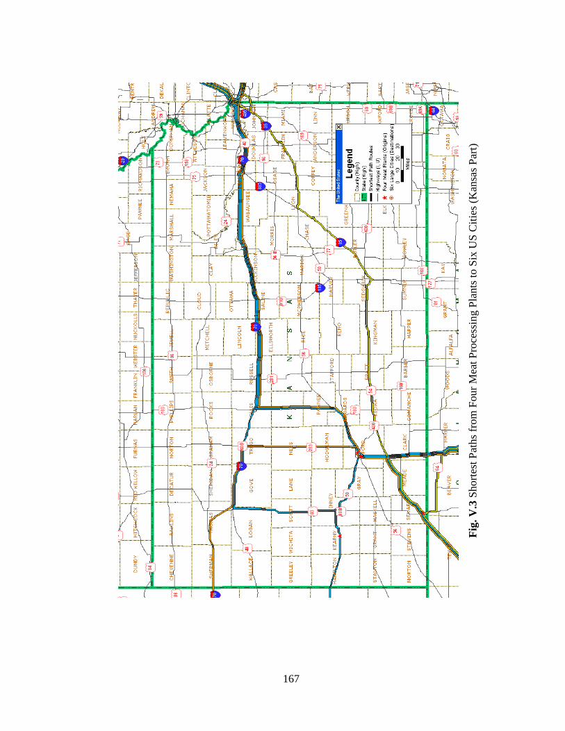
167
Fig
. V
.3 S
hort
est
Pat
hs
from
Four
Mea
t P
roce
ssin
g P
lants
to S
ix U
S C
itie
s (K
ansa
s P
art)
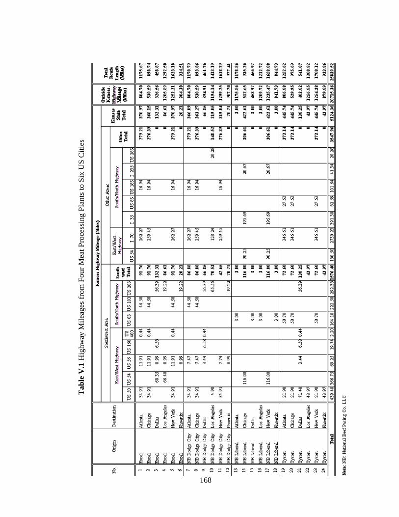
168
Tab
le V
.1 H
ighw
ay M
ilea
ges
fro
m F
our
Mea
t P
roce
ssin
g P
lants
to S
ix U
S C
itie
s

169
Appendix VI: Producer Price Index Detailed Data (1981-2007) (USDL 2007)
Table VI.1 PPI Data for Materials and Components for Construction (1981-2007)
Table VI.2 PPI Data for Construction Machinery and Equipment (1981-2007)
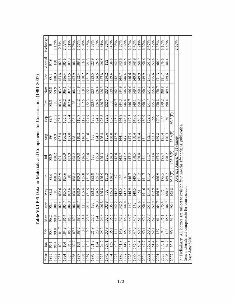
170
Tab
le V
I.1
PP
I D
ata
for
Mat
eria
ls a
nd C
om
ponen
ts f
or
Const
ruct
ion (
1981
-2007)
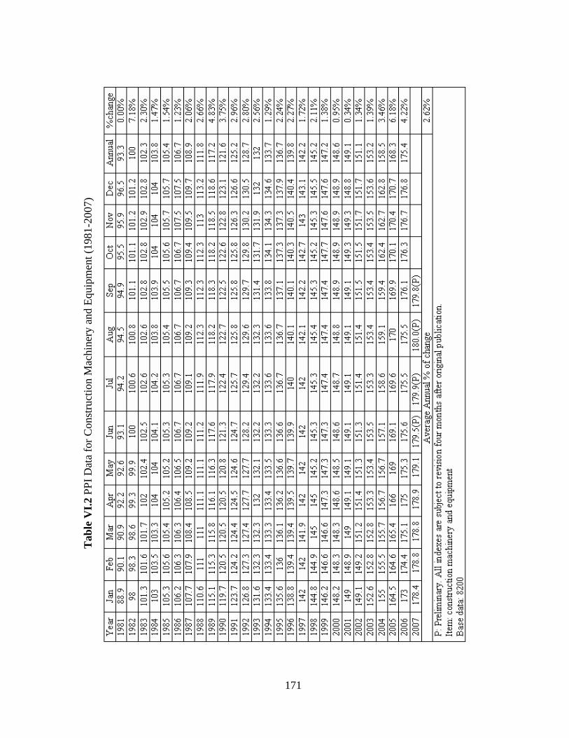
171
Tab
le V
I.2 P
PI
Dat
a fo
r C
onst
ruct
ion M
achin
ery a
nd E
quip
men
t (1
981
-20
07)

172