Estimating Demand Elasticities Using

Nonlinear Pricing

Christina Marsha

aDepartment of Economics, 515 Brooks Hall, Terry College of Business, University ofGeorgia, Athens, GA 30602

Abstract

Nonlinear pricing is prevalent in industries such as health care, public utili-ties, and telecommunications. However, this pricing scheme introduces biasinto estimating elasticities for welfare analysis or policy changes. I develop alocal elasticity estimation method that uses nonlinear price schedules to iso-late consumers’ expenditure choices from selection and simultaneity biases.This method improves over previous approaches by using commonly-availableobservational data and requiring only a single general monotonicity assump-tion. Using claims-level data on health insurance with two nonlinearities, Iam able to measure two separate elasticities, and find elasticity declines from-0.26 to -0.09 by the second nonlinearity. These estimates are then used tocalculate moral hazard deadweight loss. This method enables estimation ofmany policies with nonlinear pricing which previous tools could not address.

Keywords: Elasticity, nonlinear, health insurance, moral hazardJEL Classification: D40, I11, C14

IParticular thanks to Patrick Bajari and Robert Town. I also thank W. David Bradford,Meghan Busse, Meg Henkel, Thomas Holmes, Ginger Jin, Willard Manning, Amil Petrin,Connan Snider, Kevin Wiseman, and Thomas Youle for helpful comments.

∗Email: clmarsh@uga.edu, Tel:(706) 542-3668, Fax:(706) 542-3376

Preprint submitted to Elsevier June 21, 2014

1. Introduction

Demand elasticities are important to policy makers for designing cost-sharing and calculating welfare in sectors such as health insurance, publicutilities, and telecommunications. However, pricing is commonly nonlinear inthese sectors, for example in deductibles in health insurance, tiered pricing inpublic utilities, and contracts with usage allowances in telecommunications.1

Nonlinear pricing contributes to efficient plan design, but complicates esti-mation of elasticities for several reasons. First, the price a consumer facesis a function of quantity; consumers must pass a certain level of spendingto reach a new price level. Second, selection bias occurs when an unobserv-able factor, such as health status or preferences for high versus low data use,pushes a consumer above or below the nonlinearity. Using observable vari-ables such as age to proxy may not reduce bias, since unobservable healthstatus is likely correlated with age. It is difficult to get rid of this selectionbias without experimental data or an exogenous shock, both of which areempirically rare.

In this paper, I present a method to calculate elasticity in the presence ofnonlinear pricing in consumer contracts. This method uses the nonlinearityitself to control for bias by taking advantage of the discontinuous change inprice across the nonlinearity, while controlling for the underlying distributionof individual unobserved characteristics. This method has very general datarequirements and uses only one minimally restrictive assumption: that theexpenditure of interest must be increasing in the unobserved preference char-acteristic. I then apply this method to a private health insurance claims-leveldataset with two nonlinearities. In addition to providing an updated healthexpenditure demand elasticity, my results also are novel because I am able toestimate elasticities at different points on the same demand curve. Identifica-tion uses the nonparametric estimation framework of Matzkin (2003). Thismethod uses the same key insight as Bajari et al. (2010), but here I focuson individual consumer contracts rather than provider contracts. Consumershave less precise control over health expenditures given health status thanBajari et al. (2010) find using provider charges by hospitals over a diversity of

1See for example, Reiss and White (2002), Herriges and King (1994), Maddock et al.(1992) in electricity, Szabo (2010) and Diakite et al. (2009) in water and development, andGrubb and Osborne (2012), Reiss and White (2006), Seim and Viard (2011), and Huang(2008) in cell phone markets.

2

expense categories. Besides the novel setting of consumer contracts, apply-ing this method to health insurance contracts estimates health expenditureelasticities which are used to design contracts and make welfare predictionsof insurance expansions. This paper is able to measure elasticities in twoseparate regions, which is informative since demand for health care likelychanges along its typically skewed spending distribution.

The goal of the method is to generate local elasticities within a contractwith nonlinear pricing. The method is aimed at policy applications suchas understanding consumer behavior in certain regions, or how changingpricing schedules might effect the distribution of spending, given a particularconsumer contract design.

The “gold standard” of elasticity estimation is experimental data. Thebest example in the health industry is the RAND Health Insurance Experi-ment (HIE), which began in 1971 and was conducted over 15 years (Manninget al. (1987) and Newhouse (1993)). The RAND HIE avoided selection biasby randomizing patients into health plans’ pricing schedules. While excellentfor reducing selection bias, experimental data is extremely costly in terms ofboth time and money and is difficult to replicate. In addition, the resultsfrom the HIE best apply to the same population type and insurance frame-work of the HIE. This estimation method can be used on more specific pop-ulations of interest to policy makers or on new insurance structures. Sincethe RAND HIE, exogenous shocks or natural experiments have been usedto control for simultaneity and selection bias. Cherkin et al. (1989) use theintroduction of office visit copayments for government employees to create aquasi-experimental price change with which to measure elasticity. Selby et al.(1996) use a similar technique taking advantage of a copayment introductionfor emergency room visits in a large HMO. In measuring price response moregenerally, Doyle and Almond (2011) find a substantial increase in mother’slength of stay due to better insurance coverage around a policy treatment forchildren born just before and just after midnight. These natural experimentsare difficult for policy makers to use regularly, however, because they rely onunique exogenous changes.

Eichner (1998) and Kowalski (2010) create a natural experiment in thepresence of a deductible when an unexpected injury exogenously pushes othernon-injured family members into a different pricing zone. Using a two-periodutility model, Duarte (2012) also uses an unforseen accident instrument onChilean data to reveal how elasticities vary by income and demographics.However, unexpected injury in a deductible structure is hard to replicate

3

in pharmaceutical or public utilities data, for example. The method pre-sented here is accessible to policy makers outside of the health plan familydeductible, a useful tool given the prevalence of nonlinear pricing in manyother sectors.

Previous methods also estimate one elasticity over the whole range ofexpenditures. In health expenditures especially, distributions are commonlyskewed, with a large proportion of consumers spending small amounts anda long tail of high spending consumers. Tiered pricing structures are oftencreated precisely because different groups of consumers exist. Telecommuni-cations users who end up near usage allowance limits are using bandwidthdifferently than low bandwidth users, i.e. using email versus video stream-ing. Estimating one elasticity over an entire range may mask heterogeneityof elasticity values along the distribution. An advantage of this method topolicy makers is that is provides a local estimate of elasticity around currentpricing points - those very areas that policy makers and insurance adminis-trators may be modifying.

The main intuition of this estimation uses the kink in the price scheduleat the nonlinearity. Selection bias exists because agents on either side of thenonlinearity face different prices, but are also different on an unobservabledimension such as health status or preferences for bandwidth use. In thispaper’s setting of a deductible, patients who surpass the deductible face alower price for care, but also likely had more health shocks. However, themarginal price of an additional unit of care remains constant on each side,but changes suddenly at the nonlinearity. Identification is off the fact thatmarginal price is constant within the estimation regions, but the distributionof health status changes along the estimation window. Using the differencesin the density of final spending before and after the nonlinearity allows us toisolate the change in spending due only to prices.

Identification is based on Matzkin (2003). The only condition that musthold is that final expenditure is strictly increasing in the individual unob-served characteristics that induce expenditure. For example, if an individualhas a higher preference for bandwidth use, his final expenditure on band-width usage will be higher than an individual with a lower preference foruse. For health insurance, this unobserved characteristic measure will beable to capture a more general ranking of health than diagnosis codes orself-reported health status. The unobserved characteristics are essentially alatent error term. Given this condition and using Matzkin (2003) I am ableto proxy the distribution of unobservable characteristics using the percentiles

4

of final expenditures.Given both final expenditures and the estimated relative values of the un-

observed characteristics, the method uses local linear regression to measurehow expenditure increases for an increase in the unobserved characteristic.I calculate this slope on each side of the nonlinearity. The final elastic-ity estimate is the difference between the two slopes as they approach thenonlinearity and the threshold enrollee, thus controlling for selection and si-multaneity bias while isolating the response due solely to price. I then plugthis price response into an elasticity formula which includes the price levelat the nonlinearity to calculate final elasticity.

I apply this method to a detailed claims-level dataset for an employer-sponsored Consumer Driven Health Plan (CDHP). This plan was chosenbecause it has two nonlinear pricing points. Although baseline implementa-tion of this method only requires individual-level final expenditure and thepricing structure associated with the expenditures, the greater detail in mydata allows me to perform several robustness checks of the method with ob-servable variables. I find elasticity estimates of -0.26 in lower expenditureranges compared with -0.09 in higher spending ranges. These estimates areslightly above and below the RAND HIE estimate of -0.22, which was not alocal estimate, but instead estimated over a broad range of spending. Previ-ous literature uses elasticities as an indicator of moral hazard in insurance. Itake my elasticity estimate one step further to measure moral hazard dead-weight loss by calculating the counterfactual choices the elasticity predicts.The deadweight loss from full-coverage insurance is approximately 20 percentof final expenditures less than $1,000.

This paper builds on the elasticity estimation literature in health, but alsointo a more general nonlinear estimation literature. Maximum likelihood ap-proaches such as in Gary and Hausman (1978) and Hausman (1985) requirespecific distributional assumptions, whereas the method outlined here usesnonparametric estimation and requires only one strict monotonicity assump-tion. Other tax applications, such as Blomquist and Newey (2002) requiresubstantial variation in prices across sample observations, which is less likelyto hold for pricing in the sectors above than for taxes. Recent work by Saez(2010) and Chetty et al. (2013) also look at nonlinearities in the EITC taxcode. Saez finds evidence consistent with changing labor hours in responseto changes in the tax code, but finds that the most pronounced changescan be attributed to tax evasion. The method here is related, but has theadvantage that the main condition of monotonicity links the outcome of in-

5

terest and unobserved characteristics more flexibly, which allows for the lackof distinct bunching cited by Saez. Aron-Dine et al. (2012) also highlightthe highly nonlinear environment of health insurance. The authors examineexpenditure response to health insurance price within a year, to address theproblem that a patient’s price changes along his distribution of expenditure.This work highlights the difficulties of calculating an elasticity using onlyone price over a large range of values. This question of forward-looking ormyopic behavior is not of first-order concern in this paper, however, becausethis method targets those just below or just above a deductible – individu-als with relatively similar probabilities of reaching a post-deductible price.Those individuals well beyond a nonlinearity are not in the scope of thisestimation method or local elasticity.

This paper has three contributions. First, I present a new method formeasuring elasticities with minimal distributional or modeling assumptions.The method has commonly attainable data requirements and can be appliedto consumer contracts. Second, this method is based on a common featurewhich previously introduced bias in estimation, but can now be used in avariety of sectors. Using nonlinearities means this method is most useful forlocal elasticities along expenditure distributions. Finally, I use this method toestimate elasticities for an employer-sponsored health insurance plan over twodifferent areas of the spending distribution to measure changes in elasticityand then measure the deadweight loss of moral hazard.

The rest of the paper proceeds as follows: Section 2 sets up a generalmodel of expenditure choice. Section 3 lays out the estimation framework,Section 4 describes the data, and Section 5 discusses the elasticity results.Section 6 describes the moral hazard estimation and results. Section 7 con-cludes.

2. General Model of Health Expenditure

This section lays out a model of a patient’s health expenditure choicewithin an insurance plan with nonlinear pricing. The goal of the model is togenerate predictions on the relationship between the underlying distributionof health shocks of a population and the population’s health expenditurechoices. I will use the model to compare the distribution of final expendituresin the pre-deductible region versus the post-deductible region. The modelpresented here is similar to the framework in Huang and Rosett (1973), andgenerates the same reduced form predictions as the approaches in Manning

6

et al. (1987), and Newhouse et al. (1980). In what follows, the patient ischoosing his annual expenditure in dollars after having already chosen hisinsurance plan.2

To place this model in the example of a deductible, consider patientsvisiting a physician over the course of the year in response to various healthshocks. A patient may benefit from multiple visits to the physician, with acost for each visit. As the number of visits increases, the patient crosses thedeductible and enters a higher coverage region. As the patient’s marginalcost of a visit changes, the patient adjusts the frequency of his physicianvisits. This response is a combination of the severity and number of thepatient’s health shocks and the marginal cost to the patient of visiting thephysician. Both the effect of health shocks and marginal cost will combine todecide the final end-of-year expenditure. The estimation will compare howthese two effects reveal different patterns across patients who faced differentmarginal costs.

A patient has utility over his health expenditure h and composite goodconsumption, c. The patient’s unobserved heterogeneity is his accumulatedhealth shocks, θ.

U(h, θ, c)

Accumulated health shocks, θ, represent the shocks of varying numberand severity the patient experienced over the course of the year. Highervalues of θ are greater accumulated health shocks, and the population’s end-of-year accumulated health shocks have a cdf, Fθ. This θ is defined broadly,because we will use it only to place an individual in relation to the samplepopulation.

This general θ is useful for the estimation method presented below onquestions involving final yearly spending, although it doesn’t necessarily mapempirically to diagnosis codes. Two patients could arrive at similar valuesof θ in different ways. However, by defining θ broadly we avoid ad hocassumptions on quantifying the severity of diseases or attempting to rankhealth conditions. 3 The θ value will capture any unobserved characteristics

2This framework could be modeled alternatively as a joint decision of a patient andhis doctor, where optimization maximizes the patient’s health. The predicted relationshipbetween health status and expenditure is the same.

3If the behavior of a particular population or health condition was of interest, the

7

about the patient which lead to health expenditures.The utility function satisfies the following conditions:

U(h, θ, c) = u(h, θ) + c (1)

For any given θ, ∃ h̃ such that∂u(h̃, θ)

∂h̃= 0 (2)

∂2u(h, θ)

∂2h< 0 (3)

∂u(h, θ)

∂θ< 0 (4)

∂2u(h, θ)

∂h∂θ> 0 (5)

Condition (1) is quasilinearity of composite good consumption in theutility function. Quasilinearity removes any income effects of health careconsumption, which matches this application. Previous literature on incomeelasticity in health expenditures found estimates close to zero (Phelps (1992))or generally lower for higher-income groups (DiMatteo (2003)). Additionally,this paper’s application uses expenditures in the range of $200 - $1,800 foremployed consumers, so income effects are not likely to be economically sig-nificant.

Condition (2) incorporates any nonmonetary costs of health care con-sumption and allows for marginal prices of zero, which are common in manynonlinear pricing applications. This condition sets an expenditure point foreach level of θ where marginal utility crosses zero. Non-monetary costs ofhealth care consumption include the inconvenience cost of doctor visits suchas travel time, waiting time, and treatment time (Janssen (1992)). Chiap-pori et al. (1998) also find that non-monetary costs are important, leadingto more price-sensitivity in physician services as compared to home visit ser-vices. This condition also captures that marginal utility might be negativefor high levels of health expenditures if a patient has low accumulated healthshocks.

Condition (3) states health expenditures exhibit decreasing marginal re-turns to utility. Condition (4) means higher levels of health shocks decreaseutility. Finally, Condition (5) states that there are complementarities be-

approach presented here could also be used to compare only yearly observations from thatpopulation, with sufficiently large datasets.

8

tween health expenditure and health shocks. For higher levels of accumulatedhealth shocks, the marginal utility of health expenditure increases.

The patient’s budget constraint balances the out-of-pocket costs of healthexpenditures and composite good consumption with patient income. Out-of-pocket costs are a function of the plan’s pricing structure and the ac-cumulated health expenditures, h. Denote the patient’s budget constraintas:

c+OOP (h) ≤ y

Annual income for each patient is y. Out-of-pocket expenses from theinsurance plan’s nonlinear pricing structure are OOP (h).

The insurance plan’s pricing is nonlinear at a certain level of expenditure,h̄. Consider the following pricing schedule, typical of a deductible, where apatient pays full out-of-pocket costs until reaching the deductible, then hasno further out-of-pocket costs for any additional units of health expenditure.The reimbursement schedule for a deductible, h̄ is:

OOP (h) =

{h if h ≤ h̄

h̄ if h > h̄(6)

This pricing schedule determines marginal prices for an additional unitof health expenditure. The marginal price structure is:

p =

{1 if h ≤ h̄

0 if h > h̄(7)

The patient optimizes over health expenditure choice h∗. The FOC overeach marginal price segment, given a level of accumulated shocks, θ, is:

MU∗θ =

∂u(h∗, θ)

∂h∗= p (8)

Figure 1 shows a patient’s optimization problem with sample marginalutility curves that satisfy the utility conditions stated above. The marginalutility curves are combined with the nonlinear marginal price structure de-scribed above. Comparing the curves, the rightmost patient with the highestlevel of accumulated health shocks, θ

′′, has a higher marginal utility for the

same level of h as compared to a patient with lower accumulated healthshocks, θ.

9

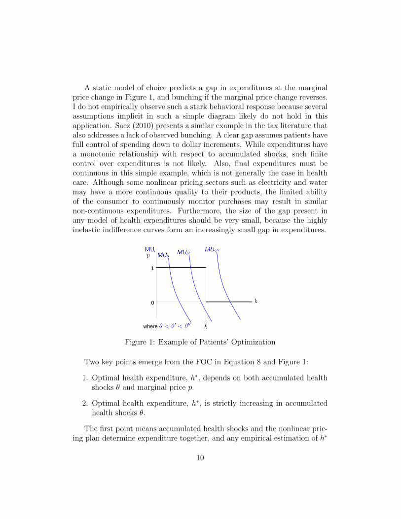
A static model of choice predicts a gap in expenditures at the marginalprice change in Figure 1, and bunching if the marginal price change reverses.I do not empirically observe such a stark behavioral response because severalassumptions implicit in such a simple diagram likely do not hold in thisapplication. Saez (2010) presents a similar example in the tax literature thatalso addresses a lack of observed bunching. A clear gap assumes patients havefull control of spending down to dollar increments. While expenditures havea monotonic relationship with respect to accumulated shocks, such finitecontrol over expenditures is not likely. Also, final expenditures must becontinuous in this simple example, which is not generally the case in healthcare. Although some nonlinear pricing sectors such as electricity and watermay have a more continuous quality to their products, the limited abilityof the consumer to continuously monitor purchases may result in similarnon-continuous expenditures. Furthermore, the size of the gap present inany model of health expenditures should be very small, because the highlyinelastic indifference curves form an increasingly small gap in expenditures.

where

1

0

,

Figure 1: Example of Patients’ Optimization

Two key points emerge from the FOC in Equation 8 and Figure 1:

1. Optimal health expenditure, h∗, depends on both accumulated healthshocks θ and marginal price p.

2. Optimal health expenditure, h∗, is strictly increasing in accumulatedhealth shocks θ.

The first point means accumulated health shocks and the nonlinear pric-ing plan determine expenditure together, and any empirical estimation of h∗

10

should flexibly incorporate both. Second, optimal health expenditure, h∗,strictly increases with higher accumulated health shocks, θ. This strictlymonotonic relationship reflects the balance between utility condition (5),complementarities between h and θ, and utility condition (2), decreasingmarginal utility of health expenditure.

The nonlinear pricing schedule’s presence in Point 1 makes elasticity esti-mation difficult for several reasons, however. The first source of bias is thathi and pi are simultaneously determined by the deductible level of expendi-ture, h̄. Additionally, the underlying unobserved θi determines both hi andpi. Higher levels of accumulated health shocks induce a higher hi and itscorresponding p. Fixing this simultaneous determination problem is nontriv-ial. Observable patient characteristics used to proxy for unobserved θi arelikely correlated with the error term. For example, the latent accumulatedhealth shocks related to an 80-year-old patient’s expenditures compared witha 20-year-old patient’s expenditures are correlated. This paper’s method willuse estimation that does not require an uncorrelated i.i.d. error term.

Previous health elasticity approaches use average expenditures of demo-graphically similar populations to control for illness severity (Cherkin et al.(1989), Scitovsky and Snyder (1972), Scitovsky and McCall (1977)). How-ever, the health shock θ distribution potentially changes between comparisonyears. For example, demand for physician services includes time-confoundingfactors such as differences in flu seasons or the availability of new treatmentsor drugs. More importantly, the most price-sensitive patients have the op-portunity to drop out of the sample through dis-enrollment as prices increase.This paper’s estimation method compares behaviors within a year, so it re-lies on within-period variation. This avoids the intertemporal problem of exitfrom and entry into the insurance plan.

Another approach to the endogeneity problem above is to use instru-mental variables for price, that are independent of a patient’s accumulatedhealth shocks. For example, as in Eichner (1998), Kowalski (2010), wherethe authors take advantage of when unexpected injuries push a family overthe deductible. This approach works well in a setting of general medicalexpenditures with family deductibles. Duarte (2012) broadens this instru-mental variables approach using a wider population in Chile, an importantcontribution of non-US elasticity estimation. The advantage of the approachpresented here is it can be used in a broad range of applications outside ofsuch an empirical setting where “unexpected injury” instruments may beharder to construct, such as nonlinear rate schedules in public utilities and

11

telecommunications, or prescription drugs. This approach can also be usedon individual coverage observations, as in this application, or in chronic dis-ease populations which lack an unexpected component.

The model of health expenditure choice above applies to a patient’s de-cision over a defined benefit period. Although a patient’s intertemporal de-cisions across or within benefit periods are interesting as well, the aboveframework is used for several reasons. First, the motivation for this methodis to inform policy on nonlinear pricing schedules, which generally apply toexpenditures over a pre-defined benefit period. Long-term elasticities area different policy question.4 Second, any effects on the estimates of a pa-tient’s ability to postpone treatment into the next benefit period dependson how much this delaying behavior varies across years in the populationas a whole. Postponing treatment until the following year is a concern inthis framework only if the extent of intertemporal substitution of the popu-lation changes yearly in a plan. This characteristic is unlikely to change inconsecutive years given local changes in the price schedule. If the ability topostpone health care is relatively constant from year to year, then this sim-ply represents another aspect of the underlying accumulated health shockdistribution. The broad health shock measure includes the time-sensitivityof care. Empirically, patients in the data display great persistence in healthcare spending year over year.

3. Estimation Method

The general model of health expenditures reveals two important deter-minants of health expenditures: marginal prices, pi, and accumulated healthshocks, θ. Marginal price data is generally easy to obtain. Data on accu-mulated health shocks is much more difficult, however. Besides the difficultyin obtaining identifiable data on diagnoses, constructing a health shock vari-able out of diagnoses is necessarily subject to ad hoc assumptions. Mostimportantly, any measure of accumulated health shocks will still have a largeobserved error component because of the endemic difficulty in measuringhealth.

In the model above, accumulated health shocks are essentially a latenterror term. The θ term is any unobserved health characteristic, and health

4Aron-Dine et al. (2012) address this understudied question nicely with a natural exper-iment revealing a patient’s intertemporal choices along a year when faced with a deductible.

12

expenditures are increasing in this unobserved, latent error term. Matzkin(2003) presents a framework to address this type of latent error nonpara-metrically. Identification using the Matzkin (2003) framework is off the factthat marginal price is constant within the estimation regions on each side ofthe nonlinearity, but the distribution of θ values change along the estimationwindow.5

This framework has several advantages in this setting. Nonparametricspecification allows the unobservable random term to be built into the esti-mator from within the model. The estimator is freed from the assumptionof additive error present in any OLS specification, allowing health statusto influence expenditures flexibly and nonlinearly. Nonparametric estima-tion also relaxes the OLS requirement that the error term has a mean zerodistribution.

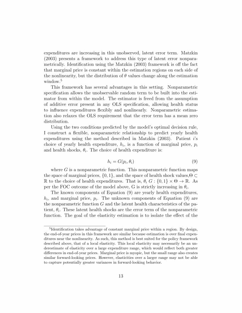
Using the two conditions predicted by the model’s optimal decision rule,I construct a flexible, nonparametric relationship to predict yearly healthexpenditures using the method described in Matzkin (2003). Patient i’schoice of yearly health expenditure, hi, is a function of marginal price, piand health shocks, θi. The choice of health expenditure is:

hi = G(pi, θi) (9)

where G is a nonparametric function. This nonparametric function mapsthe space of marginal prices, {0, 1}, and the space of health shock values,Θ ⊂R to the choice of health expenditures. That is, θi G : {0, 1} × Θ → R. Asper the FOC outcome of the model above, G is strictly increasing in θi.

The known components of Equation (9) are yearly health expenditures,hi, and marginal price, pi. The unknown components of Equation (9) arethe nonparametric function G and the latent health characteristics of the pa-tient, θi. These latent health shocks are the error term of the nonparametricfunction. The goal of the elasticity estimation is to isolate the effect of the

5Identification takes advantage of constant marginal price within a region. By design,the end-of-year prices in this framework are similar because estimation is over final expen-ditures near the nonlinearity. As such, this method is best suited for the policy frameworkdescribed above, that of a local elasticity. This local elasticity may necessarily be an un-derestimate of elasticity over a large expenditure range, which would reflect both greaterdifferences in end-of-year prices. Marginal price is myopic, but the small range also createssimilar forward-looking prices. However, elasticities over a larger range may not be ableto capture potentially greater variances in forward-looking behavior.

13

function G on the outcome of hi due solely to changing pi, while holding θiconstant.

Figure 2 displays the intuition behind the function G for the case of adeductible. Figure 2 represents a narrow expenditure region surrounding thedeductible. Consider first the left-hand Panel 2a. The horizontal axis isincreasing in the latent component, the health shocks θi, while the verticalaxis is increasing in health expenditure, hi, which is observed. Any line onthe figure shows how G maps an increase in the latent accumulated healthshocks, θi, to a corresponding increase in choice of health expenditure, hi, onthe vertical axis. The vertical dashed line at θ̄ denotes the location of thelevel of health shocks which leads to spending at the level of the deductible.Patients pay a marginal price of one before hitting the deductible, and afterthe deductible patients pay a marginal price of zero, labeled p = 1 and p = 0,respectively.

Panel 2a displays the first step of identifying G. When the p argument inEquation (9) is constant within each region, Matzkin (2003) shows that thefunction G can be identified within that region. The function hi = G(1, θi),shown by the solid line, can be estimated based on all the θi < θ̄ wherep = 1. Above θ̄, the function hi = G(0, θi), shown by the dashed line, canbe calculated based on all the θ > θ̄ where p = 0. These figures show G as alinear function for expositional purposes; final estimation is more flexible.

Note that the slope of the dashed line where p = 0 is more steep than thesolid line where marginal p = 1. This shows the same increase in accumulatedhealth shocks maps to a larger increase in health expenditures when priceis zero. To predict health expenditures in full out-of-pocket region on thediagram, choose a θ∗i and plug it into the estimated equation hi = G(1, θ∗i ).

Panel 2b shows the second step of the estimation – the prediction of healthexpenditures for different marginal prices. An elasticity calculation requires apatient’s health expenditure choice at two different prices, given a fixed levelof latent accumulated health shocks. To do this, use the slope of the functionG where p = 0, which is the dashed line hi = G(0, θi) in Panel 2a. Transferthis slope into the region where p = 1. Panel 2b demonstrates this wherethe dashed line with the steeper slope begins at the origin and rises abovethe solid line representing G when p = 1. To predict the choice of healthexpenditure given two different prices, the estimator isolates a given level ofhealth shocks, θ∗i , and uses the solid line hi = G(1, θ∗i ) and the dashed linehi = G(0, θ∗i ) to predict the choice of hi when p = 1 and p = 0, respectively.

The unknown in the diagrams described so far is the distribution of the

14

health

expenditure

(a) Step 1: Estimate G in each pricing region

health

expenditure

(b) Step 2: Predict h for fixed θ∗ using G

Figure 2: Simplified exposition of estimator

15

latent accumulated health shocks. If we knew the underlying distribution ofhealth shocks, we could use this to estimate the function G. Matzkin (2003)shows that latent θ can be proxied by the percentile function because thefunction G is strictly increasing in θi. That is, even without knowing theexact shape of Fθ distribution, if a particular patient’s health expendituresare in the 75th percentile of expenditures, then the latent health shocks ofthat patient are also in the 75th percentile of health shocks. The percentilefunction is bijective, surjective, and monotonically increasing. Let Fh be thedistribution of observed individual health expenditures, hi, and Fθ be thedistribution of the individual omitted characteristics θi. The shape of theunderlying distribution of omitted characteristics, Fθ, can be identified bymapping the percentiles of the health expenditure distribution, Fh. In thisway, the unknown θi can be inferred by the econometrician, and treated asdata.

Now that θi can be identified, we can estimate the function G from Equa-tion (9). In each region where marginal price is constant, this function mapsa change in accumulated health shocks, θi, to a choice of health expenditure,hi, given a fixed marginal price set by the price schedule.

Estimation uses a more flexible nonparametric approach than displayedin Figure 2. Local linear regression allows the functional form of G in eachmarginal price region to be flexible. Where θi < θ̄ – the left-hand side of thediscontinuity– the estimation equation is:

minaL,bL

∑θi<θ̄

K

(θi − θ0

κ

)(hi − aLθ0 − b

Lθ0

(θi − θ0))2

(10)

Analogously, where θi > θ̄, the right-hand side of the discontinuity– theestimation equation is:

minaR,bR

∑θi<θ̄

K

(θi − θ0

κ

)(hi − aRθ0 − b

Rθ0

(θi − θ0))2

(11)

where aLθ0 ,aRθ0

are constant coefficients and bLθ0 , bRθ0

are slope coefficientsbased around the value θ0, K is a kernel estimator with bandwidth k, andeach θ0 is in a series of points used by the local linear regression over the θrange of estimation.

Local linear regression uses Equations 10 and 11 to construct G(1, θ) andG(0, θ) over a window of observations on either side of the nonlinearity. The

16

estimation method combines Matzkin (2003) and intuition from a regressiondiscontinuity design approach. The function G(1, θ) measures the rate ofchange in health expenditures as θ increases, for a fixed marginal price of1. The function G(0, θ) measures the rate of change in expenditures as θincreases, for a fixed marginal price of 0. As these two functions approachthe nonlinearity, the limit latent θ value is the same, yet the marginal pricecomponent of the functions G is constant. The method compares the differ-ence in the slopes of G as they approach the limit. The estimator controlsfor the price schedule’s simultaneity between price and quantity by isolatingthe changing θ values in the constant marginal price region.

The estimator is essentially measuring the change in the slope of a cu-mulative distribution function at the point of the nonlinearity. Unobservedheterogeneity, θ, changes over the entire estimation window, so the estimatorrecovers behavioral responses using a nonparametric inverse cdf identified viathe Matzkin (2003) framework. The function G is similar to a cdf because theunobserved accumulated health shocks can be proxied with a percentile func-tion. Identification occurs through the changes in the slope in each region,where price is fixed, but the cdf relationship is flexible. Cdf interpretationrearranges Figure 2 so that the horizontal axis would be spending and thevertical axis would be percentiles of spending. The slope of G measures thepercentiles of spending for a given level of expenditure. The change in slopesimply measures how a small change in θ leads to a change in the probabilitythat the corresponding hi is a large jump in cumulative probability.

Though borrowing intuition from a regression discontinuity design, oneimportant difference between this approach and RD design is that here thepatient’s omitted characteristics are the forcing variable that determines apatient’s marginal price. Because the choice of hi is strictly monotone in theomitted characteristics θi, the patient’s level of θi is what forces him to theleft or to the right of the discontinuity. Identification in this method is notthe same as a regression discontinuity design, which requires omitted char-acteristics to be the same in each region. This method specifically does notrequire this assumption. Here, G nonparametrically incorporates changesunobserved characteristics, and instead identification uses the difference therelationship generated by the unobserved characteristics, G, between con-stant marginal price regimes.

The final formula for calculating elasticity uses the local linear regressionslope coefficients at the limit because we are interested in the point where pa-tients’ omitted θ are the most similar. The local linear regressions Equations

17

11 and 10 from above are rearranged to replicate Panel 2b as follows:First write hi for the observations θi < θ̄ at the threshold limit θ = θ̄

hi|(θi < θ̄) = aLθ̄ + bLθ̄ (θi − θ̄)= aLθ̄ − b

Lθ̄ θ̄ + bLθ̄ θi

= AL + bLθ̄ θi (12)

hi|(θi > θ̄) = aRθ̄ + bRθ̄ (θi − θ̄)= aRθ̄ − b

Rθ̄ θ̄ + bRθ̄ θi

= AR + bRθ̄ θi (13)

where aLθ̄, aR

θ̄, bL

θ̄, and bR

θ̄are the constants and slope coefficients at the

limit θ̄.6

To replicate Figure 2, write a general equation for hi starting at the leftregion intercept, AL, by using an indicator function equal to one when p = 1:

hi = AL + bRθ̄ θi + (bLθ̄ − bRθ̄ ) θi 1{p = 1} (14)

Equation 14’s slope coefficient order, (bLθ̄− bR

θ̄), is for the deductible case,

where the p = 0 region is the right-hand side. Equation 14 solved for hi(p =1) and hi(p = 0):

hi(p = 1, θi) = ALθ̄ + bLθ̄ θi (15)

hi(p = 0, θi) = ALθ̄ + bRθ̄ θi (16)

In this application, I use percentage change elasticity. This is to accountfor the fact that enrollees are moving from a no coverage region into a fullcoverage region.7 Elasticity, η, of moving from full out-of-pocket into fullcoverage is:

6Refer to the appendix for a construction of the estimator using the parametric formof the general utility model. In this case, the coefficients can be built out of structuralparameters.

7Given the extreme change in marginal price, percentage change is more informativethan a midpoint elasticity, although other applications with smaller price changes couldcertainly use Equation 14 in midpoint formula if so desired. Aron-Dine et al. (2013) use amidpoint formula, for example.

18

η =%∆hi%∆p

=

[hi(p = 0, θi)− hi(p = 1, θi)

hi(p = 1, θi)

]/

[0− 1

1

]=−[ALθ̄

+ bLθ̄θi − (AL

θ̄+ bR

θ̄θi)]

ALθ̄

+ bRθ̄θi

=−(bR

θ̄− bL

θ̄) θi

ALθ̄

+ bRθ̄θi

(17)

Which evaluated at θ̄ is equal to:

η = −(bRθ̄ − bLθ̄ )θ̄

h̄(18)

The case of a Health Savings Account (HSA), where patients face oppositemarginal prices, reverses the order of bL and bR slope coefficients.

4. Data

4.1. Data

The dataset is proprietary claims-level data for an employer with severallocations. The employer is self-insured and all individual claims are reportedfor each of the three years 2002, 2004, and 2005.8 Each claim entry con-tains all information necessary for classifying the services received and toremit payments. Each claim has information on the costs incurred by thepatient and the amount covered by the employer, as well as information onthe treatment facilities, procedure codes, and diagnoses. An advantage of aself-insured employer is that income information is available to identify thesocioeconomic status of the population.

In particular, I study the Consumer-Driven Health Plan (CDHP) optionavailable to enrollees, which is a high-deductible plan. Enrollees had theoption to enroll in four other plans offered by the employer. The effect thismay have on estimates comes through in the broader generalizability of the

8In the years 2002-2005, missing enrollee assignment codes in 2003 prevented using thisyear in estimation.

19

type of enrollees who chose this plan, but not in the estimates within theplan. I show that this estimation method is not subject to selection biasfor within-plan estimates. Characteristics of patients enrolled in this plandetermines the broader applicability of these elasticity estimates.

The CDHP plan contains two nonlinearities. The first nonlinearity re-sults from an employer-funded Health Savings Account (HSA), where theemployer deposits funds that can be used to purchase health care from thefirst dollar spent until the patient exhausts the HSA. The second nonlinearityis a deductible. Figure 3 illustrates the nonlinear structure of this plan.

health

expenditure ($)

patient out-of-

pocket cost ($)

full

coverage

HSA 0

full

out-of-pocket

full

coverage

deductible

full

out-of-pocket

full

coverage

(a) CDHP in levels

health

expenditure ($)

patient marginal

price ($)

full

coverage

HSA 0

full

out-of-pocket

full

coverage

deductible

1

(b) CDHP in marginal cost

Figure 3: Nonlinear Pricing Schedule, Consumer Driven Health Plan

The threshold levels of both the HSA and the deductible change fromyear to year. This variation in nonlinearity thresholds helps identify patients’responses to the nonlinear pricing schedules in two ways. If the nonlinearitychanges each year, this lends robustness to the estimation method if estimatesremain similar over years. Second, the estimator has strong validity forobservations just at the nonlinearity, but validity is limited for observationsfar from the nonlinearity. However, with estimates at proximate intervals,elasticity is estimated over an expanded range of expenditures. Table 1 listsplan nonlinearities during the years 2002, 2004, and 2005.

Table 2 reports plan summary statistics for patients who enrolled undersingle coverage for the entire 12-month benefit period. The first rows reportthe yearly means and medians of total expenditure, employer cost, the yearlymeans of the amount of HSA used, and the amount of deductible fulfilled.Average total expenditure for all three years was $7,387. However, health

20

Table 1: Consumer Driven Health Plan (CDHP) structure

First nonlinearity Second nonlinearityYear HSA Deductible2002 $500 $1,2502004 $750 $1,5002005 $600 $1,500

expenditure distributions tend to be skewed, so median total expenditurewas lower in all years. Lower expenditure levels of employer cost comparedto total expenditures reflect positive out-of-pocket costs to patients. Patientexpenditure variables in Table 2 include the amount of the deductible ful-filled and the amount of the HSA used. An average patient’s total incurredspending towards his deductible was $644. The average amount used of theHSA on incurred spending was $319.9

Patient-level characteristics for single-coverage, full-year enrollees in theinsurance plan are reported in the bottom rows of Table 2. Plan enrollmentin this category grew from 165 enrollees in 2002 to 349 in 2005. The averageage over all three years is 48, and the average salary for the enrollees is$55,934. The plan enrolled 72 percent women.

5. Elasticity Estimation Results

I estimate elasticities over patients’ yearly expenditures within the esti-mation windows for each of the three years. Yearly estimates are necessarybecause the level of the nonlinearities, and thus the threshold θ̄, changes ev-ery year. Table 3 displays the results for the first plan nonlinearity, the HSA.Table 4 displays results for the second nonlinearity, the deductible. I calcu-late standard errors using the asymptotic distribution properties developedin Bajari et al. (2010).10

9The first year this plan was available was 2002, which explains the lower enrollmentstatistics and associated spending levels. An advantage of several years is that resultscan be compared across several years if there is concern that the first year was differentbecause of its novelty.

10In this method, the difference between the true limit of the expenditure choices and theestimated value of this limit from above and below converges to an independent exponentialvariable with hazard rates of f−(hL) from below and f+(hR) from above. The local linear

21

Table 2: Data Summary for Full Sample

Year 2002 2004 2005 OverallAverage Expenditures

Total Expenditure $5,251 $7,130 $8,647 $7,387(median) $1,492 $2,024 $2,288 $2,016

Employer Cost $4,852 $6,560 $7,824 $6,746(median) $990 $1,551 $1,899 $1,537

Deductible Used $540 $665 $672 $644HSA Used $257 $377 $292 $319

DemographicsEnrollees 165 341 349 855Percent Female 71 72 72 72Age 46 48 48 48Salary $58,783 $51,224 $58,965 $55,935Single coverage 100% 100% 100% 100%

Includes only single coverage, full year enrollment.

The heading of Table 3 reports the elasticity formula from Equation 18,arranged for the HSA nonlinearity. The first column of Table 3 reportsthe year, and the second column is the number of observations within theestimation window around the HSA. The third column reports the level ofthe HSA in that year. The final column reports elasticity estimates.

The elasticity estimates around the HSA nonlinearity are -0.25 in 2005,-0.26 in 2004, and -0.33 in 2002. All are inelastic. The similarity acrossyears is noteworthy because the nonlinearity value of h̄ changes across yearsbetween $500 and $750. The estimates reported in this paper are for a$300 window and based on an Epanechnikov kernel, but are robust to other

regression slopes bLθ̄

and bRθ̄

are then the inverse of these hazard rates, respectively. Thehazard rates are estimated from the data with a one-sided kernel density. The differencebetween the estimated and true value of the difference in the slopes, (bL

θ̄− bR

θ̄), converges

asymptotically to a normal distribution with variance calculated using f−(hL), f+(hR),and properties of the chosen kernel.

22

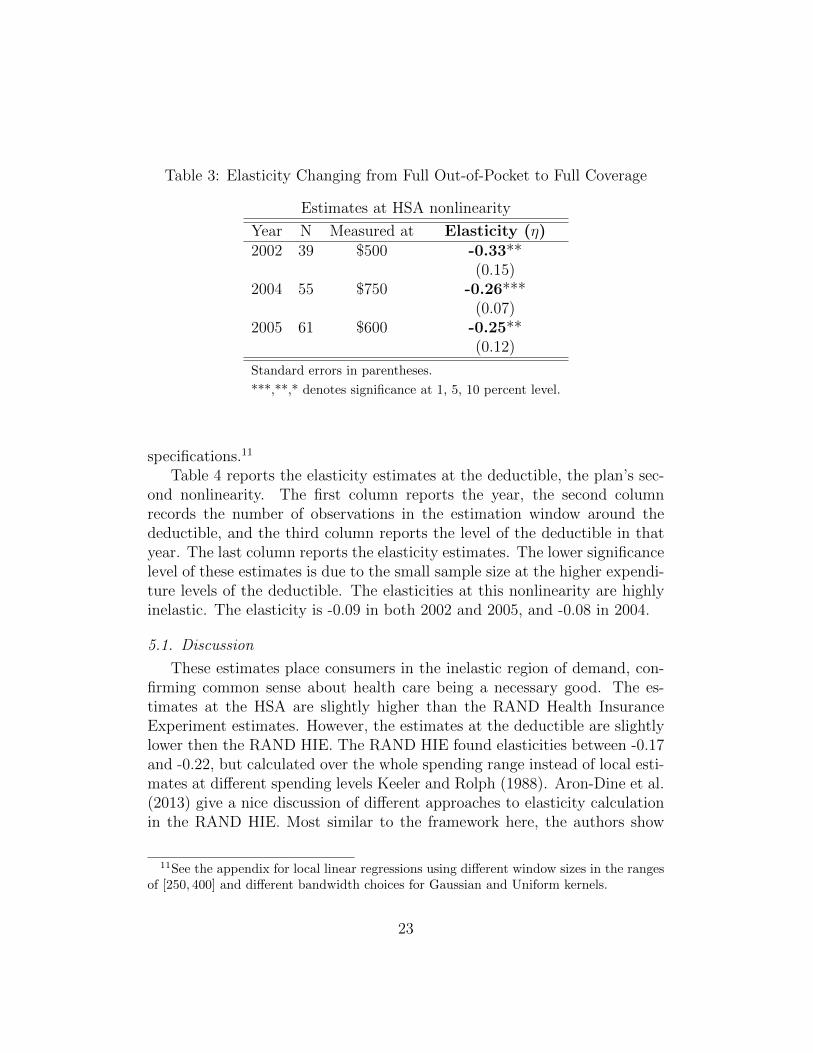
Table 3: Elasticity Changing from Full Out-of-Pocket to Full Coverage

Estimates at HSA nonlinearity

Year N Measured at Elasticity (η)2002 39 $500 -0.33**

(0.15)2004 55 $750 -0.26***

(0.07)2005 61 $600 -0.25**

(0.12)

Standard errors in parentheses.

***,**,* denotes significance at 1, 5, 10 percent level.

specifications.11

Table 4 reports the elasticity estimates at the deductible, the plan’s sec-ond nonlinearity. The first column reports the year, the second columnrecords the number of observations in the estimation window around thedeductible, and the third column reports the level of the deductible in thatyear. The last column reports the elasticity estimates. The lower significancelevel of these estimates is due to the small sample size at the higher expendi-ture levels of the deductible. The elasticities at this nonlinearity are highlyinelastic. The elasticity is -0.09 in both 2002 and 2005, and -0.08 in 2004.

5.1. Discussion

These estimates place consumers in the inelastic region of demand, con-firming common sense about health care being a necessary good. The es-timates at the HSA are slightly higher than the RAND Health InsuranceExperiment estimates. However, the estimates at the deductible are slightlylower then the RAND HIE. The RAND HIE found elasticities between -0.17and -0.22, but calculated over the whole spending range instead of local esti-mates at different spending levels Keeler and Rolph (1988). Aron-Dine et al.(2013) give a nice discussion of different approaches to elasticity calculationin the RAND HIE. Most similar to the framework here, the authors show

11See the appendix for local linear regressions using different window sizes in the rangesof [250, 400] and different bandwidth choices for Gaussian and Uniform kernels.

23

Table 4: Elasticity Changing from Full Out-of-Pocket to Full Coverage

Estimates at Deductible nonlinearity

Year N Measured at Elasticity (η)2002 22 $1250 -0.09

(0.17)2004 40 $1500 -0.08*

(0.05)2005 34 $1500 -0.09

(0.06)

Standard errors in parentheses.

***,**,* denotes significance at 1, 5, 10 percent level.

that HIE participants switching from free care to a 95% coinsurance hadan elasticity of approximately -0.23. The advantage of this approach’s localestimation is it sidesteps the limitations of calculating a single price for acomplex range of expenditures and nonlinearities in plans.

Given the deductible framework in this paper, the most appropriate lit-erature comparisons are those examining the changes from full insurance tonone, or vice versa. Boes and Gerfin (2013) compare a managed care planwith temporary full insurance against recently introduced cost-sharing mea-sures. The authors also find elasticity decreasing for higher levels of healthexpenditures, with an average elasticity of -0.148, after adjusting for selectionout of the HMO.

Outside of the RAND HIE, previous literature estimates elasticities fora range of types of health expenditures. Among the estimates that applyspecifically to general medical expenditures, Cherkin et al. (1989) found pri-mary care physician visits responded the most to the introduction of a $5copay. Visits decreased by approximately -10% for what was approximately15% of a typical visit charge. This response may be slightly larger than theestimates in my data, but the Cherkin et. al data came from an HMO whereprimary care physician’s roles as gatekeepers imply a higher time cost pervisit as a baseline comparison. Selby et al. (1996) found a -14% decline inemergency room visits from a much larger copay introduction of $25-$35.The elasticity implied by these numbers is slightly less responsive than thosepresented above, which follows from emergency room visit versus physician

24

visits.Claims-level data allows us to look more closely into why these local

elasticities are different at different points of the spending distribution. Es-timates are more inelastic at the higher deductible nonlinearity comparedwith the HSA nonlinearity. The first explanation for this may be because ahigher level of expenditures means a higher level of illness severity, which isassociated with less price sensitivity. To examine this hypothesis, Tables 5and 6 compare facility types and services in the HSA local estimation windowversus the deductible local estimation window.

Table 5 shows the percentage of expenditures within the local estimationwindow for a given facility type, comparing the HSA and deductible estima-tion windows. For both windows, physician offices are the largest categoryof spending. However, physician offices are a much higher percentage of ex-penditures in the HSA window, at 70 percent compared to only 58 percentaround the deductible. More claims in the deductible take place at moreintensive facilities compared to the physician office. Hospital Outpatient fa-cility use is one of the more striking differences between the two estimationsamples. Hospital Outpatient facilities were 8 percent of expenditures in thedeductible, which is double the percent found in the HSA sample. This in-dicates the higher deductible spending levels are correlated with more severehealth shocks, which leads to lower price sensitivity.

The services reported by patients’ claims also suggest increasing severitytoward the deductible, as well as an indication that spending may be less dis-cretionary and more lumpy as the mix of services changes between the HSAregion and the deductible region. Table 6 reports the percentage of expen-ditures in the top 5 services in the estimation windows. The two estimationwindows both show significant spending in Lab/Pathology, X-Ray Diagnos-tics, and Vision services. However, the HSA region shows a combined totalof 32% spending on Physician Care and Routine Physical services, neitherof which make the top five at the deductible estimation window. Patientshave a greater ability to control the amount of Routine Physical services, indeciding to complete an annual physical or not. In contrast, the deductibleregion begins to have more Surgery services (5 percent), which is a servicethat may be less discretionary than Routine Physical.

The broader application of these elasticities depends on the sample popu-lation and its generalizability to a larger population. This method’s estimateshave a high level of internal validity within the sample population, but theexternal validity of these estimates to populations outside the sample re-

25

Table 5: Facility Type Comparison: HSA vs. Deductible

Percent Facility Type ExpendituresHSA

70% Physician’s Office $66,1376% Independent Lab $5,7625% OB/GYN Office $4,5494% Hospital Outpatient $4,055

Deductible58% Physician’s Office $79,3129% Independent Lab $12,6148% Hospital Outpatient $10,8815% Clinic $6,154

Expenditures are total within the local estimation window

Windows are within a $300 window on each side of the nonlinearity

Table 6: Type of Service Comparison: HSA vs. Deductible

Percent Service Type ExpendituresHSA

22% Physician Care $20,51819% Lab/Pathology $17,53613% Vision $12,39812% X-Ray Diagnostic $11,25210% Routine Physical $9,710

Deductible19% Lab/Pathology $25,90213% X-Ray Diagnostic $18,4028% Psychotherapy $11,3776% Vision $8,8495% Surgery $7,494

Expenditures are total within the local estimation window

Windows are within a $300 window on each side of the nonlinearity

26

quires further discussion. There are two points of general applicability ofthis sample population. First, the spending levels are typical of the medianspending of a privately insured individual under 65 during the time period.U.S. median health expenditure was $1,032 in 2005 (AHRQ (2005)), whichlies between the expenditure levels of the HSA estimates ($500 - $750) andthe deductible estimates ($1250-$1500). Comparing these estimates to pre-vious work also should be restricted to the mix of services found in theseHSA and deductible ranges. Secondly, the insurance is employer-sponsored,which is the most common type in the U.S.

There are a few ways in which this population may not translate to a moregeneral U.S. health care population. The patients in this sample are richerthan the average U.S. population, thus elasticity for a general populationmay be lower if income effects hold. Additionally, the patients in the samplepopulation are, on average, healthier than the firm’s population as a whole.12

If the severity of health shocks is lower than a more general privately-insuredpopulation, these elasticity estimates may show patients to be more respon-sive to marginal prices if elasticity decreases with the severity of a healthshock. Finally, willingness to participate in a high-deductible plan couldhave implications for the risk-aversion parameters of patients. In a studyon individuals in private insurance, van de Ven and van Praag (1981) findthat increasing income and education correlate positively with demand for adeductible.13 Given these caveats, these estimates are most useful as a localelasticity, but are not atypical of expenditures in U.S. employer-sponsoredplans.

12This data is similar to the national statistics on enrollees in Consumer Driven HealthPlans. Enrollees in CDHPs tend to be richer, more educated, and healthier than theircounterparts in other employer-sponsored plans Kaiser Family Foundation (2006). TheKaiser Family Foundation’s 2006 Survey of CDHP enrollees found that 45 percent ofCDHPs enrollees had salaries over 75,000, compared with 30 percent of the control groupof employer-sponsored enrollees in other plans. 64 percent of CDHP enrollees reportedbeing in excellent or very good health, compared with 52 percent in the control group.

13Einav et al. (2012) develop a model where patients select an insurance plan basedon both aggregate risk and the “slope” of the pricing structure. This suggests that theremay be selection into high-deductible plans based on the pricing schedule in addition toexpected total out-of-pocket costs. Given this model, the patients selected into a CDHPplan may be less price-responsive than a general population. This could bias my finalestimates downward compared with a general population.

27

5.2. Robustness

The identifying assumption in the estimation method is that the latenterror term, θ, is continuous across the nonlinearity but the price changes.In this application, the latent error is accumulated health shocks over theyear of the insurance pricing structure. The θ term should be capturingdifferences in these accumulated health shocks within a $300 window on eachside of the spending level of each nonlinearity, but of which are below $2,000.The resulting elasticity can be interpreted as a local interaction of healthshocks and the pricing structure. Although claims-level detail is not strictlynecessary to implement the estimation method, we can use detail on patientclaims to verify that these estimates are capturing reactions to accumulatedhealth shocks within a narrow window of final expenditures, and not fixedcharacteristics such as age and gender.

As discussed in the estimation section, the accumulated health shocksθ are the forcing variable into pre- or post-nonlinearity region. Since ageand gender are not health shocks within a $400 window, but instead a fixedendowment, Tables 7 and 8 test if there is selection on age and gender oneither side of the nonlinearity.14

Table 7 shows the results of both a means test and K-S test for differencesin the distribution of ages and gender on each side of the HSA estimationsample. None of the tests can reject the hypothesis that distributions of ageand gender are the same on each side of the nonlinearity. For each year, Iuse a means test to compare the average ages of sample individuals that fallpre-HSA versus post-HSA. Besides just the mean, I also run a K-S test ofequality of distributions comparing the age distribution just before versusjust after the HSA nonlinearity. Both the means test and the K-S testscannot reject equality of the age distribution in the pre versus post HSAsamples, up to a 15 percent confidence level. The bottom half of Table 7performs the same tests on the gender ratios and cannot reject equality forat least the 15 percent level for 2004 and 2005, and at least the 10 percentlevel for 2002.

Table 8 tests for equality of distributions in age and gender at the highernonlinearity threshold of the deductible. Neither the means tests or the K-

14Age and gender likely enter the patient’s problem in the initial choice of plan, as afixed health status level. In the estimation window, the change in the θ variable maps toa forcing variable within a narrow window of expenditures– the patient’s age and genderwould enter as a fixed effect.

28

Table 7: Testing for Differences in Age and Gender in Estimation Sample:Before vs. After HSA

Year N Means test K-S Test ResultAge

2002 39 t = −1.60 D = 0.31 Cannot Reject*(p = 0.12) (p = 0.25)

2004 55 t = −1.20 D = 0.20 Cannot Reject*(p = 0.23) (p = 0.54)

2005 61 t = 0.17 D = 0.21 Cannot Reject*(p = 0.87) (p = 0.45)

Gender2002 39 t = 1.51 D = 0.24 Cannot Reject**

(p = 0.14) (p = 0.54)2004 55 t = 0.08 D = 0.01 Cannot Reject*

(p = 0.23) (p = 1.00)2005 61 t = −0.07 D = 0.01 Cannot Reject*

(p = 0.95) (p = 1.00)

T-statistics for means tests between before and after HSA nonlinearity.

D-statistics for Kolmogorov-Smirnov test of distributional equivalence.

P-values in parentheses under the respective statistics.

*, ** – Test is not significant at the 15 percent level or below, 10 percent or below.

29

S test for equality of age can be rejected for 2002-2005, for at least a 15percent confidence level. The only test to come close to showing significantdifferences pre deductible and post deductible is the means test on genderfor 2005, which still is not significant at the 5 percent level.

Table 8: Testing for Differences in Age and Gender in Estimation Sample:Before vs. After Deductible

Year N Means test K-S Test ResultAge

2002 22 t = 0.12 D = 0.23 Cannot Reject*(p = 0.91) (p = 0.95)

2004 40 t = −0.36 D = 0.20 Cannot Reject*(p = 0.23) (p = 0.76)

2005 34 t = −0.67 D = 0.33 Cannot Reject*(p = 0.51) (p = 0.21)

Gender2002 22 t = −0.91 D = 0.21 Cannot Reject*

(p = 0.37) (p = 0.98)2004 40 t = −0.36 D = 0.05 Cannot Reject*

(p = 0.72) (p = 1.00)2005 34 t = −1.85* D = 0.26 Cannot Reject***

(p = 0.07) (p = 0.49)

T-statistics for means tests between before and after HSA nonlinearity.

D-statistics for Kolmogorov-Smirnov test of distributional equivalence.

P-values in parentheses under the respective statistics.

*, *** – Test is not significant at the 15 percent level or below, 5 percent or below.

One possibility for why a patient crossed over the threshold that is notconsistent with the model above is that final claims were for a more ex-pensive doctor, which would mean that elasticity estimates were capturing ageographic effect, not a response to health shocks. Therefore, another robust-ness check compares the location of services before and after the nonlinearity.As such, Table 9 compares service zipcodes on each side of the HSA limitin the estimation sample for the two years when zipcode information wasavailable. In 2004, the top three zipcodes were identical on each side of thenonlinearity. In 2005, two of the top three zipcodes were the same. The

30

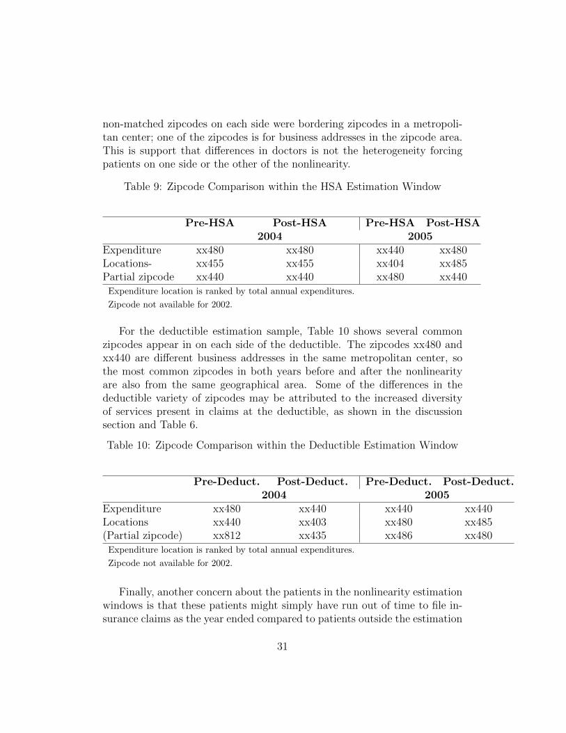
non-matched zipcodes on each side were bordering zipcodes in a metropoli-tan center; one of the zipcodes is for business addresses in the zipcode area.This is support that differences in doctors is not the heterogeneity forcingpatients on one side or the other of the nonlinearity.

Table 9: Zipcode Comparison within the HSA Estimation Window

Pre-HSA Post-HSA Pre-HSA Post-HSA2004 2005

Expenditure xx480 xx480 xx440 xx480Locations- xx455 xx455 xx404 xx485Partial zipcode xx440 xx440 xx480 xx440

Expenditure location is ranked by total annual expenditures.

Zipcode not available for 2002.

For the deductible estimation sample, Table 10 shows several commonzipcodes appear in on each side of the deductible. The zipcodes xx480 andxx440 are different business addresses in the same metropolitan center, sothe most common zipcodes in both years before and after the nonlinearityare also from the same geographical area. Some of the differences in thedeductible variety of zipcodes may be attributed to the increased diversityof services present in claims at the deductible, as shown in the discussionsection and Table 6.

Table 10: Zipcode Comparison within the Deductible Estimation Window

Pre-Deduct. Post-Deduct. Pre-Deduct. Post-Deduct.2004 2005

Expenditure xx480 xx440 xx440 xx440Locations xx440 xx403 xx480 xx485(Partial zipcode) xx812 xx435 xx486 xx480

Expenditure location is ranked by total annual expenditures.

Zipcode not available for 2002.

Finally, another concern about the patients in the nonlinearity estimationwindows is that these patients might simply have run out of time to file in-surance claims as the year ended compared to patients outside the estimation

31

window. However, although December is the most common month of lastclaim both in and out of the estimation sample, less than 40 percent of thepatients in the estimation sample filed their last claim in December. Therewas a positive number of patients in the sample showing a last claim in everymonth of the year, with increasing probability of a last claim as the yearprogressed. This pattern is consistent with the larger population’s month oflast claim data.15

6. Moral Hazard Estimation

6.1. Setup

Plans with high reimbursement rates are often cited as inducing over-consumption and moral hazard because the patient bears very little of thecost of his health care. This refers to ex-post moral hazard, where patientsconsume more health care because insurance insulates them from its cost.Demand elasticities are often used as a proxy for ex post moral hazard. Itake this further by measuring the welfare impact between observed expendi-tures in my generous plan with predicted patient expenditures faced with fullout-of-pocket costs. Elasticity measures reveal patients’ responses to price.This counterfactual gets closer to what policy makers are really interestedin, which is the deadweight loss of insurance-induced demand changes.

To measure the amount of deadweight loss,the extent of moral hazard,I compare patient choice in two scenarios. The first scenario is a generousinsurance plan, which covers 100 percent of care. In the second scenario, allcare is paid for out-of-pocket for the same range of expenditures.16 Figure 4illustrates the basic concept behind the deadweight loss calculation. Whenthe consumer is fully insured and pays zero percent of his out-of-pocket costs,the consumer’s choice of health care, hi1, gives him consumer surplus ofA + B + C. The insurance company pays for the entire cost of this choiceof health care, which amounts to B + C + D. Net welfare in the free carescenario is (A−D). I predict the consumer’s choice, hi2, if paying 100 percent

15See Appendix for a histogram of month of last claim for each population.16In these scenarios, I use only changes in coinsurance. Although premiums are also

part of an insurance plan, choosing the changes in premiums between the two scenarioswould require several other assumptions on patient responses and how actuarially fair theinsurance plan is. The two scenarios going from full coverage to no coverage with nochange in premiums create an upper bound on the amount of moral hazard.

32

of the cost, with consumer surplus equal to A+B. In this second scenario thecost of care is the area B. Net welfare in the full out-of-pocket scenario is A.Thus, the area D is the amount of deadweight loss. To get a measure of thedeadweight loss D, I take the change in expenditure between full insuranceand full out-of-pocket, C+D, and subtract out the transfer the patient wouldneed to compensate him for the loss of C in the full out-of-pocket scenario.

OOP

price

Health Expenditures

A

D B C

MB

MC

Figure 4: Patient Choice and Welfare in Counterfactual

For empirical estimation of the reduction in health expenditure choice, Ilink each value of the estimated θi to observed full coverage health expendi-ture, hi1. I then use the slope coefficients estimated in Section 5 to predictthe counterfactual spending of each patient given full out-of-pocket payment,hi2. I use only those patients from the original HSA estimation window forthe moral hazard calculation, and I assume a constant elasticity around thenonlinearity. This HSA window is the most reasonable for calculations ab-stracting from income effects.

To calculate the compensating transfer for each patient, I use the followingutility function for the choice of health expenditure. Utility is based onthe conditions set on the general utility function in Section 2, where thepreference parameters satisfy ρ ε (0, 1) and γ > 0:

Ui(hi, θi, ci) = θihρi + (1− θi)ci − γ hi (19)

The parameters θi, hi, and c have the same interpretation as in the gen-eral mode. The γ parameter captures nonmonetary costs of health care, suchas time, and satisfies Condition (2) of the utility conditions in Section 2. The

33

utility function is decreasing in illness as long as hρi < ci.17 Utility is increas-

ing in health care expenditures up to marginal utility of zero, and marginalutility is decreasing in additional health expenditures. The final Condition(5) of the Utility Conditions holds that health care increases utility by agreater amount at higher levels of illness. I use individual salary informationfor non-health composite good consumption.

The two remaining unknowns in the utility function are: the risk-aversionparameter on health care expenditures, ρ, and the nonmonetary cost of healthcare, γ. I estimate these parameters from the data using a general methodof moments approach which chooses parameters which minimize the differ-ence between observed utility values and the predicted utility value in thecounterfactual. The estimated values for ρ̂ were approximately 0.23 and forγ̂ were approximately 0.31.18.

The compensating transfer C between the two scenarios is the amountof additional non-health care income the patient needs to remain indifferentbetween his utility consuming hi1 and his utility consuming only the lowerhi2. The transfer C enters the utility function as additional income in the fullout-of-pocket cost scenario. I set the two scenarios’ utility functions equal toeach other, and solve for C. The compensating transfer is then a function ofknown variables: estimated θi, ρ̂, and γ̂, observed hi1, and predicted hi2.

Ci(hi1, hi2, θi, ρ̂, γ̂) =θi

(1− θi)

(hρ̂i1 − h

ρ̂i2

)− γ̂

(1− θi)(hi1 − hi2) (20)

The compensating transfer is decreasing in ρ̂. This means that the sizeof the compensating transfer decreases as a patient becomes less risk adversein health care expenditures. The compensating transfer is also decreasing inγ̂, indicating that the amount of compensation for lost health care decreasesas the nonmonetary costs of the foregone care increase.

6.2. Moral Hazard Estimation Results

The measure of deadweight loss of moral hazard here is an upper bound,because it compares full coverage with no coverage. The deadweight loss is

17This condition always holds in my data, because ci is the salary left after health careexpenses, expenditure is less than $1,000 in the window, and ρ < 1.

18See the Appendix for further discussion of the GMM and tables of the utility parameterestimates

34

the portion of the difference in health expenditures where the marginal costis greater than the patient’s marginal utility – the part of the change thatthe patient does not require back in compensating transfer.19 Table 11 dis-plays the empirical results of the counterfactual in levels. The magnitude ofdeadweight loss is highest in 2004, which corresponds to the highest spendingwindow. The HSA cutoff was $750 in 2004 versus $600 and $500 in the otheryears. The median level of deadweight loss was approximately $66 in 2002,$134 in 2004, and $26 in 2005.

Table 11: Deadweight Loss Magnitude

Year p25 p50 p75

Level ($)

2002 9.65 66.26 144.942004 46.88 133.88 185.972005 9.63 25.88 64.38

Percent of Spending (%)

2002 4.75 20.29 31.682004 9.16 21.64 27.192005 2.68 6.59 12.65

To put the magnitude of the deadweight loss in context, Table 11 alsoreports the deadweight loss as a percentage of each patient’s free-care levelof spending. The median percentage of free-care spending level was approx-imately 20% in both 2002 and 2004. The median percentage was lower in2004, at approximately 7%. Patients at the beginning of the estimationwindow had the smallest change in spending, and thus the lowest levels ofdeadweight loss. The 25th percentile for deadweight loss as a percentage ofspending was 2.68% in 2005, 4.75% in 2002, and 9.16% in 2004. The upper

19The deadweight loss in the moral hazard calculation uses the observed charge to theinsurer as marginal cost. It is likely that the observed charge to the insurer is different thanthe true cost of providing the care. This true cost is often difficult to observe even withmore detailed provider-level data. If the insurer is making a profit margin above marginalcost on the amount listed in the claims data, then the deadweight loss measure will be anupper bound on moral hazard measured as marginal benefit greater than marginal cost.

35

end of the distribution was deadweight loss at a value of approximately 30%of free-care spending in 2002 and 2004. The 75th percentile in 2005 was12.65%.

Previous estimates of moral hazard in health expenditures have focusedon pure coinsurance elasticities. (See Newhouse (1993), Scitovsky and Sny-der (1972), Phelps and Newhouse (1974), Cherkin et al. (1989), Huang andRosett (1973)) This measure of moral hazard is more nuanced than an elas-ticity it takes into account the marginal value of health expenditures theconsumer gains, so not all increases in expenditure are moral hazard. Tocompare this counterfactual deadweight loss to previous estimates, we ex-pect pure elasticity measures of moral hazard be larger than this deadweightloss from generous insurance.

Existing estimates on changing from full insurance to no insurance havebeen measured both in natural experiments and the RAND Health Insur-ance Experiment (HIE). Scitovsky and Snyder (1972) used an exogenouschange in the coinsurance rate from free care to approximately 25 percentcoinsurance to find that health expenditures decreased by approximately 25percent. Similarly, Scheffler (1984) used a pre-post design on the introduc-tion of 40 percent coinsurance to outpatient care and found that expendituresdecreased by approximately 38 percent. Both of these percent decreases areclose to the deadweight loss percentages presented above. Assuming similarpatient populations, my estimates should be smaller than the previous stud-ies without marginal utility adjustment. However, my counterfactual alsomeasures a larger price change – going from full insurance to zero insurance.The RAND HIE is a closer match. Keeler and Rolph (1988) found that carealmost doubled going from no insurance to full insurance in the RAND HIE.To compare the HIE findings to the deadweight loss above, the HIE foundthat original expenditures decreased by half when patients had to pay fullout-of-pocket costs, and the median deadweight loss of my estimates is 20percent of original expenditures. This implies that less than half of the HIE’schange in expenditures was inefficient moral hazard.

The deadweight loss estimates above are of interest to policy makersconcerned with the transition from first-dollar coverage plans to higher out-of-pocket costs for patients. The results above suggest the upper bound onmoral hazard savings are, on average, 20 percent. These results apply to apopulation of group-insurance patients with relatively low levels of spending.The results also suggest that the introduction of these high deductible planshad welfare-improving effect for this population in the lower regions of patient

36

spending, though savings seemed to top off at less than approximately 30percent of existing spending.

7. Conclusion

This paper addresses two goals. The first goal is to outline a methodto measure consumer demand elasticity in the presence of nonlinear pricingby using a nonlinearity to control for unobserved heterogeneity. The secondgoal is to apply this method in patient-level data and calculate a healthexpenditure elasticity at two different expenditure points. I then use thiselasticity to measure the extent of moral hazard in insurance.

This paper presents an estimation method which isolates consumers ofsimilar unobserved heterogeneity, but who face different prices. The ob-served distribution of expenditures reveals the underlying distribution of theunobserved heterogeneity. This empirical inverse cdf of expenditures iden-tifies the slope of the relationship between an index of heterogeneity andresulting expenditure choices. The method then calculates this slope on eachside of a nonlinear change in marginal prices. The estimation uses a flexiblespecification of a local linear regression. As the slope of these local linearregressions between expenditures and unobserved heterogeneity approachesthe nonlinearity from each side, the underlying unobserved characteristicsbecome similar. Thus, as the limit approaches the nonlinearity point fromeach side, the difference in the slopes identifies the consumer’s response to achange in prices. Applying this method to patient data, the resulting demandelasticity estimates in health insurance data are consistent across all threeyears of study, at approximately -0.26. The elasticity estimates apply to pa-tient behavior in employer-sponsored insurance over ranges of expendituresless than $1,000.

In a counterfactual scenario, this elasticity is used to calculate the com-pensating transfers of going from full coverage to full out-of-pocket payment.The difference between the compensating transfer and the change in expen-diture predicted by elasticities reveals a measure of the deadweight loss ofmoral hazard. The extent of moral hazard in my data is, on average, 20 per-cent of full-coverage expenditures, for expenditures less than approximately$1,000. This measure provides insight beyond existing moral hazard mea-sures by netting out positive marginal benefit to the consumer lost by thereduction in health expenditures.

37

The major contributions of this paper are threefold. First, I create a flexi-ble estimation method that can be used in consumer contract datasets wherenonlinear pricing introduces bias. This method presents less restrictive be-havioral assumptions and data requirements than previous methods. Second,because nonlinearities are present in many sectors of policy importance, thismethod offers another tool for estimating elasticities in specific populationsor along expenditure distributions where local price changes occur. Finally,I produce an elasticity estimate applicable to patients in employer-sponsoredinsurance plans, the most common type of insurance coverage in the U.S.

38

8. References

AHRQ, 2005. Total health services-mean and median expenses per personwith expense and distribution of expenses by source of payment. Briefing,Medical Expenditure Panel Survey Housing Component Data.

Aron-Dine, A., Einav, L., Finkelstein, A., Winter 2013. The RAND HealthInsurance Experiment, Three Decades Later. Journal of Economic Per-spectives 27 (1), 197–222.

Aron-Dine, A., Einav, L., Finkelstein, A., Cullen, M. R., February 2012.Moral hazard in health insurance: How important is forward looking be-havior? Working Paper 17802, National Bureau of Economic Research.

Bajari, P., Hong, H., Park, M., Town, R., 2010. Regression discontinuity de-signs with an endogenous forcing variable and an application to contractingin health care. Working paper.

Blomquist, S., Newey, W., 2002. Nonparametric estimation with nonlinearbudget sets. Econometrica 70 (6), 2455–2480.

Boes, S., Gerfin, M., 2013. Does Full Insurance Increase the Demand forHealth Care? IZA discussion papers, Institute for the Study of Labor(IZA).

Cherkin, D., Grothaus, L., Wagner, E., 1989. The effect of office visit copy-aments on preventative care services in an HMO. Medical Care 27 (7),669–679.

Chetty, R., Friedman, J. N., Saez, E., December 2013. Using Differences inKnowledge across Neighborhoods to Uncover the Impacts of the EITC onEarnings. American Economic Review 103 (7), 2683–2721.

Chiappori, P.-A., Durand, F., Geoffard, P.-Y., 1998. Moral hazard and thedemand for physician services: First lessons from a french natural experi-ment. European Economic Review 42.

Diakite, D., Semenov, A., Thomas, A., 2009. A proposal for social pricing ofwater supply in Cote d’Ivoire. Journal of Development Economics 88 (2),258–268.

39

DiMatteo, L., 2003. The income elasticity of health care spending: a compar-ison of parametric and nonparametric approaches. The European Journalof Health Economics 4 (1), 20.

Doyle, J., Almond, D., August 2011. After midnight: A regression disconti-nuity design in length of postpartum hospital stays. American EconomicJournal: Economic Policy 3 (3), 1–34.

Duarte, F., 2012. Price elasticity of expenditure across health care services.Journal of Health Economics 31 (6), 824–841.

Eichner, M., May 1998. The Demand for Medical Care: What People PayDoes Matter. American Economic Review Papers and Proceedings of theHundred and Tenth Annual Meeting of the American Economic Associa-tion 88 (2), 117–121.

Einav, L., Finkelstein, A., Ryan, S., Schrimpf, P., Cullen, M., 2012. Selectionon moral hazard in health insurance. American Economic Review forth-coming.

Gary, B., Hausman, J., 1978. The effect of taxation on labor supply: Evaluat-ing the gary negative income tax experiment. Journal of Political Economy36, 23–52.

Grubb, M. D., Osborne, M., Feb. 2012. Cellular Service Demand: BiasedBeliefs, Learning, and Bill Shock. Boston College Working Papers in Eco-nomics 829, Boston College Department of Economics.

Hausman, J., 1985. The econometrics of nonlinear budget sets. Econometrica53, 1255–82.

Herriges, J., King, K., 1994. Residential demand for electricity under invertedblock rates: Evidence from a controlled experiment. Journal of Businessand Economic Statistics 12 (4), 419–430.

Huang, C.-I., 2008. Estimating demand for cellular phone service under non-linear pricing. Quantitative Marketing and Economics 6 (4), 371–413.

Huang, L., Rosett, R. N., 1973. The effect of health insurance on the demandfor medical care. Journal of Political Economy 81 (2), Part 1: 281–305.

40

Janssen, R., 1992. Time prices and the demand for GP services. Social Sci-ences and Medicine 34 (7), 725–733.

Kaiser Family Foundation, 2006. Employer health benefits: 2006 summary offindings. Annual Report 7528, The Kaiser Family Foundation and HealthResearch and Education Trust.

Keeler, E., Rolph, J. E., 1988. The demand for episodes of treatment in thehealth insurance experiment. Journal of Health Economics 7, 337–367.

Kowalski, A., 2010. Censored quantile instumental variable estimates of theprice elasticity of expenditure on medical care. Working Paper 15085, Na-tional Bureau of Economic Research.

Maddock, R., Castao, E., Vella, F., 1992. Estimating electricity demand:The cost of linearising the budget constraint. The Review of Economicsand Statistics 74 (2), 350–354.

Manning, W. G., Newhouse, J. P., Duan, H., Keeler, E. B., Leibowitz, A.,1987. Health insurance and the demand for medical care: Evidence froma randomized experiment. American Economic Review 77 (3), 251–277.

Matzkin, R. L., 2003. Nonparametric estimation of nonadditive random func-tions. Econometrica 71 (5), 1339–1375.

Newhouse, J. P., 1993. Free for All: Lessons from the RAND health insuranceexperiment. Havard University Press, Cambridge, MA.

Newhouse, J. P., Phelps, C. E., Marquis, M. S., 1980. On having your cakeand eating it too: Econometric problems in estimating the demand forhealth services. Journal of Econometrics 13, 365–390.

Phelps, C., Newhouse, J., 1974. Coinsurance, the price of time, and thedemand for medical services. Review of Economics and Statistics 56, 334–342.

Phelps, C. E., 1992. Health Economics. HarperCollins, New York.

Reiss, P., White, M., 2002. Household electricity demand, revisited. Reviewof Economic Studies 72 (3), 853–883.

41

Reiss, P., White, M., June 2006. Evaluating welfare with nonlinear prices.Working paper.

Saez, E., 2010. Do taxpayers bunch at kink points? American EconomicJournal: Economic Policy 2 (3), 180–212.

Scheffler, R. M., 1984. The United Mine Worker’s Health Plan: An analysisof a cost-sharing program. Medical Care 22 (3), 247–254.

Scitovsky, A. A., McCall, N., 1977. Coinsurance and the demand for physi-cian services: Four years later. Social Security Bulletin 40 (5), 1–41.

Scitovsky, A. A., Snyder, N. M., 1972. Effect of coinsurance on use of physi-cian services. Social Security Bulletin 36 (6), 3–19.

Seim, K., Viard, V. B., 2011. The effect of market structure on cellulartechnology adoption and pricing. American Economic Journal: Microeco-nomics 3 (2).

Selby, J. V., Fireman, B. H., Swain, B. E., 1996. Effect of a copayment onuse of the emergency department in a health maintenance organization.New England Journal of Medicine 334 (10), 635–642.

Szabo, A., September 2010. The value of free water: Analyzing South Africa’sfree basic water policy. Working paper.

van de Ven, W. P., van Praag, B. M., 1981. The demand for deductibles inprivate health insurance. Journal of Econometrics 17, 229–252.

42

Appendix

Table A1: Elasticity Changing from Full Out-of-Pocket to Full Coverage

Estimates at HSA nonlinearity: different kernelsKernel Rule

Year Measured at Epanechnikov Gaussian Uniform2002 $500 -0.33 -0.31 -0.392004 $750 -0.26 -0.25 -0.362005 $600 -0.25 -0.24 -0.31

Table A2: Elasticity Changing from Full Out-of-Pocket to Full Coverage

Estimates at deductible nonlinearity: different kernelsKernel Rule

Year Measured at Epanechnikov Gaussian Uniform2002 $1250 -0.09 -0.10 -0.062004 $1500 -0.08 -0.08 -0.122005 $1500 -0.09 -0.11 -0.11

43

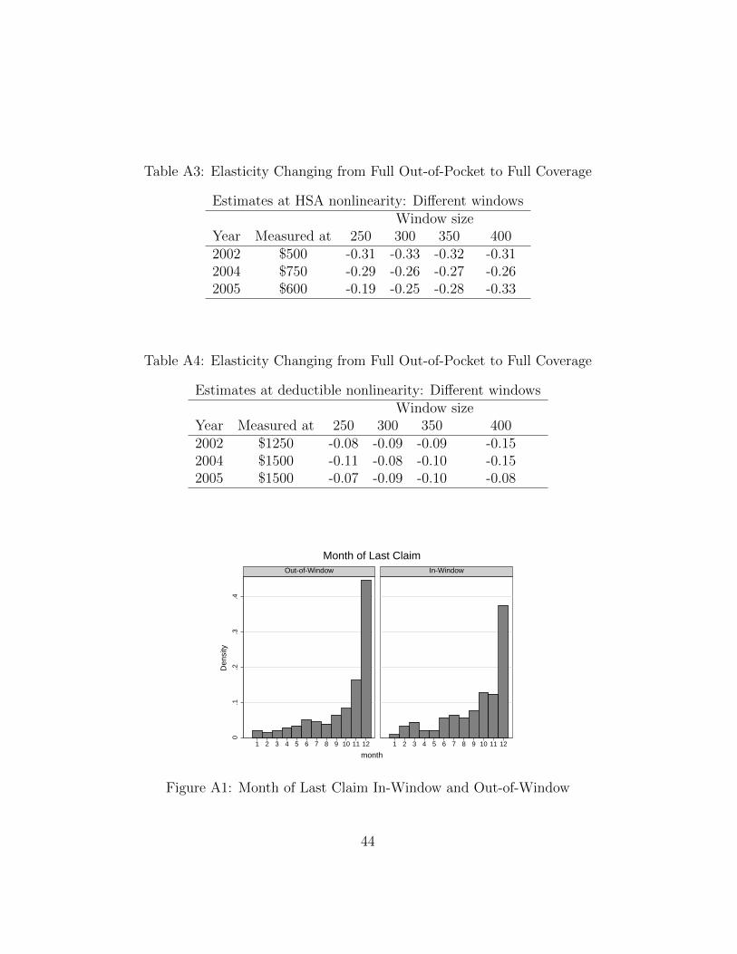
Table A3: Elasticity Changing from Full Out-of-Pocket to Full Coverage

Estimates at HSA nonlinearity: Different windowsWindow size

Year Measured at 250 300 350 4002002 $500 -0.31 -0.33 -0.32 -0.312004 $750 -0.29 -0.26 -0.27 -0.262005 $600 -0.19 -0.25 -0.28 -0.33

Table A4: Elasticity Changing from Full Out-of-Pocket to Full Coverage

Estimates at deductible nonlinearity: Different windowsWindow size

Year Measured at 250 300 350 4002002 $1250 -0.08 -0.09 -0.09 -0.152004 $1500 -0.11 -0.08 -0.10 -0.152005 $1500 -0.07 -0.09 -0.10 -0.08

0.1

.2.3

.4

1 2 3 4 5 6 7 8 9 10 11 12 1 2 3 4 5 6 7 8 9 10 11 12

Out-of-Window In-Window

Den

sity

month

Month of Last Claim

Figure A1: Month of Last Claim In-Window and Out-of-Window

44

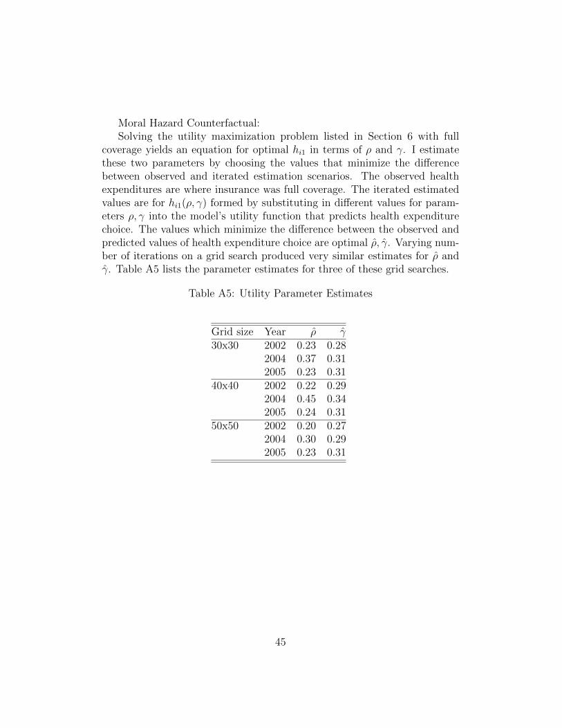
Moral Hazard Counterfactual:Solving the utility maximization problem listed in Section 6 with full

coverage yields an equation for optimal hi1 in terms of ρ and γ. I estimatethese two parameters by choosing the values that minimize the differencebetween observed and iterated estimation scenarios. The observed healthexpenditures are where insurance was full coverage. The iterated estimatedvalues are for hi1(ρ, γ) formed by substituting in different values for param-eters ρ, γ into the model’s utility function that predicts health expenditurechoice. The values which minimize the difference between the observed andpredicted values of health expenditure choice are optimal ρ̂, γ̂. Varying num-ber of iterations on a grid search produced very similar estimates for ρ̂ andγ̂. Table A5 lists the parameter estimates for three of these grid searches.

Table A5: Utility Parameter Estimates

Grid size Year ρ̂ γ̂30x30 2002 0.23 0.28

2004 0.37 0.312005 0.23 0.31

40x40 2002 0.22 0.292004 0.45 0.342005 0.24 0.31

50x50 2002 0.20 0.272004 0.30 0.292005 0.23 0.31

45

In this appendix, I lay out a flexible parametric form for the utility func-tion of the patient and solve explicitly for the patient’s decision rule.

Consider the following general utility function which satisfies utility con-ditions (1) - (5) from Section 2:

U(h, θ, c) = u(h, θ) + c

= γθ + αθhβ − τh+ c (A1)

Where γ is a parameter on the health shock, α is the parameter on theinteraction of the health shock and health expenditures, β is the patient’srisk parameter, and τ is the parameter on the time inconvenience from goingto the doctor or from utility-reducing levels of health care.

Utility conditions (1), (3), and (5) are clearly satisfied. Condition (2)

is satisfied with hmaxθ =[αβθτ

] 11−β . Condition (4) is satisfied with γ small

enough, such that γ < αhβ.The corresponding optimal decision rule is:

h∗ =

[αβθ

1− p+ τ

] 11−β

(A2)

Recall the reimbursement schedule with a deductible, h̄, and resultingMC schedule as described in Section 2:

MC = 1− p =

{1 if h ≤ h̄

0 if h > h̄

Given the reimbursement schedule and a health status of θ, the corre-sponding optimal h∗ in each marginal cost section is:

h∗ =

[αβθτ+1

] 11−β if h∗ ≤ h̄[

αβθτ

] 11−β if h∗ > h̄

(A3)

Notice that the optimal h∗ that is chosen in the first part of the reimburse-ment schedule, where all health expenditure must be paid fully out-of-pocket,is smaller than the h∗ that is chosen in the second part of the reimbursementschedule, where all additional units of expenditure are fully covered by theinsurance plan.

Because the decision rule for the choice of h is strictly increasing in θ asθ approaches the nonlinearity, the decision rule can be written in terms of

46

θ̄, where θ̄ is the value of θ that corresponds to the nonlinearity, h̄. For thisreason, the indicator function 1{h ≤ h̄} can be written as 1{θ ≤ θ̄}, and viceversa for the right-hand side of the nonlinearity.

Equation A3 can be transformed into a linear equation using a Taylorapproximation around θ̄. The linear approximation is:

h =

[αβθ̄

τ + 1{θ ≤ θ̄}

] 11−β

+1

1− β

[αβθ̄β

τ + 1{θ ≤ θ̄}

] 11−β

(θ − θ̄) (A4)

To construct a local linear regression from Equation A4, estimation occursin the neighborhood of the θ̄ term, with the following coefficients:

a(θ) =

[αβθ̄

τ + 1{θ ≤ θ̄}

] 11−β

b(θ) =1

1− β

[αβθ̄β

τ + 1{θ ≤ θ̄}

] 11−β

47