estimating air pollution and its relationship with human...
TRANSCRIPT

Glasgow Theses Service http://theses.gla.ac.uk/
Powell, Helen Louise (2012) Estimating air pollution and its relationship with human health. PhD thesis http://theses.gla.ac.uk/3531/ Copyright and moral rights for this thesis are retained by the author A copy can be downloaded for personal non-commercial research or study, without prior permission or charge This thesis cannot be reproduced or quoted extensively from without first obtaining permission in writing from the Author The content must not be changed in any way or sold commercially in any format or medium without the formal permission of the Author When referring to this work, full bibliographic details including the author, title, awarding institution and date of the thesis must be given.

UNIVERSITY OF GLASGOW
Estimating Air Pollution and its
Relationship with Human Health
by
Helen Louise Powell
A thesis submitted in fulfillment for the
degree of Doctor of Philosophy
in the
School of Mathematics and Statistics
College of Science and Engineering
July 2012

Declaration of Authorship
I, Helen Powell, declare that this thesis titled, ‘Estimating Air Pollution and its
Relationship with Human Health’ and the work presented in it are my own. I
confirm that where I have consulated the published work of others, this is always
clearly attributed. Where I have quoted from the work of others, the source is
always given. With the exception of such quotations, this thesis is entirely my
own work.
The work presented in Chapter 4 is currently under review with the Journal of
the Royal Statistical Society Series A with the title Estimating overall air quality
and its effects on human health in Greater London. The same work has also been
presented at the 58th World Statistics Congress of the International Statistical
Institute (ISI) in Dublin, 2011, with the title Estimating overall air quality and its
effects on human health.
The work presented in Chapter 6 has been published in Environmetrics with the
title Estimating constrained concentration-response functions between air pollution
and health, and is jointly authored with Duncan Lee and Adrian Bowman (DOI:
10.1002/env.1150). The same work has also been presented at the 25th Inter-
national Workshop on Statistical Modelling (IWSM) in Glasgow, 2010, with the
title Estimating biologically plausible relationships between air pollution and health.
i

“We’ve got to pause and ask ourselves: How much clean air do we need?”
Lee Lacocca, CEO/Chairman, Chrysler Corporation, 1979-1992

Abstract
The health impact of short-term exposure to air pollution has been the focus of
much recent research, the majority of which is based on time-series studies. A
time-series study uses health, pollution and meteorological data from an extended
urban area. Aggregate level data is used to describe the health of the population
living with the region, this is typically a daily count of the number of mortality
or morbidity events. Air pollution data is obtained from a number of fixed site
monitors located throughout the study region. These monitors measure back-
ground pollution levels at a number of time intervals throughout the day and a
daily average is typically calculated for each site. A number of pollutants are
measured including, carbon monoxide (CO); nitrogen dioxide (NO2); particulate
matter (PM2.5 and PM10), and; sulphur dioxide (SO2). These fixed site monitors
also measure a number of meteorological covariates such as temperature, humidity
and solar radiation. In this thesis I have presented extensions to the current meth-
ods which are used to estimate the association between air pollution exposure and
the risks to human health. The comparisons of the efficacy of my approaches to
those which are adopted by the majority of researchers, highlights some of the de-
ficiencies of the standard approaches to modelling such data. The work presented
here is centered around three specific themes, all of which focus on the air pollu-
tion component of the model. The first and second theme relate to what is used
as a spatially representative measure of air pollution and allowing for uncertainty
in what is an inherently unknown quantity, when estimating the associated health
risks, respectively. For example the majority of air pollution and health studies
only consider the health effects of a single pollutant rather than that of overall
air quality. In addition to this, the single pollutant estimate is taken as the aver-
age concentration level across the network of monitors. This is unlikely to be the
average concentration across the study region due to the likely non random place-
ment of the monitoring network. To address these issues I proposed two methods

for estimating a spatially representative measure of pollution. Both methods are
based on hierarchical Bayesian methods, as this allows for the correct propagation
of uncertainty, the first of which uses geostatistical methods and the second is a
simple regression model which includes a time-varying coefficient for covariates
which are fixed in space. I compared the two approaches in terms of their pre-
dictive accuracy using cross validation. The third theme considers the shape of
the estimated concentration-response function between air pollution and health.
Currently used modelling techniques make no constraints on such a function and
can therefore produce unrealistic results, such as decreasing risks to health at high
concentrations. I therefore proposed a model which imposes three constraints on
the concentration-response function in order to produce a more sensible shaped
curve and therefore eliminate such misinterpretations. The efficacy of this ap-
proach was assessed via a simulation study. All of the methods presented in this
thesis are illustrated using data from the Greater London area.

Acknowledgements
So many of you have helped and supported me that I couldn’t possibly start to
thank you all individually, so instead let me just say, Thank You, I am truly
grateful.
v

Contents
Declaration of Authorship i
Abstract iii
Acknowledgements v
List of Figures x
List of Tables xiii
1 Introduction 1
2 Statistical Methods Review 10
2.1 Frequentist Methods . . . . . . . . . . . . . . . . . . . . . . . . . . 11
2.1.1 The Exponential Family . . . . . . . . . . . . . . . . . . . . 12
2.1.2 Maximum Likelihood Estimation . . . . . . . . . . . . . . . 13
2.1.3 Confidence Intervals . . . . . . . . . . . . . . . . . . . . . . 15
2.2 Bayesian Methods . . . . . . . . . . . . . . . . . . . . . . . . . . . . 16
2.2.1 The Prior Distribution . . . . . . . . . . . . . . . . . . . . . 17
2.2.2 Inference . . . . . . . . . . . . . . . . . . . . . . . . . . . . . 18
2.3 Spatial Data and Geostatistics . . . . . . . . . . . . . . . . . . . . . 21
2.3.1 Geostatistics . . . . . . . . . . . . . . . . . . . . . . . . . . . 23
2.3.1.1 Parameter Estimation and Spatial Prediction . . . 25
2.4 Varying-Coefficient Models . . . . . . . . . . . . . . . . . . . . . . . 30
2.4.1 Time-Varying Coefficient Models . . . . . . . . . . . . . . . 31
2.4.2 Estimation . . . . . . . . . . . . . . . . . . . . . . . . . . . . 32
2.5 Regression Splines . . . . . . . . . . . . . . . . . . . . . . . . . . . 32
2.5.1 Building Regression Splines . . . . . . . . . . . . . . . . . . 33
2.5.2 Basis Functions . . . . . . . . . . . . . . . . . . . . . . . . . 35
2.6 Model Selection, Assessment and Prediction . . . . . . . . . . . . . 37
vi

Contents vii
2.6.1 Model Selection . . . . . . . . . . . . . . . . . . . . . . . . . 38
2.6.1.1 Measures of Model Fit . . . . . . . . . . . . . . . . 38
2.6.2 Model Assessment . . . . . . . . . . . . . . . . . . . . . . . 40
2.6.2.1 Standardised Residuals . . . . . . . . . . . . . . . . 41
2.6.2.2 Measuring Model Adequacy . . . . . . . . . . . . . 42
2.6.2.3 Posterior Predictive Checking . . . . . . . . . . . . 43
2.6.2.4 Sensitivity Analysis . . . . . . . . . . . . . . . . . . 44
2.6.3 Model Prediction . . . . . . . . . . . . . . . . . . . . . . . . 44
3 Air Pollution and Health Studies 47
3.1 Data Description . . . . . . . . . . . . . . . . . . . . . . . . . . . . 47
3.1.1 Health Data . . . . . . . . . . . . . . . . . . . . . . . . . . . 48
3.1.2 Air Pollution Data . . . . . . . . . . . . . . . . . . . . . . . 50
3.1.3 Other Covariates . . . . . . . . . . . . . . . . . . . . . . . . 54
3.2 Examining Air Pollution . . . . . . . . . . . . . . . . . . . . . . . . 55
3.2.1 Representing Air Quality . . . . . . . . . . . . . . . . . . . . 56
3.2.1.1 Selecting a Pollutant . . . . . . . . . . . . . . . . . 56
3.2.1.2 Measuring Pollution . . . . . . . . . . . . . . . . . 58
3.2.2 The Pollution-health Relationship . . . . . . . . . . . . . . . 59
3.2.3 Lag . . . . . . . . . . . . . . . . . . . . . . . . . . . . . . . . 61
3.3 Covariate Specification . . . . . . . . . . . . . . . . . . . . . . . . . 63
3.3.1 Measured Confounders . . . . . . . . . . . . . . . . . . . . . 63
3.3.2 Unmeasured Confounders . . . . . . . . . . . . . . . . . . . 65
3.4 Overdispersion . . . . . . . . . . . . . . . . . . . . . . . . . . . . . 67
3.5 Mortality Displacement . . . . . . . . . . . . . . . . . . . . . . . . . 68
4 Estimating Overall Air Quality using Geostatistical Methods 71
4.1 Motivation . . . . . . . . . . . . . . . . . . . . . . . . . . . . . . . . 72
4.2 Background . . . . . . . . . . . . . . . . . . . . . . . . . . . . . . . 74
4.3 Methods . . . . . . . . . . . . . . . . . . . . . . . . . . . . . . . . . 75
4.3.1 Pollution Model (single pollutant) . . . . . . . . . . . . . . . 76
4.3.2 Aggregation Model . . . . . . . . . . . . . . . . . . . . . . . 78
4.3.3 Health Model . . . . . . . . . . . . . . . . . . . . . . . . . . 80
4.4 Application - Greater London . . . . . . . . . . . . . . . . . . . . . 81
4.4.1 Data . . . . . . . . . . . . . . . . . . . . . . . . . . . . . . . 81
4.4.1.1 Pollution Data . . . . . . . . . . . . . . . . . . . . 83
4.4.1.2 Health Data . . . . . . . . . . . . . . . . . . . . . . 85
4.4.1.3 Population Data . . . . . . . . . . . . . . . . . . . 87
4.4.2 Statistical Modelling . . . . . . . . . . . . . . . . . . . . . . 89
4.4.2.1 Pollution Modelling . . . . . . . . . . . . . . . . . 89
4.4.2.2 Health Modelling . . . . . . . . . . . . . . . . . . . 90

Contents viii
4.4.3 Results . . . . . . . . . . . . . . . . . . . . . . . . . . . . . . 92
4.4.3.1 Pollution Model Results . . . . . . . . . . . . . . . 92
4.4.3.2 Health Model Results . . . . . . . . . . . . . . . . 94
4.5 Discussion . . . . . . . . . . . . . . . . . . . . . . . . . . . . . . . . 95
5 Estimating Overall Air Quality using Bayesian Regression Anal-ysis 102
5.1 Introduction . . . . . . . . . . . . . . . . . . . . . . . . . . . . . . . 102
5.2 Methods . . . . . . . . . . . . . . . . . . . . . . . . . . . . . . . . . 104
5.2.1 Pollution Model (single pollutant) . . . . . . . . . . . . . . . 105
5.2.2 Aggregation Model . . . . . . . . . . . . . . . . . . . . . . . 110
5.2.3 Health Model . . . . . . . . . . . . . . . . . . . . . . . . . . 111
5.3 Model Validation . . . . . . . . . . . . . . . . . . . . . . . . . . . . 112
5.3.1 Results . . . . . . . . . . . . . . . . . . . . . . . . . . . . . . 113
5.4 Application - Greater London . . . . . . . . . . . . . . . . . . . . . 117
5.4.1 Description of Data . . . . . . . . . . . . . . . . . . . . . . . 117
5.4.1.1 Pollution Data . . . . . . . . . . . . . . . . . . . . 117
5.4.1.2 Meteorological data . . . . . . . . . . . . . . . . . 121
5.4.2 Statistical Modelling . . . . . . . . . . . . . . . . . . . . . . 123
5.4.2.1 Pollution Modelling . . . . . . . . . . . . . . . . . 123
5.4.2.2 Health Modelling . . . . . . . . . . . . . . . . . . . 125
5.4.3 Results . . . . . . . . . . . . . . . . . . . . . . . . . . . . . . 126
5.4.3.1 Pollution Model Results . . . . . . . . . . . . . . . 126
5.4.3.2 Health Model Results . . . . . . . . . . . . . . . . 134
5.5 Discussion . . . . . . . . . . . . . . . . . . . . . . . . . . . . . . . . 136
6 Estimating Constrained Concentration-Response Functions 140
6.1 Introduction . . . . . . . . . . . . . . . . . . . . . . . . . . . . . . . 140
6.2 Background and Motivation . . . . . . . . . . . . . . . . . . . . . . 141
6.2.1 Air Pollution and Health Studies . . . . . . . . . . . . . . . 142
6.2.2 Constrained Concentration-Response Functions . . . . . . . 143
6.3 Methods . . . . . . . . . . . . . . . . . . . . . . . . . . . . . . . . . 146
6.3.1 Modelling the Concentration-Response Function f(·) . . . . 146
6.3.2 Bayesian Model and Estimation . . . . . . . . . . . . . . . . 149
6.4 Simulation Study . . . . . . . . . . . . . . . . . . . . . . . . . . . . 153
6.4.1 Study Design and Data Generation . . . . . . . . . . . . . . 153
6.4.2 Results . . . . . . . . . . . . . . . . . . . . . . . . . . . . . . 155
6.5 Application - Greater London . . . . . . . . . . . . . . . . . . . . . 157
6.5.1 Data . . . . . . . . . . . . . . . . . . . . . . . . . . . . . . . 160
6.5.2 Statistical Modelling . . . . . . . . . . . . . . . . . . . . . . 162
6.5.3 Results . . . . . . . . . . . . . . . . . . . . . . . . . . . . . . 163

Contents ix
6.6 Discussion . . . . . . . . . . . . . . . . . . . . . . . . . . . . . . . . 165
7 Conclusion 169
7.1 Key Theme - Estimating a spatially representative measure of over-all air quality . . . . . . . . . . . . . . . . . . . . . . . . . . . . . . 171
7.1.1 Related Theme - Allowing for uncertainty when estimatingthe health risks of air pollution . . . . . . . . . . . . . . . . 175
7.2 Key Theme - Constraining the relationship between air pollutionand health . . . . . . . . . . . . . . . . . . . . . . . . . . . . . . . . 176
7.2.1 Limitations . . . . . . . . . . . . . . . . . . . . . . . . . . . 178

List of Figures
1.1 Concentrations of smoke, sulphur dioxide (SO2), and daily respira-tory deaths for the period surrounding the London smog of 1952(www.ems.psu.edu). . . . . . . . . . . . . . . . . . . . . . . . . . . . 3
2.1 B-spline bases of degrees (a) one, (b) two, and (c) three. The po-sition of the knots are indicated by the solid diamonds (taken fromWand (2000)). . . . . . . . . . . . . . . . . . . . . . . . . . . . . . . 35
2.2 Natural cubic spline basis for the same set of knots used in Figure2.1 (taken from Wand (2000)). . . . . . . . . . . . . . . . . . . . . . 36
3.1 (a) Daily counts of the number of respiratory related mortalitiesfrom the population of over 65s living in Greater London for theperiod 2001 to 2003, (b) daily average temperature for the same re-gion and period, and (c) the relationship between the daily averagetemperature and the number of respiratory related deaths, wherethe shaped of the relationship has been highlighted by the red line. 49
3.2 Location and type of the pollution monitors in Greater London (•,roadside locations; , background locations): (a) CO, (b) NO2, (c)O3, and (d) PM10. . . . . . . . . . . . . . . . . . . . . . . . . . . . 51
3.3 The hypothetical lag structure corresponding to the mortality dis-placement effect. Taken from Zanobetti et al. (2000)) . . . . . . . . 69
4.1 Location and type of the pollution monitors in Greater London, forwhich the percentage of missing data for the period 2001 to 2003 isno more than 25% (•, roadside locations; , background locations):(a) CO, (b) NO2, (c) O3, (d) PM10, and (e) the prediction locations. 82
4.2 Maps of the 1 kilometre modelled estimates of the yearly averageconcentration for (a) CO, (b) NO2 and (c) PM10, in 2001. . . . . . . 85
4.3 (a) Daily counts of the number of respiratory related mortalitiesfrom the population of over 65s living in Greater London for theperiod 2001 to 2003, (b) daily average temperature for the same re-gion and period, and (c) the relationship between the daily averagetemperature and the number of respiratory related deaths, wherethe shaped of the relationship has been highlighted by the red line. 86
x

List of Figures xi
4.4 Map of the 1 kilometre population count of the over 65s living inGreater London at the time of 2001 census. . . . . . . . . . . . . . . 87
4.5 Average concentration, for the period 2001 to 2003, recorded ateach monitoring site against the associated easting and northingcoordinates for CO (a and b), NO2 (c and d), O3 (e and f), andPM10 (g and h). . . . . . . . . . . . . . . . . . . . . . . . . . . . . . 88
4.6 The residuals of the health model (4.6) (a), the autocorrelationfunction, ACF (b), and partial autocorrelation function, PACF(c) . 100
4.7 Posterior medians (•) and 95% credible intervals ( | ) from thegeostatistical model and the monitor average for the individual pol-lutants (a) CO, (b) NO2, (c) O3, (d) PM10 and (e) the air qualityindicator. . . . . . . . . . . . . . . . . . . . . . . . . . . . . . . . . 101
5.1 Locations of the training (black) and validation (red) PM10 mon-itoring sites within Greater London, used in each of the 5 (a - e)test cases (•, roadside locations; , background locations). . . . . . 114
5.2 Location and type of the pollution monitors in Greater London (•,roadside locations; , background locations): (a) CO, (b) NO2, (c)O3, (d) PM10, and (e) the prediction locations. . . . . . . . . . . . . 118
5.3 The daily average rural (red) and observed concentrations (black)for (a) NO2, (b) O3 and (c) PM10. . . . . . . . . . . . . . . . . . . . 122
5.4 Posterior medians (•) and 95% credible intervals ( | ) from theregression model without a time-varying coefficient and the monitoraverage for the individual pollutants (a) CO, (b) NO2, (c) O3, (d)PM10 and (e) the air quality indicator (AQI). . . . . . . . . . . . . 127
5.5 The results of the 20,000 MCMC simulations for the variance pa-rameter σ2, less the burn-in period, proposed by the regressionmodel without a time-varying coefficient. . . . . . . . . . . . . . . 129
5.6 The results of the 20,000 MCMC simulations for the variance pa-rameter σ2, less the burn-in period, proposed by the regressionmodel with a time-varying coefficient. . . . . . . . . . . . . . . . . . 131
5.7 Posterior medians (•) and 95% credible intervals ( | ) from theregression model with a time-varying coefficient and the monitoraverage for the individual pollutants (a) CO, (b) NO2, (c) PM10,and (d) the air quality indicator (AQI). . . . . . . . . . . . . . . . . 132
6.1 A set of five M-spline basis functions of order (a) 1, (b) 2 and (c)3, and (d) a set of five I-spline basis functions of cubic (3) order. . . 147
6.2 The true CRFs for the four scenarios: (1) a linear CRF (solidblack line), (2) a constant CRF (solid gray line), (3) a convex CRF(dashed line), and (d) a concave CRF (dotted line). . . . . . . . . . 154

List of Figures xii
6.3 Percentage bias for each model and scenario at concentrations rang-ing between 0 and 90 microns. The four rows depict the results fromthe four scenarios. . . . . . . . . . . . . . . . . . . . . . . . . . . . . 158
6.4 Percentage median absolute deviation for each model and scenarioat concentrations ranging between 0 and 90 microns. The four rowsdepict the results from the four scenarios. . . . . . . . . . . . . . . . 159
6.5 Daily counts of (a) respiratory deaths, (b) pollution concentrationsand (c) average temperature in Greater London for the period 2000to 2005. . . . . . . . . . . . . . . . . . . . . . . . . . . . . . . . . . 161
6.6 Relative risk curves and associated 95% confidence (credible) inter-vals for: (a) a linear relationship; (b) the B-spline model; (c) theBayesian I-spline model; and (d) the piecewise linear model. . . . . 166

List of Tables
4.1 Summary of the pollution data, including the mean and both thetemporal and spatial standard deviation. . . . . . . . . . . . . . . . 84
4.2 Temporal summary of the population weighted average pollutantconcentrations. . . . . . . . . . . . . . . . . . . . . . . . . . . . . . 93
4.3 Relative risks and 95% uncertainty intervals. . . . . . . . . . . . . . 95
5.1 The PB and MAD scores, relative to observed PM10, for the regres-sion model (5.1), without and with a time-varying coefficient, andthe geostatistical model, presented in Chapter 4. . . . . . . . . . . . 115
5.2 Summary of the pollution data, including the temporal mean andboth the temporal and spatial standard deviation. . . . . . . . . . . 120
5.3 Summary of the daily rural pollution concentrations and the mete-orological data, available for Greater London in the period 2001 to2003. . . . . . . . . . . . . . . . . . . . . . . . . . . . . . . . . . . . 123
5.4 Summary of the posterior predictive distributions found when im-plementing the regression model with no time-varying coefficient. . 130
5.5 Summary of the posterior predictive distributions found when im-plementing the regression model with a time-varying coefficient. . . 133
5.6 Relative risks and 95% uncertainty intervals. . . . . . . . . . . . . . 135
6.1 Summary of the simulation study. The table displays the bias,median absolute deviation and the percentage of estimated CRFsthat are biologically plausible, for each model and scenario. . . . . . 156
xiii

Chapter 1
Introduction
Short-term exposure to air pollution can cause and aggravate a number of respira-
tory conditions, including asthma, bronchitis and chronic obstructive pulmonary
disease (COPD). This association between air pollution exposure and the risks to
human health has been a public health concern for over 700 years. King Edward I
of England outlawed the burning of coal and made it punishable by death in 1306,
when petitioned to do so by a large group of affluent people and the clergy. The
King’s decision may also have been influenced by his mother, Queen Eleanor, who
became unwell as a result of the coal fumes rising up to the castle from the town
below. Approximately 250 years later the air quality in England once again grew
noticeably worse and Queen Elizabeth was also forced to ban the burning of coal.
Despite this early recognition of the health risks associated with poor air quality
it has only become a global topic in the last 80 years. This has primarily been due
to the exceptionally high air pollution episodes in the Meuse Valley in 1930 (Fir-
ket (1936)), in Donora, Pennsylvania in 1948 (Ciocco and Thompson (1961)) and
during the London smog of December 1952 (Ministry of Public Health (1954)).
These episodes were caused by a combination of industrial pollution sources and
adverse weather conditions, and resulted in a large number of premature deaths
among the surrounding populations. For example, as highlighted in Figure 1.1,
1
Chapter 1. Introduction 2
the London smog was associated with a significant rise in the number of respira-
tory deaths in December 1952 when compared with the number of deaths in the
surrounding period. It has even been suggested that the number of deaths during
the smog, and in the subsequent two months was in fact closer to 12,000 (Bell
and Davies (2001)). Despite pollution levels being considerably lower in the last
20 years than those witnessed in the episodes described above, the relationship
between air pollution and morbidity or mortality continues to be an active area
of research. Evidence from such studies has helped shape environmental legisla-
tion, which regulates the sources of pollution and sets target limits for ambient
(outdoor) concentrations. In the UK such legislation includes the Clean Air Act
in 1993 and the UK Air Quality Strategy in 2007, with the latter, for example,
stipulating that particulate matter (PM10) must not exceed 40µgm−3 as an annual
mean.
The majority of air pollution and health studies examine the effects of short-term
(acute) exposure over a few days, rather than long-term (chronic) exposure over
a number of years. To estimate the health risks of chronic exposure a cohort
study is typically used. For example Dockery et al. (1993) examined the output
of a cohort study in which over 8000 adults in six U.S. cities (HSCS, Harvard Six
Cities Study) were followed for a period of 14-16 years. Other examples of cohort
studies include the American Cancer Study (Pope III et al. (1995) and Pope III
et al. (2002)) which collected data on approximately 1.2 million adults in 1982,
and the Millenium Cohort Study (Violato et al. (2009)) in the U.K. which sampled
nearly 19,000 babies born in England and Wales between 2000 and 2002. Cohort
studies are not frequently used due to the scale of the sampling and the associ-
ated costs. Therefore, the majority of studies examine the relationship between
acute exposure and mortality or morbidity. These studies can be broadly classi-
fied into three categories: case-crossover studies (Neas et al. (1999) and Ma et al.
(2011)), panel studies (Sarnat et al. (2012)), and time-series studies (Alessandrini

Chapter 1. Introduction 3
Figure 1.1: Concentrations of smoke, sulphur dioxide (SO2), and dailyrespiratory deaths for the period surrounding the London smog of 1952
(www.ems.psu.edu).
et al. (2011) and Dominici et al. (2006)). Both case-crossover and panel studies
use data at an individual level allowing an exposure-response relationship to be
estimated. However, being able to specifically classify a mortality or morbidity
event as pollution related is rare, and a large number of individuals would be re-
quired in order to produce conclusive results. Therefore, the majority of research
on the health implications of air pollution is based on time-series studies. Such
studies use aggregate level mortality or morbidity data, which describe the health
of the population living within a geographical region rather than that of specific
individuals. This type of data is routinely available, making this type of study

Chapter 1. Introduction 4
inexpensive and straightforward to implement. Another advantage of time-series
analysis is that it is unlikely to be affected by individual level risk factors such as
age and smoking habits, as these are likely to be constant over the study period. A
disadvantage is that only group level associations between air pollution exposure
and health can be estimated, which is a much weaker type of analysis than an
individual exposure-response relationship (see for example Wakefield and Salway
(2001)). This thesis will focus on time-series studies, but for a more general review
of air pollution and health studies see (Pope III and Dockery (2006) and Dominici
et al. (2003)).
A time-series study is based on health, pollution and meteorological data from
an extended urban area such as a city. The health data comprise daily counts
of mortality or morbidity outcomes for the population living within the study re-
gion. A number of health classifications have been used in such studies, including
general categories such as total non-accidental mortality (Kan et al. (2007)), and
illness specific subclasses such as respiratory mortality and hospital admissions
due to asthma (Sarnat et al. (2012)). Data which contributes to air pollution
are obtained from a number of fixed-site monitors, located throughout the study
region. These monitors measure background pollution levels throughout the day
and a daily average is typically calculated at each site. A number of pollutants
are typically measured including, carbon monoxide (CO); nitrogen dioxide (NO2);
particulate matter (PM10 and PM2.5), and; sulphur dioxide (SO2). Finally, mete-
orological covariates such as temperature, humidity and solar radiation, are also
routinely measured by fixed-site monitors.
Schwartz and Marcus (1990) were one of the first to carry out a time-series study
of the health risks of air pollution. They used a normal linear model to analyse
data from the Greater London area. However, the mortality or morbidity data

Chapter 1. Introduction 5
are daily counts and often include small numbers, therefore Poisson regression
techniques such as generalized linear (GLM, McCullagh and Nelder (1989)) or ad-
ditive (GAM, Hastie and Tibshirani (1990)) models are more appropriate. These
models regress the daily counts of mortality or morbidity events against air pol-
lution concentrations and a vector of explanatory covariates. These covariates are
included to remove the effects of confounding which are introduced through under-
lying trends, seasonal patterns and overdispersion. Typically included variables
are measures of meteorological conditions, influenza epidemic indicators and day
of the week indicators. Air pollution studies often analyse data from a number
of cities (see for example Schwartz (1991) and Spix et al. (1993)), using a variety
of statistical approaches. This variation in statistical methodology may be partly
responsible for the considerable heterogeneity observed in the pollution-health as-
sociations which have been estimated. A number of researchers have attempted to
reduce this heterogeneity by implementing large multi-city studies, including Air
Pollution and Health: A European Approach (APHEA, see for example Samoli
et al. (2009)), and the National Morbidity, Mortality and Air Pollution Study
(NMMAPS, see for example Huang et al. (2005)) in the USA. These studies ease
the comparison between multiple cities by using standard modelling approaches.
In this thesis I extend the current methods used to estimate the association be-
tween air pollution exposure and the risks to human health, and compare their
efficacy against those adopted by the majority of researchers. These developments
provide evidence of deficiencies with the standard approaches to modelling such
data. The work presented in this thesis is centered around three related themes,
which focus on the air pollution component of the regression model. The first and
second themes relate to the measure of ambient air pollution which is included in
the model. The majority of studies typically estimate the short term health effects
of exposure to a single pollutant. I compare this approach to the health effects of
overall air quality which is the quantity that the population are actually exposed
Chapter 1. Introduction 6
to. The second theme is to allow for uncertainty in the pollution estimate and
compare the effect this has on the estimated health risks of overall air pollution.
The third theme considers the shape of the estimated concentration-response func-
tion between air pollution and health. The modelling techniques currently utilised
make no constraints on such a function and as a result can produce unrealistic
results. For example the estimated function may exhibit decreases in the risks
to health at high concentrations. In this thesis I propose a model which imposes
three constraints on the concentration-response function in order to produce a
more sensible shaped curve and therefore eliminate such misinterpretations. The
work in each of these themes has been carried out using Bayesian techniques.
The remainder of this thesis has been arranged into six chapters, the first of which
reviews and critiques the statistical methodology typically used in current air pol-
lution and health studies. Chapter 3 discusses some of the statistical issues which
arise in air pollution and health studies. Chapter 4 defines a spatially representa-
tive measure of a single pollutant, on a single day, which can be estimated using
Bayesian geostatistical methods. This is then repeated for several pollutants which
are then combined to give a single measure of overall air quality. This process is
repeated for each day of the study period, and the health risks of this overall
measure are then estimated and compared to that of the standard approach. By
drawing a random sample from the posterior distribution of predictions of overall
air quality for each day, it is possible to incorporate the uncertainty about the
true pollution levels for that day into the health model. Chapter 5 considers an
alternative approach for estimating such a spatially representative measure of air
pollution, by utilising a regression model for the data in space and time simul-
taneously. This model is made more flexible by the inclusion of a time-varying
coefficient which will allow the effects of covariates which are fixed in space but
believed to vary over time. Again the associated health risks for such a measure
are estimated and compared to that of the standard approach. I compare the

Chapter 1. Introduction 7
efficacy of this approach to that of the geostatistical model used in the previous
section using the method of cross validation, a tool for determining the predictive
accuracy of a model. Chapter 6 considers which constraints are necessary in order
to produce a sensible concentration-response function between air pollution and
health. A constrained model is built using I-splines and is compared to the stan-
dard approach of using B-splines and that of another constrained method which
was proposed by Roberts (2004). The remainder of this introduction describes the
individual chapters in more detail.
Chapter 2 reviews the statistical methods which are used in current air pollution
and health studies and also in this thesis. Both frequentist and Bayesian analysis
are outlined, including a review of the estimation techniques; maximum likeli-
hood and Markov chain Monte Carlo simulation. Although this thesis uses only
Bayesian analysis a review of frequentist approaches has been included, as this
is predominantly the analysis method used in the majority of air pollution and
health studies. I have included a review of geostatistics, time-varying coefficient
models and regression splines, as background knowledge for the methods used in
Chapters 4, 5 and 6 respectively. This chapter also includes a review of model
selection criteria.
In Chapter 3 I discuss some of the statistical issues which arise in air pollution
and health studies. This includes a discussion of the type of data typically used in
such studies. Particular attention is given to the air pollution data including what
is typically included as a spatially representative measure of air quality and how
this measure enters the model. This particular aspect of air pollution and health
studies forms the basis of all the work presented in this thesis. Both measured and
unmeasured covariates are discussed. This chapter concludes with a discussion of
the problems of overdispersion and mortality displacement.

Chapter 1. Introduction 8
Chapter 4 considers that most studies typically only assess the health risks of
a single pollutant rather than that of overall air quality. In addition, these sin-
gle pollutant levels are estimated by averaging measurements across a network of
monitors and this simplistic method of estimation has a number of deficiencies.
Firstly, it is unlikely to be the average concentration across the region under study,
due to the likely non-random placement of the monitoring network. Secondly, the
desired pollution measure is inherently an unknown quantity, and hence the un-
certainty in any estimate should be allowed for when estimating its health risks. I
address these issues, and propose both a spatially representative measure of overall
air quality, and a corresponding health model that allows for the uncertainty in
the pollution estimate. My approach is based on a hierarchical Bayesian model
because it allows for the correct propagation of uncertainty, and uses geostatistical
methods to estimate a spatially representative measure of pollution. The methods
are illustrated by assessing the health impacts of overall air quality in Greater
London between 2001 and 2003.
Chapter 5 considers that some of the more complex methods for building a spa-
tially representative measure of air pollution, including that proposed in the previ-
ous chapter, can be computationally expensive as separate Bayesian geostatistical
models are fitted for each day of the study. Another approach would be to model
air pollution over time and space simultaneously using regression analysis. I have
proposed such a model and also included a time-varying coefficient, which will
allow the effects of spatial covariates to evolve over time, thus increasing the flex-
ibility of the model. A hierarchical Bayesian model is also proposed here to allow
for the correct propagation of the uncertainty in the pollution estimate. These
methods are illustrated by assessing the health impacts of overall air quality in
Greater London for the period 2001 to 2003.

Chapter 1. Introduction 9
Chapter 6 considers how the assumption of linearity between air pollution expo-
sure and risks to health can be relaxed and yet impose constraints on the shape of
the estimated concentration-response function (CRF) so as to produce feasible re-
sults. I therefore propose a Bayesian hierarchical model for estimating constrained
concentration-response functions, which is based on monotonic integrated splines.
These splines produce non-decreasing CRFs, due to the associated regression pa-
rameters being constrained to be non-negative, which I ensure by modelling the
latter with a ‘slab and spike’ prior. I assess the efficacy of my approach via a
simulation study, after which I apply the proposed model to a study of ozone con-
centrations and respiratory disease in Greater London between 2000 and 2005.
Chapter 7 discusses the main results from this thesis and assess its contribution
to the wider literature. The limitations of the work are discussed, with possible
extensions and future work outlined.
Chapter 2
Statistical Methods Review
The adverse health risks associated with ambient air pollution are typically esti-
mated from daily ecological (population level) data using Poisson log-linear mod-
els. A number of studies have also used additive models (see for example Ballester
et al. (2002) and Andersen et al. (2008)), however, as the work presented here
is based on linear techniques additive models will not be discussed in any great
detail. Typically, the data used in air pollution and health studies comprises a
daily count of mortality or morbidity events from the population living within
the study region; ambient air pollution concentrations, which have been measured
at a number of fixed site locations, and; meteorological covariates, all of which
are routinely collected for other purposes. Due to the ecological nature of these
data there are a number of statistical challenges which need to be addressed in
order to produce an appropriate model. It is important that we build appropriate
models, not just for statistical reasons but also for their use in accountability re-
search (Health Effects Institute (2003)). For example, the health risks associated
with air pollution are typically quite small and their estimation can often prove
difficult, so use of a statistically realistic model is therefore vital. As a result of
this it has become increasingly popular for researchers to use statistical modelling
techniques which are more complex and require more computational power. It is
10

Chapter 2. Statistical Methods Review 11
therefore necessary for a choice to be made about the trade-off between using a
simple model, which will require less computational effort and can be more easily
interpreted, and using complex models, which require much more computational
effort but will be more flexible and make less unrealistic assumptions about the
data.
The remainder of this chapter is presented as follows. Sections 2.1 and 2.2 discuss
both the frequentist and Bayesian frameworks respectively for use with generalised
linear models. The frequentist approach is the inferential framework which is most
frequently used in air pollution and health studies (see for example Verhoeff et al.
(1996) and Goldberg et al. (2001)), however, as data structures and the models
we wish to fit have become increasingly more complex, the Bayesian approach has
become increasingly popular. As such this is the inferential method used in this
thesis. This leads onto a discussion of some of the more advanced techniques which
can be employed in air pollution and health studies, including geostatistical models
(Section 2.3), time-varying coefficient models (Section 2.4) and regression splines
(Section 2.5), each of which has been used in Chapters 4, 5 and 6 respectively.
This chapter concludes with a discussion of the methods used in model selection,
assessment and prediction (Section 2.6).
2.1 Frequentist Methods
The inferential framework used in the majority of air pollution and health studies
is the frequentist approach (see for example Verhoeff et al. (1996), Goldberg et al.
(2001) and Hong et al. (1999)). In the following section I describe the set up of a
generalised linear model, and parameter estimation under this framework.

Chapter 2. Statistical Methods Review 12
2.1.1 The Exponential Family
The frequentist approach is based on a vector of observations y = (y1, . . . , yn)n×1
which are assumed to come from a family of distributions f , indexed by unknown
parameters θ = (θ1, . . . , θp)p×1. Such a family of distributions is the exponential
family, which shares many of the properties of the Normal distribution and includes
the Poisson, binomial, Normal and gamma distributions. A distribution, for a
single observation yt, is said to belong to the exponential family if it can be written
in the form
f(Yt|θ) = exp
[
ytθ − b(θ)
a(φ)+ c(yt, θ)
]
, (2.1)
where a univariate θ is called the canonical parameter and represents the location
and φ is the dispersion parameter and represents the scale. The inclusion of the
dispersion parameter is useful for considering data which are overdispersed, a topic
which is discussed in Section 3.4. The mean and variance of the exponential family
can be given by
E(y) = µ = b′(θ) Var(y) = b′′(θ)a(φ).
The mean is a function of θ only, while the variance is a product of the location
and the scale. The variance function, b′′(θ), describes how the variance relates
to the mean. The mean-variance relationship specified by a distribution may be
too restrictive for some real life data sets. In this case it is possible to specify
just the mean-variance relationship as opposed to a formal distribution. This is a
method known as quasi-likelihood, and will be discussed further in Section 3.4. A
generalised linear model is as it sounds a generalisation of a linear model, where
yt can come from any exponential family distribution. A further specification of
generalised linear models is the link function g(·). This function describes how the

Chapter 2. Statistical Methods Review 13
mean response, E(Yt) = µt, is linked to the covariates through the linear predictor,
ηt = g(µt). A generalised linear model can therefore be given by
Yt ∼ f(Yt|µt, φ) for t = 1, . . . , n,
g(µt) = XTt θ (2.2)
where XTt = (x1, . . . ,xp)n×p is a matrix of covariates and θ are the associated
regression coefficients. For air pollution and health studies a log link is typically
used as the health data are assumed to have arisen from a Poisson distribution.
Therefore, we can re-write (2.2) as
Yt ∼ Poisson(µt) for t = 1, . . . , n,
ln(µt) = XTt θ, (2.3)
where the covariate matrix XTt will include a measure of air pollution. This will
be discussed further in Section 3.2.
2.1.2 Maximum Likelihood Estimation
A point estimate is the value of θ which is most supported by the observed data,
y, and is most commonly estimated using maximum likelihood equations. In the
case of a generalised linear model this is equivalent to an iterative least squares
procedure (Nelder and Wedderburn (1972)). Alternative methods include least
squares and the method of moments (Dobson and Barnett (2008)).

Chapter 2. Statistical Methods Review 14
The maximum likelihood estimator of θ is the value θ which maximises the like-
lihood function. The likelihood function, L(θ|y), is algebraically the same as the
joint probability density function f(y|θ) but the change in notation reflects a shift
in emphasis to the parameters θ, with fixed y. This change in notation is necessary
as it is typically y which is observed. If y is a vector of independent observations
then the likelihood can be expressed as L(θ|y) =∏n
t=1 f(yt|θ), the product of the
probability density or mass functions for each yt. Thus the maximum likelihood
estimate θ satisfies
L(θ|y) ≥ L(θ|y) for all θ ∈ Ω,
where Ω denotes the set of all possible values of the parameter vector θ and is
known as the parameter space. Equivalently, θ is the value which maximises the
log-likelihood function l(θ|y) = logL(θ|y), which is often easier to work with
than the likelihood function. The estimator θ is obtained by differentiating the
log-likelihood function with respect to each element θj of θ and solving the simul-
taneous equations
l′(θ|y) =∂l(θ|y)
∂θj= 0 for all j = 1, . . . , p.
To check that the solutions do in fact correspond to a maxima of l(θ|y), the matrix
of second derivatives, evaluated at θ = θ, can be examined to verify that they are
negative definite. The p × 1 vector of first derivatives, l′(θ|y), is called the score
function, while l′(θ|y) = 0 is known as the score equation. Maximum likelihood
estimates are most commonly computed using iterative re-weighted least squares
(Charnes et al. (1976)). The formula for which is given by
θ(m) = (XTΛ(θ(m−1))X)−1XTΛ(θ(m−1))υ(θ(m−1)), (2.4)

Chapter 2. Statistical Methods Review 15
where m is the number of iterations and Λ(θ(m−1)) is an n × n diagonal matrix
with the elements
λtt(θ(m−1)) =
1
Var(yt(θ(m−1)))
(
∂µt(θ(m−1))
∂ηt(θ(m−1))
)2
and υ(θ(m−1)) has the elements
υt(θ(m−1)) =
p∑
j=1
xt,jθ(m−1)j + (yt(θ
(m−1)) − µt(θ(m−1)))
(
∂ηt(θ(m−1))
∂µt(θ(m−1))
)
.
Given some initial values θ(0), (2.4) is used to create new estimates of θ until
convergence is reached. This method is the same as that for a linear model and
ordinary least squares, the only difference here is that (2.4) has to be solved iter-
atively due to the dependence of Λ(θ) and υ(θ) on θ.
2.1.3 Confidence Intervals
Both confidence intervals and hypothesis tests are frequently used in the model
building and inferential stages of air pollution and health studies. For example,
hypothesis tests are used to inform model choice decisions, such as determining a
suitable set of covariates which can adequately describe the mortality or morbidity
data. Inference is more concerned with the parameter estimate, and in the case
of air pollution and health studies it is the air pollution estimate which is of most
interest as this describes the relationship. Typically, this estimate is presented as
a single value with an associated confidence interval.

Chapter 2. Statistical Methods Review 16
A confidence interval for the parameters θ is a range of plausible values, which
can be used for judging the size of the effect of the predictor. This range of values
can be given by the estimator θ, plus or minus some value ε, i.e. θ± ε. The value
ε depends on the estimated standard error of the estimator θ and the distribution
of θ. Confidence intervals are based on the idea of repeated sampling, where it is
possible to generate an infinite number of hypothetical data sets under the like-
lihood framework. Each of these data sets can be used to construct a confidence
interval for θ, a percentage of which should contain the true value of θ. For ex-
ample, for a 95% confidence interval 95% of the intervals should contain the true
value θ.
2.2 Bayesian Methods
Bayesian analysis is also based on the data y and a vector of parameters θ, where
uncertainty in θ is described by the data through f(y|θ) and a prior distribution
f(θ). The aim of Bayesian analysis is to learn about θ and this can be achieved
by determining its posterior distribution conditional on the observed data y. This
distribution is given by Bayes’ theorem
f(θ|y) =f(θ,y)
f(y)=f(y|θ)f(θ)
f(y). (2.5)
The posterior distribution of θ, is therefore a function of the likelihood, f(y|θ),
and the prior, f(θ). This prior distribution is how we represent our uncertainty
about θ before y has been observed. The denominator, f(y), is the marginal dis-
tribution of the data. When θ is discrete the marginal distribution can be given by∑
θf(θ)f(y|θ) and when θ is continuous it can be calculated as
∫
θf(θ)f(y|θ)dθ.
If θ is multivariate, then f(y) is based on multidimensional integrals, and these can

Chapter 2. Statistical Methods Review 17
be analytically intractable and computationally expensive to estimate. Equation
(2.5) can therefore be simplified to give the unnormalised posterior distribution
f(θ|y) ∝ f(y|θ)f(θ), (2.6)
which is the product of the likelihood function and the prior distribution. Under
Bayesian methodology the parameter θ is a random variable and the data y are
fixed i.e. the value of θ is dependent on y.
2.2.1 The Prior Distribution
Equation (2.6) shows that the posterior estimate of θ depends on a combination
of the data, via the likelihood, and the prior distribution. This prior distribution
represents the information we know about θ before any data are observed. For
example we may be prior ignorant and know nothing about θ or we may have some
prior knowledge which is based on previous studies of a similar data set. The prior
is typically represented by a standard probability distribution, which depends on a
vector of hyperparameters that may or may not be known. The prior distribution
can therefore be chosen to be either informative or noninformative.
There are two schools of thought for the selection of informative prior distribu-
tions (Gelman et al. (2004)). The first is that the prior distribution represents a
population of possible values from which the parameter θ has been drawn. The
second is the notion that we must express both our knowledge and our uncertainty
about θ as its value could be thought of as a random realisation from the prior
distribution. The prior distribution should in theory include all possible values of
θ, but the distribution does not need to be concentrated around the true value,

Chapter 2. Statistical Methods Review 18
because often the information about θ which is contained in the data will out-
weigh any reasonable prior probability specification. Conversely, noninformative
prior distributions (also known as vague, flat or diffuse priors) are selected such
that they will have little effect on the posterior distribution. The justification for
using such a prior is that we wish to let the data set speak for itself, and there-
fore all inferences which are made about the data will be unaffected by external
information. Within the scope of noninformative priors it is possible to specify
an improper prior, where the density does not integrate to 1 or any other positive
finite value.
If the posterior distribution follows the same parametric form as the prior distribu-
tion, then this is known as conjugacy. This means that the posterior distribution
follows a known parametric form, making computations simpler and results easier
to understand. A nonconjugate prior means that computations are more complex,
however this does not mean that any new concepts have to be formed. In many
instances it may not be possible to achieve a conjugate prior distribution.
2.2.2 Inference
In Bayesian analysis, as in the likelihood approach, it is also possible to produce
point estimates and credible intervals. Typically, the posterior mean or median
are taken as approximate point estimates, while a 95% credible interval is given as
the lower 2.5% and upper 97.5% posterior quantiles. Such a credible interval, A,
therefore satisfies P (θ ∈ A|y) = 95%. A Bayesian credible interval has a different
interpretation to that of a confidence interval, in that the probability of θ lying in
A is 95%.

Chapter 2. Statistical Methods Review 19
The methods used to calculate the posterior distribution will depend on which
type of prior has been specified. The simplest case is that of a conjugate prior. In
this instance the posterior distribution can be obtained analytically as it is from
a standard family of distributions. However, this is not usually the case, and the
posterior distribution therefore needs to be estimated. This is typically done using
simulation techniques which involve generating a number of samples from f(θ|y).
The most commonly used inferential method is that of Markov chain Monte Carlo
(MCMC) simulation, a technique which is capable of simulating draws from com-
plex distributions. A brief review of this simulation technique is outlined below.
For a more detailed review please refer to Gelman et al. (2004).
Markov chain Monte Carlo is a combination of two methods. Monte Carlo in-
tegration is a numerical method for approximating a continuous distribution by
discrete samples. It is useful when a continuous distribution is too complex to
integrate, but can readily be sampled. Markov chain sampling is a method for
drawing samples from a target distribution, regardless of the complexity of the
distribution. This is done by breaking down the sampling into a number of steps
where each new step is only conditional on the previous one. Given an initial
starting value this therefore builds up a chain of samples, which is continued until
the chain converges to the target distribution. An assessment of convergence can
be carried out using the criteria proposed by Gelman and Rubin (1992). The ini-
tial period of non-convergence is known as the burn-in period and this is typically
removed from the set of samples for the purposes of inference. An algorithm for
creating a Markov chain for a target distribution is
1. Choose an initial value θ(0), and ensure it is within the support of the dis-
tribution of f(·), so that f(θ(0)|y) > 0.
2. Create a new sample using θ(1) ∼ f(θ(1)|θ(0),y), where f(θ(1)|θ(0),y) is the
transitional distribution.

Chapter 2. Statistical Methods Review 20
3. Step 2 is then repeated m times, increasing both indices by 1 each time.
The sampling at step 2 is random, and there are many possible values for θ(m). An
actual value is randomly sampled using pseudo-random numbers, meaning that it
is possible to obtain many different Markov chains for the same problem, each of
which should be an equally good approximation to the target distribution. There
are a number of different sampling algorithms which can be used for step 2. The
two most popular are the Metropolis-Hastings and Gibbs sampler which have been
briefly outlined below.
The method of Metropolis-Hastings is to randomly propose a new value, θ∗, which
can either be accepted or rejected according to a specified criterion. If this pro-
posed value is accepted then it becomes the next value in the chain θ(m+1) = θ∗.
If it is rejected then the previous value is retained, θ(m+1) = θ(m), and another
value proposed. A new value can be created by adding a random variable to the
current value θ∗ = θ(m) +Q. If we wish to propose new values which are close to
the current value then Q could be drawn from a Normal distribution with a small
variance. Or if we wish all proposals within one unit of the current value to be
equally likely then Q could be drawn from uniform distribution U [−1, 1]. There-
fore, the probability distribution of Q, whether it be the Normal or the Uniform,
is called the proposal density. The acceptance criterion can be given by
θ(m+1) =
θ∗, if U < r;
θ(m), otherwise,
where U is randomly drawn from a uniform U(0, 1) and r is the acceptance prob-
ability, which is given by

Chapter 2. Statistical Methods Review 21
r = min
f(θ∗|y) Q(θ(m)|θ∗)
f(θ(m)|y) Q(θ∗|θ(m)), 1
,
If the proposal distribution is symmetric i.e. Q(θ(m)|θ∗) = Q(θ∗|θ(m)), then r can
be simplified to
r = min
f(θ∗|y)
f(θ(m)|y), 1
,
which contains the likelihood ratio.
The Gibbs sampler, also known as alternating conditional sampling, is a special
case of Metropolis-Hastings. Assume that the parameter vector θ can be parti-
tioned into a number of blocks, θ = (θT1 , . . . , θTB). The density for a single block,
conditional on the data y and all remaining blocks, can be written in closed form,
for example f(θi|y, θ1, . . . , θi−1, θi+1, . . . , θB). The Gibbs sampler cycles through
each block of θ drawing new values from the conditional distribution. There are
therefore B steps at each iteration. After a number of iterations the samples from
the Gibbs sampler can be regarded as a sample from the joint posterior distribution
of θ.
2.3 Spatial Data and Geostatistics
Over the last 20 years there has been as increase in the amount of spatial and
spatio-temporal data which has become available for use in statistical models
(Sherman (2011)). This has ultimately lead to an increase in the number of mod-
elling techniques which are available for such data.

Chapter 2. Statistical Methods Review 22
Spatial observations are typically geographically referenced by a pair of coordi-
nates, such as the longitude and latitude measurements of the location. Both
Cressie (1993) and Sherman (2011) define a general spatial model as the obser-
vations z(s) at spatial locations s = (s1, . . . sq), where s is allowed to vary over
the index set A ⊂ Rd so as to generate the multivariate random field (or random
process)
z(s) : s ∈ A,
where A is the domain in which observations are taken and d is the dimension of
the domain. The term spatial data can include lattice data, point process data and
geostatistical data, each of which is differentiated from the other by its treatment
of the subset A of Rd, the Euclidean d-dimensional state space. A full review of
all three types of data can be found in Cressie (1993). Spatio-temporal data are
observations which exist in both space and time. This is therefore an extension of
the notation for spatial data and can be denoted by
z(s, t) : s ∈ A, t ∈ [0,∞),
where z(s, t) denotes a spatio-temporal random process that is observed at n space-
time coordinates, ((s1:q, t1), . . . , (s1:q, tn)), where t is an index of time. Air pollution
data are spatio-temporal in nature as they are measured at a number of fixed
site locations on a daily basis. However, on a single day these data are only
spatial in nature and can therefore be described as geostatistical. The remainder
of this section therefore discusses geostatistical data and its associated modelling
framework. This will provide background information for the methods used in
Chapter 4. For a detailed review of this topic see Diggle and Ribeiro Jr (2007).
Chapter 2. Statistical Methods Review 23
2.3.1 Geostatistics
In its simplest form a geostatistical data set consists of observations z(s) =
(z(s1), . . . , z(sq)), where s = (s1, . . . , sq) are the set of spatial locations and z(sj)
is the response associated with the location sj . One of the characteristics of geo-
statistical data is that in principle the response is defined throughout a continuous
study region. The recorded concentration levels of air pollution on any given day
can therefore be described as geostatistical data, where the locations s, of the
monitoring stations, are assumed to be stochastically independent of the process
which generates the air pollution data. Each observation z(sj) is a realisation of
a random variable Z(sj), the distribution of which is dependent on the value at
location sj of an underlying spatially continuous stochastic process P (sj). This
signal process, P (s), is what represents the true pollution level surface as a func-
tion of the location s, and this is what we are most interested in, however it is not
directly observable. Geostatistical data have their own form of statistical inference
known as geostatistics and a brief description has been given in the section below.
For a more detailed explanation see Diggle and Ribeiro Jr (2007).
This particular type of analysis was originally developed for the purpose of spatial
prediction within the mining industry (see for example Matheron (1963)). Today
the methods of geostatistics are used in a number of applications including marine
biology (see for example Paramo and Saint-Paul (2012)), geosciences (see for ex-
ample Patinha et al. (2012) and Pringle et al. (2008)) and environmental research
(see for example Barca et al. (2008)). The objectives of geostatistical analysis
are estimation and prediction, where estimation refers to the inference about the
parameters of the model and prediction refers to the realisations of the unobserved
signal process.

Chapter 2. Statistical Methods Review 24
The simplest model which can be built using geostatistical data is a stationary
and isotropic Gaussian model. The signal process P (s) is Gaussian if the joint
distribution of (P (s1), . . . , P (sq)) is multivariate Gaussian for any j = 1, . . . , q
and set of locations s. This process is also stationary and isotropic if the mean,
E(P (sj)), and variance, Var(P (sj)), are the same for all locations sj and the
correlation between P (sj) and P (sj+h) depends only on u = ||sj − sj+h||, where
u is the Euclidean distance between the two locations. The correlation function,
denoted by ρ(u), must be positive definite, so as to ensure that for any set of
locations sj and real constants aj, the linear combination∑q
j=1 ajP (sj) will have
a non-negative variance. This property of the correlation function is typically
satisfied by using one of a class of standard parametric models for ρ(u). The
Matern (Matern (1960)) family of correlation functions is the most commonly
used as its theoretical correlation structure decreases as the distance u increases
and the degree of smoothness it imposes in the underlying spatial process can be
adjusted. The Matern family of correlation functions is therefore a two parameter
family and is given by
ρ(u) =1
2κ−1Γ(κ)(u/ψ)κKκ(u/ψ),
where Kκ(·) denotes a Bessel function of order κ > 0, this is the shape parameter
which determines the smoothness of the underlying process P (s) and ψ > 0 is a
scale parameter of distance.
It is possible to specify a non stationary process by allowing the mean response
E(P (sj)) = µ(s) to vary by location, therefore allowing for a spatial trend. The
spatial trend can be modelled directly as a function of s, for example through
a polynomial regression model. However, Diggle et al. (2010) suggests that a
more insightful and interesting view is to model the spatial trend using spatially

Chapter 2. Statistical Methods Review 25
referenced covariates, as this would aim to explain, rather than describe, spatial
variation in the response variable. The mean response can therefore be given by
µ(s) = β0 + d(s)β1, where d(s) is a property of the locations s and β1 is the
associated coefficient. A Gaussian model with a linear specification for the spatial
trend can therefore be given by
Z ∼ N(Dβ, σ2R(ψ) + ǫ2I), (2.7)
where D is an q×p matrix of covariates and β is the vector of associated regression
coefficients. The measurement error variance, ǫ2, also known as the nugget effect, is
the conditional variance of each measured value Z(sj) given the underlying signal
value P (sj), while the spatially structured correlation is given by R(ψ). Hence
the i, jth element of R(ψ) is corr(P (si), P (sj)) = ρ(||si − sj ||). Finally, σ2 is the
variance of the signal process i.e. σ2 = Var(P (sj))
2.3.1.1 Parameter Estimation and Spatial Prediction
From a non-Bayesian perspective parameter estimation and spatial prediction are
treated as two separate events. A disadvantage of this is that it ignores the uncer-
tainty in the parameter estimates when making predictions, which may lead to an
overly optimistic assessment of the predictive accuracy. To avoid this, Bayesian
techniques can be used which unify the estimation and prediction into a single
procedure. However, to explain Bayesian prediction we must first discuss the es-
timation of the parameters, β, σ2, ψ and ǫ2 from (2.7).
Parameter Estimation

Chapter 2. Statistical Methods Review 26
Firstly, it should be noted that whenever possible the prior distributions are spec-
ified to allow for explicit expression of the corresponding posteriors. If this is not
possible then discretised priors are used to ease the resulting computations. As
a stepping stone if we initially consider the case where there is no nugget effect,
ǫ2 = 0, and all other parameters in the correlation function have known values. For
fixed ψ, the priors for β and σ2 can be specified as Gaussian and Scaled-Inverse-χ2
distributions respectively
f(β|σ2, ψ) ∼ N(mβ , σ2Vβ) and f(σ2|ψ) ∼ χ2
ScI(nσ, S2σ).
The probability density function for a χ2ScI(nσ, S
2σ) can be given by
π(σ2) ∝ σ2−(nσ/2+1)
exp(−nσS2σ/(2σ
2)), σ2 > 0.
The conjugate prior family for (β, σ2) is therefore the Gaussian-Scaled-Inverse-
χ2 (f(β, σ2|ψ) ∼ Nχ2ScI(mβ, Vβ, nσ, S
2σ)). This prior can be combined with the
log-likelihood function of (2.7), which is given by
l(β, ǫ2 = 0, σ2, ψ) = −0.5n log(2π) + log|σ2R(ψ) + ǫ2I|
+(z −Dβ)T (σ2R(ψ) + ǫ2I)−1(z −Dβ),
to obtain the posterior distribution of the parameters
f(β, σ2|z, ψ) ∼ Nχ2ScI(β, Vβ, nσ + n, S2) (2.8)
where β = Vβ(V−1β mβ +D′R−1z), Vβ = (V −1
β +D′R−1D)−1 and

Chapter 2. Statistical Methods Review 27
S2 =nσS
2σ +m′
βV−1β mβ + z′R−1z − β ′V −1
ββ
nσ + n. (2.9)
To relate the assumption that ψ is known, a prior distribution must be specified
for ψ. A discrete, as opposed to a continuous, prior is specified for ψ, so as to ease
the computational burden, as otherwise we would need to invert the q×q variance
matrix at each simulation. This is obtained by discretising the distribution of ψ
into equal width intervals. The exact specification of this interval is discussed in
Chapter 4 when the geostatistical model is applied. The posterior distribution for
the parameters of (2.7) can be given by
f(β, σ2, ψ|z) = f(β, σ2|z, ψ)f(ψ|z)
where the posterior of f(β, σ2|z, ψ) is given by (2.8) and
p(ψ|z) ∝ f(ψ)|Vβ|1/2|R|−1/2(S2)−(n+nσ)/2, (2.10)
where Vβ and S2 have been specified previously.
Samples are simulated from this posterior by using (2.10) to compute the posterior
probabilities p(ψ|z), for the elements in the discrete sample of ψ. A value of ψ is
then simulated from f(ψ|z) and used to obtain a simulation from the distribution
f(β, σ2|z, ψ). This is repeated many times to give a simulated sample of the pa-
rameters (β, σ2, ψ) from their joint posterior distribution.
Finally, lets consider the case of a positive nugget variance, ǫ > 0. In this instance
a discrete joint prior is specified for ψ and ν2, where ν2 = ǫ2/σ2. This means
replacing the variance in equation (2.7) with V = R(ψ)+ ν2I. The form of Monte
Chapter 2. Statistical Methods Review 28
Carlo inference used in this type of analysis is direct simulation, replicated in-
dependently, rather than MCMC methods (which were described in Section 2.2),
thus avoiding any issues with regards to convergence.
Spatial Prediction
Spatial prediction is the use of the available data to predict the unobservable,
signal process P (s). This is typically done using ordinary kriging which treats the
mean as unknown, but assumes that the covariance parameters are known. A set
of locations must be specified as the prediction locations. This is often done by
partitioning the continuous study region into a discrete grid of prediction locations
s∗ = (s∗1, . . . , s∗N). Again, let us first consider the case for when ψ is fixed and the
conjugate prior family for (β, σ2), the Gaussian-Scaled-Inverse-χ2, is used, and the
resulting posterior distributions for these parameters are given by (2.8) and (2.9)
respectively. The Bayesian predictive distribution of the signal process at this set
of prediction locations, P ∗(s∗) = (P ∗(s∗1), . . . , P∗(s∗N)), is therefore computed by
evaluating the integral
f(P ∗(s∗)|z) =
∫
σ2
∫
βf(P ∗(s∗)|z,β, σ2)f(β, σ2|z)dβdσ2, (2.11)
where f(P ∗(s∗)|z,β, σ2) is a multivariate Gaussian density with mean
E(P ∗(s∗)|z,β, σ2) = D∗β + r′V −1(z −Dβ),
where V = R(ψ)+ν2I, D∗ is the matrix of covariates corresponding to the predic-
tion locations and r is a vector with the elements rj = ρ(||s−sj ||) for j = 1, . . . , q.
The prediction variance is given by

Chapter 2. Statistical Methods Review 29
Var(P ∗(s∗)|z,β, σ2) = σ2(1 − r′V −1r).
Integration of (2.11) yields a multivariate t-distribution defined by
f(P ∗(s∗)|z) ∼ tnσ+n(µ∗, S2Σ∗)
E(P ∗(s∗)|z) = µ∗
Var(P ∗(s∗)|z) =nσ + n
nσ + n− 2S2Σ∗, (2.12)
where
µ∗ = (D∗ − r′V −1D)VβV−1β mβ
+[r′V −1 + (D∗ − r′V −1D)VβD′V −1]z
Σ∗ = V 0 − r′V −1r + (D∗ − r′V −1D)(V −1β + V −1
β)−1(D∗ − r′V −1D)′.
This can be extended to the case of a single correlation parameter ψ, the posterior
distribution for which is given by (2.10).
The predictive distribution for the value P ∗(s∗j) of the signal process at an arbitrary
location s∗j is given by
f(P ∗(s∗)|z) =
∫
ψ
∫
σ2
∫
βf(P ∗(s∗),β, σ2, ψ|z)dβdσ2dψ
Because a discrete prior is specified for ψ the moments of this predictive distribu-
tion can be calculated analytically. Thus, for each value of ψ the moments of the
multivariate t-distribution (2.12) are computed and their sum weight calculated.

Chapter 2. Statistical Methods Review 30
These weights are given by the probabilities p(ψ|z).
To sample from the predictive distribution of P ∗(s∗) we first compute the posterior
probabilities p(ψ|z) and then simulate values of ψ from the posterior f(ψ|z). Using
each sampled value of ψ, a value for (β, σ2) can be simulated for f(β, σ2|ψ, z) fol-
lowed by a value of P ∗(s∗) from the conditional distribution f(P ∗(s∗)|β, σ2, ψ, z).
This gives a value P ∗ which is an observation from the required predictive distri-
bution f(P ∗(s∗)|z). If ǫ > 0 then the process is the same as described but instead
a joint prior is specified for f(ψ|ν2), where ν2 = ǫ2/σ2.
2.4 Varying-Coefficient Models
Varying coefficient models as described by Hastie and Tibshirani (1993) are a
class of generalized linear models in which the coefficients are allowed to vary as
smooth functions of other variables. Such models are linear in the regressors, but
their coefficients are allowed to change smoothly with the value of other variables,
known as ‘effect modifiers’. For example suppose we have the response variable y,
which comes from an exponential family distribution, and we also have p covariates
xTt and ϕTt , for t = 1, . . . , n, then a varying-coefficient model can be given by
yt ∼ f(yt|µt) for t = 1, . . . , n,
g(µt) = h0 + xt,1h1(ϕt,1) + . . .+ xt,php(ϕt,p).
This model says that ϕt,1, . . . , ϕt,p change the coefficients of the xt,1, . . . , xt,p through
the unspecified functions h1(·), . . . , hp(·). There are a number of general models
which take this form, many of which are already familiar to us. For example if

Chapter 2. Statistical Methods Review 31
hj(ϕt,j) = hj then this is a generalised linear model, the details of which have
already been given. If xj,t = 1 and hj(ϕt,j) is an unspecified function in ϕt,j then
the varying coefficient model is reduced to a generalised additive model.
2.4.1 Time-Varying Coefficient Models
In addition to the more general cases specified above, if ϕt,j = t then this is a
time-varying coefficient model, where the effect modifier is time. A time-varying
coefficient model can therefore be given by
g(µt) = h0 + xt,1h1(t) + . . .+ xt,php(t),
hj(t) = fj(t; γj). (2.13)
The effect of covariate xt,j on day t is represented by hj(t), and the evolution over
time is modeled by a function fj with parameter vector γj . There are a number
of forms which the function fj can take, three of which have been outlined below
and have been used in an air pollution and health context.
1. hj(t) = γ0 + γ1 sin(2πt/365) + γ2 cos(2πt/365), for a smooth seasonal time-
varying effect of xt,j (Peng et al. (2005)).
2. hj(t) ∼ N(θj(t − 1), γ2), for a time-varying effect of xt,j modeled as a first-
order random walk (Chiogna and Gaetan (2002)).
3. hj(t) = fj(t; γ), where fj is an arbitrary smooth function that estimates a
smooth time-varying effect of xt,j (Lee and Shaddick (2007)).
The seasonal parametric form adopted by Peng et al. (2005) is overly restrictive as
it does not allow for any non-seasonal variation. The use of a first order random

Chapter 2. Statistical Methods Review 32
walk (Chiogna and Gaetan (2002)) allows for a more realistic model as the shape
of the time-varying relationship is not predetermined. It is also possible to use a
second-order random walk to represent the time-varying effect of xt,j . However,
a disadvantage of the random walk is that it may not evolve smoothly over time,
meaning that the underlying shape may be hidden by unwanted noise. The use of a
smooth function, such as that used by Lee and Shaddick (2007) is an improvement
on the first two approaches because the estimate will change smoothly over time
without having a predetermined temporal shape.
2.4.2 Estimation
Varying coefficient models are too general for most estimation methods as no
restrictions are imposed on the coefficient functions hj(ϕt,j). If the model reduces
to the simplified forms described in the previous section then estimation using
Bayesian or likelihood methods is straightforward to implement. If hj(ϕt,j) =
f(ϕt,j)TΦ then hj(ϕt,j) are additive in known parametric functions f(ϕt,j) and
unknown parameters Φ. In this case estimation is straightforward to implement
as the model can be reduced to a generalised linear model. If hj(ϕt,j) are smooth
non-parametric functions estimation can be based on the penalised least squares
criterion as proposed by Hastie and Tibshirani (1993).
2.5 Regression Splines
Within a generalised linear model framework a linear relationship is forced be-
tween each covariate and g(µt). The size of this relationship is represented by the
corresponding coefficient for each covariate. However, it may be that this relation-
ship would be better described by non-linear terms. A less restrictive approach
is therefore necessary and a possible solution is to replace the term Xt,jθj with a

Chapter 2. Statistical Methods Review 33
smooth function, the shape of which can be determined by the data. This tra-
ditionally falls under the remit of nonparametric techniques, which can be used
in conjunction with generalised additive models. In this setting the shape of the
functional relationship is not predetermined and is instead allowed to adjust to
capture features of the data. A full review of such methods can be found in Rup-
pert et al. (2005). However, it is also possible to include smooth functions within a
generalised linear model, using parametric techniques known as regression splines.
Regression splines are less flexible than their nonparametric counterparts, however
their parametric nature makes their implementation within a Bayesian framework
straightforward.
2.5.1 Building Regression Splines
A regression spline is a piecewise polynomial function f(x), of order k, which is
defined on the interval [xmin, xmax]. The interval domain is divided into d intervals
by d + 1 points, thus xmin = τ1 < . . . < τd+1 = xmax. Within any subinterval
[τj , τj+1), a polynomial regression spline Sj , of order k (or degree k − 1), can be
drawn. At joining points the adjacent polynomials are required to match with a
specified degree of smoothness, this is defined as the equality of their derivatives,
dm−1Sjdxm−1
=dm−1Sj+1
dxm−1for m = 1, . . . νj ,
which are evaluated at (τj) if m > 1. The order of the continuity, νj , is the degree
k − 1 of the polynomial. Therefore, adjacent polynomials have matching deriva-
tives up to order k−2. For example, if k = 3 then the spline is piecewise quadratic
and has matching first derivatives (i.e. m = 1). The mesh of points which divides
the interval domain (xmin, xmax) into a number of subintervals and the continu-
ity conditions, νj , can be incorporated into a knot sequence, ξ = ξ1, . . . , ξπ+k
(Ramsay (1988)). The value π can be thought of as the number of free parameters

Chapter 2. Statistical Methods Review 34
which specify the spline function and encompasses the number of subintervals d,
and the continuity characteristic νj . We can therefore rewrite this as π = d + νj .
Ramsay (1988) specified the knot sequence through three properties
1. ξ1 ≤ . . . ≤ ξπ+k.
2. For all i there is some j such that ξi = τj.
3. The continuity characteristics are determined by
(a) ξ1 = . . . = ξk = xmin and xmax = ξπ+1 = . . . = ξπ+k;
(b) ξi < ξi+k for all i;
(c) if ξi = τj and ξi−1 < τj then ξl = . . . = ξi+k−νj−1.
The knot sequence ξ is therefore derived from the mesh of points which divides
the interval (xmin, xmax), by placing the number of knots at a boundary value, τj ,
according to the order of continuity at that boundary.
For simplicity the interval domain can be divided into equally spaced subintervals,
thus allowing the knots to be equally spaced. However, this is not necessary and
knot placement can be chosen by a visual inspection of the data. The choice of the
number of knots (subintervals) to include can be made via an automatic knot se-
lection method. Such methods use model selection criteria such as cross-validation
and Mallows’s Cp. However, these methods require a comparison of all possible
models, so if there are K candidate knots then there are 2K possible models. Re-
cent literature has proposed several approaches which circumvent the need to fit
all possible models, a review of these methods is given by Wand (2000). Alterna-
tively, an excessive number of knots can be fitted and their influence constrained
through an additional penalty term.

Chapter 2. Statistical Methods Review 35
Figure 2.1: B-spline bases of degrees (a) one, (b) two, and (c) three. Theposition of the knots are indicated by the solid diamonds (taken from Wand
(2000)).
2.5.2 Basis Functions
The widespread application of splines required the development of a suitable set
of basis splines, Mj(·|k, ξ), j = 1, . . . , π such that any piecewise polynomial or
spline f(x) of order k, and associated with knot sequence ξ, could be represented
as the linear combination f(x) =∑π
j=1Mj(x|k, ξ)θj . Two of the most commonly
used set of basis functions in air pollution and health studies, are B-splines (Eilers
and Marx (1996)) and natural cubic splines (Kyung et al. (2011)). B-splines are

Chapter 2. Statistical Methods Review 36
Figure 2.2: Natural cubic spline basis for the same set of knots used in Figure2.1 (taken from Wand (2000)).
equivalent to the truncated power bases of the same degree, but they do not suffer
from a lack of orthogonality. A truncated power basis of degree k can be given by
f(x) = θ0 + θ1x+ . . . , θkxk +
π∑
j=1
bj(x− κj)k+, (2.14)
where 1, x, . . . , xk, (x − κ1)k+, . . . , (x − κπ)
k+ are the linear spline basis functions
with knots at κ1, . . . , κπ. If XB is the X-matrix corresponding to the B-spline
basis of the same degree and same knot locations as (2.14) then
XB = XTLp,
where XT is the equivalent truncated power basis and Lp is a square invertible

Chapter 2. Statistical Methods Review 37
matrix. An example of B-spline basis functions are presented in Figure 2.1. Al-
ternatively, natural cubic splines are constrained to be linear in their tails beyond
the boundary knots through the constraint that the first and second derivatives
equal zero at these knots. This precludes any erratic behaviour beyond the end
points. They are therefore a modification of cubic splines. An example of natural
cubic spline basis functions is given in Figure 2.2.
2.6 Model Selection, Assessment and Prediction
The availability of numerous modelling techniques and methods means that there
may be a number of candidate models, all of which provide a good description of
the data y, and yet differ in a number of ways. For example, candidate models
may differ by the covariate risk factors which are included and the form in which
they enter the model. If a Bayesian analysis is being implemented then models
may differ with regard to the choice of plausible prior distributions. It is also pos-
sible for a model to differ by the specified probability distribution for y or the link
function g(·). These possible differences in the model may change the substantive
conclusions drawn from the analysis. There are a number of tools which can assist
in the model selection and assessment process and a summary of such methods
is given below. However, it should be noted that while such techniques can be
extremely useful, they should not be used alone and instead in conjunction with
personal judgement and experience.
In some studies the main purpose may not be the estimation of the model pa-
rameters for the purposes of inference. In some cases models may be built for
the purposes of prediction. For example, it may be desirable to make forecasts
about future events such as stocks and shares, or the weather. It is also possible to
build models for the purposes of making predictions about spatial locations. In the

Chapter 2. Statistical Methods Review 38
study of air pollution, models are often built for the purposes of spatial prediction,
a topic which I cover myself in Chapters 4 and 5. I have therefore also included a
small section which covers how you can assess the predictive capabilities of such
model.
2.6.1 Model Selection
Model selection tools are used to make a choice between a number of candidate
models. In their simplest form these models vary only by the covariates included
and can therefore be said to be nested. Alternatively, models may differ by more
complex entities, such as those mentioned earlier. A review of some model selec-
tion procedures is given below, and where possible a Bayesian alternative has also
been given.
2.6.1.1 Measures of Model Fit
Before describing some of the methods for model comparison we must define the
deviance (Nelder and Wedderburn (1972). The deviance, also known as the log-
likelihood (ratio) statistic (Dobson and Barnett (2008)), is the difference between
the candidate model and the saturated model. The saturated model has the same
distribution and link function as the candidate, but it has the maximum number
of covariates. Such a model therefore assigns all the variation in y to the fitted
component of the model. The deviance can therefore be given by
Dev(y) = −2[log(f(y|θ)) − log(f(y|θs))], (2.15)

Chapter 2. Statistical Methods Review 39
where θ denotes the fitted values of the parameters in the candidate model and θs
denotes the fitted values of the parameters in the saturated model. A set of candi-
date models can therefore be compared by calculating their respective deviances.
The model with the smaller deviance is suggested as the better fit to the data.
An alternative model selection criteria is Akaike’s Information Criterion (AIC,
Akaike (1974)). AIC is similar to the deviance, however it includes a penalty term
which penalizes models with an excessive numbers of parameters. AIC can be
given by
AIC = 2p− 2 log(f(y|θ)).
A similar criteria is Bayesian Information Criterion (BIC, Schwarz (1978)), which
is also based on the likelihood function. BIC can be given by
BIC = p log(n) − 2 log(f(y|θ)),
where n is the number of data points. Other such criteria include Mallow’s Cp
and the PRESS criterion. However, only AIC and BIC have been expressed here,
as these are the criteria used in Chapters 4 to 6.
If a Bayesian analysis has been implemented then an alternative criterion is the
Deviance Information Criterion (DIC, Spiegelhalter et al. (2002)). The Bayesian
deviance for a candidate model is given by DevB(y) = −2 log(f(θ|y)). However,
as this does not give a single value the posterior median or mean will have to
be used as a point estimate. Therefore, the deviance, DevB(y), will have to be
estimated. This can be done by either using the posterior mean of θ and there-
fore setting DevB(y) = Dev ¯θ(y), or by averaging the deviance over the posterior

Chapter 2. Statistical Methods Review 40
distribution of θ, to give DevAV (y) = E[Dev(y)|y].
The posterior mean, θ, provides a better fit to the data than the average over the
posterior distribution, hence Dev ¯θ(y) is always smaller than DevAV (y). Therefore,
the effective number of parameters in a Bayesian model can be represented by
pB = DevAV (y) − Dev ¯θ(y), which is the difference between the fit of the average
model and the fit of the model which arises from using the parameters posterior
mean. The deviance information criterion can therefore be given by
DIC = Dev ¯θ(y) + 2pB,
in which the first term measures the adequacy of the model and the second imposes
a penalty for an excessive number of parameters. The model with the lowest DIC
is suggested as the better fitting model.
2.6.2 Model Assessment
The adequacy of a model as a description of the data can be assessed via a number
of methods, some of which have been detailed below. The ability of a model to
adequately describe the variation in the data, y, can be described by how much of
the variation it assigns to the fitted model and how much it assigns to the residual
component, known as the unexplained variation. Models which perform better
should therefore have a smaller residual component than their rivals. I therefore
begin this section with a discussion of the residuals of a model.

Chapter 2. Statistical Methods Review 41
2.6.2.1 Standardised Residuals
The residuals, which represent the difference between the data y and the the fitted
model, can be used to assess a model’s adequacy at describing the data. In the
Gaussian case the residuals are given as rt = (yt− µt), where µt is the fitted value.
However, for generalised linear models, the variance of the response is not always
constant, therefore the Pearson residuals (also know as the standardised residuals)
can be given by
rt =yt − µt√
Var(yt)for t = 1, . . . , n. (2.16)
When plotted they should resemble independent random fluctuations, which con-
tain no correlation or structure. If this is the case then the model is said to be
a good description of the relationship between the response and the explanatory
variables. The Pearson residuals can be plotted against explanatory variables, or
potential explanatory variables to determine if the model adequately describes the
effect or possible effect of that variable. An inadequate description will be dis-
played by some systematic pattern. A comparison of these residuals to the fitted
values will assist in the detection of a non constant variance. The residuals can
also be used to check for the presence of unmodelled time series correlation in y,
through the autocorrelation and partial autocorrelation function of the residuals
(for details see Wand (2000)).
Under the likelihood approach the residuals are based on the maximum likelihood
estimate θ, whereas for a Bayesian analysis the posterior mean, median or mode is
typically used. The Bayesian residual distribution can also be used to summarise
rt, and is given by

Chapter 2. Statistical Methods Review 42
f(rt|y) =
∫
θf(rt|θ|y)f(θ|y)dθ,
which averages over the posterior uncertainty in θ removing the need for a specific
estimate. Further details of Bayesian residuals are given by Gelman et al. (2004).
2.6.2.2 Measuring Model Adequacy
The adequacy of a fitted model can be assessed using Pearson’s chi-squared test,
which is often referred to as a goodness-of-fit measure. This test measures the
distance between y and the fitted value from the model and is given by
T =n∑
t=1
(yt − µt)2
Var(µt)∼ χ2
n−p.
If the model is adequate then the test statistic has an approximate χ2n−p distri-
bution, where p is the effective number of parameters in the model and n is the
number of observations.
The deviance (2.15), can also be used to assess the adequacy of a single model. If
the model is an adequate description of the data then
Dev(y) ∼ χ2n−p.
The approximation improves asymptotically as the number of data points in-
creases, and a large deviance (typically values which occur less than 5% of the
time under a χ2n−p distribution) suggest that the model is not an adequate de-
scription of the data. The deviance of a model can be reduced by adding more

Chapter 2. Statistical Methods Review 43
covariates to the model, regardless of whether or not the covariates are causally
related to y.
2.6.2.3 Posterior Predictive Checking
Posterior predictive checking (Rubin (1984)) is a Bayesian tool for checking the
adequacy of a model. If the model is a good fit to the data then replicated data
generated under that model should look similar to the observed data, i.e. the
observed data should look plausible under the posterior predictive distribution.
To check the fit of the model to the data we therefore draw simulated values from
the posterior predictive distribution of replicated data and compare these samples
to the observed data. The posterior predictive distribution is therefore given by
f(yrep|y) =
∫
f(yrep|θ,y)dθ
where yrep denotes the replicated data which could have been observed. The
posterior predictive distribution can be approximated by simulation, sampling θ
from its posterior distribution and yrep from f(y|θ) given the sampled values of θ.
Any discrepancies between the model and the data can be measured by defining a
test statistic, T (y, θ), which is a scalar summary of the parameters and the data.
The lack of fit to the data with respect to the posterior predictive distribution can
be measured by the posterior predictive p-value
p-value = P (T (yrep, θ) ≥ T (y, θ)|y),
which measures the probability that the test statistic from the replicated data
could be more extreme than the observed data. The posterior predictive distri-
bution can be calculated using simulation. If there are Π simulations from the

Chapter 2. Statistical Methods Review 44
posterior density of θ, then we draw one yrep from the predictive distribution
for each simulated θ, this gives Π draws from the joint posterior distribution,
f(yrep, θ|y). The posterior predictive check is the comparison between the re-
alised test quantities T (y, θ), and the predictive test quantities T (yrep,j, θ). The
estimated p-value is just the proportion of these simulations for which the test
quantity equals or exceeds its realised value, T (yrep,j, θ) ≥ T (y, θ).
2.6.2.4 Sensitivity Analysis
Sensitivity analysis can be used to examine the robustness of a statistical model.
Such analysis involves applying a set of candidate models to the data y, each of
which differs by a single aspect. For example if a Bayesian analysis is being used
then each model may specify a different prior for the variable of interest. If the
fitted model is impervious to such small changes in the model specification, then
the candidate models can all be considered equal. However, should this not be
the case and considerably different results are produced by each of the possible
models, then we may wish to communicate this sensitivity, think more carefully
about the specifics of our model, or collect more data (Gelman et al. (2004)).
2.6.3 Model Prediction
Statistical models are often used for the purposes of prediction. Therefore there
exists a number of tools for assessing a model’s predictive capabilities, including
cross-validation, prediction bias, and the median absolute deviation. These meth-
ods are a form of model assessment, such as those described previously, however,
they shall be discussed here solely for the purposes of assessing the predictive ca-
pabilities of a model. Prediction has been used in this thesis in both Chapters 4

Chapter 2. Statistical Methods Review 45
and 5. In each case it has been used in a spatial-temporal context, therefore, the
expressions given here are suitably annotated for such use.
Cross-validation is a class of methods which can be used for model evaluation.
The basis of this method is to split the data into two disjoint sets, a training set
and a validation or testing set. A model is applied to the training data set and the
resulting parameter estimates are used to predict the validation data set. The true
validation data can then be compared to the predicted data. This is sometimes
known as the predicted residual sum of squares (PRESS, Wand (2000)) and is
given by
CV =
n∑
t=1
q∑
j=1
(yt,j − yt,j)2,
where yt,j are the true observations on day t = 1, . . . , n and location j = 1, . . . , q
and yt,j are the predicted observations for the same time period and set of lo-
cations, that are obtained using a model which does not include yt,j . Different
partitions of data can also be used, for example leave-one out cross-validation ex-
cludes a single observation from the data set for which the model is to be fitted.
This is then repeated for every observation of the data set. A less intensive method
is to partition the data into a number of subsets each of which can be excluded
from the model in turn.
The prediction bias measures the overall bias in the predictions from the model
and can be given by
Prediction Bias = Mediant,jy−jt,j − yt,j. (2.17)

Chapter 2. Statistical Methods Review 46
A similar measure is the median absolute deviation, which can be calculated in-
stead of the root mean square prediction error. This is given by
MAD = Mediant,j|y−jt,j − yt,j |, (2.18)
and measures the average amount of error between the observed data and the
predicted data.

Chapter 3
Air Pollution and Health Studies
In the previous chapter a review of generalised linear models was given along
with an outline for both the likelihood and Bayesian approaches to parameter
estimation and inference. In this chapter I focus specifically on air pollution and
health studies and begin with a discussion of the type of data which are typically
used in such studies (3.1). The air pollution variable is discussed in greater detail
in Section 3.2 as this forms the focus for the work in this thesis. This includes a
discussion of what is typically included as a measure of air pollution and how it
is included in the model. Other potential covariates are described in Section 3.3
and the issues of overdispersion and mortality displacement conclude this chapter
(Sections 3.4 and 3.5 respectively).
3.1 Data Description
Air pollution and health studies are based on ecological (population level) data
which relate to a geographical region R, for n consecutive days. This region is
usually an extended urban area, and the analyses presented in Chapters 4, 5 and
6 are based on data from Greater London for varying time periods. These data
47

Chapter 3. Air Pollution and Health Studies 48
comprise population based measures of mortality or morbidity outcomes, ambient
air pollution concentrations and other covariates, all of which are described below.
3.1.1 Health Data
The health data typically comprise daily counts of the total numbers of mortality
or morbidity outcomes from the population living within the geographical region
R. These data are denoted here by y = (y1, . . . , yn)n×1, where yt represents the
number of mortality or morbidity events that occur on day t. This type of data is
collected by medical facilities and can be used for the purposes of research with the
permission of the National Health Service (NHS). However, due to laws concerning
data protection these data are not available at an individual level. An example
of this type of data is given in Figure 3.1(a), which displays the daily number of
deaths due to respiratory illness, for the over 65 years population of Greater Lon-
don. The figure shows a strong seasonal component, with the majority of deaths
occurring during the colder winter months.
All morbidity and mortality events are classified using the International Classifi-
cation of Diseases and Related Health Problems (ICD). This is the international
standard diagnostic classification and it is used to classify diseases and other health
problems. This information is recorded on many types of health and vital records
including death certificates and health records. Data in existing air pollution
and health studies, and also that which are used in this thesis, have been classi-
fied using the ICD. The 10th revision (ICD-10) was endorsed by the 43rd World
Health Assembly in May 1990 and came into use in the World Health Organisa-
tion (WHO) States in 1994. The current ICD originates from the International
List of Causes of Death, which was developed in the 1850s. The current revision
covers the period 2000 to the current day. Further information about the WHO

Chapter 3. Air Pollution and Health Studies 49
1020
3040
50
(a)
Date
Num
ber
of d
eath
s
1st Jan 2001 1st Jan 2002 1st Jan 2003 31st Dec 2003
05
1015
2025
30
(b)
Date
Ave
rage
tem
pera
ture
1st Jan 2001 1st Jan 2002 1st Jan 2003 31st Dec 2003
0 5 10 15 20 25 30
1020
3040
50
(c)
Average temperature
Num
ber
of d
eath
s
Figure 3.1: (a) Daily counts of the number of respiratory related mortalitiesfrom the population of over 65s living in Greater London for the period 2001to 2003, (b) daily average temperature for the same region and period, and(c) the relationship between the daily average temperature and the numberof respiratory related deaths, where the shaped of the relationship has been
highlighted by the red line.

Chapter 3. Air Pollution and Health Studies 50
and ICD-10 can be found at www.who.int.
There are a number of ICD classifications that have been used to categorise mortal-
ity or morbidity outcomes in air pollution and health studies. The most commonly
used is that of total non-accidental causes (A00 - R99). However, cause specific
classes of disease of the respiratory (J00-J99, see for example Chen et al. (2010))
or cardiovascular (I00-I99, see for example Zhou et al. (2011)) system may be
preferable, because they are more likely to be related to the possible effects of air
pollution. However, this reduced number of mortality events may result in inaccu-
rate estimation of the health risks of air pollution. A number of studies have also
considered classification by age group and/or gender (see for example Ma et al.
(2011), Andersen et al. (2008) and Parikh (2011)).
3.1.2 Air Pollution Data
Air pollution is a complex mixture of gases, dust, fumes and odours in amounts
which could be harmful to human health or other ecosystems. Pollutants which
can contribute to air pollution can be either primary pollutants, meaning that
they directly pollute the air, for example carbon monoxide from car exhausts and
sulphur dioxide from the combustion of coal, or secondary pollutants which are
primary pollutants which undergo a chemical reaction in the atmosphere, for ex-
ample ozone and smog.
Many of these contributing pollutants are routinely measured by a network of q
fixed site monitors within the study region, R. Each monitor typically measures
continuously throughout the day and a daily average is then calculated at each lo-
cation. Thus for a given pollutant i there is an n× q matrix of observations, Wi =
(w1,i, . . . ,wn,i), which relate to the n days of the study, with q observations for

Chapter 3. Air Pollution and Health Studies 51
510 520 530 540 550 560
160
170
180
190
200
(a)
Easting
Nor
thin
g
510 520 530 540 550 560
160
170
180
190
200
(b)
Easting
Nor
thin
g
510 520 530 540 550 560
160
170
180
190
200
(c)
Easting
Nor
thin
g
510 520 530 540 550 560
160
170
180
190
200
(d)
Easting
Nor
thin
g
Figure 3.2: Location and type of the pollution monitors in Greater London(•, roadside locations; , background locations): (a) CO, (b) NO2, (c) O3, and
(d) PM10.

Chapter 3. Air Pollution and Health Studies 52
each day. The observations for day t are denoted by wt,i = (wt,i(s1), . . . , wt,i(sq)),
where (s1, . . . , sq) are the spatial co-ordinates of the monitoring sites. These sites
are often placed at different local environments which can be classified as either
roadside or background. Commonly measured pollutants include carbon monox-
ide (CO), nitrogen dioxide (NO2), ozone (O3), particulate matter measured at
different metrics (PM2.5 and PM10, which consists of particles that are less than
2.5µgm3 and 10µgm3 in diameter) and sulphur dioxide (SO2). The locations of the
Greater London monitoring sites for the four pollutants CO, NO2, O3 and PM10
are displayed in Figure 3.2 for the time period 2001 to 2003. Each of the sites
shown has been classified as either at a roadside (•) or background () environ-
ment. Although an association between the concentration levels of each of these
pollutants and mortality (or morbidity) has already been established, the majority
of studies focus primarily on the health effects of particulate matter (for example
Laden et al. (2000) and Lin et al. (2002)) or ozone (see for example Sheffield et al.
(2011)). As a result ozone is the main pollutant examined in Chapter 6, however
all the pollutants previously mentioned, other than PM2.5 and SO2, are considered
in chapters 4 and 5. I did not consider PM2.5 as this pollutant is not routinely
measured by most of the monitoring stations and those which do often produce
very sparse data, with numerous days having missing values. SO2 is not consid-
ered as this pollutant is not consistently measured, for example on some days it
is recorded as having increased by 10 times the previous day’s value and it is also
often recorded as a negative value.
As highlighted by the above examples the data collected from air quality monitor-
ing networks may include a number of days for which no data was recorded. This
missing data is most likely the result of a fault occurring with the equipment and
is therefore an aspect of the data which cannot be controlled for by the researcher.
Regardless of the cause a decision has to be made about how to deal with the miss-
ing data, a number of techniques for which are readily available. For example if

Chapter 3. Air Pollution and Health Studies 53
the data is missing completely at random then it is possible to completely remove
those days from the study without biasing your results Gelman and Hill (2007).
This is sometimes referred to as listwise deletion or as complete case analysis. If
the computer language R (R Development Core Team (2011)) is being used then
this is the automatic treatment of missing data for regression, and many other,
models. Alternatively, it is possible to impute the missing data using single or
multiple imputation techniques. A review of multiple imputation methods which
has been used in epidemiologic settings is given by Klebanoff and Cole (2008).
The data from the Greater London area which was used in this thesis suffers from
missing data. However, as I had no reason to assume that the days with missing
values did not occur completely at random I decided to remove these days from my
analysis. In both Chapters 5 and 6 I only include monitoring sites which recorded
data for at least 75% of the duration of the study, so as to preclude the exclusion of
a large number of days for which there was missing data. In Chapter 4 it was not
necessary to exclude the data from any monitoring site as each day was analysed
independently of all other days.
While the majority of studies include the actual concentration levels of a single pol-
lutant, a number have considered using standardised indices. Often referred to as
an air quality index, they aim to express the concentration of individual pollutants
on a common scale, where health risks occur at a value that is common to all pol-
lutants (Shooter and Brimblecombe (2009)). The most notable advantage of the
use of pollutant indices is that they are better understood by the general public as
they provide a normalised number or a descriptor word such as ‘low’, ‘moderate’ or
‘high’, as used by the Air Quality in Scotland website www.scottishairquality.co.uk.
Zujic et al. (2009) suggest that the use of pollution indices may also have a num-
ber of other potential advantages including comparability between pollutants, the
characterisation of monitoring sites and the inclusion of population exposure. A
common index for all pollutants would allow the comparison of pollutant levels in

Chapter 3. Air Pollution and Health Studies 54
other regions, and the CITEAIR project (Van den Elshout and Leger (2006)) has
proposed such a single common index which is aimed at facilitating the comparison
of the air quality of European cities. They suggest that an index of an individual
pollutant which has been measured at a certain monitoring site could be useful
for defining the primary pollutants in that area and also characterising the site
in terms of the pollution sources, for example traffic, industrial or background.
Ruggieri and Plaia (2012) also note the increasing desire to use pollutant indices
as they allow complex data to summarised by a single number.
For inclusion in model (2.3) a single representative measure of air pollution, ω =
(ω1, . . . , ωn), is required for each day of the study. This allows (2.3) to be rewritten
as
Yt ∼ Poisson(µt) for t = 1, . . . , n,
ln(µt) = XTt θ + ωt−ια. (3.1)
The representative value of air pollution is typically lagged by ι days and α is the
associated regression coefficient. The measure of pollution which is included in
such a model should represent the average level across the study region R. Both
lags and construction of a representative measure of air pollution are discussed
further in Section 3.2.
3.1.3 Other Covariates
A time series study of air pollution and human health regresses the health data
against a measure of air pollution concentrations, ω = (ω1, . . . , ωn) and a ma-
trix of p covariates X = (xT1 , . . . ,xTn )n×p, where xTt = (xt1, . . . , xtp)p×1 denotes

Chapter 3. Air Pollution and Health Studies 55
the realisations for day t. These covariates model external risk factors, which
typically induce long-term trends, seasonal variation and overdispersion into the
daily health series, all of which are discussed in Sections 3.3 and 3.4 in detail.
By not adequately removing the influence of these covariate factors we could be
introducing bias (confounding) into the estimated pollution-mortality association.
Typical covariates used in such studies include measures of meteorology, such as
temperature, humidity, wind speed and the number of hours of sunshine, and ar-
tificial variables such as functions of calendar time (1, 2, . . . , n), existence of an
influenza epidemic and indicator variables for ‘day of the week’. These covariates
are described in greater detail in Section 3.3, and are used in Chapters 4 to 6.
3.2 Examining Air Pollution
As mentioned previously, a number of pollutants which are known to contribute
to air pollution are routinely measured by a network of fixed site monitors. These
monitors are placed in both rural and urban areas and typically record the daily
average concentration of several pollutants. Typically, most studies estimate the
health effects of a single pollutant. In this case a decision must be made as to which
pollutant should be included. Further to this, the pollution data are measured at
point-level and are therefore spatially misaligned with the health data, which are
measured at an areal-level. A similarly representative measure of pollution must
therefore be created at the areal-level. A final consideration is what form the
pollution-health relationship should take and if a lag should be included. Each of
these issues is discussed in detail below.
Chapter 3. Air Pollution and Health Studies 56
3.2.1 Representing Air Quality
3.2.1.1 Selecting a Pollutant
For simplicity, the majority of epidemiological studies estimate the short-term
health effects of exposure to a single pollutant. However, this requires a choice
about which pollutant to include. Positive associations have been found between
mortality (or morbidity) and a number of the pollutants which are routinely mea-
sured, including carbon monoxide (Tao et al. (2011)); nitrogen dioxide (Zmirou
et al. (1998)); ozone (Verhoeff et al. (1996)), and; particulate matter (Laden et al.
(2000)). The most commonly included pollutant is particulate matter. This is
measured as a number of metrics including PM10, which are particles less than
10µgm3 in diameter and PM2.5, which are particles less than 2.5µgm3 in diameter.
The coarse particles, PM10, are a result of the output from factories and farms,
whereas the finer particles, PM2.5, are a result of exhaust fumes, burning of natu-
ral materials (typically farm waste) and the processing of heavy metals. The finer
particles are smaller and lighter and are therefore thought to be more dangerous
to human health as they are able to travel further into the lungs. Terzano et al.
(2010) suggests that more emphasis should also be placed on ultrafine particles and
non-particles (UFPs and PM0.1 which are the fraction of ambient particulates with
an aerodynamic diameter smaller than 0.1µgm3), as these are the most abundant
particulate pollutants in urban and industrial areas. However, such small metrics
are not measured in the UK as the network is primarily for monitoring purposes
and there is currently no safe level guidelines for these particular metrics.
Rather than estimate the health effects of only a single pollutant it is possible
to simultaneously include multiple pollutants (see for example Yu et al. (2000)
and Hong et al. (1999)). However, as the concentrations of individual pollutants

Chapter 3. Air Pollution and Health Studies 57
are likely to be highly correlated, this may lead to problems of collinearity. The
presence of collinearity can lead to estimators which have large variances, are over-
estimated and are very sensitive to the addition or deletion of a few observations
(Lipfert (1993)). It is possible to detect collinearity by calculating the variance
inflation factor (VIFj = 1/(1−R2(j)), where R2
(j) is the coefficient of determination
obtained from regressing the jth explanatory variable against all other explanatory
variables) for each explanatory variable (Dobson and Barnett (2008)). A variance
inflation factor greater than one signals correlation between the variables, and
increasing values equal increasing correlation. There are a number of methods
which can be used to account for collinearity including variable selection, princi-
pal components analysis and ridge regression. A review of these methods is given
by Pitard and Viel (1997) who also propose three alternative methods.
Pitard and Viel (1997) suggest that the effect of a single pollutant may be en-
hanced by the joint presence of another pollutant. Therefore, an alternative to
the inclusion of multiple pollutants is to summarise the measurements of numerous
pollutants into a single value. Such a value could be considered a representative
measure of overall air quality, and is typically known as an aggregate air quality
indicator or index (AQI, see for example Bruno and Cocchi (2002)). These indices
are calculated on a daily basis and refer to either a fixed location, say a single mon-
itoring site, or an entire region. Lee et al. (2011) outline some of the statistical
issues which affect both the interpretability and validity of air quality indicators,
including the choice of which pollutants to include, how to combine the pollution
concentrations and, if an index is being calculated for a region as opposed to a
single location, the order of aggregation. To combine the concentration levels of a
number of pollutants into a single air quality indicator will require each pollutant
to be transformed onto a common scale. If this is not done then the pollutant with
the largest temporal variation will dominate the index. Air quality indicators may
also suffer from ambiguity and eclipsicity (Ott (1978)). Ambiguity occurs when

Chapter 3. Air Pollution and Health Studies 58
the overall index suggests a dangerously high concentration level but the pollutant
specific sub-indices do not. Eclipsicity is the converse, and occurs when the overall
index suggests safe concentrations but the sub-indices suggest otherwise.
3.2.1.2 Measuring Pollution
In Section 3.1.2 I described how a number of pollutants are measured by a network
of fixed site monitors which are placed at both roadside and background environ-
ments. These data are thus measured at point-level and are therefore spatially
misaligned with the health data which are measured at an areal-level. Gelfand
et al. (2001) termed this a change of support problem as the variable with which
we wish to make inferences about at an areal-level has only been observed at a
point-level. If only a single pollutant is being considered then the majority of stud-
ies (see for example Katsouyanni et al. (1996) and Samet et al. (2000)) overcome
this problem by calculating the average concentrations across the study region
wt,i =1
q
q∑
j=1
wt,i(sj), (3.2)
which is the average value from the q monitoring sites. In (3.1) ωt is therefore
replaced with wt,i. However, as the location of the pollution monitors may not have
been chosen at random or by using some form of statistical design principles, this is
therefore unlikely to be a suitable or spatially accurate representative measure. It
has also been suggested by Loperfido and Guttorp (2008) that pollution monitors
may actually be placed by a method of preferential sampling and are therefore
deliberately located at sites with high pollution concentrations. This could result
in pollution being overestimated, which in turn may bias the corresponding health
effects. There are a number of methods which can be used in order to obtain a more
spatially representative measure. For example, Shaddick and Wakefield (2002)

Chapter 3. Air Pollution and Health Studies 59
consider a multi-pollutant data set for which they propose the use of a dynamic
linear modelling framework, so as to exploit the dependency of the pollutants
on each other and in time and space. Gelfand et al. (2001) proposes the use of
Bayesian kriging, a geostatistical technique of interpolation. Other interpolation
methods include bicubic splines, ordinary kriging and universal kriging (see for
example Jerrett et al. (2005)), and hierarchical space-time models (Cocchi et al.
(2007)).
3.2.2 The Pollution-health Relationship
The majority of studies estimate a linear relationship, such as that given by (3.1),
between health and their chosen measure of air pollution (see for example Schwartz
(1991)). This is usually done for simplicity as it allows the relationship to be
summarised by a single regression coefficient, α. To make such a value more
meaningful and comparable it is often presented on the relative risk scale. This
can be calculated as
Relative Risk =Expected deaths if pollution increased byB
Expected deaths given current pollution= exp(Bα), (3.3)
where B is some measure of an increase in pollution. The standard deviation is
often used as the measure of increase, as pollution could realistically increase by
this value on any given day. A relative risk greater than 1 implies an increase
in the expected number of deaths. However, more recent studies have attempted
to relax this constraint and allow any associations to depend on the underlying
pollution level. This type of relationship is known as a ‘concentration-response’
relationship. The linear relationship in (3.1) is therefore replaced by a function
f(·) to give

Chapter 3. Air Pollution and Health Studies 60
Yt ∼ Poisson(µt) for t = 1, . . . , n,
ln(µt) = XTt θ + f(ωt−ι). (3.4)
The shape and smoothness of this function is allowed to be estimated from the
data. Regression splines, such as B-splines or natural cubic splines, are typically
used to do this, either of which can be represented by
f(ωt−ι) =
qB∑
j=1
Bj(ωt−ι|3)αj. (3.5)
Here Bj(ωt−ι|3) is a cubic B-spline basis function, while α = (α1, . . . αqB) are the
associated regression parameters. Regression splines and the associated choices
about the degree of smoothness of the estimated curved have previously been dis-
cussed in Section 2.5. An early use of such methodology by Schwartz (1994) found
that the positive association between adverse health risks and pollution rose with
increasing pollution levels.
The choice of whether to force a linear relationship or to allow a more flexible
concentration-response relationship may depend on the aim of the study. In epi-
demiological studies a linear relationship may be estimated if the primary interest
is the overall size of the relationship (for example Lin et al. (2002) and Mar et al.
(2000)) or comparability with existing studies. In some instances it may be of
more interest to estimate a concentration-response function to examine the exis-
tence of threshold levels of air pollution. For example, Daniels et al. (2004), Bell
et al. (2006) and Baccini et al. (2011) have all investigated the existence of levels
of air pollution below which there are no adverse health effects. Baccini et al.
(2011) also commented on the importance of determining the existence of such

Chapter 3. Air Pollution and Health Studies 61
threshold levels for the purposes of regulatory bodies such as the World Health
Organisation and the European Union both of whom set ‘safe’ levels for a number
of pollutants. Similarly, the Clean Air Act and the Air Quality Strategy both set
such levels which are specific to the UK.
While the estimation of concentration-response relationships allows for a more flex-
ible relationship, and the examination of possible threshold levels, the estimated
curve may exhibit undesirable features. For example a number of studies support
the view that air pollution cannot be beneficial to human health, and therefore we
should not see decreasing health risks associated with increasing concentrations.
This has led some studies to propose the use of monotonicity constraints on the
estimated concentration-response function. For example Roberts (2004) proposes
to constrain the estimated function to be a nondecreasing function of air pollution,
and thus ‘biologically plausible’, by modelling the pollution health relationship as
a piecewise linear function with one or two change points. In addition to this
it is often found that the estimated function is negative (has a relative risk less
than one) for very low concentrations of pollution. Murray and Nelson (2000) and
Smith et al. (2000) suggest that these negative values are spurious and difficult
to interpret while Vedal et al. (2003) found that even very low concentrations are
associated with increased risks to health. The idea of constraining the pollution
health relationship to be monotonic and therefore estimate realistic curves is one
of the central themes of this thesis and will be discussed further in chapter 6.
3.2.3 Lag
As mentioned at the beginning of this section the measure of pollution is typically
lagged by a number of days, ι. This is because previous studies (for example Do-
minici et al. (2000)) have shown that the health impact of air pollution is unlikely

Chapter 3. Air Pollution and Health Studies 62
to be immediate. There are however, a number of studies which report the ad-
verse health risks of pollution on the same day as the exposure (see for example
Moolgavkar et al. (1995). Those who believe that the relationship is not contem-
poraneous instead look for an association in the following days, and often report
their findings for a number of lags (see for example Zhou et al. (2011) and Mallone
et al. (2011)). No single lag between exposure and response has been consistently
used, although Dominici et al. (2000) has suggested that anywhere between zero
and five days is appropriate. This inconsistency in the choice of ι can make com-
parisons between regions difficult. As an alternative some studies have considered
the associations between multi-day moving averages (see for example Kelsall et al.
(1999), Katsouyanni et al. (1996) and Hong et al. (1999)). This is advantageous as
it has been suggested that the health effects of exposure may be seen over several
of the subsequent days. Zanobetti et al. (2000) suggest that most studies found
multi-day averages to be better predictors of mortality than a single days exposure.
It is also possible to include multiple lags in the model. A drawback to this is
that consecutive lags are likely to suffer from collinearity due to the stochastic
dependency of consecutive measurements. However, the sum of the individual co-
efficients will be an unbiased estimate of the overall effect of increasing pollution.
A solution therefore, is the use of a distributed lag model (DLM) which was first
proposed by Almon (1965) and was described by Pope III and Schwartz (1996) for
use in epidemiological studies. Distributed lag models include all lags from zero
to a specified maximum (for example Samoli et al. (2009) use up to 21 lags), and
then remove the effects of collinearity by constraining the shape of the associated
coefficients to fit a polynomial or spline function (Zanobetti et al. (2000)).
In this thesis I have chosen to consider only a simplistic single day lag. This was
done to facilitate the comparison of the results within specific chapters and also
Chapter 3. Air Pollution and Health Studies 63
within the wider literature. However, despite the fact that a number of studies
do use a single lag day it does lead to the choice of which lag to use. This is a
some what arbitrary choice and in this thesis a lag of one day was chosen as this
particular lag has been shown to produce significant results for two of the more
commonly investigated pollutants namely, PM10 and 03 (see for example Diaz et al.
(2012) and Yang et al. (2012) respectively), both of which are considered in this
thesis.
3.3 Covariate Specification
In addition to air pollution, the mortality (or morbidity) outcomes will also depend
on a number of covariate risk factors. Such variables are said to be a source
of confounding within the model. In time series studies, potential confounding
factors which are of primary concern are those which vary on a similar time scale
as the air pollution or health data. These sources of potential confounding can be
classified into two broad categories: measured or unmeasured, both of which are
discussed in detail below. To determine if the effect of confounding factors has
been adequately accounted for, the standardised residuals (given by (2.16)) can
be examined, where the presence of inherent patterns, or short term correlation,
would suggest that there are other possible covariate risk factors which should be
included in the model.
3.3.1 Measured Confounders
Important measured confounders are typically sources of meteorological data such
as temperature, dew point temperature and solar radiation. Such data are read-
ily available as they are routinely measured by the fixed site monitors which also
record the daily concentrations of the various pollutants. Such data are freely

Chapter 3. Air Pollution and Health Studies 64
available from a number of sites including the British Atmospheric Data centre
and the London Air website. More abundant meteorological data can also be pur-
chased from the Meteorological (Met) office which is the UK’s National Weather
Service. The three extreme incidents of air pollution and the associated health
risks described in Chapter 1, including the London smog of 1952 (Ministry of Pub-
lic Health (1954)), have highlighted the detrimental role that weather can play in
the collection of air borne particles in the atmosphere. Ambient temperature is the
most commonly included covariate in air pollution and health studies. The effect
of temperature on mortality is a significant public health issue (Ye et al. (2012)).
For example, both heat wave episodes (see for example Cerutti et al. (2006)) and
Semenza et al. (1999)) and extreme cold (see for example Huynen et al. (2001)
and Kysely et al. (2009)) have been shown to have significant health impacts. As
extreme cold spells and wind chill are more common in the United Kingdom and
in particular Scotland, there have also been a number of studies which have inves-
tigated these effects in association with mortality (see for example Carder et al.
(2005)) and also the role of the interaction of cold weather and pollution (see for
example Carder et al. (2008)).
Ambient air temperature, like the pollution data, is measured at a number of
fixed site locations and therefore must also be transformed from a point-level to
an areal-level measurement. This is typically done by calculating the average level
across the network of monitors within the study region. An example of such a
daily measure of temperature is given in Figure 3.1(b) for the region of Greater
London, for the period 2001 to 2003. This figure shows that average temperature
peaks in late summer and is at its lowest during the winter months. The effect
of temperature on health can vary significantly from region to region (Wilmhurst
(1994)). For example, some studies have reported a ‘U’ or ‘V’ shaped relationship
(Huynen et al. (2001)) where the maximum mortality occurring at each end of the
temperature scale. An example of such a relationship is shown in Figure 3.1(c),

Chapter 3. Air Pollution and Health Studies 65
which shows that the number of deaths are slightly higher when the average tem-
perature is at its lowest or highest. Others have reported a more linear or reverse
‘J’ shape relationship (Curriero et al. (2002)), where mortality increases with de-
creasing temperature. It has therefore become increasingly popular to include a
smooth function of temperature into the regression model rather than a linear
effect. This is typically done (see for example Dominici et al. (2000)) using regres-
sion splines such as the B-splines or natural cubic splines as described in Section
2.5. A further issue is the choice of lag period between temperature exposure and
its effect on mortality. As with air pollution data it is also possible to employ such
methods as multi-day moving averages of temperature and distributed lag models.
In addition to a measure of ambient temperature, some studies also include cat-
egorical variables such as indicator functions, to represent irregular events such
as public holidays (Schwartz (2001)), influenza epidemics (see for example Peters
et al. (2000)) or day of the week effects (see for example Kelsall et al. (1999)).
3.3.2 Unmeasured Confounders
In addition to measured covariates a number of other unknown or unmeasured fac-
tors affect the daily mortality series. These factors produce seasonal and long-term
trends in the mortality data. Peng et al. (2006) suggest that the most important
unmeasured or not readily available confounders are influenza and respiratory in-
fections, where respiratory infections occur from late autumn to early spring and
influenza epidemics occur in the same interval but with highly variable timing.
The net effect of a respiratory virus is to increase overall mortality, which would
explain the typically higher mortality rates which occur during the winter pe-
riod and hence produce a confounding relationship with air pollution which also
has a strong seasonal pattern. These effects are incorporated in the model using

Chapter 3. Air Pollution and Health Studies 66
smooth functions of time. Early examples include the use of sine and cosine terms
at different frequencies (see for example Schwartz (1993) and Spix et al. (1993)).
However, these methods are very restrictive and assume that all peaks and troughs
will occur at the same time point each period. A less restrictive approach was sug-
gested by Schwartz (1994) who used semiparametric models which incorporated a
smooth function of time, in particular LOESS smoothers, as a method for adjust-
ing for seasonal and long-term trends. Alternatively, smoothing splines, penalized
splines and parametric splines have also been used (see for example Dominici et al.
(2002) and Touloumi et al. (2004)). While both parametric and nonparametric
functions have their own advantages and disadvantages it is easier to implement
parametric functions within a Bayesian setting. In this thesis we shall therefore
only use parametric techniques such as those described in Section 2.5. The use of
smooth functions of time will naturally account for potential confounding factors
which vary smoothly with time. However, as we do not know the precise nature
of the seasonal and long-term trends we cannot be sure of how much smoothness
to allow for. It is critical that this decision is made with caution as it will de-
termine the amount of residual temporal variation in the mortality data that is
available to estimate the air pollution effect. Over smoothing the mortality data
can leave temporal cycles in the residuals, which can produce confounding bias.
Conversely under smoothing the series can remove too much temporal variability
and potentially weaken the true pollution effect. Further to this Peng et al. (2006)
also suggest that daily mortality may also be affected by population trends in sur-
vival, including increases or decreases in the availability of medical care, changes
in population size and trends in the occurrence of major diseases. However, no
methods have been offered for including such covariates.

Chapter 3. Air Pollution and Health Studies 67
3.4 Overdispersion
Overdispersion is the presence of more variability than is allowed for by the mean-
variance relationship. In air pollution and health studies it can occur when not
all the risk factors are included in the regression model and the residual variation
can therefore not be adequately described by the Poisson distribution assumption
which implies Var(yt) = E(yt). It may also be due to a lack of independence
between the observations (Dobson and Barnett (2008)). Conversely, underdisper-
sion occurs when there is less variation than expected. Although the existence
of overdispersion has no effect on the estimated regression coefficients, the stan-
dard errors, hypotheses tests, and confidence intervals may be incorrect if it is
not appropriately dealt with (Cox (1983)). The existence of overdispersion can
be determined by examining the standardised residuals. Alternatively, Dean and
Lawless (1989) propose the use of a hypothesis test, T = 1/2∑n
t=1(yt− µt)2−yt
where µt is the fitted value, and is a generalisation of the test proposed by Collings
and Margolin (1985), where large positive values of T indicate overdispersion and
large negative values indicate underdispersion. Lambert and Roeder (1995) pro-
pose convexity ‘C’ plots which can detect the presence of overdispersion in gener-
alised linear models, and relative variance curves and tests which can help identify
the nature of the overdispersion.
There are a number of methods for dealing with overdispersion, however only a
brief review will be given here. Quasi-likelihood methods (Wedderburn (1974)) re-
lax the mean-variance relationship by allowing the variance to be inflated by some
constant φ, so that Var(yt) = φE(yt). The value φ is known as the overdispersion
parameter and can be estimated by φ = 1n−p
∑nt=1
(yt−µt)2
Var(µt). This assumption can be
relaxed further by allowing the variance multiplier to depend on covariates (Efron
(1986)). These are known as Extended quasi-likelihood methods and double ex-
ponential families. Alternatively, the source of overdispersion can be represented

Chapter 3. Air Pollution and Health Studies 68
explicitly using a binomial or Poisson model with random effects (see for example
Breslow (1990)). Random effects may represent inter subject variability, errors in
variables or unmeasured covariate risk factors.
The respiratory data for Greater London which is used in this thesis in Chapters
4, 5 and 6 is overdispersed. As discussed there are a number of methods which
could be employed to account for this and a number of studies are devoted to the
discussion of this topic within air pollution and health studies. However, as the
main focus of the work presented in this thesis is related to the examination of the
air pollution element of air pollution and health studies I simply use the Poisson
distribution to represent the data.
3.5 Mortality Displacement
Mortality displacement, also known as the harvesting effect, is the name used to
describe a short-term forward shift in the rate of mortality in a given population.
This is the viewpoint that the mortality or morbidity events associated with an
exposure, are only occurring in individuals who were already in a poor state of
health. The effect of the exposure has therefore only advanced their death or
hospital admission from one day to a slightly earlier day. Therefore, this view-
point assumes that there is a subset of the population who have a relatively short
expected future lifetime, irrespective of any exposure. However, the premise of
the susceptible subset is that the increase in deaths during and immediately af-
ter exposure will be counterbalanced by a deficit in the number of deaths a few
days later. An example of this hypothetical pattern is given in Figure 3.3. The
therefore finite size of the subset of at risk individuals creates the possibility of
finding a negative association with pollution at some lags. However, the subset

Chapter 3. Air Pollution and Health Studies 69
Figure 3.3: The hypothetical lag structure corresponding to the mortalitydisplacement effect. Taken from Zanobetti et al. (2000))
may be replenished by individuals whose frailties are exasperated by the expo-
sure. For example Peters et al. (2000) and Gold et al. (2000) both show a positive
association between particulate air pollution and increased hospitalisations and
heart variability respectively. If such a phenomenon is thought to be true then
this could have substantial implications for the association between public health
and air pollution. Zanobetti et al. (2001) suggest that if the deaths are occurring
only in those who would have died in a few days anyway, then the significance of
the exposure on public health will actually be small. However, those studies which
have investigated the effect of mortality displacement have found that accounting
for such a phenomenon increases if not doubles the associated risk. A brief review
of such methods is given below.
Zeger et al. (1999), Schwartz (2000) and Dominici et al. (2003) proposed models
which allowed for the decomposition of the pollution-health relationship into dis-
tinct time scales of both long and short periods. However, as described by Roberts

Chapter 3. Air Pollution and Health Studies 70
and Switzer (2004), these methods rely on the assumption that mortality displace-
ment alone will create an association between pollution and mortality only at short
time scales. Thus, if associations were found at shorter time periods than longer
ones then this would provide evidence of mortality displacement. Alternatively,
Murray and Nelson (2000) estimated the size of the at-risk population and made
this a condition of the total observed daily mortality and therefore any resulting
associations. Zanobetti et al. (2000) proposed an approach which explicitly tests
the assumption that the correlation between air pollution and mortality must be-
come negative after a lag of several days, that is to say that the pool of at-risk
individuals will not be increased by an exposure despite evidence of this (see for
example Peters et al. (2000) and Gold et al. (2000)). This approach simultane-
ously estimates the association of air pollution at multiple lags using a distributed
lag model (such as those described in the Section 3.2.3). This approach has been
utilised by many studies including Zanobetti et al. (2001) who extend the meth-
ods to a multicity approach and Roberts and Switzer (2004) who investigate the
performance and limitations of distributed lag models used in this context.

Chapter 4
Estimating Overall Air Quality
using Geostatistical Methods
The majority of air pollution and health studies only consider the health risks of
a single pollutant rather than that of overall air quality. In addition, these single
pollutant levels are estimated by averaging the measured concentrations across a
network of monitors. This simplistic estimate has a number of deficiencies, firstly,
it is unlikely to be the average concentration across the region under study. This is
likely due to the non-random placement of the monitoring network, which places
monitors at locations with high concentrations. The monitor average is therefore
likely to overestimate the true spatial average. Secondly, the desired pollution
measure is inherently an unknown quantity, because it is the average concentra-
tion across a spatially continuous study region, while we only have data relating
to a small number of point locations. Hence the uncertainty in any estimate of
the true spatial average should be allowed for when estimating its health effects.
In this chapter I address these issues, and propose both a spatially representative
measure of overall air quality, and a corresponding health model that allows for
the uncertainty in the pollution estimate. My approach is based on a hierarchical
Bayesian model because it allows for the correct propagation of uncertainty, and
71

Chapter 4. Overall Air Quality - Geostatistical Methods 72
uses geostatistical methods to estimate a spatially representative measure of pollu-
tion. I illustrate my methods by assessing the health impact of overall air quality
in Greater London between 2001 and 2003. I compare my results with that of
the typical approach of using the monitor average. The remainder of this chapter
is presented as follows. In Section 4.1 I discuss the motivation for this work in
greater detail. Section 4.2 describes a spatially representative measure for a sin-
gle pollutant. Section 4.3 describes my proposed modelling approach. In Section
4.4 I describe the Greater London data and apply my proposed approach, while
in Section 4.4.3 I discuss the results. Finally, Section 4.5 provides a concluding
discussion.
4.1 Motivation
The air quality monitoring network measures numerous pollutants, including car-
bon monoxide (CO), nitrogen dioxide (NO2), ozone (O3) and particulate matter
(PM10). For simplicity, most epidemiological studies only estimate the short-term
health effects of exposure to a single pollutant, with the most common being par-
ticulate matter (see for example Laden et al. (2000)) and ozone (see for example
Verhoeff et al. (1996)). However, the air we breathe, and hence are exposed to,
is a complex mixture of numerous pollutants, including but not limited to those
listed above. Therefore, the health effects of overall air quality are of direct public
health interest and a number of studies have tried to quantify such effects. For
example, Hong et al. (1999) considered a combined index of the pollutants, PM10,
NO2, SO2 and CO, for inclusion in their health model. Alternatively, Yu et al.
(2000) consider the use of a multipollutant model.
A second problem encountered when conducting such a study is the available data,
which includes population level mortality counts relating to a study region such

Chapter 4. Overall Air Quality - Geostatistical Methods 73
as Greater London, and point-level measures of individual pollutants, from within
that region. This spatial misalignment between the point-level pollution data and
the areal-level mortality counts, which can be thought of as a change of support
problem (Gelfand et al. (2001)), is rectified by creating a representative areal-
level measure of pollution. As mentioned previously, this is typically the average
concentration across the monitoring network. However, the monitor average is un-
likely to be a spatially representative measure of pollution across the urban area
under study, because the locations of the pollution monitors are unlikely to have
been chosen at random or using statistical design principles. Indeed, Loperfido
and Guttorp (2008) suggest that pollution monitors are purposely placed at sites
with high pollution concentrations, a phenomenon known as preferential sampling.
This phenomenon may also affect the local environment in which the monitors are
located, such as next to a main road or in a park. The choice of local environment
is likely to have a large effect on the readings from a monitor, because one of the
major contributors of CO, NO2 and PM10 concentrations is traffic emissions. Fig-
ure 4.1(a - d) displays the locations of some of the pollution monitors in Greater
London, which are heavily concentrated in the highly polluted city center with
less dense coverage in the more rural suburbs. Such a monitor selection process is
likely to result in the spatially representative pollution summary being overesti-
mated, which in turn is likely to bias the corresponding health effects. Further to
this, the monitors are located at both roadside and background local environments.
Roadside monitors are likely to record particularly high concentration levels which
are unlikely to be a true reflection of what is experienced by the majority of people.
A further issue with the majority of existing research in this field is that the
areal-level pollution estimate is assumed to be a known quantity, despite the true
spatially representative measure of pollution being a random variable. As a result,
the inherent uncertainty in its value should be acknowledged when estimating its
health effects. To not account for this uncertainty may result in the conclusion of

Chapter 4. Overall Air Quality - Geostatistical Methods 74
significant health risks of pollution when in fact there is not. Therefore, my aim
is to: (i) produce a spatially representative measure of overall air quality; and (ii)
incorporate it into a health model, taking proper account of the uncertainty in the
estimate. I propose a hierarchical Bayesian approach for achieving this, which is
implemented in three stages. In the first stage, spatially representative estimates
of individual pollutants are developed using geostatistical methods, which include
associated measures of uncertainty via their posterior predictive distributions. In
stage two, an overall index of air quality is generated, by aggregating the pollutant
specific posterior distributions. Finally, in stage three the corresponding health
effects are estimated.
4.2 Background
Considering a single pollutant i, the standard approach for estimating a represen-
tative areal level measure of pollution is the monitor average, which is given by
(3.2). Using this monitor average, the health risks of pollutant i are estimated
using the Poisson log-linear model (3.4) which is repeated here for completeness
Yt ∼ Poisson(µt) for t = 1, . . . , n (4.1)
ln(µt) = XTt β + f(ωt−ι,i).
The calculation of the monitor average also does not take into account the popula-
tion density across the study region, and as a result, if the monitors are located in
areas of low population density, then the monitor average may not directly relate
to where a sizeable proportion of the population live. Instead, I believe that the
appropriate exposure measure is the daily average level of that pollutant to which
the population are exposed. For pollutant i and day t this is given by

Chapter 4. Overall Air Quality - Geostatistical Methods 75
ωt,i =
∫
s∈RD(s)wt,i(s)ds. (4.2)
Here D(s) is the population density at location s within the study region, and
wt,i(s) is the daily average concentration of pollutant i at location s. To ensure
the areal-level exposure, wt,i, is on the appropriate scale, the population density
is scaled so that
∫
s∈RD(s)ds = 1.
However, equation (4.2) is computationally impractical to calculate, as it is not
possible to measure pollution at infinitely many points across the study region.
Therefore, I approximate it by
ωt,i ≈
N∑
j=1
D(s∗j )wt,i(s∗j ), (4.3)
where s∗ = (s∗1, . . . s∗N ) form a regular grid covering the study region. Again, to
preserve scale∑N
j=1D(s∗j) = 1. An example of such a regular grid is given in
Figure 4.1(e) for the study region of Greater London, and contains 399 points
each of which is separated by 2 kilometres.
4.3 Methods
I propose a three stage approach for estimating the overall effects of air quality on
our health, which addresses the limitations of the standard approach outlined in
the previous section. The first stage describes the estimation of (4.3) for a single
pollutant, the second combines these spatially representative values into an overall
index of air quality, while the third estimates its effects on health.
Chapter 4. Overall Air Quality - Geostatistical Methods 76
4.3.1 Pollution Model (single pollutant)
The approach I propose is similar to that suggested by Lee and Shaddick (2010)
and Peng and Bell (2010), who use a spatial-temporal model for quantifying spa-
tial misalignment error. However, unlike my approach both of these studies only
consider a single pollutant, and also do not incorporate population density when
estimating their spatially representative measure of air pollution. The other main
difference is that I propose estimating the approximation of ωt,i given by equation
(4.3) separately for each day, rather than applying a single spatio-temporal model
for all days of the study. The advantage of my approach is that it allows for the
spatial pattern in the pollution levels to change over time.
Therefore, I propose estimating the spatial pattern in the daily pollution data using
a Bayesian geostatistical model which is implemented using the geoR (Ribeiro Jr.
and Diggle (2001)) add on package for the statistical programme R (R Develop-
ment Core Team (2011)). This package estimates the model parameters using
direct simulation rather than Markov chain Monte Carlo (MCMC) methods. As
discussed in Section 2.3.1.1, this is because the prior distributions are specified
specifically to allow for explicit expression of the corresponding posterior distri-
butions. This means that there is no need to remove a burn-in period as each
sample is generated independently. For a generic pollutant and day (remove sub-
scripts (t, i) for simplicity), denote the vector of observed pollution concentrations
by w = (w(s1), . . . , w(sq)), where s = (s1, . . . , sq) are the locations of the q moni-
toring sites. I then model these data as

Chapter 4. Overall Air Quality - Geostatistical Methods 77
ln(w) ∼ N(Xβ, σ2V (ψ, ν2)),
β ∼ N(µβ ,Σβ),
f(σ2) ∝ 1/σ2,
ψ ∼ Discrete Uniform(a1, . . . , aψ),
ν2 ∼ Discrete Uniform(b1, . . . , bν), (4.4)
where the log scale (as suggested by Ott (1978)) is used because pollution concen-
trations are non-negative and often skewed to the right. The spatial trend in the
pollution data is represented by Xβ, where X is an q × p matrix of covariates,
and β is a p × 1 vector of associated regression parameters. These parameters
are assigned a weakly informative multivariate Gaussian prior, with mean µβ be-
ing a vector of zeros, and a large variance and a diagonal correlation matrix, i.e.
Σβ = σ2βI, where I is an identity matrix.
The spatial correlation structure of the data is represented by σ2V (ψ, ν2) =
σ2(R(ψ) + ν2I), which combines spatially structured correlation (via R(ψ)) with
measurement error (via ν2I = ǫ2/σ2 ). The overall spatial variance parameter σ2
is typically assigned a conjugate inverse-gamma prior distribution, but this has
been shown to be informative for small values of σ2 (Gelman (2006)). Therefore,
it is now more common to use a functional flat prior on the log scale (Diggle and
Ribeiro Jr (2007)), that is f(log(σ)) ∝ 1, which is equivalent to f(σ2) ∝ 1/σ2.
The spatial correlation matrix is denoted by R(ψ), and is modeled by the Matern
class of functions with smoothness parameter k = 1.5, which is chosen because
the correlation function is mean-square differentiable. The parameter ψ repre-
sents the range of spatial correlation, that is the minimum distance at which no

Chapter 4. Overall Air Quality - Geostatistical Methods 78
correlation exists. This parameter is given a discrete prior distribution for com-
putational efficiency, so that the q × q variance matrix V (ψ, ν2) does not have to
be inverted at each iteration of the simulation algorithm. A set of 51 possible
values are used for this discrete prior spanning a wide range of values (from 0 to
2 times the maximum distance between the monitor sites), allowing both smooth
and rough spatial correlation structures. I specify a uniform prior on this discrete
set, because a-priori I have no strong beliefs about the spatial range. Finally, ν2 is
the noise-to-signal ratio, and is also assigned a discrete uniform prior distribution
for the same reasons as described for ψ.
Using direct simulation, J samples, Θ(j) = (β(j), σ2(j), ψ(j), ν2(j)
), for j = 1, . . . , J
are generated from the joint posterior distribution corresponding to (4.4). For de-
tails of how this is done see Chapter 2, Section 2.3.1.1 about geostatistical methods.
Conditional on each set of samples Θ(j), Bayesian Kriging is used to predict the
(logged) pollution surface at a set of prediction locations, s∗ = (s∗1, . . . s∗N), which
form a regular lattice of points over the study region R. These predictions are
denoted by (P ∗(s∗1)(j), . . . , P ∗(s∗N)(j)), and are then exponentiated to the correct
scale and weighted by the associated population densities (D(s∗1), . . . , D(s∗N)), to
obtain a sample from the posterior predictive distribution of (4.3). This process
is repeated for the J samples Θ(j), thus producing J posterior predictive samples
ω(1)t,i , . . . , ω
(J)t,i , for pollutant i = 1, . . . , F and day t = 1, . . . , n, which allows me
to quantify the uncertainty in my estimate.
4.3.2 Aggregation Model
Air pollution is a complex mixture of numerous pollutants, and it is more realistic
to estimate the health effects of overall air quality (which humans are exposed to),
rather than those relating to a single pollutant. The Bayesian geostatistical model

Chapter 4. Overall Air Quality - Geostatistical Methods 79
described above is applied separately to F individual pollutants, providing that
each one is measured at enough locations to make a geostatistical analysis feasible.
For example, PM2.5 is not included here as it is only measured at 6 sites within
Greater London and this is too few for a Geostatistical analysis. Thus, for each
day t of the study, the first stage model produces J samples from the posterior
predictive distribution of (4.3), ω(1)t,i , . . . , ω
(J)t,i for each of the F pollutants. These
F pollutant-specific posterior predictive distributions thus need to be combined,
to create a posterior predictive distribution for overall air quality on day t. This
can be achieved by creating an aggregate Air Quality Indicator (AQI, Bruno and
Cocchi (2002) and Lee et al. (2011)), which is a synthetic index of overall air
quality. Once the AQI is created its effects on health can be assessed, using a health
model similar to (4.1). However, the size of these health effects are driven by the
temporal variation in the pollution metric (AQI in this case), and simply averaging
the pollutant specific posterior predictive distributions means that the pollutant
with the largest amount of temporal variation will dominate the AQI. Therefore,
in constructing the AQI the values of the individual pollutants are transformed
onto a common scale, so that one pollutant does not dominate the index. This is
achieved by applying a simple linear re-scaling to the J estimates of (4.3) for each
pollutant. From these standardized values, samples from the posterior distribution
of the AQI on day t, f(AQIt|wt,1, . . . ,wt,F ), can be constructed as
AQI(j)t =
1
F
F∑
i=1
ω(j)t,i − µi
σifor j = 1, . . . , J, (4.5)
where µi and σi are the pollutant specific mean and standard deviations used
in the re-scaling. Thus, for each day t the AQI is summarised by J samples
AQI(1)t , . . . ,AQI
(J)t from the posterior predictive distribution f(AQIt|wt,1, . . . ,wt,f),
which is used as a spatially representative measure of overall air pollution for the
study region on that day.

Chapter 4. Overall Air Quality - Geostatistical Methods 80
4.3.3 Health Model
Model (4.1) is not appropriate here for estimating the health effects of overall air
pollution, because it would treat the AQI as a fixed known quantity, whereas one of
the motivations of this work is to acknowledge the inherent uncertainty in its value.
This is achieved using a Bayesian approach to inference, where the AQI is treated
as an unknown quantity with an informative prior distribution. This informative
prior is the posterior predictive distribution f(AQIt|wt,1, . . . ,wt,F ) from stage 2,
the aggregation model, and allows the uncertainty in the AQI to be fed through
into the health model. The health model I propose is given by
Yt ∼ Poisson(µt) for t = 1, . . . , n,
ln(µt) = XTt β + AQItα,
βj ∼ N(0, 10) for j = 1, . . . , m,
α ∼ N(0, 10),
AQIt ∼ f(AQIt|wt,1, . . . ,wt,F ). (4.6)
The regression parameters (β1, . . . , βm, α) are assigned diffuse Gaussian priors,
with a mean of zero and a variance of 10. In this stage the model inference is con-
ducted using MCMC methods, because a direct simulation approach is not possi-
ble. The parameters are updated in three batches, namely, β = (β1, . . . , βm), α and
AQItnt=1. Both the covariate regression parameters β and the pollution-health
relationship α are updated via Metropolis steps, using random walk proposal dis-
tributions. In contrast, the AQI on day t is updated by randomly selecting one
of the J samples AQI(1)t , . . . ,AQI
(J)t from f(AQIt|wt,1, . . . ,wt,F ), its posterior
predictive distribution, thus correctly incorporating the uncertainty in its value.

Chapter 4. Overall Air Quality - Geostatistical Methods 81
The vector β is updated using a random walk proposal distribution. The full
conditional of β is the product of n Poisson observations and a Gaussian prior
f(β|Y, α) ∝n∏
t=1
Poisson(Yt|β, α) ×N(β|0, 10).
This results in a non-standard distribution for the full conditional as the Gaussian
prior is not conjugate to the Poisson data. Therefore, the acceptance probability
of updating β(j) to β∗ is given by
r = min
f(β∗|Y, α(j))
f(β(j)|Y, α(j)), 1
.
The full conditional of α is also the product of n Poisson observations and a
Gaussian prior, and is therefore updated in a similar manner to that of β.
4.4 Application - Greater London
In this section I illustrate my three stage approach, by presenting a case study
investigating the short-term effects of air pollution on respiratory related deaths
in Greater London, England, for the period 2001 to 2003.
4.4.1 Data
The data used in this study relate to the area of Greater London (roughly the
area within the orbital M25 motorway), and comprise daily measurements of air
pollution, population health (for the over 65s), and meteorology, for the 3 year
period spanning 2001 to 2003.

Chapter 4. Overall Air Quality - Geostatistical Methods 82
510 520 530 540 550 560
160
170
180
190
200
(a)
Easting
Nor
thin
g
510 520 530 540 550 560
160
170
180
190
200
(b)
Easting
Nor
thin
g
510 520 530 540 550 560
160
170
180
190
200
(c)
Easting
Nor
thin
g
510 520 530 540 550 560
160
170
180
190
200
(d)
Easting
Nor
thin
g
510 520 530 540 550 560
160
170
180
190
200
(e)
Easting
Nor
thin
g
Figure 4.1: Location and type of the pollution monitors in Greater London,for which the percentage of missing data for the period 2001 to 2003 is no morethan 25% (•, roadside locations; , background locations): (a) CO, (b) NO2,
(c) O3, (d) PM10, and (e) the prediction locations.

Chapter 4. Overall Air Quality - Geostatistical Methods 83
4.4.1.1 Pollution Data
The air pollution data come from both the London Air Quality Network (LAQN)
and the National Network (AURN), and can be downloaded from the London Air
Quality web site (www.londonair.org.uk). The pollutants I consider in this study
are CO, NO2, O3 and PM10, which are highlighted as important by the UK Air
Quality Strategy. Other pollutants such as ammonia, benzene, butadiene, lead
and PM2.5 are also highlighted by the strategy, but as they are not measured at
enough locations during the duration of the study to make a geostatistical analysis
feasible, they are not considered here. As mentioned in Section 3.1.2 air pollution
data can often include a large amount of missing data. A number of the sites in
Greater London which measure the four pollutants included in this study do in-
clude a number of days for which no concentration levels were recorded However,
it is not necessary to exclude such sites from the analysis as the geostatistical
model given by (4.4) is applied separately to each day of the study. Therefore, a
site which records data on only a few days can still be included. The four pollu-
tants are summarized in Figure 4.1 and Table 4.1, which respectively display the
locations of the monitoring sites and summary statistics. The figure and table
show that NO2 is measured at the largest number of sites across the city (127
sites), which consequently provides good spatial coverage of Greater London. In
contrast, CO is monitored at the fewest locations (34 sites), and does not cover
the study region particularly well. For all the pollutants the monitoring locations
appear to be clustered in the middle of the region, rather than being placed at
random or positioned on a regular grid. Between approximately 53% and 60% of
the monitors for CO, NO2 and PM10 are located at roadside environments, where
concentrations levels are likely to be considerably higher. However, only approxi-
mately 31% of the monitors for O3 are placed at the roadside.

Chapter 4. Overall Air Quality - Geostatistical Methods 84
Table 4.1: Summary of the pollution data, including the mean and both thetemporal and spatial standard deviation.
Pollutant
CO NO2 O3 PM10
Units mg m−3 µgm−3 µgm−3 µgm−3
Monitors 34 127 42 107% Roadside 59.813 52.941 30.952 57.480Mean over all observations 0.687 49.282 39.173 24.989Temporal std. deviation 0.283 14.677 18.595 10.131Spatial std. deviation 0.463 20.026 10.330 8.383Spatial CoV 0.674 0.406 0.294 0.335
Table 4.1 displays the average amount of spatial variation in each pollutants con-
centrations over the three-year study period, which is represented as a coefficient
of variation (CoV, spatial standard deviation divided by the mean). The amount
of spatial variation is smallest for O3 (CoV = 0.294), which is likely to be because
unlike the other pollutants, its concentration is not driven by local traffic sources.
Conversely, it is largest for CO (CoV = 0.674), the source of which is almost
entirely traffic related. As previously described, the pollution data are unevenly
distributed in space, and may not be representative of the pollution levels across
the entire region. However, modelled estimates of yearly average CO, NO2 and
PM10 concentrations are available at 1 kilometer intervals across London. As these
estimates form a regular grid over the study region they can be used to assess how
spatially representative the data are from the monitoring sites. These data can
be downloaded from the web site of the Department for Environment, Food and
Rural Affairs (DEFRA), and are displayed in Figure 4.2. Unfortunately, similar
data are not available for O3. For each of the three pollutants you can see that the
highest concentrations occur in the city center and decrease as you move further
out. The exception is London Heathrow airport, which is situated in the west of
London, where concentrations are also very high.

Chapter 4. Overall Air Quality - Geostatistical Methods 85
500000 520000 540000 560000
150000
170000
190000
(a)
Easting
Northing
[0.28, 0.39)[0.39, 0.43)[0.43, 0.47)[0.47, 0.50)[0.50, 0.70)
500000 520000 540000 560000
150000
170000
190000
(b)
Easting
Northing
[23.4, 31.2)[31.2, 33.9)[33.9, 36.0)[36.0, 38.4)[38.4, 60.7)
500000 520000 540000 560000
150000
170000
190000
(c)
Easting
Northing
[19.9, 21.9)[21.9, 22.6)[22.6, 23.2)[23.2, 24.1)[24.1, 28.4)
Figure 4.2: Maps of the 1 kilometre modelled estimates of the yearly averageconcentration for (a) CO, (b) NO2 and (c) PM10, in 2001.
4.4.1.2 Health Data
The disease data I consider in this study are daily counts of the total numbers of
respiratory mortalities from the population living in Greater London aged 65 years
and over. These data were obtained from the National Health Service (NHS),
and are presented in Figure 4.3(a). From this you can see that the number of
respiratory deaths for this period exhibit a pronounced seasonal pattern, with the
largest numbers of deaths occurring during the colder winter months. As a result,
an important covariate in the health model will be temperature, and data on
daily mean temperature across London are available for each day of the study and
are presented in Figure 4.3(b). This shows that temperature follows a seasonal
pattern with peaks of around 25C during the summer months and lows of 0C in
the winter period.

Chapter 4. Overall Air Quality - Geostatistical Methods 86
1020
3040
50
(a)
Date
Num
ber
of d
eath
s
1st Jan 2001 1st Jan 2002 1st Jan 2003 31st Dec 2003
05
1015
2025
30
(b)
Date
Ave
rage
tem
pera
ture
1st Jan 2001 1st Jan 2002 1st Jan 2003 31st Dec 2003
0 5 10 15 20 25 30
1020
3040
50
(c)
Average temperature
Num
ber
of d
eath
s
Figure 4.3: (a) Daily counts of the number of respiratory related mortalitiesfrom the population of over 65s living in Greater London for the period 2001to 2003, (b) daily average temperature for the same region and period, and(c) the relationship between the daily average temperature and the numberof respiratory related deaths, where the shaped of the relationship has been
highlighted by the red line.

Chapter 4. Overall Air Quality - Geostatistical Methods 87
Figure 4.4: Map of the 1 kilometre population count of the over 65s living inGreater London at the time of 2001 census.
4.4.1.3 Population Data
In 2001 a census was taken, the data from which are freely available from the Of-
fice for National Statistics (www.neighbourhood.statistics.gov.uk). For the area of
Greater London data are available for Middle Layer Super Output Areas (MSOAs).
These are small areas within London within which there is a minimum of 5,000
residents and 2,000 households. These areas also fit within the boundaries of local
authorities. For each of the MSOA areas the number of over 65s residing at the
time of the census is available. However, these areas do not correspond to the 1
kilometre equally spaced grid of locations for which the modelled concentrations
data was available. Therefore, the population at each 1 kilometre location was
taken as that of the nearest MSOA area, as measured by their Euclidean distance.
The number of over 65s estimated to be residing at each equally spaced 1 kilome-
tre location is presented as a spatial map in Figure 4.4. This figure shows that

Chapter 4. Overall Air Quality - Geostatistical Methods 88
510 520 530 540 550 560
0.5
2.0
(a)
Easting
CO
160 170 180 190
0.5
2.0
(b)
Northing
CO
520 540 560 580
5020
0
(c)
Easting
NO
2
140 150 160 170 180 190
5020
0
(d)
Northing
NO
2
510 520 530 540 550 560
2040
(e)
Easting
O3
160 170 180 19020
40
(f)
Northing
O3
510 520 530 540 550 560 570
2060
(g)
Easting
PM
10
150 160 170 180 190
2060
(h)
Northing
PM
10
Figure 4.5: Average concentration, for the period 2001 to 2003, recorded ateach monitoring site against the associated easting and northing coordinates for
CO (a and b), NO2 (c and d), O3 (e and f), and PM10 (g and h).
with the exception of a few areas the population of over 65s is smallest in central
London and increases as you move further away.

Chapter 4. Overall Air Quality - Geostatistical Methods 89
4.4.2 Statistical Modelling
4.4.2.1 Pollution Modelling
I implemented the Bayesian geostatistical model given by (4.4) separately for each
of the 1095 days of the study and each of the four pollutants, yielding 4380 sepa-
rate geostatistical analyses. In all cases the pollution data were modelled on the
log scale, as they are non-negative and exhibit right skew. I began by assessing
whether the data exhibit a polynomial trend in space, but no evidence for this
was found for any of the four pollutants. This was done by plotting the average
concentration, over all days, for each monitor against the easting and northing
coordinates of the location of the monitor, for each of the four pollutants (Figure
4.5). The other covariates I considered were a binary indicator variable for moni-
tor site type (i.e. next to a main road or at a background environment), and the
1 kilometer modelled pollution estimates, although the latter were not available
for modelling O3. The modelled pollution estimates were included to adjust for
any potential preferential sampling of the pollution monitors, and in each case
the closest modelled estimate to each monitor was used. The priors I used in
each model were those described in Section 4.3.1, and include diffuse (variance
10) Gaussian priors for the regression parameters β, an improper reciprocal prior
for the variance σ2, and discrete uniform priors for the spatial range ψ and the
noise-to-signal ratio ν2. Discrete priors were assigned to (ψ, ν2) for computational
efficiency as described in Section 4.3.1 and 2.3.1.1, and 51 possible values were
used in each case which covered the likely range of the parameter space.
Inference for each model was implemented by direct simulation, using the geoR
(Ribeiro Jr. and Diggle (2001)) add on package for the statistical programme R

Chapter 4. Overall Air Quality - Geostatistical Methods 90
(R Development Core Team (2011)). As this uses direct simulation rather than
MCMC methods, the posterior samples Θ(j), for j = 1, . . . , J were not correlated
and did not require a burn-in period. Inference was therefore based on J =1,000 in-
dependent samples from the joint posterior distribution of each model. For a small
number of models J =5,000 samples were generated, but as the results remained
largely unchanged 1,000 samples were deemed to be sufficient. For each model, the
(logged) concentrations of pollution were predicted on a regular grid at 2km inter-
vals across Greater London, which is shown in Figure 4.1(e) and corresponds to
399 sites in total. Despite the modelled concentration estimates being available at
every 1 kilometre location it was not possible to predict at such a fine scale. This
is due to length of time it would have taken computationally to predict at such a
vast number of sites (1604). All prediction locations are considered as background
rather than roadside sites, because they are likely to be more representative of
the pollution concentrations to which the population are exposed. For each of the
1,000 samples the predictions were exponentiated, weighted by population density
and subsequently averaged, thus giving 1,000 samples from the posterior predic-
tive distribution of (4.3). Finally, to create the posterior predictive distribution
for the air quality indicator, the 1,000 posterior predictive samples from (4.3) for
the four pollutants were combined using (4.5).
4.4.2.2 Health Modelling
My statistical modelling approach for choosing the covariates in the health model
(4.6) are informed by overall measures of model adequacy, such as the Bayesian
information criterion (BIC), as well as diagnostic plots of the residuals. In addi-
tion to a measure of pollution, the covariates in the health model include mean
daily temperature and a smooth function of time, both of which were included to

Chapter 4. Overall Air Quality - Geostatistical Methods 91
capture the prominent seasonal pattern in the daily mortality series seen in Fig-
ure 4.3(a). I began the modelling process by assessing the effects of temperature,
which have previously been highlighted by Dominici et al. (2002) and Carder et al.
(2008). I specified a quadratic relationship between temperature and respiratory
related deaths, as a slight “U-shaped” relationship can be observed between the
two variables (Figure 4.3(c)). Similar relationships have been observed in previous
studies, and occur because increased levels of mortality occur when the tempera-
ture is either very cold or very hot.
I then represented the remainder of the prominent seasonal pattern in the mortality
data by a natural cubic spline of time (day of the study), an approach which
is common in existing studies. A range of values for the smoothing parameter
(the number of knots) were considered, and the most appropriate was chosen by
comparing plots of the residuals against time, as well as their autocorrelation
and partial autocorrelation functions. As a result seven degrees-of-freedom per
year were chosen, because it is the smallest value (hence the simplest model)
that corresponds to residuals with little or no trend or short-term correlation.
As the autocorrelation and partial autocorrelation functions of the residuals and
the residuals themselves, from this model exhibit minimal trend or correlation,
as shown in Figure 4.6(a - c), my assumption of independence between the daily
disease counts appears to be valid. Finally, I added a measure of air pollution
to the model at a lag of one day. Despite the fact that previous studies (see for
example Dominici et al. (2000), Zhu et al. (2003) and Lee and Shaddick (2008))
have shown that exposure to air pollution is unlikely to result in health effects on
the same day, it is unlikely that each of the individual pollutants and the measure
of overall air quality should each be included at the same lag. This is therefore,

Chapter 4. Overall Air Quality - Geostatistical Methods 92
done to ease computation and make comparisons more simple.
4.4.3 Results
4.4.3.1 Pollution Model Results
The main results of interest from the geostatistical modelling are the posterior
predictive distributions of (4.3) for each of 1095 days and four pollutants, as well
as the corresponding distributions for the amalgamated air quality indicator given
by (4.5). Summaries of these distributions are presented in Figure 4.7 for a sam-
ple month of July 2001, because the corresponding plot with all 1095 days looked
overly cluttered. Each posterior predictive distribution is summarized by its pos-
terior median (black dots) and a 95% credible intervals (vertical lines), while for
comparison purposes the black line represents the monitor average given by (3.2).
In addition to this, a temporal summary, in terms of the mean and standard devi-
ation, of the posterior predictive distribution is given in Table 4.2, for each of the
four individual pollutants, CO, NO2, O3 and PM10 and the AQI.
The figure shows that for the month of July, 2001, the monitor average of CO
is considerably higher than the posterior median of (4.3), which is likely to be
because the latter adjusts for preferential sampling and is based on predictions at
background locations. The posterior predictive median is also lower for NO2 and
PM10 all be it to a lesser extent. This smaller difference may be because NO2 and
PM10 are produced by many sources other than vehicle exhausts, unlike CO. For
example the largest contributor to PM10 is industrial processes such as construc-
tion, mining and quarrying (National Atmospheric Emissions Inventory (NAEI),

Chapter 4. Overall Air Quality - Geostatistical Methods 93
Department for Environemnt, Food and Rural Affairs (2007))). In contrast, there
is very little difference between the two estimates, the monitor average and the
predictive posterior distribution, for O3, in the month of July 2001. This is likely
to be because ozone is not affected by traffic emissions. It is instead formed as a
chemical reaction in the atmosphere. Also the amount of spatial variation is low
(CoV = 0.294, Table 4.1). The figure also shows that the posterior uncertainty
intervals are widest for CO, this may be due to the small number of monitors in
conjunction with the large amount of spatial variation (CoV = 0.674, Table 4.1).
In contrast, the credible intervals for the remaining pollutants are relatively small,
with the exception of when the concentration levels are particularly high, in which
case the intervals tend to be slightly wider. Both in terms of the temporal pattern
in the posterior medians and the width of the credible intervals, the values for the
AQI shown in Figure 4.7(e) are an amalgamation of the four individual pollutants.
Table 4.2: Temporal summary of the population weighted average pollutantconcentrations.
Pollutant
CO NO2 O3 PM10 AQIUnits mg m−3 µg m−3 µg m−3 µg m−3 -Temporal mean 0.376 36.487 35.337 21.175 < -0.001Temporal std. deviation 0.239 13.799 19.128 9.360 0.576
As only a single month is presented in Figure 4.7 an overall temporal summary
of the daily posterior predictive distribution is given in Table 4.2. The average
daily mean for each of the four pollutants, CO, NO2, O3 and PM10, is lower than
the observed equivalent values, which were presented in Table 4.1. The largest
difference is that for CO, for which the average daily posterior predictive mean
(0.376) is approximately half that of the observed concentrations (0.687). The

Chapter 4. Overall Air Quality - Geostatistical Methods 94
average daily standard deviations under each modelling method, however, are
comparatively similar.
4.4.3.2 Health Model Results
I estimated the health effects of the four individual pollutants as well as overall air
quality, the latter of which was represented by the air quality indicator given by
(4.5). In each case I applied both the standard modelling approach of including a
single estimate of the monitor average in a simple health model, such as that given
by (4.1), and the Bayesian hierarchical model proposed in this chapter, because it
allows us to observe the differences between the two approaches. All the results
are presented in Table 4.3, which displays the relative risks and associated 95%
uncertainty intervals for the effects of each pollutant on health. Under each mod-
elling approach the relative risks relate to a one standard deviation increase in each
pollutant’s value, as given in Table 4.2. The results suggest that neither NO2, O3
nor PM10 consistently exhibit substantial health effects, when using the monitor
average, as each has a 95% uncertainty interval which includes the null risk of one.
In contrast, the monitor average of both CO and the overall air quality indicator
do exhibit substantial health impacts, as their uncertainty intervals lie entirely
above one. However, for CO as the lower uncertainty interval includes the null
risk of one the health risks of this pollutant may also be considered non-significant.
For example, an increase in overall pollution levels (as measured by the AQI) of
one standard deviation (0.576 units) results in around 2% additional respiratory
mortalities in the population of over 65s. As discussed in Section 3.2.1.1 this is an
example ambiguity as the overall index for air quality suggest significant health
risks, but the individual pollutants do not.

Chapter 4. Overall Air Quality - Geostatistical Methods 95
Table 4.3: Relative risks and 95% uncertainty intervals.
Monitor Average Spatial AveragePollutant RR 95% CI Pollutant RR 95% CICO 1.013 (1.000,1.027) CO 1.009 (0.995,1.025)NO2 1.012 (0.999,1.026) NO2 1.011 (0.996,1.027)O3 1.018 (0.999,1.037) O3 1.023 (1.004,1.043)PM10 1.009 (0.995,1.023) PM10 1.014 (0.999,1.032)AQI 1.019 (1.005,1.032) AQI 1.022 (1.006,1.043)
The estimated relative risks vary only slightly between the two models, with dif-
ferences of between 0.1% and 0.5% on the relative risk scale. However, the main
differences between the two approaches are the widths of the 95% uncertainty in-
tervals, which are always wider when using the Bayesian hierarchical model. The
difference in the widths of the intervals lies between 0.1% and 1.0% on the relative
risk scale depending on the pollutant, and is likely to be caused by the fact that
the Bayesian model correctly allows for the uncertainty in the spatially represen-
tative pollution variable, where as the standard approach does not. These results
may suggest that the standard approach may lead to an underestimation in the
uncertainty intervals, which in this example means that the significant effect of
CO (left half of Table 4.3) could actually be non-significant (right half of Table
4.3). Similarly, a non-significant effect of O3 could actually be significant.
4.5 Discussion
In this chapter I have presented a statistical approach for constructing a spatially
representative measure of overall air quality and estimating its effects on health,
whilst taking proper account of the uncertainty in the estimate. The proposed ap-
proach is based on a Bayesian hierarchical model, which is implemented in three
stages. The first stage develops spatially representative measures of individual air

Chapter 4. Overall Air Quality - Geostatistical Methods 96
pollutants using geostatistical methods, the second combines these into an index
of overall air quality, while the third estimates its effects on health. I therefore
offer a statistical solution to the dual problems of spatial representativity and in-
corporation of uncertainty in areal-level pollution estimates, which are ignored by
the majority of existing air pollution and health studies. The methods developed
here were motivated by a study of air pollution and health in Greater London,
during the years 2001 to 2003. The choice of London as the study region is due
to it having large numbers of pollution monitors, which total between 34 and 127
during the three-year period for the four pollutants considered here. The existence
of observations at such a large number of spatial locations makes the geostatistical
methods proposed here feasible, and allows the quantification of uncertainty in the
areal-level pollution estimates.
The geostatistical modelling of CO, NO2, O3 and PM10 produced areal-level pollu-
tion estimates that were generally lower than the corresponding monitor averages,
with mean differences of 0.311, 12.795, 3.836, and 3.814 respectively for the four
pollutants across the 1095 days of the study. One of the reasons for this difference
is that the geostatistical models adjusted for the differences in the pollution con-
centrations at roadside and background environments, an aspect which is typically
ignored in the majority of studies. The results of the pollution model are similar to
that of Lee and Shaddick (2010) who also found that for pollutants which were not
affected by localised sources, such as traffic emissions, the creation of a spatially
representative measure was not necessary. The other major difference between the
standard modelling approach and the Bayesian hierarchical model proposed here
concerns their treatment of uncertainty in the areal-level pollution estimate. The
former typically ignores the uncertainty in the monitor average when estimating
Chapter 4. Overall Air Quality - Geostatistical Methods 97
its health effects, while the latter correctly feeds through the variation in the pol-
lutants posterior predictive distribution into the health model. This propagation
of uncertainty through the hierarchical model results in wider uncertainty intervals
compared with the standard modelling approach, which in the London example
resulted in the change in the significance of the health risks of CO and O3. Fi-
nally, only overall air quality, as measured by the air quality indicator (4.5), has
a substantial effect on human health using either modelling approach, with a one
standard deviation increase in its values corresponding to around 2% additional
respiratory mortalities. Much like the results of other studies which investigate
the relationship between health and air pollution the significance of an individual
pollutant is very much reliant on the method used and various other modelling
aspects such as the choice of lag and aggregation methods for overall indices. The
results of this study are therefore similar to numerous other studies some of which
find significant health effect for some pollutants and non significant for others
which were also under consideration.
In this chapter I combined a spatially representative measure of a number of single
pollutants to create a single measure of overall air quality. One of the limitations
of this approach is that this measure of overall air quality is made up of only four
pollutants when in fact a great deal more exist and are measured by monitoring
networks. Further to this each pollutant was treated as if it is independent from
the other three and equal in all respects, such as their detection limits, measure-
ment error, and their spatial heterogeneity. However, this is perhaps not the case
as some of the pollutants may be in each others causal path way and many studies
already suggest that PM10 exhibits more spatial heterogeneity than other pollu-
tants. In addition to this, the simple aggregation method I used to create the air

Chapter 4. Overall Air Quality - Geostatistical Methods 98
quality index is only one possible method. There are many approaches to this
and it may have been more prudent to have attached weights to the individual
pollutants based on their perceived levels of danger to human health. I assessed
the health effects of my spatially representative measures of each of the four pol-
lutants and the overall air quality at a lag of one day. I did this for simplicity so
as to allow for simple comparisons. However, a moving-average over a number of
days may have been more suitable, as each pollutant is likely to have significant
health effects at different lags. Had I used a moving-average over a large enough
time period I should still have been able to compare my results.
In the future, I aim to extend the Bayesian hierarchical model proposed here,
by jointly modelling the individual pollutants using a multivariate geostatistical
model. The use of such a multivariate model would enable me to pool the infor-
mation from the individual pollutants, thus providing more information on which
to base predictions of pollution levels at unmeasured locations. A further refine-
ment in this vein would be to model the pollution data simultaneously over time
and space, perhaps using a non-separable model (for separable models see Lee and
Shaddick (2010)). Finally, as previously discussed this study is ideally suited to
the city of London, because many other cities in the world do not monitor pol-
lution at enough locations to make a geostatistical analysis feasible. Therefore, a
further avenue of research is to develop a simpler approach for estimating a spa-
tially representative areal-level pollution estimate with an appropriate measure of
uncertainty, that does not require pollution to be monitored at a large numbers of
locations. Such a simpler approach is presented in Chapter 5. Diggle et al. (2010)
noted that the presence of preferential sampling can make the geostatistical model
proposed in this chapter unsuitable. This issue could be further investigated in

Chapter 4. Overall Air Quality - Geostatistical Methods 99
the future.

Chapter 4. Overall Air Quality - Geostatistical Methods 100
−3
−2
−1
01
23
4
(a)
Res
idua
ls
1st Jan 2001 1st Jan 2002 1st Jan 2003 31st Dec 2003
0 5 10 15 20 25 30
0.0
0.2
0.4
0.6
0.8
1.0
Lag (Days)
AC
F
(b)
0 5 10 15 20 25 30
−0.
050.
000.
050.
10
Lag (Days)
Par
tial A
CF
(c)
Figure 4.6: The residuals of the health model (4.6) (a), the autocorrelationfunction, ACF (b), and partial autocorrelation function, PACF(c)

Chapter 4. Overall Air Quality - Geostatistical Methods 101
0.2
0.4
0.6
0.8
1.0
(a)
CO
1st July 2001 15th July 2001 31st July 2001
1020
3040
5060
7080
(b)
NO
2
1st July 2001 15th July 2001 31st July 2001
2040
6080
100
(c)
O3
1st July 2001 15th July 2001 31st July 2001
1020
3040
50
(d)
PM
10
1st July 2001 15th July 2001 31st July 2001
(e)
AQ
I
1st July 2001 15th July 2001 31st July 2001
−1.
0−
0.0
1.0
1.5
2.0
2.5
Figure 4.7: Posterior medians (•) and 95% credible intervals ( | ) from thegeostatistical model and the monitor average for the individual pollutants (a)
CO, (b) NO2, (c) O3, (d) PM10 and (e) the air quality indicator.

Chapter 5
Estimating Overall Air Quality
using Bayesian Regression
Analysis
5.1 Introduction
In the previous chapter I proposed a Bayesian geostatistical model for estimating
a spatially representative measure of a single pollutant. Such a model could be
fitted to data about a number of pollutants, and the resulting posterior predictive
distributions can be combined to give a synthetic measure of overall quality on
a single day. This process can then be repeated for a large number of days (say
3 years), and the resulting posterior distributions can be used in a health model.
This model therefore met the aims of both producing a spatially representative
measure of overall air quality and including this representative measure in a health
model which can take proper account of the uncertainty in the pollution estimate.
102

Chapter 5. Overall Air Quality - Bayesian Regression Analysis 103
Unfortunately, this approach is computationally intensive, despite the apparent
advantage of being able to use direct simulation rather than Markov chain Monte
Carlo methods. This is because the model is applied separately to data for each
pollutant and each day, and in the previous chapter this resulted in 4380 sep-
arate geostatistical analyses. Further to this, the geostatistical model can only
be applied when the pollutant under consideration has been measured at enough
locations to make this type of analysis feasible.
In this chapter I propose a computationally simpler approach, which still meets
the aims of producing a spatially representative measure of overall air quality
and incorporating this into a health model, while taking proper account of the
uncertainty in the pollution estimate. To achieve this I propose to model the
concentrations for a single pollutant over space and time simultaneously using
a Bayesian regression model which incorporates available covariate information,
such as measures of meteorology, to describe the spatio-temporal pattern in the
pollution concentrations. This model should produce more precise estimates of
the unknown parameters than in the spatial models, because data from all days
are used in the estimation. However, to increase the flexibility of the model I also
propose the inclusion of a time-varying coefficient, as this will allow any covariates
that are fixed in time to have effects which vary over time. The motivation for
this are the 1 kilometre estimates for the pollutants CO, NO2 and PM10 which are
available for the year 2001, and are freely available from the Department for En-
vironemnt, Food and Rural Affairs (2007). These values are a yearly rather than
daily average and because of day-to-day fluctuations in pollution levels their effects
may vary over time. As in the previous chapter, the regression model is used to
predict the concentrations of an individual pollutant at a number of equally spaced

Chapter 5. Overall Air Quality - Bayesian Regression Analysis 104
locations, which are then multiplied by the local population density before being
combined to give a spatially representative measure of that pollutant for each day
of the study. The resulting posterior predictive distributions for each pollutant
are then aggregated, using (5.7), to give an overall index of air quality, which can
be included in a health model. This summary of overall air quality will also allow
for account to be taken of the inherent uncertainty in the true concentration levels.
The remainder of this chapter is presented as follows. Section 5.2 describes my
proposed modelling approach. In Section 5.3 I assess the necessity of the inclusion
of a time-varying coefficient for the modelled pollution estimates by comparing the
posterior predictive distributions by means of cross validation. I also include the
posterior predictive distribution from the geostatistical model (4.4), from Chapter
4, for comparison. Section 5.4 describes the Greater London data and applies my
proposed approach, the results of which are given in Section 5.4.3. Finally, Section
5.5 provides a concluding discussion.
5.2 Methods
As in Chapter 4, Section 4.3, I propose an approach which can be broken into
three stages. The first stage is to estimate a spatio-temporal surface for each
individual pollutant under consideration, and to use this to produce a spatially
representative measure for that pollutant for each day of the study, by applying
(4.3). The second stage combines these spatially representative values into an
overall index of air quality, while the third estimates the associated health risks.
Both stages two and three are the same as that proposed previously in Chapter 4,
therefore only a brief recap will be given here.

Chapter 5. Overall Air Quality - Bayesian Regression Analysis 105
5.2.1 Pollution Model (single pollutant)
The daily mean concentrations for pollutant i on day t can be denoted wt,i =
(wt,i(s1), . . . , wt,i(sq)), where (s1, . . . , sq) are the spatial coordinates of the moni-
toring sites. Therefore, the concentrations for all days over all sites for a single
pollutant can be given by the (n × q) × 1 vector wi = (w1,i, . . . ,wn,i)(n×q)×1. I
propose to estimate (4.3) by modelling a pollutant over time and space using a
Bayesian regression analysis, which includes a time-varying coefficient for covari-
ates that do not change over time. The resulting posterior distribution for each
regression coefficient can then be used to predict the pollution concentration on a
gird of equally spaced locations, in order to give a spatial surface for that partic-
ular pollutant. The general model proposed for a single pollutant i (where the i
has been dropped for notational simplicity) is given by
ln(wt(sj)) ∼ N(xTt,jβ + Ajδt, σ2I) for t = 1, . . . , n and j = 1, . . . , q,
βr ∼ U(−∞,∞) for r = 1, . . . , Rβ
δt ∼ N(2δt−1 − δt−2, τ2) for t = 1, . . . , n, and f(δ−1, δ0) ∝ U(−∞,∞),
f(σ2) ∝ 1/σ2,
f(τ 2) ∝ 1/τ 2, (5.1)
where xt,j is a vector of explanatory variables that vary in time and space and β
are the associated coefficients, which are assigned a non-informative prior. The
variable A = (A1, . . . , Aq), are the modelled concentration estimates, they vary
over space and are constant in time, but their effects are allowed to vary in time
through the coefficient δt, which is assigned a second order random walk prior

Chapter 5. Overall Air Quality - Bayesian Regression Analysis 106
distribution. The initialising steps (δ−1, δ0) are assigned a non-informative prior.
The spatio-temporal variance σ2 and the variance of the second-order random
walk, τ 2, are both assigned functional flat priors. This is because the conjugate
inverse-gamma prior distribution which is typically assigned to variance parame-
ters, has been shown to be informative for small values (Gelman (2006)).
Inference for (5.1) is based on Markov chain Monte Carlo (MCMC) simulation,
where the parameters are updated in four batches, namely: β = (β1, . . . , βRβ),
δ = (δ−1, . . . , δn), σ2 and τ 2. The full conditional distribution of the vector β is
given by
f(β|δ, σ2,w) ∝
n∏
t=1
q∏
j=1
N(wt(sj)|xTt,jβ + Ajδt, σ
2) ×
Rβ∏
r=1
U(βr| −∞,∞).
This can be written as a multivariate Normal distribution, N(G,H), with location
and covariance given by
G = (w − Aδ)TX(XTX)−1, and
H = σ2(XTX)−1, (5.2)
respectively, where X is the design matrix for all sites and days. It is therefore
possible to sample directly from this distribution via Gibbs sampling.

Chapter 5. Overall Air Quality - Bayesian Regression Analysis 107
Letting δ = (δ−1, δ0, δ1, . . . , δn), Knorr-Held (1999) shows that a Gaussian autore-
gressive prior for a second order random walk, with a time-constant variance, τ 2,
can be given by
f(δ) ∝ N(δ|0, τ 2K−1), (5.3)
a multivariate Normal distribution with a singular precision matrixK. The matrix
K plays the role of a smoothness penalty by imposing that δ follows a second order
random walk and is given by
K =
1 −2 1
−2 5 −4 1
1 −4 6 −4 1
1 −4 6 −4 1
......
......
...
1 −4 6 −4 1
1 −4 6 −4 1
1 −4 5 −2
1 −2 1
.
In this model the vector δ is updated in blocks, of size 15, δvw = (δv, . . . , δw). This
vector of coefficients has thus been partitioned into two blocks, namely δvw and
δ−(vw), where δ−(vw) contains the remaining elements of δ not contained in δvw.
Using (5.3) I can express δ as

Chapter 5. Overall Air Quality - Bayesian Regression Analysis 108
δ =
δvw
δ−(vw)
∼ N
0
0
,
Kvw,vw Kvw,−(vw)
K−(vw),vw K−(vw),−(vw)
.
Multivariate Gaussian theory tells us that the conditional distribution δvw|δ−(vw)
is given by
δvw|δ−(vw) ∼ N(µvw|−(vw),Σvw|−(vw)), (5.4)
where
E(δvw|δ−(vw)) = µvw|−(vw) = −K−1vw,vw Kvw,−(vw) δ−(vw), and
Var(δvw|δ−(vw)) = Σvw|−(vw) = K−1vw,vw. (5.5)
The full conditional distribution for a block, δvw, of δ is therefore given by
f(δvw|w,β, σ2, δ−(vw), τ
2) ∝
w∏
t=v
q∏
j=1
N(wt(sj)|xTt,jβ + Ajδt, σ
2)
×f(δvw|δ−(vw), τ2),
where the prior distribution f(δvw|δ−(vw)) is given by (5.4) with mean and variance
given by(5.5). The full conditional distribution is therefore the product of Normal
distributions

Chapter 5. Overall Air Quality - Bayesian Regression Analysis 109
f(δvw|w,β, σ2, δ−(vw), τ
2) ∝ N(wvw|Xvwβ + Avwδ, σ2I)
× f(δvw|δ−(vw))
∝ N(λ,Υ) × N(µvw,Σvw), (5.6)
where wvw, Xvw and Avw are the elements of the data, w, the vector of explanatory
variables, X, and the modelled concentration estimates, A, which correspond to
all locations j = 1, . . . , q but only days t = v, . . . , w, respectively. The mean, λ,
and variance, Υ, are given by
λ = (wvw −Xvwβ)TZvw(ZTvwZvw)−1, and
Υ = σ2(ZTvwZvw)−1,
where Zvw is a matrix of size (q × vw)× vw with the modelled concentrations for
each block, Avw, on the diagonal. The equation (5.6) can be expressed as a single
multivariate Normal distribution
f(δvw|β, σ2, δ−(vw), τ
2) ∝ N(δvw|M, R)
M = (Υ−1 + Σ−1vw)−1(Υ−1λ+ Σ−1
vwµvw)
R = (Υ−1 + Σ−1vw)−1,

Chapter 5. Overall Air Quality - Bayesian Regression Analysis 110
where M and R are the corresponding location and covariance. Both σ2 and τ 2
can be updated via a Gibbs sampling step, as their full conditional distributions
have a recognisable form.
A set of J samples Θ(j) = (β(j), δ(j), σ2(j), τ 2(j)
), for J = 1, . . . , J are generated
from the joint posterior distribution corresponding to (5.1). Each set of samples
Θ(j) is used to predict the (logged) pollution surface at a set of prediction loca-
tions, s∗ = (s∗1, . . . s∗N ), which form a regular lattice of points over the study region
R. These predictions are denoted by (ω(s∗1)(j), . . . ,ω(s∗N)(j)), and are then expo-
nentiated to the correct scale and weighted by the associated population densities
(D(s∗1), . . . , D(s∗N)), to obtain a sample from the posterior predictive distribution
of (4.3). This process is repeated for the J samples Θ(j), thus producing J posterior
predictive samples ω(1)t,i , . . . , ω
(J)t,i , for pollutant i = 1, . . . , F and day t = 1, . . . , n,
which allows me to quantify the uncertainty in my estimate.
5.2.2 Aggregation Model
The aggregation model is the same as that described in Section 4.3.2 and there-
fore only a brief description is given here. The Bayesian regression model given
by (5.1) can be applied separately to F individual pollutants. Thus for each day
of the study t, the first stage model produces J samples from the posterior pre-
dictive distribution of (4.3), ω(1)t,i , . . . , ω
(J)t,i for each of the F pollutants. These
F pollutant specific posterior predictive distributions are combined to create a
posterior predictive distribution for overall air quality, an air quality index (AQI).
The J estimates of (4.3) are standardised, as before, to have a mean of zero and
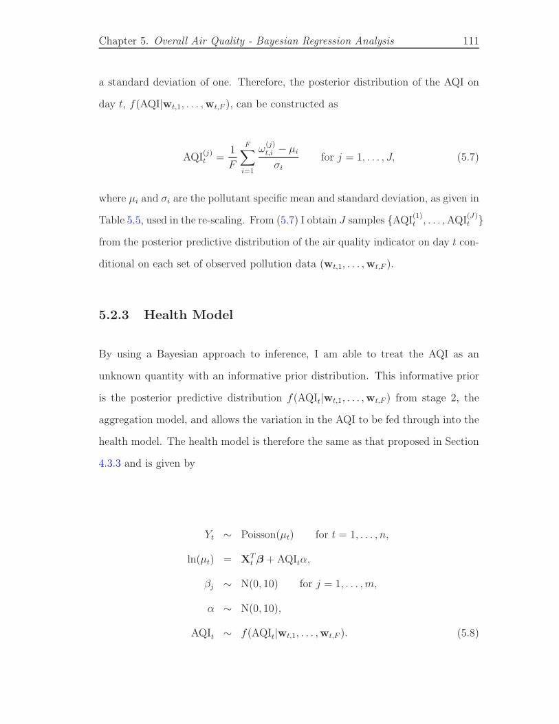
Chapter 5. Overall Air Quality - Bayesian Regression Analysis 111
a standard deviation of one. Therefore, the posterior distribution of the AQI on
day t, f(AQI|wt,1, . . . ,wt,F ), can be constructed as
AQI(j)t =
1
F
F∑
i=1
ω(j)t,i − µi
σifor j = 1, . . . , J, (5.7)
where µi and σi are the pollutant specific mean and standard deviation, as given in
Table 5.5, used in the re-scaling. From (5.7) I obtain J samples AQI(1)t , . . . ,AQI
(J)t
from the posterior predictive distribution of the air quality indicator on day t con-
ditional on each set of observed pollution data (wt,1, . . . ,wt,F ).
5.2.3 Health Model
By using a Bayesian approach to inference, I am able to treat the AQI as an
unknown quantity with an informative prior distribution. This informative prior
is the posterior predictive distribution f(AQIt|wt,1, . . . ,wt,F ) from stage 2, the
aggregation model, and allows the variation in the AQI to be fed through into the
health model. The health model is therefore the same as that proposed in Section
4.3.3 and is given by
Yt ∼ Poisson(µt) for t = 1, . . . , n,
ln(µt) = XTt β + AQItα,
βj ∼ N(0, 10) for j = 1, . . . , m,
α ∼ N(0, 10),
AQIt ∼ f(AQIt|wt,1, . . . ,wt,F ). (5.8)

Chapter 5. Overall Air Quality - Bayesian Regression Analysis 112
The regression parameters (β1, . . . , βp, α) are assigned diffuse Gaussian priors, with
a mean of zero and a variance of 10. Inference is based on MCMC methods, where
the parameters are updated in three batches, namely, β = (β1, . . . , βp), α and
AQItnt=1. Both the covariate regression parameters β and the pollution-health
relationship α are updated via Metropolis steps, using random walk proposal dis-
tributions. The AQI on day t is updated by randomly selecting one of the J
samples AQI(1)t , . . . ,AQI
(J)t from f(AQIt|wt,1, . . . ,wt,F ), its posterior predictive
distribution, thus correctly allowing for the uncertainty in its value.
5.3 Model Validation
As a preliminary means of assessing the predictive accuracy of (5.1), and also to
provide a means of comparing both the model proposed here and that of (4.4)
from Chapter 4, I used the method of cross validation, which was previously de-
scribed in Section 2.6.2. I applied the method of cross validation to the PM10
data from Greater London for the time period 2001 to 2003. However, only sites
which recorded concentrations for 75% of the time period were included. Both
of these models aim to create a spatially representative measure of pollution by
smoothing over the available data. I thus deliberately choose PM10 for the pur-
poses of cross-validation as these data are known to be spatially heterogeneous
(Peng and Bell (2010)). A model which can therefore capture this aspect of the
data and adequately predict these concentrations should not be over smoothing
any subsequent predictions at new locations. To create a training set of data a
number of sites have to be removed from the original data set. Of the 49 sites
which measured PM10 approximately 60% were located at the roadside (Table 5.2),
therefore, to create a training set which is made up of 90% of the monitoring sites

Chapter 5. Overall Air Quality - Bayesian Regression Analysis 113
(44 sites), 11% (3 sites) and 10% (2 sites) of the roadside and background sites
were removed respectively. The data which relate to the removed sites are used
as the validation data set. The regression model (5.1) proposed in this chapter
and the geostatistical model (4.4), proposed in the previous chapter, were applied
to the training data. The regression model was applied to the data from all days
simultaneously, while the geostatistical model was applied separately for each day.
A regression model with no time-varying coefficient was also applied, to determine
if this added complexity was necessary, in terms of the model’s predictive capa-
bilities. To determine the accuracy of the predictions made by each of the three
models, the median posterior predictive distribution for each of the removed sites
is compared to that locations observed PM10 level. This was done by calculating
the prediction bias (PB, (2.17)) and the median absolute deviation (MAD, (2.18)).
This method was carried out a total of 5 times, to assess the variability of the re-
sults to the 10% of sites removed. The five validation (red) and training (black)
data sets are given in Figure 5.1. The choice of creating five scenarios of test and
validation data is a somewhat arbitrary one, however, the use of cross-validation
to assess the predictive accuracy and facilitate the comparison of models is only
meant as a small preliminary method in order to get a feel for which model, if
either, outperforms the other.
5.3.1 Results
I assessed the predictive accuracy of both the regression model (5.1) and the geosta-
tistical model (4.4). The results for each of the 5 validation data sets are presented
in Table 5.1, which displays the prediction bias and median absolute deviation,
both of which are given relative to the observed concentrations of PM10, which

Chapter 5. Overall Air Quality - Bayesian Regression Analysis 114
510 520 530 540 550 560
160
170
180
190
200
(a)
Easting
Nor
thin
g
510 520 530 540 550 560
160
170
180
190
200
(b)
Easting
Nor
thin
g
510 520 530 540 550 560
160
170
180
190
200
(c)
Easting
Nor
thin
g
510 520 530 540 550 560
160
170
180
190
200
(d)
Easting
Nor
thin
g
510 520 530 540 550 560
160
170
180
190
200
(e)
Easting
Nor
thin
g
Figure 5.1: Locations of the training (black) and validation (red) PM10 mon-itoring sites within Greater London, used in each of the 5 (a - e) test cases (•,
roadside locations; , background locations).

Chapter 5. Overall Air Quality - Bayesian Regression Analysis 115
have a mean value of 24.783 (Table 5.2). In addition, an overall average across
the five validation data sets has been given for each model and each summary.
To determine if the inclusion of a time-varying coefficient improves the predictive
capabilities of the model, I have also applied the cross validation to a Bayesian
regression model which does not include a time-varying coefficient.
Table 5.1: The PB and MAD scores, relative to observed PM10, for the re-gression model (5.1), without and with a time-varying coefficient, and the geo-
statistical model, presented in Chapter 4.
Regression Model
Scenario Non time-varying model Time-varying model Geostatistical modelPB MAD PB MAD PB MAD
1 2.786 7.019 2.773 7.021 -1.062 3.2662 2.332 6.329 2.339 6.344 -0.651 2.6773 -2.294 7.316 -2.381 7.367 -6.468 6.6264 1.700 6.402 1.680 6.365 -1.499 3.2195 1.738 6.587 1.714 6.562 -1.456 4.134
Average 1.252 6.731 1.225 6.732 -2.227 3.984
Under each regression model, both without and with a time-varying coefficient,
the differences between the median absolute deviation for each set of validation
data is small, having a range of approximately 1µgm−3 in each case. The predic-
tion bias, however, does change between sets and in particular is negative (-2.294
and -2.381) for test set three, compared to the positive, and hence over prediction,
for all the other test data sets. This may be due to the three roadside mon-
itors which were removed being all located within the center of London where
PM10 levels will be particularly high (Figure 5.1(c)), hence the models are under
predicting these sites based on the remaining data. Between the two regression
models there is very little difference in the prediction bias and median absolute
deviation results for each validation data set. This suggest that the time-varying
Chapter 5. Overall Air Quality - Bayesian Regression Analysis 116
coefficient is having little effect on the predictive capabilities of the model. Under
the geostatistical model both the prediction bias and median absolute deviation
are different for test set 3, compared to the other test sets. However, under this
approach this has resulted in a larger negative prediction bias compared to the al-
ready negative results of the other test sets and a larger median absolute deviation.
Over the 5 test cases the geostatistical model has outperformed both the regression
models in terms of the average amount of error between the observed concentra-
tions and the predictions as measured by the average median absolute deviation,
which is approximately one and a half times smaller than the same result for each
regression model. In terms of the overall bias in the predictions the geostatistical
model consistently under estimates the true concentrations levels and therefore
has a overall average prediction bias of -2.227. This is compared to the regression
models which overestimate the true concentrations, except in the case of validation
data set 3, and therefore the overall average prediction bias is positive at 1.252
for the model with no time-varying coefficient and 1.225 for the model with such
a coefficient.
The results of the model validation suggests that overall the geostatistical model,
proposed in Chapter 4, is outperforming the simple regression model, both without
and with a time-varying coefficient, which was proposed here as an alternative
method. Excluding the results from validation data set 3, the absolute overall
prediction bias under each regression model is larger (2.139 and 2.127), than that
of the geostatistical model (-1.167). In addition to this, the predictions from the
regression model appear to be very sensitive as to which monitor observations are
included in the model. If sites which record very high concentrations are included

Chapter 5. Overall Air Quality - Bayesian Regression Analysis 117
then the model tends to over predict the true concentrations. This bias in the
pollution estimate could result in a bias in the associated health risks. While the
results do suggest that the geostatistical model is more favourable, it should be
noted that both the prediction bias and the median absolute deviation under both
models are comparatively small compared to the average PM10 concentrations for
the same time period.
5.4 Application - Greater London
5.4.1 Description of Data
The methods developed in this chapter use the air pollution and health data for
the city of Greater London, England, for the period 2001 to 2003. This is the
same data set which was previously described in Section (4.4).
5.4.1.1 Pollution Data
The pollution concentrations used in this chapter are the same as those which were
described in Section 4.4.1.1 previously. However, as there were large amounts of
missing data for each pollutant (Table 4.1) only sites which had at least 75% of the
data were included in the analysis in this chapter, as opposed to that in Chapter
4 which included all sites. Thus allowing days with missing data to be excluded
from the analysis without eliminating the majority of the data. Thus for each of
the four pollutants the number of sites were reduced to give 25 sites for CO, 67 for
NO2, 23 for O3 and 49 for PM10. The four pollutants are summarised in Figure
5.2 and Table 5.2, which respectively display the locations of the monitoring sites

Chapter 5. Overall Air Quality - Bayesian Regression Analysis 118
510 520 530 540 550 560
160
170
180
190
200
(a)
Easting
Nor
thin
g
510 520 530 540 550 560
160
170
180
190
200
(b)
Easting
Nor
thin
g
510 520 530 540 550 560
160
170
180
190
200
(c)
Easting
Nor
thin
g
510 520 530 540 550 560
160
170
180
190
200
(d)
Easting
Nor
thin
g
510 520 530 540 550 560
160
170
180
190
200
(e)
Easting
Nor
thin
g
Figure 5.2: Location and type of the pollution monitors in Greater London(•, roadside locations; , background locations): (a) CO, (b) NO2, (c) O3, (d)
PM10, and (e) the prediction locations.

Chapter 5. Overall Air Quality - Bayesian Regression Analysis 119
and summary statistics. The figure and table show that NO2 is still measured at
the largest number of sites across the city (67 sites) and therefore provides the
best spatial coverage of Greater London. In contrast O3 and CO are monitored
at the fewest sites, 23 and 25 respectively, and therefore do not cover the study
region particularly well. Between approximately 54% and 60% of the monitors for
CO, NO2 and PM10 are located at roadside environments, where concentration
levels are likely to be considerably higher. However, only approximately 32% of
the monitors for O3 are placed at the roadside.
The amount of spatial variation in each pollutant’s concentrations over the three-
year study period, which is represented as a coefficient of variation (CoV, spatial
standard deviation divided by the mean) are displayed in Table 5.2. The amount
of spatial variation is smallest for O3 (CoV = 0.287), which is likely to be because
unlike the other pollutants, its concentration is not driven driven by local traffic
sources. Conversely, it is largest for CO (CoV = 0.612), the source of which is
almost entirely traffic related.
As described in Section 4.4.1.1, the modelled yearly average concentrations of CO,
NO2 and PM10 are available at 1 kilometer intervals across London. These data
are displayed in Figure 4.2 where it can be seen that the highest concentrations
occur in the city centre and decrease as you move further out. The exception is
London Heathrow airport, which is situated in the west of London, where con-
centrations are also very high. These modelled concentrations form the covariate
which is fixed in time but I wish its effect to be variable in time. Again there is
no such data available for O3, which means that only a regression model without
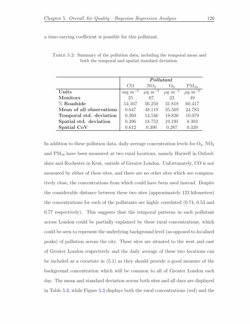
Chapter 5. Overall Air Quality - Bayesian Regression Analysis 120
a time-varying coefficient is possible for this pollutant.
Table 5.2: Summary of the pollution data, including the temporal mean andboth the temporal and spatial standard deviation.
Pollutant
CO NO2 O3 PM10
Units mg m−3 µg m−3 µg m−3 µg m−3
Monitors 25 67 23 49% Roadside 54.167 56.250 31.818 60.417Mean of all observations 0.647 48.119 35.569 24.783Temporal std. deviation 0.260 14.546 18.826 10.079Spatial std. deviation 0.396 18.752 10.191 8.393Spatial CoV 0.612 0.390 0.287 0.339
In addition to these pollution data, daily average concentration levels for O3, NO2
and PM10 have been measured at two rural locations, namely Harwell in Oxford-
shire and Rochester in Kent, outside of Greater London. Unfortunately, CO is not
measured by either of these sites, and there are no other sites which are compara-
tively close, the concentrations from which could have been used instead. Despite
the considerable distance between these two sites (approximately 123 kilometres)
the concentrations for each of the pollutants are highly correlated (0.74, 0.53 and
0.77 respectively). This suggests that the temporal patterns in each pollutant
across London could be partially explained by these rural concentrations, which
could be seen to represent the underlying background level (as opposed to localised
peaks) of pollution across the city. These sites are situated to the west and east
of Greater London respectively and the daily average of these two locations can
be included as a covariate in (5.1) as they should provide a good measure of the
background concentration which will be common to all of Greater London each
day. The mean and standard deviation across both sites and all days are displayed
in Table 5.3, while Figure 5.3 displays both the rural concentrations (red) and the

Chapter 5. Overall Air Quality - Bayesian Regression Analysis 121
observed monitor average (black) for each of the three pollutants for each day of
the three year study period. The rural concentrations follow the same temporal
patterns as the observed concentrations and with the exception of O3 are lower
than the observed concentrations. As mentioned previously ozone is not affected
by traffic emissions but is instead formed as part of a reaction in the atmosphere,
the trigger for which is sunlight. It is therefore not unexpected that ozone con-
centrations would be slightly higher outside the city where sunlight is not blocked
by tall buildings.
5.4.1.2 Meteorological data
The London Air Quality Network (LAQN) records data about a number of meteo-
rological variables, including barometric pressure, relative humidity, solar radiation
and temperature. As mentioned previously temperature is known to play a role
in the collection of air borne particles, such as pollutants, in the atmosphere. A
number of other meteorological variables also play a prominent part. For example
the creation of ozone in the atmosphere is triggered by sunlight, which suggests
that solar radiation may explain the observed concentrations of this pollutant.
The meteorological variables, summarised in Table 5.3, can therefore be included
in (5.1) as possible explanatory variables. Temperature is recorded at the largest
number of sites (16), and over the 3 year period of the study the average tempera-
ture was 12.876C. Barometric pressure measures the force exerted onto ourselves
and the objects around us by the weight of the air above. The average value of
1011.356mBar is fairly typically of what is seen in the UK on a day to day ba-
sis. The amount of water vapor in the air is measured by the relative humidity,
which for the UK is typically between 50 and 85%, the average value for the study
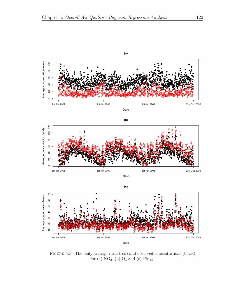
Chapter 5. Overall Air Quality - Bayesian Regression Analysis 122
020
4060
8010
0
(a)
Date
Ave
rage
con
cent
ratio
n le
vels
1st Jan 2001 1st Jan 2002 1st Jan 2003 31st Dec 2003
020
4060
8010
012
0
(b)
Date
Ave
rage
con
cent
ratio
n le
vels
1st Jan 2001 1st Jan 2002 1st Jan 2003 31st Dec 2003
1020
3040
5060
70
(c)
Date
Ave
rage
con
cent
ratio
n le
vels
1st Jan 2001 1st Jan 2002 1st Jan 2003 31st Dec 2003
Figure 5.3: The daily average rural (red) and observed concentrations (black)for (a) NO2, (b) O3 and (c) PM10.

Chapter 5. Overall Air Quality - Bayesian Regression Analysis 123
Table 5.3: Summary of the daily rural pollution concentrations and the me-teorological data, available for Greater London in the period 2001 to 2003.
Data Units Monitors Mean Std. Deviation
Rural NO2 concentrations µgm−3 2 18.837 10.813
Rural O3 concentrations µgm−3 2 51.799 20.279Rural PM10 concentrations µgm−3 2 20.245 9.405
Barometric pressure mBar 5 1011.356 10.354Relative humidity % 2 75.026 8.770Solar radiation W/m2 3 100.180 73.119Temperature C 16 12.876 5.580
period of 75.026% is therefore standard. Finally, solar radiation is the total fre-
quency spectrum of electromagnetic radiation produced by the sun. In the North
of Britain this is typically around 85 W/m2, however, in the South the amount of
solar radiation is often seen to be as high as 110 W/m2. Therefore, the average
solar radiation in Greater London of 100.180 W/m2, for the period 2001 to 2003,
is typical as Greater London is situated in the South of the UK.
5.4.2 Statistical Modelling
5.4.2.1 Pollution Modelling
For each of the four pollutants, CO, NO2, O3 and PM10, a linear model was used to
determine which covariates should be included in (5.1). The daily measurements of
meteorology and the average rural concentrations, summarised in Table 5.3, were
considered along with indicator variables for day of the week or weekend and a
smooth function of time. Initially, I examined the relationship between each of the
possible covariates (via pairwise comparison plots) and determined which, if any,
were highly correlated. I then fitted a model which included all covariates which

Chapter 5. Overall Air Quality - Bayesian Regression Analysis 124
were not highly correlated. If any pair of covariates appeared to be particularly
correlated then I included just one of the variables initially. I refined my covariate
selection by excluding any variable which did not have a significant p-value. In the
case of highly correlated variables I considered each in turn, if they all had signif-
icant p-values then I only included the one which most reduced the models AIC. I
also decided to include a natural cubic spline of time, as several of the pollutants,
NO2 in particular, exhibited a clear temporal pattern. For each pollutant I chose
the number of knots to be included by considering the autocorrelation function
of the residuals and also which value corresponded to the lowest AIC. For each
pollutant the number of knots considered ranged between 3 and 6 per year. The
yearly average modelled concentrations were also included, however the effect of
these yearly estimates were allowed to vary over time, via the second order ran-
dom walk which was proposed for their associated coefficient. No such values are
available for ozone therefore this pollutant can only be modelled as a regression
model which does not include a time-varying coefficient. All pollution concentra-
tions, namely the original pollution data, the rural concentrations and the yearly
average estimates were modelled on the log scale, as they are non-negative and
exhibit right skew.
The priors used in each regression model were those described in Section 5.2, and
include an improper prior (U(−∞,∞)) for the coefficients of the non time-varying
variables and an improper reciprocal prior for the variances σ2 and τ 2 i.e. 1/σ2 and
1/τ 2 respectively. The coefficients of the time-varying covariates were assigned a
second-order random walk, as this will allow for a reasonably smooth function over
time. The starting values (δ0, δ1) were also assigned improper priors (U(−∞,∞)).

Chapter 5. Overall Air Quality - Bayesian Regression Analysis 125
Inference for (5.1) was implemented using MCMC methods and in particular Gibbs
sampling. Inference was based on J = 20, 000 samples from the joint posterior
distribution of the model, less a period of 5,000 samples which were removed for
burn-in. For each pollutant the logged concentrations of pollution were predicted
on a regular grid at 2 kilometre intervals across Greater London, corresponding
to 399 sites in total. All prediction locations are considered background rather
than roadside locations, because they are likely to be more representative of the
pollution concentrations to which the population are exposed. For each of the
15, 000 samples the predictions were exponentiated, weighted by the population
density and subsequently averaged, thus giving 15, 000 samples from the posterior
predictive distribution of (4.3). Finally, to create the posterior predictive distri-
bution for the air quality indicator, the 15, 000 posterior predictive samples from
(4.3) for each pollutant were combined using (5.7).
5.4.2.2 Health Modelling
The health model proposed in this chapter is the same as that which was proposed
in Chapter 4, therefore only a brief description will be given here. In addition to the
measure of pollution, the covariates in the health model also include the mean daily
temperature and smooth function of time, both of which were included to capture
the prominent seasonal pattern in the daily mortality series which was seen in
Figure 4.3(a). A quadratic relationship was specified for the relationship between
temperature and respiratory related deaths, as a slight “U” shaped relationship can
be observed between the two variables (4.3(c)). The remainder of the prominent
seasonal pattern in the mortality data is represented by a natural cubic spline of
time (day of the study), with seven degrees-of-freedom per year. Finally, I added a
measure of air pollution to the model at a lag of one day, because previous studies,

Chapter 5. Overall Air Quality - Bayesian Regression Analysis 126
such as those by Dominici et al. (2000), Zhu et al. (2003) and Lee and Shaddick
(2008), have shown that exposure to air pollution is unlikely to result in health
effects on the same day.
5.4.3 Results
5.4.3.1 Pollution Model Results
The main results of interest from the regression model, both with and without the
inclusion of a time-varying coefficient, are the posterior predictive distributions of
(4.3) for the individual pollutants on each of the 1095 days of the study, as well
as the corresponding distributions for the aggregation of the concentration levels
as given by (5.7). For a sample month of July, a summary of these distributions is
presented in Figures 5.4 and 5.7, for the model without and with a time-varying
coefficient respectively. A corresponding plot for all 1095 days is not included as
it looked overly cluttered. Each posterior predictive distribution is summarised
by its posterior median (black dots) and a 95% credible intervals (vertical lines),
while for the purposes of comparison the monitor average, as given by (3.2), has
also been included as the solid black line. In addition to this, a temporal summary
of the posterior predictive distributions, in terms of the mean and standard devi-
ation, are given in Tables 5.4 and 5.5, for each of the four pollutants, CO, NO2,
O3, and PM10 and the AQI.
Regression Model with no time-varying coefficient

Chapter 5. Overall Air Quality - Bayesian Regression Analysis 127
0.2
0.4
0.6
0.8
1.0
(a)C
O
1st July 2001 15th July 2001 31st July 2001
1020
3040
5060
7080
(b)
NO
2
1st July 2001 15th July 2001 31st July 2001
2040
6080
100
120
(c)
O3
1st July 2001 15th July 2001 31st July 2001
1020
3040
50
(d)
PM
10
1st July 2001 15th July 2001 31st July 2001
−1
01
2
(e)
AQ
I
1st July 2001 15th July 2001 31st July 20011st July 2001 15th July 2001 31st July 2001
Figure 5.4: Posterior medians (•) and 95% credible intervals ( | ) from theregression model without a time-varying coefficient and the monitor average forthe individual pollutants (a) CO, (b) NO2, (c) O3, (d) PM10 and (e) the air
quality indicator (AQI).

Chapter 5. Overall Air Quality - Bayesian Regression Analysis 128
Firstly, to ensure that the Markov chain Monte Carlo simulations had converged
diagnostic plots of the coefficients were examined. As there are too many coeffi-
cients to show for each pollutant the resulting plots for just the variance parameter,
σ2, is shown for each of the four pollutants, CO, NO2, O3 and PM10 (Figure 5.5).
From this plot we can see that the variance parameter has converged.
Figure 5.4 shows that for the month of July, 2001, the monitor average of CO
is considerably higher than the posterior median of (4.3), which is likely to be
because the latter adjusts for preferential sampling and is based on predictions
at background locations. The posterior medians for NO2 and PM10, are very
similar to the monitor average with the exception of when the concentrations are
particularly high (approximately 25µg m−3 and 50µg m−3 respectively), in which
case the posterior median is visibly less than the monitor average. This may again
be because predictions are based at background locations where concentrations
are likely to be lower. For O3 the posterior median and monitor average are very
similar with the posterior being marginally higher for the month of July, 2001. This
is likely to be because ozone is not affected by traffic emissions. The uncertainty
intervals for all of the pollutants are very small. These small uncertainty intervals
are likely to be due to a small variance, σ2, and regression coefficients, β, that
exhibit very little posterior uncertainty. For each of the four pollutants CO, NO2,
O3 and PM10 the variance, σ2, is small at only 0.346, 0.113, 0.202 and 0.098
respectively for each pollutant. There is also little variability in the estimates of
the regression coefficients, as the largest inter quartile range, over all coefficients for
each pollutant, is 0.007. This lack of posterior uncertainty is likely to be because
all the available data is used in each model. Both in terms of the temporal pattern
in the posterior medians and the width of the credible intervals, the values for the

Chapter 5. Overall Air Quality - Bayesian Regression Analysis 129
0.33
00.
340
0.35
0(a)
Simulations
σ2
5000 10000 15000 20000
0.11
00.
112
0.11
4
(b)
Simulations
σ2
5000 10000 15000 20000
0.19
50.
205
(c)
Simulations
σ2
5000 10000 15000 20000
0.09
60.
098
0.10
0
(d)
Simulations
σ2
5000 10000 15000 20000
Figure 5.5: The results of the 20,000 MCMC simulations for the varianceparameter σ
2, less the burn-in period, proposed by the regression model withouta time-varying coefficient.

Chapter 5. Overall Air Quality - Bayesian Regression Analysis 130
AQI shown in Figure 5.4(e) are an amalgamation of the four individual pollutants.
Table 5.4: Summary of the posterior predictive distributions found when im-plementing the regression model with no time-varying coefficient.
Pollutant
CO NO2 O3 PM10 AQIUnits mg m−3 µg m−3 µg m−3 µg m−3 -Temporal mean 0.444 44.094 37.940 21.539 0.111Temporal std. deviation 0.128 13.292 20.004 7.980 0.514
As only a single month is presented in Figure 5.4 an overall summary of the daily
posterior predictive distributions are given in Table 5.4. For CO, NO2 and PM10
the average daily mean and standard deviation from the posterior predictive dis-
tributions are lower than that of the observed data (Table 5.2). However, the
equivalent values for ozone are higher than the observed data.
Regression Model with Time-varying Coefficient
Firstly, to ensure that the Markov chain Monte Carlo simulations had converged
diagnostic plots of the coefficients were examined. As there are too many coeffi-
cients to show for each pollutant the resulting plots for just the variance parameter,
σ2, is shown for each of the three pollutants, CO, NO2, and PM10 (Figure 5.5).
From this plot we can see that the variance parameter has converged.
The pollution model results for the regression model which included a time-varying
coefficient for the modelled pollution estimates are similar to those found under
the same model which did no include a time-varying coefficient. The results are
displayed in Figure 5.7 and Table 5.5. The monitor average of CO is considerably
higher than the posterior median of (4.3), for the month of July 2001. This is also

Chapter 5. Overall Air Quality - Bayesian Regression Analysis 131
0.33
50.
340
0.34
50.
350
(a)
Simulations
σ2
5000 10000 15000 20000
0.10
80.
109
0.11
00.
111
0.11
2
(b)
Simulations
σ2
5000 10000 15000 20000
0.09
60.
097
0.09
80.
099
0.10
0
(c)
Simulations
σ2
5000 10000 15000 20000
Figure 5.6: The results of the 20,000 MCMC simulations for the varianceparameter σ
2, less the burn-in period, proposed by the regression model with atime-varying coefficient.

Chapter 5. Overall Air Quality - Bayesian Regression Analysis 132
0.2
0.4
0.6
0.8
1.0
(a)C
O
1st July 2001 15th July 2001 31st July 2001
1020
3040
5060
7080
(b)
NO
2
1st July 2001 15th July 2001 31st July 2001
1020
3040
50
(c)
PM
10
1st July 2001 15th July 2001 31st July 2001
−1
01
2
(d)
AQ
I
1st July 2001 15th July 2001 31st July 2001
Figure 5.7: Posterior medians (•) and 95% credible intervals ( | ) from theregression model with a time-varying coefficient and the monitor average forthe individual pollutants (a) CO, (b) NO2, (c) PM10, and (d) the air quality
indicator (AQI).

Chapter 5. Overall Air Quality - Bayesian Regression Analysis 133
true for NO2 and PM10 although to a lesser extent. The 95% credible intervals
are largest for CO, although they are comparatively small for all three individual
pollutants. As in the case of the regression model with no varying coefficient,
the lack of uncertainty intervals may be explained by small estimates of the vari-
ance, σ2, and/or estimates of β which do not vary very much. As this model
also includes a time-varying coefficient, represented by δ, the small uncertainty
intervals may also be due to this coefficient being equal to zero or not varying.
For each of the three pollutants, CO, NO2 and PM10, the median (and associated
95% uncertainty interval) for δ, after excluding a burn-in period of 5000 samples,
are 0.259 (0.225, 0.300), 0.019 (0.016, 0.022) and 0.046 (0.037, 0.053) respectively.
For both NO2 and PM10, δ is therefore very close to zero. For each pollutant
the range of possible values for δ is very small, this would suggest that it was
not necessary to include a time-varying coefficient. Both in terms of the tem-
poral pattern in the posterior medians and the width of the credible intervals,
the values for the AQI shown in Figure 5.7(e) are an amalgamation of the four
individual pollutants. These results may suggest that concentrations of each pol-
lutant, including the AQI, are not varying greatly from day-to-day, and that the
resulting posterior predictive distributions are overly smooth. If this is the case
then associated health risks, which are estimated in Section 5.4.3.2, may be biased.
Table 5.5: Summary of the posterior predictive distributions found whenimplementing the regression model with a time-varying coefficient.
Pollutant
CO NO2 PM10 AQIUnits mg m−3 µg m−3 µg m−3 µg m−3 -Temporal mean 0.444 38.9112 21.541 -0.0007Temporal std. deviation 0.128 11.672 7.999 0.700

Chapter 5. Overall Air Quality - Bayesian Regression Analysis 134
An overall summary of the daily posterior predictive distributions for the three
individual pollutants, CO, NO2 and PM10, and the AQI, are given in Table 5.5.
The average daily mean and standard deviation of the posterior predictive distri-
bution is less than that of the observed concentrations for each pollutant. This is
likely to be because the posterior predictive distributions are based on predictions
at background locations and each of CO, NO2 and PM10 are driven in part by
traffic emissions.
5.4.3.2 Health Model Results
I estimated the health effects of the four individual pollutants as well as overall air
quality, the latter of which was represented by the air quality indicator given by
(5.7). In each case I applied the standard modelling approach, which is to include a
single representative value of air pollution given by the monitor average in a health
model such as (4.1), and the Bayesian hierarchical model proposed in this chapter.
This will allow me to observe the differences between the two approaches. The
results are presented in Table 5.6, which displays the relative risks and associated
95% uncertainty intervals for the effects of each pollutant on health. The relative
risks, in each case, relate to an increase of one temporal standard deviation of the
posterior predictive distribution (as given in Table 5.5) in each pollutants values.
The results suggest that only overall air quality, as measured by the monitor aver-
age air quality index, has substantial health risks, as the 95% uncertainty interval
is entirely positive. Each of the individual pollutants does not exhibit substantial
health risks on their own as their associated 95% uncertainty intervals do contain
the null risk of one.
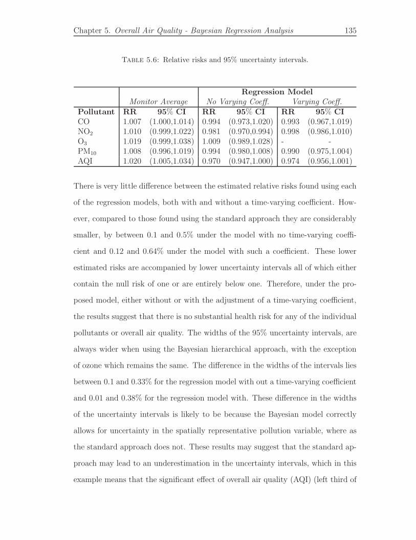
Chapter 5. Overall Air Quality - Bayesian Regression Analysis 135
Table 5.6: Relative risks and 95% uncertainty intervals.
Regression ModelMonitor Average No Varying Coeff. Varying Coeff.
Pollutant RR 95% CI RR 95% CI RR 95% CICO 1.007 (1.000,1.014) 0.994 (0.973,1.020) 0.993 (0.967,1.019)NO2 1.010 (0.999,1.022) 0.981 (0.970,0.994) 0.998 (0.986,1.010)O3 1.019 (0.999,1.038) 1.009 (0.989,1.028) - -PM10 1.008 (0.996,1.019) 0.994 (0.980,1.008) 0.990 (0.975,1.004)AQI 1.020 (1.005,1.034) 0.970 (0.947,1.000) 0.974 (0.956,1.001)
There is very little difference between the estimated relative risks found using each
of the regression models, both with and without a time-varying coefficient. How-
ever, compared to those found using the standard approach they are considerably
smaller, by between 0.1 and 0.5% under the model with no time-varying coeffi-
cient and 0.12 and 0.64% under the model with such a coefficient. These lower
estimated risks are accompanied by lower uncertainty intervals all of which either
contain the null risk of one or are entirely below one. Therefore, under the pro-
posed model, either without or with the adjustment of a time-varying coefficient,
the results suggest that there is no substantial health risk for any of the individual
pollutants or overall air quality. The widths of the 95% uncertainty intervals, are
always wider when using the Bayesian hierarchical approach, with the exception
of ozone which remains the same. The difference in the widths of the intervals lies
between 0.1 and 0.33% for the regression model with out a time-varying coefficient
and 0.01 and 0.38% for the regression model with. These difference in the widths
of the uncertainty intervals is likely to be because the Bayesian model correctly
allows for uncertainty in the spatially representative pollution variable, where as
the standard approach does not. These results may suggest that the standard ap-
proach may lead to an underestimation in the uncertainty intervals, which in this
example means that the significant effect of overall air quality (AQI) (left third of

Chapter 5. Overall Air Quality - Bayesian Regression Analysis 136
Table 5.6) could actually be non-significant (centre and right thirds of Table 5.6).
5.5 Discussion
In this chapter I have presented a statistical approach for constructing a spa-
tially representative measure of overall air quality and estimating its effects on
health, whilst taking proper account of the uncertainty in the estimate. The pro-
posed approach is to model the concentrations for a single pollutant over space
and time simultaneously using a Bayesian regression model which incorporates
available covariate information, such as measures of meteorology, to describe the
spatio-temporal pattern in the pollution concentrations. This approach is compu-
tationally simpler than that which was proposed in Chapter 4, for also meeting
such aims. The model proposed in this chapter should also be able to produce
more precise estimates of the unknown parameters because data from all days are
used in the estimation. To increase the flexibility of the model I also included a
time-varying coefficient, as this will allow the effects of any covariate which is fixed
in time to vary over time. The motivation for the inclusion of such a coefficient
are the 1 kilometre estimates for the pollutants CO, NO2 and PM10, which are
available for the year 2001.
A preliminary assessment of the predictive accuracy of both the geostatistical
model proposed in Chapter 4 and the regression model proposed here, both with-
out and with the inclusion of a time-varying coefficient, are compared via the
method of cross-validation. A total of 5 test cases (scenarios) were constructed,
each of which was made up of a training data set which contained 90% (44 sets)
of the total number of sites (49 sites) and a validation data set which was made

Chapter 5. Overall Air Quality - Bayesian Regression Analysis 137
up of the remaining 10% of the sites. The results, which are displayed as the
prediction bias and the median absolute deviation for each test case, suggest that
the simple regression model tends to over predict the true concentration value.
Conversely, the geostatistical model tends to show bias towards under predicting
the true concentrations. Over the 4 scenarios (excluding scenario 3 which pro-
duced noticeably different results) for the cross-validation, the absolute overall
prediction bias and median absolute deviation were larger under each of the re-
gression models compared to the equivalent results under that of the geostatistical
model. In scenario 3, three roadside sites all of which were located in the centre
of London were randomly removed. This resulted in both regression models under
predicting the true concentrations. This would suggest that the simple regression
model is highly sensitive to which monitoring site data is included in the model.
When data are not independent the method of cross-validation can be problematic
as leaving out an observation will not remove all the associated information due
to the correlations with the other observations, a problem frequently seen in the
use of cross-validation in time series studies. Given that the concentrations of
neighboring sites are undoubtedly going to be highly correlated this method may
have been a poor choice even for the purposes of obtaining a simple comparison
of two modelling approaches. Further to this, I only considered the results from 5
scenarios. This small number of test cases may not have yielded reliable results,
for example the results of scenario 3 may in fact be what should be expected from
the proposed models.
The regression modelling of CO, NO2 and PM10 produced areal-level pollution
estimates that were generally lower than the corresponding monitor average. One

Chapter 5. Overall Air Quality - Bayesian Regression Analysis 138
of the reasons for this difference is that the regression model adjusted for the dif-
ferences in the pollution concentrations at roadside and background environments,
an aspect which is typically ignored in the majority of studies. However, the same
areal-level pollution estimates for O3 were generally higher than the correspond-
ing monitor average. This may be because ozone is not attributable to traffic
emissions and is instead produced by the collision of oxygen and oxides in the
atmosphere. The other main difference between the standard modelling approach
and the Bayesian regression model proposed here concerns the treatment of un-
certainty in the areal-level pollution estimate. The standard modelling approach
typically ignores the uncertainty in the monitor average when estimating its health
effects, while the approach proposed here correctly feeds through the variation in
the pollutants posterior predictive distribution into the health model. This prop-
agation of uncertainty through the hierarchical model results in wider uncertainty
intervals compared with the standard approach, which in the London example re-
sulted in the change in the significance of the health risks of the AQI. Under the
approach proposed in this chapter none of the individual pollutants or the measure
of overall air quality has a substantial effect on human health. The conclusion that
the individual pollutants and overall air quality do not pose and any significant
risks to health under the proposed model is somewhat unusual. In the current
literature there are many studies which investigate the health risks of numerous
individual pollutants and while they may not all produce significant results many
do. For example particulate matter is consistently found to be detrimental to hu-
man health (see for example Laden et al. (2000) and Diaz et al. (2012)). However,
as expressed in Chapter 4 these results are contingent on many modelling decisions
including the choice of lag and aggregation methods. As discussed previously the
some of the modelling choices made in this thesis, including the decision to ignore

Chapter 5. Overall Air Quality - Bayesian Regression Analysis 139
overdispersion, may not have been prudent and may have affected the outcome of
the proposed modelling methods.
The Bayesian regression model was proposed as an alternative to the computa-
tionally expensive geostatistical method proposed in the previous chapter. This
method also met the aims of producing a spatially representative measure of over-
all air quality which can be incorporated into a health model while taking proper
account of the uncertainty in the estimate. The results of the cross-validation
suggest this model is being outperformed by the geostatistical model and that it
is very sensitive to the data which are included. To fully assess the abilities of this
model a simulation study could be carried out. These results and also those from
the pollution modelling which was applied to all four pollutants suggested that the
inclusion of a time-varying coefficient was not worth while. This added complexity
made no difference to the predictive capabilities of the model and the resulting
estimates of δ were small and did not vary very much over the time period.

Chapter 6
Estimating Constrained
Concentration-Response
Functions
6.1 Introduction
As discussed previously in Section 3.2.2, the majority of studies estimate a linear
Concentration-Response Function (CRF) between ambient air pollution levels and
a health outcome (for example Dominici et al. (2000) and Carder et al. (2008)).
This is because the resulting CRF can be summarized by a single regression coeffi-
cient. However, a number of studies have relaxed this constraint, which has allowed
them to examine whether the CRF exhibits any non-linear behavior (see for exam-
ple Schwartz (2001) and Dominici et al. (2002)). The majority of such non-linear
concentration-response functions have been modelled using cubic splines, which
restrict the estimated curves to be smooth (three times differentiable), but do not
140

Chapter 6. Estimating Constrained Concentration-Response Functions 141
enforce any constraints on their shape. This lack of shape constraints has resulted
in unfeasible CRFs being estimated, such as those that exhibit decreasing health
effects as the ambient concentrations increase. Examples of this phenomenon in-
clude Figure 6.6 panel (b) in this chapter and Figure 3 in Schwartz et al. (2001),
both of which exhibit non-monotonic behaviour.
Therefore, in this chapter I propose a model for estimating constrained concentration-
response functions between air pollution and human health, where the constraints
are defined in Section 6.2.2. The remainder of this chapter is presented as follows.
Section 6.2 discusses the modelling approaches commonly used in short-term air
pollution and health studies, and provides a brief review of existing solutions for
dealing with the problem of non-monotonicity of the CRF. Section 6.3 presents my
proposed modelling solution, while Section 6.4 assesses its efficacy via simulation.
Section 6.5 presents a study of ozone concentrations and respiratory ill health in
Greater London, while Section 6.6 presents a concluding discussion.
6.2 Background and Motivation
There is no evidence to suggest that air pollution is beneficial to human health
therefore it is unlikely that non-monotonic curves accurately represent the true
concentration-response function between the pollutant and the health outcome of
interest. I am not suggesting that all pollutants are harmful to health at all con-
centrations, merely that they should not be salutogenic. Instead, I believe that
any such non-monotonicity is likely to be an artefact of the data set being anal-
ysed, and could possibly be due to a number of factors. The first possibility is the
mortality displacement hypothesis, which was described previously in Section 3.5,

Chapter 6. Estimating Constrained Concentration-Response Functions 142
and states that after a few days of high pollution concentrations, the subset of
individuals susceptible to air pollution will be depleted. Therefore, there will be
fewer health events occurring in the following few days, as the number of suscepti-
ble individuals has been reduced. Thus, if pollution concentrations are even higher
on these subsequent days, then a non-monotonic relationship may be estimated.
Secondly, non-monotonicity could be induced by the presence of an unmeasured
confounder (Section 3.3.2), the lack of data on which, means that it cannot be
included in the regression model. A third factor could be the uneven distribution
of the pollution data, which means that non-monotonic behaviour could be esti-
mated by chance due to the small amounts of data in certain pollution ranges.
6.2.1 Air Pollution and Health Studies
As discussed previously the health risks associated with short-term exposure to
air pollution are typically estimated from daily ecological data, using generalised
linear models such as that specified by (3.1). The daily health data are assumed
to be independent despite the study having a time series design, because after
the time trend has been modelled, little temporal correlation typically remains
in the residuals. Typically, the regression parameters β and α are estimated by
maximum likelihood, using the iteratively re-weighted least squares algorithm de-
scribed in Section 2.1.
In Section 3.2.2 I discussed the function f(·) which represents the concentration-
response function between air pollution and health. Typically, this relationship
is assumed to be linear because it allows the relationship to be summarised by a

Chapter 6. Estimating Constrained Concentration-Response Functions 143
single regression coefficient, which is often expressed as a relative risk (3.3). A
number of studies have attempted to relax this assumption, and allow the shape
of f(·) to be estimated from the data. Such potentially non-linear concentration-
response functions are typically modelled by a natural or penalized cubic spline.
However, the only constraint implied by this approach is smoothness (the fitted
curve is three times differentiable), and in the next section I propose a model for
additionally constraining the CRF so that it does not exhibit an unfeasible shape.
6.2.2 Constrained Concentration-Response Functions
Following the work of Shaddick et al. (2008), I believe that the CRF f(·) should
satisfy the following three properties.
P1 - f(·) must be non-decreasing (that is if a < b then g(a) ≤ g(b)), because
increasing pollution concentrations should not result in less severe risks to
health.
P2 - f(·) must be continuous and smooth (three times differentiable), because a
small change in the ambient concentrations should not cause a step change
in the risks to health.
P3 - f(0) = 0, because if there is no air pollution present then no excess risks to
health should be observed.
These properties, taken together, enforce the concentration-response function to
be non-negative and non-decreasing, meaning that pollution cannot be beneficial
to human health. These same criteria should also apply to any uncertainty in-
tervals, as this represents the range of likely values for the true curve. Note that
Chapter 6. Estimating Constrained Concentration-Response Functions 144
I have used ≤ rather than < in P1, because I appreciate that a threshold level
may exist, above which, no further health risks are felt. In fact, Shaddick et al.
(2008) also suggest that f(·) should be bounded from above, which would force
it to exhibit such a threshold level. However, I do not introduce such an upper
bound for f(·), as relatively low levels of pollution are observed in the majority
of cities worldwide, an upper limit on the health effects may not be observable
from the available data (i.e. the threshold level may be larger than the observable
pollution concentrations).
The problem of non-monotonicity in air pollution and health CRFs has been ad-
dressed in numerous ways in the literature, depending on the ambient concentra-
tions at which the non-monotonicity exists. If the non-monotonicity is exhibited
at the highest pollution levels (as in Samoli et al. (2005) Figure 1) it may have
occurred by chance, due to there being only a small number of days with such
high concentrations. In this case some authors have attempted to remove the high
concentrations from the pollution time series, either by removing observations
from individual monitoring sites (Daniels et al. (2000) and Bell et al. (2006)), or
by removing entire days from the study (Zanobetti et al. (2000)). However, this
approach is unappealing, because data are removed simply because they don’t pro-
duce ‘acceptable’ results, whilst the investigator is required to make a somewhat
ad hoc choice about how much data to remove.
In contrast, relatively few researchers have proposed a statistical solution to this
problem, with one of the first being proposed by Roberts (2004). In his paper,
the concentration-response function is represented by a piecewise linear function
constrained to be non-decreasing, with either one or two change-points. Roberts

Chapter 6. Estimating Constrained Concentration-Response Functions 145
(2004) suggests that a piecewise linear function with one change point could yield
important information about the effect of air pollution on mortality, for example
the ability to detect threshold levels above and below which ambient pollution
is shown to have no effect. Let ω = (ω1, . . . , ωn) be a time-series of pollution
concentrations, α = (α1, . . . , αq) be a vector of regression parameters and θ =
(θ1, . . . , θr) a vector of change points. Then a piecewise linear relationship between
pollution and health with one change-point can be given by
f(ωt) =
α1ωt, if ωt < θ;
α1θ + α2(ωt − θ), if ωt ≥ θ.(6.1)
Similarly, a piecewise linear function with two change points can be given by
f(ωt) =
α1ωt, if ωt < θ;
α1θ1 + α2(ωt − θ2), if θ1 ≤ ωt ≤ θ2.
α1θ1 + α2(θ2 − θ1) + α3(ωt − θ2), if ωt > θ2.
(6.2)
The advantage of this approach is its simplicity, although this comes at the cost
of the estimated relationship not being smooth (violating P2 above), as it will
exhibit sharp changes at the change-points. Another disadvantage of this method
is that it requires the user to make an ad hoc choice about what values θ should
take. More recently, Leitenstorfer and Tutz (2007) proposed an approach utilizing
the monotonicity restriction for B-spline coefficients and likelihood based boosting
(see for example Buhlmann and Yu (2003)) within a generalized additive model
framework, although their model does not adhere to P3 (i.e. f(0) = 0). As a
result, in their application SO2 appears to have a beneficial effect on health for
concentrations below 25 microns. Therefore, in the next section I propose an

Chapter 6. Estimating Constrained Concentration-Response Functions 146
alternative statistical solution to this problem, that improves upon the existing
approaches by producing concentration-response functions which adhere to the
three properties outlined above.
6.3 Methods
In this section I outline my approach for estimating constrained concentration-
response functions between air pollution and health, that meet the properties P1
to P3 outlined in the previous section.
6.3.1 Modelling the Concentration-Response Function f(·)
I model the concentration-response function using monotone splines known as In-
tegrated or I-splines (Ramsay (1988)). This provides a set of spline basis functions
(as described in Section 2.5) which, when combined with non-negative values of
the coefficients yields a monotone spline. Splines also provide a fully paramet-
ric representation of f(·), and make the properties P1 to P3 straightforward to
implement. In common with (3.5), f(·) is represented by
f(ωt−ι) =
qI∑
j=1
Ij(ωt−ι|3)αj, (6.3)
a linear combination of basis functions of cubic order, where qI determines the
smoothness of the estimated curve. The cubic I-spline basis functions Ij(ωt−ι|3)
are monotonic, and Figure 6.1(d), displays their shape.

Chapter 6. Estimating Constrained Concentration-Response Functions 147
0 20 40 60 80 100 120
0.00
0.01
0.02
0.03
0.04
0.05
0.06
(a)
Pollution Concentrations
M−
splin
es b
ases
0 20 40 60 80 100 120
0.00
0.02
0.04
0.06
0.08
(b)
Pollution Concentrations
M−
splin
es b
ases
0 20 40 60 80 100 120
0.00
0.02
0.04
0.06
0.08
0.10
0.12
(c)
Pollution Concentrations
M−
splin
es b
ases
0 20 40 60 80 100 120
0.0
0.2
0.4
0.6
0.8
1.0
(d)
Pollution Concentrations
I−sp
line
base
s
Figure 6.1: A set of five M-spline basis functions of order (a) 1, (b) 2 and (c)3, and (d) a set of five I-spline basis functions of cubic (3) order.

Chapter 6. Estimating Constrained Concentration-Response Functions 148
I-spline basis functions are constructed by integrating non-negative M-spline basis
functions of the same order, which are themselves built recursively from those of a
lower order. In common with B-splines, both I and M splines are based on a knot
sequence ξ = (ξ1, . . . , ξqI+k), where k is the order of the basis functions required
(k = 3 is used here). Considering a generic covariate z, first order M-spline basis
functions are given by
Mj(z|1) =
1ξj+1−ξj
if ξj ≤ z < ξj+1
0 otherwise,
a normalised rectangle that integrates to one. An example of the shape of such
basis functions is given in Figure 6.1(a). Higher order M-spline basis functions are
built recursively as
Mj(z|r) =r [(z − ξj)Mj(z|r − 1) + (ξj+r − z)Mj+1(z|r − 1)]
(r − 1)(ξj+k − ξj)for r > 1,
and are also non-negative and integrate to one. An example of M-spline bases
functions of order 2 and 3 are given respectively in Figures 6.1(b) and 6.1(c).
Finally, I-spline basis functions are constructed by integration as
Ij(z|r) =
∫ z
0
Mj(u|r)du,
where u is the dummy integration variable. A more detailed description of their
construction, as well as their properties is given by Ramsay (1988).

Chapter 6. Estimating Constrained Concentration-Response Functions 149
I use cubic order basis functions in this paper as they meet the smoothness prop-
erty P2, while from Figure 6.1(d) and (6.3) it is clear that f(0) = 0, which meets
P3. Finally, as the I-spline basis functions are monotonic, f(·) is non-decreasing
(meeting P1) as long as αj ≥ 0 for all j, which is enforced via the prior specifi-
cation in our Bayesian hierarchical model described below. The use of I-splines
allows f(·) to take on both convex and concave shapes, depending on the values of
(α1, . . . , αqI ). If αqI = 0 then f(·) will level off and approach a threshold value as
zt−ι reaches its maximum, while if αqI > 0, f(·) will increase up to the maximum
concentration observed in the data set. Finally, if each αj equals zero, then no
relationship is observed between air pollution and health at any concentration.
6.3.2 Bayesian Model and Estimation
The model proposed here represents f(·) with an I-spline of order 3, which meets
properties P1 to P3 as long as αj ≥ 0 for all j. This constraint is achieved by
modelling each αj with a ‘slab and spike’ prior (O’Hara and Sillanpaa (2009)),
which has a point mass at zero (the spike), and a continuous distribution on the
positive real line (the slab). Specifically, αj is represented as αj = θjνj , where θj is
the ‘slab’, and has a diffuse half normal prior distribution on the positive real line.
The ‘spike’ part of the prior is represented by νj, which is modelled as a Bernoulli
indicator variable that determines whether αj = 0 or αj > 0. The full Bayesian
hierarchical model is given by

Chapter 6. Estimating Constrained Concentration-Response Functions 150
Yt ∼ Poisson(µt) for t = 1, . . . , n,
ln(µt) = XTt β +
qI∑
j=1
Ij(ωt−ι|3)θjνj ,
βi ∼ N(0, 10) for i = 1, . . . , p,
θj ∼ N(0, 10)I[θj>0],
νj ∼ Bern(φj) for j = 1, . . . , qI ,
φj ∼ Beta(a, b). (6.4)
In the above equation I[θj > 0] denotes an indicator function, that equals one
when θj is positive and is zero otherwise. I specify a half normal prior for θj
with a mean of zero, as this represents my prior belief that small values of θj are
more likely than larger ones (due to existing studies such as Lee and Shaddick
(2008)). However, a relatively diffuse prior is specified for each θj (variance of 10),
so that the data play the dominant role in determining its posterior distribution.
Diffuse priors are also specified for the remaining regression coefficients βi, for the
same reasons as above. Finally, the prior probability that νj = 1 is represented
by φj , which is assigned a conjugate beta prior distribution. In this paper we
set a = b = 1 (a uniform prior), so we show no preference for zero or positive
values for each αj . Inference for this model is based on Markov chain Monte Carlo
(MCMC) simulation, where the parameters are updated in four batches, namely:
β = (β1, . . . , βp), θ = (θ1, . . . , θqI ), ν = (ν1, . . . , νqI ) and φ = (φ1, . . . , φqI ).
The vector β is updated in blocks via a Metropolis step, using a random walk
proposal distribution with a diagonal variance matrix. The full conditional of β
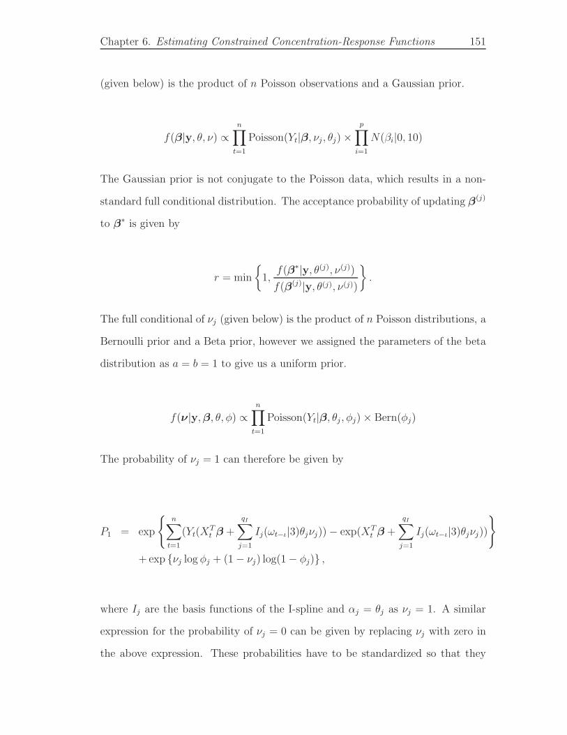
Chapter 6. Estimating Constrained Concentration-Response Functions 151
(given below) is the product of n Poisson observations and a Gaussian prior.
f(β|y, θ, ν) ∝
n∏
t=1
Poisson(Yt|β, νj , θj) ×
p∏
i=1
N(βi|0, 10)
The Gaussian prior is not conjugate to the Poisson data, which results in a non-
standard full conditional distribution. The acceptance probability of updating β(j)
to β∗ is given by
r = min
1,f(β∗|y, θ(j), ν(j))
f(β(j)|y, θ(j), ν(j))
.
The full conditional of νj (given below) is the product of n Poisson distributions, a
Bernoulli prior and a Beta prior, however we assigned the parameters of the beta
distribution as a = b = 1 to give us a uniform prior.
f(ν|y,β, θ, φ) ∝n∏
t=1
Poisson(Yt|β, θj , φj) × Bern(φj)
The probability of νj = 1 can therefore be given by
P1 = exp
n∑
t=1
(Yt(XTt β +
qI∑
j=1
Ij(ωt−ι|3)θjνj)) − exp(XTt β +
qI∑
j=1
Ij(ωt−ι|3)θjνj))
+ exp νj log φj + (1 − νj) log(1 − φj) ,
where Ij are the basis functions of the I-spline and αj = θj as νj = 1. A similar
expression for the probability of νj = 0 can be given by replacing νj with zero in
the above expression. These probabilities have to be standardized so that they

Chapter 6. Estimating Constrained Concentration-Response Functions 152
sum to one.
The most difficult set of parameters to update is θ, and the full conditional dis-
tribution of θj is given by
f(θj |νj ,β,y) ∝n∏
t=1
Poisson(Yt|β, νj, θj) ×
qI∏
j=1
N(θj |0, 10)I[θj>0].
When νj = 1, θj is updated by a Metropolis-Hastings step, using a random walk
proposal distribution. The acceptance probability of updating θ(j) to θ∗ is given
by
rθ = min
f(θ∗|y,β, νj = 1)
f(θ(j)|y,β, νj = 1), 1
The sampling difficulty arises when νj = 0, because the above full conditional dis-
tribution simplifies to a half normal prior, as the data likelihood no longer depends
on θj . Therefore, as this prior is relatively diffuse (variance of 10), excessively large
values could be generated for θj . This in turn would stop νj being estimated as
one in the next iteration of the MCMC algorithm, as the current value of θj would
be too big to be a plausible value under the data likelihood. This would cause
the Markov chain to become stuck. I rectify this problem by updating θj via a
Metropolis-Hastings step, where the proposal distribution only proposes small val-
ues of θj . Note, that values of θj generated in this way do not influence the fitted
CRF, as the corresponding νj values in this situation are always zero.

Chapter 6. Estimating Constrained Concentration-Response Functions 153
As each νj is binary, they are straightforward to update singularly using Gibbs
sampling. The prior probability parameters φj can also be Gibbs sampled, as their
individual full conditionals are beta distributions.
6.4 Simulation Study
In this section I present a simulation study, that assesses the accuracy with which
some of the models described in this paper can estimate concentration-response
functions. Specifically, we compare the estimation performance of the following
four models: (a) a linear model; (b) the B-spline model given by (3.5); (c) the
I-spline model proposed in Section 6.3; and (d) the constrained piecewise linear
model with one change-point proposed by Roberts (2004) (6.1). The first part
of this section describes the study design and data generation, while the second
summarises the results.
6.4.1 Study Design and Data Generation
Two hundred sets of health data are generated under each of 4 different scenarios,
which only differ in the shapes assumed for the concentration-response function
f(·). The functions considered here are displayed in Figure 6.2 and summarised
below, and represent shapes that are likely to be seen in real data.
• Scenario 1 - A linear CRF, f(ωt) = ωtα, where α is chosen so that the
relative risk for a one standard deviation increase in pollution is 1.02, which
is similar to that reported by existing studies.

Chapter 6. Estimating Constrained Concentration-Response Functions 154
0 20 40 60 80
1.00
1.05
1.10
1.15
1.20
1.25
Pollution
True
CR
F
Figure 6.2: The true CRFs for the four scenarios: (1) a linear CRF (solidblack line), (2) a constant CRF (solid gray line), (3) a convex CRF (dashed
line), and (d) a concave CRF (dotted line).
• Scenario 2 - A constant CRF of f(ωt) = 0, which represents the situation
where air pollution has no effect on health.
• Scenario 3 - A non-linear convex relationship, which is similar to the one
estimated for the real data in Section 6.5.
• Scenario 4 - A non-linear concave relationship exhibiting a threshold level,
above which no further effects of air pollution are felt.
Each set of simulated health data is generated from model (3.4) for a period of
1,460 days (4 years), and is based on the covariates and air pollution data used
in the London study presented in Section 6.5. The air pollution data comprise
daily mean ozone concentrations, while the covariates include daily mean temper-
ature and a non-linear time trend. The latter is represented by a natural cubic
Chapter 6. Estimating Constrained Concentration-Response Functions 155
spline with ten degrees of freedom per year, while the former is assumed to have a
non-linear effect on health (modelled by a natural cubic spline with 3 degrees-of-
freedom). The corresponding regression parameters for the temperature covariate
and the non-linear time trend are those estimated from the London analysis in
Section 6.5.
To ensure the results from the two spline based models are not affected by the
number of basis functions selected (i.e. the values of qB and qI), they are imple-
mented with between 1 and 3 interior knots, which corresponds to qB = 2, 3, 4 and
qI = 4, 5, 6. In the next section, the value of (qB, qI) that produces the best set
of results for each model and scenario are presented. Inference for the Bayesian
I-spline model is based on forty thousand MCMC samples, twenty thousand of
which are discarded as burn-in. Finally, the linear change-point model was im-
plemented as suggested in Roberts (2004), where the location of the change-point
was chosen by Akaike’s Information Criterion (AIC).
6.4.2 Results
For each scenario I measure the performance of each model by comparing the true
pollution-health relationship f(·), with the corresponding estimates, fi(·)200i=1,
from the 200 simulated data sets. The true and estimated curves are compared
at ten different pollution concentrations (0, 10, 20, . . . , 80, 90), using the following
two metrics.
1. Median bias - MB(ωj) = Mediani=1,...,200
fi(ωj)
− f(ωj).
2. Median absolute deviation - MAD(ωj) = Mediani=1,...,200
|fi(ωj) − f(ωj)|
.

Chapter 6. Estimating Constrained Concentration-Response Functions 156
Table 6.1: Summary of the simulation study. The table displays the bias,median absolute deviation and the percentage of estimated CRFs that are bio-
logically plausible, for each model and scenario.
Metric ScenarioModel
Linear B-spline I-spline Piecewise1 -0.028 0.049 0.063 -0.728
Bias 2 0.171 0.229 0.032 0.0003 1.613 0.061 0.078 0.0004 -8.651 -2.575 -0.159 -8.6891 1.277 1.925 2.035 1.772
Median absolute 2 1.355 1.858 0.032 0.000Deviation 3 2.888 2.259 0.676 0.839
4 7.451 2.899 3.273 7.4961 99% 68.5% 100% 100%
% Biologically 2 54.5% 14.5% 100% 100%Plausible 3 100% 16% 100% 100%
4 100% 19% 100% 100%
I use median measures of bias and absolute error because the constraints imposed
on the I-spline model cause the distribution of fi(ωj)200i=1 to be skewed. The
results of the study are displayed in Figures 6.3, 6.4 and Table 6.1, the first two
of which display the bias (MB, Figure 6.3) and median absolute deviation (MAD,
Figure 6.4) at each pollution concentration for each model and scenario. In each
case the bias and MAD are presented as a percentage of the value of the true
CRF f(·). The four rows of each figure relate to the four scenarios (row 1 displays
scenario 1 and so on), while each column displays the results from one of the mod-
els. Finally, Table 6.1 summarises the results from each panel of the figures into a
single quantity, namely the median of the bias and MAD across the ten pollution
concentrations.

Chapter 6. Estimating Constrained Concentration-Response Functions 157
The Figures and Table show that when the true CRF is linear (scenario 1) all four
models perform relatively well, with biases generally less than 1% and MAD values
less than 2.5%. The linear model performs the best in this scenario as would be
expected, while the remaining three models produce fairly similar results. When
air pollution has no effect on health (scenario 2) all models again perform rela-
tively well, with biases and MAD values being less than 1% and 2% respectively.
However, in this scenario the I-spline and piecewise linear models outperform the
other two, which is most likely due to the constraints imposed by these models,
that restrict the set of CRFs that can be estimated. In scenarios 3 and 4 the
linear model performs badly as expected, because by design it cannot estimate
non-linear CRFs. In contrast, the I-spline and B-spline models exhibit much bet-
ter performance, as they are designed to capture non-linear shapes. However, in
comparison, the I-spline model generally outperforms the B-spline model, having
biases and MAD values that are either much smaller or only slightly larger. Fi-
nally, the estimates from the B-spline model come at a price, as between 31.5%
and 85.5% of the estimated CRFs are not biologically plausible. This phenomenon
occurs even in the absence of unmeasured confounding, as the covariates used to
generate the health data were included when fitting the model.
6.5 Application - Greater London
I illustrate my methods by presenting a study investigating the effects of ozone
levels on respiratory mortality in Greater London, between 2000 and 2005. It was
possible to use a larger period of data for the analysis in this chapter, compared

Chapter 6. Estimating Constrained Concentration-Response Functions 158
Linear
Pollution
Bia
s
0 40 80
−8
−4
04
B−spline 1 knot
Pollution
Bia
s0 40 80
−8
−4
04
I−spline 3 knots
Pollution
Bia
s
0 40 80
−8
−4
04
Piecewise
Pollution
Bia
s
0 40 80
−8
−4
04
Linear
Pollution
Bia
s
0 40 80
−8
−4
04
B−spline 1 knot
Pollution
Bia
s
0 40 80
−8
−4
04
I−spline 1 knot
Pollution
Bia
s
0 40 80−
8−
40
4
Piecewise
Pollution
Bia
s
0 40 80
−8
−4
04
Linear
Pollution
Bia
s
0 40 80
−8
−4
04
B−spline 2 knots
Pollution
Bia
s
0 40 80
−8
−4
04
I−spline 2 knots
Pollution
Bia
s
0 40 80
−8
−4
04
Piecewise
Pollution
Bia
s
0 40 80
−8
−4
04
Linear
Pollution
Bia
s
0 40 80
−8
−4
04
B−spline 3 knots
Pollution
Bia
s
0 40 80
−8
−4
04
I−spline 1 knot
Pollution
Bia
s
0 40 80
−8
−4
04
Piecewise
Pollution
Bia
s
0 40 80
−8
−4
04
Figure 6.3: Percentage bias for each model and scenario at concentrationsranging between 0 and 90 microns. The four rows depict the results from the
four scenarios.

Chapter 6. Estimating Constrained Concentration-Response Functions 159
02
46
8
Linear
Pollution
MA
D
0 40 800
24
68
B−spline 1 knot
Pollution
MA
D0 40 80
02
46
8
I−spline 3 knots
Pollution
MA
D
0 40 80
02
46
8
Piecewise
Pollution
MA
D
0 40 80
02
46
8
Linear
Pollution
MA
D
0 40 80
02
46
8
B−spline 1 knot
Pollution
MA
D
0 40 800
24
68
I−spline 1 knot
Pollution
MA
D
0 40 80
02
46
8
Piecewise
Pollution
MA
D
0 40 80
02
46
8
Linear
Pollution
MA
D
0 40 80
02
46
8
B−spline 2 knots
Pollution
MA
D
0 40 80
02
46
8
I−spline 2 knots
Pollution
MA
D
0 40 80
02
46
8
Piecewise
Pollution
MA
D
0 40 80
02
46
8
Linear
Pollution
MA
D
0 40 80
02
46
8
B−spline 3 knots
Pollution
MA
D
0 40 80
02
46
8
I−spline 1 knot
Pollution
MA
D
0 40 80
02
46
8
Piecewise
Pollution
MA
D
0 40 80
Figure 6.4: Percentage median absolute deviation for each model and scenarioat concentrations ranging between 0 and 90 microns. The four rows depict the
results from the four scenarios.

Chapter 6. Estimating Constrained Concentration-Response Functions 160
with that of the previous two, as the methods proposed here are not as compu-
tationally intensive and we will not be compared with work in another chapter of
this thesis.
6.5.1 Data
The study region is the city of Greater London, in England, and the data consist
of daily measurements of population health, air pollution and meteorology for the
6 year period between 2000 and 2005. The health data are daily counts of the total
numbers of respiratory mortalities from the population living in the study region,
and exhibit a pronounced yearly cycle, with most deaths occurring in the winter
months, as can be seen from Figure 6.5(a). Daily mean ozone concentrations
were measured at 42 locations across the city, however, 4 of these sites were not
included in this analysis as they did not record ozone concentrations for at least
75% of the duration of the study. The average concentration from the remaining
38 sites was computed to give a representative measure for each day. If any days
still resulted in missing values, after the average was calculated, then these days
were removed from the study to provide a complete case analysis. These data also
exhibit a pronounced yearly cycle, with the highest concentrations occurring in the
summer months (Figure 6.5(b)). Finally, daily mean temperature measured at 16
locations across the city were also obtained, because temperature is known to be
an important confounder in existing air pollution and health studies. In common
with the ozone data, the values at the 16 locations were averaged to produce a
single representative value for each day. As expected these data show a produced
seasonal pattern, which can be seen from Figure 6.5(c).

Chapter 6. Estimating Constrained Concentration-Response Functions 161
2060
100
140
(a)
Date
Num
ber
of d
eath
s
1st Jan 2000 1st Jan 2001 1st Jan 2002 1st Jan 2003 1st Jan 2004 1st Jan 2005 31st Dec 2005
020
6010
0
(b)
Date
O3
1st Jan 2000 1st Jan 2001 1st Jan 2002 1st Jan 2003 1st Jan 2004 1st Jan 2005 31st Dec 2005
05
1525
(c)
Date
Ave
rage
tem
pera
ture
1st Jan 2000 1st Jan 2001 1st Jan 2002 1st Jan 2003 1st Jan 2004 1st Jan 2005 31st Dec 2005
0 5 10 15 20 25 30
2060
100
140
(d)
Average temperature
Num
ber
of d
eath
s
Figure 6.5: Daily counts of (a) respiratory deaths, (b) pollution concentrationsand (c) average temperature in Greater London for the period 2000 to 2005.

Chapter 6. Estimating Constrained Concentration-Response Functions 162
6.5.2 Statistical Modelling
My statistical modelling approach is informed by overall measures of model ad-
equacy, such as AIC, as well as diagnostic plots of the residuals. I first assessed
the confounding effects of temperature, which have previously been highlighted by
Dominici et al. (2002) and Carder et al. (2008). The majority of studies observe a
‘U-shaped’ relationship between temperature and health on the same day, because
increased levels of mortality are observed in very cold and very hot conditions. To
assess if this is the case with my data, I compared models with linear and non-
linear temperature effects, as it was not obvious which should be used from Figure
6.5(d). The non-linear temperature effects were modelled by a natural cubic spline
with a small number of degrees of freedom. A non-linear effect of temperature with
three degrees of freedom is used in this study, because it produced a model with
the lowest AIC. I then assessed the usefulness of including a ‘day of the week’
effect in the model, but as it did not reduce the AIC it was not considered further.
The inclusion of a non-linear temperature effect in the model still leaves a promi-
nent seasonal pattern in the residuals, which I represent by a natural cubic spline
of time (day of the study). A range of degrees of freedom for this seasonal trend
were considered, and the most appropriate value was chosen by comparing plots of
the residuals against time, as well as their autocorrelation and partial autocorre-
lation functions. As a result, ten degrees of freedom per year were chosen, as this
is the smallest value that corresponds to residuals with no trend or short-term
correlation. As the autocorrelation and partial autocorrelation functions of the
residuals from this model exhibit minimal correlation, the assumption of indepen-
dence between the daily health data appears to be valid.

Chapter 6. Estimating Constrained Concentration-Response Functions 163
Finally, daily mean ozone concentrations were added to the model at a lag of one
day, because previous studies (see for example Dominici et al. (2000), Zhu et al.
(2003), and Lee and Shaddick (2008)) have shown that exposure to air pollution is
unlikely to result in health effects on the same day. Four different concentration-
response functions f(·) were applied to the data, which include: (a) a linear model;
(b) the B-spline model given by (3.5); (c) the I-spline model proposed in Section 3;
and (d) the constrained piecewise linear model with one change-point described in
Roberts (2004) (6.1). The optimal levels of smoothness for the two spline models
were chosen by AIC and DIC respectively, which resulted in qB = 4 and qI = 4.
The location of the change-point for the piecewise linear model was also chosen
by AIC, which resulted in a value of 70 µgm−3. Finally, we note, that the AIC
from the 3 non-Bayesian models are; (a) linear = 12,944, (b) B-spline = 12,914,
and (c) piecewise linear = 12,912, which suggests that a linear relationship is not
appropriate for these data.
6.5.3 Results
The estimated concentration-response functions are displayed in Figure 6.6, where
panel (a) displays the estimate from the linear model, panel (b) shows the non-
linear B-spline model, panel (c) presents the estimate from the I-spline model,
while panel (d) relates to the piecewise linear model. In all cases the estimates
(posterior median for the Bayesian I-spline model) are presented as solid lines,
while the dashed lines are 95% uncertainty intervals. All the fitted curves and un-
certainty intervals are presented as relative risks, relative to the minimum ozone
concentration observed during the study period. If f(·) is restricted to be linear,
Chapter 6. Estimating Constrained Concentration-Response Functions 164
increasing ozone concentrations by 20µgm−3 is estimated to result in 2.2% addi-
tional respiratory deaths, with a 95% confidence interval ranging between 0.8%
and 3.5%.
Relaxing this linear restriction without enforcing any shape constraints results in
the concentration-response function shown in panel (b) of Figure 6.6, which ex-
hibits a significantly non-linear shape (a straight line will not fit within the 95%
confidence interval). However, the estimated curve is also unrealistic under the
definition outlined in Section 2.2, because it suggests that ozone is beneficial to
health (as the relative risk is less than one) at concentrations below 60 µgm−3.
Furthermore, the curve decreases at both 0µgm−3 and 35µgm−3, suggesting that
increasing ozone at these concentrations reduces the corresponding health risks.
The concentration-response function estimated from the Bayesian I-spline model
is shown in panel (c), and exhibits a similar overall shape to the estimate from
the B-spline model. However, it does not contain the undesirable features of the
latter estimate described above, and instead exhibits a smooth convex shape. The
fitted curve suggests that no health effects are observed below 20µgm−3, while the
lower part of the 95% credible interval only becomes greater than one at 50µgm−3.
Finally, the constrained piecewise linear model proposed by Roberts (2004) is dis-
played in panel (d), and exhibits the same overall shape as that observed for the
other spline models. However, by design, the curve has a non-smooth change of
trajectory at 70µgm−3, which is unlikely to be realistic.
Finally, I conduct a small sensitivity analysis for the Bayesian I-spline model,
by changing the number of basis functions qI and the prior variance for each
θj . Increasing qI from 4 to 7 has almost no effect on the estimated curve in
Chapter 6. Estimating Constrained Concentration-Response Functions 165
Figure 6.6 panel (c), because the properties P1 to P3 themselves induce a level of
smoothing. The only small effect of increasing qI is that the point at which the
fitted curve becomes greater than zero increases slightly, although the differences
are not large. The impact of changing the variance of the half-normal prior for
θj is also negligible, as varying the value between 1 and 10 has no effect on the
estimated curve.
6.6 Discussion
In this chapter I have proposed a statistical approach for estimating constrained
concentration-response functions between air pollution and health, which are con-
strained to be smooth, non-decreasing, and exhibit no effect in the absence of
pollution. My approach is implemented in a Bayesian setting, and models the
concentration-response function by a monotonic integrated spline. Almost all stud-
ies that estimate (potentially) non-linear CRFs do not enforce any constraints on
their shape, which can result in unrealistic curves being estimated. Such curves
are unlikely to represent the true concentration-response function, and are instead
an artefact of the data set being analysed. My approach thus offers a statisti-
cal solution to this problem, by combining informative prior knowledge about the
likely shape of the concentration-response function, to the information contained
in the data.
The simulation study shows that if the true CRF is linear, then a linear model
is the best model to use. However, it performs very poorly when the true CRF
is non-linear, and as the shape of the latter is not known in advance, using a
non-linear model may be more appropriate. Overall, the I-spline model performs

Chapter 6. Estimating Constrained Concentration-Response Functions 166
Figure 6.6: Relative risk curves and associated 95% confidence (credible)intervals for: (a) a linear relationship; (b) the B-spline model; (c) the Bayesian
I-spline model; and (d) the piecewise linear model.
0 20 40 60 80
0.9
1.0
1.1
1.2
1.3
(a)
Ozone
Rel
ativ
e ris
k
0 20 40 60 80
0.9
1.0
1.1
1.2
1.3
(b)
Ozone
Rel
ativ
e ris
k
0 20 40 60 80
0.9
1.0
1.1
1.2
1.3
(c)
Ozone
Rel
ativ
e ris
k
0 20 40 60 80
0.9
1.0
1.1
1.2
1.3
(d)
Ozone
Rel
ativ
e ris
k

Chapter 6. Estimating Constrained Concentration-Response Functions 167
consistently well across all scenarios, which is not the case for either the B-spline
or piecewise linear models, which exhibit poor results in at least one scenario. In
addition, CRFs estimated from the piecewise linear model have the unattractive
feature of exhibiting sharp change points, which are unlikely to be real effects. Fur-
thermore, the B-spline model regularly produces non-biologically plausible CRFs
even in the absence of unmeasured confounding, a facet not shared by the I-spline
model proposed here.
The concentration-response function estimated for the Greater London data in Sec-
tion 6.5 is convex, exhibiting no health effects for concentrations up to 50 microns,
after which substantial increasing effects are observed. This compares with the
current UK ozone standard of 100 microns (not to be exceeded more than 10 times
a year), suggesting that ozone concentrations below this standard are harmful to
human health. This is also inline with current literature where significant health
risks of ozone have bene found (see for example Verhoeff et al. (1996) and Yang
et al. (2012)). The increasing nature of the curve after 50 microns suggests that if
there is an upper threshold level in ozone concentrations, above which no further
health risks are observed, then it is larger than the concentrations observed in
this study. Bell et al. (2006) found evidence to suggest threshold levels for ozone
presented at very low concentrations suggesting that methods proposed in this
chapter produce results which may not be consistent with the current literature.
The estimated CRF from the B-spline model appears to exhibit random fluctua-
tions around a relative risk of one for ozone concentrations below 50 microns, an
unattractive property which is not shared by the Bayesian I-spline model proposed
here. There may be many possible reasons for this unattractive behaviour, and
it may act as a signal to the researcher that further investigation into the data

Chapter 6. Estimating Constrained Concentration-Response Functions 168
and model may be required. However, if the reason for the random fluctuations
cannot be identified, then one is still left with a non-monotonic curve, which is
highly unlikely to represent the true relationship between air pollution and health.
In the future, I aim to re-analyse data from multi-city studies such as NMMAPS
and APHEA using my approach, which would allow a comparison of my results
with what has previously been found. This would then allow me to estimate
regional and national concentration-response functions over multiple cities, using
meta-analytic methods similar to those employed by Dominici et al. (2002).

Chapter 7
Conclusion
Short-term exposure to air pollution has been associated with cases of both res-
piratory mortality and morbidity. It has been shown to cause and aggravate a
number of respiratory conditions, including asthma, bronchitis and chronic ob-
structive pulmonary disease (COPD). This association between air pollution ex-
posure and risks to human health has been a public health concern for over 700
years. However, it has only become a global topic in the last 80 years primarily due
to the extreme air pollution episodes in the Meuse Valley in 1930 (Firket (1936)),
in Donora, pennsylvania in 1948 (Ciocco and Thompson (1961)) and the London
smog of December 1952 (Ministry of Public Health (1954)), all of which were as-
sociated with a rise in the number of premature deaths. In recent years pollution
levels have dropped considerably, and yet the relationship between air pollution
and human health continues to be an active area of research. The results of such
research has helped shaped environmental legislation, which regulates the major
sources of pollution and sets target levels for ambient air pollution. In the UK
such legislation includes the Clean Air Act (1993) and UK Air Quality Strategy
169

Chapter 7. Conclusion 170
(2007).
The majority of air pollution and health research is based on time series studies,
as opposed to case-crossover or panel studies, as this type of data is routinely
available. Time series studies use aggregate level mortality or morbidity data,
which describes the health of the population living within a geographical region.
An advantage of this type of study is that it is inexpensive and straightforward to
implement and it is also unlikely to be affected by individual level risk factors such
as age and smoking habits. A disadvantage is that only a group level associations
between air pollution exposure and the risks to health can be estimated. This is
thus a much weaker type of analysis, than an individual level study, where cause
and effects can be assessed.
The mortality or morbidity data used in air pollution and health studies are typ-
ically daily counts which often include very small numbers, therefore Poisson re-
gression techniques such as generalised linear or additive models are the most
appropriate. In this thesis I have proposed methods which extend those currently
used in the majority of air pollution and health studies, and I compare their efficacy
against those adopted by the majority of researchers. These developments provide
evidence of deficiencies with the standard modelling approaches. The work which
I have presented in this thesis has been centered around three related themes, with
a particular focus on the air pollution component of the regression model. The
first and second themes related to the measure of ambient air pollution which is
included in the model. The short term health effects of exposure are typically
estimated for a single pollutant. I compare this approach to the health effects of
overall air quality which is the quantity that the population are actually exposed

Chapter 7. Conclusion 171
to. The second theme, which is closely related to the first, is to allow for uncer-
tainty in the pollution estimate and compare the effect this has on the estimated
health effects of overall air pollution. The third and final theme considers the
shape of the estimated concentration-response relationship between air pollution
and the risks to human health. The modelling techniques currently utilised make
no constraints on such a function and as a result can produce unrealistic results.
7.1 Key Theme - Estimating a spatially repre-
sentative measure of overall air quality
Numerous pollutants are measured by the air quality network, including car-
bon monoxide (CO), nitrogen dioxide (NO2), ozone (O3) and particulate matter
(PM10). The majority of epidemiological studies estimate the short-term health
effects of exposure to a single pollutant, for simplicity. However, the air we breathe
and hence are exposed to is a complex mixture of numerous pollutants, including
those previously mentioned. Therefore, the health effects of overall air quality are
of direct public interest. Further to this, the data which are available for air pollu-
tion and health studies includes population level mortality counts which relate to a
study region and point-level measures of these individual pollutants, from within
the study region. This spatial misalignment between point-level pollution data
and the areal-level mortality counts, often termed a change of support problem, is
rectified by creating a representative areal-level measure of pollution. Typically,
this is taken to be the average concentration across the monitoring network. How-
ever, this monitor average is unlikely to be a spatially representative measure of
pollution across the urban area under study, because the locations of the pollution
Chapter 7. Conclusion 172
monitors are unlikely to have been chosen at random or using statistical design
principles. Monitors are typically placed at sites with high pollution concentra-
tions, a phenomenon known as preferential sampling. This is because the monitor
network is primarily used for regulatory purposes. The local environment in which
the monitors are placed, such as next to a main road or in a park, may also be
affected by this phenomenon. Local environment is likely to have a large effect on
the readings from a monitor, this is because one of the main contributors of CO,
NO2 and PM10 concentrations is traffic emissions. The location of the monitors
within a study region is therefore likely to result in the spatially representative
pollution summary being overestimated, which in turn is likely to bias the corre-
sponding health effects. Further to this, the monitors are located at both roadside
and background local environments. Roadside monitors are likely to record par-
ticularly high concentration levels which are unlikely to be a true representative
of what is experienced by the majority of people, who do not spend their time
outside next to main roads.
The calculation of the monitor average does not, therefore, give a true spatial
representation of a pollutants concentrations. Further to this it also does not take
into account the population density across the study region, if the monitors are
therefore located in areas of low population density, then the monitor average may
not directly relate to where a sizeable proportion of the population live. For exam-
ple from Figures 4.1 and 4.4 we saw that the majority of the air pollution monitors
are located in the center of Greater London compared to the majority of the pop-
ulation aged 65 years and above, who live in the suburbs. I therefore, believe that
the appropriate exposure measure is the daily average level of that pollutant to

Chapter 7. Conclusion 173
which the population are exposed. I proposed two different approaches for esti-
mating such a spatially representative measure of a single pollutant. In Chapter 4
I used Bayesian geostatistical methods to model the concentrations of CO, NO2,
O3 and PM10, separately for each day, all of which were recorded by the mon-
itoring network of Greater London for the period 2001 to 2003. This produced
areal-level estimates that were generally lower than the corresponding monitor
averages. One of the reasons for this difference is that the geostatistical model
adjusted for the difference in the pollution concentrations at roadside and back-
ground environments. The posterior predictive distributions for each individual
pollutant were also combined to give a measure of overall air quality. Inference
for the Bayesian geostatistical model is based on direct simulation rather than
Markov chain Monte Carlo methods. This is because the prior distributions of the
parameters are specified specifically to allow for explicit expression of the corre-
sponding posterior distributions. This means that there is no need to remove a
burn-in period as each sample is generated independently. However, a drawback
to the geostatistical model is that it has to be applied to each day of the study
separately for each pollutant. In Chapter 4 this resulted in the application of 4380
(4 pollutants and 1095 days) separate geostatistical analyses. This approach is
therefore computationally expensive. Further to this, a geostatistical model can
only be applied when the pollutant under consideration has been measured at
enough locations to make this type of analysis feasible.
In Chapter 5 I proposed an alternative and simpler approach, which still meets
the aim of producing a spatially representative areal-level estimate of pollution.
This approach models the concentrations for a single pollutant over space and
time simultaneously using a Bayesian regression model. This model incorporated

Chapter 7. Conclusion 174
available covariate information, such as measures of meteorology, to describe the
spatio-temporal pattern in the pollution concentrations. To increase the flexibil-
ity of this model I also proposed the inclusion of a time-varying coefficient, as
this would allow the effects of any covariates which only vary in space to vary
over time. This model was also applied to concentrations of CO, NO2, O3 and
PM10, which were all recorded by the monitoring network in Greater London for
the period 2001 to 2003. With the exception of O3, the areal-level estimates were
generally lower than the corresponding monitor average. This could be because
the proposed model, like the geostatistical model, adjusted for the difference in the
pollution concentrations at roadside and background environments. The slightly
higher results for the areal-level estimate of O3 may be due to the fact that ozone
is not driven by traffic emissions and is instead formed as a chemical reaction in
the atmosphere. To create an index of overall air quality the predictive posterior
distributions for each individual pollutant were combined.
In Chapter 5 I assessed the predictive accuracy of both the geostatistical and the
regression model using the method of cross-validation. The results suggested that
the simpler regression model, proposed in Chapter 5, may over predict the true
concentration levels of a pollutant, despite the fact that this model is able to utilise
all of the available data. Conversely, the geostatistical model, proposed in Chapter
4, under predicts the true concentration levels. However, the geostatistical model
under predicts by less than the regression model over predicts. The results of the
cross-validation also suggest that the simple regression model is very sensitive to
which monitoring sites are included in the model. When three sites which were
located in the centre of London were removed this resulted in the regression model
under predicting the true concentrations. These results suggest that the proposed

Chapter 7. Conclusion 175
regression model is not as good as the geostatistical model proposed in Chapter 4.
7.1.1 Related Theme - Allowing for uncertainty when es-
timating the health risks of air pollution
A further issue with the majority of existing research is that the areal-level pol-
lution estimate, such as the monitor average, is assumed to be a known quantity.
This is despite the true spatially representative measure of pollution being a ran-
dom variable. As a result, the inherent uncertainty in its value should be acknowl-
edged when estimating its health effects. To not account for this uncertainty may
result in the conclusion of significant health risks of pollution when in fact there
is not. Therefore, in addition to producing a spatially representative measure of
overall air quality which can be incorporated into a health model I also took ac-
count of the uncertainty in this estimate of pollution. In both Chapters 4 and 5 I
did this by applying a Bayesian approach to the modelling of a single pollutant.
This meant that for each individual pollutant I achieved a posterior predictive dis-
tribution for each day of the study. I therefore, had a number of estimates which
could be included in a health model. Therefore, I proposed a Bayesian health
model so that the posterior predictive distribution of the spatially representative
pollution measure could be fed through the health model. In both chapters the
main result of interest is the difference in the widths of the uncertainty intervals
between the standard modelling approach and the proposed approach, with the
latter being wider because the uncertainty in the pollution estimate was incorpo-
rated. In both chapters the difference in the width of the uncertainty intervals
resulted in a change in the significance of some of the pollutants. These results

Chapter 7. Conclusion 176
suggest that not accounting for the uncertainty in the estimated value of air pollu-
tion can indeed result in the conclusion of significant health risks when there may
in fact not be any.
7.2 Key Theme - Constraining the relationship
between air pollution and health
For simplicity, the majority of studies estimate a linear Concentration-Response
Function (CRF) between ambient air pollution levels and a health outcome, as it
allows them to summarise the pollution health relationship by a single regression
coefficient. There are a number of studies however, which have tried to relax this
constraint using cubic splines, which restrict the estimated curves to be smooth,
but do not enforce any constraints on their shape. This lack of shape constraints
has resulted in infeasible CRFs being estimated, such as those that exhibit decreas-
ing health effects as the ambient concentrations increase. In Chapter 6 I therefore
proposed a model for estimating constrained concentration response functions be-
tween air pollution and human health.
I constrained the function between air pollution and health to be smooth, non-
decreasing, and exhibit no effect in the absence of pollution, using monotone splines
known as Integrated or I-splines. This provided a set of spline basis functions
which, when combined with non-negative values of the coefficients yields a mono-
tone spline. The use of a spline also provided a fully parametric representation of
the relationship between air pollution and health and made the three constraints
mentioned previously straightforward to implement. I applied a simulation study

Chapter 7. Conclusion 177
to assess the performance of my proposed approach and found that if the true
CRF is linear, then a linear model is indeed the best approach. However, if this is
not the case then a non-linear model is more appropriate. I considered three non-
linear models which were the single change point piecewise linear model proposed
by Roberts (2004), a B-spline model and the I-splines proposed by myself. The
I-spline model performed consistently well across all the proposed scenarios unlike
the B-spline and piecewise linear models. In addition to this the piecewise linear
model had the unattractive feature of exhibiting sharp change points, which are
unlikely to be real effects. The B-spline model also regularly produced infeasible
CRFs.
I applied my proposed model to the data from Greater London for the time period
2000 to 2005. The estimated concentration response function applies to the health
risks associated with ozone concentrations, which were presented on the relative
risk scale. The result of the Bayesian I-spline model was a smooth convex shaped
curve which exhibited none of the undesirable features of the other approaches,
such as sharp change points or suggestions of air pollution being beneficial to hu-
man health. As this method uses spline basis functions, the number of knots for
which must be chosen by either the user or some selection algorithm, I also con-
ducted a small sensitivity analysis. I found that increasing the number of knots
from 4 to 7 had almost no effect on the resulting CRF except to change slightly
the point at which the fitted curve becomes greater than zero.

Chapter 7. Conclusion 178
7.2.1 Limitations
In this thesis I have attempted to extend the current methodology used to estimate
the association between air pollution exposure and the risks to human health. I
have compared the efficacy of my proposed approaches with those adopted by the
majority of researchers and found evidence of deficiencies with the standard ap-
proach. However, the methods that I have proposed are only a possible solution
to some of the problems which exist in the current literature. Many new methods
are being explored and developed every day, many of which will undoubtedly su-
persede or find flaws with the those which I have proposed.
The methods proposed in both Chapters 4 and 5 combine a spatially representa-
tive measure of a number of single pollutants to create a single measure of overall
air quality. One of the limitations of this approach is that this measure of overall
air quality is made up of only four pollutants when in fact a great deal more exist
and are measured by monitoring networks. Further to this each pollutant was
treated as if it is independent from the other three. However, this is perhaps not
the case as some of the pollutants may be in each others causal path way. Perhaps
more thought should also be given to which pollutants should be included in such
measures. It is perhaps not necessary to include as many pollutants as possible,
particularly if some of those pollutants are by products of each other. In addition,
the simple average aggregation method I used to create the air quality index is
only one possible method. There are many other possible approaches to this and it
may have been more prudent to have attached weights to the individual pollutants
based on their perceived levels of danger to human health. Alternatively, these
weights could be random and determined by the data, as an additional level in the

Chapter 7. Conclusion 179
Bayesian health model. A further piece of work could be to combine the positive
aspects of both the geostatistical model proposed in Chapter 4 and the regression
model proposed in Chapter 5 to create a non-separable spatio-temporal model.
Another possibility is to consider the use of multivariate geostatistics which would
allow the user to pool the data from multiple pollutants (for example see Amir
et al. (2011) and Degan et al. (2006)), thus allowing for a borrowing of strength
across pollutants when making the spatial predictions.
As the models proposed in Chapters 4 and 5 are both presented as possible solu-
tions to the problem of estimating a spatially representative measure of overall air
quality I attempted to compare the predictive accuracy of each approach via the
method of cross validation. This was not meant as a conclusive assessment of the
predictive accuracy of each model but more as an informal means of comparing
each model. However, the use of the method of cross-validation was perhaps a
poor choice as the issue of this technique in the presence of highly correlated data
has been well documented. Further to this, had this method been suitable the ar-
bitrary choice of constructing only five scenario cases may not have been suitable.
Had more scenario cases of test and validation data been created it could have
been found that the results of scenario 3 were what should have been expected
and those of the remaining scenarios were exceptional cases.
In Chapter 6 I only estimated the health effects of a single pollutant. While
this pollutant is frequently investigated by other studies, due to its known health
risks, it is still only a single pollutant and does not represent the air we breathe.
Further to this, I only included the monitor average, which is known to not be a

Chapter 7. Conclusion 180
truly representative measure of the amount of ozone the population are exposed to.
In this thesis I used data relating to the area of Greater London which I found, like
many real life data sets, to be overdispersed. However, regardless of this I chose
to ignore this aspect of the data and instead model the respiratory mortality as if
they had arisen from a Poisson distribution, which assumes a specific mean vari-
ance relationship (equal mean and variance). While the model parameters may
have been unaffected by this, any associated uncertainty interval may be afflicted
by bias. This could mean that the conclusions drawn about the methods proposed
in each of Chapters 4, 5 and 6 could be incorrect. In the future I would like to
compare the results of the proposed methods in Chapters 4 to 6 with those which
would have been found had I accounted for overdispersion via one of the suitable
methods which were discussed in Section 3.4. A further limitation of the work
presented in this thesis is the use of a single lag which was arbitrarily chosen.
This overly simplistic method was used to facilitate the comparison of the results
presented in Chapters 4 and 5. However, a moving-average over a number of days
may have been more suitable, as each pollutant is likely to have significant health
effects at a number of different lags. Had I used a moving-average over a large
enough time period I should still have been able to compare my results for each
pollutant and overall air quality. Alternatively, a distributed lag model could have
been used, again over a large enough time period to facilitate the comparison of
the results. This would have meant including the lags for several consecutive days
in the model and constraining the shape of the associated coefficients.
In the future I would like to perform a simulation study in order to better compare
the two models proposed in Chapters 4 and 5. Ultimately however, I would like to

Bibliography 181
combine the motivations which were presented in all three chapters, and therefore
include a spatially representative measure of overall air quality in a model which
is constrained to give realistically shaped concentration-response functions.

Bibliography
Akaike, H. (1974). A new look at the statistical model identification. IEEE
Transactions on Automatic Control 19, 716 – 723.
Alessandrini, E., S. Zauli Sajani, F. Scotto, R. Miglio, S. Marchesi, and P. Lauriola
(2011). Emergency ambulance dispatches and apparent temperature: A time
series analysis in Emilia-Romagna, Italy. Environmental Research 111, 1192 –
1200.
Almon, S. (1965). The distributed lag between capital appropriations and expen-
ditures. Econometrica 33, 178 – 196.
Amir, K., M. Meshkani, and M. Mohsen (2011). Spatial analysis of auto-
multivariate lattice data. Statistical Papers 52, 937 – 952.
Andersen, Z., P. Wahlin, O. Raaschou-Nielsen, M. Ketzel, T. Scheike, and S. Loft
(2008). Size distribuiton and total number concentration of ultrafine and ac-
cumulation mode particles and hospital admissions in children and the elderly
in Copenhagen, Denmark. Occupational and Environmental Medicine 65, 458 –
466.
Baccini, M., A. Biggeri, P. Grillo, D. Consonni, and P. Bertazzi (2011). Health
impact assessment of fine particle pollution at the regional level. American
Journal of Epidemiology 174, 1396 – 1405.
182

Bibliography 183
Ballester, F., M. Saez, S. Perez-Hoyos, C. Inıguez, A. Gandarillas, A. Tobıas,
J. Bellido, M. Taracido, F. Arribas, A. Daponte, E. Alonso, A. Canada,
F. Guillen-Grima, L. Cirera, M. Perez-Boıllos, C. Saurina, F. Gomez, and
J. Tenıas (2002). The EMECAM project: a multicentre study on air pollu-
tion and mortality in Spain: Combined results for particulates and for sulphur
dioxide. Occupational and Environmental Medicine 59, 300 – 308.
Barca, E., G. Passarella, and V. Uricchio (2008). Optimal extension of the rain
gauge monitoring network of the Apulian Regional Consortium for crop protec-
tion. Environmental Montioring and Assessment 145, 375 – 386.
Bell, M. and D. Davies (2001). Reassessment of the lethal London fog of 1952:
novel indicators of acute and chronic consequneces of acute exposure to air
pollution. Environmental Health Perspectives 109, 389 – 394.
Bell, M., R. Peng, and F. Dominici (2006). The exposure-response curve for ozone
and risk of mortality and the adequacy of current ozone regulations. Environ-
mental Health Perspectives 114, 532 – 536.
Breslow, N. (1990). Tests of hypotheses in overdispersed Poisson regression and
other quasi-likelihood models. Journal of the American Statistical Associa-
tion 85, 565 – 571.
Bruno, F. and D. Cocchi (2002). A unified strategy for building simple air quality
indices. Environmetrics 13, 243 – 261.
Buhlmann, P. and B. Yu (2003). Boosting with the L-2 loss: Regression and
classification. Journal of the American Statistical Association 98, 324 – 339.

Bibliography 184
Carder, M., R. McNamee, I. Beverland, R. Elton, G. Cohen, J. Boyd, and R. Agius
(2005). The lagged effect of cold temperature and wind chill on cardiorespiratory
mortality in Scotland. Occupational and Environmental Medicine 62, 702 – 710.
Carder, M., R. McNamee, I. Beverland, R. Elton, M. Van Tongeren, G. Cohen,
J. Boyd, W. MacNee, and R. Agius (2008). Interacting effects of particulate
pollution and cold temperature on cardiorespiratory mortality in Scotland. Oc-
cupational and Environmental Medicine 65, 197 – 204.
Cerutti, B., C. Tereanu, G. Domenighetti, E. Cantoni, M. Gaia, I. Bolgiani,
M. Lazzaro, and I. Cassis (2006). Temperature related mortality and ambulance
service interventions during the heat waves of 2003 in Ticino (Switzerland). So-
cial and Preventitive Medicine 51, 185 – 193.
Charnes, A., E. Frome, and P. Yu (1976). The equivalence of generalized least
squares and maximum likelihood estimates in the exponential family. Journal
of the American Statistical Association 71, 169 – 171.
Chen, R., G. Pan, H. Kan, J. Tan, W. Song, Z. Wu, X. Xu, Q. Xu, C. Jiang, and
B. Chen (2010). Ambient air pollution and daily mortality in Anshan, China:
A time-stratified case-crossover analysis. Science of the Total Environment 408,
6086 – 6091.
Chiogna, M. and C. Gaetan (2002). Dynamic generalized linear models with ap-
plication to environmental epidemiology. Journal of the Royal Statistical Society
Series C 51, 453 – 468.
Ciocco, A. and D. Thompson (1961). A follow-up of Donora ten years after:
Methodology and findings. American Journal of Public Health 51, 155 – 164.

Bibliography 185
Cocchi, D., F. Greco, and C. Trivisano (2007). Hierarchical space-time modelling
of PM10 pollution. Atmospheric Environment 41, 532 – 542.
Collings, B. and B. Margolin (1985). Testing goodness of fit for the Poisson
assumption when observations are not identically distributed. Journal of the
American Statistical Association 80, 411 – 418.
Cox, D. (1983). Some remarks on overdispersion. Biometrika 70, 269 – 274.
Cressie, N. (1993). Statistics for spatial data (1st ed.). Wiley Series in Probabaility
and Statisitcs.
Curriero, F., K. Heiner, J. Samet, S. Zeger, L. Strug, and J. Patz (2002). Temper-
ature and mortality in 11 cities of the Eastern United States. American Journal
of Epidemiology 155, 80 – 87.
Daniels, M., F. Dominici, J. Samet, and S. Zeger (2000). Estimating particulate
matter-mortality dose-response curves and threshold levels: An anlysis of daily
time-series for the 20 largest US cities. American Journal of Epidemiology 152,
397 – 406.
Daniels, M., F. Dominici, S. Zeger, and J. Samet (2004). The National Morbid-
ity, Mortality, and Air Pollution Study Part III: PM10 Concentration-response
curves and thresholds for the 20 largest US cities. Research Report Health Effects
Institute Project , 1 – 21.
Dean, C. and J. Lawless (1989). Tests for detecting overdispersion in Poisson
regression models. Journal of the American Statistical Association 84, 467 –
472.

Bibliography 186
Degan, G., G. Di Bona, D. Lippiello, and M. Pinzari (2006). PM10 dispersion
model in quarrying activites: A comparison of an ISC3 approach to a mono/-
multivariate geostatistical estimation. Transaction of the Wessex Institute 86,
111 – 120.
Department for Environemnt, Food and Rural Affairs (2007). The Air Quality
strategy for England, Scotland, Wales and Northern Ireland. Vol. 1. Stationary
Office.
Diaz, J., A. Tobias, and C. Linares (2012). Saharn dust and association be-
tween particulate matter and case-specific mortality: A case-crossover analysis
in Madrid (Spain). Environmental Health 11, 1 – 6.
Diggle, P., R. Menezes, and T. Su (2010). Geostatistical inference under preferen-
tial sampling (with discussion). Journal of the Royal Statistical Society, Series
C 59, 191 – 232.
Diggle, P. and P. Ribeiro Jr (2007). Model-based geostatistics (1st ed.). Springer
Series in Statistics.
Dobson, A. and A. Barnett (2008). An Introduction to Generalized Linear Models
(3rd ed.). Chapman and Hall/CRC Press, London.
Dockery, D., C. Pope, X. Xu, J. Spengler, J. Ware, M. Fay, B. Ferris, and F. Speizer
(1993). An association between air pollution and mortlaity in six US cities. The
New England Journal of Medicine 329, 1753 – 1759.
Dominici, F., M. Daniels, S. Zeger, and J. Samet (2002). Air pollution and mor-
tality: Estimating regional and national dose-response relationships. Journal of
the American Statistical Association 97, 100 – 111.

Bibliography 187
Dominici, F., A. McDermott, S. Zeger, and J. Samet (2002). On the use of general-
ized additive models in time-series studies of air pollution and health. American
Journal of Epidemiology 156, 193 – 203.
Dominici, F., A. McDermott, S. Zeger, and J. Samet (2003). Airborne particulate
matter and mortality: Timescale effects in four US cities. American Journal of
Epidemiology 157, 1055 – 1065.
Dominici, F., R. Peng, M. Bell, L. Pham, A. McDermott, S. Zeger, and J. Samet
(2006). Fine particulate air pollution and hospital admission for cardiovascular
and respiratory diseases. American Medical Association 295, 1127 – 1134.
Dominici, F., J. Samet, and S. Zeger (2000). Combining evidence on air pollution
and daily mortality from the 20 largest US cities: A hierarchical modelling
strategy. Journal of the Royal Statistical Society, Series A 163, 263 – 302.
Dominici, F., L. Sheppard, and M. Clyde (2003). Health effects or air pollution:
A statistical review. International Statistical Review 71, 243 – 276.
Efron, B. (1986). Double exponential families and their use in generalized linear
regression. Journal of the American Statistical Association 81, 709 – 721.
Eilers, P. and B. Marx (1996). Flexible Smoothing with B-splines and penalties.
Statistical Science 11, 89 – 121.
Firket, J. (1936). Fog along the Meuse Valley. Transactions of the Faraday Soci-
ety 32, 1192 – 1197.
Gelfand, A., L. Zhu, and B. Carlin (2001). On the change of support problem for
spatio-temporal data. Biostatistics 2, 31 – 45.
Bibliography 188
Gelman, A. (2006). Prior distributions for variance parameters in hierarchical
models. Bayesian Analysis 1, 515 – 533.
Gelman, A., J. Carlin, H. Stern, and D. Rubin (2004). Bayesian Data Analysis
(2nd ed.). Chapman and Hall/CRC Press, London.
Gelman, A. and J. Hill (2007). Data analysis using regression and multilevel/hier-
archical model (1st ed.). Cambridge University Press.
Gelman, A. and D. Rubin (1992). Inference from iterative simulation using mut-
liple sequences (with discussion). Statistical Science 7, 457 – 511.
Gold, D., A. Litonjua, J. Schwartz, E. Lovett, A. Larson, B. Nearing, G. Allen,
M. Verrier, R. Cherry, and R. Verrier (2000). Ambient pollution and heart rate
variability. Circulation 101, 1267 – 1273.
Goldberg, M., R. Burnett, J. Bailar, J. Brook, Y. Bonvalot, R. Tamblyn, R. Singh,
and M. Valois (2001). The association between daily mortality and ambient air
particle pollution in Montreal, Quebec. Environmental Research Section A 86,
12 – 25.
Hastie, T. and R. Tibshirani (1990). Generalized Additive Models (1st ed.). Chap-
man and Hall/CRC Press, London.
Hastie, T. and R. Tibshirani (1993). Varying-coefficient models. Journal of the
Royal Statistical Society, Series B 55, 757 – 796.
Health Effects Institute (2003). Assessing health impact of air quality regulations:
Concepts and methods for accountability research. Boston, MA: HEI Account-
ability Working Group. HEI Communication 11 .

Bibliography 189
Hong, Y., J. Leem, E. Ha, and D. Christiani (1999). PM10 exposure, gaseous
pollutants, and daily mortality in Inchon, South Korea. Environmental Health
Perspectives 107, 873 – 878.
Huang, Y., F. Dominici, and M. Bell (2005). Bayesian hierarchical distributed lag
models for summer ozone exposure and cardio-respiratory mortality. Environ-
metrics 16, 547 – 562.
Huynen, M., P. Martens, D. Schram, M. Weijenberg, and A. Kunst (2001). The
impact of heat waves and cold spells on mortality rates in the Dutch population.
Environmental Health Perspectives 109, 463 – 470.
Jerrett, M., R. Burnett, R. Ma, C. Pope III, D. Krewski, K. Newbold, G. Thurston,
Y. Shi, N. Finkelstein, E. Calle, and M. Thun (2005). Spatial analysis of air
pollution and mortality in Los Angeles. Epidemiology 16, 727 – 736.
Kan, H., S. London, H. Chen, G. Song, G. Chen, L. Jiang, N. Zhao, Y. Zhang, and
B. Chen (2007). Diurnal temperature range and daily mortaltiy in Shanghai,
China. Environmental research 103, 424 – 431.
Katsouyanni, K., J. Schwartz, C. Spix, G. Touloumi, D. Zmirou, A. Zanobetti,
B. Wojtyniak, J. Vonk, A. Tobias, A. Ponka, S. Medina, L. Bacharova, and
H. Anderson (1996). Short term effects of air pollution on health: A European
approach using epidemiologic time series data: The APHEA protocol. Journal
of Epidemiology and Community Health 50, S12 – S18.
Kelsall, J., S. Zeger, and J. Samet (1999). Frequency domain log-linear models; Air
pollution and mortality. Journal of the Royal Statistical Society, Series C 48,
331 – 344.

Bibliography 190
Klebanoff, M. and S. Cole (2008). Use of multiple imputation in the epidemiologic
literature. American Journal or Epidemiology 168, 355 – 357.
Knorr-Held, L. (1999). Conditional prior proposals in dynamic models. Scandina-
vian Journal of Statistics 26, 129 – 144.
Kysely, J., L. Pokorna, J. Kyncl, and B. Kriz (2009). Excess cardiovascular mor-
tality associated with cold spells in the Czech Republic. BMC Public Health 9,
Article No. 19.
Kyung, P., H. Chul, and K. Ho (2011). Effect of changes on mortality associated
with air pollution in Seoul, Korea. Journal of Epidemiology and Community
Health 65, 368 – 375.
Laden, F., L. Neas, D. Dockery, and J. Schwartz (2000). Association of fine
particulate matter from different sources with daily mortality in six US cities.
Environmental Health Perspectives 108, 941 – 947.
Lambert, D. and K. Roeder (1995). Overdispersion diagnostics for generalized
linear models. Journal of the American Statistical Association 90, 1225 – 1236.
Lee, D., C. Ferguson, and E. Marian Scott (2011). Constructing representative air
quality indicators with measures of uncertainty. Journal of the Royal Statistical
Society, Series A 174, 109 – 126.
Lee, D. and G. Shaddick (2007). Time-varying coefficient models for the analysis
of air pollution and health outcome data. Biometrics 63, 1253 – 1261.
Lee, D. and G. Shaddick (2008). Modelling the effects of air pollution on health
using Bayesian dynamic generalised linear models. Environmetrics 19, 785–804.

Bibliography 191
Lee, D. and G. Shaddick (2010). Spatial modeling of air pollution in studies of its
short term health effects. Biometrics 66, 1238 – 1246.
Leitenstorfer, J. and G. Tutz (2007). Generalized monotonic regression based on
B-splines with an application to air pollution data. Biostatistics 8, 654 – 673.
Lin, M., Y. Chen, R. Burnett, P. Villeneuve, and D. Krewski (2002). The influence
of ambient coarse particulate matter on asthma hospitalization in children: Case
crossover and time-series analysis. Environemntal Health Perspectives 110, 575
– 581.
Lipfert, F. (1993). A critical review of studies of the association between demands
for hospital services and air pollution. Environemntal Health Perspective 101,
229 – 268.
Loperfido, N. and P. Guttorp (2008). Network bias in air quality monitoring
design. Environmetrics 19, 661 – 671.
Ma, Y., R. Chen, G. Pan, X. Xu, W. Song, B. Chen, and H. Kan (2011). Fine
particulate air pollution and daily mortality in Shenyang, China. Science of
Total Environment 409, 2473 – 2477.
Mallone, S., M. Stafoggia, A. Faustini, G. Gobbi, A. Marconi, and F. Forastiere
(2011). Saharan dust and associations between particulate matter and daily
mortality in Rome, Italy. Environmnetal Health Perspectives 119, 1409 – 1414.
Mar, T., G. Norris, J. Koenig, and T. Larson (2000). Associations between air
pollution and mortality in Phoenix, 1995 - 1997. Environmental Health Perspec-
tives 108, 347 – 353.

Bibliography 192
Matern, B. (1960). Spatial variation. stochastoc models and their application to
some problems in forest surveys and other sampling investigations. Meddelanden
fran Statens Skogsforskningsinstitut 49, 144.
Matheron, G. (1963). Principles of geostatistics. Economic Geology 58, 1246 –
1266.
McCullagh, P. and J. Nelder (1989). Generalised Linear Models (2nd ed.). Chap-
man and Hall/CRC Press, London.
Ministry of Public Health (1954). Mortality and morbidity during the London
smog of December 1952. H.M. Stationary Office.
Moolgavkar, S., E. Luebeck, T. Hall, and E. Anderson (1995). Air pollution and
daily mortality in Philadelphia. Epidemiology 6, 476 – 484.
Murray, C. and C. Nelson (2000). State-space modeling of the relationship be-
tween air quality and mortality. Journal of the Air and Waste Management
Association 50, 1075 – 1080.
Neas, L., J. Schwartz, and D. Dockery (1999). A case-crossover analysis of air
pollution and mortality in Philadelphia. Environmental Health Perspectives 107,
629 – 631.
Nelder, J. and R. Wedderburn (1972). Generalized linear models. Journal of the
Royal Statistical Society, Series A 135, 370 – 384.
O’Hara, R. and M. Sillanpaa (2009). A review of bayesian variable selection
methods: What, how and which. Bayesian Analysis 4, 85 – 118.
Ott, W. (1978). Environmental indices: Theory and Practice. Ann Arbor Science
Publishers: Ann Arbor.
Bibliography 193
Paramo, J. and U. Saint-Paul (2012). Spatial structure of the Caribbean lobster
(Metanephrops binghami) in the Colombian Caribbean Sea. Helgoland Marine
Research 66, 25 – 31.
Parikh, J. (2011). Hardships and health impacts on women due to traditional
cooking fuels: A case study of Himachal Pradesh, India. Energy Policy 39, 7587
– 7594.
Patinha, C., A. Reis, C. Dias, A. Cachada, R. Adao, H. Martins, E. Ferreira da
Silva, and A. Sousa (2012). Lead availability in soils from Portugal’s Centre
Region with special reference to bioaccessibility. Environmental Geochemistry
and Health 34, 213 – 227.
Peng, R. and M. Bell (2010). Spatial misalignment in time series studies of air
pollution and health data. Biostatistics 11, 720 – 740.
Peng, R., F. Dominici, and T. Louis (2006). Model choice in time series studies
of air pollution and mortality. Journal of the Royal Statistical Society, Series
A 169, 179 – 203.
Peng, R., F. Dominici, R. Pastor-Barriuso, S. Zeger, and J. Samet (2005). Seasonal
analyses of air pollution and mortality in 100 US cities. American Journal of
Epidemiology 161, 585 – 594.
Peters, A., E. Liu, R. Verrier, J. Schwartz, D. Gold, M. Mittleman, J. Baliff, A. Oh,
G. Allen, K. Monahan, and D. Dockery (2000). Air pollution and incidence of
cardiac arrhythmia. Epidemiology 11, 11 – 17.
Peters, A., J. Skorkovsky, F. Kotesovec, J. Brynda, C. Spix, H. Wichmann, and
J. Heinrich (2000). Associations between mortality and air pollution in Central
Europe. Environmental Health Perspectives 108, 283 – 287.

Bibliography 194
Pitard, A. and J. Viel (1997). Some methods to address collinearity among pollu-
tants in epidemiological time series. Statistics in Medicine 16, 527 – 544.
Pope III, C., R. Burnett, M. Thun, E. Callee, D. Krewski, K. Ito, and G. Thurston
(2002). Lung cancer, cardiopulmonary mortality, and long-term exposure to fine
particulate air pollution. Journal of the American Medical Association 287, 1132
– 1141.
Pope III, C. and D. Dockery (2006). Health effects of fine particulate air pollution:
Lines that connect. Journal of the Air and Waste Management Association 56,
709 – 742.
Pope III, C. and J. Schwartz (1996). Time series for the analysis of pulmonary
health data. American Journal of Respiratory and Critical Care Medicine 154,
S229 – S233.
Pope III, C., M. Thun, M. Namboodiri, D. Dockery, J. Evans, F. Speizer, and
C. Heath (1995). Particulate air pollution as a predictor of mortality in a
prospective study of U.S. adults. American Journal of Respiratory and Critical
care Medicine 151, 669 – 674.
Pringle, M., B. Marchant, and R. Lark (2008). Analysis of two variants of a
spatially distributed crop model, using wavelet transforms and geostatistics.
Agricultural Systems 98, 135 – 146.
R Development Core Team (2011). R: A Language and Environment for Statistical
Computing. Vienna, Austria: R Foundation for Statistical Computing. ISBN
3-900051-07-0.
Ramsay, J. (1988). Monotone regression splines in action. Statistical Science 3,
425 – 461.
Bibliography 195
Ribeiro Jr., P. and P. Diggle (2001). geoR: a package for geostatistical analysis.
R-NEWS 1 (2), 15–18.
Roberts, S. (2004). Biologically plausible particulate air pollution mortality con-
centration response functions. Environmental Health Perspectives 112, 309 –
313.
Roberts, S. and P. Switzer (2004). Mortality displacement and distributed lag
models. Inhalation Toxicology 16, 879 – 888.
Rubin, D. (1984). Bayesianly justifiable and relevant frequency calculations for
the applied statistician. The Annals of Statistics 12, 1151 – 1172.
Ruggieri, M. and A. Plaia (2012). An aggregate AQI: Comparing different stan-
dardizations and introducing a variability index. Science of the Total Environ-
ment 420, 263 – 272.
Ruppert, D., M. Wand, and R. Carroll (2005). Semiparametric Regression (2nd
ed.). Cambridge University Press.
Samet, J., S. Zeger, F. Dominici, F. Curriero, I. Coursac, D. Dockery, J. Schwartz,
and A. Zanobetti (2000). The National Morbidity, Mortality, and Air Pollution
study. Part II: Morbidity and mortality from air pollution in the United States.
Health Effects Institute Project Report 94 96-97, 5 – 47.
Samoli, E., A. Analitis, G. Touloumi, J. Schwartz, H. Anderson, J. Sun-
yer, L. Bisanti, D. Zmirou, J. Vonk, J. Pekkanen, P. Goodman, A. Paldy,
C. Schindler, and K. Katsouyanni (2005). Estimating the exposure response
relationships between particulate matter and mortality within the APHEA mul-
ticity project. Environmental Health Perspectives 113, 88 – 95.

Bibliography 196
Samoli, E., A. Zanbetti, J. Schwartz, R. Atkinson, A. LeTertre, C. Schindler,
L. Perez, E. Cadum, J. Pekkanen, A. Paldy, G. Touloumi, and K. Katsouyanni
(2009). The temporal pattern of mortality reponses to ambient ozone in the
APHEA project. Journal of Epidmiology and Community Health 63, 960 – 966.
Sarnat, S., A. Raysoni, W. Li, F. Holguin, B. Johnson, S. Flores Luevano, J. Gar-
cia, and J. Sarnat (2012). Air pollution and acute respiratory response in a
panel of asthmatic children along the U.S. - Mexico border. Environmental
Health perspectives 120, 437 – 444.
Schwartz, J. (1991). Particulate air pollution and daily mortality in Detroit. En-
vironemntal Research 56, 204 – 213.
Schwartz, J. (1993). Air pollution and daily mortality in Birmingham, Alabama.
American Journal of Epidemiology 137, 1136 – 1147.
Schwartz, J. (1994). Nonparametric smoothing in the analysis of air pollution and
respiratory illness. The Canadian Journal of Statistics 22, 471 – 487.
Schwartz, J. (2000). Harvesting and long-term exposure effects in the relationship
between air pollution and mortality. American Journal of Epidemiology 151,
440 – 448.
Schwartz, J. (2001). Is there harvesting in the association of airborne particles
with daily deaths and hospital admissions? Epidemiology 12, 55 – 61.
Schwartz, J., F. Ballester, M. Saez, S. Perez-Hoyos, J. Bellido, K. Cambra, F. Ar-
ribas, A. Ca(n)ada, M. Perez-Boillos, and J. Sunyer (2001). The concentration-
response relation between air pollution and daily deaths. Environmental Health
Perspectives 109, 1001 – 1006.

Bibliography 197
Schwartz, J. and A. Marcus (1990). Mortality and air pollution in London: A
time series analysis. American Journal of Epidemiology 131, 185 – 194.
Schwarz, G. (1978). Estimating the dimension of a model. The Annals of Statis-
tics 6, 461 – 464.
Semenza, J., J. McCullough, W. Flanders, M. McGeehin, and J. Lumpkin (1999).
Excess hospital admissions during the July 1995 heat wave Chicago. American
Journal of Preventive Medicine 16, 269 – 277.
Shaddick, G., D. Lee, J. Zidek, and R. Salway (2008). Estimating exposure re-
sponse functions using ambient pollution concentrations. The Annals of Applied
Statistics 2, 1249 – 1270.
Shaddick, G. and J. Wakefield (2002). Modelling daily multivariate pollutant data
at multiple sites. Journal of the Royal Statistical Society, Series C 51, 351 –
372.
Sheffield, P., K. Knowlton, J. Carr, and P. Kinney (2011). Modeling of regional
climate change effects on ground-level ozone and childhood asthma. American
Journal of Preventative Medicine 41, 251 – 257.
Sherman, M. (2011). Spatial Statistics and Spatio-Temporal Data: Covariance
Functions and Directional Properties (1st ed.). John Wiley and Sons.
Shooter, D. and P. Brimblecombe (2009). Air quality indexing. International
Journal of Environment and Pollution 36, 305 – 323.
Smith, R., J. Davis, J. Sacks, P. Speckman, and P. Styer (2000). Regression
models for air pollution and daily mortality: analysis of data from Birmingham,
Alabama. Environmetrics 11, 719 – 743.

Bibliography 198
Spiegelhalter, D., N. Best, B. Carlin, and A. Van der Linde (2002). Bayesian
measures of model complexity and fit. Journal of the Royal Statistical Society,
Series B 64, 583–639.
Spix, C., J. Heinrich, D. Dockery, J. Schwartz, G. Volksch, K. Schwinkowski,
C. Collen, and H. Wichmann (1993). Air pollution and daily mortality in Erfurt,
East Germany, 1980-1989. Environmental Health Perspectives 101, 518 – 526.
Tao, Y., L. Zhong, X. Huang, S. Lu, Y. Li, L. Dai, Y. Zhang, T. Zhu, and W. Huang
(2011). Acute mortality effects of carbon monoxide in the Pearl River Delta of
China. Science of the Total Environment 410, 34–40.
Terzano, C., F. Di Stefano, V. Conti, E. Graziani, and A. Petroianni (2010). Air
pollution ultrafine particles: toxicity beyond the lung. European Review for
Medical and Pharmacological Sciences 14, 809–821.
Touloumi, G., R. Atkinson, A. Le Tertre, E. Samoli, J. Schwartz, C. Schindler,
J. Vonk, G. Rossi, M. Saez, D. Rabszenko, and K. Katsouyanni (2004). Analysis
of health outcome time series data in epidemiological studies. Environmetrics 15,
101 – 117.
Van den Elshout, S. and K. Leger (2006). Comparing urban air quality across
borders. Technical report.
Vedal, S., M. Brauer, R. White, and J. Petkau (2003). Air pollution and daily
mortality in a city with low levels of pollution. Environmental Health Perspec-
tives 111, 45 – 52.
Verhoeff, A., G. Hoek, J. Schwartz, and J. van Wijen (1996). Air pollution and
daily mortality in Amsterdam. Epidemiology 7, 225 – 230.

Bibliography 199
Violato, M., S. Petrou, and R. Gray (2009). The relationship between household
income and childhood respiratory health in the United Kingdom. Social Science
and Medicine 69, 955 – 963.
Wakefield, J. and R. Salway (2001). A statistical framework for ecological and
aggregate studies. Journal of the Royal Statistical Society, Series A 164, 119 –
137.
Wand, M. (2000). A comparison of regression spline smoothing procedures. Com-
putational Statistics 15, 443 – 462.
Wedderburn, R. (1974). Quasi-likelihood functions, generalized linear models, and
the Gauss-Newton method. Biometrika 61, 439 – 447.
Wilmhurst, P. (1994). Temperature and cardiovascular mortality. British Medical
Journal 309, 1029 – 1030.
Yang, C., H. Yang, S. Guo, Z. Wang, X. Xu, X. Duan, and H. Kan (2012). Al-
ternative ozone metrics and daily mortality in Suzhou: The China air pollution
and health effects study (CAPES). Science of the Total Environment 426, 83 –
89.
Ye, X., R. Wolff, W. Yu, P. Vaneckova, X. Pan, and S. Tong (2012). Ambient tem-
perature and morbidity: A review of epidemiological evidence. Environmental
Health Perspectives 120, 19 – 28.
Yu, O., L. Sheppard, T. Lumley, J. Koenig, and G. Shapiro (2000). Effects of
ambient air pollution on symptoms of asthma in Seattle-area children enrolled
in the CAMP study. Environmental Health Perspectives 108, 1209 – 1214.
Zanobetti, A., J. Schwartz, E. Samoli, A. Gryparis, G. Touloumi, R. Atkin-
son, A. Le Terte, J. Bobros, M. Celko, A. Goren, B. Forsberg, P. Michelozzi,

Bibliography 200
D. Rabczenko, E. Ruiz, and K. Katsouyanni (2001). The temporal pattern of
mortality responses to air pollution: A multicity assessment of mortality dis-
placement. Epidemiology 13, 87 – 93.
Zanobetti, A., M. Wand, J. Schwartz, and L. Ryan (2000). Generalized additive
distributed lag models: quantifying mortality displacement. Biostatistics 1, 279
– 292.
Zeger, S., F. Dominici, and J. Samet (1999). Harvesting-resistant estimates of air
pollution effects on mortality. Epidemiology 10, 171 – 175.
Zhou, J., K. Ito, R. Lall, M. Lippmann, and G. Thurston (2011). Time-series
analysis of mortality effects of fine particulate matter components in Detroit
and Seattle. Environmnetal Health Perspectives 119, 461 – 466.
Zhu, L., B. Carlin, and A. Gelfand (2003). Hierarchical regression with misaligned
spatial data: relating ambient ozone and pediatric asthma ER visits in Atlanta.
Environmetrics 14, 537–557.
Zmirou, D., J. Schwartz, M. Saez, A. Zanobetti, B. Wojtyniak, G. Touloumi,
C. Spix, A. Ponce de Leon, Y. Le Moullec, L. Bacharova, J. Schouten, A. Ponka,
and K. Katsouyanni (1998). Time-series analysis of air pollutiona and cause
specific mortality. Epidemiology 9, 495–503.
Zujic, A., B. Radak, A. Filipovic, and D. Markovic (2009). Extending the use
of air quality indicies to reflect effective population exposure. Environmental
Monitoring and Assessment 156, 539–549.