estimates of vertical hydraulic … · peter f. frenzel and forest p. lyford u.s. geological survey...

ESTIMATES OF VERTICAL HYDRAULIC CONDUCTIVITY

AND REGIONAL GROUND-WATER FLOW RATES

IN ROCKS OF JURASSIC AND CRETACEOUS AGE,

SAN JUAN BASIN, NEW MEXICO AND COLORADO

PETER F. FRENZEL AND FOREST P. LYFORD

U.S. GEOLOGICAL SURVEY Water-Resources Investigations 82-4015

Prepared in cooperation with the

NEW MEXICO BUREAU OF MINES AND MINERAL RESOURCESand the

NEW MEXICO STATE ENGINEER OFFICE

1982

UNITED STATES DEPARTMENT OF THE INTERIOR

JAMES G. WATT, Secretary

GEOLOGICAL SURVEY

Dallas L. Peck, Director

For additional information write to:

For sale by:

District Chief U.S. Geological Survey Water Resources Division 505 Marquette NW, Room 720 Albuquerque, New Mexico 87102

Open-File Services SectionBranch of DistributionU.S. Geological Survey, MS 306Box 25425, Denver Federal CenterDenver, Colorado 80225(303) 234-5888

ii

CONTENTS

Page

Glossary ............................................................... vii

Abstract ............................................................... 1

Introduction ........................................................... 2

Purpose and scope ................................................. 2Setting ........................................................... 2Acknowledgments ................................................... 4

Geohydrology of the modeled area ....................................... 4

Aquifers .......................................................... 8

Entrada Sandstone ............................................ 8Westwater Canyon Member of the Morrison Formation ............ 10Gallup Sandstone of the Mesaverde Group ...................... 12Other aquifers in the Mesaverde Group ........................ 14

Confining-bed sequences ........................................... 14

Rocks directly underlying the Entrada Sandstone .............. 15Rocks between the Entrada Sandstone and the Westwater CanyonMember of the Morrison Formation ........................... 15

Rocks between the Westwater Canyon Member of the MorrisonFormation and the Gallup Sandstone of the Mesaverde Group .. 16

Rocks between the Gallup Sandstone and other aquifers in theMesaverde Group ............................................ 17

Rocks above the Mesaverde Group .............................. 17Hydraulic characteristics of the confining beds .............. 17

Steady-state model ..................................................... 18

General procedure ................................................. 18

Model specifications .............................................. 19

Boundaries ................................................... 19Aquifers ..................................................... 21Confining beds ............................................... 22

iii

Page Steady-state model - continued

Calibration ....................................................... 36

Objectives ................................................... 36Adjustments and constraints on adjustment .................... 47Model-derived flows .......................................... 47

Sensitivity analysis .............................................. 49

Horizontal hydraulic conductivity ............................ 49Overlying land surface ....................................... 51Vertical hydraulic conductivity .............................. 51

Conclusions ............................................................ 55

Selected references .................................................... 56

IUVSTRATIOMS

Figure 1. Map showing location of study area .......................... 3

2. Generalized geologic section of the San Juan Basin .......... 5

3. Diagram showing the relation between geologic units andmodel layers .............................................. 6

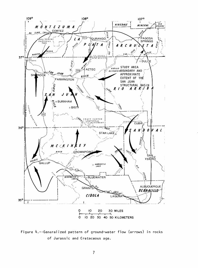
4. Map showing generalized pattern of ground-water flow(arrows) in rocks of Jurassic and Cretaceous age .......... 7

5-7. Maps showing outcrop area and hydraulic characteristics of the:

5. Entrada Sandstone ..................................... 96. Morrison Formation .................................... 117. Gallup Sandstone of the Mesaverde Group ............... 13

iv

Page

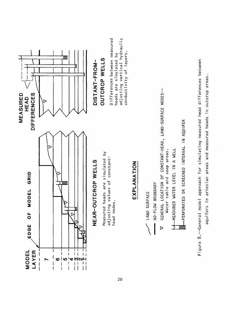
Figure 8. Diagram showing general model approach for simulatingmeasured head differences between aquifers in artesianareas and measured heads in outcrop areas................. 20

9. Map showing assigned hydraulic characteristics and model- derived flow rates for layer 1 (Entrada Sandstone) ....... 23

10. Map showing assigned hydraulic characteristics for layer 2(confining-beds) ......................................... 25

11-15. Maps showing assigned hydraulic characteristics and model- derived flow rates for:

11. Layer 3 (Westwater Canyon Member of MorrisonFormation) ......................................... 27

12. Layer 4 (confining-beds) ............................. 29

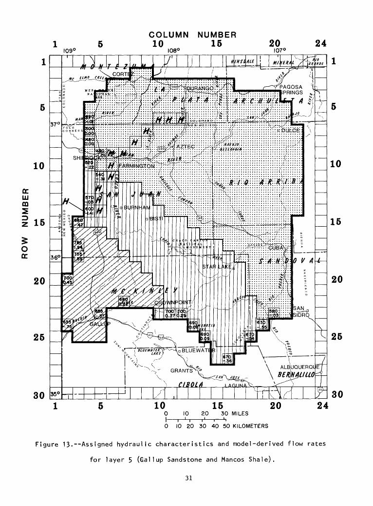
13. Layer 5 (Gallup Sandstone and Mancos Shale) .......... 31

14. Layer 6 (aquifers and confining beds in the middlepart of the Mesaverde Group) ....................... 33

15. Layer 7 (aquifers and confining beds in the upperpart of the Mesaverde Group) ....................... 35

16. Graph showing model-derived and measured heads for modellayers 1, 3, and 5 along section A-A ? ................... 37

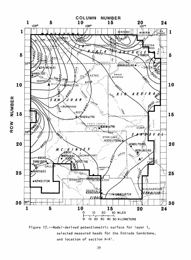
17. Map showing model-derived potentiometric surface for layer 1, selected measured heads for the Entrada Sandstone, and location of section A-A' ................. 39

18. Map showing model-derived potentiometric surface for layer 3, selected measured heads for the Morrison Formation (assumed to apply to the Westwater Canyon Member), and location of section A-A ? ................... 41

19. Map showing model-derived potentiometric surface for layer 5, selected measured heads for the Gallup Sandstone, and location of section A-A ? ................. 43

20. Graph showing correlation of model-derived heads tomeasured heads .......................................... 45

v

IllVSTRA T/M^-concluded

Page

Figure 21. Diagram showing results of sensitivity tests in terms of measured and model-derived heads at model row 17, column 13, and total flow at constant-head nodes ........ 50

22. Map showing constant-head nodes added to layer 7 toapproximate the overlying land-surface boundary ......... 52

TABLES

Table 1. Approximate density corrections to head data in the vicinityof Chaco Canyon National Monument ......................... 46

2. Flow rates at constant-head nodes for river drainage basinsand model layers .......................................... 48

VI

GLOSSARY

The following technical terms are used in this report:

Confining bed A confining bed is a body of "impermeable" material stratigraphically adjacent to one or more aquifers. In nature, however, hydraulic conductivity of confining beds may range from nearly zero to some value distinctly less than that of the aquifer.

Hydraulic head (L) The hydraulic head is the height above a standard datum of the surface of a column of water that can be supported by the static pressure at a given point. The standard datum in this report is sea level. Hydraulic head is referred to as head in this report.

Hydraulic conductivity (LT~1) Hydraulic conductivity is the characteristic of a medium that allows it to transmit, in unit time, a unit volume of ground water at the prevailing viscosity through a cross section of unit area, measured at right angles to the direction of flow, under a hydraulic gradient of unit change in head through unit length of flow.

Sea level Sea level is the term used in this report for the National Geodetic Vertical Datum of 1929, a geodetic datum derived from a general adjustment of the first-order level nets of both the United States and Canada, formerly called mean sea level.

Specific capacity (I/T~*) Specific capacity is the rate of discharge of water from a well divided by the drawdown of water level within the well.

Transnissivity (I, T~l) The transmissivity of an aquifer is the rate at which water of the prevailing viscosity is transmitted through a unit width of the aquifer under a unit hydraulic gradient. It is equal to the thickness of the aquifer multiplied by the hydra*ulic conductivity. (Conversely, the horizontal hydraulic conductivity in a model layer is the transmissivity of the aquifer that is represented divided by the thickness of the layer.) An approximation of transmissivity (in feet squared per day) can be obtained by multiplying the specific capacity (in gallons per minute per foot of drawdown) by 200.

vii

CONVERSION FACTORSMeasurements in this report are given in inch-pound units only. The following table contains factors for converting these units to metric units.

Multiply inch-pound unit

inchfootfoot per secondfoot squared per daycubic foot per secondacremilegallon per minutegallon per minute per foot

By_

25.400.3048.3048.0929.02832

4,0471.609.06309.20699

To obtain metric unit

millimeter meter

*

meter per second meter squared per day cubic meter per second square meter kilometer liter per second liter per second per meter

viii

ESTIMATES OF VERTICAL HYDRAULIC CONDUCTIVITY

AND REGIONAL GROUND-WATER FLOW RATES

IN ROCKS OF JURASSIC AND CRETACEOUS AGE,

SAN JUAN BASIN, NEW MEXICO AND COLORADO

by Peter F. Frenzel and Forest P. Lyford

ABSTRACTThe San Juan structural basin in northwestern New Mexico was modeled in

three dimensions using a finite-difference, steady-state model. The modeled space was divided into seven layers of square prisms that were 6 miles on a side in the horizontal directions. In the vertical direction, the layers of prisms ranged in thickness from 300 to 1,500 feet. The model included the geologic section between the base of the Entrada Sandstone and the middle of the Lewis Shale. Principal aquifers in this section are mostly confined and include the Entrada Sandstone, the Westwater Canyon Member of the Morrison Formation, and the Gallup Sandstone in the lower part of the Mesaverde Group.

Values for vertical hydraulic conductivities from 10""^ to 10""^ foot per second for the confining layers gave a good simulation of head differences between layers, but a sensitivity analysis indicated that these values could be between 10 and 100 times greater. The model-derived steady-state flow was about 30 cubic feet per second. About one-half of the flow was in the San Juan River drainage basin, about one-third in the Rio Grande drainage basin, and one-sixth in the Puerco River drainage basin.

INTRODUCTION

Purpose and Scope

The demand for water in the San Juan structural basin of northwestern New Mexico increases with the development of energy resources. Because the surface waters in this area are fully appropriated, much of the increase will need to be obtained from ground-water sources. In anticipation of continued increasing demands for water and attendant impacts on the ground-water and surface-water resources, a project was started during 1974 by the U.S. Geological Survey in cooperation with the New Mexico Bureau of Mines and Mineral Resources and the New Mexico State Engineer Office. The purposes of that project were to determine the general availability of ground water in the San Juan structural basin and to evaluate possible effects of ground-water development on ground-water and surface-water supplies.

The project has resulted in several reports including one by Stone and others (1983), which is the project's major report, and those by Lyford (1979) and by Lyford, Frenzel, and Stone (1980). This report is the final report to be prepared by the Geological Survey for the project.

A three-dimensional, digital-flow model with seven layers was constructed to approximate steady-state conditions during this part of the project. The primary purpose of the model was to provide estimates of leakage between aquifers and of total inflow and outflow through rocks of Jurassic and Cretaceous age.

Setting

The modeled area includes most of the San Juan structural basin in New Mexico and Colorado (fig. 1). Prominent geographical features around the perimeter of this area include the San Juan and La Plata Mountains in Colorado; the Carrizo Mountains, Chuska Mountains, and Defiance uplift along the New Mexico and Arizona border; the Zuni Mountains on the southwest, and the Rio Puerco fault belt and Nacimiento uplift on the east. Annual precipitation ranges from 6 inches near the central part of the area to more than 20 inches in mountainous parts. Population centers include Durango and Cortez in Colorado, and Farmington, Shiprock, Gallup, and Grants in New Mexico. Industrial developments include two large coal mines near Farmington that supply coal to nearby power plants; a large coal mine near Gallup; numerous uranium mines concentrated in the Laguna, Grants, and Gallup areas; oil and gas production; and the Navajo Indian Irrigation Project near Farmington, which eventually may include 110,000 acres of irrigated land. Many other uranium and coal mines are proposed.

CARRIZO MTS

, ,, STUDY AR */.f£m/*BOUNDARY

APPROXIMATE EXTENT IFARMINGTON

STRUCTURAL &\SI

EMBAYMENT

COLORADOStructural elements modified from Kelley, 1951 10 20 30 MILES

0 10 20 30 40 50 KILOMETERS

Figure 1. Location of the study area.

Acknowledgments

William J. Stone of the New Mexico Bureau of Mines and Mineral Resources, a principal investigator in the cooperative project, provided valuable information about the geologic framework of the study area. Many companies and consulting firms contributed aquifer-test data, as well as helpful discussions about ground-water resources, and allowed access to wells for water-level observations. The Navajo Nation and U.S. Bureau of Indian Affairs provided many well records and allowed access to wells. Glenn A. Hearne, hydrologist, U.S. Geological Survey, offered advice on the technical aspects of modeling and reviewed this report.

GEOHYDROtOGy OF TH£ MODELED AREA

A generalized geologic section of the San Juan Basin is shown in figure 2. The model emphasizes the interval between the base of the Jurassic Entrada Sandstone and the middle of the Cretaceous Lewis Shale. This interval has been divided into the seven model layers that will be discussed in the section "Steady-state model." The principal rock units in each model layer are shown in figure 3.

The major aquifers in the stratigraphic interval included in the model are the Entrada Sandstone and Westwater Canyon Member of the Morrison Formation of Jurassic age, and the Gallup Sandstone and some younger sandstones of the Mesaverde Group of Cretaceous age (figs. 2 and 3). Where these aquifers crop out, water is unconfined, but in most of the basin each aquifer is confined and separated from the others by shale beds.

Generally, the flow of water (fig. 4) in rocks of Jurassic and Cretaceous age is from recharge areas in the highlands around the edges of the basin toward streams that leave the basin to the northwest, southwest, and southeast. The rate of flow through the basin is small. Generally, discharges from the bedrock to the rivers are small, difficult to separate from flow derived from other sources, and, to date, have not been successfully measured by stream-gaging techniques.

The possible existence of vertical flow of water through confining beds is indicated by head differences of 100 feet between major aquifers, as measured in the area near Chaco Canyon National Monument (fig. 4). Springs are evidence of vertical flow in the Rio Puerco fault belt in the southeast and near the western end of the Hogback monocline in the northwest. Springs are associated with volcanic intrusives near the Cebolleta Mountains in the southeast and south of Shiprock in the northwest. Minor faults exist, especially between Crownpoint and Bluewater in the south, but it is not known if vertical ground-water flow is associated with these fractures.

MA/

VCO

S S

HA

LE^

POIN

T LO

OKOU

Tc

-

-10,0

00'-

I

0 5

10

20 M

ILE

S

I H

i i r-'

0 10

20

30

K

ILO

ME

TER

S

VE

RT

ICA

L

EX

AG

GE

RA

TIO

N

X 2

1

h - 8

000'

L -1

0,0

00'

Figure 2.

Gen

eralized ge

olog

ic section

of th

e San

Juan Ba

sin.

D

oUJ

u <h-UJ

c*

U

U

to

D Ok.u

Cliff House

Sandstone

Menefee Formation

Point Lookout Sandstone.«.». A .« . ». A .« .». A A .t.

CrevasseCanyonFormation Mancos

Shale(includes Dalton Sandstone and Dilco Coal ^(includes Mulatto;: Members) Jr. and Satan Tongues)

* ' *'*'

Gallup ^ij::: Mancos

Sandstone ^M Shale....

M a ri 'c b s S h a I e

Dakota Sandstone

.2 ot E

;: Brushy Basin Member

Westwater CanyonMember >- _* . ».j» ». ^

i; Recopture Member:::::::;:::::::Salt Wash Member-

Cow Springs SandstoneBluff SandstoneSummervilie FormationTodilto Limestone :*:

Entrada Sandstone

Layer 7,

1500 feet

thick

Layer 6,

1000 feet

thick

Layer 5,

700 feet

thick

Layer 4,

500 feet thick

Layer 3, 300 feet thick

Layer 2,

500 feet thick

Layer 1, 300 feet thick

NOTE: Shaded areas are defined as confining beds in the model.

Figure 3- Relation between geologic units and model layers.

37 Q

MONTEZVMA /

PAGOSA SPRINGS

STUDY AREAAND (

APPROXIMATE ( EXTENT OF THE* SAN JUAN { STRUCTURAL B.ASIN

RIO A R R\l B A

FARMiNGTON

. n BURNHAM

aBLUEWATER

GRAN

CtBOtA

0 10 20 30 MILESI i-H rj , h

0 10 20 30 40 50 KILOMETERS

Figure A.--GeneralIzed pattern of ground-water flow (arrows) In rocks

of Jurassic and Cretaceous age.

The following discussion is mainly from Lyford (1979), who described the general hydrology; Stone (1979), who described the lithology of measured sections; and Ridgley and others (1978), who summarized the stratigraphy of the San Juan Basin. The head, transmissivity, and specific-capacity data are taken from Stone and others (1983).

Aquifers

There are four major aquifers in the modeled interval. These aquifers are described in ascending order.

Entrada Sandstone

The Entrada Sandstone, present throughout the basin, is nearly 420 feet thick near the center of the basin (Ridgley and others, 1978). Stone (1979) noted a thickness of 236 feet or more at a site (T. 15 N. , R. 11 W.) between Crownpoint and Ambrosia Lake. The Entrada Sandstone consists of well-sorted, fine- to medium-grained sandstone with interbedded siltstone and mudstone. Transmissivity values range from less than 50 feet squared per day near the outcrops on the southern and western sides of the study area to about 400 feet squared per day near Chaco Canyon National Monument (J. W. Shomaker, consulting geologist, written commun., 1974). The water-level altitude in wells completed in the Entrada is about 90 feet lower than the water-level altitude in wells in the overlying Morrison Formation in the Chaco Canyon area (J. W. Shomaker, oral commun., 1977). Transmissivity and specific-capacity values are shown in figure 5. Selected head values for the Entrada Sandstone and other aquifers are reported, for convenience, in the part of the report where the model is described. Storage-coefficient values are not reported because they are not needed for a steady-state model.

EXPLANATION FOR FIGURE 5

OUTCROP OF ENTRADA SANDSTONE--(Dane and Bachman, 1965)

. 4e WELL-Upper number is transmissivity, in feet squared per day,0.02 e indicates estimated from specific capacity, ? indicates

calculations were made from incomplete data; lower numberis specific capacity, in gallons per minute per foot of draw down; Jcs indicates well also may be completed in Cow Springs Sandstone

109°

M 0 If T E Z V M A >/

, ZTEC STUDY AREA AZTEC rSfc ,mm/,BOUNDARY AND

! APPROXIMATE EXTENT OF SAN JUANSTRUCTURAL B,ASIN

RIO A K K\l

|FARMINGTON

QROWNPOINT

ALBUQUERQUE

CI SO LA LAGUNA

0 10 20 30 MILESI r-H r1 , ^

0 10 20 30 40 50 KILOMETERS

Figure 5. Outcrop area and hydraulic characteristics of the Entrada Sandstone,

Westwater Canyon Member of the Morrison Formation

The Westwater Canyon Member of the Morrison Formation (or its equivalents) is present throughout the area, ranges in thickness from 100 to 400 feet, and consists predominantly of sandstone and conglomeratic sandstone with minor siltstone and claystone. The more permeable material is in the southwestern part of the area. The transmissivity of the entire Morrison Formation ranges from less than 50 feet squared per day in the northeastern part of the area to about 500 feet squared per day in the south-central part (fig. 6). The Westwater Canyon Member is the most permeable unit in the Morrison Formation; therefore, transmissivity values measured by aquifer tests usually pertain to the Westwater Canyon Member.


\^£:-x\ OUTCROP OF MORRISON FORMATION ^""^iill? (Dane and Bachman, 1965)

APPROXIMATE BOUNDARY BETWEEN TRANSMISSIVITY ZONES

50-100 RANGE OF TRANSMISSIVITY, IN FEET SQUARED PER DAY

WELL Upper number is transmissivity, in feet squared per day, ? indicates calculations were made from incomplete data; lower number is specific capacity, in gallons per minute per foot of drawdown

NOTE: Transmissivity zones represent regional interpretations and do not necessarily fit individual control points.

10

109° 108°

T £ ICORTEZ

PAGOSA ' SPRINGS

STUDY AREA

AND rAPPROXIMATE EXTENT OF THE SAN JUAN / STRUCTURAL BASIN

ALB.UQUERQUE]

.^*

10I

20 30 MILES

0 10 20 30 40 50 KILOMETERS

Figure 6.--Outcrop area and hydraulic characteristics of the Morrison Formation

11

Gallup Sandstone of the Mesaverde Group

The Gallup Sandstone is the lowest unit in the Mesaverde Group. It is about 260 feet thick near Gallup but thins to the northeast where the main sandstone body pinches out into the Mancos Shale. The Gallup Sandstone is a complex sequence of sandstone, shale, and coal beds. Transmissivity values range from less than 100 feet squared per day near where the main body of the sandstone ends to 350 feet squared per day in the southwest, where it is the main source of water for the city of Gallup (fig. 7).


OUTCROP OF GALLUP SANDSTONE (Dane and Bachman, 1965)

WELL Upper number is transmissivity, in feet squared per day; ? indicates calculations were made from incomplete data; lower number is specific capacity, in gallons per minute per foot of drawdown; Kcd - well is also completed in Dalton Sandstone Member of the Crevasse Canyon Formation

APPROXIMATE BOUNDARY BETWEEN TRANSMISSIVITY ZONES

50-100 RANGE OF TRANSttlSSIVITY, IN FEET SQUARED PER DAY

NOTE: Transmissivity zones represent regional interpretations and do not necessarily fit individual control points

12

STUDY AREA *f«m/*BOUNDARY AND

APPROXIMATE , EXTENT OF THE SAN JUAN ( STRUCTURAL10 A R R\/ B A

S A N\9 0

ALBUQUERQUE

BEMMUUOGRAN

CISOtA35°

20 30 MILES

0 10 20 30 40 50KIIOMETERS

Figure 7.--Outcrop area and hydraulic characteristics of the Gallup Sandstone of

the Mesaverde Group.

13

Other aquifers in the Mesaverde Group

The principal water-yielding sandstones of the Mesaverde Group above the Gallup Sandstone are, in ascending order, the Dalton Sandstone Member of the Crevasse Canyon Formation, the Point Lookout Sandstone, sandstones of the Menefee Formation, and the Cliff House Sandstone.

The Dalton Sandstone Member of the Crevasse Canyon Formation crops out in the southern and southwestern parts of the area and intertongues north eastward with the Mancos Shale. At a site 10 miles northeast of Gallup (in sec. 2, T. 16 N., R. 17 W.), the Dalton is 270 feet thick and consists of mostly fine-grained, moderately sorted sandstone with intertonguing shale (Stone, 1979).

The Point Lookout Sandstone, present throughout the area, is about 120 feet thick in the southeastern part of the area, thickening to 380 feet in the northeastern part. It is mostly medium- to fine-grained sandstone with some shale.

The Menefee Formation, also present throughout the area, consists of fluvial sandstone, shale, and coal. From near Crownpoint to the northeast, its outcrop is a wedge that thickens to about 2,000 feet near the Chaco River. Farther to the northeast the formation thins and intertongues with the overlying Cliff House Sandstone.

The Cliff House Sandstone ranges in thickness from less than 100 feet in the northeastern part of the area to about 1,000 feet in a band from southeast to northwest across the middle of the area. It intertongues to the southwest with the underlying Menefee Formation and to the northeast with the overlying Lewis Shale. The Cliff House consists of medium- to fine-grained sandstone.

The transmissivity for the Mesaverde Group, excluding the Gallup Sandstone, ranges from less than 25 feet squared per day in the northeast to 100 feet squared per day in the southwest. Regional values of transmissivity are difficult to assign because of the discontinuous character of the sandstones.

Confining-bed sequences

The four principal aquifers lie between, and interfinger with, the five confining-bed sequences. The confining-bed sequences are described in ascending order.

14

Rocks directly underlying the Entrada Sandstone

Underlying the Entrada Sandstone are, in ascending order, the Chinle Formation and the Wingate Sandstone. The Chinle Formation is mostly mudstone and siltstone and ranges in thickness from 100 feet in the northeast to 1,500 feet in the southwest (Jobin, 1962, fig. 12). The Wingate Sandstone, present only in the west, thins eastward from the Chuska Mountains where it may be as much as 550 feet thick (Harshbarger and Repenning, 1954; Harshbarger, Repenning, and Irwin, 1957; and Ridgley and others, 1978). The more permeable upper part of the Wingate Sandstone is made up of fine- to very fine grained sandstone and "... will yield only small quantities of water to a well ..." (Harshbarger and Repenning, 1954).

Rocks between the Entrada Sandstone and the Westwater Canyon Member of the Morrison Formation

The confining-bed sequence between the Entrada Sandstone and the Westwater Canyon Member of the Morrison Formation includes, in ascending order, the Todilto Limestone, Summerville Formation, Bluff Sandstone, Cow Springs Sandstone, and the Salt Wash and Recapture Members of the Morrison Formation (fig. 3). The combined thickness of these rocks generally is about 500 feet.

Immediately overlying the Entrada Sandstone, the Todilto Limestone is present throughout the area. The thickest section is in the eastern one-half of the area where a gypsum/anhydrite facies in the upper part of the Todilto is as much as 100 feet thick. The presence of gypsum and anhydrite may indicate little interaquifer movement of water in the eastern one-half of the basin. The limestone facies is present throughout most of the area. It generally is in the lower part of the unit and is as much as 30 feet thick (Green and Pierson, 1977, p. 151).

The Summerville Formation, which overlies the Todilto, also is present in most of the area. The Summerville ranges in thickness from 10 to 60 feet and consists mostly of silty sandstone, sandy siltstone, and mudstone.

The Bluff Sandstone overlies the Summerville. Present mainly in the northwestern part of the area, the Bluff is about 375 feet thick in Utah and thins to the southeast. It is about 30 feet thick in the area between the Four Corners and the Chuska Mountains. It is fine- to medium-grained sandstone.

The Cow Springs Sandstone intertongues with the Bluff Sandstone. The Cow Springs is present only in the southwestern part of the area, is as much as 440 feet thick, and thins to the north and east. It consists of medium- to fine-grained sandstone.

15

The Salt Wash Member of the Morrison Formation overlies the Bluff Sandstone and intertongues with the overlying Recapture Member of the Morrison Formation. The Salt Wash is present in the northwestern part of the area, is as much as 300 feet thick, and consists of very fine grained sandstone, siltstone, and claystone. The Recapture Member of the Morrison Formation is present throughout the area, ranges in thickness from 125 to 300 feet, and is made up of fine-grained sandstone, siltstone, and mudstone.

Rocks between the Westwater Canyon Member of the Morrison Formation and the Gallup Sandstone of the Mesaverde Group

The confining-bed sequence between the Westwater Canyon Member of Morrison Formation and the Gallup Sandstone includes the Brushy Basin Member of the Morrison Formation, the Dakota Sandstone, and the lower part of the Mancos Shale (fig. 3).

The Brushy Basin Member of the Morrison Formation overlies and intertongues with the Westwater Canyon Member. The Brushy Basin is present throughout the area, except in the southwest where it has been removed by pre-Dakota erosion. It is greater than 400 feet thick in places, but generally is about 185 feet thick. Mostly, it is very fine grained sandstone and montlnorillonitic silty claystone. However, in the eastern and northeastern parts of the area, it includes the Jackpile sandstone (informal usage), which is coarser grained.

The Dakota Sandstone overlies the Brushy Basin and is as much as 350 feet thick. It is lenticular and consists of conglomeratic sandstone, carbonaceous shale, coal, and medium- to fine-grained sandstone. The lenticularity of the Dakota Sandstone is assumed to cause it to have a low regional transraissivity.

The Mancos Shale is mostly shale and siltstone with lesser amounts of limestone, sandstone, and bentonite. Between the Dakota and Gallup Sand stones, the lower part of the Mancos Shale ranges in thickness from about 500 to 1,000 feet (Molenaar, 1977). Toward the northeast, beyond the area of the main body of the Gallup Sandstone (fig. 7), the Mancos Shale is more than 2,000 feet thick. Although the Mancos Shale is considered to have fairly uniform hydraulic characteristics, parts of the Mancos were assigned to model layers 4, 5, and 6 (See fig. 3 and the section on "Model specifications").

16

Rocks between the Gallup Sandstone and other aquifers in the Mesaverde Group

Throughout most of its area, the Gallup Sandstone is separated from the other aquifers in the Mesaverde Group (fig. 2) by as much as 1,000 feet of Mancos Shale. However, in the south, the Gallup Sandstone is overlain by the Crevasse Canyon Formation of the Mesaverde Group, which contains intertonguing sandstone and shale deposits. In this area, the Gallup Sandstone is separated from the Dalton Sandstone Member of the Crevasse Canyon Formation by the Dilco Coal Member of the Crevasse Canyon Formation (Molenaar, 1977). The Dilco Coal Member contains about 25 percent medium- to fine-grained sandstone and 75 percent carbonaceous shale in a 176-foot thickness at a site due west of Ambrosia Lake and due north of Bluewater (T. 14 N., R. 11 W.) (Stone, 1979).

Rocks above the Mesaverde Group

The Lewis Shale overlies the Cliff House Sandstone in the upper part of the Mesaverde Group. The Lewis Shale increases in thickness from where it pinches out near Burnham to about 2,600 feet in the northeast. It consists predominantly of gray-to-black shale with thin beds of sandstone and limestone.

Hydraulic characteristics of the confining beds

The hydraulic characteristics of the confining beds are largely unknown. The following reported test data may indicate possible vertical hydraulic conductivity values for the rocks involved.

J. W. Shomaker (written commun., 1978) tested the permeability of the Summerville Formation at a well 6 miles east of Chaco Canyon National Monument. Core analyses using an 8,000 milligrams-per-liter solution of sodium chloride as the testing fluid gave permeabilities ranging from 3.9 x 10~6 to 6.1 x 10~5 millidarcy (1.1 x 10~13 to 1.7 x 10~12 foot per second at 60° F). The tested section was described as a fine- to very fine grained, well to moderately indurated sandstone with a porosity ranging from 1.6 to 6.3 percent. Bredehoeft and Hanshaw (1968, p. 1,101) reported hydraulic conductivities for compacted shale ranging from 2.0 x lO"-"- 2 to 6.0 x 10~10 centimeter per second (6.6 x 10~14 to 2.0 x 10"11 foot per second). Young, Low, and McLatchie (1964, p. 4,239-4,240) reported that for some Cretaceous rocks of western Canada, siltstones and sandstones have permeabilities measured perpendicular to the bedding ranging from 10~' to 10~4 millidarcy (2.8 x 10~15 to 2.8 x 10~12 foot per second at 60° F).

17

STEADY-STATE MODEL

General procedure

The three-dimensional flow model was used to provide estimates of the steady-state rate of flow through the rocks in the geologic section previously described and estimates of the vertical hydraulic conductivities of the major confining-bed sequences in this geologic section.

The computer program used in this study is described in Posson and others (1980). The program uses the strongly implicit procedure of Stone (1968) to solve the finite-difference approximation of the following partial differential equation of ground-water flow in three dimensions:

d ah d ah a ah ah Kx + Ky + Kz = S s + W (x,y,z,t)ax ax ay ay az az at

where

Kx , Ky, Kz are the hydraulic conductivities in the x, y, and zdirections

h is the head (L) above a standard datum;

S s is the specific storage (L~"l) (Specific storagewas zero for this steady-state application); and

W (x, y, z, t) is the volumetric flux per unit volume (T~"l) (suchas discharge from a well). The W term was zero in this model.

The modeling procedure consisted of three steps: (1) Specification of the steady-state model; (2) calibration of the steady-state model; and (3) a sensitivity analysis of the calibrated model. The sensitivity analysis was designed to assess the accuracy of the model-derived values of vertical hydraulic conductivity.

Specification of the steady-state model mainly consisted of three steps:(1) Assigning layers of the model to the aquifers and confining beds;(2) defining the recharge-discharge boundary as a constant-head surface that was equal to the altitude of the land surface; and (3) assigning values of hydraulic conductivity.

In general, the calibration procedure attempted to minimize differences between the measured and model-derived potentiometric surfaces by adjusting aquifer and confining-bed properties and boundary conditions in the model.

18

The major effort in the calibration was to adjust vertical hydraulic conductivity values until the measured head differences between aquifers were simulated for an area (right side of fig. 8) located relatively distant horizontally from the land-surface boundary (outcrop area left side of fig. 8). Heads at locations near the land-surface boundary (left side of fig. 8) were simulated by adjusting the values of the constant-head nodes in the outcrop area.

The sensitivity analysis consisted of four basic steps. First, in view of the data available, a range of "reasonable" values for each hydraulic characteristic was determined. Second, the calibrated model was altered, setting the value of each hydraulic characteristic (except vertical hydraulic conductivity), one at a time, at the maximum value of its range and then at the minimum value. Third, vertical hydraulic conductivity was investigated, narrowing the range of possible values. Fourth (referring back to the second step) the effects of possible errors in certain hydraulic characteristics on estimates of vertical hydraulic conductivity were investigated.

Model specifications

The finite-difference scheme requires that the modeled space be divided into layers of prisms. In the vertical direction, seven layers of prisms approximated the geologic units between the base of the Entrada Sandstone and the top of the Mesaverde Group (fig. 3). The layers ranged in thickness from 300 to 1,500 feet. Each layer consisted of 720 prisms, 24 prisms to a row in the east-west direction and 30 prisms to a column in the north-south direction. Each prism was 6 miles on a side in each horizontal direction. The center point of a prism is called a node.

Boundaries

Although each layer of the model contained 720 prisms, not all of these prisms were "active"; that is, not all prisms were defined as having water movement. The number of active prisms ranged from 317 in layer 7 to 528 in layer 2.

In each layer, the inactive prisms (those with zero hydraulic conductivity) form a no-flow boundary around the active prisms. This boundary is also referred to as the "extent of layer" in figures 9-15. In the northwest, where the deeper geologic units extend slightly beyond the modeled area, constant-head nodes approximate flow across the "extent of layer" boundary. In addition, a no-flow boundary was defined at the top of layer 7 and at the bottom of layer 1 (fig. 3). All non-zero flow rates were model derived and occurred at constant-head nodes.

19

MO

DE

L

LA

YE

RE

DG

E

OF

M

OD

EL

G

RID

ME

AS

UR

ED

HE

AD

D

IFF

ER

EN

CE

S

NE

AR

-OU

TC

RO

P

WE

LL

S

Meas

ured he

ads

are

simulated

by

adjusting

values of constant-

head nodes.

EX

PL

AN

AT

ION

/

DIS

TA

NT

-FR

OM

-

OU

TC

RO

P

WE

LL

S

Diff

eren

ces

between

measured

head

s ar

e simulated

by

adjusting

vertical hydraulic

conductivity of la

yers

.

_X~ LA

ND SU

RFAC

E

NO-FLOW

BOUN

DARY

V

GENERAL

LOCATION OF

CONSTANT-HEAD, LAND-SURFACE NODES--

Water

tabl

e and

seep ar

eas.

-MEA

SURE

D WATER

LEVE

L IN A

WELL

-PER

FORA

TED

OR SC

REEN

ED INTERVAL IN

AQUIFER

Figure 8.

--Ge

nera

l mo

del

appr

oach

for

simu

lati

ng me

asur

ed he

ad differences

between

aqui

fers in

ar

tesi

an ar

eas

and;

me

asur

ed he

ads

in outcrop

area

s.

A constant-head boundary immediately inside the no-flow boundary was specified for each layer in outcrop areas except layer 2. Layer 2 was excluded because of its relatively narrow outcrop and low horizontal hydraulic conductivity with respect to overlying and underlying layers. The heads for these constant-head nodes initially were selected from streambed altitudes and later adjusted during calibration. In addition, several constant-head nodes were specified in layers 1 and 3 along the northwestern edge of the modeled area near Four Corners to approximate underflow from the modeled area into Utah, which is outside the no-flow boundary. The head values in these nodes were selected from streambed altitudes along the San Juan River and its tributaries in Utah.

Aquifers

The distribution of horizontal hydraulic conductivity values in each layer of the model generally is patterned after the transmissivity distribution for the corresponding aquifer because hydraulic conductivity is equal to transmissivity divided by aquifer thickness. The vertical hydraulic conductivity values were derived during model calibration and are explained in the section "Adjustments and constraints on adjustment."

The distribution of horizontal hydraulic conductivity in layer 1 (representing the Entrada Sandstone) is shown in figure 9. A comparison of the three peripheral transmissivity values with the value near Bisti (fig* 5) suggests a larger horizontal hydraulic conductivity toward the center of the basin, but the distribution needs to be estimated without supporting geologic data. The effect of temperature on hydraulic conductivity provides a rationale for the distribution. Temperature increases with depth; the effect of higher temperature, all other things being equal, would result in an increase in hydraulic conductivity where an aquifer is deeply buried. Therefore, the general distribution of hydraulic conductivity (fig. 9) was determined on the basis of depth of burial. Temperature gradients were reported by Reiter and others (1975). The gradients and depth of burial would support a threefold increase in the zone of larger hydraulic conductivity compared to the zone of smaller hydraulic conductivity shown in figure 9. In contrast, a much larger increase (tenfold or more) is indicated by the somewhat questionable data in figure 5. Thus, the final values used (fig. 9) reflect an intermediate sevenfold increase.

The distribution of horizontal hydraulic conductivity in layer 3 (fig. 11), representing the Westwater Canyon Member of the Morrison Formation, generally is patterned after the transmissivity distribution in figure 6. The largest transmissivity values in figure 6, in the southeastern part of the area, are not thought to be regionally significant.

The values and distribution of horizontal hydraulic conductivity in layer 5 (fig. 13), representing the Gallup Sandstone, are patterned after the values and distribution of transmissivity in figure 7.

21

The distribution of horizontal hydraulic conductivity in layers 6 and 7 (figs. 14 and 15) are patterned after the values and distribution shown in figure 8 of Lyford (1979) for part of the Mesaverde Group. Layers 6 and 7 represent parts of the Mancos Shale, Mesaverde Group, and Lewis Shale. The values of horizontal hydraulic conductivity of layers 6 and 7 are not important to this particular model because of the coincidence of these layers with much of the area of the constant-head land-surface boundary. Thus, the major effect of these two layers on this model is that of a confining bed where vertical hydraulic conductivity dominates flow.

Confining beds

The values of horizontal hydraulic conductivity (10"~° and 10~' foot per second) for confining beds of layers 2, 4, and parts of 5 and 6 (figs. 10 and 12-14) were estimated from published descriptions of the geology. The geologic units represented by these layers are shown in figure 3. The effect of errors in the horizontal hydraulic conductivity of confining beds was considered in the sensitivity analysis. Vertical hydraulic conductivity values for confining beds were determined during calibration.


LAYER THICKNESS IS 300 FEET

NO-FLOW BOUNDARY Extent of layer

NODE WITH Kz = 5 x 10'9 , NEAR HOGBACK MONOCLINE

CONSTANT-HEAD NODE Top number is altitude, in feet, divided by 10; bottom number is flow rate,in cubic feet per second, positive value Indicates inflow; negative, outflow

HYDROLOGIC CHARACTERISTICS

H7800.27

T - 20, Kxy = 7.7 x 10'7 , Kz = 1.5 x 10'10

T - 150, Kxy = 5.8 x 10~6 , Kz - 1.2 x 10'9

where: T » Transmissivity, in feet squared per day

Kxy » Horizontal hydraulic conductivity, In feet per second

Kz Vertical hydraulic conductivity, In feet per second

22

109°

COLUMN NUMBER 10 15 24

OC UJ CD

O QC

:::S:^^^^

3024

0 10 20 30 40 50 KILOMETERS

Figure 9."Assigned hydraulic characteristics and model-derived flow

rates for layer 1 (Entrada Sandstone).

23




NODE WITH Kz = 5 x NT9 , NEAR HOGBACK MONOCLINE


T - 0.43, Kxy - 1 x 10~8, Kz = 1 x 10~12

T - 4.3, Kxy = 1 x 10~7, Kz - 1 x 10""


Kxy « Horizontal hydraulic conductivity, In feet per second

Kz « Vertical hydraulic conductivity, in feet per second

109°

COLUMN NUMBER 10 15

108°24

::::::::: :::::::-: :: x;::: ::::: :::: ::: *:: : :>:........................... -X-...........v^t^j ............ <ji.. ri. .*» . i*i

^LBUQUERQl E

1520 30 MILES

25

30

0 10 20 30 40 50 KILOMETERS

Figure 10. Assigned hydraulic characteristics for layer 2 (confining beds).

25

30

H630 -.20




NODE WITH Kz - 5 x 1CT9 , NEAR HOGBACK MONOCLINE

CONSTANT-HEAD NODE Top number Is altitude, In feet, divided by 10; bottom number is flow rate,in cubic feet per second, positive value indicates inflow; negative, outflow


T - 25, Kxy - 9-6 x 10'7 , Kz - 9-6 x 10'11

1 T - 100, Kxy - 3-9 x 10'6 , Kz - 3-9 x 10HO

T - 200, Kxy - 7.7 x 10"6 , Kz - 7.7 x 10'10

T - 250, Kxy - 9.6 x 10"6 , Kz - 9.6 x 10' 10

where: T - Transmissivity, in feet squared per day

Kxy - Horizontal hydraulic conductivity, in feet per second

Kz - Vertical hydraulic conductivity, in feet per second

26

109°

COLUMN NUMBER 10 15

108°20107°

24

3024

i r 0 10 20 30 40 50 KILOMETERS

Figure 11. Assigned hydraulic characteristics and model-derived flow rates

for layer 3 (Westwater Canyon Member of Morrison Formation).

27

H7800.01




NODE WITH Kz 5 x 1CT9 , NEAR HOGBACK MONOCLINE

CONSTANT-HEAD NODE Top number is altitude, in feet, divided by 10; bottom number is flow rate,in cubic feet per second, positive value indicates inflow; negative, outflow


T - Transmissivity, in feet squared per day


Kz « Vertical hydraulic conductivity, In feet per second

28

109°

COLUMN NUMBER 10 15

108°24

OC LU ffl5ID

O GC

T *0.43

Kz =1 x

^f-t ,_CROWNPOINT

0 10 20 30 40 50 KILOMETERS

Figure 12.--Assigned hydraulic characteristics and model-derived flow

rates for layer k (confining beds).

29

H

490-.01




NODE WITH Kz - 5 x TO'9 , NEAR HOGBACK MONOCLINE



T = 0.6, Kxy - 1 x 10'8 , Kz = 1 x 10' 12

T - 100, Kxy - 1.6 x 10'6 , Kz = 1.6 x 10*'°

T « 200, Kxy = 3.3 x 10'6 , Kz » 3.3 x 10"'°


Kxy » Horizontal hydraulic conductivity, in feet per second

Kz Vertical hydraulic conductivity, in feet per second

30


107°24

OC

QQ5ID

oDC

^Jfi*:::::::: A $mmmm.7. ......k_.^»J./r...C....,AX;....?...Hi.77..?...*?.../j£...l.. ,«f.?\..L,..«..v.p* W*WH| rf ^

fmiMT/jnr^HaBLUEWATE R

ItXNAUUA

30

1015 20

20 30 MILES

0 10 20 30 40 50 KILOMETERS


for layer 5 (Gall up Sandstone and Mancos Shale).

31

H

mmm




NODE WITH Kz - 5 x 10'9 , NEAR HOGBACK MONOCLINE



T - 0.86, Kxy - 1 x 10~8, Kz - 1 x 10~ 12

7200.00

T

where:

130, Kxy - 1.2 x 10~6, Kz - 1.2 x 10~'°

T * Transmissivity, in feet squared per day


Kz * Vertical hydraulic conductivity, In feet per second

32

COLUMN NUMBER 10 15

rPAGGSA 'I

^xxt^xT^x^^xTx:^^I 1 II ' " I 1 M ' " " f t" " ' V I ' " '"'' ' I" 's ' ' ' T-~-i^-r ."/.'.','. . .'. }.'.ft. '/I ,)9f.'

15 2020 30 MILES

25

30 3024

10 20 30 40 50 KILOMETERS

Figure 1^.--Assigned hydraulic characteristics and model-derived flow rates

for layer 6 (aquifers and confining beds in the middle part of

the Mesaverde Group).

33

H7200.36




NODE WITH Kz - 5 x 10'9 , NEAR HOGBACK MONOCLINE



T « Transmissivity, in feet squared per day

Kxy » Horizontal hydraulic conductivity, in feet per second

Kz « Vertical hydraulic conductivity, in feet per second

109°

COLUMN NUMBER 10 15

108°24

3024



for layer 7 (aquifers and confining beds in the upper part of the

Mesaverde Group).

35

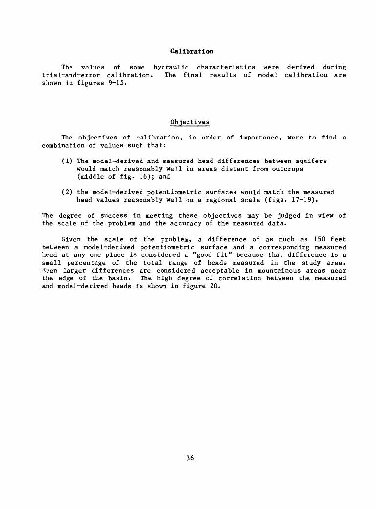
Calibration

The values of some hydraulic characteristics were derived during trial-and-error calibration. The final results of model calibration are shown in figures 9-15.

Objectives

The objectives of calibration, in order of importance, were to find a combination of values such that:

(1) The model-derived and measured head differences between aquifers would match reasonably well in areas distant from outcrops (middle of fig. 16); and

(2) the model-derived potentiometric surfaces would match the measured head values reasonably well on a regional scale (figs. 17-19).

The degree of success in meeting these objectives may be judged in view of the scale of the problem and the accuracy of the measured data.

Given the scale of the problem, a difference of as much as 150 feet between a model-derived potentiometric surface and a corresponding measured head at any one place is considered a "good fit" because that difference is a small percentage of the total range of heads measured in the study area. Even larger differences are considered acceptable in mountainous areas near the edge of the basin. The high degree of correlation between the measured and model-derived heads is shown in figure 20.

36

I III III I I ICHACO CANYON

NATIONAL MONUMENT

EXPLANATION

MEASURED HEADS

X Entrada SandstoneWestwater Canyon Member of the

Morrison Formation

Gall up Sandstone

jb May also be completed in other members of the Morrison Formation and Bluff Sandstone

MODEL-DERIVED HEADS (curves)

(Entrada Sandstone) (Westwater Canyon Member of the Morrison Formation)

5 - Layer 5 (Gall up Sandstone)

1 - Layer 1 3 ~ Layer 3


NODE LOCATION (ROW COLUMN)

Figure 16.--Model-derived and measured heads for model layers

1, 3, and 5 along section A-A 1 .

37


<6868(63)RD DRILL-STEM TEST

REPORTED (Guyton and Associates, 1978)

YEAR 1963

OF WATER-LEVEL MEASUREMENT,

-68OO-- WATER-LEVEL CONTOUR FOR MODEL-DERIVED POTENTIOMETRIC SURFACE Contour interval 200 feet. Datum is sea level


<A' SECTION

NOTE;

WATER-LEVEL ALTITUDE, IN FEET ABOVE SEA LEVEL "a" indicates altitude is corrected for density

WELL

Contours may not fit control points because the model-derived potentiometric surface was developed primarily by matching head differences between aquifers and second arily by matching measured heads (see "Calibration").

38

109°

COLUMN NUMBER 10 15

108° 24

30 30

0 10 20 30 40 50 KILOMETERS

Figure 17- Model-derived potentiometric surface for layer 1,

selected measured heads for the Entrada Sandstone,

and location of section A-A 1 .

39


5a(32)Kd WELL ALSO OBTAINS WATER FROM DAKOTA SANDSTONE

Jb WELL ALSO OBTAINS WATER FROM BLUFF SANDSTONE

WELL ALSO OBTAINS WATER FROM SUMMERVILLE FORMATION

YEAR OF WATER-LEVEL MEASUREMENT, 1932

WATER-LEVEL ALTITUDE, IN FEET ABOVE SEA LEVEL "a" indicates altitude is corrected for density

-WELL

V6360 HEAD, IN FEET ABOVE SEA LEVEL

\ SPRING OR RIVER

"6600 WATER-LEVEL CONTOUR FOR MODEL-DERIVED POTENTIOMETRIC SURFACE Contour interval 200 feet. Datum is sea level.


SECTION

NOTE: Contours may not fit control points because the model-derived potentiometrlc surface was developed primarily by matching head differences between aquifers and secondarily by matching measured heads (see "Calibration").

109°


30 3015 20

20 30 MILES

0 10 20 30 40 50 KILOMETERS

Figure 18.--Model-derived potentiometric surface for layer 3, selected

measured heads for the Morrison Formation (assumed to apply to

the Westwater Canyon Member), and location of section A-A 1 .

41

66l6o(72)


-YEAR OF WATER-LEVEL MEASUREMENT, 6600 WATER-LEVEL CONTOUR FOR MODEL-DERIVED 1972 POTENTIOMETR 1C SURFACE Contour intervalWATER-LEVEL ALTITUDE, IN FEET 20° feet ' Datum ls Sea leveK

ABOVE SEA LEVEL "a" indicates altitude is corrected for density

WELL

<? 6680 HEAD, IN FEET ABOVE SEA LEVEL

\ SPRING OR RIVER


A* SECTION

NOTE: Contours may not fit control points because the model-derived potentiometric surface was developed primarily by matching head differences between aquifers and secondarily by matching measured heads (see "Calibration")*

109°

COLUMN NUMBER 10 15

108°24

30 30

1015

20 30 MILES

0 10 20 30 40 50 KILOMETERS

Figure 19.--Model-derived potentiometric surface for layer 5, selected

measured heads for the Gall up Sandstone, and location of

section A-A 1 .

43

The accuracy of the measured-head data pertains to how well the data represent true steady-state conditions in the ground-water system. It was assumed that the ground-water system was at steady state before any pumping began, so the data were selected to best represent prepumping conditions. Errors due to short-term pumping, seasonal effects, and density effects could be as much as several tens of feet. Throughout most of the study area, errors of this magnitude are not significant with respect to the scale of the problem. However, in the area near Chaco Canyon, where the differences in head between aquifers were critical to this modeling, approach, the head data were corrected as much as possible for the density effects of temperature and salinity. The data and results of these corrections are shown in table 1. The assumptions and methods for making density corrections are described in the following paragraph.

The length of the water column within an aquifer was assumed to be insignificant because it generally was less than 10 percent of the total column length. Thus, the water column (B in table 1) in each instance extended from the top of the aquifer to the pressure gage for flowing wells or to the water level in the one nonflowing well. A correction for salinity was calculated by taking the specific gravity at 68° Fahrenheit (A) minus 1 times the length of the water column (B). Thus, the correction due to salinity was (A-l)B. An average temperature (Tavg) was estimated by assuming that, at the time of water-level measurement, the water column had cooled from the measured temperature (T) throughout the entire water column to a temperature half-way between T and the ambient rock temperature. The ambient rock temperature was assumed to vary linearly from 60° Fahrenheit at the top of the water column near land surface to T at the bottom of the water column. That is, the temperature of the water column at the time of water-level measurement was assumed to vary linearly from a value of T - (T-60)/2 at the top of the column to T at the bottom for an average (Tavg) of T - (T-60)/4. A specific gravity was calculated by dividing the density of pure water at the average temperature (C) by the density of pure water at 68°. From this, a temperature correction was calculated, (C-l)B, for each water column. The salinity and temperature corrections were added to the measured water-level altitude to obtain approximate corrected heads.

MEAS

URED

HEADS,

IN HU

NDRE

DS OF FE

ET AB

OVE

SEA

LEVE

L

Ul

ID C -\

(D K>

O I I O O -t -\

(D O

Q.

(D I 0.

(D (D

Q.

0)

QJ

Q.

0)

Q. 0) QJ Q.

O O c?

m CX3 O

Table 1.

App

roxi

mate

den

sity

cor

rect

ions

to he

ad data in the

vicinity of

Chaco Canyon Na

tion

al Honument

Diss

olve

d-

soli

ds

Appr

ox-

conc

en-

Imat

e tr

atio

n specific

in mil

li-

grav

ity

gram

s Reported

at 6

8°LO

CATI

ONLaye

r

1 1 3 3 3 3 5

Row 15 17 15 15 17 19 18

Column 9 13 9 9 13 16 13

per

lite

r

15,000

10,6

30 925

4,50

0

3,60

0

2,74

0

1,77

5

spec

ific

Fahren-

gravity

heit (A)

1.0144

1.01

44

1.00

7 1.

007

1.00

09

1.0045

1.0036

1.0027

1.0018

Corr

ec-

Leng

th

tion

of

fo

r water

sali

n-

colu

mn,

ity,

in

in f

eet

feet

(B)

5,78

8

5,36

1

5,00

0

5,043

4,617

4,58

5

3,00

0

[(A-l) B]

83 38 4 23 17 12 5

Approx

imat

e Te

mper

- av

erag

e ature

temp

er-

at the

ature

bott

om

of t

he

of the

water

*Spe

cifi

c water

column,

in gr

avit

y co

lumn

, in

de

gree

s of p

ure

degr

ees

Fahr

en-

water

Fahren

heit (T

)

141(

?)

144

142

140

134

149

100

heit

(Tav

g)

121

123

122

120

116

127

90

at Tavg

(C)

0.99027

.989

37

.989

819

.990

27

.991151

.988436

.996

816

Corr

ec

tion

for

temp

er

ature

in feet

[(C-l)B]

-56

-57

-51

^9

-41

-53

-10

Tota

l co

rrec

ti

on,

in f

eet

27(?

)

-19

-47

-26

-24

-41 -5

Wate

r-

level

alti

tude

,in

fee

t

6,3%

6,39

7

6,448

6,47

2

6,50

9

6,45

2

6,620

Head

,in

feet

6,42

3

6,378

6,40

1

6,44

6

6,48

5

6,41

1

6,615

*Density o

f pure water a

t th

e av

erag

e te

mper

atur

e di

vide

d by

the

density o

f pure water a

t 68°

Fahrenheit

Adjustments and constraints on adjustment

Boundaries. During calibration, some of the constant-head values were respecified to correspond better with measured heads in or near outcrop areas. Where respecified, values of constant-head nodes that simulated inflow (recharge) to the model were constrained to be equal to or less than the land-surface altitude. Conversely, in outflow (discharge) areas, values were constrained to be equal to or greater than the altitude of the land surface.

Aquifers. The horizontal hydraulic conduct'ivities in aquifer layers were kept approximately within ranges consistent with the transmissivity ranges shown in figures 5-7. The vertical hydraulic conductivity in the area along the western end of the Hogback monocline (fig. 9-15) was not constrained. It was adjusted to simulate the water-level altitudes in the vicinity south and west of Shiprock. In the rest of the modeled area, for convenience, the vertical conductivity was a multiple of the horizontal conductivity; for simplicity, the ratio of vertical to horizontal conductivity for the aquifers was assumed to be about the same as the ratio for the confining beds because both the aquifers and confining beds consist of thick sequences of sandstones and relatively impermeable shales.

Confining beds. Horizontal hydraulic conductivity in the confining beds was not adjusted during calibration based on the assumption that greater horizontal hydraulic conductivity in the aquifers would dominate the horizontal flow of the system. (The effect of horizontal hydraulic conductivity in the confining-bed sequences was tested in the sensitivity analysis.) Vertical hydraulic conductivities in the confining beds were not constrained.

Model-derived flows

The model-derived rate of flow through the structural basin was about 30 cubic feet per second; the total flow is arranged in table 2 by drainage basin and by layer. (All flows occur at constant-head, land-surface boundaries.) In table 2, the inflow is the recharge to the modeled system at constant-head nodes, and the outflow is the .discharge at constant-head nodes. Approximately one-half of the total inflow and outflow took place in the San Juan River drainage basin, one-third took place in the Rio Grande drainage basin, and one-sixth took place in the Puerco River drainage basin. The drainage basins and flows at individual constant-head nodes are indicated in figures 9-15. Inflow equals outflow for the system as a whole. The general direction of flow through the model has an upward component although the hydraulic gradient implies downward flow in the central part of section A-A1 (fig. 16) between layers 5 and 1. Upward flow is implied between layers 5 and 7 (figs. 15 and 19). The general directions of horizontal flows indicated by the model-derived heads are similar to those shown in figure 4.

47

Table 2. Flow rates at constant head nodes for river drainage basins and model layers

[All flow rates are given in cubic feet per second. Inflows are positive and outflows are negative. Total inflow = total outflow about 30 cubic feet per second.]

Model layers

Drainage basin

San Juan River

Rio Grande

Puerco River

Total rate by layer

1

2.66 -.54

.34 -.55

.25 -.16

3.25 -1.25

2

0 0

0 0

0 0

0 0

3

2.80 -1.97

2.21 -1.72

1.42 -1.04

6.43 -4.73

4 5

0.03 1.94 -.02 -2.43

.02 .73 0 -.98

0 2.36 0 -1.12

0.05 5.03 -.02 -4.53

6

0.30 -3.01

2.63 -1.67

.99 -.66

3.92 -5.34

7

6.68 -9.99

2.66 -2.49

.35 0

9.69 -12.48

Total rate by drainage basin

14.41 -17.96

8.59 -7.41

5.37 -2.98

28.37 -28.35

Sum of totals by layer 2.00 0 1.70 0.03 0.50 -1.42 -2.79

48

Sensitivity analysis

The objectives of the sensitivity analysis were to determine plausible ranges of vertical hydraulic conductivities and of flow through the basin. For the sensitivity tests, selected hydraulic characteristics were varied within ranges that were judged to be reasonable on the basis of the available geologic and hydrologic data. An example of the sensitivity test at one location is shown in figure 21.

Measured heads are shown in figure 21 for the Entrada Sandstone, Westwater Canyon Member of the Morrison Formation, and Gallup Sandstone at the location of model row 17, column 13. They are the lines labeled Je, Jmw, and Kg. Also shown are heads from the calibrated model at the same location for layers 1, 3, and 5 (lines labeled 1, 3 and 5). The lines labeled A, B, and C indicate the heads calculated by the model when each of the noted characteristics was changed. A flow rate that may be compared with the total flow of table 2 (30 cubic feet per second) is shown for each change. The location of row 17, column 13 was selected because the model was more sensitive to hydraulic characteristics (especially vertical hydraulic conductivity) at that location than at other locations where measured heads exist. In most of the other locations, the model-derived heads were more sensitive to the head values in the constant-head boundary than to any other characteristic. As stated previously, primary emphasis was given to matching head differences rather than actual heads.

In the following discussion, the heads derived from the calibrated model are referred to by their layer number (1, 3, or 5). The heads that result from the sensitivity test in question are referred to by letter (A, B, and C for layers 1, 3, and 5, respectively).

Three of the questions addressed in the evaluation of effects of each change shown in figure 21 are: (1) What is the overall effect in qualitative terms; (2) do any of the model-derived heads A, B, or C match the corresponding measured heads better than the heads 1, 3, or 5, respectively; and (3) how do the differences between heads A, B, and C compare with the differences between heads 1, 3, and 5 and between the measured heads?

Horizontal hydraulic conductivity

Changes to horizontal hydraulic conductivity in layer 1 generally had great effect, but the changes did not improve the match between model-derived and measured heads. For example, when one value of hydraulic conductivity was used uniformly throughout the whole layer, the differences between heads A and B was about zero, and both heads were too high when compared to the measured heads for the Entrada and Westwater.

49

Jmw MEASURED HEADS IN THE GEOLOGIC FORMATION

DERIVED HEADS IN LAYERS 1, 3, AND 5'

OF THE CALIBRATED MODEL,

OF THE MODEL WITH THE FOLLOWING CHANGES:

K of layer 1 X 5

K of layer 1 X 0.2

Uniform K in layer 1

K of layers 2 and 4 X 50 (I)

K of layer 3X2

K of layer 3 X 0.5

K of layer 5 X 2

K of layer 5 X 0.5

K of layer 6 and 7 X 5

Overlying land surfacein layer 7 (H)

K 1 of Hogback monocline(all layers) X 2 (m)

K 1 of Hogback monocline(all layers) X 0.5

K 1 of al1 layers* X 0.001

K 1 of al1 layers* X 0.1

K 1 of a 11 layers* X 10

K 1 of al1 layers* X 100

K 1 of layers 1-4* X 10

K 1 of layers 1-4* X 100 (H)

I and ESZ combined

El and EEC combined

63 64 65 66 67 68

HEAD, IN HUNDREDS OF FEET ABOVE SEA LEVEL

-^ LEI and DZ" combined

FLOW(IN CUBIC FEET PER SECOND)

37

26

33

31

25

33

26

84

37

29

2827

27

34

56

30

43

50

52

43

Je = Entrada Sandstone, Jmw = Westwater Canyon Member of the Morrison Formation, Kg - Gallup Sandstone, K - horizontal hydraulic conductivity, in feet per second, K 1 = vertical hydraulic conductivity, in feet per second (* except in Hogback monocline area).

Figure 21.--Results of sensitivity tests in terms of measured and model-

derived heads at model row 17, column 13, and total flow

at constant-head nodes.

50

Multiplying the horizontal hydraulic conductivities of layers 2 and 4 by 50 caused a great effect. The values of A, B, and C matched the measured heads better than 1, 3, and 5; but the differences between A, B, and C were greater than between 1, 3, and 5, as well as between the measured heads.

Most of the changes of horizontal hydraulic conductivity in layers 3, 5, 6, and 7 had relatively little effect (as compared to changes of other hydraulic characteristics). An exception is the case in which the horizontal hydraulic conductivity of layer 5 was reduced to one-half of the value that it had in the calibrated model. In that case, head C :was closer to the measured head than was head 5, but heads A and B were not greatly affected.

Overlying land surface

In the area where the geologic units represented by layer 7 dip beneath younger rocks (fig. 2), the model is bounded on the upper side of layer 7 by a no-flow boundary; for that area in the calibrated model, it is assumed that no hydraulic connection exists between the modeled rocks and the overlying land surface. To test the effect of this assumption, the opposite assumption was made. A constant-head boundary was placed in layer 7 corresponding to the water-level altitudes in stream channels on the overlying land surface. The locations of the constant-head nodes and their head values are shown in figure 22. The effect of this change was great. The heads A, B, and C (fig. 21) matched the measured heads better, but the differences between A, B, and C were greater than the differences between 1, 3, and 5.

Vertical hydraulic conductivity

With respect to vertical hydraulic conductivity, the match of the differences between the model-derived heads to differences between measured heads is considered more important than the match of the heads themselves. For example, if vertical hydraulic conductivity values were too great, the differences between the model-derived heads would be less than those between the measured heads.

Multiplying the vertical hydraulic conductivity (K 1 ) by 2 in the Hogback monocline area, in all layers, had a relatively small effect at row 17, column 13. The head differences increased and the heads were somewhat closer to the measured heads. However, the doubling of vertical hydraulic conductivity had its greatest effect in the vicinity of the Hogback monocline near row 10, column 5 of layer 3; the calibrated-model head of 5,510 feet was nearly equal to the measured head of 5,503 feet, but the head derived with the larger vertical hydraulic conductivity was 100 feet lower.

51

109°

COLUMN NUMBER 10 15

108°24

oc ujCQ2

o oc

PAGOSA SPRINGS

--/-S70680680

{/I'M ^QROWNPOINT/

EXPLANATION


CONSTANT-HEAD NODE-- Number Is altitude, In feet, divided by 10 ALBUQUERQUE

BtmAUU

24

I0 20 30 40 50 KILOMETERS

Figure 22.--Constant-head nodes added to layer 7 to approximate

the overlying land-surface boundary.

52

Smaller vertical hydraulic conductivity (K 1 x 0.5) in the Hogback monocline area yielded a model-derived head of 5,650 feet, which was somewhat too great at that location. At row 17, column 13, the heads A, B, and C (fig. 21) were farther from the measured heads than were heads 1, 3, and 5; the differences between A, B, and C were less than the differences between 1, 3, and 5.

Another series of tests was conducted to determine the effect of changing vertical hydraulic conductivity. The values were changed throughout the entire area of the model except for the Hogback monocline area.

Changing vertical hydraulic conductivities for all layers to one- thousandth of those of the calibrated model had a large effect. Head A came closer to the measured head, but heads B and C were farther from the measured heads than were 3 and 5. The differences between heads A, B, and C were about 50 percent greater than between 1, 3, and 5. About the same effect took place when vertical hydraulic conductivities were changed to one-tenth of those of the calibrated model. This similarity indicates that if the actual vertical hydraulic conductivities are less than one-tenth of those of the calibrated model, the model would be nearly insensitive to vertical hydraulic conductivity, and each aquifer layer probably could be modeled separately.

When vertical hydraulic conductivities were changed to 10 times those of the calibrated model, the effect was great. Although B was closer to the measured head than was head 3, the heads A and C were much farther from the measured heads than were heads 1 and 5. The differences between the heads A and B were much less than the measured differences, and head C was much too low (less than A or B). A similar but greater effect resulted from changing vertical hydraulic conductivities to 100 times those of the calibrated model.

At this point in the analysis, it was tentatively concluded that the actual vertical hydraulic conductivities between layer 5 and the land-surface boundary in layers 6 and 7 could not be as great as 10 times those of the calibrated model. Therefore, in the following tests, only the vertical hydraulic conductivities of layers 1-4 were changed.

When the vertical hydraulic conductivities of layers 1-4 were 10 times those of the calibrated model, the differences between heads A, B, and C were not quite as large as the differences between the measured heads, but the results were inconclusive. It was hypothesized that this change could be tested in combination with changes in certain other hydraulic characteristics, which caused the differences in heads between layers to become greater (especially changes I, II, and III in fig. 21). These tests were made and the results (not shown) also were inconclusive.

53

Changing the vertical hydraulic conductivities of layers 1-4 to 100 times those of the calibrated model caused a great effect (change IV in fig. 21). The heads A, B, and C were clustered much too closely together at a value about that of the measured head in the Gallup Sandstone. It was tentatively concluded that the vertical hydraulic conductivities of layers 1-4 probably should not be as great as 100 times those of the calibrated model. To strengthen this conclusion, changes I, II, and III in figure 21 were made in combination with change IV. The heads resulting from each combination were almost the same as from change IV.

The rate of flow through the model with each change is shown on the right-hand side of figure 21. The lowest rate of flow, 25 cubic feet per second, was derived when the horizontal hydraulic conductivity of layer 3 was one-half that of the calibrated model. The highest rate of flow, 84 cubic feet per second, occurred when the horizontal hydraulic conductivities of layers 6 and 7 were multiplied by 5. The derived flow rates for most of the changes (excluding those tests where vertical hydraulic conductivities were increased by 100-fold) were between 25 and 37 cubic feet per second.

54

CONCLUSIOMS

This model has provided estimates for the vertical hydraulic conductivities of major confining-bed sequences in the San Juan Basin. Values from 10"^ to 10~"H foot per second gave a good simulation of head differences between model layers. The maximum, however, may be as great as 10~"9 foot per second in layer 2. The ratio of assigned horizontal hydraulic conductivities in aquifers to model-derived vertical hydraulic conductivities in confining-bed sequences generally ranged from 1CP to 10". The model also gave an estimate of about 30 cubic feet per second for the flow of water through the rocks of Jurassic and Cretaceous age.

The accuracy of these estimates is dependent on how well the model approximates the natural system. The closeness of approximation is indicated by the closeness of fit of simulated to measured heads and of simulated-tomeasured head differences that occur between aquifers in the center of the basin. In the sensitivity analysis, this closeness of fit was affected more by adjusting some hydraulic characteristics than by adjusting others. The accuracy of the model output, therefore, could be improved by narrowing the ranges of reasonable values for the following hydraulic characteristics: The magnitude and distribution of horizontal hydraulic conductivity for layer 1; horizontal hydraulic conductivities for sandstones in the confining beds represented by layers 2 and 4; vertical hydraulic conductivity for the Hogback monocline area; and the degree of hydraulic connection between the land surface and the modeled aquifers. Data that might better define this hydraulic connection with the land surface include head data for the Gallup Sandstone, the other units of the Mesaverde Group, and the lower part of the Tertiary section. In general, more head and transmissivity data for all geologic units in the middle part of the basin would allow the calibration of the model to more closely simulate the natural system.

The results of this steady-state model may be useful in non-steady-state, stress-response models. In order to substantiate any stress models on a regional basis, water levels and withdrawals from all aquifers would need to be monitored. Also, the vertical hydraulic conductivities derived from this model apply to thick sequences of confining beds and may not apply to specific thinner beds. For example, the vertical hydraulic conductivity of layer 4 may be more applicable to the Mancos Shale than to the Brushy Basin Member of the Morrison Formation.

55

SELECTED REfEREHCES

Beaumont, E. C., Shomaker, J. W., and Stone, W. J., compilers and editors, 1976, Guidebook to coal geology of northwest New Mexico: New Mexico Bureau of Mines and Mineral Resources Circular 154, 58 p.

Berry, F. A. F., 1959, Hydrodynamics and geochemistry of the Jurassic and Cretaceous systems in the San Juan Basin, northwestern New Mexico and southwestern Colorado: Stanford University, Palo Alto, California, unpublished Ph.D. dissertation, 466 p.

Bredehoeft, J. D., and Hanshaw, B. B., 1968, On the maintenance of anomalousfluid pressure, Part I. Thick sedimentary sequences: Geological Society of America Bulletin, v. 79, p. 1097-1106.

Brogden, R. E., and Giles, T. F., 1976, Availability and chemicalcharacteristics of ground water in central La Plata County, Colorado: U.S. Geological Survey Water-Resources Investigations 76-69, 1 sheet.

Cooley, M. E., Harshbarger, J. W., Akers, J. P., and Hardt, W. F., 1969, Regional hydrogeology of the Navajo and Hopi Indian Reservations, Arizona, New Mexico, and Utah, with a section on Vegetation by 0. N. Hicks! U.S. Geological Survey Professional Paper 521-A, 61 p.

Cooley, M. E., and others, 1966, Maps showing locations of wells, springs,and stratigraphic sections, Part 4 of Geohydrologic data in the Navajo and Hopi Indian Reservations, Arizona, New Mexico and Utah: Arizona Land Department Water Resources Report 12-D, 2 sheets.

Cooper, J. B., and John, E. C., 1968, Geology and ground-water occurrence in southeastern McKinley County, New Mexico: New Mexico State Engineer Technical Report 35, 108 p.

Dane, C. H., and Bachman, G. 0., 1965, Geologic map of New Mexico: U.S. Geological Survey, scale 1:500,000.

Davis, G. E., Hardt, W. F., Thompson, L. K., and Cooley, M. E., 1963, Records of ground-water supplies, Part 1 of Geohydrologic data in the Navajo and Hopi Indian Reservations, Arizona, New Mexico, and Utah: Arizona Land Department Water Resources Report 12-A, 159 p.

Gordon, E. D., 1961, Geology and ground-water resources of the Grants-Bluewater area, Valencia County, New Mexico: New Mexico State Engineer Technical Report 20, 109 p.

56

SELECTED REFERENCES - CONTINUED

Green, M. W.-, and Pierson, C. T., 1977, A summary of the stratigraphy anddepositional environments of Jurassic and related rocks in the San Juan basin, Arizona, Colorado, and New Mexico, in Guidebook of San Juan Basin III: New Mexico Geological Society,~T8th field conference, p. 147-152.

Guyton, W. F., and Associates, 1978, Production of water from Westwater Canyon aquifer near Crownpoint, New Mexico, by Phillips Uranium Corporation for uranium mining: Consulting report to Phillips Uranium Corporation, 51 p.

Harshbarger, J. W., and Repenning, C. A., 1954, Water resources of the Chuska Mountains area, Navajo Indian Reservation, Arizona and New Mexico, with a section on Quality of water by J. L. Hatchett: U.S. Geological Survey Circular~308, 16 p.

Harshbarger, J. W., Repenning, C. A., and Irwin, J. H., 1957, Stratigraphy of the uppermost Triassic and the Jurassic rocks of the Navajo country: U.S. Geological Survey Professional Paper 291, 74 p.

Irwin, J. H., 1966, Geology and availability of ground water on the UteMountain Indian Reservation, Colorado and New Mexico: U.S. Geological Survey Water-Supply Paper 1576-G, 109 p.

Jobin, D. A., 1962, Relation of the transmissive character of the sedimentary rocks of the Colorado Plateau to the distribution of uranium deposits: U.S. Geological Survey Bulletin 1124, 151 p.

Kelley, V. C., 1951, Tectonics of the San Juan Basin, J.n. Guidebook of the south and west sides of the San Juan Basin, New Mexico and Arizona: New Mexico Geological Society, 2nd field conference, p. 124-130.

Kelly, T. E., 1977, Geohydrology of the Westwater Canyon Member, MorrisonFormation, of the southern San Juan Basin, New Mexico, in Guidebook of San Juan Basin III: New Mexico Geological Society, 28th field conference, p. 285-290.

Kirk, A. R., and Zech, R. S., 1977, The transgressive and regressiverelationships between the upper Cretaceous Mulatto Tongue of the Mancos Shale and the Dalton Sandstone Member of the Crevasse Canyon Formation, Gallup-Pinedale area, New Mexico, in Guidebook of San Juan Basin III: New Mexico Geological Society, 28th field conference, p. 185-192.

Lohman, S. W., 1972, Ground-water hydraulics: U.S. Geological Survey Professional Paper 708, 80 p.

57

SUfCTED REFSRSMCES-COMTIMVED

Lohman, S. W., and others, 1972, Definitions of selected ground-waterterms revisions and conceptual refinements: U.S. Geological Survey Water- Supply Paper 1988, 21 p.

Lyford, F. P., 1979, Ground water in the San Juan Basin, New Mexico andColorado: U.S. Geological Survey Water-Resources Investigations 79-73, 22 p,

Lyford, F. P., Frenzel, P. F., and Stone, W. J., 1980, Preliminary estimates of effects of uranium-mine dewatering on water levels, San Juan Basin: New Mexico Bureau of Mines and Mineral Resources Memoir 38, p. 320-333.

Mercer, J. W., and Cooper, J. B., 1970, Availability of ground water in the Gallup-Tohatchi area, McKinley County, New Mexico: U.S. Geological Survey open-file report, 195 p.

Molenaar, C. M., 1977, Stratigraphy and depositional history of upperCretaceous rocks of the San Juan Basin area, New Mexico and Colorado, with a note on economic resources, in Guidebook of San Juan Basin III: New Mexico Geological Society, 28th field conference, p. 159-166.

Posson, D. R., Hearne, G. A., Tracy, J. V., and Frenzel, P. F., 1980, Acomputer program for simulating geohydrologic systems in three dimensions: U.S. Geological Survey Open-File Report 80-421, 795 p.

Reiter, M. A., Edwards, C. L., Hartman, Harold, and Weidman, Charles, 1975,Terrestrial heat flow along the Rio Grande Rift, New Mexico and southern Colorado: Geological Society of America Bulletin, v. 86, no. 6, p. 811-818.

Reneau, W. E., Jr., and Harris, J. D., Jr., 1957, Reservoir characteristics of Cretaceous sands of the San Juan Basin, in Guidebook to geology of southwestern San Juan Basin: Four Corners Geological Society, 2nd field conference, p. 40-43.

Renick, B. C., 1931, Geology and ground-water resources of western SandovalCounty, New Mexico: U.S. Geological Survey Water-Supply Paper 620, 117 p.

Ridgley, J. L., Green, M. W., Pierson, C. T., Finch, W. I., and Lupe, R. D.,1978, Summary of the geology and resources of uranium in the San Juan Basin and adjacent region, New Mexico, Arizona, Utah, and Colorado: U.S. Geological Survey Open-File Report 78-964, 107 p.

Saucier, A. E., 1967, The Morrison Formation in the Gallup, New Mexico region, in Guidebook to Defiance-Zuni-Mt. Taylor region: New Mexico Geological Society, 18th field conference, p. 138-144.

58

SELECTED REfERENCES-CONCLV1>El>

Sears, R. S., Marjaniemi, D. K., and Bloraquist, J. T., 1974, Study of the Morrison Formation in the San Juan Basin, New Mexico and Colorado: U.S. Atomic Energy Commission Report GJO-912-20, 416 p.

Shomaker, J. W., 1975a, Well report, The Cherokee and Pittsburg Coal andMining Company No. 1 Gallo Wash water well: Consulting report to the Cherokee and Pittsburg Coal and Mining Company, 18 p.

____1975b, Well report, The Cherokee and Pittsburg Coal and Mining CompanyNo. 1 Star Lake water well: Consulting report to the Cherokee and Pittsburg Coal and Mining Company, 26 p.

1976a, Hydrologic conditions in and near United Nuclear Corporation Dalton Pass area, McKinley County, New Mexico: Consulting report to United Nuclear Industries, Inc., Richland, Washington, 26 p.

1976b, Summary of well and spring records near Star Lake Mine area(McKinley County): Consulting report to Genge Environmental Consultants, 14 p.

Shomaker, J. W., Beaumont, E. C., and Kottlowski, F. E., compilers and editors, 1971, Strippable low-sulfur coal resources of the San Juan Basin in New Mexico and Colorado: New Mexico Bureau of Mines and Mineral Resources Memoir 25, 189 p.

Stone, H. L., 1968, Iterative solution of implicit approximations ofmultidimensional partial differential equations: Society for Industrial and Applied Mathematics Journal on Numerical Analysis, v. 5, no. 3, p. 530-558.

Stone, W. J., 1979, Descriptions of sections measured for hydrologic study of the San Juan Basin, Northwest New Mexico: New Mexico Bureau of Mines and Mineral Resources Open-File Report 90, 131 p.

Stone W. J., Lyford, F. P., Frenzel, P. F., Mizell, N. H., and Padgett, E. T., 1983, Hydrogeology and water resources of the San Juan Basin, Northwest New Mexico: New Mexico Bureau of Mines and Mineral Resources Hydrologic Report 6 (in press).

Trescott, P. C., 1975, Documentation of finite-difference model for simulation of three-dimensional ground-water flow: U.S. Geological Survey Open-File Report 75-438, 32 p.

Young, Alien, Low, P. F., and McLatchie, A. S., 1964, Permeability studies of argillaceous rocks: Journal of Geophysical Research, v. 69, no. 20,p. 4237-4245.

fr U.S. GOVERNMENT PRINTING OFFICE:1983 681-082 / 463 59

estimates of vertical hydraulic … · peter f. frenzel and forest p. lyford u.s. geological survey...

Documents