estimated impactsestimated impacts of september 11of
TRANSCRIPT

Estimated ImpactsEstimated Impactsof September 11of September 11thth
on US Travelon US Travel
U.S. Department of TransportationResearch and Innovative Technology AdministrationBureau of Transportation Statistics


Estimated Impactsof September 11th
on US Travel
U.S. Department of TransportationResearch and Innovative Technology AdministrationBureau of Transportation Statistics

Research and Innovative Technology AdministrationBureau of Transportation Statistics
To obtain Estimated Impacts of September 11th on US Travel and other BTS publications
Phone: 202-366-DATAFax: 202-366-3197Internet: www.bts.govMail: Product Orders Bureau of Transportation Statistics Research and Innovative Technology Administration U.S. Department of Transportation 400 Seventh Street, SW, Room 4117 Washington, DC 20590
Information Service
Email: [email protected]: 800-853-1351
Recommended citation
U.S. Department of TransportationResearch and Innovative Technology AdministrationBureau of Transportation StatisticsEstimated Impacts of September 11th on US TravelWashington, DC: 2006
U.S. Department ofTransportation
Maria CinoDeputy Secretary
Research and InnovativeTechnology Administration
John BoboActing Administrator
Bureau of TransportationStatistics
Terry T. SheltonActing Director
Produced under the direction of:William BannisterAssistant Director forAdvanced Studies
Project ManagerIvy Harrison
EditorWilliam Moore
Major ContributorsDavid ChienJeffery MemmottPeg Young
Cover Design & Report LayoutAlpha Glass Wingfi eld
Acknowledgments

Table of Contents
Executive Summary . . . . . . . . . . . . . . . . . . . . . . . . . . . . 1
CHAPTER 1Results of National Household Travel Survey . . . . . . . . . . . . . . . 5
CHAPTER 2Time Series Analysis of Passenger Data; Pre- and Post- September 11, 2001 . . . . . . . . . . . . . . . . . . . . . . . . . . . 13
CHAPTER 3Pre- and Post- 9/11 Econometric Analysis of Travel by Mode . . . . . . 23
APPENDIX AMethodology . . . . . . . . . . . . . . . . . . . . . . . . . . . . . . . 29
APPENDIX BNHTS Tables . . . . . . . . . . . . . . . . . . . . . . . . . . . . . . . 31
APPENDIX CThe Time Series Data . . . . . . . . . . . . . . . . . . . . . . . . . . 37
APPENDIX DThe Structural Time Series Model . . . . . . . . . . . . . . . . . . . . 43
APPENDIX ESummary of Monthly Forecasts . . . . . . . . . . . . . . . . . . . . . 47
REFERENCES. . . . . . . . . . . . . . . . . . . . . . . . . . . . . . 49

1
EXECUTIVE SUMMARY
The terrorist attacks of September 11, 2001, had an immediate and visible impact on U.S. transportation. While the obvious impacts were temporary,
there may have been less obvious yet longer lasting changes in U.S. travel pat-terns. The Research and Innovative Technology Administration’s Bureau of Transportation Statistics analyzed the impacts in three different ways. All three analyses found these post-9/11 travel trends:
Immediate and continuing impact in air travel,
Immediate but temporary decline in highway travel,
No impact on rail travel, and
Travelers switched from air to highway.
RESULTS
1. NHTS Data: A comparison of 2001-2002 National Household Travel Sur-vey (NHTS) long-distance travel data for pre-9/11 and post-9/11 yielded the following initial fi ndings:
Reduction in the amount of long-distance travel,
Decrease in the rate of international trip taking,
Reduction in the rate of personal business travel, and
Changes in mode of travel depending on distance traveled.
2. Time Series Analysis: Forecasts using travel data from 1990 to 2001 were compared to what actually took place after 9/11. The comparisons found:
Actual Airline Revenue Passenger-Miles began in December 2004 to ap-proach the forecasted values. Otherwise, up to then, Airline Revenue Pas-senger-Miles were signifi cantly lower than forecast.
•
•
•
•
•
•
•
•
•

2 Estimated Impacts of September 11th on U.S. Travel
Rail Passenger-Miles showed no evi-dence of impact from 9/11.
Vehicle-Miles Traveled dropped for one month – September 2001 – compared to the expected level. In addition, the actual VMT level for September 2002 – one year later – was signifi cantly lower than expected, while the 11 months between September 2001 and September 2002 did not show any unexpected deviations.
3. Econometric Analysis: A statistical analysis of economic data produced the fol-lowing conclusions:
There was a strong statistical relationship between the events of 9/11 and aviation and highway travel, but not rail travel.
Air travel dropped quickly after 9/11 and then continued to drop for the fol-lowing six months.
Highway travel also dropped quickly im-mediately after 9/11 but then leveled off in the following four months.
People switched from air travel to high-way travel over the six-month period after 9/1l.
EXPECTED CHANGES THAT DIDN’T HAPPEN
The comparison of pre-9/11 and post 9/11 NHTS data did not fi nd the following ex-pected results:
No signifi cant decline in the percent of business travel,
No signifi cant decline in overall trips by older Americans,
•
•
•
•
•
•
•
•
No change in the percent of air trips from individuals living in urban areas.
THE METHODOLOGY
1. NHTS Data: To assess the near-term impact on travel, we split the 2001-2002 National Household Travel Survey (NHTS) long-distance travel data collection into pre-9/11 and post-9/11 datasets. Each was then weighted to produce an annual esti-mate of long-distance travel—one based on survey responses before 9/11 and the other based on responses after 9/11. The two new datasets have some limitations that impact our ability to draw comparisons: seasonal-ity effects that are unknown and we do not know how economic changes affected travel behavior after 9/11. Therefore, we conduct-ed additional time-series and econometric data analysis to help assess the before and after 9/11 travel picture.
Based on the entire data collection, there were an estimated 2.6 billion long-distance trips taken in 2001. Privately owned vehicles (POV) accounted for the largest portion of trips, 90 percent, followed by air at 7 per-cent. Bus was used for only 2 percent of the trips and “other,” which includes trains, ferries, and other transportation means, col-lectively accounted for only 1 percent.
The NHTS analysis focuses on long-dis-tance trips because this type of travel was most impacted by 9/11 and is where mea-surable effects would most likely be found. The NHTS is a national survey with data on 45,000 long-distance trips of 50 miles or more from home.
•

Estimated Impacts of September 11th on U.S. Travel 3
Because the time period of the NHTS over-lapped September 11, 2001, the data collect-ed were divided into two fi les: a pre-9/11 fi le and a post-9/11 fi le, with both fi les weighted to produce estimates of a year’s worth of travel.
2. Time Series Analysis of Long-Distance Passenger Data: Differences due to season-ality could be confounding the measurement of the 9/11 impact in the NHTS data. To understand the seasonality characteristics of the passenger data, we analyzed three differ-ent sets of monthly data: air revenue passen-ger miles (RPM), rail passenger miles (PM), and highway vehicle miles traveled (VMT). To acquire a base from which to measure the 9/11 effect, we forecast these three se-ries beyond September 2001 based on data
from January 1990 through August 2001.
3. Econometric Analysis of Travel by Mode: Monthly seasonally adjusted modal data from January 2000 through June 2003 were used to estimate travel equations with a 9/11 dummy variable in order to mea-sure the effects of 9/11 on travel by mode. Air, highway, and rail travel equations were econometrically estimated.
There was a statistically signifi cant substitu-tion relationship over the estimation period between air travel and highway travel, al-though the cross elasticity is small at -0.041. This cross elasticity was derived from the air travel coeffi cient and indicates that for any given 10 percent drop in air travel, highway travel will increase at approximately 0.41 percent.


5
CHAPTER 1 Results of National Household Travel Survey
INTRODUCTION
The terrorist attacks in the United States in September 2001 had an im-mediate and visible impact on transportation. While the obvious impacts
were temporary, there may have been less obvious yet longer lasting changes in U.S. travel patterns. The purpose of this study is to provide a greater under-standing of the passenger travel behavior patterns of persons making long-distance trips before and after 9/11.
The 2001 National Household Travel Survey (NHTS) provides an opportunity to explore some of those changes in travel patterns. The survey was conduct-ed between March 2001 and May 2002. The tragic events of 9/11 happened to occur during the data collection period. As such, even though the survey was not designed to capture 9/11 impacts, it can be used to look at some of the changes that occurred with travel patterns during that period. To examine the changes in travel patterns, the dataset was divided up into a pre-9/11 da-taset and a post-9/11 dataset. These datasets were each reweighted by the U.S. population to produce nationally representative annual datasets. These datasets were then analyzed and the results compared to determine what, if any, inter-esting changes in travel patterns could be identifi ed.
However, there are two major diffi culties in using these datasets to estimate the impacts of 9/11 on travel patterns. First, the datasets are not seasonally adjusted. Because the two datasets cover trips for only a portion of the year, seasonal travel patterns can affect the number of trips and trip characteristics within each dataset. Because NHTS data are not collected on an annual basis, there is no way to use previous survey data to adjust for those seasonal pat-terns. The second diffi culty is the changing economic environment during the time the survey was conducted. These changing economic conditions also

6 Estimated Impacts of September 11th on U.S. Travel
likely affected the number of trips and trip characteristics when comparing the pre-9/11 and post-9/11 datasets. As a result of these limitations in the NHTS data, this report also contains two additional 9/11 analyses, a time series analysis using seasonally adjusted historical and forecast data by mode, and an econometric analysis looking at the impact by mode of 9/11 and several economic variables.
PRE- AND POST- 9/11 ENVIRONMENT
As discussed above, economic changes can have positive or negative effects on travel, making it hard to isolate the impacts of 9/11. And different economic factors can si-multaneously infl uence changes in opposite directions for different types of travel, as can be surmised from the following discus-sion.
Prior to September 2001, the economy was experiencing fl at or slightly declining growth as real Gross Domestic Product (GDP) remained around the $9.87 trillion to $9.90 trillion range (in chained real 2000 dollars) for over fi ve quarters, from the second quarter of 2000 through the third quarter of 2001. An offi cial recession started from the economic peak in March 2001 until the economic trough in November 2001, ac-cording to the National Bureau of Econom-ic Research (NBER). 1 After 9/11, from the fourth quarter of 2001 to the second quar-ter of 2003, GDP showed a steady growth
1 National Bureau of Economic Research, Depart-ment of Commerce, The NBER Business-Cycle Dating Procedure, October 21, 2003, available at http://www.nber.org/cycles.
(fi gure 1). From these data, one might predict an increase in travel after 9/11, com-mensurate with the recovering economy. Travel did start to recover after 9/11, but it did not quickly return to previous levels. For example, the number of airline passengers did not surpass its 2001 peak until July 2004.
Besides the economic downturn identifi ed by the NBER, there were other signs that the economy had started to weaken prior to 9/11. Industrial production is a good indica-tor of business activity and refl ects the level of business travel and overall production of the economy. The economic downturn is refl ected in the rapid decline of the In-dustrial Production Index (fi gure 2), which had fallen from a high of 115 in July 2000 to 110.6 by September 2001 as business inventories began to accumulate. Therefore, declining industrial production prior to 9/11 may have contributed to an overall drop in travel. However, after January 2002, the index began to rise and, although it did not reach the levels seen in 2000, it did indicate an economic upturn, which might have contributed to a predicted increase in travel after 9/11.
Beginning in January 2000, the unemploy-ment rate steadily increased from just below 4 percent to almost 5 percent by September 2001, and by May of 2003 had risen above 6 percent (fi gure 3). It might reasonably be ex-pected that rising unemployment would lead to reductions in personal travel throughout the period covered by the 2001 NHTS.
Even though the air travel price index (ATPI) (fi gure 4) indicates that real ticket prices were already declining from the fi rst quarter of 2001 through the third quarter

Estimated Impacts of September 11th on U.S. Travel 7
Figure 1
Q1 - 2
000
Q2 - 2
000
Q3 - 2
000
Q4 - 2
000
Q1 - 2
001
Q2 - 2
001
Q3 - 2
001
Q4 - 2
001
Q1 - 2
002
Q2 - 2
002
Q3 - 2
002
Q4 - 2
002
Q1 - 2
003
Q2 - 2
003
$9,500
$9,600
$9,700
$9,800
$9,900
$10,000
$10,100
$10,200
$10,300Real GDP (2000 chained billions)
SOURCE: U.S. Department of Commerce, Bureau of 51. Business Economic Analysis, Current-Dollar and “Real” Gross Domestic Product, seasonally adjusted, www.bea.gov.
Figure 2
Jan-
2000
May
-200
0
Sep-2
000
Jan-
2001
May
-200
1
Sep-2
001
Jan-
2002
May
-200
2
Sep-2
002
Jan-
2003
May
-200
3
Sep-2
003
Nov-2
003
104
105
106
107
108
109
110
111
112
113
114
115
116
Industrial Production Index (Seasonally Adjusted 1997=100)
SOURCE: Economic Report of the President, TABLE B-Industrial production indexes, major industry divisions 1955-2002.

8 Estimated Impacts of September 11th on U.S. Travel
Figure 3
Jan-
2000
Mar
-200
0
May
-200
0
Jul-2
000
Sep-2
000
Nov-2
000
Jan-
2001
Mar
-200
1
May
-200
1
Jul-2
001
Sep-2
001
Nov-2
001
Jan-
2002
Mar
-200
2
May
-200
2
Jul-2
002
Sep-2
002
Nov-2
002
Jan-
2003
Mar
-200
3
May
-200
3
0
1
2
3
4
5
6
7Unemployment Rate
Per
cent
SOURCE: U.S. Department of Labor, Bureau of Labor Statistics, Unemployment Rate, seasonally adjusted, LNS14000000, www.bls.gov.
Figure 4
Q1 - 2
000
Q2 - 2
000
Q3 - 2
000
Q4 - 2
000
Q1 - 2
001
Q2 - 2
001
Q3 - 2
001
Q4 - 2
001
Q1 - 2
002
Q2 - 2
002
Q3 - 2
002
Q4 - 2
002
Q1 - 2
003
Q2 - 2
003
100
102
104
106
108
110
112
114
116
118
U.S. Origin National Air Travel Price Index (1995 Q1=100)
SOURCE: U.S. Department of Transportation, Bureau of Transportation Statistics, National-Level ATPI Series (1995 Q1 to 2005 Q4), seasonally adjusted, www.bts.gov.
Figure 5
Jan-
2000
May
-200
0
Sep-2
000
Jan-
2001
May
-200
1
Sep-2
001
Jan-
2002
May
-200
2
Sep-2
002
Jan-
2003
May
-200
370
75
80
85
90
95
100
105
Transportation Service Passenger Index(Seasonally Adjusted, 2000=100)
SOURCE: U.S. Department of Transportation, Bureau of Transportation Statistics, Transportation Services Index, Jan 1990 - Dec 2005, season-ally adjusted, www.bts.gov.

Estimated Impacts of September 11th on U.S. Travel 9
of 2001, travel had just begun to respond to lower ticket prices prior to 9/11. The trans-portation service passenger index (fi gure 5), a measure of transportation activity strongly infl uenced by airline travel, was rising in July and August of 2001, from 101.2 to 103.2. After 9/11 the index fell signifi cantly to 79.3. After 9/11, ticket prices, as measured by the ATPI, continued to fall almost to 1995 price levels in the fourth quarter of 2001 and rose slightly thereafter with some volatility, but has not reached the levels of the fi rst two quarters of 2001. With these relatively lower ticket prices after 9/11, the transportation service passenger index began to increase slowly (with a small dip in March 2003 corresponding with the begin-ning of the Iraq war), but has not reached the levels prior to 9/11. Therefore, it ap-pears that travel was infl uenced by factors other than just changes in airline ticket pric-es. Some of these factors will be discussed in the econometric analysis in chapter 3.
NHTS BACKGROUND
This section of the study examines results from the 2001 National Household Travel Survey (NHTS). NHTS 2001 is a national household survey of both daily and long-distance travel, providing the most recent comprehensive look at travel by Americans. The NHTS data collection occurred from March 2001 to May 2002. The long-distance components of the NHTS 2001 data were divided and reweighted into two nationally representative annual datasets to compare pre-and post-9/11 travel patterns because 9/11 occurred during the NHTS data col-lection.
Changes in trip volumes, mode choice, and the characteristics of individuals traveling in the United States before and after 9/11 are examined to see if any general patterns can be noted. Also, changes in the proportion of long-distance trips made domestically versus internationally are investigated. Some of the topics covered by mode choice for both the pre-and post-datasets include trip purpose, age, gender, income, trip distance, and trip location.
Long-Distance Travel
Long-distance trips in the 2001 NHTS are defi ned as trips of 50 miles or more from home to the farthest destination traveled. A long-distance trip includes the outbound portion of the trip to reach the farthest destination as well as the return trip home and any stops made along the way to change transportation modes or for an overnight stay. Long-distance travel includes trips made by all modes, including privately owned vehicle (POV), airplane, bus, train, and ship; and for all purposes, such as commuting, business, pleasure, and personal and family business. Train and ship long-distance travel are combined into an “other” category due to the small number of observations.
NHTS PRE- AND POST-9/11 COM-PARISONS 2
The annualized full NHTS 2001 data indi-cate that there were more than 2.6 billion long-distance trips taken in 2001. Approxi-
2 Not all fi gures display the same modes. Only the modes that were found to have statistically signifi cant differences between pre- and post- 9/11 data for a particular variable are shown.

10 Estimated Impacts of September 11th on U.S. Travel
mately 90 percent were by privately owned vehicle (POV). Trips by airplane accounted for 7 percent of long-distance trips. Travel by bus accounted for 2 percent of these trips, and train trips represented less than 1 percent.
The total estimated number of yearly trips was lower using the post-9/11 sample as compared to the pre-9/11 sample – 2.7 billion trips from the pre-9/11 fi le and 2.4 billion trips from the post-9/11 fi le, an 11 percent decline. The POV trips were estimated to be 2.4 billion trips from the pre-9/11 fi le and 2.2 billion trips from the post-9/11 fi le, an 8 percent decline. Air trips were estimated to be 216 million from the pre-9/11 fi le and 169 million from the post-9/11 fi le, the largest decline of all the modes at nearly 22 percent. Further analysis of the two datasets to identify changes in long-distance travel patterns before and after provides addi-tional insight into the possible effects of 9/11.
International Travel Down
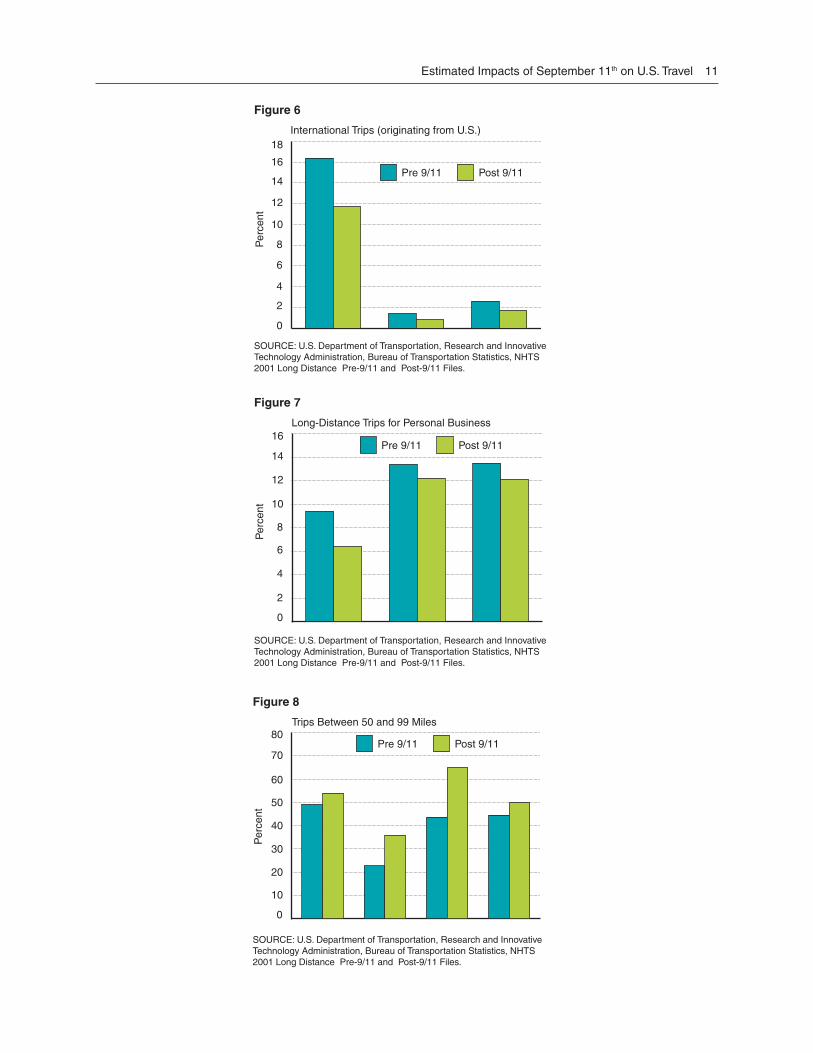
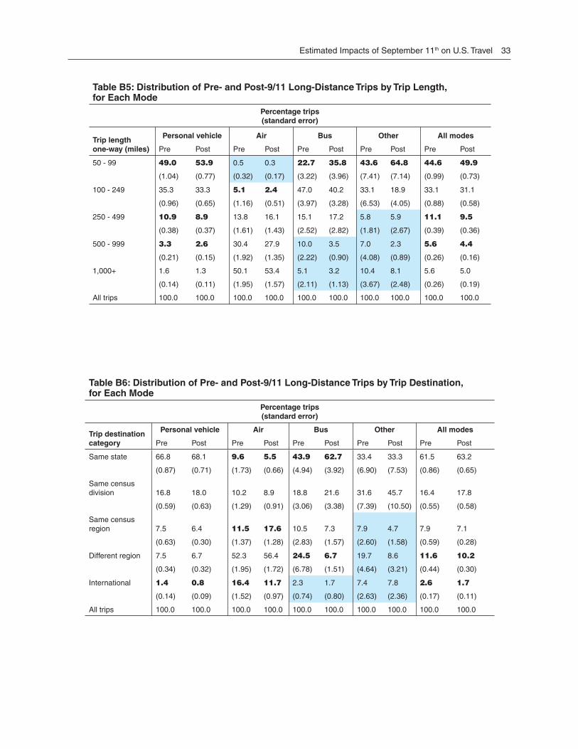
Prior to 9/11, international travel (originating from the United States) represented 3 per-cent of all long-distance trips, but after 9/11 that travel dropped to 2 percent of all trips, a statistically signifi cant decline. The mode with the largest decrease in international travel was air, which fell from 16 to 12 percent of all air trips after 9/11. Air travel accounts for ap-proximately one-half of all international trips. POV long-distance trips for international travel experienced a small decline after 9/11 (fi gure 6). POV travel accounts for slightly more than 40 percent of international trips.
Personal Business Travel Decreased
Long-distance trips for personal business also experienced a statistically signifi cant decline
after 9/11, from nearly 14 percent of all trips to 12 percent. Personal business trips include medical visits, shopping trips, and trips to attend weddings and funerals. POV accounts for approximately 90 percent of all long-distance personal business trips. Air travel, which accounts for only about 5 percent of all personal business trips, experienced a 3 percent decrease from 9 to 6 percent of air trips (fi gure 7).
More Shorter Distance Trips Taken
The only trip distance that showed a signifi -cant increase after 9/11 was in the shortest distance category of between 50 to 99 miles. All modes combined in this distance category showed an increase from 45 to 50 percent of total trips after 9/11 (fi gure 8). POV trips, which account for more than 95 percent of all trips between 50 to 99 miles, increased from 49 to 54 percent after 9/11, bus trips increased from 23 to 36 percent, and the “other” category increased from 44 to 65 per-cent. Air was the only mode not to register a signifi cant increase, but air travel accounts for a negligible portion (nearly zero percent) of the trips in the 50 to 99 mile range. Modes that were not statistically signifi cant were not included in the fi gures.
Appendix A describes the methodology of the NHTS and how the pre-9/11 and post-9/11 data fi les were created. Appendix B contains tables with the data estimates used in this report and their standard errors. Standard errors are in the same metric as the estimates. All comparisons in the text and graphics are statistically signifi cant at a 0.05 level unless otherwise noted.
Estimated Impacts of September 11th on U.S. Travel 11
Figure 6
0
2
4
6
8
10
12
14
16
18
Per
cent
Pre 9/11 Post 9/11
International Trips (originating from U.S.)
SOURCE: U.S. Department of Transportation, Research and Innovative Technology Administration, Bureau of Transportation Statistics, NHTS 2001 Long Distance Pre-9/11 and Post-9/11 Files.
Figure 7
0
2
4
6
8
10
12
14
16
Per
cent
Pre 9/11 Post 9/11
Long-Distance Trips for Personal Business
SOURCE: U.S. Department of Transportation, Research and Innovative Technology Administration, Bureau of Transportation Statistics, NHTS 2001 Long Distance Pre-9/11 and Post-9/11 Files.
Figure 8
0
10
20
30
40
50
60
70
80
Per
cent
Pre 9/11 Post 9/11
Trips Between 50 and 99 Miles
SOURCE: U.S. Department of Transportation, Research and Innovative Technology Administration, Bureau of Transportation Statistics, NHTS 2001 Long Distance Pre-9/11 and Post-9/11 Files.
12 Estimated Impacts of September 11th on U.S. Travel
Expected Results Not Observed
Immediately following the 9/11 terrorist attack, experts were trying to determine how these attacks would impact our economy, business and leisure travel, and the attitudes of Americans. The terrorist attack was ex-pected to have a different degree of impact on the various travel markets. Here are some of the expected repercussions that were not borne out by the NHTS data:
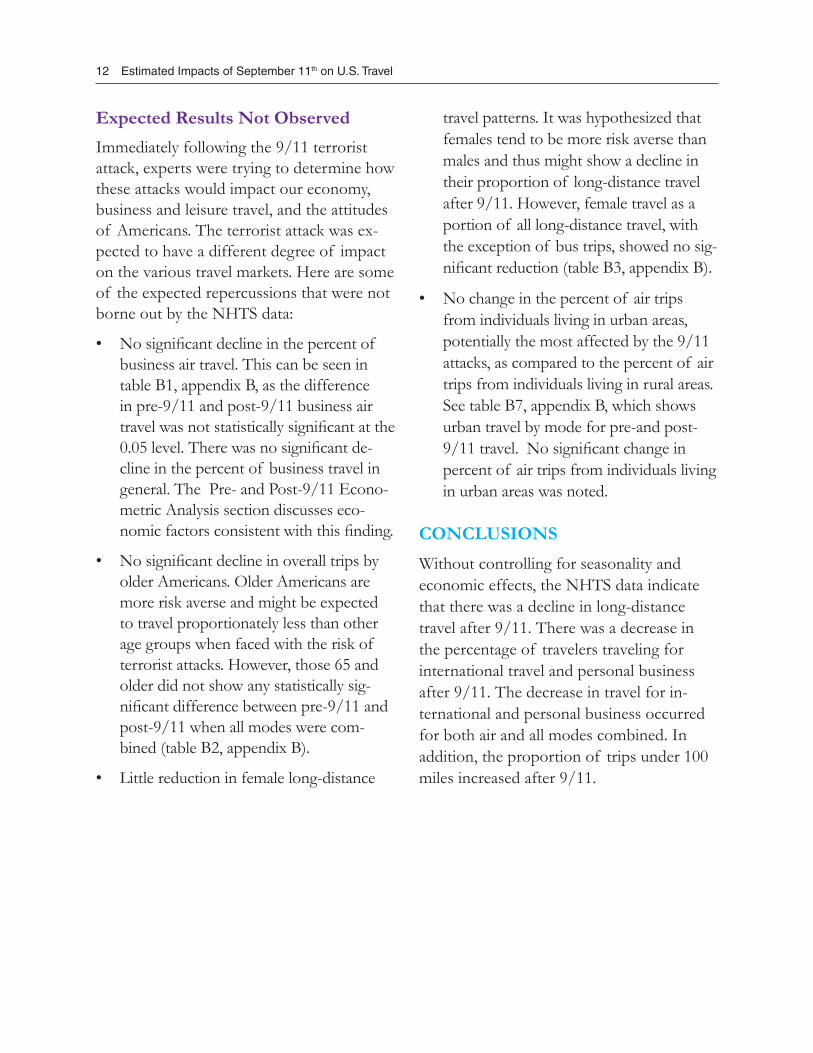
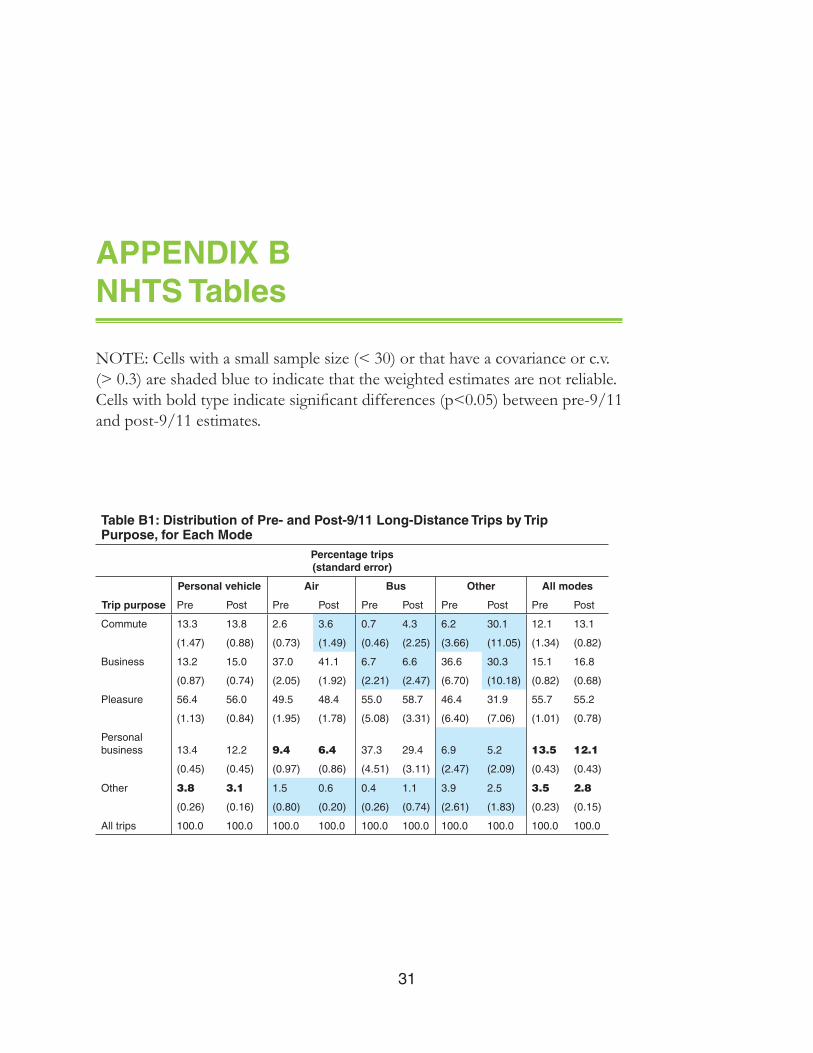
No signifi cant decline in the percent of business air travel. This can be seen in table B1, appendix B, as the difference in pre-9/11 and post-9/11 business air travel was not statistically signifi cant at the 0.05 level. There was no signifi cant de-cline in the percent of business travel in general. The Pre- and Post-9/11 Econo-metric Analysis section discusses eco-nomic factors consistent with this fi nding.
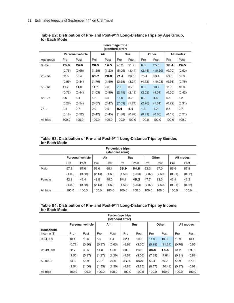
No signifi cant decline in overall trips by older Americans. Older Americans are more risk averse and might be expected to travel proportionately less than other age groups when faced with the risk of terrorist attacks. However, those 65 and older did not show any statistically sig-nifi cant difference between pre-9/11 and post-9/11 when all modes were com-bined (table B2, appendix B).
Little reduction in female long-distance
•
•
•
travel patterns. It was hypothesized that females tend to be more risk averse than males and thus might show a decline in their proportion of long-distance travel after 9/11. However, female travel as a portion of all long-distance travel, with the exception of bus trips, showed no sig-nifi cant reduction (table B3, appendix B).
No change in the percent of air trips from individuals living in urban areas, potentially the most affected by the 9/11 attacks, as compared to the percent of air trips from individuals living in rural areas. See table B7, appendix B, which shows urban travel by mode for pre-and post-9/11 travel. No signifi cant change in percent of air trips from individuals living in urban areas was noted.
CONCLUSIONS
Without controlling for seasonality and economic effects, the NHTS data indicate that there was a decline in long-distance travel after 9/11. There was a decrease in the percentage of travelers traveling for international travel and personal business after 9/11. The decrease in travel for in-ternational and personal business occurred for both air and all modes combined. In addition, the proportion of trips under 100 miles increased after 9/11.
•

13
CHAPTER 2Time Series Analysis of Passenger Data: Pre- and Post- September 11, 2001
INTRODUCTION
In the previous chapter, we noted that some of the differences between the pre- and post-September 2001 data could be attributed to the nature of time
series data. Differences due to seasonality confound the measurement of the September 2001 impact. In order to understand the time series characteristics of the passenger data, we turn our attention to different sets of data that mea-sure monthly passenger movement. The following sections will analyze three sets of monthly data: air revenue passenger miles, rail passenger miles, and vehicle miles traveled. The data do not separate local and long-distance travel.
To measure the effect of September 11, 2001, we will forecast these three series based on the data from January 1990 through August 2001. The forecasts are then compared to what actually occurred in the data. Air showed the greatest differences: the values of the aviation time series began to enter the prediction intervals in December 2003, indicating that the aviation miles only began to approach in 2004 the previously expected values. Rail miles did not appear to experience an immediate impact from September 11, 2001. Vehicle miles expe-rienced a one-month drop for September 2001, and an additional one-month drop was also experienced for September 2002.
The following sections provide the details behind these fi ndings.
ABOUT THE DATA
The fi rst three fi gures (fi gures 9, 10, and 11) provide graphs of the passenger time series data: air revenue passenger miles (RPM), rail passenger miles (PM),

14 Estimated Impacts of September 11th on U.S. Travel
Figure 9
Jan1990
Jan1992
Jan1994
Jan1996
Jan1998
Jan2000
Jan2002
Jan2004
0
10
20
30
40
50
60
70
80Air Revenue Passenger Miles (billions)
SOURCE: U.S. Department of Transportation, Research and Innovative Technology Administration, Bureau of Transportation Statistics, Offi ce of Airline Information, Air Carrier Traffi c Statistics (Monthly T-100).
Figure 10
Jan1990
Jan1992
Jan1994
Jan1996
Jan1998
Jan2000
Jan2002
Jan2004
0
100
200
300
400
500
600
700Rail Passenger Miles (millions)
SOURCE: FRA, Offi ce of Safety website, Table 1.02 Operational Data Tables, available at http://safetydata.fra.dot.gov/Offi ceofSafety/
Figure 11
Jan1992
Jan1994
Jan1996
Jan1998
Jan2000
Jan2002
Jan2004
Jan1990
0
50
100
150
200
250
300Vehicle Miles Traveled (billions)
SOURCE: USDOT / Federal Highway Administration, Traffi c Volume Trends report available at http://www.fhwa.dot.gov/policy/ohpi/travel/index.htm

Estimated Impacts of September 11th on U.S. Travel 15
and vehicle miles traveled (VMT). The air RPM are found in the T-1 dataset compiled for the T-100 database, taken from the U.S. Department of Transportation, Research and Innovative Technology Administration, Bureau of Transportation Statistics (BTS), Offi ce of Airline Information (OAI). The data for rail PM are compiled from the U.S. Department of Transportation, Federal Railroad Administration (FRA), Offi ce of Safety. VMT data are taken from the Traf-fi c Volume Trends reports from the Federal Highway Administration, Offi ce of High-way Policy Information.3 The datasets to be studied are all monthly, and each time series initiates at January 1990. The data values for the three series are through June 2004. Each of the three graphs contains a vertical line indicating September 2001. (Appendix C provides a table with all the data.)
SEASONAL ANALYSIS
A quick perusal of the three passenger data-sets reveals that the data are strongly season-al. But it is diffi cult to compare the degree of seasonality across the three time series. The next three graphs attempt to simplify the comparison. Figures 12, 13, and 14 pro-vide histograms of the seasonality of each series, which required an additional assump-tion that the seasonality of each series does not change much over time to justify averag-ing the monthly components. The seasonali-
3 Quality information on the air RPM and rail PM can be found at: http://www.bts.gov/programs/economics_and_fi nance/transportation_servic-es_index/html/source_and_documentation_and_data_quality.html. Information on the quality of the VMT data can be found at: http://www.fhwa.dot.gov/ohim/tvtw/tvtpage.htm.
ty is measured as the percent deviation from the underlying trend and consists of the average for the fi ve years of monthly data prior to September 2001, that is, September 1996 through August 2001. The method for decomposing the seasonality and the trend will be dealt with in the next section.
Note that the vertical axis for each graph runs from +25% to -25% deviation. In this way, the degree of deviation is comparable across the fi gures. While the patterns of sea-sonality are comparable (less travel in winter, and more travel in summer), we note that rail PM tends to vary the most and VMT the least. Part of this may be accounted for by the fact that rail deals with fewer miles, while VMT incorporates more; extreme val-ues have less of an impact when the number of observations is large.
The next section describes how the seasonal and trend components were created.
STAMP MODELING
One approach to studying seasonality is to decompose a time series into three compo-nents: the trend, the seasonal factors, and the irregular components. STAMP, which stands for Structural Time Series Analyser, Modeller and Predictor,4 allows us to take a set of time series data and break that dataset down (or “decompose” it) into components that cannot be observed directly, but have intuitive appeal. Most readers have an under-standing that a trend component will repre-sent the long-term direction of the data; a seasonal component will refl ect changes due
4 See Koopman et al. (2000) for more detail on STAMP.

16 Estimated Impacts of September 11th on U.S. Travel
Figure 12
Jan
Feb Mar Apr
May Ju
nJu
lAug Sep Oct
Nov Dec–25
–20
–15
–10
–5
0
5
10
15
20
25
Per
cent
dev
iatio
n fr
om tr
end
5 Year Average of Air Revenue Passenger Mile Seasonality
SOURCE: U.S. Department of Transportation, Research and Innova-tive Technology Administration, Bureau of Transportation Statistics.
Figure 13
Jan
Feb Mar Apr
May Ju
nJu
lAug Sep Oct
Nov Dec–25
–20
–15
–10
–5
0
5
10
15
20
25
Per
cent
dev
iatio
n fr
om tr
end
5 Year Average of Rail Passenger Mile Seasonality
SOURCE: U.S. Department of Transportation, Research and Innova-tive Technology Administration, Bureau of Transportation Statistics.
Figure 14
–25
–20
–15
–10
–5
0
5
10
15
20
25
Jan
Feb Mar Apr
May Ju
nJu
lAug Sep Oct
Nov Dec
Per
cent
dev
iatio
n fr
om tr
end
5 Year Average of Vehicle Miles Traveled Seasonality
SOURCE: U.S. Department of Transportation, Research and Innovative Technology Administration, Bureau of Transportation Statistics.

Estimated Impacts of September 11th on U.S. Travel 17
to the time within the year; and the irregular component will illustrate what is “left-over” or not explained by the trend or seasonal behavior. (For an explanation of the theory, the reader can obtain the details in appendix D.) These three components can be stochas-tic, or changing over time (S); fi xed, or un-changing over time (F); or nonexistent (N). Through statistical testing, we ascertained the best fi tting model for each time series for the time period of January 1990 through August 2001 (see table 1). By fi tting the data prior to September 2001, we can then forecast that model out through the current time and compare the results of these pre-September 2001 forecasts to the actual data.
Table 1: STAMP Model Specifi cations for Passenger Time Series.Passenger Mode Level S/F/N Slope S/F/N
Season S/F/N
Air RPM S F S
Rail PM S N S
VMT S F S
NOTE: S = stochastic, F =fi xed, N = nonexistent
While all three series have models with levels and seasonality changing stochastically over time, the air RPM and VMT exhibit fi xed un-derlying trends. The rail PM has no long-term trend for the period under study.
Using the above models, we forecast from September 2001 through December 2004 to help us understand the changes that occurred over that forecast period. We next provide the graphs of the three sets of data, with forecasts from September 2001 through December 2004 (fi gures 15, 16, and 17). The prediction intervals for the forecasts are also provided.
The following three graphs (fi gures 18, 19, and 20) provide a comparison of the forecasts
based on the pre-September 2001 data with the actual data from September 2001 forward. The large Is on the graphs indicate the values within the prediction interval.
As was expected, air RPM experienced the greatest impact. The forecasted RPMs and the actual RPMs have yet to match one another; only in 2004 did the actual air RPMs cross over into and remain in the 95 percent predic-tion interval, which indicates that aviation only began to return to what would have been the expected set of RPMs in 2004. Rail PM actu-als tended to be close to the forecasted values. VMT seems to show little difference between the actuals and the forecasts, with the excep-tion of the months of September 2001 and September 2002, thereby indicating little long-term impact on overall VMT levels.
In order to more accurately defi ne the im-pact of September 2001 on the actual data, we attempted to model the impact of Sep-tember 11, 2001, using the full set of data (January 1990 to June 2004), with the three-step intervention procedure developed by Ord and Young (2004). Three components of the intervention are tested: an additive outlier (AO) on September 2001, a tempo-rary decay (TC) starting October 2001, and a level shift (LS) starting November 2001.
For air RPM, the AO was signifi cant, as was expected; the TC of 8 percent 5 also proved to be signifi cant. The LS term was not sig-nifi cant – indicating that there may not be a permanent shift downward in the trend of the time series.
5 Four decay rates were tested: 6, 7, 8, and 9 percent. For air RPM, the best fi tting decay rate was 8 per-cent, which results in a half-life of 3 months beyond September, or December 2001.

18 Estimated Impacts of September 11th on U.S. Travel
Figure 15
Oct1995
Oct1996
Oct1997
Oct1998
Oct1999
Oct2000
Oct2001
Oct2002
Oct2003
Oct2004
40
50
60
70
80Forecasts of Air Revenue Passenger Miles (billions)
Air RPM
Lower prediction interval
Upper prediction interval
SOURCE: U.S. Department of Transportation, Research and Innova-tive Technology Administration, Bureau of Transportation Statistics.
Figure 16
Oct1995
Oct1996
Oct1997
Oct1998
Oct1999
Oct2000
Oct2001
Oct2002
Oct2003
Oct2004
300
350
400
450
500
550
600
650
700
Rail PM
Lower prediction interval
Upper prediction interval
Forecasts of Railroad Passenger Miles (millions)
SOURCE: U.S. Department of Transportation, Research and Innova-tive Technology Administration, Bureau of Transportation Statistics.
Figure 17
150
170
190
210
230
250
270
290
Oct1995
Oct1996
Oct1997
Oct1998
Oct1999
Oct2000
Oct2001
Oct2002
Oct2003
Oct2004
Forecasts of Vehicle Miles Traveled (billions)
VMT
Lower prediction interval
Upper prediction interval
SOURCE: U.S. Department of Transportation, Research and Innova-tive Technology Administration, Bureau of Transportation Statistics.

Estimated Impacts of September 11th on U.S. Travel 19
Figure 18
Jan2001
Jul2001
Jan2002
Jul2002
Jan2003
Jul2003
Jan2004
Jul2004
30
40
50
60
70
80Air Revenue Passenger Miles (billions)
Forecast of Air RPM before 9-11
Air RPM
SOURCE: U.S. Department of Transportation, Research and Innovative Technology Administration, Bureau of Transportation Statistics.
Figure 19
Jan2001
Jul2001
Jan2002
Jul2002
Jan2003
Jul2003
Jan2004
Jul2004
300
400
500
600
700Rail Passenger Miles (millions)
Forecasts of Rail PM
Rail PM
SOURCE: U.S. Department of Transportation, Research and Innovative Technology Administration, Bureau of Transportation Statistics.
Figure 20
Jan2001
Jul2001
Jan2002
Jul2002
Jan2003
Jul2003
Jan2004
Jul2004
200
220
240
260
280Vehicle Miles Traveled (billions)
Forecast of VMT
VMT
SOURCE: U.S. Department of Transportation, Research and Innovative Technology Administration, Bureau of Transportation Statistics.

20 Estimated Impacts of September 11th on U.S. Travel
For rail RPM, none of the three-step inter-vention terms were signifi cant, indicating that September 2001 did not have a signifi cant impact on the series. However, as can be seen in the graph, there was an unexpected short-term drop in the rail PM the following year (September through November), which may indicate an avoidance of travel on the one-year anniversary.
For VMT, the AO at September 2001 was signifi cant, but then the data returned to the expected pattern. So it may be that people avoided car travel in September 2001, but then returned to their usual driving behavior the following month. The summary of these intervention results are provided in table 2.
The next section conducts an analysis com-paring the NHTS data with the time series analysis; the time series summaries used in the analysis are available in appendix E.
COMPARISON OF PRE- AND POST- 9/11 MONTHLY TRIPS
In order to simplify the comparison between the time series analysis and the NHTS data, only the forecast results from the time series analysis for the months of the NHTS data collection are considered. The three tables in appendix E show, according to the time series forecasting, both the actual values and the forecasts, along with the corresponding calculated forecast errors.
The travel estimates by mode presented in appendix E can be compared to the NHTS trip estimates to indicate what portion, if any, of the changes in the number of trips between the NHTS pre-and post-9/11 data-sets can be attributed to the events of 9/11
and the following months covered by the NHTS survey.
Both the pre-and post-9/11 NHTS datasets were reweighted to give annual trip estimates for the U.S. population. However, the sur-vey periods covered by each dataset do not give equivalent time periods before and after September 11, 2001. The NHTS survey was conducted from March 2001 to May 2002. The pre-and post-9/11 datasets divide the persons surveyed during that period into two groups, March 2001 to September 11, 2001 in the pre-9/11 dataset, and Septem-ber 12, 2001 to May 2002 in the post-9/11 dataset. The pre-9/11 dataset covers three full months and parts of four other months. The post-9/11 dataset covers 5 full months and parts of 4 other months. The repeated months between the two datasets include March 2001 and March 2002, April 2001 and April 2002, May 2001 and May 2002, and the pre-and post-9/11 portions of September 2001. As a consequence of the unequal time periods covered in each datas-et, the total number of estimated trips from each dataset cannot be compared to each other. However, it is possible to compare the trip estimates by calculating a monthly average number of trips from each dataset to adjust for the unequal time periods. Table 3 gives the comparison of NHTS monthly trip estimates to the travel estimates by mode in tables E1 through E3.
Unfortunately the comparisons are very rough. For highways, vehicle miles traveled includes all personal vehicle, public transit, and freight travel over all public highways in the United States. This is compared to NHTS trip estimates that include only long-

Estimated Impacts of September 11th on U.S. Travel 21
Table 2: Intervention Analysis in STAMP on Passenger Time Series.
Passenger modeAdditive Outlier (AO)
Sep-01Temporary Change (TC)
Oct-01Level Shift (LS)
Nov-01
Air RPM Signifi cant Signifi cant (decay rate = 8%) Not Signifi cant
Rail PM Not Signifi cant Not Signifi cant Not Signifi cant
VMT Signifi cant Not Signifi cant Not Signifi cant
SOURCE: STAMP analysis, U.S. Department of Transportation, Research and Innovative Technology Administration, Bureau of Transportation Statistics.
Table 3: Comparison of NHTS Trip Estimates to Other Travel DataMonthly averagepre-9/11 period
(Mar. 2001-Sept. 11 2001)
Monthly averagepost-9/11 period
(Sept. 12, 2001 - May 2002) Percent change
Vehicle Miles Traveled
Actual 242.3 225.1 -7.1
Forecast in absence of 9/11 242.3 225 -7.2
NHTS Personal Vehicle Trips (millions)
Estimated 201.8 181.2 -10.2
Air RPM (millions.)
Actual 63.1 46.4 -26.4
Forecast in absence of 9/11 63.1 58.1 -7.8
NHTS Air Trips (millions)
Estimated 18.0 14.1 -21.7
Rail RPM (millions.)
Actual 508.3 439.1 -13.6
Forecast in absence of 9/11 508.3 436.4 -14.1
NHTS Train Trips (millions.)
Estimated 1.7 1.6 -5.5
NHTS Bus Trips (millions.)
Estimated 5.1 4.5 -12.1
SOURCE: U.S. Department of Transportation, Research and Innovative Technology Administration, Bureau of Transportation Statistics.
NOTE: Shaded difference not signifi cant at a 0.05 level. Pre- and Post-9/11 monthly estimates of VMT are prorated for the NHTS survey overlap months of March, April, and May 2001 and 2002, using NHTS pre-and post-9/11 datasets. The weights for the overlap months are calculated using the proportion of trips taken in those months from the pre-and post-9/11 datasets. September 2001 is prorated using 0.33 for the pre-9/11 weight, and 0.67 for the post-9/11 weight.

22 Estimated Impacts of September 11th on U.S. Travel
distance personal vehicle trips. For passen-ger rail, Amtrak passenger data is compared to the NHTS long-distance trips by rail, which likely includes some commuter rail trips. There are no long-distance bus data available for comparison to the NHTS bus trip estimates.
Air trips provide the most interesting com-parison. Average monthly air RPM experi-enced a drop of 26.4 percent between the pre-9/11 time period and the post-9/11 time period. When the post-9/11 time period was forecast using previous historical trends, the drop was only 7.8 percent. The difference
between those two percentage decreases, about 18.6 percent, can be viewed as the ad-ditional decrease in air travel beyond normal historical seasonal trends. The estimated decline from NHTS data of about 22 per-cent is roughly comparable to the 26 percent decline in air RPM. While the 22 percent cannot be divided up into seasonal and non-seasonal components, using the proportion-al change in air RPM as a proxy, this gives roughly about a 6 to 7 percent decline for normal seasonal trends and the rest, about 15 to 16 percent, can be attributed to other factors, including 9/11.

23
CHAPTER 3Pre- and Post-9/11 Econometric Analysis of Travel by Mode
PREFACE
The following analysis supplements the previous chapters, which initially reviewed the NHTS datasets and then developed seasonally adjusted time
series travel estimates. The econometric analysis to follow includes equation estimates for three modes of travel: air, highway, and rail passenger. Each equation will be reviewed for statistical qualities, followed by a discussion that will establish a relationship between travel by mode and the catastrophic events of 9/11.
DATA The seasonally adjusted monthly travel data used in the econometric analysis spans the period of January 2000 through June 2003, and is identical to the data used in the time series analysis. The exponential weights for the dummy vari-able used in the VMT equation for the 5-month period from September 2001 to January 2002 are: 1.000, 0.6494, 0.4217, 0.2738, and 0.1778. These weights were approximated by applying a standard natural exponential curve to the data, which would result in a function ranging from 1.0 to 0. These 5 months were chosen based on their proximity to 9/11 and appeared to be the time frame when travel appeared to be most affected by 9/11. Other time periods were chosen and were not found to be statistically signifi cant.
The economic data comes from the Economic Report of the President, which was obtained from the web.6 The fuel price data originates from the U.S. De-partment of Energy, Energy Information Administration. Revenue Passenger Miles per Departure data came from the Bureau of Transportation Statistics,
6 http://www.gpoaccess.gov/eop/

24 Estimated Impacts of September 11th on U.S. Travel
Offi ce of Airline Information. Although the equations listed in the tables below contain only those variables that were statistically signifi cant, several variables were tested, but did not meet the statistical signifi cance tests at either the 5 or 10 percent probability levels. The variables that were excluded in the equations consisted of industrial produc-tion and wholesale and retail sales. However, all variables were tried in logarithmic and lagged conversions, and equation specifi ca-tions were estimated in linear and nonlinear formats.
METHODOLOGY
Travel was econometrically estimated for aviation, highway, and rail passenger modes from monthly data. Both linear and log specifi cations were tested with combinations of the following economic variables: unem-ployment, wholesale and retail sales, indus-trial production, income per driver, fuel prices by mode and fuel type or fuel cost per mile. Two types of dummy variables were used, a typical 0,1 value for September 2001 through February 2002, and another with an exponential decay curve. Corrective procedures were also implemented when needed, such as those associated with serial or time dependent correlation over several periods. Lagged vari-ables through two time periods were also used, and in cases where serial correlation were present, AR(1) (auto-regressive terms of one period) were then included in the estimations. Other
independent variables were also used, such as the airline revenue passenger miles per departure. In all, over 30 estimations per mode were attempted with varying combi-nations of variables and equation specifi ca-tions.
RESULTS AND STATISTICAL ANALYSIS
Aviation
The results of the aviation estimation (table 4) indicate that there was a statistically sig-nifi cant negative impact of 9/11 on air trav-el per person above age 16. Other relevant variables such as income per person above age 16, jet fuel price, and the unemployment rate were signifi cant as well, with all vari-ables statistically signifi cant at the α = 0.01 level. All variables have the correct a priori mathematical sign. For example, income has a positive effect on travel, while both unem-ployment and jet fuel price negatively impact travel.
Overall, the statistical fi t accounts for 51 percent of the variation from the dependent
Table 4: Seasonally Adjusted Aviation Revenue Passenger-Miles per Driving Age 16+ Population Equation Estimation with Unemploy-ment VariableDependent Variable: Aviation Revenue Passenger Miles (seasonally adjusted) per Population Driving Age 16+
Method: Least Squares
Sample: January 2000 to June 2003
Included observations: 42
Variable Coeffi cient Standard error t-statistic Probability
Income per population age 16+ 0.014 0.002 9.171 0.000
Jet fuel price -0.195 0.064 -3.018 0.005
Dummy 9/11 -105.270 20.604 -5.109 0.000
Unemployment -26.308 8.148 -3.229 0.003
R-squared 0.512
Adjusted R-squared 0.474SOURCE: U.S. Department of Transportation, Research and Innovative Technology Administration, Bureau of Transportation Statistics.
Estimated Impacts of September 11th on U.S. Travel 25
variable mean. The Durbin-Watson test is inconclusive for autocorrelation among er-ror terms, so no adjustments were made to the original equation.
Where:
Income per population aged 16+ = income7 per population aged 16+8 (in real 1996 dol-lars per population aged 16 and over)
Jet fuel price = kero-jet fuel price9 (1/10th
cent per bbl in nominal dollars)
Dummy 9/11 = dummy variable, where value equals 1 for September 2001 through February 2002
Unemployment = unemployment (percent)10
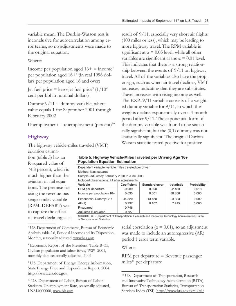
Highway
The highway vehicle-miles traveled (VMT) equation estima-tion (table 5) has an R-squared value of 74.8 percent, which is much higher than the aviation or rail equa-tions. The premise for using the revenue-pas-senger miles variable (RPM_DEPART) was to capture the effect of travel declining as a
7 U.S. Department of Commerce, Bureau of Economic Analysis, table 2.6, Personal Income and Its Disposition, Monthly, seasonally adjusted, www.bea.gov.8 Economic Report of the President, Table B–35, Civilian population and labor force, 1929–2001, monthly data seasonally adjusted, 2004.9 U.S. Department of Energy, Energy Information, State Energy Price and Expenditure Report, 2004. http://www.eia.doe.gov.10 U.S. Department of Labor, Bureau of Labor Statistics, Unemployment Rate, seasonally adjusted, LNS14000000, www.bls.gov.
result of 9/11, especially very short air fl ights (100 miles or less), which may be leading to more highway travel. The RPM variable is signifi cant at α = 0.05 level, while all other variables are signifi cant at the α = 0.01 level. This indicates that there is a strong relation-ship between the events of 9/11 on highway travel. All of the variables also have the prop-er sign, such as when air travel declines, VMT increases, indicating that they are substitutes. Travel increases with rising income as well. The EXP_9/11 variable consists of a weight-ed dummy variable for 9/11, in which the weights decline exponentially over a 4-month period after 9/11. The exponential form of the dummy variable was found to be statisti-cally signifi cant, but the (0,1) dummy was not statistically signifi cant. The original Durbin-Watson statistic tested positive for positive
serial correlation (α = 0.01), so an adjustment was made to include an autoregressive (AR) period 1 error term variable.
Where:
RPM per departure = Revenue passenger miles11 per departure
11 U.S. Department of Transportation, Research and Innovative Technology Administration (RITA), Bureau of Transportation Statistics, Transportation Services Index (TSI), http://www.bts.gov/xml/tsi/
Table 5: Highway Vehicle-Miles Traveled per Driving Age 16+ Population Equation EstimationDependent variable: vehicle miles traveled per driverMethod: least squaresSample (adjusted): February 2000 to June 2003Included observations: 41 after adjustmentsVariable Coeffi cient Standard error t-statistic Probability RPM per departure -0.989 0.398 -2.483 0.018Income per population 16+ 0.035 0.001 58.356 0.000
Exponential Dummy 9/11 -44.820 13.488 -3.323 0.002AR(1) 0.797 0.107 7.415 0.000R-squared 0.748 Adjusted R-squared 0.727 SOURCE: U.S. Department of Transportation, Research and Innovative Technology Administration, Bureau of Transportation Statistics.

26 Estimated Impacts of September 11th on U.S. Travel
Exponential Dummy 9/11 = exponentially weighted dummy variable, where value ex-ponentially decays through 4 time periods.
AR(1) = Auto-regressive error terms of time period one12
Rail
Only the logarithmic equation specifi ca-tion (table 6) was found to be statistically acceptable, in terms of fi t and statistical signifi cance. Notice that the equation has no 9/11 variable, because it was found to not be statistically signifi cant in all combinations of log and linear specifi cations as well as combinations of all variables. Both the log
of the time period lag of one for the depen-dent variable and the log of the income per driver were found to be statistically signifi -cant. Each variable has the proper positive sign indicating that rail passenger travel rises as a result of the effects of the previ-ous time period and the effects of increases
src/index.xml and National Transportation Statistics, http://www.bts.gov/publiications/national_transpor-tation_statistics//2005/index.html, 2005.12 See William Greene, Econometric Analysis, 2003.
in income per driver. The Durbin-Watson statistic revealed no serial correlation.
DISCUSSION
Economic Demand Elasticities Com-parison
Often an evaluation of econometric equa-tions includes comparisons to other esti-mates using the estimated coeffi cients to develop economic elasticities. Demand elasticities measure the degree, in percent-age change, to which one economic variable changes based on the percentage change of another economic variable. Table 7 shows
a comparison be-tween demand elas-ticities from the BTS study versus Carol Dahl’s compilation of various model elasticities.13 All of the BTS elasticities were calculated at the mean and are very close or within the range of Carol Dahl’s fi ndings, possibly
with the exception of the aviation income elasticity, which appears to be larger than the
13 Carol Dahl, Professor, Director of CSM/IFP Joint International Degree Program in Petroleum Economics and Management, Colorado School of Mines, Golden, Colorado. Dahl has compiled de-mand equation elasticities for 20 authors, many with multiple estimations over time. They are categorized according to equation specifi cations and type of data used. Elasticities are derived from equation coeffi cients in the form of a percentage change in demand for a percentage change in price or income.
Table 6: Log of Seasonally Adjusted Passenger-Miles for Rail per Driving Age 16+ Population Equation EstimationDependent variable: Log Rail Passenger-miles per Population Aged 16+ (seasonally adjusted)
Method: Least Squares
Sample (adjusted): February 2000 to June 2003
Included observations: 41 after adjustments
Variable Coeffi cient Standard error t-statistic Probability
Log of seasonally adjusted rail passenger miles per population aged 16+ lagged one period 0.767 0.105 7.301 0.000
Log of income per population aged 16+ 0.175 0.079 2.223 0.032
R-squared 0.537
Adjusted R-squared 0.525 SOURCE: U.S. Department of Transportation, Research and Innovative Technology Administration, Bureau of Transportation Statistics.

Estimated Impacts of September 11th on U.S. Travel 27
higher range of the estimates (Dahl, 1995). It should also be noted that Dahl’s elasticities are measured with respect to transportation fuel consumption and are not as specifi c to a particular mode as the BTS study. Therefore,
the elasticities should be judged in a more general manner than viewed as exact com-parisons by mode.
The results indicate that there is a strong statistical relationship between the events of 9/11 and aviation and highway travel, but not rail revenue passenger miles. Given that the 9/11 dummy variables are statisti-cally signifi cant, it can be concluded that the negative effect of 9/11 on travel declines in a more arithmetic fashion for air travel over a 6 month period, in which there is a decline
in the intercept. Similarly, highway travel has a tendency to decline in a more exponential pattern over a 4-month period. These con-clusions do not attempt to determine when travel will return to a more normal historical level, but rather only the declining portion of the travel. Furthermore, it can be con-cluded that there is a statistically signifi cant substitution relationship between air travel and highway travel, although the cross elas-ticity is small at -0.041. This cross elasticity was derived from the air travel coeffi cient and indicates that for each 100 percent drop in air travel, highway travel will increase at approximately 4.1 percent.
The conclusions of this study do not equate to assuming that future catastrophic events would yield the same results because the degree of damage and the impending effect on behavior may not be the same for future events. The severity of catastrophic events and their impact on future behavior is not easily quantifi able, and yet is essential for future analysis of catastrophic events. Hope-fully future research and analysis will lead to some kind of indicator of the degree of severity of catastrophes.
Table 7: Economic Demand Elasticities Aviation Highway Rail Dahl
Income elasticity 1.74 1.04 0.18 0.09 to 0.85
Fuel price elasticity -0.38 - - -0.01 to -0.36
SOURCE: Dahl, Carol A. “Demand for Transportation Fuels: A Sur-vey of Demand Elasticities and Their Components,” Journal of Energy Literature, 1(2), Fall, 1995. and U.S. Department of Transportation, Research and Innovative Technology Administration, Bureau of Transportation Statistics.


29
APPENDIX AMethodology
SOURCE AND ACCURACY
The fi ndings from the 2001 NHTS survey are based on travel data collected from a random digit dial sample of telephone interviews conducted with over 60,000 individuals in approximately 26,000 nationally representative households. Interviews were conducted between March 2001 and May 2002. Individuals in the NHTS sample were asked to complete a travel diary for a specifi ed day, known as the travel day, and were also asked to report on the characteristics of long-distance trips of 50 miles or more from home made during a 4-week period, known as the travel period.
Estimates reported here are based on weighted data to account for selection probabilities at the household and individual level, and are further adjusted for household and individual nonresponse. Comparisons made in this report are statistically signifi cant at a 0.05 level.
CREATION OF PRE-9/11 AND POST-9/11 DATA FILES
The 2001 NHTS was conducted from March 2001 through May 2002. The NHTS person-level dataset was divided into two parts: pre-9/11 data and post-9/11 data. The pre-9/11 dataset includes trips taken in the period from March 2001 to September 2001, a period of 5 1/2 months, and includes the summer season in which a large proportion of long-distance trips are taken. There were approximately 22,000 persons responding about travel prior to 9/11. The post-9/11 dataset includes trips taken in the period from Septem-ber 2001 to May 2002, a period of roughly 8 months, and includes Thanksgiv-ing and Christmas—a traditionally heavy season for long-distance trips. The survey had responses from approximately 38,000 persons on their long-dis-tance trips after 9/11. The composition of persons who took long-distance trips prior to 9/11 and those that took long-distance trips following 9/11 was not the same. A more detailed description of how the pre-9/11 and post-

30 Estimated Impacts of September 11th on U.S. Travel
9/11 data fi les were created is contained in Chapter 1 of “National Household Travel Survey—Pre- and Post-Data Documenta-tion” found on www.bts.gov.
Additional steps were taken to make each of the pre-9/11 and post-9/11 groups a nationally representative sample. This is achieved by constructing new weights using statistically sound methods briefl y described below.
REWEIGHTING OF PRE-9/11 AND POST-9/11 DATA FILES
Weights are needed to produce valid popula-tion-level estimates so that the results of a survey of the population are representative of the population as a whole. For example, if in the survey 47 percent of the respon-dents were male and in the U.S. population 49 percent of the population was known to be male, then the male survey respondents would be weighted stronger so that their data and travel information would count for 49 percent of the population’s travel pat-
terns. Adjustment and post-stratifi cation are performed on collected data to reduce bias of estimates. Post-stratifi cation reweights the data so that the characteristics of the re-spondents are the same as the characteristics of the population.
To see whether the pre- and post- 9/11 groups were representative samples of the national population it was necessary to construct population control totals for key survey variables using Census 2000 num-bers. Tolerance levels were used in the fi nal reweighting program to determine which combination of variables to keep. An ex-ample of a tolerance level would be for His-panics to be within 4 persons of a census generated control total that would represent the total Hispanics in the United States for a designated timeframe. A more detailed description of how the pre-9/11 and post-9/11 data fi les were reweighted is contained in chapter 2 of “National Household Travel Survey- Pre- and Post-Data Documenta-tion” found on www.bts.gov.
31
APPENDIX B NHTS Tables
NOTE: Cells with a small sample size (< 30) or that have a covariance or c.v. (> 0.3) are shaded blue to indicate that the weighted estimates are not reliable. Cells with bold type indicate signifi cant differences (p<0.05) between pre-9/11 and post-9/11 estimates.
Table B1: Distribution of Pre- and Post-9/11 Long-Distance Trips by Trip Purpose, for Each Mode
Percentage trips(standard error)
Trip purpose
Personal vehicle Air Bus Other All modes
Pre Post Pre Post Pre Post Pre Post Pre Post
Commute 13.3 13.8 2.6 3.6 0.7 4.3 6.2 30.1 12.1 13.1
(1.47) (0.88) (0.73) (1.49) (0.46) (2.25) (3.66) (11.05) (1.34) (0.82)
Business 13.2 15.0 37.0 41.1 6.7 6.6 36.6 30.3 15.1 16.8
(0.87) (0.74) (2.05) (1.92) (2.21) (2.47) (6.70) (10.18) (0.82) (0.68)
Pleasure 56.4 56.0 49.5 48.4 55.0 58.7 46.4 31.9 55.7 55.2
(1.13) (0.84) (1.95) (1.78) (5.08) (3.31) (6.40) (7.06) (1.01) (0.78)
Personal business 13.4 12.2 9.4 6.4 37.3 29.4 6.9 5.2 13.5 12.1
(0.45) (0.45) (0.97) (0.86) (4.51) (3.11) (2.47) (2.09) (0.43) (0.43)
Other 3.8 3.1 1.5 0.6 0.4 1.1 3.9 2.5 3.5 2.8
(0.26) (0.16) (0.80) (0.20) (0.26) (0.74) (2.61) (1.83) (0.23) (0.15)
All trips 100.0 100.0 100.0 100.0 100.0 100.0 100.0 100.0 100.0 100.0
32 Estimated Impacts of September 11th on U.S. Travel
Table B2: Distribution of Pre- and Post-9/11 Long-Distance Trips by Age Group, for Each Mode
Percentage trips(standard error)
Age group
Personal vehicle Air Bus Other All modes
Pre Post Pre Post Pre Post Pre Post Pre Post
0 - 24 26.6 24.6 20.5 14.5 46.2 51.9 6.8 25.0 26.4 24.5
(0.75) (0.68) (1.38) (1.23) (5.05) (3.44) (2.44) (10.50) (0.70) (0.63)
25 - 54 53.6 55.4 61.7 70.0 21.4 26.8 75.4 58.4 53.8 55.8
(0.99) (0.84) (1.70) (1.50) (3.68) (3.34) (4.72) (10.03) (0.91) (0.76)
55 - 64 11.7 11.0 11.7 9.6 7.0 8.7 8.0 10.7 11.6 10.8
(0.72) (0.44) (1.03) (0.80) (2.45) (2.19) (2.52) (4.51) (0.65) (0.42)
65 - 74 5.6 6.4 4.2 3.5 16.0 8.2 8.0 4.6 5.8 6.2
(0.26) (0.34) (0.87) (0.47) (7.03) (1.74) (2.76) (1.61) (0.29) (0.31)
75 + 2.4 2.7 2.0 2.5 9.4 4.5 1.8 1.2 2.5 2.7
(0.18) (0.22) (0.42) (0.45) (1.88) (0.97) (0.91) (0.66) (0.17) (0.21)
All trips 100.0 100.0 100.0 100.0 100.0 100.0 100.0 100.0 100.0 100.0
Table B3: Distribution of Pre- and Post-9/11 Long-Distance Trips by Gender, for Each Mode
Percentage trips(standard error)
Personal vehicle Air Bus Other All modes
Pre Post Pre Post Pre Post Pre Post Pre Post
Male 57.2 57.6 56.6 60.1 35.9 54.8 52.3 67.0 56.6 57.8
(1.00) (0.88) (2.14) (1.60) (4.50) (3.63) (7.87) (7.50) (0.91) (0.82)
Female 42.8 42.4 43.5 40.0 64.1 45.2 47.7 33.0 43.4 42.2
(1.00) (0.88) (2.14) (1.60) (4.50) (3.63) (7.87) (7.50) (0.91) (0.82)
All trips 100.0 100.0 100.0 100.0 100.0 100.0 100.0 100.0 100.0 100.0
Table B4: Distribution of Pre- and Post-9/11 Long-Distance Trips by Income, for Each Mode
Percentage trips(standard error)
Personal vehicle Air Bus Other All modes
Household income ($) Pre Post Pre Post Pre Post Pre Post Pre Post
0-24,999 13.1 13.6 5.9 4.4 32.1 18.5 11.0 19.3 12.9 13.1
(0.79) (0.60) (0.87) (0.63) (6.92) (3.00) (5.18) (11.24) (0.76) (0.55)
25-49,999 32.7 30.5 14.3 15.8 30.3 28.6 35.6 15.5 31.2 29.3
(1.00) (0.87) (1.27) (1.29) (4.51) (3.06) (7.59) (4.61) (0.91) (0.82)
50,000+ 54.3 55.9 79.7 79.8 37.6 52.9 53.4 65.2 55.9 57.6
(1.04) (1.00) (1.55) (1.39) (4.88) (3.85) (8.57) (10.49) (0.97) (0.92)
All trips 100.0 100.0 100.0 100.0 100.0 100.0 100.0 100.0 100.0 100.0
Estimated Impacts of September 11th on U.S. Travel 33
Table B5: Distribution of Pre- and Post-9/11 Long-Distance Trips by Trip Length, for Each Mode
Percentage trips(standard error)
Trip lengthone-way (miles)
Personal vehicle Air Bus Other All modes
Pre Post Pre Post Pre Post Pre Post Pre Post
50 - 99 49.0 53.9 0.5 0.3 22.7 35.8 43.6 64.8 44.6 49.9
(1.04) (0.77) (0.32) (0.17) (3.22) (3.96) (7.41) (7.14) (0.99) (0.73)
100 - 249 35.3 33.3 5.1 2.4 47.0 40.2 33.1 18.9 33.1 31.1
(0.96) (0.65) (1.16) (0.51) (3.97) (3.28) (6.53) (4.05) (0.88) (0.58)
250 - 499 10.9 8.9 13.8 16.1 15.1 17.2 5.8 5.9 11.1 9.5
(0.38) (0.37) (1.61) (1.43) (2.52) (2.82) (1.81) (2.67) (0.39) (0.36)
500 - 999 3.3 2.6 30.4 27.9 10.0 3.5 7.0 2.3 5.6 4.4
(0.21) (0.15) (1.92) (1.35) (2.22) (0.90) (4.08) (0.89) (0.26) (0.16)
1,000+ 1.6 1.3 50.1 53.4 5.1 3.2 10.4 8.1 5.6 5.0
(0.14) (0.11) (1.95) (1.57) (2.11) (1.13) (3.67) (2.48) (0.26) (0.19)
All trips 100.0 100.0 100.0 100.0 100.0 100.0 100.0 100.0 100.0 100.0
Table B6: Distribution of Pre- and Post-9/11 Long-Distance Trips by Trip Destination, for Each Mode
Percentage trips(standard error)
Trip destination category
Personal vehicle Air Bus Other All modes
Pre Post Pre Post Pre Post Pre Post Pre Post
Same state 66.8 68.1 9.6 5.5 43.9 62.7 33.4 33.3 61.5 63.2
(0.87) (0.71) (1.73) (0.66) (4.94) (3.92) (6.90) (7.53) (0.86) (0.65)
Same census division 16.8 18.0 10.2 8.9 18.8 21.6 31.6 45.7 16.4 17.8
(0.59) (0.63) (1.29) (0.91) (3.06) (3.38) (7.39) (10.50) (0.55) (0.58)
Same census region 7.5 6.4 11.5 17.6 10.5 7.3 7.9 4.7 7.9 7.1
(0.63) (0.30) (1.37) (1.28) (2.83) (1.57) (2.60) (1.58) (0.59) (0.28)
Different region 7.5 6.7 52.3 56.4 24.5 6.7 19.7 8.6 11.6 10.2
(0.34) (0.32) (1.95) (1.72) (6.78) (1.51) (4.64) (3.21) (0.44) (0.30)
International 1.4 0.8 16.4 11.7 2.3 1.7 7.4 7.8 2.6 1.7
(0.14) (0.09) (1.52) (0.97) (0.74) (0.80) (2.63) (2.36) (0.17) (0.11)
All trips 100.0 100.0 100.0 100.0 100.0 100.0 100.0 100.0 100.0 100.0

34 Estimated Impacts of September 11th on U.S. Travel
Table B7: Distribution of Pre- and Post-9/11 Long-Distance Trips by Area Type, for Each Mode
Percentage trips(standard error)
Area type
Personal vehicle Air Bus Other All modes
Pre Post Pre Post Pre Post Pre Post Pre Post
Urban 72.0 69.8 89.7 90.5 83.5 72.4 91.8 73.9 73.9 71.3
(1.08) (0.97) (1.03) (0.81) (2.80) (3.01) (4.54) (8.45) (0.97) (0.88)
Rural 28.0 30.2 10.3 9.5 16.5 27.6 8.2 26.1 26.2 28.7
(1.08) (0.97) (1.03) (0.81) (2.80) (3.01) (4.54) (8.45) (0.97) (0.88)
All trips 100.0 100.0 100.0 100.0 100.0 100.0 100.0 100.0 100.0 100.0
Table B8: Distribution of Pre- and Post-9/11 Long-Distance Trips by Mode, for Each Trip Purpose
Percentage trips(standard error)
Trip purpose
Personal vehicle Air Bus Other All modes
Pre Post Pre Post Pre Post Pre Post Pre Post
Commute 97.7 94.7 1.7 1.9 0.1 0.7 0.5 2.6 100.0 100.0
(0.56) (1.37) (0.52) (0.81) (0.09) (0.40) (0.28) (1.12)
Business 77.3 80.1 19.4 17.0 1.0 0.9 2.3 2.1 100.0 100.0
(1.80) (1.48) (1.72) (1.36) (0.33) (0.33) (0.59) (0.78)
Pleasure 89.9 90.9 7.0 6.1 2.2 2.4 0.8 0.7 100.0 100.0
(0.49) (0.31) (0.32) (0.22) (0.35) (0.21) (0.12) (0.09)
Personal business 87.7 90.4 5.5 3.7 6.3 5.4 0.5 0.5 100.0 100.0
(0.88) (0.73) (0.55) (0.49) (0.66) (0.56) (0.16) (0.18)
Other 95.4 96.8 3.3 1.4 0.2 0.8 1.0 1.0 100.0 100.0
(1.89) (1.02) (1.80) (0.48) (0.17) (0.59) (0.70) (0.72)
All trips 88.9 89.7 7.9 7.0 2.3 2.2 0.9 1.1 100.0 100.0
(0.45) (0.37) (0.35) (0.25) (0.22) (0.15) (0.13) (0.20)
Table B9: Distribution of Pre- and Post-9/11 Long-Distance Trips by Mode, for Each Age Group
Percentage trips(standard error)
Age group
Personal vehicle Air Bus Other All modes
Pre Post Pre Post Pre Post Pre Post Pre Post
0 - 24 89.6 90.0 6.2 4.1 4.0 4.7 0.2 1.2 100.0 100.0
(0.62) (0.84) (0.47) (0.37) (0.39) (0.37) (0.08) (0.54)
25 - 54 88.7 89.0 9.1 8.8 0.9 1.1 1.3 1.2 100.0 100.0
(0.64) (0.53) (0.53) (0.41) (0.16) (0.16) (0.23) (0.26)
55 - 64 90.0 90.9 8.0 6.2 1.4 1.8 0.7 1.1 100.0 100.0
(1.08) (0.89) (0.89) (0.51) (0.48) (0.48) (0.18) (0.46)
65 - 74 86.7 92.3 5.7 3.9 6.3 2.9 1.3 0.9 100.0 100.0
(2.88) (0.96) (1.19) (0.54) (2.90) (0.64) (0.42) (0.24)
75 + 84.6 89.4 6.3 6.4 8.4 3.7 0.7 0.5 100.0 100.0
(1.90) (1.41) (1.29) (1.13) (1.57) (0.86) (0.34) (0.26)
All trips 88.9 89.7 7.9 7.0 2.3 2.2 0.9 1.1 100.0 100.0
(0.45) (0.37) (0.35) (0.25) (0.21) (0.15) (0.13) (0.20)

Estimated Impacts of September 11th on U.S. Travel 35
Table B10: Distribution of Pre- and Post-9/11 Long-Distance Trips by Mode, for Each Gender
Percentage trips(standard error)
Personal vehicle Air Bus Other All modes
Pre Post Pre Post Pre Post Pre Post Pre Post
Male 89.8 89.3 7.9 7.2 1.4 2.1 0.9 1.3 100.0 100.0
(0.64) (0.52) (0.55) (0.34) (0.18) (0.20) (0.18) (0.33)
Female 87.7 90.1 8.0 6.6 3.4 2.4 1.0 0.9 100.0 100.0
(0.67) (0.45) (0.43) (0.35) (0.45) (0.25) (0.20) (0.15)
All trips 88.9 89.7 7.9 7.0 2.3 2.2 0.9 1.1 100.0 100.0
(0.45) (0.37) (0.35) (0.25) (0.21) (0.15) (0.13) (0.20)
Table B11: Distribution of Pre- and Post-9/11 Long-Distance Trips by Mode, for Each Income Group
Percentage trips(standard error)
Household income ($)
Personal vehicle Air Bus Other All modes
Pre Post Pre Post Pre Post Pre Post Pre Post
0-24,999 90.2 93.1 3.6 2.4 5.5 3.1 0.8 1.4 100.0 100.0
(1.69) (1.00) (0.51) (0.35) (1.45) (0.54) (0.39) (0.87)
25-49,999 93.2 93.5 3.6 3.8 2.2 2.2 1.1 0.5 100.0 100.0
(0.53) (0.38) (0.35) (0.29) (0.33) (0.26) (0.28) (0.13)
50,000+ 86.6 87.2 11.1 9.7 1.5 2.0 0.9 1.1 100.0 100.0
(0.64) (0.56) (0.58) (0.44) (0.17) (0.22) (0.16) (0.21)
All trips 89.1 89.8 7.8 7.0 2.2 2.2 0.9 1.0 100.0 100.0
(0.46) (0.36) (0.36) (0.26) (0.22) (0.16) (0.14) (0.16)
Table B12: Distribution of Pre- and Post-9/11 Long-Distance Trips by Mode, for Each Trip Distance
Percentage trips(standard error)
Trip length one-way (miles)
Personal vehicle Air Bus Other All modes
Pre Post Pre Post Pre Post Pre Post Pre Post
50 - 99 98.0 96.9 0.1 0.0 1.1 1.6 0.9 1.5 100.0 100.0
(0.22) (0.46) (0.06) (0.02) (0.15) (0.23) (0.18) (0.38)
100 - 249 94.9 95.9 1.2 0.5 3.0 2.9 0.9 0.7 100.0 100.0
(0.47) (0.33) (0.29) (0.12) (0.36) (0.28) (0.23) (0.12)
250 - 499 86.9 83.5 9.8 11.7 2.8 4.0 0.5 0.7 100.0 100.0
(1.22) (1.29) (1.14) (1.14) (0.53) (0.67) (0.15) (0.29)
500 - 999 52.1 53.5 43.1 44.2 3.7 1.8 1.1 0.6 100.0 100.0
(2.70) (2.07) (2.60) (2.07) (0.83) (0.44) (0.68) (0.20)
1,000+ 24.9 22.9 71.5 73.9 1.9 1.4 1.7 1.8 100.0 100.0
(1.81) (1.67) (1.81) (1.82) (0.80) (0.49) (0.57) (0.41)
All trips 89.1 89.7 7.9 7.0 2.1 2.2 0.9 1.1 100.0 100.0
(0.43) (0.37) (0.36) (0.25) (0.16) (0.15) (0.13) (0.20)

36 Estimated Impacts of September 11th on U.S. Travel
Table B13: Distribution of Pre- and Post-9/11 Long-Distance Trips by Mode, for Each Trip Destination
Percentage trips(standard error)
Trip destination category
Personal vehicle Air Bus Other All modes
Pre Post Pre Post Pre Post Pre Post Pre Post
Same state 96.6 96.6 1.3 0.6 1.6 2.2 0.5 0.6 100.0 100.0
(0.32) (0.26) (0.25) (0.07) (0.17) (0.20) (0.12) (0.12)
Same census division 90.7 90.9 4.9 3.5 2.6 2.7 1.8 2.9 100.0 100.0
(0.91) (1.24) (0.67) (0.40) (0.40) (0.46) (0.54) (1.03)
Same census region 84.4 79.8 11.6 17.2 3.0 2.3 0.9 0.8 100.0 100.0
(1.69) (1.43) (1.38) (1.33) (0.87) (0.52) (0.29) (0.22)
Different region 57.8 59.1 35.8 38.5 4.8 1.5 1.6 1.0 100.0 100.0
(1.72) (1.87) (1.60) (1.76) (1.50) (0.35) (0.41) (0.33)
International 46.0 43.7 49.4 48.7 2.0 2.3 2.6 5.3 100.0 100.0
(3.55) (3.23) (3.69) (3.34) (0.61) (1.05) (0.91) (1.22)
All trips 88.9 89.7 7.9 7.0 2.3 2.2 0.9 1.1 100.0 100.0
(0.45) (0.37) (0.35) (0.25) (0.21) (0.15) (0.13) (0.20)
Table B14: Distribution of Pre- and Post-9/11 Long-Distance Trips by Mode, for Each Area Type
Percentage trips(standard error)
Area type
Personal vehicle Air Bus Other All modes
Pre Post Pre Post Pre Post Pre Post Pre Post
Urban 86.6 87.7 9.6 8.8 2.6 2.3 1.2 1.2 100.0 100.0
(0.61) (0.50) (0.48) (0.36) (0.29) (0.18) (0.17) (0.25)
Rural 95.2 94.5 3.1 2.3 1.4 2.2 0.3 1.0 100.0 100.0
(0.44) (0.53) (0.33) (0.20) (0.21) (0.28) (0.16) (0.36)
All trips 88.9 89.7 7.9 7.0 2.3 2.2 0.9 1.1 100.0 100.0
(0.45) (0.37) (0.35) (0.25) (0.21) (0.15) (0.13) (0.20)

37
APPENDIX C The Time Series Data
Table C1: Raw Data for Time Series Analysis
Air RPM (000s) Rail PM VMT (billions)
Jan-90 35,153,577 454,115,779 163.28
Feb-90 32,965,187 435,086,002 153.25
Mar-90 39,993,913 568,289,732 178.42
Apr-90 37,981,886 568,101,697 178.68
May-90 38,419,672 539,628,385 188.88
Jun-90 42,819,023 570,694,457 189.16
Jul-90 45,770,315 618,571,581 195.09
Aug-90 48,763,670 609,210,368 196.67
Sep-90 38,173,223 488,444,939 178.07
Oct-90 39,051,877 514,253,920 182.27
Nov-90 35,699,216 516,429,873 171.23
Dec-90 37,444,088 531,619,395 168.29
Jan-91 34,848,290 496,467,387 157.88
Feb-91 29,672,427 469,504,489 153.34
Mar-91 36,202,993 587,905,914 179.06
Apr-91 37,146,602 509,488,334 179.52
May-91 38,869,421 566,342,448 191.91
Jun-91 42,199,760 603,845,247 193.45
Jul-91 45,384,965 633,450,001 198.37
Aug-91 48,164,550 664,013,874 204.05
Sep-91 38,481,957 494,557,648 183.58
Oct-91 39,062,110 509,037,626 188.43
Nov-91 34,688,141 472,359,118 169.68
Dec-91 38,575,165 550,795,984 172.77
Jan-92 35,265,807 493,541,137 167.89
Feb-92 33,868,884 462,084,011 160.43
Mar-92 39,724,539 559,205,172 184.03
Table continues on the next page

38 Estimated Impacts of September 11th on U.S. Travel
Table C1 (continued)
Raw Data for Time Series AnalysisAir RPM (000s) Rail PM VMT (billions)
Apr-92 37,294,373 572,122,965 186.32
May-92 39,728,367 546,043,825 196.99
Jun-92 45,754,460 478,204,759 197.49
Jul-92 50,807,813 610,774,196 206.88
Aug-92 53,219,046 627,359,211 205.02
Sep-92 41,564,915 516,516,158 191.16
Oct-92 40,578,092 538,313,763 195.10
Nov-92 36,863,415 539,769,246 177.62
Dec-92 39,045,016 551,397,116 181.25
Jan-93 37,911,556 500,349,189 171.66
Feb-93 34,902,869 461,280,157 162.82
Mar-93 42,058,882 534,476,186 187.84
Apr-93 40,814,097 562,429,065 188.71
May-93 42,133,943 554,039,017 205.95
Jun-93 44,679,864 580,500,717 199.39
Jul-93 48,622,037 586,861,727 209.81
Sep-93 41,677,832 501,353,952 193.74
Oct-93 43,264,475 507,702,230 197.76
Nov-93 38,868,799 489,299,178 182.30
Dec-93 40,610,043 503,041,903 186.80
Jan-94 38,863,562 472,917,856 169.31
Feb-94 36,068,535 463,567,851 166.44
Mar-94 45,433,842 572,167,273 196.19
Apr-94 42,418,163 546,898,075 195.41
May-94 44,297,210 524,008,197 206.60
Jun-94 48,169,096 531,971,149 207.28
Jul-94 52,410,979 578,257,564 214.78
Aug-94 53,235,052 587,229,076 215.05
Sep-94 44,677,623 490,032,783 200.51
Oct-94 45,845,403 493,619,903 202.86
Nov-94 42,230,318 477,594,716 190.07
Dec-94 43,868,116 490,779,357 193.09
Jan-95 42,050,940 425,207,429 183.62
Feb-95 38,580,784 393,268,412 172.52
Mar-95 47,390,145 489,360,683 202.41
Apr-95 45,427,499 490,903,635 199.53
May-95 45,915,722 511,120,586 213.56
Jun-95 49,992,583 542,693,418 212.28
Jul-95 53,345,749 571,259,638 217.72
Table continues on the next page
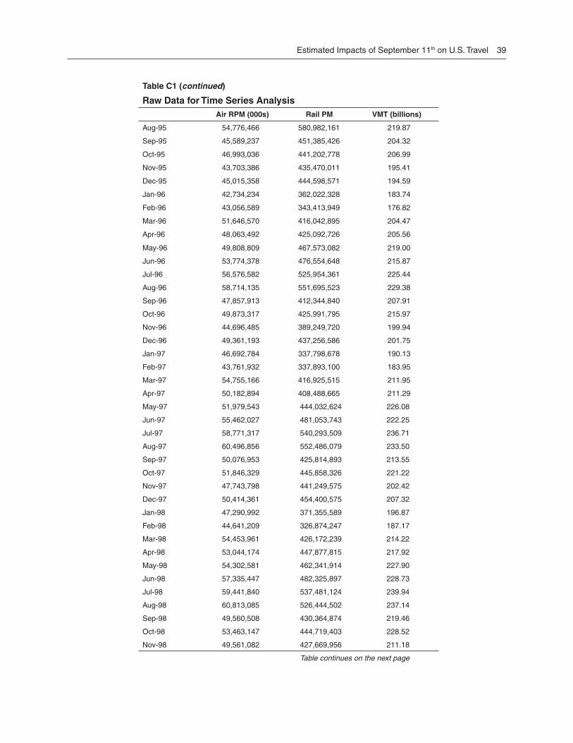
Estimated Impacts of September 11th on U.S. Travel 39
Table C1 (continued)
Raw Data for Time Series AnalysisAir RPM (000s) Rail PM VMT (billions)
Aug-95 54,776,466 580,982,161 219.87
Sep-95 45,589,237 451,385,426 204.32
Oct-95 46,993,036 441,202,778 206.99
Nov-95 43,703,386 435,470,011 195.41
Dec-95 45,015,358 444,598,571 194.59
Jan-96 42,734,234 362,022,328 183.74
Feb-96 43,056,589 343,413,949 176.82
Mar-96 51,646,570 416,042,895 204.47
Apr-96 48,063,492 425,092,726 205.56
May-96 49,808,809 467,573,082 219.00
Jun-96 53,774,378 476,554,648 215.87
Jul-96 56,576,582 525,954,361 225.44
Aug-96 58,714,135 551,695,523 229.38
Sep-96 47,857,913 412,344,840 207.91
Oct-96 49,873,317 425,991,795 215.97
Nov-96 44,696,485 389,249,720 199.94
Dec-96 49,361,193 437,256,586 201.75
Jan-97 46,692,784 337,798,678 190.13
Feb-97 43,761,932 337,893,100 183.95
Mar-97 54,755,166 416,925,515 211.95
Apr-97 50,182,894 408,488,665 211.29
May-97 51,979,543 444,032,624 226.08
Jun-97 55,462,027 481,053,743 222.25
Jul-97 58,771,317 540,293,509 236.71
Aug-97 60,496,856 552,486,079 233.50
Sep-97 50,076,953 425,814,893 213.55
Oct-97 51,846,329 445,858,326 221.22
Nov-97 47,743,798 441,249,575 202.42
Dec-97 50,414,361 454,400,575 207.32
Jan-98 47,290,992 371,355,589 196.87
Feb-98 44,641,209 326,874,247 187.17
Mar-98 54,453,961 426,172,239 214.22
Apr-98 53,044,174 447,877,815 217.92
May-98 54,302,581 462,341,914 227.90
Jun-98 57,335,447 482,325,897 228.73
Jul-98 59,441,840 537,481,124 239.94
Aug-98 60,813,085 526,444,502 237.14
Sep-98 49,560,508 430,364,874 219.46
Oct-98 53,463,147 444,719,403 228.52
Nov-98 49,561,082 427,669,956 211.18
Table continues on the next page

40 Estimated Impacts of September 11th on U.S. Travel
Table C1 (continued)
Raw Data for Time Series AnalysisAir RPM (000s) Rail PM VMT (billions)
Dec-98 51,024,977 459,051,399 216.30
Jan-99 48,861,094 384,824,724 194.44
Feb-99 46,158,194 350,270,063 192.33
Mar-99 57,761,057 436,837,107 221.74
Apr-99 54,968,382 435,360,347 221.98
May-99 55,469,960 450,054,655 231.81
Jun-99 59,918,608 496,553,598 237.02
Jul-99 64,397,523 543,923,323 244.20
Aug-99 63,752,132 528,001,216 242.57
Sep-99 53,733,696 393,137,094 225.30
Oct-99 57,407,208 425,897,553 234.66
Nov-99 53,866,781 421,595,015 222.83
Dec-99 52,331,272 442,742,459 222.46
Jan-00 49,745,428 366,607,410 203.58
Feb-00 49,876,910 366,139,276 199.64
Mar-00 61,378,569 453,096,388 232.63
Apr-00 58,981,617 473,751,011 227.81
May-00 61,165,486 481,725,263 242.11
Jun-00 65,524,091 517,102,460 243.01
Jul-00 67,883,256 564,747,276 245.08
Aug-00 66,924,512 558,060,051 247.77
Sep-00 56,441,629 446,489,429 227.33
Oct-00 58,834,210 462,329,685 236.55
Nov-00 56,283,261 442,268,378 222.80
Dec-00 55,380,280 461,651,082 218.44
Jan-01 53,129,922 379,458,113 209.26
Feb-01 49,992,995 366,288,212 199.91
Mar-01 62,323,049 448,912,584 231.49
Apr-01 59,801,562 455,496,342 231.37
May-01 60,246,477 462,376,555 244.25
Jun-01 64,987,625 528,690,495 242.58
Jul-01 68,573,410 564,037,290 248.79
Aug-01 69,003,617 562,266,005 251.69
Sep-01 39,106,905 446,266,947 224.57
Oct-01 44,271,037 452,095,235 240.00
Nov-01 45,245,063 446,094,295 229.48
Dec-01 48,167,518 479,188,434 228.09
Jan-02 46,587,818 398,440,459 213.81
Feb-02 45,157,533 397,948,828 206.46
Mar-02 57,423,155 461,087,451 234.01
Table continues on the next page

Estimated Impacts of September 11th on U.S. Travel 41
Table C1 (continued)
Raw Data for Time Series AnalysisAir RPM (000s) Rail PM VMT (billions)
Apr-02 53,013,066 453,147,413 234.81
May-02 55,663,570 461,648,459 249.89
Jun-02 60,224,150 499,751,748 246.39
Jul-02 62,570,110 564,046,073 254.19
Aug-02 62,881,793 516,103,068 256.24
Sep-02 48,925,997 385,097,846 230.60
Oct-02 52,779,975 399,248,774 243.29
Nov-02 48,902,677 375,996,408 228.39
Dec-02 55,355,434 448,246,102 231.26
Jan-03 50,602,700 393,287,373 216.60
Feb-03 46,455,943 390,041,481 201.90
Mar-03 56,033,121 472,573,962 236.70
Apr-03 51,146,721 483,653,074 238.10
May-03 53,591,384 489,484,678 253.20
Jun-03 59,426,357 531,138,943 252.00
Jul-03 65,041,408 578,767,927 261.30
Aug-03 64,095,456 557,897,322 259.60
Sep-03 51,347,366 427,807,444 236.00
Oct-03 55,810,667 463,025,617 253.40
Nov-03 53,249,129 448,181,812 233.30
Dec-03 57,795,908 489,403,554 237.60
Jan-04 53,447,972 410,338,691 217.30
Feb-04 52,608,801 389,778,365 210.40
Mar-04 63,600,019 453,014,590 247.50
Apr-04 61,887,720 471,116,666 245.40
May-04 62,074,299 472,861,212 253.00
Jun-04 67,833,476 514,365,919 253.70


43
APPENDIX D The Structural Time Series Model
Although terms such as “trend” and “seasonal” are intuitively appealing, they are mental constructs as we cannot observe them directly. Therefore, we use a structural modeling approach that treats them as unobserved components (Har-vey, 1989; Harvey and Shephard, 1993). In the empirical work we used the STAMP (Structural Time Series Analyser, Modeller and Predictor) software in conjunction with GiveWin; for details, see Koopman et al. (2000).
We defi ne the components at time t as follows: trend = µt; slope = βt; seasonal component = γt; and irregular component = εt. We assume that the process is observed at unit time intervals (t, t+1,…) and that there are s such intervals in a year (e.g. s=12 for monthly data). We then allow each component to evolve over time according to the specifi cations:
tttt ηβµµ ++= −− 11 (1)
ttt ςββ += −1 (2)and
tsttt ωγγγ =+++ +−− 11 .... (3)The quantities ηt, ζt, and ωt represent zero mean, random shifts in the cor-responding component. We assume such shifts to be independent of one an-other and uncorrelated over time; we also assume that they are independent of the “irregular” component, εt, seen in Equation (4) below. Equations (1)–(3) are known as the state or transition equations since they describe the underly-ing states of the process, or the transition of the components from one time period to the next.
Equations (1) and (2) provide a general framework for describing the evolu-tion of the trend. If the process being modeled does not require all of these

44 Estimated Impacts of September 11th on U.S. Travel
components, they can be dropped from the specifi cation. The components are tested in sequential fashion as follows (Harvey, 1989, pp. 248-56):
Does the slope disturbance term have positive variance? [Zero variance cor-responds to the slope being fi xed over time]
Does the level disturbance have positive variance? [Zero variance corresponds to the mean level being fi xed over time]
If the slope disturbance is dropped, does the slope differ from zero?
If all three statistical tests produced negative outcomes, the trend term would be reduced to a constant.
When the time series is seasonal, we check:
Does the seasonal disturbance term have positive variance? [Zero variance corre-sponds to a stable seasonal pattern]
If the seasonal disturbance is dropped, are the seasonal components signifi -cantly different from zero? [Is there any seasonal pattern?]
If we drop the seasonal disturbance term, we are left with a “classical” model with fi xed seasonal components. If the seasonal pattern is rejected completely, we reduce the model purely to its trend components.
The observed series is related to the states of the system by the observation (or measure-ment) equation:
tttty εγµ ++= (4) where εt denotes the ‘irregular’ component.
•
•
•
•
•
The irregular component has zero mean and is assumed to be serially uncorrelated (i.e., not predictable) and independent of the disturbances in the state equations.
Estimation proceeds by maximum likelihood (Harvey, 1989, pp. 125-128). Operational details are provided in Koopman et al. (2000, section 8.3). The key parameters are the four variances corresponding to the disturbance terms [σε
2, ση2, σζ
2 and σω
2]. Note that we assume these variances are constant over time; the time series may need to be trans-formed to justify this assumption, at least to a reasonable degree of approximation. The four variance terms control the form of the model, allowing each of level, slope and seasonal to be stochastic or fi xed; slope and seasonal elements may be present or absent. Table D1 illustrates the principal variations. If fi xed components are included in a model, the corresponding terms appear in the state equations (e.g. fi xed seasonal coeffi cients) but the variance term is zero. If the compo-nents are stochastic, the same terms appear in the model, but the variance is strictly positive. The most general form is the Basic Structural Model (BSM), in which all com-ponents are stochastic. The BSM forms the starting point for the model development process, and is the standard form employed in STAMP. The program then “tests down” to eliminate any components that are not required.

Estimated Impacts of September 11th on U.S. Travel 45
Table D1: Some of the Principal Models in the Structural Framework
Type of model σε2 ση
2 σζ2 σω
2
Level only
Constant mean yes 0 0 0
Local level (LL) yes yes 0 0
Random walk (RW) 0 yes 0 0
Trend only
Deterministic yes 0 0 0
Local level with fi xed slope yes yes 0 0
Random walk with fi xed drift 0 yes 0 0
Local linear trend (Holt) yes yes yes 0
Smooth trend yes 0 yes 0
Second difference 0 0 yes 0
Seasonal (with selected trend)
Fixed seasonals (yes or 0) (yes or 0) (yes or 0) 0
Varying seasonals (yes or 0) (yes or 0) (yes or 0) yes
Basic Structural Model (BSM) yes yes yes yes
NOTE: Based on Koopman et al. (2000), page 141.


47
APPENDIX E Summary of Monthly Forecasts
Table E1: Forecasts and Forecast Errors for Air RPMAir RPM Forecast of Air RPM before 9/11-01 Forecast error Absolute percent error
Mar-01 62,323,049
Apr-01 59,801,562
May-01 60,246,477
Jun-01 64,987,625
Jul-01 68,573,410
Aug-01 69,003,617
Sep-01 39,106,905 58,390,903.80 19,283,998.80 49.31%
Oct-01 44,271,037 61,261,140.50 16,990,103.50 38.38%
Nov-01 45,245,063 58,337,950.00 13,092,887.00 28.94%
Dec-01 48,167,518 57,977,550.10 9,810,032.10 20.37%
Jan-02 46,587,818 55,752,782.90 9,164,964.90 19.67%
Feb-02 45,157,533 52,754,058.80 7,596,525.80 16.82%
Mar-02 57,423,155 64,478,755.60 7,055,600.60 12.29%
Apr-02 53,013,066 61,791,637.40 8,778,571.40 16.56%
May-02 55,663,570 62,679,059.30 7,015,489.30 12.60%
Table E2: Forecasts and Forecast Errors for Rail RPMRail PM Forecasts of Rail PM before 9-11-01 Forecast error Absolute percent error
Mar-01 448,912,584
Apr-01 455,496,342
May-01 462,376,555
Jun-01 528,690,495
Jul-01 564,037,290
Aug-01 562,266,005
Sep-01 446,266,947 442,469,757.70 -3,797,189.30 0.85%
Oct-01 452,095,235 463,447,212.30 11,351,977.30 2.51%
Nov-01 446,094,295 448,090,467.10 1,996,172.10 0.45%
Dec-01 479,188,434 472,451,381.90 -6,737,052.10 1.41%
Jan-02 398,440,459 392,260,011.50 -6,180,447.50 1.55%
Feb-02 397,948,828 379,067,383.20 -18,881,444.80 4.74%
Mar-02 461,087,451 462,607,735.60 1,520,284.60 0.33%
Apr-02 453,147,413 472,183,198.80 19,035,785.80 4.20%
May-02 461,648,459 478,159,689.20 16,511,230.20 3.58%

48 Estimated Impacts of September 11th on U.S. Travel
Table E3: Forecasts and Forecast Errors for VMTVMT Forecast of VMT prior to 9-11-01 Forecast error Absolute percent error
Mar-01 231.49
Apr-01 231.37
May-01 244.25
Jun-01 242.58
Jul-01 248.79
Aug-01 251.69
Sep-01 224.57 232.25 7.67 3.42%
Oct-01 240.00 240.33 0.33 0.14%
Nov-01 229.48 225.79 -3.69 1.61%
Dec-01 228.09 226.04 -2.05 0.90%
Jan-02 213.81 212.42 -1.38 0.65%
Feb-02 206.46 205.80 -0.67 0.32%
Mar-02 234.01 236.01 2.01 0.86%
Apr-02 234.81 235.29 0.48 0.21%
May-02 249.89 247.92 -1.97 0.79%

49
REFERENCES
Dahl, Carol A. 1995. “Demand for Transportation Fuels: A Survey of Demand Elasticities and their Components,” Journal of Energy Literature, 1(2).
Harvey, Andrew C. 1989. Forecasting, Structural Time Series Models, and The Kalman Filter. Cambridge, UK: Cambridge University Press.
Harvey, Andrew C. and Neil Shephard.1993. “Structural Time Series Models.” In Handbook of Statistics, Volume 11. Edited by G.S. Maddala, C.R. Rao and H.D. Vinod. Amsterdam, The Netherlands: Elsevier Science.
Koopman, Siem Jan, Andrew C. Harvey, Jurgen A. Doornik and Neil Sheph-ard. 2000. STAMP: Structural Time Series Analyser, Modeller and Predictor. London: Timberlake Consultants Ltd.
Ord, Keith and Peg Young. 2004. “Estimating the Impact of Recent Interven-tions on Transportation Indicators”, Journal of Transportation and Statistics, Vol. 7, No. 1, pp.69-86.
Pindyck, Robert S., Daniel L. Rubinfeld. 1978. Econometric Models And Eco-nomic Forecasts. Lexington, Mass.: McGraw-Hill, 1st Edition.
