Washington University in St. LouisWashington University Open Scholarship

All Theses and Dissertations (ETDs)

January 2010

Essays on Money and Credit: A New MonetaristApproachDaniel SanchesWashington University in St. Louis

Follow this and additional works at: https://openscholarship.wustl.edu/etd

This Dissertation is brought to you for free and open access by Washington University Open Scholarship. It has been accepted for inclusion in AllTheses and Dissertations (ETDs) by an authorized administrator of Washington University Open Scholarship. For more information, please contactdigital@wumail.wustl.edu.

Recommended CitationSanches, Daniel, "Essays on Money and Credit: A New Monetarist Approach" (2010). All Theses and Dissertations (ETDs). 309.https://openscholarship.wustl.edu/etd/309

WASHINGTON UNIVERSITY IN ST. LOUIS

Department of Economics

Dissertation Examination Committee: Stephen Williamson, Chair

Gaetano Antinolfi Rodolfo Manuelli

James Bullard David Andolfatto Costas Azariadis

ESSAYS ON MONEY AND CREDIT: A NEW MONETARIST

APPROACH

by

Daniel Rocha Sanches

A dissertation presented to the Graduate School of Arts and Sciences

of Washington University in partial fulfillment of the

requirements for the degree of Doctor of Philosophy

May 2010 Saint Louis, Missouri

copyright by

Daniel Rocha Sanches

2010

 

  ii 

Abstract

Essays on Money and Credit: A New Monetarist Approach

Daniel R Sanches

Chapter 1: Money and Credit with Limited Commitment and Theft

Credit contracts and fiat money seem to be robust means of payment in the sense that we

observe both monetary exchange and credit transactions under a wide array of

technologies and monetary policy rules. However, a common result in a large class of

models of money and credit is that the optimal monetary policy -- usually the Friedman

rule -- eliminates any transactions role for credit: money drives credit out of the

economy. In this sense, money and credit are not robust in the model. We study the

interplay among imperfect recordkeeping, limited commitment, and theft, in an

environment that can support both monetary exchange and credit arrangements.

Imperfect recordkeeping makes outside money socially useful, but it also permits theft of

currency to go undetected, and therefore provides lucrative opportunities for thieves in

decentralized exchange. First, we show that imperfect recordkeeping and limited

commitment are not sufficient to account for the robust coexistence of money and credit.

Then, we show that theft, together with imperfect recordkeeping and limited

commitment, is sufficient to account for the robust coexistence, given that theft imposes a

cost on monetary exchange. The Friedman rule is in general not optimal with theft, and

the optimal money growth rate tends to rise as the cost of theft falls.

  iii 

Chapter 2: Unsecured Loans and the Initial Cost of Lending

We study the terms of credit in a competitive market where sellers are willing to

repeatedly finance the purchases of buyers by extending direct credit. Lenders (sellers)

can commit to deliver any long-term credit contract that does not result in a payoff that is

lower than that associated with autarky while borrowers (buyers) cannot commit to any

contract. A borrower's ability to repay a loan is privately observable. As a result, the

terms of credit within an enduring relationship change over time according to the history

of trades. Although there is free entry of lenders in the credit market, each lender has to

pay a cost to contact a borrower. We show that a lower cost makes each borrower better

off from the perspective of the contracting date, results in less variability in a borrower's

expected discounted utility, and makes each lender uniformly worse off ex post. As this

cost approaches zero, the credit contract offered by a lender converges to a full-insurance

contract.

Chapter 3: Costly Recordkeeping, Settlement System, and Monetary Policy

We study an arrangement in which the government provides a public settlement system

to the private sector and evaluate its implications for the implementation of monetary

policy. A key ingredient of the analysis is that it is costly for the government to operate a

record-keeping technology which is necessary for the construction of a settlement system

through which private loans and tax liabilities are settled. For this reason, the choice of

the optimal size of a settlement system by the government is non-trivial. Another benefit

  iv 

of such a system is that it allows the government to effectively control the money supply.

We show that the Friedman rule is suboptimal. Money and credit coexist as means of

payment at the optimum. The government relies on a credit system to implement an

optimal policy because of the role of credit in relaxing cash constraints. As a result,

money and credit are complementary in transactions: the existence of a credit system

makes the operation of a monetary system more effective.

  v 

Acknowledgements

I would like to thank my advisor Stephen Williamson for teaching me the modern theory of money and banking. His guidance and dedication were essential for the completion of this dissertation. I also would like to thank Gaetano Antinolfi, James Bullard, Rodolfo Manuelli, Costas Azariadis, David Andolfatto, Christopher Waller, Pedro Gomis-Porqueras, and Ping Wang for their helpful comments. I dedicate this dissertation to my wife Ammanda Sanches who supported me throughout my doctorate. Without her this project would not be possible.

  vi 

Table of Contents

Abstract Acknowledgements List of Figures Chapter 1 – Money and Credit with Limited Commitment and Theft References Chapter 2 – Unsecured Loans and the Initial Cost of Lending References Chapter 3 – Costly Recordkeeping, Settlement System, and Monetary Policy References

ii

v

vii

1

37

40

62

65

84

  vii 

List of Figures

Figure 1 – Efficiency when q** > q* Figure 2 – Efficiency when q** < q* Figure 3 – Equilibrium with Credit Figure 4 – Terms of Credit Figure 5 – Lender’s Cost Function

86

87

88

89

90

1 Money and Credit with Limited Commitmentand Theft1

1.1 Introduction

It is hard to �nd examples of economies in which we do not observe the use of both

money and credit in transactions. Thus, we should think of money and credit as

robust, in the sense that we will observe transactions involving both money and credit

under a wide array of technologies and monetary policy rules. One goal of this paper

is to help us understand what is required to obtain robustness of money and credit

in an economic model. Then, given robustness, we want to explore the implications

for monetary policy. As well, this paper will serve to tie together some key ideas in

monetary economics.

As is now well known, barriers to the �ow of information across locations and over

time appear to be critical to the role that money plays in exchange. If there were

no such barriers, in particular if there were perfect �memory�, i.e. recordkeeping,

then it would be possible to support e¢ cient allocations in the absence of valued

money �see Kocherlakota (1998). One can think of the models of Green (1987), or

Atkeson and Lucas (1992), as determining e¢ cient allocations with credit arrangements

under private information, where the memory of past transactions by economic agents

supports incentive compatible intertemporal exchange. As Kocherlakota (1998) points

out, spatial separation of the type encountered in turnpike models �such as Townsend

(1980) �or random matching models �such as Trejos and Wright (1995) �also yields

e¢ cient credit arrangements under perfect memory. Aiyagari and Williamson (1999)

study an environment with private information and random matching where credit

arrangements are e¢ cient. Thus, neither private information nor spatial separation

is a su¢ cient friction to provide a socially useful role for monetary exchange. Both

1Joint project with Stephen Williamson.

1

frictions mitigate credit arrangements, but not to the point where monetary exchange

necessarily improves matters.

The work of Kocherlakota (1996, 1998) seems to suggest that limited commitment

works much like private-information and spatial frictions, in that it in general implies

less intertemporal exchange than would occur in its absence, but does not imply a

welfare-improving role for money. However, in the case of limited commitment, this is

not obvious. For example, suppose that two economic agents, A and B meet. Agent

A can supply B with something that B wants, but all that B can o¤er in exchange is

a promise to supply A with some object in the future. Agent B is unable to commit,

and what A is willing to give to B will depend on A0s ability to punish B; or to have

other economic agents punish B; if he or she fails to ful�ll his or her promises in the

future. The amount of credit that A is willing to extend to B will in general be limited.

However, suppose that B has money to o¤er A in exchange. Possibly A and B can

trade more e¢ ciently using money, or by using money and credit, because monetary

exchange is not subject to limited commitment.

First, we wish to construct a framework which can potentially permit monetary

exchange, trade using credit under limited commitment, and the coexistence of valued

money and credit. We build on the model of Rocheteau and Wright (2005) and Lagos

and Wright (2005), which has quasilinear utility and alternating decentralized and

centralized trading among economic agents. This lends tractability to our analysis,

but we think that the basic ideas are quite general.

The �rst result is that, consistent with Kocherlakota (1998), limited commitment

is in fact not su¢ cient to provide a social role for money in our model. The result

hinges on the fact that lack of commitment applies to tax liabilities as well as private

liabilities. If there is perfect memory and limited commitment matters, then limited

commitment also may make the Friedman rule infeasible for the government. This is

2

because agents may want to default on the tax liabilities that are required to support

de�ation at the Friedman rule rate. While it is possible in special cases for money to

be valued in equilibrium with limited commitment and perfect memory, there is no

welfare-improving role for money. This is similar to the �avor of some results in the

monetary model without credit considered by Andolfatto (2008).

As mentioned above, one of our aims in this paper is to determine a set of frictions

under which money and credit are both robust as means of payment. Clearly, perfect

memory does not provide conditions under which monetary exchange is robust, so we

need to add imperfect memory to provide a role for money. However, we do not want

to shut down memory entirely, as is typical in some monetary models �e.g. Lagos and

Wright (2005) �as this will also shut down credit. We use a hybrid approach, whereby

decentralized meetings between buyers and sellers are either monitored, or are not. A

monitored trade is subject to perfect memory, while there is no access to memory in

non-monitored transactions �see also Deviatov and Wallace (2009).

In this context, our results depend critically on the punishments that are triggered

by default in the credit market. For tractability, we consider global punishments,

whereby default by a borrower will imply that all would-be lenders refuse to extend

credit. At the extreme, this can result in global autarky. With global autarky as an

o¤-equilibrium path supporting valued money and credit in equilibrium, higher money

growth lowers the rate of return on money, and there is substitution of credit for money.

E¢ cient monetary policy is either a Friedman rule, if incentive constraints do not bind

at the optimum, or else optimal money growth is greater than at the Friedman rule

and incentive constraints bind at the optimum. In either case, e¢ cient monetary policy

drives out credit. Money works so well that if the government gives money a su¢ ciently

high rate of return there will be no lending in equilibrium.

We also consider o¤-equilibrium punishments that are less severe than autarky.

3

Much as in Aiyagari and Williamson (2000) or in Antinol�, Azariadis, and Bullard

(2007), we allow punishment equilibria to include monetary exchange. That is, if

a borrower defaults, this triggers a global punishment where there is no credit, but

agents can trade money for goods. Here, the only equilibrium that can be supported

is one with no credit, and with a �xed stock of money (also implying a constant

price level in our model). This is quite di¤erent from results obtained in Aiyagari

and Williamson (2000) or Antinol�, Azariadis, and Bullard (2007). A key di¤erence

in our setup is that we take account of the fact that the government cannot commit

to punishing private agents through monetary policy. When a default occurs, the

government adjusts monetary policy so that it is a best response to the decision rules

that private agents adopt as punishment behavior.

Imperfect memory provides a role for money, but in the context of imperfect memory

alone, money in some sense works too well in our model, relative to what we see in

reality. That is, optimal monetary policy always drives credit out of the system. This

is a typical result, which is obtained for example in Ireland�s cash-in-advance model

of money and credit � see Ireland (1994). Ireland�s model has the property that a

Friedman rule is optimal and, at the Friedman rule, all transactions are conducted with

cash, which eliminates the costs of using credit. The intuition for this is quite clear.

All alternatives to using currency in transactions come at a cost, for example there are

costs of operating a debit-card or credit-card system, there are costs to clearing checks,

etc. If it is costless to produce currency and to carry it around, then if the government

generates a de�ation that induces a rate of return on money equivalent to that on the

best safe asset, then this should be e¢ cient, and it should also eliminate the use of all

cash substitutes in transactions.

Of course, in practice it is costly for the government to operate a currency system.

For example, maintaining the currency stock by printing new currency to replace worn-

4

out notes and coins is costly, as is counterfeiting and the prevention of counterfeiting.

As well, a key cost of holding currency is the risk of theft, which has been studied, for

example, in He, Huang, andWright (2008). We model theft di¤erently here, and do this

in the context of monitored credit transactions. That is, we assume that it is possible

for sellers, at a cost, to steal currency in non-monitored transactions, but theft is not

possible if the transaction is monitored. This changes our results dramatically. Now,

monetary policy will a¤ect the amount of theft in existence, and theft will matter for

how borrowers are punished in the event of default. For example, if the o¤-equilibrium

punishment path involves no credit market activity and only monetary exchange, then

the risk of theft is higher on the o¤-equilibrium path, and this reduces welfare in the

punishment equilibrium.

At the optimum it will always be optimal for the government to eliminate theft.

Theft will matter for policy, but in the model theft will not be observed in equilibrium.

Because theft is potentially more prevalent with o¤-equilibrium punishment, however,

money and credit will in general coexist at the optimum. When theft matters, the

Friedman rule is not optimal, and the optimal money growth rate tends to increase as

the cost of theft falls.

1.2 The Environment

Time is discrete and each period is divided into two subperiods: day and night. There

are two types of agents in the economy, buyers and sellers, and there is a continuum of

each type with unit measure. There is a unique perishable consumption good which is

produced and consumed within each subperiod. During the day, a seller can produce

one unit of the consumption good with one unit of labor. At night, a buyer is able to

produce one unit of the consumption good with one unit of labor.

5

A buyer has preferences given by

1Xt=0

�t[u (qt)� nt] (1.1)

where qt is consumption during the day, and nt is labor supply at night, with � 2 (0; 1)

the discount factor between night and day. Assume u(�) is strictly concave, strictly

increasing, and twice continuously di¤erentiable with u(0) = 0; u0(0) =1; and de�ne

q� to be the solution to u0(q�) = 1: A seller has preferences given by

1Xt=0

�t(�lt + xt) (1.2)

where lt is labor supply during the day and xt is consumption at night. Sellers and

buyers discount at the same rate. Agents are bilaterally and randomly matched during

the day and at night trade is centralized.

1.3 Planner�s Problem

1.3.1 Full Commitment

First, consider what a social planner could achieve in this economy in the absence of

money. Ultimately, money will consist of perfectly divisible and durable objects that

are portable at zero cost, and can be produced only by the government. In this section

assume there is complete memory and that each agent can commit to the plan proposed

by the social planner at t = 0: If the planner treats all sellers identically and all buyers

identically, then an allocation f(qt; xt)g1t=0 satis�es the participation constraints1Xt=0

�t[u (qt)� xt] � 0; (1.3)

and1Xt=0

�t(�qt + xt) � 0; (1.4)

which state that a buyer and a seller, respectively, each prefer to participate in the

plan at t = 0: Then, if we con�ne attention to stationary allocations with qt = q and

6

xt = x for all t; we must have

u (q)� x � 0 (1.5)

and

�q + x � 0 (1.6)

The set of feasible stationary allocations is given by (2.5) and (3.4), and this set

is non-empty given our assumptions. Further, the set of e¢ cient allocations is also

non-empty, satisfying (2.5), (3.4) and q = q�:

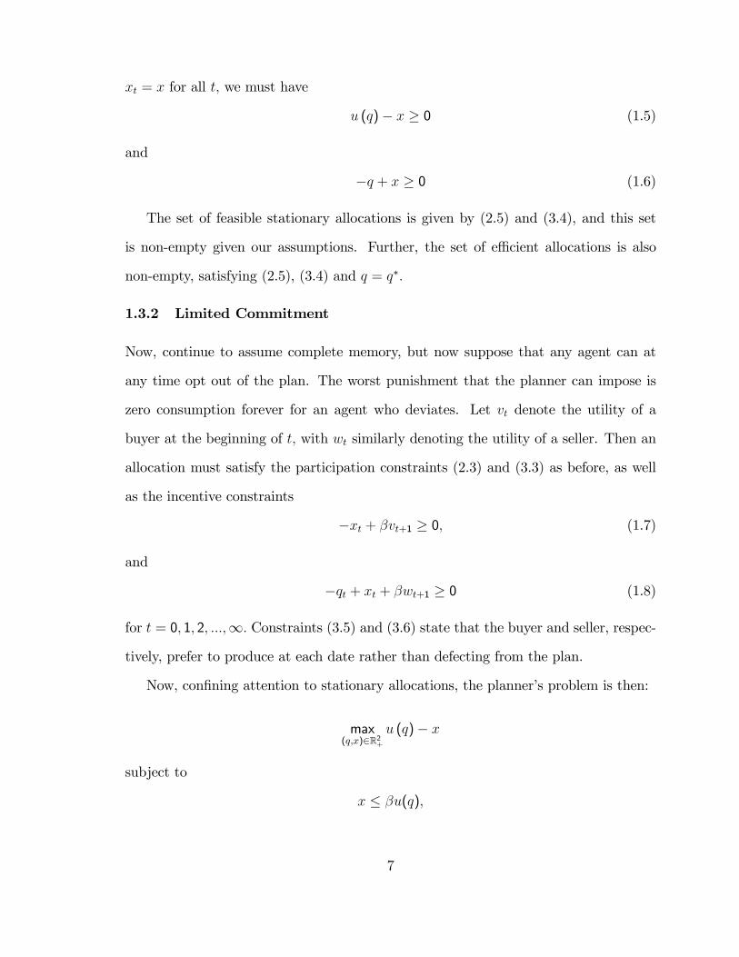
1.3.2 Limited Commitment

Now, continue to assume complete memory, but now suppose that any agent can at

any time opt out of the plan. The worst punishment that the planner can impose is

zero consumption forever for an agent who deviates. Let vt denote the utility of a

buyer at the beginning of t; with wt similarly denoting the utility of a seller. Then an

allocation must satisfy the participation constraints (2.3) and (3.3) as before, as well

as the incentive constraints

�xt + �vt+1 � 0; (1.7)

and

�qt + xt + �wt+1 � 0 (1.8)

for t = 0; 1; 2; :::;1: Constraints (3.5) and (3.6) state that the buyer and seller, respec-

tively, prefer to produce at each date rather than defecting from the plan.

Now, con�ning attention to stationary allocations, the planner�s problem is then:

max(q;x)2R2+

u (q)� x

subject to

x � �u(q);

7

and

�q + x � (1� �)w:

where w is the seller�s lifetime utility. At the optimum, the seller�s incentive constraint

binds, so that x = q + (1� �)w. Now, let q�� denote the solution to �u(q��) = q��:

We can then rewrite the buyer�s incentive constraint as

�u(q)� q � (1� �)w: (1.9)

Given that w � 0, we must have q 2 [0; q��]. Then, we can rewrite the planner�s

problem in the following way:

maxq2[0;q��]

u (q)� q � (1� �)w

subject to (3.7). The �rst-order conditions are

u0 (q)� 1 + � [�u0 (q)� 1] � 0; with equality if q < q��; (1.10)

and

� [�u(q)� q � (1� �)w] = 0;

where � � 0 is the Lagrange multiplier associated with the constraint (3.7).

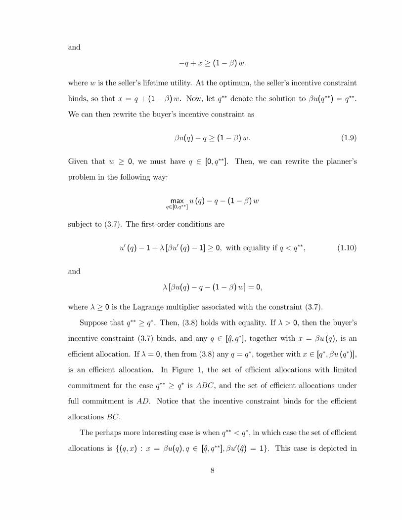
Suppose that q�� � q�. Then, (3.8) holds with equality. If � > 0, then the buyer�s

incentive constraint (3.7) binds, and any q 2 [q; q�], together with x = �u (q), is an

e¢ cient allocation. If � = 0, then from (3.8) any q = q�, together with x 2 [q�; �u (q�)],

is an e¢ cient allocation. In Figure 1, the set of e¢ cient allocations with limited

commitment for the case q�� � q� is ABC, and the set of e¢ cient allocations under

full commitment is AD. Notice that the incentive constraint binds for the e¢ cient

allocations BC.

The perhaps more interesting case is when q�� < q�; in which case the set of e¢ cient

allocations is f(q; x) : x = �u(q); q 2 [q; q��]; �u0(q) = 1g. This case is depicted in

8

Figure 2, where the set of e¢ cient allocations is AB: That is, in this case the incentive

constraint for the buyer always binds for the e¢ cient stationary allocation, and an

e¢ cient allocation with limited commitment is not e¢ cient under full commitment.

1.4 Equilibrium Allocations with Perfect Memory

To establish a benchmark, we �rst assume that there is perfect memory. As we would

expect from the work of Kocherlakota (1998), this will severely limit the role of money

in this economy. An important element of the model will be the bargaining protocol

carried out when a buyer and seller meet during the daytime. We assume that the

seller �rst announces whether or not he or she is willing to trade with the buyer. If

the seller is not willing to trade, then no exchange takes place. Otherwise, the buyer

then makes a take-it-or-leave-it o¤er to the seller. This protocol in part allows us to

focus on the limited commitment friction, as take-it-or-leave-it o¤ers imply that there

will be no bargaining ine¢ ciencies.

When a buyer and seller are matched during the day, they continue to be matched

at the beginning of the following night, after which all agents enter the nighttime

Walrasian market.

1.4.1 Credit Equilibrium

Ultimately we will want to determine the role for valued money in this perfect-memory

economy, but our �rst step will be to look at equilibria where money is not valued.

Here, the daytime take-it-or-leave-it o¤ers of buyers consist of credit contracts, with

a loan made during the day and repayment at night. We will con�ne attention to

stationary equilibria where sellers always choose to trade when they meet a buyer

during the day. Let l denote the loan quantity o¤ered by the buyer to the seller in the

day. Then, letting v denote the lifetime continuation utility of the buyer after repaying

9

the loan during the night, we have

v = �maxl[u(l)� l + v] (1.11)

subject to the incentive constraint

l � v � v;

and

l � 0:

Here, v is the buyer�s continuation utility if he or she defaults on the loan, which triggers

a punishment. In the equilibrium we consider here, v = 0; so that the punishment

for default is autarky for the defaulting buyer. On the o¤-equilibrium path, it is an

equilibrium for no one to trade with an agent who has defaulted as, if agent A trades

with agent B who has defaulted in the past, this triggers autarky for agent A. Here,

note that the individual punishment for a buyer who defaults is identical to a global

punishment whereby default by any buyer triggers global autarky. Letting c(v) denote

the right-hand side of (3.9), we get

c(v) = �u(v); for 0 � v � q�;

and

c(v) = � [u(q�)� q� + v] ; for v � q�:

An equilibrium is then a solution to v = c(v): If q�� < q� then there are two equilibria.

In the �rst, v = 0; and in the second v > 0; which are both solutions to v = �u(v): Note

that v is also the consumption of the buyer during the day, and of the seller during the

night, with v < q�: In this case, the incentive constraint for the buyer binds in either

equilibrium. If q�� � q� then the v = 0 equilibrium still exists, and the equilibrium

with v > 0 has

v =�

1� �[u(q�)� q�] ;

10

in which case consumption is q� for any agent consuming at any date and the incentive

constraint does not bind.

Note that, in equilibrium, a seller meeting a buyer during the daytime is always

indi¤erent to trading or not. If he or she announces a willingness to trade, then the

buyer makes an o¤er that leaves the seller with zero surplus, and utility is identical to

what the seller would have achieved without trade. In the equilibrium we study, the

seller always chooses to trade.

In Figure 3, panel (b) shows the case where the incentive constraint binds in equi-

librium, and panel (a) the case where the incentive constraint does not bind. The

nonmonetary credit equilibrium, by virtue of the bargaining solution we use, just picks

out the e¢ cient stationary allocation that gives all of the surplus to the buyer.

1.4.2 Monetary Equilibrium

Assume that money is uniformly distributed across buyers at the beginning of the �rst

day. Subsequently the government makes equal lump-sum transfers at the beginning

of the night to buyers, so that the money stock grows at the gross rate �: Con�ne

attention to stationary monetary equilibria, and consider only cases where � � �; as

otherwise a monetary equilibrium does not exist. Letm denote the real money balances

acquired by a buyer in the night, and the real value of a lump-sum transfer received

by a buyer from the government during the night. Suppose that the buyer receives

the lump-sum transfer before acquiring money balances during the night, and continue

to let v denote the continuation utility for the buyer after receiving the lump-sum

transfer. As in Andolfatto (2008), we treat the government symmetrically with the

private sector, in that there is limited commitment with respect to tax liabilities as

well as private liabilities.

Continue to assume complete memory and, as in the previous subsection, default

by a buyer triggers autarky for that buyer. Since a seller will always be indi¤erent to

11

trading with a buyer, sellers not only refuse to engage in credit contracts with a buyer

who has defaulted; they also refuse to take his or her money. Note that the trigger to

individual autarky is identical to a global punishment where, if an agent defaults, no

seller will trade with any buyer. With global punishment, the value of money is zero

on the o¤-equilibrium path.

In this case, we determine the continuation value v for the buyer by

v = maxl;m

��m+ �

�u

�1

�m+ l

�� l + + v

��(1.12)

subject to

l � + v � v

l � 0:

Again, we have v = 0: Here, note that we need to be careful about the lump-sum

transfer the buyer receives. Should the buyer default on his or her debt, he or she

will also not receive the transfer, or will default on current and future tax liabilities if

< 0: In equilibrium, we have

= m

�1� 1

�

�:

For � > �; the right-hand side of equation (3.10) is given by

m(v) = �v1 + �u(v1) + v; for max�0;m�

�1

�� 1��

� v � v1;

m(v) = �u(v); for v1 � v � q�;

m(v) = � [u(q�)� q� + v] ; for v � q�:

Here, m� solves

u0�m�

�

�=�

�;

and v1 satis�es

u0 (v1) =�

�;

12

For � = �; we have

m(v) = �[u(q�)� q�]�m(1� �) + �v; for v � m��1

�� 1�;

where

m 2 [q� �min(q�; v); �q�]:

Proposition 1 If q�� � q�; then a monetary equilibrium does not exist if � 6= �:

Proof. If � < �, a monetary equilibrium does not exist, for standard reasons.

Suppose � > �. De�ne the function � (v) = m (v)� v. Notice that � (�) is continuous

and limv!1 � (v) = �1. Moreover, � (v) > 0 for all v 2 [max f0; (1� �) v1g ; q�) and

� (�) is strictly decreasing on (q�;1). Hence, there exists a unique value v � q� such

that � (v) = 0. However, money is not valued in this equilibrium. Q.E.D.

Proposition 2 If q�� � q� and � = �; then a continuum of monetary equilibria ex-

ists with v 2 [�[u(q�)�q�]1�� � min

n�q�; �u(q

�)�q�1��

o; �[u(q

�)�q�]1�� ): All of these equilibria yield

expected utility for the buyer of u(q�)�q�1�� :

Proof. Suppose � = �. It follows that � (�) is continuous everywhere except possibly

at v = q� and limv!1 � (v) = �1. We have � (v) = �u (q�) � q� > 0 for all v 2

[(1� �) q�; q�). At v = q� we have � (q�) = �u (q�) � q� � (1� �)m. A necessary

condition for the existence of a monetary equilibrium is � (q�) � 0, which requires

m � �u (q�)� q�

1� �.

Hence, a necessary and su¢ cient condition for the existence of a monetary equilibrium

is

m � min��q�;

�u (q�)� q�

1� �

�.

13

Given a positive value of m satisfying the inequality above, there exists a unique value

v � q� such that � (v) = 0, in which case money is valued in equilibrium. Therefore,

there exists a continuum of monetary equilibria with

v 2 [�[u(q�)� q�]

1� ��min

��q�;

�u (q�)� q�

1� �

�;�[u(q�)� q�]

1� �).

All of these equilibria support the allocation (q; x) = (q�; q�). Q.E.D.

Proposition 3 If q�� < q�; then a monetary equilibrium does not exist if � 6= �u0(q��).

Proof. Suppose � > �u0 (q��). Notice that � (v) = �u (v1) � v1 > 0 for all v 2

[max f0; (1� �) v1g ; v1), � (v) > 0 for all v 2 [v1; q��), and � (q�) < 0. Since � (�) is

continuous and strictly decreasing on (q��;1), it follows that v = q�� is the unique

value satisfying � (v) = 0. Since v1 < q��, it follows that money is not valued in

equilibrium. Suppose � 2 (�; �u0 (q��)). In this case, � (v) < 0 for all v � (1� �) v1,

so that a monetary equilibrium does not exist. Finally, assume � = �. Again, we �nd

that � (v) < 0 for all v � (1� �) q�, so that a monetary equilibrium does not exist.

Q.E.D.

Proposition 4 If q�� < q� and � = �u0(q��); then a continuum of monetary equilibria

exists with v 2 [q�� [1� �u0 (q��)] ; q��): All of these equilibria yield expected utility for

the buyer of u(q��)�q��1�� :

Proof. Take � = �u0(q��). Then, � (v) = 0 for all v 2 [q�� [1� �u0 (q��)] ; q��] and

� (v) < 0 for all v > q��. Hence, a continuum of monetary equilibria exists with v 2

[q�� [1� �u0 (q��)] ; q��). All of these equilibria yield the allocation (q; x) = (q��; q��).

Q.E.D.

If the money growth rate is su¢ ciently high, that is if � > �max[1; u0(q��)]; then

the rate of return on money is su¢ ciently low that money is not held in equilibrium.

14

If q� � q��; it certainly seems clear why a monetary equilibrium will not exist when

the money growth rate is su¢ ciently high. In this case, when money is not valued a

credit equilibrium exists which is e¢ cient and incentive constraints do not bind. Thus,

there is clearly no role for money in equilibrium in relaxing incentive constraints in

decentralized trade. Why money is not valued even when q� > q�� and � > �u0(q��)

is perhaps less clear. In this case, the only stationary equilibria that exist are the

two credit equilibria: one where v = 0 and one with v > 0 and binding incentive

constraints, as in Figure 3. Money cannot relax the binding incentive constraints, as

in order to support a money growth rate su¢ ciently low as to induce agents to hold

money, the government would have to impose su¢ ciently high taxes that buyers would

choose to default on their tax liabilities. Thus, there is no role for money in improving

e¢ ciency.

If � = �max[1; u0(q��)]; then in equilibrium buyers are essentially indi¤erent be-

tween using money and credit in decentralized transactions with sellers, and there

exist a continuum of equilibria with valued money. Each of these equilibria supports

the same allocation as does the credit equilibrium with v > 0: The continuum of equi-

libria is indexed by the quantity of real money balances held by buyers. Across these

equilibria, as the quantity of real balances rises, the quantity of lending falls.

Our results are consistent with the ideas in Kocherlakota (1998), as they should

be. With perfect memory, money is not socially useful. At best, money can be held in

equilibrium. This equilibrium is either one where incentive constraints do not bind and

the monetary authority follows a Friedman rule, or incentive constraints bind and the

money growth rule is similar to what Andolfatto (2008) �nds. In either case, money

provides no e¢ ciency improvement.

15

1.5 Imperfect Memory and Autarkic Punishment

As we have seen, with perfect memory there is essentially no social role for money, and

it will only be held under special circumstances. As is well known, particularly given the

work of Kocherlakota, we need some imperfections in record-keeping in order for money

to be useful and to help it survive as a valued object. We will start by assuming that,

during the day, there is no memory in some bilateral meetings, and perfect memory

in other meetings. In particular, a fraction � of sellers has no monitoring potential,

while a fraction 1 � � does. In any day, a given buyer has probability � of meeting a

seller with no monitoring potential, in which case there is no memory in the interaction

between the buyer and seller. That is, each agent in such a meeting has no knowledge

of his or her trading partner�s history, and nothing about the meeting will be recorded.

With probability 1� � a buyer meets a seller with monitoring potential. In this case,

the buyer has the opportunity to choose to have his or her interaction with the seller

monitored. Here, 0 < � � 1: If the buyer chooses a monitored interaction in the day,

then his or her history is observable to the seller, and the interaction between that

buyer and seller will be publicly observed during the day and through the beginning of

the following night. Otherwise, the buyer�s and seller�s actions are unobserved during

the day and the following night.

Trade is carried out anonymously in the Walrasian market that opens in the latter

part of each night, in the sense that all that can be observed in the Walrasian market

is the market price. Individual actions are unobservable. Here, the case where � = 1 is

the standard one in monetary models with random matching such as Lagos and Wright

(2005). However, even in the case with � = 1; we deviate from the usual assumptions,

in that there is lack of commitment with respect to tax liabilities. We assume that

each agent can observe the interaction between the government and all other agents.

That is, default on tax liabilities is publicly observable.

16

We change the bargaining protocol between a buyer and seller during the day as

follows. The buyer �rst declares whether interactions with the seller during the period

will be monitored or not. If monitoring is chosen, then the seller learns the buyer�s

history of publicly-recorded transactions. Then, the seller decides whether or not to

transact with the buyer. If the seller is willing to transact, the buyer then makes a

take-it-or-leave-it o¤er.

Given our setup, if a buyer defaults on a loan made in a monitored trade, this will be

public information. As well, default by a buyer on tax liabilities is public information.

However, suppose that a seller were to make a loan to a buyer during the day in a non-

monitored trade, and then the buyer defaulted on the loan during the night. In this

case, it is impossible for that seller to signal to anyone else that default has occurred.

The interaction between the buyer and seller is private information, and the individual

seller cannot a¤ect prices in any subsequent nighttime Walrasian market. Further, in

the equilibria we study, a seller in a non-monitored trade during the day will never

have the opportunity to engage in a monitored trade during any subsequent day and

so will be unable to signal that a default has occurred.

1.5.1 Credit Equilibrium

First consider stationary equilibria where money is not valued, so that all exchanges

in the day market involve credit. Here, in the case where a buyer does not have the

opportunity to engage in a monitored transaction, there will be no exchange between

the buyer and the seller, as the buyer will be able to default and this will be private

information. Thus if money is not valued, then trade takes place during the day only in

monitored transactions, and the buyer will always weakly prefer to have the interaction

with a seller monitored. Here, v is determined by

v = �n(1� �)max

l[u(l)� l] + v

o(1.13)

17

subject to the incentive constraint

l � v � v;

and

l � 0:

As in the previous section, v is the continuation value when punishment occurs, and

the punishment is autarky so v = 0. Now, letting �c(v) denote the right-hand side of

(2.13), we can rewrite (2.13) as

v = �c(v);

with

�c(v) = � [(1� �)u(v) + �v] ; for 0 � v � q�

and

�c(v) = � f(1� �)[u(q�)� q�] + vg ; for v � q�:

Let q��� denote the solution to

�(1� �)

1� ��u(q���) = q���

Proposition 5 If q��� < q� then there are two credit equilibria, one where v = 0; and

one where the incentive constraint binds, l < q� and v = q���:

Proof. De�ne �c (v) = �c (v)� v. Note that �c (�) is continuous and limv!1 �c (v) =

�1. Since q��� < q�, it follows that �c (v) > 0 for all v 2 (0; q���), �c (q���) = 0, and

�c (v) < 0 for all v 2 (q���;1). This implies that v = q��� is the unique positive value

satisfying �c (v) = 0. Since the incentive constraint binds, it follows that l = q��� in

such equilibrium. Q.E.D.

Proposition 6 If q��� � q� then there are two credit equilibria, one where v = 0 and

one where the incentive constraint does not bind, l = q�; and

v =�(1� �)[u(q�)� q�]

1� �:

18

Proof. In this case, �c (v) > 0 for all v 2 (0; q�) and �c (q�) � 0. Note that �c (�) is

strictly decreasing on (q�;1), with limv!1 �c (v) = �1. Hence, there exists a unique

positive value v � q� satisfying �c (v) = 0. This means that

� f(1� �) [u (q�)� q�] + vg � v = 0,

so that

v =� (1� �)

1� �[u (q�)� q�] ,

and l = q� is the amount consumed by the buyer in a monitored meeting during the

day. Q.E.D.

Now, since q��� < q�� for � > 0; imperfect memory limits credit market activity, just

as one might expect. Relative to the credit equilibrium with perfect memory there is

in general less trade in a credit equilibrium with imperfect memory, and the quantity

traded decreases as � increases. Of course, there is no credit market activity when

� = 1:

1.5.2 Monetary Equilibrium

As in the previous section, publicly observable default triggers autarky for the agent

who defaults. However, in this case autarkic punishment is carried out through a global

punishment whereby, if a single buyer defaults, this triggers an equilibrium where no

seller will trade during the day and therefore money is not valued.

Here, we solve for the equilibrium continuation value in a similar fashion to the

previous section. That is,

v = maxm;l

��m+ �

��u

�m

�

�+ (1� �)

�u

�m

�+ l

�� l

�+ + v

��(1.14)

subject to

l � + v � v;

19

l � 0:

Given autarkic punishment, v = 0: In equilibrium, the real value of the government

transfer is

= m

�1� 1

�

�: (1.15)

Here, and in the rest of the paper, it will prove to be more straightforward to de�ne

an equilibrium and solve for it in terms of the consumption quantities for the buyer in

non-monitored and monitored trades, rather than solving for the continuation value v:

Therefore, let x be the daytime consumption of a buyer in the non-monitored state,

and y the buyer�s daytime consumption in the monitored state. Then in the problem

(2.14) above, we have m = �x; = x(�� 1); and l = y � x: Thus from (2.14), we can

solve for v in terms of x and y to get

v = ��x+ � f� [u(x)� x] + (1� �) [u(y)� y]g1� �

:

We can then de�ne an equilibrium in terms of x and y as follows.

De�nition 1 A stationary monetary equilibrium is a pair (x; y), where x and y are

chosen optimally by the buyer,

�u0 (x) + (1� �)u0 (y) =�

�, (1.16)

x and y have the property that consumptions and the loan quantity are nonnegative,

and consumptions do not exceed the surplus-maximizing quantity,

0 � x � y � q�, (1.17)

and (x; y) is incentive compatible,

� [�u (x) + (1� �)u (y)]� ��x� (1� ��) y � (1� �)v, (1.18)

where y = q� if (1.18) does not bind.

20

Proposition 7 If q�� � q� then a unique stationary monetary equilibrium exists for

� � �.

Proof. Suppose q� � q��� � q��. In this case, we cannot have an equilibrium with

a binding incentive constraint. Now, if the incentive constraint does not bind, then

y = q� and

�u0 (x) + 1� � =�

�. (1.19)

Note that (1� �) �u (q�) � (1� ��) q� � 0, so that the incentive constraint is always

slack when y = q�. Therefore, a unique stationary monetary equilibrium with a non-

binding incentive constraint exists for any � � �, with x de�ned by (1.19) and y = q�.

Suppose q��� < q� � q��. First, assume the incentive constraint does not bind.

Then, there exists ~� > � such that

�� [u (x)� x] � � (1� �) �u (q�) + (1� ��) q�

if and only if � 2 [�; ~�]. Again, a unique stationary monetary equilibrium with a

non-binding incentive constraint exists for � 2 [�; ~�]. Let ~x be the value of x satisfying

(1.19) when � = ~�. For � > ~�, the incentive constraint binds, and a unique stationary

monetary equilibrium exists with (x; y) satisfying

�� [u (x)� x] = � (1� �) �u (y) + (1� ��) y (1.20)

and

�u0 (x) + (1� �)u0 (y) =�

�, (1.21)

where x < ~x and q��� < y < q�. Q.E.D.

Proposition 8 If q�� < q� then a unique stationary monetary equilibrium exists for

� � �u0(q��):

21

Proof. Note that we cannot have an equilibrium with a non-binding incentive

constraint because

�� [u (x)� x] < � (1� �) �u (q�) + (1� ��) q�

when q�� < q�. Then, (x; y) satisfy (1.20) and (1.21), with 0 � x � y < q�. Note that

(1.20) requires that y � q��. Then, a unique stationary monetary equilibrium exists

for any � � �u0 (q��). Q.E.D.

If q��� � q�; which guarantees that q�� > q�; as q��� < q��; then the incentive

constraint does not bind for all � � �: In this case, the buyer consumes q� in all

monitored trades where credit is used during the day, and consumes x in non-monitored

trades, where x � q� and x is decreasing in �: Therefore, the welfare of the buyer is

decreasing in �; while the seller receives zero utility in each period for all �: Further,

when � = �; then x = y = q�; in which case the loan quantity is l = y � x = 0; and

no credit is used. As � increases, then, the quantity of credit rises, that is credit is

substituted for money in transactions.

If q�� � q� > q���; then the incentive constraint binds for � > ~�; where

�� [u (~x)� ~x] = ��(1� �)u(q�) + (1� ��)q�

with ~x the solution to

�u0 (~x) + 1� � =~�

�:

The incentive constraint does not bind for � � � � ~�: Here, � = � implies that

x = y = q� and there is no credit, just as in the previous case. However, if the money

growth rate is su¢ ciently high, then the incentive constraint binds. If the incentive

constraint does not bind, then just as in the previous case y = q� and x falls as � rises,

so that the welfare of buyers falls with an increase in � and credit is substituted for

money in transactions. If the incentive constraint binds, then it is straightforward to

22

show that an increase in � causes both x and y to fall, with the loan quantity l = y�x

increasing. Thus, as in the other cases, the welfare of buyers must fall as � rises, and

the use of credit rises with an increase in the money growth rate.

Finally, if q�� < q�; then the incentive constraint will always bind in a stationary

monetary equilibrium. Here, when � = �u0(q��); then x = y = q�� and there is

no credit. Again, it is straightforward to show that x, y; and the welfare of buyers

decrease with an increase in �; and the quantity of lending rises.

Which case we get (the incentive constraint never binds; the incentive constraint

binds only for large money growth rates; the incentive constraint always binds) depends

on q�� q���:While q� is independent of � and �; q��� is increasing in � and decreasing

in �: Thus, the incentive constraint will tend to bind the lower is � and the higher is

�: Higher � tends to relax incentive constraints for typical reasons. That is, as buyers

care more about the future, potential punishment is more e¤ective in enforcing good

behavior. Higher � implies that the imperfect memory friction becomes more severe,

and credit can be used with lower frequency. In general, monetary exchange will be less

e¢ cient than credit, and so a reduction in the frequency with which credit can be used

will tend to reduce the utility of a buyer in equilibrium. This will therefore reduce

the relative punishment to a buyer if he or she defaults and thus tighten incentive

constraints.

Proposition 9 If q�� � q�; then � = � is optimal, and this implies that l = 0, the

incentive constraint does not bind, and the buyer consumes q� in all trades during the

day.

Proof. Suppose the government treats buyers and sellers equally. Then, the govern-

ment chooses a money growth rate � � � to maximize � [u (x)� x]+(1� �) [u (y)� y]

subject to (2.16), (2.17), and (1.18). It follows that � = � implies x = y = q�, and the

e¢ cient allocation under full commitment is implemented. Q.E.D.

23

Proposition 10 If q�� < q�; then � = �u0(q��) is optimal, and this implies that l = 0;

the incentive constraint binds, and the buyer consumes q�� in all trades during the day.

Proof. If q�� < q�, the incentive constraint requires that y � q��. It follows from

(1.20) and (1.21) that setting � = �u0(q��) implements the e¢ cient allocation (q��; q��).

Q.E.D.

Here, we have essentially generalized the results of Andolfatto (2008) to the case

where credit is permitted in some types of bilateral trades. If the discount factor is

su¢ ciently small, then the Friedman rule is not feasible and the incentive constraint

binds at the optimum. In terms of our goal of constructing a model with robust money

and credit, an undesirable feature of this setup is that optimal monetary policy drives

credit out of the economy. Here, the only ine¢ ciency in monetary exchange is due

to the fact that buyers in general hold too little real money balances in equilibrium,

and this ine¢ ciency can be corrected in the usual way, with the caveat that too much

de�ation can cause agents to default on their tax liabilities. Ultimately, at the optimum

money is equivalent to memory, in that an appropriate monetary policy achieves the

same allocation that could be achieved by a social planner with perfect recordkeeping.

1.6 Imperfect Memory and Non-Autarkic Punishment

In the previous section, given the limited commitment friction, optimal monetary policy

will yield an equilibrium allocation where credit is not used. Credit seems to be more

robust than this in practice, so we would like to study frictions that potentially imply

that money and credit coexist, even when monetary policy is e¢ cient.

Here, we will assume the same information technology and bargaining protocol

as in the previous section. However, we will consider a di¤erent equilibrium, where

default does not trigger autarky, but instead triggers an equilibrium where money is

valued. That is, a default results in reversion to an equilibrium where sellers will not

24

trade if a buyer announces that he or she wishes the interaction to be monitored,

but will exchange goods for money if the buyer announces that the interaction will

not be monitored. The government is not able to commit to a monetary policy, so

the money growth rate that is chosen by the government when punishment occurs is

chosen optimally at that date given the behavior of private sector agents.

We restrict attention to punishment equilibria that are stationary. Further, a pun-

ishment equilibrium must be sustainable, in that no agent would choose to default on

his or her tax liabilities in such an equilibrium. Letting v denote the continuation value

in the punishment equilibrium, after agents receive their lump-sum transfers from the

government, we have

v = �m(�) + �

�u

�m(�)

�

�+m(�)

�1� 1

�

�+ v

�where m(�) is the quantity of real balances acquired by the buyer during the night,

which solves the �rst-order condition

u0�m(�)

�

�=�

�: (1.22)

Now, for the punishment equilibrium to be sustainable, we require that

m(�)

�1� 1

�

�+ v � v; (1.23)

i.e. the equilibrium is sustained in the sense that, if an agent chooses not to accept

the transfer from the government, then the punishment is reversion to the punishment

equilibrium. Clearly, condition (1.23) implies that punishment equilibria are sustain-

able if and only if � � 1: That is, private agents need to be bribed to enforce the

punishment with positive transfers, otherwise they would default on the tax liabilities.

The government will choose � optimally in the punishment equilibrium, and it must

choose a sustainable money growth factor, i.e. � � 1: Assume that the government

weights the utility of buyers and sellers equally, though since sellers receive zero utility

25

in any punishment equilibrium, it is only the buyers that matter. Therefore, the

government solves

max�

�u

�m(�)

�

�� m(�)

�

�subject to (1.22) and � � 1: Clearly, the solution is � = 1; so we have

v =�m+ �u(m)

1� �; (1.24)

where m solves

u0(m) =1

�(1.25)

When punishment occurs, the government would like to have been able to commit to

an in�nite growth rate of the money supply so as to make the punishment as severe

as possible. However, given the government�s inability to commit, once punishment is

triggered the government chooses the sustainable money growth rate that maximizes

welfare, consistent with the optimal punishment behavior of sellers in the credit market.

Thus, the money growth rate is set as low as possible without inducing default on tax

liabilities.

Now that we have determined the continuation value in a punishment equilibrium,

we can work backward to determine what the equilibrium can be. For this purpose, we

again de�ne the stationary equilibrium in terms of (x; y); where x denotes the daytime

consumption of a buyer in the non-monitored state, and y the buyer�s daytime con-

sumption in the monitored state. The de�nition of a stationary monetary equilibrium

is the same as in the previous section, except now v is de�ned by (1.24) and (1.25).

Proposition 11 The only monetary equilibrium is the punishment equilibrium.

Proof. First, suppose that y > x in equilibrium. Then, using Jensen�s inequality,

�[�u(x)+(1��)u(y)]���x�(1���)y < �u [�x+ (1� �)y]��x�(1��)y � �m+�u(m);

26

by virtue of (1.25). Thus, given that an equilibrium must satisfy (1.18), we have a

contradiction. Therefore, if an equilibrium exists, it must have y = x; in which case

inequality (1.18) can be written, using (1.24),

�x+ �u(x) � �m+ �u(m);

but then by virtue of (1.25), (1.24) can only be satis�ed, with equality, when x = y = m;

and this can be supported, from (2.16), only if the money growth factor is � = 1:

Q.E.D.

Therefore, the only monetary equilibrium with non-autarkic punishment is one

where no credit is supported. The incentive constraint is satis�ed with equality and no

seller is willing to lend to a borrower, even if the interaction is monitored. The optimal

money growth factor, indeed the only feasible money growth factor, is � = 1:

Intuition might tell us that, in line with some of the ideas in Aiyagari andWilliamson

(2000) and Antinol�, Azariadis, and Bullard (2007), the possibility of being banned

from credit markets, but with punishment mitigated by the ability to trade money

for goods, would tend to promote credit. That is, because the degree of punishment

depends on money growth, the government might tend to produce in�ation so as to

increase the punishment for bad behavior in the credit market, thus reducing the payo¤

to holding money and causing buyers to substitute credit for money. In the context of

this model, this intuition is wrong, in part because we take account here of the govern-

ment�s role as a strategic player, and its inability to commit to in�icting punishment.

Thus far, we have not arrived at a set of assumptions concerning the information

structure under which credit is robust. Either e¢ cient monetary policy will drive

credit out of the system, or the only equilibrium that exists is one without credit.

Thus, it appears that there must be another friction or frictions that are necessary to

the coexistence of robust money and credit that we observe in reality.

27

1.7 Theft

One aspect of monetary exchange is that, due to anonymity, theft is easier in most

respects than it is with exchange using credit. It seems useful to consider a frame-

work where limited commitment makes credit arrangements di¢ cult, and theft makes

monetary exchange di¢ cult. However, the fact that theft makes monetary exchange

di¢ cult may lessen the limited commitment friction in the credit market, as this will

make default less enticing.

We will assume the same imperfect memory structure as in the previous section, but

allow for a technology that permits the theft of cash. Suppose the following bargaining

protocol. On meeting a seller in the daytime, the buyer �rst announces whether his

or her interaction with the seller will be monitored or not. Recall that it is necessary

that the seller have the potential for monitoring (occurring with probability 1�� from

the buyer�s point of view) in order for the interaction to be monitored. Then, the

seller announces whether or not he or she is willing to trade. Following this, if the

interaction is not monitored, the seller can pay a �xed cost � to acquire a technology

(a �gun�), which permits him or her to con�scate the buyer�s money, if the buyer has

any. Clearly, if the buyer�s money is stolen in a non-monitored trade, the interaction

with the seller ends there. Otherwise, the buyer makes a take-it-or-leave-it o¤er to the

seller if the seller has agreed to trade.

With theft, an equilibrium can be characterized by (x; y; �) where, as before, x is

consumption by the buyer in a non-monitored trade when theft does not occur, y is

consumption when monitored, and � is the fraction of non-monitored daytime meetings

where theft occurs, so that � 2 [0; 1]: In general, given the continuation value v in the

punishment equilibrium, we can de�ne a monetary equilibrium as follows.

De�nition 2 A monetary equilibrium is a triple (x; y; �); where x and y are chosen

optimally by the buyer,

28

�(1� �)u0(x) + (1� �)u0(y) =�

�; (1.26)

x and y have the property that consumptions and the loan quantity are nonnegative,

and consumptions do not exceed the surplus-maximizing quantity,

0 � x � y � q�; (1.27)

(x; y; �) is incentive compatible,

�[�(1� �)u(x) + (1� �)u(y)]� ��x� (1� ��)y � v(1� �); (1.28)

where y = q� if (1.28) does not bind. Further, x and � must be consistent with optimal

theft by sellers in non-monitored trades, that is

if � = 0; then x � � ; (1.29)

if 0 < � < 1; then x = � ; (1.30)

if � = 1; then x � � : (1.31)

Conditions (1.29)-(1.31) state that in equilibrium there is either no theft, so sellers

must weakly prefer not to steal in non-monitored trades, or sellers sometimes steal, so

they must be indi¤erent to being honest, or sellers always steal, so they must weakly

prefer theft.

Now, the government will choose � so as to maximize welfare in equilibrium, where

the utilities of sellers and buyers are weighted equally. Thus, in the stationary equilibria

we study, the government wishes to maximize

W = �(1� �) [u(x)� x] + (1� �) [u(y)� y]� ���

Lemma 12 When the government chooses � optimally, � = 0:

29

Proof. First, suppose that there exists an equilibrium with � = 1, y = �y < q� and

x > � , supported by � = ��: Then from the de�nition of equilibrium, we can construct

another equilibrium with � < 1; y > �y and x = � ; supported by some � > ��: In

this other equilibrium, W must be larger. If there exists an equilibrium with � = 1,

y < q� and x = � in equilibrium, we can accomplish the same thing except by holding

x constant at � : Similarly if � = 1 and y = q� the same argument applies except that

we do not increase y: Next, if 0 < � < 1 in equilibrium, we can construct another

equilibrium with lower �; larger �; and larger y if y < q� which achieves higher welfare.

Q.E.D.

A smaller amount of theft necessarily increases the continuation value for the buyer

and relaxes the incentive constraint, while increasing welfare. A smaller amount of theft

can be achieved in this fashion as an equilibrium outcome with a higher money growth

rate. The higher money growth rate discourages the holding of currency, and therefore

reduces the payo¤ from theft. Note that this is true no matter what v is. Irrespective

of the punishment that is imposed when a buyer defaults, e¢ cient monetary policy

must always drive out theft.

1.7.1 Autarkic Punishment

First, consider the case where default triggers autarky. In determining what is optimal

for the government in this context, we know from the above arguments that we can

restrict attention to equilibria where � = 0; and search among these equilibria for the

one that yields the highest welfare. The government then solves the following problem:

maxx;y;�

f� [u(x)� x] + (1� �) [u(y)� y]g (1.32)

subject to

�u0(x) + (1� �)u0(y) =�

�; (1.33)

30

x � � (1.34)

0 � x � y � q� (1.35)

�[�u(x) + (1� �)u(y)]� ��x� (1� ��)y � 0; (1.36)

where y = q� if the last constraint does not bind. We �rst have the following results.

Proposition 13 If q� � q�� and � � q�; then a Friedman rule is optimal, and this

supports an e¢ cient allocation in equilibrium.

Proof. Suppose that we ignore the constraint (1.34) in the government�s optimization

problem. If q� � q��; then the solution to the problem is x = y = q� and � = �; i.e.

the solution is what we obtained when we studied non-autarkic punishment with the

same setup and no theft technology. However, for the constraint (1.34) not to bind at

the optimum then requires � � q�: Q.E.D.

Proposition 14 If q� > q�� and � � q��; then � = �u0(q��) at the optimum, and this

supports an e¢ cient allocation in equilibrium.

Proof. Again, suppose that we ignore the constraint (1.34) and solve the govern-

ment�s optimization problem in the case where q� > q��: Then the solution to the

problem is x = y = q�� and � = �u0(q��); i.e. the solution is what we obtained when

we studied non-autarkic punishment with the same setup and no theft technology.

Now, for the constraint (1.34) not to bind at the optimum requires � � q��: Q.E.D.

Thus, as should be obvious, if the cost of theft is su¢ ciently large that theft does

not take place in equilibrium given the e¢ cient monetary policy rules we derived in

the absence of theft, then theft is irrelevant for policy. Of course, our interest is in

what happens when theft is su¢ ciently lucrative, i.e. when � is su¢ ciently small that

(1.34) binds at the optimum.

31

Now, since x = � at the optimum when theft matters, this makes solving the

government�s optimization problem easy. First, suppose that q� � q��� � q�� in which

case theft matters if and only if � � q�: Then (x; y) = (� ; q�) must be optimal, as this

satis�es (1.36) as a strict inequality, (1.35) is satis�ed, and we can recover the money

growth factor that supports this as an equilibrium from (1.33), i.e.

� = � [�u0(�) + 1� �] : (1.37)

Note that the optimal money growth rate rises as the cost of theft falls, as a lower

cost of theft requires a higher money growth rate to drive out theft. An interesting

feature of the e¢ cient equilibrium is that money and credit now coexist. Indeed, the

loan quantity is l = q� � � , which increases as the cost of theft decreases. Essentially,

money and credit act as substitutes. As the theft friction gets more severe, money

becomes more costly to hold at the optimum (the optimal money growth rate rises),

and buyers use credit more intensively.

Now, suppose that q��� < q� � q�� in which case theft matters if and only if � � q�:

Let �� < q� be the unique value of � satisfying

�� [u (��)� �� ] + �(1� �)u(q�)� (1� ��)q� = 0:

Then, for � 2 (0; �� ] the incentive constraint binds, and the optimal equilibrium alloca-

tion is (x; y) = (� ; �y); where �y is the solution to

�� [u (�)� � ] + �(1� �)u(�y)� (1� ��)�y = 0: (1.38)

The optimal money growth factor in this case is

� = � [�u0(�) + (1� �)u0(�y)] : (1.39)

For � 2 [�� ; q�]; the incentive constraint does not bind, and the optimal equilibrium

allocation is (x; y) = (� ; q�) with the optimal money growth factor given by

� = � [�u0(�) + 1� �] :

32

Clearly, given q��� < q� � q��; x and y both decrease as � decreases, at the optimum, so

that the welfare of buyers falls. Further, it is straightforward to show that the quantity

of lending, y�x increases as � falls, at the optimum, so that less costly theft promotes

credit. As well, the optimal money growth factor decreases as the cost of theft rises.

Finally, consider the case where q� > q��; in which case theft matters if and only if

� � q��: Here, the incentive constraint always binds, and (x; y) = (� ; �y); where �y is the

solution to (1.38), and the optimal money growth factor is given by (1.39). Just as in

the other cases, x and y fall as � falls, at the optimum, and welfare decreases. As well,

the quantity of lending rises as � falls at the optimum.

1.7.2 Non-Autarkic Punishment

Recall that, with non-autarkic punishment we are looking for a sustainable punishment

equilibrium in which, if a buyer meets a seller and announces that the interaction will

be monitored, the seller will not trade. Money will be valued in the punishment

equilibrium, but all transactions between buyers and sellers will be non-monitored

ones. The government cannot commit to a monetary policy rule, so when default

occurs the government will choose the money growth factor that maximizes welfare in

the punishment equilibrium.

Through arguments identical to what we used previously when theft was not an

issue, any sustainable punishment equilibrium must have � � 1; as buyers need to be

bribed with a transfer to sustain the punishment. Note that we cannot have � = 1

in the punishment equilibrium since, if all sellers steal, no buyer would accumulate

money balances, but if no buyer accumulates money balances there will be no theft.

Let x denote the buyer�s daytime consumption in the punishment equilibrium. Then,

the punishment equilibrium is the solution to the following problem.

maxx;�;�

(1� �) [u(x)� x]� ��

33

subject to

(1� �)u0(x) =�

�

0 � x � q�

� 2 [0; 1)

� � 1

if � = 0; then x � �

if � > 0; then x = �

Now, just as in the e¢ cient equilibrium, it is straightforward to show that part of the

solution to this problem is � = 0: That is, if there is a sustainable equilibrium where

� > 0; then there is another equilibrium with a higher money growth factor, lower

�; and higher welfare that is also sustainable. Given that � = 0 is optimal (no theft

in the punishment equilibrium), the government will choose the lowest money growth

rate consistent with sustainability and no theft. Therefore, the solution to the above

problem is

If �u0(�) � 1; then x = m, � = 1; and v =�u(m)� m

1� �

If �u0(�) > 1; then x = � , � = �u0(�); and v =� f�� [(1� �)u0(�) + 1] + u(�)g

1� �

Here, recall that u0(m) = 1�:

Now, suppose that �u0(�) � 1; that is � � m: Then, given the same arguments as we

used in the absence of the theft technology, the only incentive compatible equilibrium

allocation is x = y = m and � = 1: Since � � m; this is an equilibrium where there is

only monetary exchange and no theft. It is identical to what we obtained when there

was no theft technology.

The interesting case is the one where �u0(�) > 1; or � < m: Here, in a manner

similar to what we did in the last subsection, we are looking for an e¢ cient equilibrium

34

that is the solution to the government�s problem:

maxx;y;�

f� [u(x)� x] + (1� �) [u(y)� y]g (1.40)

subject to

�u0(x) + (1� �)u0(y) =�

�; (1.41)

x � � (1.42)

0 � x � y � q� (1.43)

�� [u(x)� x] + �(1� �)u(y)� (1� ��)y � � f�� [(1� �)u0(�) + 1] + u(�)g : (1.44)

Lemma 15 If �u0(�) > 1; then with non-autarkic punishment, x = � in an e¢ cient

equilibrium.

Proof. Suppose not. Then, an increase in x will relax constraint (1.44), since � < m:

Therefore if there exists an equilibrium with x < � and y = q�; there exists another

equilibrium with larger x and smaller � such that the constraints in the above problem

are all satis�ed and the value of the objective function increases. Similarly, if there

exists an equilibrium with x < � and y < q�; so that (1.44) holds with equality, then we

can construct another equilibrium satisfying all of the constraints in the problem and

increase the value of the objective function, simply because increasing x relaxes the

incentive constraint and increases the value of the objective function, and we can �nd a

value for � that satis�es (1.41) and therefore supports this allocation as an equilibrium.

Q.E.D.

Given the above lemma, we can write the incentive constraint (1.44) as

�(1� �)u(y)� (1� ��)y � �(1� �)[u(�)� � ]� �(1� �)�u0(�) (1.45)

Now, let y(�) denote the value of y satisfying (1.45), given � ; where y(�) = q� if (1.45)

does not bind. The function y(�) is de�ned for � 2 [0; m]: We know that y(0) = q���

35

and y(m) = m: Therefore, for example, if q��� > m; then by continuity there are some

values of � for which a reduction in � causes an increase in y: That is, a decrease

in the cost of theft can increase the quantity of consumption in the monitored state,

which makes this case much di¤erent from the one where the punishment equilibrium

is autarky. It is straightforward to show that, if �u0(�) > 1; and y = � ; then (1.45)

is satis�ed as a strict inequality, so that y(�) > � for � 2 [0; m): Thus, as long as

theft matters, an e¢ cient equilibrium supports some credit, just as in the autarkic

punishment case. Finally, the optimal money growth rate will be given by

� = � f�u0(�) + (1� �)u0 [y(�)]g < �u0(�):

With non-autarkic punishment, theft acts as a disciplining device. The opportuni-

ties are greater for thieves in the punishment equilibrium, since all exchange is carried

out using money. Thus, the government needs to in�ate at a higher rate in order

to drive out thieves, which makes the punishment more severe. The e¢ cient money

growth rate is always smaller than it is in the punishment equilibrium. Therefore,

buyers who default not only give up access to credit markets, but they will have to

face a higher in�ation tax.

1.8 Conclusion

In determining the roles for money and monetary policy, it is important to analyze

models with credit. Credit and outside money are typically substitutes in making

transactions, and an important aspect of the e¤ects of monetary policy may have to

do with how central bank intervention works through credit market relationships. In

the model studied in this paper, limited memory provides a role for money, as in much

of the recent monetary theory literature, and does this by reducing the role for credit.

This role for credit is further mitigated by limited commitment.

In this context, monetary policy works too well, in the sense that e¢ cient monetary

36

policy drives out credit. In reality, money and credit appear to be robust, in that it is

hard to imagine an economy where there are not some transactions carried out with

both money and credit. To obtain this robustness in our environment, it is necessary

that there be some cost to operating the monetary system. The cost we choose to

model is theft, as we think that theft, or the threat of theft, is likely an empirically

signi�cant cost associated with monetary exchange. If the cost of theft is small enough

to matter, then money and credit always coexist under an optimal monetary policy,

and a reduction in the cost of theft acts to increase lending in the economy, though

this depends to some extent on how bad behavior in the credit market is punished. In

general, the Friedman rule is not optimal given theft, and the optimal money growth

rate tends to increase as the cost of theft falls.

For convenience, we have modeled monetary intervention by the central bank as

occurring through lump-sum transfers. Though we have not shown this in the paper, we

think that the results are robust to how money injections occur. For example, it should

not matter if money is injected through central bank lending or open market purchases.

In the latter case, of course, we would have to take a stand on why government bonds

are not used in transactions.

This model should be useful for evaluating the performance of monetary policy

in the context of aggregate shocks. As well we could easily consider other types of

costs of operating a monetary system, including counterfeiting, the costs of deterring

counterfeiting, or the costs of replacing worn currency.

References

[1] S.R. Aiyagari and S. Williamson. �Credit in a Random Matching Model with

Private Information�Review of Economic Dynamics 2 (1999), 36-64.

37

[2] S.R. Aiyagari and S. Williamson. �Money and Dynamic Credit Arrangements with

Private Information�Journal of Economic Theory 91 (2000), 248-279.

[3] D. Andolfatto. �The Simple Analytics of Money and Credit in a Quasi-linear

Environment�Manuscript, Simon Fraser University (2008).

[4] G. Antinol�, C. Azariadis, and J. Bullard. �The Optimal In�ation Targeting in an

Economy with Limited Enforcement�Manuscript, Washington University in St.

Louis (2007).

[5] A. Atkeson and R. Lucas. �On E¢ cient Distribution with Private Information�

Review of Economic Studies 59 (1992), 427-453.

[6] A. Deviatov and N. Wallace. �A Model in which Monetary Policy is about Money�

Journal of Monetary Economics 56 (2009), 283-288.

[7] E. Green. �Lending and the Smoothing of Uninsurable Income�in E. Prescott and

N. Wallace, eds., Contractual Arrangements for Intertemporal Trade, University

of Minnesota Press, Minneapolis, MN, 1987, pp. 3-25.

[8] P. He, L. Huang, and R. Wright. �Money, Banking, and Monetary Policy�Journal

of Monetary Economics 55 (2008), 1013-1024.

[9] P. Ireland. �Money and Growth: an Alternative Approach�American Economic

Review 84 (1994), 47-65.

[10] N. Kocherlakota. �Implications of E¢ cient Risk-Sharing without Commitment�

Review of Economic Studies 63 (1996), 595-610.

[11] N. Kocherlakota. �Money is Memory� Journal of Economic Theory 81 (1998),

232-251.

38

[12] R. Lagos and R. Wright. �A Uni�ed Framework for Monetary Theory and Policy

Analysis�Journal of Political Economy 113 (2005), 463-484.

[13] G. Rocheteau and R. Wright, �Money in Search Equilibrium, in Competitive

Equilibrium, and in Competitive Search Equilibrium�Econometrica 73 (2005),

175-202.

[14] R. Townsend. �Models of Money with Spatially Separated Agents�in J. Kareken,

N. Wallace, eds., Models of Monetary Economies, Federal Reserve Bank of Min-

neapolis, Minneapolis, MN, 1980, pp. 265-304.

[15] A. Trejos and R. Wright. �Search, Bargaining, Money, and Prices� Journal of

Political Economy 103 (1995), 118-141.

39

2 Unsecured Loans and The Initial Cost of Lending

2.1 Introduction

The cost of starting a credit relationship has fallen signi�cantly over the last few

decades. For instance, Mester (1997) points out that the use of credit scoring has

reduced signi�cantly the time and cost in the loan approval process. Barron and Staten

(2003) and Berger (2003) provide evidence suggesting that advances in information

technology have signi�cantly reduced the cost of processing information for lenders.

An important question that needs to be addressed is the following. What is the impact

of changes in the cost of starting a credit relationship on the supply of credit? Drozd

and Nosal (2008) argue that such a drop in the initial cost of lending can account

for several facts in the market for unsecured loans such as the signi�cant increase

in revolving lines of credit over the last two decades. To derive these results, they

introduce a search friction into an incomplete markets model in which the terms of the

contract o¤ered by a lender are �xed. In a recent paper, Livshits, MacGee, and Tertilt

(2009) also use an incomplete markets model to analyze the e¤ect of technological

progress on consumer credit.

Although both models are successful in reproducing some stylized facts of the mar-

ket for unsecured loans, it is crucial to adopt a more fundamental approach by not

restricting the space of contracts that can be o¤ered by a lender in a competitive

credit market. In this way, we can clearly analyze how changes in the initial cost of

lending a¤ect the endogenous credit contract o¤ered by lenders. This is an essential

aspect of the analysis because the dynamics of long-term credit arrangements is an

important property of any model of credit. We emphasize precisely how changes in the

initial cost of lending a¤ect the dynamics of a credit relationship.

In this paper, we study the impact of changes in the cost of starting a credit

relationship on the terms of the contract in a decentralized credit market where sellers

40

are willing to repeatedly �nance the purchases of buyers by extending direct credit.

Our approach is consistent with the endogenously incomplete markets literature �see

Sleet (2008) �where trading arrangements are derived from primitive frictions instead

of assumed. The frictions we choose to model are the following. First, the environment

is such that lenders are asymmetrically informed about a borrower�s ability to repay

a loan. Second, lenders can commit to some credit contracts while borrowers cannot

commit to any contract. Third, transactions within each credit relationship are not

publicly observable, which captures the idea that information is dispersed in the market

for unsecured loans. Fourth, it is costly for a lender to contact a borrower in the credit

market as in Drozd and Nosal (2008) and Livshits, MacGee, and Tertilt (2009). Given

these frictions, we derive the terms of the contract that lenders o¤er to borrowers in a

competitive credit market.

We build on the model of perfect competition by Phelan (1995). In his model, there

is a particular mechanism for price formation in the credit market: lenders post the

terms of the contract. One important di¤erence is that we assume that lenders need to

pay a one-shot cost to make a contact with a borrower in the credit market. This cap-

tures the idea that it is costly to start a credit relationship. Another crucial di¤erence

in our model is that we make the �ow of payments associated with a credit contract

explicit within each period �as opposed to net transfers. One important characteristic

of a credit transaction is that settlement takes place at a future date: each transaction

between a buyer and a seller necessarily creates a liability to the buyer that needs to be

settled some time in the future. In an environment where buyers (borrowers) cannot

commit to repay their loans, this results in ex post individual rationality constraints.

Making the �ow of payments explicit allows us to clearly characterize how the loan

amounts within an enduring credit relationship evolve over time.

As in Phelan (1995), we assume that lenders can commit to deliver some credit

41

contracts while borrowers cannot commit to any contract. The main di¤erence from

Phelan�s work is that we assume that, although lenders can commit to deliver a long-

term credit contract, they cannot commit to contracts that at any date result in a

payo¤ that is lower than that associated with autarky. This assumption, together with

the assumption that it is costly for lenders to contact borrowers, changes signi�cantly

the equilibrium outcome. If the initial cost of lending is positive, a borrower�s expected

discounted utility �uctuates over time as a result of variable terms of credit within an

enduring relationship. As the cost approaches zero, the equilibrium credit contract

converges to a full-insurance contract.

A lower cost of starting a relationship has the following impact on the equilibrium

outcome: (i) each borrower is better o¤from the perspective of the contracting date; (ii)

a borrower�s expected discounted utility �uctuates within a smaller set; and (iii) each

lender is uniformly worse o¤ ex post. A lower cost of entry in the credit market leads

to more competition among lenders, which in turn results in better terms of credit

for each borrower. Another implication is that the terms of the contract are such

that a borrower�s expected discounted utility has less variability over time. Although

the terms of credit change over time according to the history of trades, the loan and

repayment amounts speci�ed in a lender�s contract are such that the space of expected

discounted utilities for a borrower shrinks when the initial cost of lending falls. Finally,

a lender�s cost function under an entry cost of k0 < k is uniformly above a lender�s cost

function under the cost k, which necessarily means that lenders are uniformly worse

o¤ ex post.

The model in this paper relates to decentralized models of credit, such as Diamond

(1990), Temzelides and Williamson (2001), Nosal and Rocheteau (2006), Koeppl, Mon-

net, and Temzelides (2008), and Andolfatto (2008), as opposed to centralized models of

credit, such as Kehoe and Levine (1993) and Alvarez and Jermann (2000). The model

42

also builds on search-theoretic models of money, such as Shi (1997) and Lagos and

Wright (2005). However, we depart from these models by weakening the assumption

that agents cannot engage in enduring relationships. Finally, the analysis builds on dy-

namic contracting. Important papers in this literature include Green (1987), Thomas

and Worrall (1990), Atkeson and Lucas (1992, 1995), Kocherlakota (1996), Aiyagari

and Williamson (1999), and Krueger and Uhlig (2006).

2.2 The Model

Time is discrete and continues forever, and each period has two subperiods. There are

two types of agents, referred to as borrowers and lenders. In the �rst subperiod, a

lender is able to produce the unique perishable consumption good but does not want

to consume, and a borrower wants to consume but cannot produce. In the second

subperiod, we have the opposite situation: a borrower is able to produce but does not

want to consume, and a lender wants to consume but cannot produce. Production and

consumption takes place within each subperiod. This generates a double coincidence

of wants and, for this reason, we refer to the �rst subperiod as the transaction stage

and to the second subperiod as the settlement stage. The types (borrower and lender)

refer to the agent�s role in the transaction stage. The production technology allows

each agent to produce one unit of the good with one unit of labor. Each agent receives

an endowment of h > 0 units of time in each subperiod.

A lender�s utility in period t is given by �qlt + xlt, where qlt is production of the

good in the transaction stage and xlt is consumption of the good in the settlement

stage. A borrower�s momentary utility from consuming qbt units of the consumption

good in the transaction stage is given by u�qbt�. Assume that u : R+ ! D � R is

increasing, strictly concave, and continuously di¤erentiable. Let H denote the inverse

of u, and let wa � u (0) denote the value associated with autarky. Producing ybt units

43

of the good in the settlement stage generates utility �ybt for a borrower. However,

there is a friction that a¤ects a borrower�s ability to produce goods in the settlement

stage. With probability � a borrower is unable to produce the consumption good and

with probability 1 � � a borrower can produce the good using the linear production

technology. This productivity shock is independently and identically distributed over

time. Each borrower learns his productivity shock at the beginning of the settlement

stage, which is privately observed. Finally, let � 2 (0; 1) be the common discount

factor over periods.

Suppose that there is a large number of borrowers and lenders, with the set of

lenders su¢ ciently large. There is a one-shot cost k > 0 in terms of the consumption

good for a lender to post a credit contract in the credit market. A contract speci�es

consumption and production by each party as a function of the available information.

Each lender can have at most one borrower �it is in�nitely costly for a lender to contact

two borrowers at the same time. Only the agents in a bilateral meeting observe the

history of trades. Other agents in the economy observe a break in a particular match

but do not observe the history of trades in that match. Notice that there are gains

from trade since a lender can produce the consumption good for a borrower in the �rst

subperiod (transaction stage) and a borrower can produce the good for a lender in the

second subperiod (settlement stage). An important feature of the model is that, with

probability �, a borrower is unable to produce the good in the second subperiod and

settle his debt. This is equivalent to assuming that the settlement process involves a

friction.

2.3 Equilibrium

In this section, we study an equilibrium allocation under a particular pricing mecha-

nism: price posting by lenders. To enter the credit market, a lender needs to post a

44

contract to attract a borrower and start a credit relationship. Although it is costly

for a lender to make a contact with a borrower, there is free entry of lenders in the

credit market. We characterize the terms of the contract in each credit relationship

in the economy and restrict attention to a symmetric, stationary equilibrium in which

each borrower receives a market-determined credit contract o¤ered by a lender that

promises him expected discounted utility w�, from the perspective of the contracting

date. Each lender needs to provide incentives to induce the desired behavior by a

borrower given that a borrower�s ability to repay a loan is not publicly observable.

We assume that lenders can commit to some credit contracts while borrowers cannot

commit to any contract. Speci�cally, each lender can commit to deliver any contract

that does not result at any moment in an expected discounted utility that is lower than

that associated with autarky �recall that a lender has always the option of remaining

inactive. On the other hand, borrowers cannot commit to any contract and can walk

away from a credit relationship at any moment without any pecuniary punishment. As

we will see, a lender�s optimal contract results in a long-term relationship from which

neither party wants to deviate.

The expected discounted utility w� associated with the market contract must be

such that it makes each lender indi¤erent between entering the credit market by post-

ing a contract and remaining inactive, from the perspective of the contracting date.

As a result, some lenders post a contract and successfully match with a borrower while

others do not post a contract and remain inactive. When o¤ering her own contract,

each lender takes as given the contracts o¤ered by the other lenders. The only relevant

characteristic about these contracts is the expected discounted utility w� that each

borrower associates with them. This is the utility that a borrower obtains by accept-

ing a lender�s contract, from the perspective of the signing date. The equilibrium is

symmetric because every active lender o¤ers the same credit contract.

45

The market contract must always result in an expected discounted utility for a

borrower that is greater than or equal to w�. If the market contract promises, in a

given period, an expected discounted utility w0 for a borrower which is less than w�,

the latter can do better by reneging on his current contract and starting a new credit

relationship with another lender. Recall that inactive lenders observe the dissolution

of a credit relationship and may be willing to enter the credit market. Given that there

is free entry of lenders and limited commitment, we can have an equilibrium only if

the lowest promised expected discounted utility at any moment is exactly w�.

2.3.1 Recursive Formulation of the Contracting Problem

A contract speci�es in every period a transfer of the good from the lender to the

borrower in the transaction stage and a repayment �a transfer of the good from the

borrower to the lender �in the settlement stage as a function of the available history

of reports by the borrower. These are reports about a borrower�s ability to produce

goods in the settlement stage. Let t�1 =� 0; 1; :::; t�1

�2 f0; 1gt denote a partial

history of reports, where � = 0 means that a borrower is unable to produce the good

in the settlement stage of period � and � = 1 means that he is able to produce it in

the settlement stage of period � .

In equilibrium, each active lender chooses to o¤er a long-term contract, which means

that she matches with a borrower at the �rst date and keeps him in the credit rela-

tionship forever. The long-term contract speci�es quantities produced and transferred

within each subperiod. We say that in each period t there is a transaction between a

borrower and a lender which consists of a loan amount from the lender to the borrower

in the �rst subperiod (transaction stage) and a repayment amount in the second sub-

period (settlement stage) contingent on the report of the productive state of nature

( t = 1).

The optimal contracting problem has a recursive formulation in which we can use

46

a borrower�s expected discounted utility w 2 D as the state variable. The optimal

contract minimizes the expected discounted cost for a lender of providing expected

discounted utility w to a borrower subject to incentive compatibility. Let C(w�; �w) :

[w�; �w]! R denote the expected discounted cost for a lender that satis�es the following

functional equation:

C(w�; �w) (w) = min'2�(w�; �w)(w)

�(1� �) [H (u)� (1� �) y1] +

���C(w�; �w) (w0) + (1� �)C(w�; �w) (w1)

� � . (2.1)

Here, the choices are given by ' = (u; y1; w0; w1), where u denotes a borrower�s mo-

mentary utility of consumption in the transaction stage, y1 denotes his production in

the settlement stage given that he is able to produce the good, and w denotes his

promised expected discounted utility at the beginning of the following period given

that his report in the current period is 2 f0; 1g. Recall that = 0 means that a bor-

rower is unable to produce the good in the settlement stage and = 1 means that he is

able to produce it. The constraint set �(w�; �w) (w) consists of all ' inD�[0; h]�[w�; �w]2

satisfying a borrower�s individual rationality constraints,

w0 � w�, (2.2)

� (1� �) y1 + �w1 � �w�, (2.3)

a borrower�s truth-telling constraint,

� (1� �) y1 + �w1 � �w0, (2.4)

and the promise-keeping constraint,

(1� �) [u� (1� �) y1] + � [�w0 + (1� �)w1] = w. (2.5)

It can be shown that, for any �xed lower bound w� and upper bound �w, there exists

a unique continuously di¤erentiable, strictly increasing, and strictly convex function

C(w�; �w) : [w�; �w] ! R satisfying the functional equation (3.1). Let u : [w�; �w] ! D,

47

y : [w�; �w] ! [0; h], and g : [w�; �w] � f0; 1g ! [w�; �w] denote the associated policy

functions, which can be shown to be continuous and bounded.

Given our transformation of the state space, a borrower�s expected discounted util-

ity w now summarizes the partial history of reports. As mentioned before, the terms

of credit for the current transaction are given by fH [u (w)] ; y (w)g. The quantity

H [u (w)] gives the loan amount from the lender to the borrower in the transaction

stage, and the quantity y (w) gives the repayment amount in the settlement stage con-

tingent on the report of the productive state of nature. Both quantities depend on

w.

Notice that a lender cannot commit to a contract that gives her at any moment an

expected discounted utility that is lower than that associated with autarky. As a result,

individual rationality for a lender requires that C(w�; �w) (w) � 0 holds for all w 2 [w�; �w].

I show next that, for any given w�, there exists an upper bound �w = �w (w�) on the

set of expected discounted utilities that gives the highest promised expected utility to

which a lender can commit to deliver given that the lowest expected utility that can be

promised is w�. As we will see later, the market utility w� is determined endogenously

and is such that it makes each lender indi¤erent between entering the credit market

by posting a contract and remaining inactive.

Lemma 16 For any w� � wa such that C(w�;w�) (w�) � 0, there exists an upper bound

�w (w�) on the set of expected discounted utilities such that C(w�; �w(w�)) [ �w (w�)] = 0.

Proof. Let �wF denote the expected discounted utility such that the expected dis-

counted cost of providing �wF given full information equals zero. De�ne the function

� : [w�; �wF ]! [w�; �wF ] as follows. For any given w 2 [w�; �wF ], if there is no w0 2 [w�; w]

such that C(w�;w) (w0) = 0, then � (w) = w�. Otherwise, � (w) equals the highest point

w0 in [w�; w] for which C(w�;w) (w0) = 0. Notice that C(w�;w�) (w�) � 0 by assumption,

48

which implies that � (w�) = w�. For any other �w such that � ( �w) = �w, it must be that

C(w�; �w) ( �w) = 0.

Now, construct a sequence fwtg1t=0 of candidates for the upper bound �w in the

following way. Let w0 = �wF . We have that C(w�;w0) (w0) � 0, with strict inequality if

the truth-telling constraint (3.3) binds. Also, notice that �(w�;w�) (w�) � �(w�;w0) (w�),

which implies that C(w�;w0) (w�) � C(w�;w�) (w

�) � 0. The �rst inequality is strict if

the truth-telling constraint binds. Continuity implies that there exists w1 2 [w�; w0]

such that C(w�;w0) (w1) = 0. This means that w1 = � (w0) � w0. We proceed in

the same fashion to de�ne w2. From the fact that C(w�;w0) � C(w�;w1), it follows that

C(w�;w1) (w1) � C(w�;w0) (w1) = 0. Given that �(w�;w�) (w�) � �(w�;w1) (w�), we have

that C(w�;w1) (w�) � C(w�;w�) (w

�) � 0. Again, continuity implies that there exists

w2 2 [w�; w1] such that C(w�;w1) (w2) = 0. This means that w2 = � (w1) � w1. Notice

then that fwtg1t=0 is a non-increasing sequence on a closed interval. As a result, it

converges to a point w1 in the interval [w�; �wF ]. The Theorem of the Maximum

guarantees that � (w) � C(w�;w) (w) moves continuously, which implies that w1 is the

highest �xed point of � . Q.E.D.

To ease notation, de�ne Cw� (w) � C(w�; �w(w�)) (w) and Dw� � [w�; �w (w�)]. Given

that Cw� (w) is strictly increasing in w, it follows that Cw� (w) � 0 for all w in the set

Dw�. This means that, for any given lower bound w�, Dw� gives the set of promised

expected discounted utilities that are actually incentive-feasible. If the truth-telling

constraint binds, then it follows that �w (w�) > w� for any lower bound w� satisfying

C(w�;w�) (w�) � 0. I show next that the truth-telling constraint indeed binds for any

w in Dw�. But �rst notice that the truth-telling constraint (3.3), together with the

constraint 0 � y (w) � h, implies that g (w; 1) � g (w; 0) for all w 2 Dw�, which

means that the optimal contract needs to assign a higher promised expected discounted

utility to a borrower contingent on the realization of the productive state of nature to

49

e¤ectively induce truthful reporting.

Lemma 17 The truth-telling constraint (3.3) binds for any w 2 Dw�.

Proof. Suppose that

� (1� �) y1 + �w1 > �w0 (2.6)

holds at the optimum. This implies that

� (1� �) y1 + �w1 > �w� (2.7)

must also hold at the optimum. Now, reduce the left-hand side of (3.4) and (3.5) by a

small amount � > 0 so that both inequalities continue to hold. De�ne w01 = w1 � ��

and w00 = w0 + (1� �)�. Notice that �w00 + (1� �)w01 = �w0 + (1� �)w1 and

w01 � w00 < w1 � w0. The strict convexity of Cw� implies that

�Cw� (w00) + (1� �)Cw� (w

01) < �Cw� (w0) + (1� �)Cw� (w1) ,

so that the value of the objective function on the right-hand side of (3.1) falls. Since

all constraints continue to be satis�ed, this implies a contradiction. Q.E.D.

An immediate consequence of the previous result is that w� < �w (w�) for any given

w� such that C(w�;w�) (w�) � 0.

2.3.2 Existence and Uniqueness of Stationary Equilibrium

Now, we need to ensure that there exists a market-determined expected discounted

utility w� associated with a market contract that makes each lender indi¤erent between

posting a contract and remaining inactive. This is equivalent to showing the existence

of an equilibrium.

Formally, a stationary and symmetric equilibrium consists of a cost function Cw :

Dw ! R, policy functions u : Dw ! D, y : Dw ! [0; h], g : Dw � f0; 1g ! Dw, and a

50

market utility w� such that: (i) Cw� satis�es (3.1); (ii) (u; y; g) are the optimal policy

functions for (3.1); and (iii) w� satis�es the free-entry condition:

Cw� (w�) + (1� �) k = 0. (2.8)

The market utility w� gives the expected discounted utility for a borrower at the signing

date. Due to limited commitment and free entry of lenders in the credit market, it is

also the lower bound on the set of expected discounted utilities.

Lemma 18 There exists a unique expected discounted utility w� satisfying (3.6) pro-

vided that k > 0 is su¢ ciently small.

Proof. First, notice that Cwa (wa) < 0 < C �wF ( �wF ). Suppose that k > 0 is su¢ ciently

small such that Cwa (wa)+(1� �) k < 0. Given that � (w) � Cw (w) is continuous in w,

there exists w� 2 [wa; �wF ] such that � (w�)+(1� �) k = 0. To show uniqueness, de�ne

the mapping � : [wa; �wF ]! [wa; �wF ] as follows. If Cw+(1� �) k is always greater than

zero on [w; �wF ], then � (w) = wa. Otherwise, � (w) equals the point w0 2 [w; �wF ] for

which Cw (w0)+ (1� �) k = 0. We claim that � is a non-increasing function. To verify

this claim, we need to show �rst that �w (w) is non-increasing in w. Fix a lower bound

w0 in the set [wa; �wF ], and consider the associated upper bound �w (w0). Take another

point w00 > w0 in the set [wa; �w (w0)]. Notice that C(w0; �w(w0)) � C(w00; �w(w0)). Thus, we

have that C(w00; �w(w0)) [ �w (w0)] � 0 given that C(w0; �w(w0)) [ �w (w0)] = 0 by the de�nition

of �w (w0). This implies that �w (w00) � �w (w0), and we conclude that �w (w) is indeed

non-increasing in w. The fact that �w (w) is non-increasing then implies that raising

the lower bound w only tightens the constraint set �(w; �w(w)) (�). As a result, the point

at which Cw + (1� �) k equals zero is a non-increasing function of the lower bound w,

which means that � can have at most one �xed point. Q.E.D.

Notice that ex ante each lender gets zero expected discounted utility by posting a

contract. Ex post a lender gets a higher utility, given that Cw� (w�) < 0. Moreover,

51

as the contract is executed, there is no history of reports by a borrower that gives a

lender an expected discounted utility that is lower than that associated with autarky.

For this reason, neither a lender nor a borrower �nds it optimal to renege on the credit

contract.

2.3.3 Properties of the Optimal Contract

We can rewrite the optimization problem on the right-hand side of (3.1) in the following

way. The relevant constraints for the optimization problem are (3.2),

� (1� �) y1 + �w1 = �w0, (2.9)

and

(1� �) (u� y1) + �w1 = w. (2.10)

Substituting (3.7) and (3.8) into (3.1), the optimization problem now consists of choos-

ing y1 and w1 to minimize:

(1� �)

�H

�w � �w11� �

+ y1

�� (1� �) y1

�+ �

(�Cw�

hw1 � (1��)

�y1

i+

(1� �)Cw� (w1)

),

subject to w� � w1 � �w (w�), 0 � y1 � h, and

w1 �(1� �)

�y1 � w�. (2.11)

The �rst-order conditions for the optimal choice of y1 are

H 0�w � �g (w; 1)

1� �+ y (w)

�� �C 0w� [g (w; 0)] +

� (w)

�� 1� �, (2.12)

if y (w) < h, and

H 0�w � �g (w; 1)

1� �+ y (w)

�� �C 0w� [g (w; 0)] +

� (w)

�� 1� �, (2.13)

if y (w) > 0. The �rst-order condition for the optimal choice of w1 is

H 0�w � �g (w; 1)

1� �+ y (w)

���

�C 0w� [g (w; 0)]+

(1� �)C 0w� [g (w; 1)]��(w)�

�, (2.14)

52

with equality if g (w; 1) < �w (w�). Also, we have that

� (w)

�g (w; 1)� (1� �)

�y (w)� w�

�= 0, (2.15)

where � (w) � 0 is the Lagrange multiplier on constraint (3.9). Finally, the envelope

condition is given by

C 0w� (w) = H 0�w � �g (w; 1)

1� �+ y (w)

�, (2.16)

for any value of w in the interior of the set Dw�.

Now, we establish some properties of the optimal continuation value g (w; ) for

each 2 f0; 1g. These give a borrower�s expected discounted utility at the beginning

of the following period associated with the market contract as a function of his initially

promised expected discounted utility w and his report in the settlement stage of the

current period. If a borrower�s expected discounted utility falls in the subsequent

period relative to the current period, this means that the terms of the contract become

less favorable for him - and as a result more favorable for the lender.

Lemma 19 g (w; 1) � w for all w 2 Dw�.

Proof. Suppose that g (w; 1) < w for some w in the interior of Dw�. Given that

g (w; 1) < w � �w (w�), it must be that

C 0w� (w) = �C 0w� [g (w; 0)] + (1� �)C 0w� [g (w; 1)]�� (w)

�.

Recall that g (w; 1) � g (w; 0) and that Cw� (w) is strictly convex in w. As a result, we

have that

C 0w� (w) < C 0w� (w)�� (w)

�� C 0w� (w) ,

where the last inequality follows because � (w) � 0. But this results in a contradiction.

Hence, we conclude that g (w; 1) � w for all w in the interior of Dw�. The fact that

53

g (w; 1) is continuous implies that g (w; 1) � w holds for all w 2 Dw� as claimed.

Q.E.D.

A repayment by a borrower in the settlement stage results in at least the same

terms of credit for future transactions within the credit relationship. If a borrower

reports the productive state of nature in the settlement stage and as a result makes a

repayment y (w) to his lender, his expected discounted utility at the beginning of the

following period g (w; 1) either rises or remains the same. This means that the terms of

credit for all future transactions within the relationship either become more favorable

or remain the same for him. This property of the optimal contract arises because

a lender cannot observe a borrower�s ability to repay a loan in the settlement stage.

As a result, a lender needs to induce a repayment from a borrower who is currently

productive in the settlement stage by promising him at least the same terms of credit

for future transactions as those promised in the current period.

Lemma 20 The function g (w; 0) has the following properties: (i) g (w; 0) < w for all

w > w�; (ii) g (w�; 0) = w�; and (iii) there exists � > 0 such that g (w; 0) = w� for all

w 2 [w�; w� + �).

Proof. First, notice that we must have y (w) > 0 for all w 2 Dw�. To verify

this claim, suppose that y (w) = 0 for some w 2 (w�; �w (w�)). Then, we must have

g (w; 1) = g (w; 0) given that (3.3) holds with equality. Moreover, either g (w; 1) =

g (w; 0) = �w (w�) or g (w; 1) = g (w; 0) < �w (w�). If g (w; 1) = g (w; 0) = �w (w�), then

(2.14) and (2.16) imply that C 0w� (w) � C 0w� [ �w (w�)], which results in a contradiction.

Suppose now that g (w; 1) = g (w; 0) < �w (w�). From (2.14) and (2.16), we conclude

that g (w; 1) = g (w; 0) = w. Thus, we have that Cw� (w) = H (w) > H (wa) = 0, which

implies a contradiction. Therefore, we must have y (w) > 0 for all w 2 (w�; �w (w�)).

Continuity then implies that y (w�) > 0 and y [ �w (w�)] > 0, so that y (w) > 0 for all

54

w 2 Dw� as claimed. As a result, g (w; 1) > g (w; 0) for all w 2 Dw�.

Suppose that g (w; 0) � w for some w > w�. From (2.14) and (2.16), we have that

C 0w� (w) � �C 0w� [g (w; 0)] + (1� �)C 0w� [g (w; 1)] > C 0w� (w) ,

where the last inequality follows from the fact that Cw� (w) is strictly convex in w

and the fact that g (w; 1) > g (w; 0). But we obtain a contradiction. Hence, we must

have g (w; 0) < w for all w > w�. Since g (w; 0) is continuous in w, it follows that

g (w�; 0) = w�.

Finally, to prove (iii), suppose that g (w� + "; 0) > w� for all " > 0. Then, (2.14)

and (2.16) require that

C 0w� (w� + ") � �C 0w� [g (w

� + "; 0)] + (1� �)C 0w� [g (w� + "; 1)]

holds for all " > 0, which in turn requires that lim"!0 g (w� + "; 1) = w�. But this

implies a contradiction. Q.E.D.

If a borrower fails to make a repayment to his lender in the settlement stage, then

the terms of the contract become less favorable for him in all future transactions within

the credit relationship. As a result of intertemporal allocation of resources by a risk-

neutral lender, a delayed repayment is compensated by more favorable terms of credit

for future transactions.

Notice that the envelope condition (2.16) implies that the loan amount to which

a borrower is entitled in the transaction stage is strictly increasing in his promised

expected discounted utility w. As we have seen, the optimal provision of incentives

by a lender results in a lower promised expected discounted utility for a borrower who

reports the unproductive state and as a result fails to make a repayment. Thus, the

loan amount that a borrower receives from a lender in the subsequent transaction stage

shrinks, given that H [u (w)] is a strictly increasing function. This shows how the loan

55

amount that a borrower receives from a lender in the current transaction depends on

the history of trades within the credit relationship.

It is useful to de�ne a statistic that summarizes the terms of credit within an

enduring relationship. Notice that the expected return to a lender on the current

transaction is given by

R (w) � (1� �) y (w)

H [u (w)], (2.17)

which summarizes the terms of credit for the current transaction. Notice that the

expected return to a lender depends on w and �uctuates over time as a result.

Lemma 21 The statistic R (w) de�ned by (2.17) is strictly decreasing in w.

Proof. It remains to show that y (w) is non-increasing on Dw�. To verify this

claim, suppose that there is an interval ~D � Dw� on which y (w) is strictly increasing.

Then, there is an interval D � ~D on which 0 < y (w) < h. Notice that (3.10)-(2.14)

imply that g (w; 1) is constant on D. Then, (3.7) implies that g (w; 0) must be strictly

decreasing on D. This necessarily means that � (w) = 0 for all w 2 D. As a result, we

must have

C 0w� (w) = �C 0w� [g (w; 0)] + 1� �

for all w 2 D. But this implies a contradiction. Therefore, it must be that y (w) is

non-increasing on Dw� as claimed. Q.E.D.

The statistic R (w), which is depicted in Figure 4, captures the evolution of the

terms of credit according to the history of trades (summarized by w). This means that

R (w�) gives the worst terms of credit for a borrower while R [ �w (w�)] gives the best

terms of credit. A lower value for w in Dw� implies that R (w) is relatively higher �

closer to the upper bound R (w�). This means that the terms of credit for the current

transaction are less favorable for the borrower � and more favorable for the lender

56

�because he has had a weak history of repayments within the relationship. Worse

terms of credit for a borrower mean that he is entitled to a lower loan amount in the

transaction stage and/or is required to make a bigger repayment in the settlement

stage contingent on the realization of the productive state.

2.4 Changes in the Initial Cost of Lending

An important parameter in the model is the cost k > 0 that a lender has to pay in

order to post a credit contract. We have seen that there exists a su¢ ciently small

�k > 0 such that, for any k < �k, there exists a unique market utility w� (k) such that

� [w� (k)] + (1� �) k = 0, where � (w) � Cw (w). Again, w� (k) gives a borrower�s

expected discounted utility from the perspective of the signing date. Given that � (w)

is a continuous function, for any k0 in a neighborhood of k, there exists a unique w� (k0)

such that � [w� (k0)]+(1� �) k0 = 0. Moreover, if k0 > k, we have that w� (k0) < w� (k);

if k0 < k, we have that w� (k0) > w� (k). In the proof of Lemma 3, we have established

that the upper bound �w (w�) on the set of expected discounted utilities is a non-

increasing function of the lower bound w�. Thus, we have that Dw�(k) � Dw�(k0) if

k0 > k and that Dw�(k0) � Dw�(k) if k0 < k. This means that a lower value for k results

in a smaller set of expected discounted utilities.

We have some important implications. First, a lower value for k makes each bor-

rower better o¤ from the perspective of the signing date because the expected dis-

counted utility associated with the market contract rises �a lower cost of entry results

in more competition in the credit market. Second, there is less variability in a bor-

rower�s expected discounted utility over time. The terms of the contract are such that

a borrower�s expected discounted utility �uctuates within a smaller set according to

the history of trades. Third, a lender�s cost function under k0 < k is uniformly above

her cost function under k �see Figure 5. This means that a lower value for k makes

57

each lender uniformly worse o¤ ex post.

We can interpret k > 0 as the initial cost of lending per customer for a lender

in the market for unsecured loans. If technological progress drives the cost to nearly

zero, we should expect small �uctuations over time in a borrower�s expected discounted

utility. Another prediction of the model is that borrowers obtain more favorable terms

of credit as the initial cost of lending approaches zero: they are promised a higher

expected discounted utility at the signing date.

Notice that as k ! 0 the credit contract o¤ered by a lender in equilibrium converges

to a full-insurance contract for each borrower. The equilibrium allocation converges to

a contract that delivers a constant loan amount in the transaction stage and requires

a constant repayment amount in the settlement stage contingent on the realization of

the productive state of nature. Finally, the terms of credit are converging to a constant

value R [w� (0)].

2.5 Discussion

A property of the equilibrium allocation is that borrowers are di¤erentiated by lenders

exclusively according to their history of transactions �loan and repayment amounts �

within each credit relationship. This means that two borrowers are treated di¤erently

by the lenders with whom they are paired only because they have had distinct histories

of repayments (due to di¤erent histories of productivity shock). Recall that at the �rst

date each lender o¤ers the same contract to a borrower. In the model proposed in

this paper, borrowers are ex ante identical and face variable terms of credit over time

within their credit relationships as a result of di¤erent histories of productivity shock.

This is di¤erent from other theories of unsecured credit that assume that borrowers are

ex ante heterogeneous with respect to some characteristic. For instance, in Livshits,

MacGee, and Tertilt (2009), borrowers di¤er ex ante with respect to a characteristic

58

that a¤ects their ability to repay a loan; in Chatterjee, Corbae, and Ríos-Rull (2008),

households di¤er ex ante with respect to the likelihood of a loss in their wealth.

In Drozd and Nosal (2008), borrowers are ex ante identical and di¤er ex post with

respect to their wealth and income. In their analysis, the terms of the contract are �xed

over time within each relationship between a borrower and a lender. This is a su¢ cient

condition for obtaining default in equilibrium so that it is possible to interpret some

results as bankruptcy. The contribution of our paper is to perform the comparative

statics exercise of changing the initial cost of lending and to establish some properties

of the equilibrium allocation in an environment where no restriction on the space of

contracts is imposed. Although some properties that we obtain are similar �a lower

initial cost of lending makes each borrower better o¤�others arise precisely due to the

fact that the form of the contract is completely endogenous.

An important prediction of the model is that the equilibrium contract o¤ered by

a lender in the credit market converges to a full-insurance contract. In the limit, the

terms of credit, as measured by the statistic R (w), converge to a constant value. This

means that the expected return to a lender on each transaction will be constant over

time. Each borrower in the economy should get nearly the same terms of credit within

his credit relationship with a lender as a result of any technological progress that drives

the initial cost of lending to nearly zero. The history of transactions within each credit

relationship becomes irrelevant as the initial cost of lending approaches zero. This is an

important property of the dynamics of the model that we obtain from the assumptions

that it is costly to make a contact in the credit market and that lenders can only

commit to long-term contracts that do not result in a payo¤ that is lower than that

associated with autarky.

59

2.6 Long-Run Properties

In this section, we study the long-run properties of the equilibrium allocation. Specif-

ically, we show that there exists a well-behaved long-run distribution of expected dis-

counted utilities with mobility. Let (Dw� ;D) be the space of all probability measures

on the measurable space (Dw� ;D), where D is the collection of Borel subsets of Dw�.

De�ne the operator T � on (Dw� ;D) by

(T � ) (D0) = �

ZQ0(D0)

d + (1� �)

ZQ1(D0)

d ,

for each D0 2 D, where, for each 2 f0; 1g, the set Q (D0) is given by

Q (D0) = fw 2 Dw� : g (w; ) 2 D0g .

Notice that a �xed point of the operator T � corresponds to an invariant distribution

over Dw�.

Lemma 22 The operator T � has a unique �xed point �, and for any probability mea-

sure in (Dw� ;D), T �n converges to � in the total variation norm.

Proof. Let w denote the probability measure that concentrates mass on the point

w. I will show that there exist N � 1 and " > 0 such that�T �N w

�(w�) � " for all

w 2 Dw�. From Lemma 5, there exists k > 0 such that either g (w; 0) � w � k or

g (w; 0) = w� for all w 2 Dw�. Now, choose an integer N � 1 large enough so that

�w (w�)�kN � w�. Then, the probability of moving from the point �w (w�) to the point

w� in N steps is at least �N . Since g (w; 0) is non-decreasing in w, such a transition

to w� is at least as probable from any other point in Dw�. Thus, if " = �N , then the

implied Markov process satis�es the hypotheses of Theorem 11.12 of Stokey, Lucas,

and Prescott (1989), and the proof is complete. Q.E.D.

The existence of a non-degenerate long-run distribution derives from the fact that

there is no absorbing point, which implies that the entire state space is an ergodic

60

set. The role of limited commitment is to bound the set of promised utilities, which

is necessary to obtain a non-degenerate long-run distribution. Speci�cally, the lower

bound w� on the set of expected discounted utility entitlements arises due to the fact

that a borrower can defect from his current contract and sign with another lender at

any moment. The upper bound �w (w�) is the highest expected discounted utility to

which a lender can commit to deliver to a borrower given that the lowest expected

discounted utility that can be promised is w�.

2.7 Conclusion

We have characterized the terms of the contract that a lender o¤ers to a borrower in a

competitive credit market with the following characteristics: lenders are asymmetrically

informed about a borrower�s ability to repay a loan; lenders can commit to some credit

contracts while borrowers cannot commit to any contract; the history of trades within

each enduring credit relationship in the economy is not publicly observable; and it is

costly for a lender to contact a borrower. These frictions result in a market contract

whose terms vary over time according to the history of trades within each long-term

credit relationship.

As the initial cost of lending goes to zero, the contract that a lender o¤ers to a

borrower in the credit market converges to a full-insurance contract. If technological

progress drives the cost to nearly zero, we should expect small �uctuations over time

in a borrower�s expected discounted utility. Another prediction of the model is that a

borrower obtains more favorable terms of credit as the initial cost of lending approaches

zero: a market contract is such that each borrower is better o¤ from the perspective of

the contracting date. Although we do not exploit the model�s quantitative implications

in this paper, we provide important properties of a lender�s optimal contracting problem

in the market for unsecured loans.

61

References

[1] R. Aiyagari and S. Williamson. �Credit in a Random Matching Model with Private

Information�Review of Economic Dynamics 2 (1999) 36-64.

[2] F. Alvarez and U. Jermann. �E¢ ciency, Equilibrium, and Asset Pricing with Risk

of Default�Econometrica 68 (2000) 775-797.

[3] D. Andolfatto. �The Simple Analytics of Money and Credit in a Quasi-Linear En-

vironment�Working Paper (2008), Simon Fraser University.

[4] A. Atkeson and R. Lucas. �On E¢ cient Distribution with Private Information�

Review of Economic Studies 59 (1992) 427-453.

[5] A. Atkeson and R. Lucas. �E¢ ciency and Equality in a Simple Model of E¢ cient

Unemployment Insurance�Journal of Economic Theory 66 (1995) 64-88.

[6] J.M. Barron and M. Staten. �The Value of Comprehensive Credit Reports�in M.J.

Miller, ed., Credit Reporting Systems and the International Economy (2003) 273-310,

MIT Press.

[7] A. Berger. �The Economic E¤ects of Technological Progress: Evidence from the

Banking Industry�Journal of Money, Credit, and Banking 35 (2003) 141-176.

[8] S. Chatterjee, D. Corbae, and J.V. Ríos-Rull �A Finite-Life Private-Information

Theory of Unsecured Consumer Debt�Journal of Economic Theory 142 (2008) 149-

177.

[9] P. Diamond. �Pairwise Credit in Search Equilibrium�The Quarterly Journal of

Economics 105 (1990) 285-319.

62

[10] L. Drozd and J. Nosal. �Competing for Customers: A Search Model of the Market

for Unsecured Credit�, Manuscript, Columbia University and University of Wiscon-

sin �Madison (2008).

[11] E. Green. �Lending and the Smoothing of Uninsurable Income� in E. Prescott

and N. Wallace, eds., Contractual Arrangements for Intertemporal Trade, University

of Minnesota Press, Minneapolis, MN, 1987, 3-25.

[12] T. Kehoe and D. Levine. �Debt-Constrained Asset Markets�Review of Economic

Studies 60 (1993) 865-888.

[13] N. Kocherlakota. �Implications of E¢ cient Risk Sharing without Commitment�

Review of Economic Studies 63 (1996) 595-609.

[14] T. Koeppl, C. Monnet, and T. Temzelides. �A Dynamic Model of Settlement�

Journal of Economic Theory 142 (2008) 233-246.

[15] D. Krueger and H. Uhlig. �Competitive Risk Sharing Contracts with One-Sided

Commitment�Journal of Monetary Economics 53 (2006) 1661-91.

[16] R. Lagos and R. Wright. �A Uni�ed Framework for Monetary Theory and Policy

Analysis�Journal of Political Economy 113 (2005) 463-84.

[17] I. Livshits, J. MacGee, and M. Tertilt. �Costly Contracts and Consumer Credit�

Manuscript, University of Western Ontario and Stanford University (2009).

[18] L. Mester. �What is the Point of Credit Scoring?�Business Review, Federal Re-

serve Bank of Philadelphia (September/October 1997) 3-16.

[19] E. Nosal and G. Rocheteau. �The Economics of Payments� Policy Discussion

Papers 14, Federal Reserve Bank of Cleveland (2006).

63

[20] C. Phelan. �Repeated Moral Hazard and One-Sided Commitment� Journal of

Economic Theory 66 (1995) 488-506.

[21] S. Shi. �A Divisible Search Model of Fiat Money�Econometrica 65 (1997) 75-102.

[22] C. Sleet. �Endogenously Incomplete Markets: Macroeconomic Implications�in S.

Durlauf and L. Blume, eds., New Palgrave Dictionary of Economics (2008).

[23] N. Stokey, R. Lucas, and E. Prescott. �Recursive Methods in Economic Dynam-

ics�, Harvard University Press, Cambridge, 1989.

[24] T. Temzelides and S. Williamson. �Payments Systems Design in Deterministic and

Private Information Environments�Journal of Economic Theory 99 (2001) 297-326.

[25] J. Thomas and T. Worrall. �Income Fluctuation and Asymmetric Information:

An Example of a Repeated Principal-Agent Problem�Journal of Economic Theory

51 (1990) 367-390.

64

3 Costly Recordkeeping, Settlement System, andMonetary Policy2

3.1 Introduction

We study the implications of a government-provided settlement system for the imple-

mentation of monetary policy. A key ingredient of the analysis is that it is costly for

the government to use a record-keeping technology which is necessary for the construc-

tion of a settlement system through which private loans and tax liabilities are settled.

In modern economies, it is common to observe a �nancial arrangement in which the

government provides a public settlement system from which the private sector bene�ts.

For instance, the Fedwire system in the U.S. facilitates the clearing of private debt and

provides an important service to a large number of �nancial institutions. Participants

are required to pay a fee that is designed to �nance the costs of providing such service.

A public settlement system is also useful for the collection of a tax liability. The

government needs to keep track of agents�identities and trading histories in order to

enforce the payment of any tax liability. As a result, a record-keeping technology is

necessary not only to support credit arrangements in the private sector but also to

the operation of a �scal system. For instance, the Treasury Tax and Loan (TT&L)

Service in the U.S. allows the government to e¤ectively collect a tax liability through

a centralized system whose operation also involves a cost. Hence, it is crucial to

evaluate the bene�ts and costs involved in an institutional arrangement in which the

government provides a settlement system by using a costly record-keeping technology

and by enforcing the repayment of private loans and the collection of tax liabilities.

Given that it is costly for the government to use a record-keeping technology, what is

the optimal size of a public settlement system? What are the implications for optimal

monetary policy?

2Joint project with Pedro Gomis-Porqueras.

65

The arrangement that we study in this paper is one in which the government pro-

vides a settlement system to the private sector in a centralized location. We build

on the models of Lagos and Wright (2005) and Rocheteau and Wright (2005). In

the Lagos-Wright model, the pattern of trade is such that private agents periodically

visit a centralized location where the government can interact with them. Within this

framework, Koeppl, Monnet, and Temzelides (2008) show that a settlement system in

a centralized location is essential for the implementation of an e¢ cient allocation. It

is necessary to have an institutional arrangement in which a centralized agency keeps

track of agents�trades and imposes a punishment on agents who default on their lia-

bilities. One possible arrangement involves a government-provided settlement system.

The novelty of our analysis is to assume that it is costly for the government to use a

record-keeping technology which is necessary to the operation of a settlement system.

If individuals cannot commit to their future promises, it is di¢ cult to support

credit transactions within the private sector. However, some credit arrangements can

be supported in equilibrium provided that the government can enforce the repayment

of private loans in a centralized location. In this paper, we assume that the only

punishment that the government can impose on an agent is the seizure of his or her

assets. However, the government can seize an agent�s assets only if it observes his or

her identity, which means that it needs to use a record-keeping technology to monitor

individuals in the private sector. Given that it is costly for the government to keep

track of agents�transactions, it may not be socially optimal to monitor all transactions

in the economy in order to support credit arrangements within the private sector.

This means that the choice of the optimal size of a settlement system is non-trivial.

Although a settlement system allows private agents to expand the set of feasible trades,

its operation results in a social cost due to a costly record-keeping technology.

A settlement system is also essential for the implementation of monetary policy.

66

Suppose that the monetary authority intervenes in the economy through a lump-sum

transfer or tax in a centralized location. Then, it can e¤ectively control the money

supply only if it uses a record-keeping technology. To expand the money supply, the

monetary authority needs to keep track of whom has already received a nominal transfer

in a given period. To contract the money supply, the monetary authority needs to

collect a lump-sum nominal tax in a centralized location. To enforce the payment of

a lump-sum tax, the government needs to use a record-keeping technology to identify

an individual in the private sector and e¤ectively impose a punishment on her if she

refuses to pay her tax liability. Even if the government identi�es an agent and requires

her to pay a lump-sum tax, it must be an incentive-compatible scheme, as in Andolfatto

(2008, 2009). As a result, a settlement system expands the set of feasible public policies

available to the government.

Our main result is to show that the Friedman rule is suboptimal and that the

government relies on a credit system to implement an optimal policy. At the Friedman

rule there is no credit activity: all trade is carried out with �at money. This happens

because such a policy essentially eliminates the opportunity cost of holding money

over periods and individuals do not economize on their money holdings. However,

the implementation of the Friedman rule involves a social cost due to the fact that

it requires the use of a record-keeping technology to enforce the payment of a tax

liability. Then, we show that it is possible to construct a welfare-improving deviation

from the Friedman rule. Moving away from the Friedman rule results in a lower rate

of return on money holdings. However, a deviation from the Friedman rule allows the

government to reduce the size of the settlement system and consequently minimize its

social cost. We show that this deviation results in higher welfare because it induces

credit transactions in the private sector, which permits the cash constraint in some

transactions to be relaxed. In this sense, a credit system complements the operation

67

of a monetary system.

The importance of a settlement system for the implementation of government poli-

cies in monetary economies has been emphasized by many authors, including Free-

man (1996), Aiyagari and Williamson (2000), Temzelides and Williamson (2001),

Williamson (2003), Nosal and Rocheteau (2006, 2009), Kanh and Roberds (2009),

Williamson and Wright (2010a, 2010b), among others. Our paper contributes to this

literature by exploiting the implications of a costly record-keeping technology for the

e¤ective operation of a monetary system.

3.2 Historical Background

Systematic recordkeeping has been common among large-scale societies, even those

lacking widespread literacy. This includes simple record-keeping technologies, such as

the Sumerian token dating back to 8,000 B.C. The Sumerians began using stone and

baked clay tokens to symbolically represent agricultural commodities that had been

physically transferred. By 4,000 B.C., complex incised tokens were used to signify

manufactured goods. Shortly before 3,200 B.C., tokens began to be sealed inside

hollow clay balls (�bullae�) that protected against fraud by imprinting signatures of

the transacting parties and witnesses (via seals) on the envelope�s exterior. The bullae

were then baked, making the records permanent and di¢ cult to alter. Over time new

forms of recordkeeping emerged such as the �tally stick�, which was used for centuries

in England and in rural France as recently as 1970, the �knotted string�, and the

double-entry bookkeeping �see Robert (1956). Common properties among all of these

forms of recordkeeping are the di¤erent degrees of monitoring and enforcement needed

to operate them as well as the costs involved.

In recent times, the innovations in information technology have signi�cantly im-

proved societies�ability to maintain up-to-date records of transactions. As a result, a

68

large variety of payment systems has developed in industrialized economies. Many of

these systems are government-sponsored, such as the Fedwire in the U.S. and TAR-

GET in the Euro area, and involve a large number of transfers daily among �nancial

institutions.

Recordkeeping is not only crucial for private transactions but also for tax collec-

tion purposes. This important use of a record-keeping technology has been observed

throughout history. For instance, tomb paintings depict tax collectors in Egypt at least

as early as 2,000 B.C. The Egyptians kept written records of title deeds and �eld sizes.

To assess the farmers�wealth there were also cattle counts. But not everybody�s means

of livelihood could be taxed as easily as the farmers�, and attempts were made to tax

other parts of the population. In order to increase the tax base, Late Period Egyptians

had to declare their income, and if any man did not make declaration of an honest way

of living, he was punished with death. In modern societies, the �scal authority faces

essentially the same issues, and the punishment for default on a tax liability usually

involves the con�scation of an individual�s assets.

As we can see, regardless of the time period considered, a record-keeping technology

is costly for society, is needed to in�ict punishments on individuals, and is necessary for

taxing economic activity. In this paper, we incorporate these important characteristics

of a record-keeping technology into a search-theoretic model of money and study their

e¤ects on the design of optimal monetary policy.

3.3 The Model

3.3.1 Private Sector

There is a continuum of in�nitely-lived buyers and sellers. Each buyer is indexed by

i 2 [0; 1] and each seller is indexed by j 2 [0; 1]. Time is discrete and each period is

divided into two subperiods: day and night. Within each subperiod, there is a unique

perishable consumption good that is produced and consumed. In the day subperiod,

69

a seller does not want to consume but can produce one unit of the consumption good

with one unit of labor. In the night subperiod, a seller wants to consume but is not able

to produce. A buyer wishes to consume only in the day subperiod but can produce one

unit of the consumption good with one unit of labor in the night subperiod. Neither

a buyer nor a seller can commit to his or her promises. This structure generates an

absence-of-double-coincidence problem so that a medium of exchange can expand the

set of feasible trades.

A buyer has preferences given by

u(qi)� ni, (3.1)

where qi is his consumption during the day and ni is his labor supply at night. Assume

that u : R+ ! R+ is strictly concave, increasing, and continuously di¤erentiable, with

u(0) = 0 and u0 (0) =1. A seller has preferences given by

�nj + qj, (3.2)

where nj is her labor supply during the day and qj is her consumption at night. Buyers

and sellers have a common discount factor between periods which we denote by � 2

(0; 1).

Agents are randomly and bilaterally matched in the day subperiod in such a way

that each buyer meets a seller. In the night subperiod, agents interact in a central-

ized location. The terms of trade in the day market are determined by the following

bargaining protocol. In each bilateral meeting, both agents simultaneously announce

their willingness to trade. If both agree to trade, then the buyer makes a take-it-or-

leave-it o¤er to the seller, who either accepts or rejects it. Otherwise, no trade takes

place. In the night market, there is a Walrasian market in the centralized location.

This sequential market structure, together with quasilinear utility with respect to labor

supply, results in a degenerate end-of-period distribution of money balances across the

70

population of buyers, as in Lagos and Wright (2005).

3.3.2 Government

There is a record-keeping technology that allows the government to observe the iden-

tities of a �xed fraction of sellers and record their individual trading histories. We

say that a monitored seller is one that has her identity and trading history observed

by the government. The identities and transactions of their trading partners are also

recorded, as in Cavalcanti and Wallace (1999) and Sanches and Williamson (2009). As

a result, a buyer who trades with a monitored seller in the decentralized market has his

identity and transactions revealed in the day and night markets of the current period.

If the government wishes to keep track of a �xed fraction � of sellers, the �ow cost per

seller in terms of the consumption good is given by �+ ��, where � and � are positive

constants. This cost is paid in the centralized location in the night subperiod.

If the government decides to use the record-keeping technology, it can share the

information with the private sector without any additional cost. The government can

interact with agents only in the centralized location and can seize an agent�s assets

provided that it identi�es such an agent in the current period. This means that the

government can seize the assets of a particular agent only if it uses a record-keeping

technology.

3.4 Discussion

Given that there is no additional cost for the government to share the information

about identities and transactions that it obtains by using a record-keeping technology,

it can construct a settlement system through which private debt and tax liabilities can

be settled. First, notice that, by making the identities and trading histories of agents

publicly observable, a record-keeping technology makes credit arrangements within the

private sector feasible. Recall that agents cannot commit to their future promises,

71

which makes it di¢ cult to support credit transactions. However, some credit arrange-

ments can be supported in equilibrium provided that the government can enforce the

repayment of private loans in the centralized location. The only punishment that the

government can impose on an agent is the seizure of his or her assets. However, the gov-

ernment can seize an agent�s assets only if it observes his or her identity, which means

that it needs to use a record-keeping technology to monitor agents in the private sector.

One way that the government can enforce the repayment of a private loan is to

announce that any seller who trades with a buyer who has defaulted on his private

loan will have her assets seized in the centralized location. This means that a buyer

who has defaulted on his private loan will only be able to trade with anonymous sellers

in the decentralized market. The threat of this punishment induces cooperation among

buyers. In this way, the government provides a settlement system in the centralized

location through which private debt is settled. Hence, a bene�t of the record-keeping

technology is that it provides a service to private agents that permits them to expand

the set of feasible trades.

Second, a record-keeping technology allows the government to collect a tax liability

in the centralized location. For instance, if the government wishes to shrink the money

supply, it could levy a lump-sum nominal tax on buyers. Due to lack of commitment,

the government needs to impose a punishment on private agents to enforce the payment

of a tax liability in the centralized location. Again, it can announce that it will seize the

assets of any seller who trades with a buyer who has defaulted on his tax liability. The

threat of this punishment can induce buyers to pay a lump-sum tax in the centralized

location. As a result, the government can e¤ectively control the money supply only if

it uses the record-keeping technology, which means that the settlement system is also

useful for the implementation of public policies.

Finally, notice that the government is able to precisely infer a monitored seller�s

72

money holdings at the end of each subperiod, which means that it can e¤ectively

impose a punishment on each one of them. The government can infer a monitored

seller�s money holdings by simply keeping track of her transactions. These agents have

all of their transactions publicly observable and as a result the government can keep

track of their money holdings over time.

3.5 Monetary Equilibrium

Suppose that each buyer is endowed with one unit of �at money at the beginning of

the �rst day. We restrict attention to monetary equilibria in which the money supply

grows at the gross rate � � � and aggregate real money balances are constant over

time. The government injects new money in the centralized location through lump-

sum transfers to buyers. To receive a lump-sum transfer, a buyer needs to identify

himself in the centralized location. Those buyers who traded with a monitored seller

in the decentralized market of the current period already have their identities publicly

observable. Those buyers who remained anonymous in the current period �those who

traded with anonymous sellers in the decentralized market �have an incentive to reveal

their identities and receive a nominal transfer from the government.

If the government wishes to shrink the money supply, it needs to levy a lump-sum

tax on buyers. The government is able to collect a nominal tax only from buyers

who are currently being monitored � those who traded with a monitored seller in

the decentralized market. A buyer who remained anonymous in the current period

has no incentive to voluntarily identify himself and pay a lump-sum tax, so that the

government does not expect to receive a nominal payment from him.

If the government wishes to monitor sellers, it needs to pay a �ow cost � + �� per

seller in terms of the consumption good. There is a fee � b in terms of the consumption

good that is designed to �nance the use of a record-keeping technology. The settle-

73

ment system provided by the government allows it to e¤ectively collect such a fee in

the centralized location. To enforce the payment of a tax liability, the government

announces that it will seize the assets of any seller who decides to trade with a buyer

who has defaulted on his tax liability. This punishment implies that a buyer who has

defaulted on his tax liability is e¤ectively banished from the public settlement system.

Only anonymous sellers accept to trade with such a buyer, in which case they require

�at money in exchange for goods.

Let v denote a buyer�s expected discounted utility at the end of the night subperiod.

Let � denote the real value of the lump-sum transfer to each buyer in the centralized

location. Suppose �rst that � < 0, so that the government announces a lump-sum tax.

Thus, a buyer�s problem can be formulated in terms of the following Bellman equation:

v = max(m:l)2R2+

��m+ �

��

�u

�m

�+ l

�� l � � b + �

�+ (1� �)u

�m

�

�+ v

��,

subject to the incentive constraint,

�l � � b + � + v � v, (3.3)

wherem denotes a buyer�s real money balances, l denotes a loan amount from a seller in

a monitored meeting, and v denotes the value of defection. In the decentralized market,

a buyer who trades with a monitored seller hands out all of his money balances to such

a seller and also obtains a loan amount. His identity is revealed and his transactions

are recorded: the settlement system ensures that the repayment of a loan as well as

the payment of tax liabilities �a fee � b and a lump-sum transfer � �become publicly

observable. To enforce the repayment of a private loan, the government announces

that any monitored seller who trades with a buyer who has defaulted on his private

loan will have her assets seized in the centralized location.

Suppose now that � � 0. Then, the Bellman equation for a buyer�s problem

74

becomes:

v = max(m:l)2R2+

��m+ �

��

�u

�m

�+ l

�� l � � b

�+ (1� �)u

�m

�

�+ � + v

��,

subject to (3.3). If the government announces a lump-sum transfer in the central-

ized location, then the buyers who remained anonymous in the decentralized market

are willing to identify themselves in the centralized location and receive the nominal

transfer from the government, so that all buyers receive a lump-sum transfer from the

government.

The government chooses the money growth factor � 2 [�;1) and the size of the

settlement system � 2 [0; 1]. In a monetary equilibrium, the government�s budget

constraints are given by

� b =

��+ �� if � 2 (0; 1],0 if � = 0,

and

� =

8<:m�

�1� 1

�

�, if � 2 [�; 1) and � 2 (0; 1],

m�1� 1

�

�, if � 2 [1;1) and � 2 [0; 1] ,

where m denotes the real money balances that each buyer holds at the end of each

period.

Consider now the value of defection v. If a buyer defaults on either his tax lia-

bilities or private loan, he will only be able to trade in anonymous meetings in the

decentralized market using currency. Given that the government announces that it

will seize a monitored seller�s money holdings if she decides to trade with a defaulter,

only anonymous sellers will �nd it pro�table to trade with him. For a given buyer, an

anonymous meeting happens with probability 1� �. The value of defection v satis�es

the Bellman equation:

v = maxm2R+

��m+ �

�(1� �)u

�m

�

�+ v

��.

It follows that

(1� �) v = ��z + � (1� �)u (z) , (3.4)

75

where the buyer�s consumption z after defection is given by

u0 (z) =�

� (1� �). (3.5)

Notice that z is strictly decreasing in both � and �. A higher in�ation rate reduces

the value of defection for a buyer because he will only be able to use currency in

transactions. A higher fraction of monitored sellers reduces the value of defection for a

buyer because he will only be able to trade with anonymous sellers in the decentralized

market.

Let x denote a buyer�s consumption in an anonymous meeting in the decentralized

market and let y denote his consumption in a monitored meeting. In a monetary

equilibrium, a buyer�s expected discounted utility v can be written as

(1� �) v = � (1� �)�x+ �� [u (y)� y � �� ��] + � (1� �) [u (x)� x] :

Now, we can formally de�ne a monetary equilibrium for the whole economy.

De�nition 3 Given � 2 [�; 1) and � 2 (0; 1], a stationary monetary equilibrium is a

triple (x; y; z), with 0 � x � y � q�, satisfying the �rst-order conditions (3.5) and

�u0 (y) + (1� �)u0 (x) =�

�, (3.6)

and satisfying the incentive constraint,

��u (y)� (1� � + ��) (y + �+ ��) + � (1� �) [u (x)� x]

� (1� �) (1� �)���1 � 1

�x+ (1� �) v, (3.7)

where y = q� if (3.7) does not bind and v is given by (3.4). Given � � 1 and � 2 [0; 1],

a stationary monetary equilibrium is a triple (x; y; z), with 0 � x � y � q�, satisfying

the �rst-order conditions (3.5) and (3.6) and satisfying the incentive constraint,

��u (y)� (1� � + ��) (y + �+ ��) + � (1� �) [u (x)� x] � (1� �) v, (3.8)

where y = q� if (3.8) does not bind.

76

We need to show the existence and uniqueness of a stationary monetary equilibrium,

especially an unconstrained equilibrium �one in which a buyer�s incentive constraint

does not bind and the e¢ cient quantity q� is traded in each monitored meeting in the

decentralized market. We show next that a unique unconstrained monetary equilibrium

exists for any money growth factor � � � provided that the size of the settlement

system is not too small.

Proposition 23 Suppose that u (q�)� q���� � > 0. Then, for any � 2 [�;1), there

exists ~� (�) 2 (0; 1) such that an unconstrained monetary equilibrium exists provided

� 2 [~� (�) ; 1]. In such an equilibrium, it follows that y = q�, x is given by (3.6), and z

is given by (3.5).

Proof. Suppose that � 2 [�; 1). If the incentive constraint (3.7) is slack, then we

have y = q�. Notice that there exists a unique � 2 (0; 1) such that

��u (q�)� (1� � + ��) (q� + �+ ��) � 0

if and only if � 2 [�; 1] provided that � 2���; 1�, where �� is such that ��u (q�) �

q� � � � � = 0. Second, notice that, for any � � � and � 2 (0; 1), we have that

� (1� �) [u (x)� x] > � (1� �)u (z)� �z, with x given by

u0 (x) =

��

�� �

�1

1� �(3.9)

and z given by (3.5). Notice that the term (1� �) (1� �) (��1 � 1)x on the right-

hand side of the incentive constraint (3.7) goes to zero as � ! 1 from below. Hence,

there exists ~� (�) 2 (0; 1) such that a unique unconstrained monetary equilibrium exists

provided that � 2 [~� (�) ; 1].

Suppose now that � 2 [1;1). Then, the incentive constraint (3.8) is satis�ed for

any � 2 [�; 1]. Then, there exists ~� (�) � � such that a unique unconstrained monetary

equilibrium exists provided that � 2 [~� (�) ; 1]. Q.E.D.

77

For any given money growth factor � � �, a bigger size of the settlement system

makes it harder to satisfy a buyer�s incentive constraint because a bigger fee � b is

needed to �nance the use of the record-keeping technology. If the government wishes

to implement a de�ationary policy, there is an additional term on the right-hand side

of a buyer�s incentive constraint due to a lump-sum nominal tax in the centralized

location. Notice that a bigger size of the settlement system in fact reduces the real

value of the lump-sum tax and makes it easier to satisfy a buyer�s incentive constraint.

For this reason, there exists a minimum size of the settlement system for which an

unconstrained monetary equilibrium exists when the money growth factor � lies in

[�; 1).

3.6 Optimal Monetary Policy

A government�s policy involves the choice of the money growth factor � and the size

� of the settlement system. Throughout the analysis, we assume that the government

can induce the unique unconstrained monetary equilibrium with a choice of the policy

instruments. The social welfare associated with a stationary monetary equilibrium

(x; y; z) is given by

� [u (y)� y] + (1� �) [u (x)� x]� � (�+ ��) . (3.10)

Notice that a settlement system results in a social welfare loss, which is expressed by

the last term in (3.10). Society needs to use real resources to keep track of agents�

trading histories.

The bene�ts of using a record-keeping technology are that it allows credit arrange-

ments within the private sector and permits the government to increase the rate of

return on money holdings. In an unconstrained monetary equilibrium, it follows that

y = q�, so that the e¢ cient quantity is traded in each monitored meeting in the decen-

tralized market. If the government decides to implement the Friedman rule by setting

78

� = �, we have that x = q�, so that the e¢ cient quantity is also traded in each anony-

mous meeting in the decentralized market. This policy maximizes social welfare for

any given choice of �. However, we need to verify whether such a policy is in fact

feasible given that it requires a lump-sum tax from buyers.

Lemma 24 There exists ~� (�) 2 (0; 1) such that the Friedman rule is feasible if and

only if � 2 [~� (�) ; 1].

Proof. Let B = f(�; �) : � 2 [0; 1] and � � ��g � R2+. De�ne the functions h : B !

R and g : B ! R by

h (�; �) = ��u (q�)� (1� � + ��) (q� + �+ ��) + � (1� �) fu [x (�; �)]� x (�; �)g

and

g (�; �) = � (1� �)u [z (�; �)]� �z (�; �) + (1� �) (1� �)���1 � 1

�x (�; �) ,

where x : B ! R+ and z : B ! R+ are given by x (�; �) = (u0)�1h���1�� �

�(1� �)�1

iand z (�; �) = (u0)�1

h���1 (1� �)�1

i. Also, de�ne � : B ! R by � (�; �) � h (�; �)�

g (�; �). Notice that

h (�; �) = �u (q�)� q� � (1� � + ��) (�+ ��) ,

where (@h=@�) (�; �) < 0 for all �, h (0; �) = �u (q�) � q� � (1� �)�, and h (1; �) =

�u (q�)� q� � �� �. Also, we have that

g (�; �) = � f(1� �)u [z (�; �)]� z (�; �)g+ (1� �)2�1

�� 1�q�,

where (@g=@�) (�; �) < 0 for all �. Finally, notice that g (�; �)!1 as �! 0 from above

and g (�; �)! 0 as �! 1 from below. Hence, there exists a unique ~� (�) 2 (0; 1) such

that � (�; �) = 0 if and only if � = ~� (�) and � (�; �) > 0 if and only if � 2 (~� (�) ; 1].

79

Therefore, the Friedman rule is a feasible policy if and only if � 2 [~� (�) ; 1]. Q.E.D.

The policy combination (�; �) = (�; ~� (�)) implies that the e¢ cient quantity q� is

always traded in the decentralized market. If the government wants to implement the

Friedman rule, it is optimal for the government to choose the minimum size of the

settlement system consistent with the feasibility of such a policy, which is given by � =

~� (�). To verify this claim, notice that at the Friedman rule there is no credit activity

because y = x = q� �there is only monetary exchange in the decentralized market.

This means that the only reason for the government to use a record-keeping technology

is that it allows the government to e¤ectively collect a lump-sum nominal tax that is

required to generate a de�ation in the economy. As a result, it is optimal for the

government to minimize the loss in social welfare associated with the implementation

of the Friedman rule. However, such a policy is infeasible if the size of the settlement

system is too small �a smaller size of the settlement system makes it more expensive

for a buyer to pay for the lump-sum tax.

It is straightforward to show that the policy combination (�; ~� (�)) dominates any

other policy combination (�; �) such that � � � and � � ~� (�). All of these com-

binations imply a lower expected payo¤ from trade for a buyer and a higher loss in

social welfare associated with the use of a record-keeping technology. This means that

~� (�) is an upper bound for the optimal size of a settlement system. Moreover, the

smaller the cost of this system �the smaller the values for � and � �the smaller is

the upper bound ~� (�). However, the policy combination (�; �) = (�; ~� (�)) does not

achieve the highest level of social welfare. We show next that it is possible to construct

a welfare-improving deviation from the Friedman rule.

Lemma 25 The Friedman rule is suboptimal.

80

Proof. By the Implicit Function Theorem, there exist open intervals U and V , with

~� (�) 2 U and � 2 V , such that there exists a unique function ~� : V ! U such that

� [~� (�) ; �] = 0 for all � 2 V . Moreover, ~� is continuously di¤erentiable with

~�0 (�) = �@� [~� (�) ; �]@�

�@� [~� (�) ; �]

@�

��1.

We have that (@�=@�) [~� (�) ; �] > 0 and (@�=@�) [~� (�) ; �] > 0, which implies ~�0 (�) <

0. Since ~� is continuously di¤erentiable, there exists � > 0 such that ~�0 (�) < 0 for all

� 2 [�; � +�), so that ~� is strictly decreasing on [�; � +�).

In any unconstrained monetary equilibrium, social welfare is given by

W (�; �) = � [u (q�)� q� � �� ��] + (1� �) fu [x (�; �)]� x (�; �)g ,

for all � � � and � 2 [0; 1]. Let �1 > 0 and �2 > 0. Given that ~� is strictly decreasing

in � on [�; � +�), the direction (d�; d�) = (��1; �2) is feasible from (�; �) = [~� (�) ; �]

provided that �1 and �2 are su¢ ciently small. The total variation in welfare is given

by

[�+ 2�~� (�)] �1 > 0,

which means that there exists a welfare-improving deviation from the Friedman rule.

Q.E.D.

Moving away from the Friedman rule results in a lower rate of return on money

holdings. However, such a deviation allows the government to reduce the size of the

settlement system and consequently reduce its social cost. We have shown that the

latter e¤ect dominates and such a deviation results in higher welfare: the gain at

the extensive margin more than compensates for the loss at the intensive margin.

An immediate implication of this result is that money and credit coexist as means

of payment under the optimal payment arrangement. There is a role for credit in

transactions in the sense that credit helps in relaxing a cash constraint.

81

If there is no cost of using a record-keeping technology, then for any given value of

� an e¢ cient allocation can be implemented by setting � = � (the Friedman rule) �see

Sanches and Williamson (2009). In this case, there is no credit activity at the optimum:

all trade is carried out with �at money. The government essentially eliminates the

opportunity cost of holding money balances by setting � = �, so that individuals

do not economize on their money holdings and the e¢ cient quantity is traded in the

decentralized market. As a result, the government�s optimal policy does not rely on

the existence of a credit system.

If a record-keeping technology is costly, the implementation of the Friedman rule

involves a social cost. One alternative for the government is to induce credit transac-

tions in the economy through the settlement system by deviating from the Friedman

rule. This choice permits the government to reduce the social cost associated with

the use of a record-keeping technology. Although the e¢ cient quantity will not be

traded in each anonymous meeting in the decentralized market, such a quantity will

be traded in each monitored meeting because of the role of credit in relaxing a cash

constraint. This essentially means that the loss in the intensive margin associated with

a deviation from the Friedman rule happens only in anonymous transactions, which are

exclusively carried out with �at money. For this reason, welfare increases as a result

of the proposed deviation.

In an environment where a record-keeping technology is costly, the government

relies on a credit system to implement an optimal policy. In this sense, money and

credit are complementary in transactions: the existence of a credit system makes the

operation of a monetary system more e¤ective.

82

3.7 Conclusion

We study an arrangement in which the government provides a settlement system

through which private loans and tax liabilities are settled. The existence of a credit

system requires a record-keeping technology to enforce credit contracts within the pri-

vate sector, which in turn results in a social cost due to the fact that it is costly to

use a record-keeping technology. Fiat money is an alternative to credit as a means

of payment, but there is an opportunity cost of holding money balances over periods.

One way to reduce this cost is by generating a de�ation to increase the rate of return

on money holdings. In our environment, the implementation of a de�ationary policy

requires the use of a record-keeping technology to enforce the payment of a tax liability,

which means that the e¤ective operation of a monetary system also involves a social

cost.

There exists a minimum size of a settlement system that is consistent with the fea-

sibility of the Friedman rule. As a result, the e¢ cient implementation of the Friedman

rule involves the choice of such a minimum size in order to minimize the social cost asso-

ciated with its implementation. However, it is possible to construct a welfare-improving

deviation from the Friedman rule. The bene�t of reducing the size of the settlement

system more than compensates the higher opportunity cost of holding money over pe-

riods �the e¤ect on the extensive margin dominates the e¤ect on the intensive margin

at the Friedman rule. This happens because of the role of credit in relaxing a cash

constraint in some transactions: a deviation from the Friedman rule induces credit

transactions through the settlement system. As a result, the government relies on a

credit system to implement an optimal policy.

83

References

[1] R. Aiyagari and S. Williamson. �Money and Dynamic Credit Arrangements with

Private Information�Journal of Economic Theory 91 (2000) 248-279.

[2] D. Andolfatto. �The Simple Analytics of Money and Credit in a Quasi-Linear En-

vironment�Manuscript, Simon Fraser University (2008).

[3] D. Andolfatto. �Essential Interest-Bearing Money�forthcoming in Journal of Eco-

nomic Theory (2009).

[4] R. Cavalcanti and N. Wallace. �A Model of Private Bank-Note Issue�Review of

Economic Dynamics 2 (1999) 104-136.

[5] S. Freeman. �The Payments System, Liquidity, and Rediscounting�American Eco-

nomic Review 86 (1996) 1126-1138.

[6] C. Kahn and W. Roberds. �Why Pay? An Introduction to Payments Economics�

Journal of Financial Intermediation 18 (2009) 1-23.

[7] T. Koeppl, C. Monnet, and T. Temzelides. �A Dynamic Model of Settlement�

Journal of Economic Theory 142 (2008) 233-246.

[8] R. Lagos and R. Wright. �A Uni�ed Framework for Monetary Theory and Policy

Analysis,�Journal of Political Economy 113 (2005), 463-484.

[9] E. Nosal and G. Rocheteau. �The Economics of Payments�Policy Discussion Pa-

pers 14, Federal Reserve Bank of Cleveland (2006).

[10] E. Nosal and G. Rocheteau. �A Search Approach to Money, Payments, and Liq-

uidity�unpublished manuscript (2009).

84

[11] R. Robert. �A Short History of Tallies�, in A.C. Littleton and B. Yamey, eds.,

Studies in the History of Accounting, Sweet & Maxwell, London (1956).

[12] G. Rocheteau and R. Wright. �Money in Search Equilibrium, in Competitive Equi-

librium, and in Competitive Search Equilibrium,�Econometrica 73 (2005), 175-202.

[13] D. Sanches and S. Williamson. �Money and Credit with Limited Commitment

and Theft�forthcoming in Journal of Economic Theory (2009).

[14] T. Temzelides and S. Williamson. �Payments Systems Design in Deterministic and

Private Information Environments�Journal of Economic Theory 99 (2001) 297-326.

[15] S. Williamson. �Payments Systems and Monetary Policy� Journal of Monetary

Economics 50 (2003) 475-495.

[16] S. Williamson and R.Wright. �NewMonetarist Economics: Methods�forthcoming

in Federal Reserve Bank of St. Louis Review (2010a).

[17] S. Williamson and R. Wright. �New Monetarist Economics: Models�Handbook of

Monetary Economics, Second Edition (2010b).

85

Figure 1 - Efficiency when q**>q*

x

q

x= u(q)

x=u(q)

x=q

q* q**

A

B

D

C

Figure 1: Efficiency when q** >q*

86

Figure 2 - Efficiency when q**<q*

x

q

x= u(q)

x=u(q)

x=q

q*q**

AB

Figure 2: Efficiency when q** <q*

87

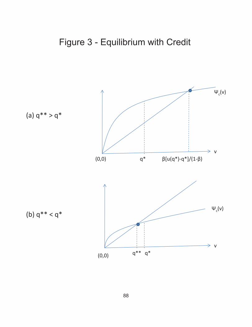
Figure 3 - Equilibrium with Credit

[u(q*) q*]/(1 )q*

c(v)

v(0,0)

c(v)

vq*q**(0,0)

(a) q** > q*

(b) q** < q*

Figure 3: Equilibrium with Credit

88

Figure 4 - Terms of Credit

89

w

R (w)

R

*w (w )*w

Figure 5 - Lender’s Cost Function

90

w [w (k)]*w[w (k )]*ww (k) w (k )* *

k < k