Georgia State University Georgia State University

ScholarWorks @ Georgia State University ScholarWorks @ Georgia State University

Economics Dissertations

August 2009

Essays on Interarea Wage Determination Essays on Interarea Wage Determination

John V. Winters

Follow this and additional works at: https://scholarworks.gsu.edu/econ_diss

Part of the Economics Commons

Recommended Citation Recommended Citation Winters, John V., "Essays on Interarea Wage Determination." Dissertation, Georgia State University, 2009. https://scholarworks.gsu.edu/econ_diss/1

This Dissertation is brought to you for free and open access by ScholarWorks @ Georgia State University. It has been accepted for inclusion in Economics Dissertations by an authorized administrator of ScholarWorks @ Georgia State University. For more information, please contact scholarworks@gsu.edu.

PERMISSION TO BORROW In presenting this dissertation as a partial fulfillment of the requirements for an advanced degree from Georgia State University, I agree that the Library of the University shall make it available for inspection and circulation in accordance with its regulations governing materials of this type. I agree that permission to quote from, to copy from, or to publish this dissertation may be granted by the author or, in his or her absence, the professor under whose direction it was written or, in his or her absence, by the Dean of the Andrew Young School of Policy Studies. Such quoting, copying, or publishing must be solely for scholarly purposes and must not involve potential financial gain. It is understood that any copying from or publication of this dissertation which involves potential gain will not be allowed without written permission of the author. ____________________________________ Signature of the Author

NOTICE TO BORROWERS All dissertations deposited in the Georgia State University Library must be used only in accordance with the stipulations prescribed by the author in the preceding statement. The author of this dissertation is: John V. Winters 252 Turnstone Road Stockbridge, GA 30281 The director of this dissertation is: Barry T. Hirsch Department of Economics Andrew Young School of Policy Studies Georgia State University P.O. Box 3992 Atlanta, Georgia 30302-3992 Users of this dissertation not regularly enrolled as students at Georgia State University are required to attest acceptance of the preceding stipulations by signing below. Libraries borrowing this dissertation for the use of their patrons are required to see that each user records here the information requested. Type of use Name of User Address Date (Examination only or copying)

ESSAYS ON INTERAREA WAGE DETERMINATION

BY

JOHN V. WINTERS        

A Dissertation Submitted in Partial Fulfillment of the Requirements for the Degree

of Doctor of Philosophy

in the Andrew Young School of Policy Studies

of Georgia State University

GEORGIA STATE UNIVERSITY 2009

Copyright by John Virgil Winters

2009

ACCEPTANCE This dissertation was prepared under the direction of the candidate’s Dissertation Committee. It has been approved and accepted by all members of that committee, and it has been accepted in partial fulfillment of the requirements for the degree of Doctor of Philosophy in Economics in the Andrew Young School of Policy Studies of Georgia State University. Dissertation Chair: Barry T. Hirsch Committee: Douglas J. Krupka David L. Sjoquist Mary Beth Walker Electronic Version Approved: W. Bartley Hildreth, Dean Andrew Young School of Policy Studies Georgia State University August 2009

iv  

ACKNOWLEDGEMENTS

This dissertation would not have been possible without the help, advice, and support of

many people. I would first like to thank my wife, Amanda, who always believed in me even

when I was close to doubting myself. Her love and support give me strength and have helped me

become a better man in all aspects of life. I would also like to thank the rest of my family for

their support during this long process.

I would next like to thank my chair, Dr. Barry Hirsch. His comments, suggestions, and

guidance have been instrumental in writing this dissertation. Dr. Hirsch has been an exceptional

mentor and has contributed greatly to my growth as a scholar. I also thank my supervisor and

committee member, Dr. David Sjoquist. Dr. Sjoquist has been an excellent boss and committee

member, and I will be forever grateful for his advice and support. I am also deeply indebted to

Dr. Douglas Krupka and Dr. Mary Beth Walker for serving on my committee and providing

guidance.

I also am grateful to the students, faculty, and staff at the Andrew Young School of

Policy Studies. Pursuing a Ph.D. has been a formidable challenge, and my ability to make it

through is due in no small part to my friends and colleagues in the Andrew Young School. I take

with me not only the knowledge gained from the program, but also the fond memories and the

eternal friendships I have made during my time here.

v  

TABLE OF CONTENTS

Pages

ACKNOWLEDGEMENTS …………………………………………………………………….. iv

LIST OF TABLES ……………………………………………………………………………... vii

ABSTRACT …...……………………………………………………………………………… viii

ESSAY I: WAGES AND PRICES: ARE WORKERS FULLY COMPENSATED FOR COST

OF LIVING DIFFERENCES …………………………………………………………………… 1

1. Introduction …………………………………………………………………………… 1

2. Theoretical Considerations .……………………...…………………………………… 4

3. Empirical Considerations/Previous Literature …...…………………………………… 8

4. Data and Methods ………………………………...…………………………………. 14

5. Empirical Results: The Elasticity between Wages and the General Price Level ……. 23

6. The Elasticity between Wages and the General Price Level for Alternative Specifications …………………………………………………...……………………… 30 7. Empirical Results: The Elasticity between Wages and Housing and Non-Housing Prices …………………………………………………...…………………….………… 41 8. Implications for Estimating Implicit Prices of Amenities …………...……………… 46

9. Conclusion …………………………………………………………………………... 48

ESSAY II: TEACHER SALARIES AND TEACHER UNIONS: A SPATIAL ECONOMETRIC

APPROACH ……………………………………………………………………………...……. 50

1. Introduction ………………………………………………………………………….. 50

2. Theory and Previous Literature ……………………………………………………... 52

3. Empirical Model …………………………………………………………………….. 56

vi  

4. Data ………………………………………………………………………………….. 60

5. Results ……………………………………………………………………………….. 65

6. Conclusion …….…………………………………………………………………….. 82

APPENDIX ……………………………………………………………………………………. 84

REFERENCES ……………………………………………………………………………….... 94

VITA ...……………………………………………………………………………………...… 100

vii  

LIST OF TABLES

Table Page

(Essay I) Table 1: Summary Statistics for Price Indices, 2006 ………………………………… 20

(Essay I) Table 2: OLS Results for Three Price Indices ……..………………………………… 24

(Essay I) Table 3: 2SLS Results for the Baseline Index ……..………………………………… 26

(Essay I) Table 4: 2SLS Results for the Rent-Based Modified Index .………………………… 27

(Essay I) Table 5: 2SLS Results for the Value-Based Modified Index ...……………………… 29

(Essay I) Table 6: 2SLS Results for the Rent-Based Index under Alternative Specifications … 31

(Essay I) Table 7: 2SLS Results for the Rent-Based Index by Education Group ……………... 36

(Essay I) Table 8: 2SLS Results for the Rent-Based Index with Spatial Lag and Spatial Error 40

(Essay I) Table 9: Separating Housing Prices (Rents) and Non-housing Prices ..……………... 42

(Essay I) Table 10: Separating Housing Prices (Values) and Non-housing Prices .…………… 45

(Essay I) Table 11: Amenity Values by Census Division ……..………………………………. 47

(Essay I) Appendix Table A: Housing Characteristic Results for Log Rent Equation, 2006 … 84

(Essay I) Appendix Table B: Price Indices by City, 2006 ……..……………………………… 85

(Essay I) Appendix Table C: Variables and Data Sources ...……..…………………………… 90

(Essay I) Appendix Table D: Additional 2SLS Regression Results for Preferred Specification 91

(Essay II) Table 1: Summary Statistics and Data Sources …………………………………….. 61

(Essay II) Table 2: Log Salary Regressions for MA20 with Union Indicator Variables ……… 66

(Essay II) Table 3: Log Salary Regressions for BA0 with Union Indicator Variables ..………. 68

(Essay II) Table 4: Log Salary Regressions for MA20 with State Collective Bargaining Share 74

(Essay II) Table 5: Log Salary Regressions for BA0 with State Collective Bargaining Share 75

(Essay II) Table 6: Log Salary Regressions for MA20 with State Union Membership Density 78

(Essay II) Table 7: Log Salary Regressions for BA0 with State Union Membership Density … 80

viii  

ABSTRACT

ESSAYS ON INTERAREA WAGE DETERMINATION

By

JOHN V. WINTERS

AUGUST 2009

Committee Chair: Dr. Barry T. Hirsch

Major Department: Economics

This dissertation consists of two essays concerning the determination of wages across

areas. The first essay investigates the equilibrium relationship between wages and prices across

labor markets. Of central interest is the extent to which workers receive higher wages to

compensate for differences in the cost of living. According to the spatial equilibrium hypothesis,

the utility of homogenous workers should be equal across labor markets. This implies that

controlling for amenity differences across areas, the elasticity between wages and the general

price level across areas should equal one, at least under certain conditions. We test this

hypothesis and find that the predicted relationship holds when housing prices are measured by

rents and the general price level is instrumented to account for measurement error. When

housing prices are measured by housing values, however, the wage-price elasticity is

significantly less than one, even using instrumental variables. Rents reflect the price paid for

housing per unit of time and are arguably the superior measure. Thus, findings in this essay

provide support for the full compensation hypothesis. These findings also have important

implications for researchers estimating the implicit prices of amenities or ranking the quality of

life across areas.

The second essay uses a national level dataset and a spatial econometric framework to

examine the effects of teacher unions and other school district characteristics on teacher salaries.

ix  

The results confirm that salaries for both experienced and beginning teachers are positively

affected by salaries in nearby districts. Investigations of the determinants of teacher salaries that

ignore this spatial relationship are likely to be misspecified. We find that union activity

increases salaries for experienced teachers by as much as 16-21 percent but increases salaries for

beginning teachers by a considerably smaller amount. This result is consistent with predictions

from a median voter model.

  

1  

ESSAY I: WAGES AND PRICES: ARE WORKERS FULLY COMPENSATED FOR

COST OF LIVING DIFFERENCES

1. Introduction

A number of studies have shown that wages differ across labor markets even after control

for observable individual characteristics.1 Such wage dispersion across markets can in part be

attributed to differences in prices and amenities across areas. If a city has higher prices for goods

and services providing a given level of utility, workers will require higher wages to work there.2

Similarly, if a city has nicer amenities, all else the same, workers will be willing to accept lower

wages to work there. In order for a spatial equilibrium to occur, utility must be equal across

areas for workers with identical skills and preferences. In previous literature, this is sometimes

referred to as the competitive hypothesis or the law of one wage. Many studies have attempted

to test the competitive hypothesis (e.g., regional wage gap studies), but they are often hindered

by limited information on area prices and amenities.

Several studies interested in interarea wage differentials have used an interarea price

index to fully adjust wages for price differences by dividing nominal wages by the price index.3

Other studies have used fully adjusted wages to measure the implicit prices of amenities across

cities (e.g., Rosen 1979; Greenwood et al. 1991; Glaeser and Tobio 2008).4 DuMond, Hirsch, and

Macpherson (1999), however, suggest that full adjustment for prices may be inappropriate to

measure interarea wage differentials, say by region or city size. They instead advocate using a

partial adjustment whereby the log of the price index (and potentially higher order terms) is                                                             1 See Dickie and Gerking (1989) for an early review of the literature on interarea wage differentials in the United States. 2 In this paper, we often use the term city to refer to metropolitan areas. 3 See for example, Coelho and Ghali (1971, 1973), Bellante (1979), Gerking and Weirick (1983), Johnson (1983), Sahling and Smith (1983), Dickie and Gerking (1987), and Farber and Newman (1987). 4 See Gyourko, Kahn and Tracy (1999) for a review of the literature on amenity valuation and quality of life.

2  

  

included as an independent variable in a log wage equation. The coefficient on the log of the

price index can be interpreted as the wage-price elasticity. One hypothesis is that the elasticity

between wages and the general price level is equal to one. We refer to this as the full

compensation hypothesis. Researchers who fully adjust wages for prices implicitly assume that

the full compensation hypothesis holds, but few studies have explicitly tested the full

compensation hypothesis.

Two studies that have estimated the elasticity between wages and prices are Roback

(1988) and DuMond et al. (1999). Roback (1988) uses a now discontinued cost of living index

produced by the Bureau of Labor Statistics and estimates a wage-price elasticity of 0.97, both

with and without controls for amenities, which would seem to lend support for the full

compensation hypothesis. As discussed below, a reexamination of Roback (1988), however,

suggests that her measurement of prices is inappropriate and biases her estimates. DuMond et

al. (1999) use a price index based on the ACCRA Cost of Living Index and find a wage-price

elasticity of 0.46 controlling for amenities and 0.37 absent amenities. Thus, the magnitude of the

wage-price elasticity and validity of the full compensation hypothesis are still open questions.

This paper builds on earlier work by examining the equilibrium relationship between

wages and prices, controlling for amenities. We stress the word equilibrium because wages and

prices are simultaneously determined. While this paper does not provide evidence on the causal

effect of prices on wages or vice versa, much can be learned from examining the equilibrium

relationship between the two. Following Rosen (1979) and Roback (1982), we develop a model

that predicts that under certain conditions the elasticity between wages and the general price

level should equal one controlling for amenities. In other words, workers should be fully

compensated for differences in prices across cities. However, to the extent that the assumptions

3  

  

of the model do not hold, the elasticity between wages and the general price level may differ

from unity. The relationship between wages and prices is ultimately an empirical question.

We find that estimates of the wage-price elasticity are sensitive to whether housing prices

are measured by housing values or rental payments. Rents are the ideal measure of housing

prices, the price paid per unit of time for the use of housing, but in practice housing values are

often used to measure housing prices. The preferred specification measures housing prices by

rents. Measuring housing prices by rents and using Ordinary Least Squares, we estimate the

wage-price elasticity to equal 0.76, but OLS estimates may be downwardly biased due to

measurement error in the price index, especially the non-housing price component.

Instrumenting for the rent-based price index using rents for the previous year, the estimated

elasticity between wages and the general price level is nearly identical to one. Again, if rents are

the ideal measure of housing prices, this finding provides strong empirical support for the full

compensation hypothesis.

When housing prices are measured by housing values, the estimated elasticity between

wages and the general price level is never more than 0.5, even using instrumental variables. The

findings of this paper have important implications for researchers estimating the implicit prices

of amenities or ranking the quality of life across areas. First, when adjusting wages for prices,

housing prices should be measured by rents and not values. Second, it is shown that ignoring

differences in non-housing prices, as often done, biases estimates of the implicit prices of

amenities.

4  

  

2. Theoretical Considerations

This section develops a simple model of the equilibrium relationship between wages,

prices, and amenities across cities and regions following Rosen (1979) and Roback (1982).

Firms produce and according to constant returns to scale production functions using labor

( ), capital ( ), and land ( ) given locational differences in productivity due to amenities ( ):

, , ; . The marginal products of labor, capital, and land are all non-negative, but

increases in amenities can either increase or decrease productivity. The price of capital is

determined exogenously in the world market and normalized to equal one, while the prices of

labor ( ) and land ( ) are determined competitively in local markets. In equilibrium, firms

earn zero profits and the price of each good is equal to its unit cost of production ( ):

, ; , = 1, 2. (1)

Workers maximize utility subject to a budget constraint, where utility is a function of

goods and and location-specific amenities: , ; . Workers are mobile across

cities and regions, and in equilibrium utility for identical workers is equal across areas. The

indirect utility function can be represented as a function of wages and the prices of and

given amenities:

, , ; . (2)

Taking the total differential of both sides of (2), setting = 0, rearranging, and employing

Roy’s Identity yields a slight variant of the equation used by Roback to estimate the implicit

price of amenities (Eq. 5 in Roback, 1982):

.5 (3)

                                                            5 Alternatively, we could have defined the expenditure function and used Shephard’s Lemma to obtain an equivalent result as in Albouy (2008b). 

5  

  

However, instead of solving for the price of amenities ( ), the equation is solved for .

Dividing both sides of (3) by , converts the equation to logarithmic form:

ln / ln / ln / . (4)

Equation (4) says that controlling for amenities, a one percent increase in the price of

will require wages to increase by a percentage equal to the share of wages spent on in order

for utility to remain constant. The same is true for increases in the price of , and the result

easily generalizes to the case of more than two goods. In other words, the wage-price elasticity

for a good should be equal to the budget share of the good, assuming that non-wage income is

negligible. Furthermore, if total consumption expenditure is equal to wage income,

, then a one percent increase in the prices of all goods will require wages to

increase by one percent to maintain equal utility.

While this interpretation of equation (4) is valid for small changes in prices, it may be

less valid for large changes in prices as consumers respond to large price differences by altering

their consumption mix. However, if utility is Cobb-Douglas as assumed by Davis and Ortalo-

Magné (2008) and others, the elasticity between wages and the price of a good is equal to the

expenditure share of the good even for large changes in prices. To see this, let utility take the

Cobb-Doulas form: . Taking a monotonic transformation, the indirect

utility function can be written as: ln ln 1 ln ln , where is

the constant budget share for , 1 is the budget share for , and is a constant.

Holding utility constant across areas, ∂ln / ∂ln is equal to even for large changes in prices.

In other words, Cobb-Douglas utility suggests that the elasticity between wages and the price of

a good is equal to the good’s budget share even for large price changes. Similarly, Cobb-Doulas

6  

  

utility predicts that the elasticity between wages and the general price level should equal one.

Workers would, therefore, require full compensation for price differences across cities.

The full compensation hypothesis has considerable intuitive appeal. Suppose there are

two cities with equal bundles of consumer amenities, but one city has higher prices for goods and

services. If the general price level in the expensive city is 10 percent higher than in the less

expensive city, how much higher will wages have to be in the expensive city to keep workers

from leaving for the other city? Intuition seems to suggest that a worker would need 10 percent

higher wages to compensate for the 10 percent higher price level. In other words, workers would

require full compensation for price differences holding amenities constant.

Workers may not be fully compensated for price differences for a number of reasons. If

workers are highly immobile or do not have sufficiently good information on wages, prices, and

amenities in other cities, then migration may not arbitrage away interarea differences in wages,

prices, and amenities. In other words, barriers to migration may cause workers in some markets

to have higher utility levels than comparable workers in other markets. In reality though,

workers are often quite mobile across markets. Even if some workers are relatively immobile,

the movement of marginal migrants between labor markets may result in an equilibrium

relationship between wages and prices that yields equal utility across areas for all homogenous

workers.

The relationship between wages and prices may also differ from full compensation if

utility is considerably different from Cobb-Douglas and prices are very different across markets.

Thinking of and in the above model as housing and non-housing consumption, a high

degree of substitutability between housing and non-housing may cause the true elasticity

7  

  

between wages and the general price level to be less than one.6 As will be shown later, housing

prices are significantly more dispersed across areas than non-housing prices. If workers can

easily substitute away from housing consumption in places where it is relatively expensive, they

will not have to be fully compensated for differences in housing prices.7 As a result, a fixed

basket price index will overstate the true cost of living in expensive cities and cause the elasticity

between wages and the general price level to be less than one.

As hinted above, the wage-price elasticity also depends on the extent to which people

save. If consumption is less than wage income ( ), the true wage-price

elasticity should be less than one. Conversely, if consumption is greater than wage income, the

wage-price elasticity may be greater than one. Evidence from the 2005 Consumer Expenditure

Survey suggests that average consumer expenditures are indeed quite close to average after-tax

wage income. The ratio of average expenditures to average after-tax income in the 2005 CES is 0.94.

The CES is a relatively small sample and there could be some misreporting (e.g., of income), but the

available evidence indicates that assuming expenditures are equal to wage income may be a reasonable

first approximation.

There are, therefore, a number of reasons why the elasticity between wages and the

general price level may be less than one. Ultimately, the relationship between wages and prices

is an empirical question. We explore this relationship empirically in subsequent sections.

                                                            6 Cobb-Douglas utility implies an elasticity of substitution equal to one. The limited literature has not reached a consensus on the elasticity of substitution between housing and non-housing. Ogaki and Reinhart (1998) estimate the elasticity of substitution to be 1.17, but not statistically different from one at the 5% significance level. Piazessi, Schneider, and Tuzel (2007) find estimates of 0.77 and 1.24 depending on the time period considered, neither of which is statistically different from one. However, Benhabib, Rogerson, and Wright (1991) and McGrattan, Rogerson, and Wright (1997) estimate the elasticity of substitution to be 2.5 and 1.75, respectively. Davis and Ortalo-Magné (2008) do not explicitly estimate the elasticity of substitution, but do find that the expenditure share on housing is roughly constant over time and across metropolitan areas suggesting that the elasticity of substitution is close to one. 7 Consumers may also shift away from consumption of relatively expensive housing toward consumption of local amenities, especially since local residents can often consume natural amenities at very low marginal cost (e.g., climate and coastal location). 

8  

  

3. Empirical Considerations/Previous Literature

The theoretical model suggests that under certain conditions, the elasticity between

wages and a composite price index is approximately one. Based on the intuition behind this

result, a number of researchers interested in interarea wage differentials have fully adjusted

nominal earnings using an interarea price index and estimated log wage equations of the form:

ln / , (5)

where is the wage for person in city , is the price level in city , is a vector of

personal characteristics, is the corresponding coefficient vector, and is an error term with

mean equal to zero. Along these lines, Johnson (1983) obtains the seemingly surprising result

that fully adjusted wages were more dispersed across cities than were nominal wages, at least for

men.8 DuMond et al. (1999), however, argue that full adjustment may be inappropriate. Instead,

they advocate using a partial adjustment where the dependent variable is the log of the nominal

wage and the log of the price index is included as an independent variable on the right hand side:

ln ln . (6)

Doing so, they find wage dispersion to be considerably lower across markets than with either

nominal or fully-adjusted wages.9

Theory and empirics also suggest that wages are affected by attributes that make a city a

more or less pleasant place to live. Therefore, (5) and (6) can also be modified to include city-

specific amenity levels and a corresponding coefficient vector. The parameter in (6) can be

interpreted as the interarea wage-price elasticity. If = 1, (5) and (6) are equivalent. However,

if is not equal to one, (5) may be misspecified. Thus the value of is of considerable interest.

                                                            8 Johnson (1983) uses a pooled cross-section of 34 cities from the May Current Population Survey for 1973-1976 with price data from the BLS for an intermediate standard of living for 1974. 9 DuMond et al. (1999) use a pooled cross-section of 185 cities from the 1985-1995 CPS Outgoing Rotation Group files with price data from the ACCRA Cost of Living Index from the same period.

9  

  

Roback (1988) estimates equation (6) both with and without amenities and produces

estimates of equal to 0.97 for both specifications. DuMond et al. (1999), however, estimate a

point estimate for of 0.46 with amenities and 0.37 without amenities with standard errors small

enough in both cases to easily reject the hypothesis that = 1. There are a number of differences

between the two studies, such as the time period considered, the number of cities considered and

the amenities included. However, the most important difference is likely the price indices used

and the way they are used. Roback uses a now discontinued price index produced by the Bureau

of Labor Statistics from the Handbook of Labor Statistics, and DuMond et al. use a price index

based on the ACCRA Cost of Living Index. Measurement error may be more significant in the

ACCRA price index, and this may explain some of the difference between the estimates of

Roback (1988) and DuMond et al. (1999). DuMond et al. reestimate their results using the BLS

Urban Family Budget and Comparative Indexes for Selected Urban Areas updated from its 1981

value (the last year the BLS produced the index) using the city-specific CPI for a limited number

of cities and find that the estimate of without amenities increases to 0.526. This price index is

much closer to the index used by Roback, but the coefficient estimate it yields is still much less

than one.

Closer examination of the two studies reveals a more subtle distinction in the way the

price indices are used. DuMond et al. (1999) use the same price index for all workers within a

given city. In Roback (1988), on the other hand, the price variable used consists of “low,

medium, and high standard of living budgets assigned based on individual family income and

number of dependents” (p.41). In other words, Roback assigns persons within a given city a

different price value based on their income. Presumably, her intent is to assign to each

individual the most relevant price for their particular consumption bundle. This approach creates

10  

  

intra-city variation in prices, and a problem arises if the intra-city variation in prices is spuriously

correlated with intra-city differences in wages. In such a case, the coefficient on the price

variable in the log equation will be biased. In other words, if the average price index value

across cities is greater for the high standard of living price index than for the intermediate index

and higher for the intermediate index than for the low index, then the price index is on average

increasing with income within cities. Indeed, a separate analysis suggests that this is the case for

the price information used by Roback. As a result, regressing log wages on a log price variable

constructed as such, the coefficient picks up a within-city effect in addition to the cross-city

effect. There may very well be differences in the relative cost of acquiring different standards of

living within a city, but accounting for this by introducing intra-city variation in the price index

that is explicitly tied to the observed wage is inappropriate. The principal focus should be on

cross-city and not within-city effects.

A further problem with Roback’s (1988) price variable is that she uses the actual budget

dollar amounts instead of price index values. The budgets formerly produced by the BLS are

based on what it would cost a family of four in a given city to obtain a given standard of living.

The BLS computes the budgets ( ) for each standard of living ( ) in each city ( ) by

multiplying local prices ( ) by a basket of goods ( ) for each standard of living. The basket

is also allowed to vary across cities within a standard of living, but is intended to maintain a

given standard of living across cities. Ignoring temporarily that the basket varies across cities,

recognize that . Regressing ln on ln( ) is clearly not the same as regressing

ln on ln because is increasing with income. If one were to use the same budget,

, (e.g., the intermediate standard of living budget) for all workers within a given city

and hence have no intra-city variation in budgets, then there would be no problem because taking

11  

  

logs causes ln to drop into the constant term. Using budgets instead of price index values and

allowing the budgets to vary across types of workers within cities means that the “price” variable

is severely confounded by intra-city variations in consumption. In other words, the estimates are

biased by the fact that workers within a city who have higher wages also have higher standards

of living and are assigned a higher consumption basket.

In work not shown, we attempt to replicate Roback’s (1988) empirical work and test the

sensitivity of the results to alternative measurement of prices. The results suggest that Roback’s

estimates are biased by using budgets rather than index values and allowing the budgets to vary

across workers within a given city. We first estimate by assigning all workers in a given city

the same index (or, equivalently, a common budget). We find wage-price elasticity estimates

without controls for amenities of 0.70, 0.56, and 0.45 using the low, intermediate, and high

standard of living price indices. We next assign budgets to workers based on standard of living

similar to Roback (1988). To do this, we assume that workers in the upper third of the within-

city income distribution have a high standard of living, workers in the middle third have an

intermediate standard of living, and workers in the lower third have a low standard of living.

Measuring prices in this manner, we find a wage-price elasticity of 1.00, again absent amenities.

This coefficient is very close to Roback’s estimate of 0.97, especially considering the replication

of how she assigns budgets is not exact. This estimate is likely biased, though, because budgets

are allowed to vary within cities, and hence the estimate largely reflects intra-city differences in

consumption. Alternatively, one can allow the price level to vary across standards of living, but

include standard of living dummies, so that identification comes only from inter-city variation in

12  

  

prices. Such estimation yields a wage-price elasticity of 0.46.10 These results are quite

interesting. When identification comes only from variation in prices across cities, the estimated

wage-price elasticity ranges from 0.45 to 0.70, depending on how prices are assigned. When we

allow identification from intra-city variation in assigned budgets, however, we get a coefficient

equal to one. Thus, it appears that Roback’s (1988) estimates are in error. However, the

replication of Roback (1988) here does not include amenities and does not account for

measurement error in the price index. In subsequent sections of this paper, we estimate the

wage-price elasticity using more recent data controlling for amenities and using instrumental

variables to account for measurement error.

Henderson (1982) also estimates a variant of equation (6) where he includes the log of

housing prices instead of a composite price index. The housing price measure used is the

estimated ownership cost for housing for an intermediate budget in the BLS Urban Family

Budget Data for Autumn 1977. Other studies have included housing prices in wage equations as

well, often as a control variable when the main investigation is something else, but Henderson is

one of the few to include housing prices along with amenities in an analysis of interarea wage

differentials. Henderson is also one of the few studies in this area to look at after-tax earnings

instead of pre-tax earnings. He finds point estimates of 0.17 and 0.21 for the coefficient on log

housing prices in alternate specifications that vary in the amenities included. Henderson does

not incorporate non-housing prices in his regressions, however, and he measures housing prices

by ownership costs, though rents are likely preferable.

Two recent working papers by Albouy (2008b) and Davis and Ortalo-Magné (2008) are

also interested in the relationship between wages and prices. Albouy (2008b) attempts to

                                                            10Similarly, including standard of living dummies and allowing the wage-price elasticity to vary by standard of living yields price coefficients of 0.59, 0.52, and 0.40 for the low, intermediate, and high standard of living groups, though the coefficients are not statistically different from each other at conventional levels.

13  

  

construct improved quality of life rankings for cities by among other things incorporating non-

housing prices and federal income taxes into the rankings. His main finding is that improved

quality of life estimates rank large cities more favorably than has been the case using previous

methods. He also computes city fixed effects for log housing prices and log wages and regresses

the log housing prices on log wages and amenities. The regression yields a coefficient of 1.41.

Based on his chosen parameters (for the budget shares of housing and non-housing, etc.), this

suggests that his model quite accurately predicts the relationship between housing prices and

wages across cities. The empirical work in the current paper differs from that in Albouy

(2008b) in at least two important ways. First, Albouy uses combined data on housing values and

rents to measure housing prices. The preferred estimates, however, in this paper measure

housing prices solely by rents. As shown later, the results in this paper are significantly affected

by measuring housing prices by values instead of rents. A second difference between the current

paper and Albouy (2008b) is that we estimate a wage-price elasticity, while he estimates a price-

wage elasticity. In theory, the two should be multiplicative inverses, ceteris paribus, but in

practice the two estimates differ in the treatment of non-housing prices. Albouy does not

explicitly control for non-housing prices, but instead infers non-housing prices from housing

prices.

Davis and Ortalo-Magné (2008) develop a model of the equilibrium relationship between

wages and prices across cities that assumes a Cobb-Douglas utility function and therefore that

the expenditure share for housing is constant across cities. They test their model by predicting

city-specific rental values as a function of wages and comparing predicted rents to observed

rents, where quality is held constant for both housing and labor. Davis and Ortalo-Magné predict

rents for city as a function of wages in the city according to the formula, / / ,

14  

  

where and are the mean values of rents and household wage income across cities, is

household wage income in city fully adjusted for the price of non-housing goods, and is the

constant expenditure share of housing, which Davis and Ortalo-Magné set equal to 0.24. They

find that observed rents are under-dispersed compared to what is predicted by their model, i.e.,

rents are too low in many high wage areas and too high in many low wage areas. Davis and

Ortalo-Magné concede that the omission of amenities from their analysis may adversely affect

their results. Measurement error in may also partially explain their findings.11

4. Data and Methods

In the empirical section of this paper, we begin by estimating a variant of equation (6)

that includes amenities ( ):

ln ln . (7)

We use earnings and individual characteristics data from the 2006 Current Population Survey

Outgoing Rotation Group (CPS-ORG) files merged with data on prices and amenities from

several sources.12 The sample used consists of all employed wage and salary workers ages 18-61

(inclusive), who are not full-time students. We also exclude all persons with imputed earnings to

avoid imputation bias, which would bias toward zero (Hirsch and Schumacher 2004; Bollinger

and Hirsch 2006).13 The dependent variable is the log of the hourly wage (ln ). We use the

reported hourly wage for workers who are paid by the hour and do not receive tips, commissions,

or overtime. For workers who are not paid by the hour or who receive tips, commissions or

                                                            11 This is conceptually similar to measurement error biasing the coefficient on wages in a rent regression toward zero. 12 Prices and amenities are measured at the city level, where a city is defined as a Core Based Statistical Area or a Combined Statistical Area. 13 Imputation bias would likely result because imputed earners are often assigned wages of workers in different metropolitan areas or even different regions.

15  

  

overtime, the hourly wage is computed by dividing usual weekly earnings by the usual number

of hours worked per week.

The preferred estimates adjust wages for federal income taxes, but we also estimate

equation (7) using pre-tax wages for the sake of comparison. As discussed by Henderson (1982)

and Albouy (2008a,b), the progressivity of the federal income tax system causes workers in high

wage areas to pay a higher percentage of their income in federal income taxes than workers in

relatively low wages areas. The marginal benefit, however, to an individual worker of her

federal income tax contributions is zero because workers consume the same level of federal

public services regardless of their federal tax payments. In other words, while workers pay

higher federal income taxes in high wage areas, they do not receive higher federal benefits.

Consequently, when choosing among cities, workers are concerned with the wages they would

earn net of federal taxes in each city instead of gross wages.

The present study does not adjust wages for social security contributions or state income

tax payments. It would be relatively straightforward to estimate social security contributions for

individual workers, but estimating the benefits to workers of their contributions would be more

difficult. We could also estimate state income tax payments for workers, but adjusting wages for

state income taxes is inappropriate unless we also adjust wages for other state and local taxes

because states differ in their reliance on income taxes. Even if we could compute the total

burden of all state and local taxes to each worker, we would still need to account for the benefits

from state and local expenditures that each worker receives. Given the complexities involved

with estimating the net fiscal incidence of social security payments and state taxes, we make no

adjustment for them in the dependent variable.14 Because the dependent variable in this study is

the log of the hourly wage, the analysis is only affected by social security payments and state                                                             14 Hence, use of the term after-tax wages implies wages net of federal income taxes only.

16  

  

taxes to the extent that their net fiscal incidence is not proportional to wages for homogenous

workers in different areas.15 However, to the extent that the total net burden of social security

and state and local taxes and expenditures for homogenous workers is higher (lower) in high

wage areas, regression estimates of that only account for federal income taxes may overstate

(understate) the true value of .

Federal income tax liabilities are not reported in the CPS-ORG files, but are instead

estimated using the federal tax schedule and based on several assumptions. We assume that all

married couples file jointly and receive two personal exemptions and non-married persons have a

filing status of single and receive one personal exemption. Itemized deductions are assumed to

equal 20 percent of annual earnings, where annual earnings are equal to usual weekly earnings

times 48.3 (the average number of weeks worked for workers in the March CPS). Taxpayers

take the standard deduction if it is more than their itemized deductions. Deductions and

exemptions are subtracted from annual earnings to estimate taxable income. Tax schedules are

then used to compute federal tax liabilities. We next compute the average tax rate for each

taxpayer ( ), and then multiply the hourly wage by one minus the average tax rate to compute

after-tax hourly wages ( 1 ).

All regressions include a number of individual characteristic variables intended to make

workers roughly similar across cities. The individual characteristics included are eleven dummy

variables for highest level of education received, a quartic specification for experience, and

dummy variables for mutually exclusive race/ethnicity categories (Black, Asian, Hispanic, and

other), female, married, employed part-time, enrolled part-time in school (measured for workers

                                                            15 To illustrate, suppose we have an equal rate tax ( ) on wages ( ) in all areas. Wages net of the tax are (1- ). Because the dependent variable is in logs, note that ln (1- )) = ln + ln(1- )). Because τ is a constant, regression results will be equivalent (except for the constant term in the regression) regardless of whether the dependent variable is the log of pre-tax wages (ln ) or the log of after-tax wages (ln (1- ))).

17  

  

under 25), union member, naturalized citizen, and non-citizen. Additionally, we include nine

occupation dummies, eleven industry dummies, and three dummies for whether the worker is a

federal, state, or local government employee. We also include 11 month-in-sample dummies.

The baseline price index is constructed using the ACCRA Cost of Living Index for 2006.

The ACCRA index is produced quarterly based on prices collected by local chambers of

commerce for a basket of 57 goods and services meant to be representative of actual consumer

expenditures.16 The prices of the 57 goods and services are then weighted (based somewhat on

CES expenditure data) to form a composite price index and six sub-indices for housing,

groceries, utilities, transportation, healthcare, and miscellaneous goods and services. However,

the baseline price index based solely on ACCRA data may not accurately measure intercity

variation in prices. One prominent reason is that ACCRA measures housing prices as a weighted

average of the price of two goods: apartment rent and homeowner principal and interest, with

homeowner costs being given a much greater weight (.82) than apartment rent (.18). Housing

rents measure the price paid per unit of time for the use of housing, and are therefore the ideal

measure of housing prices.17 Homeowner costs may be an inappropriate measure of the user cost

of housing because they are based on housing values. Homeownership involves both a

consumption decision and an investment decision, and the value of a house is equal to the

expected net present value of the income stream it generates. If expected future growth in rents

differs across cities and over time, then so will the ratios of rents to housing values. Empirical

evidence suggests that this is indeed the case (Clark 1995; Davis, Lehnert and Martin 2008).

                                                            16 While many of the goods in the index might be thought of as traded goods, the law of one price does not strictly hold because most goods are sold at retail. Retailing in San Francisco is more expensive than retailing in Topeka, KS because of higher commercial land rents and higher wages needed to compensate for higher housing rents (and subsequently higher non-housing costs). The spread of online shopping is likely to have important effects in pushing homogenous goods towards a single price, but this is not accounted for under current ACCRA methods. 17 For this reason, the Consumer Price Index produced by the BLS measures housing prices solely by rents.

18  

  

Housing values may even be subject to bubbles based on irrational speculation about the growth

in future benefits (Case and Schiller 2003). Therefore, measuring housing prices using house

values is likely to be inappropriate because house values are not based solely on the present user

cost of housing. This may be especially true for recent years given the relatively large increase

in housing values, especially in several metropolitan areas with a relatively inelastic supply of

housing (Glaeser, Gyourko and Saiz 2008).

Additional difficulties arise with the ACCRA index because prices are not reported for all

areas in each year. This has two drawbacks. First, ACCRA often contains no information on

prices for a given city, and hence we must exclude the city from the analysis. This limits the

analysis to 167 cities, though the cities that remain account for 68 percent of workers in the CPS.

A second problem is that prices are reported at the sub-metropolitan level and must be

aggregated to produce city-level averages using population weights, yet not all areas within a

metropolitan area are necessarily included. To the extent that sub-metropolitan areas for which

prices are reported are not representative of areas in the same city for which prices are not

reported, the average price level in the city will be measured with error. For a further discussion

of issues associated with using the ACCRA index to measure interarea price differences, see

Koo, Phillips, and Sigalla (2000).

To address the potential problems that result from using ACCRA data to measure

housing prices, we also compute a modified price index that measures housing prices solely by

rental costs from the 2006 American Community Survey (ACS).18 To do this, we use microdata

available from the Integrated Public Use Microdata Series (IPUMS) produced and distributed by

Ruggles et al. (2008) to estimate quality-adjusted average gross rents for each city in the

                                                            18 The ACCRA Cost of Living Index also reports average rents for an area, but for a number of reasons quality-adjusted rents from the ACS are likely preferable to rents from the ACCRA index.

19  

  

sample.19 The first step is to regress log gross rents, , for each housing unit on a vector of

housing characteristics, , and a vector of city-specific fixed effects, :

ln Γ . (8)

The housing characteristics included are dummy variables for the number of bedrooms, the total

number of rooms, the age of the structure, the number of units in the building, modern plumbing,

modern kitchen facilities, and lot size for single-family homes. The results for housing

characteristics from this estimation are generally as expected and are reported in Appendix Table

A. We then use the estimated parameters to predict average gross rents for each city holding the

housing characteristics constant at their mean level for the entire sample.20 We then divide the

quality-adjusted average gross rents for each city by the mean across cities and multiply by 100

to create a housing price index based on quality-adjusted gross rents. We then compute a

modified composite price index by taking a weighted average of the rent-based housing price

index and non-housing prices from ACCRA, where housing prices are given a weight of 0.29

and non-housing prices are a given a weight of 0.71.21 Weights are chosen based on calculations

from the 2005 Consumer Expenditure Survey suggesting that housing (based on gross rents)

represents 29 percent of average consumption expenditures.22

                                                            19 Gross rents include rents as well as basic utilities (water, electricity, and gas) and home heating fuels (wood, kerosene, oil, coal, etc.). These utilities are often included in rental payments for some renters, but not for others. Therefore, gross rents are more comparable across households because they include utilities and fuels for all renter households. 20 If, however, there are unobserved aspects of housing quality that are correlated with wages in a city, the estimated wage-price elasticity may be upwardly biased. 21 For these purposes, non-housing prices are computed as a weighted average of ACCRA sub-indices for groceries (0.13), transportation (0.25), healthcare (0.06), and miscellaneous goods and services (0.56). Note, that this excludes utilities in addition to housing because utilities are largely already included in gross rents. 22 Note that this expenditure share for housing differs from official reports of the CES expenditure share for both “Housing” and “Shelter.” The housing share based on gross rents used herein includes certain utilities but excludes others and also excludes expenditures for household operations, housekeeping, and household furnishings. The housing share of 0.29 also differs from the official CES tabulations in that homeowner housing expenditures are measured by implicit rents and not by out-of-pocket expenses such as mortgage interest.

20  

  

For the sake of comparison, we also compute a modified price index that measures

housing prices by quality-adjusted housing values from the 2006 ACS computed in a manner

similar to quality-adjusted gross rents. For this second modified price index, housing prices are

given a weight of 0.23 because values do not include utilities and non-housing prices (now

including utilities) are given a weight of 0.77.

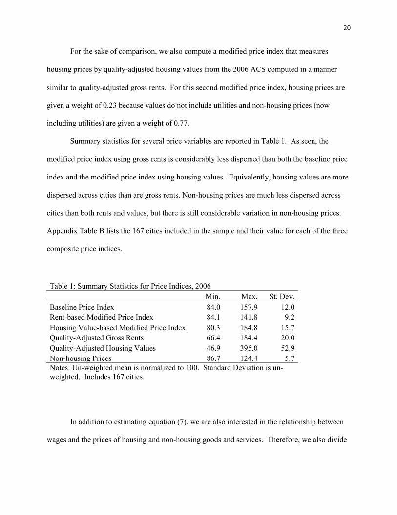
Summary statistics for several price variables are reported in Table 1. As seen, the

modified price index using gross rents is considerably less dispersed than both the baseline price

index and the modified price index using housing values. Equivalently, housing values are more

dispersed across cities than are gross rents. Non-housing prices are much less dispersed across

cities than both rents and values, but there is still considerable variation in non-housing prices.

Appendix Table B lists the 167 cities included in the sample and their value for each of the three

composite price indices.

Table 1: Summary Statistics for Price Indices, 2006 Min. Max. St. Dev. Baseline Price Index 84.0 157.9 12.0 Rent-based Modified Price Index 84.1 141.8 9.2 Housing Value-based Modified Price Index 80.3 184.8 15.7 Quality-Adjusted Gross Rents 66.4 184.4 20.0 Quality-Adjusted Housing Values 46.9 395.0 52.9 Non-housing Prices 86.7 124.4 5.7 Notes: Un-weighted mean is normalized to 100. Standard Deviation is un-weighted. Includes 167 cities.

In addition to estimating equation (7), we are also interested in the relationship between

wages and the prices of housing and non-housing goods and services. Therefore, we also divide

21  

  

the price index into housing prices, , and non-housing prices, , and include them in

logarithmic form in the log wage equation separately:

ln ln ln . (9)

Examining housing prices separately from non-housing prices is interesting for several reasons.

For one, it allows us to test if the prediction of equation (4) holds for housing and non-housing

prices separately. Additionally, a large literature in urban and regional economics following

Roback (1982) ranks the quality of life across cities using implicit prices of amenities computed

as the sum of compensating differentials in housing and labor markets, / / . Few

of these studies incorporate non-housing prices (Gabriel et al. 2003; Shapiro 2006; Albouy

2008b are recent exceptions). The justification for this exclusion is often that non-housing prices

are relatively unimportant (Beeson and Eberts 1989). The non-trivial variation in non-housing

prices illustrated in Table 1 combined with the large budget share for non-housing consumption,

however, suggests that non-housing prices may be quite important. The few papers that do

incorporate non-housing prices often do so in a less than ideal way.23 Separating housing and

non-housing prices allows us to examine the importance of each in explaining interarea wage

differentials.

Theory and previous empirical evidence predict that amenities also affect both wages and

local prices. Therefore, the regressions also include a number of different amenities from several

sources found to be important in previous literature.24 A list of variables and data sources is

included in Appendix Table C. Without including amenities, the estimated relationship between

                                                            23 For example, both Shapiro (2006) and Albouy (2008b) infer non-housing prices from housing prices by regressing non-housing prices on housing prices using the ACCRA Cost of Living Index. However, their approach ignores differences in non-housing prices across cities that are not correlated with housing prices. The analysis in this dissertation suggests that regressing non-housing prices on division dummies, city size dummies, and amenities in addition to housing prices does a much better job of predicting non-housing prices than housing prices alone. 24 Many of these are reported at the sub-metropolitan level and had to be aggregated to the CBSA/CSA level using populations as weights. 

22  

  

wages and prices could be biased.25 Data for several natural amenities are obtained from the

USDA Economic Research Service. These include the mean January temperature in degrees

Fahrenheit, mean July temperature, mean hours of January sunlight, mean July relative humidity,

the percent of land area covered by water, and five indicator variables for topography that range

from very flat to mountainous. The flattest land surface is the omitted reference group. Mean

annual inches of precipitation and snow are obtained from Cities Ranked and Rated, 2nd Edition.

Maps were consulted to create indicator variables for whether a city is located on the coast of the

Atlantic Ocean, Pacific Ocean or Gulf of Mexico. Data on violent crime and property crime per

capita were obtained from the Census Bureau’s USA Counties website.26 The mean commuting

time in minutes for workers in a city was computed using the 2006 ACS microdata. Two

measures of air pollution, ozone and particulate matter 2.5, were computed using the EPA

AirData database.27 The regressions also include eight census division dummies and six city

population size dummies to account for residual differences in amenities.28 The city size

dummies should also help control for differences in unobserved worker ability across cities.29

No specification of amenities is likely to fully capture differences in the quality of life across

cities, but the hope is that the variables used in this paper do a reasonably good job of controlling

for differences in the quality of life across cities.

                                                            25 For example, a pure consumption amenity is likely to drive up housing prices and drive down wages, which would bias the wage-price elasticity toward zero. 26 http://censtats.census.gov/usa/usa.shtml. 27 Pollution values were unavailable for several small cities and were imputed based on average values by Census division and city size. Particulate matter was imputed in this manner for 16 cities, and ozone was imputed for 23 cities. We tested the potential effect of this imputation by estimating the regressions without pollution variables and estimating the regressions with pollution variables but only for cities that had unimputed pollution levels. The main results of this paper do not appear to be affected by the imputation of pollution values for these small cities. 28 The seven city size categories are: 0-199,999; 200,000-299,999; 300,000-499,999; 500,000-999,999; 1,000,000-1,999,999; 2,000,000-4,999,999; and 5,000,000+. 29 Glaeser and Maré (2001), Yankow (2006), and Krupka (2008) all find that the nominal city size wage premium falls after controlling for individual fixed effects using panel data on workers, suggesting that large cities attract more able workers.

23  

  

5. Empirical Results: The Elasticity between Wages and the General Price Level

This section presents results of the elasticity between wages and the general price level

using the baseline price index, the price index modified using quality-adjusted gross rents, and

the price index modified using quality-adjusted house values. All regressions include the full list

of amenities, division dummies, city size dummies, and individual characteristics as explanatory

variables. The results for these variables were generally as expected. Full results for the

preferred specification are provided in Appendix Table D.30 We begin by estimating the

regressions using Ordinary Least Squares and then proceed to instrument for prices to account

for measurement error, which would bias the estimated coefficients toward zero. All of the price

index coefficients in this section are statistically different from zero at the 1% level using cluster

robust standard errors, but the more appropriate null hypothesis is whether or not they are

different from unity.31

Ordinary Least Squares

We first estimate the wage-price elasticity, , using the baseline price index via OLS.

This specification is comparable to that of DuMond et al. (1999), but the equation herein

contains many more amenities, more recent data, and uses after-tax wages as the dependent

variable.32 As seen in the first column of Table 2, this specification yields an estimate of of

0.314, and the coefficient is statistically different from one at the 1% level. According to this

estimate, a one percent increase in the general price level in a city is associated with a 0.31

percent increase in after-tax wages. This is also considerably lower than the previous estimate of

0.46 by DuMond et al. (1999). This may suggest that the sharp increase in housing values in

                                                            30 As discussed in more detail later, the preferred specification is to measure prices by the log of the rent-based price index and instrument using log gross rents from the previous year. 31 Unless otherwise noted, all standard errors in this paper are robust clustered by city. 32 A more subtle difference is that DuMond et al. (1999) include workers with imputed earnings, which likely biases their estimates toward zero.

24  

  

recent years causes the ACCRA index to be a worse measure of the cost of living in 2006 than it

was between 1985 and 1995, the time period considered by DuMond et al. (1999).

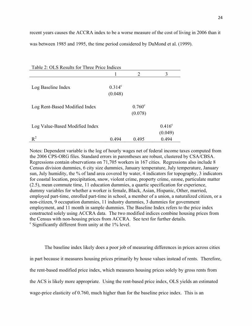
Table 2: OLS Results for Three Price Indices 1 2 3

Log Baseline Index 0.314c (0.048)

Log Rent-Based Modified Index 0.760c (0.078)

Log Value-Based Modified Index 0.416c (0.049)

R2 0.494 0.495 0.494 Notes: Dependent variable is the log of hourly wages net of federal income taxes computed from the 2006 CPS-ORG files. Standard errors in parentheses are robust, clustered by CSA/CBSA. Regressions contain observations on 71,705 workers in 167 cities. Regressions also include 8 Census division dummies, 6 city size dummies, January temperature, July temperature, January sun, July humidity, the % of land area covered by water, 4 indicators for topography, 3 indicators for coastal location, precipitation, snow, violent crime, property crime, ozone, particulate matter (2.5), mean commute time, 11 education dummies, a quartic specification for experience, dummy variables for whether a worker is female, Black, Asian, Hispanic, Other, married, employed part-time, enrolled part-time in school, a member of a union, a naturalized citizen, or a non-citizen, 9 occupation dummies, 11 industry dummies, 3 dummies for government employment, and 11 month in sample dummies. The Baseline Index refers to the price index constructed solely using ACCRA data. The two modified indices combine housing prices from the Census with non-housing prices from ACCRA. See text for further details. c Significantly different from unity at the 1% level.

The baseline index likely does a poor job of measuring differences in prices across cities

in part because it measures housing prices primarily by house values instead of rents. Therefore,

the rent-based modified price index, which measures housing prices solely by gross rents from

the ACS is likely more appropriate. Using the rent-based price index, OLS yields an estimated

wage-price elasticity of 0.760, much higher than for the baseline price index. This is an

25  

  

important result. It appears that the wage-price elasticity using the baseline price index is biased

toward zero in part because of how housing prices are measured. However, this estimate for the

rent-based index is still significantly less than one.

We also estimate using the housing value-based modified price index. Using OLS, the

estimated coefficient is 0.416 and is significantly less than one. Interestingly, the coefficient for

the value-based modified index is greater than that for the baseline index. This suggests that

measuring housing prices by values may not be the only source of measurement error in the

baseline index.33

Instrumental Variables

Even after measuring housing prices by quality-adjusted gross rents from the ACS, the

price index may still be measured with considerable error. Housing prices as measured are likely

subject to some degree of sampling error and non-housing prices measured in the ACCRA Cost

of Living Index may be subject to a number of sources of measurement error. Random

measurement error will bias the coefficient on the log price index toward zero, and including

variables that are highly correlated with the price index such as amenities, division dummies, and

city size dummies, may exacerbate measurement error bias. We next use instrumental variables

to account for measurement error in the price indices. We use as instruments the lagged housing

and non-housing components of the individual price indices. If measurement error is random,

then instrumenting for the price index using the previous year’s components should produce

consistent estimates of . If measurement error in the price index is serially correlated, however,

instrumenting using lagged prices will not produce consistent coefficient estimates. Tables 3, 4,

                                                            33 It may also be the case that housing values are measured with greater error than rents and this leads to greater measurement error bias for the value-based modified index than the rent-based index. Bucks and Pence (2006), however, report that homeowner reported housing values are fairly accurate.

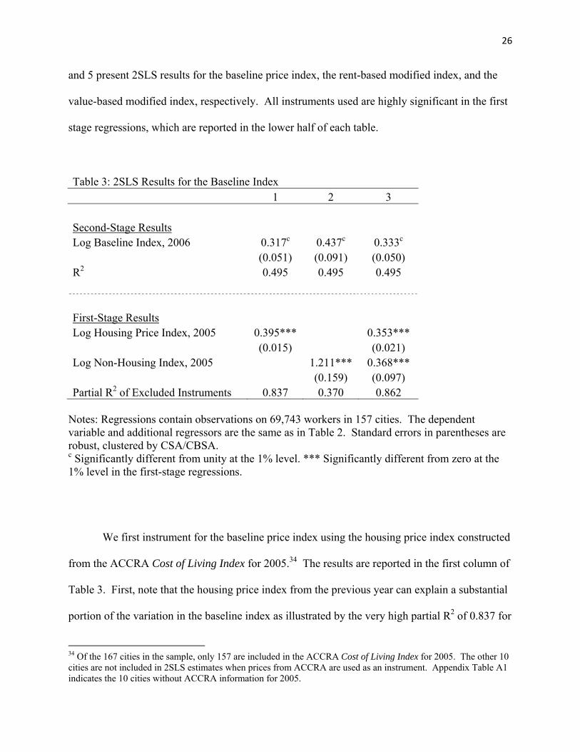
26  

  

and 5 present 2SLS results for the baseline price index, the rent-based modified index, and the

value-based modified index, respectively. All instruments used are highly significant in the first

stage regressions, which are reported in the lower half of each table.

Table 3: 2SLS Results for the Baseline Index 1 2 3

Second-Stage Results Log Baseline Index, 2006 0.317c 0.437c 0.333c

(0.051) (0.091) (0.050) R2 0.495 0.495 0.495

First-Stage Results Log Housing Price Index, 2005 0.395*** 0.353***

(0.015) (0.021) Log Non-Housing Index, 2005 1.211*** 0.368***

(0.159) (0.097) Partial R2 of Excluded Instruments 0.837 0.370 0.862

Notes: Regressions contain observations on 69,743 workers in 157 cities. The dependent variable and additional regressors are the same as in Table 2. Standard errors in parentheses are robust, clustered by CSA/CBSA. c Significantly different from unity at the 1% level. *** Significantly different from zero at the 1% level in the first-stage regressions.

We first instrument for the baseline price index using the housing price index constructed

from the ACCRA Cost of Living Index for 2005.34 The results are reported in the first column of

Table 3. First, note that the housing price index from the previous year can explain a substantial

portion of the variation in the baseline index as illustrated by the very high partial R2 of 0.837 for

                                                            34 Of the 167 cities in the sample, only 157 are included in the ACCRA Cost of Living Index for 2005. The other 10 cities are not included in 2SLS estimates when prices from ACCRA are used as an instrument. Appendix Table A1 indicates the 10 cities without ACCRA information for 2005.

27  

  

the first-stage regression. The coefficient of the log of the baseline price index in the log wage

equation, however, is virtually identical to the OLS result. We next instrument for the baseline

index using non-housing prices for the previous year. As seen, lagged non-housing prices

explain less of the variation in the baseline index (though still a considerable amount), but the

second-stage coefficient does increase somewhat to 0.437. In the third column of Table 3, we

include lagged housing and non-housing prices together as instruments yielding a coefficient of

0.333 in the second-stage regression. Thus regardless of the instrument(s) used, the estimated

elasticity between wages and prices is still considerably less than one using the baseline price

index.

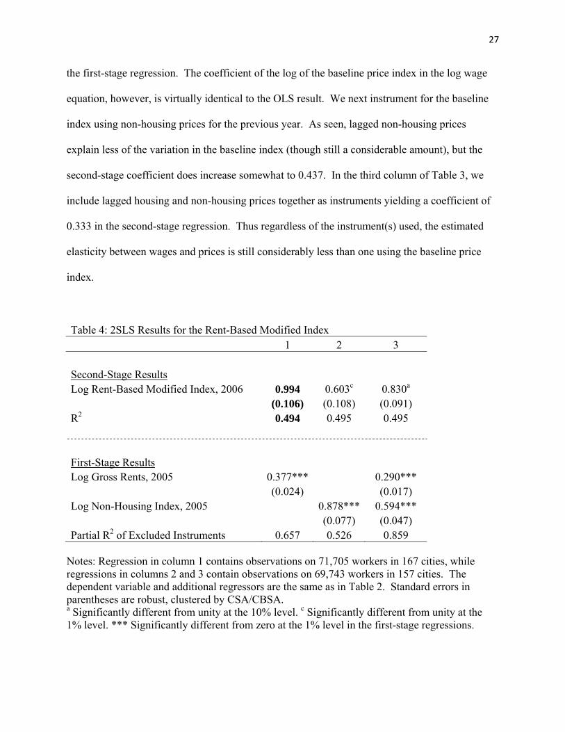
Table 4: 2SLS Results for the Rent-Based Modified Index 1 2 3

Second-Stage Results Log Rent-Based Modified Index, 2006 0.994 0.603c 0.830a

(0.106) (0.108) (0.091) R2 0.494 0.495 0.495

First-Stage Results Log Gross Rents, 2005 0.377*** 0.290***

(0.024) (0.017) Log Non-Housing Index, 2005 0.878*** 0.594***

(0.077) (0.047) Partial R2 of Excluded Instruments 0.657 0.526 0.859

Notes: Regression in column 1 contains observations on 71,705 workers in 167 cities, while regressions in columns 2 and 3 contain observations on 69,743 workers in 157 cities. The dependent variable and additional regressors are the same as in Table 2. Standard errors in parentheses are robust, clustered by CSA/CBSA. a Significantly different from unity at the 10% level. c Significantly different from unity at the 1% level. *** Significantly different from zero at the 1% level in the first-stage regressions.

28  

  

We next use 2SLS for the preferred measure of prices, the rent-based modified price

index. While the OLS coefficient estimate for the rent-based price index is much closer to unity

than the baseline index, it is still significantly less than one. If random measurement error is

driving the coefficient away from one, then instrumenting may produce consistent estimates. We

first instrument for the log of the rent-based modified price index using quality-adjusted log

gross rents from the previous year. As reported in the first column of Table 4, instrumenting in

this manner yields a coefficient estimate of 0.994 that is nearly identical to one. Therefore,

instrumenting for the rent-based price index using rents for the previous year provides empirical

support for the full compensation hypothesis. We next instrument for the rent-based modified

index using non-housing prices for the previous year. The 2SLS coefficient estimate in this case,

0.603, is considerably lower than that found using OLS. Finally, when we use both gross rents

and non-housing prices as instruments for the rent-based price index, we get a coefficient

estimate of 0.830 that is statistically different from unity at the 10% level.

Non-housing prices are constructed from the ACCRA Cost of Living Index and are likely

subject to considerable measurement error, some of which is likely persistent within cities over

time. If measurement error in non-housing prices is serially correlated, then instrumenting for

the general price level using non-housing prices will not yield consistent estimates of . The

divergence between the estimates in the first and second columns of Table 4 suggests that this is

indeed the case. Quality-adjusted gross rents are estimated from the ACS PUMS and may also

be subject to some measurement error such as due to sampling. However, the measurement error

in log gross rents is much more likely to be classical in nature. If the measurement error in the

lag of log gross rents is purely random and uncorrelated with measurement error in the rent-

based price index, then the 2SLS estimates in the first column of Table 4 are consistent. This

29  

  

seems quite plausible. If log gross rents are a valid instrument, over-identification in the

specification of the third column allows us to examine the validity of non-housing prices as an

instrument. Doing so, we get a Hansen J Statistic of 11.297, which allows us to reject non-

housing prices as a valid instrument at the 1% level. Thus the coefficient in the first column of

Table 4 is the preferred estimate of the elasticity between wages and the general price level.

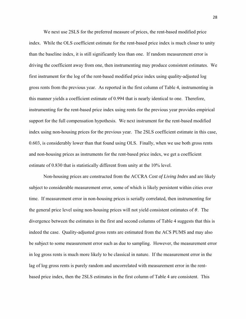
Table 5: 2SLS Results for the Value-Based Modified Index 1 2 3

Second-Stage Results Log Value-Based Modified Index, 2006 0.478c 0.395c 0.447c

(0.059) (0.071) (0.052) R2 0.494 0.495 0.495

First-Stage Results Log Housing Values, 2005 0.347*** 0.294***

(0.015) (0.017) Log Non-Housing Index, 2005 1.340*** 0.552***

(0.138) (0.077) Partial R2 of Excluded Instruments 0.835 0.481 0.899

Notes: Regression in column 1 contains observations on 71,705 workers in 167 cities, while regressions in columns 2 and 3 contain observations on 69,743 workers in 157 cities. The dependent variable and additional regressors are the same as in Table 2. Standard errors in parentheses are robust, clustered by CSA/CBSA. c Significantly different from unity at the 1% level. *** Significantly different from zero at the 1% level in the first-stage regressions.

For the sake of comparison, we also estimate the wage-price elasticity for the value-based

modified price index using 2SLS. The results are presented in Table 5. In all three columns, the

coefficient on the value-based price index is considerably less than one, again suggesting that

30  

  

measuring housing prices by housing values is inappropriate. Interestingly, though, the estimates

in the first and third columns are a little higher than the corresponding estimates for the baseline

index in Table 3, while the estimate in the second column that instruments for the general price

level using non-housing prices is lower than in Table 3.

A recap of the results in this section is warranted. Theory and intuition predict that the

elasticity between wages and the general price level should be close to one. When housing

prices are measured by homeowner values, the estimated elasticity between wages and the

general price level is never more than 0.5, even when we use instrumental variables to account

for measurement error. When housing prices are measured by rents, though, the estimated

elasticity between wages and the general price level increases considerably. Using OLS the

estimated wage-price elasticity is still less than one, but instrumenting for the log of the rent-

based modified price index using the log of quality-adjusted gross rents for the previous year, the

wage-price elasticity is equal to one for all practical purposes. This result supports the full

compensation hypothesis and has important implications for researchers estimating the implicit

prices of amenities. In the next section, we examine the sensitivity of to alternative

specifications.

6. The Elasticity between Wages and the General Price Level for Alternative Specifications

In this section, we briefly examine the sensitivity of the 2SLS wage-price elasticity

estimates using the rent-based price index to alternative specifications and samples. The results

prove to be quite robust. The first row of Table 6 reproduces estimates for the preferred

specification from the first column of Table 4 in which we instrument for the log of the rent-

based price index using log gross rents from the previous year. The remainder of Tables 6, 7,

31  

  

and 8 present results for alternative specifications and samples instrumenting for the log of the

rent-based priced index using log gross rents.

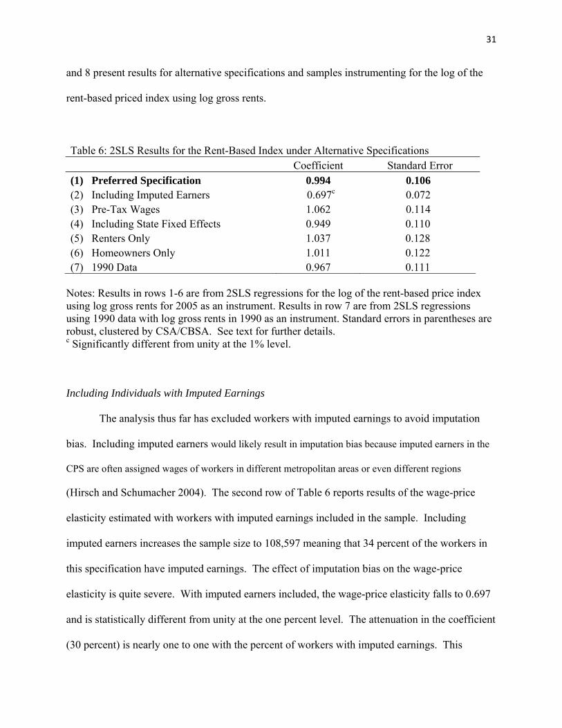
Table 6: 2SLS Results for the Rent-Based Index under Alternative Specifications Coefficient Standard Error (1) Preferred Specification 0.994 0.106 (2) Including Imputed Earners 0.697c 0.072 (3) Pre-Tax Wages 1.062 0.114 (4) Including State Fixed Effects 0.949 0.110 (5) Renters Only 1.037 0.128 (6) Homeowners Only 1.011 0.122 (7) 1990 Data 0.967 0.111

Notes: Results in rows 1-6 are from 2SLS regressions for the log of the rent-based price index using log gross rents for 2005 as an instrument. Results in row 7 are from 2SLS regressions using 1990 data with log gross rents in 1990 as an instrument. Standard errors in parentheses are robust, clustered by CSA/CBSA. See text for further details. c Significantly different from unity at the 1% level.

Including Individuals with Imputed Earnings

The analysis thus far has excluded workers with imputed earnings to avoid imputation

bias. Including imputed earners would likely result in imputation bias because imputed earners in the

CPS are often assigned wages of workers in different metropolitan areas or even different regions

(Hirsch and Schumacher 2004). The second row of Table 6 reports results of the wage-price

elasticity estimated with workers with imputed earnings included in the sample. Including

imputed earners increases the sample size to 108,597 meaning that 34 percent of the workers in

this specification have imputed earnings. The effect of imputation bias on the wage-price

elasticity is quite severe. With imputed earners included, the wage-price elasticity falls to 0.697

and is statistically different from unity at the one percent level. The attenuation in the coefficient

(30 percent) is nearly one to one with the percent of workers with imputed earnings. This

32  

  

reaffirms the initial decision to exclude workers with imputed earnings as suggested by recent

literature.

Pre-tax Wages

In the third row of Table 6, we estimate via 2SLS using pre-tax wages as the dependent

variable. As pointed out by Henderson (1982) and Albouy (2008a,b), the progressivity of the

federal income tax causes workers in cities with high nominal wages to pay a higher percentage

of their income in federal income taxes than workers in cities with lower nominal wages. For the

utility of homogenous workers to be constant across areas, pre-tax wages should be more

dispersed across areas than after-tax wages. In other words, workers in high wage areas must be

compensated for the higher federal income taxes they pay in addition to the compensation they

require for the higher cost of living or worse bundle of amenities. As such, the estimated wage-

price elasticity should be higher using pre-tax wages than using after-tax wages. The results in

row 3 suggest that this is likely the case. The estimate of increases to 1.062, but is not

statistically different from unity. We maintain, however, that it is after-tax wages that should

equalize across areas controlling for prices, amenities, and individual characteristics, so

measuring wages net of federal income tax provides a better test of the theory than measuring

wages before federal income tax.

State Fixed Effects

If wages should be measured net of federal income tax, we might also consider adjusting

wages for state and local income taxes. Income taxes, however, are only part of the story at the

states and local level. To adjust wages for state and local income taxes, we would also need to

incorporate information on other state and local taxes and state and local public spending. To

avoid the many complexities involved with adjusting wages for state and local taxes and

33  

  

expenditures, we adopt a different approach by examining the robustness of the results to

including state fixed effects. If ignoring state taxes and expenditures is biasing the previous

results, then we would expect that including state fixed effects would produce a very different

estimate of than the case in which we include census division fixed effects. As seen in row 4,

including state fixed effects reduces the coefficient estimate to 0.949, but it is not statistically

different from one. Therefore, the basic findings of this paper are robust to including state fixed

effects. The preferred specification, however, is to use census division dummies and not state

fixed effects because several states contain only one city in the sample. Including state fixed

effects means that is only estimated based on states that have more than one city in the sample.

Renters vs. Homeowners

One might also wonder if using a rent-based price index yields different estimates of

for renters and homeowners. In particular, one might be concerned that the rent-based price

index does not accurately measure the prices faced by homeowners and could cause estimates

for the two groups to diverge. Rows 5 and 6 of Table 6 estimate separately for renters and

homeowners. The coefficient estimate for renters is 1.037, and the estimate for homeowners is

1.011. Therefore, the coefficient estimates for renters and homeowners separately are slightly

higher than the pooled estimate, but neither estimate is statistically different from unity. The

coefficient estimates for renters and homeowners are also not statistically different from each

other. It appears that differences in prices across cities affect the wages of renters and

homeowners roughly the same.

An Earlier Period: 1990

To ensure that the results are not being driven by the particular year chosen, we next

reestimate the wage-price elasticity using 1990 data from the CPS, the ACCRA Cost of Living

34  

  

Index, Census microdata, and the various sources of information on amenities, constructing

prices and amenities as before.35 The 1990 sample contains 84,117 observations in 155 cities.

The preferred instrument would be to use log gross rents from the previous year, but

unfortunately the most recent prior year would be 1980. Instead of using housing prices from

such a distant earlier period, we use log gross rents from 1990. If measurement error in the log

of the rent-based price index is correlated with measurement error in log gross rents, coefficient

estimates from this procedure will be downwardly biased. However, because gross rents from

the Census are expected to be measured with relatively little error, downward bias due to

measurement error is likely to be minimal. Row 7 of Table 6 presents the wage-price elasticity

estimate using data for 1990. The estimate is 0.967 and not statistically different from unity.

Thus it appears that the finding of a wage-price elasticity of unity for the rent-based price index

is robust to this earlier period chosen.36

By Educational Attainment

We may also be concerned that using a single price index ignores differences in prices

within cities for different standards of living. Workers do not care about the average price level

in a city, but instead care about the prices of goods that they consume. If the relative cost of

living in a city varies significantly across different types of workers, estimating θ using a single

price index for all workers may be inappropriate. This concern motivated Roback (1988) to use

separate price indices for workers with different standards of living.

                                                            35 One subtle difference in the price index is that the shares of housing and non-housing goods in the rent-based price index are different than in 2006. While gross rents represented 29 percent of total household expenditures in the 2005 CES, the share was only 24 percent for the 1990 CES. Therefore, the 1990 rent-based price index gives housing prices based on Census microdata a weight of 0.24 and non-housing prices from ACCRA a weight of 0.76. 36 We also estimate the wage-price elasticity for 1990 using a value-based modified index similar to that used above. Using 2SLS with log housing values as an instrument, we find a wage-price elasticity for this price index of 0.579 that is statistically different from one. While this estimate is higher than the corresponding estimate of 0.478 in the first column of Table 5 and would likely be even higher in the absence of measurement error, it is still quite a bit less than unity. This again reaffirms the earlier finding that housing values are an inappropriate measure of the price of housing consumption.

35  

  

To explore the importance of price differences across standards of living, we form

separate rent-based price indices for four educational groups: high school dropouts, high school

graduates, persons with some college, and persons with a bachelor’s degree or higher. Non-

housing prices are taken to be the same for all four groups, but housing prices are allowed to

vary by income group in a similar method to that used by Moretti (2008). First, the rent

regression of equation (8) is estimated separately for each education group. The estimated

parameters are then used to predict quality-adjusted average gross rents for each city and

education group holding the housing characteristics constant at their mean level for the education

group. Quality-adjusted gross rents for each education level are then combined with non-

housing prices to form separate rent-based modified price indices for the four education groups

with non-housing prices given a weight of 0.71 and housing prices given a weight of 0.29 as

before.

Because there are now four different price indices, we estimate the wage-price elasticity

via equation (7) separately for each education group using their education-specific price index.

Before doing so, however, it is useful to first estimate the wage-price elasticity separately for

each education group using the rent-based index used above that does not vary by education. In

other words, we wish to see if the wage-price elasticity varies by education group using the same

rent-based price index for all education groups. To do so, we instrument for the log of the

general price level using log gross rents from the previous year. The results in the upper panel of

Table 7 suggest that the wage-price elasticity does indeed vary by education group and is

decreasing with education. DuMond et al. (1999) also find the wage-price elasticity to be

generally decreasing with education, though their estimates were less than unity for all four

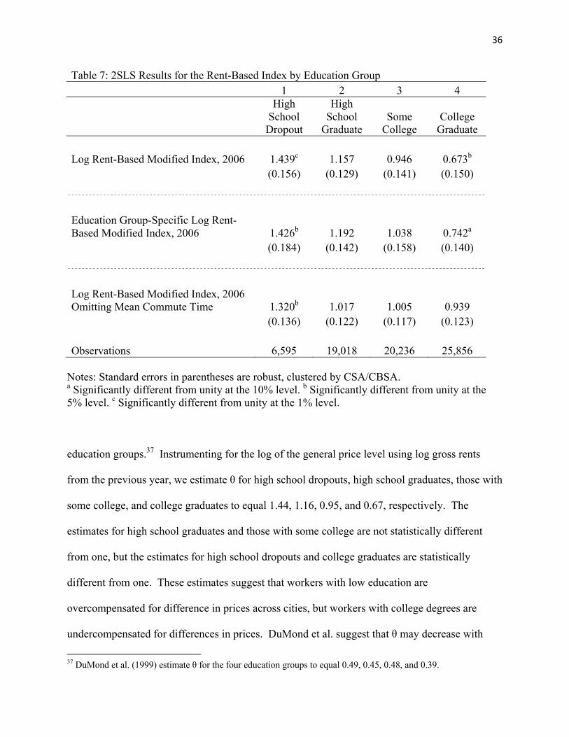
36  

  

Table 7: 2SLS Results for the Rent-Based Index by Education Group 1 2 3 4

High School

Dropout

High School

Graduate Some

College College

Graduate

Log Rent-Based Modified Index, 2006 1.439c 1.157 0.946 0.673b (0.156) (0.129) (0.141) (0.150)

Education Group-Specific Log Rent-Based Modified Index, 2006 1.426b 1.192 1.038 0.742a

(0.184) (0.142) (0.158) (0.140)

Log Rent-Based Modified Index, 2006 Omitting Mean Commute Time 1.320b 1.017 1.005 0.939

(0.136) (0.122) (0.117) (0.123)

Observations 6,595 19,018 20,236 25,856 Notes: Standard errors in parentheses are robust, clustered by CSA/CBSA. a Significantly different from unity at the 10% level. b Significantly different from unity at the 5% level. c Significantly different from unity at the 1% level.

education groups.37 Instrumenting for the log of the general price level using log gross rents

from the previous year, we estimate θ for high school dropouts, high school graduates, those with

some college, and college graduates to equal 1.44, 1.16, 0.95, and 0.67, respectively. The

estimates for high school graduates and those with some college are not statistically different

from one, but the estimates for high school dropouts and college graduates are statistically

different from one. These estimates suggest that workers with low education are

overcompensated for difference in prices across cities, but workers with college degrees are

undercompensated for differences in prices. DuMond et al. suggest that θ may decrease with

                                                            37 DuMond et al. (1999) estimate θ for the four education groups to equal 0.49, 0.45, 0.48, and 0.39.

37  

  

education because educated workers are better able to shift away from housing in areas where

housing is relatively expensive. Similarly, we might also expect θ to decrease with education if

housing is a more important share of consumption for less educated workers.38

It could also be the case that using average prices for all workers adversely affects the

estimates. Thus, using the education-specific price indices could yield estimates close to unity

for all groups. When we estimate equation (7) separately for each education group using the

education-specific price indices, however, the results are not significantly affected as seen in the

middle portion of Table 7. The estimates of θ for the four education groups are 1.43, 1.19, 1.04,

and 0.74. In other words, while there may be differences in the wage-price elasticity by

education group, differences in the price of housing by education group do not appear to be an

important part of the explanation.

The estimated wage-price elasticity may also differ across education groups because

coefficient estimates for other variables vary by education group. Examining the coefficient

estimates for the other variables, one sticks out as particularly troubling. According to the

estimates, mean commute time has a very different effect on the wages of workers in different

education groups. For the regressions in the upper portion of Table 7, the coefficients for mean

commute time are -0.52, -0.64, 0.27, and 1.12, though only the estimates for high school

graduates and college graduates are statistically different from zero.39 Our expectation is that

longer commutes in a city should be a disamenity and we expect commute time to have a

positive sign. However, collinearity between the price index and commute time may be

                                                            38 This would result because understating housing’s share of consumption would cause the composite price index to be under-dispersed. Under-dispersion in the price index would cause the estimated wage-price elasticity to be too large. 39 The coefficient for mean commute time in the preferred specification in the first column of Table 4 is 0.12 and not statistically different from zero.

38  

  

influencing the estimates of both. As the coefficient for commute time increases, the coefficient

for the price index decreases and vice versa.

Therefore, the coefficient on the rent-based price index may differ across education

groups in part because of the differing coefficient on commute time. To explore this further, we

estimate the wage-price elasticity using the single rent-based price index separately for each

education group excluding commute time from the regression equation.40 The results are

presented in the lower portion of Table 7. Excluding commute time, the education-group

specific estimates of θ become 1.32, 1.02, 1.00, and 0.94 with only the estimates for high school

dropouts being statistically different from one. Thus while high school dropouts may be more

than fully compensated for prices using the price index as constructed, those with a high school

degree or higher appear to be fully compensated for differences in prices across areas.

Spatial Autocorrelation

Another potential concern with the preferred specification in the first column of Table 4

is that it does not account for potential spatial autocorrelation. The spatial equilibrium

hypothesis, however, predicts that the utility of homogeneous workers will be equal across all

areas. In other words, the spatial equilibrium hypothesis suggests that if we properly control for

prices and amenities, wages should not be spatially dependent because workers will relocate to

arbitrage utility differences across space. If, however, we have not properly controlled for prices

and amenities, wages may be spatially auto-correlated because of similarities in these variables

in nearby areas. Similarly, if prices and amenities are misspecified, the wage equation error term

in a city may be spatially correlated with the error terms of nearby cities. Failing to account for

spatial correlation in the dependent variable could cause regression coefficients to be

                                                            40 Excluding mean commute time from the preferred specification in the first column of Table 4 results in a wage-price elasticity of 1.02 that is not statistically different from zero.

39  

  

inconsistently estimated and failing to account for spatial error correlation could lead to

inconsistently estimated standard errors (Anselin, 1988).

In this subsection we consider the sensitivity of the wage-price elasticity to allowing for

spatial correlation in the dependent variable and in the error term. To do so, we first estimate

quality-adjusted average log wages for each city in the sample by regressing log wages on

worker characteristics ( ) and city fixed effects ( ):

ln . (10)

The city fixed effects are then used as the dependent variable in the spatial equations. In matrix

notation, the general spatial model can be represented by:

ln (11)

,

where is an weighting matrix that specifies the structure of the spatial correlation, and

are spatial autocorrelation coefficients for the dependent variable and the error term,

respectively, and is a mean zero error term that is i.i.d. across observations. The model in

equation (11) allows for spatial correlation in both the dependent variable and in the error term,

but we could restrict the spatial structure to allow for spatial correlation in only one of the two.

We can set 0 and estimate what is commonly referred to as the spatial lag model.

Alternatively, we can set 0 and estimate what is commonly referred to as the spatial error

model. For the sake of completeness, we estimate the spatial lag model, the spatial error model,

and the general spatial model that allows for spatial correlation in both the dependent variable

and the error term.

For the results reported in this paper, we specify as a row-standardized “contiguity”

matrix by defining all metropolitan areas within 400 miles of each other as neighbors, though the

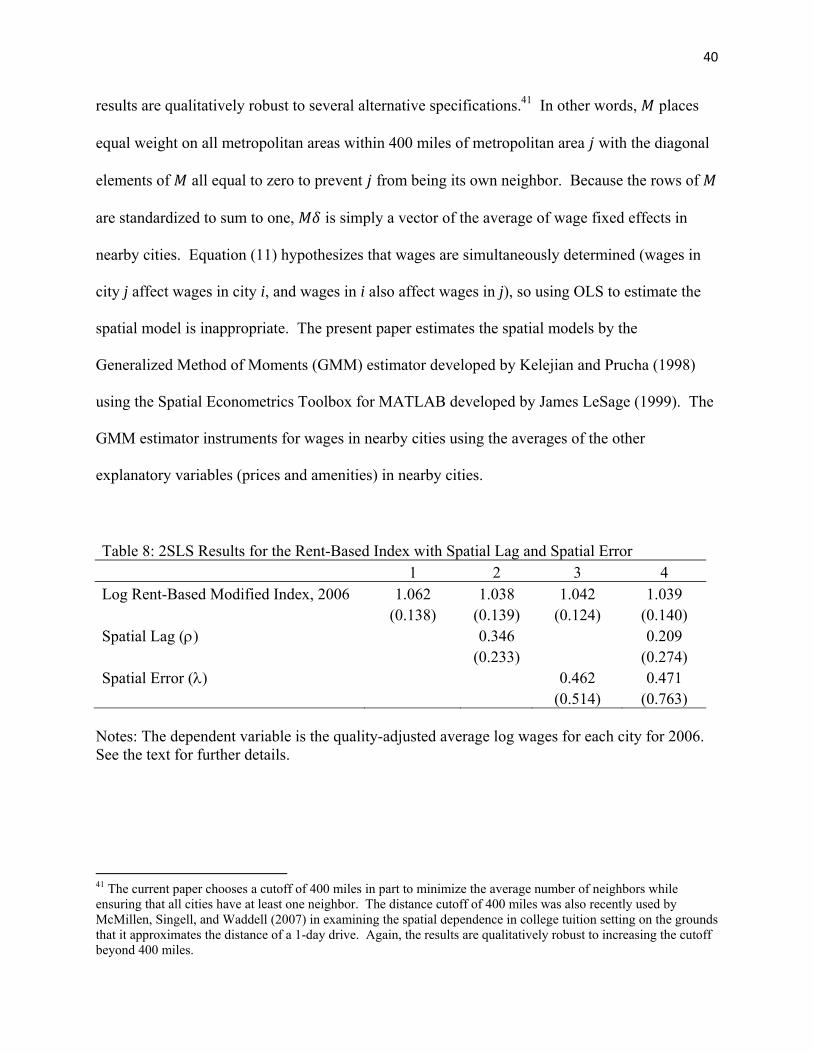
40  

  

results are qualitatively robust to several alternative specifications.41 In other words, places

equal weight on all metropolitan areas within 400 miles of metropolitan area with the diagonal

elements of all equal to zero to prevent from being its own neighbor. Because the rows of

are standardized to sum to one, is simply a vector of the average of wage fixed effects in

nearby cities. Equation (11) hypothesizes that wages are simultaneously determined (wages in

city j affect wages in city i, and wages in i also affect wages in j), so using OLS to estimate the

spatial model is inappropriate. The present paper estimates the spatial models by the

Generalized Method of Moments (GMM) estimator developed by Kelejian and Prucha (1998)

using the Spatial Econometrics Toolbox for MATLAB developed by James LeSage (1999). The

GMM estimator instruments for wages in nearby cities using the averages of the other

explanatory variables (prices and amenities) in nearby cities.

Table 8: 2SLS Results for the Rent-Based Index with Spatial Lag and Spatial Error 1 2 3 4 Log Rent-Based Modified Index, 2006 1.062 1.038 1.042 1.039

(0.138) (0.139) (0.124) (0.140) Spatial Lag (ρ) 0.346 0.209

(0.233) (0.274) Spatial Error (λ) 0.462 0.471    (0.514) (0.763)

Notes: The dependent variable is the quality-adjusted average log wages for each city for 2006. See the text for further details.

                                                            41 The current paper chooses a cutoff of 400 miles in part to minimize the average number of neighbors while ensuring that all cities have at least one neighbor. The distance cutoff of 400 miles was also recently used by McMillen, Singell, and Waddell (2007) in examining the spatial dependence in college tuition setting on the grounds that it approximates the distance of a 1-day drive. Again, the results are qualitatively robust to increasing the cutoff beyond 400 miles.

41  

  

The results are presented in Table 8. The first column reports 2SLS results of (11)

assuming that both 0 and 0.42 This specification essentially differs from the preferred

specification in the first column of Table 4 only in that the city is the level of observation and

each city is given equal weight in Table 8, while in Table 4 the worker was the level of

observation and larger cities were given more weight because they had more workers. The

coefficient on the log of the rent-based price index of 1.062 in the first column is slightly larger

than one, but the difference is not statistically significant. In the second column, we estimate the

spatial lag model that allows for spatial correlation in the dependent variable, but not in the error

term. The wage-price elasticity is 1.038 and not statistically different from unity, and the spatial

lag term is not statistically different from zero. In the third column, we estimate the spatial error

model, which allows for spatial correlation in the errors but not in the dependent variable. The

wage-price elasticity is 1.042 and not statistically different from one and the spatial error

coefficient is not statistically different from zero. In the fourth column, we estimate the general

spatial model that allows for spatial error correlation in both the dependent variable and the error

term. The wage-price elasticity is 1.039 and not statistically different from one, and the

coefficients for the spatial lag and spatial error are again not statistically different from zero.

The results in Table 8, therefore, suggest that wages are not correlated across cities after

controlling for prices and amenities. Consequently, the wage-price elasticity estimate of about

unity is robust to controlling for the possibility of spatial autocorrelation.

7. Empirical Results: The Elasticity between Wages and Housing and Non-Housing Prices

We next separate the price index into housing and non-housing prices and include them

in the wage equation separately. Equation (4) predicts that the wage-price elasticity for a good                                                             42 Throughout this subsection the log of the rent-based price index is instrumented using log gross rents from 2005.

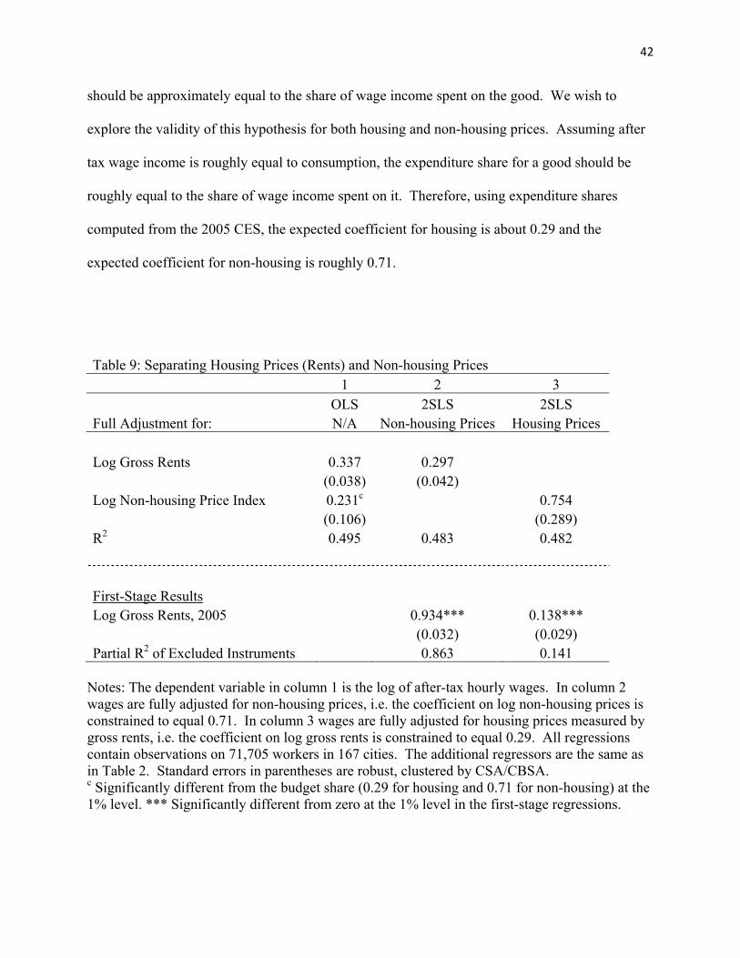
42  

  

should be approximately equal to the share of wage income spent on the good. We wish to

explore the validity of this hypothesis for both housing and non-housing prices. Assuming after

tax wage income is roughly equal to consumption, the expenditure share for a good should be

roughly equal to the share of wage income spent on it. Therefore, using expenditure shares

computed from the 2005 CES, the expected coefficient for housing is about 0.29 and the

expected coefficient for non-housing is roughly 0.71.

Table 9: Separating Housing Prices (Rents) and Non-housing Prices 1 2 3

OLS 2SLS 2SLS Full Adjustment for: N/A Non-housing Prices Housing Prices

Log Gross Rents 0.337 0.297 (0.038) (0.042)

Log Non-housing Price Index 0.231c 0.754 (0.106) (0.289)

R2 0.495 0.483 0.482

First-Stage Results Log Gross Rents, 2005 0.934*** 0.138***

(0.032) (0.029) Partial R2 of Excluded Instruments 0.863 0.141

Notes: The dependent variable in column 1 is the log of after-tax hourly wages. In column 2 wages are fully adjusted for non-housing prices, i.e. the coefficient on log non-housing prices is constrained to equal 0.71. In column 3 wages are fully adjusted for housing prices measured by gross rents, i.e. the coefficient on log gross rents is constrained to equal 0.29. All regressions contain observations on 71,705 workers in 167 cities. The additional regressors are the same as in Table 2. Standard errors in parentheses are robust, clustered by CSA/CBSA. c Significantly different from the budget share (0.29 for housing and 0.71 for non-housing) at the 1% level. *** Significantly different from zero at the 1% level in the first-stage regressions.

43  

  

We first estimate the log wage equation with log gross rents and log non-housing prices

included simultaneously via OLS. As discussed above, measurement error in prices may bias

coefficients toward zero. Alternatively, if non-housing prices are measured with considerable

error, while housing prices are measured with relatively little error, the coefficient on housing

prices could be biased upward. Measurement error would bias the coefficient on non-housing

prices toward zero, and the downward bias in the coefficient for non-housing prices would cause

the coefficient on housing prices to be positively biased because of a partially omitted variable.

In other words, housing prices could pick up some of the effect of non-housing prices. This is

especially problematic given the very high correlation between log gross rents and log non-

housing prices; the raw correlation coefficient between the two is 0.718. The results in column 1

of Table 9 suggest that log gross rents may indeed be picking up some of the effect of log non-

housing prices. The coefficient on log gross rents is 0.337, and is statistically different from zero

at the 1% level but not statistically different from the budget share of 0.29. The coefficient on

log non-housing prices is 0.231, and is statistically different from zero at the 5% level and

statistically different from the budget share of 0.71 at the 1% level.

Ideally, we would like to simultaneously instrument for housing and non-housing prices

to account for measurement error in both. One possibility would be to use lagged values of both

as instruments. However, because measurement error in non-housing prices is likely to be

serially correlated, instrumenting for non-housing prices using its lagged value will not yield

consistent estimates. Instead, we explore estimating the log housing price and log non-housing

price coefficients separately while constraining the other to equal its budget share and

instrumenting using log gross rents for the previous year. This is a hybrid between full

adjustment and partial adjustment for prices used by previous researchers. Constraining one of

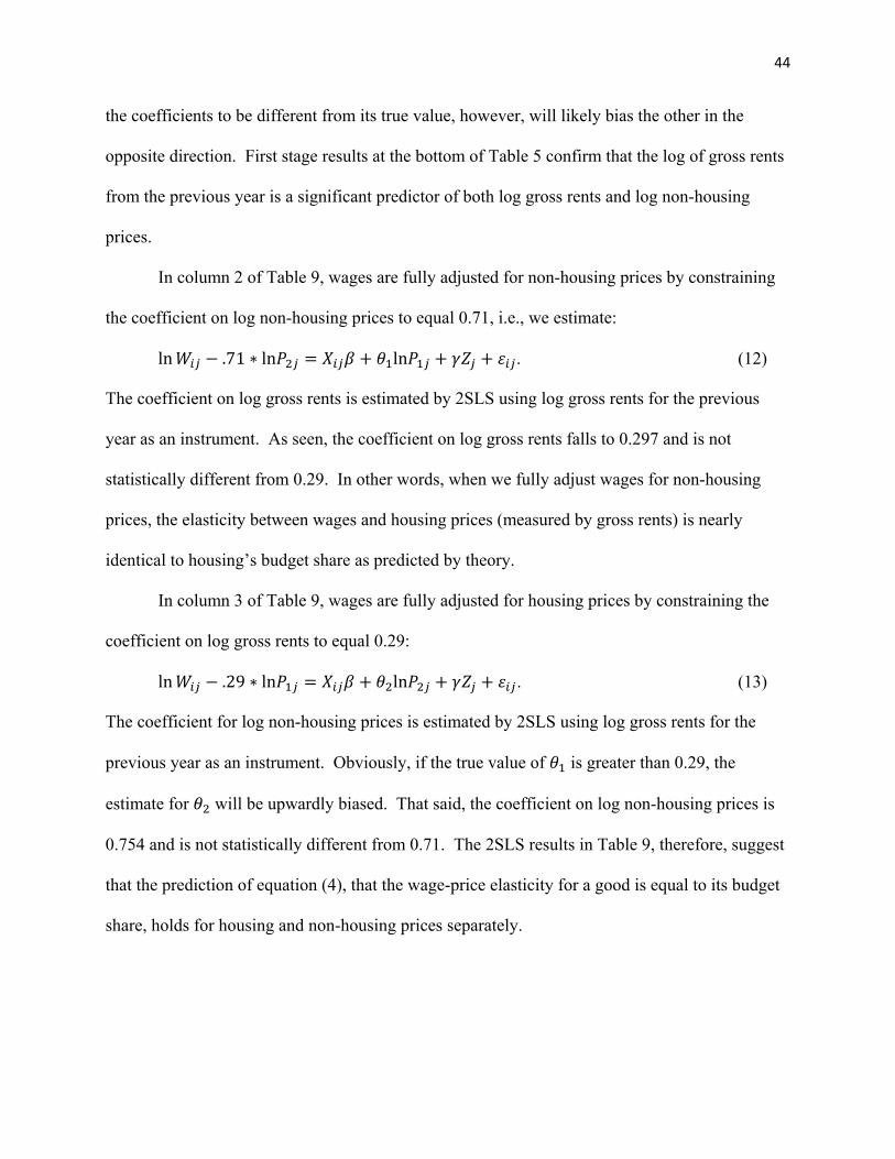
44  

  

the coefficients to be different from its true value, however, will likely bias the other in the

opposite direction. First stage results at the bottom of Table 5 confirm that the log of gross rents

from the previous year is a significant predictor of both log gross rents and log non-housing

prices.

In column 2 of Table 9, wages are fully adjusted for non-housing prices by constraining

the coefficient on log non-housing prices to equal 0.71, i.e., we estimate:

ln .71 ln ln . (12)

The coefficient on log gross rents is estimated by 2SLS using log gross rents for the previous

year as an instrument. As seen, the coefficient on log gross rents falls to 0.297 and is not

statistically different from 0.29. In other words, when we fully adjust wages for non-housing

prices, the elasticity between wages and housing prices (measured by gross rents) is nearly

identical to housing’s budget share as predicted by theory.

In column 3 of Table 9, wages are fully adjusted for housing prices by constraining the

coefficient on log gross rents to equal 0.29:

ln .29 ln ln . (13)

The coefficient for log non-housing prices is estimated by 2SLS using log gross rents for the

previous year as an instrument. Obviously, if the true value of is greater than 0.29, the

estimate for will be upwardly biased. That said, the coefficient on log non-housing prices is

0.754 and is not statistically different from 0.71. The 2SLS results in Table 9, therefore, suggest

that the prediction of equation (4), that the wage-price elasticity for a good is equal to its budget

share, holds for housing and non-housing prices separately.

45  

  

Table 10: Separating Housing Prices (Values) and Non-housing Prices 1 2 3

OLS 2SLS 2SLS Full Adjustment for: NA Non-housing Prices Housing Prices

Log Housing Values 0.143c 0.091 c (0.024) (0.021)

Log Non-housing Price Index 0.165 c -0.641 c (0.132) (0.226)

R2 0.494 0.482 0.484

First-Stage Results Log Housing Values, 2005 0.992*** 0.097***

(0.024) (0.015) Partial R2 of Excluded Instruments 0.949 0.281

Notes: The dependent variable in column 1 is the log of after-tax hourly wages. In column 2 wages are fully adjusted for non-housing prices, i.e. the coefficient on log non-housing prices is constrained to equal 0.77. In column 3 wages are fully adjusted for housing prices measured by housing values, i.e. the coefficient on log housing values is constrained to equal 0.23. All regressions contain observations on 71,705 workers in 167 cities. The additional regressors are the same as in Table 2. Standard errors in parentheses are robust, clustered by CSA/CBSA. c Significantly different from the budget share (0.23 for housing and 0.77 for non-housing) at the 1% level. *** Significantly different from zero at the 1% level in the first-stage regressions.

In Table 10, we reestimate the regressions in Table 9 using quality-adjusted housing

values rather than rents to measure housing prices.43 When we do so, the coefficients on log

housing and log non-housing prices are always significantly less than their budget shares. In

fact, when we fully adjust wages for housing prices measured by housing values in column 3 of

Table 10, the log of the non-housing price index has a significantly negative coefficient. This

reinforces results in the previous section suggesting that housing values are an inappropriate

measure of housing prices.

                                                            43 The expected shares for housing and non-housing now change to 0.23 and 0.77 because housing values do not include utilities and non-housing prices now do.

46  

  

8. Implications for Estimating Implicit Prices of Amenities

The empirical results in this paper have important implications for researchers interested

in estimating the implicit prices of amenities or ranking the quality of life across cities. The

relationship between wages and prices is consistent with the full compensation hypothesis when

we measure housing prices by rents and use lagged rents as an instrument for the general price

level. When we measure housing prices by values, however, the relationship between wages and

prices is highly inconsistent with the full compensation hypothesis, even when using

instrumental variables. This suggests that using housing values along with wages to infer

implicit prices of amenities is likely to produce biased estimates. To illustrate, we estimate

Census division amenity values by regressing log after-tax wages fully adjusted by both the rent-

based modified price index and the baseline price index on eight Census division dummy

variables. These regressions contain individual worker characteristics but no city level controls

other than Census division indicators. The results are presented in columns 1 and 2 of Table

11.44 The implicit price of a division’s amenities is measured as the negative of its division

dummy coefficient for fully adjusted wages. In other words, a low division coefficient indicates

a high value of amenities.

If the true wage-price elasticity is equal to one and the rent-based modified index

measures the general price level across cities without systematic error (but potentially random

error), then the estimates of amenity values by division in column 1 are consistently estimated.45

The estimates in column 1 suggest that the Middle Atlantic, Pacific, and New England (the

                                                            44 We also regressed the log of the rent-based modified index on log gross rents, amenities, region dummies, and city size dummies to obtain predicted values that “net out” potential measurement error. Division dummies estimated for wages fully adjusted using the predicted values of the rent-based modified priced index were nearly identical to those in column 1 using the actual values. 45 The previous two sections argue that there is systematic measurement error within cities over time in non-housing prices. This measurement error, however, can still be unsystematic across cities for a given time period.

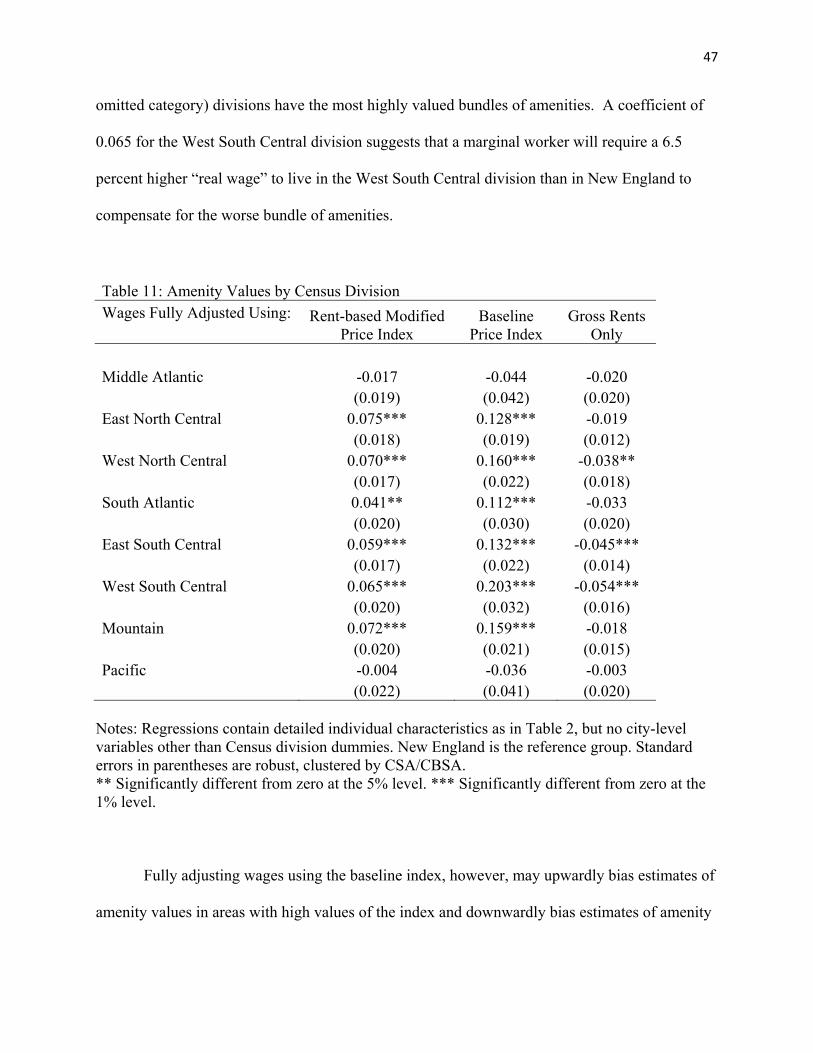
47  

  

omitted category) divisions have the most highly valued bundles of amenities. A coefficient of

0.065 for the West South Central division suggests that a marginal worker will require a 6.5

percent higher “real wage” to live in the West South Central division than in New England to

compensate for the worse bundle of amenities.

Table 11: Amenity Values by Census Division Wages Fully Adjusted Using: Rent-based Modified

Price Index Baseline

Price Index Gross Rents

Only

Middle Atlantic -0.017 -0.044 -0.020 (0.019) (0.042) (0.020)

East North Central 0.075*** 0.128*** -0.019 (0.018) (0.019) (0.012)

West North Central 0.070*** 0.160*** -0.038** (0.017) (0.022) (0.018)

South Atlantic 0.041** 0.112*** -0.033 (0.020) (0.030) (0.020)

East South Central 0.059*** 0.132*** -0.045*** (0.017) (0.022) (0.014)

West South Central 0.065*** 0.203*** -0.054*** (0.020) (0.032) (0.016)

Mountain 0.072*** 0.159*** -0.018 (0.020) (0.021) (0.015)

Pacific -0.004 -0.036 -0.003 (0.022) (0.041) (0.020)

Notes: Regressions contain detailed individual characteristics as in Table 2, but no city-level variables other than Census division dummies. New England is the reference group. Standard errors in parentheses are robust, clustered by CSA/CBSA. ** Significantly different from zero at the 5% level. *** Significantly different from zero at the 1% level.

Fully adjusting wages using the baseline index, however, may upwardly bias estimates of

amenity values in areas with high values of the index and downwardly bias estimates of amenity

48  

  

values in areas with low values of the index. This result follows because housing values are

more dispersed than rents across cities, but rents measure the true user cost of housing. The rank

ordering of division dummies in column 2 is similar to that in column 1, but the estimated

coefficients are much larger. According to wages fully adjusted using the baseline index, a

marginal worker will require a more than 20 percent higher “real wage” to live in the West South

Central than in New England. However, because the baseline index measures housing prices

primarily by housing values, the estimated amenity prices in column 2 are biased.

This paper also has implications for researchers who neglect to include non-housing

prices in measuring the implicit price of amenities.46 Column 3 of Table 11 reports the results of

division dummies for log wages fully adjusted for gross rents (assuming a budget share of 0.29)

but not non-housing prices. The ranking of the coefficients is nearly the opposite of that in

column 1. The West South Central is now the most amenable and the New England and Pacific

divisions are now the worst. These results confirm that ignoring non-housing prices downwardly

biases amenity values for areas with high non-housing prices and upwardly biases amenity prices

for areas with low non-housing prices.47

9. Conclusion

Differences in wages across areas can be partially explained by differences in prices and

amenities. For a given price level, workers are willing to accept lower wages to live and work in

more amenable locations. Controlling for amenities, wages must be higher in high price areas in

order for workers to achieve equal utility across locations. This paper presents a simple model

                                                            46 Researchers including Gabriel et al. (2003), Shapiro (2006) and Albouy (2008b) have begun to incorporate non-housing prices in amenity prices, but this was not generally the case until recently. 47 Interestingly, though, the biases from measuring housing prices by housing values and ignoring non-housing prices are in opposite direction. As a result, measuring housing prices by values and ignoring non-housing prices produces amenity estimates generally between those in column 2 and column 3.

49  

  

that predicts that the elasticity of the wage with respect to the price of a good is proportional to

the share of wage income spent on the good. The model also suggests that if workers’

consumption equals their wage income, then the elasticity between wages and the general price

level should equal one. However, to the extent that the assumptions of the model do not hold,

the actual relationship between wages and prices may differ from that predicted by the model.

Measuring housing prices by rents, we find that the elasticity between wages and the

general price level is nearly identical to one after instrumenting for the general price level using

rents for the previous year. We also present evidence that the wage-price elasticities for housing

and non-housing prices are equal to their budget shares when housing prices are measured by

rents. These results provide empirical evidence in support of the full compensation hypothesis.

Importantly, though, when housing prices are measured by housing values, the elasticity

between wages and the general price level is less than 0.5. The findings in this paper have

important implications for estimating the implicit prices of amenities. Measuring housing prices

by values instead of rents will bias estimates and cause cities with high housing values to have

the relative value of their amenities overstated.

  

50  

ESSAY II: TEACHER SALARIES AND TEACHER UNIONS: A SPATIAL

ECONOMETRIC APPROACH

1. Introduction

Teacher pay is an issue that has received much attention from researchers, politicians,

and the general public. Teacher pay is important for several reasons. For one, state and local

governments spend a large portion of their budgets on education. For the 2005-06 school year,

public school districts in the U.S. had current expenditures per pupil of $9,138, with more than

60 percent of current expenditures going toward teacher salaries and benefits.48 Teacher pay is

also important because of the sheer number of public school teachers in the U.S. In 2006, full-

time equivalent employment of elementary and secondary teachers by state and local

governments was more than 4.6 million, making teachers by far the largest group of state and

local government employees.49 Teacher pay is also likely to affect the ability of school districts

to recruit and retain quality teachers as suggested by a sizable literature in education finance

(e.g., Murnane and Olsen 1989, 1990; Figlio 1997, 2002; Clotfelter et al. 2008)

In this paper, we use a spatial econometric framework to examine the effects of teacher

unions and other school district characteristics on teacher salaries. While a large literature has

investigated the determinants of teacher salaries, only a handful of these studies have used spatial

econometric methods to account for spatial dependence in teacher salaries. The few studies that

do so provide analysis of individual states and give little attention to the effects of unions. To

the researcher’s knowledge, this paper is the first to examine teacher salaries in a spatial

econometric framework for the 48 contiguous U.S. states.

                                                            48 Source: U.S. Census Bureau, Governments Division 49 Source: U.S. Census Bureau, Governments Division

51  

 

Unions are also likely to affect school districts in ways other than increasing teacher

salaries. For one, unions are likely to affect the level of fringe benefits that teachers receive as

part of their compensation package. Unions are likely to work toward better health insurance

benefits, better pension benefits, and greater job security for the teachers they represent. Unions

may also affect other school district characteristics such as the student-teacher ratio and the level

and composition of non-instructional expenditures. Perhaps most importantly, the overall

influence of unions may affect the amount that students learn through altering inputs into the

production of education and by empowering teachers.50 The current paper, however, focuses on

the effect of unions on the salaries that teachers are paid. Additional effects that unions might

have on school districts are beyond the scope of this paper.

The results in this paper confirm that teacher salaries are positively affected by salaries in

nearby districts even after controlling for several other variables that explain teacher salaries.

We find that a one percent increase in the average salary of experienced teachers in nearby

districts increases salaries for experienced teachers in a given district by between 0.51 and 0.68

percent. For beginning teachers the effect of salaries in nearby districts is even stronger with

estimates between 0.85 and 0.92 percent. Furthermore, accounting for spatial dependence

produces estimates for several variables that differ considerably from models that ignore the

spatial relationship. Incorporating union spillovers at the state level, we find that collective

bargaining and union membership density increase the salaries of experienced teachers by as

much as 16 and 21 percent, respectively, but the estimated effects on the salaries of beginning

teachers are much smaller. This result is consistent with predictions from a median voter model.

                                                            50 The overall effect of unions on learning is unclear a priori. For example, unions may increase the level of inputs, but decrease the efficiency with which those inputs are used. Hoxby (1996) finds that unions have a negative overall effect on student performance.

52  

 

The remainder of the paper is organized as follows. The next section reviews the

literature on teacher salaries, paying specific attention to studies that focus on the effects of

unions and studies that examine teacher salaries using a spatial econometric framework. Section

3 presents the empirical model, and section 4 discusses data. Empirical results are presented in

section 5 and a brief summary is provided in a concluding section.

2. Theory and Previous Literature

Numerous research studies investigate the determinants of teacher salaries. Many of

these focus specifically on how teacher unions affect teacher salaries.51 Theory suggests that the

effect of unions on the level and structure of teacher salaries should be determined by union

goals and bargaining power. Union goals are most readily understood by reference to some form

of a median voter model, discussed below. Bargaining power derives from numerous factors,

including state collective bargaining laws, the extent of organizing, political support, the

structure of districts (which affects employer concentration), and financial ability to pay.

Previous empirical studies typically regress the log of average salaries on union activity

measures and other characteristics of the school district and local labor market. Results vary

considerably across studies in part due to the measures of teacher salaries and union activity that

are used. A few studies find little to no effect, but most recent studies find at least a modest

positive effect.52 Hoxby’s (1996) finding of a roughly five percent effect of collective

bargaining representation on average teacher salaries is fairly representative of most studies.

                                                            51 Early reviews of the literature are provided by Lipsky (1982), Ehrenberg and Schwarz (1986), and Freeman (1986). 52 In a recent paper Lovenheim (2008) finds collective bargaining coverage to have virtually no effect on average teacher salaries in three Midwestern states. His results, however, also suggest that collective bargaining is associated with increased enrollment and teacher employment in these states. If the increased employment decreased the average level of experience and education in these districts, then the effect of unionization on average salaries may be downwardly biased.

53  

 

Still, at least a few studies find union effects as large as 20 percent of wages (e.g., Baugh and

Stone 1982; Zwerling and Thomason 1995).

A few studies also recognize that teacher unions might differentially affect the salaries of

teachers within a given district. In other words, unions not only affect the average level of

salaries but also the distribution of salaries within a district. Holmes (1976) finds that unions

increase both the return to experience and the return to education within a district. Similarly,

Delaney (1985) finds that collective bargaining increases the salary differential between

experienced teachers and inexperienced teachers. Zwerling and Thomason (1995) and Lentz

(1998) also find that while unions have a positive and significant effect on the salaries of

teachers earning the highest salary in a district, unions have a small (though still positive) and

insignificant effect on the lowest salary in a district. Babcock and Engberg (1999) and Ballou

and Podgursky (2002) also suggest that the average levels of teaching experience and education

in a district affect the returns to experience and education as well.

The effect of teacher unions on intra-district salary differentials is often explained by

appealing to the median voter model. Virtually all public school districts, including those

without collective bargaining, pay teachers according to a salary schedule that maps salary to

teaching experience and education. In the absence of union pressures, district administrators

may dictate a salary schedule that is more appealing to marginal teachers than median teachers,

with the marginal teachers being those at the tails of the distributions of experience and

education. However, the union’s preferred salary structure may be heavily influenced by the

preferences and hence characteristics (i.e. experience and education) of the median teacher in the

district. According to data tabulated from the 1999-2000 Schools and Staffing Survey (SASS)

54  

 

Teacher Survey, about half of public school teachers in the U.S. had advanced degrees and the

average experience was about fifteen years.

Because there are multiple dimensions to union contracts (returns to experience, returns

to education, the level of fringe benefits, etc.), the median voter model may not adequately

explain the salary determination process within districts. Having multiple choice variables

means that there is likely no single median voter whose preferences are decisive. Instead, it may

be useful to more generally view union preferences as resulting from a majority coalition of

teachers. Union cohesion may even require that there be a super-majority coalition. Even with

multiple choices to be made, though, it still seems likely that teachers with median levels of

experience and education will be important members of the majority coalition and will push for a

salary structure that benefits them. Teachers with little or no experience may be the ones most

likely to be left out of the majority coalition for several reasons. First, inexperienced teachers

may be less likely to be members of the union and less likely to be active in the union when they

are members. Additionally, union contracts are often negotiated months or even years in

advance of the school year for which they apply. As a result, the very newest teachers never had

a vote on how the salary schedule would be structured. School district administrators, however,

are likely to be sensitive to market conditions for new school teachers since this is when teachers

are most mobile. Thus, we might expect unionized school districts with strong union bargaining

power to respond to the preferences of experienced (median voter) teachers, whereas nonunion

districts or union districts where bargaining power is weak may be more responsive to market

conditions for new teachers.

It is reasonable to expect that unions might increase the salary differential between

beginning and experienced teachers even absent the median voter mechanism. Entry-level

55  

 

teachers searching for jobs are substantially more mobile than experienced teachers. Hence,

starting salaries among nearly all districts must be reasonably competitive in order to attract

teachers of any given quality. As teacher mobility decreases with experience and district-

specific tenure employer monopsony power may increase, leading to salaries below competitive

levels for experienced (but not beginning) teachers in districts with low mobility. Union

bargaining power can offset this monopsony power, thus creating a union wage gap for

experienced teachers (i.e., higher salaries for experienced teachers in union than in nonunion

districts), while at the same time having little effect on starting salaries for union relative to

nonunion teachers.

Unions might also increase the salary differential between teachers with and without

advanced degrees. This shifting in the salary structure may even result in less experienced

teachers having lower salaries than would be the case in the absence of union negotiations. Such

a “deferred payment” scheme should attract teachers willing to accept low initial salaries based

on the expectation that they will receive subsequent rewards for tenure and an advanced degree.

Chambers (1977), Delaney (1985) and Zwerling and Thomason (1995) suggest that union

activity in a district produces positive wage spillovers in nearby districts. In fact, all three

studies suggest that the union spillover effect on wages is larger than the direct effect. A few

more recent studies suggest that teacher wage spillovers may be more direct. Wagner and Porter

(2000), Greenbaum (2002), Babcock, Engberg and Greenbaum (2005), and Millimet and

Rangaprasad (2007) find using spatial econometric methods that teacher salaries in a district are

positively influenced by teacher salaries in nearby districts.53 In other words, teacher salaries

                                                            53 Ready and Sandver (1993) also find that salaries are correlated with salaries in nearby districts. However, their analysis is based on OLS and does not account for the simultaneity of salaries for districts in close proximity. As will be discussed in more detail in the next section, appropriate spatial methods account for the simultaneity in teacher salaries using instrumental variables.

56  

 

appear to be spatially dependent, at least in the states considered in these studies.54 However,

each of these studies examines a single state and with the exception of Babcock et al. (2005) do

not generally focus on the effects of unions. The current paper makes an important contribution

to the literature by using a national level dataset to examine the effect of unions on teacher

salaries in a spatial econometric framework.

3. Empirical Model

Most previous studies of the determinants of teacher salaries do not account for spatial

dependence. The usual estimation equation in these studies is given by:

, (1)

where is an 1 vector of teacher salaries (usually measured in logs), is an matrix of

explanatory variables, is a 1 vector of parameters, and is a mean zero error term

assumed to be i.i.d. across observations.

In this paper we consider the possibility that teacher salaries are spatially correlated after

controlling for other determinants of teacher salaries. The primary concern is that teacher

salaries in a district may be affected by teacher salaries in neighboring districts. This type of

spatial dependence is likely to occur for at least two reasons. First, school districts likely

compete with nearby districts for quality teachers. If one district offers a salary substantially

below that of nearby districts, they will have difficulty hiring and retaining quality teachers.

Thus school district administrators have incentives to keep teacher salaries, especially starting

salaries, competitive with salaries in nearby districts. Similarly, comparisons of salaries in

nearby districts are almost always used in contract negotiations between administrators and

                                                            54 Wagner and Porter (2000) examine school districts in Ohio; Greenbaum (2002) and Babcock et al. (2005) examine districts in Pennsylvania; and Millimet and Prangasad (2007) examine districts in Illinois.

57  

 

teacher unions. Thus spatial dependence in teacher salaries seems quite plausible. If there is

spatial dependence in the dependent variable then methods that do not account for this are likely

to produce inconsistent coefficient estimates (Anselin, 1988). A second concern is that there

may be spatial correlation in the error term, say from spatially correlated measurement error in

an explanatory variable (e.g., the county unemployment rate) for nearby districts (Kalenkoski

and Lacombe 2008). Failing to account for spatial correlation in the error term may result in

standard errors that are inconsistently estimated.

The spatial model can be represented by:

(2)

,

where is an weighting matrix that specifies the structure of the spatial correlation, and

are spatial autocorrelation coefficients for the dependent variable and the error term,

respectively, and is a mean zero error term that is i.i.d. across observations. In the current

paper, is specified based on the distance between school districts. For row i of matrix ,

districts that are more than 50 miles away from i are given zero weight. In other words districts

are only considered neighbors if they are within 50 miles of each other. Districts within 50 miles

of i are weighted based on their inverse distance to i, so that nearer districts are given more

weight than districts further away.55 The choice of this weighting matrix reflects the assumption

that salaries in a district are most strongly affected by salaries in other districts that are closest to

it and that the effect is attenuated with distance. The matrix is also structured so that the

elements in each row sum to unity and all diagonal elements are equal to zero.56 In other words,

is a distance-weighted average of teacher salaries in nearby districts, and is a distance-                                                            55 Alternatively, we could equally weight all districts within 50 miles. The results are not considerably affected by this modification to the weighting scheme. 56 The zero diagonals reflect the assumption that a district cannot be its own neighbor.

58  

 

weighted average of the error terms in nearby districts. We can also estimate a spatial model that

allows for a more robust specification of the spatial dependence in the errors. Specifically,

instead of assuming that as in equation (2), we can estimate an equation with a

spatially lagged dependent variable while allowing for error correlation or clustering within

groups.57 In the empirical analysis to follow we estimate both equations that model the spatial

error correlation as in equation (2) and equations that include a spatially lagged dependent

variable, then account for cross-sectional dependence in the error terms.58

It should be clear that teacher salaries in neighboring districts may be simultaneously

determined. Salaries in district j affect salaries in district i, but salaries in district i also affect

salaries in district j. Because of the simultaneity involved, using Ordinary Least Squares (OLS)

to estimate the spatial model is inappropriate. Instead, instrumental variable methods should be

used. More specifically, the present paper estimates the spatial models by the Generalized

Method of Moments (GMM) estimator developed by Kelejian and Prucha (1998) using the

Spatial Econometrics Toolbox for MATLAB developed by James LeSage and described in

LeSage (1999). The GMM estimator instruments for using and as instruments.

In other words, the estimator instruments for salaries in nearby districts using the distance-

weighted averages of the other explanatory variables in nearby districts along with the distance-

weighted averages of their neighbors’ neighbors’ characteristics.

Kelejian and Prucha (1998) outline the conditions under which the GMM estimator

provides consistent estimates. While the reader is referred to Kelejian and Prucha (1998) for a

more formal discussion, a brief discussion of some of these assumptions is useful. First, the

                                                            57 Some spatial econometric studies also estimate a model that assumes that there is spatial correlation in the errors but not in the dependent variable, i.e. 0. Because we have reason to believe that teacher salaries are directly affected by teacher salaries in neighboring districts, the spatial error model that assumes no spatial correlation in the dependent variable seems inappropriate. 58 Wooldridge (2003, 2006) provides a discussion of the use of cluster methods in applied econometrics.

59  

 

diagonal elements of are zero. Additionally, is nonsingular, where is an

identity matrix, and the absolute values of and are each less than one. The row and column

sums of and are bounded in absolute value, where is an

inverse matrix. Additionally, the matrix of exogenous regressors and the matrix of instruments

have full column rank. It must also be the case that at least one of the nonconstant exogenous

regressors in the model has a nonzero effect on . In other words, we need the instruments to

predict in order for the model to be identified. Again, for a more complete discussion and a

proof of the consistency of the estimator, the reader is referred to Kelejian and Prucha (1998).

The marginal effects of the exogenous variables in equation (2) are not equal to the

parameters in vector . Rewriting equation (2) as:

, (3)

is an identity matrixit is easily seen that the partial derivative of with respect to a single

exogenous variable ( 1) is given by:

/

/ / … // / … /

/ / … /

. (4)

Therefore, the marginal effect on teacher salaries of an explanatory variable such as union

activity is . If is measured at the district level, then the average marginal effect

of an increase in in a district on teacher salaries in that district is equal to times the

average of the diagonal elements of the matrix. More formally, setting

… …

…

, (5)

60  

 

the average marginal effect of an increase in in a district on teacher salaries in that district is

∑ . If is measured at a level of concentration larger than the district, such as the

state, then the average marginal effect of an increase in at the state level on teacher salaries in

a district is equal to ∑ ∑ , where is equal to one if i = j or if i and j are in the

same state and are defined as neighbors according to the spatial weight matrix (i.e. within 50

miles of each other in this paper). Because is measured at the state level, the marginal effect

of on for district i includes not only the direct effect of district i but also the indirect effects

of “neighboring” districts in the same state. Kim, Phipps, and Anselin (2003) show that if

does not vary among neighboring districts (e.g., the variable is measured at the state level and all

neighbors are in the same state), then the average marginal effect of a unit increase in is equal

to / 1 . We can think of ∑ ∑ as a spatial multiplier with both ∑

and 1/ 1 as special cases. In the results section, we report both the coefficient estimates

and the average marginal effects for the exogenous variables in the spatial models.

4. Data

The primary data used in this analysis come from the school district survey of the 1999-

2000 Schools and Staffing Survey (SASS) conducted by the National Center for Education

Statistics (NCES) and completed by school district administrators. We examine school districts

in the 48 contiguous U.S. states. Additional data are obtained from the NCES Common Core of

Data (CCD), the NCES Comparable Wage Index (CWI) which measures the wages in the local

labor market of occupations comparable to teaching, the NCES School District Demographics

System (SDDS), and the Bureau of Labor Statistics (BLS) Local Area Unemployment Statistics

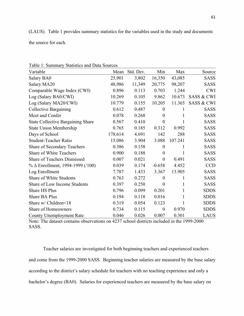
61  

 

(LAUS). Table 1 provides summary statistics for the variables used in the study and documents

the source for each.

Table 1: Summary Statistics and Data Sources Variable Mean Std. Dev. Min Max SourceSalary BA0 25,901 3,802 16,350 43,085 SASSSalary MA20 48,986 11,349 20,775 98,207 SASSComparable Wage Index (CWI) 0.896 0.113 0.703 1.244 CWILog (Salary BA0/CWI) 10.269 0.105 9.862 10.673 SASS & CWILog (Salary MA20/CWI) 10.779 0.155 10.205 11.365 SASS & CWICollective Bargaining 0.612 0.487 0 1 SASSMeet and Confer 0.078 0.268 0 1 SASSState Collective Bargaining Share 0.567 0.410 0 1 SASSState Union Membership 0.765 0.185 0.312 0.992 SASSDays of School 178.614 4.691 142 288 SASSStudent-Teacher Ratio 15.086 3.904 3.088 107.241 SASSShare of Secondary Teachers 0.386 0.158 0 1 SASSShare of White Teachers 0.900 0.188 0 1 SASSShare of Teachers Dismissed 0.007 0.021 0 0.491 SASS% Δ Enrollment, 1994-1999 (/100) 0.039 0.174 -0.658 4.452 CCDLog Enrollment 7.787 1.433 3.367 13.905 SASSShare of White Students 0.763 0.272 0 1 SASSShare of Low Income Students 0.397 0.250 0 1 SASSShare HS Plus 0.796 0.099 0.201 1 SDDSShare BA Plus 0.194 0.118 0.016 1 SDDSShare w/ Children<18 0.319 0.054 0.123 1 SDDSShare of Homeowners 0.734 0.115 0 0.970 SDDSCounty Unemployment Rate 0.046 0.026 0.007 0.301 LAUSNote: The dataset contains observations on 4237 school districts included in the 1999-2000 SASS.

Teacher salaries are investigated for both beginning teachers and experienced teachers

and come from the 1999-2000 SASS. Beginning teacher salaries are measured by the base salary

according to the district’s salary schedule for teachers with no teaching experience and only a

bachelor’s degree (BA0). Salaries for experienced teachers are measured by the base salary on

62  

 

the district’s salary schedule for teachers with 20 years of teaching experience and a master’s

degree related to the teaching field (MA20).59 Beginning teachers in the sample have a mean

salary of $25,901 while the mean salary for experienced teachers is nearly twice that. There is

also considerably more variation in the salaries of experienced teachers. The standard deviation

in salaries for experienced teachers is nearly three times that of beginning teachers.

For both beginning and experienced teachers, the dependent variable in the analysis

below is measured as the log of the reported salary relative to the level of comparable wages of

workers in the same labor market using the CWI (Taylor and Fowler 2006). In other words, if

is the nominal salary for experienced teachers, is the nominal salary for beginning

teachers, and is the value for the comparable wage index, then the dependent variable for

experienced teachers is ln / and the dependent variable for beginning teachers is

ln / . Comparable wages provide a good measure of the relative cost of living in a

particular labor market and also serve as a proxy for the opportunity cost of teaching in a given

market (Stoddard 2005). Without measuring teacher salaries relative to comparable wages,

spatial autocorrelation could in part result from salaries being high for all districts in expensive

labor markets and low for districts in inexpensive labor markets. Measuring teacher salaries

relative to comparable wages, any spatial autocorrelation that we find will be more than just the

result of nearby districts responding similarly to similar living costs.

The regression analysis below includes a number of important explanatory variables.

The effect of unions is given considerable emphasis in this paper and union activity is measured

in three different ways. We first measure union activity by two mutually exclusive indicator

                                                            59 Individual teachers are sometimes paid amounts above that required by the salary schedule for special credentials or extra duties such as coaching a sports team. However, the salary measures in this paper are for the base salary in the district and do not include extra pay for special credentials or extra duties.

63  

 

variables for collective bargaining and the presence of a meet and confer agreement in the

district. Meet and confer agreements are not binding on school districts and are considered to be

a much weaker form of union activity than collective bargaining. As seen in Table 1, more than

61 percent of the districts engage in collective bargaining, and another eight percent have meet

and confer agreements. Thus roughly 31 percent of districts have neither. Previous literature has

suggested that union activity in neighboring districts has important spillover effects, and the next

two measures of union activity incorporate union spillovers. The second measure of union

activity is the share of districts in a state with a collective bargaining agreement.60 If collective

bargaining has important spillovers effects for teacher salaries in nearby districts, the effect for

the state collective bargaining share should be greater than the effect for the collective bargaining

indicator variable. The third measure of union activity is the percentage of teachers in a state

who are members of a teacher union, which also incorporates union spillovers. Unfortunately,

union membership at the district level is not available, so we cannot compare the effects of state

membership density to that of district membership density. Though the second and third

measures of union activity both incorporate union spillovers, they are different measures and

could produce somewhat different results.61

The analysis also includes a number of other important variables thought to affect teacher

salaries. Teachers are expected to require greater compensation for longer school years, so the

number of days in the school year is expected to have a positive sign. Teachers likely prefer

                                                            60 We also experimented with measuring union activity by the share of districts in a state with a meet and confer agreement and the share of districts in a state with any sort of agreement (e.g., collective bargaining or meet and confer). The results for the share of districts with meet and confer was either negative or small and insignificant, consistent with later results suggesting that meet and confer agreements do not increase teacher salaries. The results for the share with any agreement variable are qualitatively similar to the results for the share with collective bargaining. These results are available from the author. 61 One limitation to the current paper is that all of the union activity measures are treated as exogenous. If union activity is in fact endogenous because of simultaneity, omitted variables, or measurement error, coefficient estimates could be biased and inconsistent.

64  

 

smaller classes, so the student-teacher ratio is expected to have a positive coefficient. Secondary

teaching may be more difficult or require greater skills, so the share of secondary teachers is

expected to have a positive coefficient. The share of teachers who are white is included as a

control, but the expected effect is somewhat unclear. Districts that have dismissed relatively

large numbers of teachers recently may have a low need for teachers and pay less competitive

salaries. Districts that have experienced increased enrollments over the previous five years are

expected to have a high demand for teachers and be willing to pay higher relative salaries.

Similarly, larger districts are expected to pay more competitive salaries, and the log of district

enrollment is expected to have a positive coefficient. Teachers may require compensating

differentials to teach students from disadvantaged backgrounds, so the share of students who are

white is expected to have a negative effect, while the share of students that are low income as

measured by free or reduced lunch eligibility is expected to have a positive effect. More

educated residents are thought to have greater demand for education, so the share of adults (age

25+) living in the district with at least a high school degree and the share of adults with at least a

bachelor’s degree are both expected to have positive coefficients. Residents with children are

expected to demand greater spending on education, so the share of households with at least one

child under age 18 is expected to have a positive effect. Renters may be more likely than

homeowners to support spending on education, so the share of households who are homeowners

is expected to have a negative effect. Finally, the unemployment rate in the county in which the

district is located is included to capture local labor market conditions. Higher unemployment is

likely to make it more difficult to find a well-paying career outside of teaching and is expected to

have a negative effect on teacher salaries.

65  

 

5. Results

We begin by estimating equation (1) using OLS. However, because social comparisons

are likely to be important in the determination of teacher salaries and because previous research

has found evidence of spatial dependence in teacher salaries, the preferred methods account for

spatial correlation in the dependent variable. We next estimate the spatial model of equation (2)

using GMM, which also models spatial dependence in the error term. We then estimate the

equation that includes a spatially lagged dependent variable with standard errors clustered by

state. Results that measure union activity by collective bargaining and meet and confer indicator

variables are discussed first and reported in Tables 2 and 3 for experienced and beginning

teachers, respectively. Tables 4 and 5 reestimate the equations in Tables 2 and 3 measuring

union activity by the share of districts in the state with a collective bargaining agreement. Tables

6 and 7 reestimate the equations in Tables 2 and 3 measuring union activity by the share of

teachers in the state who are members of a teacher union. For exogenous variables in the spatial

models, we report coefficient estimates, standard errors in parentheses, and average marginal

effects in brackets computed as described above in Section 3.62 When discussing magnitudes for

these variables, we will focus on the marginal effects.63

Spatial Correlation Coefficients

The results confirm that salaries are spatially dependent for both experienced teachers

and beginning teachers even after controlling for many other variables that explain teacher

salaries. The spatial models that also model the spatial error correlation in column 2 of Tables 2

and 3 report statistically significant spatial lag coefficients ( ) of 0.68 and 0.92 for experienced

and beginning teachers, respectively. The larger coefficient for beginning teachers is likely due                                                             62 For ease of discussion, we often refer to the average marginal effect simply as the marginal effect. 63 Note that coefficient estimates in the OLS equations can be directly interpreted as marginal effects because of the linearity assumption.

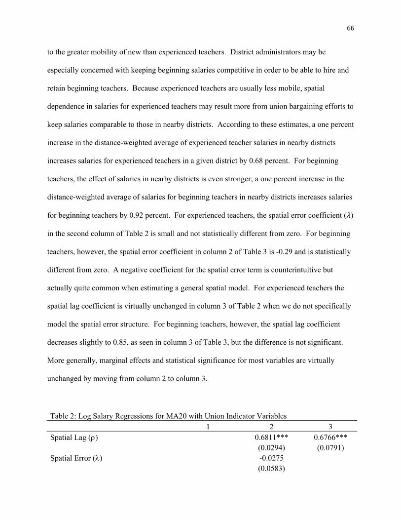
66  

 

to the greater mobility of new than experienced teachers. District administrators may be

especially concerned with keeping beginning salaries competitive in order to be able to hire and

retain beginning teachers. Because experienced teachers are usually less mobile, spatial

dependence in salaries for experienced teachers may result more from union bargaining efforts to

keep salaries comparable to those in nearby districts. According to these estimates, a one percent

increase in the distance-weighted average of experienced teacher salaries in nearby districts

increases salaries for experienced teachers in a given district by 0.68 percent. For beginning

teachers, the effect of salaries in nearby districts is even stronger; a one percent increase in the

distance-weighted average of salaries for beginning teachers in nearby districts increases salaries

for beginning teachers by 0.92 percent. For experienced teachers, the spatial error coefficient ( )

in the second column of Table 2 is small and not statistically different from zero. For beginning

teachers, however, the spatial error coefficient in column 2 of Table 3 is -0.29 and is statistically

different from zero. A negative coefficient for the spatial error term is counterintuitive but

actually quite common when estimating a general spatial model. For experienced teachers the

spatial lag coefficient is virtually unchanged in column 3 of Table 2 when we do not specifically

model the spatial error structure. For beginning teachers, however, the spatial lag coefficient

decreases slightly to 0.85, as seen in column 3 of Table 3, but the difference is not significant.

More generally, marginal effects and statistical significance for most variables are virtually

unchanged by moving from column 2 to column 3.

Table 2: Log Salary Regressions for MA20 with Union Indicator Variables 1 2 3 Spatial Lag (ρ) 0.6811*** 0.6766***

(0.0294) (0.0791) Spatial Error (λ) -0.0275

(0.0583)

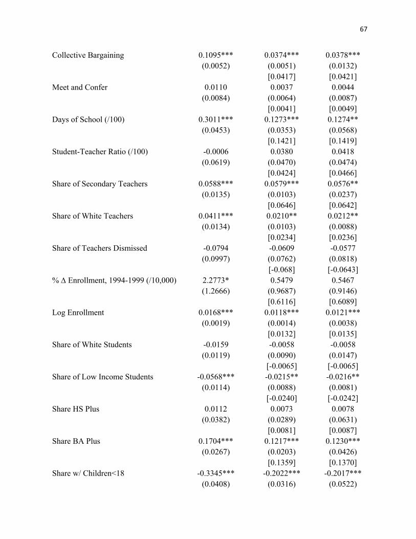
67  

 

Collective Bargaining 0.1095*** 0.0374*** 0.0378*** (0.0052) (0.0051) (0.0132)

[0.0417] [0.0421] Meet and Confer 0.0110 0.0037 0.0044

(0.0084) (0.0064) (0.0087) [0.0041] [0.0049]

Days of School (/100) 0.3011*** 0.1273*** 0.1274** (0.0453) (0.0353) (0.0568)

[0.1421] [0.1419] Student-Teacher Ratio (/100) -0.0006 0.0380 0.0418

(0.0619) (0.0470) (0.0474) [0.0424] [0.0466]

Share of Secondary Teachers 0.0588*** 0.0579*** 0.0576** (0.0135) (0.0103) (0.0237)

[0.0646] [0.0642] Share of White Teachers 0.0411*** 0.0210** 0.0212**

(0.0134) (0.0103) (0.0088) [0.0234] [0.0236]

Share of Teachers Dismissed -0.0794 -0.0609 -0.0577 (0.0997) (0.0762) (0.0818)

[-0.068] [-0.0643] % Δ Enrollment, 1994-1999 (/10,000) 2.2773* 0.5479 0.5467

(1.2666) (0.9687) (0.9146) [0.6116] [0.6089]

Log Enrollment 0.0168*** 0.0118*** 0.0121*** (0.0019) (0.0014) (0.0038)

[0.0132] [0.0135] Share of White Students -0.0159 -0.0058 -0.0058

(0.0119) (0.0090) (0.0147) [-0.0065] [-0.0065]

Share of Low Income Students -0.0568*** -0.0215** -0.0216** (0.0114) (0.0088) (0.0081)

[-0.0240] [-0.0242] Share HS Plus 0.0112 0.0073 0.0078

(0.0382) (0.0289) (0.0631) [0.0081] [0.0087]

Share BA Plus 0.1704*** 0.1217*** 0.1230*** (0.0267) (0.0203) (0.0426)

[0.1359] [0.1370] Share w/ Children<18 -0.3345*** -0.2022*** -0.2017***

(0.0408) (0.0316) (0.0522)

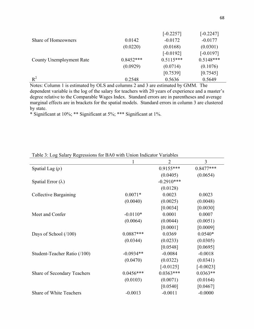
68  

 

[-0.2257] [-0.2247] Share of Homeowners 0.0142 -0.0172 -0.0177

(0.0220) (0.0168) (0.0301) [-0.0192] [-0.0197]

County Unemployment Rate 0.8452*** 0.5115*** 0.5148*** (0.0929) (0.0714) (0.1076)

[0.7539] [0.7545] R2 0.2548 0.5636 0.5649

Notes: Column 1 is estimated by OLS and columns 2 and 3 are estimated by GMM. The dependent variable is the log of the salary for teachers with 20 years of experience and a master’s degree relative to the Comparable Wages Index. Standard errors are in parentheses and average marginal effects are in brackets for the spatial models. Standard errors in column 3 are clustered by state. * Significant at 10%; ** Significant at 5%; *** Significant at 1%.

Table 3: Log Salary Regressions for BA0 with Union Indicator Variables 1 2 3 Spatial Lag (ρ) 0.9155*** 0.8477***

(0.0405) (0.0654) Spatial Error (λ) -0.2910***

(0.0128) Collective Bargaining 0.0071* 0.0023 0.0023

(0.0040) (0.0025) (0.0048) [0.0034] [0.0030]

Meet and Confer -0.0110* 0.0001 0.0007 (0.0064) (0.0044) (0.0051)

[0.0001] [0.0009] Days of School (/100) 0.0887*** 0.0369 0.0540*

(0.0344) (0.0233) (0.0305) [0.0548] [0.0695]

Student-Teacher Ratio (/100) -0.0934** -0.0084 -0.0018 (0.0470) (0.0322) (0.0341)

[-0.0125] [-0.0023] Share of Secondary Teachers 0.0456*** 0.0363*** 0.0363**

(0.0103) (0.0071) (0.0164) [0.0540] [0.0467]

Share of White Teachers -0.0013 -0.0011 -0.0000

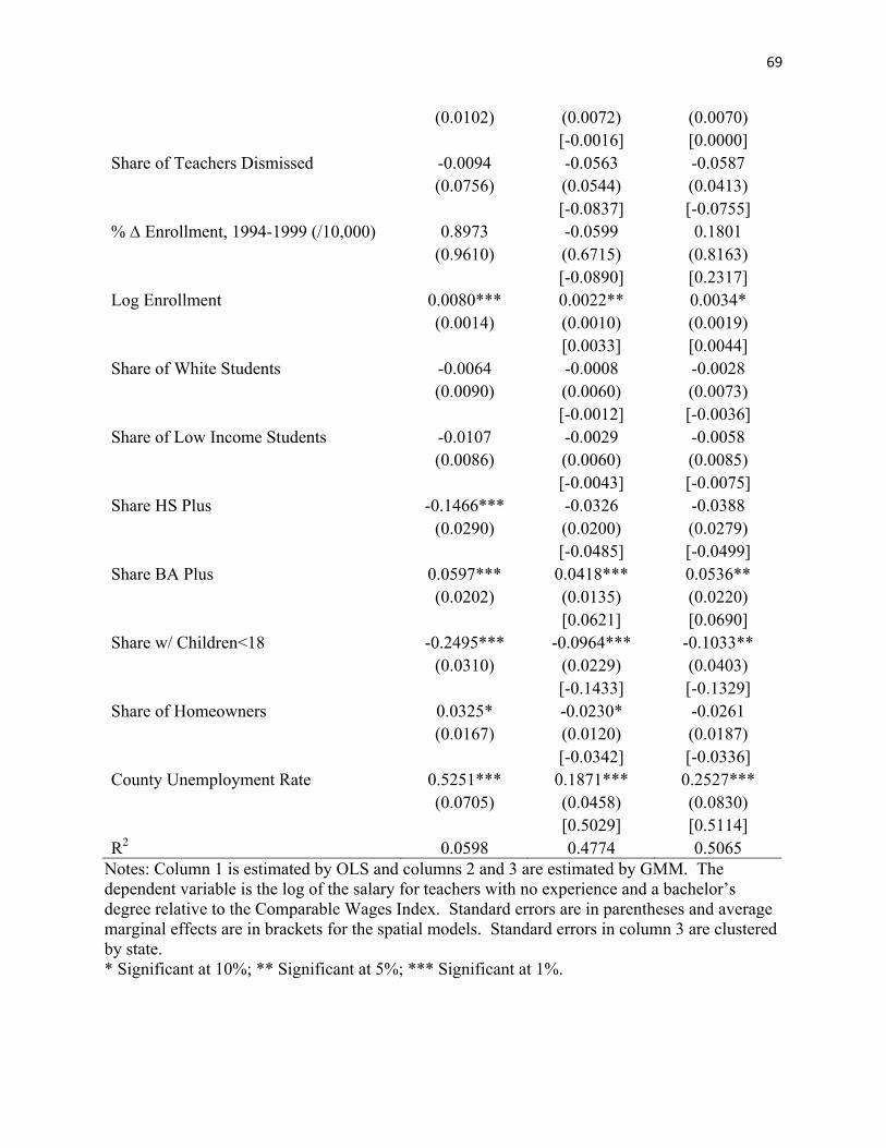
69  

 

(0.0102) (0.0072) (0.0070) [-0.0016] [0.0000]

Share of Teachers Dismissed -0.0094 -0.0563 -0.0587 (0.0756) (0.0544) (0.0413)

[-0.0837] [-0.0755] % Δ Enrollment, 1994-1999 (/10,000) 0.8973 -0.0599 0.1801

(0.9610) (0.6715) (0.8163) [-0.0890] [0.2317]

Log Enrollment 0.0080*** 0.0022** 0.0034* (0.0014) (0.0010) (0.0019)

[0.0033] [0.0044] Share of White Students -0.0064 -0.0008 -0.0028

(0.0090) (0.0060) (0.0073) [-0.0012] [-0.0036]

Share of Low Income Students -0.0107 -0.0029 -0.0058 (0.0086) (0.0060) (0.0085)

[-0.0043] [-0.0075] Share HS Plus -0.1466*** -0.0326 -0.0388

(0.0290) (0.0200) (0.0279) [-0.0485] [-0.0499]

Share BA Plus 0.0597*** 0.0418*** 0.0536** (0.0202) (0.0135) (0.0220)

[0.0621] [0.0690] Share w/ Children<18 -0.2495*** -0.0964*** -0.1033**

(0.0310) (0.0229) (0.0403) [-0.1433] [-0.1329]

Share of Homeowners 0.0325* -0.0230* -0.0261 (0.0167) (0.0120) (0.0187)

[-0.0342] [-0.0336] County Unemployment Rate 0.5251*** 0.1871*** 0.2527***

(0.0705) (0.0458) (0.0830) [0.5029] [0.5114]

R2 0.0598 0.4774 0.5065 Notes: Column 1 is estimated by OLS and columns 2 and 3 are estimated by GMM. The dependent variable is the log of the salary for teachers with no experience and a bachelor’s degree relative to the Comparable Wages Index. Standard errors are in parentheses and average marginal effects are in brackets for the spatial models. Standard errors in column 3 are clustered by state. * Significant at 10%; ** Significant at 5%; *** Significant at 1%.

70  

 

Collective Bargaining and Meet and Confer Indicators

Estimating the effect of teacher unions on teacher salaries is a primary concern of this

paper. Previous studies have usually found that unions increase teacher salaries, at least for

experienced teachers, but these studies do not generally account for spatial dependence in teacher

salaries. For experienced teachers, OLS suggests that the presence of collective bargaining

increases teacher salaries by roughly 12 percent. Accounting for a spatially lagged dependent

variable, however, the average marginal effect of collective bargaining for experienced teachers

is only 0.042, suggesting that collective bargaining increases salaries for experienced teachers by

a little over four percent.64 Thus, it appears that failing to account for spatial dependence causes

one to overstate the effects of collective bargaining in a district on the salaries of experienced

teachers. However, because collective bargaining is measured at the district level but may have

spillover effects across districts, some of the observed wage spillover in Table 2 may be a union

spillover. Later on, we will measure union activity by two measures that incorporate union

spillover effects, the share of districts in a state with collective bargaining and the share of

workers in a state who are members of a teacher union.

For beginning teachers accounting for spatial dependence has a similar effect on

coefficient estimates for collective bargaining but on a much smaller scale. OLS suggests a

small but statistically significant effect of collective bargaining, just less than one percent. The

spatial models, however, suggest an even smaller effect that is not statistically different from

zero. Thus, consistent with previous literature, the results in Tables 2 and 3 suggest that

collective bargaining increases teacher salaries for experienced teachers but not for beginning

teachers.

                                                            64 Recall that the average marginal effect is the arithmetic mean of the marginal effects for individual districts. Differences in the estimated marginal effects across districts are generally quite small and result from the structure of the weighting matrix.

71  

 

Tables 2 and 3 also include an indicator variable for the presence of a meet and confer

agreement in the district. A meet and confer agreement is a much weaker form of union activity

than collective bargaining, so we expect the effect of a meet and confer agreement on teacher

salaries to be smaller than the effect of collective bargaining. For experienced teachers the meet

and confer effect is small, positive, and statistically insignificant in all three specifications in

Table 2. For beginning teachers the meet and confer effect in the OLS specification is negative

and statistically significant though small. Accounting for spatial dependence, though, the meet

and confer effect for beginning teachers is very small, positive, and highly insignificant. The

results, therefore, suggest that while collective bargaining increases the salaries of experienced

teachers, the presence of a meet and confer agreement has virtually no effect on the salaries of

experienced or beginning teachers. Although we cannot test it, meet and confer agreements may

provide other benefits to workers as compared to nonunion districts such as providing a modest

level of collective voice.

Additional Explanatory Variables

The results in Tables 2 and 3 suggest that additional variables affect teacher salaries as

well. These include characteristics of the teachers, the school district, the students, the local

residents, and the local labor market. Importantly, the results for the spatial models are often

quite different from the OLS results for equation (1) in the first column of the tables. Here we

discuss the results in the third columns of Table 2 and 3 for the spatial model that clusters

standard errors by state instead of modeling the spatial error correlation. Because the dependent

variables are measured in logs, the marginal effects can be loosely interpreted as percentage

changes. The length of the school year has a positive and statistically significant effect on the

salaries of experienced teachers with a marginal effect of 0.142. For beginning teachers the

72  

 

effect is smaller, though still statistically significant at the 10 percent level, with a marginal

effect of 0.070.65 The student-teacher ratio has a positive but insignificant effect for salaries of

experienced teachers, and a small negative and highly insignificant effect for beginning teachers.

For both experienced and beginning teachers, salaries increase with the percentage of teachers

who teach secondary grades, with significant marginal effects of 0.064 and 0.047, respectively.

This suggests that secondary teaching is either less pleasant or requires greater skills or greater

effort than teaching primary grades (Walden and Sogutlu 2001). The results also suggest that the

percentage of teachers who are white has a positive and statistically significant effect on the

salaries of experienced teachers, with a marginal effect of 0.024 but a small, negative, and highly

insignificant effect on the salaries of beginning teachers. For experienced teachers, this may

result from white teachers having better outside labor market options than non-white teachers,

perhaps in part due to discrimination, though the effect is not especially large. The percentage of

teachers dismissed in the previous year and the growth in enrollment over the last five years both

have a statistically insignificant effect on the salaries of both beginning and experienced

teachers. Larger school districts pay higher salaries to both experienced and beginning teachers,

with enrollment elasticities of 0.014 and 0.004, respectively. This may suggest that larger school

districts are worse places to work and require compensating differentials (Walden and Newmark

1995). The share of students who are white has a small and highly insignificant effect for both

experienced and beginning teachers. This is in contrast to Martin (forthcoming) who finds that

teachers require positive compensating wage differentials to work in districts with a higher

percentage of minority students. The share of low-income students has a significant coefficient

for experienced teachers, with a marginal effect of -0.024, but a small and insignificant effect for

beginning teachers.                                                             65 The effect for beginning teachers, however, is marginally insignificant in column 2.

73  

 

The results also suggest that teacher salaries are affected by the local demand for

education. Increases in the share of the adult population with a college degree increases salaries

for both experienced and beginning teachers, with marginal effects of 0.137 and 0.069. The

share of the population with a high school degree or higher, however, has a positive and

insignificant effect on the salaries of experienced teachers and a negative and insignificant effect

on the salaries of beginning teachers. The share of households in a district with children under

age 18 results in significantly lower salaries for both experienced and beginning teachers, with

marginal effects of -0.225 and -0.133. This is in contrast to expectations that households with

children would demand greater education services and be willing to support higher teacher

salaries. The share of households in a district who are homeowners has a negative but

insignificant effect on the salaries of both experienced and beginning teachers.66 The results

also suggest that local labor market conditions measured by the county unemployment rate have

a statistically significant effect on the salaries of experienced and beginning teachers, with

marginal effects of 0.755 and 0.511, respectively. However, the positive effect of unemployment

on teacher salaries is somewhat unexpected.

Measuring Union Activity by the State Share of Districts with Collective Bargaining

Tables 4 and 5 present the results of re-estimating the equations in Tables 2 and 3

measuring union activity by the share of districts in a state with a collective bargaining

agreement. The first thing to note is that the spatial lag coefficient decreases to 0.51 and 0.56 for

experienced teachers in columns 2 and 3 of Table 4. This seems to confirm our earlier hypothesis

that the spatial lag coefficients in Table 2 were partially capturing union spillovers. Also unlike

                                                            66 In column 2 of Table 3, however, the share of homeowners has a marginal effect of -0.034 that is significant at the 10 percent level. This result may weakly suggest that renters are more supportive of spending on education than are homeowners, perhaps in part because renters do not believe that they bear the burden of local property taxes to finance education (Martinez-Vasquez and Sjoquist, 1988).

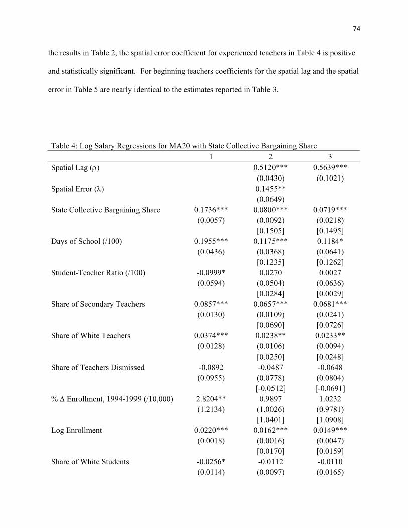
74  

 

the results in Table 2, the spatial error coefficient for experienced teachers in Table 4 is positive

and statistically significant. For beginning teachers coefficients for the spatial lag and the spatial

error in Table 5 are nearly identical to the estimates reported in Table 3.

Table 4: Log Salary Regressions for MA20 with State Collective Bargaining Share 1 2 3 Spatial Lag (ρ) 0.5120*** 0.5639***

(0.0430) (0.1021) Spatial Error (λ) 0.1455**

(0.0649) State Collective Bargaining Share 0.1736*** 0.0800*** 0.0719***

(0.0057) (0.0092) (0.0218) [0.1505] [0.1495]

Days of School (/100) 0.1955*** 0.1175*** 0.1184* (0.0436) (0.0368) (0.0641)

[0.1235] [0.1262] Student-Teacher Ratio (/100) -0.0999* 0.0270 0.0027

(0.0594) (0.0504) (0.0636) [0.0284] [0.0029]

Share of Secondary Teachers 0.0857*** 0.0657*** 0.0681*** (0.0130) (0.0109) (0.0241)

[0.0690] [0.0726] Share of White Teachers 0.0374*** 0.0238** 0.0233**

(0.0128) (0.0106) (0.0094) [0.0250] [0.0248]

Share of Teachers Dismissed -0.0892 -0.0487 -0.0648 (0.0955) (0.0778) (0.0804)

[-0.0512] [-0.0691] % Δ Enrollment, 1994-1999 (/10,000) 2.8204** 0.9897 1.0232

(1.2134) (1.0026) (0.9781) [1.0401] [1.0908]

Log Enrollment 0.0220*** 0.0162*** 0.0149*** (0.0018) (0.0016) (0.0047)

[0.0170] [0.0159] Share of White Students -0.0256* -0.0112 -0.0110

(0.0114) (0.0097) (0.0165)

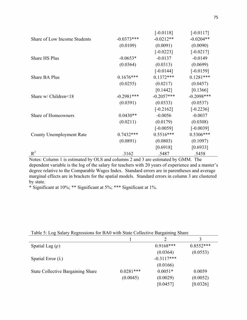
75  

 

[-0.0118] [-0.0117] Share of Low Income Students -0.0373*** -0.0212** -0.0204**

(0.0109) (0.0091) (0.0090) [-0.0223] [-0.0217]

Share HS Plus -0.0653* -0.0137 -0.0149 (0.0364) (0.0313) (0.0699)

[-0.0144] [-0.0159] Share BA Plus 0.1676*** 0.1372*** 0.1281***

(0.0255) (0.0217) (0.0457) [0.1442] [0.1366]

Share w/ Children<18 -0.2981*** -0.2057*** -0.2098*** (0.0391) (0.0333) (0.0537)

[-0.2162] [-0.2236] Share of Homeowners 0.0430** -0.0056 -0.0037

(0.0211) (0.0179) (0.0308) [-0.0059] [-0.0039]

County Unemployment Rate 0.7432*** 0.5516*** 0.5306*** (0.0891) (0.0803) (0.1097)

[0.6918] [0.6933] R2 .3162 .5487 .5458

Notes: Column 1 is estimated by OLS and columns 2 and 3 are estimated by GMM. The dependent variable is the log of the salary for teachers with 20 years of experience and a master’s degree relative to the Comparable Wages Index. Standard errors are in parentheses and average marginal effects are in brackets for the spatial models. Standard errors in column 3 are clustered by state. * Significant at 10%; ** Significant at 5%; *** Significant at 1%.

Table 5: Log Salary Regressions for BA0 with State Collective Bargaining Share 1 2 3 Spatial Lag (ρ) 0.9168*** 0.8552***

(0.0364) (0.0553) Spatial Error (λ) -0.3117***

(0.0166) State Collective Bargaining Share 0.0281*** 0.0051* 0.0059

(0.0045) (0.0029) (0.0052) [0.0457] [0.0326]

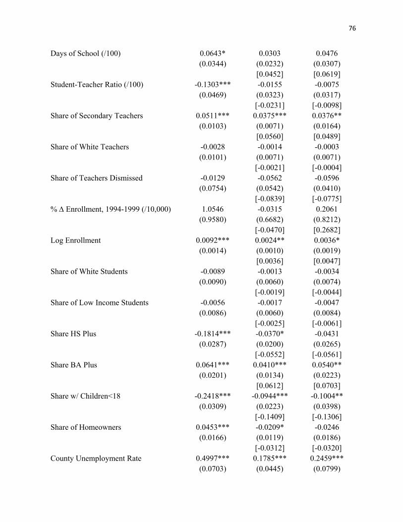
76  

 

Days of School (/100) 0.0643* 0.0303 0.0476 (0.0344) (0.0232) (0.0307)

[0.0452] [0.0619] Student-Teacher Ratio (/100) -0.1303*** -0.0155 -0.0075

(0.0469) (0.0323) (0.0317) [-0.0231] [-0.0098]

Share of Secondary Teachers 0.0511*** 0.0375*** 0.0376** (0.0103) (0.0071) (0.0164)

[0.0560] [0.0489] Share of White Teachers -0.0028 -0.0014 -0.0003

(0.0101) (0.0071) (0.0071) [-0.0021] [-0.0004]

Share of Teachers Dismissed -0.0129 -0.0562 -0.0596 (0.0754) (0.0542) (0.0410)

[-0.0839] [-0.0775] % Δ Enrollment, 1994-1999 (/10,000) 1.0546 -0.0315 0.2061

(0.9580) (0.6682) (0.8212) [-0.0470] [0.2682]

Log Enrollment 0.0092*** 0.0024** 0.0036* (0.0014) (0.0010) (0.0019)

[0.0036] [0.0047] Share of White Students -0.0089 -0.0013 -0.0034

(0.0090) (0.0060) (0.0074) [-0.0019] [-0.0044]

Share of Low Income Students -0.0056 -0.0017 -0.0047 (0.0086) (0.0060) (0.0084)

[-0.0025] [-0.0061] Share HS Plus -0.1814*** -0.0370* -0.0431

(0.0287) (0.0200) (0.0265) [-0.0552] [-0.0561]

Share BA Plus 0.0641*** 0.0410*** 0.0540** (0.0201) (0.0134) (0.0223)

[0.0612] [0.0703] Share w/ Children<18 -0.2418*** -0.0944*** -0.1004**

(0.0309) (0.0223) (0.0398) [-0.1409] [-0.1306]

Share of Homeowners 0.0453*** -0.0209* -0.0246 (0.0166) (0.0119) (0.0186)

[-0.0312] [-0.0320] County Unemployment Rate 0.4997*** 0.1785*** 0.2459***

(0.0703) (0.0445) (0.0799)

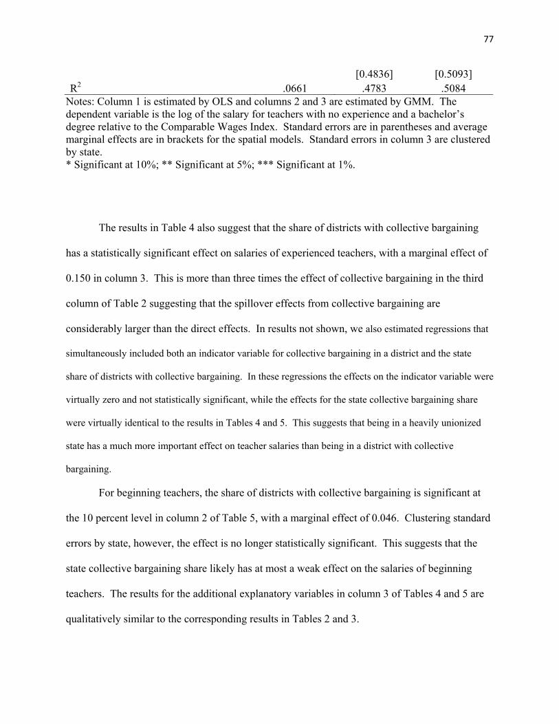
77  

 

[0.4836] [0.5093] R2 .0661 .4783 .5084

Notes: Column 1 is estimated by OLS and columns 2 and 3 are estimated by GMM. The dependent variable is the log of the salary for teachers with no experience and a bachelor’s degree relative to the Comparable Wages Index. Standard errors are in parentheses and average marginal effects are in brackets for the spatial models. Standard errors in column 3 are clustered by state. * Significant at 10%; ** Significant at 5%; *** Significant at 1%.

The results in Table 4 also suggest that the share of districts with collective bargaining

has a statistically significant effect on salaries of experienced teachers, with a marginal effect of

0.150 in column 3. This is more than three times the effect of collective bargaining in the third

column of Table 2 suggesting that the spillover effects from collective bargaining are

considerably larger than the direct effects. In results not shown, we also estimated regressions that

simultaneously included both an indicator variable for collective bargaining in a district and the state

share of districts with collective bargaining. In these regressions the effects on the indicator variable were

virtually zero and not statistically significant, while the effects for the state collective bargaining share

were virtually identical to the results in Tables 4 and 5. This suggests that being in a heavily unionized

state has a much more important effect on teacher salaries than being in a district with collective

bargaining.

For beginning teachers, the share of districts with collective bargaining is significant at

the 10 percent level in column 2 of Table 5, with a marginal effect of 0.046. Clustering standard

errors by state, however, the effect is no longer statistically significant. This suggests that the

state collective bargaining share likely has at most a weak effect on the salaries of beginning

teachers. The results for the additional explanatory variables in column 3 of Tables 4 and 5 are

qualitatively similar to the corresponding results in Tables 2 and 3.

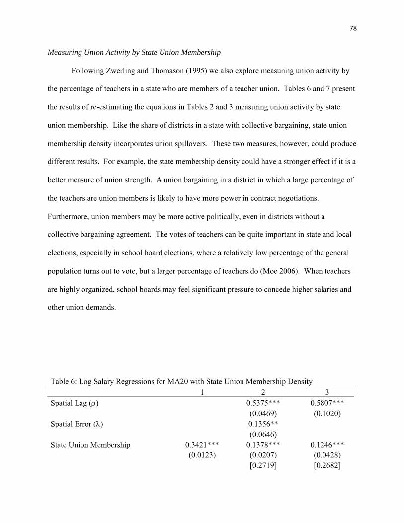
78  

 

Measuring Union Activity by State Union Membership

Following Zwerling and Thomason (1995) we also explore measuring union activity by

the percentage of teachers in a state who are members of a teacher union. Tables 6 and 7 present

the results of re-estimating the equations in Tables 2 and 3 measuring union activity by state

union membership. Like the share of districts in a state with collective bargaining, state union

membership density incorporates union spillovers. These two measures, however, could produce

different results. For example, the state membership density could have a stronger effect if it is a

better measure of union strength. A union bargaining in a district in which a large percentage of

the teachers are union members is likely to have more power in contract negotiations.

Furthermore, union members may be more active politically, even in districts without a

collective bargaining agreement. The votes of teachers can be quite important in state and local

elections, especially in school board elections, where a relatively low percentage of the general

population turns out to vote, but a larger percentage of teachers do (Moe 2006). When teachers

are highly organized, school boards may feel significant pressure to concede higher salaries and

other union demands.

Table 6: Log Salary Regressions for MA20 with State Union Membership Density 1 2 3 Spatial Lag (ρ) 0.5375*** 0.5807***

(0.0469) (0.1020) Spatial Error (λ) 0.1356**

(0.0646) State Union Membership 0.3421*** 0.1378*** 0.1246***

(0.0123) (0.0207) (0.0428) [0.2719] [0.2682]

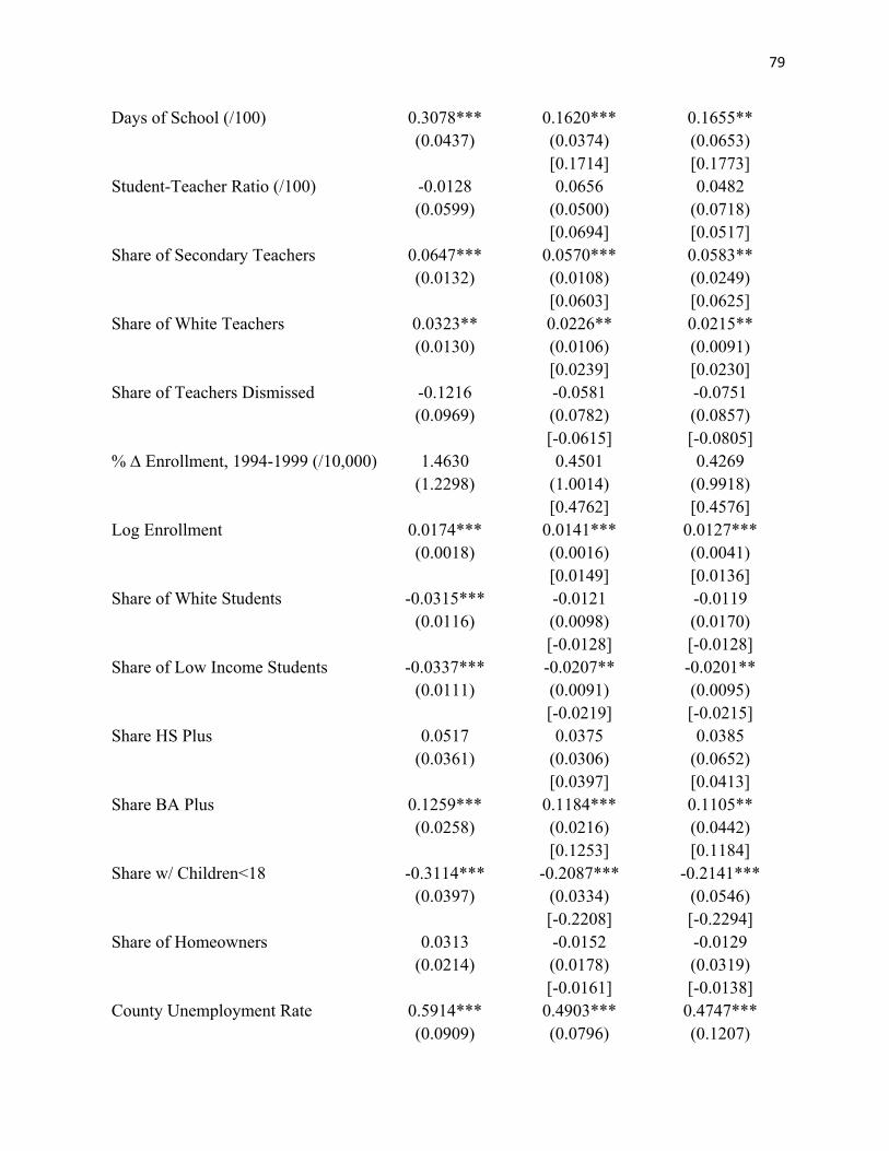
79  

 

Days of School (/100) 0.3078*** 0.1620*** 0.1655** (0.0437) (0.0374) (0.0653)

[0.1714] [0.1773] Student-Teacher Ratio (/100) -0.0128 0.0656 0.0482

(0.0599) (0.0500) (0.0718) [0.0694] [0.0517]

Share of Secondary Teachers 0.0647*** 0.0570*** 0.0583** (0.0132) (0.0108) (0.0249)

[0.0603] [0.0625] Share of White Teachers 0.0323** 0.0226** 0.0215**

(0.0130) (0.0106) (0.0091) [0.0239] [0.0230]

Share of Teachers Dismissed -0.1216 -0.0581 -0.0751 (0.0969) (0.0782) (0.0857)

[-0.0615] [-0.0805] % Δ Enrollment, 1994-1999 (/10,000) 1.4630 0.4501 0.4269

(1.2298) (1.0014) (0.9918) [0.4762] [0.4576]

Log Enrollment 0.0174*** 0.0141*** 0.0127*** (0.0018) (0.0016) (0.0041)

[0.0149] [0.0136] Share of White Students -0.0315*** -0.0121 -0.0119

(0.0116) (0.0098) (0.0170) [-0.0128] [-0.0128]

Share of Low Income Students -0.0337*** -0.0207** -0.0201** (0.0111) (0.0091) (0.0095)

[-0.0219] [-0.0215] Share HS Plus 0.0517 0.0375 0.0385

(0.0361) (0.0306) (0.0652) [0.0397] [0.0413]

Share BA Plus 0.1259*** 0.1184*** 0.1105** (0.0258) (0.0216) (0.0442)

[0.1253] [0.1184] Share w/ Children<18 -0.3114*** -0.2087*** -0.2141***

(0.0397) (0.0334) (0.0546) [-0.2208] [-0.2294]

Share of Homeowners 0.0313 -0.0152 -0.0129 (0.0214) (0.0178) (0.0319)

[-0.0161] [-0.0138] County Unemployment Rate 0.5914*** 0.4903*** 0.4747***

(0.0909) (0.0796) (0.1207)

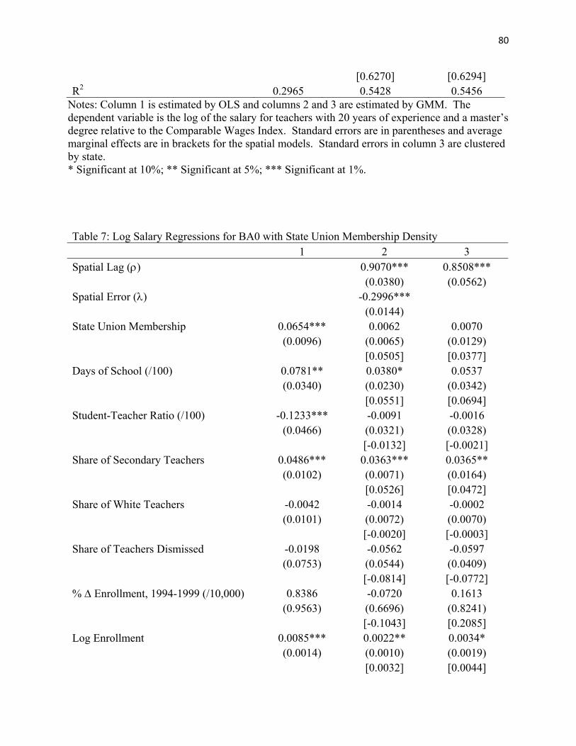
80  

 

[0.6270] [0.6294] R2 0.2965 0.5428 0.5456

Notes: Column 1 is estimated by OLS and columns 2 and 3 are estimated by GMM. The dependent variable is the log of the salary for teachers with 20 years of experience and a master’s degree relative to the Comparable Wages Index. Standard errors are in parentheses and average marginal effects are in brackets for the spatial models. Standard errors in column 3 are clustered by state. * Significant at 10%; ** Significant at 5%; *** Significant at 1%.

Table 7: Log Salary Regressions for BA0 with State Union Membership Density 1 2 3 Spatial Lag (ρ) 0.9070*** 0.8508***

(0.0380) (0.0562) Spatial Error (λ) -0.2996***

(0.0144) State Union Membership 0.0654*** 0.0062 0.0070

(0.0096) (0.0065) (0.0129) [0.0505] [0.0377]

Days of School (/100) 0.0781** 0.0380* 0.0537 (0.0340) (0.0230) (0.0342)

[0.0551] [0.0694] Student-Teacher Ratio (/100) -0.1233*** -0.0091 -0.0016

(0.0466) (0.0321) (0.0328) [-0.0132] [-0.0021]

Share of Secondary Teachers 0.0486*** 0.0363*** 0.0365** (0.0102) (0.0071) (0.0164)

[0.0526] [0.0472] Share of White Teachers -0.0042 -0.0014 -0.0002

(0.0101) (0.0072) (0.0070) [-0.0020] [-0.0003]

Share of Teachers Dismissed -0.0198 -0.0562 -0.0597 (0.0753) (0.0544) (0.0409)

[-0.0814] [-0.0772] % Δ Enrollment, 1994-1999 (/10,000) 0.8386 -0.0720 0.1613

(0.9563) (0.6696) (0.8241) [-0.1043] [0.2085]

Log Enrollment 0.0085*** 0.0022** 0.0034* (0.0014) (0.0010) (0.0019)

[0.0032] [0.0044]

81  

 

Share of White Students -0.0108 -0.0012 -0.0032 (0.0090) (0.0061) (0.0075)

[-0.0017] [-0.0041] Share of Low Income Students -0.0036 -0.0025 -0.0053

(0.0086) (0.0061) (0.0081) [-0.0036] [-0.0068]

Share HS Plus -0.1673*** -0.0320 -0.0374 (0.0281) (0.0195) (0.0278)

[-0.0464] [-0.0483] Share BA Plus 0.0573*** 0.0403*** 0.0526**

(0.0201) (0.0135) (0.0228) [0.0584] [0.0680]

Share w/ Children<18 -0.2424*** -0.0981*** -0.1023** (0.0308) (0.0225) (0.0397)

[-0.1422] [-0.1322] Share of Homeowners 0.0462*** -0.0220* -0.0260

(0.0166) (0.0121) (0.0193) [-0.0319] [-0.0336]

County Unemployment Rate 0.4655*** 0.1837*** 0.2466*** (0.0707) (0.0449) (0.0813)

[0.4706] [0.5038] R2 0.0679 0.4777 0.5060

Notes: Column 1 is estimated by OLS and columns 2 and 3 are estimated by GMM. The dependent variable is the log of the salary for teachers with no experience and a bachelor’s degree relative to the Comparable Wages Index. Standard errors are in parentheses and average marginal effects are in brackets for the spatial models. Standard errors in column 3 are clustered by state. * Significant at 10%; ** Significant at 5%; *** Significant at 1%.

The spatial lag and spatial error results in Tables 6 and 7 measuring union activity by the

state membership share are very similar to the corresponding estimates in Tables 4 and 5. The

results for the non-union variables in column 3 are quite similar to the corresponding estimates in

Tables 4 and 5 as well. For experienced teachers the state membership density has a significant

marginal effect of 0.268 in column 3 of Table 6, but the effect for beginning teachers is

insignificant. While the marginal effect for experienced teachers is larger than that in Table 4,

82  

 

we must also account for the fact that the state membership density is less dispersed than the

state collective bargaining share to assess their relative impacts. The state collective bargaining

share has a minimum value of zero, a maximum value of one, and a standard deviation of 0.410,

while the state membership density ranges between 0.312 and 0.992 and has a standard deviation

of 0.185. Therefore, according to the column 3 estimates in Tables 4 and 6 moving from a state

with no collective bargaining to a state with complete collective bargaining coverage would

increase salaries for experienced teachers by 16.1 percent, while moving from the state with the

lowest membership density to the state with the greatest membership density would increase

salaries for experienced teachers by 20.9 percent. Alternatively, moving from one standard deviation

below the mean to one standard deviation above the mean of union activity increases salaries for

experienced teachers by 13.2 percent for the collective bargaining share but only by 11.4 percent for the

state membership density. Moving from the 25th percentile to the 75th percentile of union activity

increases salaries for experienced teachers by 14.1 percent for the collective bargaining share and by 9.3

percent for the state membership density. Thus, although the two measures differ, their estimated

impacts on the salaries of experienced teachers are both fairly large.

6. Conclusion

Using a national level dataset this paper has shown that salaries for both experienced and

beginning teachers are considerably affected by teacher salaries in nearby districts, though the

effect is larger for beginning teachers. Investigations of the determinants of teacher salaries that

ignore spatial dependence are likely to be misspecified. The results of the spatial regressions

suggest that a number of other important factors affect teacher salaries. The effect of unions on

teacher salaries is given considerable attention in this paper. Accounting for union spillovers, we

find that collective bargaining and union membership density in a state increase salaries for

83  

 

experienced teachers by as much as 16 and 21 percent, respectively, but the estimated effects on

the salaries of beginning teachers are much smaller. Given the relatively weak bargaining

position of beginning relative to experienced teachers within unions (i.e. potential members

versus voting members), this result is not surprising. Although the median voter model

explanation for this pattern of union wage effects appears most persuasive, we cannot rule out

the possibility that wage-depressing monopsony effects among experienced teachers are being

offset in union but not nonunion districts.

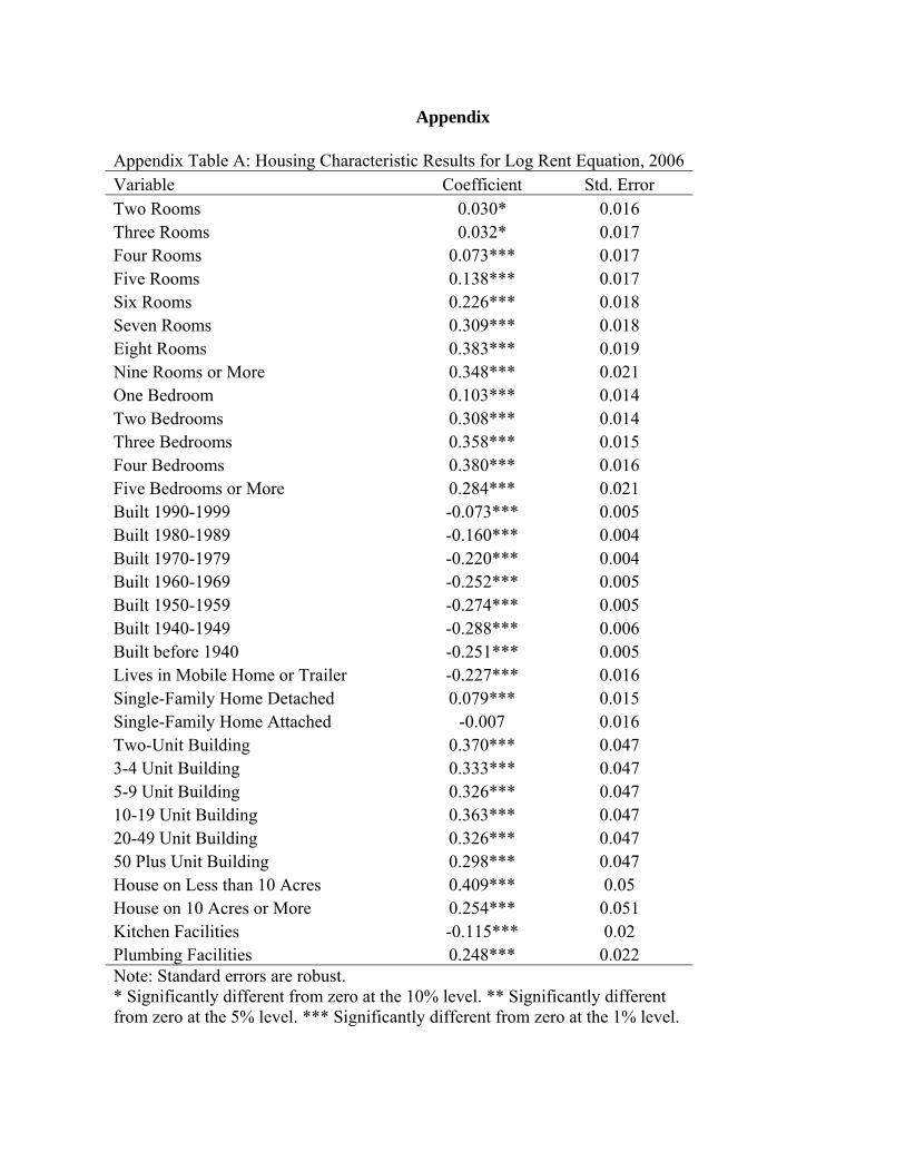
Appendix

Appendix Table A: Housing Characteristic Results for Log Rent Equation, 2006 Variable Coefficient Std. Error Two Rooms 0.030* 0.016 Three Rooms 0.032* 0.017 Four Rooms 0.073*** 0.017 Five Rooms 0.138*** 0.017 Six Rooms 0.226*** 0.018 Seven Rooms 0.309*** 0.018 Eight Rooms 0.383*** 0.019 Nine Rooms or More 0.348*** 0.021 One Bedroom 0.103*** 0.014 Two Bedrooms 0.308*** 0.014 Three Bedrooms 0.358*** 0.015 Four Bedrooms 0.380*** 0.016 Five Bedrooms or More 0.284*** 0.021 Built 1990-1999 -0.073*** 0.005 Built 1980-1989 -0.160*** 0.004 Built 1970-1979 -0.220*** 0.004 Built 1960-1969 -0.252*** 0.005 Built 1950-1959 -0.274*** 0.005 Built 1940-1949 -0.288*** 0.006 Built before 1940 -0.251*** 0.005 Lives in Mobile Home or Trailer -0.227*** 0.016 Single-Family Home Detached 0.079*** 0.015 Single-Family Home Attached -0.007 0.016 Two-Unit Building 0.370*** 0.047 3-4 Unit Building 0.333*** 0.047 5-9 Unit Building 0.326*** 0.047 10-19 Unit Building 0.363*** 0.047 20-49 Unit Building 0.326*** 0.047 50 Plus Unit Building 0.298*** 0.047 House on Less than 10 Acres 0.409*** 0.05 House on 10 Acres or More 0.254*** 0.051 Kitchen Facilities -0.115*** 0.02 Plumbing Facilities 0.248*** 0.022 Note: Standard errors are robust. * Significantly different from zero at the 10% level. ** Significantly different from zero at the 5% level. *** Significantly different from zero at the 1% level.

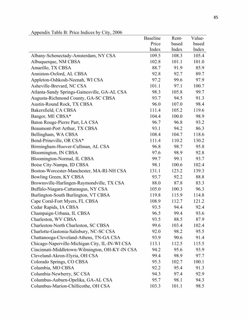
85  

 

Appendix Table B: Price Indices by City, 2006

Baseline Price Index

Rent-based Index

Value-based Index

Albany-Schenectady-Amsterdam, NY CSA 109.5 108.3 105.4Albuquerque, NM CBSA 102.8 101.1 101.0Amarillo, TX CBSA 88.7 91.9 85.9Anniston-Oxford, AL CBSA 92.8 92.7 89.7Appleton-Oshkosh-Neenah, WI CSA 97.2 99.6 97.9Asheville-Brevard, NC CSA 101.1 97.1 100.7Atlanta-Sandy Springs-Gainesville, GA-AL CSA 98.3 105.8 99.7Augusta-Richmond County, GA-SC CBSA 93.7 94.5 91.3Austin-Round Rock, TX CBSA 96.0 107.0 98.4Bakersfield, CA CBSA 111.4 105.2 119.6Bangor, ME CBSA* 104.4 100.0 98.9Baton Rouge-Pierre Part, LA CSA 96.7 96.8 93.2Beaumont-Port Arthur, TX CBSA 93.1 94.2 86.3Bellingham, WA CBSA 108.4 104.7 118.6Bend-Prineville, OR CSA* 111.4 110.2 130.2Birmingham-Hoover-Cullman, AL CSA 96.8 98.7 95.8Bloomington, IN CBSA 97.6 98.9 92.8Bloomington-Normal, IL CBSA 99.7 99.1 93.7Boise City-Nampa, ID CBSA 98.1 100.6 102.4Boston-Worcester-Manchester, MA-RI-NH CSA 131.1 123.2 139.3Bowling Green, KY CBSA 93.7 92.2 88.8Brownsville-Harlingen-Raymondville, TX CSA 88.0 87.8 83.3Buffalo-Niagara-Cattaraugus, NY CSA 105.0 100.3 96.3Burlington-South Burlington, VT CBSA 119.8 115.9 114.8Cape Coral-Fort Myers, FL CBSA 108.9 112.7 121.2Cedar Rapids, IA CBSA 93.5 94.4 92.4Champaign-Urbana, IL CBSA 96.5 99.4 93.6Charleston, WV CBSA 93.5 88.5 87.9Charleston-North Charleston, SC CBSA 99.6 103.4 102.4Charlotte-Gastonia-Salisbury, NC-SC CSA 92.0 98.2 95.5Chattanooga-Cleveland-Athens, TN-GA CSA 93.9 90.6 91.4Chicago-Naperville-Michigan City, IL-IN-WI CSA 113.1 112.5 115.5Cincinnati-Middletown-Wilmington, OH-KY-IN CSA 94.2 95.6 93.9Cleveland-Akron-Elyria, OH CSA 99.4 98.9 97.7Colorado Springs, CO CBSA 95.3 102.7 100.1Columbia, MO CBSA 92.2 95.4 91.3Columbia-Newberry, SC CSA 94.3 97.4 92.9Columbus-Auburn-Opelika, GA-AL CSA 95.7 98.1 94.3Columbus-Marion-Chillicothe, OH CSA 103.3 101.1 98.5

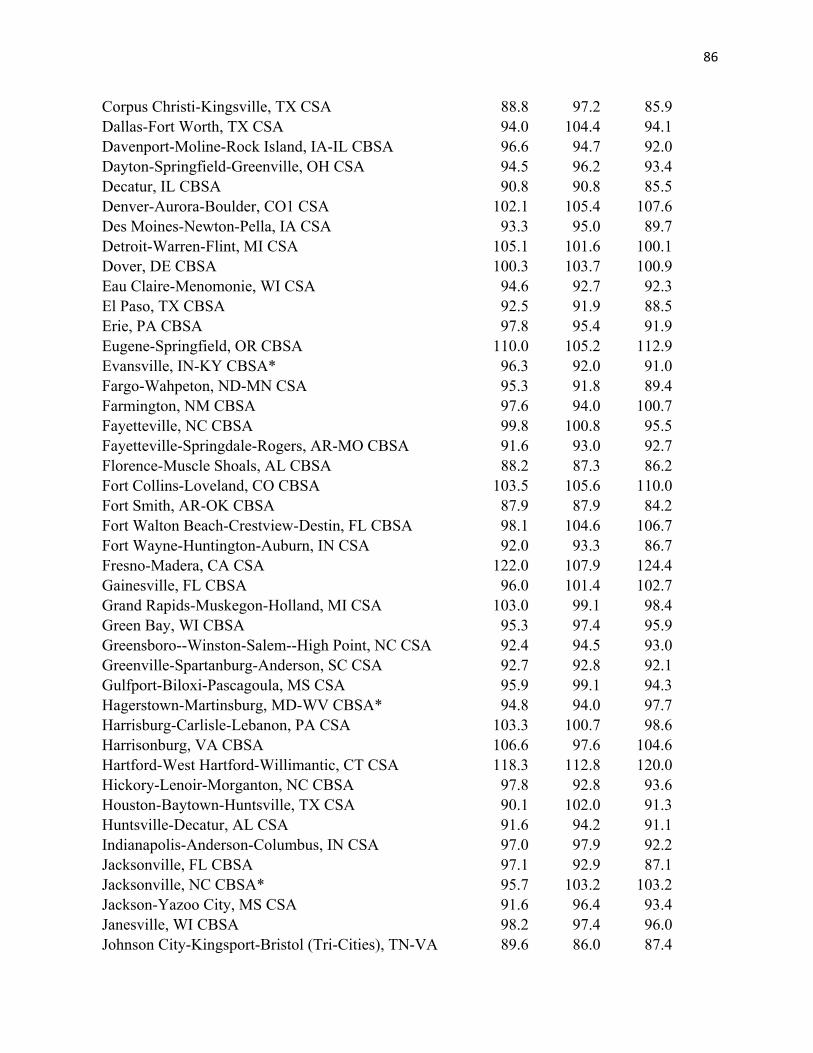
86  

 

Corpus Christi-Kingsville, TX CSA 88.8 97.2 85.9Dallas-Fort Worth, TX CSA 94.0 104.4 94.1Davenport-Moline-Rock Island, IA-IL CBSA 96.6 94.7 92.0Dayton-Springfield-Greenville, OH CSA 94.5 96.2 93.4Decatur, IL CBSA 90.8 90.8 85.5Denver-Aurora-Boulder, CO1 CSA 102.1 105.4 107.6Des Moines-Newton-Pella, IA CSA 93.3 95.0 89.7Detroit-Warren-Flint, MI CSA 105.1 101.6 100.1Dover, DE CBSA 100.3 103.7 100.9Eau Claire-Menomonie, WI CSA 94.6 92.7 92.3El Paso, TX CBSA 92.5 91.9 88.5Erie, PA CBSA 97.8 95.4 91.9Eugene-Springfield, OR CBSA 110.0 105.2 112.9Evansville, IN-KY CBSA* 96.3 92.0 91.0Fargo-Wahpeton, ND-MN CSA 95.3 91.8 89.4Farmington, NM CBSA 97.6 94.0 100.7Fayetteville, NC CBSA 99.8 100.8 95.5Fayetteville-Springdale-Rogers, AR-MO CBSA 91.6 93.0 92.7Florence-Muscle Shoals, AL CBSA 88.2 87.3 86.2Fort Collins-Loveland, CO CBSA 103.5 105.6 110.0Fort Smith, AR-OK CBSA 87.9 87.9 84.2Fort Walton Beach-Crestview-Destin, FL CBSA 98.1 104.6 106.7Fort Wayne-Huntington-Auburn, IN CSA 92.0 93.3 86.7Fresno-Madera, CA CSA 122.0 107.9 124.4Gainesville, FL CBSA 96.0 101.4 102.7Grand Rapids-Muskegon-Holland, MI CSA 103.0 99.1 98.4Green Bay, WI CBSA 95.3 97.4 95.9Greensboro--Winston-Salem--High Point, NC CSA 92.4 94.5 93.0Greenville-Spartanburg-Anderson, SC CSA 92.7 92.8 92.1Gulfport-Biloxi-Pascagoula, MS CSA 95.9 99.1 94.3Hagerstown-Martinsburg, MD-WV CBSA* 94.8 94.0 97.7Harrisburg-Carlisle-Lebanon, PA CSA 103.3 100.7 98.6Harrisonburg, VA CBSA 106.6 97.6 104.6Hartford-West Hartford-Willimantic, CT CSA 118.3 112.8 120.0Hickory-Lenoir-Morganton, NC CBSA 97.8 92.8 93.6Houston-Baytown-Huntsville, TX CSA 90.1 102.0 91.3Huntsville-Decatur, AL CSA 91.6 94.2 91.1Indianapolis-Anderson-Columbus, IN CSA 97.0 97.9 92.2Jacksonville, FL CBSA 97.1 92.9 87.1Jacksonville, NC CBSA* 95.7 103.2 103.2Jackson-Yazoo City, MS CSA 91.6 96.4 93.4Janesville, WI CBSA 98.2 97.4 96.0Johnson City-Kingsport-Bristol (Tri-Cities), TN-VA 89.6 86.0 87.4

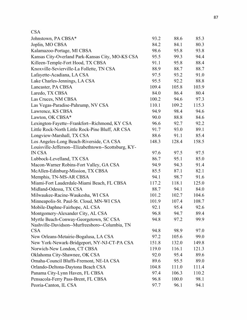
87  

 

CSA Johnstown, PA CBSA* 93.2 88.6 85.3Joplin, MO CBSA 84.2 84.1 80.3Kalamazoo-Portage, MI CBSA 98.6 95.8 93.8Kansas City-Overland Park-Kansas City, MO-KS CSA 95.5 99.3 94.4Killeen-Temple-Fort Hood, TX CBSA 91.1 95.8 88.4Knoxville-Sevierville-La Follette, TN CSA 88.9 88.7 88.7Lafayette-Acadiana, LA CSA 97.5 93.2 91.0Lake Charles-Jennings, LA CSA 95.5 92.2 88.8Lancaster, PA CBSA 109.4 105.8 103.9Laredo, TX CBSA 84.0 86.4 80.4Las Cruces, NM CBSA 100.2 94.6 97.3Las Vegas-Paradise-Pahrump, NV CSA 110.1 109.2 115.3Lawrence, KS CBSA 94.9 98.4 94.6Lawton, OK CBSA* 90.0 88.8 84.6Lexington-Fayette--Frankfort--Richmond, KY CSA 96.6 92.7 92.2Little Rock-North Little Rock-Pine Bluff, AR CSA 91.7 93.0 89.1Longview-Marshall, TX CSA 88.6 91.1 85.4Los Angeles-Long Beach-Riverside, CA CSA 148.3 128.4 158.5Louisville-Jefferson--Elizabethtown--Scottsburg, KY-IN CSA 97.6 97.5 97.5Lubbock-Levelland, TX CSA 86.7 95.1 85.0Macon-Warner Robins-Fort Valley, GA CSA 94.9 94.3 91.4McAllen-Edinburg-Mission, TX CBSA 85.5 87.1 82.1Memphis, TN-MS-AR CBSA 94.1 98.7 91.6Miami-Fort Lauderdale-Miami Beach, FL CBSA 117.2 118.1 125.0Midland-Odessa, TX CSA 88.7 94.1 84.0Milwaukee-Racine-Waukesha, WI CSA 101.2 102.7 104.6Minneapolis-St. Paul-St. Cloud, MN-WI CSA 101.9 107.4 108.7Mobile-Daphne-Fairhope, AL CSA 92.1 95.4 92.6Montgomery-Alexander City, AL CSA 96.8 94.7 89.4Myrtle Beach-Conway-Georgetown, SC CSA 94.8 97.2 99.9Nashville-Davidson--Murfreesboro--Columbia, TN CSA 94.8 98.9 97.0New Orleans-Metairie-Bogalusa, LA CSA 97.2 105.6 99.0New York-Newark-Bridgeport, NY-NJ-CT-PA CSA 151.8 132.0 149.8Norwich-New London, CT CBSA 119.0 116.1 121.3Oklahoma City-Shawnee, OK CSA 92.0 95.4 89.6Omaha-Council Bluffs-Fremont, NE-IA CSA 89.6 95.5 89.0Orlando-Deltona-Daytona Beach CSA 104.8 111.0 111.4Panama City-Lynn Haven, FL CBSA 97.4 106.3 110.2Pensacola-Ferry Pass-Brent, FL CBSA 96.8 100.0 98.1Peoria-Canton, IL CSA 97.7 96.1 94.1

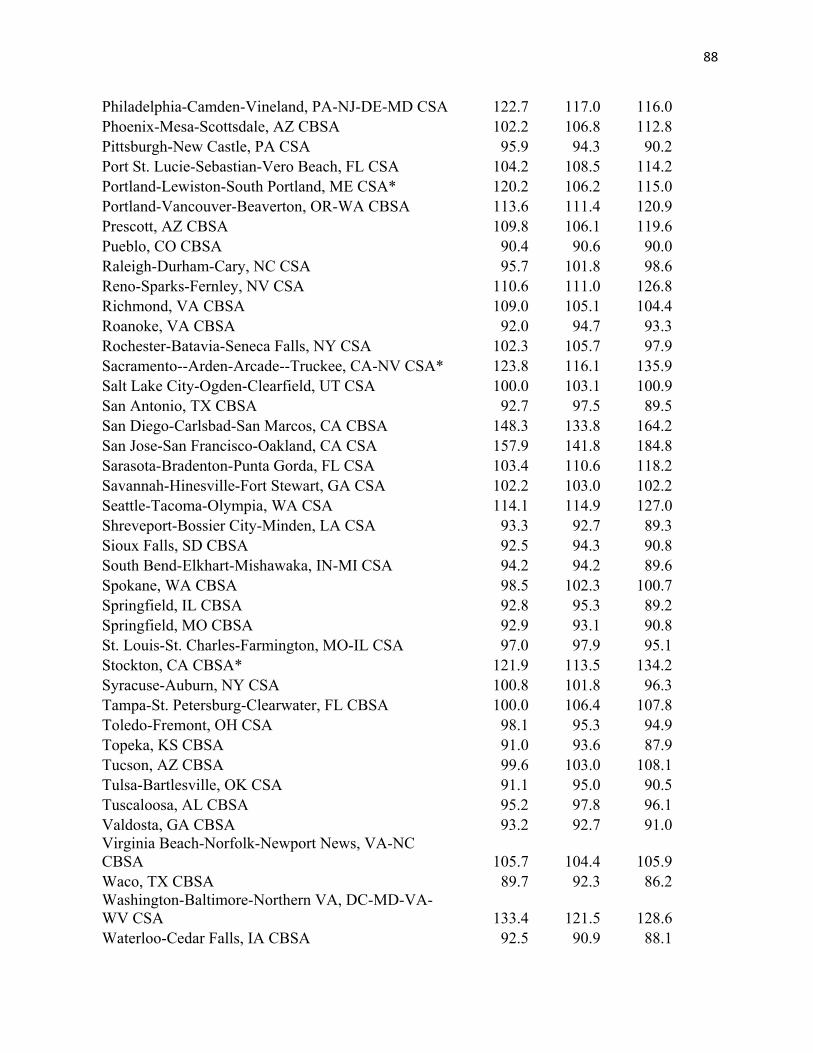
88  

 

Philadelphia-Camden-Vineland, PA-NJ-DE-MD CSA 122.7 117.0 116.0Phoenix-Mesa-Scottsdale, AZ CBSA 102.2 106.8 112.8Pittsburgh-New Castle, PA CSA 95.9 94.3 90.2Port St. Lucie-Sebastian-Vero Beach, FL CSA 104.2 108.5 114.2Portland-Lewiston-South Portland, ME CSA* 120.2 106.2 115.0Portland-Vancouver-Beaverton, OR-WA CBSA 113.6 111.4 120.9Prescott, AZ CBSA 109.8 106.1 119.6Pueblo, CO CBSA 90.4 90.6 90.0Raleigh-Durham-Cary, NC CSA 95.7 101.8 98.6Reno-Sparks-Fernley, NV CSA 110.6 111.0 126.8Richmond, VA CBSA 109.0 105.1 104.4Roanoke, VA CBSA 92.0 94.7 93.3Rochester-Batavia-Seneca Falls, NY CSA 102.3 105.7 97.9Sacramento--Arden-Arcade--Truckee, CA-NV CSA* 123.8 116.1 135.9Salt Lake City-Ogden-Clearfield, UT CSA 100.0 103.1 100.9San Antonio, TX CBSA 92.7 97.5 89.5San Diego-Carlsbad-San Marcos, CA CBSA 148.3 133.8 164.2San Jose-San Francisco-Oakland, CA CSA 157.9 141.8 184.8Sarasota-Bradenton-Punta Gorda, FL CSA 103.4 110.6 118.2Savannah-Hinesville-Fort Stewart, GA CSA 102.2 103.0 102.2Seattle-Tacoma-Olympia, WA CSA 114.1 114.9 127.0Shreveport-Bossier City-Minden, LA CSA 93.3 92.7 89.3Sioux Falls, SD CBSA 92.5 94.3 90.8South Bend-Elkhart-Mishawaka, IN-MI CSA 94.2 94.2 89.6Spokane, WA CBSA 98.5 102.3 100.7Springfield, IL CBSA 92.8 95.3 89.2Springfield, MO CBSA 92.9 93.1 90.8St. Louis-St. Charles-Farmington, MO-IL CSA 97.0 97.9 95.1Stockton, CA CBSA* 121.9 113.5 134.2Syracuse-Auburn, NY CSA 100.8 101.8 96.3Tampa-St. Petersburg-Clearwater, FL CBSA 100.0 106.4 107.8Toledo-Fremont, OH CSA 98.1 95.3 94.9Topeka, KS CBSA 91.0 93.6 87.9Tucson, AZ CBSA 99.6 103.0 108.1Tulsa-Bartlesville, OK CSA 91.1 95.0 90.5Tuscaloosa, AL CBSA 95.2 97.8 96.1Valdosta, GA CBSA 93.2 92.7 91.0Virginia Beach-Norfolk-Newport News, VA-NC CBSA 105.7 104.4 105.9Waco, TX CBSA 89.7 92.3 86.2Washington-Baltimore-Northern VA, DC-MD-VA-WV CSA 133.4 121.5 128.6Waterloo-Cedar Falls, IA CBSA 92.5 90.9 88.1

89  

 

Wausau-Merrill, WI CSA 94.0 94.7 91.0Wichita-Winfield, KS CSA 94.9 94.7 88.4York-Hanover-Gettysburg, PA CSA 101.5 97.9 98.0Youngstown-Warren-East Liverpool, OH-PA CSA 94.4 89.9 88.6

*Indicates ACCRA data are not available for 2005.

90  

 

Appendix Table C: Variables and Data Sources Variable Data Source Log Wage Current Population Survey Worker Characteristics Current Population Survey Baseline Price Index ACCRA Rent-based Modified Price Index American Community Survey & ACCRA Housing Value-based Modified Price Index American Community Survey & ACCRA Quality-Adjusted Gross Rents American Community Survey Quality-Adjusted Housing Values American Community Survey Non-housing Prices ACCRA Gulf Coast Consulted Map Atlantic Coast Consulted Map Pacific Coast Consulted Map January Temperature ERS Natural Amenities Scale July Temperature ERS Natural Amenities Scale January Sun ERS Natural Amenities Scale July Humidity ERS Natural Amenities Scale % Water Area ERS Natural Amenities Scale Topography 2 ERS Natural Amenities Scale Topography 3 ERS Natural Amenities Scale Topography 4 ERS Natural Amenities Scale Topography 5 ERS Natural Amenities Scale Precipitation Cities Ranked and Rated Snow Cities Ranked and Rated Violent Crime USA Counties Website Property Crime USA Counties Website Mean Commute Time American Community Survey Ozone EPA AirData Database Particulate Matter (2.5) EPA AirData Database Census Division Indicators Assigned According to Census Geography City Size Indicators Population Estimates according to Census Bureau

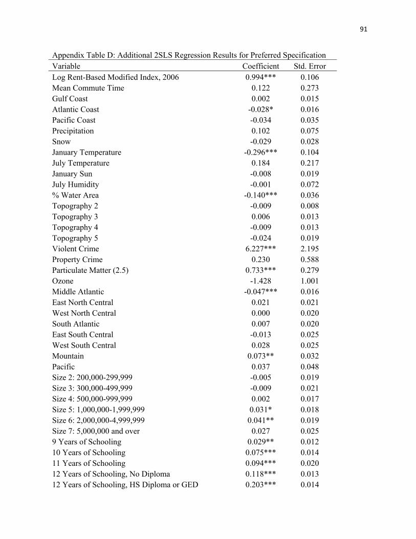
91  

 

Appendix Table D: Additional 2SLS Regression Results for Preferred Specification Variable Coefficient Std. Error Log Rent-Based Modified Index, 2006 0.994*** 0.106 Mean Commute Time 0.122 0.273 Gulf Coast 0.002 0.015 Atlantic Coast -0.028* 0.016 Pacific Coast -0.034 0.035 Precipitation 0.102 0.075 Snow -0.029 0.028 January Temperature -0.296*** 0.104 July Temperature 0.184 0.217 January Sun -0.008 0.019 July Humidity -0.001 0.072 % Water Area -0.140*** 0.036 Topography 2 -0.009 0.008 Topography 3 0.006 0.013 Topography 4 -0.009 0.013 Topography 5 -0.024 0.019 Violent Crime 6.227*** 2.195 Property Crime 0.230 0.588 Particulate Matter (2.5) 0.733*** 0.279 Ozone -1.428 1.001 Middle Atlantic -0.047*** 0.016 East North Central 0.021 0.021 West North Central 0.000 0.020 South Atlantic 0.007 0.020 East South Central -0.013 0.025 West South Central 0.028 0.025 Mountain 0.073** 0.032 Pacific 0.037 0.048 Size 2: 200,000-299,999 -0.005 0.019 Size 3: 300,000-499,999 -0.009 0.021 Size 4: 500,000-999,999 0.002 0.017 Size 5: 1,000,000-1,999,999 0.031* 0.018 Size 6: 2,000,000-4,999,999 0.041** 0.019 Size 7: 5,000,000 and over 0.027 0.025 9 Years of Schooling 0.029** 0.012 10 Years of Schooling 0.075*** 0.014 11 Years of Schooling 0.094*** 0.020 12 Years of Schooling, No Diploma 0.118*** 0.013 12 Years of Schooling, HS Diploma or GED 0.203*** 0.014

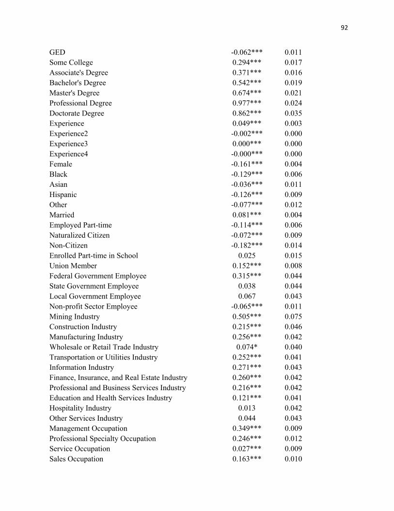
92  

 

GED -0.062*** 0.011 Some College 0.294*** 0.017 Associate's Degree 0.371*** 0.016 Bachelor's Degree 0.542*** 0.019 Master's Degree 0.674*** 0.021 Professional Degree 0.977*** 0.024 Doctorate Degree 0.862*** 0.035 Experience 0.049*** 0.003 Experience2 -0.002*** 0.000 Experience3 0.000*** 0.000 Experience4 -0.000*** 0.000 Female -0.161*** 0.004 Black -0.129*** 0.006 Asian -0.036*** 0.011 Hispanic -0.126*** 0.009 Other -0.077*** 0.012 Married 0.081*** 0.004 Employed Part-time -0.114*** 0.006 Naturalized Citizen -0.072*** 0.009 Non-Citizen -0.182*** 0.014 Enrolled Part-time in School 0.025 0.015 Union Member 0.152*** 0.008 Federal Government Employee 0.315*** 0.044 State Government Employee 0.038 0.044 Local Government Employee 0.067 0.043 Non-profit Sector Employee -0.065*** 0.011 Mining Industry 0.505*** 0.075 Construction Industry 0.215*** 0.046 Manufacturing Industry 0.256*** 0.042 Wholesale or Retail Trade Industry 0.074* 0.040 Transportation or Utilities Industry 0.252*** 0.041 Information Industry 0.271*** 0.043 Finance, Insurance, and Real Estate Industry 0.260*** 0.042 Professional and Business Services Industry 0.216*** 0.042 Education and Health Services Industry 0.121*** 0.041 Hospitality Industry 0.013 0.042 Other Services Industry 0.044 0.043 Management Occupation 0.349*** 0.009 Professional Specialty Occupation 0.246*** 0.012 Service Occupation 0.027*** 0.009 Sales Occupation 0.163*** 0.010

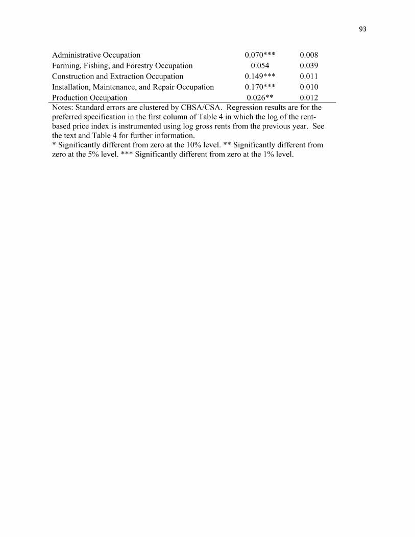
93  

 

Administrative Occupation 0.070*** 0.008 Farming, Fishing, and Forestry Occupation 0.054 0.039 Construction and Extraction Occupation 0.149*** 0.011 Installation, Maintenance, and Repair Occupation 0.170*** 0.010 Production Occupation 0.026** 0.012 Notes: Standard errors are clustered by CBSA/CSA. Regression results are for the preferred specification in the first column of Table 4 in which the log of the rent-based price index is instrumented using log gross rents from the previous year. See the text and Table 4 for further information. * Significantly different from zero at the 10% level. ** Significantly different from zero at the 5% level. *** Significantly different from zero at the 1% level.

94  

 

References Albouy, David. “The Unequal Geographic Burden of Federal Taxation.” University of Michigan

Working Paper (2008a). Albouy, David. “Are Big Cities Really Bad Places to Live? Improving Quality-of-Life Estimates

across Cities.” University of Michigan Working Paper (2008b). Anselin, Luc. Spatial Econometrics: Methods and Models. Dordrecht: Kluwer Academic

Publishers, 1988. Babcock, Linda C. and John B. Engberg. "Bargaining Unit Composition and the Returns to

Education and Tenure." Industrial & Labor Relations Review 52, no. 2 (1999): 163. Babcock, Linda C., John B. Engberg, and Robert T. Greenbaum. Wage Spillovers in Public

Sector Contract Negotiations: The Importance of Social Comparisons." Regional Science and Urban Economics 35, no. 4 (2005): 395.

Ballou, Dale, and Michael Podgursky. "Returns to Seniority among Public School Teachers."

Journal of Human Resources 37, no. 4 (2002): 892. Baugh, William H. and Joe A. Stone. "Teachers, Unions, and Wages in the 1970s: Unionism

Now Pays." Industrial & Labor Relations Review 35, no. 3 (1982): 368. Beeson, Patricia E. and Randall W. Eberts. “Identifying Productivity and Amenity Effects in

Interurban Wage Differentials.” The Review of Economics and Statistics 71, no. 3 (1989): 443.

Bellante, Don. “The North-South Differential and the Migration of Heterogeneous Labor.”

American Economic Review 69, no. 1 (1979): 166. Benhabib, Jess, Richard Rogerson, and Randall Wright. “Homework in Macroeconomics:

Household Production and Aggregate Fluctuations.” Journal of Political Economy 99, no. 6 (1991): 1166.

Bollinger, Christopher R. and Barry T. Hirsch. “Match Bias from Earnings Imputation in the

Current Population Survey: The Case of Imperfect Matching.” Journal of Labor Economics 24, no. 3 (2006): 483.

Bucks, Brian and Karen Pence. “Do Homeowners Know Their House Values and Mortgage

Terms?” Federal Reserve Board of Governors Working Paper (2006). Case, Karl E. and Robert J. Schiller. “Is There a Bubble in the Housing Market?” Brookings

Papers on Economic Activity, No. 2 (2003): 299.

95  

 

Chambers, Jay G. “The Impact of Collective Bargaining for Teachers on Resource Allocation in Public School Districts.” Journal of Urban Economics 4, no. 3 (1977): 324.

Clark, Todd E. “Rents and Prices of Housing across Areas of the United States: A Cross-Section

Examination of the Present Value Model.” Regional Science and Urban Economics 25, no. 2 (1995): 237.

Clotfelter, Charles, Elizabeth Glennie, Helen Ladd, and Jacob Vigdor. “Would Higher Salaries

Keep Teachers in High-Poverty Schools? Evidence from a Policy Intervention in North Carolina.” Journal of Public Economics 92, no. 5-6 (2008): 1352.

Coelho, Philip R.P. and Moheb A. Ghali. “The End of the North-South Wage Differential.”

American Economic Review 61, no. 5 (1971): 932. Coelho, Philip R.P. and Moheb A. Ghali. “The End of the North-South Wage Differential:

Reply.” American Economic Review 63, no. 4 (1973): 757. Davis, Morris A., Andreas Lehnert, and Robert F. Martin. “The Rent-Price Ratio for the

Aggregate Stock of Owner-Occupied Housing.” Review of Income and Wealth 54, no. 2 (2008): 279.

Davis, Morris A. and Francois Ortalo-Magné. “Household Expenditures, Wages, Rents.”

University of Wisconsin-Madison Working Paper (2008). Delaney, John Thomas. “Unionism, Bargaining Spillovers, and Teacher Compensation.” In

Advances in Industrial Relations, Vol. 2, ed. David B. Lipsky. Greenwich, CT: JAI Press, 1985: 111.

Dickie, Mark and Shelby Gerking. “Interregional Wage Differentials: An Equilibrium

Perspective.” Journal of Regional Science 27, no. 4 (1987): 571. Dickie, Mark and Shelby Gerking. “Interregional Wage Differentials in the United States: A

Survey,” in Migration and Labor Market Adjustment, eds. Jouke Van Dijk, Hendrik Folmer, Henry W. Herzog, Jr., and Alan M. Schlottmann. Dordrecht, Netherlands: Kluwer Academic, 1989: 111.

DuMond, J. Michael, Barry T. Hirsch, and David A. Macpherson. “Wage Differentials across

Labor Markets and Workers: Does Cost of Living Matter?” Economic Inquiry 37, no. 4 (1999): 577.

Ehrenberg, Ronald G. and Joshua L. Schwarz. “Public Sector Labor Markets.” In Handbook of

Labor Economics, Vol. 2, ed. Orley C. Ashenfelter and Richard Layard. Amsterdam: North Holland, 1986: 1219.

96  

 

Farber, Stephen C. and Robert J. Newman. “Accounting for South/Non-South Real Wage Differentials and for Changes in Those Differentials over Time.” The Review of Economics and Statistics 69, no. 2 (1987): 215.

Figlio, David N. “Teacher Salaries and Teacher Quality.” Economic Letters 55, no. 2 (1997):

267. Figlio, David N. “Can Public Schools Buy Better Qualified Teachers.” Industrial and Labor

Relations Review 55, no. 4 (2002): 686. Freeman, Richard. B. "Unionism Comes to the Public Sector." Journal of Economic Literature

24, no. 1 (1986): 41. Gabriel, Stuart A., Joe P. Mattey, and William L. Wascher. “Compensating Differentials and

Evolution in the Quality of Life among U.S. States.” Regional Science and Urban Economics 33, no. 5 (2003): 619.

Gerking, Shelby D. and William N. Weirick. “Compensating Differences and Interregional

Wage Differences.” The Review of Economics and Statistics 65, no. 3 (1983): 483. Glaeser, Edward L., Joseph Gyourko, and Albert Saiz. “Housing Supply and Housing Bubbles.”

Journal of Urban Economics 64, no. 2 (2008): 198. Glaeser, Edward L. and David Maré. “Cities and Skills.” Journal of Labor Economics 19, no. 2

(2001): 316. Glaeser, Edward L. and Kristina Tobio. “The Rise of the Sunbelt.” Southern Economic Journal

74, no. 3 (2008): 610. Greenbaum, Robert T. “A Spatial Study of Teachers’ Salaries in Pennsylvania School Districts.”

Journal of Labor Research 23, no. 1 (2002): 69. Greenwood, Michael J., Gary L. Hunt, Dan S. Rickman, and George I. Treyz. “Migration,

Regional Equilibrium, and the Estimation of Compensating Differentials.” American Economic Review 81, no. 5 (1991): 1382.

Gyourko, Joseph, Matthew Kahn, and Joseph Tracy. “Quality of Life and Environmental

Comparisons.” in Handbook of Regional and Urban Economics, Volume 3, eds. Paul Cheshire and Edwin S. Mills. Amsterdam: North Holland, 1999: 1413.

Henderson, J. Vernon. “Evaluating Consumer Amenities and Interregional Welfare Differences.”

Journal of Urban Economics 11, no. 1 (1982): 32. Hirsch, Barry and Edward Schumacher. “Match Bias in Wage Gap Estimates Due to Earnings

Imputation.” Journal of Labor Economics 22, no. 3 (2004): 689.

97  

 

Holmes, Alexander B. "Effects of Union Activity on Teachers' Earnings." Industrial Relations 15, no. 3 (1976): 328.

Hoxby, Caroline. M. "How Teachers’ Unions Affect Education Production." Quarterly Journal

of Economics 111, no. 3 (1996): 671. Johnson, George E. “Intermetropolitan Wage Differentials in the United States.” in The

Measurement of Labor Cost, ed. Jack Triplett. Chicago and London: University of Chicago Press, 1983: 217.

Kalenkoski, Charlene M. and Donald J. Lacombe. “Effects of Minimum Wages on Youth

Employment: The Importance of Accounting for Spatial Correlation.” Journal of Labor Research 29, no. 4 (2008): 303.

Kelejian, Harry H. and Ingmar R. Prucha. “A Generalized Spatial Two-Stage Least Squares

Procedure for Estimating a Spatial Autoregressive Model with Autoregressive Disturbances.” Journal of Real Estate Finance and Economics 17, no. 1 (1998): 99.

Kim, Chong Won, Tim T. Phipps, and Luc Anselin. “Measuring the Benefits of Air Quality

Improvement: A Spatial Hedonic Approach.” Journal of Environmental Economics and Management 45, no. 1 (2003): 24.

Koo, Jahyeong, Keith R. Phillips, and Fiona D. Sigalla. “Measuring Regional Cost of Living.”

Journal of Business & Economic Statistics 18, no. 1 (2000): 127. Krupka, Douglas J. “City Air or City Markets: Productivity Gains in Urban Areas.” IZA

Working Paper No. 3230, (2007). Lentz, Corliss. “Why Some Communities Pay More than Others? The Example of Illinois

Teachers.” Public Administration Review 58, no. 2 (1998): 137. LeSage, James P. The Theory and Practice of Spatial Econometrics. Unpublished Manuscript,

1999. Lipsky, David B. "The Effect of Collective Bargaining on Teacher Pay: A Review of the

Evidence." Educational Administration Quarterly 18, no. 1 (1982): 14. Lovenheim, Michael F. “The Effect of Teachers’ Unions on Education Production: Evidence

from Union Election Certifications in Three Midwestern States.” Stanford University Working Paper (2008).

Martin, Stephanie. “Are Public School Teacher Salaries Paid Compensating Wage Differentials

for Student Racial and Ethnic Characteristics?” Education Economics (forthcoming). Martinez-Vazquez, Jorge and David L. Sjoquist. “Property Tax Financing, Renting, and the

Level of Local Expenditures.” Southern Economic Journal 55, no. 2 (1988): 424.

98  

 

McGrattan, Ellen R., Richard Rogerson, and Randall Wright. “An Equilibrium Model of the

Business Cycle with Household Production and Fiscal Policy.” International Economic Review 38, no. 2 (1997): 267.

McMillen, Daniel P., Larry D. Singell Jr. and Glen R. Waddell. “Spatial Competition and the

Price of College.” Economic Inquiry 45, no. 4 (2007): 817. Millimet, Daniel L. and Vasudha Rangaprasad. “Strategic Competition amongst Public Schools.”

Regional Science and Urban Economics 37, no. 2 (2007): 199. Moe, Terry M. “Political Control and the Power of the Agent.” The Journal of Law, Economics,

& Organization 22, no. 1 (2005): 1. Moretti, Enrico. “Real Wage Inequality.” NBER Working Paper No. 14370, (2008). Murnane, Richard J. and Randall J. Olsen. “The Effect of Salaries and Opportunity Costs on

Duration in Teaching: Evidence from Michigan.” The Review of Economics and Statistics 71, no. 2 (1989): 347.

Murnane, Richard J. and Randall J. Olsen. “The Effects of Salaries and Opportunity Costs on

Length of Stay in Teaching: Evidence from North Carolina.” The Journal of Human Resources 25, no. 1 (1990): 106.

Ogaki, Masao and Carmen M. Reinhart. “Measuring Intertemporal Substitution: The Role of

Durable Goods.” Journal of Political Economy 106, no. 5 (1998): 1078. Piazessi, Monika, Martin Schneider, and Selale Tuzel. “Housing, Consumption, and Asset

Pricing.” Journal of Financial Economics 83, no. 3 (2007): 531. Ready, Kathryn J. and Marcus H. Sandver. “Pattern Bargaining in Education.” Education

Economics 1, no. 3 (1993): 259. Roback, Jennifer. “Wages, Rents, and the Quality of Life.” Journal of Political Economy 90, no.

6 (1982): 1257. Roback, Jennifer. “Wages, Rents, and Amenities: Differences among Workers and Regions.”

Economic Inquiry 26, no. 1 (1988): 23. Rosen, Sherwin. “Wage-Based Indexes of Urban Quality of Life.” in Current Issues in Urban

Economics, eds. P. Mieskowski and M. Straszheim. Baltimore: Johns Hopkins University Press, 1979: 74.

99  

 

Ruggles, Steven, Matthew Sobek, Trent Alexander, Catherine A. Fitch, Ronald Goeken, Patricia Kelly Hall, Miriam King, and Chad Ronnander. Integrated Public Use Microdata Series: Version 4.0 [Machine-readable database]. Minneapolis, MN: Minnesota Population Center [producer and distributor], (2008).

Sahling, Leonard G. and Sharon P. Smith. “Regional Wage Differentials: Has the South Risen

Again?” The Review of Economics and Statistics 65, no. 1 (1983): 131. Shapiro, Jesse M. “Smart Cities: Quality of Life, Productivity, and the Growth Effects of Human

Capital.” The Review of Economics and Statistics 88, no. 2 (2006): 324. Sperling, Burt and Peter Sandler. Cities Ranked & Rated, Second Edition. Hoboken, NJ: Wiley

Publishing, 2007. Stoddard, Christiana. “Adjusting Teacher Salaries for the Cost of Living: The Effect on Salary

Comparisons and Policy Conclusions.” Economics of Education Review 24, no. 3 (2005): 323.

Taylor, Lori L. and William J. Fowler, Jr. “A Comparable Wage Approach to Geographic Cost

Adjustment (NCES 2006-321).” Washington, DC: National Center for Education Statistics, (2006).

USA Counties. Available from http://censtats.census.gov/usa/usa.shtml. Accessed August 25,

2008. Wagner, Gary A. and Tod S. Porter. “Location Effects and the Determination of Beginning

Teacher Salaries: Evidence from Ohio.” Education Economics 8, no. 2 (2000): 109. Walden, Michael L. and Craig M. Newmark. “Interstate Variation in Teacher Salaries.”

Economics of Education Review 14, no. 4 (1995): 395. Walden, Michael L. and Zulal Sogutlu. “Determinants of Intrastate Variation in Teacher

Salaries.” Economics of Education Review 20, no. 1 (2001): 63. Wooldridge, Jeffrey M. “Cluster-Sample Methods in Applied Econometrics.” American

Economic Review 93, no. 2 (2003): 133. Wooldridge, Jeffrey M. “Cluster-Sample Methods in Applied Econometrics: An Extended

Analysis.” Michigan State University Working Paper (2006). Yankow, Jeffrey. “Why Do Cities Pay More? An Empirical Examination of Some Competing

Theories of the Urban Wage Premium.” Journal of Urban Economics 60, no. 2 (2006): 139.

Zwerling, Harris L. and Terry Thomason. “Collective Bargaining and the Determinants of

Teachers’ Salaries.” Journal of Labor Research 16, no. 4 (1995): 467.

100  

 

VITA

John Virgil Winters was born in Memphis, Tennessee on August 14, 1983. In 2001 he

graduated from Horn Lake High School in Horn Lake, Mississippi and began his undergraduate

studies at Mississippi State University. After receiving a B.A. in Economics from Mississippi

State in 2005, John enrolled in the Ph.D. program in Economics at Georgia State University.

While at Georgia State, John has a served as a Graduate Research Assistant for Dr.

Douglas Krupka and as a Research Associate in the Fiscal Research Center (FRC) under the

supervision of Dr. David Sjoquist. As a Research Associate in the FRC, John has authored or

co-authored several reports, policy briefs, policy memos, and fiscal notes. He also taught an

undergraduate course in Urban Economics during his time at Georgia State and received rave

reviews. His research interests include labor economics, public finance, and urban and regional

economics. John graduates with a Doctor of Philosophy in Economics in August 2009 and has

accepted a tenure track position as an Assistant Professor of Economics at Auburn University at

Montgomery.