ESSAYS ON INDIVIDUAL BEHAVIOR IN SOCIAL

DILEMMA ENVIRONMENTS: AN EXPERIMENTAL ANALYSIS

Dean Dudley

Submitted to the faculty of the Graduate Schoolin partial fulfillment of the requirements

for the degreeDoctor of Philosophy

in the Department of EconomicsIndiana University

November 1993

Accepted by the Graduate Faculty, Indiana University, inpartial fulfillment of the requirements for the degree ofDoctor of Philosophy.

Doctoral Committee:James M. Walker, Chair

Roy J Gardner

Steven C. Hackett

Elinor Ostrom

W. Williams

Date of Oral Examination:

June 2, 1993

11

Acknowledgements

In the course of my study at Indiana University, I have received

support from many individuals. Without a doubt, my greatest debt is to

Sarah Lou Dudley. Her kindness, guidance and loving support made all of

my accomplishments possible. Along with Sarah, I need to add my

appreciation for Stephanie, David, Whitney, Jarod and James.

In addition, I owe a great debt of gratitude to James Walker. His

encouragement, and insightful responses to initial drafts led to the

timely completion of this work. He is an ensign of professionalism,

scholarship, and personal integrity worthy of emulation.

I have been enriched greatly by conversations with and course work

from Roy Gardner, Steve Hackett, Elinor and Vincent Ostrom, and

Arlington Williams. They have served as reservoirs of moral, technical,

and intellectual support. I would, also, like to thank fellow students

with whom invaluable discussions took place. In particular, I want to

thank Steve Lewarne, Frank Raymond, Phil Sprunger, Clement Wong, and Jim

Zilliak.

The financial and technical support of the Department of Economics

and the Workshop in Political Theory and Policy Analysis must be

greatfully acknowledged. In particular, the research associate position

offered by "the Workshop" when most of this dissertation was written.

Research funding from National Science Foundation grants SES-8820897 and

SES-8921884 is, also, greatfully acknowledged.

Finally I would like to thank friends who kept me grounded in the

real world while I was a student. In particular I want to thank Raymond

and Jeannie Butler, Brett and Carolyn Sweeney, Bishop and Ruth Teh, and

Lloyd and Martha Taysom.

1 1 1

Essays on Individual Behavior in Social Dilemma

Environments: An Experimental Analysis

There is an extensive literature covering decision environments

where agents engaging in private benefit maximizing (privately rational)

behavior generate Pareto inferior outcomes in comparison to agents

engaging in social welfare maximizing (socially rational) behavior.

Predictive models in these social dilemma environments rely on

assumptions as to whether agents are privately rational or socially

rational. Casual empiricism can lend support to either assumption of

agent rationality. We see societies, groups of individuals, subjecting

themselves to laws, to norms and to traditions even in instances where

the individual could achieve higher short-run payoffs by deviating. We

also see contaminated water, over used resources, and crime caused by

agents sacrificing long-run social good for short run private gain.

In this study, individual level behavior is investigated in the

context of computer assisted voluntary contribution mechanism public

good (VCM) provision experiments and common pool resource (CPR)

appropriation experiments. Previous studies of these environments have

concentrated on aggregate outcomes and have found, on average, aggregate

outcomes fall between the predictions of the models based on privately

rational agents and socially rational agents.

In the VCM provision experiments, 43% of the subjects behave

consistently with a predictive model based on private rationality (Nash)

and 21% of the subjects behave consistently with a predictive model

based on social rationality. In the CPR appropriation experiments, 74%

of the subjects behave consistently with a predictive model based on

private rationality and 5% of the subjects behave consistently with a

model based on social rationality. Both of these results help to

explain why the aggregate outcomes fall between the privately and

socially rational model predictions. The third essay investigates

subject forecasting behavior in the CPR provision environment. Here,

subjects tend to efficiently use scarce information revealed through

lagged forecast error, but their forecasts are biased. This result is

not consistent with rational expectations forecasts. Subject forecast

behavior is better described by a Bayesian point estimate updating model

iv

with an updating weight approaching one on prior beliefs. This outcome

is consistent with the observed failure of subjects to converge to an

equilibrium outcome, in the CPR experiments.

Doctoral Committee

Professor James Walker, Chair

Professor Roy Gardner Professor Steve Hackett

Professor Elinor Ostrom Professor Arlington Williams

Table of Contents

PageChapter 1: Individual Behavior in Social Dilemmas

An Introduction 1

Chapter 2: Individual Provision Choice in Voluntary-Contribution Public Goods Environments:An Experimental Approach 5

I. Introduction 5

II. The Public Good Provision Problem 6The Social Welfare MaximizingProvider 7The Privately Rational Provider 7

III. The Experimental Setting 8

IV. Theoretic Solutions 11The Nash Model 11Social Welfare Optimization 13Three Mixed Subject Type Solutions 14

V. The Analysis of Results 15Best Response Classifications 16

Perfect Foresight 16Forecasting Experiments 18

Myopic Solutions Classifications 19Nash-200 Experiments 2 0Nash-48 Experiments 21

End Period Effects 22Treatment Effects 22

VI. Concluding Comments 2 3

Appendix A 25

Chapter 3: Individual Choice in Common Pool Resource

Environments : An Experimental Approach 3 7

I. Introduction 3 7

II. The CPR Appropriation Problem 38The Privately Rational Appropriator 3 9The Social Welfare MaximizingAppropriator 41

III. The Experimental Environment 41

IV. Theoretic Solutions 44The Nash Model 44Average Revenue Equalization 45Social Optimization 46

VI

V. Subject Type Classification 47Best Response Classifications 47

Perfect Foresight 49Forecasting Experiments 50

Myopic Solution Classifications 50

VI. Results: Treatment Effects on SubjectClassifications 52

Endowment Treatment 53Forecasting Treatment 53Experience Treatment 54

VII. Concluding Comments 54

Appendix A 56

Chapter 4: Forecasting Behavior in an Experimental

Common Pool Resource Environment 69

I. Introduction 6 9

II. Experimental Environment 71

III. Experimental Results 73Summary of Aggregate Behavior 73Analysis of Individual Behavior 74

The Rational ExpectationsHypothesis 74Adaptive Forecasts 76

Experience Effects on ForecastingBehavior 77

IV. Concluding Comments 7 7

Chapter 5 : Concluding Comments 85

References 89

VII

List of Tables

PageChapter 2

Table 1: Experimental Treatments 32

Table 2 : Individual Contribution Level Solutions 32

Table 3: Number of Individuals in a Way Not

Significantly Different from One of theirBest Response Paths Under the PerfectForesight Assumption 33

Table 4: Number of Individuals in a Way NotSignificantly Different from One of theirBest Response Paths Given Actual ForecastData 3 3

Table 5: Number of Individuals Investing in a WayNot Significantly Different from One ofThe Five Symmetric Solutions 34

Table 6: Impact of Forecasting on IndividualBehavior 34

Table 7: Impact of Nash Equilibrium Level onIndividual Behavior 34

Chapter 3

Table 1: Experimental Treatments 61

Table 2: Number of Individuals Investing in a WayNot Significantly Different from One ofTheir Best Response Functions Under thePerfect Foresight Assumption 62

Table 3: Number of Individuals Investing in a WayNot Significantly Different from One ofTheir Best Response Functions Using ActualForecast Data 63

Table 4: Number of Individuals Investing in a WayNot Significantly Different from One ofthe Symmetric Solutions 64

Table 5: Impact of Endowment on Subject BestResponse Behavior 65

Table 6: Impact of Forecasting on Subject BestResponse Behavior 6 5

Table 7: Impact of Experience on Subject BestResponse Behavior 66

Vlll

Chapter 4

Table 1: Tests for Serial Correlation (Fixed

Effects Model) 79

Table 2 : Tests for Serial Correlation 79

Table 3: Tests for Unbiasedness (Fixed Effects

Model) 80

Table 4 : Tests for Unbiasedness 80

Table 5: Tests for Adaptive Forecasts (Fixed

Effects Model) 81

Table 6 : Tests for Adaptive Forecasts 81

Table 7: Tests for Significance of ExperienceLevel Treatment Effects 82

IX

List of Figures

Page

Chapter 2

Figure la: Nash-200 Average Deviation from thePerfect Foresight Best Response Paths 3 5

Figure lb: Nash-48 Average Deviation from thePerfect Foresight Best Response Paths 3 5

Figure 2a: Nash-200 Average Investment Path ofSubjects Classified as Following One of theSymmetric Solutions 36

Figure 2b: Nash-48 Average Investment Path ofSubjects Classified as Following One of theSymmetric Solutions 36

Chapter 3

Figure la: 10-token Average Deviation from BestResponse Path - Under Perfect Foresight 67

Figure lb: 25-token Average Deviation from BestResponse Path - Under Perfect Foresight 6 7

Figure 2a: 10-token Average Investment Paths ofSubjects Classified as Following One of theSymmetric Solutions 68

Figure 2b: 25-token Average Investment Paths ofSubjects Classified as Following One of theSymmetric Solutions 68

Chapter 4

Figure 1: Distribution of Pooled Forecast Errorsfor CPR Experiments 83

Figure 2: Distribution of Pooled Forecast Errorsfor Public Good Experiments 83

Figure 3: Experienced V. Inexperienced Distributionof Forecast Errors 84

CHAPTER 1

INDIVIDUAL BEHAVIOR IN SOCIAL DILEMMAS:

AN INTRODUCTION

The extensive literature on social dilemmas focuses on the

divergence between outcomes generated by individuals engaging in private

benefit maximizing (privately rational) behavior and the outcomes

generated by individuals engaging in social welfare maximizing (socially

rational) behavior (Dawes [1980]). This divergence of outcomes occurs

when there is an incompatibility between the private incentives faced by

the individual and the incentives consistent with generating the maximum

total welfare of the society (Messick and McClelland [1983]). In

short, the problem addressed in this literature is the failure of

atomistic and self-interested behavior to achieve socially optimal

outcomes.

Individuals who face a social dilemma environment must choose

strategies for interaction. Theories based on strict private

rationality predict that the individuals will choose to maximize their

short-run personal welfare. These types of strategies will lead to

socially suboptimal outcomes in social dilemma environments. Theories

based on strict social rationality in human interaction predict that

individuals will choose strategies which maximize social welfare.

Casual empiricism lends support to both of these theories of human

interaction. We see societies, groups of individuals, subjecting

themselves to laws, to norms and to traditions even in instances when

the individual could achieve higher payoffs, in the short run, by

deviating from this course of action. We also see contaminated air and

water, over exploited resources, and crime caused by individuals

sacrificing the long-run social good for short- run private gain.

An example of a social dilemma is a common-pool resource (CPR). A

CPR is characterized by a commonly held stock that is exploited by a set

of appropriators. The most frequently discussed examples of CPRs

include irrigation systems, ocean fisheries and commonly held grazing

and forest lands. Agents associated with a CPR face two general

problems. The first is a provision problem and the second is an

appropriation problem (Gardner, Ostrom and Walker [1990]) .

The provision problem comes in two forms, both of which stem from

the same underlying economic environment. The first is the supply side

provision of or maintenance of the resource itself. In the irrigation

example this would be the provision and upkeep of the dams and the

distribution canals. This provision problem emanates from the providers

ability to shirk, relying on some other provider making the provision

effort. Thus, this environment generates the free-riding problem of

public goods provision. The second provision problem is the demand side

provision of resource capability made through individual agents when

they decide when and how they will use the resource (Gardner, Ostrom and

Walker [1990]). This problem is evident in fisheries where next year's

harvest is dependent on the breeding population left behind after the

current harvest.

The appropriation problem associated with the CPR environment is

derived from a production externality in scale. That is, the inputs an

individual appropriator employs to exploit the CPR has adverse effects

on the productivity of all the rest of the inputs employed to exploit

the CPR. Thus, individual appropriators do not face the full marginal

impact of their appropriation decisions. The appropriation problem can

be analytically separated from the provision problem whenever the

appropriators treat the resource (the stock) as given.

This study consists of three essays in which a series of computer

assisted experimental environments are used to collect the individual

choices made by providers and appropriators in social dilemmas. These

observed choices are then compared to the choices predicted by

behavioral models with one of the two underlying hypotheses of human

interaction (private rationality and social rationality). The first

essay examines the supply-side CPR provision problem in the context of a

repeated play voluntary contribution public goods environment. In this

environment, the provider has private incentives to "free-ride"

resulting in socially sub-optimal private resource contributions toward

the provision of the public good (Samuelson [1954] and [1955]) .

Observed experimental behavior confirms that, in aggregate, individuals

under-contribute from a socially rational perspective and over-

contribute from a privately rational perspective (Isaac, Walker and

Thomas [1984]). This essay concentrates on individual level behavior in

the repeated play environment, which has not been systematically studied

to this point.

The second essay examines the classic production externality CPR

appropriation problem in a limited-access environment. In this

environment the appropriator has private incentives to over contribute

private resources toward exploiting the CPR and partially dissipates the

available economic rents (Clark [1980]). Experimental studies of this

CPR appropriation environment support Clark's rent dissipation

prediction (Walker, Gardner and Ostrom [1990]), but do not find

convergence to the predicted Nash equilibrium. Again, the studies

concentrate on aggregate level and not individual level behavior. The

second essay investigates individual level appropriator behavior.

Since the strategies predicted by both private rationality and

social welfare maximization are contingent on the individual's beliefs

of cohort behavior, an individual's behavior reflects both his

underlying rationality and his beliefs. Thus, deviations from purely

Nash equilibrium play (private rationality) or purely social rational

play can be due strategy choices inconsistent with private or social

rationality, or due to poorly formed beliefs. Collection of individual

forecast data gives information on subject beliefs, poorly formed or

not, and allows a direct comparison of that individual's behavior to the

theoretic behavioral predictions from the two paradigms of rationality.

The third essay examines the subjects' forecasts of cohort

behavior. Forecast formation hypotheses such as the rational

expectations hypothesis and adaptive learning make assumptions about the

character and structure of subject's forecasts. These characteristics

can be tested for through experiments. The third essay finds little

support for Muthian rational expectations forecasts in the CPR and

Public good experiments; the adaptive model is more descriptive of

subjects' forecasts. In addition, there is evidence of non-zero bias in

the forecast errors. This bias can account for some of the outcomes

observed in the CPR and public good experiments.

Over all, the three essays examine individual level forecasting

and choice behavior to find why experimental evidence fails to support

the solutions predicted by private and social rationality.

CHAPTER 2

INDIVIDUAL PROVISION CHOICES IN VOLUNTARY CONTRIBUTION

PUBLIC GOODS ENVIRONMENTS:

AN EXPERIMENTAL APPROACH

I. Introduction

A large body of the social dilemma literature focuses on the

"free-rider" or "cheap-rider" problem associated with the voluntary

provision of public goods. In this environment, short-run private

benefit maximizing (privately rational) agents have incentives to under-

reveal their demand for the public good, resulting in socially sub-

optimal private resource contributions toward the provision of public

goods (Samuelson [1955]).

Many of the previous experimental investigations of this

phenomenon concentrate on environments where the socially optimal

resource contribution is 100% of a subject's resource endowment and the

privately rational resource contribution is 0% of a subject's resource

endowment, as in Isaac and Walker (1988). Observed experimental behavior

in this type of environment confirms that, on average, individuals

under-contribute from a social welfare perspective but over-contribute

from a privately rational perspective (Isaac, Walker, Williams [1993]).

This study considers voluntary contribution public good provision

environments where the privately rational contribution level is an

interior solution. That is, the joint contribution level of privately

rational agents is strictly positive and less than the group's total

endowment. Given this environment, this study investigates how

individuals allocate their private resources when given a choice between

investing those resources toward the provision of a public good or

toward the provision of a private good. Using data from a series of

computerized public goods experiments, observed allocation paths are

compared to the theoretic paths predicted under the assumption of

privately rational providers and the assumption of social welfare

maximizing providers1. From this comparison, an underlying model of

subject behavior is evaluated.

The next section of this paper outlines the public goods provision

problem. Sections III and IV outline the general experimental

environment and the specific parameterizations used. Section V presents

the results, and concluding comments are presented in section VI.

II. The Public Good Provision Problem

To address the resource allocation problem associated with public

goods provision, the following formal framework of the voluntary

contribution decision environment is used. An individual making the

decision to contribute resources toward the provision of a public good

must take into account the following factors.

1) There are N potential providers.

2) Each potential provider is endowed with Y° units of a resource

which can be allocated toward the provision of the public

good.

3) Each provider can allocate Yi e [0, Y°] = I units of the

resource toward the provision of the public good, leaving

(Y° - YL) units of the resource to allocate toward the

provision of a private good.

4) The private good has a constant marginal return of C.

5) YT allocated toward the provision of the public good yields a

benefit to each individual of Qi where

A) Qi = [1/N] g(Y T), and where

B) YT = EjN Yj is the aggregate resource allocationj=1

toward the provision of the CPR.

1These experiments consist of 13 non-forecasting experiments run byIsaac and Walker (1992), supplemented with 6 new forecasting experiments.

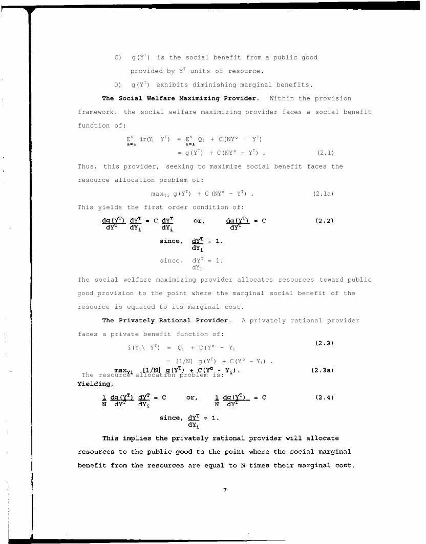
C) g(YT) is the social benefit from a public good

provided by YT units of resource.

D) g(YT) exhibits diminishing marginal benefits.

The Social Welfare Maximizing Provider. Within the provision

framework, the social welfare maximizing provider faces a social benefit

function of:

EN ir(Yi YT) = EN Qi + C(NY° - YT)

= g(YT) + C(NY° - YT) . (2.1)

Thus, this provider, seeking to maximize social benefit faces the

resource allocation problem of:

maxYi g(YT) + C (NY° - YT) . (2.1a)

This yields the first order condition of:

since, dYT = 1.dYi

The social welfare maximizing provider allocates resources toward public

good provision to the point where the marginal social benefit of the

resource is equated to its marginal cost.

The Privately Rational Provider. A privately rational provider

faces a private benefit function of:

i(Yi\ YT) = Qi + C(Y° - Yi

= [1/N] g(YT) + C(Y° - Yi) .

The resource allocation problem is:

Since g(YT) exhibits diminishing marginal benefits, the privately

rational provider will under-invest in the provision of the public good.

The two paradigms of choice lead to two competing models of

behavior type: for privately rational individuals the behavior described

by equation (2.4) and for social welfare maximizers the behavior

described by equation (2.2). Under specific parameter choices, these

theoretic descriptions of agent behavior can be tested against observed

experimental outcomes. The next section develops the basic experimental

decision environment faced by the subjects.

III. The Experimental Setting

The experiments used student volunteers recruited from the

undergraduate populations at Indiana University and the University of

Arizona. Before subjects were recruited from their respective classes,

the students were informed that, should they volunteer, they would be

making economic choices in a computerized decision environment. They

were also told that their earnings in this experimental environment

would be contingent upon their choices and the choices of their cohorts.

The subjects first participated in a trainer experiment to give them

experience in the decision environment. This trainer experiment used

the same decision environment as those used in this study, but had

different parameterizations.

The trained subjects were assigned a NovaNET computer terminal and

logged into the experiment. They then worked through a set of

computerized instructions explaining their particular decision

environment. A full transcript of the computerized instructions is in

Appendix A. In a subset of these experiments, the subjects made one-

period ahead forecasts of aggregate cohort investment choices. In these

experiments, the subjects read a supplementary instruction sheet

explaining the forecasting procedure after they finished the

computerized instructions. A full transcript of the supplementary

I

instructions is at the end of Appendix A. The experiment monitor

reviewed the additional instructions orally to make certain the subjects

understood the forecasting procedure. If the subjects had any questions

about the instructions, or had questions during the experiment, these

questions were directed to the experiment monitor. After the

instructions, the subjects were told they would be paid their

experimental earnings, in cash, in private, at the conclusion of the

experiment. They were instructed to refrain from all forms of inter-

subject communication and then they proceeded into the experiment.

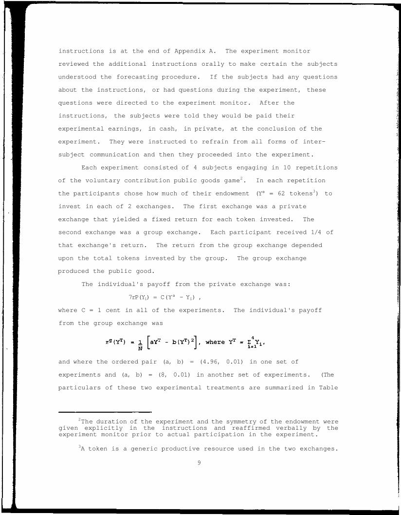
Each experiment consisted of 4 subjects engaging in 10 repetitions

of the voluntary contribution public goods game2. In each repetition

the participants chose how much of their endowment (Y° = 62 tokens3) to

invest in each of 2 exchanges. The first exchange was a private

exchange that yielded a fixed return for each token invested. The

second exchange was a group exchange. Each participant received 1/4 of

that exchange's return. The return from the group exchange depended

upon the total tokens invested by the group. The group exchange

produced the public good.

The individual's payoff from the private exchange was:

7rP(Yi) = C(Y° - Yi) ,

where C = 1 cent in all of the experiments. The individual's payoff

from the group exchange was

and where the ordered pair (a, b) = (4.96, 0.01) in one set of

experiments and (a, b) = (8, 0.01) in another set of experiments. (The

particulars of these two experimental treatments are summarized in Table

2The duration of the experiment and the symmetry of the endowment weregiven explicitly in the instructions and reaffirmed verbally by theexperiment monitor prior to actual participation in the experiment.

3A token is a generic productive resource used in the two exchanges.

9

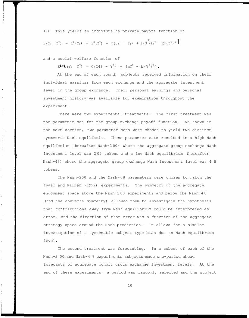
1.) This yields an individual's private payoff function of

i(Yi YT) = ip(Yi) + ig(YT) = C(62 - Yi) + 1/N (aY

T - b (YT)2)

and a social welfare function of

E4 i(Yi YT) = C(248 - YT) + [aYT - b(YT)2].

At the end of each round, subjects received information on their

individual earnings from each exchange and the aggregate investment

level in the group exchange. Their personal earnings and personal

investment history was available for examination throughout the

experiment.

There were two experimental treatments. The first treatment was

the parameter set for the group exchange payoff function. As shown in

the next section, two parameter sets were chosen to yield two distinct

symmetric Nash equilibria. These parameter sets resulted in a high Nash

equilibrium (hereafter Nash-2 00) where the aggregate group exchange Nash

investment level was 2 00 tokens and a low Nash equilibrium (hereafter

Nash-48) where the aggregate group exchange Nash investment level was 4 8

tokens.

The Nash-200 and the Nash-4 8 parameters were chosen to match the

Isaac and Walker (1992) experiments. The symmetry of the aggregate

endowment space above the Nash-2 00 experiments and below the Nash-4 8

(and the converse symmetry) allowed them to investigate the hypothesis

that contributions away from Nash equilibrium could be interpreted as

error, and the direction of that error was a function of the aggregate

strategy space around the Nash prediction. It allows for a similar

investigation of a systematic subject type bias due to Nash equilibrium

level.

The second treatment was forecasting. In a subset of each of the

Nash-2 00 and Nash-4 8 experiments subjects made one-period ahead

forecasts of aggregate cohort group exchange investment levels. At the

end of these experiments, a period was randomly selected and the subject

10

whose forecast was closest to his cohorts actual investment level was

paid an additional $3.00. This payoff scheme was selected because it

had no impact on the Nash nor the socially optimal incentive structure

and therefore no impact on the Nash nor the socially optimal strategies

Yet, it gave an incentive for the subjects to forecast accurately.

The preceding section outlined the general environment faced by

subjects. To make specific outcome predictions, the particular

parameterizations of each experiment are examined.

IV. Theoretic Solutions

The two paradigms of human interaction, coupled with the specific

functional forms in the experiments, yield two possible models of

subject behavior. These are the Nash model for the privately rational

and the social welfare maximizing model. This section develops

predictions made by these models.

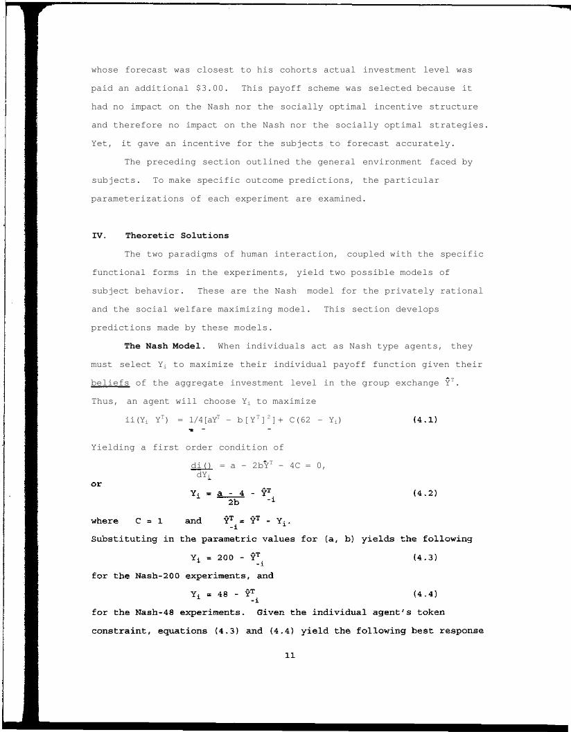
The Nash Model. When individuals act as Nash type agents, they

must select Yi to maximize their individual payoff function given their

beliefs of the aggregate investment level in the group exchange YT.

Thus, an agent will choose Yi to maximize

ii(Yi YT) = 1/4[aYT - b[YT]2]+ C(62 - Yi)

Yielding a first order condition of

di() = a - 2bYT - 4C = 0,dYi

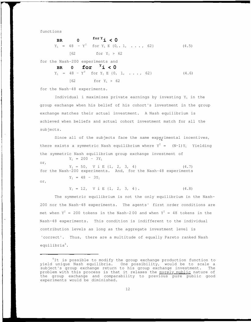
functions

BR 0 for Yi < 0

Yi = 48 - YT for Yi E {0,. 1, . . . , 62} (4.5)

[62 for Yi > 62

for the Nash-200 experiments and

BR 0 for Yi < 0Yi = 48 - YT for Yi E {0, 1, . . . , 62} (4.6)

[62 for Yi > 62

for the Nash-48 experiments.

Individual i maximizes private earnings by investing Yi in the

group exchange when his belief of his cohort's investment in the group

exchange matches their actual investment. A Nash equilibrium is

achieved when beliefs and actual cohort investment match for all the

subjects.

Since all of the subjects face the same experimental incentives,

there exists a symmetric Nash equilibrium where YT = (N-1)Yi Yielding

the symmetric Nash equilibrium group exchange investment ofYi = 200 - 3Yi

or,Yi = 50, V i E {l, 2, 3, 4} (4.7)

for the Nash-200 experiments. And, for the Nash-48 experiments

Yi = 48 - 3Yior,

Yi = 12, V i E {l, 2, 3, 4}. (4.8)

The symmetric equilibrium is not the only equilibrium in the Nash-

200 nor the Nash-48 experiments. The agents' first order conditions are

met when YT = 200 tokens in the Nash-2 00 and when YT = 48 tokens in the

Nash-48 experiments. This condition is indifferent to the individual

contribution levels as long as the aggregate investment level is

'correct'. Thus, there are a multitude of equally Pareto ranked Nash

equilibria4.

4It is possible to modify the group exchange production function toyield unique Nash equilibria. One possibility, would be to scale asubject's group exchange return to his group exchange investment. Theproblem with this process is that it relaxes the purely public nature ofthe group exchange and comparability to previous pure public goodexperiments would be diminished.

12

Social Welfare Optimization. A social welfare maximizing

individual will choose Yi to maximize the joint payoff function given

his beliefs of cohort investment levels. Or,

Substituting the parameters for the Nash-200 and Nash-48 experiments

into equation (4.10) yields

(4.11)

for the Nash-200 experiments and

Yi = 198 - YT, (4.12)

for the Nash-48 experiments.

Taking the subjects token endowments into consideration yields the

following best-response functions.

'0

for the Nash-48 experiments.

Using the symmetry of the incentive structure, a symmetric

solution emerges where

Yi = 3 50 - YT or

yielding

Y i = 6 2 V i G { l , 2, 3, 4}

for the Nash-200 experiments since subject's choices are constrained by

their endowmenr of 62 tokens each5. For the Nash-48 experiments,

5This is a unique solution, so the supergame solution is the repeatedplay of this solution. This is independent of symmetry since 62 tokens isa corner, given the subject's endowment.

13

Yi = 198 - YT. or Yi = 198 - 3Yi

yielding

Yi = 49.5 or the symmetric mixed strategy of Yi = {49, 50},

where 49 and 50 are each played with a probability of P = 0.5. The

symmetric mixed strategy solution is played since the subjects must make

integer valued investments. Again, there are a multitude of equally

Pareto ranked solutions. Only the symmetric solution will be

considered.

Three Mixed Subject Type Solutions. There are also three

solutions considered that involve mixed subject types. The first is

when one subject is maximizing social welfare while the other three

subjects are privately rational. The second is when two subjects are

social welfare maximizers and two subjects are privately rational. The

third is when three subjects are social welfare maximizers and the

remaining subject is privately rational. These solutions are calculated

assuming each subject knows his type and the types of his cohorts.

In the Nash-200 experiments, the social welfare maximizing subject

has insentive to contribute 62 tokens to the group exchange regardless

of the contribution levels of his cohorts. So, let (n) be the number of

privately rational subjects in the experiment, leaving (4 - n) social

welfare maximizers. Let Y and Ys be the symmetric privately rational

and social welfare maximizing investment levels respectively. The (n)

privately rational subjects must satisfy:

nYp = 200 - (4 - n)Ys or Yp = 200/n - (4 - n)/n 62.

Yielding, YP = 46, Ys = 62 for n = 3YP = 38, Ys = 62 for n = 2YP = 14, YS = 62 for n = 1

In the Nash-48 experiments, the privately rational subject will

invest in the group exchange to satisfy:

nYp = 48 - (4 - n)Ys. (4.15)

In addition, the social welfare maximizing subject will invest in the

group exchange to satisfy:

14

(4 - n)Ys = 198 - nYp. (4.16)

Case 1: n = 1

From the endowment constraint, Yp < 62. Substituting this into

equation (4.16) yields 3YS > 136. Thus, equation (4.15) becomes Yp <

-8 8 or Yp = 0; yielding Ys = 62.

Case 2: n = {2, 3}

From the endowment constraint, Ys is non-negative, so from

equation (4.15) nYp < 48. Substituting nYp < 48 into equation (4.16)

yields (4 - n)Ys > 150. Imposing the token constraint yields, Ys = 62

and Yp = 0 for n = {2, 3} .

Summarizing, social welfare maximizing and privately rational

agents will invest along their respective best-response functions. If

they all forecast cohort group exchange investment levels accurately,

then they will achieve one of the two symmetric solutions or one of the

three mixed solutions. These solutions are characterized by strategy

and summarized in Table 2.

V. The Analysis Of Results

In addition to following a best-response path, subjects having

solved one of the five solutions might unilaterally play that solution

and wait for cohorts to converge to the anticipated solution. Thus, the

experimental environment yields two broad behavioral categories for

investment in the group exchange investment.

1) Individual providers invest into the group exchangeas predicted by one of their best-responsefunctions.

2) Individual providers myopically invest tokens intothe group exchange as predicted by one the fivesolution types.

The predicted outcomes associated with these two categories and the

underlying maximization problems can be compared to the outcomes

achieved by subjects participating in the experimental decision

environment.

15

(4 - n)Ys = 198 - nYp. (4.16)

Case 1: n = 1

From the endowment constraint, Yp < 62. Substituting this into

equation (4.16) yields 3YS > 136. Thus, equation (4.15) becomes Yp <

-88 or Yp = 0; yielding Ys = 62.

Case 2: n = {2, 3}

From the endowment constraint, Ys is non-negative, so from

equation (4.15) nYp < 48. Substituting nYp < 48 into equation (4.16)

yields (4 - n)Ys > 150. Imposing the token constraint yields, Ys = 62

and Yp = 0 for n = {2, 3} .

Summarizing, social welfare maximizing and privately rational

agents will invest along their respective best-response functions. If

they all forecast cohort group exchange investment levels accurately,

then they will achieve one of the two symmetric solutions or one of the

three mixed solutions. These solutions are characterized by strategy

and summarized in Table 2.

V. The Analysis Of Results

In addition to following a best-response path, subjects having

solved one of the five solutions might unilaterally play that solution

and wait for cohorts to converge to the anticipated solution. Thus, the

experimental environment yields two broad behavioral categories for

investment in the group exchange investment.

1) Individual providers invest into the group exchangeas predicted by one of their best-responsefunctions.

2) Individual providers myopically invest tokens intothe group exchange as predicted by one the fivesolution types.

The predicted outcomes associated with these two categories and the

underlying maximization problems can be compared to the outcomes

achieved by subjects participating in the experimental decision

environment.

15

A summary of these comparisons show that of the 76 subjects

participating in the 19 experiments, 49 (64%) followed group exchange

investment strategies consistent with one of the two investment

categories. Another 12 (16%) subjects followed an investment strategy

of equally dividing tokens between the two exchanges and the final 15

(20%) subjects' investments into the group exchange were inconsistent

with all of the above.

These summary results were compiled from subject type sorting

procedures derived from the two categories of subject investment. The

first classification scheme sorted for subjects following one of their

best-response paths. The second classification scheme sorted for

subjects myopically following one of the five solution types. For

reporting purposes, a subject whose investment path followed a best-

response path and also followed a myopic solution path was classified

according to the best response scheme.

Best Response Classifications. Social welfare maximizing subjects

must invest in the group exchange as predicted by equations 4.5 or 4.6

and Nash type subjects must invest as predicted by equations 4.14 or

4.15. These best-response functions are dependent on cohort group

exchange investment levels. Thus, in order to choose a best response

the subjects must first forecast their cohort's group exchange

investments. In a subset of the experiments, these forecasts were

expressly solicited from the subjects. In the remaining experiments, a

forecast mechanism must be assumed. For the purpose of this analysis,

the subjects were assumed to forecast cohort group exchange investment

levels perfectly.

Perfect Foresight. Given this forecast mechanism, the subjects'

best-response functions generate a pair of predicted group exchange

investment paths. One best-response path associated with social welfare

maximizing and one associated with Nash behavior. Each subject's actual

investment path was paired, period by period, with the two perfect

16

foresight best-response paths. The Wilcoxon matched pairs test was used

to determine whether a subject's investment path was significantly-

different from the predicted best-response paths, at a significance

level of a = 0.05. In cases where the best-response path was at a

corner solution for all 10 investment rounds the one-tailed matched

pairs t-test was used6 for classifying subject type7.

Using this procedure, the subjects were sorted into one of three

types.

1) Nash type providers, for those subjects whoseinvestment path was not significantly different fromthe Nash best-response path.

2) Social type providers, for those subjects whoseinvestment paths were not significantly differentfrom the social welfare maximizing best-responsepath.

3) None, for those subjects whose investment paths weresignificantly different from both best-responsepaths.

Table 3 reports the results of this classification process. As

seen in the third column, of the 76 subjects participating in the

provision experiments, 23 (30%) invested tokens into the group exchange

in a way consistent with the Nash best-response path and 11 (14%)

invested in a way consistent with the social welfare maximizing best-

response path.

These results come from pooling ten Nash-200 and nine Nash-48

experiments. As Isaac and Walker (1992) found asymmetric investment

results between these two experimental treatments, it is useful to look

6The Wilcoxon test was inappropriate since all ranks would beconstrained either positive or negative. Therefore, the minimum of thesum of the positive or negative ranks would be zero. The test wouldalways reject the hypothesis that the actual investment path and the bestresponse path have the same distribution. The t-test will suffer due tothe truncation in the data and will tend to over reject but is more robustin this environment.

7In addition, for one subject in the Nash-48 experiments, due tocohort investment patterns, the Nash and social welfare best responsepaths were identical. This subject was arbitrarily classified as a Nashtype provider.

17

closer for corresponding asymmetries in subject type results.

The 40 subjects in the Nash-200 experiments, reported in the first

column of Table 3, invested so that 11 (28%) of the subjects fit the

classification of Nash type providers and 9 (22%) as social welfare

maximizing actors. Figure la records the average per-period deviations

from the best-response path (BRP) for those classified as Nash actors or

social actors. As seen, the social welfare maximizing actors closely

track their BRP. The Nash actors' path is more erratic, but the BRP

reference line is a good estimate of central tendency.

Of the 36 subjects in the Nash-48 experiments, reported in column

2 of Table 3, 12 (33%) of the subjects fit the classification of Nash

type actors, 2 (6%) fit the classification of social welfare maximizing

actors. Figure lb shows the average deviation from the BRP for the

Nash-48 experiments. Though the average deviations track the BRP less

closely in Figure lb than in Figure la, they still show a tendency

toward the BRP. Thus, adding modest support to the classification

results.

The particular classification scheme, described above, suggests

there are fewer social welfare maximizing actors in the Nash-48

experiments than in the Nash-200. A more detailed investigation of this

and other differences will be presented when the experimental treatment

effects are examined.

Forecasting Experiments. In the experiments where forecasts were

solicited, it was possible to construct the subject's best-response path

given his reported forecasts. Thus, the determination of a subject's

underlying paradigm of rationality was not contingent upon an assumed

forecasting mechanism.

There were 6 forecasting experiments. As reported in last column

of Table 4, of the 24 subjects who participated in these experiments, 5

(21%) followed a strategy not significantly different from their Nash

best-response paths. The first column of Table 4 reports 3 (25%) of the

18

12 subjects who participated in the Nash-200 experiments followed Nash

type strategies. The second column of Table 4 reports 2 (17%) of the 12

subjects who participated in the Nash-48 experiments followed Nash type

strategies. None of the subjects were classified as following social

welfare maximizing strategies.

Myopic Solution Classifications. It is interesting to note that 7

(58%) of the subjects in the Nash-48 forecasting experiments invested

around 31 tokens into the group exchange. In all, 4 0 (57%) of their

group exchange investments fell in the 3 token range from 30 to 32.

This demonstrates the existence of a group of subjects whose investment

strategy focuses on the midpoint of their endowment space. There are

other potential focal points for investors. The second investment

category addresses the issue of subjects myopically investing into the

group exchange consistent with one of the five solution types reported

in Table 2. A subject's actual group exchange investment path was

compared to the predicted solutions. If the subject's investment path

was sufficiently close, as determined by a paired t-test at a

significance level of a = 0.05, to a theoretic outcome, that subject was

classified as following the associated maximization problem8. For

corner solution outcomes, the associated t-test was one tailed. For the

others, the associated t-test was two tailed.

Using this sorting criteria, as seen in the third column of Table

5, 16 (21%) subjects' behavior was consistent with a social welfare

maximizing path and 25 (33%) with a Nash path. Of the 35 (46%) subjects

whose investment patterns were inconsistent with the solution paths, 14

(18%)9 of them invested into the group exchange consistent with 31

8The t-test was used for consistency since the Wilcoxon test would beinappropriate due to corner solution problems for 10 of the 16 solutiontypes.

9The difference between the number equal-dividers reported here andthe number of equal-dividers reported in the summary is due to the factthat 2 of these agents have best response paths consistent with a mid-division strategy.

19

tokens; or equally dividing their token endowment between the two

exchanges.

Nash-200 Experiments. Of the 40 subjects participating in the

Nash-200 experiments, as seen in the first column of table 5, 19 (48%)

were consistent with one of the Nash strategies and 12 (30%) with the

social welfare maximizing strategy. Only 9 (22%) subjects failed to

invest into the group exchange as predicted by one the solutions.

In all, 11 of 12 subjects classified as social welfare maximizers

invested in the group exchange in a way not significantly different from

the unique social optimum of 62 tokens. The top trace in Figure 2a

shows how closely the "average per-period investments" of these 11

subjects came to the symmetric social optimum (SSO). Of the 110

investment decisions made by these 11 subjects, 92 (84%) were at 62

tokens and only 11 (10%) investment decisions were below 60 tokens

yielding a distribution of group exchange investments tightly packed

around 62 tokens.

A twelfth subject invested 62 tokens in the group exchange for

each of his last five investment decisions. Although his investment

path was significantly different from the socially welfare maximizing

path, he was counted as being socially rational.

Of the 19 subjects classified as Nash agents, 12 invested in the

group exchange not significantly different from the symmetric Nash

equilibrium of 50 tokens. In addition, 5 followed an investment path

consistent with the mixed subject solution with two social welfare

maximizers and two Nash actors. The last 2 followed an investment path

consistent with the mixed subject solution with one social welfare

maximizer and three Nash actors. The middle trace in Figure 2a tracks

the average per-period investment decisions of the 12 symmetric Nash

subjects and shows how close they come to the symmetric Nash equilibrium

(SNE) investment level. Of the 12 0 group exchange investments made by

these subjects, 19% were at 50 tokens, and 45% fell within the 11 token

20

investment level range of 45 to 55 tokens.

Nash-48 Experiments. Of the 36 subjects who participated in the

Nash-48 experiments, shown in the middle column of Table 5, 6 (17%)

behaved consistently with a Nash solution and 4 (11%) with a social

welfare maximizing solution.

Three of the Nash type actors and 3 of the social welfare

maximizers followed paths not significantly different from their

respective symmetric solutions. In both cases the number of investments

made at the symmetric solution levels, 50 tokens for social welfare

maximizing and 12 tokens for Nash, were not significantly higher than

expected by random investment at a = 0.05. This result raises questions

as to whether the subjects were focusing their investment at these two

solutions. Figure 2b shows how erratic the average investment paths

are, and shows distinct downward trends. This is not consistent with

the predictions of the symmetric solutions. The final 3 Nash type

actors invested in a way not significantly above zero tokens, the mixed

subject type Nash solution where at least one of the subjects is a

social welfare maximizer. Of the 3 0 investment decisions made by these

subjects, 25 were at zero tokens. This is strong evidence that these

subjects were focusing their investments at zero tokens.

The average investment of 14 of the 2 6 remaining subjects was not

significantly different from 31 tokens, with 64 (46%) of their 140

investment decisions in the 7 token mid-range from 28 to 34 tokens.

Even though these subjects tended to invest 31 tokens into the group

exchange, their per-period average investment had a definite downward

trend toward the Nash equilibrium investment level of 12 tokens. In

fact, their average per-period investment fell 8.5 tokens from 3 3.29

tokens to 24.79 tokens over the last five periods10.

10In fact, the least squares linear approximation of these subjects'average investment path,

Avg. Inv. = Intercept + j3 (Period) + v,where v ~ n(0, a),

yields B = -0.94, significantly less than zero at a = 0.05 with a test

21

End Period Effects. Since the subjects in all of the experiments

were explicitly informed that the experiments were ten periods, game

theory suggests they should treat the last period as a one-shot

voluntary contribution public goods game. Thus, subjects should invest

into the group exchange as predicted by the solutions in Table 2. Over

all, 16 (21%) of the end period investments matched a Nash investment

and 15 (20%) matched a social welfare maximizing investment. Random

investment suggests that 7 (9%) of investments should fall on one of the

Nash solutions and 4 (5%) of investments should fall on one of the

social welfare maximizing solutions. The Z-test for sample proportions

show both Nash end-period investment and social welfare maximizing end-

period investment significantly higher than predicted by random

investment with Z-values of Z = 3.61 and Z = 6.00 respectively.

Treatment Effects on Subject Type. As forecasting is a new

treatment in public good experiments, it is important to know whether it

impacts subject behavior. An argument can be made that explicit

forecasting induces subjects to focus on one of their two best-response

functions. This added focus would result in higher proportions of

subjects following one of their perfect foresight best-response paths.

To test this hypothesis, a contingency table separating subjects by

experimental design characteristics and behavior type was used. A 2-

tailed Z-test of significance of difference between independent sample

proportions was used to measure the impact of the design characteristic

on subject behavior. The first test compares subject behavior in

forecasting experiments to behavior in non-forecasting experiments,

holding design characteristics constant through the contingency table.

Table 6 reports the Z-test statistics for the comparisons with the

corresponding p-value in parentheses below. The first cell in Table 6

reports significantly (at a = 0.05) fewer social welfare maximizing

statistic of t = -7.67 and an intercept at 36.03. The negativecoefficient B confirms the downward trend in the investment patterns ofthese subjects.

22

subjects in the forecasting experiments than in the non-forecasting

experiments, holding the Nash-200 design constant. There are, also,

fewer Nash actors and a significant increase in subjects following

neither paradigm of rationality in the Nash-200 forecasting experiments

than in the Nash-200 non-forecasting experiments. In the Nash-48

experiments (reported in the second column of Table 6) the forecasting

treatment shows no significant effect on subject behavior. Thus, the

proposition that forecasting would increase observed best response

behavior can be rejected. If anything, forecasting in these experiments

has a tendency to decreased proportions of subjects following a best-

response path; contradicting the focusing effect that was expected.

The other experimental treatment in this study was the group

exchange production function. Analyzing aggregate behavior, Isaac and

Walker (1992) found an upward investment bias in Nash-48 experiments

relative to a corresponding downward bias in the Nash-200 experiments.

This implied that Nash equilibrium levels introduced a systematic effect

which could not be entirely explained by random error. Given a

systematic bias on group level investment associated with Nash

equilibrium level, looking for effects associated with the Nash

equilibrium at the individual level is a natural extension. Table 7

reports the Z-test values derived from testing the significance of

difference in sample proportions of subject type classifications between

the Nash-200 and Nash-48 experiments. The group exchange production

function treatment shows no significant (at a = 0.05) nor consistent

effect on subject behavior.

VI. Concluding Comments

This research investigated individual provision decisions in an

experimental voluntary contribution public good environment. Subjects

were classified according to the type of provision behavior they

exhibited. Over all, 64% of the subjects participating in the public

23

good experiments were classified as following one of the paradigms of

rationality. The behavior of 43% of the subjects was consistent with

Nash strategies and the behavior of 21% of the subjects was consistent

with social welfare maximizing strategies. With one of five subjects

following socially rational strategies, it is easy to see why, in

aggregate, investment levels are significantly above those predicted by

the Nash equilibrium.

Another 16% of the subjects (all from Nash-48) followed the

strategy of equally dividing their token endowment between the group and

private exchanges. As discussed in Section V, these subjects'

investments trended downwards toward the Nash equilibrium level. This

leaves 20% of the investment patterns unclassified.

The experiments had two treatment variables. The first was

forecasting and the second was the Nash equilibrium level. The theory

of objective maximizing agents is mute to these two treatments, implying

they should have no effect on subject behavior. The effects of

forecasting on the classification results was consistent across

experiment type. Its observed impact on subject type classifications

implies explicit forecasting hampers subjects from finding their perfect

foresight best-response paths. The impact of Nash equilibrium level on

subject behavior was not significant.

Over all, this investigation of individual level behavior extends

our understanding of aggregate level results presented in past studies

of the voluntary contribution mechanism for public goods. In

particular, it shows that a large proportion of the subjects have public

good contribution patterns consistent with theoretic predictions. It

also shows that Nash type behavior is not the dominant behavior in this

environment, with a full 57% of the subjects exhibiting non-Nash

behavior. Although neither aggregate Nash nor aggregate socially

optimal behavior is observed, the observed behavior of most subjects is

consistent with one of the two underlying paradigms of rationality.

24

APPENDIX A Transcript of Instructions

This experiment is a study of group and individualexchange behavior. The instructions are simple, andif you follow them carefully and make goodinvestment decisions, you may earn a CONSIDERABLEAMOUNT OF MONEY which will be paid to you in cash atthe end of the experiment. Various researchfoundations have provided funds for this research.

You are one person in a group of 4.Each of you will be given an investmentaccount with a specific number of tokens init. All tokens must be invested to turn theminto income.

There are two ways you can earn money byinvesting your tokens. Press -NEXT- tofind out more about them.

1. The INDIVIDUALEXCHANGE

For each token youinvest in the individualexchange you get:1 Cents per token.

For example:

If you invest 55tokens in the individualexchange, you earn:$ 0.55.

If you invest 140tokens in the individualexchange, you earn:$ 1.40.

2. The GROUP EXCHANGE

The return on your invest-ment in the group exchangeis not so easilydetermined.Your earnings depend uponthe total investment inthe group exchange (yourinvested tokens plus allof the other tokensinvested by the otherpeople in your group).

Press NEXT to find outmore about the groupexchange; press BACK toreview the previousinstructions.

You and 3 other people are members of a group.

When you invest in the group exchange, how muchmoney you get back depends on what you do and also onhow much the other group members invest.

The more the GROUP invests, the more you all getfrom the GROUP exchange.

In your group, each person has an investment accountwith a specific number of tokens in it.

The group as a whole has 248 tokens.YOU have 62 tokens .

When you invest in the group exchange, the tokensyou invest are no longer yours. THEY BECOME THEPROPERTY OF THE GROUP!

The money that the invested tokens earn is alsothe property of the group. This money is divided

25

up at the end of the period. Each person gets anequal share out of every group dollar.

IT DOES NOT MATTER WHO INVESTS THE TOKEN IN THEGROUP EXCHANGE. Every dollar is divided up thisway.

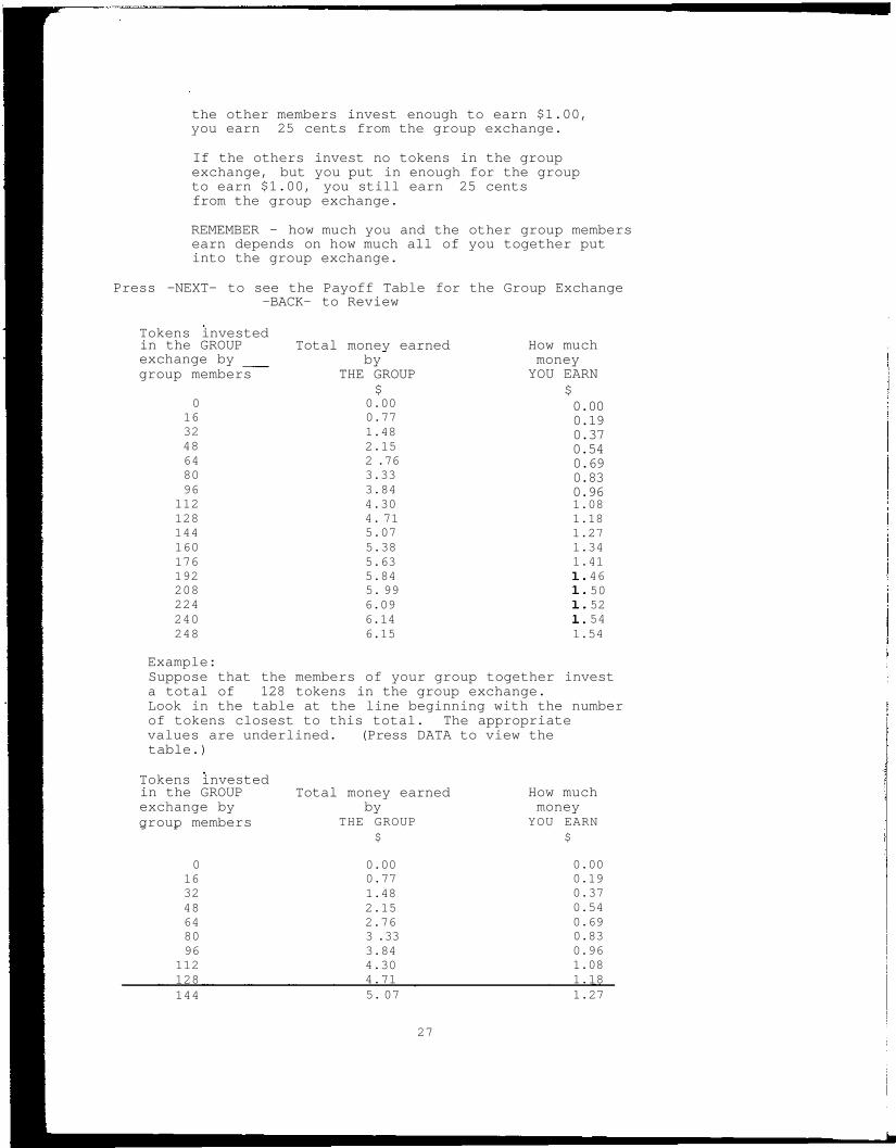
For example:If you put no tokens in the group exchange, butthe other members invest enough to earn $1.00,you earn 25 cents from the group exchange.

If the others invest no tokens in the groupexchange, but you put in enough for the groupto earn $1.00, you still earn 25 centsfrom the group exchange.

REMEMBER - how much you and the other group membersearn depends on how much all of you together putinto the group exchange.

Press -NEXT- to see the Payoff Table for the Group Exchange-BACK- to Review

Tokens investedin the GROUPexchange bygroup members

016

Total money earnedby

THE GROUP$

0.000.77

How muchmoneyYOU EARN

$0.00

You and 3 other people are members of a group.

When you invest in the group exchange, how muchmoney you get back depends on what you do and also onhow much the other group members invest.

The more the GROUP invests, the more you all getfrom the GROUP exchange.

In your group, each person has an investment accountwith a specific number of tokens in it.

The group as a whole has 248 tokens.YOU have 62 tokens .

When you invest in the group exchange, the tokensyou invest are no longer yours. THEY BECOME THEPROPERTY OF THE GROUP!

The money that the invested tokens earn is alsothe property of the group. This money is dividedup at the end of the period. Each person gets anequal share out of every group dollar.

IT DOES NOT MATTER WHO INVESTS THE TOKEN IN THEGROUP EXCHANGE. Every dollar is divided up thisway.

For example:If you put no tokens in the group exchange, but

26

the other members invest enough to earn $1.00,you earn 25 cents from the group exchange.

If the others invest no tokens in the groupexchange, but you put in enough for the groupto earn $1.00, you still earn 25 centsfrom the group exchange.

REMEMBER - how much you and the other group membersearn depends on how much all of you together putinto the group exchange.

Press -NEXT- to see the Payoff Table for the Group Exchange-BACK- to Review

How muchmoneyYOU EARN

$0.000.190.370.540.690.830.96

Tokens investedin the GROUPexchange bygroup members

0163248648096

112128144160176192208224240248

Total money earnedby

THE GROUP$

0.000.771.482.152 .763.333.844.304. 715.075.385.635.845. 996.096.146.15

1.081.181.271.341.41

46505254

1.54

Example:Suppose that the members of your group together investa total of 128 tokens in the group exchange.Look in the table at the line beginning with the numberof tokens closest to this total. The appropriatevalues are underlined. (Press DATA to view thetable.)

Tokens investedin the GROUPexchange bygroup members

0163248648096

112128

Total money earnedby

THE GROUP$

0.000.771.482.152.763 .333.844.304.71

How muchmoney

YOU EARN$

0.000.190.370.540.690.830.961.081.18

144 5. 07 1.27

27

160176192208224240248

5.38 1.345.63 1.415.84 1.465.99 1.506.09 1.526.14 1.546.15 1.54

Look to the underlined values.

You saw from the table that the group gets $ 4.71.from the exchange. Every group member gets $ 1.18.from the exchange.You would receive $ 1.18 from the group exchange.WHETHER OR NOT YOU DEPOSIT ANY OF YOUR TOKENS IN THEEXCHANGE!

When you invest, you can divide your tokens in any wayyou want. That is, you can:

a. put all of them into the group exchangeb. put all of them into the individual exchangec. put some of them into the group exchange and

some of them into the individual exchange.

You will have 10 Trials in which you make investmentdecisions. The profits you make are stored after eachTrial and the total profits from all Trials paid to youat the end of the Experiment.

When you are asked how you want to invest,you may put all, some, or none of your 62 tokensin the group exchange, and put the remaining tokens inthe individual exchange. After you and everyone else inyour group has had a chance to invest at this first stage,you will be shown how many of the group's 248 tokenshave been put in the group exchange, and how many havebeen put into the individual exchange. You will also betold your earnings from the group exchange, from theindividual exchange, and your total earnings.

To give you practice in entering your investments,let's go through an example. Your screen willshow the same information it will contai7 in theactual experiment. Only the directions in thebox will not be available during the experiment.

You will be able to view your earnings fromeach of the previous TRIALS at the beginningof a new investment TRIAL. Press -DATA- toview the tables now.

TOTAL TRIALI 1 2 3 4 5 6 7 8 9NV g r pE 124 117 123 120 100 116 138 123 131ST ind 124 131 125 128 148 132 110 125 117ED

28

The token investment behavior of the group will betotaled and shown in the table above.

TRIAL1 2 3 4 5 6 7 8 9

YOURPR g r p 1 . 1 1 . 1 1 . 1 1 . 1 0 . 9 1 . 1 1 . 2 1 . 1 1 . 2 0OF i n d 0 . 6 0 . 6 0 . 6 0 . 6 0 . 6 0 . 6 0 . 6 0 . 6 0 . 6 2IT o t a l 1 . 7 1 . 7 1 . 7 1 . 7 1 . 6 1 . 7 1 . 8 1 . 7 1 . 8 2

The profit level from each TRIAL will be enteredin the TABLE above.

Press BACK to return to the investment page.Profits at the end of Trial (9)= $17.70

You have 62 tokens.

Suppose you decide to put 32 tokens in the groupexchange.

How many tokens do you wish to invest in the groupexchange? > 32Press EDIT to correct or change your bid; pressNEXT to enter your bid.

Type 32 after the arrow, then press NEXT toenter your answer.

Now you have 3 0 tokens left to invest in theindividual exchange. Press NEXT to continue display.

How many tokens do you wish to invest in theindividual exchange? > 30

Your group and individual investments together musttotal 62 . You must invest all of your tokens.Press EDIT to correct or change your bid; pressNEXT to enter your bid.

Type 3 0 after the arrow, then press NEXT toenter your answer.

If you wish to change your investment decision atthis time, press shift-BACK and redo the investmentprocess. If you are satisfied with your decisions,

At this point, you can press shift-BACK to change yourinvestment decisions for this period. You may do sonow if you wish to review the practice trial up tothese instructions. If you understand the proceduresso far, press NEXT.

RESULTS

You earned $ 1.18 from the group exchange.You earned $ 0.3 0 from the individual exchange.Total earnings = $ 1.4 8

29

Total token investment in group exchange = 12 8Total token investment in individual exchange = 120

IMPORTANT NOTICE

REMEMBER: At the end of the experimentyou receive the sum of your profits fromall TRIALS.

DO NOT SPEAK TO ANY OTHER PARTICIPANT!

The individual exchange gives you a sure return.Also, you have a chance to earn money from thegroup exchange if any members invest in it.

The group exchange gives you a chance to make morefrom your tokens invested. But, the earnings from theGroup Exchange will depend on the investment decisionof all participants.

NOTE: Your individual decision on how much youinvest in the private exchange and in thegroup exchange is not known by the otherparticipants. Only information on totalgroup investment is given to each person.

Do not press NEXT until you are ready to enterthe experiment. Once you press NEXT you willnot be able to review the instructions. PressBACK to review the instructions in reverse order;press shift-BACK to review the instructions intheir entirety; press NEXT only if you understandall of the instructions.

You will not be able to return to the instructionsafter leaving this page. If there is any doubtin your mind press BACK.

Once you press NEXT there is no turning back.Press NEXT only if you fully understand theinstructions.

30

ADDITIONAL INSTRUCTIONS

Please read these carefully

At the end of each investment period the computer will display a screenwhich shows the results of the recently completed period. After viewingthe results you can move into the next decision period. Once you haveentered the next decision period, you have many options. These includereviewing the history of decisions, entering a screen which allows youto calculate potential scenarios, and investing in the current period.

Before making your investment decision, you are to make a prediction onwhat you think the total investment of the others will be in the groupaccount. Your prediction of the others investment will be the totalinvestment you anticipate in the group account minus what you plan toinvest in the group account. You will then write this number downbeside the appropriate period on the sheet provided for you.

An example: If you intend to invest 20 tokens in the group account inperiod 1 and you expect the total investment in the group account to be80 tokens in period 1, then the amount you expect the others to investin period 1 will be 80 - 20 = 60. You would then write 60 in the spacebeside period 1 on the worksheet provided.

REMEMBER: It is important that you record only the investment in thegroup account you expect the others to make.

At the end of the experiment an investment period will be randomlyselected and the individual whose prediction of the total market-2investment of others is closest to the actual for that period willreceive an additional $3.00. This payment will be divided for ties.

31

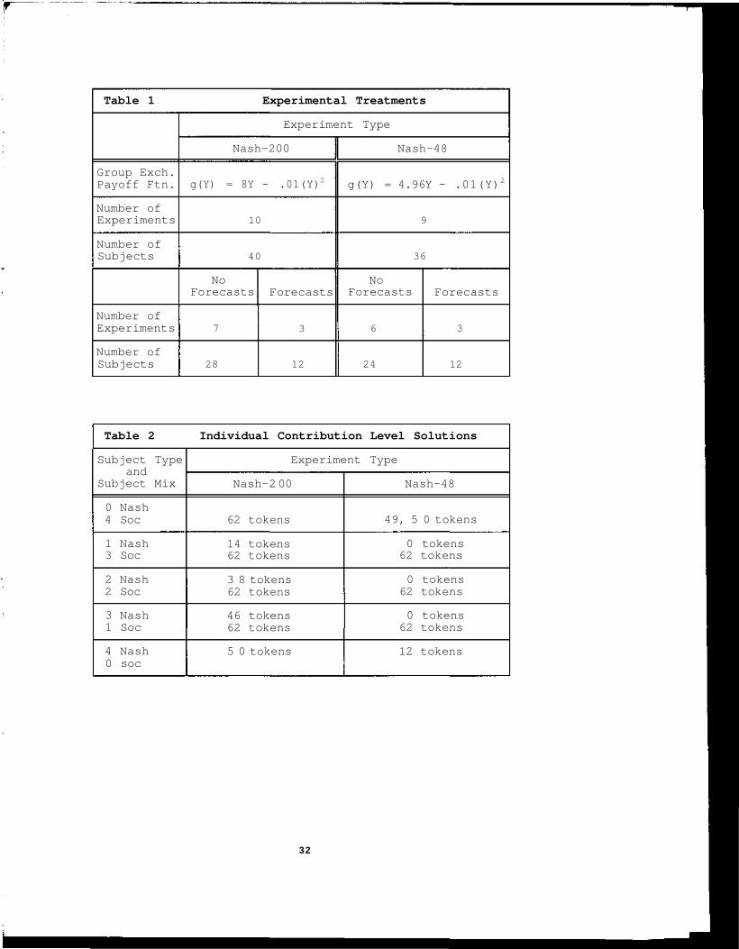
Table 1 Experimental Treatments

Group Exch.Payoff Ftn.

Number ofExperiments

Number ofSubjects

Number ofExperiments

Number ofSubjects

Experiment Type

Nash-200

g(Y) = 8Y - .01(Y)2

10

40

NoForecasts

7

28

Forecasts

3

12

Nash-48

g(Y) = 4.96Y - .01(Y)2

9

36

NoForecasts

6

24

Forecasts

3

12

Table 2 Individual Contribution Level Solutions

Subject Typeand

Subject Mix

0 Nash4 Soc

1 Nash3 Soc

2 Nash2 Soc

3 Nash1 Soc

4 Nash0 soc

Experiment Type

Nash-2 00

62 tokens

14 tokens62 tokens

3 8 tokens62 tokens

46 tokens62 tokens

5 0 tokens

Nash-48

49, 5 0 tokens

0 tokens62 tokens

0 tokens62 tokens

0 tokens62 tokens

12 tokens

32

Table 3 Number of Individuals Investing in a Way NotSignificantly Different From One of their BestResponse Functions Under the Perfect ForesightAssumption.

SocialWel. Max.

PrivatelyRational

Neither

Experiment Type

Nash-200

9(22%)

11(28%)

20(50%)

Nash-48

2(6%)

12(33%)

22(61%)

Total

11(14%)

23(30%)

42(55%)

Table 4 Number of Individuals Investing in a Way NotSignificantly Different From One of their BestResponse Functions Given Actual Forecast Data.

SocialWel. Max.

PrivatelyRational

Neither

Experiment Type

Nash-200

0(0%)

3(25%)

9(75%)

Nash-48

0(0%)

2(17%)

10(83%)

Total

0(0%)

5(21%)

19(79%)

For one of the subjects assigned as privately rational in the Nash-200experiments, the social and Nash best-response paths were identical.This subject was arbitrarily assigned as privately rational.

33

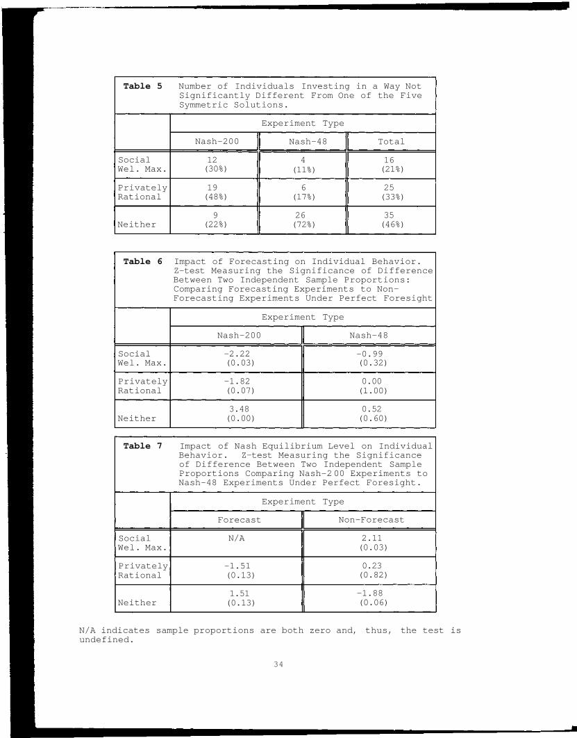
Table 5 Number of Individuals Investing in a Way NotSignificantly Different From One of the FiveSymmetric Solutions.

SocialWel. Max.

PrivatelyRational

Neither

Experiment Type

Nash-200

12(30%)

19(48%)

9(22%)

Nash-48

4(11%)

6(17%)

26(72%)

Total

16(21%)

25(33%)

35(46%)

Table 6 Impact of Forecasting on Individual Behavior.Z-test Measuring the Significance of DifferenceBetween Two Independent Sample Proportions:Comparing Forecasting Experiments to Non-Forecasting Experiments Under Perfect Foresight

SocialWel. Max.

PrivatelyRational

Neither

Experiment Type

Nash-200

-2.22(0.03)

-1.82(0.07)

3.48(0.00)

Nash-48

-0.99(0.32)

0.00(1.00)

0.52(0.60)

Table 7 Impact of Nash Equilibrium Level on IndividualBehavior. Z-test Measuring the Significanceof Difference Between Two Independent SampleProportions Comparing Nash-2 00 Experiments toNash-48 Experiments Under Perfect Foresight.

SocialWel. Max.

PrivatelyRational

Neither

Experiment Type

Forecast

N/A

-1.51(0.13)

1.51(0.13)

Non-Forecast

2.11(0.03)

0.23(0.82)

-1.88(0.06)

N/A indicates sample proportions are both zero and, thus, the test isundefined.

34

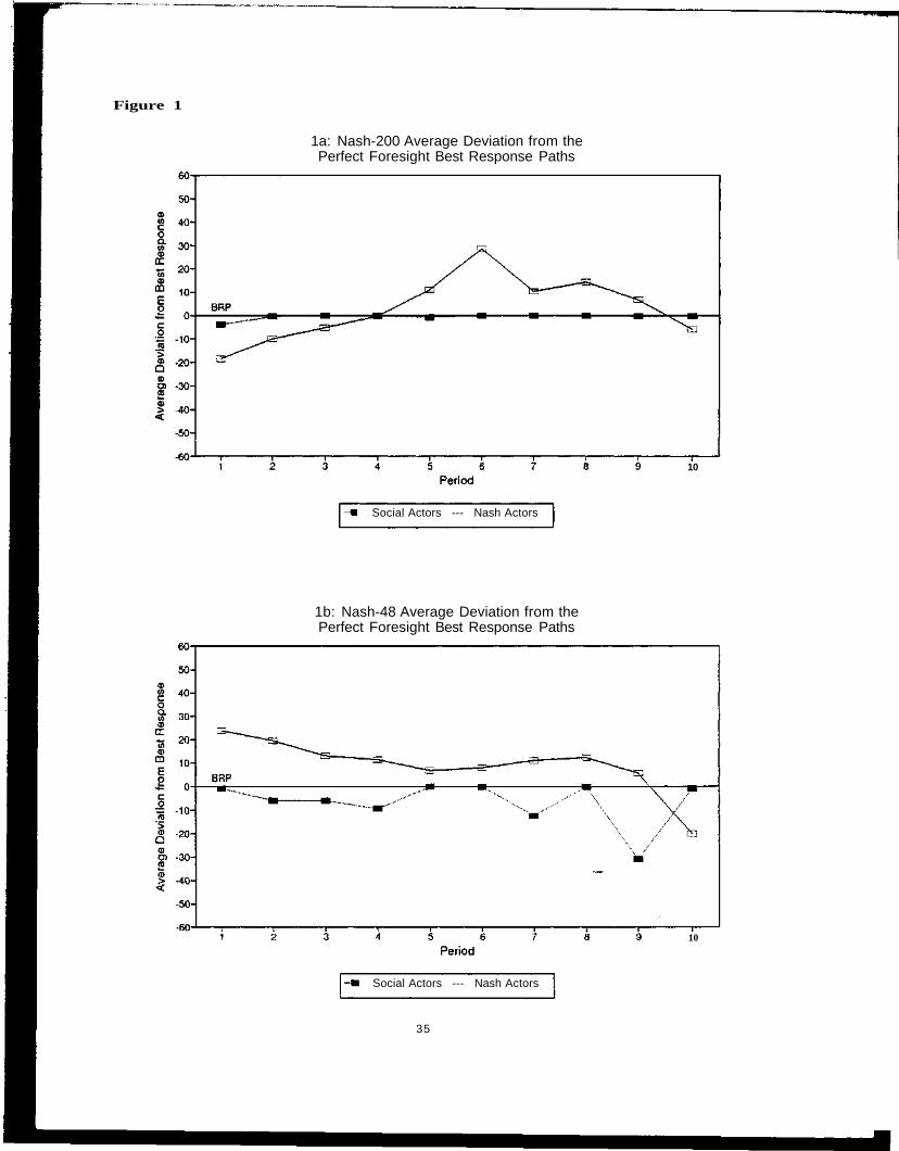
Figure 1

1a: Nash-200 Average Deviation from thePerfect Foresight Best Response Paths

10

Social Actors --- Nash Actors

1b: Nash-48 Average Deviation from thePerfect Foresight Best Response Paths

10

Social Actors --- Nash Actors

35

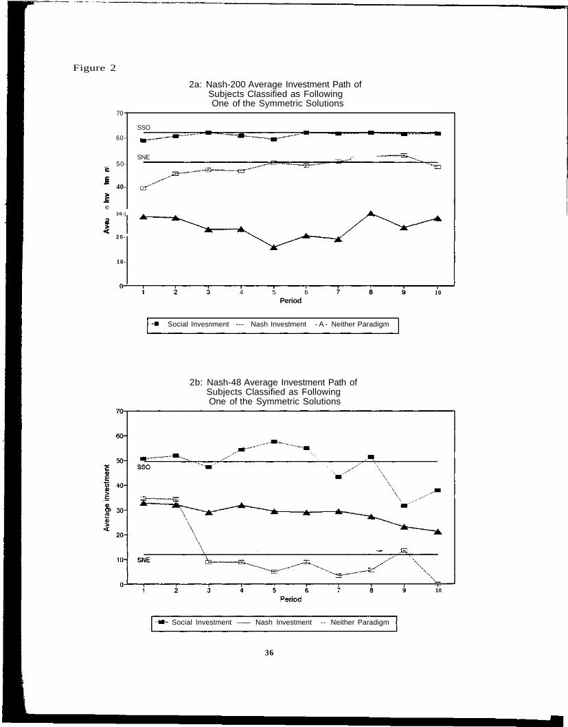
Figure 2

70

2a: Nash-200 Average Investment Path ofSubjects Classified as FollowingOne of the Symmetric Solutions

60-

_ 50-

40-

©30 - |

2

2 0 -

10-

SSO

SNE --

4 5 6Period

10

Social Invesnment --- Nash Investment - A - Neither Paradigm

2b: Nash-48 Average Investment Path ofSubjects Classified as FollowingOne of the Symmetric Solutions

10

Social Investment ---— Nash Investment -- Neither Paradigm

36

CHAPTER 3

INDIVIDUAL CHOICE IN COMMON POOL RESOURCE

ENVIRONMENTS: AN EXPERIMENTAL APPROACH

I. Introduction

It is traditional to view the appropriation problem faced by-

individuals in a Common Pool Resource (CPR) under the framework laid out

in The Economic Theory of a Common Property Resource: The Fishery

(Gordon 1954). In this framework, appropriators face the pressures from

an open access resource and a competitive output market. These

pressures lead the appropriators to allocate the factors of production,

used for exploiting the resource, in a socially sub-optimal manner. The

appropriators over employ inputs to the CPR from a social planner's

point of view.

In cases where CPR communities aggressively protect their resource

from outside entrants, a limited access model of CPR exploitation is

more appropriate. However, even in cases where the boundary

restrictions limit access, a model based on non-cooperative Nash type

behavior, again, predicts over employment of inputs to the CPR (Clark

1980) .

Thus, models based on appropriators equating marginal private

benefits to marginal private costs (private rationality) predict input

employment patterns in a CPR environment different from models based on

social welfare maximizing appropriators. This study investigates

observed appropriator input employment in an experimental CPR

environment1. The focus is on whether an appropriator's input

employment in the CPR is consistent with the predictions made under the

theoretic assumption of privately rational appropriators or the

1This study reexamines the symmetric Nash design experiments describedin Walker, Gardner and Ostrom (1990).

37

theoretic assumption of social welfare maximization appropriators.

Walker, Gardner and Ostrom (1990) found sub-optimal CPR aggregate

input employment levels in their limited access CPR experiments. They

also found that aggregate input employment, in many experiments,

approximated aggregate Nash equilibrium levels, but in none of their

experiments was the Nash equilibrium played. This study uses the

individual level data from the Walker, Gardner and Ostrom (1990)

experiments along with the data from a set of forecasting experiments to

investigate individual level input employment choices. The input

employment choices made by the appropriators in these experiments were

compared to the outcomes predicted by the competing paradigms of human

behavior to determine the appropriator's decision process.

The next section of this paper develops the theoretical framework

of the appropriation problem in a CPR. Sections III and IV describe the

experimental environment. Sections V and VI analyze the experimental

results and section VII presents concluding comments.

II. The CPR Appropriation Problem

The decision problem faced by appropriators in a limited access

CPR is the choice of input employment levels. The environment in which

these decisions are made is as follows.

1. There are N potential appropriators.

2. The appropriators are each endowed with Y° units of an input

that they can use in the CPR.

3. They each use Yi E [0, Y°] units of the input in the CPR,

leaving (Y° - Yi) units of the input to employ in an outside

competitive endeavor.

4. The outside endeavor has a constant marginal return to input

use of C.

5. Input use Yi employed in the CPR yields an output to the

appropriator of Qi such that, Qi = f (Yi, YT) g (YT) ; where,

38

A.

B.

C.

D.

YT is the aggregate input level in the CPR.

g(YT) is the aggregate CPR output.

g() is bounded above by the CPR's stock and

eventually exhibits diminishing marginal returns,

f (YiYT) determines appropriator i's proportion of the

aggregate output. Where f(Yi,YT) e [0,1] and

EN f(Yi,YT) = 1.

6. The appropriator is paid Pc the competitive output price for

each unit of output Qi he sells.

The Privately Rational Appropriator. Within this framework the

appropriator has a private profit function of

^(YiYT) = PCQi + C(Y° - Yi)

= f(Yi,YT) g(YT) Pc + C(Y° - Yi) , (2.1)

and the maximization problem

maxYi f(Yi,YT) g(YT) Pc + C(Y° - Yi) . (2.1a)

This problem is solved when the appropriator employs inputs 0

CPR to the point where

in the

dYT + g(YT)dYi

df{) dYT

dyT dYi- C = 0. (2.2)

In an open access environment, a single appropriator has

negligible influence over aggregate input employment. If f (Yi

then equation (2.2) reduces to

Pc = C, (2.3)

implying the appropriators employ factors of production in the CPR to

the point where the average revenue product (ARP) of the inputs equal

their marginal costs (MC). This is Gordon's complete rent dissipation

result.

In the limited access environment, privately rational

appropriators face the maximization problem described by equation

(2.1a), yielding the first order profit maximizing condition described

by equation (2.2). Assuming the individuals have myopic Nash

39

conjectures2, dYT = 1, then privately rational appropriatorsdYi

employ inputs in the CPR to the point where

dYTg(YT) YT - (2.4)

Equation (2.4) implies that an individual appropriator, following

Nash incentives, will choose to employ inputs to the point where the

marginal impact of another personally employed input to the CPR on his

private revenue is equal to the marginal cost of that unit of effort.

This appropriator ignores the effect his input employment decision has

on the inputs employed by his cohorts in the CPR and over employs

factors of production in the CPR.

It is important to note that Nash conjectures are not consistent

conjectures in a CPR environment (Mason, Sandier and Cornes, 1988) . I

will use the consistent conjectural variation solution as another

privately rational paradigm. As in Perry (1982), this study will only

consider consistent conjectures at symmetric equilibria3.

In symmetric equilibrium Yi = YT so equation (2.2), theN

profit maximizing condition, becomes the equilibrium condition

1 g(YT) l - l (1 + 8)N

+ g' (YT) 1 (1 + 8) - C = 0 (2.5)

where 8 is an appropriator's conjecture as to the effect of his input

employment decision on the employment decisions of others. This

conjecture is consistent when it is equivalent to the observed

sensitivity of cohort input employment. That is, 8 must equal the

cohorts' responsiveness to an anticipated out of equilibrium input

employment level by the individual. Implicitly differentiating the

2The Nash conjecture implies that individual appropriators assume thatmarginal changes in their investment patterns have no impact on theexpected investment patterns of cohort appropriators. That is, dyj/dyi =0 for all j = i.

3This is because the agents participating in the experiments arefacing identical decision environments.

40

equilibrium condition with respect to Yi to find d(E

j iY

j) (the cohort's

responsiveness to an anticipated input employment level) and solving for

the fixed point where,

yields

-pc

g(YT)-g'(Y

T) 1 - 1(1+δ)

N(1+δ) + g"(Y

T)P

c(1+δ)

2 = 0

N

and a trivial fixed point solution at (1+6) = 0 , or 6 = -1. This

translates to the individual assigning dYT = 0 in his best-response

path. Using this consistent conjecture, equation (2.2) reduces to

equation (2.3), or under consistent conjectures the appropriators employ

inputs in the CPR to the point of total rent dissipation.

Thus, private rationality lends credence to two types of limited

access behavior. The first described by equation (2.4), Nash behavior,

and the second described by equation (2.3), average revenue

equalization.

The Social Welfare Maximizing Appropriator. The social welfare

maximizing appropriator acts to maximize the CPR's joint profit

function. This yields

(2.6)

i=l

and the first order condition of

Pc dg() = C. (2.6a)

In this case the individual employs inputs in the CPR to the point where

the social marginal revenue product of the employed inputs equals its

social marginal cost. Thus, social welfare maximization leads to a

third type of behavior, that described by equation (2.6a).

III. The Experimental Environment

All experiments were conducted on the NovaNET computer network at

Indiana University. The subjects participating in the experiments were

volunteers from introductory microeconomics classes at Indiana

maxyi Σ

N (Y

i;Y

T) = max

Yi g (Y

T) P

c + C (NY° - Σ

N Y

i) ,

41

University. They were told they would participate in a computerized

experimental economic decision environment and that their experimental

earnings would depend upon their own decisions as well as the decisions

of their cohorts.

The subjects were checked in and were assigned to NovaNET

terminals through which they would receive instructions and participate

in the decision environment. The subjects were forbidden to communicate

one with another. Prior to reading the instructions the subjects were

told they would be paid in cash, privately, at the conclusion of the

experiment. If the subjects had any questions, they were told to direct

them to the experiment monitor.

The computerized instructions (contained in Appendix A) explained

the specifics of the particular decision environment in which the

subjects would be working. In a subset of the experiments the subjects

made one period ahead forecasts of their cohorts input employment

levels. For these subjects, a page of supplementary instructions was

handed out and read aloud by the experiment monitor to be sure all of

the subjects understood the forecasting procedure. A copy of the

supplementary instructions is included at the end of Appendix A.

The experiment was a multi-period game in which the subjects had

to allocate an endowment of tokens between two experimental markets.

(The CPR production function, the breakdown of experiments run and the

length of these experiments is reported in Table 1.) These tokens were

generic productive inputs for two different production processes

(market-1 and market-2). The productive process in market-1 yielded one

unit of output valued at five cents for each token invested. The output

of the productive process in market-2 (the CPR) was contingent upon the

aggregate level of tokens invested in market-2. An appropriator's share

of the production from market-2 was strictly proportional to his

investment of tokens (employment of inputs) in the production process.

That is f (YiYT) = Yi/Y

T. Each output from market-2 was valued at one

42

cent.

An individual's payoff was the sum of his return from market-1 and

market-2

r(Yi,YT) = (Yi)+7r(Yi,Y

T) = [5(Yo-Yi )]+ Yi/yT[aYT-b[YT]2]]

where i E {l,2,...,8}4.

The subjects were informed of the specific parameters of the

market-2 production function. They also had access to a table of values

that summarized the production function through out the experiment. A

subject's information set also included listing of personal earnings for

each period from each market and the group token investment level in

market-2. Their personal token investment and earnings history was

accessible throughout the experiment.

The experiments were classified by three basic treatments. The

first was experience level. Subjects participated in experiments with

cohorts of similar experience in the decision environment. New recruits

participated in experiments with other inexperienced cohorts. These

subjects were then offered the opportunity to participate in another

experiment with others who had been in at least one experiment. There

was no experienced group which was made up entirely of participants from

a single inexperienced experiment.

The second treatment was endowment level. There were two

different endowment levels used in the experiments. The first was Y° =

10 tokens. Since the 10-token experiments yielded average revenue

equalizing and Nash best-response paths that were often constrained by

the endowment level, a set of 25-token experiments was run. Subjects

participating in the 25-token experiments were told that they would be

paid one half of their experiment earnings prior to participating in the

experiment. This adjustment in payoff structure was to equalize subject

earnings between 10-token and 25-token experiments at the Nash

4The quadratic production function was chosen for 2 basic reasons:The first is that it has the general bell shape yield associated withbiological systems. Second it is analytically convenient.

43

equilibrium. Actual Nash equilibrium earnings in the 10-token

experiments were 57% of those in the 25-token experiments. One half was

a close and computationaly simple approximation. Subjects either

participated in 10-token or 25-token experiments but not both.

The final treatment was forecasting. In a subset of the

experiments the subjects were asked to forecast cohort market-2 token

investment levels. In the 10-token experiments the subjects were not

explicitly paid for their forecasts. This was to insure there was no

incentive distortion caused by an additional payoff mechanism, thus

allowing a direct comparison with the Walker, Gardner and Ostrom (1990)

experiments. In the 25-token experiments, a period was randomly

selected at the end of the experiment and the subject whose forecast was

closest to their actual cohort token investment level was awarded an

additional $3.00. This payoff scheme was selected because it did not

distort the Nash nor the social welfare incentive structures5.

IV. Theoretic Solutions

There are two theoretic frameworks that can be used to predict the

outcomes of the experiments described in section III. Those two

frameworks are the social welfare maximization paradigm and the paradigm

of private rationality. Private rationality yields two competing

models. The first is the Nash equilibrium model and the second is the

consistent conjectures model that induces average revenue equalization.

The sections below describe the particular predictions for these

competing models, given the specific experiment parameters.

The Nash Model. When individuals act as Nash type agents, they

strive to maximize their individual profit function subject to their

beliefs of the aggregate token investment in market-2. Thus, their

token investment strategy in market-2 must satisfy the necessary first

5This payoff structure does have an impact on the average revenueequalizing incentive structure. This impact is small so it is ignored inthe analysis.

44

order condition

d( (Yi) ) = a - 5 - 2bYi - bYT = 0, (4 .1 )

where YT = YT - Yi and YT is anticipated market-2 aggregate token

investment. Solving for Yi yields agent i's best response function

Yi = (a - 5) - 1/2(YT ) . (4.2)

2b -i

Inserting the parameter values used in the experiments for the

market-2 production function, of a = 23, and b = 0.25, the best response

function becomesBR

v. =0, i f Yi < 0Y i if Y i E [0, Y°] c I, where Y i = 36 -Y0, if Yi > Y°

(4.3)

Thus, Yi maximizes appropriator i's profits when his belief of the

aggregate market-2 token investment is consistent with the actual

market-2 token investment. A Nash equilibrium is achieved only when all

agents' beliefs of group token investment levels are consistent with the

actual levels. Since the individual agents in the experiment face the

same revenue and cost structures, they have the same best response

functions. Solving for the equilibrium condition results in

Yi = 36 - 3.5(Yi)or, *

Yi = 8, for i = {1,2,...,8}. (4.4)

Simply stated, there is a symmetric Nash equilibrium where all agents

invest eight tokens in market-2. Note that this equilibrium solution is

independent of the token endowment as long as the endowment of each

individual includes the symmetric solution.

Average Revenue Equalization. Under the conjectural variations

framework the individual appropriators act to equalize the average

revenues between the two markets. Thus, they employ inputs such that

aYT + b(YT)2 =5 or Yi = 5 - a - YT

YT b -i

Which becomes

BR 0, if Yi < 0Yi, if Yi E [0, Y°] C I, where Yi = 72 - Y

T

Y0, if Yi > Y° -i

(4.5)

45

If all agents follow this strategy then a symmetric solution will exist

where

Yi = 72 - 7Y± or Yi = 9. (4.6)

Or, simply stated, all agents invest nine tokens in market-2. As with

the Nash model this prediction is independent of whether the endowment

is 25 tokens or 10 tokens.

Social Optimization. Under the paradigm of social welfare

maximizing individuals, all individuals act to maximize joint welfare

yielding the first order condition of

(4.7)d7r() = a - 5 + 2bYT + 2bYi = 0.

Solving for the best response function yields

Yi = a - 5 - YT,

2b -i(4.8)

which becomes

0,BR if Yi < 0Yi if Yi E [0, Y°] C I, whereY0, if Yi > Y°

= 36 - Y (4.9)

In a symmetric solution, each agent invests tokens to the point

where

or Yi = a - 52b 16b

*or Yi = 4.5 tokens. (4.10)

Since the experiment restricts the subjects to integer valued token

investment levels, in both endowment treatment conditions, the agents

must engage in a mixed strategy playing Yi = 4 and 5, each with a

probability of one half.

The three models of subject behavior yield three best-response

functions derived from the optimization of the subject's underlying

objective function. Objective optimizing individuals must invest tokens

into market-2 as predicted by their associated best-response function.

If all the subjects in a particular experiment share common objectives

and forecast cohort market-2 token investment accurately, then one of

the three symmetric solutions will be achieved.

46

V. Results: Subject Type Classification

The structure of the experimental environment yields specific

individual market-2 token investment predictions. Subjects will invest

tokens in accordance with the best-response function associated with

their underlying optimization objective. In addition, subjects who have

solved for a symmetric solution may unilaterally play that symmetric

solution, waiting for the others to 'catch on'. Thus, the experimental

environment yields two broad categories of market-2 token investments.

1) Individuals invest tokens as predicted by theirrespective best-response functions.

2) Individuals myopically invest 9 tokens for averagerevenue equalization, 8 tokens for Nash, and a mixof 4 and 5 tokens for social welfare maximization.

The predicted outcomes associated with these two categories of token

investment are compared to the outcomes achieved by the subjects through

their decision processes in the experiments.

A broad summary of the results of these comparisons reveals that,

170 (79%) of the 216 observed market-2 token investment paths were

consistent with a path predicted by one of the two token investment

categories. In all, 159 (74%) of the token investment paths were

consistent with the underlying paradigm of private rationality and 11

(5%) of the token investment paths were consistent with the underlying

paradigm of social welfare maximization.

These summary results were compiled from a two stage subject type

sorting procedure that uses two classification schemes derived from the

two market-2 token investment categories. The first classification

scheme sorted subjects by their best-response paths. The second

classification scheme sorted for subjects myopically following one of

the symmetric solutions.

Best Response Classifications. An appropriator's best-response

function, in each of the three behavioral models, is a function of the

appropriator's anticipated cohort market-2 token investment level.

Thus, an appropriator must forecast his cohorts' market-2 token

47

investment level to determine his best response. In the first level of

analysis, the best-response paths were calculated using the assumption

that the subjects could perfectly forecast cohort market-2 token

investment levels. In the forecasting experiments, a second analysis

used best-response paths calculated using the subject's forecasts of

cohort market-2 token investment levels.

To compare how closely appropriators came to investing tokens

along their respective best-response paths, the sequences of best

responses were calculated using the best-response functions described in

equations (4.3), (4.5), and (4.9). These sequences were paired, period

by period, with the observed token investment path of each of the

appropriators. The Wilcoxon matched pairs test was used to determine

whether the subjects' token investment paths were significantly

different from any or all three of the best response paths at a

significance level of a = 0.056. In cases where the best response

paths were constrained at a corner for each of the periods the Wilcoxon

test would, by construct, always reject the hypothesis that two samples

are drawn from the same underlying distribution, so the one tailed t-

test was used because it is more robust about truncated data. In 21

cases the Wilcoxon test failed to reject two or more of the best

response paths. In these cases the absolute proximity of the central

tendency of the appropriator's actual token investment to the central

tendency of the appropriator's predicted best response, and the number

of agreements between token investment path and best-response path were

6The Wilcoxon test assumes independence between observations. Theexperiments were designed such that experimental parameters wereindependent across periods. Input employment decisions are dependent onboth the experimental parameters and subject forecasts. To the extentforecasts are dependent across periods, the assumption of independence isviolated. The assumption of perfect one-period ahead forecasting assumesaway time dynamic forecasts. Thus, independence is assumed.

48

used to refine the rejection process7.

Using this procedure, all the subjects were sorted into one of

four categories.

1) Average type appropriators, for subjects whose token investmentpatterns were not significantly different from the average revenueequalizing best response predictions.

2) Nash type appropriators, for subjects whose token investmentpattern was not significantly different from the Nash bestresponse predictions.

3) Social type appropriators, for subjects whose token investmentpatterns were not significantly different from the social welfaremaximizing best response predictions.

4) None for subjects whose token investment patterns weresignificantly different from the three previous.

The results of this classification procedure are reported in Table 2.

Perfect Foresight. Perfect-foresight forecasts were assumed in

order to generate best-response paths in all of the 27 experiments.

Over all, 128 (59%) of the 216 subjects were classified as following one

of the three perfect-foresight best-response paths. Of these, 69 (32%)

were classified as average revenue equalizers, 57 (26%) classified as

Nash type appropriators and 2 (1%) classified as social welfare

maximizers. Table 2 highlights a difference between 10-token

experiments and 25-token experiments. The 25-token experiments have

higher proportions of subjects following one of the best-response paths.

For the subjects participating in the 10-token experiments,

summarized in the first major column of Table 2, 16 (12%) were average

revenue equalizers and 33 (24%) were Nash type appropriators. Figure la

plots the average per period deviation from the predicted best response

for the subjects classified as Nash type appropriators and for the

subjects classified as average revenue equalizers in the 10-token

experiments. The reference line at '0' labeled BRP is the zero

7Thus, if, for example, the Wilcoxon test failed to reject that aparticular investment path was significantly different from both the Nashand the average revenue equalization best response paths, then thetheoretic path with the fewest absolute ties with the investment path andwhose mean was farthest from the investment path's mean was rejected.

49

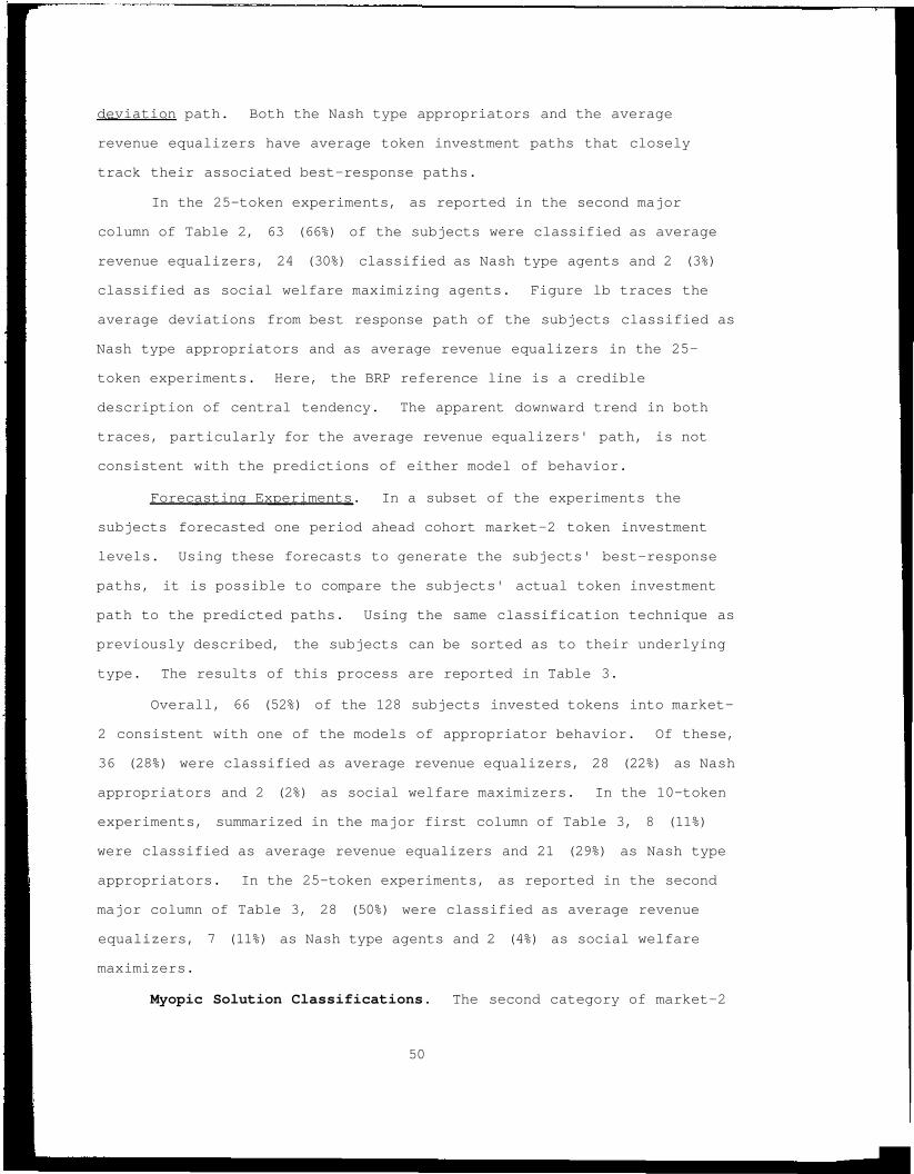
deviation path. Both the Nash type appropriators and the average

revenue equalizers have average token investment paths that closely

track their associated best-response paths.

In the 25-token experiments, as reported in the second major

column of Table 2, 63 (66%) of the subjects were classified as average

revenue equalizers, 24 (30%) classified as Nash type agents and 2 (3%)

classified as social welfare maximizing agents. Figure lb traces the

average deviations from best response path of the subjects classified as

Nash type appropriators and as average revenue equalizers in the 25-

token experiments. Here, the BRP reference line is a credible

description of central tendency. The apparent downward trend in both

traces, particularly for the average revenue equalizers' path, is not

consistent with the predictions of either model of behavior.

Forecasting Experiments. In a subset of the experiments the

subjects forecasted one period ahead cohort market-2 token investment

levels. Using these forecasts to generate the subjects' best-response

paths, it is possible to compare the subjects' actual token investment

path to the predicted paths. Using the same classification technique as

previously described, the subjects can be sorted as to their underlying

type. The results of this process are reported in Table 3.

Overall, 66 (52%) of the 128 subjects invested tokens into market-

2 consistent with one of the models of appropriator behavior. Of these,

36 (28%) were classified as average revenue equalizers, 28 (22%) as Nash

appropriators and 2 (2%) as social welfare maximizers. In the 10-token

experiments, summarized in the major first column of Table 3, 8 (11%)

were classified as average revenue equalizers and 21 (29%) as Nash type

appropriators. In the 25-token experiments, as reported in the second

major column of Table 3, 28 (50%) were classified as average revenue

equalizers, 7 (11%) as Nash type agents and 2 (4%) as social welfare

maximizers.

Myopic Solution Classifications. The second category of market-2

50

token investment involves subjects myopically exploiting the CPR as

predicted by one of the three symmetric solutions, even when the

aggregate symmetric solution is not achieved. To test if a subject's

token investment pattern was significantly different from one of the

predicted symmetric solutions, a two-tailed t-test was used8 at a

significance level of a = 0.05. Using this procedure, all the subjects

were sorted into one of four categories.

1) Average type appropriators, for subjects whose market-2 tokeninvestment patterns were not significantly different from 9tokens, the symmetric average revenue equalizing prediction.

2) Nash type appropriators, for subjects whose market-2 tokeninvestment pattern was not significantly different from 8 tokens,the symmetric Nash equilibrium prediction.

3) Social type appropriators, for subjects whose Market-2 tokeninvestment patterns were not significantly different from 4, 5tokens the social welfare maximizing symmetric solution.

4) None for subjects whose token investment patterns weresignificantly different from the three previous.

The results of this process are reported in Table 4.

Pooled over all experiments, 96 (44%) of the 216 subjects were

classified as following one of the three symmetric solution paths. Of

these, 33 (15%) were classified as following the symmetric average

revenue maximizing solution path, 46 (21%) as following the symmetric

Nash equilibrium token investment path, and 17 (8%) as following the

social welfare maximizing solution.

In the 10-token experiments, summarized in the first major column

of Table 4, 24 (18%) were classified as average revenue equalizers, 34

(25%) as Nash type appropriators and 9 (7%) as social welfare

maximizers. Figure 2a reports the period by period average token

investment of the subjects classified as either average revenue

equalizers, Nash appropriators, or social welfare maximizers. It also

indicates the three symmetric solutions as reference lines where SARE is

8The Wilcoxon test was not used because it tests whether two samplesare drawn from a population with the same underlying distribution. Themyopic solutions are point solutions and not a random sample. The t-testis more appropriate.

51

the symmetric average revenue equalizing solution, SNE is the symmetric

Nash equilibrium and SWO is the symmetric social welfare optimum.

Figure 2a shows how closely the average token investment paths track the

respective symmetric solution path.

The second major column of Table 4 summarizes the results of the

classification process on the 25-token experiments. Of the 80 subjects

who took part in the 25-token experiments, 9 (11%) were classified as

average revenue equalizers, 12 (15%) as Nash appropriators, and 8 (10%)

as social welfare maximizers. Figure 2b reports the average per-period

token investment path of the subjects classified as following one of the

symmetric paths in the 25-token experiments. The token investment paths

in Figure 2b are visibly more erratic than those in Figure 2a. This can

be partially explained by the larger strategy set faced by subjects in

the 25-token experiments.

The perceived differences between the subject classification

results in 25-token and 10-token experiments led to questions on the

effects the different experimental treatments have on subject behavior.

VI. Results: Treatment Effects on Subject Classification

These experiments had three distinct treatments: subject

endowment, subject experience, and forecasting. Subject endowment level

and subject experience level were treatments examined by Walker, Ostrom

and Gardner at the aggregate level. They found that 25-token

experiments tended to have higher market-2 token investment levels than

10-token experiments. They also found that experiments with experienced

subjects tended to have higher market-2 token investment levels than

experiments with inexperienced subjects.

The models assuming objective maximizing agents are mute on the

effects of explicit forecasting or the effects of experience. Further,

endowment levels should impact token investment levels only when the

endowment constraint is binding. That is, the endowment treatment

52

should not impact subject type, only token investment levels. If the

10-token endowment proved binding, then the 25-token experiments should

exhibit higher aggregate token investment levels.

To test for significant treatment effects, the subject type

results generated from the perfect-foresight best-response

classification scheme (reported in Table 2) were used. This data set

was used because it was measurable for all the experiments and

represents an interpretation of objective maximizing agents.

Proportions of subject type were pooled by experiment treatment types.

Then the Z-test for the significance of difference between sample

proportions was used on the target treatment, holding the other

treatments constant.

Endowment Treatment. Table 5 reports the results of this

procedure on the endowment treatment. Each cell in the table reports

the Z-value of the test with the associated p-value in parentheses. As

reported in the first row of Table 5, the 10-token experiments have a

significantly {a = 0.05) lower proportion of average revenue equalizers

than the 25-token experiments, across all treatment conditions. This is

balanced, in the bottom row, by significantly higher proportion

subjects following none of the best response paths. In fact, the 10-

token experiments never report a higher proportion of subjects following

a best-response path for any of the behavior types. The significant

increase in average revenue equalizers in 25-token experiments over 10-

token experiments is consistent with the observation of higher rent

dissipation in 2 5-token experiments reported in Walker, Gardner and

Ostrom (1990), but is inconsistent with the hypothesis that token

endowment should not impact appropriator behavior.

Forecasting Treatment. Table 6 reports the results of the

statistical tests examining the impact of forecasting on subject

behavior. These tests show forecasting has no significant impact on

subject behavior. A curious regularity does appear in the first and

53

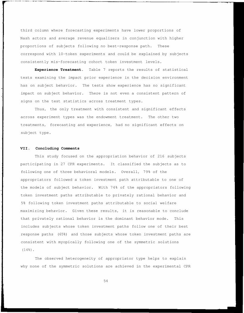
third column where forecasting experiments have lower proportions of

Nash actors and average revenue equalizers in conjunction with higher

proportions of subjects following no best-response path. These

correspond with 10-token experiments and could be explained by subjects

consistently mis-forecasting cohort token investment levels.

Experience Treatment. Table 7 reports the results of statistical

tests examining the impact prior experience in the decision environment

has on subject behavior. The tests show experience has no significant

impact on subject behavior. There is not even a consistent pattern of

signs on the test statistics across treatment types.

Thus, the only treatment with consistent and significant effects

across experiment types was the endowment treatment. The other two

treatments, forecasting and experience, had no significant effects on

subject type.

VII. Concluding Comments

This study focused on the appropriation behavior of 216 subjects

participating in 27 CPR experiments. It classified the subjects as to

following one of three behavioral models. Overall, 79% of the

appropriators followed a token investment path attributable to one of

the models of subject behavior. With 74% of the appropriators following

token investment paths attributable to privately rational behavior and

5% following token investment paths attributable to social welfare

maximizing behavior. Given these results, it is reasonable to conclude

that privately rational behavior is the dominant behavior mode. This

includes subjects whose token investment paths follow one of their best

response paths (65%) and those subjects whose token investment paths are

consistent with myopically following one of the symmetric solutions

(14%).

The observed heterogeneity of appropriator type helps to explain

why none of the symmetric solutions are achieved in the experimental CPR

54

literature. The high proportion of privately rational agents explains

why the experimental CPR literature reports appropriation levels well

above the social optimum.

55

APPENDIX A: Computerized Instructions

This is an experiment in decision making. TheNational Science Foundation has provided funds forconducting this experiment. The instructions aredesigned to inform you of the types of decisionsyou will be making and the results of thosedecisions. All profits you make during theexperiment will be totalled and paid to you inprivacy in cash at the end of the experiment. Ifyou have any questions concerning the instructionsfeel free to raise your hand and one of theexperiment monitors will assist you.

The experiment in which you are participating iscomprised of a sequence of market periods. Ineach market period you will be asked to make aseries of investment decisions. There are also7 other persons in this experiment who will bemaking investment decisions.

Each period you will be allocated an endowment of 25tokens.All other group members also have an endowmentof 2 5 tokens. Total endowment for the group is2 00 tokens.

You will decide each market period how you wish toinvest your endowment between investment opportunitiesThe instructions which follow will describe theinvestment opportunities and the cash return fromeach opportunity.

Your return on investment of tokens in market 1can be explained rather simply. Each token investedin market 1 yields you a return of one unit ofcommodity 1 and each unit of commodity 1 has avalue of $ 0.05.

Thus for example:1) If you invested 3 tokens in market 1 you would

receive 3 units of commodity 1 valued at $ 0.15.

2) If you invested 6 tokens in market 1 you wouldreceive 6 units of commodity 1 valued at $ 0.30.

3) If you invested 9 tokens in market 1 you wouldreceive 9 units of commodity 1 valued at $ 0.45.

IN SUMMARY:A) Each additional token invested in market 1 yields

an additional cash return of $ 0.05.

B) On average you are receiving $ 0.05 per tokeninvested in market 1.

The return on investment of tokens in Market 2 is abit more complicated to explain. In Market 2 thereturn you receive on investments depends on theamount you invest as well as the amount all othersin the group invest.

For example:

56

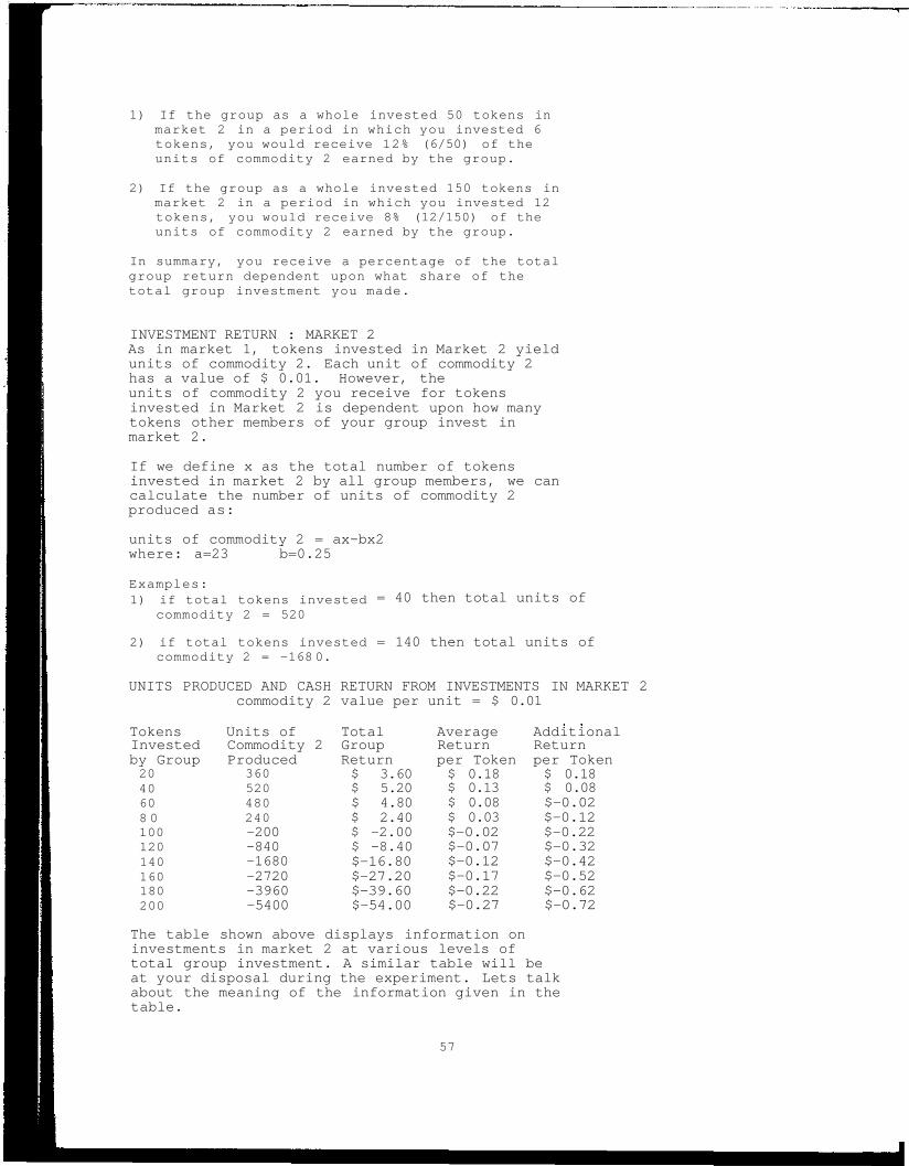
1) If the group as a whole invested 50 tokens inmarket 2 in a period in which you invested 6tokens, you would receive 12% (6/50) of theunits of commodity 2 earned by the group.

2) If the group as a whole invested 150 tokens inmarket 2 in a period in which you invested 12tokens, you would receive 8% (12/150) of theunits of commodity 2 earned by the group.

In summary, you receive a percentage of the totalgroup return dependent upon what share of thetotal group investment you made.

INVESTMENT RETURN : MARKET 2As in market 1, tokens invested in Market 2 yieldunits of commodity 2. Each unit of commodity 2has a value of $ 0.01. However, theunits of commodity 2 you receive for tokensinvested in Market 2 is dependent upon how manytokens other members of your group invest inmarket 2.

If we define x as the total number of tokensinvested in market 2 by all group members, we cancalculate the number of units of commodity 2produced as:

units of commodity 2 = ax-bx2where: a=23 b=0.25

Examples:1) if total tokens invested

commodity 2 = 520

2) if total tokens investedcommodity 2 = -168 0.

= 40 then total units of

= 140 then total units of

UNITS PRODUCED AND CASH RETURN FROM INVESTMENTS IN MARKET 2commodity 2 value per unit = $ 0.01

TokensInvestedby Group2040608 0100120140160180200

Units ofCommodity 2Produced

360520480240-200-840-1680-2720-3960-5400

TotalGroupReturn$ 3.60$ 5.20$ 4.80$ 2.40$ -2.00$ -8.40$-16.80$-27.20$-39.60$-54.00

AverageReturnper Token$ 0.18$ 0.13$ 0.08$ 0.03$-0.02$-0.07$-0.12$-0.17$-0.22$-0.27

AdditionalReturnper Token$ 0.18$ 0.08$-0.02$-0.12$-0.22$-0.32$-0.42$-0.52$-0.62$-0.72

The table shown above displays information oninvestments in market 2 at various levels oftotal group investment. A similar table will beat your disposal during the experiment. Lets talkabout the meaning of the information given in thetable.

57

The first column "Tokens Invested by the Group" givesexample levels of total investment by the group inMarket 2. These are examples to give you a sense ofthe payoff from Market 2 at various levels. Actualreturn from Market 2 will depend on exactly how manytokens your group invests in Market 2.

The second column labeled "Units of Commodity 2 Produced"gives the level of units of commodity 2 produced foreach level of group investment. For example if 100tokens were invested, there would be -200 units ofcommodity 2 produced.

The third column labeled "Total Group Return" displaysthe actual payoff to the entire group for a given levelof group investment. For example, if the group invested100 tokens, the total cash payoff to the group frominvesting in Market 2 would be $-2.00.

The fourth column, labeled "Average Return per Token,"displays the cash value at any level of investment, buton a per token (average) basis. Thus, if the groupinvests 100 tokens, the average return per tokenin Market 2 is $-0.02.

The final column, labeled "Additional Return per TokenInvested'", displays information on the extra value thatis earned from additional tokens invested. Thus, whenthe level of group investment is at 100 tokens,the value of investing additional tokens into Market 2is approximately $-0.22 per token.

1) the return you receive from tokens invested in market 2depends on how many tokens you invest and how many tokensother group members invest in market 2.

2) you will not know how many tokens other group membershave invested in group 2 when you make an investmentdecision in any one period.

3) your individual return from tokens invested inmarket 2 depends on what percentage of the total tokensinvested in market 2 was made by you.

4) By pressing -LAB- during the experiment, you willbe able to have the computer calculate the investmentreturn for MARKET 2 for individual and group decisionslevels chosen by you. Try this now by pressing the-LAB- key on your keyboard.

Yield from Market 2:

Before you make an investment decision during theexperiment, you will have the choice of calling thisoption. By inserting an example level of group investmentand individual investment chosen by you, you can havethe computer compute the yield for Market 2 for theexample you chose.

58

Choose an example for group investment: 70 okChoose an individual investment in Market 2: 10 ok

Units of commodity 2 produced = 3 85Group return = $ 3.8 5Individual return = $ 0.55

Lets take a practice trial to let you get a feel ofwhat it means to actually invest your tokens. Forillustrative purposes only, lets assume you decideto invest 12 of your tokens in market 1 andyour remaining 13 tokens in market 2.

** For example purposes invest 12 tokens in market 1and invest 13 tokens in market 2 **

Number of tokens you wish to invest in Market 1Market 1 investment = 12 ok

Number of tokens you wish to invest in Market 2:Market 2 investment = 13 ok

In this particular example we will assume that othermembers of the group invested a total of 88tokens in the group. This makes total tokens investedin market 2 = 100. Further, this means that youinvested 13% of the tokens in Market 2.

12 units of product 1

MARKET 1:You invested 12 tokens.

This gives you a return ofvalued at $ 0.05 per unit.Total Cash Return = $ 0.60

MARKET 2:

You invested 13 tokens.The total group investment was 100 tokens.

This gives the group a return of -200 units ofproduct 2, valued at $ 0.01 per unit.Total GROUP Cash Return = $-2.00.Your Cash Return = 13% of the total = $-0.26.

This ends the explanation of investment opportunities.During the experiment you will be able to call up asummary of important details regarding the return frominvestments made in the alternative markets.

It is important you fully understand the opportunitiesfor investment. If you have any questions, now is thetime to ask. Just raise you hand.

Otherwise:Press -NEXT- to proceed into the experimentPress -BACK- to reviewPress -DATA- for a summary of investment opportunities

59

ADDITIONAL INSTRUCTIONS

Please read these carefully

At the end of each investment period the computer will display a screenwhich shows the results of the recently completed period. After viewingthe results you can move into the next decision period. Once you haveentered the next decision period, you have many options. These includereviewing the history of decisions, entering a screen which allows youto calculate potential scenarios, and investing in the current period.

Before making your investment decision, you are to make a prediction onwhat you think the total investment of the others will be in Market-2.The total investment of the others will just be the total investment youexpect in market-2 minus what you invest. You will then write thisnumber down beside the appropriate period on the sheet provided for you.

An example: If you intend to invest 5 tokens in market-2 in period 1and you expect the total investment in market-2 will be 40 tokens inperiod 1, then the amount you expect the others to invest in period 1will be 40 - 5 = 35. You would then write 35 in the space besideperiod 1 on the worksheet provided.

At the end of the experiment an investment period will be randomlyselected and the individual whose prediction of the total market-2investment of others is closest to the actual for that period willreceive an additional $3.00. This payment will be divided for ties.

60

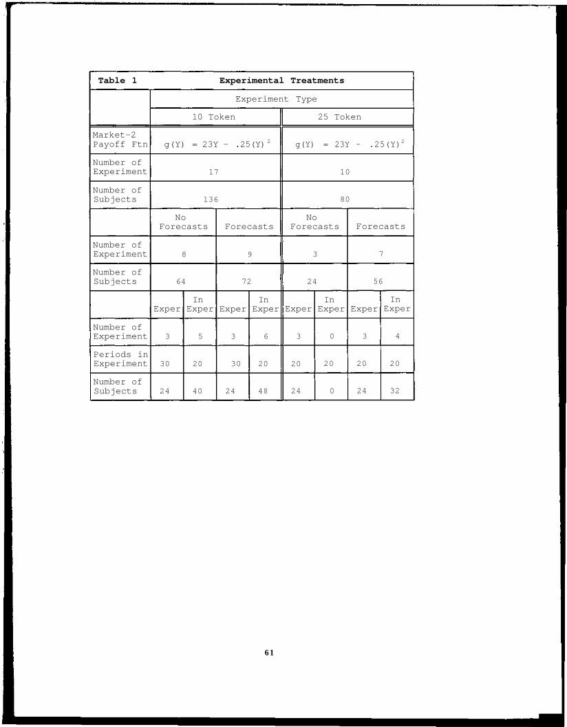
Table 1 Experimental Treatments

Market-2Payoff Ftn

Number ofExperiment

Number ofSubjects

Number ofExperiment

Number ofSubjects

Number ofExperiment

Periods inExperiment

Number ofSubjects

Experiment Type

10 Token

g(Y) = 23Y - .25(Y) 2

17

136

NoForecasts

8

64

Exper

3

30

24

InExper

5

20

40

Forecasts

9

72

Exper

3

30

24

InExper

6

20

48

25 Token

g(Y) = 23Y - .25(Y)2

10

80

NoForecasts

3

24

Exper

3

20

24

InExper

0

20

0

Forecasts

7

56

Exper

3

20

24

InExper

4

20

32

61

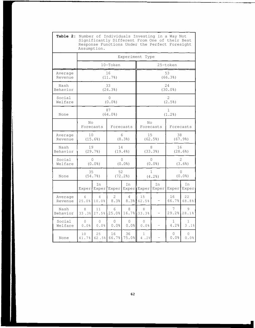
Table 2: Number of Individuals Investing in a Way NotSignificantly Different From One of their BestResponse Functions Under the Perfect ForesightAssumption.

AverageRevenue

NashBehavior

SocialWelfare

None

AverageRevenue

NashBehavior

SocialWelfare

None

AverageRevenue

NashBehavior

SocialWelfare

None

Experiment Type

10-Token

16(11.7%)

33(24.3%)

0(0.0%)

87(64.0%)

NoForecasts

10(15.6%)

19(29.7%)

0(0.0%)

35(54.7%)

Exper

625.0%

833 .3%

00.0%

1041.7%

InExper

410.0%

1127.5%

00.0%

2562 .5%

Forecasts

6(8.3%)

14(19.4%)

0(0.0%)

52(72.2%)

Exper

28.3%

625.0%

00.0%

1666.7%

InExper

48.3%

816.7%

00.0%

3675.0%

25-token

53(66.3%)

24(30.0%)

2(2.5%)

1(1.2%)

NoForecasts

15(62.5%)

8(33.3%)

0(0.0%)

1(4.2%)

Exper

1562.5%

833.3%

00.0%

14 .2%

InExper

-

-

-

-

Forecasts

38(67.9%)

16(28.6%)

2(3.6%)

0(0.0%)

Exper

1666.7%

729.2%

14.2%

00.0%

InExper

2268.8%

928.1%

13 .1%

00.0%

62

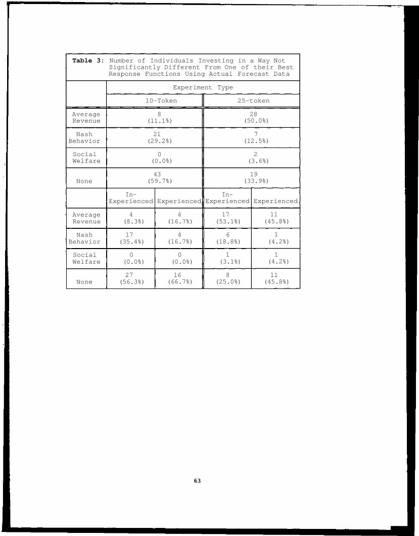
Table 3: Number of Individuals Investing in a Way NotSignificantly Different From One of their BestResponse Functions Using Actual Forecast Data

AverageRevenue

NashBehavior

SocialWelfare

None

AverageRevenue

NashBehavior

SocialWelfare

None

Experiment Type

10-Token

8(11.1%)

21(29.2%)

0(0.0%)

43(59.7%)

In-Experienced

4(8.3%)

17(35.4%)

0(0.0%)

27(56.3%)

Experienced

4(16.7%)

4(16.7%)

0(0.0%)

16(66.7%)

25-token

28(50.0%)

7(12.5%)

2(3.6%)

19(33.9%)

In-Experienced

17(53.1%)

6(18.8%)

1(3.1%)

8(25.0%)

Experienced

11(45.8%)

1(4.2%)

1(4.2%)

11(45.8%)

63

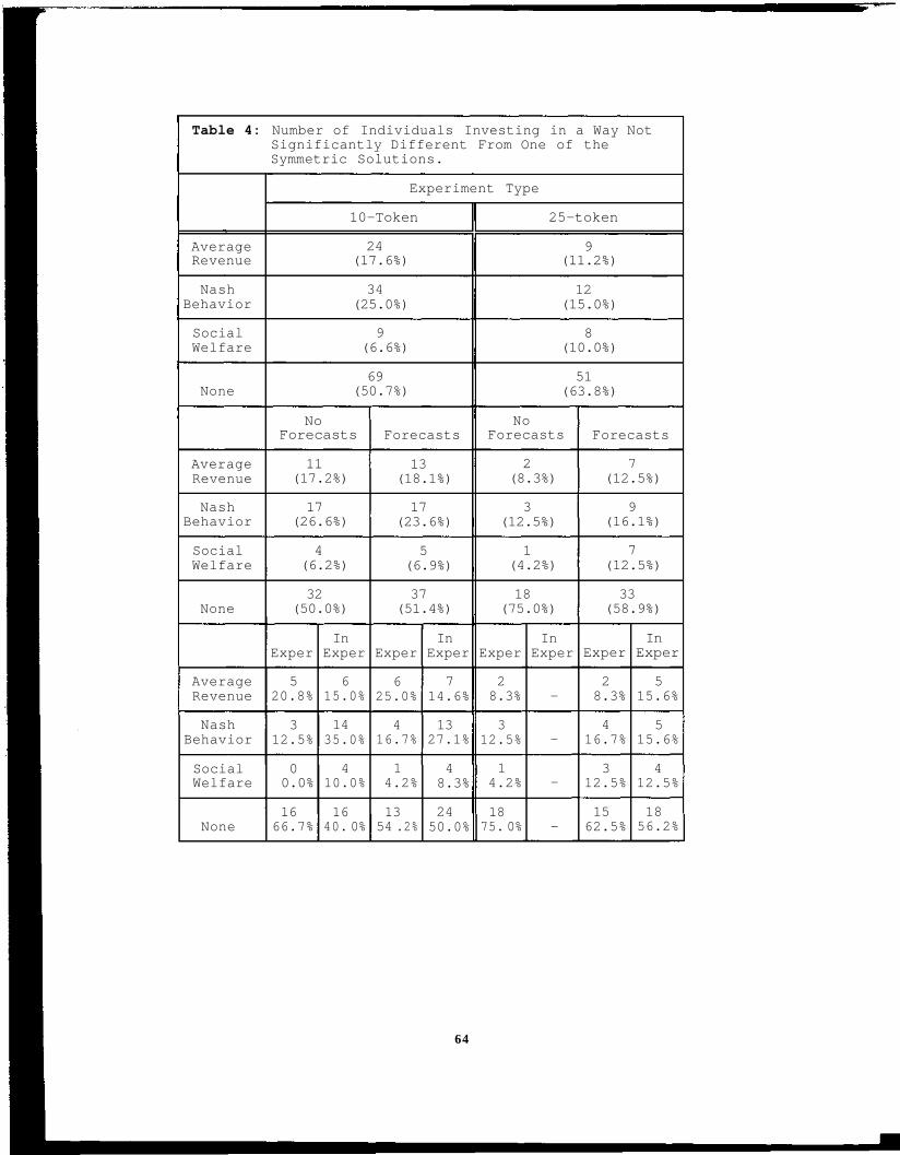
Table 4: Number of Individuals Investing in a Way NotSignificantly Different From One of theSymmetric Solutions.

AverageRevenue

NashBehavior

SocialWelfare

None

AverageRevenue

NashBehavior

SocialWelfare

None

AverageRevenue

NashBehavior

SocialWelfare

None

Experiment Type

10-Token

24(17.6%)

34(25.0%)

9(6.6%)

69(50.7%)

NoForecasts

11(17.2%)

17(26.6%)

4(6.2%)

32(50.0%)

Exper

520.8%

312.5%

00.0%

1666.7%

InExper

615.0%

1435.0%

410.0%

1640. 0%

Forecasts

13(18.1%)

17(23.6%)

5(6.9%)

37(51.4%)

Exper

625.0%

416.7%

14.2%

1354 .2%

InExper

714.6%

1327.1%

48.3%

2450.0%

25-token

9(11.2%)

12(15.0%)

8(10.0%)

51(63.8%)

NoForecasts

2(8.3%)

3(12.5%)

1(4.2%)

18(75.0%)

Exper

28.3%

312.5%

14.2%

1875. 0%

InExper

-

-

-

-

Forecasts

7(12.5%)

9(16.1%)

7(12.5%)

33(58.9%)

Exper

28.3%

416.7%

312.5%

1562.5%

InExper

515.6%

515.6%

412.5%

1856.2%

64

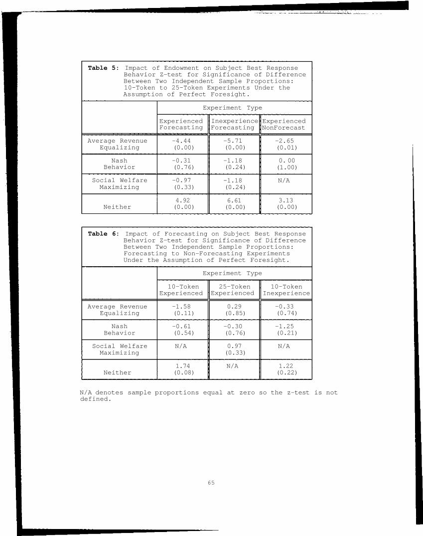
Table 5: Impact of Endowment on Subject Best ResponseBehavior Z-test for Significance of DifferenceBetween Two Independent Sample Proportions:10-Token to 25-Token Experiments Under theAssumption of Perfect Foresight.

Average RevenueEqualizing

NashBehavior

Social WelfareMaximizing

Neither

Experiment Type

ExperiencedForecasting

-4.44(0.00)

-0.31(0.76)

-0.97(0.33)

4.92(0.00)

InexperienceForecasting

-5.71(0.00)

-1.18(0.24)

-1.18(0.24)

6.61(0.00)

ExperiencedNonForecast

-2.65(0.01)

0. 00(1.00)

N/A

3.13(0.00)

Table 6: Impact of Forecasting on Subject Best ResponseBehavior Z-test for Significance of DifferenceBetween Two Independent Sample Proportions:Forecasting to Non-Forecasting ExperimentsUnder the Assumption of Perfect Foresight.

Average RevenueEqualizing

NashBehavior

Social WelfareMaximizing

Neither

Experiment Type

10-TokenExperienced

-1.58(0.11)

-0.61(0.54)

N/A

1.74(0.08)

25-TokenExperienced

0.29(0.85)

-0.30(0.76)

0.97(0.33)

N/A

10-TokenInexperience

-0.33(0.74)

-1.25(0.21)

N/A

1.22(0.22)

N/A denotes sample proportions equal at zero so the z-test is notdefined.

65

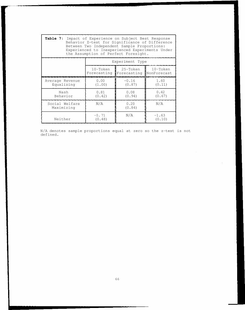
Table 7: Impact of Experience on Subject Best ResponseBehavior Z-test for Significance of DifferenceBetween Two Independent Sample Proportions:Experienced to Inexperienced Experiments Underthe Assumption of Perfect Foresight.

Average RevenueEqualizing

NashBehavior

Social WelfareMaximizing

Neither

Experiment Type

10-TokenForecasting

0.00(1.00)

0.81(0.42)

N/A

-0. 71(0.48)

25-TokenForecasting

-0.16(0.87)

0.08(0.94)

0.20(0.84)

N/A

10-TokenNonForecast

1.60(0.11)

0.42(0.67)

N/A

-1.63(0.10)

N/A denotes sample proportions equal at zero so the z-test is notdefined.

66

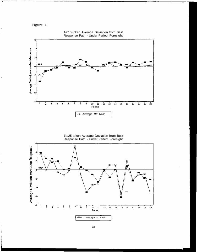
Figure 1

1a:10-token Average Deviation from BestResponse Path - Under Perfect Foresight

10 11 12 13Period

14 15 16 17 18 19 20

- s - Average Nash

1b:25-token Average Deviation from BestResponse Path - Under Perfect Foresight

10 11 12 13 14 15 16 17 18 19 20

---Average -- Nash

6 7

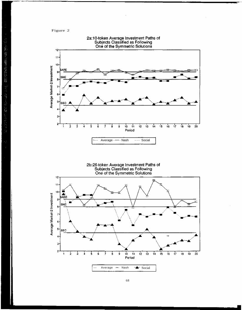
Figure 2

- - - Average - • • - Nash - - - Social

--- Average -••- Nash Social

68

CHAPTER 4

FORECASTING BEHAVIOR IN EXPERIMENTAL COMMON POOL

RESOURCE APPROPRIATION AND PUBLIC GOOD

PROVISION ENVIRONMENTS

I. Introduction

It is not unusual for a decision maker to be in an environment

where outcomes are contingent upon the decision maker's strategy and an

event which reveals itself simultaneously with the decision maker's

strategy choice. Thus, a decision maker selects a strategy given some a

priori belief as to the nature of the event. John Muth (1961) proposed

these forecasts held certain characteristics. In particular, Muth

proposed the subjective probability distribution used by a rational

decision maker to make an informed prediction of a future event is the

same as the objective probability distribution about the realization of

the event itself. This implies that a rational decision maker's

prediction is an efficient and an unbiased estimate of the event. A

competing view of forecasting behavior explicitly models the forecasting

process. In the adaptive model of forecasting behavior, a current

forecast of an event is the old forecast updated after the realization

of the prior event, taking into account forecast error.

Many empirical investigations of the Muthian Rational Expectations

(RE) forecasts have focused on price forecasting. The investigations

include survey-based studies on aggregate price indices (Thies [1986],

Bryan and Gavin [1986], DeLeeuw and Mckelvey [1984] and Gramlich

[1983]) . These studies ask participants to forecast aggregate prices

over time. They find little evidence supporting RE forecasts. There

have also been experimental studies of price forecasting where subjects

forecast prices in experimental markets (Williams [1987], Garner

[1982]). Again, the data are not supportive of RE price forecasts.

69

They do, however, show evidence consistent with adaptive forecasts.

Though the Williams (198 7) market experiments, where subjects

forecast mean prices, were designed to establish a "(non-trivial)

sufficient environmental condition" for RE forecasting, I feel there are

environmental factors which complicated the forecasting task and need to

be addressed. In this type of market environment there is a necessary

position asymmetry between subjects; some are buyers and some sellers.

In addition, there are individual induced valuation asymmetries that

encourage trade by all of the subjects. Given these asymmetries, the

focus of individual buyers and sellers is their intra-period price path

(in attempts to extract a larger share of available buyer/seller

surplus) and not the "mean price." Thus, forecasting the mean price is

ancillary to the task of trading. To address the asymmetry issue a

forecasting environment with a unique symmetric solution and a single

position is needed. In addition, the forecast target needs to be a

primary concern of the participants.

In common pool resource (CPR) appropriation, discussed in Chapter

3, forecasts of cohort appropriation levels are necessary for best

response appropriation. The same is true for the public good provision

problem discussed in Chapter 2.

Walker, Gardner and Ostrom (1990) investigated a series of

repeated play symmetric CPR appropriation experiments. Groups of eight

subjects made appropriation decisions in each of twenty to thirty

repetitions of the CPR environment. The unique, symmetric Nash

equilibrium was never played. An investigation into individual

appropriator behavior in these CPR environments found a limited number

of subjects appropriate in a way consistent with Nash best response

functions (Dudley 1992). A similar lack of convergence to Nash

equilibrium play was observed in the Isaac and Walker (1992) public good

experiments. One explanation for non-Nash behavior is subjects'

inability to form accurate forecasts of cohort appropriation or

70

provision levels; resulting in biased forecasts.

In this study, appropriator forecasting behavior in an

experimental CPR setting with a unique symmetric Nash equilibrium and

provider forecasting behavior in an experimental public good setting are

examined1. The next section gives a brief overview of the experimental

environments in which subject forecasts were made. The results are then

analyzed in section III and concluding comments are made in section IV.

II. Experimental Environment

As, to date, there is little empirical support for the rational

expectations hypothesis. The experimental environments investigated

here, have design characteristics which should not impede RE forecasting

behavior.

The CPR experiments were a supergame consisting of twenty or

thirty repetitions of a one-shot CPR constituent game described in

Chapter 3, Walker Gardner and Ostrom (1990) and Dudley (1992) . Each

subgame had a unique symmetric Nash equilibrium. The only subgame

perfect Nash equilibrium to the supergame consisted of consecutive play

of the subgame Nash equilibrium. Thus, as in Williams (198 7), the

supergame was an operational approximation of a steady state

environment. In this environment the subjects were asked to forecast

cohort investment in the CPR. The public good experiments were a

supergame consisting of 10 repetitions of a one-shot internal Nash

public good constituent game as described in Chapter 2 and Isaac and

Walker (1992). In this environment the subjects were asked to forecast

cohort investment toward the public good.

All the experiments were run on the NovaNET computer network. The

subjects were volunteers from principles of microeconomics courses at

Indiana University. Their earnings were the sum of: 1) the return from

3.-"•These experiments are explained in greater detail in chapters 2 and

71

tokens (generic production units) invested into two experimental

"markets2," 2) $3.00 for showing up on time to the experiment and, 3)

$3.00 for the subject whose forecast error was the smallest in a period

randomly selected at the conclusion of the experiment3. The CPR

experiments had eight subjects and the public good experiments had 4

subjects; each with symmetric payoff and strategy sets.

A total of 2816 forecasts were collected from the subjects in 16

CPR experiments. In 10 of the CPR experiments the subjects were

inexperienced; they had never participated in a CPR experiment before.

In 6 experiments the subjects were experienced volunteers recruited from

the 10 inexperienced experiments. The experienced experiments always

had subjects from more than one of the inexperienced experiments. This

design allows for comparison between forecasts made by novices and

individuals who had experienced the environment and then returned to

participate again. Thus, forecasting can be examined as a time series

through a single experiment as well as comparing forecasts in

experienced runs to inexperienced runs. The experiments are also

differentiated by token endowment. In nine of the experiments, the

subjects had a smaller per-period strategy set of 10 tokens. In the

remaining 7 experiments subjects had a larger per-period strategy set of

25 tokens.

A total of 240 forecasts were collected from the 24 subjects in

the 6 public good forecasting experiments. All of the subjects had

participated in a previous non-forecasting trainer experiment.

2In the CPR experiment the choice is between Market-1 (a privateproductive process) and in Market-2 (a CPR) . In the public goodexperiments the choice is between the Private Exchange (the privateprocess) and the Group Exchange (the public good).

3The reasons for this payoff mechanism are explained in Chapters 2 and3. There was no explicit payment made for forecasts in the 10-token CPRexperiments for reasons explained in Chapter 3.

72

III. The Experimental Results

In both the CPR and public good environments, theory indicates

that income maximizing subjects will seek to maximize their joint return

from the two "markets." As shown in chapters 2 and 3, this yields best

response criteria that are functions of cohort market-2 or group

exchange investment. Thus, subjects have an incentive to forecast cohort

investment levels (YT ). An appropriator's forecast error, in period t,-i

is the difference between observed cohort investment and the forecast,

or

FORECAST ERROR = tYT - tYT.-i -i

Summary of Aggregate Behavior. In these experiments, as is seen

in other CPR and internal Nash public good experiments, the one-shot

Nash equilibrium was never achieved. In the CPR experiments the average

aggregate market-2 investment levels were near those predicted by the

Nash equilibrium4. In addition, as described in Chapter 3, 52% of the

subjects in these experiments followed investment paths not

significantly different from a best-response path. In the public good

experiments, as reported in chapter 2, 45% of the subjects had group

exchange investment paths consistent with one of their best response

paths.

Figure 1 displays a frequency histogram of forecast errors pooled

across all subjects in all the CPR experiments. Figure 2 is a frequency

histogram of forecast errors pooled across all subjects in all of the

public good experiments. The tendency for forecast errors to

concentrate closely around zero implies effort on the part of the

subjects to minimize forecast error.

The distribution of the forecast errors in Figure 1 is skewed to

the right, implying a bias to under estimate cohort market-2

investments; as evidenced by mean = 1.97 > median = 1 > mode = -2.

4For more in depth analysis of these points see Walker, Gardner,Ostrom (1990).

73

Cohort forecast error also falls across a broad range from -51 tokens to

58 tokens with a standard deviation of 12.00 tokens. In addition, the

mean forecast error is significantly different from zero at any

reasonable significance level with

= 8.66.

The distribution of the public good experiment forecast errors in

Figure 2 is skewed to the left, implying a bias to over estimate cohort

group exchange investments; as evidenced by mean = -5.75 < median = -3 <

mode = 2. Cohort forecast error also falls across a broad range from

-148 tokens to 91 tokens with a standard deviation of 33.76 tokens. In

addition, the mean forecast error is significantly different from zero

at any reasonable significance level with t = -2.64.

Analysis of Individual Behavior. Though forecasting behavior has

implications on group outcomes, forecasting is an individual level

behavior. Thus, tests for the RE hypothesis and adaptive forecasting

must be done on the individual level.

The Rational Expectations Hypothesis. A test of the RE hypothesis

comes from Muth's (1961) assertion that "Information is scarce, and the

economic system generally does not waste it." Thus, information

contained in an individual's previous forecasting error is updated into

current forecasts. There should be no residual information from a past

forecast error in a current forecast error. This restriction on

forecasts implies forecast errors should not be serially correlated.

If the restriction is valid then the time series regression equation

(tY

T _

tY

T ) β

0 + β

1(

t - lY

T -

t - 1Y

T ) + t

μ

-i -i -i -i

with the null hypothesis Ho: (Sx = 0 will be accepted.

Table 1 reports the results of the fixed effects panel

regressions. Subjects were pooled by experiment type. First order

serial correlation is rejected in all poolings except the 10 token

inexperienced CPR and Nash-48 public good experiments; lending limited

support to the RE hypothesis. Homogeneity between subjects within

poolings is rejected for each experiment type.

74

The lack of homogeneity across subjects implies potential bias in

the estimates of β. To compensate for the potential bias individual

level regressions were run. As reported in Table 2, at a significance

level (X = 0.05, serial correlation of forecast errors can be rejected

for 87.5% of both the CPR and the public good subjects; reversing the

fixed effects results for the 10 token inexperienced and Nash-48

experiments. Table 2 also reports findings at the 10% and 50%

significance levels indicating the robustness of failing to reject Ho.

These results strongly support the efficient use of information implied

by the RE hypothesis.

The RE hypothesis, also implies that an appropriator's forecast of

cohort investment levels is an unbiased estimate of the realized cohort

investment levels or

YT = Y

T + v.

-i -i

Forecasts of cohort investment levels (YT ) predict the actual cohort-i

investment levels (YT ) up to a random error term with a zero mean (v).-i

This specification can be tested using the time-series regression

equationtY

T = β

o + β

1

tY

T +

tμ

-i -i

with the null hypothesis Ho: (β0, β

1) = (0, 1).

Table 3 reports the results of the fixed effects panel

regressions. The Hypothesis βl = 1 is easily rejected for all

experiment types. The homogeneity across subjects within a pooling is

also rejected.

Because of the lack of homogeneity, the restricted regression

model (βo = 0 , βi = 1) was run for each subject. As shown in Table 4,

with a = 0.05, only 18.8% of the CPR subjects and 33.3% of the public

good subjects have unbiased forecasts. These results do not support

unbiased forecasts as pervasive in the subject pool.

The RE hypothesis suggests both efficient information use and

unbiased forecasts. Those subjects meeting both criteria show evidence

75

of making RE forecasts. The pooled results support efficient use of

information but do not support unbiased forecasts. From the individual

level tests, only 17.8% of the subjects have forecasts consistent with

both criteria. This does not support RE forecasts as descriptive of

individual level forecasting. And, biased forecasts is consistent with

the observed skewed distributions of pooled forecast errors reported in

Figures 1 and 2.

Adaptive Forecasts. Adaptive forecasting behavior implies current

forecasts are updates of prior forecasts from lagged forecast errors.

This type of forecasting, coupled with uncorrelated forecast errors,

implies a current forecast of cohort market-2 token investment (tYT) is

derived from a function that weights lagged one period cohort group

exchange or market-2 investment forecasts (t-1YT ) together with lagged-i

one period forecast error (t-1YT - t-1YT ) . Yielding the adaptive-i -i

specification of

tY

T =

t-1Y

T + β

1 (

t-1YT -

t-1Y

T ) .

-i -i -i

This yields the regression equation

tY

T _

t-1Y

T = β

o + β

1(

t-1Y

T -

t-1Y

T) +

tμ,

-i -i -i

with the null hypothesis Ho: βO = 0 and 0 < β

1 < 1.

Table 5 reports the results from the fixed effects panel

regressions. The hypothesis β1 > 0 and β

1 < 1 is supported for all

experiment types, with β1 ranging from 0.42 to 0.71. Homogeneity across

subjects within experiment type is also accepted. In addition, β0 = 0

is accepted for 72.7% of the CPR subjects and 62.5% of the public good

subjects.

The individual level regressions were run for consistency with the

RE forecasting tests. As shown in Table 6, β1 is significantly less

than one and significantly greater than zero (a = 0.05) for 75.8% of the

CPR subjects and 33.3% of the public good subjects. This is strong

evidence that adaptive learning is a useful model for describing the

subjects' forecasting behavior in the CPR experiments.

76

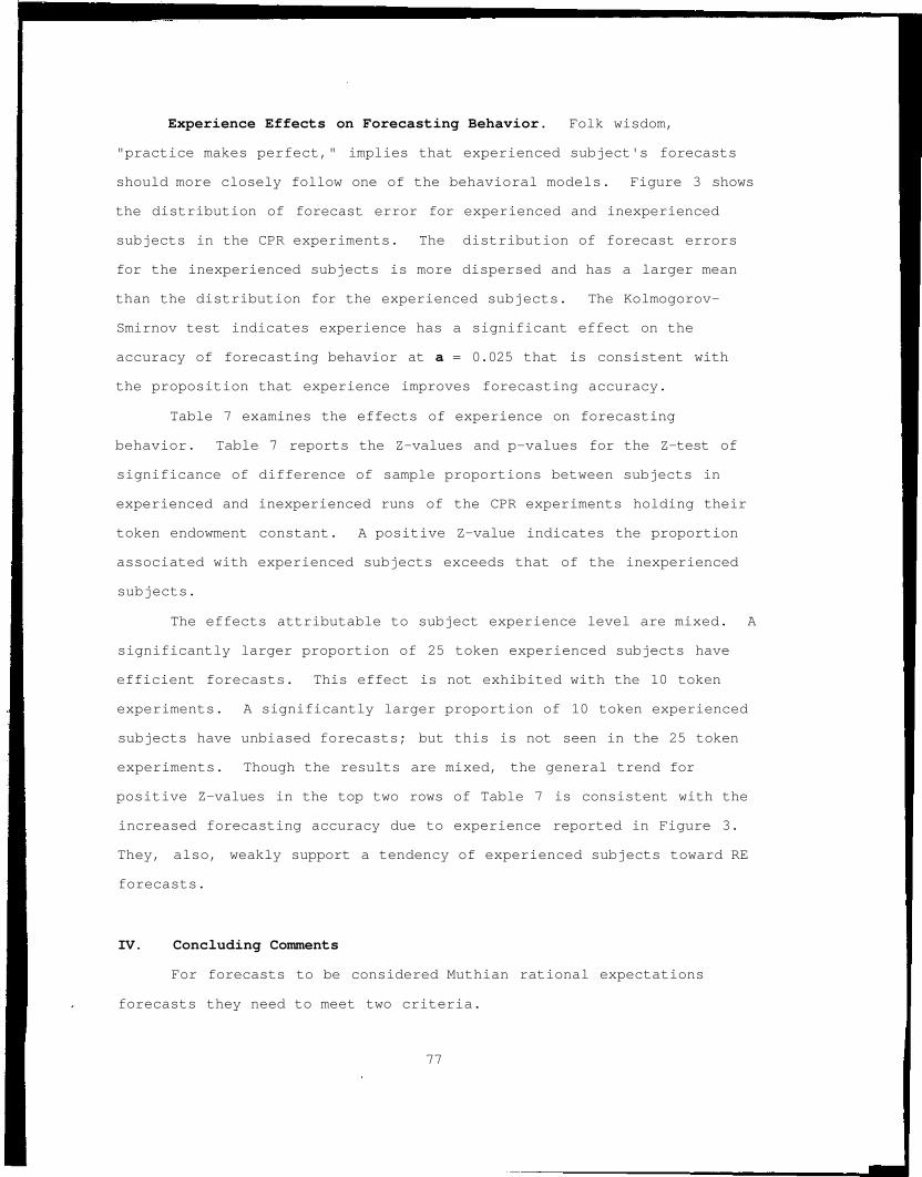
Experience Effects on Forecasting Behavior. Folk wisdom,

"practice makes perfect," implies that experienced subject's forecasts

should more closely follow one of the behavioral models. Figure 3 shows

the distribution of forecast error for experienced and inexperienced

subjects in the CPR experiments. The distribution of forecast errors

for the inexperienced subjects is more dispersed and has a larger mean

than the distribution for the experienced subjects. The Kolmogorov-

Smirnov test indicates experience has a significant effect on the

accuracy of forecasting behavior at a = 0.025 that is consistent with

the proposition that experience improves forecasting accuracy.

Table 7 examines the effects of experience on forecasting

behavior. Table 7 reports the Z-values and p-values for the Z-test of

significance of difference of sample proportions between subjects in

experienced and inexperienced runs of the CPR experiments holding their

token endowment constant. A positive Z-value indicates the proportion

associated with experienced subjects exceeds that of the inexperienced

subjects.

The effects attributable to subject experience level are mixed. A

significantly larger proportion of 25 token experienced subjects have

efficient forecasts. This effect is not exhibited with the 10 token

experiments. A significantly larger proportion of 10 token experienced

subjects have unbiased forecasts; but this is not seen in the 25 token

experiments. Though the results are mixed, the general trend for

positive Z-values in the top two rows of Table 7 is consistent with the

increased forecasting accuracy due to experience reported in Figure 3.

They, also, weakly support a tendency of experienced subjects toward RE

forecasts.

IV. Concluding Comments

For forecasts to be considered Muthian rational expectations

forecasts they need to meet two criteria.

77

1) The efficient use of scarce information, implying no serialcorrelation in forecast errors.

2) A parity between the subjective and the objective probabilitydistributions about the forecast target, implying rationalexpectations forecasts are unbiased estimates of eventrealizations.

Both the fixed effects panels and the individual level regressions

strongly reject serial correlated forecast errors, strongly supporting

efficient information usage. The panel tests reject unbiased forecasts

and this result is strengthened with only 18.8% of the CPR subjects and

33.3% of the public good subjects evidencing unbiased forecasts in the

individual level tests. These results show the rational expectations

hypothesis as a poor description of forecast behavior in these

experimental environments.

There is strong evidence from the panel tests supporting subjects

use adaptive learning in their forecasts. This result is supported by

the individual level tests of the CPR subjects. There is, at best, weak

support by the individual level tests of the public good subjects. As

with other forecasting studies in other environments, adaptive forecasts

are more descriptive of actual forecasts than Muthian rational

expectations forecasts. The dominance of adaptive forecasting over RE

forecasts is mitigated by tests on the effects of experience in the CPR

experiments. These tests show modest evidence that experience increases

RE forecasting.

There is an interesting behavioral difference in forecasting

between the CPR and public good experiments. Subjects tend to under

estimate cohort appropriation in the CPR experiments and tend to over

estimate cohort provision in the public good experiments. This

behavior, in both cases, tends to push subjects away from socially

optimal behavior; due to over optimistic beliefs of cohort investment.

78

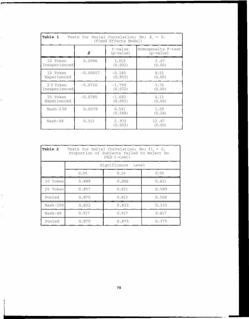
Table 1 Tests for Serial Correlation: Ho: β1 = 0.

(Fixed Effects Model)

10 TokenInexperienced

10 TokenExperienced

2 5 TokenInexperienced

25 TokenExperienced

Nash-2 00

Nash-48

0.0996

-0.00657

-0.0716

-0.0785

0.0579

0.312

t-value(p-value)

3.019(0.002)

-0.185(0.853)

-1.799(0.072)

-1.682(0.093)

0.541(0.588)

2 .972(0.003)

Homogeneity F-test(p-value)

3 .67(0.00)

8.53(0.00)

3.76(0.00)

6.13(0.00)

1.29(0.24)

12 .47(0.00)

Table 2 Tests for Serial Correlation: Ho: fix = 0.

Proportion of Subjects Failed to Reject Ho(OLS t-test)

10 Token

25 Token

Pooled

Nash-200

Nash-48

Pooled

Significance Level

0.05

0.889

0.857

0.875

0.833

0.917

0.875

0.10

0.806

0.821

0.813

0.833

0.917

0.875

0.50

0.431

0.589

0.500

0.333

0.417

0.375

79

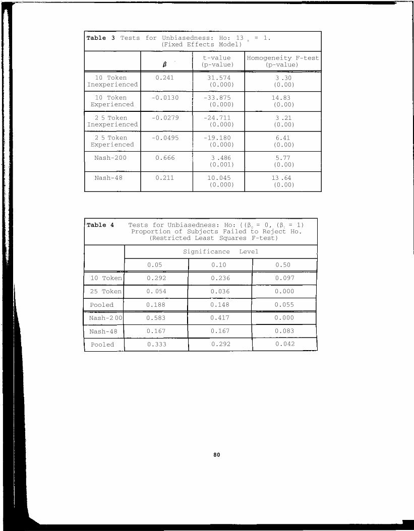
Table 3 Tests for Unbiasedness: Ho: 13 x = 1.

(Fixed Effects Model)

10 TokenInexperienced

10 TokenExperienced

2 5 TokenInexperienced

2 5 TokenExperienced

Nash-200

Nash-48

0.241

-0.0130

-0.0279

-0.0495

0.666

0.211

t-value(p-value)

31.574(0.000)

-33.875(0.000)

-24.711(0.000)

-19.180(0.000)

3 .486(0.001)

10.045(0.000)

Homogeneity F-test(p-value)

3 .30(0.00)

14.83(0.00)

3 .21(0.00)

6.41(0.00)

5.77(0.00)

13 .64(0.00)

Table 4 Tests for Unbiasedness: Ho: {(β0 = 0, (β

1 = 1)

Proportion of Subjects Failed to Reject Ho.(Restricted Least Squares F-test)

10 Token

25 Token

Pooled

Nash-2 00

Nash-48

Pooled

Significance Level

0.05

0.292

0. 054

0.188

0.583

0.167

0.333

0.10

0.236

0.036

0.148

0.417

0.167

0.292

0.50

0.097

0.000

0.055

0.000

0.083

0.042

8 0

Table 5 Tests for Adaptive Forecasts Ho: βo = 0

and 0 < Β < 1. (Fixed Effects Model)

10 TokenInexperienced

10 TokenExperienced

2 5 TokenInexperienced

2 5 TokenExperienced

Nash-200

Nash-48

0.556

0.592

0.523

0.421

0.710

0.571

t-value0i > 00i < 1

23.999-19.181

24.127-16.574

20.789-18.995

14.551-20.039

11.520-4.713

7.579-5.711

p-valuep-value

0.0000.000

0.0000.000

0.0000.000

0.0000.000

0.0000.000

0.0000.000

Proportion

of Subjects

βO = o

0.729

0.750

0.688

0.750

0.833

0.417

Table 6 Test for Adaptive Forecasts. Proportion ofSubjects Meeting the Criteria at SignificanceLevel a = 0.05 (OLS t-tests)

10 Token

2 5 Token

Pooled

Nash-200

Nash-48

Pooled

0 < β1 < 1

0.792

0.714

0.758

0.333

0.333

0.333

βo = 0

0.778

0.865

0.789

1.000

0.917

0.958

00 = 00 < β

1 < 1

0.611

0.571

0.594

0.333

0.250

0.292

8 1

Table 7 Tests for Significance of Experience LevelTreatment Effects on Sample Proportions HoldingToken Endowment Constant. (Data from IndividualLevel Tests)

Non-SeriallyCorrelated Errors

UnbiasedForecasts

AdaptiveForecasts

Significance of DifferenceZ-value(p-value)

10 Token

-0.30(0.764)

2.75(0.006)

-2.22(0.026)

2 5 Token

1. 99(0.047)

0.42(0.674)

0.94(0.272)

82

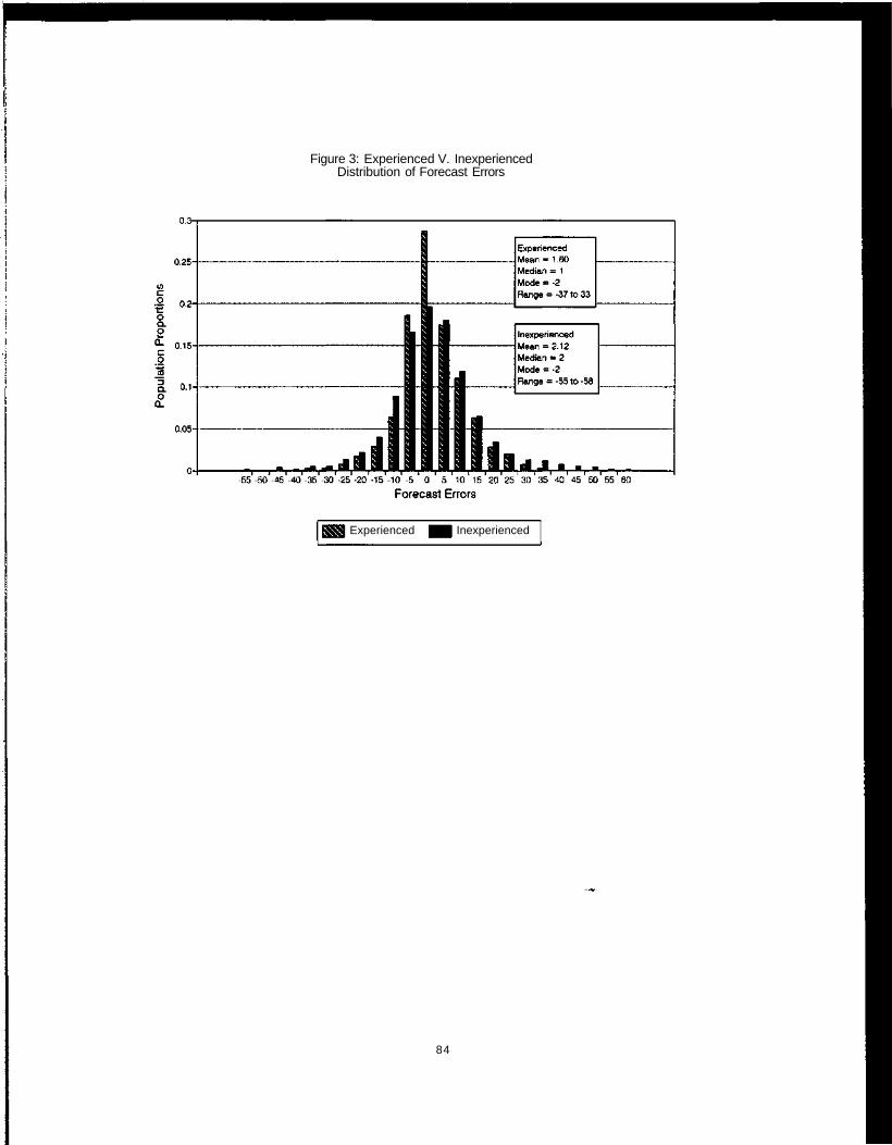
Figure 3: Experienced V. InexperiencedDistribution of Forecast Errors

Experienced Inexperienced

84

CHAPTER 5

CONCLUDING COMMENTS

This study is the synthesis of three interrelated parts. The

first two parts investigated individual level behavior in two different

social dilemma environments. They investigated individual level

provision behavior in an experimental internal-Nash voluntary

contribution public good environment and individual level appropriation

behavior in an experimental limited-access common pool resource

environment. Of primary interest was whether individuals interacted

with purely privately rational motives, ignoring the social costs

imposed by their decisions, or whether they interacted with socially

rational (social welfare maximizing) motives, internalizing the social

costs imposed by their decisions. The third part investigated subject

forecasting behavior in those two environments. Here the focus was on

whether Muthian rational expectations or adaptive forecasting were

descriptive of individual forecasting behavior.

Over all, 75% of the subjects participating in the two

experimental environments exhibited provision or appropriation behavior

consistent with either privately or socially rational motives. The

majority of the subjects, 66% exhibited privately rational behavior and

a minority, 9% exhibited socially rational behavior. This result

implies that private rationality is the dominant behavioral motive in

these two social dilemma environments.

When the results are disaggregated by experiment type an

interesting asymmetry appears. A larger proportion of the public good

experiment subjects exhibit behavior consistent with socially rational

motives1. In addition a larger proportion of CPR experiment subjects

1The test for significance of difference between sample proportionsyields a Z-value of Z = 4.14 and a p-value of p = 0.00.

85

exhibit behavior consistent with privately rational motives2. In the

public good experiments, 43% of the subjects exhibit behavior consistent

with private rationality and 21% of the subjects exhibit behavior

consistent with social rationality. In comparison, 74% of the subjects

in the CPR experiments exhibit behavior consistent with private

rationality and 5% exhibit behavior consistent with social

rationality.3

The difference in observed behavior between the two experimental

environments is surprising because of the structural similarity between

the two environments. Both environments consist of subjects investing

tokens into two "markets"; a "private market" yielding a fixed marginal

return per token and a "group market". The "group market" consisted of

an aggregate production function, that had a negative quadratic form in

both experiment types, and a sharing rule that apportions the aggregate

production between the subjects. In the public good experiments the

sharing rule equally divided the aggregate output between all subjects.

In the CPR experiments the aggregate output was distributed to subjects

in proportion to their token investment in the "group market." The

public good and CPR experiments can also be differentiated by duration

(10 periods in the public good experiments and 2 0 to 3 0 periods in the

CPR experiments) and group size (4 subjects in the public good

experiments and 8 subjects in the CPR experiments. Finally, the two

decision environments were framed differently. The instructions and the

2The test for significance of difference between sample proportionsyields a Z-value of Z = 4.91 and a p-value of p = 0.00.

3A study by Isaac and Walker (1988) suggests that marginal per-capitareturn (MPCR) and not group size induces behavioral change in public goodexperiments. In the public good experiments in this study, the MPCR wasgroup investment dependent and not fixed. The MPCR is not a well definedconcept in the CPR experiments because a subject's share of aggregateoutput is not fixed. Thus, the MPCR's influence is not measurable inthese experiments.

86

decision environment of the public good experiments were more group

oriented.4

The impact of the sharing rule on participant behavior needs to be

investigated more closely. Experiments holding group size, duration and

aggregate production function constant, varying only the sharing rule

need to be run. If the result that an equal share rule results in

greater socially rational behavior in social dilemma environments holds

under a more controlled test, it implies the counter intuitive argument

that institutionally transforming CPRs into public goods (collectivizing

CPRs) may have social welfare enhancing effects.

The final section of this study examined forecasting behavior in

the CPR and public good environments. Over all, adaptive forecasting

was more descriptive of subject forecasts than Muthian rational

expectations (RE). In the CPR experiments, there was some evidence

suggesting experienced subjects' forecasts had increased RE

characteristics. In addition, tests on forecast errors suggested CPR

subjects tended to under estimate cohort appropriation and public good

subjects tended to over estimate cohort provision. In a sense, it seems

that in these two environments, subjects believe their cohorts are

bigger "suckers" than they really are. In both cases, these beliefs

tend to push rational (objective maximizing) subjects away from the

social optimum; regardless of whether they are socially rational or

privately rational. In the public good experiments, over estimated

cohort group exchange investments induce lower private or social best

responses. In the CPR experiments, under estimated cohort market-2

investments induce higher best responses.

This forecasting bias can drive outcomes beyond a subject's target

outcome. Periodically the impact due to forecast bias will result in an

outcome which causes subjects to significantly reevaluate their current

4To see these differences read the computerized instructions in theappendices of chapter 2 and 3.

87

investment strategy. This adjustment will be evidenced by a pulse in

the outcome towards the social optimum. This pulsing behavior is

consistent across the CPR experiments. This dynamic may be one of the

roots of the pulsing aggregate investment behavior in these CPR

experiments.

88

References

Bell, Frederick, "Technological Externalities and Common Property-Resources: An Empirical Study of the U.S. Lobster Industry",Journal of Political Economy, v.80 p.148-158 (1972)

Bresnahan, "Duopoly Models With Consistent Conjectures", AmericanEconomic Review, v.71 p.934-945 (1981)

Bryan, Michael F. and William T. Gavin, "Models of InflationExpectations Formation: A comparison of Household and EconomisrForecasts" Journal of Money, Credit, and Banking v.18 p.539-544(1986)

Clark, "Restricted Access to Common-Property Fishery Resources: A GameTheoretic Analysis" in Dynamic Optimization and MathematicalEconomics p.117-132 Plenum, New York (1980)

Cornes, Richard and Todd Sandier, The Theory of Externalities, PublicGoods, and Club Goods Cambridge University Press, London/New York(1986)

Dawes, Robin, "Social Dilemmas" Annual Review of Psychology v.31 p.16 9-193 (1980)

De Leeuw, Frank and Michael J. McKelvey "Price Expectations of BusinessFirms: Bias in the Short and Long Run" The American EconomicReview v.74 p.99-110 (1984)

Dudley, Dean, "Individual Choice in a Common Pool Resource Environment:An Experimental Analysis" Presented at the Midwest EconomicsAssociation meetings, Chicago, March (1992)

Dwyer, Gerald, Arlington Williams and Raymond Battalio, "Tests ofRational Expectations in a Stark Setting" forthcoming EconomicJournal (1993)

Gardner, Roy and Elinor Ostrom, "Rules and Games" Public Choice (1990)

Gardner, Roy, Elinor Ostrom and James Walker, "The Nature of Common-PoolResource Problems" Rationality and Society v.2 p.335-358 (1990)

Garner, Alan, "Experimental Evidence on the Rationality of IntuitiveForecasts" Research in Experimental Economics v.2, edited byVernon Smith, Greenwich: J.A.I. Press, p.155-173 (1982)

Gordon, H. Scott, "The Economic Theory of a Common Property Resource:The Fishery" Journal of Political Economy v.62 p.124-142 (1954)

Gramlich, Edward M. "Models of Inflation Expectations Formation: AComparison of Household and Economist Forecasts" Journal of Money,Credit, and Banking v.15 p.155-173 (1983)

Hogg, Robert and Allen Craig, Introduction to Mathematical Statistics4th Edition, Macmillan Publishing Co., Inc., New York/London(1978)

Isaac, Mark, James Walker and Susan Thomas, "Divergent Evidence on FreeRiding: An Experimental Examination of Possible Explanations"Public Choice v.43 p.113-149 (1984)

89

Isaac, Mark, Kenneth McCue and Charles Plott, "Public Goods Provisionin an Experimental Environment" Journal of Public Economics v.26p.51-74 (1985)

Isaac, Mark and James Walker, "Group Size Effects in Public GoodsProvision: The Voluntary Contribution Mechanism" Quarterly Journalof Economics February p.179-199 (1988)

Isaac, Mark and James Walker, "Communication and Free-Riding Behavior:The Voluntary Contribution Mechanism" Economic Inquiry v.26 p.585-608 (1988b)

Isaac, Mark and James Walker "Nash as an Organizing Principle in theVoluntary Contribution of Public Goods" Mimeo, Indiana University,October 7 (1992)

Kalai, Ehud and Ehud Lehrer, "Rational Learning Leads to NashEquilibrium" Discussion Paper #895, The Center for MathematicalStudies in Economics and Management, Northwestern University,March (1990)

Kalai, Ehud and Ehud Lehrer, "Subjective Equilibrium in Repeated Games"Discussion Paper #981, The Center for Mathematical Studies inEconomics and Management, Northwestern University, February (1992)

Kim, Oliver and Mark Walker, "The Free Rider Problem: ExperimentalEvidence" Public Choice v.43 p.3-24 (1984)

Lehmann, L. and H. D'Abera Nonparametries: Statistical Methods Based onRanks Holden-Day, Inc. Oakland (1975)

Lovell, Micheal C. "Tests of the Rational Expectations Hypothesis" TheAmerican Economic Review v.76 p.110-124 (1986)

Mason, Charles F., Todd Sandier and Richard Cornes, "Expectations, theCommons, and Optimal Group Size"Journal of Environmental Economics and Management v.15 p.99-110(1988)

Messick, David and Carol McClelland, "Social Traps and Temporal Traps"Personality and Social Psychology Bulletin v.9 p.105-110 (1983)

Muth, John, "Rational Expectations and the Theory of Price Movements"Econometrica v.29 p.315-335 (1961)

Ostrom, Elinor, Governing the Commons: The Evolution of Institutionsfor Collective Action Cambridge University Press, London/New York(1990)

Ostrom, Elinor, Roy Gardner and James Walker, "Covenants With andWithout a Sword: Self Governance is Possible" American PoliticalScience Review v.86 p.1-14 (1992)

Perry, Martin, "Oligopoly and Consistent Conjectural Variations" BellJournal of Economics v.13 p.197-205 (1982)

Samuelson, Paul A. "The Pure Theory of Public Expenditure" Review ofEconomics and Statistics v.36 p.387-389 (1954)

Samuelson, Paul A. "A Diagrammatic Exposition of a Theory of PublicExpenditure" Review of Economics and Statistics v.37 p.350-356(1955)

90

Schmalensee, Richard "An Experimental Study of Expectation Formation"Econometrica v.44 p.17-41 (1976)

Smith, Vernon, Gerry Suchanek and Arlington Williams, "Bubbles, Crashesand Endogenous Expectations in Experimental Spot Asset Markets"Econometrica v.56 p.1119-1151 (1988)

Thies, Clifford F. "Business Price Expectations 1947 - 83" Journal ofMoney, Credit , and Banking v.18 p.336-354 (1986)

Walker, James, Roy Gardner and Elinor Ostrom, "Rent Dissipation in aLimited-Access Common-Pool Resource: Experimental Evidence"Journal of Environmental Economics and Management v.19 p.203-211(1990)

Williams, Arlington, "The Formation of Price Forecasts in ExperimentalMarkets" The Journal of Money, Credit, and Banking v.19 p.1-17(1987)

91

CURRICULUM VITAE

DEAN DAVID DUDLEY

HOME ADDRESS299 Y StreetNew Windsor, NY 12253(914) 567-6069

FIELDS OF SPECIALIZATIONPolitical EconomyPublic FinanceIndustrial Organization

DISSERTATION

Department of Social ScienceUnited States Military AcademyWest Point, NY 10996(914) 938-2898

PERSONALBirthdate: 28 may 1958Marital Status: Married, five children

ESSAYS ON INDIVIDUAL BEHAVIOR IN SOCIAL DILEMMA ENVIRONMENTS:AN EXPERIMENTAL ANALYSIS

In this study a series of computer assisted experimental Common Pool Resource and VoluntaryContribution Public Goods environments are used to collect data on and investigate the individualchoices made by subjects. Given a separation between privately rational and socially optimal strategies,this thesis studies how the competing theories of human behavior hold against the choices made byindividuals in these environments. It also studies how one-period-ahead individual forecasting behaviorconverges to rational expectations forecasts. Information on individuals' choices and forecastingbehavior should lead to more effective policy formation with respect to social dilemma environments.

Chairman: Professor James Walker, Acting Director of the Workshop in Political Theory And PolicyAnalysis, Indiana University, Bloomington, In

EDUCATIONPh.D. Candidate, Economics, Indiana University, Bloomington, InB.A., Economics, Eastern Washington University, Cheney, Wa, 1986

TEACHING EXPERIENCEAssistant Professor, Dept. of Social Science, United States Military Academy, West Point, NY. August1993 to Present.

Associate instructor, Dept. of Economics, Indiana University, Bloomington, In. August 1990 to July1992 (five semesters). Course Taught: E201 Introduction to Microeconomics.

PAPER PRESENTATIONS"Forecasting Behavior in Experimental Common Pool Resource Appropriation and Public GoodProvision Environments" Seminar, Dept. of Soc. Sci. USMA, West Point, NY, August 1993.

"Individual Choice in a Common Pool Resource Environment: An Experimental Analysis" Presented atthe Mid-West Economics Association meetings. Chicago, II, March 1992.

"Individual Behavior in an Experimental CPR Environment," paper presented at the Mini-Conference ofthe Workshop in Political Theory and Policy Analysis, Indiana University, Bloomington, In., May 1989.

"Exciudability: A Composite Symptom of the Institution of Exchange and the Nature of the Resource,"paper presented at the Mini-Conference of fhe Workshop in Political Theory and Policy Analvsis.Indiana University, Bloomington, In., Dec 1988.

RESEARCH POSITIONSVisiting Research Associate to the Workshop in Political Theory and Policy Analysis, IndianaUniversity, Bloomington In, Aug. 1992 to Aug. 1993.

Research Assistant to the Workshop in Political Theory and Policy Analysis, Common PropertyResource project, May 1991 to August 1991.

Research Assistant to Professor David Wildasen, Project on Differential Net Social Security Benefitswith Mobile Labor in the EEC, August 1990.

Research Assistant to the Workshop in Political Theory and Policy Analysis, Head of experimentalcomputer lab for Committee Voting project, August 1989 to August 1990.

Research Assistant to the Workshop in Political Theory and Policy Analysis, Common PropertyResource project, August 1988 to August 1989.

PROFESSIONAL MEMBERSHIPSAmerican Economic Association (student member)MidWest Economics Association

REFERENCESAssistant Professor Steven HackettProfessor Roy GardnerProfessor James Walker,

Acting Director of the Workshop inPolitical Theory and Policy Analysis.

Professor Arlington Williams

Department of EconomicsBallantine Hall 901

Indiana UniversityBloomington, In 47405(812) 855-1021

Distinguished Professor Elinor Ostrom,Co-director of the Workshop inPolitical Theory and Policy Analysis,Arthur F. Bentley Professor In Political Science.

Workshop in Political Theory and PolicyIndiana University513 North ParkBloomington, In 47405(812) 855-0441