Essays on Child Development in Developing Countries

A Dissertation SUBMITTED TO THE FACULTY OF

UNIVERSITY OF MINNESOTA BY

Sarah Davidson Humpage

IN PARTIAL FULFILLMENT OF THE REQUIREMENTS FOR THE DEGREE OF

DOCTOR OF PHILOSOPHY

Paul W. Glewwe

August 2013

© Sarah Humpage 2013

i

Acknowledgments I am grateful for valuable feedback and guidance from Paul Glewwe and for several years of excellent academic advising. The members of my thesis committee, Elizabeth Davis, Deborah Levison and Judy Temple, have provided excellent comments on this work throughout the entire process. Colleagues Amy Damon, Qihui Chen, Kristine West, Daolu Cai, Nicolas Bottan and Irma Arteaga have also provided excellent comments for which I am grateful. Outside of the university, Julian Cristia and Matias Busso have been important advisers for me, providing valuable advice and guidance. The research in all three papers was made possible with financial support from the Inter-American Development Bank. The Center for International Food and Agricultural Policy at the University of Minnesota also provided generous financial support for the research in Peru. The work in Guatemala would not have been possible without the instrumental support of Dr. José Rodas or Dr. Cristina Maldonado. Julian Cristia and Matias Busso had leadership roles in designing the experiment, and coordinating the fieldwork and provided extensive input for the analysis and advice on the chapter. I am also grateful to Stuart Speedie at the University of Minnesota’s Institute for Health Informatics, participants in the American Medical Informatics Association’s 2011 Doctoral Consortium, and participants in the University of Minnesota’s Dissertation Seminar and Trade and Development Seminar, the 2013 Midwest Economics Association meetings and the 2013 Midwest International Economic Development Conference for their valuable comments on the Guatemala paper. Julian Cristia also played an essential role in the research in Peru, supporting the fieldwork as well as the analysis. Carmen Alvarez, Roberto Bustamante, Hellen Ramirez and Guisella Jimenez provided essential support for the fieldwork. Horacio Álvarez provided valuable leadership and support on the Costa Rica project. Personally, I would like to recognize the support of Tony Liuzzi, Carol, Steve and Amanda Humpage and my extended family. My nephew, Will Masanz, makes me appreciate the richness of early childhood every day. My classmates, especially Charlotte Tuttle and Kristine West, made graduate school infinitely more pleasant and rewarding.

ii

Dedication To my grandpa, Charles Davidson, who, along with my parents, showed me the joys of learning, and inspired me to care about the causes and consequences of poverty.

To all the participants in this research, who graciously shared their time and thoughts to make this work possible.

iii

Abstract

This dissertation presents the results of three field experiments implemented to

evaluate the effectiveness of strategies to improve the health or education of

children in developing countries. In Guatemala, community health workers at

randomly selected clinics were given patient tracking lists to improve their ability to

remind parents when their children were due for a vaccine; this is found to

significantly increase children’s likelihood of having all recommended vaccines. This

strategy is particularly effective for older children. In Peru, a teacher training

program is found to have no effect on how frequently children use their computers

through the One Laptop Per Child program. In Costa Rica, learning English as a

foreign language using one software program is found to be significantly more

effective than studying with a teacher, or with a different software program,

confirming the heterogeneity of effects of educational technology.

iv

Table of Contents

List of Tables v List of Figures vii Abbreviations viii Chapter 1: Introduction 1 Chapter 2: Did You Get Your Shots? Experimental Evidence on the Role of

Reminders in Guatemala 5 Chapter 3: Teacher Training and the Use of Technology in the Classroom:

Experimental Evidence from Primary Schools in Rural Peru 47 Chapter 4: Teachers’ Helpers: Experimental Evidence on Computers for English

Language Learning in Costa Rican Primary Schools 102 Chapter 5: Conclusion 146 Bibliography 150 Appendix 159

v

List of Tables

Tables for Chapter 2 Table 2.1: Health and Well-being in Guatemala 38 Table 2.2: Coverage, Delay by Vaccine 39 Table 2.3: Access to PEC Services 40 Table 2.4: Parent Perspectives on Vaccination 41 Table 2.5: Sample 41 Table 2.6: Data management by treatment group from endline survey 42 Table 2.7: Treatment Effects on Complete Vaccination by Group 43 Table 2.8: ITT, LATE estimates of treatment on delayed vaccination (in days) 44 Table 2.9: Survival Analysis for Vaccines at 18 and 48 months 45 Table 2.10: Cost Estimates 46 Tables for Chapter 3 Table 3.1: Learning Objectives of PSPP 86 Table 3.2: Sample 87 Table 3.3: Balance 88 Table 3.4: Teacher Training on OLPC Laptops 89 Table 3.5: Teacher Skills, Behavior and Use of Laptops at Trainers’ First

and Second Visit 90 Table 3.6: Teacher-Reported Barriers to Use 91 Table 3.7: Teacher Computer Use, XO Knowledge & Opinions 92 Table 3.8: Student PC Access, XO Opinions 93 Table 3.9: Use of the XO Laptops According to Survey Data 94 Table 3.10: Use of the XO Laptops by Computer Logs 95 Table 3.11: Type of Use of the XO Laptops by Computer Logs 96 Table 3.12: Effects on Math Scores and Verbal Fluency 97 Table 3.13: Effects by Teacher Age 98 Table 3.14: Effects by Teacher Education 98 Table 3.15: Effects by Student Gender 99 Table 3.16: Effects by Grade 99 Tables for Chapter 4 Table 4.1: Estimates from 1990-2010 of Effects of Computer Use

on Test Scores 130 Table 4.2: Baseline Characteristics and Test Scores 130 Table 4.3: Attrition Rates by Treatment Group 131 Table 4.4: Baseline Characteristics by Treatment Group, Retained Samples 131 Table 4.5: Unadjusted Test Scores by Group, all Time Periods 132 Table 4.6a: Treatment Effects – DynEd vs. Control 133 Table 4.6b: Treatment Effects – Imagine Learning vs. Control 134 Table 4.6c: Treatment Effects – DynEd vs. Imagine Learning 135 Table 4.7a: Effects of DynEd vs. Control for Low-Scoring Schools 136 Table 4.7b: Effects of Imagine Learning vs. Control for Low-Scoring Schools 137

vi

Table 4.7c: Effects of DynEd vs. Imagine Learning for Low-Scoring Schools 138 Table 4.8a: Effects of DynEd vs. Control for Low-Scoring Students 139 Table 4.8b: Effects of Imagine Learning vs. Control for Low-Scoring Students 140 Table 4.8c: Effects of DynEd vs. Imagine for Low-Scoring Students 141 Table 4.9a: Effects of DynEd vs. Control by Gender 142 Table 4.9b: Effects of Imagine Learning vs. Control by Gender 143 Table 4.9c: Effects of DynEd vs. Imagine Learning for Low-Performing Schools 144

vii

List of Figures

Figure 3.1: Photos from the Training 100 Figure 3.2: XO Use in the Last Week by Treatment Group 101

viii

List of Abbreviations

ATE: Average treatment effect ATT: Average treatment effect on the treated CCT: Conditional cash transfer CHW: Community health worker DIGETE: General Office for Educational Technology (Dirección General de

Tecnologías Educativas) DPT: Diphtheria, pertussis and tetanus vaccine EILE: Enseñanza del Inglés como Lengua Extranjera (English as a Foreign

Language Teaching) IDB: Inter-American Development Bank INA: National Learning Institute (Instituto Nacional de Aprendizaje) INEC: National Statistics and Census Institute (Instituto Nacional de

Estadísticas y Censos) ITT: Intent to treat LATE: Local average treatment effect LF: List facilitator MDGs: Millennium Development Goals MEP: Ministry of Public Education (Ministerio de Educación Pública) MMR: Measles, mumps and rubella vaccine NGO: Non-governmental organization OLPC: One Laptop Per Child PEC: Coverage Extension Program (Programa de Extensión de Cobertura) PSPP: Pedagogical Support Pilot Program PTL: Patient tracking list SERCE: Second Regional Comparative and Explanatory Study UNESCO: United Nations Educational, Scientific and Cultural Organization UNICEF: United Nations Children’s Fund WHO: World Health Organization

1

Chapter 1: Introduction

2

Theodore Schultz was one of the first economists to draw attention to the critical

role of human capital in economic development in his 1960 presidential address to

the American Economic Association. Schultz argued that a healthy, well-educated

work force stimulates economic growth (1961). In the decades since Schultz’s 1960

speech, investments in human capital have grown at a dramatic pace. Whereas in

1960, 55% of the population age 15 and over in developing countries had never

been to school, by 2010, this had fallen to 17% (Perkins et al., 2013). From 1960 to

2008, life expectancy rose dramatically from 46 years to 68 years in low and middle-

income countries (World Bank, 2013).

These dramatic improvements in human capital in the developing world may

be seen as the consequence, at least in part, of a policy focus on these issues among

governments and international aid organizations. Five of the United Nations’ eight

Millennium Development Goals (MDGs) focus on improving health or education:

achieving universal primary education; reducing child mortality; improving

maternal health; combating HIV/AIDS, malaria and other diseases; and eradicating

extreme poverty and hunger.

Despite these dramatic improvements in health and education, more work

remains to be done to improve children’s access to basic health care and education

around the world. Over one million children die from vaccine preventable disease

every year (World Health Organization and UNICEF, 2012a). Ten percent of primary

school-aged children were out of school in 2011, and 123 million youth aged 15-24

lack basic reading and writing skills (United Nations, 2013).

The 23 members of the Development Assistance Committee contributed $134

3

billion in development aid in 2011 alone, partly to support countries in their efforts

to achieve the MDGs and other development objectives (OECD, 2013). Yet financial

commitments to development will not be sufficient to sustain improvements in

health and education. For policy-makers in governments and in international aid

organizations to spend their finite financial and other resources efficiently, they will

benefit from reliable information on which programs are most effective in reaching

their objectives. Banerjee and He write argue that policy-makers are long on ideas,

but short on reliable information about what works (2003). Mullainathan points out

that it is challenging for policy-makers and others to obtain unbiased information on

program effectiveness, as many evaluations conducted by implementing agencies

may be biased toward finding effects (2005). Esther Duflo, an economist well-

known for her role in popularizing the use of randomized experiments in

development economics, has argued that the systematic use of randomized

evaluations may contribute to development effectiveness by generating more

reliable estimates of program effectiveness (2004).

This dissertation contributes to the growing body of research on what works

in health and education in developing countries, presenting research from

randomized evaluations conducted in three Latin American countries. Original data

were collected for each essay.

Part of the appeal of randomized experiments is the simplicity with which the

analyst can estimate the causal effect of a program or policy. As is discussed in

greater detail in Chapter 2, when an experiment is implemented properly, a

program’s effect may be estimated simply by comparing means observed in the

4

treatment and comparison groups. On the ground, however, complications are likely

to arise (Barrett and Carter, 2010). In the experiment described in Chapter 2, only

64% of community health workers at clinics assigned to the treatment group

received the treatment, while 14% of community health workers in the control

group indicated that they did. In this case, comparing mean outcomes in the

treatment and comparison groups yields an estimate of the intent to treat effect

rather than the average treatment effect. In an experiment in Costa Rica, the field

team applied the criteria for inclusion inconsistently for the control and treatment

groups, introducing systematic differences among groups. Because of complications

like these, the analysis of randomized evaluations is often less straightforward than

in the ideal case. Several econometric methods are used here that allow for the

estimation of causal effects in spite of these complications.

This dissertation is organized as follows. Chapter 2 presents the results of a

field experiment in Guatemala that estimates the effect of distributing patient

tracking lists to community health workers on the probability of children having all

vaccines recommended for their age. Chapter 3 presents analysis of the impact of

providing teacher training on how teachers and students use the laptops distributed

through the One Laptop Per Child program. Chapter 4 describes the effectiveness of

using computers to teach children English as a foreign language in Costa Rica.

Finally, Chapter 5 concludes.

5

Chapter 2:

Did You Get Your Shots?

Experimental Evidence on the Role of Reminders

From Rural Guatemala

6

1. Introduction

Why do millions of children still fail to receive their recommended vaccines around

the world despite the fact that vaccination is one of the most cost-effective strategies

to reduce child mortality? The global rate of child mortality has declined

dramatically in recent years, from 87 deaths before age five per 1,000 live births in

1990 to 51 in 2011 (UNICEF, 2012), yet child mortality must drop at an even faster

rate, however, to meet the Millennium Development Goal of reducing child mortality

by two thirds by 2015 (Table 2.1 provides descriptive statistics on health and well-

being in Guatemala.). Vaccination may play a key role in achieving this objective, as

it is one of the most cost-effective strategies for improving child survival (Bloom et

al., 2005). Although coverage of routine vaccination has improved dramatically

around the world in the last forty years, the World Health Organization estimates

that more than 19 million children worldwide did not receive their recommended

vaccines in 2010 (World Health Organization and UNICEF, 2012a). As a result, over

1.4 million children die of vaccine-preventable disease every year, representing

29% of all child deaths before age five. A challenge for the public health community

today is to identify strategies to reach those who remain unvaccinated and to follow

up with the children who receive some vaccines but fail to receive them all.

This paper tests one such strategy, presenting the results of a field

experiment that introduces exogenous variation in the probability that families in

rural Guatemala receive personal reminders from community health workers to

notify them when their child is due to receive a vaccine. This intervention does not

modify the supply of vaccines, nor does it improve families’ access to information

7

about the importance of vaccination. Furthermore, families do not receive any

incentive payments or penalties as a result of their decision to vaccinate their child

as a result of this intervention.

This intervention responds to a hypothesis that the reason that some families

fail to complete the recommended vaccine schedule for their children is not that

they do not believe in the importance of vaccination, or that they lack access to

vaccines, but that they either forget or procrastinate. Nearly all children in

Guatemala receive at least one vaccine; coverage of the tuberculosis vaccine given at

birth is at 96% (see Table 2.2 for vaccination rates by vaccine). Coverage rates for

the other seven vaccines given in the first year of life all surpass 86%. Only 35% of

children in the sample, however, receive the vaccines given at age four despite

parent interest in vaccination. In a survey of mothers in the study area, 99% agreed

that vaccination improves children’s health, and 98% of those surveyed indicated

that they believed that their children would receive all recommended vaccines.

Nonetheless, the decline in vaccination rates with child age shows that most families

fail to follow through with their plans.

Vaccines given at later ages (over age one) may be easier to forget. While

vaccines given in the first year of life are given with high frequency (at birth, two,

four, six and 12 months), the next vaccines are given at 18 and 48 months of age. If

the doctor reminds the parent to return two months later for the early vaccines, this

is likely to be easier to remember than if the doctor asks the parent to return six or

thirty months later, as happens with the vaccines given at 18 or 48 months. If the

8

parent forgets, a reminder may play an important role in helping parents follow

through with their intentions.

An alternative explanation is that the parent knows that the child is due for a

vaccine, but when the time comes to take the child to the clinic, the parent decides to

put it off until the next month, even though delaying vaccination offers the child less

protection from disease. After delaying vaccination one month, the parent may

make the same decision again the following month. Because the early vaccines are

given with higher frequency, delaying vaccination by several months means

delaying several vaccines, unlike with the lower-frequency vaccines given later,

which have low coverage rates. This paper does not test which of these explanations

drives parents’ vaccination decisions.

It is well accepted that people prefer rewards in the short term to rewards in

the future (DellaVigna, 2009; Loewenstein, 1992). Similarly, they would rather defer

costs. Traditional exponential discounting could explain a parent’s decision to put

off vaccination or skip it altogether if the expected costs of vaccination are greater

than the expected discounted benefits. Various studies have shown, however, that

people’s behavior reveals hyperbolic discounting, or, preferences that weight well-

being now over any future moment in excess of what would be expected with

exponential discounting (Thaler, 1991; Thaler and Loewenstein, 1992). These sorts

of preferences keep people from making some investments with future rewards.

If individuals put off or avoid tasks like vaccination because they incur

immediate costs while benefits are delayed and possibly uncertain (since the child

may never be exposed to vaccine-preventable disease, or parents may not trust

9

vaccines’ effectiveness), public policy strategies that either offer immediate rewards

or incentives, or impose penalties for failing to complete the task may be effective.

Conditional cash transfers (CCTs) provide one example of this when governments

pay individuals for making investments in the health or education of their children.

CCTs offered in the short term have been shown to increase vaccination rates and

school enrollment. Among other studies, Barham and Maluccio (2010) find that a

CCT program in Nicaragua increased vaccination rates. Fernald et al., 2008 present

evidence from Mexico’s CCT program and Fiszbein et al., 2009 provide a review of

the evidence on CCTs. Banerjee et al. (2010) also find that in-kind incentive

payments – in the form of lentils or dishes – increased vaccination rates in India.

The authors note that the value of the incentive was very small in comparison to the

estimated benefits of receiving the vaccines, suggesting that families are either

underestimating the value of the vaccinations, or are heavily influenced by the

immediate costs and benefits of obtaining vaccination. This is consistent with

O’Donoghue and Rabin’s (1999), Thaler’s (1991) and others’ observations about

hyperbolic discounting.

Reminders – distinct from CCTs and incentive programs in that they only

provide information – have been shown to be effective in improving vaccination

rates in developed countries. Jacobson Vann and Szilagyi (2009) conducted a

systematic review of the evidence on patient reminders for vaccination in developed

countries, and find that nearly all evaluations of patient reminder systems have a

positive effect. In a systematic review of the use of the emerging literature on the

use of information technology to manage patient care in developing countries, Blaya

10

et al. (2010) report that mobile phone-based reminder systems in South Africa and

Malaysia were effective in improving compliance to treatment regimens and

attendance at appointments. Depending on the costs of the delivery mechanism,

reminders that involve no in-kind or cash incentive may be more cost-effective

strategies to increase take-up of preventive care services than CCT or incentive

programs. Without a cash or in-kind payment, reminders rely on a combination of

helping families remember to do something they want to do and social pressure.

DellaVigna, List & Malmendier (2012) show that residents of suburban Chicago

donate to charitable causes in response to social pressure (they estimate the

average cost of saying no to a solicitor at $3.80 for an in-state charity). Community

health workers may be able to exert similar social pressure, which may help

overcome the costs to vaccination (non-monetary for PEC families). This may be

relevant for policy-makers seeking low-cost strategies to improve vaccination rates

with limited budget.

Although families do not pay for vaccines given at the PEC, they incur non-

monetary costs to vaccinate their children. Most parents walk to the clinic with their

children, which takes time and effort. Upon arrival, they may have to wait in line.

Finally, the parent bears the psychic cost of watching their child endure receiving a

shot and potentially experiencing negative reactions like a fever or aches. For

reasons discussed in Section 7, parents of older children seem to be more likely to

perceive higher costs associated with vaccination. Table 2.3 shows that most

parents do not report facing obstacles to obtaining services at their local PEC clinic.

11

Table 2.4 provides information on parent opinions on vaccination by the age of their

children.

This paper presents new evidence on the impact of personal reminders to

parents when their child is due for a vaccine in a developing country context. This

paper evaluates the effect of this intervention on children’s complete vaccination

status. Children are considered to have complete vaccination if they have received

all vaccines that are recommended for their age according to Guatemala’s

vaccination scheme. One hundred sixty-seven rural clinics were randomly assigned

to either a treatment status, in which they received patient tracking lists (PTLs) that

enabled their community health workers (CHWs) to provide personal reminders to

families through home visits when their child was due for a vaccine, or to a control

group for which no intervention occurred. CHWs in the control group were also

expected to alert families when their children were due for a vaccine, but they did

not have access to information on which children were due. This random

assignment generated two balanced groups. There is, however, some evidence of

imperfect compliance to treatment. Because CHWs at 37% of clinics in the treatment

group indicate that they did not receive the lists, we present instrumental variable

(IV) estimates. The intent to treat (ITT) effect of offering the treatment to the clinics

in the treatment group is an increase in children’s likelihood of having complete

vaccination by 2.5% (p-value of 0.047). According to the IV estimates, providing

PTLs increased children’s likelihood of having complete vaccination by 3.6-4.7

percentage points, over the baseline rate of 67.2%. For the children with the lowest

baseline vaccination rate, children due for their 48-month vaccines, the ITT effect is

12

4.7 percentage points, while the IV estimate is of 9.2 percentage points (significant

at the five and one percent levels, respectively). The intervention’s effects are

greatest for older children. Duration analysis suggests that the intervention also

reduced delays in vaccination for older children.

This paper is organized as follows. The next section presents basic

characteristics of health in Guatemala and the Coverage Extension Program (PEC).

Section three describes PTLs, the intervention that is the subject of this study, while

section four characterizes the experimental design and data. Section five presents

the empirical specification. Section six summarizes the main findings while sections

seven and eight provide discussion and conclude the paper.

2. Background

Guatemala is a lower-middle-income country with a GDP per capita of $4,961

(2010 data on purchasing power parity in current USD; World Bank, 2012);

however, due to a highly skewed distribution of wealth, the majority of the

population lives in poverty. Poverty is concentrated in rural areas, where 71% of the

population is poor (ENCOVI, 2011) and 52% of children under five suffer from

chronic malnutrition as indicated by having low height-for-age (ENSMI, 2009). This

is the highest rate of chronic malnutrition in the western hemisphere, similar to

rates seen in sub-Saharan African countries that are now at an earlier stage of

development overall. Table 2.1 presents these and other indicators of well-being.

Guatemala’s rural population has traditionally had little access to modern medical

services.

13

Indicators are presented for the three geographic departments (similar to

states) that include the study sample. These are rough approximations of the

characteristics of the study sample since the sample only includes rural households,

whereas the department-level indicators include urban residents in those

departments. Infant and child mortality rates are lower in the study departments

than the national average; this may be because the Sacatepéquez department

includes a relatively prosperous part of the country. The three departments are

similar to national averages on other indicators.

The rest of this section presents a description of the Coverage Extension

Program (PEC, for its name in Spanish); both treatment and control clinics are part

of the PEC program. The PEC is a large-scale public health care program that

provides free basic health care services to children under the age of five and women

of reproductive age in rural areas, with a focus on preventive care. Established in

the mid-1990s as a component of the Peace Accords that brought an end to

Guatemala’s 36-year civil war, the PEC had a central role in the government’s efforts

to increase access to basic health care for the country’s historically neglected rural

population. The Ministry of Health has expanded coverage to rural communities

throughout the country, prioritizing communities with least access to health care.

Children under five and women of reproductive age in PEC communities are eligible

to receive PEC services. Today, the population covered by the program is equal to

approximately one third of Guatemala’s under-five and female population (Cristia et

al., 2009). This population is widely dispersed, located in communities that are often

small and located far from larger towns or roads. Much of the population covered by

14

the PEC would have to travel over a day by bus or by foot to reach the next closest

health care facility.

The Ministry of Health contracts local NGOs to provide the PEC’s services on

a limited annual budget of $8 per beneficiary. The NGOs operate a network of basic

clinics, which are often a simple stand-alone structure, and sometimes a room in a

community member’s house. The PEC’s services for children include routine

vaccinations, micronutrients, Vitamin A and iron supplements, growth monitoring

until the age of two, and treatment of acute diarrhea and respiratory infections. For

women, the PEC offers family planning methods, prenatal care (including tetanus

vaccination, folic acid and iron supplementation), and postpartum care. Curative

care and sanitation monitoring are also provided, but on a limited basis.

Mobile medical teams visit each of the PEC clinics once per month. Local

community health workers (CHWs) support the mobile medical teams by

conducting outreach in their community, encouraging community members to come

to the clinic on the date of the medical team’s visit if they need a service, and letting

others know if they do not need to come. The clinics in our sample cover between

ten and 640 children under the age of five, or 117 children on average. CHWs are

expected to track individual families to be able to inform them every month whether

or not they should come to the mobile medical team’s visit. To do this, some CHWs

keep detailed records of each person in their area and what services they have

received. Others simply make a general announcement of the date the medical team

will be coming without reaching out to individual families. The approach taken

depends on the CHWs’ initiative.

15

CHWs are considered volunteers, paid a stipend that is below the minimum

wage. In interviews with CHWs, it became clear that for some CHWs, it is a second

job to which they devote little attention, while others view it as an important

leadership role in the community. In a baseline survey of CHWs, nearly all (97%)

indicated that they provided some sort of reminder of the medical team’s visit

(many of which may have been general announcements to the entire community).

Only 74% said they knew which individuals needed a service, and only 50%

indicated that they planned who to remind and how.

Vaccination coverage rates suggest that CHWs’ status quo efforts may not be

an effective way to entice families to complete their children’s vaccination. In the

study sample, vaccine coverage falls with age from 97% for the earliest vaccine to

35% for the latest vaccine; see Table 2.2 for rates by vaccine. This is consistent with

the global pattern of coverage falling with age. For this population, this seems to

rule out two potential explanations for low coverage for later vaccines: a general

objection to vaccination and a lack of access. A more likely scenario might be that

low coverage for later vaccines is due to poor follow-through due to lack of

information, or lower motivation to obtain the later vaccines, which families may

perceive as less important.

Household survey data reveal that the low demand for vaccines for older

children does not appear to be due to a lack of access to the vaccines. When asked

about their last visit to the PEC clinic, the average family traveled less than one

kilometer; only five percent of those surveyed traveled more than three kilometers,

or for more than 40 minutes. Generally, when families go to the clinic, they receive

16

care from a doctor or nurse (91%), and are seen within an hour (83%). Only 0.2% of

respondents report going to the clinic without being seen. Of those that went to the

PEC clinic the last time they needed curative care, fewer than 2% of respondents

indicated that they had to pay for care there.

The PEC has an electronic medical record system in place. Members of the

mobile medical team record the services they provide to each patient on paper-

based patient charts, which are generally housed at the clinic. After the visit, the

mobile medical team then brings any charts that they have updated to the NGO

office, where data entry assistants update the medical record system with the new

entries found in patient charts. The mobile medical team then returns the updated

paper charts to the clinic on their next visit. The data housed in this medical record

system are used to generate aggregate statistics, such as the total number of

children vaccinated, or total number of women who have received prenatal care.

With few exceptions, the data are not used at the local level to improve coverage, or

to support the CHWs in their efforts to track individual families.

3. Intervention and Experimental Design

3.1. The Intervention: Patient Tracking Lists

This study evaluates an intervention that uses the data in the PEC’s existing

electronic medical record system to generate concise patient tracking lists that

detail which families need what service every month so that the CHWs have the

information they need to give individual reminders to families. The lists group

patients by neighborhood, then household, while services are grouped by type. A

17

typical list might include 20 homes and 30 individual patients due for 90 services on

two sheets of paper. The lists are distributed to CHWs at monthly meetings at the

NGO offices with information that is relevant for the medical team’s upcoming visit

to their clinic. This is in contrast to the situation at control group clinics, where

CHWs attempt to track patients in their coverage area on their own, if they choose to

do so at all. CHWs in all communities are expected to remind families who are due

for a service; the difference is that in the treatment communities, the CHWs receive

concise, up-to-date information on which families to remind, whereas in control

communities, this is only the case if CHWs have created their own lists by hand.

Because communities that the PEC covers can receive medical services locally only

on the date of the mobile medical team’s monthly visit, CHWs’ reminders to families

play an important role.

To implement the intervention, a software developer wrote the program that

produces the PTLs. “List facilitators” were hired to implement the intervention in

each of four study areas. The list facilitators used the computer program to generate

patient tracking lists for CHWs working in clinics assigned to the treatment group

every month. The list facilitators were aware of the study’s experimental design and

understood that they were not to distribute the patient tracking lists to the clinics

that had been assigned to the control group. At CHWs’ monthly meetings at the NGO

offices, list facilitators distributed the PTLs with information on which individuals in

their community need a health service that month and the following month to the

CHWs working in clinics in the 84 randomly selected clinics that comprised the

treatment group. CHWs in the control group were aware of the study and may have

18

observed the lists being distributed to the CHWs in the treatment group. If this made

control group CHWs more likely to increase their efforts to track patients in their

coverage area, this would lead to an underestimate of the treatment effects

estimated here.

3.2. Experimental Design

A randomized controlled trial was implemented to evaluate the effects of the

intervention on children’s vaccination coverage rates. The main outcome of interest

is a dichotomous variable indicating whether or not a child has completed all

vaccines recommended for his or her age. Treatment was randomly assigned at the

clinic level to half of the clinics in the sample, stratifying by jurisdiction (a

geographic grouping of clinics), and by baseline use of any type of patient tracking

lists. At clinics assigned to the treatment group, CHWs received PTLs; at clinics

assigned to the control group, there was no intervention and CHWs were expected

to continue conducting outreach using their own records (if they had any). The

randomization was successful in that the clinics in the treatment and control groups

were similar for nearly all observed characteristics that were examined. Of over 50

child, clinic and CHW-level baseline characteristics tested on the entire sample, only

two had significant differences with a p-value of less than 0.1; this represents fewer

significant differences than one would have anticipated at random. Appendix tables

A.1 through A.4 provide the results of balance checks between treatment and

control groups.

19

Under ideal circumstances, random assignment of the treatment ensures

that, on average, differences observed between clinics assigned to the treatment and

control groups are due to the treatment effect rather than other characteristics

associated with receiving the treatment. In contrast, non-experimental

observational methods are subject to various forms of bias. For example, estimating

the treatment effect by comparing vaccination rates in treated clinics before and

after the intervention was implemented would include the treatment effect as well

as the effect of concurrent events, such as weather shocks, demographic changes, or

the concurrent implementation of other interventions that might alter vaccination

rates. Similarly, estimating the treatment effect by comparing vaccination rates in

clinics that received the treatment to other clinics without the intervention that had

not been chosen to receive the treatment would include both the effect of the

treatment and any other differences between the two groups; if treatment clinics

were selected non-randomly, there may be systematic details between the two

groups that could bias estimates of the treatment effect. See Duflo et al. (2008) for

further discussion.

Implementing the experiment involved working closely with NGOs to

introduce the intervention, and to ensure that they understood and were willing to

execute the experimental design. This was manageable due to the small number of

NGOs. PEC authorities recommended NGOs that had average baseline coverage

rates, excluding NGOs with exceptional or very poor performance. The Ministry of

Health, which funds the PEC NGOs, always evaluates NGOs on their vaccine coverage

(and coverage of other services). The NGOs that participated in the study were not

20

subject to any additional scrutiny from the Ministry of Health. The Ministry of

Health supported the evaluation, but did not provide financial support; the Inter-

American Development Bank funded the field experiment and data collection.

Table 2.5 summarizes the sample used for this research. Three NGOs

operating in four areas of the country were selected for the study. Las Misioneras del

Sagrado Corazón de Jesús work in Sacatepéquez, a department that borders the

department of Guatemala, which includes the capital, Guatemala City. The

intervention was piloted here because this location was close to the capital yet still

rural. The Asociación Xilotepeq operates in Chimaltenango, a predominantly rural

department, despite also bordering the department of Guatemala. Finally, Proyecto

San Francisco works in two distinct areas of the department of Izabal, which is on

Guatemala’s Caribbean coast. El Estor and Morales are both very rural, and El Estor

has a predominantly indigenous population. The study sample included a total of

167 clinics, covering approximately 19,000 children under five years old.

3.3. Data

The PEC’s electronic medical record system (EMR) is the main source of data for

analysis of the intervention’s effects. These data include each child’s date of birth

and the dates of any services the child has received from the PEC. Generally,

vaccinations that children receive at other clinics are also added, as doctors are in

the habit of checking children’s vaccination cards and adding missing information to

the patient charts. This data source includes all children under five that the PEC has

21

identified either by providing the child with a service, or through the NGOs’ annual

census of covered areas.

This data source has three limitations. First, because of administrative errors

at the NGOs in Sacatepéquez and Chimaltenango, data from one jurisdiction

comprising 11 clinics in Sacatepéquez, and one clinic in Chimaltenango were not

available at endline, reducing the EMR data in the sample to data from 155 clinics.

The 12 clinics with missing data are evenly divided between treatment and control

groups (this is not surprising since randomization was stratified at the jurisdiction

level). This reduction in sample size should lead to loss of statistical power, but

should not bias estimates of the treatment effect. Second, when data are extracted

from the EMR system, only data for children under five at the date of extraction are

included. Because of this, our analysis does not include children who turned five

during the intervention period, whose outcomes may have been affected by the

intervention. This is true for the treatment and control clinics and will not introduce

bias, although it does mean that estimates of the treatment effect do not capture

potential effects for the oldest children. Third, all coverage estimates use data on

children identified by the PEC that are in the EMR system as the pool of children to

be vaccinated. Any children that the PEC has not identified are not included in these

estimates. If these children are vaccinated at a lower rate than those children that

are in the PEC data, estimates of coverage will be upwardly biased. Even so, because

treatment was randomly assigned, this upward bias would be likely to have a

similar effect on treatment and control clinics, and thus would not be expected to

bias estimates of the treatment effect. Conversations with CHWs and higher level

22

PEC staff suggest that the PEC data fail to capture very few children from the

assigned catchment area.

In addition to the administrative EMR data, survey data from all CHWs were

collected. CHW baseline and endline surveys included questions on the CHWs’ basic

demographic characteristics and years of experience with the PEC, their work habits

and how they manage information. At baseline, the CHWs filled out the surveys

during monthly meetings at the NGO offices. At least one CHW from each of the 167

clinics participated, with a total sample of 202 CHWs. Not all CHWs participated in

the endline survey, however. The sample included 181 CHWs, but these represented

only 130 (84%) of the 155 clinics for which EMR data are available. This sample of

clinics is evenly divided between treatment and control groups. For estimation, the

sample is restricted to those 130 clinics for which endline EMR and CHW data are

available because the IV estimates rely on data from the endline CHW data. All

estimates presented here use the same sample to ensure comparability. Non-IV

estimates using the sample of 155 clinics yielded similar results, which are available

upon request.

3.4. Compliance to Treatment

One list facilitator (LF) was hired to implement the project at each of the four NGO

offices in part to ensure that the random assignment to treatment was followed. A

Guatemalan pediatrician was hired as a local supervisor for the entire project. The

LFs were accountable to this local project supervisor, whose interest was in

ensuring that the study design should be carried out accurately, rather than to the

23

NGO management, whose interest was in improving coverage in all of their clinics.

In the absence of concern over compliance to treatment, NGO staff could have

absorbed the LFs’ tasks because they only needed one and a half hours per month

on average to generate the lists. If this intervention were to be scaled up, it would

not be necessary to hire additional staff.

While it was technically possible for the list facilitators to generate lists for

clinics assigned to the control group, the project supervisor made it clear to them

that they were only to generate lists for clinics in the treatment group. This was also

clear to the NGO management, who were supportive of the experimental design. The

local project supervisor visited each of the NGO offices and many of the clinics

numerous times during the intervention. In his visits to the NGO offices and when

speaking with CHWs at the clinics, the project supervisor saw no evidence that lists

were being distributed to clinics in the control group, or that lists were not being

distributed to the CHWs in clinics assigned to the treatment group.

Nonetheless, CHW survey responses at endline suggest that not all CHWs in

the treatment group received the lists. Table 2.6 summarizes CHW survey responses

on their use of data. On average, 64% of CHWs from clinics assigned to the

treatment group (which corresponds to 68% of children) indicate that they received

the new lists, compared to 14% of CHWs from clinics assigned to the control group

(16% of children). There is reason to believe that most of these CHWs in the control

group did not actually receive the lists, but were referring to some other type of list

when answering the question. Of the 13 CHWs that indicate that they did receive the

lists, four indicate that they had been receiving them for over 12 months – this is not

24

possible because the lists had only been distributed for six months (and for nine

months in Sacatepéquez, where the project was piloted). Another eight indicated

that they had been receiving the lists for one or two months. While it also seems

unlikely that they would have received the lists, even if they had, they only would

have had them for a short amount of time. Only one CHW in the control group

indicated that he had received the lists for six months, which corresponds to the

duration of the treatment period.

4. Empirical Specification

Random assignment of the treatment generates exogenous variation in the receipt

of treatment, which generally permits the simple estimation of treatment effects as

follows:

yic = α + β*Treatmentc + εic (1)

where yic is the outcome for child i in clinic c, Treatmentc represents treatment

assignment for clinic c, and εic is the error term. In this case, the main outcome of

interest is whether the child has completed all vaccinations required for his or her

age. Equation (1) is estimated using ordinary least squares. In all regressions,

Huber-White robust standard errors for clustered data are used, with the clinic as

the cluster. The randomization was stratified by jurisdiction and whether CHWs

used any form of list at baseline. Strata dummies are included in all regressions, as

25

this has been shown to improve statistical power (Bruhn and McKenzie, 2009).

These are jointly significant (p<.001).

Because the endline CHW survey suggests that not all CHWs from clinics

assigned to the treatment group received the patient tracking lists, and some CHWs

in the control group may have received the lists, this specification yields an estimate

of the intent to treat (ITT) effect, which is expected to differ from the average

treatment effect (ATE). The ITT estimate is equivalent to the effect of the offer of

treatment to all clinics in the treatment group. If the actual effect of the treatment is

positive, the ITT estimate will be an underestimate of the intervention’s average

treatment effect. Even if the only CHWs that did not receive the lists worked in

clinics that already had high treatment, where the potential benefit from using the

lists would be relatively low, the ITT will be lower than the ATT. In the extreme case

that the treatment effect would have been zero for all clinics at which the CHWs did

not receive the lists, the ITT will equal the ATT.

Imbens and Angrist (1994) show that under certain conditions (explained

below) the Local Average Treatment Effect (LATE) provides a consistent estimate of

the treatment effect on those individuals that participate in the treatment because

they were assigned to the treatment group, or “compliers” (this is also referred to as

the Wald Estimator). In this method, an instrumental variable that predicts

participation in treatment (in this case, receiving the lists), but that is not correlated

with the outcome of interest, is used. This method does not estimate the effect on

those individuals that would always take the treatment, or would never take the

treatment, regardless of treatment assignment.

26

The clinics’ random assignment to treatment is the instrumental variable

used to identify the local average treatment effect. Participation, D, is defined as

whether CHWs received the patient tracking lists, as indicated in the endline CHW

survey. For an instrument, Z, to be valid, several assumptions must hold. First, the

instrument must be independent of potential outcomes and potential participation

decisions:

{Yic(D1c, 1), Yic(D0c, 0), D1c, D0c} ⊥ Zc (2)

where Yic(d, z) represents the potential outcome for individual i as a function of his

or her clinic’s participation, d, and the instrument, z. Potential participation

decisions at the clinic level are defined for z = 0 and z = 1; this is written as D1c when

the instrument is equal to one, and D0c when it is equal to zero. This assumption is

not testable. However, because the instrument is the random assignment to

treatment, by definition it is independent of potential decisions to receive treatment

and potential outcomes. Second, the instrument must satisfy the standard exclusion

restriction for instrumental variables. For this to be the case, the following must

hold:

Yic (d, 0) = Yic (d, 1). (3)

27

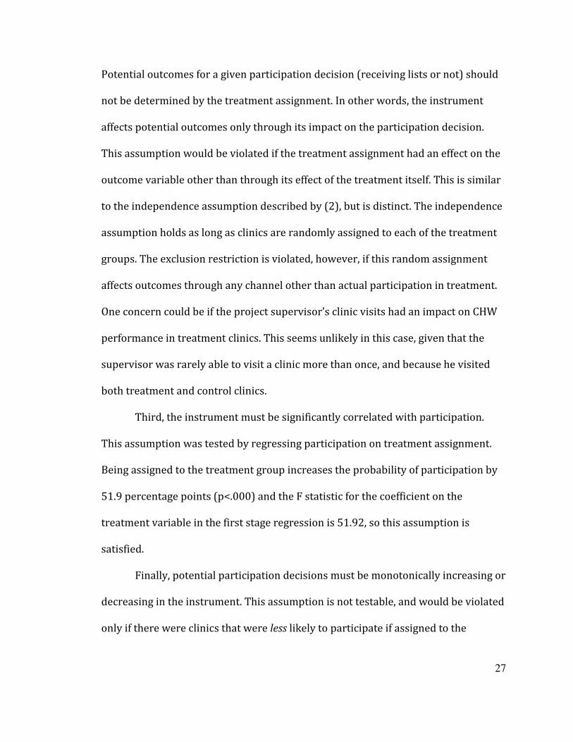
Potential outcomes for a given participation decision (receiving lists or not) should

not be determined by the treatment assignment. In other words, the instrument

affects potential outcomes only through its impact on the participation decision.

This assumption would be violated if the treatment assignment had an effect on the

outcome variable other than through its effect of the treatment itself. This is similar

to the independence assumption described by (2), but is distinct. The independence

assumption holds as long as clinics are randomly assigned to each of the treatment

groups. The exclusion restriction is violated, however, if this random assignment

affects outcomes through any channel other than actual participation in treatment.

One concern could be if the project supervisor’s clinic visits had an impact on CHW

performance in treatment clinics. This seems unlikely in this case, given that the

supervisor was rarely able to visit a clinic more than once, and because he visited

both treatment and control clinics.

Third, the instrument must be significantly correlated with participation.

This assumption was tested by regressing participation on treatment assignment.

Being assigned to the treatment group increases the probability of participation by

51.9 percentage points (p<.000) and the F statistic for the coefficient on the

treatment variable in the first stage regression is 51.92, so this assumption is

satisfied.

Finally, potential participation decisions must be monotonically increasing or

decreasing in the instrument. This assumption is not testable, and would be violated

only if there were clinics that were less likely to participate if assigned to the

28

treatment group, or more likely to participate if assigned to the control group. This

seems unlikely, so it is reasonable to assume that this is not the case.

If these four assumptions hold, then this instrument may be used to estimate

the average causal effect of the treatment on those induced to receive treatment due

to their treatment assignment (Imbens and Angrist, 1994; Angrist and Pischke,

2009). Thus, random assignment to treatment is valid as an instrument to identify

the treatment’s causal effect on children’s vaccination status if those children are

covered by PEC clinics with CHWs that received the lists because of the clinic’s

treatment assignment. Imbens and Angrist show that this LATE estimator is

equivalent to the ITT estimate divided by the difference in participation rates

between the two treatment groups, as follows:

(4)

The LATE is estimated in two ways. First, it is estimated using CHW

responses about whether they received the lists to indicate participation. The

second method codes all CHWs from the control group as non-participants. This is

because these CHWs provided implausible answers to other questions about the

lists: most said they had been receiving the lists for longer than the lists had actually

been distributed, and others said they had only received the lists in the last month.

The results of the second method are presented in column 3 of Table A.2.6 in the

Appendix.

E[Yic | Zc =1] − E[Yic | Zc = 0]E[Dc | Zc =1] − E[Dc | Zc = 0]

29

5. Results

5.1. Complete Vaccination

Table 2.7 presents the main results of this study. The main regression model

includes child’s baseline vaccination status (a dichotomous variable equal to one if

the child has all vaccinations recommended for his or her age at baseline), age and

its quadratic term, and strata dummies. The ITT estimates suggest that the offer of

treatment significantly increases children’s probability of having complete

vaccination for their age by 2.5 percentage points over the baseline rate of 67.2%

(column 1). The LATE estimate shows a stronger effect, increasing the probability

of complete vaccination by 4.7 percentage points (column 2). F-statistics for Chow

tests for significant differences in coefficients across subgroups are also reported.

When all control group clinics are coded as non-participants (D0c = 0), the LATE

estimate falls to 3.6 percentage points. This is explained by the fact that the

denominator of the Wald estimator is the difference in probabilities of treatment;

when the probability of treatment in the control group goes to zero, the

denominator increases, decreasing the overall estimate. These results are

presented in column 3 of Table A.2.6 in the Appendix.

As expected, the treatment effect varies significantly by child age, area, and

CHW characteristics. Examined by age, the treatment effect is small (0.016) and not

significant for children under 18 months. For children at least 18 months of age, the

effect increases in significance, though not in size, with the ITT and LATE estimates.

Looking just at children who are due for vaccines given at 18 or 48 months of age,

the vaccines with lowest coverage at baseline, the treatment increases complete

30

vaccination by 6.0 percentage points by the ITT estimate and by 11.9 percentage

points by the LATE estimate. This is consistent with the hypothesis that reminders

play a more important role for the later, more infrequent vaccines.

Isolating the population with the lowest rates of vaccination at baseline,

children due for vaccines at 48 months, the treatment effect reaches 4.7 percentage

points with the ITT estimates and 9.2 percentage points for the LATE estimate;

although these are significant at the ten percent level only, and these effects do not

vary significantly between children due for the 48-month vaccines and other

children.

Effects vary significantly by area of implementation, with a larger estimated

effect where CHWs were least likely to have received any lists at baseline (prior to

the intervention, some mobile medical teams provided lists of patients to target in a

sporadic, ad hoc manner). The effect is greatest in Chimaltenango, where 12% of

CHWs indicated that they had received lists with vaccination information in the last

month at baseline; children in the treatment group are 6.1 and 8.7 percentage points

more likely to have complete vaccination for their age by the ITT and LATE

estimates respectively. Effects in Sacatepéquez, where 71% of CHWs indicated that

they received lists with vaccination information at baseline, were lowest. This is also

the area where CHWs were least likely to use the new lists and were least

enthusiastic about the project, according to the project supervisor’s interviews with

CHWs.

Another factor influencing the treatment effect is how well CHWs are able to

understand and utilize the PTLs. Where CHWs have at least completed primary

31

school (6 years of education), the treatment effect is greater, although it is not

significantly greater than the effect for CHWs who have not completed primary

school.

As expected, the LATE estimates of the treatment effect are higher than the

ITT estimates, significantly increasing the probability of complete vaccination by an

estimated 3.6-4.7 percentage points over the baseline rate of 67.2%. Tables A.2.6

and A.2.7 in the Appendix provide the results of further analysis of heterogeneous

effects by smaller age groups, and by baseline vaccination status. Effects are greatest

for older children and for children with incomplete vaccination at baseline.

5.2. Timely Vaccination

Even for those children who would have received all their recommended

vaccinations in the absence of the intervention, the intervention may have had an

effect on children’s likelihood of being vaccinated on time. On-time vaccination is an

important outcome, as timely vaccination reduces children’s exposure to vaccine-

preventable disease. It is also beneficial for children to receive their vaccines in a

timely manner because they are only eligible to receive PEC coverage until they

reach the age of five. Table 2.8 presents ITT and LATE estimates of the treatment

effect on the number of days after the child becomes eligible to receive a vaccine

that the child receives the vaccine, including only children who did receive the

vaccine. These estimates suggest that children in the treatment group who were

vaccinated have 3-7 fewer days of delay before receiving their vaccination by the

ITT estimates and 3-13 days fewer by the LATE estimates. These results should be

32

interpreted with caution, however, as they do not include children that have failed

to receive a vaccination. For this reason, if the intervention resulted in higher rates

of vaccination for children who were behind in vaccination, this could increase the

apparent delay in the treatment group, decreasing the estimated effect on days of

delay (making the program appear less effective).

To address this, Cox proportional hazard ratios, Kaplan-Meier survival

estimates and the results of log-rank tests of the equality of the survival functions

are presented. Table A.2.8 in the Appendix shows that the Kaplan-Meier survival

function for the treatment group lies almost entirely below the function for the

comparison group for the 18-month vaccines, and entirely below for the 48-month

vaccines. This means that for each number of days after a child becomes eligible for

a vaccine, a smaller percent of children in the treatment group remain unvaccinated.

The log rank test of difference in survival functions is not significant for the 18-

month vaccines, but is for the 48-month vaccines. This finding is consistent with

previous results showing that the treatment has a greater effect for children in these

age ranges.

To investigate this relationship further, a Cox proportional hazards model,

which allows for the introduction of covariates, was estimated for the 18-month and

48-month vaccines. These results are summarized in Table 2.9. According to these

estimates, the treatment does not have a significant effect on the hazard rate for the

18-month or 48-month vaccines.

5.3. Cost Analysis

33

Table 2.10 presents estimates of the cost of implementing patient tracking lists. The

actual cost of the inputs for this implementation are presented, including the

upfront fixed costs of purchasing one computer and printer per NGO. The variable

costs include toner, paper and hiring list facilitators for six months for each NGO.

The actual cost of implementing the intervention was $11,055. The average cost per

child in the treatment group was $1.65, or 21% of the total PEC budget per

beneficiary.

Table 2.10 also presents estimates of the cost of scaling up the intervention

to include control clinics in the four areas where the intervention took place. The

cost to scale-up the intervention is likely to be much lower than the cost to

implement the experimental intervention for several reasons. First, the list

facilitators, who were hired full time, indicate that it only took them one and a half

hours per month to generate all their monthly lists on average. If they were

generating lists for clinics in the control group as well, this could be expected to

increase to a total of three hours per month. The NGOs would be more likely to ask

existing staff to complete an additional task rather than hire an additional full time

staff person to complete a three-hour task. The cost for staff is then estimated at

NGO data entry staff’s monthly wage prorated to cover three hours of work per

month. The cost estimates for toner and paper are twice the actual cost since the

NGOs would produce lists for both treatment and control clinics. This is likely to be

a conservative estimate since the project provided the NGOs with a generous supply

of paper and toner. With these estimates, the cost of implementing the intervention

would be $0.17 per child for six months, or $0.34 for a year. This is equivalent to

34

4.25% of the PEC’s budget per beneficiary per year. Over the five years that a child is

covered by the PEC, this is $1.70. Based on the conservative ITT estimates of the

program’s effect on children’s likelihood of having complete vaccination, the

intervention would cost $6.85 per child with complete vaccination because of the

intervention. Using the LATE estimates, the cost is $3.64 per child with complete

vaccination because of the intervention. This estimate should be interpreted with

caution, however, as it is relevant for children at clinics induced to use the lists

because of their treatment assignment and does not include the null effect of the

intervention at clinics that choose not to use the lists. If this intervention were to be

scaled up or replicated in another area, the true cost would depend on the real take-

up of the intervention, which may not be complete. The results of the analysis by

subgroup indicate that PTLs are likely to be most cost effective in areas where

CHWs are currently not receiving lists at all.

6. Discussion

The estimates presented in this paper indicate that reminders to parents facilitated

by the distribution of PTLs increase children’s probability of receiving all

recommended vaccines for their age by 2.5 to 4.7 percentage points over a baseline

complete vaccination rate of 67.2%. The ITT estimates are policy-relevant, as they

capture the possibility that some clinics or health-workers would not use the PTLs;

these may be interpreted as a lower bound of the intervention’s effect, while the

LATE estimates may be interpreted as an upper bound, representing the

intervention’s potential in areas with higher take-up.

35

These results demonstrate that the distribution of PTLs to the CHWs

increased children’s probability of completing their recommended vaccines, but

they do not show how this happened. It is likely that the CHWs, armed with concise,

up-to-date information about which children need a vaccine that month, were more

able to target their reminders to the specific families that were due for a vaccine.

Since vaccination rates were higher at baseline for vaccines for children in their first

year of life, the effect of these reminders was expected to be lower in this group; the

results are consistent with this hypothesis. These reminders may have played an

important role for families of older children, however, who need vaccines less

frequently.

As their children grow older, parent perspectives on vaccination are likely to

change. Parents with older children have accumulated knowledge about vaccination

that parents of younger children have not. Their child may have had reactions to the

vaccine, such as fevers or aches (increasing the perceived cost of vaccination).

Furthermore, older children, who understand that a shot will hurt, may be more

likely to resist vaccination, further increasing the cost of taking the child for her

shots. Parents also may have observed that their child gets sick from time to time

despite having been vaccinated, which would decrease the perceived benefits of

vaccination. Additionally, parents may exhibit hyperbolic discounting, favoring

immediate benefits (not dealing with a screaming feverish child today) over

uncertain benefits in the future.

The results of the household survey are consistent with these learning

processes. Most parents agreed that their child was likely to have a reaction like

36

aches or a fever after receiving a vaccine: 80% of parents with babies under one

year agreed, and 92% of parents with children over one year did. This difference

shows that parents of older children are more likely to anticipate higher costs of

vaccination due to physical reactions. Parents of older children were also less likely

to agree that vaccines were important for preventing disease, and more likely to

agree that vaccines are more important for babies than for older children. Table 2.4

shows parent opinion on vaccination for families with younger and older children.

In addition to perceiving higher costs and lower benefits to vaccination,

vaccines for older children may also be harder to remember because they are given

less frequently. A personal reminder will help parents remember when their child is

due for a vaccine. It may also provide the encouragement necessary to overcome

parents’ inclination to put off today what can be done next month.

This intervention was inexpensive to implement within the PEC. Scaling up

the program is unlikely to require hiring additional personnel, as the data entry

personnel that are already in place could create the lists in a couple hours per

month. The greatest cost would be the recurring cost of paper and ink to print the

lists. As these NGOs operate on a very limited budget, this cost may be prohibitive.

From a social perspective, however, this investment is likely to be worthwhile for

the PEC.

Whether it would be worthwhile to create an electronic medical record

system in a country where such a system does not exist in order to implement an

intervention like this one would require an extensive cost-benefit analysis that is

beyond the scope of this paper. Ministries of health and non-governmental health

37

organizations around the developing world are increasingly dependent on

electronic medical records. Similar patient-tracking interventions may be beneficial

for these organizations.

7. Conclusion

This paper presents the results of a field experiment that introduced exogenous

variation in the likelihood that families receive personal reminders when their child

was due to receive a vaccine by distributing patient tracking lists to community

health workers responsible for outreach in their community. This intervention

increased a child’s probability of having completed all vaccinations recommended

for his or her age by 2.5-4.7 percentage points, over the baseline level of 67.2%. For

children due for vaccines at 48 months of age, the vaccines with the lowest rate of

coverage, this intervention increases their likelihood of receiving all recommended

vaccines by 4.7-9.2 percentage points over a baseline rate of 35%. Reminders do not

directly alter the benefits or costs of vaccination; however, these reminders increase

parents’ likelihood of following through with vaccinating their child, particularly for

older children. Nearly all parents in this sample indicate that they believe that

vaccines improve child health and plan to complete all recommended vaccines for

their children. This is a low cost intervention if electronic vaccine data and

community health workers are already in place. In similar situations, this is a cost-

effective intervention that may be important in improving vaccination rates and,

thereby, reducing child mortality among populations that remain unvaccinated.

38

Table 2.1: Health and Well-being in Guatemala

Indicator National Rural Urban Study samplee

Children’s healtha Infant mortalityf 34 38 27 18.7 Child mortalityg 42 48 31 30.7 Chronic malnutrition (ages 3-59 months)h 43.4% 51.8% 28.8% 45.1% Chronic malnutrition (ages 3-23 months)h 38.4% . . . Children with no vaccine, 12-23 months 1.7% 1.7% 1.8% 0.6% Children with all vaccines, 12-23 monthsi 71.2% 74.6% 65.5% 63.6% Women’s healtha Fertility ratej 3.6 4.2 2.9 3.5 Use of modern family planning methods 44.0% 36.2% 54.6% 41.8% Socioeconomic indicators Povertyb 51.0% 70.5% 30.0% 52.1% Extreme povertyb 15.2% 24.4% 5.3% 15.5% Net enrollment – primary schoolc 95.8% . . 90.7% Net enrollment – lower secondary schoolc 42.9% . . 42.0% Literacyc 81.6% . . .

a Encuesta Nacional de Salud Materno Infantil (ENSMI) 2008/2009, Ministerio de Salud Pública y Asistencia Social. b Encuesta de Condiciones de Vida (ENCOVI) 2006. Instituto Nacional de Estadísticas. c Resultados departamentales de la Encuesta de Condiciones de Vida 2006 (ENCOVI). Instituto Nacional de Estadísticas. http://www.ine.gob.gt/np/encovi/encovi2006.htm d Anuario Estadístico 2010, Ministrio de Educación. http://www.mineduc.gob.gt/estadistica/2010/main.html e Weighted average of department-level indicators for the departments of Sacatepéquez, Izabal (department of El Estor and Morales) and Chimaltenango. Weights are 2009 department level population projection. f Infant mortality is the number of deaths before age 1 per 1,000 live births. g Child mortality is the number of deaths before age 5 per 1,000 live births. h Children are considered to be chronically malnourished if their height for age is more than two standard deviations below the mean for their age. Data for 3-23 months age group only available at national level. i These include vaccinations against tuberculosis; the diphtheria, pertussis and tetanus shot at 2, 4 and 6 months; the polio shot at 2, 4 and 6 months; and measles. j This is the total fertility rate, which may be interpreted as the average number of children a woman would have in her entire life, averaging rates for all age groups.

39

Table 2.2: Coverage, Delay by Vaccine

Vaccine Age Coverage: Guatemala

Coverage: Study sample

(Baseline)

Days delay: Study sample

(Baseline) Tuberculosis Birth 96% 97% 44.2 Pentavalentd 1 2 months 97% 96% 37.3 Polio 1 2 months 96% 97% 37.3 Pentavalent 2 4 months 94% 94% 57.2 Polio 2 4 months 92% 95% 57.2 Pentavalent 3 6 months 86% 93% 76.1 Polio 3 6 months 86% 93% 76.5 MMRe 1 year 88% 90% 38.0 DTPf booster 1 18 months 82%c 76% 61.6 Polio booster 1 18 months 82%c 76% 61.2 DTP booster 2 48 months 33%c 35% 13.0 Polio booster 2 48 months 33%c 35% 7.1 Complete vaccination All ages . 67% .

a Following the ENSMI, for vaccines given at birth through 12 months, coverage is percent of children aged 12-59 months with the vaccine. For vaccines given at 18 months and 4 years, coverage is percent of children under five with the minimum age for the vaccine with the vaccine. b Encuesta Nacional de Salud Materno-Infantil (ENSMI). 2009. c Data from the National Immunization Program d Pentavalent: Pertussis, tetanus, diphtheria, hepatitis B, and influenza B. e MMR: Measles, mumps and rubella. f DTP: Diphtheria, tetanus, and pertussis.

40

Table 2.3: Access to PEC Services n Mean

Getting to the clinic Average distance traveled to clinic (km) 1,242 0.67 Average minutes to clinic (minutes) 1,246 15.25 Had to pay to get there 1,249 0.02 Had trouble getting to the clinic 1,249 0.02 Waiting times Received attention within half an hour 1,249 0.49 Received attention within an hour 1,249 0.83 Received attention in more than an hour 1,249 0.17 Went, but did not receive attention 1,249 0.00 Care Providers Doctor 1,236 0.48 Nurse 1,236 0.62 CHW 1,236 0.31 Services Received Last Visit Measured child height 1,176 0.42 Weighed child 1,176 0.91 Vaccinated child 1,176 0.50 Provided information on benefits of vaccination 1,176 0.45 Informed parent when child was due for vaccine 1,176 0.44 Recommended vaccination 1,176 0.43 Blood test 1,176 0.02 Gave medicine 1,176 0.47 Gave vitamins 1,176 0.66 None of the above services 1,176 0.00 Source, Cost of Curative Care When Sought Went to PEC clinic last time child was sick 1,274 0.57 Had to pay (those that went to PEC clinic) 724 0.02 Had to pay (went to other clinic) 457 0.33

Source: Household survey data

41

Table 2.4: Parent Perspectives on Vaccination

Families with only

babies under 1 year

Families with

children over 1 year

Percent

agree Percent

agree Diff.

Costs "I have had bad experiences with vaccines in the past" 19.0% 19.6% 0.6% "If my child receives a vaccine, he/she is likely to have a reaction like aches or a fever" 80.2% 91.5% 11.3%*** Benefits "Vaccines are effective in preventing disease" 100.0% 97.7% -2.3%* "Vaccines are more important for babies than for older children" 71.1% 76.0% 4.9% "I believe vaccines improve children's health" 100.0% 99.2% -0.8% Perspective "I believe my children will receive all recommended vaccines" 98.4% 97.4% -1.0% "It is difficult for parents like me to obtain all the recommended vaccines for their children" 40.5% 37.1% -3.4% "Most of my friends' children receive all recommended vaccines" 76.9% 79.0% 2.1% Number of observations 121 1190 1311

* p < .10; ** p < .05; *** p < .01.

Table 2.5: Sample

Area

Number of clinicsa

with EMR data

Number of Community

Health Workers

Households in household survey data

Children under 5 in EMR data

% treated children

Chimaltenango 32 43 314 2,773 53% Izabal - El Estor 45 48 345 3,787 57% Izabal – Morales 35 46 231 3,311 49%

Sacatepequez 18 44 420 3,085 47% Total 130 181 1,310 12,956 52%

a This table represents the sample used for analysis and excludes clinics for which endline CHW survey data are not available.

42

Table 2.6: Data management by treatment group from endline survey

Variable n Mean -

Control Mean -

Treatment Diff. p-value

CHW endline survey responses Received new lists - All 181 0.141 0.635 0.500*** 0.000

Chimaltenango 43 0.100 0.652 0.555*** 0.000 El Estor 48 0.208 0.625 0.397*** 0.004 Morales 46 0.136 0.875 0.730*** 0.000 Sacatepéquez 44 0.105 0.400 0.303** 0.039

Keeps own record of patient services 181 0.929 0.979 0.039 0.192 Knows who needs services next month 181 0.976 1.000 0.022 0.122

Planned who to remind with a list 181 0.412 0.583 0.194*** 0.006 Reminded people of visit 181 0.988 0.990 0.001 0.962 Reminded specific people of visit 181 0.871 0.958 0.082** 0.039 Received lists from mobile medical team, including: 181 0.659 0.792 0.137** 0.037

Vaccination information 181 0.576 0.792 0.215*** 0.002 Children to weigh 181 0.565 0.604 0.052 0.453 Children needing micronutrients 181 0.282 0.469 0.186*** 0.005 Children needing deworming 181 0.365 0.583 0.227*** 0.001 Prenatal checks 181 0.353 0.385 0.034 0.627 Family planning 181 0.212 0.281 0.073 0.227 Women needing micronutrients 181 0.235 0.323 0.079 0.213 Women needing vaccines 181 0.294 0.385 0.089 0.210 Post-natal care checks 181 0.165 0.250 0.089 0.115

Hours spent maintaining own record 177 8.410 10.415 1.731 0.527 Own record included vaccine information 181 0.718 0.771 0.051 0.386

Household observations Percent families ever visited by CHW 1,190 0.820 0.779 -0.041 0.083 Percent families visited by CHW in last month 919 0.777 0.804 0.027 0.331

Respondent has seen CHW’s patient lists 950 0.160 0.207 0.047 0.068

Strata dummies are included in regressions; standard errors are clustered at the clinic level. * p < 0.1; ** p < 0.5; *** p < 0.01.

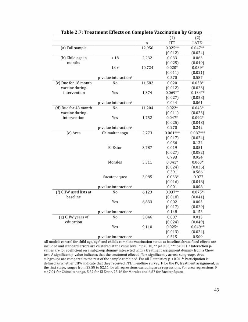
43

Table 2.7: Treatment Effects on Complete Vaccination by Group (1) (2) n ITT LATEb

(a) Full sample 12,956 0.025** 0.047** (0.012) (0.024)

(b) Child age in < 18 2,232 0.033 0.063 months (0.025) (0.049)

18 + 10,724 0.020* 0.039* (0.011) (0.021) p-value interactiona 0.570 0.587

(c) Due for 18 month No 11,582 0.020 0.038* vaccine during (0.012) (0.023) intervention Yes 1,374 0.069** 0.134**

(0.027) (0.058) p-value interactiona 0.044 0.061

(d) Due for 48 month No 11,204 0.022* 0.043* vaccine during (0.011) (0.023)

intervention Yes 1,752 0.047* 0.092* (0.025) (0.048) p-value interactiona 0.270 0.242

(e) Area Chimaltenango 2,773 0.061*** 0.087*** (0.017) (0.024) 0.036 0.122 El Estor 3,787 0.019 0.051 (0.027) (0.082) 0.793 0.954 Morales 3,311 0.041* 0.063* (0.024) (0.036) 0.391 0.586 Sacatepequez 3,085 -0.033* -0.077 (0.016) (0.048) p-value interactiona 0.001 0.008

(f) CHW used lists at No 6,123 0.037** 0.075* baseline (0.018) (0.041)

Yes 6,833 0.002 0.003 (0.017) (0.029) p-value interactiona 0.148 0.153

(g) CHW years of No 3,846 0.007 0.013 education (0.024) (0.049)

Yes 9,110 0.025* 0.049** (0.013) (0.024) p-value interactiona 0.515 0.509

All models control for child age, age2 and child’s complete vaccination status at baseline. Strata fixed effects are included and standard errors are clustered at the clinic level. * p<0.10, ** p< 0.05, *** p<0.01. a Interaction p-values are for coefficient on a subgroup dummy interacted with a treatment assignment dummy from a Chow test. A significant p-value indicates that the treatment effect differs significantly across subgroups. Area subgroups are compared to the rest of the sample combined. For all F-statistics, p < 0.01. b Participation is defined as whether CHW indicate that they received PTL in endline survey. F for the IV, treatment assignment, in the first stage, ranges from 23.58 to 52.11 for all regressions excluding area regressions. For area regressions, F = 47.01 for Chimaltenango, 5.87 for El Estor, 25.46 for Morales and 6.87 for Sacatepéquez.

44

Table 2.8: ITT, LATE estimates of treatment on delayed vaccination (in days) Effect on vaccination Effect on delay

Min. age n ITT (SE)

LATE (SE) n ITT

(SE) LATE (SE)

Tuberculosis Birth 15,169 0.005 0.009 13,919 -3.098** -5.986** (0.005) (0.009) (1.308) (2.466) Pentavalent 1 2 mos. 14,891 -0.001 -0.002 13,405 -3.329** -6.445** (0.005) (0.009) (1.469) (2.913) Polio 1 2 mos. 14,891 -0.002 -0.004 13,414 -3.155** -6.116** (0.005) (0.009) (1.451) (2.912) Pentavalent 2 4 mos. 14,434 0.001 0.002 12,485 -3.552 -6.851 (0.006) (0.012) (2.198) (4.186) Polio 2 4 mos. 14,434 0.001 0.002 12,482 -3.785* -7.309* (0.006) (0.012) (2.156) (4.140) Pentavalent 3 6 mos. 13,890 -0.001 -0.002 11,692 -5.957** -11.533** (0.007) (0.014) (2.508) (4.919) Polio 3 6 mos. 13,890 -0.002 -0.003 11,708 -5.863** -11.364** (0.007) (0.014) (2.476) (4.869) MMR 12 mos. 12,491 0.005 0.010 10,484 -1.429 -2.761 (0.008) (0.015) (1.608) (3.123) DPT booster 1 18 mos. 10,724 0.007 0.013 7,479 -3.696 -7.190 (0.012) (0.023) (2.696) (5.072) Polio booster 1 18 mos. 10,724 0.003 0.006 7,495 -3.378 -6.574 (0.012) (0.023) (2.681) (5.079) DPT booster 2 48 mos. 2,973 0.017 0.033 1,135 -6.661** -13.119** (0.020) (0.038) (3.079) (6.221) Polio booster 2 48 mos. 2,973 0.020 0.037 1,138 -6.602** -13.027** (0.020) (0.038) (3.059) (6.113)

Strata fixed effects are included and standard errors are clustered at the clinic level. * p<0.10, ** p< 0.05, *** p<0.01. aDependent variable is a dummy variable indicating if the child has received each vaccine. The sample includes all children with at least the minimum age to receive each vaccine. Regressions were also run with a restricted sample of children who became eligible for each vaccine during the treatment period. Results were similar and are available upon request. bDependent variable is the number of days after the child becomes eligible to receive a vaccine that he or she receives the vaccine. The sample includes children who have received each vaccine.

45

Table 2.9: Survival Analysis for Vaccines at 18 and 48 months

Cox Hazard Ratios

Chi2 from Log-Rank test for Equality of Survival Functions

n (1) (2) (3) (4) Basic controls No No Yes No Strata Dummies No Yes Yes No DPT Booster 1 1,233 1.089 1.058 1.111 1.02 0.461 0.552 0.264 0.312 Polio Booster 1 1,231 1.051 1.028 1.080 0.36 0.518 0.456 0.231 0.548 DPT Booster 2 1,639 1.231 1.160 1.190 6.37** 0.162 .167 0.131 0.012 Polio Booster 2 1,831 1.215 1.151 1.177 5.62** 0.192 0.193 0.161 0.018

Standard errors are clustered at the clinic level. p-values are presented below hazard ratios (columns 1-3) and below chi2 (column 4). * p < 0.1; ** p < 0.05; *** p < 0.01 Basic controls include age, age2 and whether the child had complete vaccination at baseline.

46

Table 2.10: Cost Estimates

Budgetary Costs for

Study (six months)

Intervention's Economic

Costs

Estimated Economic Costs for Scale-up

(six months)

Estimated Budgetary Costs for Scale-up

(six months)

(1) (2) (3) (4)

Computers $3,421.05 $570.18 $570.18 $0.00 Printers $263.16 $43.86 $43.86 $0.00 Additional NGO Staff $6,315.79 $78.95 $157.89 $0.00 Toner $1,000.00 $1,000.00 $2,000.00 $2,000.00 Paper $55.26 $55.26 $110.53 $110.53 Total $11,055.26 $1,748.24 $2,882.46 $2,110.53 Children Under Five 6690 6690 12,956 12,956 Cost per Child Under Five $1.65 $0.26 $0.22 $0.16 Children with complete vaccination because of intervention (ITT)a 167 167 324 324 Cost per child with complete vaccination because of intervention (ITT) $66.10 $10.45 $8.90 $6.52 Children with complete vaccination because of intervention (LATE)b 314 314 609 609 Cost per child with complete vaccination because of intervention (LATE) $35.16 $5.56 $4.73 $3.47

(1) Budgetary costs include actual costs to implement the intervention for 6 months. (2) Economic costs include the cost of six months of computer use, estimated as one sixth of the total cost.

This uses straight-line depreciation assuming that the life of a computer is three years (see Wang et al., 2003). The staff costs are the cost of actual time spent working on producting PTLs, two hours a month, or 1/80 of one FTE.

(3) The economic costs for scale-up include the cost of six months of computer use using the same assumptions as in column (2). Staff, paper and toner costs are estimated as twice those in column (2) since list facilitators would produce lists for clinics in the control group as well as in the treatment group if scaled-up.

(4) Budgetary costs for scale-up include no additional costs for computers since the computers provided for the intervention could continue to be used. No staff costs are added since the NGOs could use existing staff to produce the lists.

a This is the number of children in the relevant sample multiplied by the ITT estimate of 2.4 percentage points. This number is doubled in columns (3) and (4) because children in the control group would benefit from the intervention under scale-up. b This is the number of children in the sample multiplied by the LATE estimate of 4.6 percentage points. This should be interpreted with caution, however, as this is the estimate for children at clinics that would receive the lists because of their assignment to treatment, without considering the null effect on children at clinics that do not use the lists when offered (see description of LATE estimates). This number is doubled in columns (3) and (4) because children in the control group would benefit from the intervention under scale-up.

47

Chapter 3:

Teacher Training and the Use of Technology in the Classroom:

Experimental Evidence from Primary Schools in Rural Peru

48

1. Introduction

The One Laptop Per Child (OLPC) Foundation’s computer, dubbed the “Green

Machine,” or the $100 laptop, made a splash when the OLPC Foundation’s founder,

Michael Negroponte, showcased it for the first time at a United Nations summit in

Tunis in 2005. Negroponte stated that his organization planned to sell millions of

the laptops for $100 each to developing country governments around the world

within a year. U.N. Secretary General Kofi Annan called the initiative “inspiring”

(BBC News, 2005). Governments would have to order a minimum of one million

laptops to participate.

The program has fallen short of initial high hopes that it would transform

learning in developing countries and close the digital divide in several ways. The

OLPC Foundation planned to require a minimum purchase of one million laptops,

but three years after the unveiling, fewer than one million laptops had been sold.

The “$100 laptop” has sold for $200 (The Economist, 2008). In 2012, researchers

published their findings that the laptops had no effect on math or reading skills

(Cristia et al., 2012; Sharma, 2012), and the Economist magazine wrote that by

buying the OLPC Foundation’s XO laptops, the Peruvian government, which has

purchased more laptops than any other country, had invested in “very expensive

notebooks” (The Economist, 2012).

While the scale of the OLPC program has fallen short of the Foundation’s

expectations, governments’ investments in the program’s laptops and other

computers for children cannot be called small. Peru’s government alone has spent

over $200 million to buy 800,000 XO laptops, and at least 30 other developing

49

country governments have invested in the $200 computers (The Economist, 2012).

This represents a major investment, especially when considering that low-income

countries spend $48 per pupil per year on education, and middle-income countries

spend $555 (Glewwe and Kremer, 2006).

In 2009, the Inter-American Development Bank (IDB) began a randomized

evaluation of the One Laptop Per Child Program in Peru, randomly assigning 210

schools to receive laptops and 110 schools to serve as controls. The authors found

that the program increases children’s abstract thinking, but has no effect on math or

language test scores (this is described in greater detail below) or motivation.

Policy-makers seeing the disappointing results of evaluations of the

expensive OLPC project are likely to wonder: Why do laptops fail to improve

children’s learning outcomes? What can be done to make them more effective? At

the end of the 2010 school year, the Ministry of Education in Peru’s General Office

for Education Technology (DIGETE) implemented a randomized experiment in

which teachers, students and parents at randomly selected schools that were

already using the laptops received training on how to incorporate the XO laptops

into the learning process and how to take care of them. This training program is

called the Pedagogical Support Pilot Program (PSPP). This chapter evaluates this

training’s impacts on how teachers and students use the laptops, on teacher and

student knowledge and opinions about them, and on student test scores.

The PSPP was an intensive teacher training program, which provided two

weeks of training to teachers in randomly selected schools over the course of one

month (in addition to the 40 hours of training that most teachers received upon

50

receipt of the laptops). The objectives of the PSPP included increasing teacher,

parent and student enthusiasm for the project; teaching teachers how to

incorporate the laptops into their curriculum; and teaching teachers, students and

parents how to take care of the laptops properly. This is discussed in greater detail

in Section 2.

This chapter evaluates the impact of this pilot by answering three questions.

First, did this training change teacher behavior? Specifically, did it increase

computer use, or change the type of applications that teachers and students use

most frequently? Secondly, can this type of teacher training improve student’s test

scores in math or verbal fluency? Thirdly, did this training affect teacher knowledge

or opinions of the XO laptops?

Data collected in 2012 for this research show that teacher and student use of

the XO laptops has declined since data were collected in 2010 for Cristia et al.’s 2012

evaluation. Although teachers dramatically increased their use of the laptops during

the training, teachers at schools that participated in the PSPP were no more likely to

use the laptops 18 months later. Surprisingly, teachers at treatment schools

reported using the computers less than teachers in control schools in the week prior

to the survey on average (p < 0.10). Teachers at schools that received the training

were no less likely to have trouble using the laptops, and they did not have more

positive opinions of the laptops.

The training did have an effect on what applications the teachers and

students used. Teachers at schools that received the training were more likely to use

applications that were covered in the training. Students in treatment schools used

51

music applications less frequently, and used math applications more frequently,

perhaps indicating more concentrated use of academic applications. There was no

effect on test scores. An objective assessment of how well the training carried out is

not available. A limitation of this essay is that without this information, it is not

possible to discard the possibility that the training’s lack of effect on many outcomes

was because the trainers did not carry out the training properly.

This chapter is organized as follows. Section 2 reviews literature related to

the use of technology in education. Section 3 provides background information on

education in Peru and the One Laptop Per Child program. Section 4 describes the

Pedagogical Support Pilot Program (PSPP) intervention and experimental design.

Section 5 presents the empirical specification. Section 6 presents results, Section 7

provides discussion of the results, and Section 8 concludes.

2. Literature Review

A large body of literature reviews the role of computers in education. The

evidence on computers’ impacts on learning is mixed, which is perhaps not

surprising, considering how dependent computers’ effects are likely to be on how

they are used (Penuel, 2006). Several papers have found that distributing

computers to students does not increase test scores. Angrist and Lavy (2002) use

instrumental variables to estimate the effect of the Tomorrow-98 program, in which

35,000 computers were distributed to schools across Israel. A town’s ranking for

eligibility in the program was used as an instrumental variable. The authors find

that the program had no positive effect on Hebrew test scores, and may have had a

52

negative effect on math scores. Leuven, Lindhal and Webbink (2004) use regression

discontinuity design (RDD) to estimate the effect of a program that subsidizes

purchasing computers and software for schools in which at least 70% of students

come from disadvantaged groups in the Netherlands. The authors find that this

program had negative effects on test scores. Malamud & Pop-Eleches (2011) also

use regression discontinuity design to evaluate the effects of a program that

subsidized the purchase of home computers in Romania for families with incomes

below an income cutoff. They find that home computer use led to declining test

scores in English, Romanian and math, but increased computer skills. Finally,

Barrera-Osorio and Linden (2009) implemented a randomized controlled trial and

found that even after providing teachers with months of training, a program that

distributed computers to schools in Colombia also had no effect on students’ time

spent studying or test scores, but did improve students’ computer skills.

Several studies have shown that interventions that incorporate software

with specific guidelines for how to use it can be effective. Roschelle et al. (2010)

evaluated one such program that provided hardware, software, worksheets, lesson

plans and in-depth teacher training, and found that it had significant positive effects

on test scores for students in the U.S. two RCTs. They found similar results when

estimating the effects for teachers in the control group that received the treatment

in the second year of the study. In another RCT, Banerjee et al. (2007) found that

students’ test scores increased by 0.47 standard deviations after using a math

program that was tailored to their ability for two hours a day in India. Rosas et al.

(2003) matched students in 30 classrooms by academic achievement and

53

socioeconomic characteristics to create a treatment group of classrooms, internal

control classrooms at the same schools, and external control classrooms at different

schools. They found positive effects of educational video games for students that

used the games for 30 minutes a day in Chile.

Several other studies suggest that successful interventions that use

computers may not necessarily be more effective than if a teacher delivers the same

material. Linden (2008) found that students in India benefited from using

educational software only when they used it in addition to class time, but not when

it displaced time in class. He, Linden and MacLeod (2007) found that students

benefited equally when the same material was delivered by computer as when it

was delivered by teachers with flashcards.

Researchers at the Inter-American Development Bank published the results

of the largest randomized controlled trial to evaluate the impact of “one-to-one”

computing, the distribution of one computer per child, in a developing country to

date (Cristia et al., 2012). The authors report that the One Laptop Per Child Program

dramatically increased students’ access to computers in participating schools in

Peru, but that the effects of this access were limited. The intervention had no effect

on enrollment or attendance, nor did it have an effect on how much time children

spent reading or doing homework. Students in the treatment group did not exhibit

increased motivation for school, while they demonstrated negative effects on their

self-perceived school competence. Most notably, the authors found no effect on

math or language test scores. The authors did find a significant positive effect on

students’ abstract reasoning. Hansen et al. (2012) also found that the XO laptops had

54

significant positive effects on children’s abstract reasoning in Ethiopia. This study

does not report effects on math or language test scores, but does report that there is

no effect on English, Math or overall grades.

In a review of the literature on one-to-one computing, or, the practice of

distributing one computer per student in schools, Penuel (2006) found that students

tend to use computers primarily for word processing, email or browsing the

Internet. They are less likely to use software programs that are specifically designed

to teach basic skills. Cristia et al. (2012) write that the OLPC program’s failure to

improve test scores in Peru may be explained by the “absence of a clear pedagogical

model that links software to be used with particular curriculum objectives.” This is

consistent with a qualitative evaluation of the program that found that the OLPC

program in Peru caused only modest, if any, changes in pedagogical practices

(Villarán, 2010). Cristia et al. write that this may be due to the absence of clear

instructions to teachers on how to use the laptops to achieve specific learning

objectives, and the lack of programs on the laptops that have a direct link to

curricular goals.

According to Cristia and colleagues’ evaluation, most students were using

their laptops; according to automatically generated logs on students’ laptops, 76.2%

of children used the laptop at least once in the last week. Simply using the

computers, however, did not appear to be enough for them to generate an impact on

learning. The program did not have an effect on intermediate variables that might

translate to higher test scores, like attendance, homework, or time spent reading.

55

Penuel (2006) reports that teachers use technology more often when they

perceive that its uses are closely aligned with their curriculum. Furthermore, when

teachers perceive the training activities to be relevant to their teaching, they are

more likely to integrate the technology into their teaching. In personal interviews

conducted for this research, teachers reported that they needed more training on

how to incorporate the laptops into their lesson planning. Severin & Capota (2011)

report that teachers in Uruguay expressed similar concerns about not knowing how

to use the XO laptops in their classrooms.

3. Background

3.1. Education in Peru

Education in Peru is compulsory and free of charge from preschool through

secondary school. As in many other Latin American countries, Peru has achieved

nearly universal access to primary education, with 98% of children between the

ages of six and 11 enrolled in primary school. Nonetheless, Peru still faces

challenges in improving the quality of education offered in its schools. The gross

enrollment rate of 108% reveals that overage children still crowd classrooms as

they work their way through primary school (UNICEF, 2013). While enrollment

rates are high, Peru’s primary school students lag behind the regional average in

reading and math test scores (PREAL, 2009). On Peru’s national tests, only 17% of

second graders were at grade level in reading, and just 7% were at grade level in

math (Cristia et al., 2012). Students in Peru’s rural areas lag behind students in

56

urban areas; in 2009, Peru’s urban-rural gap was greater than any other country’s in

a ranking of 16 Latin American countries (PREAL, 2009).

3.2. The One Laptop Per Child Program

A group from the Massachusetts Institute of Technology’s Media Lab established the

OLPC Foundation in 2005. After the Foundation’s program was unveiled at the

World Economic Forum in Davos, Switzerland, the United Nations Development

Program announced that it would work with the OLPC Foundation to support the

distribution of their laptops, known as the XO laptops, around the world (OLPC

Foundation, 2013a). Since then, the Foundation has distributed over 2.5 million

laptops to 42 countries around the world; more than 2 million of these were

distributed in Latin American countries (OLPC Foundation, 2013b). In most cases,

developing country ministries of education have purchased the laptops. Uruguay

was the first country to buy one laptop for every primary school child in 2008, while

Peru has bought more XO laptops than any country, with nearly 800,000 XO laptops

for students in 8,300 schools (Programa Una Laptop Por Niño Peru, 2013). This

represents approximately 20% of Peru’s primary school students.

The mission of the One Laptop Per Child (OLPC) Foundation is “to provide

children in developing countries with rugged, low-cost laptop computers that

facilitate collaborative, joyful and self-empowered learning”. This philosophy is

based on the Foundation’s five principles: child ownership (each child owns his or

her own laptop), low ages (the target population is primary school aged children

(ages 6-12), saturation (all children and teachers in a given community should have

57

a laptop), connection (laptops are designed to connect with nearby laptops without

relying on Internet), and open source (this should facilitate writing new applications

for the XO laptops) (OLPC Foundation, 2013c).

The XO laptop was designed for “exploring and expressing” rather than for

direct instruction (OLPC Foundation, 2013d). The laptop was designed to facilitate

sharing activities and collaborating with other children through a local wireless

network that does not rely on the Internet. A wide variety of applications are

available for the computers, which use a Linux-based operating system, compatible

with open-source software. When the program launched in Peru, the Ministry of

Education selected 39 applications to load onto the laptops in Peru from a wide

variety of applications. These applications can be classified into five groups:

standard (Write, Browser, Paint, Calculator and Chat), games (Memory, Tetris,

Sudoku, Maze and others), music (TamTam Edit and others to create, edit and play

music), programming (three programming environments are available) and others

(Wikipedia with hundreds of entries available offline, sound and video editing). The

laptops also come loaded with 200 children’s e-books (Cristia et al., 2012).

3.3. The One Laptop Per Child Program in Peru

The OLPC program began in Peru in 2009. The Ministry of Education introduced it

first in the country’s multigrade schools – small, rural schools in which teachers

teach multiple grades in the same classroom. The program was seen as a way to

address the urban-rural achievement gap and to bridge the digital divide. The stated

objectives of the program were:

58

1. To improve the quality of public primary education, especially that of children in the remotest places in extreme poverty, prioritizing multi-grade schools with only one teacher.

2. To promote the development of abilities recommended by the national curriculum through the integration of the XO computer in pedagogical practices.

3. To train teachers in the pedagogical use (appropriation, curricular integration, methodological strategies and production of educational materials) of portable computers to improve the quality of teaching and learning (Program Una Laptop Por Niño Perú, 2013).

According to Oscar Becerra, who led the introduction of the program in Peru,

the program was also seen as a strategy to overcome the challenge of having poorly

prepared teachers (Becerra, 2012b). A 2007 census of 180,000 teachers in Peru

revealed that 62% of teachers did not reach reading comprehension levels

“compatible with elementary school (PISA level 3)”, while 27% of them scored level

0. In math, 92% failed to reach 6th grade level performance in math (Becerra,

2012a). The hundreds of e-books and Wikipedia entries available on the laptops

might give children in schools with no or poorly equipped libraries access to

literature that they otherwise would not have. Furthermore, the software, designed

to facilitate child-led activities, might provide children with additional stimulation.

4. Teacher Training Intervention & Experimental Design

Teachers at all schools receiving the XO laptops are expected to attend a 40-hour

training aimed at informing teachers on the mechanics of how to use the laptops and

their software. In survey data collected in 2010 for Cristia et al.’s 2012 paper, 67%

of teachers that were participating in the OLPC project reported that they had

59

received training on how to use the laptop. Of those, 68% indicated that they had

received five days of training, as MINEDU had planned. 23% received fewer than

five days, while 9% received more. During the first year of OLPC implementation,

teachers expressed interest in receiving further training on how to use the laptops,

stating that the initial training was not enough for them to understand how to

incorporate the laptops into their curriculum (personal interviews, 2012; DIGETE,

2010). In personal interviews conducted at the end of 2012 for this essay, several

teachers mentioned that they felt “abandoned” and left to learn how to incorporate

the laptops into their lessons on their own after the initial training. This problem is

aggravated by high rates of teacher turnover, as teachers who are new to schools

with XOs lack even the initial training. For example, 28% of the teachers surveyed

for this research in 2012 were new that year. This is driven by teachers changing

schools; only 8% of those new teachers were first year teachers.

In 2010, short-term results from the IDB’s evaluation of OLPC were

presented to the government, showing that although students used the laptops

frequently, the program had no effect on learning outcomes, and students in schools

that received the laptops displayed decreased motivation for school. In response to

these findings and to teachers’ requests for additional training, authorities at the

Ministry of Education’s Office for Educational Technology (DIGETE) developed the

Pedagogical Support Pilot Program (PSPP).

60

4.1. The Intervention: The Pedagogical Support Pilot Program

The DIGETE describes the PSPP as a “planned, active and participatory orientation,

focused on strengthening teachers’ abilities to use and integrate the XO laptops into

the teaching and learning process.” The program has two objectives, which are

summarized in Table 3.1. The first objective is to increase teachers’ use of the

laptops as a part of the teaching and learning process; this is defined as using the

laptop as a tool for a student to reach some learning goal. The second objective is to

increase awareness among students and parents of the laptops’ potential as an

educational tool (DIGETE 2010a). Teachers, students and parents all participated in

the PSPP.

The training took place over the course of four weeks in each school between

October and December, at the end of the 2010 school year. The trainer spent the

entire first week at the school, left for two weeks, then returned in the fourth week.

The program consisted of three components: observation, awareness raising, and

reinforcement. The trainers included technology specialists from the Office for

Education Technology (DIGETE) at the Ministry of Education, university and

community college teaching students, and OLPC Foundation volunteers. All trainers

underwent a detailed training. DIGETE published a detailed report on the training,

which describes which specific components were carried out and in which schools

(DIGETE, 2010b).

Regional authorities from the Ministry of Education supervised the trainers

in the field. They held weekly meetings, and maintained regular communication

with the trainers by phone between meetings. Finally, they reviewed the data the

61

trainers collected during the training. Working with the trainers and officials from

the central Ministry of Education office, these regional authorities wrote a final

report (DIGETE, 2010b). According to this detailed report, the trainers implemented

all components of the training as planned in all schools.

4.1.1. Observation

To fulfill the observation component, at the beginning of the first and second weeks

at the school, the trainers reviewed the teacher’s lesson plans (if he or she had any),

observed the lesson, and reviewed the log files on two students’ laptops. The

observation served to orient the trainer to the teachers’ current level of knowledge

about the laptops and how he or she was incorporating them into the lessons, as

well as to collect data on how teachers and students used the laptop at the

beginning of the first and second weeks of training.

4.1.2. Awareness-raising

The objective of the awareness-raising portion of the training was to convey the

importance of the laptops as a learning tool to teachers, families and students. For

teachers, this also included training on how to use specific applications and how to

incorporate them into their lesson planning. At each school, the trainers began with

a group training for all the teachers, and followed the group training with

demonstration lessons in each teacher’s classroom. At the group training, the trainer

explained how the program could benefit teachers and students, what it means to

incorporate the laptop into the teaching and learning process, and discussed

62

challenges the teachers may face. The training emphasized the use of 10 priority

applications (Write, Paint, Speak, Record, Memorize, Scratch, EToys, Turtle Art,

TamTam Mini, and Browser) and five additional applications (Wikipedia, Chat,

Words, Measure and Puzzle). At the beginning of the training, the trainers observed

that most teachers only knew how to use the Write, Paint and Wikipedia

applications. During the demonstration lessons, the trainers provided specific

suggestions on which activities to use for various curricular areas and demonstrated

how.

Since one of the key objectives of the training is to motivate parents and

students to use the laptop, trainers held workshops with parents at every school.

The objective of this meeting was to provide parents and students with background

information on the OLPC program, to explain the importance of the laptops as a

learning tool, and to demonstrate how to care for the laptops. All parents were

invited, and 80% of parents attended the workshops (DIGETE, 2010b). The trainers

explained to the parents that they could support their children’s education by

encouraging them to use their laptop every day, both at school and at home. The

trainer spent time assuring parents that they would not have to pay if their child lost

or damaged their laptop. In some schools, parents agreed to make bags for the

children to carry their laptops back and forth between home and school (see Figure

3.1).

In workshops with students, the trainers encouraged the students to use

their laptop every day, both at school and at home, explaining that the laptop is a fun

way to learn about computers and other subjects. The trainers also demonstrated

63

how to keep the laptops clean and how to carry them between home and school

carefully.

4.1.3. Reinforcement

In the final phase of the training, the trainers conducted a series of interactive group

workshops with teachers (8-9 per school on average). In these workshops, the

trainers reviewed how to use the priority applications and how to integrate them

into lesson plans. They also covered basic troubleshooting techniques. These

workshops also provided a space for conversation and reflection. The Ministry’s

report on the training states that teachers, parents and students all displayed

increased enthusiasm for the laptops after the training.

4.2. Experimental Design

Schools were randomly selected to participate in the PSPP to facilitate its evaluation.

The study sample was comprised of the 52 schools from the treatment group of the

IDB’s ongoing impact evaluation of the OLPC program in the Junin department.

Junin was chosen because it is the department with the largest number of schools

from the IDB sample. Treatment was randomly assigned to half of these schools,

stratifying by 2009 school size and test scores. Each stratum included two schools

that were similar on enrollment and test scores. The random assignment generated

two groups that were balanced on most, but not all, characteristics (see Table 3.3).

The groups are balanced on school characteristics, including access to electricity

and Internet, and number of students. Teachers at the two groups of schools are

64

similar in terms of teaching experience and previous training with the XO laptops.

There are some differences, however. Teachers at treatment schools are

significantly less likely to have studied at a university rather than an instituto

(similar to a community college). In 2009, the school year prior to the training,

teachers in treatment schools were 20.9% more likely to have used a computer

before. Considering these two differences, it is unclear if one group would be better

positioned to benefit from the training than another.

Students in the two groups are similar in sex and age. Students in treatment

schools have 0.459 fewer siblings (which might be correlated with less

disadvantage), but travel 4.4 more minutes to get to school (which may be

correlated with more disadvantage). Although these differences are significant, they

are small in magnitude.

As described in Chapter 2, random assignment of treatment generates

treatment groups that are equivalent on observed and unobserved characteristics in

expectation. When a smaller number of units (or groups) is randomized, the

likelihood that the randomization will create equivalent groups declines. It is not

surprising that a larger number of significant differences were found in this

experiment in which 52 schools were randomized, as compared to the experiment

in Chapter 2 in which 167 clinics were randomized.

DIGETE, the Ministry of Education’s office for technology in education,

implemented the training along with the Educational Projects’ Pedagogical Area

office. According to their report on the training (DIGETE, 2012b), all schools in the

65

treatment group received the training, while no schools in the control group

received the training.

4.3. Data and Sample

The training was implemented at 26 schools that were randomly drawn from the 52

schools in the Junin department that are part of the IDB study. Junin is a department

just east of Lima with a diverse topography that includes mountains, high plains and

jungle areas. Spanish is the first language of 87% of Junin’s inhabitants, while

Quechua is the first language for 9% (INEI, 2007). As of 2004, over half of Junin’s

residents lived in poverty, while 20% of the population lived in extreme poverty

(World Bank, 2005).

The data for this chapter are a unique combination of survey data, test

scores, and log files from students’ computers. Table 3.2 summarizes the data

sources and sample sizes for each. Data were collected at all 26 control schools and

at 25 of the 26 treatment schools (because of time and budgetary constraints, it was

infeasible to visit one school, which would have required traveling one week to

reach) in mid-2012, two school years after the training, which occurred at the end of

2010. The principal surveys included basic school characteristics, such as the

number of students and teachers, access to infrastructure, and availability of the XO

laptops. Teacher surveys were longer, covering availability of laptops in their

classroom, use of the laptops by application and curricular area, knowledge of the

laptops and opinions of the laptops. Student surveys were short; students reported

whether or not they use an XO laptop at school or at home, and responded to

66

various questions about how they like to use the laptop. Data were also copied from

the log files of students’ laptops. This procedure was explained to students clearly,

who were given the option not to participate in the study (no students chose to opt

out).

Students took short tests in math and verbal fluency. Due to budgetary

constraints, they did not take the Raven’s tests used in the study by Cristia et al. To

test their abilities in math, the students were asked to complete as many of a long

series of addition problems of increasing difficulty as they could in two minutes.

Scores ranged from zero to 67, with an average score of 28.3. To measure verbal

fluency, students were given three minutes to write down every word they could

think of that began with the letter “t”. Scores ranged from 0 to 27 with an average

score of 8.5. Cristia et al. (2012) used the same test of verbal fluency and found that

the XO laptops had an effect equal to approximately six months of a child’s normal

progression, though this effect was not statistically significant.

Automatically generated log files were extracted from students’ laptops.

These log files are automatically generated and saved to the laptop, but only keep

information on the child’s last four sessions; records of all previous sessions are

automatically deleted. Children cannot modify the log files.

Up to 15 children were sampled at each school. To select the children,

enumerators randomly selected five children each from second, fourth and sixth

grades, for a potential sample of up to 15 children per school (the sample was

smaller whenever fewer than five children were enrolled in a grade). A total of 588

children took the tests and responded to the survey. This represents 22% of the

67

2,681 children enrolled at the 51 schools included in data collection, with an

average of 11.5 children surveyed per school. Some schools did not have five

children enrolled in grades two, four and six; for this reason, the sample is smaller

than would have been expected with fifteen children sampled per school.

All of the sampled children’s teachers and all school principals were

surveyed. This yielded a sample of 51 principals and 135 teachers (all but one of the

51 principals were also teachers). This represents fewer than three teachers per

school because all but three of the schools in the sample are multigrade, meaning

that teachers teach more than one grade. At many schools, teachers cover more than

two groups; 47% of schools in the sample have one or two teachers.

4.4. Compliance to Treatment

In this experiment, there was perfect compliance to treatment, in that all schools

that were assigned to the treatment group received the Pedagogical Support Pilot

Program (PSPP) training, while none of the schools assigned to the control group

received this training. The training was school-wide, including all teachers, and took

place over ten school days.

To confirm this, teachers were asked about the training they had received on

the XO laptops. Teachers were asked whether they had participated in group

training, typically delivered as a lecture with few interactive components, or if they

had received “accompaniment,” like the training offered through the PSPP. There

was no significant difference in group training, but teachers in treatment schools

were significantly more likely to report that they had received training with an

68

accompanier. In treatment schools, 43.3% of teachers report having participated in

training with an accompanier, but to 11.8% of teachers in control schools also did

(this difference is significant at the 1% level). Restricting the sample to teachers that

were working in the same school in 2010, the difference increases from 31.5 to 42.8

percentage points. Teachers in treatment schools also report having spent

significantly more days in training with an accompanier, and are significantly more

likely to report having had “hands-on follow-up training”. These results are

summarized in Table 3.4.

All teachers were expected to receive training when they first received the

laptop computers in 2009, which explains why teachers at control group schools

also report having received training, at least in part; the PSPP training was given

from October to December of 2010. While the distinction between capacitación

grupal (group training), which refers to a lecture-based training and training with

an acompañante, which is what the PSPP involved, is generally understood, some

teachers may have responded that they participated in a training with an

accompanier when the training they received was a traditional lecture-based

training. An additional possibility is that teachers may have received training after

the intervention, although this appears to have had affected a small number of

teachers; one teacher in the control group recalls participating in training with an

accompanier after 2010, while three teachers from the treatment group do.

69

5. Empirical specification

As was the case with the experiment in Guatemala presented in Chapter 2, the

random assignment to treatment at the school level generated exogenous variation

in the treatment, which permits the simple estimation of treatment effects as in

equation (1):

ys = α + β*Treatments + εs. (1)

where ys represents the outcome of interest for school s, Treatments represents the

treatment assignment of school s, and εs is the error term for school s. The only

school-level outcomes analyzed here are whether the principal indicates that the

school uses the XO laptops, and the school-wide ratio of functioning XO laptops to

student.

A modified version of equation (1) represents the equation used to estimate

the treatment effect on the teacher and child-level outcomes:

yis = α + β*Treatments + Xis’Γ + εis (2)

In equation (2), yis represents the outcome of interest for child or teacher i in school

s, Treatments represents the treatment assignment of school s, and εis is the error

term for child or teacher i in school s. For regression estimates with teacher-level

outcomes, the vector Xis includes teacher age (in years), sex, education level (coded

as a dummy for attaining college or university level education), years of experience

70

teaching primary school, grade level dummies and strata dummies. For student

regressions, this include age (in months), sex, number of siblings, number of

minutes to walk to school, grade dummies and strata dummies. In all regressions,

Huber-White robust standard errors, clustered at the school level, are used. Simple

estimates with no control variables are presented in the Appendix. Only post-

intervention data were collected for this research. As such, it will not be possible to

condition on pre-intervention characteristics, unless they are time-invariant.

In most cases, equations (1) and (2) are estimated using ordinary least

squares. For several outcomes, however, it is more appropriate to use models for

count data. This is necessary for variables that count the number of sessions a child

has or number of applications a child uses because the number of children that do

not use the XO laptops increases the frequency of zero values. For example, 67% of

children in the sample had no sessions on the XO laptop in the past week. Negative

binomial, Poisson and zero-inflated negative binomial models are used in these

cases. Several test statistics are available to determine which of these models is

most appropriate. The Poisson distribution has a sample mean equal to its sample

variance, whereas the sample variance of the negative binomial distribution exceeds

its sample mean. The zero-inflated negative binomial is used with distributions that

have “excess zeros”. Excess zeros are zeros that are generated by a different process

than generates the other values. In this case, a zero-inflated negative binomial is

appropriate when predicting the number of times an application is used, for

example, when some students are in classrooms with teachers that do not use the

laptops at all.

71

Because this analysis relies on data that were collected in 2012, and the

training took place at the end of 2010, these estimates reflect the effect of the

treatment after more than a year. At the time of the training, 35.6% of teachers in

the data for this study did not work at the same school in 2010, so they would not

have participated in the training. Any effect for these teachers would be a spillover

effect from working with teachers, principals and students that did participate in the

training. Children and families that participated in the training may also have

dropped out or changed schools, while all students who were in 5th or 6th grade

during the training would have graduated from primary school if they did not repeat

a grade. As with new teachers, effects for second graders, who would not have

participated in the training unless they repeated a grade, would be the effects of

attending a school where the training took place, and possibly having a teacher or

principal that participated.

The treatment effect is estimated in two ways for each outcome. The first

estimate is for the entire sample (of schools, teachers and children, depending on

the outcome), while the second uses the sample of teachers who were at the same

school in 2010 and their students. Estimates based on the sample that is restricted

to teachers who were at the same school in 2010 will still be unbiased since they

compare teachers that have been at the same school for two years in both the

treatment and control groups. Estimates based on the restricted sample represent

the direct effect of participating in the training after two school years, while

estimates based on the entire sample represent the average effect for the school,

including any dilution of the effect due to teacher and student turnover.

72

6. Results

6.1. Immediate Effects

As was described in Section 4, the trainers collected data on how teachers

incorporated the use of the XO laptops into their lesson plans and their lessons

during the first week of the training, and during the follow-up week, three weeks

after the first week. Because these data were collected as part of the training, these

are not available for control schools. Table 3.5 summarizes data collected by the

trainers before the training and in the last week of the training. These immediate

effects of the training showed that teachers began using the laptops more

frequently, and with a wider variety of applications by the trainers’ second visit.

These changes in behavior exhibited by teachers between the first and last weeks of

training are likely to differ from changes in behavior that teachers would have

exhibited if the training had ended after the first week since some teachers may

have increased their use of the XO laptops in an effort to please the trainers. With

this in mind, these changes demonstrate that teachers became aware of additional

applications and learned some ways to incorporate them into their lessons.

Whereas in the first visit, only 64% of teachers could execute basic tasks on

the XO like saving files to a USB or sharing files with other computers, at the

beginning of the second visit, 95% or more of the teachers could do these things.

The percent of teachers that included the XO laptops explicitly in their lesson plans

increased from 13% to 73%, and the average number of activities they planned with

the XOs increased from 1.15 activities over the last three lessons in seven curricular

73

areas to 11.18 activities. This demonstrates that the teachers acquired basic skills

with the laptops and that they had the ability to incorporate the laptops into their

lesson plans.

The rest of the analysis focuses on whether participating in the training had a

lasting effect from the end of 2010 to early 2012 on use of the laptops and on

teacher and student opinions of the laptops.

6.2. Main effects

The PSPP had few significant effects on barriers to use, computer knowledge and

opinions, or use of the XO laptops according to surveys and computer logs; this is

likely to be driven at least in part by low statistical power. For the estimates

discussed in this section, the treatment effect is estimated in two ways for most

outcomes: first, for the full sample, and second, for the sample of teachers who

worked in the same school at the time of the training in 2010. Effects on school-level

outcomes are only estimated for the full sample.

6.2.1. Barriers to Use

One of the objectives of the training was to educate teachers on how to use, care for

and troubleshoot the laptops, which may have translated into increased numbers of

functioning laptops available for use. Teachers, parents and students were all taught

how to keep the laptops clean and carry them between school and home carefully.

The training included the steps necessary for teachers to activate the laptops, an

administrative hurdle that sometimes keeps teachers from using the laptops.

74

Finally, if the training succeeded in the objective of increasing enthusiasm for the

laptops, this may have increased teachers’ and students’ interest in taking care of

the laptops. With increased information on and interest in caring for the laptops, the

teachers may have been able to keep laptops from being lost or broken. However,

there is no significant effect on the number of laptops available per student or on

whether a teacher uses laptops; in fact, the coefficient estimates suggest that the

training was negatively associated with continuing to use the laptops (reported in

Table 3.9).

Table 3.6 reports the treatment effect on the likelihood that teachers report

facing various barriers to using the XO laptops: problems with electricity access,

with activating the laptops, with laptops breaking, connecting to the local network

known as the “neighborhood”, understanding applications, using the touchpad or

mouse or an index of all six potential problems. The training did not significantly

reduce teacher-reported trouble with any of these in the full sample or the 2010

teacher sample, although the effect is negative (indicating fewer problems) for five

out of the six outcomes. Surprisingly, the treatment effect on the having trouble

using the neighborhood network is positive and significant, indicating that teachers

in the treatment group were 20.5 percentage points more likely to have trouble

connecting to the local network, or to have never tried connecting. It could be that

teachers in the treatment group are more likely to have had more experience with

the local network, giving them more opportunities to have had trouble with it.

75

6.2.2. Teacher PC Use, XO Knowledge and Opinions

The schools in the study are in rural areas where, prior to the OLPC program, many

teachers had not used a computer before. During the first week of the training,

nearly one in four teachers did not know how to use a mouse. Table 3.7 presents

estimates of the training’s effect on teachers’ personal computer use and knowledge,

and knowledge of the XO laptops. The training significantly increased teachers’

likelihood of having used a PC in the last week, increasing the likelihood by 15.3

percentage points (p < 0.05). There was no effect on Internet use, or on teachers’

self-reported computer skills. More surprisingly, there was no significant effect on

teachers’ knowledge of the XO laptops, and five out of six coefficient estimates were

negative for teacher knowledge of using the Calculate application and accessing

texts.

In the teacher survey, teachers were asked whether they agreed or disagreed

with a series of statements about the XO laptops, such as, “The laptops are just for

playing,” or “Children learn more working on a laptop than on paper.” The estimated

effect of the training was negative for both estimates; for the 2010 teacher sample,

the training significantly decreased teachers’ score on an eight-point index of

positive opinions about the XO laptops by 0.824 points (p < 0.01), suggesting that

the training was not successful in one of its main objectives to increase enthusiasm

for the laptops.

76

6.2.3. Student PC Use and Opinions

Table 3.8 presents effects on student personal computer use at home and student

opinions of the XO laptops. The training did not have a significant effect on the

overall likelihood that students’ families would own a computer, but it did

significantly increase fourth graders’ families’ odds of owning a personal computer

by 9.4 percentage points in the full fourth grade sample and by 10.1 percentage

points in the sample of fourth graders whose teachers were at the same school in

2010 (p < 0.01 for both estimates). The fourth graders would have been in second

grade at the time of the training. The coefficients were positive, though not

significant for second graders, but negative for sixth-graders (and not significant).

Teachers’ and families’ increased PC ownership suggest that the training may have

been successful in increasing enthusiasm for computers among families of younger

students, but not older students.

In the student survey, students expressed their preferences for working on a

laptop over various alternatives for learning and for play. The training did not have

a significant effect on an index of positive opinions about the laptops, but the

coefficient estimates are negative overall and for each grade in both samples. The

coefficient estimates suggest that older children may have more negative opinions

about the laptops. A potential explanation is that the novelty may wear off for

students who have used the laptops for a number of years.

77

6.2.4. Laptop Use According to Survey Data

Table 3.9 presents effects on XO use according to principal and teacher survey data.

These results suggest that the strong effects the training appeared to have on the

variety of applications teachers used and the frequency with which they used them

during the training faded after two years. The training did not have a significant

effect on the likelihood that a school or classroom abandoned the program

altogether; in fact the point estimates are negative. The training did not have an

effect on teacher-reported use for any of the curricular areas. Although the training

provided the teachers with training on 15 specific applications, the estimated effect

of the treatment on the number of different applications used was -0.217 for the full

sample and -0.305 for the 2010 teacher sample (significant at the 10% level for the

2010 sample). The training also had a significant negative effect on the intensity of

XO use, defined as the number of applications used multiplied by the number of

times they use them, reducing the number of reported application uses in the last

week by 0.349 uses in the full sample (p < 0.1) and by 0.458 uses in the 2010

teacher sample (significant at the 5% level).

Panel B of Table 3.9 shows that although the training did not increase

teacher-reported use of the laptops, it did appear to have a significant effect on

which programs they used. Of the applications that they reported using, the

applications that were covered in the training represented a significantly greater

proportion of the applications that teachers used.

Student survey data provided further evidence that the training did not

increase use of the laptops. Panel C of Table 3.9 suggests that the training also failed

78

to have a significant lasting effect on another goal: encouraging students to bring

their laptops home. There was no significant effect on children’s likelihood of

bringing the laptop home. Surprisingly, despite the trainers’ efforts to alleviate

parents’ concerns about bringing the laptops home, students at treatment schools

were no more likely to bring their laptops home, and were somewhat less likely to

report having teacher or parent permission to bring their laptop home.

6.2.5. Laptop Use According to Logs

The laptops’ logs provide an objective source of data on how students use their

laptops, capturing data on the most recent four sessions on the laptop. Looking at

activity in the most recent week, 35% of children in the control group used their XO

in the past week, compared to 31% of children in the treatment group (see Figure

3.2 for more detail). The results presented in Table 3.10 show that the treatment

had a negative effect on the average number of sessions in the last week. The

treatment effect was significant and negative for the 2010 teacher group, reducing

the number of sessions by 0.390 sessions (p < 0.05). Looking at the treatment effect

by grade, the effect is significant and negative for 4th graders and 6th graders in the

2010 teacher sample.

Table 3.11 presents information from the logs on the types of applications

students use. In contrast to estimates based on teacher-reported use data, there is

no evidence in the logs that the training increased the use of the applications

covered in the training as a percentage of all application uses, although it did

significantly increase the use of math applications and programming applications in

79

the 2010 teacher sample and decrease the use of music applications. This could be

interpreted as teachers using the computers for more academic pursuits.

6.2.6. Child test scores

Table 3.12 shows that the training had no significant effect on children’s test scores

in math or verbal fluency. This is not a surprising result, given that the training did

not have large effects on frequency of laptop use, had few significant effects on the

type of use, and that overall levels of use appear low.

While none of the coefficient estimates are significant, the results suggest

that the training was more useful for fourth and sixth graders than for second

graders. Both coefficient estimates are negative for second graders’ verbal fluency

and math scores. For math, the treatment effect is -0.258 standard deviations for the

overall sample and -0.287 for students whose teachers were at the same school in

2010. In contrast, effects for fourth and sixth graders range from 0.210 to 0.256. The

treatment effect for second graders’ verbal scores was -0.097 for the full sample and

-0.062 for students with teachers that were at the same school in 2010. For fourth

graders, the effects are 0.221 and 0.261 for these same groups, respectively. For

sixth graders, the effects fall to 0.160 and 0.151. The effect for the combined sample

of 4th and 6th graders is still not significant at the 10% level, although p < 0.15 for

math scores.

80

6.2.7. Subgroup Effects

Treatment effects were also examined by subgroups: teacher age (above age 40 or

not; Table 3.13), teacher education (college or university degree or not; Table 3.14),

student gender (Table 3.15), and student grade (Table 3.16). This analysis was only

done for several key outcomes. For teacher regressions, these include the indices of

positive opinions and trouble with the laptops, whether the teacher reports using

the laptops at all, and the number of reported uses in the last week. For student

regressions, these include the index of positive opinions, test scores, and the

number of sessions in the last week.

The training’s negative effect on teachers’ opinions of the laptops is driven by

younger teachers and less educated teachers. Meanwhile, younger teachers and

more educated teachers drive the negative effect on teachers’ likelihood of using the

laptops at all. The training reduced the intensity of use more for older teachers than

for younger teachers. These diverse effects do not reveal that the training had

positive effects on opinions or use for some group; rather, it appears that the small,

negative effects were generalized by teacher age and education level.

There were no significant effects for the entire sample, or for any of the

subgroups examined at the student level. The training did not have significant

effects on student opinions, test scores, or laptop use for the full sample, for boys or

girls, or for any specific grade.

81

7. Discussion

Research by Cristia et al. (2012) has established that the OLPC program has not had

a significant effect on children’s learning as measured by reading and math scores.

Can anything be done to salvage Peru’s $200 million investment? The results

presented in the previous section show that providing intensive teacher training on

how to incorporate the laptops into the curriculum is not likely to be sufficient for

the laptop program to have significant effects on learning.

If the training had the desired effects, it would have increased teacher,

student and family enthusiasm for the project, which would be likely to have

increased use. The results presented here show that the training was associated

with a significant decline in teachers’ opinion of the laptops for teachers that were in

the same school since the training (at the 1% level). Furthermore, schools that

received the training were no less likely to abandon the program altogether.

Teachers at participating schools reported using fewer applications and using them

less intensely, though these effects are small.

What could explain the training’s apparent negative effects on teacher

opinions? Since the outset, the Ministry of Education gave the schools and teachers a

high degree of autonomy with the laptops. A forty-hour training was offered

initially, which emphasized how to use the laptops without providing much

guidance on how to incorporate them into lessons (Severin and Capota, 2011). This

might seem sufficient, given that the XO laptops were designed for children to be

able to use them independently, discovering its capabilities on their own. One

potential explanation is that teachers, left to discover the laptops on their own,

82

developed more confidence and satisfaction with the program, while teachers that

participated in the PSPP were led to believe that there were right or wrong ways to

use the computer, decreasing their motivation to use the computers. In the teacher

survey, 80% of teachers in the treatment group stated that they would like to use

the laptops more, compared to 87% of teachers in the control group. Several

teachers noted that they enjoyed the shared process of discovery as they learned

how to use the XO laptops alongside their students (personal interviews, 2012).

An alternative explanation is that the training did not convince teachers that

the laptops were an effective learning tool. Penuel wrote, “when teachers believe

that technology can support student learning and offers resources that add value to

the curriculum, they are more likely to use it” (2006). Only 42% of teachers in the

treatment group agreed that students learn more working on laptops than they do

in their notebooks, compared to 60% of teachers in the control group. Similarly,

Cristia et al. posit that the computers’ lack of impact on test scores “may be

explained by the lack of software in the laptops directly linked to Math and

Language and the absence of clear instructions to teachers about which activities to

use for specific curricular goals” (2012, p.3).

A final explanation is that the training may have been implemented poorly,

although this seems unlikely. The trainers were supervised by regional authorities,

who held weekly meetings with the trainers, and were in regular phone

communication with the trainers. According to the final report on the training, the

trainers implemented all components of the training. Even if all components of the

training were implemented, it is also possible that the trainers did not develop a

83

good rapport with the teachers, families and students, which may have limited the

training’s effectiveness.

A potentially positive finding is that 7.9% more of application uses reported

by teachers were of applications emphasized in the training. This suggests that the

teachers did learn from and incorporate some of the strategies taught in the

training. Even though the teachers in the treatment group appear to be using the

computers less, their use is more likely to be of the applications recommended by

the Ministry. This is consistent with the finding that children at treatment schools

used math applications more frequently, and used music applications less

frequently. The trainers observed that before the training, many students would

mostly use the computers to listen to music.

Given that the training did not increase laptop use, and had only a modest

effect on changes in the type of laptop use, it may not be surprising that the

intervention had no effect on test scores. While none of the effects on test scores

were significant, the coefficients for math and verbal fluency are negative for second

graders, and positive for fourth and sixth graders, which may suggest that the

training was more useful for teachers in higher grades.

Because the training did not have significant effects on the desired outcomes,

a policy-maker might be tempted to decide that training is not worth the

investment. Alternatively, it could be that this training was not enough. When

teachers in Peru have received training on the XO laptops, it has only been in large

doses: 40 hours when they first receive the laptops, and the two weeks over the

course of a month for the teachers that participated in the PSPP. Offering shorter,

84

but more frequent trainings may be more effective, as teachers are likely to forget

some of what they are taught, and have questions that arise more frequently than

once a year, or once every two years. Furthermore, frequent trainings may instill a

sense that using the laptops continues to be important.

Shorter, more frequent training sessions may be beneficial if the goal is to

increase use of the XO laptops in classrooms. Given the results presented in Cristia

et al. (2012), and considering that this in-depth training did not have large effects on

teacher or student use or opinions or student test scores, Peru and other countries

may want to consider more proven investments. Software packages designed to

attain specific learning objectives may be more effective. An example of the

successful use of one such type of software is discussed in the next chapter.

8. Conclusion

This chapter presented the results of a field experiment that tested the effects of the

Pedagogical Support Pilot Program, an intensive teacher training program offered to

teachers in randomly selected schools that were already using the XO laptops. The

training was conducted at the end of the 2010 school year, and data for this analysis

were collected in mid 2012. The objectives of the training included cultivating

enthusiasm for the program among teachers, students and parents; teaching

teachers how to use the specific applications; teaching the teachers how to

incorporate the laptops into their lesson plans; and teaching teachers, students and

families how to care for the laptops.

85

The training did not increase teacher or student use of the laptops; it had a

surprising negative effect on teacher-reported use. The training did not improve

teacher or student opinions of the program, even for the restricted sample of

teachers that were in the same school in 2010, when the training occurred. Test

scores for students in schools that received the training did not improve.

One potential explanation for why the training may not have had an effect on

the outcomes is if teachers receiving the training were not convinced that the

laptops were an effective learning tool, or if they needed sustained support to

continue using the laptops in classrooms. If the Ministry of Education’s objective is

to increase use of the laptops, it may be worthwhile to explore the effectiveness of

shorter, more frequent trainings. If the objective is to increase students’ test scores,

software packages tied to specific learning goals like the packages described in the

next chapter may be more effective.

86

Table 3.1: Learning Objectives of PSPP Teachers Students Parents

• Learn that the XO laptop can be an important learning tool.

• Understand that students should bring the XO home at night and on weekends to take full advantage of it.

• Learn how to care for the XO laptops.

• Understand that using the XO laptop does not need to add to the teacher’s workload.

• How to fix simple problems on the XO laptop.

• How to use the 10 priority applications.

• How to incorporate the 10 priority applications into lesson plans.

• Learn that the XO laptop is not just for playing, but is also for learning.

• Understand that they should take the XO laptop home at night and on weekends to take full advantage of it.

• Learn how to care for the XO

laptops.

• Learn that the XO laptop can be an important learning tool.

• Understand that students

should take the XO laptop home at night and on weekends to take full advantage of it.

• Learn how to care for the XO laptops.

Source: DIGETE, 2012a.

87

Table 3.2: Sample Source Observations Schools Students

Entire sample

Survey data

Principal survey 51 51 . Teacher survey 135 51 . Student survey 588 51 588

Computer Logs

Log entries 7,262 47 526 Test scores

Verbal fluency 588 51 588 Math 588 51 588

Teachers in School Since 2010 and Their Students Survey data

Teachers in school since 2010 87 47 .

Student survey 545 47 545 Computer Logs

Log entries 6,863 47 500 Test scores

Verbal fluency 545 47 545 Math 545 47 545

88

Table 3.3: Balance n Control Treatment Difference p-value

Panel A: School Characteristics Internet at school 51 0.038 0.080 0.042 0.541 Electricity at school 50 0.923 0.958 0.035 0.605 Number of teachers 51 2.846 3.080 0.234 0.532 Number of students 51 46.731 58.640 11.909 0.319

Panel B: School, Teacher Characteristics (2009) Has used a computer 63 0.700 0.909 0.209* 0.070 Has a computer at home 63 0.400 0.545 0.145 0.237 Months with XO, Nov. 2009 53 2.840 3.143 0.303 0.725 Has received training on XO 64 0.871 0.879 0.008 0.940 Has received XO manual 56 0.741 0.621 -0.120 0.385 2nd graders use the XO 35 1.000 0.938 -0.062 0.323 3rd graders use XO 50 1.000 0.960 -0.040 0.322

Panel C: Teacher Characteristics All Teachers

Experience Taught at current school in 2010 135 0.632 0.657 0.024 0.793 Years at this school 135 6.676 6.478 -0.199 0.880 Years teaching primary 135 14.500 13.388 -1.112 0.476

Educational attainment Public institute 135 0.471 0.552 0.082 0.399 Private institute 135 0.206 0.254 0.048 0.575 Public university 135 0.265 0.194 -0.071 0.351 Private university 135 0.059 0.000 -0.059** 0.030

Teachers in Same School since 2010 Experience

Years at this school 87 9.651 8.818 -0.833 0.551 Years teaching primary 87 17.605 15.568 -2.036 0.143

Educational attainment Public institute 87 0.488 0.591 0.103 0.403 Private institute 87 0.163 0.273 0.110 0.324 Public university 87 0.302 0.136 -0.166* 0.054 Private university 87 0.047 0.000 -0.047 0.144

Panel D: Student Characteristics All Students

Female 588 0.470 0.515 0.045 0.161 Age 588 7.366 7.274 -0.092 0.567 Siblings 588 2.779 2.320 -0.459* 0.062 Minutes to walk to school 588 8.895 13.264 4.369** 0.018

Students with Teachers in Same School since 2010 Female 545 0.471 0.510 0.040 0.223 Age 545 7.355 7.303 -0.052 0.755 Siblings 545 2.794 2.316 -0.478* 0.072 Minutes to walk to school 545 9.128 12.347 3.219* 0.056

Differences are based on unadjusted regression estimates. Standard errors are clustered at the school level. * p < 0.1; ** p < 0.05; *** p < 0.01. Sources: Panel A - Principal survey, Panel B – IADB teacher survey 2009, Panel C – Teacher survey, Panel D – Student survey.

89

Table 3.4: Teacher Training on OLPC Laptops n Control Treatment Diff. p-value

From MINEDUa School received pedagogical accompaniment

in 2010 52 0.000 1.000 1.000*** 0.000

From teacher survey: Teacher recalls…b All teachers Working in the same school in 2010 135 0.632 0.657 0.025 0.770 Participating in a group training (different

from PSPP) 135 0.721 0.672 -0.049 0.623

Participating in a training with an accompanier (like PSPP)

135 0.118 0.433 0.315*** 0.001

Participating in training with accompanier in 2010

135 0.118 0.388 0.270*** 0.003

Participating in training with accompanier in 2011

135 0.015 0.045 0.030 0.302

Days of training with accompanier 135 0.279 3.791 3.512*** 0.000 Receiving training on how to use an XO laptop 135 0.735 0.716 -0.019 0.851 Receiving hands-on follow-up training 135 0.309 0.478 0.169* 0.085 Receiving training on how to fix the XO laptop 135 0.044 0.060 0.016 0.663 Teachers in Same School since 2010 Participating in a group training (different

from PSPP) 87 0.837 0.864 0.026 0.763

Participating in a training with an accompanier (like PSPP)

87 0.186 0.614 0.428*** 0.001

Participating in training with accompanier in 2010

87 0.186 0.545 0.359*** 0.005

Participating in training with accompanier in 2011

87 0.023 0.068 0.045 0.333

Days of training with accompanier 87 0.442 5.614 5.172*** 0.000 Receiving training on how to use an XO laptop 87 0.860 0.909 0.049 0.553 Receiving hands-on follow-up training 87 0.349 0.614 0.265** 0.032 Receiving training on how to fix the XO laptop 87 0.047 0.068 0.022 0.654

Each coefficient estimate is from a separate regression of the dependent variable against the treatment with no controls. Standard errors are clustered at the school level. * p < 0.1; ** p < 0.05; *** p < 0.01. a Source: DIGETE 2010b. b Source: Teacher survey, 2012.

90

Table 3.5: Teacher Skills, Behavior and Use of Laptops at Trainers’ First and Second Visit

First visit

Second visit

Teachers' Skills Use the mouse 0.77 0.99 Save files to USB drive 0.64 0.95 Share files in the neighborhood 0.64 0.95 Shows students how to use the XO 0.64 0.95

Use of XO Laptops XO are in lesson plans 0.13 0.73 Number of activities planned with XO 1.15 11.18

XO are in lesson plans, by curricular area Math 0.14 0.80 Communication 0.26 0.92 Science and environment 0.16 0.83 Art 0.18 0.84 Personal social 0.07 0.71 Religion 0.04 0.63 Physical Education 0.03 0.34

Source: DIGETE, 2010b.

91

Table 3.6: Teacher-Reported Barriers to Use

Full sample 2010 teachers n Coef. n Coef.

Teacher does not use XO laptops 132 0.144 85 0.004 (0.093) (0.089) Teacher has had trouble with:

Electricity 135 -0.057 87 -0.090 (0.077) (0.061)

Activation of the XO laptops 132 -0.072 87 0.026 (0.121) (0.145)

Laptops breaking 132 -0.124 87 0.012 (0.102) (0.118)

Connecting to the local network 132 0.205** 87 0.217** (0.085) (0.099)

Understanding some activities 132 -0.032 87 0.066 (0.105) (0.131)

Touchpad or mouse 132 -0.118 87 0.024 (0.100) (0.110)

Index of problems (0-6 scale) 132 -0.188 87 0.318 (0.276) (0.221)

For teachers that use XOs: XO per student 116 -0.015 79 0.049

(0.061) (0.053) Students share laptops 115 -0.037 78 -0.047

(0.107) (0.109) Percent students that share 115 -0.033 78 -0.005

(0.074) (0.081) Each coefficient estimate is from a separate regression of the dependent variable against a set of controls: teacher gender, age, education, years of experience, grade, and strata dummies. Standard errors are clustered at the school level. * p < 0.1; ** p < 0.05; *** p < 0.01. Source: Teacher survey, 2012. 2010 teachers column restricts the sample to teachers that were at the same school in 2010.

92

Table 3.7: Teacher Computer Use, XO Knowledge & Opinions Full sample 2010 teachers

n Coef. n Coef.

Computer use and knowledge Used a PC during the last week 135 0.152** 87 0.073 (0.065) (0.097) Accessed the Internet during the last week 135 0.021 87 -0.037 (0.068) (0.080) Index of self-assessed computer literacy

(0-4 scale) 135 -0.059 87 0.003

(0.183) (0.233) Knowledge of the XO laptops Index of knowledge on accessing texts on

the XO laptops (0-4 scale) 124 -0.081 82 -0.140

(0.153) (0.193) Index of knowledge on the "Calculate"

application (0-4 scale) 121 -0.088 80 -0.157

(0.193) (0.207) Knows how to access data on a USB drive 124 0.062 81 0.106 (0.105) (0.121) Teacher Opinions of the XO Laptops Index of positive opinions of XO (0-8 scale) 131 -0.341 84 -0.824***

(0.267) (0.286) Each coefficient estimate is from a separate regression of the dependent variable against the treatment with all controls (listed in Table 3.6). Standard errors are clustered at the school level. * p < 0.1; ** p < 0.05; *** p < 0.01. Source: Teacher survey, 2012. Sample for "2010 teachers" column is restricted to teachers who were in the same school in 2010, the year of the training.

93

Table 3.8: Student PC Access, XO Opinions

Full sample 2010 teachers’ Students

n Coef. n Coef.

Family has a PC 588 0.025 545 0.026 (0.025) (0.027)

Family has a PC (2nd graders) 207 0.043 188 0.043 (0.038) (0.039) Family has a PC (4th graders) 176 0.094*** 167 0.101*** (0.034) (0.035) Family has a PC (6th graders) 205 -0.035 190 -0.039 (0.032) (0.036)

Index of positive opinions of XO (0-5) 587 -0.272 544 -0.328 (0.259) (0.259) Index of positive opinions of XO (0-5)

(2nd graders) 207 -0.195 188 -0.161

(0.337) (0.345) Index of positive opinions of XO (0-5)

(4th graders) 175 -0.335 166 -0.369

(0.357) (0.368) Index of positive opinions of XO (0-5)

(6th graders) 205 -0.355 190 -0.542

(0.334) (0.349) Each coefficient estimate is from a separate regression of the dependent variable against the treatment with all controls (listed below Table 3.6). Standard errors are clustered at the school level. * p < 0.1; ** p < 0.05; *** p < 0.01. Source: Student survey, 2012. 2010 teachers column restricts the sample to students whose teachers were at the same school in 2010.

94

Table 3.9: Use of the XO Laptops According to Survey Data Full sample 2010 teachers

n Marginal

effects n Marginal

effects Panel A: Usage from Principal Survey

School uses XO laptops 51 -0.005 (0.092) Ratio of functioning XO laptops to student (school level)

49 0.051 (0.146)

Panel B: Usage from Teacher Survey Teacher uses XOs 132 -0.155 85 -0.049 (0.096) (0.074) How many days (0-5) used XO laptop last week by subject areaa

Math 134 -0.112 86 -0.089 (0.235) (0.204) Communication 134 -0.212 86 -0.078 (0.226) (0.192) Science and environment 134 -0.057 86 0.167 (0.239) (0.259) Personal social 134 -0.134 86 0.047 (0.286) (0.324) Art 134 0.030 86 0.191 (0.273) (0.322) Physical education 134 -0.258 86 0.511 (0.528) (0.684) Religious studies 134 -0.296 86 -0.182 (0.338) (0.348) Other 134 0.318 86 1.099 (0.852) (1.214)

Number of different applications usedb 134 -0.217 86 -0.305* (0.143) (0.159) Intensity: Sum of apps * Times usedb 135 -0.349* 87 -0.458** (0.191) (0.224) Percent of application uses among the 10 apps emphasized in training

95 0.079** 68 0.102*** (0.035) (0.035)

Panel C: Usage from Student Survey Child uses XO at school on a typical day 588 -0.040 545 -0.079 (0.092) (0.091) Child shares XO 516 -0.044 484 -0.051 (0.134) (0.140) Child brings XO home occasionally 516 -0.015 484 0.051 (0.124) (0.125) Teacher gives permission to bring XO home 301 0.012 286 0.018

(0.047) (0.050) Parents give permission to bring XO home 301 -0.174* 286 -0.157

(0.095) (0.096) Standard errors, clustered at the school level, in parentheses. * p <0.1; ** p <.05; *** p <.01. Results from OLS regressions except in the following cases. a Poisson regression. b Zero-inflated negative binomial regression.

95

Table 3.10: Use of the XO Laptops by Computer Logs

Full sample 2010 teachers

n Coef. n Coef.

Frequency of use Average number sessions in last

weeka 541 -0.246 374 -0.390**

(0.171) (0.151) 2nd grade 188 -0.001 97 -0.001 (0.004) (0.001) 4th grade 162 -0.183 129 -0.309* (0.188) (0.182) 6th grade 191 -0.502** 123 -0.471**

(0.198) (0.137) % with 0 sessions 541 0.078 374 0.139** (0.071) (0.067) % with 1 session 541 -0.016 374 -0.008 (0.031) (0.037) % with 2 sessions 541 0.011 374 -0.013 (0.031) (0.036) % with 3 sessions 541 -0.024 374 -0.010 (0.017) (0.024) % with 4+ sessions 541 -0.049 374 -0.107**

(0.045) (0.048) Intensity of use Number of application uses in

last weeka 541 -0.703 374 -1.144*

(0.803) (0.612) Each coefficient estimate is from a separate regression of the dependent variable against the treatment with all controls (listed below Table 3.6). Standard errors, clustered at the school level, are in parentheses. * p < 0.1; ** p < 0.05; *** p < 0.01. OLS regressions except: a Negative binomial regression. Source: Log files from children's computers that record data on the child's most recent four sessions. A session begins when the child turns the computer on and ends when the computer is turned off.

96

Table 3.11: Type of Use of the XO Laptops by Computer Logs Full sample 2010 teachers

n Coef. n Coef. Use of applications emphasized in training

Number of uses (10 priority apps) 541 -1.013 374 0.444 (1.093) (0.862)

Number of uses (15 priority apps) 541 -1.190 374 0.787 (1.342) (1.053)

% uses that are 10 prioritya 396 -0.045 312 0.017 (0.053) (0.054) % uses that are 15 prioritya 396 -0.045 312 0.018 (0.059) (0.075)

By type of application (number of uses) Standard 541 -0.580 374 0.595 (0.843) (0.635) Games 541 -0.097 374 0.096 (0.229) (0.256) Music 541 -0.810** 374 -0.788* (0.356) (0.403) Programming 541 0.128 374 0.226* (0.114) (0.127) Other 541 0.120 374 1.048 (0.665) (0.794)

By application material (number of uses) Cognition 541 -0.138 374 -0.021 (0.237) (0.236) Geography 541 0.000 374 -0.003 (0.003) (0.004) Reading 541 -0.126 374 0.115 (0.366) (0.346) Math 541 0.117 374 0.389*** (0.123) (0.124) Measurement 541 -0.011 374 0.003 (0.016) (0.018) Music 541 -0.810** 374 -0.788* (0.356) (0.403) Programming 541 -0.004 374 0.269 (0.226) (0.283) Utilitarian 541 -0.692 374 0.162 (0.504) (0.492) Other 541 0.413 374 0.853* (0.366) (0.503)

Each estimate is from a separate regression of the dependent variable against the full set of controls (listed below Table 3.6). Standard errors are in parentheses and are clustered at the school level. * p < 0.1; ** p < 0.05; *** p < 0.01. Regressions are negative binomial regressions except where marked. a: OLS. Source: Log files from children's computers that record data on the child's most recent four sessions. A session begins when the child turns the computer on and ends when the computer is turned off.

97

Table 3.12: Effects on Math Scores and Verbal Fluency

Full sample 2010 teachers

n Marginal

effects n

Marginal effects

Math Scores Overall 588 0.032 545 0.024 (0.079) (0.082)

2nd grade 207 -0.258 188 -0.287 (0.190) (0.201) 4th grade 176 0.210 167 0.235 (0.248) (0.259) 6th grade 205 0.256 190 0.224

(0.176) (0.190) 4th & 6th grades 381 0.244 357 0.236

combined (0.150) (0.158) Verbal Fluency Overall 588 0.062 545 0.076 (0.123) (0.132)

2nd grade 207 -0.097 188 -0.062 (0.153) (0.158) 4th grade 176 0.221 167 0.261 (0.186) (0.191) 6th grade 205 0.160 190 0.151

(0.193) (0.213) 4th & 6th grades 381 0.191 357 0.197

combined (0.166) (0.176) Test scores are standardized to have a mean of 0 and a standard deviation of 1 for each grade level. For the overall effects, test scores are standardized for the entire sample. In columns (2) and (3), each estimate is from a separate regression of the test score against the full set of controls (listed below Table 3.6). Standard errors, clustered at the school level, are presented in parentheses. * p < 0.1; ** p < 0.05; *** p < 0.01.

98

Table 3.13: Effects by Teacher Age Full sample 2010 teachers All ages Below 40 40+ All ages Below 40 40+ Index of positive opinions of

XO (0-8 scale) -0.433 -0.629* -0.232 -0.595* -1.083* -0.326 (0.277) (0.373) (0.372) (0.350) (0.601) (0.413)

Index of problems (0-6 scale) -0.242 -0.406 -0.088 0.180 0.169 0.174 (0.323) (0.365) (0.421) (0.291) (0.383) (0.391)

Teacher uses XO laptops -0.155 -0.241* -0.068 -0.049 -0.056 -0.041 (0.096) (0.126) (0.102) (0.074) (0.121) (0.080)

Number of reported uses in the last week

-4.866* -2.788 -6.815* -5.809* -1.492 -7.714** (2.604) (2.789) (3.550) (3.194) (4.389) (3.817)

Treatment effect for "all ages" is from a pooled regression of all ages with no additional controls. Treatment effects for age groups are from interactions that interact an age group dummy with a treatment dummy. Standard errors, clustered at the school level, are in parenthesees. * p < 0.1; ** p < 0.05; *** p < 0.01.

Table 3.14: Effects by Teacher Education Full sample 2010 teachers

All

levels Low

Educ. High Educ. All levels

Low Educ.

High Educ.

Index of positive opinions of XO (0-8 scale)

-0.433 -0.667** -0.085 -0.595* -0.801** -0.309 (0.277) (0.325) (0.410) (0.350) (0.396) (0.517)

Index of problems (0-6 scale) -0.242 -0.065 -0.465 0.180 0.317 0.092 (0.323) (0.408) (0.410) (0.291) (0.338) (0.465)

Teacher uses XO laptops -0.155 -0.090 -0.287* -0.049 0.014 -0.111 (0.096) (0.104) (0.146) (0.074) (0.115) (0.108)

Number of reported uses in the last week

-4.866* -5.184 -4.586 -4.866* -8.748 -1.792 (2.604) (4.135) (3.470) (2.604) (5.725) (5.198)

Treatment effect for "all education levels" is from a pooled regression of all teachers with no additional controls. Treatment effects for age groups are from interactions that interact an education group dummy with a treatment dummy. Standard errors, clustered at the school level, are in parenthesees. * p < 0.1; ** p < 0.05; *** p < 0.01.

99

Table 3.15: Effects by Student Gender Full sample 2010 teachers

All

Students Boys Girls All

Students Boys Girls Index of positive opinions

of XO (0-5 scale) -0.159 -0.082 -0.222 -0.228 -0.170 -0.277 (0.297) (0.308) (0.336) (0.313) (0.315) (0.358)

Math test score 0.080 0.042 0.128 0.039 -0.014 0.102 (0.105) (0.141) (0.141) (0.110) (0.143) (0.153)

Verbal test score 0.077 0.072 0.083 0.048 0.038 0.057 (0.131) (0.161) (0.156) (0.140) (0.172) (0.169)

Number of sessions in the last week

-0.065 -0.049 -0.039 -0.187 -0.328 0.117 (0.248) (0.297) (0.245) (0.275) (0.319) (0.281)

Treatment effect for "all students" is from a pooled regression of all students with no additional controls. Treatment effects by gender are from interactions that interact a gender dummy with a treatment dummy. Standard errors, clustered at the school level, are in parentheses. * p < 0.1; ** p < 0.05; *** p < 0.01.

Table 3.16: Effects by Grade Panel A: Full Sample

All

Students 2nd

Grade 4th Grade 6th Grade Index of positive opinions of

XO (0-5 scale) -0.159 0.026 -0.144 -0.407 (0.297) (0.381) (0.375) (0.388)

Math test score 0.080 -0.101 0.080 0.106 (0.105) (0.126) (0.146) (0.128)

Verbal test score 0.077 -0.127 0.127 0.117 (0.131) (0.099) (0.155) (0.203)

Number of sessions in the last week

-0.065 0.395 -0.248 -0.376 (0.248) (0.306) (0.305) (0.360)

Panel B: 2010 Teachers

All

Students 2nd

Grade 4th Grade 6th Grade Index of positive opinions of

XO (0-5 scale) -0.228 -0.118 -0.108 -0.484 (0.313) (0.388) (0.394) (0.406)

Math test score 0.039 -0.137 0.100 0.044 (0.110) (0.132) (0.153) (0.131)

Verbal test score 0.048 -0.134 0.130 0.063 (0.140) (0.105) (0.164) (0.218)

Number of sessions in the last week

-0.187 0.143 -0.312 -0.350 (0.275) (0.390) (0.356) (0.429)

Treatment effects for "all students" are from a pooled regression of all students with no additional controls. Treatment effects by grade are from interactions that interact a grade dummy with a treatment dummy. Test scores are standardized using the entire sample's mean and standard deviation. Because this standard deviation is larger than the standard deviation for each individual grade, standardized effects appear smaller than in Table 3.12. Standard errors, clustered at the school level, are in parentheses. * p < 0.1; ** p < 0.05; *** p < 0.01.

Figure

A display created during the training explains how to care for the laptops.Source: DIGETE, 2010b.

Figure 3.1: Photos from the Training

during the training explains how to care for the laptops.

Students carrying laptops home in bacpacks after the training.

Source: DIGETE, 2010b.

100

Students carrying laptops home in bacpacks after the training.

Figure 3.2:

Source: Log files of the last four sessions, restricted to sessions that occurred in the week before data collection.

Figure 3.2: XO Use in the Last Week by Treatment Group

Source: Log files of the last four sessions, restricted to sessions that occurred in the week before data collection.

101

Use in the Last Week by Treatment Group

Source: Log files of the last four sessions, restricted to sessions that occurred in the week before data collection.

102

Chapter 4:

Teachers’ Helpers:

Experimental Evidence on Computers for English Language Learning

in Costa Rican Primary Schools

103

1. Introduction

Many developing countries have made English language learning a key component

of their strategies to advance in the global economy (Pinon & Haydon, 2010). Costa

Rica is one of these countries. This chapter evaluates the effectiveness of technology

as a tool to support learning English as a foreign language in primary schools in

Costa Rica. Due to high levels of foreign direct investment and tourism in the

country, Costa Rica stands to benefit economically if it is able to expand its

multilingual workforce and improve its students’ abilities to speak foreign

languages, particularly English.

The Costa Rican Ministry of Public Education (MEP) responded to this need

by incorporating English language instruction in primary school in 1994, and

declaring it part of the basic curriculum for primary and secondary school in 1997.

Today, English is taught in 20% of preschools, 80% of primary schools and 100% of

secondary schools in Costa Rica. The MEP’s efforts to improve students’ abilities in

English are constrained, however, by teachers’ limited English skills. A recent

evaluation of Costa Rica’s 4,000 public school teachers revealed that nearly two

thirds of teachers have not mastered the language, or have reached only a basic

level.

In response to this challenge, the government of Costa Rica has established a

large-scale teacher-training program through public universities, and invested in

informal teaching through the National Learning Institute (INA). Additionally, the

government has initiated a variety of other innovative programs designed to

104

improve English language teaching in the country. In collaboration with the Inter-

American Development Bank, the MEP randomly assigned a group of 77 primary

schools in the Alajuela province to receive one of two computer-assisted language

learning software programs and computers that could run the programs, or to a

control group.

In this chapter, I address the following research questions: First, what is the

impact of each of the two English language learning software programs on test

scores, as compared to traditional methods? Second, what is the magnitude of the

effect of each program compared to the other? Third, do these effects vary by

school-level baseline performance, students’ baseline test scores or gender? This

chapter contributes to the literature by evaluating the effectiveness of computers in

an area where computers may provide a critical support to teachers in a curricular

area (in this case, English) in which they are likely to have relatively limited skills

and, more generally, to the literature on technology’s causal effects on learning.

This chapter is organized as follows. Section 2 reviews related literature.

Section 3 provides background for these interventions, descriptions of the

interventions and of the experimental design that was implemented, a description of

the data, and a discussion of sample attrition. Section 4 presents the empirical

model used in this study, Section 5 presents results, and Section 6 concludes.

2. Literature Review

Computers have taken an increasingly prominent role in education around the

world in recent years in developed and developing countries alike. As developing

105

country governments have turned their focus from increasing enrollment to

improving the quality of education in their schools, many have made access to

computers a key component to their strategies (Trucano, 2005). Some governments

have made significant investments to provide computers in students’ homes

(Malamud & Pop-Eleches, 2011), while others have prioritized computers in schools

or laptops that students can use at school and at home. Through the One Laptop Per

Child program alone, over two million laptops for use at school and at home have

been distributed to children in developing countries (One Laptop Per Child, 2013f).

Research on the effects of computers on student test scores suggests that

computers have the potential to improve learning outcomes, though this evidence is

mixed. In a recent review of the literature on inputs in education in developing

countries between 1990 and 2010, Glewwe et al. (forthcoming) identified four

studies that found significant positive effects of computer use in the classroom on

test scores, but also found nine studies with no significant effects and one with

significant negative effects on test scores (see Table 4.1 for further detail). These

conflicting results suggest that computers’ effectiveness as a learning tool varies,

and is likely to depend on characteristics of the specific intervention at hand, how

well it is implemented, and what activities the computer time displaces.

One potential explanation for why computer use has had little effect in some

cases is that computers may generate skills that are not measured by the math and

language tests that are often used to evaluate their effectiveness. In a recent

evaluation of the One Laptop Per Child laptops in Peru, the laptops were found to be

effective in improving abstract reasoning skills, but not on children’s test scores in

106

math or language (Cristia et al., 2012). Cristia et al. suggest that this may be because

the applications on the laptops were not linked to the concepts in the tests. In

Romania, Malamud and Pop-Eleches tested the effect of distributing vouchers to

purchase home computers for children in Romania; they found that access to home

computers led to lower test scores on math, English and Romanian, but had positive

effects on abstract reasoning and computer skills (Malamud & Pop-Eleches, 2011).

In this case, children who won the vouchers spent more time on computer video

games and less time reading and doing homework. While nearly all children

installed and used video games, children were much less likely to install and use

educational software, even though it was freely available. In Colombia, Barrera-

Osorio and Linden (2009) found no effect on language for students in classes that

received computers for use in their language class. In this case, the researchers

learned that the teachers had used the computers to teach computer literacy rather

than language.

Programs that are clearly targeted and teach “to the test” may be more likely

to lead to increases in test scores. Roschelle et al. (2010) found that a program that

combined computer and classroom-based curriculum with teacher training had

positive effects on middle school math performance in the United States. Several

other programs that provide computers have also been found to be effective in

developing countries for math and reading (Banerjee, Cole, Duflo & Linden, 2007;

He, Linden & MacLeod, 2007; Rosas et al., 2003). Still other studies of computer-

based math or reading curriculum have not found a positive effect (Barrow,

Markman & Rouse, 2007; Angrist & Lavy, 2002; Rouse & Krueger, 2004).

107

Campuzano et al. (2009) reported the effects of a series of randomized experiments

examining the effect of ten different math and reading software programs used in

the United States, finding no significant effects after one year, and one significant

positive effect in the second year the software was in use.

One potential explanation for these programs’ heterogeneous effects is that a

program’s impact depends as much on its own effectiveness as it does on the

effectiveness of the activities it displaces. This was made clear in an evaluation by

Linden (2008), who found that a computer-assisted learning program in Gujarat,

India significantly decreased primary school students’ math test scores when it

displaced students’ class time with teachers, but had positive (though insignificant)

effects when students used the same program after school in addition to their class

time with teachers. Angrist and Lavy (2002) and Rouse and Krueger (2004) also

presented evidence of computer-assisted learning interventions with no or negative

effects on learning in contexts that were considered effective learning environments

in the absence of the intervention. This paper contributes to this literature by

comparing the use of educational software to traditional methods, as well as

comparing two different software programs to one another. Because schools from

the same province were randomly assigned to one of these two treatment groups or

a control group, this research permits the estimation of the effects of using different

software programs, holding contextual factors constant.

108

3. Background and the Interventions

3.1. Education in Costa Rica

Costa Rica has one of the most effective education systems in Latin America. Third

graders and sixth graders scored significantly above the Latin American regional

average for reading and math on the tests offered as part of UNESCO’s Second

Regional Comparative and Explanatory Study (SERCE) test. Fewer of Costa Rica’s

third and sixth graders scored at the lowest level of the test, and a greater

percentage of the country’s students scored at the highest level, relative to the

regional average. Costa Rica’s students’ success is also more equally distributed than

in the rest of the region; Costa Rica’s urban-rural test score gap is among the three

smallest in the region. Furthermore, the country’s performance is better than would

be predicted based on its income or expenditure per pupil (PREAL, 2009).

While Costa Rica’s overall test scores are above average, the country’s ability

to improve its English language teaching is limited by its teachers’ weak knowledge

of English. As mentioned in the previous section, nearly two thirds of Costa Rica’s

teachers are not proficient in English. The government has invested in initiatives to

improve teachers’ language skills, but developing teachers’ language skills will take

years. Furthermore, it may be unrealistic to expect that all schools will eventually

have qualified English teachers, particularly in rural areas where the supply of

teachers may be more limited. The technology-based solution evaluated in this

chapter may be seen as a strategy to speed the improvement in English teaching,

109

and to improve access to English language instruction even in places without access

to qualified teachers.

3.2. Alajuela Province

The interventions studied in this chapter took place in the Alajuela province.

Alajuela is immediately to the north of Costa Rica’s capital city, San Jose, and

includes some of the city’s suburbs, although it also includes rural areas. Alajuela is

known for being a hub for manufacturing and export-related activities. It is also the

largest center of coffee and sugar cane production in the country. With a mix of

urban and rural areas, the population density is similar to the national average. The

province’s literacy rate of 97% is just below the national average of 97.6%, while the

unemployment rate of 3% is just below the national rate of 3.4% (INEC, 2013). The

schools participating in the study are distributed throughout Alajuela province.

3.3. Treatment Assignment

This study follows a cohort of children that were in third grade in the 2010 school

year and fourth grade in 2011 (the school year in Costa Rica follows the calendar

year). Eighty public primary schools were randomly drawn from a subset of

Alajuela’s 193 primary schools that were considered eligible for the study (MEP,

2013). Schools were considered eligible if they met the following criteria for

inclusion: the school had access to electricity, at least five students were enrolled in

the third grade, the school had an English teacher, and the English teacher was not

participating in any other pilot or training projects. When the initial randomization

was done, the best information the study team had on which schools met the

110

eligibility criteria was two years old. After the initial randomization, it became clear

that some schools no longer met the criteria. In total, 25 of the 80 schools that were

initially selected were dropped for failing to meet the criteria. At 13 schools, there

was no longer an English teacher; six schools had fewer than five third graders

enrolled; at five schools, the English teacher was participating in another pilot

study; and one school was expected to close during the first year of the study. Other

schools from the same province were randomly drawn and randomly assigned to

one of the three groups in the same proportion in which they needed to be filled.

After these replacements were made, when the first round of data was collected, the

sample included 77 schools. In the end, the sample included 26 schools in the DynEd

software group, 27 in the Imagine Learning software group, and 24 in the control

group for a total of 866 students.

Unfortunately, the criteria for inclusion were not applied consistently across

the treatment groups and the control group, resulting in treatment groups that were

not equivalent at baseline. Schools initially assigned to the control group were the

only ones to be dropped for not having an English teacher. Schools in the treatment

groups that did not have an English teacher were left in the sample since the project

managers, who were interested in dropping as few schools as possible from the

initial sample, felt the English teachers would play a minor role in schools that

would receive the software. This introduced a systematic difference between the

treatment and control groups, however. The remaining schools without English

teachers tended to be smaller and more rural; all of these were in one of the two

groups that received software. In contrast, the schools in the control group, all of

111

which had an English teacher, tended to be larger and more urban. These

differences may explain the differences observed in baseline test scores (discussed

in the following section). There were no systematic differences between the two

treatment groups.

3.4. The Interventions

Each of the schools in the study was assigned to receive computers and DynEd

software, or to receive computers and Imagine Learning software, or to a control

group. In schools assigned to the control group, there was no intervention and

teachers continued teaching English as they had in previous years. English

instruction follows the Costa Rican Ministry of Public Education (MEP) guidelines,

which stipulate that English language education for primary school students should

focus on encouraging students to acquire listening and speaking skills in English.

These guidelines outline three components of English language learning: the formal,

functional and cultural components. In the first years of primary school, the focus of

this research, students focus on developing listening and speaking skills by

practicing speaking in class. In control schools, this is carried out by daily teacher-

led instruction.

Schools assigned to either of the treatment groups received software and a

laptop and headset for every third grade student. As in the control group, students

in the two treatment groups received daily English instruction; the difference is that

students in these groups used computers with specially designed English language-

learning software installed. In year one, students in the treatment groups used the

112

computers every day for English instruction, while in year two, they used the

computers three days a week, and worked with their teachers the other two days.

The DynEd software uses a “blended approach” that coordinates visual and

auditory information in a way that is not possible with traditional textbooks. The

software also incorporates speech recognition, student placement and mastery tests

for students. Teachers can track student progress online and can participate in

training modules themselves (DynEd, 2013). This software could be characterized

as more of a full English immersion approach. Students in the DynEd group used the

software for an average of 67 minutes a week, according to data collected from the

program’s log files.

The Imagine Learning software emphasizes developing students’ vocabulary

of sight words and students’ ability to decode new words. Students learn new

vocabulary by learning English songs and watching videos. Students produce

English text themselves by writing in journals on the computer and recording their

own conversations. This software also tracks student progress and creates reports

for the teacher. This software uses a first language “fade” approach, translating

vocabulary words into Spanish and explaining content in Spanish for beginners,

then gradually transitioning into all English (Imagine Learning, 2013). Students

used the Imagine Learning software for an average of 127 minutes per week,

according to the software’s log files. Teachers in the Imagine Learning group were

not instructed to spend more time with the software than the teachers in the DynEd

group; this was their own decision.

113

3.5. Data and Descriptive Statistics

Program effects were measured as changes in student scores on the Woodcock-

Muñoz Language Survey-Revised (WMLS-R). Students took this test in three rounds

of data collection: at the beginning of the 2010 school year, at the end of the 2010

school year, and at the end of the 2011 school year. This test is a norm-referenced,

standardized instrument that measures language proficiency in reading, writing,

listening and comprehension. The instrument has strong concurrent validity with

other standardized tests that measure oral language (the IDEA Proficiency Test and

the Language Assessment Scale), intelligence (Wechsler Adult Intelligence Scale)

and academic achievement (Wide Range Achievement Test and Woodcock-Johnson

III Tests of Achievement) (Woodcock et al., 2005). The test includes picture

vocabulary, verbal analogies, understanding directions, and story recall subtests,

generating scores for each of these subtests as well as an oral language score, which

combines items from the other subtests that are relevant to oral language skills.

Appendix table A.4.1 presents more detailed information on these tests. With the

exception of gender, data on student characteristics are not available.

A key advantage of randomized experiments is that random assignment of

treatment creates treatment and control groups that are equivalent in observable as

well as unobservable characteristics on average. As mentioned in the previous

section, the treatment and control groups were not equivalent at baseline in this

case. At baseline, students in the two treatment groups have significantly lower test

114

scores in English than students in the control group; this is not surprising since all

the students in the control group attended schools with English teachers, whereas

some students in the treatment groups attended smaller schools without English

teachers. Table 4.2 presents descriptive statistics on all characteristics for which

baseline data are available: percent of students that are female, the average number

of students sampled per school, and mean test scores for each test for the control

group and each of the treatment groups. Differences in characteristics and test

scores are also presented. Test scores have been standardized using means and

standard deviations from the full sample’s baseline test scores. The DynEd group’s

baseline scores are 0.099 to 0.410 standard deviations lower than the control

group’s scores, while the Imagine Learning group’s scores are 0.311 to 0.451

standard deviations lower. The Imagine Learning group has higher test scores than

the DynEd group on three of the four subtests, although none of these differences is

statistically significant at a 10% level. Fewer of the Imagine Learning students are

female than in the control group or the DynEd group (p < .01 for both).

3.6. Sample Attrition

This study suffered from sample attrition in the second and third rounds of data

collection. In round 2, three of the 77 schools did not participate in data collection

(one from each of the treatment groups and one from the control group), while five

did not participate in round 3 (three from the DynEd group, including the one that

did not participate in round 2; and two from the Imagine Learning group). The loss

of these schools reduced the sample by 23 students (2.7% of the sample) in round 2

115

and by 46 students (5.3%) in round 3. At schools where testing was done, some

individual students were not tested in each round because they had transferred,

dropped out, or were absent (data on the reasons why individual students were

missing at each round were not collected). This reduced the sample by an additional

143 students (16.5%) in round 2, and by 244 students (28.2%) in round 3.

Restricting the sample to students that have test score data for all three rounds

reduces the sample to 57.5% of its original size.

If this attrition is random, the only effect it will have on estimates of the

treatment effect will be a reduction in statistical power. Because the majority of the

attrition comes from a loss of students distributed across schools, and relatively

little came from a loss of schools, attrition will have little effect on the precision of

the estimates. Attrition will have a small effect because when treatment is assigned

by clusters, as is the case here, statistical power declines more by reducing clusters

(here, schools) than by reducing the number of children sampled per school.

Statistical power lost by reducing the number of children sampled per school

decreases the higher the intracluster correlation.

Unfortunately, attrition at the child level is unlikely to be random. There are

several reasons why lower achieving students are more likely to be missing from

the data. First, children with poor attendance are more likely to be absent on the

days of the testing; these children are also likely to be lower achievers, since they

have less exposure to school. Secondly, lower achieving students may be more likely

to drop out of school. Thirdly, students from relatively unstable families are also

more likely to transfer or drop out of school. If dropout and absenteeism affect both

116

treatment groups and the control group in the same way, however, this would not

compromise the internal validity of the estimates. This is evaluated in greater depth

in this section.

Table 4.3 presents attrition rates and differences in attrition rates by

treatment group for each round of follow-up data collection. Students are

considered to have attrited in a round if they are missing any test score data for that

round. This table shows that the attrition rate is lower for both treatment groups

than for the control group in round 2, and that attrition falls for these groups in

round 3. The only significant difference in attrition rates is between the DynEd

group and the control group in round 2 (p=.050). Attrition rates are similar among

all groups in round 3.

Higher rates of attrition in the control group in round 2 could be because the

fieldwork team gave the control group schools lower priority than the treatment

group schools, or because they were in less frequent contact. It seems unlikely to

have been because these schools were less accessible because they were more likely

to be larger, more urban schools, as discussed above. An alternative explanation is

that the treatment induced some (probably lower-achieving) students who would

have dropped out in the absence of treatment to stay in school. If this is the case,

students in the treatment groups will be lower achieving on average than students

in the control group at round 2.

If the treatment does induce some students to stay in school that otherwise

would have dropped out, sample attrition may bias estimates because differences

observed between the treatment and control groups will combine the treatment

117

effect and the effect of the changing composition of each group. If the treatment

reduces dropout, the estimated treatment effect is likely to be downwardly biased

since the treatment groups would include more lower-achieving students than the

control group. Table 4.4 presents percent female and test scores and differences in

means for the retained samples for rounds two and three. The differences observed

among the treatment groups are similar in magnitude and significance to the

differences that were observed at baseline, suggesting that although attrition is

lower in the treatment groups than in the control group, the composition of the

sample did not change.

To test whether the differences observed among treatment groups are

significantly different between the retained samples and the attritor samples for

each round, mean percent female and baseline test scores are regressed against a

treatment dummy, a dummy for being in the retained sample for a given round, and

an interaction of the treatment dummy and the retained sample dummy. A

significant coefficient on this interaction would indicate that the differences among

the treatment groups and the control group change from round to round, reflecting

a changing composition of groups. Appendix tables A.4.2 and A.4.3 present the

results of these tests. The coefficient on the interaction term is significant (p < 0.1)

in only one of 36 regressions. This is less than would be expected to occur randomly,

which indicates that the composition of the sample does not change significantly

from round to round. The advantages observed for the control group at baseline are

maintained in rounds 2 and 3 of data collection.

118

In some cases, it is possible to estimate and adjust for the bias caused by

attrition. Inverse probability weighting estimates each individual’s probability of

attrition, known as a propensity score, and uses the inverse of this estimated

probability to weight each individual that remains in the sample (see Wooldridge,

2002). Those that have a higher estimated probability of attrition, but who remain

in the sample, are given a higher weight compared to those that have a relatively

low estimated probability of attrition. Others have used similar propensity score

methods that rely on matching rather than weighting (Greene, 2003 and Sianesi,

2001). This method requires that whether an individual attrites is essentially

random after conditioning on the observed covariates used to estimate their

probability of attrition; this is known as the ignorability assumption. This strategy,

however, requires rich data on participants to estimate each individual’s probability

of attrition. In this case, the only data available at the individual level are students’

gender and baseline test scores. This is unlikely to be sufficient. Other strategies are

available, such as the sample selection procedure of Heckman (1979), and trimming

and bounding methods (Manski, 1989, and Lee, 2009). Each of these, however,

requires data on baseline characteristics. In the absence of a viable strategy to

estimate the treatment effects on the full sample, including those that drop out, the

results should be interpreted as the treatment effect on those who did not drop out.

Of the sample of children with test score data at baseline, attrition rates are similar

among the three treatment groups in round 3, but are significantly higher in the

control group in round 2. If the treatment induced children to stay in school or to

have more regular attendance in round 2, this may cause downward bias in the

119

estimated treatment effects for this round. For this reason, the results presented for

round 2 may be considered a lower bound on the treatment effect.

4. Empirical Model

As discussed in Section 3.5, the treatment and control groups were not equivalent at

baseline. For this reason, differences in test scores observed after the treatment will

reflect both differences in baseline characteristics as well as the treatment effect. To

address this issue, a difference in difference model is used to estimate the

treatments’ effects on English language proficiency at the end of the first year

(round 2) and second year (round 3) of the study.

The difference in difference model controls for time-invariant differences

among the two treatment groups and the control group, as well as common time

trends that are found in both the treatment groups and the control group. This

isolates changes after the treatment that are unique to the treatment group, which,

given certain assumptions (explained below), measures the causal impact of the

program. This is seen in equation (1), where Testijt is the test score for student i in

school j in time t, t is a time dummy variable indicating whether the observation is

post-treatment (in this case, post-treatment could be for round 2 or round 3), Tj

indicates whether the student is in a school that is in the treatment group (this could

be either DynEd or Imagine Learning), Tj*t interacts the treatment and time

dummies, and εij is a mean-zero error term for individual i in school j and time t. The

120

coefficient on the interaction of treatment and time indicator, β3, is the estimated

treatment effect.

Testijt = β0 + β1t + β2Tj + β3Tj*t + εijt (1)

This equation is estimated for effects on test score growth from baseline to round2

and baseline to round 3, comparing each treatment group to the control group as

well as to one another.

This method yields unbiased estimates of the treatment effect under the

assumption that the growth in test scores in the control group is equal to the growth

that the treatment group would have experienced in the absence of treatment. Due

to the absence of multiple rounds of pre-treatment data for the students in the

sample, this parallel trends assumption cannot be tested. Nonetheless, because

some schools in the treatment groups did not have English teachers, students in

treatment schools may have learned English at a slower pace in the absence of

treatment than students in the control group. If this is the case, the treatment effect

estimates would be downwardly biased.

If it were possible to identify the schools in the treatment groups that did not

have English teachers, it would be possible to drop these schools, as well as the

replacement schools in the control group. The resulting sample would be more

comparable since all schools would have an English teacher. Data on which schools

had an English teacher are not available, however.

121

Standard errors are clustered at the school level. This method assumes that

there is correlation among the error terms of students from the same schools, but

does not require the more restrictive assumption that is made in hierarchical linear

modeling and random effects models that the correlation between any two students

within the same school be equal.

5. Results

Table 4.5 presents mean test scores for the control group and both treatment

groups at all three rounds of data collection. All test scores have been standardized

using baseline test scores. This table shows that the two treatment groups both

started out behind the control group, as was previously discussed. In time, scores

increase in every group. Growth is higher in the DynEd group for several outcomes.

The difference in difference estimates test this formally for both treatment groups at

the end of the first and second years of the interventions.

5.1. DID estimates

Tables 4.6a, 4.6b and 4.6c present the results of the difference in difference analysis

outlined in the previous section. These estimates present the effect of the DynEd

and Imagine Learning as compared to the control group (Tables 4.6a and 4.6b) and

compared to one another (Table 4.6c). Panel A in each table represents the

treatment effect at the end of the first year, while Panel B presents the treatment

effect at the end of the second year. All students in the control group studied with an

English teacher at their school. The coefficient on the time variable (t in the tables)

122

represents the change in test scores for students in the control group. The test score

variables are all standardized, so the effects can be interpreted as effect sizes.

The treatment effects should be interpreted as the effect of learning English

with a computer in addition to or instead of with a teacher. Students in the

treatment groups had access to one of the two computer-based software packages,

and some, though not all, also had an English teacher at their school that

coordinated their use of the software. The proportion of schools in the original

control group that did not have English teachers can be used to estimate the

proportion of schools in the treatment groups that do not have English teachers

(data on which schools have an English teacher are not available). Thirteen out of 24

schools (52%) originally assigned to the control group did not have English

teachers; by virtue of randomization, approximately 52% of schools in each of the

treatment groups are likely to not have English teachers.

These estimates indicate that the DynEd treatment had significantly positive

effects on picture vocabulary, understanding directions and the oral language score

at the end of the intervention’s first year. At the end of the second year, the

intervention still had a significant effect on picture vocabulary and understanding

directions, but the effect was no longer significant on the oral language score. The

standard errors did not decline from the round 2 estimates to the round 3 estimates,

so the change in significance can be attributed to a change in the size of the

coefficient. All of the estimated effects for the Imagine Learning intervention are

positive, but these are relatively small, and none is significant.

123

The effects of the DynEd intervention are also significant when compared to

the Imagine Learning group, though smaller in magnitude than when compared to

the control group. These effects clearly suggest that the DynEd software had a larger

effect, despite the fact that students spent nearly twice as much time with the

Imagine Learning software per week on average. Whereas the estimates of the effect

of each of the software programs compared to the control group represent lower

bounds for reasons discussed above, estimates of the effects of the two software

programs compared to one another represent unbiased estimates. Because the

criteria for inclusion were applied in the same way to the two treatment groups

(schools were not dropped for not having an English teacher in either group), the

group equivalence generated by the initial randomization was not altered.

5.2. Subgroup analysis

The effect of the treatment may vary by school or student characteristics. Previous

research on the impact of computers for classroom learning demonstrates that their

role may depend on the effectiveness of the instructional methods they add to or

displace (Linden, 2008); if computers are used in the place of high quality teacher-

led instruction, they are unlikely to have a large positive impact, but if the

computers take the place of an ineffective teacher, they may play an important role.

Considering variation in student preparation and aptitude, research on the

role of textbooks has shown that new resources may be most useful to advanced

students who are most able to take advantage of them (see Glewwe, Kremer and

Moulin, 2009). If more advanced students are better able to use the software, the

124

treatment is likely to have a stronger effect for them. Conversely, if it makes the

material clearer or more accessible, the effect may be stronger for the least

advanced students.

To test whether the two software packages have a larger effect in schools

with baseline test scores at or below the median for the sample (the lowest scoring

39 out of 77 schools), a dummy variable that indicates a low-scoring school, as well

as interactions of this variable with time, treatment and the time-treatment

interaction are introduced (this is a fully saturated model). The coefficient on the

interaction of time and treatment measures the treatment effect for the subgroup

that takes on a value of zero when interacted with the treatment. For example, in the

analysis by schools’ baseline test scores, a low-scoring school dummy is interacted

with the treatment dummy (and other variables). In this case, the coefficient on the

interaction of time and treatment represents the treatment effect for students at

schools with high baseline scores. The coefficient on the interaction of low-scoring,

time and treatment measures the difference in the treatment effect between

students at low scoring schools and high scoring schools in the treatment group.

These results are presented for each treatment group at the end of the first and

second years in Tables 4.7a, 4.7b and 4.7c. Subgroup effects are also presented for

students with low or high baseline scores and for gender.

There were few differences in treatment effects between schools with low

and high baseline test scores. Table 4.7a presents these results for the DynEd group

compared to the control group. DynEd’s treatment effect is not significantly

different in the lower scoring schools, nor is there a clear pattern (effects are

125

positive for some subtests and negative for others; see the coefficient on

t*Imagine*Low). Imagine Learning, however, has significantly lower effects for

students in lower-scoring schools on the understanding directions subtest at the

end of year one, and on the verbal analogies subtest at the end of year three, as is

seen in Table 4.7b. Table 4.7c shows that DynEd’s advantage over Imagine Learning

is significantly greater in lower scoring schools than higher scoring schools for the

understanding directions and the oral language subtests (see the coefficient on

t*Dyned*Low).

Treatment effects vary more when comparing individual students’ baseline

scores than when comparing baseline scores at the school level; these results are

shown in Table 4.8a, 4.8b and 4.8c. Table 4.8a shows that at the end of the first year,

DynEd’s treatment effect is higher for students with baseline scores below the

median in four of the five subtests measured; this effect is significant for

understanding directions. At the end of the second year, DynEd’s effect is greater for

low-scoring students in three of the five subtests, and is significant again for

understanding directions. Conversely, in Table 4.8b, the effect of Imagine Learning

on the verbal analogies subtest is significantly lower for students with baseline

scores below the median at the end of the first and second years. Comparing DynEd

to Imagine Learning, the difference between the effect on low and high scoring

students is greater for DynEd than Imagine overall in both round; these effects are

large and significant in the second year, ranging from 0.76 to 0.94 standard

deviations.

126

These results suggest that the DynEd software, which has greater positive

effects for students with lower baseline scores, may be more accessible for students

that begin the program with lower skills. The Imagine Learning software, which

does not have significant effects on test scores in the overall sample, is more

effective for students with higher scores at baseline. Imagine Learning has a

significant positive effect on higher scoring students’ verbal analogies scores

(shown by the coefficient on t*Imagine) at the end of the second year only, but the

effect is significantly lower for students with lower baseline scores (shown by the

coefficient on t*Imagine*Low) at the end of both years. Some of the Imagine

Learning software activities, such as writing journal entries, may be too advanced

for students with more basic levels of English.

Finally, Tables 4.9a, 4.9b and 4.9c present analysis of heterogeneous effects

by gender. DynEd’s treatment effect is not significantly different for girls than it is

for boys. Imagine Learning does have a significant effect for boys on the oral

language score at the end of the first year (the coefficient on t*Imagine is 0.310, p <

0.1). The effect for girls is lower, however, on all scores. This difference is significant

on verbal analogies and the oral language score at the end of year one, at the ten

percent level. DynEd’s advantage over Imagine Learning is significantly greater for

girls at the end of year two for picture vocabulary, understanding directions, and the

oral language score. This suggests that while Imagine Learning’s software is less

effective for girls, DynEd’s software is even more effective than the Imagine

Learning software for girls than it is for boys.

127

6. Discussion

The main finding of this research is that academic software can be an effective

learning tool, but that this depends on the software. Previous research has already

shown that technology can be effective in some cases and ineffective in others (see

Table 4.1). One of this paper’s contributions is to show that these heterogeneous

effects are not simply the product of using technology in different contexts

(although that is likely to be important as well). By randomly assigning treatment to

students in similar schools, this research has shown that the type of technology used

matters, holding other factors constant. Furthermore, technology’s effectiveness

also depends on student characteristics like baseline abilities and gender.

The treatment effects for DynEd compared to the control group show that

software can have large, significant effects on English language learning. Students in

the control group, who all had the advantage of an English teacher, improved their

picture vocabulary scores by 0.67 standard deviations after one year. Students in

the treatment group improved their scores by 1.14 standard deviations after one

year – this is 70% more growth than the control group students experienced, and

87% of the gain that control group students had after two years. After two years, the

difference is smaller, though still statistically significant: children in the DynEd

group improved their picture vocabulary scores by 1.33 standard deviations,

compared to 1.02 standard deviations in the control group. Growth in

understanding directions is even more striking. Students in DynEd schools

improved their understanding directions scores by 1.05 standard deviations, which

128

is two and a half times the growth of 0.415 standard deviations seen in the control

group. This advantage declines, but remains statistically significant in the second

year.

Although the Imagine Learning software did not have any significant effects

at the end of the first or second year, this does not mean that the software did not

improve students’ English. The point estimates for the Imagine Learning’s treatment

effects are small and positive, which means that students in the Imagine Learning

schools progressed about as much as the students in the control schools on average.

Given that it is likely that close to half of the schools in the treatment groups did not

have English teachers (as discussed in Section 3.3), this means that students in the

Imagine Learning schools, half of which had no English teacher, kept pace with

students in the control schools that all worked with English teachers. Even so,

students in the DynEd schools learned even more.

5. Conclusion

Based on the evidence presented here from third and fourth graders attending rural

Costa Rican primary schools, computer-assisted language learning software can

improve learning outcomes for primary school students, but the the degree of

effectiveness depends on what software is used. Students that used the DynEd

software had significantly greater gains in test scores than control group students,

who were taught through traditional methods. The DynEd software had significant

treatment effects ranging from 0.39 to 0.59 standard deviations on three of five

subtests after the first year of the intervention, and from 0.31 to 0.39 on two

129

subtests after the second year. The DynEd software was also found to be

significantly more effective than the Imagine Learning software despite the fact that

students used the DynEd software for approximately half as much time per week as

students that used the Imagine Learning software. Consistent with other research

on the effects of computer-assisted learning on test scores, this demonstrates that

computer-based interventions in education have heterogeneous effects.

The pilot evaluated in this paper was implemented with an experimental

design. Nonetheless, because of complications in the implementation, the original

random assignment was compromised, and the two treatment groups had test

scores that were significantly lower than the test scores of the control group at

baseline. The difference in difference method used to estimate the treatment effects

controls for observable and unobservable time-invariant differences between the

samples, as well as common time trends, identifying the differences in changes in

test scores by treatment group.

Improving English proficiency is an important policy goal in Costa Rica and

many other countries. Policy-makers in Costa Rica, and other countries in similar

situations, are limited in their ability to improve English by a shortage of qualified

teachers. Even though students at approximately half the schools in the two

treatment groups did not have English teachers, students in these groups kept up

with or surpassed the progress of the control group’s students, all of whom worked

with English teachers. This study demonstrates that computers can be effective

tools to improve English language learning in primary schools, and that they can be

especially effective for students with lower baseline skills. English language learning

130

software should be considered as a useful learning tool, particularly in school

systems facing a shortage of qualified teachers.

131

Table 4.1: Estimates from 1990-2010 of Effects of Computer Use on Test Scores

All “High

quality” RCTs

Significantly negative effects 1 1 1 Non-significant effects 18 17 15 Significantly positive effects 7 4 4 Total studies by category 8 6 5

Source: Glewwe, Hanushek, Humpage and Ravina, forthcoming. Glewwe et al. only report papers that present some quantitative analysis. All studies use some sort of quantitative method to estimate program effects. “High quality” studies use experimental or quasi-experimental methods to estimate a causal effect. The RCTs are randomized controlled trials.

Table 4.2: Baseline Characteristics and Test Scores Means Differences

Variable Control DynEd Imagine Learning

DynEd - Control

Imagine - Control

Imagine - DynEd

Child Characteristics Female 0.511 0.382 0.514 -0.129*** 0.002 -0.132*** (0.501) (0.487) (0.501) (0.039) (0.042) (0.045) Class size 13.841 12.086 12.434 -1.755* -1.407 -0.348 (2.843) (3.879) (3.975) (0.886) (0.943) (1.064) Test Scores Picture Vocabulary 0.253 -0.079 -0.198 -0.332* -0.451*** 0.119 (0.995) (0.983) (0.967) (0.170) (0.156) (0.171) Verbal Analogies 0.181 -0.054 -0.142 -0.235 -0.323* 0.088 (0.181) (0.951) (0.820) (0.179) (0.164) (0.154) Understanding Directions

0.262 -0.152 -0.140 -0.414** -0.402** -0.011 (0.986) (1.015) (0.945) (0.180) (0.166) (0.185)

Story Recall 0.135 0.036 -0.176 -0.099 -0.311 0.212 (0.963) (0.991) (1.025) (0.164) (0.209) (0.197) Oral Language 0.275 -0.094 -0.206 -0.369* -0.480** 0.112 (1.033) (0.983) (0.913) (0.186) (0.185) (0.191) n 309 267 290 576 599 557

All variables have been standardized by baseline standard deviation and mean values. The sample is restricted to individuals that are not missing test score data for any of the three waves. For means, standard deviations are presented in parentheses. For differences in means, standard errors are presented in parentheses and are adjusted for school-level clustering. * p < 0.1; ** p < 0.05; *** p < 0.01.

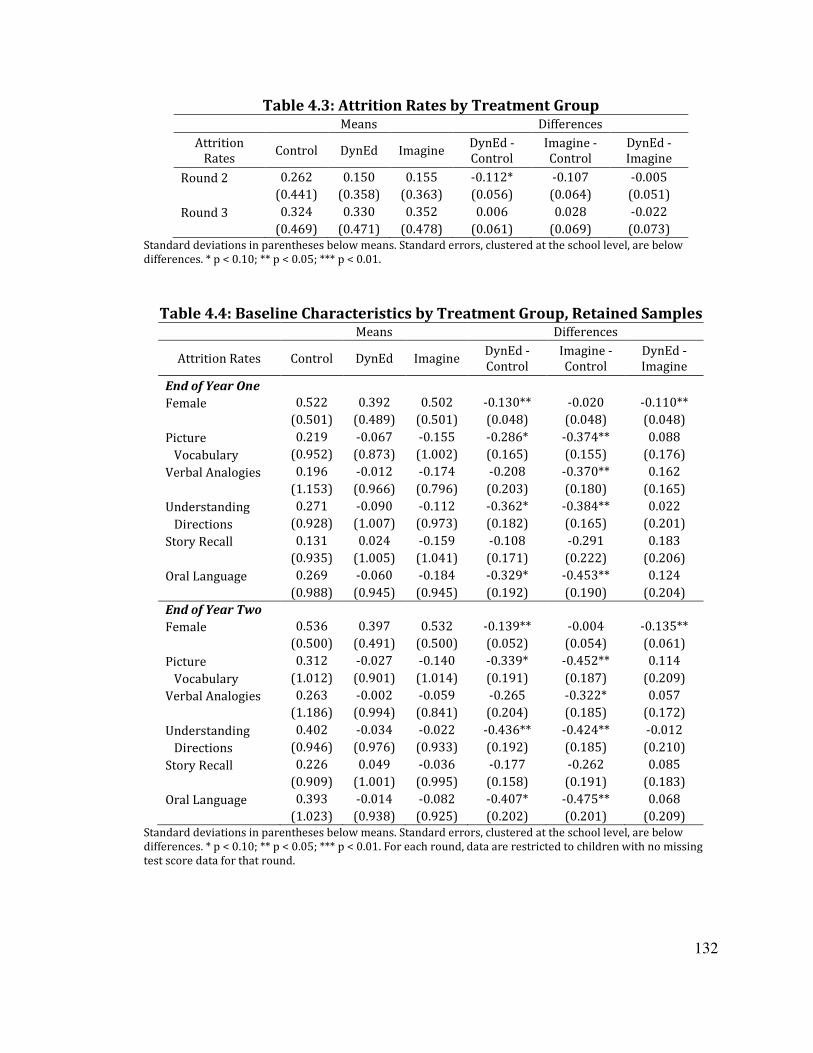
132

Table 4.3: Attrition Rates by Treatment Group Means Differences

Attrition Rates Control DynEd Imagine DynEd -

Control Imagine - Control

DynEd - Imagine

Round 2 0.262 0.150 0.155 -0.112* -0.107 -0.005 (0.441) (0.358) (0.363) (0.056) (0.064) (0.051) Round 3 0.324 0.330 0.352 0.006 0.028 -0.022 (0.469) (0.471) (0.478) (0.061) (0.069) (0.073)

Standard deviations in parentheses below means. Standard errors, clustered at the school level, are below differences. * p < 0.10; ** p < 0.05; *** p < 0.01.

Table 4.4: Baseline Characteristics by Treatment Group, Retained Samples Means Differences

Attrition Rates Control DynEd Imagine DynEd - Control

Imagine - Control

DynEd - Imagine

End of Year One Female 0.522 0.392 0.502 -0.130** -0.020 -0.110** (0.501) (0.489) (0.501) (0.048) (0.048) (0.048) Picture 0.219 -0.067 -0.155 -0.286* -0.374** 0.088 Vocabulary (0.952) (0.873) (1.002) (0.165) (0.155) (0.176) Verbal Analogies 0.196 -0.012 -0.174 -0.208 -0.370** 0.162 (1.153) (0.966) (0.796) (0.203) (0.180) (0.165) Understanding 0.271 -0.090 -0.112 -0.362* -0.384** 0.022 Directions (0.928) (1.007) (0.973) (0.182) (0.165) (0.201) Story Recall 0.131 0.024 -0.159 -0.108 -0.291 0.183 (0.935) (1.005) (1.041) (0.171) (0.222) (0.206) Oral Language 0.269 -0.060 -0.184 -0.329* -0.453** 0.124 (0.988) (0.945) (0.945) (0.192) (0.190) (0.204) End of Year Two Female 0.536 0.397 0.532 -0.139** -0.004 -0.135** (0.500) (0.491) (0.500) (0.052) (0.054) (0.061) Picture 0.312 -0.027 -0.140 -0.339* -0.452** 0.114 Vocabulary (1.012) (0.901) (1.014) (0.191) (0.187) (0.209) Verbal Analogies 0.263 -0.002 -0.059 -0.265 -0.322* 0.057 (1.186) (0.994) (0.841) (0.204) (0.185) (0.172) Understanding 0.402 -0.034 -0.022 -0.436** -0.424** -0.012 Directions (0.946) (0.976) (0.933) (0.192) (0.185) (0.210) Story Recall 0.226 0.049 -0.036 -0.177 -0.262 0.085 (0.909) (1.001) (0.995) (0.158) (0.191) (0.183) Oral Language 0.393 -0.014 -0.082 -0.407* -0.475** 0.068 (1.023) (0.938) (0.925) (0.202) (0.201) (0.209)

Standard deviations in parentheses below means. Standard errors, clustered at the school level, are below differences. * p < 0.10; ** p < 0.05; *** p < 0.01. For each round, data are restricted to children with no missing test score data for that round.

133

Table 4.5: Unadjusted Test Scores by Group, all Time Periods Control DynEd Imagine

Panel A: Baseline Picture Vocabulary 0.257 0.009 -0.102 Verbal Analogies 0.272 0.037 -0.120 Understanding Directions 0.368 0.008 0.003 Story Recall 0.176 0.068 -0.022 Oral Language Composite 0.350 0.029 -0.070

Panel B: End of Year One Picture Vocabulary 0.923 1.144 0.625 Verbal Analogies 0.416 0.204 0.167 Understanding Directions 0.783 1.014 0.469 Story Recall 0.833 0.665 0.676 Oral Language Composite 0.956 1.027 0.626

Panel C: End of Year Two Picture Vocabulary 1.276 1.338 0.957 Verbal Analogies 0.710 0.424 0.415 Understanding Directions 1.143 1.175 0.787 Story Recall 1.207 1.039 1.149 Oral Language Composite 1.396 1.318 1.055

All test scores are standardized by baseline test scores. The sample is restricted to the sample of children with test score data for all three rounds.

134

Table 4.6a: Treatment Effects – DynEd vs. Control Panel A: End of Year One (n=333)

Variables Picture Vocabulary

Verbal Analogies

Und. Directions

Story Recall

Oral Language

Constant 0.257** 0.272 0.368*** 0.176 0.350** (0.105) (0.177) (0.110) (0.134) (0.136) t 0.666*** 0.145 0.415*** 0.657*** 0.607*** (0.115) (0.194) (0.099) (0.170) (0.122) DynEd -0.248 -0.235 -0.360* -0.108 -0.320 (0.182) (0.228) (0.195) (0.172) (0.207) DynEd*t 0.469*** 0.022 0.590*** -0.060 0.391** (0.156) (0.264) (0.163) (0.199) (0.178) R2 0.192 0.015 0.146 0.120 0.161

Panel B: End of Year Two (n=333)

Variables Picture Vocabulary

Verbal Analogies

Und. Directions

Story Recall

Oral Language

Constant 0.257** 0.272 0.368*** 0.176 0.350** (0.105) (0.177) (0.110) (0.134) (0.136) t 1.019*** 0.438*** 0.775*** 1.031*** 1.046*** (0.101) (0.159) (0.083) (0.177) (0.128) DynEd -0.248 -0.235 -0.360* -0.108 -0.320 (0.182) (0.228) (0.195) (0.172) (0.207) DynEd*t 0.310* -0.051 0.392** -0.061 0.243 (0.160) (0.240) (0.162) (0.200) (0.175) R2 0.285 0.045 0.238 0.269 0.285

Sample is restricted to individuals without any missing test score data so that differences between the effects in the two rounds can be attributed to a difference in effects, not an evolving sample. Standard errors, reported in parentheses, are adjusted for school-level clustering. * p < 0.1; ** p < 0.05; *** p < 0.01.

135

Table 4.6b: Treatment Effects – Imagine Learning vs. Control Panel A: End of Year One (n=332)

Variables Picture Vocabulary

Verbal Analogies

Und. Directions

Story Recall

Oral Language

Constant 0.257** 0.272 0.368*** 0.176 0.350** (0.105) (0.176) (0.110) (0.134) (0.136) t 0.666*** 0.145 0.415*** 0.657*** 0.607*** (0.115) (0.194) (0.099) (0.170) (0.122) Imagine -0.359* -0.392* -0.365* -0.198 -0.420* (0.190) (0.203) (0.195) (0.209) (0.212) Imagine*t 0.061 0.142 0.051 0.041 0.090 (0.147) (0.238) (0.134) (0.218) (0.149) R2 0.128 0.031 0.078 0.141 0.130

Panel B: End of Year Two (n=332)

Variables Picture Vocabulary

Verbal Analogies

Und. Directions

Story Recall

Oral Language

Constant 0.257** 0.272 0.368*** 0.176 0.350** (0.105) (0.176) (0.110) (0.134) (0.136) t 1.019*** 0.438*** 0.775*** 1.031*** 1.046*** (0.101) (0.159) (0.083) (0.177) (0.128) Imagine -0.359* -0.392* -0.365* -0.198 -0.420* (0.190) (0.203) (0.195) (0.209) (0.212) Imagine*t 0.040 0.097 0.009 0.140 0.079 (0.140) (0.200) (0.122) (0.226) (0.154) R2 0.216 0.065 0.174 0.322 0.250

Sample is restricted to individuals without any missing test score data so that differences between the effects in the two rounds can be attributed to a difference in effects, not an evolving sample. Standard errors, reported in parentheses, are adjusted for school-level clustering. * p < 0.1; ** p < 0.05; *** p < 0.01.

136

Table 4.6c: Treatment Effects – DynEd vs. Imagine Learning

Panel A: End of Year One (n=331)

Variables Picture Vocabulary

Verbal Analogies

Und. Directions

Story Recall

Oral Language

Constant -0.102 -0.120 0.003 -0.022 -0.070 (0.158) (1.000) (0.161) (0.160) (0.162) t 0.726*** 0.287** 0.466*** 0.698*** 0.696*** (0.092) (0.138) (0.090) (0.136) (0.086) DynEd 0.111 0.156 0.005 0.090 0.099 (0.217) (0.176) (0.228) (0.193) (0.225) DynEd*t 0.409*** -0.120 0.540*** -0.101 0.302* (0.140) (0.225) (0.157) (0.171) (0.155) R2 0.231 0.017 0.157 0.115 0.193

Panel B: End of Year Two (n=331)

Variables Picture Vocabulary

Verbal Analogies

Und. Directions

Story Recall

Oral Language

Constant -0.102 -0.120 0.003 -0.022 -0.070 (0.158) (0.0996) (0.161) (0.160) (0.162) t 1.059*** 0.535*** 0.784*** 1.171*** 1.125*** (0.097) (0.121) (0.090) (0.141) (0.085) DynEd 0.111 0.156 0.005 0.090 0.099 (0.217) (0.176) (0.228) (0.193) (0.225) DynEd*t 0.270* -0.148 0.383** -0.201 0.163 (0.158) (0.217) (0.166) (0.168) (0.147) R2 0.289 0.052 0.225 0.284 0.298

Sample is restricted to individuals without any missing test score data so that differences between the effects in the two rounds can be attributed to a difference in effects, not an evolving sample. Standard errors, reported in parentheses, are adjusted for school-level clustering. * p < 0.1; ** p < 0.05; *** p < 0.01.

137

Table 4.7a: Effects of DynEd vs. Control for Low-Scoring Schools Panel A: End of Year One (n=333)

Variables Picture Vocabulary

Verbal Analogies

Und. Directions Story Recall Oral

Language

Constant 0.494*** 0.631*** 0.642*** 0.424*** 0.695*** (0.135) (0.216) (0.123) (0.109) (0.152) t 0.653*** -0.138 0.242** 0.403** 0.400*** (0.136) (0.264) (0.099) (0.170) (0.133) DynEd -0.023 -0.206 -0.130 -0.060 -0.129 (0.202) (0.306) (0.204) (0.136) (0.204) t*DynEd 0.274 0.100 0.500*** -0.005 0.318 (0.183) (0.393) (0.178) (0.218) (0.213) Low school -0.638*** -0.967*** -0.736*** -0.669** -0.930*** (0.164) (0.244) (0.159) (0.268) (0.178) t*Low 0.0344 0.762** 0.467** 0.683* 0.557** (0.251) (0.314) (0.204) (0.355) (0.244) DynEd*Low -0.370 0.120 -0.362 0.022 -0.242 (0.249) (0.337) (0.268) (0.318) (0.258) t*DynEd*Low 0.420 -0.314 0.109 -0.249 0.0549 (0.319) (0.472) (0.318) (0.406) (0.346) R2 0.304 0.102 0.271 0.183 0.312

Panel B: End of Year Two (n=333)

Variables Picture Vocabulary

Verbal Analogies

Und. Directions Story Recall Oral

Language

Constant 0.494*** 0.631*** 0.642*** 0.424*** 0.695*** (0.135) (0.216) (0.123) (0.109) (0.152) t 0.942*** 0.205 0.642*** 0.732*** 0.831*** (0.130) (0.188) (0.080) (0.154) (0.133) DynEd -0.023 -0.206 -0.130 -0.060 -0.129 (0.202) (0.306) (0.204) (0.136) (0.204) t*DynEd 0.156 0.022 0.138 0.038 0.133 (0.217) (0.359) (0.156) (0.182) (0.195) Low school -0.638*** -0.967*** -0.736*** -0.669** -0.930*** (0.164) (0.244) (0.159) (0.268) (0.178) t*Low 0.207 0.628** 0.359** 0.805** 0.580** (0.198) (0.292) (0.178) (0.351) (0.244) DynEd*Low -0.370 0.120 -0.362 0.022 -0.242 (0.249) (0.337) (0.268) (0.318) (0.258) t*DynEd*Low 0.298 -0.278 0.487 -0.368 0.129 (0.295) (0.452) (0.294) (0.391) (0.317) R2 0.376 0.135 0.351 0.327 0.411

Test scores are standardized using the full sample baseline test score means and standard deviations. This analysis is restricted to students with no missing test score data. Standard errors, adjusted for school-level clustering, are presented in parentheses. * p<.1; ** p<.05; *** p<.01.

138

Table 4.7b:

Effects of Imagine Learning vs. Control for Low-Scoring Schools Panel A: End of Year One (n=332)

Variables Picture Vocabulary

Verbal Analogies

Und. Directions Story Recall Oral

Language

Constant 0.494*** 0.631*** 0.642*** 0.424*** 0.695*** (0.135) (0.216) (0.123) (0.109) (0.152) t 0.653*** -0.138 0.242** 0.403** 0.400*** (0.136) (0.264) (0.099) (0.169) (0.133) Imagine -0.071 -0.474* -0.130 -0.077 -0.217 (0.224) (0.239) (0.184) (0.161) (0.197) t*Imagine -0.117 0.398 0.014 0.085 0.088 (0.169) (0.345) (0.135) (0.221) (0.152) Low school -0.638*** -0.967*** -0.736*** -0.669** -0.930*** (0.164) (0.244) (0.159) (0.268) (0.178) t*Low 0.034 0.762** 0.467** 0.683* 0.557** (0.251) (0.314) (0.204) (0.355) (0.244) Imagine*Low -0.471* 0.383 -0.340 -0.112 -0.230 (0.260) (0.289) (0.254) (0.382) (0.261) t*Imagine*Low 0.369 -0.704* -0.022 -0.240 -0.116 (0.304) (0.415) (0.254) (0.438) (0.286) R2 0.259 0.108 0.211 0.223 0.290

Panel B: End of Year Two (n=332)

Variables Picture Vocabulary

Verbal Analogies

Und. Directions Story Recall Oral

Language

Constant 0.494*** 0.631*** 0.642*** 0.424*** 0.695*** (0.135) (0.216) (0.123) (0.109) (0.152) t 0.942*** 0.205 0.642*** 0.732*** 0.831*** (0.130) (0.188) (0.080) (0.154) (0.133) Imagine -0.071 -0.474* -0.130 -0.077 -0.217 (0.224) (0.239) (0.184) (0.161) (0.197) t*Imagine 0.085 0.341 0.047 0.184 0.188 (0.162) (0.271) (0.147) (0.222) (0.170) Low school -0.638*** -0.967*** -0.736*** -0.669** -0.930*** (0.164) (0.244) (0.159) (0.268) (0.178) t*Low 0.207 0.628** 0.359** 0.805** 0.580** (0.198) (0.292) (0.178) (0.351) (0.244) Imagine*Low -0.471* 0.383 -0.340 -0.112 -0.230 (0.260) (0.289) (0.254) (0.382) (0.261) t*Imagine*Low -0.139 -0.650* -0.158 -0.266 -0.355 (0.282) (0.377) (0.247) (0.433) (0.294) R2 0.345 0.142 0.324 0.394 0.398

Test scores are standardized using the full sample baseline test score means and standard deviations. This analysis is restricted to students with no missing test score data. Standard errors, adjusted for school-level clustering, are presented in parentheses. * p<.1; ** p<.05; *** p<.01.

139

Table 4.7c: Effects of DynEd vs. Imagine Learning for Low-Scoring Schools

Panel A: End of Year One (n=331)

Variables Picture Vocabulary

Verbal Analogies

Und. Directions Story Recall Oral

Language

Constant 0.422** 0.156 0.512*** 0.347*** 0.478*** (0.179) (0.103) (0.137) (0.118) (0.125) t 0.536*** 0.260 0.256*** 0.489*** 0.488*** (0.100) (0.221) (0.092) (0.141) (0.073) DynEd 0.048 0.268 -0.001 0.017 0.088 (0.234) (0.240) (0.213) (0.144) (0.184) t*DynEd 0.391** -0.298 0.486*** -0.091 0.230 (0.158) (0.365) (0.174) (0.197) (0.182) Low school -1.109*** -0.584*** -1.076*** -0.780*** -1.160*** (0.202) (0.154) (0.198) (0.272) (0.191) t*Low 0.403** 0.058 0.445*** 0.442* 0.441*** (0.171) (0.272) (0.152) (0.257) (0.149) DynEd*Low 0.101 -0.263 -0.023 0.134 -0.012 (0.276) (0.279) (0.292) (0.321) (0.267) t*DynEd*Low 0.051 0.390 0.131 -0.008 0.171 (0.260) (0.445) (0.287) (0.323) (0.287) R2 0.405 0.113 0.328 0.196 0.405

Panel B: End of Year Two (n=331)

Variables Picture Vocabulary

Verbal Analogies

Und. Directions Story Recall Oral

Language

Constant 0.422** 0.156 0.512*** 0.347*** 0.478*** (0.179) (0.103) (0.137) (0.118) (0.125) t 1.027*** 0.545*** 0.689*** 0.917*** 1.019*** (0.097) (0.195) (0.124) (0.160) (0.105) DynEd 0.048 0.268 -0.001 0.017 0.088 (0.234) (0.240) (0.213) (0.144) (0.184) t*DynEd 0.072 -0.318 0.091 -0.146 -0.055 (0.199) (0.363) (0.182) (0.187) (0.178) Low school -1.109*** -0.584*** -1.076*** -0.780*** -1.160*** (0.202) (0.154) (0.198) (0.272) (0.191) t*Low 0.068 -0.022 0.201 0.539** 0.225 (0.201) (0.239) (0.171) (0.253) (0.164) DynEd*Low 0.101 -0.263 -0.023 0.134 -0.012 (0.276) (0.279) (0.292) (0.321) (0.267) t*DynEd*Low 0.436 0.372 0.645** -0.101 0.484* (0.297) (0.420) (0.290) (0.306) (0.261) R2 0.459 0.147 0.399 0.353 0.486

Test scores are standardized using the full sample baseline test score means and standard deviations. This analysis is restricted to students with no missing test score data. Standard errors, adjusted for school-level clustering, are presented in parentheses. * p<.1; ** p<.05; *** p<.01.

140

Table 4.8a: Effects of DynEd vs. Control for Low-Scoring Students Panel A: End of Year One (n=333)

Variables Picture Vocabulary

Verbal Analogies

Understanding Directions Story Recall Oral

Language Constant 0.872*** 1.375*** 0.885*** 0.902*** 0.927*** (0.095) (0.192) (0.084) (0.065) (0.127) t 0.387*** -0.740*** 0.202** 0.052 0.363*** (0.131) (0.246) (0.087) (0.138) (0.112) DynEd -0.149 -0.224 -0.070 0.008 -0.136 (0.137) (0.262) (0.139) (0.089) (0.167) t*DynEd 0.327* 0.0519 0.239 -0.138 0.141 (0.163) (0.371) (0.151) (0.199) (0.192) Low -1.533*** -2.002*** -1.487*** -1.348*** -1.506*** (0.093) (0.192) (0.105) (0.143) (0.135) t*Low 0.695*** 1.606*** 0.615*** 1.122*** 0.637*** (0.142) (0.226) (0.178) (0.236) (0.178) DynEd*Low -0.005 0.224 -0.146 -0.206 -0.036 (0.143) (0.262) (0.175) (0.179) (0.187) t*DynEd*Low 0.213 -0.241 0.529** 0.137 0.365 (0.231) (0.364) (0.255) (0.293) (0.270) R2 0.507 0.369 0.490 0.434 0.481

Panel B: End of Year Two (n=333)

Variables Picture Vocabulary

Verbal Analogies

Understanding Directions Story Recall Oral

Language Constant 0.872*** 1.375*** 0.885*** 0.902*** 0.927*** (0.095) (0.192) (0.084) (0.065) (0.127) t 0.782*** -0.408** 0.514*** 0.408*** 0.756*** (0.106) (0.160) (0.085) (0.084) (0.110) DynEd -0.149 -0.224 -0.070 0.008 -0.136 (0.137) (0.262) (0.139) (0.089) (0.167) t*DynEd 0.148 -0.208 0.038 0.025 0.065 (0.178) (0.274) (0.155) (0.107) (0.165) Low -1.533*** -2.002*** -1.487*** -1.348*** -1.506*** (0.093) (0.192) (0.105) (0.143) (0.135) t*Low 0.590*** 1.536*** 0.751*** 1.156*** 0.756*** (0.134) (0.200) (0.182) (0.222) (0.165) DynEd*Low -0.005 0.224 -0.146 -0.206 -0.036 (0.143) (0.262) (0.175) (0.179) (0.187) t*DynEd*Low 0.270 0.066 0.495* -0.165 0.191 (0.200) (0.306) (0.256) (0.265) (0.226) R2 0.584 0.380 0.553 0.567 0.557

Test scores are standardized using the full sample baseline test score means and standard deviations. This analysis is restricted to students with no missing test score data. Standard errors, adjusted for school-level clustering, are presented in parentheses. * p<.1; ** p<.05; *** p<.01.

141

Table 4.8b: Effects of Imagine Learning vs. Control for Low-Scoring Students

Panel A: End of Year One (n=332)

Variables Picture Vocabulary

Verbal Analogies

Understanding Directions Story Recall Oral

Language Constant 0.872*** 1.375*** 0.885*** 0.902*** 0.927*** (0.095) (0.192) (0.084) (0.065) (0.127) t 0.387*** -0.740*** 0.202** 0.052 0.363*** (0.131) (0.246) (0.087) (0.138) (0.112) Imagine -0.053 -0.583*** -0.064 0.039 -0.166 (0.161) (0.213) (0.131) (0.087) (0.162) t*Imagine -0.134 0.391 -0.151 -0.065 -0.054 (0.181) (0.307) (0.122) (0.175) (0.166) Low -1.533*** -2.002*** -1.487*** -1.348*** -1.506*** (0.093) (0.192) (0.105) (0.143) (0.135) t*Low 0.695*** 1.606*** 0.615*** 1.122*** 0.637*** (0.142) (0.226) (0.178) (0.236) (0.178) Imagine*Low -0.155 0.583*** -0.159 -0.152 -0.088 (0.170) (0.213) (0.157) (0.202) (0.196) t*Imagine*Low 0.173 -0.615** 0.221 -0.016 0.107 (0.255) (0.289) (0.219) (0.276) (0.254) R2 0.475 0.341 0.458 0.433 0.480

Panel B: End of Year Two (n=332)

Variables Picture Vocabulary

Verbal Analogies

Understanding Directions Story Recall Oral

Language Constant 0.872*** 1.375*** 0.885*** 0.902*** 0.927*** (0.095) (0.192) (0.084) (0.065) (0.127) t 0.782*** -0.408** 0.514*** 0.408*** 0.756*** (0.106) (0.160) (0.085) (0.084) (0.110) Imagine -0.053 -0.583*** -0.064 0.039 -0.166 (0.161) (0.213) (0.131) (0.087) (0.162) t*Imagine -0.011 0.560** -0.078 -0.002 0.118 (0.186) (0.214) (0.153) (0.148) (0.190) Low -1.533*** -2.002*** -1.487*** -1.348*** -1.506*** (0.093) (0.192) (0.105) (0.143) (0.135) t*Low 0.590*** 1.536*** 0.751*** 1.156*** 0.756*** (0.134) (0.200) (0.182) (0.221) (0.165) Imagine*Low -0.155 0.583*** -0.159 -0.152 -0.088 (0.170) (0.213) (0.157) (0.202) (0.196) t*Imagine*Low -0.061 -0.940*** -0.050 0.035 -0.274 (0.226) (0.251) (0.235) (0.268) (0.233) R2 0.545 0.368 0.533 0.583 0.555

Test scores are standardized using the full sample baseline test score means and standard deviations. This analysis is restricted to students with no missing test score data. Standard errors, adjusted for school-level clustering, are presented in parentheses. * p<.1; ** p<.05; *** p<.01.

142

Table 4.8c: Effects of DynEd vs. Imagine for Low-Scoring Students Panel A: End of Year One (n=331)

Variables Picture Vocabulary

Verbal Analogies

Understanding Directions

Story Recall

Oral Language

Constant 0.819*** 0.792*** 0.821*** 0.941*** 0.761*** (0.130) (0.093) (0.101) (0.058) (0.100) t 0.253** -0.350* 0.051 -0.013 0.309** (0.125) (0.184) (0.085) (0.108) (0.122) DynEd -0.096 0.358* -0.006 -0.031 0.030 (0.163) (0.200) (0.150) (0.084) (0.148) t*DynEd 0.461*** -0.339 0.390** -0.073 0.194 (0.158) (0.333) (0.150) (0.179) (0.198) Low -1.688*** -1.420*** -1.646*** -1.499*** -1.594*** (0.142) (0.093) (0.117) (0.142) (0.141) t*Low 0.867*** 0.991*** 0.836*** 1.106*** 0.744*** (0.211) (0.179) (0.129) (0.143) (0.180) DynEd*Low 0.150 -0.358* 0.013 -0.054 0.052 (0.179) (0.200) (0.183) (0.178) (0.192) t*DynEd*Low 0.040 0.374 0.307 0.153 0.258 (0.279) (0.337) (0.223) (0.224) (0.271) R2 0.589 0.349 0.512 0.435 0.549

Panel B: End of Year Two (n=331)

Variables Picture Vocabulary

Verbal Analogies

Understanding Directions

Story Recall

Oral Language

Constant 0.819*** 0.792*** 0.821*** 0.941*** 0.761*** (0.130) (0.093) (0.101) (0.058) (0.100) t 0.770*** 0.152 0.436*** 0.406*** 0.874*** (0.153) (0.142) (0.127) (0.122) (0.155) DynEd -0.096 0.358* -0.006 -0.031 0.030 (0.163) (0.200) (0.150) (0.084) (0.148) t*DynEd 0.160 -0.768*** 0.116 0.0271 -0.053 (0.210) (0.264) (0.182) (0.139) (0.198) Low -1.688*** -1.420*** -1.646*** -1.499*** -1.594*** (0.142) (0.093) (0.117) (0.142) (0.141) t*Low 0.529*** 0.597*** 0.701*** 1.191*** 0.482*** (0.182) (0.152) (0.148) (0.152) (0.165) DynEd*Low 0.150 -0.358* 0.0134 -0.054 0.052 (0.179) (0.200) (0.183) (0.178) (0.192) t*DynEd*Low 0.331 1.006*** 0.545** -0.200 0.465** (0.236) (0.277) (0.233) (0.210) (0.226) R2 0.623 0.365 0.577 0.583 0.621

Test scores are standardized using the full sample baseline test score means and standard deviations. This analysis is restricted to students with no missing test score data. Standard errors, adjusted for school-level clustering, are presented in parentheses. * p<.1; ** p<.05; *** p<.01.

143

Table 4.9a: Effects of DynEd vs. Control by Gender Panel A: End of Year One (n=333)

Variables Picture Vocabulary

Verbal Analogies

Und. Directions

Story Recall

Oral Language

Constant 0.257* 0.283 0.384*** 0.166 0.353** (0.128) (0.201) (0.136) (0.175) (0.153) t 0.595*** 0.060 0.349*** 0.577*** 0.515*** (0.140) (0.247) (0.119) (0.196) (0.134) DynEd -0.189 -0.242 -0.259 -0.068 -0.248 (0.198) (0.263) (0.219) (0.213) (0.224) t*DynEd 0.576*** 0.114 0.590*** -0.029 0.457** (0.187) (0.308) (0.187) (0.220) (0.192) Female -0.000 -0.021 -0.030 0.018 -0.006 (0.163) (0.170) (0.156) (0.142) (0.149) t*Female 0.132 0.158 0.124 0.148 0.170 (0.157) (0.254) (0.157) (0.187) (0.147) DynEd*Female -0.149 0.0102 -0.264 -0.094 -0.185 (0.225) (0.260) (0.237) (0.173) (0.221) t*DynEd*Female -0.222 -0.174 0.044 -0.027 -0.105 (0.267) (0.365) (0.241) (0.207) (0.247) R2 0.197 0.016 0.153 0.122 0.166

Panel A: End of Year Two (n=333)

Variables Picture Vocabulary

Verbal Analogies

Und. Directions

Story Recall

Oral Language

Constant 0.257* 0.283 0.384*** 0.166 0.353** (0.128) (0.201) (0.136) (0.175) (0.153) t 1.007*** 0.371* 0.700*** 1.041*** 1.001*** (0.125) (0.201) -0.077 (0.217) (0.127) DynEd -0.189 -0.242 -0.259 -0.068 -0.248 (0.198) (0.263) (0.219) (0.213) (0.224) t*DynEd 0.246 0.038 0.337* -0.064 0.217 (0.195) (0.284) (0.170) (0.242) (0.185) Female school 0.000 -0.021 -0.03 0.018 -0.006 (0.163) (0.170) (0.156) (0.142) (0.149) t*Female 0.021 0.123 0.139 -0.018 0.083 (0.128) (0.280) (0.121) (0.242) (0.172) DynEd*Female -0.149 0.01 -0.264 -0.094 -0.185 (0.225) (0.260) (0.237) (0.173) (0.221) t*DynEd*Female 0.169 -0.178 0.188 0.003 0.093 (0.182) (0.361) (0.202) (0.281) (0.220) R2 0.286 0.045 0.244 0.269 0.287

Test scores are standardized using the full sample baseline test score means and standard deviations. This analysis is restricted to students with no missing test score data. Standard errors, adjusted for school-level clustering, are presented in parentheses. * p<.1; ** p<.05; *** p<.01.

144

Table 4.9b: Effects of Imagine Learning vs. Control by Gender Panel A: End of Year One (n=332)

Variables Picture Vocabulary

Verbal Analogies

Und. Directions

Story Recall

Oral Language

Constant 0.257** 0.283 0.384*** 0.166 0.353** (0.128) (0.201) (0.136) (0.175) (0.153) t 0.595*** 0.060 0.349*** 0.577*** 0.515*** (0.140) (0.247) (0.119) (0.196) (0.134) Imagine -0.393** -0.458** -0.383 -0.133 -0.434* (0.193) (0.222) (0.228) (0.239) (0.223) t*Imagine 0.232 0.445 0.223 0.124 0.310* (0.184) (0.292) (0.200) (0.246) (0.182) Female 0.000 -0.021 -0.030 0.018 -0.006 (0.163) (0.170) (0.156) (0.142) (0.149) t*Female 0.132 0.158 0.124 0.148 0.170 (0.157) (0.254) (0.157) (0.187) (0.147) Imagine*Female 0.065 0.125 0.033 -0.123 0.028 (0.213) (0.194) (0.221) (0.220) (0.202) t*Imagine*Female -0.322 -0.571* -0.324 -0.154 -0.413* (0.213) (0.300) (0.252) (0.263) (0.210) R2 0.130 0.037 0.081 0.145 0.134

Panel A: End of Year Two (n=332)

Variables Picture Vocabulary

Verbal Analogies

Und. Directions

Story Recall

Oral Language

Constant 0.257** 0.283 0.384*** 0.166 0.353** (0.128) (0.201) (0.136) (0.175) (0.153) t 1.007*** 0.371* 0.700*** 1.041*** 1.001*** (0.125) (0.201) (0.077) (0.217) (0.127) DynEd -0.393** -0.458** -0.383 -0.133 -0.434* (0.193) (0.222) (0.228) (0.239) (0.223) t*DynEd 0.174 0.370 0.121 0.139 0.237 (0.171) (0.254) (0.162) (0.265) (0.177) Female -0.000 -0.021 -0.030 0.018 -0.006 (0.163) (0.170) (0.156) (0.142) (0.149) t*Female 0.021 0.123 0.139 -0.018 0.083 (0.128) (0.280) (0.121) (0.242) (0.172) DynEd*Female 0.065 0.125 0.033 -0.123 0.028 (0.213) (0.194) (0.221) (0.220) (0.202) t*DynEd*Female -0.254 -0.515 -0.209 0.001 -0.297 (0.196) (0.321) (0.211) (0.290) (0.228) R2 0.217 0.070 0.175 0.324 0.252

Test scores are standardized using the full sample baseline test score means and standard deviations. This analysis is restricted to students with no missing test score data. Standard errors, adjusted for school-level clustering, are presented in parentheses. * p<.1; ** p<.05; *** p<.01.

145

Table 4.9c: Effects of DynEd vs. Imagine Learning for Low-Performing Schools Panel A: End of Year One (n=331)

Variables Picture Vocabulary

Verbal Analogies

Und. Directions

Story Recall

Oral Language

Constant -0.136 -0.175* 0.001 0.033 -0.081 (0.145) -0.096 (0.184) (0.163) (0.162) t 0.826*** 0.505*** 0.572*** 0.701*** 0.825*** (0.119) (0.156) (0.161) (0.148) (0.123) DynEd 0.204 0.216 0.124 0.065 0.187 (0.209) (0.195) (0.252) (0.203) (0.230) t*DynEd 0.344* -0.332 0.367* -0.153 0.147 (0.172) (0.241) (0.216) (0.178) (0.185) Female 0.065 0.104 0.003 -0.105 0.022 (0.137) -0.094 (0.156) (0.168) (0.136) t*Female -0.190 -0.414** -0.200 -0.006 -0.243 (0.144) (0.159) (0.197) (0.184) (0.150) DynEd*Female -0.214 -0.115 -0.297 0.029 -0.213 (0.207) (0.218) (0.237) (0.195) (0.212) t*DynEd*Female 0.099 0.397 0.368 0.127 0.308 (0.259) (0.307) (0.269) (0.204) (0.249) R2 0.237 0.024 0.164 0.117 0.199

Panel A: End of Year Two (n=331)

Variables Picture Vocabulary

Verbal Analogies

Und. Directions

Story Recall

Oral Language

Constant -0.136 -0.175* 0.001 0.033 -0.081 (0.145) -0.096 (0.184) (0.163) (0.162) t 1.182*** 0.741*** 0.821*** 1.180*** 1.238*** (0.116) (0.156) (0.142) (0.153) (0.123) DynEd 0.204 0.216 0.124 0.065 0.187 (0.209) (0.195) (0.252) (0.203) (0.230) t*DynEd 0.072 -0.332 0.216 -0.204 -0.020 (0.190) (0.254) (0.208) (0.186) (0.182) Female 0.065 0.104 0.003 -0.105 0.022 (0.137) -0.094 (0.156) (0.168) (0.136) t*Female -0.233 -0.391** -0.070 -0.017 -0.214 (0.149) (0.157) (0.173) (0.159) (0.149) DynEd*Female -0.214 -0.115 -0.297 0.029 -0.213 (0.207) (0.218) (0.237) (0.195) (0.212) t*DynEd*Female 0.424** 0.336 0.397* 0.002 0.390* (0.197) (0.277) (0.237) (0.213) (0.203) R2 0.291 0.057 0.230 0.287 0.301

Test scores are standardized using the full sample baseline test score means and standard deviations. This analysis is restricted to students with no missing test score data. Standard errors, adjusted for school-level clustering, are presented in parentheses. * p<.1; ** p<.05; *** p<.01.

146

Chapter 5: Conclusion

147

This dissertation presents the results of three field experiments that were

implemented to evaluate the effectiveness of public policies or programs designed

to improve health or educational outcomes of children in Latin America. This

research contributes to a rapidly growing body of knowledge on what works to

develop children’s human capital in developing countries. This work also

contributes to the growing body of research on how to take advantage of increasing

access to technology for development.

Chapter 2 showed that a low-cost intervention that delivers timely and

concise information to community health workers can improve take-up of

preventive care services. This type of intervention could easily be scaled up within

Guatemala, and has potential to be replicated in other countries with similar

programs. Future research should evaluate the viability and effectiveness of sending

vaccination reminders to parents as well as or instead of to community health

workers. The electronic medical record system used in the PEC and other similar

programs has the potential to facilitate other low-cost interventions. In the future, it

would also be worthwhile to evaluate the viability and effectiveness of adding

performance feedback to patient tracking lists as a strategy to increase community

health worker motivation.

Chapter 3 presented the results of a field experiment that did not have

detectable effects. Intensive teacher training on the use of the One Laptop Per Child

laptops did not increase teachers’ or students’ use of the laptops or student test

scores, nor did it improve teachers’ or students’ opinions of the laptops. Teachers in

Peru have expressed a desire for more training, yet this training was not enough to

148

lead to meaningful behavior change. It seems unlikely that this type of training

would achieve the goal of making the laptop program effective.

While the results presented in Chapter 3 do not inspire much enthusiasm for

technology as an educational tool, the research on software for English language

learning in Costa Rica presented in Chapter 4 shows that technology can be

effective. Comparing the experiences in Peru and Costa Rica, it is clear that

technology has diverse effects in education. It is no silver bullet, but it does have the

potential to improve learning.

One characteristic that may have driven the DynEd software’s strong effects

was that it was highly structured; it did not require significant teacher training, or

teacher expertise on how to integrate the software into an existing curriculum. The

software’s effectiveness regardless of teacher skill is made clear by the fact that the

software was effective even though half the schools that used it were not likely to

have had an English teacher. This is in sharp contrast to the One Laptop Per Child

program, which was designed with the expectation that teachers and students

would discover how to use the computers, and how to integrate them into the

curriculum on their own. Software interventions may be more effective when they

are highly structured, particularly if they are designed to compensate for

weaknesses in teachers’ abilities.

As was mentioned in Chapter 1, financial commitments to development are

not enough to improve health or education outcomes. Policy-makers need reliable

information on what works in education, health and other fields to make the most of

the scarce resources they have to tackle enormous and pressing challenges. This

149

research has been an attempt to support policy-makers in these efforts.

150

Bibliography

Angrist, J. & Lavy, V. (2002). New Evidence on Classroom Computers and Pupil

Learning. The Economic Journal 112 (October), 735-765. Angrist, J. & Pischke, J. (2009). Mostly Harmless Econometrics. Princeton: Princeton

University Press. Atikinson, W., Pickering L., Schwartz, B., Weniger, B., Iskander, J., & Watson, J.

(2002). General recommendations on immunization. Morbidity and Mortality Weekly Report (MMWR) 51(No. RR-2), 1-36.

Banerjee, A., Cole, S., Duflo, E. & Linden, L. (2007). Remedying Education: Evidence

from Two Randomized Experiments in India. The Quarterly Journal of Economics 122(3), 1235-1264.

Banerjee, A., Deaton, A. and Duflo, E. (2004). Wealth, Health and Health Services in

Rural Rajasthan. American Economic Review 94(2), 326-330. Banerjee A, Deaton A, Duflo E. (2004). Health care delivery in rural Rajasthan.

Economic and Political Weekly; 39: 944–49. Banerjee, A., Duflo, E., Glennerster R., & D. Kothari. (2010). Improving Immunization

Coverage in Rural India: A Clustered Randomized Controlled Evaluation of Immunization Campaigns with and without Incentives. British Medical Journal 340. May 17.

Banerjee, A. & He, R. (2003). “The World Bank of the Future,” American Economic

Review, Papers and Proceedings, 93(2), 39-44. Barham, T. & Maluccio, J. (2010). Eradicating diseases: The effect of conditional cash

transfers on vaccination coverage in rural Nicaragua. Journal of Health Economics 28: 611-621.

Barrera-Osorio, F. & Linden L. (2009). The Use and Misuse of Computers in

Education. World Bank Policy Research Working Paper 4836, Impact Evaluation Series No. 29.

Barrett, C. & Carter, M. (2010). Powers and Pitfalls of Experiments in Development

Economics: Some Non-random Reflections. Applied Economic Perspectives and Policy 32(4), 515-548.

151

Barrow, L., Markman, L. & Rouse, C. (2007). Technology’s Edge: The Educational Benefits of Computer-Aided Instruction. Federal Reserve Bank of Chicago Working Paper 2007-17.

Becerra, O. (2012a). “Oscar Becerra on OLPC’s Long-Term Impact.” Educational

Technology Debate, March 13, 2012. Accessed online at https://edutechdebate.org/olpc-in-peru/oscar-becerra-on-olpc-perus-long-term-impact/ on June 20, 2013.

Becerra, O. (2012b). Personal interview in Lima, Peru. December 5. Beshears, J., Choi, J-J., Laibson, D. & Madrian, B-C. (2008). How are preferences

revealed? Journal of Public Economics 92, 1787-1794. Blaya, J., Fraser, H.S.F. & Holt, B. (2010). E-Health Technologies Show Promise in

Developing Countries. Health Affairs 29 (2), 244-251. Bloom, D., Canning, D., & Weston, M. (2005). The value of vaccination. World

Economics 6 (3), 15-39. British Broadcast Corporation (BBC) News. (2005). “UN Debut for $100 Laptop for

Poor.” November 17, 2005. Accessed online at http://news.bbc.co.uk/2/hi/technology/4445060.stm on June 10, 2013.

Bruhn, M. & McKenzie, D. (2009). In Pursuit of Balance: Randomization in Practice in

Development Field Experiments. American Economic Journal: Applied Economics 1(4), 200-232.

Campuzano, L., Dynarski, M., Agodini, R., & Rall, K. (2009). Effectiveness of Reading

and Mathematics Software Products: Findings From Two Student Cohorts—Executive Summary (NCEE 2009-4042). Washington, DC: National Center for Education Evaluation and Regional Assistance, Institute of Education Sciences, U.S. Department of Education.

Cristia, J., Evans, W. & Kim, B. (2011). Does Contracting-Out Primary Care Services

Work? The Case of Rural Guatemala. Inter-American Development Bank Working Paper 273.

Cristia, J., Ibarrarán, S., Cueto, S. , Santiago, A. & Severín, E. (2012). Technology and

Child Development: Evidence from the One Laptop Per Child Program. Inter-American Development Bank Working Paper 304.

DynEd International, Inc. (2013). “First English Progam Overview.” Accessed online

at http://www.dyned.com/us/products/firstenglish/ on April 10, 2013.

152

Dasgupta, P. & Maskin, E. (2005). Uncertainty and Hyperbolic Discounting. American Economic Review 95 (4), 1290-1299.

DellaVigna, S. (2009). Psychology and Economics: Evidence from the Field. Journal of

Economic Literature 47 (2), 315-372 (June). DellaVigna, S., List, J., & Malmendier, U. (2012). Testing for Altruism and Social

Pressure in Charitable Giving. Quarterly Journal of Economics 127 (1): 1-57 (February).

Dirección General de Tecnologías Educativas, Ministerio de Educación de Perú.

(2010a). Plan “Acompañamiento Pedagógico del Programa Una Laptop Por Niño”. August 2010. Mimeographed document.

Dirección General de Tecnologías Educativas, Ministerio de Educación de Perú.

(2010b). Informe de Ejecución del Plan de Acompañamiento Pedagógico del Programa “Una Laptop Por Niño” en las II.EE. que forman parte de la evaluación realizada por el BID. October-December, 2010. Mimeographed document.

Duflo, E. (2004). “Scaling Up and Evaluation” in Accelerating Development, edited by

Francois Bourguignon and Boris Pleskovic. Oxford, UK and Washington, DC: Oxford University Press and World Bank.

Duflo, E., Glennerster, R., and Kremer, M. (2008). Using Randomization in

Development Economics Research: A Toolkit. Handbook of Development Economics, Vol. 4: 3895-3962.

The Economist. (2008). One clunky laptop per child. The Economist. January 4, 2008.

Accessed online at http://www.economist.com/node/10472304 on June 10, 2013.

The Economist. (2012). Error Message. The Economist. April 7, 2012. Accessed

online at http://www.economist.com/node/21552202 on July 2, 2013. Ferrando, M., Machado, A., Perazzo, I., & Haretche, C. (2010). Una primera

evaluación de los efectos del Plan Ceibal en base a datos de panel. Mimeograph accessed online at http://www.ccee.edu.uy/ensenian/catsemecnal/material/Ferrando_M.Machado_A.Perazzo_I.y_Vernengo_A.%282010%29.Evaluacion_de_impacto_del_Plan_Ceibal.pdf on June 10, 2013.

ENCOVI (Encuesta de Condiciones de Vida). (2009). Instituto Nacional de

Estadisticas de Guatemala.

153

ENSMI (Encuesta de Salud Materno-Infantil). (2011). Ministerio de Salud Pública y Asistencia Social de Guatemala.

Fernald, L., Gertler, P. & Neufeld, L. (2008). Role of cash in conditional cash transfer

programmes for child health, growth and development: an analysis of Mexico’s Oportunidades. The Lancet 371: 828-37.

Fiszbein, A., Schady, N. & Ferreira, F. (2009). Conditional Cash Transfers: Reducing

Present and Future Poverty. Washington, DC: The World Bank. Fudenberg, D., & Levine, D-K. (2006). A dual-self model of impulse control. American

Economic Review 96: 1449-1476. Glewwe, P., Hanushek, R., Humpage, S., & Ravina, R. (Forthcoming). School

Resources and Educational Outcomes in Developing Countries: A Review of the Literature From 1990 To 2010 in Education Policy in Developing Countries. Paul Glewwe, editor. Chicago, United States: University of Chicago Press.

Glewwe, P. & Kremer, M. (2006). “Schools, Teachers and Education Outcomes in

Developing Countries.” In: E. Hanushek and F. Welch, editors. Handbook of the Economics of Education. Amsterdam, The Netherlands: Elsevier.

Glewwe, P., Kremer, M. & Moulin, S. (2009). Many Children Left Behind? Textbooks

and Test Scores in Kenya. American Economic Journal: Applied Economics 1 (1), 112-135.

Greene, W. (2003). Econometric Analysis. New Jersey, Pearson Education. Fifth

Edition. Hansen, N., Koudenburg, N., Hiersemann, R., Tellegen, P. J., Kocsev, M. & Postmes, T.

(2012). Laptop usage affects abstract reasoning of children in the developing world. Computers & Education 59: 989-1000.

He, F., Linden, L. & MacLeod, M. (2007). Helping Teach What Teachers Don’t Know:

An Assessment of the Pratham English Language Learning Program. New York, United States: Columbia University. Mimeograph.

Heckman, J. (1979). Sample selection bias as a specification error. Econometrica 47

(1), 153-161. Imagine Learning, Inc. (2013). Program Overview. Accessed online at

http://www.imaginelearning.com/school/ProgramOverview.html on April 10, 2013.

154

Imbens, G. & Angrist, J. (1994). The Identification and Estimation of Local Average Treatment Effects. Econometrica 62(2), 467-76.

Instituto Nacional de Estadísticas y Censos (INEC). (2013). Datos del País. Accessed

online at http://www.inec.go.cr/Web/Home/pagPrincipal.aspx on July 6, 2013.

Instituto Nacional de Estadística e Informática (INEI). (2007). Censos Nacionales

2007: XI de Población y VI de Vivienda. Jacobson Vann, J. & Szilagyi, P. (2009). Patient Reminder and Recall Systems to

Improve Immunization Rates. Cochrane Database of Systematic Reviews 2005, Issue 3.

Lee, D.S. (2009). Training, Wages, and Sample Selection: Estimating Sharp Bounds

on Treatment Effects. Review of Economic Studies 76(3), 1071-1102. Leuven, E., Lindhal, M., Oosterbeek, H. & Webbink, D. (2004). The Effect of Extra

Funding for Disadvantaged Pupils on Achievement. IZA Discussion Paper Series No. 1122.

Linden, L. (2008). Complement or Substitute? The Effect of Technology on Student

Achievement in India. New York, United States: Columbia University. Mimeograph.

Loewenstein, G. (1992). “The Fall and Rise of Psychological Explanations in the

Economics of Intertemporal Choice,” in G. Loewenstein and J. Elder, eds., Choice Over Time. New York: Russell Sage Foundation, pp. 3-34.

Malamud, O., and C. Pop-Eleches. (2011). Home Computers and the Development of

Human Capital. Quarterly Journal of Economics 126: 987-1027. Ministerio de Educación Pública (MEP). (2013). Número de Instituciones y Servicios

Educativos en Educación Regular, Dependencia Pública, Privada y Privada Subvencionada. Accessed online at http://www.mep.go.cr/indica_educa/cifras_instituciones2.html on July 6, 2013.

Malamud, O., & Pop-Eleches, C. (2011). Home Computers and the Development of

Human Capital. Quarterly Journal of Economics 126: 987-1027. Manski, C.F. (1989). Schooling as experimentation: A reappraisal of the

postsecondary dropout phenomenon. Economics of Education Review 8 (4), 305-312.

155

Mullainathan, S. (2005). “Development Economics Through the Lens of Psychology” in Annual World Bank Conference in Development Economics 2005: Lessons of Experience, edited by Francois Bourguignon and Boris Pleskovic. Oxford, UK and Washington, DC: Oxford University Press and World Bank.

O’Donoghue, T., & Rabin, M. (1999). Doing it Now or Later. American Economic

Review 89: 103-124. One Laptop Per Child Foundation. (2013a). “One Laptop Per Child (OLPC), Project”.

Accessed online at http://laptop.org/en/vision/project/ on June 10, 2013. One Laptop Per Child Foundation. (2013b). “One Laptop Per Child: Countries.”

Accessed online at http://laptop.org/about/countries on June 10, 2013. One Laptop Per Child Foundation. (2013c). “OLPC: Five Principles”. Accessed online

at http://wiki.laptop.org/go/OLPC:Five_principles on June 10, 2013. One Laptop Per Child Foundation. (2013d). “One Laptop Per Child (OLPC): Project”.

Accessed online at http://one.laptop.org/about/software on June 11, 2013. One Laptop Per Child Foundation. (2013e). “One Laptop Per Child Wiki: Peru”.

Accessed online at http://wiki.laptop.org/go/OLPC_Peru on June 29, 201.3. One Laptop Per Child Foundation. (2013f). “One Laptop Per Child Map”. Website

accessed May 16, 2013 at laptop.org/map. Organization for Economic Cooperation and Development (OECD). (2013). DAC

Members’ Net Official Development Assistance in (2011). Accessed online at http://www.oecd.org/dataoecd/31/22/47452398.xls on July 10, 2013.

Partnership for Educational Revitalization in the Americas (PREAL). (2009). How

Much Are Latin American Children Learning? Highlights from the Second Regional Student Achievement Test (SERCE). Washington, DC, United States: Inter-American Dialogue.

Penuel, W. (2006). Implementation and Effects of One-to-One Computing Initiatives:

A Research Synthesis. Journal of Research on Technology in Education 38(3), 329-348.

Perkins, D., Radelet, S., Lindauer, D. and Block, S. 2013. Economics of Development.

New York, United States: W.W. Norton & Company. Seventh Edition. Pinon, R. & Haydon, J. (2010). English Language Quantitative Indicators: Cameroon,

Nigeria, Rwanda, Bangladesh and Pakistan. A custom report compiled by Euromonitor International for the British Council.

156

Programa Una Laptop Por Niño Peru. (2013). “Programa Una Laptop Por Niño”

webpage. Accessed online at http://www.perueduca.edu.pe/olpc/OLPC_programa.html on June 25, 2013.

Rosas, R., Nussbaum, M., Cumsille, P., Marianov, V., Correa, M., Flores, P. et al. (2003).

Beyond Nintendo: design and assessment of educational video games for first and second grade students. Computers and Education 40, 71-94.

Roschelle, J., Shechtman, N., Tatar, D., Hegedus, S., Hopkins, B., Empson, S. et al.

(2010). Integration of Technology, Curriculum, and Professional Development for Advancing Middle School Mathematics: Three Large-Scale Studies. American Educational Research Journal 47 (4), 833-878.

Rouse, C. & Kreuger, A. (2004). Putting Computerized Instruction to the Test: A

Randomized Evaluation of a “Scientifically Based” Reading Program. Economics of Education Review 23(4), 323-338.

Ryman T.K., Dietz, V. & Cairns, K.L. (2008). Too little but not too late: Results of a

literature review to improve routine immunization programs in developing countries. BMC Health Services Research 8:134.

Schultz, T. (1961). Investment in Human Capital. The American Economic Review

51(1), 1-17. Severin, E. & C. Capota. (2011). One-to-One Laptop Programs in Latin America and

the Caribbean: Panorama and Perspectives. Inter-American Development Bank Technical Note 261.

Sharma, U. (2012). “Essays on the Economics of Education in Developing Countries.”

Minneapolis, United States: University of Minnesota. Ph.D. dissertation. Shea, B., Andersson, N. & Henry, D. (2009). Increasing the demand for childhood

vaccination in developing countries: a systematic review. BMC International Health and Human Rights 9 (Suppl), S5.

Sianesi, B. (2001). Implementing Propensity Score Matching in STATA. Prepared for

the UK Stata Users Group, VII Meeting. London. Stanton, B. (2004). Assessment of Relevant Cultural Considerations is Essential for

the Success of a Vaccine. Journal of Health, Population and Nutrition 22 (3), 286-92.

157

Thaler, R. (1991). “Some Empirical Evidence on Dynamic Inconsistency,” in Thaler, R., ed., Quasi-rational economics. New York: Russell Sage Foundation, pp. 127-33.

Thaler, R. & Loewenstein, G. (1992). “Intertemporal Choice,” in R. Thaler, ed., The

winners curse: Paradoxes and anomalies of economic life. New York: Free Press, pp. 92-106.

Thaler, R. & Sunstein, C. (2008). Nudge: Improving Decisions about Health, Wealth,

and Happiness. New Haven: Yale University Press. Trucano, M. (2005). Knowledge Maps: ICT in Education. Washington, DC: infoDev /

World Bank. United Nations. (2013). United Nations Millennium Development Goals. Accessed

online at http://www.un.org/millenniumgoals/ on July 10, 2013. United Nations Children’s Fund (UNICEF). (2012). Levels and Trends in Child

Mortality: Report 2012. Villarán, V. (2010). “Evaluación Cualitativa del Programa Una Laptop por Niño:

Informe Final.” Lima, Peru: Universidad Peruana Cayetano Heredia. Mimeographed document.

Wang, S.J., Middleton, B., Prosser, L., Bardon, C.G., Spurr, C.D., Carchidi, et al.(2003). A

Cost-Benefit Analysis of Electronic Medical Records in Primary Care. The American Journal of Medicine 114 (5), 397-403.

Woodcock, R. W., Muñoz-Sandoval, A. F., Ruef, M., & Alvarado, C. F. (2005). Woodcock

Muñoz Language Survey–Revised. Itasca, IL: Riverside. Wooldridge, J. (2002). Inverse probability-weighted M estimators for sample

selection, attrition, and stratification. Portuguese Economic Journal 1: 117-139.

World Bank. (2005). Opportunities for All: Peru Poverty Assessment. Washington,

DC: World Bank. Report No. 29825 PE. World Bank. (2007). World Bank. (2012). Data retrieved from World Development Indicators Online

database on October 15, 2012. World Bank. (2013). Data retrieved from World Development Indicators Online

database on July 9, 2013 .

158

World Health Organization, (2012a). Guatemala Tuberculosis Profile – 2010

estimates. Accessed at https://extranet.who.int/sree/Reports?op=Replet&name=%2FWHO_HQ_Reports%2FG2%2FPROD%2FEXT%2FTBCountryProfile&ISO2=GT&outtype=html on September 17, 2012.

World Health Organization, (2012b). Immunization surveillance, assessment and

monitoring. Accessed at http://www.who.int/immunization_monitoring/diseases/en/ on October 9, 2012.

World Health Organization and United Nations Children’s Fund (UNICEF). (2012a).

Immunization summary: A statistical reference containing data through 2010 (2012 edition). Accessed at http://www.childinfo.org/files/immunization_summary_en.pdf on October 2, 2012.

World Health Organization and United Nations Children’s Fund (UNICEF). (2012b).

Global Immunization Data. Accessed at www.who.int/entity/hpvcentre/Global_Immunization_Data.pdf on October 10, 2012.

159

Appendix

Appendix Tables for Chapter 2: Did You Get Your Shots?

A.2.1: Balance (Household Characteristics)

Variables n Mean - Control

Mean - Treatment Diff. p-value

Number of children under 1 year 1,190 0.517 0.546 0.029 0.298 Number of children under 5 years 1,190 1.640 1.621 -0.027 0.651 Number of children under 13 years 1,190 2.776 2.614 -0.131 0.390 Distance to clinic (minutes) 1,134 15.886 14.719 -0.668 0.717 Mother's education (years) 1,145 3.807 3.964 0.017 0.975 House has dirt floor 1,190 0.509 0.553 0.083 0.248 House has electricity 1,051 0.772 0.809 0.016 0.792

P-values are from regression estimates. Standard errors are clustered at the clinic level.

A.2.2: Balance (child characteristics)

Variables n Mean - Control

Mean - Treatment Diff. p-value

Coverage of children's services at baseline Percent children with complete vaccination for their age

11,475 0.666 0.675 0.009 0.748

Chimaltenango 2,418 0.768 0.792 0.023 0.553 Izabal - El Estor 3,418 0.749 0.745 -0.004 0.868 Izabal - Morales 2,873 0.546 0.57 0.024 0.555 Sacatepequez 2,766 0.623 0.57 -0.052** 0.018

Individual Vaccines: Tuberculosis 11,293 0.971 0.974 0.003 0.587 Pentavalent 1 10,918 0.961 0.964 0.003 0.652 Polio 1 10,918 0.962 0.964 0.002 0.711 Pentavalent 2 10,466 0.935 0.94 0.005 0.579 Polio 2 10,466 0.934 0.939 0.005 0.596 Pentavalent 3 10,466 0.914 0.919 0.005 0.65 Polio 3 10,466 0.916 0.92 0.004 0.698 MMR 8,634 0.912 0.919 0.007 0.607 DPT booster 1 7,285 0.789 0.809 0.02 0.498 Polio booster 1 7,285 0.793 0.81 0.017 0.561 DPT booster 2 530 0.567 0.566 -0.001 0.989 Polio booster 2 530 0.567 0.566 -0.001 0.989

Sample for individual vaccines is restricted to children with at least the minimum age for each vaccine at baseline. Sample size declines because data are only retained for children up to age five; for this reason, the number of children with at least the minimum age for the later vaccines, but who have not reached five years of age declines.

160

A.2.3: Balance (CHW characteristics) Variables

All at CHW level n Mean - Control

Mean - Treatment Diff. p-value

CHW characteristics Percent CHW that are women 127 0.500 0.458 -0.042 0.713 Average CHW age 126 37.441 37.345 -0.096 0.960 Educ. Attainment - Primary school 127 0.529 0.559 0.030 0.724 Educ. Attainment - Lower secondary 127 0.250 0.220 -0.030 0.675 Percent CHW with other employment

127 0.382 0.339 -0.043 0.642

Average monthly non-PEC income (USD)

46 2.530 6.579 4.049 0.565

Years experience with the PEC 127 5.295 5.118 -0.177 0.795 CHW use of information at baseline They know who to visit specifically 127 0.794 0.763 -0.031 0.722

Chimaltenango 28 0.600 0.692 0.092 0.621 El Estor 33 0.900 0.846 -0.054 0.665 Morales 35 0.684 0.500 -0.184 0.342 Sacatepéquez 31 1.000 1.000 0.000

They know because of a list 127 0.515 0.390 -0.125 0.202 Chimaltenango 28 0.133 0.154 0.021 0.882 El Estor 33 0.600 0.385 -0.215 0.230 Morales 35 0.526 0.438 -0.089 0.675 Sacatepéquez 31 0.786 0.529 -0.256* 0.078

They know from their own notebooks 127 0.647 0.644 -0.003 0.977

Chimaltenango 28 0.600 0.615 0.015 0.936 El Estor 33 0.900 0.769 -0.131 0.347 Morales 35 0.316 0.375 0.059 0.738 Sacatepéquez 31 0.786 0.824 0.038 0.848

Received list including: children needing growth checks

127 0.779 0.712 -0.068 0.421

Received list including: children needing vaccines

127 0.441 0.373 -0.068 0.571

Chimaltenango 28 0.067 0.077 0.010 0.920 El Estor 33 0.450 0.308 -0.142 0.416 Morales 35 0.421 0.312 -0.109 0.591 Sacatepéquez 31 0.857 0.706 -0.151 0.356

Received list including: children needing micronutrients

127 0.206 0.237 0.031 0.764

Received list including: prenatal checks

127 0.176 0.254 0.078 0.544

Source: CHW baseline survey. Sample restricted to CHW from clinics for which endline CHW and EMR data are available. Standard errors are clustered at the clinic level.

161

A.2.4: Balance (clinic characteristics)

Variables All at Clinic Level n

Mean - Control Clinics

Mean - Treatment

Clinics Diff. p-value

Clinic characteristics Population covered1 127 1,212.588 1,498.153 285.564 0.669 Number CHW working at clinic2 127 1.853 1.915 0.062 0.940 Number of days per month the mobile medical team is at the clinic2 127 1.471 1.881 0.411 0.336 Distance to closest Health Center (km)2 127 12.868 15.932 3.065 0.314

1Source: NGOs. 2Souce: CHW baseline survey.

A.2.5: Effects on Complete Vaccination, by Pre-treatment Vaccination Status Dependent variable:

Complete vaccination (1) (2) (3) (4)

Estimate ITT LATE ITT LATE Complete vaccination at

baseline No No Yes Yes

Treatment assignment 0.016 0.023* (0.017) (0.013)

CHW received new lists 0.030 0.044* (0.032) (0.024)

n 3,812 3,812 8,897 8,897 Standard errors in parentheses. Standard errors are clustered at the clinic level. Strata dummies are included in all regressions.

162

A.2.6: Treatment Effects on Complete Vaccination, Both LATE Estimates (1) (2) (3) ITT LATEb LATEc

Full sample 12,956 0.025** 0.047** 0.036** (0.012) (0.024) (0.017)

Child age in months < 18 2,232 0.033 0.063 0.047 (0.025) (0.049) (0.035) 18 + 10,724 0.020* 0.039* 0.030* (0.011) (0.021) (0.016) p-value interactiona 0.570 0.587 0.590

Due for 18 or 48 No 9,830 0.016 0.030 0.023 month vaccine during (0.011) (0.021) (0.016)

intervention Yes 3,126 0.060*** 0.119** 0.091*** (0.022) (0.047) (0.032) p-value interactiona 0.026 0.032 0.023

Due for 48 month No 11,204 0.022* 0.043* 0.033** vaccine during (0.011) (0.023) (0.016)

intervention Yes 1,752 0.047* 0.092* 0.069** (0.025) (0.048) (0.035) p-value interactiona 0.270 0.242 0.247

Area Chimaltenango 2,773 0.061*** 0.087*** 0.080*** (0.017) (0.024) (0.020) 0.036 0.122 0.045 El Estor 3,787 0.019 0.051 0.030 (0.027) (0.082) (0.043) 0.793 0.954 0.846 Morales 3,311 0.041* 0.063* 0.053* (0.024) (0.036) (0.028) 0.391 0.586 0.468 Sacatepequez 3,085 -0.033* -0.077 -0.062* (0.016) (0.048) (0.035) p-value interactiona 0.001 0.008 0.004

CHW used lists at No 6,123 0.037** 0.075* 0.057** baseline (0.018) (0.041) (0.026)

Yes 6,833 0.002 0.003 0.003 (0.017) (0.029) (0.024) p-value interactiona 0.148 0.153 0.129

CHW years of No 3,846 0.007 0.013 0.010 education (0.024) (0.049) (0.036)

Yes 9,110 0.025* 0.049** 0.039** (0.013) (0.024) (0.018) p-value interactiona 0.515 0.509 0.483

Standard errors in parentheses. All regressions include strata fixed effects. * p<0.10, ** p< 0.05, *** p<0.01. a

Interaction p-values are for coefficient on a subgroup dummy interacted with a treatment assignment dummy from a Chow test. A significant p-value indicates that the treatment effect differs significantly across subgroups. For area regressions, each area is compared to the rest of the sample combined. P-values for all F-statistics are less than 0.01. b Participation is defined as whether CHW indicate that they received PTL in endline survey. F for the IV, treatment assignment, in the first stage, ranges from 23.58 to 52.11 for all regressions excluding area regressions. For area regressions, F = 47.01 for Chimaltenango, 5.87 for El Estor, 25.46 for Morales and 6.87 for Sacatepéquez. c Participation is defined as whether CHW indicate they received PTL in endline survey. CHWs in control group coded as non-participants (having not received lists) for reasons described in the methods section. F for treatment assignment in first stage ranges from 14.38 to 142.85.

163

A.2.7: Effects on Vaccination by Age Group

Age at

end-line

Vaccines for which child became eligible during intervention

n ITT LATE TB

Pent

a 1

Polio

1

Pent

a 2

Polio

2

Pent

a 3

Polio

3

MM

R

DPT

boos

ter 1

Polio

boo

ster

1

DPT

boos

ter 2

Polio

boo

ster

2

0-1 mos. X 176 0.122 0.198

(0.083) (0.124) 2-3

mos. X X X 457 0.067 0.132 (0.044) (0.091)

4-5 mos. X X X X X 544 0.019 0.038

(0.039) (0.077) 6-7

mos. X X X X X X 495 0.010 0.018 (0.042) (0.073)

8-9 mos. X X X X 439 -0.010 -0.022

(0.044) (0.096) 10-11

mos. X X 465

0.020 0.035 (0.037) (0.065)

12-17

mos. X 1,767

0.009 0.017 (0.024) (0.046)

18-23

mos. X X 1,374

0.059** 0.115** (0.027) (0.057)

48-53

mos. X X 1,450

0.019 0.038

(0.032) (0.064) * p <0.1; ** p <0.05; *** p<0.01. Standard errors in parentheses.

A.2.8: Kaplan-Meier Survival Estimates of Delayed Vaccinationwith Log-A: Tuberculosis

n: 1,071; Pr > chi

C: Polio 1n: 998; Pr > chi

E: Polio 2n: 801; Pr > chi

Meier Survival Estimates of Delayed Vaccination -Rank Test for Equality of Survival Functions

Tuberculosis B: Pentavalent 1071; Pr > chi2: 0.743 n: 997; Pr > chi2:

Polio 1 D: Pentavalent 2n: 998; Pr > chi2: 0.207 n: 800; Pr > chi2:

Polio 2 F: Pentavalent 3n: 801; Pr > chi2: 0.041 n: 708; Pr > chi2:

164

by Treatment Rank Test for Equality of Survival Functions

Pentavalent 1 : 0.375

Pentavalent 2 : 0.038

Pentavalent 3 : 0.039

G: Polio 3

n: 707 Pr > chi

I: DPT booster 1 (18 months)n: 563; Pr > chi

K: DPT booster 2 (48 months)n: 595 Pr > chi

Polio 3 H: Measles, Mumps & Rubellan: 707 Pr > chi2: 0.035 n: 1,090; Pr > chi2

DPT booster 1 (18 months) J: Polio booster 1 (18 months)n: 563; Pr > chi2: 0.312 n: 572; Pr > chi2:

DPT booster 2 (48 months) L: Polio booster 2 (48 months)n: 595 Pr > chi2: 0.012 n: 597; Pr > chi2:

165

Measles, Mumps & Rubella 2: 0.318

Polio booster 1 (18 months) : 0.548

Polio booster 2 (48 months) : 0.018

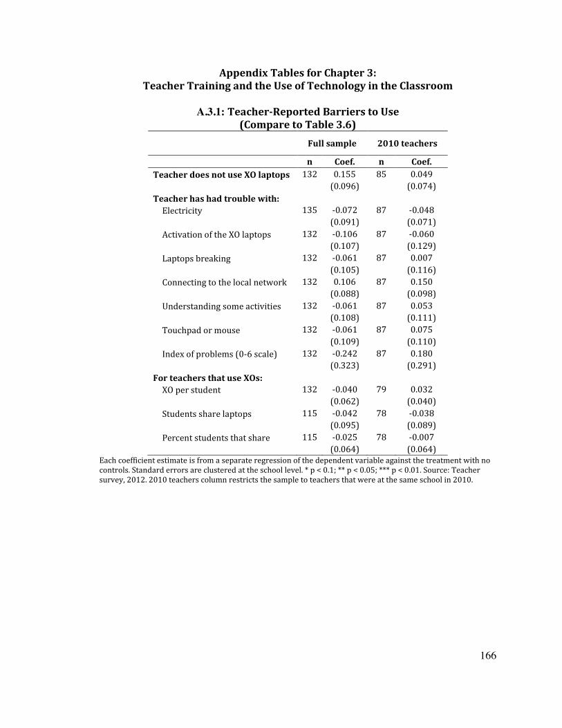
166

Appendix Tables for Chapter 3: Teacher Training and the Use of Technology in the Classroom

A.3.1: Teacher-Reported Barriers to Use

(Compare to Table 3.6)

Full sample 2010 teachers

n Coef. n Coef. Teacher does not use XO laptops 132 0.155 85 0.049 (0.096) (0.074) Teacher has had trouble with:

Electricity 135 -0.072 87 -0.048 (0.091) (0.071)

Activation of the XO laptops 132 -0.106 87 -0.060 (0.107) (0.129)

Laptops breaking 132 -0.061 87 0.007 (0.105) (0.116)

Connecting to the local network 132 0.106 87 0.150 (0.088) (0.098)

Understanding some activities 132 -0.061 87 0.053 (0.108) (0.111)

Touchpad or mouse 132 -0.061 87 0.075 (0.109) (0.110)

Index of problems (0-6 scale) 132 -0.242 87 0.180 (0.323) (0.291)

For teachers that use XOs: XO per student 132 -0.040 79 0.032

(0.062) (0.040) Students share laptops 115 -0.042 78 -0.038

(0.095) (0.089) Percent students that share 115 -0.025 78 -0.007

(0.064) (0.064) Each coefficient estimate is from a separate regression of the dependent variable against the treatment with no controls. Standard errors are clustered at the school level. * p < 0.1; ** p < 0.05; *** p < 0.01. Source: Teacher survey, 2012. 2010 teachers column restricts the sample to teachers that were at the same school in 2010.

167

A.3.2: Teacher Computer Use, XO Knowledge & Opinions

(Compare to Table 3.7) Full sample

2010 teachers

n Coef. n Coef.

Computer use and knowledge Used a PC during the last week 135 0.101 87 0.074 (0.065) (0.083) Accessed the Internet during the last week 135 0.040 87 0.008 (0.081) (0.088) Index of self-assessed computer literacy

(0-4 scale) 135 -0.009 87 0.061

(0.199) (0.240) Knowledge of the XO laptops Index of knowledge on accessing texts on

the XO laptops (0-4 scale) 124 -0.014 82 0.016

(0.180) (0.202) Index of knowledge on the "Calculate"

application (0-4 scale) 121 -0.027 80 -0.108

(0.178) (0.222) Knows how to access data on a USB drive 124 0.075 81 0.093 (0.109) (0.126) Teacher Opinions of the XO Laptops Index of positive opinions of XO (0-8 scale) 131 -0.433 84 -0.595* (0.277) (0.350)

Each coefficient estimate is from a separate regression of the dependent variable against the treatment with no controls. Standard errors are clustered at the school level. * p < 0.1; ** p < 0.05; *** p < 0.01. Source: Teacher survey, 2012. Sample for "2010 teachers" column is restricted to teachers who were in the same school in 2010, the year of the training.

168

A.3.3: Student PC Access, XO Opinions (Compare to Table 3.8)

Full sample 2010

teachers

n Coef. n Coef.

Family has a PC - all 588 0.013 545 0.011 (0.026) (0.028)

2nd graders 207 0.013 188 0.004 (0.047) (0.050)

4th graders 176 0.074** 167 0.078** (0.036) (0.038)

6th graders 205 -0.034 190 -0.039 (0.029) (0.031)

Index of positive opinions of XO (0-5) 587 -0.159 544 -0.228 (0.297) (0.313)

2nd graders 207 0.026 188 -0.118 (0.381) (0.387)

4th graders 175 -0.144 166 -0.108 (0.375) (0.393)

6th graders 205 -0.407 190 -0.484 (0.387) (0.405)

Each coefficient estimate is from a separate regression of the dependent variable against the treatment with no controls. Standard errors are clustered at the school level. * p < 0.1; ** p < 0.05; *** p < 0.01. Source: Student survey, 2012. 2010 teachers column restricts the sample to students whose teachers were at the same school in 2010.

169

A.3.4: Use of the XO Laptops According to Survey Data (Compare to Table 3.9) Full sample 2010 teachers

n Coef. n Coef. Panel A: Usage from Principal Survey

School uses XO laptops 51 -0.005 (0.092) Ratio of functioning XO laptops to student (school level)

49 0.051 (0.146)

Panel B: Usage from Teacher Survey Teacher uses XOs 132 -0.155 85 -0.049 (0.096) (0.074) How many days (0-5) used XO laptop last week by subject areaa

Math 134 -0.112 86 -0.089 (0.235) (0.204) Communication 134 -0.212 86 -0.078 (0.226) (0.192) Science and environment 134 -0.057 86 0.167 (0.239) (0.259) Personal social 134 -0.134 86 0.047 (0.286) (0.324) Art 134 0.030 86 0.191 (0.273) (0.322) Physical education 134 -0.258 86 0.511 (0.528) (0.684) Religious studies 134 -0.296 86 -0.182 (0.338) (0.348) Other 134 0.318 86 1.099 (0.852) (1.214)

Number of different applications usedb 134 -2.243 86 -2.274 (1.509) (1.647) Intensity: Sum of apps * Times usedb 135 -4.848* 87 -5.742* (2.570) (3.082) Percent of application uses among the 10 apps emphasized in training

95 0.079** 68 0.102*** (0.035) (0.035)

Panel C: Usage from Student Survey Child uses XO at school on a typical day 588 -0.040 545 -0.079 (0.092) (0.091) Child shares XO 516 -0.044 484 -0.051 (0.134) (0.140) Child brings XO home occasionally 516 -0.015 484 0.051 (0.124) (0.125) Teacher gives permission to bring XO home 301 0.012 286 0.018

(0.047) (0.050) Parents give permission to bring XO home 301 -0.174* 286 -0.157

(0.095) (0.096) Standard errors, clustered at school level, in parentheses. * p <0.1; ** p <.05; *** p <.01. 2010 teachers column restricts the sample to teachers at the same school in 2010. From OLS regressions except: a Poisson. b Zero-inflated negative binomial.

170

A.3.5: Use of the XO Laptops by Computer Logs

(Compare to Table 3.10)

Full sample 2010 teachers

n Coef. n Coef.

Frequency of use Average number of sessions in last weeka

587 -0.065 374 -0.185 (0.246) (0.268)

2nd grade 205 0.399 108 0.143 (0.306) (0.390) 4th grade 179 -0.244 139 -0.300 (0.293) (0.328) 6th grade 203 -0.369 127 -0.273

(0.342) (0.327) % with 0 sessions 587 0.038 374 0.052 (0.084) (0.095) % with 1 session 587 -0.031 374 -0.014 (0.038) (0.048) % with 2 sessions 587 0.008 374 0.014 (0.029) (0.042) % with 3 sessions 587 -0.011 374 -0.007 (0.020) (0.030) % with 4+ sessions 587 -0.005 374 -0.045

(0.049) (0.054) Intensity of use

Number of application uses in last weeka

587 -0.125 374 -1.090 (1.083) (1.202)

Each coefficient estimate is from a separate regression of the dependent variable against the treatment with no controls. Standard errors, clustered at the school level, are in parentheses. * p < 0.1; ** p < 0.05; *** p < 0.01. OLS regressions except: a Negative binomial regression. Source: Log files from children's computers that record data on the child's most recent four sessions. A session begins when the child turns the computer on and ends when the computer is turned off.

171

A.3.6: Type of Use of the XO Laptops by Computer Logs (Compare to Table 3.11)

Full sample 2010 teachers

n Marginal effects

n Marginal effects

Use of applications emphasized in training Number of uses (10 priority apps) 374 0.206 374 0.742

(1.181) (1.350) Number of uses (15 priority apps) 374 0.136 374 1.879

(1.385) (1.618) % uses that are 10 prioritya 435 0.013 312 0.045 (0.044) (0.048) % uses that are 15 prioritya 435 -0.000 312 0.031 (0.050) (0.062)

By type of application (number of uses) Standard 587 0.199 374 0.864 (0.992) (1.216) Games 587 -0.042 374 0.002 (0.350) (0.350) Music 587 -1.069** 374 -1.436* (0.533) (0.761) Programming 587 0.253 374 0.332 (0.197) (0.208) Other 587 0.540 374 0.984 (0.652) (0.818)

By application material (number of uses) Cognition 587 -0.126 374 -0.087 (0.317) (0.330) Geography 587 0.107 374 0.147 (0.201) (0.304) Reading 587 0.274 374 0.256 (0.640) (0.869) Math 587 0.090 374 0.296* (0.161) (0.154) Measurement 587 -0.025 374 0.014 (0.059) (0.074) Music 587 -1.069** 374 -1.436* (0.533) (0.761) Programming 587 0.178 374 0.251 (0.261) (0.322) Utilitarian 587 -0.341 374 0.187 (0.542) (0.622) Other 587 0.854* 374 1.171* (0.514) (0.670)

Each coefficient estimate is from a separate regression of the dependent variable against the treatment with no controls. Standard errors are in parentheses and are clustered at the school level. * p < 0.1; ** p < 0.05; *** p < 0.01. Source: Log files from children's computers that record data on the child's most recent four sessions. A session begins when the child turns the computer on and ends when the computer is turned off.

172

A.3.7: Effects on Math Scores and Verbal Fluency (Compare to Table 3.12)

Full sample

2010

teachers

n Marginal

effects n

Marginal effects

Math Scores Overall 588 0.080 545 0.039 (0.105) (0.110)

2nd grade 207 -0.154 188 -0.208 (0.191) (0.201) 4th grade 176 0.122 167 0.153 (0.224) (0.235) 6th grade 205 0.177 190 0.074

(0.213) (0.218) 4th and 6th grades 381 0.141 357 0.126

combined (0.148) (0.157) Verbal Fluency Overall 588 0.077 545 0.048 (0.131) (0.140)

2nd grade 207 -0.215 188 -0.227 (0.166) (0.177) 4th grade 176 0.164 167 0.168 (0.201) (0.212) 6th grade 205 0.114 190 0.062

(0.198) (0.213) 4th and 6th grades 381 0.132 290 0.065

combined (0.167) (0.225) Test scores are standardized to have a mean of 0 and a standard deviation of 1 for each grade level. For the overall effects, test scores are standardized for the entire sample. In columns (2) and (3), each estimate is from a separate regression of the test score with no controls. Standard errors, clustered at the school level, are presented in parentheses. * p < 0.1; ** p < 0.05; *** p < 0.01.

173

Appendix Tables for Chapter 4: Teacher’s Helpers

A.4.1: Woodcock Muñoz Language Survey-Revised (WMLS-R) Subtests

Picture vocabulary: measures aspects of oral language, including language development and lexical knowledge. The task requires subjects to identify pictured objects. Verbal analogies: measures the ability to reason using lexical knowledge. Students listen to three words of an analogy and complete it by stating the fourth word. Understanding directions: measures listening, lexical knowledge, and working memory skills. To complete this task, students listen to a series of instructions and demonstrate their comprehension by pointing to a series of objects in a picture. Story recall: measures listening skills, meaningful memory and expressive language. Students are asked to recall increasingly complex stories that they hear in an audio recording.

174

A.4.2: Changes in Balance - Round 2 Sample vs. Attritors

Female Picture Vocabulary

Verbal Analogies

Und. Directions Story Recall Oral

Language

Panel A: DynEd vs. Control Constant 0.481*** 0.349* 0.137 0.237 0.144 0.289 (0.046) (0.191) (0.160) (0.213) (0.150) (0.206) DynEd -0.156* -0.497 -0.434** -0.736** -0.039 -0.580* (0.090) (0.348) (0.186) (0.278) (0.238) (0.302) Round 2 sample 0.040 -0.129 0.060 0.034 -0.012 -0.020 (0.065) (0.165) (0.178) (0.178) (0.134) (0.182) DynEd*Round 2 0.027 0.211 0.226 0.374 -0.068 0.251 (0.108) (0.326) (0.222) (0.276) (0.213) (0.295) n 576 576 576 576 576 576

Panel B: Imagine vs. Control Constant 0.481*** 0.349* 0.137 0.237 0.144 0.289 (0.046) (0.191) (0.159) (0.213) (0.150) (0.206) Imagine Learning 0.096 -0.780*** -0.109 -0.527** -0.413* -0.616** (0.083) (0.224) (0.313) (0.254) (0.226) (0.258) Round 2 sample 0.040 -0.129 0.060 0.034 -0.012 -0.020 (0.065) (0.165) (0.178) (0.178) (0.134) (0.182) Imagine*Round 2 -0.116 0.406* -0.261 0.143 0.123 0.163 (0.097) (0.209) (0.326) (0.236) (0.202) (0.241) 599 599 599 599 599 599

Panel C: DynEd vs. Imagine Constant 0.578*** -0.431*** 0.028 -0.290** -0.269 -0.326** (0.069) (0.118) (0.270) (0.138) (0.169) (0.155) DynEd -0.253** 0.283 -0.325 -0.209 0.374 0.035 (0.103) (0.313) (0.286) (0.225) (0.250) (0.269) Round 2 sample -0.076 0.276** -0.201 0.178 0.110 0.143 (0.071) (0.129) (0.273) (0.155) (0.151) (0.158) DynEd*Round 2 0.143 -0.195 0.487 0.231 -0.191 0.089 (0.111) (0.309) (0.303) (0.262) (0.224) (0.281) n 557 557 557 557 557 557

Standard errors, clustered at the school level, are in parentheses. * p < 0.1; ** p < 0.05; *** p < 0.01.

175

A.4.3: Changes in Balance - Round 3 Sample vs. Attritors

Female Picture Vocabulary

Verbal Analogies

Und. Directions Story Recall Oral

Language

Panel A: DynEd vs. Control Constant 0.460*** 0.131 0.008 -0.029 -0.056 0.028 (0.046) (0.137) (0.137) (0.134) (0.160) (0.134) DynEd -0.108 -0.316 -0.170 -0.361 0.065 -0.285 (0.068) (0.219) (0.188) (0.231) (0.245) (0.234) Round 3 sample 0.076 0.180 0.255* 0.431*** 0.282** 0.365*** (0.057) (0.127) (0.146) (0.109) (0.106) (0.115) DynEd*Round 3 -0.032 -0.023 -0.095 -0.075 -0.242 -0.122 (0.090) (0.233) (0.194) (0.232) (0.215) (0.238) n 576 576 576 576 576 576

Panel B: Imagine vs. Control Constant 0.460*** 0.131 0.008 -0.029 -0.056 0.028 (0.046) (0.137) (0.137) (0.134) (0.160) (0.134) Imagine Learning 0.020 -0.435** -0.305* -0.328* -0.379 -0.462** (0.062) (0.164) (0.172) (0.188) (0.323) (0.209) Round 3 sample 0.076 0.180 0.255* 0.431*** 0.282** 0.365*** (0.057) (0.127) (0.146) (0.109) (0.106) (0.115) Imagine*Round 3 -0.024 -0.016 -0.017 -0.096 0.117 -0.013 (0.081) (0.191) (0.184) (0.200) (0.306) (0.215) 599 599 599 599 599 599

Panel C: DynEd vs. Imagine Constant 0.480*** -0.304*** -0.297*** -0.357*** -0.435 -0.434*** (0.041) (0.091) (0.104) (0.132) (0.281) (0.160) DynEd -0.128* 0.120 0.135 -0.033 0.444 0.177 (0.064) (0.194) (0.165) (0.229) (0.336) (0.250) Round 3 sample 0.052 0.164 0.238** 0.335* 0.399 0.352* (0.057) (0.142) (0.111) (0.168) (0.287) (0.181) DynEd*Round 3 -0.007 -0.006 -0.078 0.020 -0.359 -0.109 (0.090) (0.241) (0.169) (0.265) (0.343) (0.276) 557 557 557 557 557 557

Standard errors, clustered at the school level, are in parentheses. * p < 0.1; ** p < 0.05; *** p < 0.01.