ESD.86Markov Processes and their

Application to Queueing

Richard C. LarsonMarch 5, 2007

Photo courtesy of Johnathan Boeke. http://www.flickr.com/photos/boeke/134030512/

Outline

Spatial Poisson Processes, one more timeIntroduction to Queueing SystemsLittle’s LawMarkov Processes

http://zappa.nku.edu/~longa/geomed/modules/ss1/lec/poisson.gif

SpatialPoissonProcesses

Courtesy of Andy Long. Used with permission.

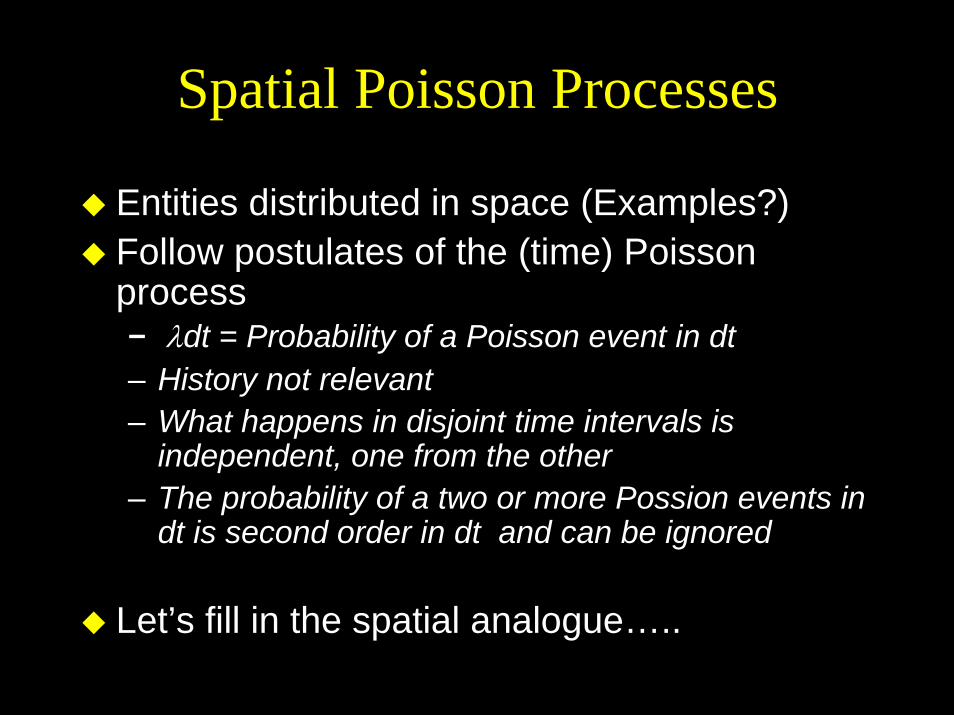
Spatial Poisson Processes

Entities distributed in space (Examples?)Follow postulates of the (time) Poisson process– λdt = Probability of a Poisson event in dt – History not relevant– What happens in disjoint time intervals is

independent, one from the other– The probability of a two or more Possion events in

dt is second order in dt and can be ignored

Let’s fill in the spatial analogue…..

S

Set S has area A(S).Poisson intensity is γPoisson entities/(unit area).

X(S) is a random variable X(S) = number of Poisson

entities in S

P{X(S) = k} = (γA(S))k

k!e−γA (S ), k = 0,1,2,...

Nearest Neighbors: Euclidean

Define D2= distance from a random pointto nearest Poisson entity

Want to derive fD2(r).

r

Random Point

Happiness:FD2

(r) ≡ P{D2 ≤ r} =1− P{D2 > r}

FD2(r) =1−Prob{no Poisson entities in circle of radius r}

FD2(r) =1− e−γπr 2

r ≥ 0

fD2(r) = d

drFD2

(r) = 2rγπe−γπr 2

r ≥ 0

Rayleigh pdf with parameter 2γπ

Nearest Neighbors: Euclidean

Define D2= distance from a random pointto nearest Poisson entity

Want to derive fD2(r).

r

Random Point

fD2(r) = d

drFD2

(r) = 2rγπe−γπr 2

r ≥ 0

Rayleigh pdf with parameter 2γπ

E[D2] = (1/2) 1γ

"Square Root Law"

σD2

2 = (2 −π /2) 12πγ

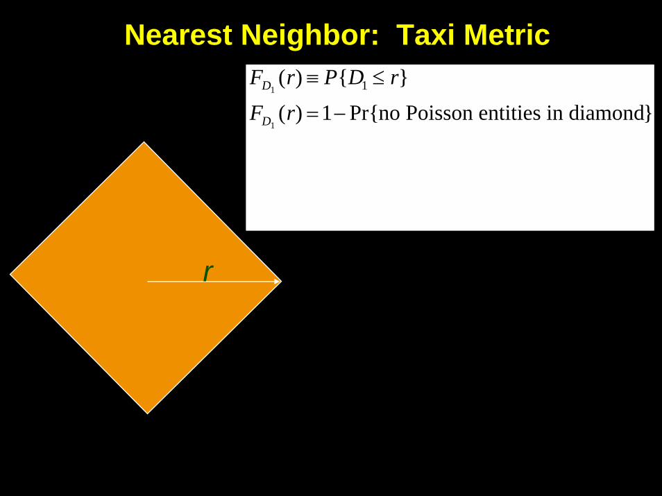
Nearest Neighbor: Taxi Metric

r

FD1(r) ≡ P{D1 ≤ r}

FD1(r) =1−Pr{no Poisson entities in diamond}

FD1(r) =1− e−γ 2r 2

fD1(r) = d

drFD1

(r) = 4rγe−2γr 2

How Might you Derive the PDF fo the kth Nearest Neighbor?

Blackboard exercise!

To Queue or Not to Queue,That May be a Question!

Queue of Waiting Customers

Queueing System

Arriving Customers

Departing Customers

Service Facility

Figure by MIT OCW.

Finite or Infinite?

Finite or Infinite?

Queue Discipline:How queuersAre selected for service

Servers:Statistical Clones?

Source: Larson and Odoni, Urban Operations Research

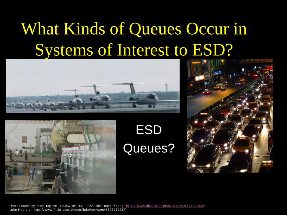
What Kinds of Queues Occur in Systems of Interest to ESD?

ESD Queues?

Photos courtesy, from top left, clockwise: U.S. FAA: Flickr user “*keng” http://www.flickr.com/photos/kengz/67187556/; Luke Hoersten http://www.flickr.com/photos/lukehoersten/532375235/)

Little’s Law for Queues

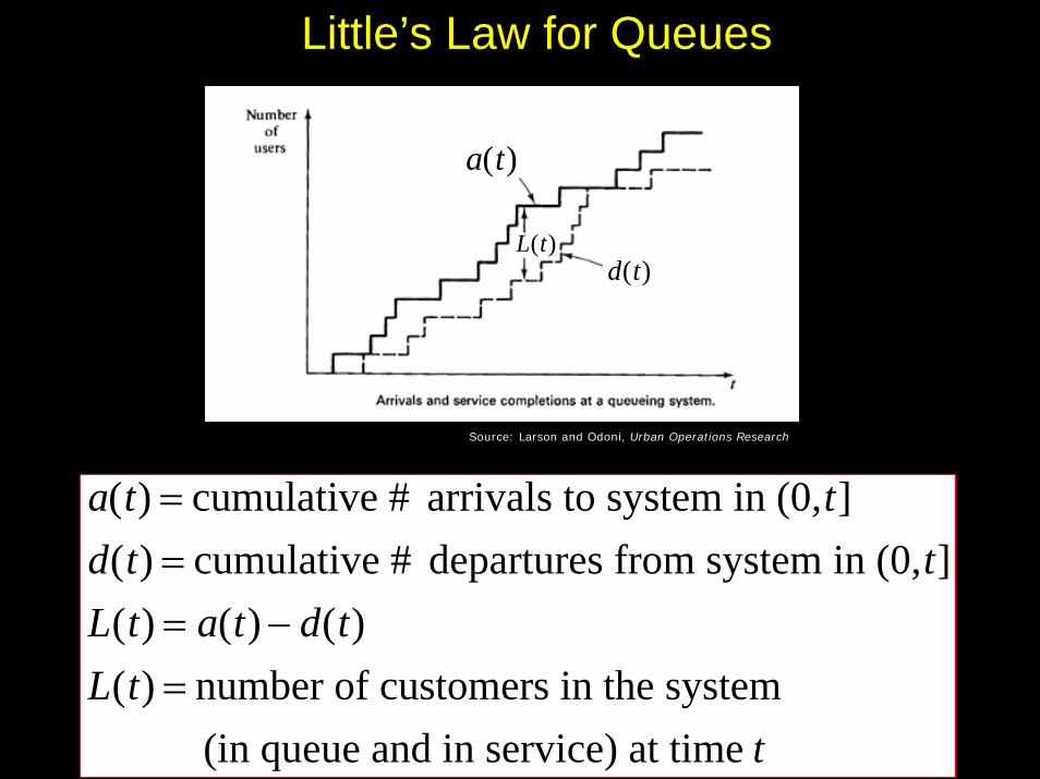
a(t) = cumulative # arrivals to system in (0,t]d(t) = cumulative # departures from system in (0,t]L(t) = a(t) − d(t)L(t) = number of customers in the system (in queue and in service) at time t

d(t)

a(t)

L(t)

Source: Larson and Odoni, Urban Operations Research

Little’s Law for Queues

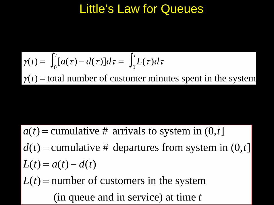
a(t) = cumulative # arrivals to system in (0,t]d(t) = cumulative # departures from system in (0,t]L(t) = a(t) − d(t)L(t) = number of customers in the system (in queue and in service) at time t

γ(t) = [a(τ ) − d(τ)]dτ0

t∫ = L(τ )dτ0

t∫γ(t) = total number of customer minutes spent in the system

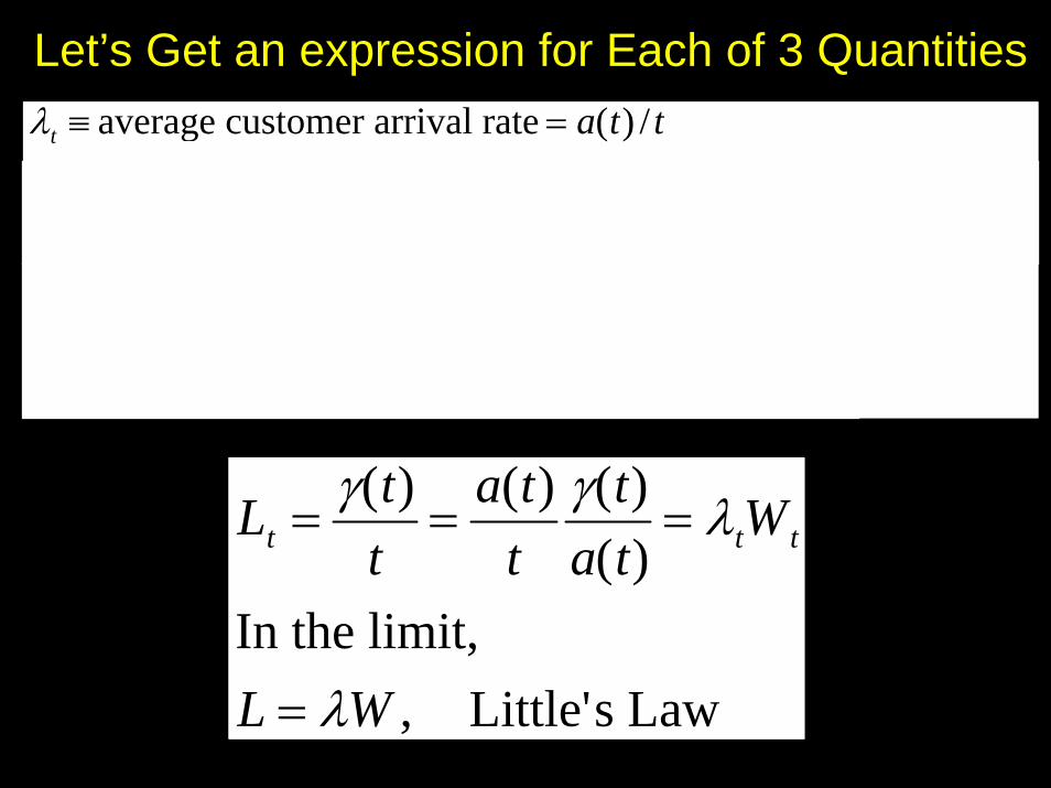
Let’s Get an expression for Each of 3 Quantitiesλt ≡ average customer arrival rate = a(t) / tWt ≡ average time that an arrived customer has spent in the systemWt = γ(t) /a(t)Lt = time average # customers in system during (0,t]

Lt =1t

L(τ )dτ = γ(t) / t0

t∫

Lt =γ(t)

t=

a(t)t

γ(t)a(t)

= λtWt

In the limit,L = λW , Little's Law

Key Issues

L in a time-average. Explainλ is average of arrival rate of customers who actually enter the systemW is average time in system (in queue and in service) for actual customers who enter the system

L = λW

More Issues

Little’s Law is general. It does not depend on– Arrival process– Service process– # servers– Queue discipline– Renewal assumptions, etc.

It just requires that the 3 limits exist.

L = λW

Still More Issues

What about balking? Reneging? Finite capacity?Do we need iid service times? Iid inter-arrival times?Do we need each busy period to behave statistically identically?Look at role of γ(t). Can change queue statistics by changing queue discipline.

L = λW

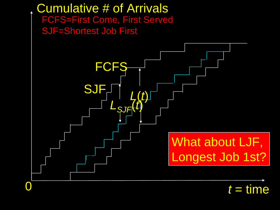
t = time

Cumulative # of Arrivals

0

L(t)

FCFS

SJFLSJF(t)

FCFS=First Come, First ServedSJF=Shortest Job First

What about LJF,Longest Job 1st?

“System” is General

Our results apply to entire queue system, queue plus service facilityBut they could apply to queue only!

Or to service facility only!

L = λW

S.F. Lq = λWq

LSF = λWSF = λ /μ1/μ = mean service time

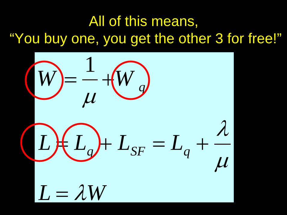
All of this means,“You buy one, you get the other 3 for free!”

W =1μ+W q

L = Lq + LSF = Lq +λμ

L = λW

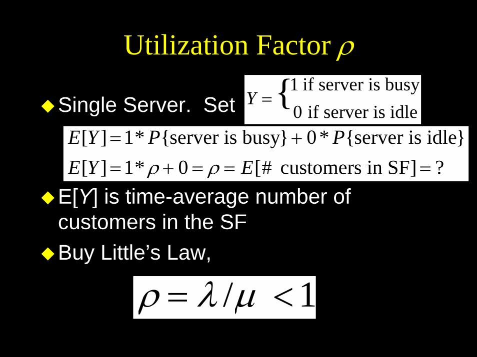
Utilization Factor ρ

Single Server. Set

E[Y] is time-average number of customers in the SFBuy Little’s Law,

Y ={1 if server is busy0 if server is idle

E[Y] =1* P{server is busy}+ 0 * P{server is idle}E[Y] =1* ρ + 0 = ρ = E[# customers in SF] = ?

ρ = λ /μ <1

Utilization Factor ρ

Similar logic for N identical parallel servers gives

Here, λ/μ corresponds to the time-average number of servers busy

ρ = ( λN

) 1μ=

λNμ

<1

Markov Queues

Markov here means, “No Memory”

Source: Larson and Odoni, Urban Operations Research

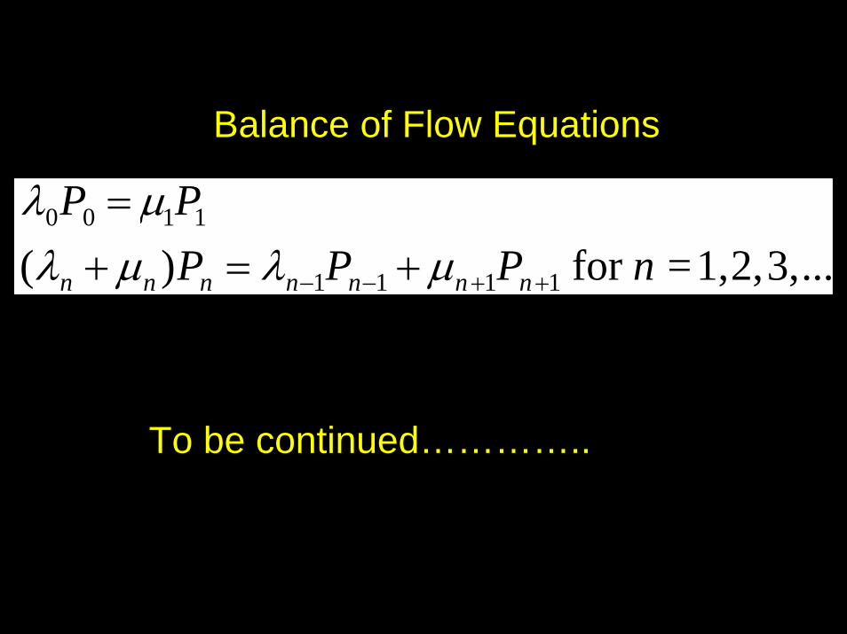
Balance of Flow Equations

To be continued…………..

λ0P0 = μ1P1

(λn + μn )Pn = λn−1Pn−1 + μn+1Pn+1 for n =1,2,3,...