DISCRETE AND CONTINUOUS doi:10.3934/dcdsb.2009.11.1057DYNAMICAL SYSTEMS SERIES BVolume 11, Number 4, June 2009 pp. 1057–1070

ERROR ANALYSIS OF STABILIZED SEMI-IMPLICIT METHOD

OF ALLEN-CAHN EQUATION

Xiaofeng Yang

Department of Mathematics, University of North Carolina at Chapel HillChapel Hill, NC 27599, USA

(Communicated by Jie Shen)

Abstract. We consider in this paper the stabilized semi-implicit (in time)scheme and the splitting scheme for the Allen-Cahn equation φt − ∆φ +ε−2f(φ) = 0 arising from phase transitions in material science. For the sta-

bilized first-order scheme, we show that it is unconditionally stable and theerror bound depends on ε−1 in some lower polynomial order using the spec-trum estimate of [2, 10, 11]. In addition, the first- and second-order operatorsplitting schemes are proposed and the accuracy are tested and compared withthe semi-implicit schemes numerically.

1. Introduction. In this paper, we consider numerical schemes in the semi-discreteform (in time) to solve the Allen-Cahn equation

φt − ∆φ+1

ε2f(φ) = 0, (x, t) ∈ Ω × (0, T ),

∂φ

∂n

|∂Ω = 0, φ(t0) = φ0.

(1)

where Ω ⊂ ℜN , N = 1, 2, 3 is a bounded domain with C1,1 boundary ∂Ω or a convexpolygonal domain, n is the outward normal, f(φ) = F ′(φ) and F (φ) = 1

4 (φ2−1)2, adouble equal well potential which takes the global minimum value at φ = ±1. Theequation (1) was originally introduced by Allen-Cahn [1] to describe the motion ofanti-phase boundaries in crystalline solids. φ represents the concentration of one ofthe two metallic components of the alloy and the parameter ε represents the interfa-cial length, which is extremely small compared to the characteristic dimensions onthe laboratory scale. The homogenous Neumann boundary condition implies thatno mass loss occurs across the boundary walls. The Allen-Cahn equation can also beviewed as a gradient flow with Liapunov energy functional

∫

Ω 1

2 |∇φ|2 + 1

ε2F (φ)dx.As ε→ 0, the zero level set of φ approaches to a surface which evolves according tothe geometric law of V = κ, where V and κ are the normal velocity and the meancurvature of the surface respectively [1]. Recently, the Allen-Cahn equation hasbeen widely applied to many complicated moving interface problems, for example,vesicle membranes, the nucleation of solids and the mixture of two incompressiblefluids, etc. (cf.[4, 5, 6, 9, 18, 19, 20]).

2000 Mathematics Subject Classification. Primary: 65M12, 76T99; Secondary: 65M70.Key words and phrases. Allen-Cahn equation, semi-implicit methods, error analysis.The author is supported by AFOSR FA9550-06-1-0063.

1057

1058 XIAOFENG YANG

The main difficulty when one wants to design the numerical scheme of (1) is thatthe nonlinear penalty term f(φ) will yield a severe stability limitation on the timestep when a usual implicit or explicit scheme is adopted (on f(φ)). In particular,the time step constraint relates to o(ε2) in both ways. It is also embarrassing if oneattempts to obtain error bounds using the straight forward perturbation argument.The error bounds will depend on the factor of O(e1/ε) which tends to infinity whenε→ 0. In [7], the spectrum argument [2, 10, 11] was applied to derive the rigorouserror bounds for the implicit scheme (for f(φ)). The optimal error bounds obtainedare in terms of some lower polynomial order of ε−1. The same spectral argument isalso applied to derive a similar a posteriori error estimate in [8]. For the overview onthe topic of convergence analysis of the numerical schemes, we refer to [7, 12, 13, 14].

In this article, we consider the first- and second-order (in time) stabilized semi-implicit schemes. The nonlinear term f(φ) is treated explicitly in order to avoiditerations and speed up the numerical computation. An extra stabilizing term isadded to alleviate the stability constraint while maintaining accuracy and simplicity.We derive a priori energy estimates which show that the first-order scheme is stableif its solution in some norm remains to be bounded as δt → 0. Furthermore, usingthe same spectral argument, the optimal error estimate is also proved for the first-order stabilized semi-implicit numerical scheme.

We also consider, as an alternative, the first-order sequential splitting methodand the second-order Strang splitting method [15]. The splitting method is uncon-ditionally stable but suffers from a splitting error. For the examples we tested, itis found that the first-order sequential splitting method is more accurate than thefirst-order semi-implicit scheme when some larger time steps are used. However, forthe second-order scheme, the accuracy is reversed.

The paper is organized as follows. In section 2, we describe the stabilized first- andsecond-order semi-implicit schemes as well as the first- and second-order operatorsplitting schemes. We then establish the a priori energy estimates for the first-ordersemi-implicit scheme and derive the optimal error estimates using the spectrumargument in section 3. Numerical tests of the semi-implicit schemes and the splittingschemes for a classical benchmark problem and some concluding remarks are givenfinally in section 4.

2. Time discretization of the Allen-Cahn equation. In this section, we de-scribe two classes of efficient time discretization schemes. A good feature sharedby these schemes is that only Poisson-type equations have to be solved at eachtime step. Hence they are particularly suitable for spatial discretizations with fastPoisson solvers.

2.1. The stabilized semi-implicit method. The first-order stabilizedsemi-implicit scheme is

φm − φm−1

k− ∆φm +

1

ε2(f(φm−1) + s(φm − φm−1)) = 0,

∂φm

∂n

∣

∣

∂Ω= 0.

(2)

ERROR ANALYSIS OF ALLEN-CAHN EQUATION 1059

The second-order stabilized semi-implicit scheme is

3φm+1 − 4φm + φm−1

2δt− ∆φm+1 +

1

ε2

(

2f(φm) − f(φm−1)

+ s(φm+1 − 2φm + φm−1))

= 0,

∂φm+1

∂n

∣

∣

∂Ω= 0.

(3)

Remark 2.1. The schemes (2) and (3) first appeared in [8, 9, 18, 19]. They are quitestable and robust even in the phase-field model where the Allen-Cahn equation iscoupled with the Navier-Stokes equations. It is clear that the explicit (and even fullyimplicit [7]) treatment of the nonlinear term f(φ) usually leads to a restriction onthe time step δt when ε << 1. Therefore, the extra dissipative term s

ε2 (φm−φm−1)

(order of sδtε2 ) in (2) and sε2 (φm+1 − 2φm+φm−1) (order of sδt

2

ε2 ) in (3) are added toimprove the stability while preserving the simplicity. The similar technique of thestabilizer also appeared in [17]. The parameter s is proportional to the amount ofartificial dissipation added in the numerical scheme. Larger s will lead to a morestable but less accurate scheme. Numerical results indicate that s = 1 [9] in theCartesian coordinates and s = 5 [18] in the cylindrical coordinates provide a goodbalance between accuracy and stability.

2.2. The operator splitting method. Consider a general evolution equation like

∂u

∂t= g(u) = Au+Bu, (4)

where g(u) is a nonlinear operator. The choices of A and B are arbitrary becauseA and B do not need commute. The first-order splitting method for (4) [15] is

∂u

∂t= Au, u(tm) = um, tm ≤ t ≤ tm+1,

∂u

∂t= Bu, u(tm) = um+1, tm ≤ t ≤ tm+1.

(5)

In particular, for the Allen-Cahn equation (1), the first-order splitting method is

∂φ

∂t+

1

ε2f(φ) = 0, φ(tm) = φm, tm ≤ t ≤ tm+1, (6)

∂φ

∂t− ∆φ = 0, φ(tm) = φm+1, tm ≤ t ≤ tm+1. (7)

The second-order splitting method is

∂φ

∂t+

1

ε2f(φ) = 0, φ(tm) = φm, tm ≤ t ≤ tm+ 1

2, (8)

∂φ

∂t− ∆φ = 0, φ(tm) = φm+1, tm ≤ t ≤ tm+1, (9)

∂φ

∂t+

1

ε2f(φ) = 0, φ(tm+ 1

2) = φm+1, tm+ 1

2≤ t ≤ tm+1. (10)

For (6), (8) and (10), the exact solutions are

φm+1 =φm

√

φ2m + (1 − φ2

m)e−2

ε2 (tm+1−tm), (11)

φm+1/2 =φm

√

φ2m + (1 − φ2

m)e−2

ε2 (tm+1/2−tm), (12)

1060 XIAOFENG YANG

and

φm+1 =φm+1

√

φ2m+1 + (1 − φ2

m+1)e− 2

ε2 (tm+1−tm+1/2), (13)

respectively. For (7) and (9), we use the second-order semi-implicit scheme:

φm+1 − φm+1

δt=

1

2(∆φm+1 + ∆φm+1). (14)

Remark 2.2. The first- and second-order splitting schemes are unconditionally stablebecause of the unconditional stability of each sub-step.

3. Energy estimates and error analysis. In this section, a priori energy esti-mates are established for the Allen-Cahn equation (1) and the first-order stabilizednumerical scheme (2). The optimal error estimates are also derived thereafter.

3.1. Energy estimates for PDE. We now introduce some notations. LetW s,p(Ω)and W

s,p0 (Ω) denote the usual Sobolev spaces equipped with the norm ‖ · ‖s,p for

0 ≤ s <∞, 0 ≤ p ≤ ∞. In particular, we denote the Hilbert spaces W s,2(Ω) by Hs

(s = 0,±1, · · · ) with norm ‖ · ‖s and semi norm | · |s. The norm and inner productof L2(Ω) = H0(Ω) are denoted by ‖ · ‖0 and (·, ·) respectively.

Let k = δt be the time step and set tn = nk for 0 ≤ n ≤ N = [Tk ]. For anyfunction which is continuous in time, u(t), we denote un = u(tn) and define the

difference operator dt by dtun = un−un−1

k . We denote by c a generic constant thatis independent of δt and ε but possibly depends on the data and the solution. Weshall use A . B to say that there is a generic constant that A ≤ cB.

We assume that the initial value of φ0 in (1) satisfies ‖φ0‖L∞ ≤ 1 so that thefollowing maximum principle for the solution of (1) holds (cf. [1, 2, 3, 7, 9]):

Lemma 3.1. If φ0 ∈ [−1, 1] a.e. in Ω, then φ ∈ [−1, 1] a.e in Ω × [0, T ].

In order to trace the dependence of the solution on ε, we also assume φ0 ∈H1(Ω) ∩H2(Ω) and satisfies the following assumptions:There exist nonnegative constants σ1, σ2, σ3 such that

Γε(φ0) =1

2‖∇φ0‖

20 +

1

ε2

∫

Ω

F (φ0)dx . ε−2σ1 . (H1)

‖∆φ0 − ε−2f(φ0)‖0 . ε−σ2 . (H2)

limx→0+‖∇φt(x)‖0 . ε−σ3 . (H3)

Lemma 3.2. ∀t ∈ [0, T ], the solution of (1) satisfies the following energy estimates,

1

2‖∇φ(t)‖2

0 +1

ε2

∫

Ω

|F (φ(t))|dx +

∫ t

0

‖φt‖20dτ = Γε(φ0), (15)

∫ t

0

‖∆φ‖20dτ . ε−2σ1−2, (16)

‖φt(t)‖20 + ‖∆φ(t)‖2

0 +

∫ t

0

‖∇φt(τ)‖20dτ . ε2min(−σ1−1,−σ2), (17)

∫ t

0

‖φtt(τ)‖2−1dτ . ε2min(−σ1−2,−σ2), (18)

∫ t

0

‖φtt(τ)‖20dτ . ε2min(−σ1−2,−σ3). (19)

ERROR ANALYSIS OF ALLEN-CAHN EQUATION 1061

Proof. Taking the inner product of (1) with φt, we derive

‖φt‖20 +

1

2∂t‖∇φ‖

20 +

1

ε2∂t

∫

Ω

|F (φ)|dx = 0. (20)

After the integration over [0, t], we obtain (15). Taking the inner product of (1)with −∆φ and using the Schwarz inequality and Lemma 3.1, we obtain

‖∆φ‖20 = (φt,∆φ) − ε−2(f(φ),−∆φ)

≤1

2‖φt‖

20 +

1

2‖∆φ‖2

0 − ε−2((3φ2 − 1)∇φ,∇φ)

≤1

2‖φt‖

20 +

1

2‖∆φ‖2

0 + 2ε−2‖∇φ‖20.

(21)

After integrating over [0, t] and using (15), we derive∫ t

0

‖∆φ‖20dτ ≤

∫ t

0

‖φt‖20dτ + 4ε−2

∫ t

0

‖∇φ‖20dτ . ε−2σ1−2. (22)

We differentiate (1) in time to obtain

φtt − ∆φt +1

ε2f ′(φ)φt = 0. (23)

After taking the inner product with φt, we infer

1

2∂t‖φt‖

20 + ‖∇φt‖

20 + ε−2(f ′(φ)φt, φt) = 0. (24)

We then integrate over [0, t] to derive

1

2‖φt‖

20 +

∫ t

0

‖∇φt‖20dτ ≤

1

2‖φt(0)‖2

0 + 2ε−2

∫ t

0

‖φt‖20dτ

. ε−2σ2 + ε−2σ1−2.

(25)

Also from (15), (17) and (21), we derive that

‖∆φ‖20 ≤ ‖φt‖

20 + 4ε−2‖∇φ‖2

0 . ε2min(−σ1−2,−σ2). (26)

From (23) and Lemma 3.1, we obtain

‖φtt‖−1 ≤ ‖∇φt‖0 + ε−2supψ∈H1(Ω)

(f ′(φ)φt, ψ)

‖ψ‖1

. ‖∇φt‖0 + ε−2‖f ′(φ)‖L∞‖φt‖0

. ‖∇φt‖0 + ε−2‖φt‖0.

(27)

After squaring the above inequality and integrating over [0, t], we obtain (18). Fi-nally, taking the inner product of (23) with φtt, we derive

‖φtt‖20 +

1

2∂t‖∇φt‖

20 +

1

ε2(f ′(φ)φt, φtt) = 0. (28)

By Schwarz inequality, the last term of the left hand side can be bounded as

1

ε2(f ′(φ)φt, φtt) ≤

1

2‖φtt‖

20 +

1

2ε4‖f ′(φ)‖L∞‖φt‖

20. (29)

After integrating over [0, t], we obtain (19).

1062 XIAOFENG YANG

3.2. A priori energy estimates for the first-order stabilized scheme. Thanksto the maximum principle, we can modify the nonlinear function f to be

f(x) =

f(x), |x| ≤ 2;

11x− 16, x ≥ 2;

11x+ 16, x ≤ −2;

(30)

without affecting the solution and f ∈ C1(ℜ). The function f is now Lipschitzcontinuous with Lipschitz constant L0. We can also assume ‖f ′(x)‖L∞ ≤ L0. For

convenience, we consider the problem formulated with the substitute f , but omitthe tilde in the notation. The symbol F is still used to be the nonlinear potentialsuch that F ′(x) = f(x). Furthermore, f ′ is also Lipschitz continuous. Hence, wewill use L to represent the Lipschitz constant of f and f ′ for convenience.

We are now in position to establish the following:

Theorem 3.1. When s ≥ 32L, the scheme (2) is stable and the solution satisfies

the following energy estimates:

k

M∑

m=1

‖dtφm‖20 +

k

2

M∑

m=1

k‖dt∇φm‖20 + Γε(φM ) ≤ Γε(φ0).

Proof. First, we rewrite (2) for convenience,

dtφm − ∆φm + ε−2f(φm−1) + skε−2dtφm = 0,

∂φm

∂n

∣

∣

∂Ω= 0.

(31)

Second, we take the inner product of (31) with dtφm, we obtain

‖dtφm‖20 +

1

2dt‖∇φm‖2

0 +k

2‖dt∇φm‖2

0 + skε−2‖dtφm‖20

+ ε−2(f(φm), dtφm) = ε−2(f(φm) − f(φm−1), dtφm).(32)

From the Taylor expansion, we derive

(f(φm), dtφm) =1

k(F (φm) − F (φm−1), 1)

+1

2k(f ′(ξ)(φm − φm−1), φm − φm−1)

≥dt

∫

Ω

|F (φm)|dx−kL

2‖dtφm‖2

0,

(33)

here ξ is a value between φm and φm−1. By the Lipschitz continuity of f , we have

ε−2(f(φm) − f(φm−1), dtφm) ≤ Lε−2k‖dtφm‖20. (34)

After combining the above inequalities together, we obtain

(1 + (s−3

2L)kε−2)‖dtφm‖2

0 +1

2dt‖∇φm‖2

0 +k

2‖dt∇φm‖2

0

+ ε−2dt

∫

Ω

|F (φm)|dx ≤ 0.(35)

Finally, after multiplying by k and taking the summation from m = 0 to M , wecan obtain

ERROR ANALYSIS OF ALLEN-CAHN EQUATION 1063

k

M∑

m=0

(1 + (s−3

2L)kε−2)‖dtφm‖2

0 +1

2‖∇φM‖2

0

+1

2k

M∑

m=0

k‖dt∇φm‖20 + ε−2

∫

Ω

|F (φM )|dx

≤1

2‖∇φ0‖

20 + ε−2

∫

Ω

|F (φ0)|dx = Γε(φ0).

(36)

Remark 3.1. For the explicit scheme, i.e. s = 0, the constraint of the time step

comes from the condition of 1− 32Lkε

−2 ≥ 0, i.e. k ≤ 2ε2

3L . Actually, for the implicit

scheme (s = 0 and replace f(φm−1) by f(φm) in (2)), there still exists the time stepconstraint of k ≤ ε2, the detailed proof is in [7].

In order to obtain the error bounds, we also need the following two energy esti-mates in H2-norm.

Lemma 3.3. If k . ε2, the following energy estimates hold:

k

M∑

m=1

‖∆φm‖20 . ε−2σ1−2, (37)

‖∆φm‖20 + ‖dtφM‖2

0 + k

M∑

m=0

‖∇dtφm‖20 . ε2min(−σ2,−σ1−1). (38)

Proof. We take the inner product of (31) with −∆φm and use the Schwarz inequal-ity, we obtain

‖∆φm‖20 =(dtφm,∆φm) − ε−2(f(φm−1),−∆φm) + skε−2(dtφm,∆φm)

≤1

2‖∆φm‖2

0 + (1 + s2k2ε−4)‖dtφm‖20

+1

2Lε−2(‖∇φm‖2

0 + ‖∇φm−1‖20).

(39)

After multiplying by k and taking the summation from m = 1 to M , we derive

k

M∑

m=1

‖∆φm‖20 ≤2Lε−2k

M∑

m=1

‖∇φm‖20 + Lε−2k‖∇φ0‖

20

+ 2(1 + s2k2ε−4)

M∑

m=1

k‖dtφm‖20.

(40)

Let Ck,ε = kε−2 ≤ 1, from Theorem 3.1 and (H1), we obtain

k

M∑

m=1

‖∆φm‖20 ≤ 2Γε(φ0)(1 + LCk,ε + s2C2

k,ε + 2LTε−2)

. ε−2σ1−2.

(41)

We apply dt to both sides of (31) and do the inner product with dtφm, we have

(1 + skε−2)(1

2dt‖dtφm‖2

0 +k

2‖d2tφm‖2

0) + ‖∇dtφm‖20

+ ε−2(dtf(φm−1), dtφm) = 0.(42)

1064 XIAOFENG YANG

From the Lipschitz continuity of f and Schwarz inequality,

ε−2(dtf(φm−1), dtφm) ≤Lε−2

2(‖dtφm‖2

0 + ‖dtφm−1‖20). (43)

After multiplying k and taking the summation from m = 2 to M , we obtain

‖dtφM‖20 + k

M∑

m=2

k‖d2tφm‖2

0 + k

M∑

m=2

‖∇dtφm‖20

.‖dtφ1‖20 + ε−2Γε(φ0).

(44)

From (39), we have

‖∆φm‖20 ≤ 2(1 + s2k2ε−4)‖dtφm‖2

0 + Lε−2(‖∇φm‖20 + ‖∇φm−1‖

20)

. ‖dtφ1‖20 + ε−2Γε(φ0).

(45)

Finally, taking the inner product with dtφ1 with (31) when m = 1, we obtain

‖dtφ1‖20 + k‖∇dtφ1‖

20 ≤ ‖∆φ0 − ε−2f(φ0)‖

20 . ε−2σ2 , (46)

then we complete the proof.

Remark 3.2. This time step constraint condition k . ε2 is inevitable for the energyestimates in higher norm and the error estimates in the following subsection.

3.3. Error analysis for the first-order scheme. In this subsection, we give theerror bounds for the first-order scheme (2). In order to avoid the dependence of e1/ε

caused by the Gronwall’s lemma, we have to use the spectral estimate [2, 10, 11].

Lemma 3.4 (Spectral estimate). Define

LAC = −∆ + f′(φ)I, (47)

where I is the identity operator and φ is the solution of the Allen-Cahn equation.There exists a positive ε-independent constant C0 such that the principle eigenvalueof the linearized Allen-Cahn operator LAC satisfies for ε ≥ 0

λAC ≡ infψ∈H1,ψ 6=0

‖∇ψ‖2 + 1ε2 (f′(φ)ψ, ψ)

‖ψ‖2≥ −C0. (48)

From the maximum principle, the spectral estimate is still suitable for the currentmodified function f in (30). Hence we have the error estimate of the first-orderscheme (31) as follows.

Theorem 3.2. Under the assumptions (H1 − H3) and suppose

k . min(ε2, εα1 , εα2), (49)

the solution of (2) satisfies the following error estimates

‖φ(tm) − φm‖0 . kεmin(−σ1−2,−σ3), (50)

(

k

M∑

m=0

‖∇(φ(tm) − φm)‖20

)12 . kεmin(−σ1−3,−σ3−1). (51)

Proof. Let em = φ(tm) − φm and subtract (31) from (1), we can obtain

dtem − ∆em + ε−2(f(φ(tm)) − f(φm−1)) − skε−2dtφm = Rm, (52)

where

Rm = −1

k

∫ tm

tm−1

(s− tm−1)φtt(s)ds. (53)

ERROR ANALYSIS OF ALLEN-CAHN EQUATION 1065

From (19), we have

k

M∑

m=0

‖Rm‖20 ≤

1

k

∫ tm

tm−1

‖φtt(s)‖20ds

M∑

m=0

∫ tm

tm−1

(s− tm)2ds

. k2ε2min(−σ1−2,−σ3).

(54)

We take the inner product of (52) with em, we obtain

1

2dt‖em‖

20 +

k

2‖dtem‖2

0 + ‖∇em‖20 +

1

ε2(f(φ(tm)) − f(φm), em)

+1

ε2(f(φm) − f(φm−1), em) − skε−2(dtφm, em)

=(Rm, em).

(55)

Notice that f(a) − f(b) =∫ a−b

0f ′(a− ξ)dξ, we derive

(f(φ(tm)) − f(φm), em) =(

∫ em

0

f ′(φ(tm) − ξ)dξ, em)

=(

∫ em

0

(f ′(φ(tm) − ξ) − f ′(φ(tm)))dξ, em)

+ (

∫ em

0

f ′(φ(tm))dξ, em)

≥−L

2ε2‖em‖

3L3 + (f ′(φ(tm))em, em).

(56)

By the Schwarz inequality, we obtain

skε−2(dtφm, em) ≤1

2k2ε−4‖dtφm‖2

0 +1

2s2‖em‖

20,

−1

ε2(f(φm) − f(φm−1), em) ≤

1

2k2ε−4‖dtφm‖2

0 +1

2L2‖em‖

20,

(Rm, em) ≤1

2‖Rm‖

20 +

1

2‖em‖

20.

(57)

From the Lemma 3.4, we obtain

1

2dt‖em‖

20 +

k

2‖dtem‖2

0 ≤(C0 +1 + L2 + s2

2)‖em‖

20

+ k2ε−4‖dtφm‖20 +

1

2‖Rm‖

20 +

L

2ε2‖em‖

3L3 .

(58)

After multiplying 2k, taking the summation from m = 0 to M and using (54), weobtain

‖eM‖20 + k

M∑

m=0

k‖dtem‖20 ≤(1 + 2C0 + L2 + s2)k

M∑

m=0

‖em‖20

+ k2ε−2(σ1+2) + k2ε2min(−σ1−2,−σ3)

+ Lε−2‖em‖3L3.

(59)

To handle the L3 space, we apply a shift in the sub-index to obtain

‖em‖3L3 ≤ C(‖em−1‖

3L3 + k3‖dtem‖3

L3). (60)

1066 XIAOFENG YANG

We interpolate L3 between L2 and H2 and use (17) and (38) to get

‖em‖3L3 . (‖∆em‖

N4

0 ‖em‖3−N

4

0 + ‖em‖30)

. εN4

min(−σ1−1,−σ2)‖em‖3−N

4

0 .(61)

Similarly, the second term of (60) can be bounded by

k3‖dtem‖3L3 . k3(‖∆dtem‖

N4

0 ‖dtem‖3−N

4

0 + ‖dtem‖30)

. k3‖dtem‖3−N

4

0 (‖∆dtem‖N4

0 + ‖dtem‖N4

0 )

. k3−N4 ε

N4

min(−σ1−1,−σ2)‖dtem‖3−N

4

0

. k3−N4 εmin(−σ1−1,−σ2)‖dtem‖

20.

(62)

We multiply kε−2 to (60) and sum it up over m from 0 to ℓ, we obtain

kε−2ℓ

∑

m=0

‖em‖3L3 .ε

N4

min(−σ1−1,−σ2)−2k

ℓ∑

m=0

‖em‖3−N

4

0

+ k3−N4 εmin(−σ1−1,−σ2)−2k

ℓ∑

m=0

‖dtem‖20.

(63)

The second term can be absorbed by the corresponding term on the left hand sideof (59) if

k . εα1 ,with α1 =4max(σ1 + 1, σ2) + 8

8 −N. (64)

Then (59) turns to

‖eM‖20 + k

M∑

m=0

k‖dtem‖20 .k

M∑

m=0

‖em‖20 + k2ε2min(−σ1−2,−σ3)

+ εN4

min(−σ1−1,−σ2)−2k

M∑

m=0

‖em‖3−N

4

0 .

(65)

Finally, we do the inductive argument as the following: Suppose for 0 ≤ m ≤ ℓ, wehave the following inequality

‖em‖20 + k

ℓ∑

m=1

k‖dtem‖20 . k2ε2min(−σ1−2,−σ3). (66)

Notice that the exponent of the last term in (65) is bigger than 2, hence, we canrecover (66) by using the discrete Gronwall’s inequality, provided k satisfies

εN4

min(−σ2,−σ1−1)−2[k2ε2min(−σ2−2,−σ3)]32−N

8

.k2ε2min(−σ2−2,−σ3).(67)

This provide another constraint of k . εα2 with

α2 = max(σ1 + 2, σ3) +Nmax(σ1 + 1, σ2) + 8

4 −N, (68)

then we have (50).

ERROR ANALYSIS OF ALLEN-CAHN EQUATION 1067

To obtain the estimate of H1 norm, in (55), we use Schwarz inequality as follows.

ε−2(f(φ(tm)) − f(φm), em) . ε−2‖em‖20,

kε−2(f(φm) − f(φm−1), em) . k2ε−2‖dtφm‖20 + ε−2‖em‖2

0,

skε−2(dtφm, em) . k2ε−2‖dtφm‖20 + ε−2‖em‖2

0.

(69)

Then we have1

2dt‖em‖

20 + ‖∇em‖

20 . k2ε−2‖dtφm‖2

0 + ε−2‖em‖20 + ‖Rm‖

20. (70)

After multiplying k and taking the summation fromm = 0 toM , we obtain (51).

3.4. Second-order scheme. Numerical results reported in section 4 clearly in-dicate that the second-order scheme is more accurate than the first-order schemeunder the same time step. However, the rigorous proof of the stability and theaccuracy are still elusive.

4. Numerical results and discussions. In this section, we compare the accu-racy between the splitting schemes and the stabilized semi-implicit schemes for theclassical benchmark problem in [3]. The problem is described as follows. At theinitial state, there is a circular interface boundary with a radius of R0 = 100 in therectangular domain of [0, 256] × [0, 256]. Such a circular interface is unstable andthe driving force will shrink and eventually disappear. It is easily shown, in thelimit that the radius of the circle is much larger than the interfacial thickness, thevelocity of the moving interface V is given by

V =dR

dt= −

1

R, (71)

where R is the radius of the circle at a given time t. After taking the integration,we obtain

R2 = R20 − 2t. (72)

We use Spectral-Galerkin method to handle the spatial discretization [16]. In orderto omit the error induced from the space, 513×513 Legendre-Gauss-Lobatoo pointsare used. After we map the domain to [−1, 1] × [−1, 1], we obtain the followingphase equation

φt − γ(∆φ−f(φ)

ε2) = 0, (73)

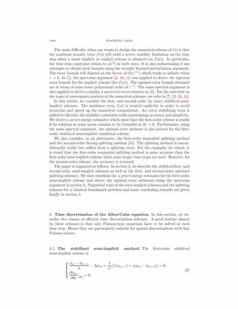
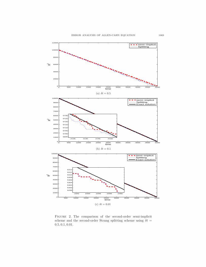
where γ = 6.10351×10−5 and ε = 0.0078. The square of the radius as a function oftime obtained from the splitting scheme and the semi-implicit scheme are shown inFigure 1 and Figure 2. Three time steps δt = 0.1, 0.01, 0.001 and δt = 0.5, 0.1, 0.01are used to test the accuracy of the first- and second-order schemes, respectively.For the first-order scheme, the splitting method shows the competence especiallywhen time steps are larger. When time step is smaller, both of these schemes arevery accurate, for example, Figure 1 (c) and Figure 2 (b),(c). However, the semi-implicit method shows its advantage for the second-order scheme at larger timesteps, for example, Figure 2 (a).

To conclude, we show in this paper that the first-order semi-implicit stabilizedscheme is unconditionally stable and derive the optimal error estimates with poly-nomial growth in ε−1. However, for the second-order scheme (3), the stability anderror analysis appear to be very difficult. The main difficulty happens when oneattempts to estimate the upper bound of the inner product of the nonlinear term:

1068 XIAOFENG YANG

0 500 1000 1500 2000 2500 3000 3500 4000 4500 50000

1000

2000

3000

4000

5000

6000

7000

8000

9000

10000

time

R2

semi−implicitSplitting

(a) δt = 0.1

0 500 1000 1500 2000 2500 3000 3500 4000 4500 50000

1000

2000

3000

4000

5000

6000

7000

8000

9000

10000

time

R2

semi−implicitSplitting

(b) δt = 0.01

0 500 1000 1500 2000 2500 3000 3500 4000 4500 50000

1000

2000

3000

4000

5000

6000

7000

8000

9000

10000

time

R2

3370 3380 3390 3400

3190

3200

3210

3220

3230

3240

3250

3260

semi−implicitSplittingExact solution

(c) δt = 0.001

Figure 1. The comparison of the first-order semi-implicit schemeand the first-order splitting scheme using δt = 0.1, 0.01, 0.001.

ERROR ANALYSIS OF ALLEN-CAHN EQUATION 1069

0 500 1000 1500 2000 2500 3000 3500 4000 4500 50000

2000

4000

6000

8000

10000

12000

time

R2

semi−implicitSplitting

(a) δt = 0.5

0 500 1000 1500 2000 2500 3000 3500 4000 4500 50000

1000

2000

3000

4000

5000

6000

7000

8000

9000

10000

time

R2

2135 2140 2145 2150

5695

5700

5705

5710

5715

5720

5725

5730

semi−implicitSplittingExact solution

(b) δt = 0.1

500 1000 1500 2000 2500 3000 3500 4000 4500 50000

1000

2000

3000

4000

5000

6000

7000

8000

9000

10000

time

R2

2342 2344 2346 2348 2350

5298

5300

5302

5304

5306

5308

5310

5312

5314

semi−implicitSplittingExact solution

(c) δt = 0.01

Figure 2. The comparison of the second-order semi-implicitscheme and the second-order Strang splitting scheme using δt =0.5, 0.1, 0.01.

1070 XIAOFENG YANG

(f(φm+1)− 2f(φm) + f(φm−1), dtφm+1). And also, rigorous error estimates for thefirst- and second-order splitting method are still open problems.

We have also performed numerical tests to compare the accuracy for the nu-merical schemes considered in this paper. These numerical tests indicated that thestabilized semi-implicit scheme is accurate, efficient and easy to implement.

REFERENCES

[1] S. Allen and J. W. Cahn, A microscopic theory for antiphase boundary motion and its appli-

cation to antiphase domain coarsening, Acta Metall., 27 (1979), 1084–1095.[2] X. Chen, Spectrum for Allen-Cahn, Cahn-Hillard, and phase-field equations for generic in-

terfaces, Comm. Partial Differential Equations, 19 (1994), 1371–1395.[3] L. Q. Chen and J. Shen, Applications of semi-implicit Fourier-spectral method to phase field

equations, Comput. Phys. Comm., 108 (1998), 147–158.[4] Q. Du, C. Liu and X. Wang, A phase field approach in the numerical study of the elastic

bending energy for vesicle membranes, J. Comput. Phys., 198 (2004), 450–468.[5] L. C. Evans and J. Spruck, Motion of level sets by mean curvature. I, J. Diff. Geom., 33

(1991), 635–681.[6] L. C. Evans, H. M. Sooner and P. E. Souganidis, Phase transitions and generalized motion

by mean curvature, Comm. Pure Appl. Math., 45 (1992), 1097–1123.[7] X. Feng and A. Prohl, Numerical analysis of Allen-Cahn equation and approximation for

mean curvature flows, Numer. Math., 94 (2003), 33–65.[8] D. Kessler, R. H. Nochetto and A. Schmidt, A posteriori error control for the Allen-Cahn

problem: circumventing Gronwall’s inequality, Model. Math. Anal. Num., 38 (2004), 129–142.[9] C. Liu and J. Shen, A phase field model for the mixture of two incompressible fluids and its

approximation by a Fourier-spectral method, Physica D., 179 (2003), 211–228.

[10] P. de Mottoni and M. Schatzman, Evolution geometrique d’interfaces, C. R. Acad. Sci. ParisSer. I Math., 309 (1989), 453–458.

[11] P. de Mottoni and M. Schatzman, Geometrical evolution of developed interfaces, Trans. Amer.Math. Soc., 347 (1989), 1533–1589.

[12] R. H. Nochetto, M. Paolini and C. Verdi, Optimal interface error estimates for the mean

curvature flow, Ann. Scuola Norm. Sup. Pisa Cl. Sci., 21 (1994), 193–212.[13] R. H. Nochetto and C. Verdi, Combined effect of explicit time-stepping and quadrature for

curvature driven flows, Numer. Math., 74 (1996), 105–136.[14] R. H. Nochetto and C. Verdi, Convergence past singularities for a fully discrete approximation

of curvature-driven interfaces, SIAM J. Numer. Anal., 34 (1997), 490–512.[15] G. Strang, On the construction and comparison of difference schemes, SIAM J. Numer. Anal.,

5 (1968), 506–517.[16] J. Shen, Efficient spectral-Galerkin method I. Direct solvers for second- and fourth-order

equations using Legendre polynomials, SIAM J. Sci. Comput., 15 (1994), 1489-1505.[17] C. Xu and T. Tang, Stability analysis of large time-stepping methods for epitaxial growth

models, SIAM J. Numer. Anal., 44 (2006), 1759–1779.[18] X. Yang, J. J. Feng, C. Liu and J. Shen, Numerical simulations of jet pinching-off and drop

formation using an energetic variational phase-field method, J. Comput. Phys., 218 (2006),417–428.

[19] P. Yue, J. J. Feng, C. Liu and J. Shen, Diffuse-interface simulations of drop coalescence and

retraction in viscoelastic fluids, J. Non-Newtonian Fluid Mech., 129 (2005), 163–176.[20] P. Yue, C. Zhou, J. J. Feng, C. F. Ollivier-Gooch and H. H. Hu, Phase-field simulations

of interfacial dynamics in viscoelastic fluids using finite elements with adaptive meshing, J.Comput. Phys., 219 (2006), 47–67.

Received July 2008; revised October 2008.

E-mail address: xfyang@email.unc.edu