Ergodic theory of the space of measured

laminations

Elon Lindenstrauss∗ and Maryam Mirzakhani†

April 19, 2007

1 Introduction

Let S be a surface of genus g = g(S) with n = n(S) boundary components.The mapping class group Mod(S) is defined as the group of diffeomorphismsS → S quotioned by the subgroup of diffeomorphisms homotopic to the identitymap. It acts naturally on the space ML(S) of measured laminations on S: apiecewise linear space associated to S, whose quotient by the scalars PML(S)can be viewed as a boundary of the Teichmuller space T (S) (see Section 2for more details on measured laminations and Teichmuller spaces). The spaceML(S) has a piecewise linear integral structure of dimension 6g(S)−6+2n(S).

There is a natural Mod(S)-invariant locally finite measure on ML(S), theThurston measure µTh, given by this piecewise linear integral structure. Thismeasure is by no means the only Mod(S)-invariant measure on ML(S), andwe give an explicit construction of many more such measures below. In thispaper we classify all locally finite Mod(S)-invariant measures on ML(S). Wealso classify all possible orbit closures for this action.

There is a special type of measured laminations that plays an importantrole in this classification, namely (non-intersecting) multicurves. Recall that

γ =k∑

i=1

ciγi is a multicurve on S if γi’s are disjoint, essential, non-peripheral

simple closed curves, no two of which are in the same homotopy class, and ci ≥ 0for 1 ≤ i ≤ k. The integral points of ML(S) are precisely those multicurveswith all ci ∈ Z+.

We extend the definition of ML to disconnected surfaces R =⊔

iRi in theobvious way, and set Mod(R) =

∏i Mod(Ri) (note that since 0 is not considered

to be a measured lamination, ML(R) is slightly larger than∏

i ML(Ri). Unlessotherwise mentioned, surfaces are assumed to be connected, but subsurfaces areallowed to have several connected components.

∗E.L. supported in part by NSF grant DMS-0500205.†M.M. acknowledges the support of the Clay Mathematics Institute in the form of Clay

Research Fellowship

1

1.1 Statements of the main results.

Given a subsurface R ⊂ S, there is a natural Mod(R) equivariant embedding

IR : ML(R) → ML(S),

such that IR(t · λ) = t · IR(λ). This map gives rise to a family of locally finiteergodic Mod(S)−invariant measures on ML(S) as follows.

We say a pair R = (R, γ) is complete iff γ is a multicurve and R ⊂ S is aunion of connected components of S(γ). Here S(γ) denote the surface obtainedby cutting S along connected components of γ. In this case, ∂(R) ⊂ Support(γ),and for any simple closed curve α on R, i(α, γ) = 0. Define

G(R,γ) = γ + λ | λ ∈ IR(ML(R)).

In §3, we show that any complete pair R = (R, γ) gives rise to a locally finite

Mod(S)−invariant measure µ[R]Th supported on the closed set

G[R] =⋃

(h·R,h·γ)

G(h·R,h·γ).

The measures µ[(S1,γ1)] and µ[(S2,γ2)] are in the same class if and only if [(S1, γ1)] =[(S2, γ2)]; in other words

(S1, γ1) = (h · S2, h · γ2) for some h ∈ Mod(S).

For simplicity for γ = 0, R = S let µ[(R,0)]Th = µTh, and for R = ∅, let µ

[(R,γ)]Th

denote the Dirac measure supported on the discrete set Mod(S) · γ.A measured lamination λ is filling if for every non peripheral simple closed

curve γ, on S, i(γ, λ) > 0. Note that any measured lamination λ can be writtenas γ+ η where γ is a multicurve and η is a filling measured lamination in a (notnecessarily connected) subsurface R ⊂ S.

In this paper, We establish the following results:

Theorem 1.1. Let µ be a locally finite Mod(S)−invariant ergodic measure on

ML(S). Then µ is a constant multiple of µ[R]Th for a complete pair R = (R, γ).

Theorem 1.2. Given λ ∈ ML(S), there exists a complete pair R = (R, γ) suchthat

Mod(S) · λ = G[R].

In particular, we have that any orbit closure of the mapping class group is thesupport of a unique Mod(S)−invariant ergodic measure on ML(S). Anotherconsequence of Theorem 1.2, λ has a dense orbit in ML(S) if and only if itssupport does not contain any simple closed curves. Also, λ has a discrete orbitif and only if R = ∅, i.e. λ is a multicurve.

2

1.2 Translation to dynamics on the moduli space of unit areaquadratic differentials.

The space ML(S) is closely related to another important space attached toS: moduli space Q1M(S) of unit area quadratic differentials with simple polesat marked points of S. In particular, there is a natural construction assigningto any Mod(S)−invariant measure µ on ML(S) a locally finite measure µ onQ1M(S). The group SL(2,R) acts naturally on Q1M(S), and in particular we

single out the two one-parameter subgroups gt =

[et/2 00 e−t/2

]and ut =

[1 0t 1

]

of SL(2,R).The action of the group gt gives rise to a flow called the Teichmuller geodesics

flow. The space Q1M(S) possesses two natural mutually transverse gt-invariantfoliations F− and F+ which can be identified as the strong unstable and strongstable manifolds for gt. We will refer to the leaves of foliation as contracting resp.expanding horospheres. The group ut gives rise to another flow on Q1M(S) -Teichmuller unipotent flow 1, and each orbits of this flow remains on a singlecontracting horosphere.

The measures µ discussed above are (in a sense that can be made precise)invariant under the horospheric foliations F−, and in particular invariant underthe Teichmuller unipotent flow. The Teichmuller geodesic flow gt maps such ameasure µ to another measure of this form, and the corresponding action onML(S) corresponds to multiplication by scalars.

Theorems 1.1 and 1.2 can therefore be rephrased as theorems regarding“horospheric invariant” measures (or orbit closures) on the moduli space Q1M(S).As such they are in close analogy with S. G. Dani’s [Dani, Thm 9.1 and 8.2]respectively.

In Dani’s work, as in this paper, a key difficulty is that the space is not com-pact, and we deal with this difficulty by applying a modification of the quan-titative nondivergence results for the Teichmuller unipotent flow of Y. Minskyand B. Weiss [MW]). The exact form we need is somewhat different than whatis proved by Minsky and Weiss and we give a self-contained treatment in theappendix to this paper.

Another difficulty, which is not present in the homogeneous spaces analogues,is the identification of the possible invariant measures as given in Theorem 1.1,which is one of the main novelties in this paper.

Note that unlike in [Dani], the horospheric foliation does not come from agroup action. This in and of itself is not a major difficulty: a fairly general (butnot applicable in our situation, both because the gt-action is not uniformly hy-perbolic and because the space is not compact) result about measures invariantunder horospheric foliation was proved by R. Bowen and B. Marcus in [BM].

1Some authors refer to this flow as the Teichmuller horocyclic flow.

3

1.3 Idea of proof.

The proof of Theorem 1.1 has two main steps:

I): We first show that µTh is the unique locally finite Mod(S) invariant ergodicmeasure supported on the locus G ⊂ ML(S) of filling measured laminations(Theorem 7.1).

Our strategy of proof by using the mixing properties of the Teichmullergeodesic flow is quite classical (though is slightly more involved technically be-cause the dynamics is not uniformly hyperbolic). This type of reasoning wasprobably first used by Margulis in his thesis (see [Mar] and the references there).We deal with the noncompactness of Q1M(S) by the quantitative nondivergenceestimates for the Teichmuller unipotent flow mentioned above.

II): We show that if µ assigns zero measure to the set of all filling measuredlaminations then

µ(γ + η | i(η + γ) = 0, γ 6= 0 is a multicurve ) > 0

as follows:

1): In §8.3 (Lemma 8.6) by applying Theorem 1.1 for subsurfaces of S, we showthat if the support of a µ typical point of ML(S) does not contain any simpleclosed curves then there exits k < 6g(S)− 6+2n(S) such that µ(tU) = tkµ(U).

2): We study study Mod(S)-invariant measures which are quasi invariant underthe action of R+ on ML(S). In Proposition 8.2, we show that if for any t ∈ R+,µ(t · U) = tkµ(U), then we have k ≥ 6g(S) − 6 + 2n(S).

Combining (1) and (2) implies that if µ(G) = 0, then µ is induced by aMod(R) invariant ergodic measure on ML(R) for some subsurface R ⊂ S.Moreover, µ is supported on G [R] for a complete pair R = (R, γ).

1.4 Notes and references.

(1) There are many other relevant works related to horospheric invariant mea-sures. In particular, we mention the very general results of Roblin [Ro] and thework of F. Leddrappier and O. Sarig [LS] who classify horocycle-invariant mea-sures on quotients Γ\ SL(2,R) which have infinite volume, specifically whenΓ is a normal subgroup of a lattice. The proof of Leddrappier and Sarig isquite different from ours and is based on directly studying the action of Γ onSL(2,R)/ ut : t ∈ R — which is the analog in this context to the action ofMod(S) on ML(S) - similar to Furstenberg’s original proof of the unique er-godicity of the horocycle flow on compact quotients of SL(2,R).(2) U. Hamenstadt has independently obtained a classification of Mod(S)-invariantmeasures on ML(S) supported on the set of recurrent measured laminations (a

4

subset of the set of filling measured laminations) [Ha], with an application toshowing that the Teichmuller geodesics flow is Bernoulli in the measure theo-retic sense. Her proof follows the outline of [LS]. It is quite interesting to seewhether her argument gives any information regarding the action of subgroupsof Mod(S) on this space.(3) A much harder question is the classification of ut invariant measures onQ1M(S) in analogy with Ratner’s measure classification theorem [Ra1]. [Ra1].Even understanding of what are the “nice” invariant measures in this case isa deep and complicated question [Ca],[Mc]. We note that Ratner has her ownversion of the horocyclic argument [Ra2].

1.5 Acknowledgements.

We thank Alex Eskin, Curt McMullen and Barak Weiss for many illuminatingdiscussions about dynamics on moduli spaces and related topics. Correspon-dence with Yair Minsky and Barak Weiss were helpful while we were writingthe appendix based on their work.

The proof of Theorem 1.1 was obtained during the spring of 2006. The-orem 1.2 was added during the writeup of this paper but is based on similarideas.

2 Background

In this section we briefly recall basic properties of the space of measured lami-nations. For more details see [Th] and [HP] for more.

2.1 Teichmuller space.

Let S be a surface of genus g(S) with n(S) marked points. A point in theTeichmuller space T (S) is a complete hyperbolic surface X of genus g(S) withn(S) cusps equipped with a diffeomorphism f : S → X . The map f provides amarking on X by S. Two marked surfaces f : S → X and g : S → Y define thesame point in T (S) if and only if f g−1 : Y → X is isotopic to a conformal map.When ∂S is nonempty, consider hyperbolic Riemann surfaces homeomorphic toS with cusps at the marked points. Let Mod(S) denote the mapping class groupof S, or in other words the group of isotopy classes of orientation preserving selfhomeomorphisms of S leaving each marked point fixed. The mapping classgroup Mod(S) acts on T (S) by changing the marking. The quotient space

M(S) = T (S)/Mod(S)

is the moduli space of Riemann surfaces homeomorphic to S with n(S) cusps.

2.2 Space of measured lamination.

A geodesic measured lamination λ consists of a closed subset of X ∈ T (S)foliated by complete simple geodesics and a measure on every arc k transverse

5

to λ. For understanding measured laminations, it is helpful to consider thelift to the universal cover of X. A directed geodesic is determined by a pairof points on the boundary (x1, x2) ∈ S∞ × S∞ − ∆, where ∆ is the diagonal(x, x)| x ∈ S∞. Given a measured geodesic lamination λ, the preimage of of itsunderlying geodesic lamination A ⊂ D is decomposed as a union of geodesics ofD. Then geodesic laminations on two homeomorphic hyperbolic surfaces can becompared by passing to the circle at ∞. So the notion of a measured laminationonly depends on the topology of the surface X. The weak topology on measuresinduce the measure topology on the space ML(S) of measured laminations onS; in other words, this topology is induced by the weak topology on the spaceof measured on a given arc which is transverse to each lamination from an opensubset of ML(S).

Given two closed curves γ1, γ2 on S, the intersection number i(γ1, γ2) is theminimum number of points in which representatives of γ1 and γ2 must intersect.The intersection pairing extends to a continuous map

i : ML(S) ×ML(S) → R+.

Given λ ∈ ML(S), let

ML(λ) = η |∀α ∈ ML(S), i(α, η) + i(α, λ) > 0. (2.1)

Then we have ([Pap]):

Theorem 2.1. Let λ ∈ ML(S). Then the intersection pairing with λ

ML(λ) → R+

η → i(λ, η)

is a piecewise linear map.

Recall that a measured lamination λ is filling if for every non peripheralsimple closed curve γ, on S, i(γ, λ) > 0. In this case, the complementary regionsof λ are ideal polygons. It is easy to show that almost every λ ∈ ML(S) isfilling.

Lemma 2.2. Given λ ∈ ML(S), either

1. λ is a multicurve, or

2. there is a subsurface S1 ⊂ S such that λ is filling in S1. In this case, wecan write λ = γ+λ1 such that I−1

S1(λ) ∈ ML(S1) is filling, and i(γ, η) = 0

for any η ∈ IS1(ML(S1)).

2.3 Thurston volume form on ML(S).

The space of measured laminations ML(S) has a piecewise linear integral struc-ture defined using train track such that the integral points of ML(S) are in oneto one correspondence with the set of integral multicurves on S.

6

Fix a a train track τ on S (See [HP]). Let E(τ) be the set of measures on atrain track τ ; more precisely, u ∈ E(τ) is an assignment of positive real numberson the edges of the train track satisfying the switch condition,

∑

incoming ei

u(ei) =∑

outgoing ej

u(ej).

Recall that when a lamination λ carried by τ has an invariant measure µ, thenthe carrying map defines a counting measure µ(b) to each branch line b: µ(b) isjust the transverse measure of the leaves of λ collapsed to a point on b. At aswitch, the sum of the entering numbers equals the sum of the exiting numbers.

By work of Thurston [Th], for any maximal train track we have:

• E(τ) gives rise to an open set U(τ) in the space of measured laminations.

• For any train track τ , the integral points in E(τ) are in one to one corre-spondence with the set of integral multicurves in U(τ) ⊂ ML(S)

• The natural volume form on E(τ) defines a mapping class group invariantvolume form µTh in the Lebesgue measure class on ML(S).

• This measure is quasi invariant under the action of R+; for any U ⊂ML(S), and t ∈ R+, we have µTh(t · U) = t6g(S)−6+2n(S)µTh(U).

The action of R+ on the set of multicurves extends continuously to ML(S). Thequotient space PML(S) = ML(S)/R+ is homeomorphic to S6g(S)−7+2n(S).

A measured lamination λ is maximal if it is filling and all the complementarypolygons are triangles. Using train track coordinates one can show that:

Lemma 2.3. With respect to the Lebesgue measure class on ML(S), almostevery measured lamination is maximal; µTh(ML(S) − G(S)) = 0.

Moreover, up to scale µTh is the unique mapping class group invariant mea-sure in the Lebesgue measure class [Mas1]:

Theorem 2.4. (Masur) µTh is a locally finite Mod(S)−invariant ergodic mea-sure on ML(S).

3 Invariant measures on the space of measured

laminations

In section, we construct a family of locally finite Mod(S)−invariant ergodicmeasures on ML(S) corresponding to subsurfaces of S.

Fix a multicurve γ on S, and consider the surface Sg,n(γ) obtained by cuttingSg,n along γ1, . . . , γk. Then Sg,n(γ) is a (possibly disconnected) surface with n+2k boundary components and s = s(γ) connected components. Each connected

7

component γi of γ gives rise to 2 boundary components, γ1i and γ2

i on Sg,n(γ),and we have

∂(Sg,n(γ)) = β1, . . . , βn ∪ γ11 , γ

21 , . . . , γ

1k , γ

2k.

Given a subsurface R ⊂ S, there is a natural embedding

IR : ML(R) → ML(S).

LetGR

1 (S) = IR(ML(R)) (3.1)

be the set of measured laminations supported on R ⊂ S. We say the multicurveγ is disjoint from the subsurface R if for any η ∈ GR

1 , i(η, γ) = 0. If γ is disjointfrom R, define

G(R,γ)(S) = γ + λ | λ ∈ GR1 (S).

The mapI(R,γ) : ML(R) → G(R,γ)(S) ⊂ ML(S)

given byI(R,γ)(λ) = IR(λ) + γ

induces a measure µ(R,γ)Th on G(R,γ)(S) which is invariant under Stab((R, γ)) ⊂

Mod(S). Therefore it gives rise to a Mod(S)−invariant measure µ[(R,γ)]Th sup-

ported on

G[(R,γ)](S) =⋃

g∈Mod(S)

G(g·R,g·γ)(S). (3.2)

A similar statement holds for the map IR : ML(R) → GR1 (S). However these

measures are not necessarily locally finite in general. Recall that the pair (R, γ)is complete iff R is a union of connected components of S(γ).Then we have:

Lemma 3.1. For any complete pair (R, γ) on S, the measure µ[(R,γ)]Th de-

fines a locally finite ergodic Mod(S)-invariant measure on ML(S) supportedon G[(R,γ)](S).

Proof. To prove the this claim, fix a hyperbolic surface X ∈ T (S). Then thegeodesic length function defines a continuous function satisfying the followingproperties:

• `t·λ(X) = t `λ(X).

• if i(λ1, λ2) = 0, then `λ1+λ2(X) = `λ1(X) + `λ2(X).

• Given L > 0, |α ∈ ML(Z) |`α(X) ≤ L| <∞.

Define BL(X) = λ ∈ ML(S), `λ(X) ≤ L. For any L, BL(X) is compact, andML(S) =

⋃L>0BL(X). For any complete pair (R, γ),

| Stab(γ)

Stab(R, γ)| <∞.

8

Hence, given a complete pair (R, γ)

|(R1, γ1) ∈ Mod(S) · (R, γ)| G(R1,γ1)(S) ∩ BL(X) 6= ∅| <∞.

Therefore the measure on G [(R,γ)] induced by the measures supported on G(g·R,g·γ)

is locally finite. Using Theorem 2.4, it is easy to check that this measure isMod(S) ergodic. 2

Remark. For any R1 ∈ Mod(S) · R, GR11 (S) ∩ BL(X) 6= ∅. This suggests that

the induced measure on G[R]1 may not be locally finite. In §8 we show that there

is no locally finite Mod(S) invariant measure supported on

G[R]1 (S) =

⋃

g∈Mod(S)

Gg·R1 (S).

See Proposition 8.5 for the precise statement.

4 Moduli space of quadratic differentials

In this section, we investigate the relationship between measured laminationsand holomorphic quadratic differentials. For more details see [Str], [Gd].

4.1 Moduli space of quadratic differentials.

The cotangent space of T (S) at a pointX can be identified with the vector spaceQ(X) of meromorphic quadratic differentials with simple poles at the puncturesof X. Given X ∈ T (S), a quadratic differential q = f(z)dz2 ∈ Q(X) is a locallydefined holomolphic function f(z) with simple poles at n punctures p1 . . . pn ofX. Then the space QT (S) = (q,X) | X ∈ T (S), q ∈ Q(X) is the cotangentspace of T (S). Let π : QT (S) → T (S) : (X, q) → X denote the projection map.Also let QM(S) ∼= QT (S)/Mod(S).

Although the value of q ∈ Q(X) at a point x ∈ X depends on the localcoordinates, the zero set of q is well defined. As a result, there is a natu-ral stratification of the space QM(S) by the multiplicities of zeros of q. De-fine QM(S; a1, . . . , am) ⊂ QM(S) to be the subset consisting of pairs (X, q)of holomorphic quadratic differentials on X with m zeros with multiplicities(a1, . . . , am) and simple poles at the marked points of X . The Gauss-Bonnet

formula implies that 4g(S) − 4 + n(S) =m∑

i=1

ai. Then

QM(S) =⊔

(a1,...,am)

QM(S; a1, . . . , ak).

It is known that each QM(S; a1, . . . , ak) is an orbifold of dimension 4g(S)−4+2k. In particular dim(QM(S; 1, . . . , 1)) = dim(QM(S)).

One way to understand this moduli space is by studying the period coor-dinates. If q = f(z) (dz)2 ∈ Q(X), then on a neighborhood of z0 ∈ X the

9

quadratic differential is given by q = (dw)2, where w(z) =z∫

z0

√f(z)dz. We just

need to choose the neighborhood small enough so that a single valued branch ofthe function

√f can be chosen. On a small chart which contains a singularity,

coordinate w can be chosen in such way that q = zkdw2 ,where k is the orderof the singularity. Here k = −1 if the point corresponding to z = 0 is one ofthe marked points; otherwise k ≥ 1. A saddle connection is a geodesic segmentwhich joins a pair of singular points without passing through one in its interior.In general, a geodesic segment e joining two zeros of a quadratic differentialq = φdz2 determines a complex number holq(e) (after choosing a branch of φ1/2

and an orientation of e) by

holq(e) = Re(holq(e)) + Im(holq(e)),

where

Re(holq(e)) =

∫

e

Re(φ1/2),

and

Im(holq(e)) =

∫

e

Im(φ1/2).

The period coordinates gives QT (S; a1, . . . , am) the structure of a piecewiselinear manifold as follows. For notational simplicity we discuss the case ofQT (S; 1, . . . , 1). Given q0 ∈ QT (S; 1, . . . , 1) there is a triangulation E of theunderlying surface by saddle connections, h = 6g(S) − 6 + n(S) directed edgesδ1, . . . , δh of E, and an open neighborhood Uq0 ⊂ QT (S; 1, . . . , 1) of q0 suchthat the map

ψE,q0 : QT (S; 1, . . . , 1) → C6g(S)−6+2n(S)

byψE,q0(q) = (holq(δi))

hi=1

is a local homeomorphism. Also for any other geodesic triangulation E′

themap the map ψE′ ,q0

ψ−1E,q0

is linear. For a discussion of these coordinates see[MS].

Note that the metric |f(z)1/2dz| defined by q = fdz2 has zero curvatureoutside singular set of q. In terms of the volume form induced by this flatmetric

‖ q ‖= Areaq(S).

If q has at worst simple poles at the punctures of X , then ‖ q ‖< ∞. See [Str]and for more details. Let Q1T (S) denote the Teichmuller space of unit areaquadratic differentials on surfaces marked by S. Then

Q1M(S) = Q1T (S)/Mod(S).

10

4.2 SL2(R) action on the space of quadratic differentials.

A quadratic differential q ∈ QT (S) with simple poles at p1, . . . , pn and zerosat x1, . . . xk is determined by an atlas of charts φi mapping open subsets ofS − p1, . . . , pn, x1, . . . , xk to R2 such that the change of coordinates are ofthe form v → ±v + c. Therefore the group SL2(R) acts naturally on QM(S)by acting on the corresponding atlas; given A ∈ SL2(R), A · q ∈ QM(S) isdetermined by the new atlas Aφi. The dynamics of the action of the followingsubgroups on QM(S) play an important role in this paper:

1. The action of the diagonal subgroup gt =

[et/2 0

0 e−t/2

]is the Teichmuller

geodesic flow for the Teichmuller metric.

2. The action of the unipotent subgroup ut =

[1 0t 1

]is the Teichmuller

unipotent flow.

Since ‖ q ‖=‖ A · q ‖, the group SL2(R) acts naturally on Q1M(S). Moreoverthis action preserves Q1M(S; a1, . . . , ak).

The Teichmuller unipotent flow has a simple form in the holonomy coordi-nates; for any quadratic differential q, ut(q) is determined by

Re(holutq(e)) = Re(holq(e)), (4.1)

andIm(holutq(e)) = Im(holq(e)) + t Re(holq(e)).

In holonomy coordinates the Teichmuller geodesic flow is given by

Re(holgtq(e)) = et/2 Re(holq(e)), Im(holgtq(e)) = e−t/2 Im(holq(e)).

Hence for any t, s ∈ R, we have gt use−t g−t = us.The following result plays an important role in this paper [V1],[Mas1]:

Theorem 4.1. (Veech-Masur) The space Q1M(S) carries a natural measureµS in the Lebesgue measure class such that :

• the space Q1M(S) has finite measure;

• The action of SL2(R) is volume preserving and ergodic;

• Both the Teichmuller geodesic and unipotent flows are mixing.

Remark. The measure µS is given by the Piecewise linear structure of QM(S).It also coincides with the measure defined by the Teichmuller norm on the unitcotangent bundle of T (S). For more details see [Mas2]. This measure is sup-ported on Q1M(S; 1, 1, . . . , 1)); that is, µS(Q1M(S) − Q1M(S; 1, 1, . . . , 1)) =0.

11

4.3 Hubbard-Masur map.

A holomorphic quadratic differential q on X determines two measured foliationsRe(q) and Im(q) such that near a nonsingular point p with canonical coordinatez = x+ iy, horizontal leaf segments are parallel to the x-axis and the transversemeasure on Re(q) is defined by integration of |dy|, while vertical leaf segmentsare parallel to the y-axis with transverse measure defined by integrating |dx|.The foliations Re(q) and Im(q) have singularities of the same type at the zerosof q.Recall that a measured foliation is a foliation of the surface with a transversemeasure and only finitely many singularities similar to the singularities of holo-morphic quadratic differentials. Let MF(S) be the set of equivalence classes ofmeasured foliations on S with generalized saddle singularities (three prongs ormore), where the equivalence relation is generated by isotopy and Whiteheadmoves (i.e. collapsing saddle connections) [FLP].

From our discussion we get a map

P : QT (S) → MF(S) ×MF(S) − ∆, (4.2)

P(q) = (F+(q), F−(q))

by F+(q) = Re(q), and F−(q) = Im(q), where ∆ = (λ, η) | there exists γ; i(γ, λ)+i(γ, η) = 0.

ThenP(gt(q)) = (et/2F+(q), e−t/2F−(q)).

Re(P(ut(q))) = Re(P(q)).

Theorem 4.2. (Hubbard-Masur, Gardiner) The map P is a mapping classgroup equivariant homeomorphism.

For the proof see [HM]. For the treatment of the case n(S) > 0 see [Gd],and [GM].Remark on measured foliations. For any curve γ, i(F, γ) is the transverselength of γ by |q|. Two measured foliations F1 and F2 are equivalent if i(F1, β) =i(F2, β) for all classes β. The space MF(S) is a piecewise linear manifold ofdimension 6g(S) − 6 + 2n(S). See [Th], [FLP].

In fact, it is easy to see that by straightening the leaves of a measured fo-liation one can obtain a measured lamination. Conversely, for λ ∈ ML(S) ,

carried by a train track τ , we can define a measured foliation λ on a neighbor-hood of τ induced by λ. Then by collapsing each region of X − τ into a spine,we can extend this measured foliation. The measured foliation λ is well definedup to equivalent classes of MF(S). Also given λ, η ∈ MF(S), i(λ, η) = i(λ, η).Therefore, measured lamination and measured foliations are essentially the same[Le]. The Hubbard-Masur map gives up a map

QT (S) → ML(S) ×ML(S) − ∆

which is denoted by the same latter P . In this paper we only work with thelanguage of measured laminations instead of measured foliations.

12

5 From ML(S) to Q1M(S)

In this section, we construct measures on Q1M(S) induced by locally finiteMod(S)−invariant measures on ML(S).

5.1 Quadratic differentials of norm one.

To study the moduli space of quadratic differentials of norm one, we modifythe Hubbard-Masur map (§4.3) and obtain a bijection between Q1T (S) andML(S) × PML(S) − ∆ as follows. Consider the projection map sending η ∈ML(S), to the corresponding projective measured lamination [η] ∈ PML(S).Then the map P1 defined by

P1 : Q1T (S) → ML(S) × PML(S) − ∆

q → (Re(q), [Im(q)]),

is a homeomorphism. Here

∆ = (λ, [η]) | there exists γ; i(γ, λ) + i(γ, η) = 0.

On the other hand given (λ, [η]) ∈ ML(S) × PML(S) − ∆, there is a uniqueq = (λ, η1) such that

η1 = Im(q) ∈ [η] , Re(q) = λ

and ‖ q ‖= 1. Define τ1 : ML(S) × PML(S) − ∆ → Q1M(S) by

τ1(λ, [η]) = π(P−11 (λ, [η])) (5.1)

where π : Q1T (S) → Q1M(S) is the projection map.

5.2 Construction of induced measures on Q1M(S).

Fix λ ∈ ML(S). Then the measure µTh defines a locally finite measure onPML(λ) ( see equation 2.1) by

µλTh(U) = µTh(η | [η] ∈ U , i(λ, η) ≤ 1). (5.2)

As a result, we get:

• µλThλ∈ML(S) is Mod(S)-equivariant ; that is, for g ∈ Mod(S), we have

µg·λTh (g · U) = µλ

Th(U);

• for any t ∈ R, µet·λTh (U) = e−t·hµλ

Th(U), where h = 6g(S) − 6 + 2n(S);

• µλTh(PML(S)) = ∞.

13

Given a locally finite mapping class group invariant measure µ, we construct ameasure µ on Q1M(S) as follows.

Let U1 × U2 ⊂ ML(S) × PML(S) − ∆. By equation (5.2), any λ ∈ U1

induces a measure µλTh on U2. Now define µ by

µ(U1 × U2) =

∫

U1

µλTh(U2)dµ(λ). (5.3)

Remark. For µ = µTh, the measure µTh is the same as the measure µS

introduced in §4.2.

Lemma 5.1. Let µ be a locally finite Mod(S)-invariant measure on ML(S).Thenthe induced measure µ defined by equation (5.3) satisfies the following properties:

1. µ is a locally finite, Mod(S)-invariant measure on Q1M(S);

2. the measure µ is supported on Q1M(S; 1, 1, . . . , 1) ⊂ Q1M(S), that is

µ(Q1M(S) −Q1M(S; 1, 1, . . . , 1)) = 0;

3. µ is ut-invariant;

4. Assume that µ is quasi invariant under the action of R+, so that µ(tU) =tkµ(U) for U ⊂ ML(S). Then for V = U1 × U2 ⊂ ML(S) × PML(S),

µ(gt(V ))

µ(V )= et(k−h)/2,

where h = dim(T (S)) = 6g(S) − 6 + 2n(S).

Proof.Part 1 is immediate from the definition.Part 2): Note that if Im(q) is a maximal measured lamination, then q ∈Q1M(S; 1, 1, . . . , 1). Lemma 2.3 implies that for any λ ∈ ML(S), a µλ

Th typicalpoint in PML(λ) is maximal. Now the result is immediate by the definition(equation (5.3)).Part 3): Fix λ ∈ ML(S), and a small open neighborhood U1 ⊂ PML(λ). Let

V = η ∈ ML(S) |[η] ∈ U1, i(η, λ) = 1.

As before, let (λ, η) be the quadratic differential q such that Re(q) = λ, andIm(q) = η. Define uλ

t : V → V such that

ut(λ, η) = (λ, uλt (η))

Then we have

• By Theorem 2.1, V ⊂ ML(S) is a piecewise linear subspace of ML(S);

• Using the holonomy coordinates in §4.2 ( equation (4.1)), it is easy toverify that for every t ∈ R, the map uλ

t is a translation.

14

Therefore for every t ∈ R, µλTh(U1) = µλ

Th([uλt (V )]).

Part 4): By the definition of µλTh, we have

µet·λTh (U) = e−h·tµλ

Th(U), gt(U1 × U2) = et/2 · U1 × U2.

So we have

µ(gt(V )) = µ(gt(U1 × U2)) =

∫

et/2·U1

µλTh(U2)dµ(λ) =

=

∫

U1

µet/2·λTh (U2)(

dµ(e−t/2λ)

dµ(λ))dµ(λ) = e−h·t/2·µ(V )

µ(U)

µ(e−t/2 · U)= et(k−h)/2·µ(V ).

2

Remark. In fact, by the definition, the measure µ is invariant under the horo-spherical equivalence relation. The foliations

F+(q) = q0 ∈ Q1T (S) | Im(q0) = Im(q), (5.4)

andF−(q) = q0 ∈ Q1T (S) | Re(q0) = Re(q)

of Q1T (S) play an important role in this paper. Note that F+ and F− alsogive rise to foliations of Q1M(S) which will be denoted by the same letters.

There is a one to one correspondence between the space of leaves of the realfoliation and ML(S) as follows:

λ → q ∈ Q1T (S) | Re(q) = λ.

As a result of what we proved in this section, the measure µTh on ML(S) givesrise to a globally defined conditional measure µq on each F+(q) such that

(gt)∗µq = e(6g(S)−6+2n(S))tµgtq.

6 Non divergence of the Teichmuller unipotent

flow

We say a quadratic differential q is filling if Im(q) ∈ ML(S) is filling as ameasured lamination. Define

G(S) = q | q ∈ Q1M(S) is a filling quadratic differential.

In this section we show that if for a locally finite Mod(S) invariant measure µon ML(S), µ(G) > 0 then the measure of recurrent quadratic differentials withrespect to the induced measure µ on Q1M(S) is positive. Given K ⊂ Q1M(S),and T ≥ 0, define

AveT,q(K) =|t | t ∈ [0, T ], ut(q) ∈ K |

T.

First, using the ideas of [MW] we get the following result:

15

Theorem 6.1. Given ε > 0, there exists a compact set K ⊂ Q1M(S) such that

for any q ∈ G(S),lim infT→∞

AveT,q(K) ≥ 1 − ε.

For the proof see the Appendix.Remark. Using basic properties of quadratic differentials, one can show

• If a simple closed curve α is homotopic to a union of imaginary saddleconnections on q, then α is homotopically non trivial.

• Given q ∈ Q1M(S), let I(q) denote the set of imaginary saddle connec-tions on q. Note that I(q) consists of finitely many saddle connections

meeting possibly at the singularities of q. If q 6∈ G(S) then either there isa path in I(q) joining two poles of q, or I(q) contains a loop.

Corollary 6.2. Let K be the compact subset of Q1M(S) defined as in the previ-ous lemma. Let ν be an ergodic ut-invariant probability measure on Q1M(S).

If ν(Q1M(S) − G(S)) = 0, then ν(K) > 1 − ε.

Proof. By the pointwise ergodic theorem for ν almost every point q, we have

ν(K) = limT→∞

AveT,q(K).

Hence Theorem 6.1 implies that ν(K) ≥ 1 − ε. 2

Corollary 6.3. Let µ be locally finite ergodic Mod(S)−invariant measure onML(S) such that µ(G(S)) > 0. Then the measure µ induced by µ on Q1M(S)( §5.2) is finite; that is

µ(Q1M(S)) <∞.

Moreover, for K defined in Theorem 6.1 we have

µ(K) ≥ (1 − ε) µ(Q1M(S)). (6.1)

Proof. By the assumption µ(Q1M(S) − G(S)) = 0. First we consider theergodic decomposition of µ for the ut flow

µ =

∫

V

νsds.

It is easy to see that for almost every s ∈ V , νs satisfies

νs(Q1M(S) − G(S)) = 0. (6.2)

Theorem 6.1 implies that for every s ∈ V , νs is a finite measure (see Corollary2.7 in [MW]) . Now it is enough to note that:

• if equation (6.2) holds then by Corollary 6.2, (1 − ε) νs(Q1(M(S)) ≤νs(K).

16

• since µ is locally finite, µ(K) <∞. Hence∫V

νs(K)ds <∞.

2

Theorem 6.4. There exists a compact set K0 ⊂ Q1M(S; 1, . . . , 1), and c0 > 0such that for any measure µ as in Corollary 6.3 we have

µ(K0) ≥ c0 µ(Q1M(S)).

Proof. Fix the compact set K ⊂ Q1M(S) defined by Theorem 6.1 for ε = 1/2.Consider the map τ1 : ML(S) × PML(S) − ∆ → Q1M(S) ( equation (5.1)).Note that if η is a maximal measured lamination, then for any λ ∈ ML(S),τ1(λ, [η]) ∈ Q1M(S; 1, . . . , 1). Also we have:

• There exists a finite collection of bounded open sets U1, . . . Us ⊂ ML(S)and V1, . . . Vs ⊂ PML(S) such that

K ⊂s⋃

i=1

τ1(Ui × Vi).

• With respect to the Lebesgue measure class almost every point in PML(S)is maximal. Therefore, one can find open sets Wi ⊂ Vi such that everyη ∈ Vi −Wi is maximal, and for λ ∈ Ui, we have µλ

Th(Wi) <12 µ

λTh(Vi).

Hence for any measure µ induced from a locally finite Mod(S) invariant measureµ on ML(S), we have

µ(τ1(Ui × (Vi −Wi))) ≥1

2µ(τ1(Ui × Vi)).

Now the set K0 defined by

K0 =s⋃

i=1

τ1(Ui × (Vi −Wi)) ⊂ Q1M(S; 1, . . . , 1)

is compact. Let c0 = 14s . For any µ (as in Corollary 6.3), by equation (6.1) we

have

µ(K0) ≥1

s

s∑

i=1

µ(τ1(Ui × (Vi −Wi))) ≥1

2s

s∑

i=1

µ(τ1(Ui × Vi)) ≥1

2sµ(K) ≥

≥ 1

4sµ(Q1M(S)).

2

17

6.1 Recurrent quadratic differentials.

As a result of Theorem 6.4, we show that the set of geodesic recurrent points inQ1M(S; 1, . . . , 1) has positive µ measure:

Corollary 6.5. Let K0 be the compact set of Q1M(S; 1, . . . , 1) defined in The-orem 6.4. Then for any µ induced by a locally finite Mod(S)−invariant ergodicmeasure µ on ML(S) with µ(G(S)) > 0 we have

µ(q ∈ Q1M(S) | gT (q) ∈ K0 for arbitrary large T > 0) > 0.

Proof. Given t ∈ R+, define µt by µt(U) = µ(gtU). One can check that in termsof the notation of §5.2, µt is induced by the measure µt on ML(S) satisfyingµt(U) = µ(et/2U). By Corollary 6.3, µ is a finite measure. Without loss ofgenerality we can assume that µ is a probability measure. Hence Theorem 6.4implies that µtt is a sequence of probability measures on Q1M(S) satisfying

limi→+∞

µti(K0) > c0 > 0.

For r ∈ R+ defineAr = q |gT (q) 6∈ K0, for T ≥ r.

By the definition, µti(K0) > c0 implies that µ(q |gti(q) 6∈ K0) < 1 − c0.Therefore µ(Ati) < 1 − c0. On the other hand, for r ≤ s, Ar ⊂ As. Hence

µ(

∞⋃

n=1

An) < 1 − c0.

Therefore

µ(q ∈ Q1M(S) | gT (q) ∈ K0 for arbitrary big T > 0) ≥ c0 > 0

which implies the result. 2

Also the same argument implies that:

Theorem 6.6. There exists a compact set K0 ⊂ Q1M(S; 1, . . . , 1) such thatfor any filling quadratic differential q, there is a sequence qii of quadraticdifferentials such that for every i ≥ 1

1. qi ∈ F−(q).

2. gi(qi) ∈ K0.

Sketch of the proof. We can choose K0 as in the proof of Theorem 6.4. Nowfor n ∈ N, there is 1 ≤ k ≤ s such that gn(q) = τ1(λ, [η]) such that λ ∈ Uk,and [η] ∈ Vk. If gn(q) 6∈ K0, then [η] ∈ Wk. Since Vk −Wk 6= ∅, we can choose[η0] ∈ Vk −Wk. Now let qn = g−n(τ1(λ, [η0]). By the definition, qn ∈ F−(q) andgn(qn) ∈ τ1(Uk × (Vk −Wk)) ⊂ K0. 2

Remark. Using the same method, one can show that for any locally finite ut

ergodic measure ν on Q1M(S), ν positive set of points are backward recur-rent in Q1M(S). However, in the case where ν is supported on the subset ofquadratic differentials with imaginary saddle connections, for almost every q ,gtq is divergent in Q1M(S; 1, 1, . . . , 1).

18

7 Invariant measures supported on filling lami-

nations

In this section we study the set of ergodic measures for the action of the mappingclass group supported on the locus G of filling measured laminations, and obtainthe following theorem:

Theorem 7.1. Let µ be a locally finite Mod(S) invariant ergodic measure onML(S) such that µ(G) > 0. Then µ is a constant multiple of the Thurstonmeasure µTh.

A subset B ⊂ Q1M(S) will be called a box if B = τ 1(U1×U2) (see equation(5.1)) for open subsets U1 ⊂ ML(S) and U2 ⊂ PML(S) satisfying (i) U1 is aconvex subset of a single train-track chart (see §2.3) and similarly for U2, (ii) themap τ1|U1×U2 is a homeomorphism U1 ×U2 → B, (iii) There is some holonomycoordinate chart ψE,q0 around some q0 ∈ Q1M which is defined on B. Notethat it follows from (i)-(iii) above that the map ψE,q0 τ1 satisfies that

ReψE,q0 τ1(η, [λ′]) = ReψE,q0 τ1(η, [λ]) for all η ∈ U1, [λ], [λ′] ∈ U2

(7.1)

ImψE,q0 τ1(η′, [λ]) =i(η′, λ)

i(η, λ)ImψE,q0 τ1(η, [λ]) for all η, η′ ∈ U1, [λ] ∈ U2.

(7.2)

Note the normalization in (7.2) which arises because we are restricting ourselvesto quadratic differentials of area one. Note that for any η ∈ U1, [λ], [λ

′] ∈ U2 thepoints τ1(η, [λ]) and τ1(η, [λ′]) are on the same leaf of the foliation F−. Onethe other hand, for η, η′ ∈ U1, [λ] ∈ U2 the points τ1(η, [λ]) and τ1(η′, [λ]) arenot necessarily one the same F+-leaf; this is true, however, if (and only if) inaddition i(η, λ) = i(η′, λ). For any [λ] ∈ U2 and η ∈ U1 we let

F+B (η; [λ]) =

τ1(η′, [λ]) : η′ ∈ U1 with i(η, λ) = i(η′, λ)

this is an open piece of the F+-leaf through q = τ1(η, [λ]). We will also use theanalogous notation

F0,+B (η; [λ]) =

τ1(η′, [λ]) : η′ ∈ U1

.

Let B = τ1(U1 ×U2) be a box. A (finite) measure ν on B will be said to beadmissible if it is of the form

τ1∗

(∫

U1

µλTh|U2 dν1(λ)

)for some finite measure ν1 on U1. (7.3)

Denote the class of admissible measures on B by AB . In particular, if µ is alocally finite Mod(S) invariant measure on ML(S) and µ the corresponding

19

measure on Q1M as constructed in Section 5 then for any box B, µ|B ∈ AB .For the special case of µ = µS , (7.3) becomes

µS |B = τ1∗

(∫

U1

µλTh|U2 dµTh(λ)

). (7.4)

Let d be an arbitrary smooth metric on Q1M(S); for any Q ⊂ Q1M(S), welet diamQ = supq,q′∈Q d(q, q

′).Following is our basic lemma:

Lemma 7.2. Let f be a compactly supported continuous function on Q1M(S),and B ⊂ Q1M(S) a box. Then

supν∈AB

∣∣∣∣∣1

ν(B)

∫

g−T B

f d(g−T )∗ν −∫

Q1M(S)

f dµS

∣∣∣∣∣ → 0 as T → ∞. (7.5)

The proof of this lemma combines two ingredients: the mixing propertiesof the Teichmuller geodesic flow (see Section 4.2) and the following result ofVeech establishing nonuniform hyperbolicity for the Teichmuller geodesic flowon Q1M(S) and identifies the stable/unstable manifolds for this action (see also[For]). Let d be an arbitrary smooth metric on Q1M(S); for any Q ⊂ Q1M(S),we let diamQ = supq,q′∈Q d(q, q

′).

Theorem 7.3 (Veech [V1, Thm 5.1]). Let B = τ 1(U1 × U2) be a box asabove, and let K0 ⊂ Q1M(S; 1, . . . , 1) be compact. There is some c0 > 0 so thatfor µS-almost every q = τ1(η, [λ]) ∈ B,

diam(g−tF+

B (η; [λ])))< exp(−c0t) for all t > t0(q) with gtq ∈ K0. (7.6)

Veech’ result is somewhat more precise as it is stated in terms of a specificmetric D on Q1M(S; 1, . . . , 1) in which case the requirement that gtq ∈ K0 isnot needed; a different choice of metric is used by Forni in [For] which is evenbetter for some purposes. For us, however, the crude form of these results givenabove is (much) more than sufficient.

Proof of Lemma 7.2. Let f ∈ Cc(Q1M(S)), ε > 0 be given. Then one can find

open subsets V(i)1 ⊂ U1, V

(i)2 ⊂ U2 for i = 1,. . . , M (for some M) be such that

(V-1) µS(τ1(V(i)1 × V

(i)2 )) > 0 and (V

(i)1 × V

(i)2 ) ∩ (V

(j)1 × V

(j)2 ) for i 6= j,

(V-2)∑M

i=1 µS(τ1(V(i)1 × V

(i)2 )) > (1 − ε)µS(B)

(V-3)∑M

i=1 ν(τ1(V

(i)1 × V

(i)2 )) > (1 − ε)ν(B)

(V-4) ∀i, for any [λ] ∈ V(i)2 and any η, η′ ∈ V

(i)1

1 − ε <i(η, λ)

i(η′, λ)< 1 + ε.

20

(V-5) ∀i, (1 − 10ε)V(i)1 , (1 + 10ε)V

(i)1 ⊂ U1.

Let B(i) = τ1(V(i)1 × V

(i)2 ). If we show that for every i,

lim supT→∞

∣∣∣∣∣1

ν(B(i))

∫

g−T B(i)

f d(g−T )∗ν −∫

Q1M(S)

f dµS

∣∣∣∣∣ < α(ε) (7.7)

with α(ε) → 0 as ε→ 0 then by (V-3)

lim supT→∞

∣∣∣∣∣1

ν(B)

∫

g−T B

f d(g−T )∗ν −∫

Q1M(S)

f dµS

∣∣∣∣∣ < ε supq

|f(q)| + α(ε),

and the lemma follows by taking ε→ 0.

Since in the rest of the proof i is fixed we set V1 = V(i)1 , V2 = V

(i)1 , and B′ =

B(i). Let ε0 = ε/µS(B′). We set K0 to be a compact subset of Q1M(S; 1, . . . , 1)with µS(K

0 ) < ε0, and take T0 be such that (7.6) is satisfied (for this choiceof K0 and some c0 > 0) for every T > T0 outside a set Y0 with of measureµ(Y0) < ε0.

By mixing

1

µS(B′)

∫

g−T B′

f dµS →∫

Q1M(S)

f dµS as T → ∞.

Recall that by definition of µηTh and (7.3)

∫

g−T B′

f d(g−T )∗ν =

∫

B′

f(g−T q) dν(q)

∫

(η,λ):η∈V1,[λ]∈V2,i(η,λ)<1

f(g−T τ1(η, [λ])) dν1(η) dµTh(λ).

For any η ∈ V1 let

V(η)2 = λ : [λ] ∈ V2, i(η, λ) < 1 ,

and set V2 = (1− ε)V(η0)2 with η0 some arbitrary fixed element of V1. By (V-4)

for every η ∈ V1

V2 ⊂ V(η)2 ⊂ (1 + 3ε)V2

and hence µTh(V(η)2 \ E2)/µTh(V2) < cε. It follows that

∣∣∣∣∫

B′

f(g−T q) dν(q) −∫

V1

∫

V2

f(g−T τ1(η, [λ]) dν1(η) dµTh(λ)

∣∣∣∣ < cεν(B′) supq

|f(q)| ,(7.8)

and similarly for µS with µTh replacing ν1. It follows also that

∣∣∣∣ν(B′)

µS(B′)− ν1(V1)

µTh(V1)

∣∣∣∣ < cε. (7.9)

21

It follows from (7.8) and (7.9) that

(7.7) ≤ c′ε supq

|f(q)| + lim supT→∞

∫

V2

dµTh(λ)

µTh(V2)

∣∣∣∣∣

∫

V1

f(g−T τ1(η, [λ]))dν1(η)

ν1(V1)−

−∫

V1

f(g−T τ1(η, [λ]))dµTh(η)

µTh(V1)

∣∣∣∣∣,

(7.10)and it remains to estimate the second term on the r.h.s. of (7.10).

Let T > T0 and q0 = τ1(η0, [λ0]) ∈ B′ ∩ gTK0 ∩ Y 0 . Then for any η ∈ V1 by

(V-5)i(η0, λ0)

i(η, λ0)V1 ⊂ U1.

Set

t(η; η0, λ0) = 2 logi(η0, λ0)

i(η, λ0)∈ (−10ε, 10ε).

It follows that for any η ∈ V1

gt(η;η0,λ0)τ1(η, [λ0]) ∈ F+B (q0)

hence by (7.6) and q0 6∈ Y0

d(g−T+t(η;η0,λ0)τ1(η, [λ0]), g

−T q0

)< e−c0T .

Therefore

∫

V2

dµTh(λ)

µTh(V2)

∣∣∣∣∣

∫

V1

f(g−T τ1(η, [λ]))dν1(η)

ν1(V1)−

∫

V1

f(g−T τ1(η, [λ]))dµTh(η)

µTh(V1)

∣∣∣∣∣

≤ 2µS(Y0 ∪ gTK0)

µS(B′)+ sup

d(q,q′)<e−c0T

|f(q) − f(q′)| + supq,t∈(−10ε,10ε)

∣∣f(q) − f(gtq)∣∣ .

Since 2µS(Y0∪gT K0)µS(B′) < 4ε by assumption (and invariance of µS under gt), the

r.h.s. → 0 as first T → ∞ and then ε → 0, establishing (7.7) and the lemmafollows.

Proof of Theorem 7.1. Let µ be the measure induced by µ on Q1M(S) asin §5. We show that there exists C > 0 such that for any compactly supportedpositive continuous function f on Q1M(S; 1, . . . , 1),

∫

Q1M(S)

f dµ ≥ C

∫

Q1M(S)

fdµS . (7.11)

This implies that µS is absolutely continuous with respect to µ. Hence µ isabsolutely continuous with respect to µTh. But both µ and µTh are ergodicwith respect to the action of Mod(S), hence there exists c ∈ R+ such thatµ = c µTh.

22

To prove equation (7.11), we consider the sequence of measure µt = gtµ.Then by Theorem 6.4, there exists K0 ⊂ Q1M(S; 1, . . . , 1) and c0 > 0 suchthat for every t ∈ R

µt(K0) > c0.

Therefore, there exists a box B and ε > 0 such that for a sequence ti → ∞

µti(B) > ε.

Now we apply Lemma 7.2 for νt = µt|B . Note that νt ∈ AB , and g−tνt = µ. Asa result, equation (7.5) implies that for large ti

1

µti(B)

∫

g−ti B

fdµ ≥ 1

2

∫

Q1M(S)

fdµS .

On the other hand,

∫

Q1M(S)

fdµ ≥ ε

µti(B)

∫

g−ti B

fdµ

which implies equation (7.11) for C = ε/2.

8 Classifying invariant ergodic measures

In this section, we classify all locally finite ergodic measures for the action ofthe mapping class group on ML(S):

Theorem 8.1. Let µ be a locally finite Mod(S) invariant ergodic measure onML(S). Then exactly one of the following holds:

1. µ almost every point of ML(S) is filling; in this case, µ is a constantmultiple of the Thurston measure µTh, or

2. µ almost every point of ML(S) has a multicurve γ (with positive mass)

in its support. In this case µ is a constant multiple of µ[(R,γ)]Th (see §3) for

a complete pair (R, γ).

For R = ∅ the measure µ[(R,γ)]Th is the discrete counting measure supported

on Mod(S) · γ ⊂ ML(S).

8.1 R+ Quasi-invariant measures on ML(S).

In this section, we apply results of §6.1 to get a bound on the exponent of aMod(S) invariant measure which is quasi invariant under the action of R+ :

Proposition 8.2. Let µ be a locally finite Mod(S)− invariant measure onML(S) such that µ(t ·U) = tkµ(U), then we have k ≥ dim(ML(S)) = 6g(S)−6 + 2n(S).

23

The proof of this proposition is based on the following lemma:

Lemma 8.3. Given ε > 0, there exists a compact set K ⊂ Q1M(S) such thatfor every ut-invariant ergodic measure ν on Q1M(S), we have

ν(⋃

T≥1

gT (K)) ≥ (1 − ε) ν(Q1M(S)). (8.1)

Remark. In [MW, Cor. 2.7] show that if ν is a (locally finite) measure ut-invariant and ergodic on Q1M(S) it is in fact finite (and hence so is the r.h.s.of (8.1)). This follows easily e.g. from Theorem A.4 below, in conjunction withthe Hurewicz ratio ergodic theorem.

Proof. By Theorem 6.3 of [MW], given ε > 0, there exists ε0 > 0 and K ⊂Q1M(S) such that the following holds for any q ∈ Q1M(S). If all imaginarysaddle connections of q have length at least ε0, then

lim inft→∞

Avet,q > (1 − ε).

(This also follows from Thoerem A.4 below.) On the other hand, given q ∈Q1M(S), there exists T (depending on q) such that g−T q does not have anyimaginary saddle connections of length less than ε0. Therefore

lim inft→∞

Avet,g−T q(K) > 1 − ε =⇒ lim inft→∞

Avet,q(⋃

T≥1

gTK) > 1 − ε.

By applying the pointwise ergodic theorem for a ν generic point q

ν(⋃

T≥1

gT (K)) ≥ (1 − ε)ν(Q1M(S)).

2

Proof of Proposition 8.2. Assume that s = 6g(S)− 6+2n(S)− k > 0. Let µdenote the corresponding locally finite measure on Q1M(S) defined in §5. ByLemma 5.1 (part 3), for any open set V ⊂ Q1M(S), we have

µ(gt(V )) = e−t·sµ(V ). (8.2)

As a resultµ(Q1M(S)) = ∞.

Let µ =∫

Vνsds be the ergodic decomposition of µ for the ut flow. Lemma

8.3 implies that there is a compact set K ⊂ Q1M(S) such that for every s ∈ V

νs(

∞⋃

T=1

gT (K)) ≥ 1

2νs(Q1M(S)).

Therefore,

µ(

∞⋃

T=1

gT (K)) = ∞. (8.3)

24

On the other hand, since µ is locally finite µ(K) < ∞, and equation (8.2)implies that

µ(

∞⋃

T=1

gT (K)) ≤∫

t≥1

µ(gt(K))dt ≤∫

t≥1

e−tsdt <∞.

Thereforeµ(Q1M(S)) <∞

which contradicts equation (8.3). 2

8.2 A lemma about product actions

In order to be able to deal with surfaces with several connected components,the following lemma will be useful:

Lemma 8.4. Let X1, X2 be two locally compact second countable metric spaces,and let Γ1,Γ2 countable groups with Γi acting continuously on Xi. Then anyΓ1×Γ2-invariant and ergodic locally finite measure µ on X1×X2 is of the formµ = µ1 × µ2 with each µi a locally finite Γi-invariant and ergodic measure onXi.

Proof. Decompose µ as

µ =

∫

X1

dµx2dν1(x) (8.4)

with ν1 a locally finite measure on X1 and for every x ∈ X1 µx2 is a locally

finite measure on X2. This determines the µx2 up to a scalar, and the measure

class of ν1 (in general there need not be a canonical way to normalize the µx2).

Since Γ1 fixes µ the uniqueness properties of the decomposition (8.4) implythat for every g ∈ Γ1 for ν1-a.e. x,

µx2 ∝ µg.x

2 ,

It follows that for every continuous compactly supported functions f1, f2 on X2

the function

(x, y) 7→∫f1 dµ

x2∫

f2 dµx2

is Γ1 × Γ2-invariant, hence a.e. constant. Since Cc(X2) is separable it followsthat there is a locally finite measure µ2 on X2 so that for ν-a.e. x

µx2 = cxµ2.

Since µ is locally finite, equation (8.4) implies that the measure µ1 given bydµ1 = cx dν1 is locally finite, and (8.4) simplifies to µ = µ1 ×µ2; and invarianceof µ clearly implies that for i = 1 and 2, µi is Γi-invariant. Also if e.g. µ1 wasnot ergodic, then taking B to be a Γ1-invariant set which is neither null norco-null then B ×X2 is a Γ1 × Γ2-invariant set on X1 ×X2 which is neither nullnor co-null — in contradiction to the ergodicity of µ.

25

8.3 Proof of the measure classification theorem.

Let µ be a locally finite Mod(S)-ergodic invariant measure on ML(S). Re-

call the definition GR1 (S) = IR(ML(R)), from Section 3 and let G [R]

1 (S) =⋃h∈Mod(S) Gh·R(S). We let Y(S) ⊂ ML(S) the set of measured laminations

with no closed curve in their support, YR(S) = IR(Y(R)), and Y [R](S) =⋃h∈Mod(S) Yh·R(S).We prove by induction simultaneously Theorem 8.1 and the following result:

Proposition 8.5. Let µ be a locally finite Mod(S)-invariant measure on ML(S).Then for every subsurface R ( S

µ(Y [R](S)) = 0.

By the ergodic decomposition, Proposition 8.5 reduces to the case whereµ is Mod(S)-ergodic, in which case it follows easily from Theorem 8.1. Ourinductive scheme, however, works the opposite way.

We prove the theorem by induction on N(S) = dimML(S) = 2g(S) −2 + n(S). More generally, if R =

⊔Ri with each Ri a hyperbolic connected

components of R, then hyperbolicity means 2g(Ri) − 2 + n(Ri) > 0 and

N(S) =∑

i

N(Ri) =∑

i

6g(Si) − 6 + 2n(Si). (8.5)

We note that for any surface S and subsurface R N(R) < N(S). This is aneasy consequence of (8.5); an even easier way to see this is to observe that (aspiecewise linear spaces) ML(R) ∼= GR

1 , and any λ ∈ GR1 satisfies the nontrivial

linear equations i(λ, γi) = 0 for any γi bounding R.We prove by induction the following two statements:

AN . Theorem 8.1 holds for all S with N(S) ≤ N .

BN . Proposition 8.5 holds for all S with N(S) ≤ N .

We will show that AN =⇒ BN+1 =⇒ AN+1. The base of the induction is acase of N = 0, i.e. S is a pair of pants, in which case ML(S) is null, and both(A0) and (B0) are satisfied vacuously.

Lemma 8.6. AN =⇒ BN+1.

Proof. Let µ be a locally finite Mod(S)-invariant and ergodic measure on ML(S)and let R be a proper subsurface of S such that µ(YR(S)) > 0. The map IR is apiecewise linear isomorphism between ML(R) and GR

1 . We can view Mod(R) asa subgroup of Mod(S); it preserves both YR(S) and GR

1 . The action of Mod(R)on YR(S) commutes with IR. This allows us to identify µ|GR

1with a locally

finite Mod(R)-invariant measure µR supported on Y(R).Suppose R = R1 t · · · t Rk is the decomposition of R into connected com-

ponents. Without loss of generality we may assume that R is minimal with

26

this property (i.e. µ(YR(S)) > 0), and hence µ-almost every λ in YR(S) ac-tually meets each component Ri, or in other words that µR is supported on∏

i Y(Ri) ⊂∏

i ML(Ri). Let µ′R be any Mod(R) =

∏i Mod(Ri)-invariant mea-

sure appearing in the ergodic decomposition of µR. By Lemma 8.4 we canwrite µ′

R =∏

i µRi with each µRi a Mod(Ri)-invariant locally finite measureon ML(Ri) supported on Y(Ri). Since for every i, N(Ri) ≤ N(R) < N(S)we may apply Theorem 8.1. It follows from the measure classification of The-orem 8.1 that the only Mod(Ri)-invariant locally finite measure on ML(Ri)supported on Y(Ri) is (a constant multiple of) µRi

Th (note that we have addeda superscript to denote which surface we are using). It follows that µ|YR is aconstant multiple of Thurston measure on R, or more precisely its push forward(IR)∗(µ

RTh).

Let Mt denote the map λ 7→ tλ on ML(S). Since Mt commutes with theaction of the mapping class group, and µ is Mod(S)-ergodic, for every t ∈ R+

either µ ∝ (Mt)∗µ or these measures are mutually singular. On YR(S) themeasures µ and [IR]∗(µ

RTh) agree (up to a scalar). We know that µR

Th(tU) =tN(R)µR

Th(U) for every U , or (Mt)∗µRTh = t−N(R)µR

Th, so (Mt)∗µ = t−N(R)µ.But as we have already noted, N(R) < N(S). Therefore, this behavior of µ

under Mt is in contradiction to Proposition 8.2.

Lemma 8.7. BN =⇒ AN .

Proof. Let Z(S) be the set of pairs (R,α) where R is a subsurface of S andα = α1, . . . , αk is a finite subset of disjoint, essential non peripheral simpleclosed curves2 which contains in particular all boundary components of R. Ifγ =

∑ki=1 ciγi is a multicurve and γ = γ1, . . . , γk then (R,γ) ∈ Z(S) iff (R, γ)

is a complete pair. Mod(S) acts on Z(S), and note that |Z(S)/Mod(S)| <∞.There are three cases:

(I) There is no (essential, non-peripheral) closed curve γ so that

µ η ∈ ML(S) : i(η, γ) = 0 > 0. (8.6)

In this case, since there are only countably many closed curves up to homotopy, µis supported on the set of filling laminations G(S), in which case by Theorem 7.1we conclude that µ is a constant multiple of µTh.

(II) There is at least one closed curve γ1 satisfying (8.6), but there is no γ forwhich

µ η ∈ ML(S) : γ ∈ supp η > 0. (8.7)

In this case let R be the subsurface obtained by removing γ1. Then µ(YR(S)) >0 — in contradiction to BN .

(III) There is at least one closed curve γ satisfying (8.7).

Let (R,α) ∈ Z(S) with α = α1, . . . , αk be such that

2As elsewhere in this paper we implicitly identify homotopic curves.

27

(a) the set ZR,α = η ∈ ML(S) : ∀i, αi ∈ supp(η) and supp(η) ⊂ R ∪ ⋃i αi

has positive µ-measure.

(b) k is maximal with this property, and there is no subsurface R′ ⊂ R with(R′,α) ∈ Z(S) satisfying µ(ZR′,α) > 0.

Every η ∈ ZR,α can be written in a unique way as∑

i ciαi + λ for someci > 0 and λ ∈ GR

1 . The map η 7→ c1, . . . , ck can be extended in a Mod(S)-invariant way to Z [R,α] =

⋃g∈Mod(S) Z

g·R,g·α]. Since µ is ergodic, this map is

a.e. constant, hence there is some α =∑

i ciαi for which

µ(GR,α) > 0.

The map λ 7→ IR(λ)+α is a piecewise affine isomorphism between ML(R) andGR,α commuting with the action of Mod(R). Let µR be the locally finite measureon ML(R) corresponding to µ|GR,α . Let R =

⊔iRi be the decomposition of

R into connected components. Our assumption (b) regarding minimality ofR implies that µR is supported on

∏i ML(Ri). Our assumption that α is a

maximal assures us that in fact µR is supported on∏

i Y(Ri). Arguing as beforeusing Lemma 8.4 and applying BN on each component separately we get thatµR is proportional to µR

Th.

It follows that µ and µ[R,α]Th agree (up to scalar) on a set of positive measure

with respect to both, namely GR,α. Since both measures are ergodic, µ is a

constant multiple of µ[R,α]Th .

Lemma 8.6 and Lemma 8.7 complete the induction, and Theorem 8.1 follows.

8.4 Classifying orbit closures.

Lemma 7.2 also shows that the mapping class group orbit of any filling measuredlamination is dense. This gives rise to the classification of orbit closures of theaction of the mapping class group on ML(S) as in Theorem 1.2.

Theorem 8.8. If λ ∈ G(S) then Mod(S) · λ = ML(S).

Proof. Let U be an open subset of ML(S). We show that there exists g ∈Mod(S) such that g · λ ∈ U . First, we choose a small open set U0 ⊂ U , andV0 ⊂ PML(S) such that B0 = τ1(U0 × V0) is a box in Q1M(S; 1, . . . , 1) as in§7.

Let q ∈ Q1T (S) be such that λ = Re(q). It is enough to show that π(F−(q))meets π(B0); the argument shows that π(F−(q) is dense in Q1M(S). By The-orem 6.6, one can find a sequence qi and a box B in Q1M(S) such thatgn(qn) ∈ B. Then we can use Lemma 7.2 for the measure νn supported onF−(gn(qn)) ∩ B, and a non negative continuous function f supported on B0.Therefore since B0 has positive measure with respect to µS ,

an(f,B) = |∫

g−nB

f d(g−n)∗νn|

28

is bounded away from 0 as n → ∞. On the other hand, if an(f,B) > 0, thenπ(F−(q)) ∩ B0 6= ∅. As a result there exists g ∈ Mod(S) and q0 ∈ F−(q) suchthat g · q ∈ B0 which means that Mod(S) · λ ∩ U0 6= ∅. 2

Given a measured lamination λ, we can write λ = γ +∑k

i=1 ηi where γ is amulticurve and ηi’s are minimal components of λ without simple closed curvesin their support. Define

Rλ = (R, γ),

where R =⋃k

i=1Ri is the union of connected components of S(γ) containingη1, . . . ηk.

Then in terms of the notation used in §3:

Theorem 8.9. For λ ∈ ML(S) we have

Mod(S) · λ = G[Rλ](S).

Proof. Let C(λ) = Mod(S) · λ ⊂ ML(S). Assume that λ ∈ ML(S) doesnot contain any simple closed curves in its support. We show that C(λ) =ML(S). Note that in this case, λ is filling in a subsurface R ⊂ S. Henceλ = IR(λ0) ∈ GR

1 (S) (see §3), where λ0 ∈ ML(R) is filling. Therefore byTheorem 8.8, C(λ0) = ML(R). As a result for any t ∈ R+, t · λ ∈ C(λ), andt · C(λ) = C(λ). On the other hand every Mod(S) orbit in PML(S) is dense.Hence C(λ) = ML(S). This means that if λ does not contain any simple closedcurves in its support then it has a dense orbit in ML(S).

In general for λ = γ +k∑

i=1

ηi, by the definition ηi ⊂ Ri does not contain

any simple closed curves. Also Rλ = (R, γ) is a complete pair. So by the sameargument used in the proof earlier G [(R,γ)] ⊂ C(λ). Since G[(R,γ)] is closed weget C(λ) = G[(R,γ)].

29

A Appendix: Quantative nondivergence for quadratic

differentials

Let S be a surface of genus g and with n ≥ 0 punctures (we assume that g ≥ 2or more generally that S is of hyperbolic type, i.e can be given a hyperbolicmetric).

In this appendix we prove the following:

Theorem A.1. Given ε0 > 0, there exists a compact set K ⊂ Q1M(S) such

that for any q ∈ G(S),

lim infT→∞

AveT,q(K) ≥ 1 − ε0. (A.1)

This theorem is closely related to the results obtained by Minsky and Weissin [MW], and our proof is based on theirs (mainly because of personal preferencesand to make the writing of this appendix more interesting for us we have usedvariants of their argument at several places). The proofs of Minsky and Weissin turn rely on ideas from other works, specifically [V2, KMS, KM].

In [MW, Thm. H2] Minsky and Weiss prove that there is a compact subsetK ⊂ Q1M so that (A.1) holds for every q ∈ Q1M which does not have animaginary saddle connection. This is more restrictive than our assumptionq ∈ G(S) — i.e. that there is no closed loop of imaginary saddle connectionsfor q, nor is there a path consisting of imaginary saddle connections connectingtwo punctures.

As in [MW] for simplicity, we reduce first to the case that there are nopunctures (this is not strictly essential, but makes the sequel slightly easier towrite).

A.1 Reduction to the case of n = 0

To pass from surfaces S with n punctures to a surface without punctures wesimply take an appropriate branched cover β : S → S as per the followingwell-known construction (cf. [MW, Lem. 4.9]):

Let S denote the compact surface obtained by plugging the punctures inS. If S has an even number of punctures we divide these punctures into pairs,connecting the pairs by disjoint segments, cutting along the segments and gluingthree copies to obtain a three-fold branched cover β : S → S which has degree3 over each puncture of S (and unramified everywhere else). This induces amap β∗ : Q1M(S) → Q1M(S) (note that we use β∗ to denote the normalizedpullback map). If q ∈ Q1M(S) and p ∈ S a puncture then the total angle inthe locally Euclidean structure corresponding to q around the puncture p is π,and so the total angle in the locally Euclidean structure corresponding to β∗qaround the unique preimage β−1(p) is 3π — so β∗q is a holomorphic quadraticdifferential with a simple zero at the preimage of every puncture of S.

If S has an odd number of punctures, we first take some double cover of S,then apply the previous construction. The map β∗ commutes with the ut-flow

30

on Q1M(S) and Q1M(S), and we only need to verify the relation between boththe assumption and the conclusion of Theorem A.1 for S and S.

We now introduce some terminology which will also be used in the nextsubsection. We first introduce some terminology:

A saddle connection complex is a collection of saddle connections with dis-joint segments (note that the saddle connections in a saddle connection complexare allowed to have common endpoints). Let E denote the set of all saddle con-nection complexes on S. The number M of saddle connections that can be puttogether in a saddle connection complex is bounded above in terms of g and n:specifically, M ≤ 3(6g − 6 + 2n).

A special kind of saddle connection complex is a saddle connection loopwhich is a sequence of saddle connections which together from a simple closedpolygonal curve on S. Recall that a simple closed curve on S is essential if it isnot homotopic to a point. For any saddle connection complex E and q ∈ Q1Mwe let `(q, E) = maxδ∈E `(q, δ).

For any ε > 0 let K(ε, S) ⊂ Q1M(S) be the set of q ∈ Q1M(S) so thatfor every E which is either (i) an essential simple loop of saddle connectionsor (ii) a path E of saddle connections connecting two punctures, we have that`(q, E) ≥ ε. These are compact subsets of Q1M(S), and every compact subsetK ⊂ Q1M(S) is contained in some K(ε, S).

Clearly, to show that the conclusion (A.1) of Theorem A.1 for S and β∗qimplies it for S and q it is enough to show that the map β∗ is compact, i.e.(β∗)−1(K) is compact for every compact K. In fact we have:

Lemma A.2. Let S be a surface with n > 0 punctures and β : S → S abranched cover as above. Then for any ε

β−1∗ (K(ε, S)) ⊂ K(ε, S)

The lemma is essentially obvious, the only observation needed is that if Eis a path of saddle connections for q ∈ Q1M(S) connecting two punctures ofS then β−1(E) contains an essential saddle connection loop for β∗(q), and thatif δ is a saddle connections for q then for any saddle connection δ′ ∈ β−1(δ)we have that `(β∗q, δ′) = deg(β)−1/2`(q, δ) (the factor deg(β) arising from thenormalization according to area).

We also need to observe the following:

Lemma A.3. If q ∈ G(S) then β∗(q) ∈ G(S).

Again this is almost obvious. For suppose β∗(q) 6∈ G(S). Then there is someessential loop in S consisting of imaginary saddle connections for β∗(q) (since Shas no punctures). Then the image β(E) of E in S consists of imaginary saddleconnections for q, and one only needs to observe that since these saddle connec-tions are all parallel (and change direction only at punctures) this collection ofsaddle connections contains either a simple essential loop or a path connectingtwo punctures.

31

A.2 Proof of Theorems A.1 for surfaces with no punctures

Let us now assume that S is a surface of genus g with no punctures.We deduce Theorem A.1 from the following more quantitative result (which

of course also holds with on surfaces with punctures up to the obvious modifi-cation of considering paths between two punctures in addition to loops):

Theorem A.4. There is a ρ0 depending on g so that the following holds. Letq ∈ Q1M, T > 0, and ρ ≤ ρ0 satisfy that

max0≤t≤T

`(ut.q, E) ≥ ρ for every essential saddle connection loop E. (A.2)

Then for every ε < ρ,

|t ∈ [0, T ] : ut.q 6∈ K(ε, S)| < C

(ε

ρ

)α

T. (A.3)

Proof of Theorem A.1 assuming Theorem A.4. Let q ∈ G(S). There are onlyfinitely many essential saddle connection loops E1, . . . , El with `(q, Ei) < ρ0,and by assumption each one of them contains at least one saddle connectionwhich is not imaginary. Therefore if we choose T0 large enough `(uT0q, Ei) > ρ0

for all i, and (A.2) is satisfied for every T ≥ T0 and ρ = ρ0.Let ε be such that C(ε/ρ)α < ε0. Let K = K(ε, S). Then (A.3) implies that

AveT,q(K) ≥ 1 − ε0 for every T ≥ T0.

Since g > 0, for any nonessential saddle connection loop E, there is preciselyone simply connected component of S\E, which we will call the interior of E. Forany saddle connection complex E we set S(E) ⊂ S to be the union of the pointsof all saddle connections δ ∈ E as well as the interior of all nonessential saddleconnection loops contained in E.3 This definition has the nice property thatif E1, E2 are two saddle connection complexes and E2 ⊆ S(E1) then S(E2) ⊆S(E1).

The proof of Theorem A.4 hinges on the following two basic geometric lem-mas which are pretty simple to prove (see [KMS, §3], [V2] or [MW])

Proposition A.5 (Cf. [MW, Prop. 6.1]). There exists ρ0 (depending onlyon n, g) such that for every q ∈ Q1M and every E ∈ E with `(q, E) < ρ0, wehave that S(E) ( S.

Sketch of proof. The number of saddle connections in E is bounded above bya function M = M(g) of g, and hence the number of simple saddle connectionloops in E is also bounded from above by a function of g, say F (g). The area ofthe interior of a nonessential saddle connection loop of total length L is boundedfrom above by CL2, and hence if `(q, E) < ρ0 the total area of S(E) (in the

3This is slightly bigger than the set S(E) defined in [MW], where S(E) was defined asthe union of all simply connected connected components of S \

S

δ∈Eδ and presumably all

the saddle connections in E. Correspondingly, the boundary ∂S(E) we get is a subset of theboundary as defined in [MW].

32

δ

p

ω

γ′

δ

p

ω

γ′

Case 1: ω ends in a saddle. Case 2: ω ends on ∂S(E)

v2

v1

v2

v1δ′δ′

area in S(E)

v1

area in S(E)

Figure 1: δ, δ′ and ∂S(E)

flat metric corresponding to q) is at most CF (g)M(g)2ρ20. Since q ∈ Q1M, i.e.

the area of S in the flat metric corresponding to q is one, we have that if ρ0 issufficiently small (depending only on g), S(E) 6= S.

The following is a slight variant on [MW, Lem. 6.2] (the proof given byMinsky and Weiss yields this statement without any modification).

Lemma A.6 (Cf. [MW, (*) on p. 30]). Let q ∈ Q1M and E a complexof saddle connections. Let δ be a saddle connection on ∂S(E). Assume that`(q, E) < θ/3 and that for every E ′ ) E as `(q, E′) ≥ θ. Then for any saddleconnection δ′ 6= δ properly intersecting δ it holds that `(q, δ′) ≥ 2θ/3.

The proof is by an elegant but elementary argument (cf. also [KMS], [V2])

Sketch of proof. first one shows that any component Ω of S \E whose boundary∂Ω contains at least one saddle where the internal angle is < π is contained inS(E).

Now assume that δ ∈ ∂S(E), and δ′ 6⊂ S(E) intersects it with `(q, δ′) < 2θ/3.Let p be a point in δ ∩ θ′, v1 be the endpoint of δ closer to p, and ω a maximalsegment in δ′∩S \ S(E) one of whose endpoint is p (see Figure 1. There are twocases: either the other endpoint of ω is a saddle or it is on a saddle collectionin ∂S(E); in either case we get a polygonal path γ connecting v1 to a saddlev2 containing ω of total length < θ. Let γ ′ be the length minimizing path inthe homotopy class of γ rel. v1, v2 in S \ S(E). Then γ′ is a chain of saddleconnections, each of which has length at most θ. It follows from the conditionson E in the lemma that all the saddle connections composing γ ′ have to be in∂S(E). But then γ and γ ′ bound a simply connected domain Ω in S \ S(E),and the internal angle at every vertex of the boundary ∂Ω except possibly the

33

endpoints of ω is > π — which is in contradiction to the Gauss-Bonnet theorem(as this domain is locally Euclidean with possibly some exceptional points insidewhere the angle is ≥ 3π).

We add to these two results another simple observation:

Lemma A.7. Let E be a saddle connection complex with S(E) ( S. Supposethat ∂S(E) contains no essential saddle connection loop. Then S(E) containsno essential saddle connection loop.

Proof. ∂ intS(E) is a finite union of saddle connection loops, which by assump-tion are nonessential. It follows that intS(E) is a finite union of disjoint con-tractible sets. Let V be one of these open components. Any path connectingtwo points in ∂V is homotopic in V to a path in ∂V . It follows that any saddleconnection loop contained in S(E) is homotopic to a saddle connection loopcontained in ∂S(E), hence nonessential.

Let I be an interval. A function f : I → R is said to be of order α (withconstant C) if for every sub interval I ′ ⊂ I and any ε > 0

|t ∈ I ′ : |f(t)| < ε| < C(ε/ ‖f‖I)α |I ′|

where ‖f‖I = supt∈I |f(t)|. (following [KM], Minsky and Weiss call such func-tions (C,α)-good in [MW]4). For any saddle connection δ, quadratic differentialq ∈ Q1M and interval I , the function t 7→ `(ut.q, δ) is of order 1 (the constantbeing in this case 2).

Two saddle connection complexesE1, E2 ∈ E are said to be weakly compatibleif E1 ∪ E2 is a saddle connection complex. They are strongly compatible if inaddition E1 ∩ E2 = ∅. A saddle connection δ is compatible with a saddleconnection compact E if δ and E are strongly compatible.

Slightly modifying the formalism of [KM] to fit our particular needs, we willuse the following definitions:

Definition A.8. We say that q ∈ Q1M is ε, ρ-marked for loops if there is someE1 ∈ E so that

1. `(q, δ) ≤ ρ for every δ ∈ E1

2. `(ut.q, δ) ≥ 3ρ for every saddle connection δ compatible with E1

3. `(q, E) ≥ ε for every saddle connection loop E ⊂ E1

For any E0 ∈ E, we say that q ∈ Q1M is ε, ρ-marked relative to E0 if there isa saddle connection complex E1 ⊂ E containing E0 satisfying 1 and 2 above aswell as

3′. `(q, δ) ≥ ε for every δ ∈ E1 \E0

4Paraphrasing Hamlet, no valid mathematical notion is either good or bad, though thinkingmay make it so!

34

Recall that we denote by M to be the maximal cardinality of a saddle con-nection complex.

Proposition A.9. Let q ∈ Q1M, T > 0 and ρ < 3−Mρ0 satisfy (A.2). Forany ε < ρ let

Aloopε,ρ,T =

t ∈ [0, T ] : ut.q is ε, ρ′-marked for loops for some ρ ≤ ρ′ ≤ 3Mρ

then we have that|[0, T ] \Aε,ρ,T | < C(ε/ρ)T.

By taking E0 to be a maximal saddle connection complex with the propertythat for every δ ∈ E0 and every t ∈ [0, T ] we have that `(ut.q, δ) ≤ ρ (which by(A.2) does not contain any short saddle connection loop), Proposition A.9 is animmediate corollary of the following lemma, which we prove by induction.

Lemma A.10. Let q ∈ Q1M, I0 ⊂ R an interval, ρ > 0 and E0 ∈ E be givenso that

maxt∈I0

`(ut.q, δ) ≥ ρ ∀ saddle connection δ compatible with E0 (A.4)

maxt∈I0

`(ut.q, δ) ≤ ρ ∀ saddle connection δ ∈ E0. (A.5)

Let k = |E0|. For any ε < ρ let

AE0

ε,ρ,I0=

t ∈ I0 : ut.q is ε, ρ′-marked rel. E0 for some ρ ≤ ρ′ ≤ 3M−kρ

then we have that ∣∣∣I0 \AE0

ε,ρ,I0

∣∣∣ < Ck(ε/ρ) |I0| .

Proof. The proof is by induction on M − k. There are three cases:Case I. There is no saddle connection δ compatible with E0 for which

mint∈I0

`(ut.q, δ) < 3ρ.

Note that this case in particular includes the base of the induction, i.e. whenM = k and there are no saddle connections of any length of compatible withE0. In this case by definition for every t ∈ I0 the quadratic differential ut.q isε, ρ-marked relative to E0 (for any ε > 0).Case II. There is a saddle connection δ compatible with E0 for which

maxt∈I0

`(ut.q, δ) ≤ 3ρ.

Since that can only be finitely many saddle connections with this property wemay choose δ to be the one for which maxt∈I0 `(ut.q, δ) is minimal. In that caseE′

0 = E0 ∪ δ, I ′0 = I0 and ρ′ = maxt∈I0 `(ut.q, δ) satisfy the conditions of thelemma with |E′

0| = k + 1, and hence we know that∣∣∣I0 \AE′

0

ε,ρ′,I0

∣∣∣ < Ck+1(ε/ρ′) |I0| .

35

But if t ∈ AE′

0

ε,ρ′,I0, i.e. there is some saddle connection complexE1 3 E0∪δ and

ρ′′ ∈ [ρ′, 3M−k−1ρ′] so that ut.q is (ε, ρ′′)-marked by E1 relative to E′0 = E0∪δ.

By definition, ρ′ ∈ [ρ, 3ρ) so ρ′′ ∈ [ρ, 3M−kρ]. Furthermore, if `(ut.q) ≥ ε thenut.q is also (ε, ρ′′)-marked by E1 relative to E0, hence

AE0

ε,ρ,I0⊃ A

E′

0

ε,ρ′,I0\ t ∈ I0 : `(ut.q, δ) < ε .

Since the function t 7→ `(ut.q, δ) is of order one (with the constant being 2) wehave that

|t ∈ I0 : `(ut.q, δ) < ε| ≤ 2(ε/ρ′) |I0|hence (since ρ ≤ ρ′)

∣∣∣I0 \AE0

ε,ρ,I0

∣∣∣ ≤ (Ck+1 + 2)(ε/ρ) |I0| .

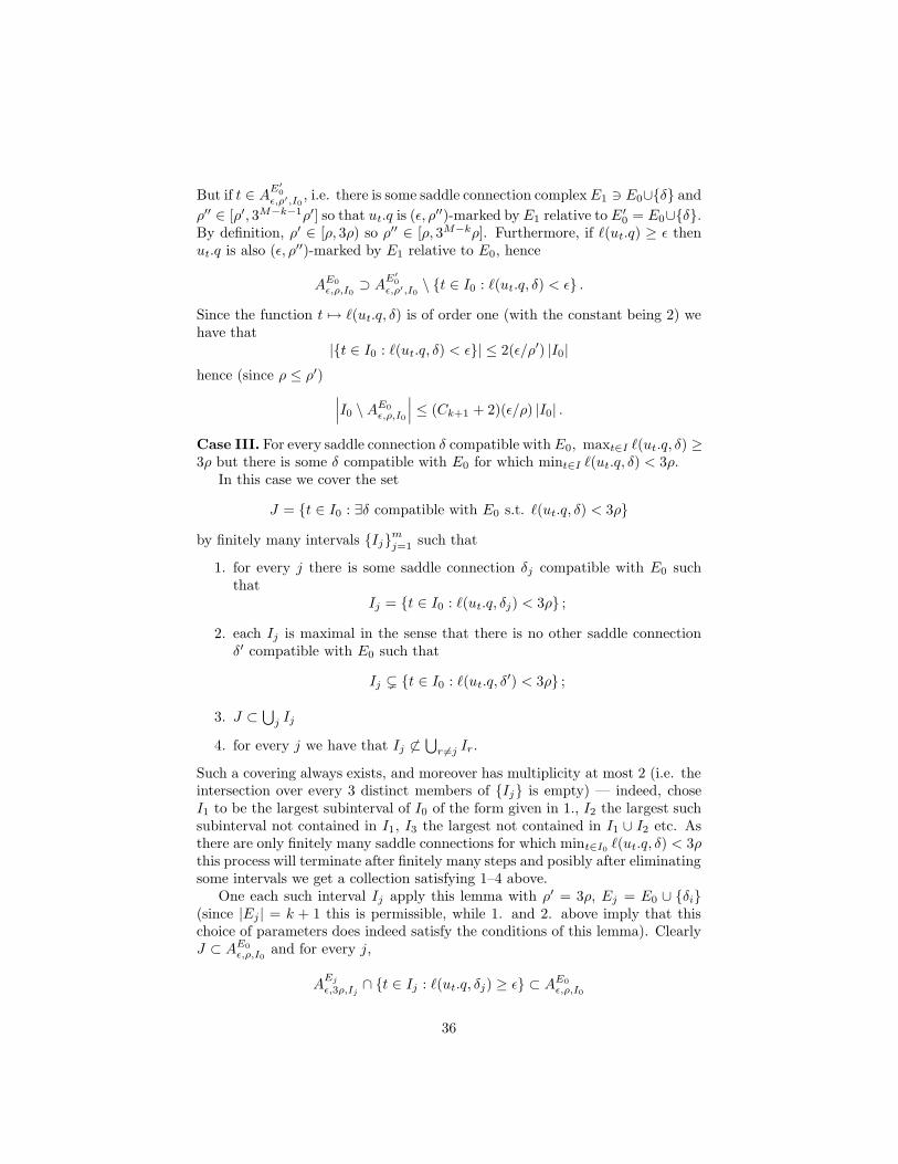
Case III. For every saddle connection δ compatible with E0, maxt∈I `(ut.q, δ) ≥3ρ but there is some δ compatible with E0 for which mint∈I `(ut.q, δ) < 3ρ.

In this case we cover the set

J = t ∈ I0 : ∃δ compatible with E0 s.t. `(ut.q, δ) < 3ρ

by finitely many intervals Ijmj=1 such that

1. for every j there is some saddle connection δj compatible with E0 suchthat

Ij = t ∈ I0 : `(ut.q, δj) < 3ρ ;

2. each Ij is maximal in the sense that there is no other saddle connectionδ′ compatible with E0 such that

Ij ( t ∈ I0 : `(ut.q, δ′) < 3ρ ;

3. J ⊂ ⋃j Ij

4. for every j we have that Ij 6⊂ ⋃r 6=j Ir.

Such a covering always exists, and moreover has multiplicity at most 2 (i.e. theintersection over every 3 distinct members of Ij is empty) — indeed, choseI1 to be the largest subinterval of I0 of the form given in 1., I2 the largest suchsubinterval not contained in I1, I3 the largest not contained in I1 ∪ I2 etc. Asthere are only finitely many saddle connections for which mint∈I0 `(ut.q, δ) < 3ρthis process will terminate after finitely many steps and posibly after eliminatingsome intervals we get a collection satisfying 1–4 above.

One each such interval Ij apply this lemma with ρ′ = 3ρ, Ej = E0 ∪ δi(since |Ej | = k + 1 this is permissible, while 1. and 2. above imply that thischoice of parameters does indeed satisfy the conditions of this lemma). ClearlyJ ⊂ AE0

ε,ρ,I0and for every j,

AEj

ε,3ρ,Ij∩ t ∈ Ij : `(ut.q, δj) ≥ ε ⊂ AE0

ε,ρ,I0

36

hence∣∣∣I0 \AE0

ε,ρ,I0

∣∣∣ ≤∑

j

∣∣∣Ij \AEj

ε,3ρ,Ij

∣∣∣ +∑

j

|t ∈ Ij : `(ut.q, δj) ≥ ε|

≤∑

j

(2 + Ck+1)(ε/3ρ) |Ij | ≤ (2 + Ck+1)(ε/ρ) |I0| .

This completes the inductive proof.

Lemma A.11. Suppose that t0 ∈ [0, T ] is εi, ρi-marked for loops by Ei fori = 1, 2, with ρ2 < ε1 < ρ1 < ρ0. Then S(E2) ⊆ S(E1). If S(E2) = S(E1) thenS(E1) contains no essential loops.

Proof. By definition of ε1, ρ1-marked for loops, E1 and ut.q satisfy the conditionsof Lemma A.6 with θ = 3ρ1. Therefore any saddle connection δ intersecting∂S(e1) satisfies `(ut.q, δ) ≥ `(ut.q, E1) > ρ1: so it cannot be in E2. Similarly,since by definition of ε1, ρ1-marked, any δ with `(ut.q, δ) ≤ `(ut.q, E1) has tointersect some saddle connection of E1. We conclude that every δ ∈ E2 is inS(E1) and therefore S(E2) ⊂ S(E1).

Assume that S(E1) contains an essential saddle connection loop. Since(for appropriate choice of ρ0) Proposition A.5 implies that S(E1) ( S, byLemma A.7 we have that ∂S(E1) contains an essential saddle connection loop,say E′

1.Since E1 gives an ε1, ρ1-marking for loops, one of the saddle connections in

E′1, say δ′ has `(ut.q, δ

′) > ε1. Since ε1 > ρ2 this saddle connection δ′ ∈ ∂S(E1)is not in E2 and it follows that S(E2) ( S(E1).

Proof of Theorem A.4. Suppose that q ∈ Q1M, T > 0 and ε < ρ < ρ0 satisfy(A.2), with ρ0 as in Proposition A.5. By appropriate choice of constant in (A.3),this equation can be made to be clearly true for ε ≥ 3−M(M+1)ρ, so we may aswell assume that ε < 3−M(M+1)ρ.

Let η = (ε/ρ)1/M+1, M being as before the maximal cardinality of a saddleconnection complex on S.

For every k = 0, . . . ,M let ρ(k) = 3−Mηkρ and ε(k) = ηk+1ρ. We apply

Proposition A.9 for each pair ε(k), ρ(k) and deduce that there is a set Alooptotal ⊂

[0, T ] with∣∣∣[0, T ] \Aloop

total

∣∣∣ < C ′ηT so that for every t ∈ Alooptotal, there is a ε(k), ρ

′(k)-

marking of ut.q by a saddle connection complex E(k)t , with ρ(k) ≤ ρ′(k) ≤ 3Mρ(k).

Note that for any k ≥ 1, we have 3Mρ(k) < εk−1.By Lemma A.11 and Proposition A.5,

S ⊃ S(E(0)t ) ⊃ S(E

(1)t ) ⊃ · · · ⊃ S(E

(M)t ).

Since there can be at most M compatible saddle connections on S at leastone of these inclusions must actually be equality, and hence (again invoking

37

Lemma A.11) for some k0, S(E(k0)t ) does not contain any essential saddle

connection loops.Suppose now that E is an essential saddle connection loop with `(ut.q, E) <

ε. Lemma A.6 implies that for any δ ∈ E intersecting S(E(k0)t ) `(ut, δ) ≥ ρ(k0);

the maximallity of S(E(k0)t ) implies a similar inequality if δ is compatible with

E(k0)t ), and so the only possibility is E ⊂ S(E

(k0)t ). But this is a contradiction

because S(E(k)) contains no essential saddle connection loops.

It follows that for every t ∈ Alooptotal there is no no essential saddle connection

loop E with `(ut.q, E) < ε.

38

References

[BM] R. Bowen and B. Marcus. Unique ergodicity for horocycle foliations.Israel J. Math. 26(1977), 43–67.

[Ca] K. Calta. Veech surfaces and complete periodicity in genus 2. J.Amer.Math. Soc. 17(2004), 871–908.

[Dani] S. G. Dani. Invariant measure of horospherical flows and noncompacthomogeneous spaces. Invent. math. 47(1978), 101–138.

[FLP] A. Fathi, F. Laudenbach, and V. Poenaru. Travaux de Thurston sur lessurfaces. Asterisque, volume 66–67, 1979.

[For] G. Forni. Deviation of ergodic averages for area-preserving flows onsurfaces of higher genus. Ann. of Math. (2) 155(2002), 1–103.

[Gd] F. Gardiner. Teichmuller Theory and Quadratic Differentials. WileyInterscience, 1987.

[GM] F. Gardiner and H. Masur. Extremal length geometry of Teichmullerspace. Complex Variables Theory Appl. 16(1991), 209–237.

[Ha] U. Hamenstadt. Bernoulli measures for the Teichmuller flow. preprint(50 pages).

[HP] J. L. Harer and R. C. Penner. Combinatorics of Train Tracks, volume125 of Annals of Math. Studies. Princeton University Press, 1992.

[HM] J. Hubbard and H. Masur. Quadratic differentials and foliations. ActaMath. 142(1979), 221–274.

[KMS] S. Kerckhoff, H. Masur, and J. Smillie. Ergodicity of billiard flows andquadratic differentials. Ann. of Math. 124(1986), 293–311.

[KM] D. Y. Kleinbock and G. A. Margulis. Flows on homogeneous spaces andDiophantine approximation on manifolds. Ann. of Math. (2) 148(1998),339–360.

[LS] F. Ledrappier and O. Sarig. Invariant measures for the horocycle flowon periodic hyperbolic surfaces. To appear in Israel J. Math (25 pages).

[Le] G. Levitt. Foliations and Laminations on Hyperbolic Surfaces. Topology22(1983), 119–135.

[Mar] G. A. Margulis. On some aspects of the theory of Anosov systems.Springer Monographs in Mathematics. Springer-Verlag, Berlin, 2004.With a survey by Richard Sharp: Periodic orbits of hyperbolic flows,Translated from the Russian by Valentina Vladimirovna Szulikowska.

[Mas1] H. Masur. Interval exchange transformations and measured foliations.Ann. of Math. 115(1982), 169–200.

39

[Mas2] H. Masur. The Teichmuller flow is Hamiltonian. Proc. Amer. Math.Soc. 123(1995), 3739–3747.

[MS] H. Masur and J. Smillie. Hausdorff dimension of the set of nonergodicfoliations. Annals of Math. 134(1991), 455–543.

[Mc] C. McMullen. Dynamics of SL2(R) over moduli space in genus 2. Toappear in Annals of Math.

[MW] Y. Minsky and B. Weiss. Nondivergence of horocycle flows on modulispaces. J. reine angew. Math. 552(2002), 131–177.

[Pap] A. Papadopoulos. Geometric intersection functions and Hamiltonianflows on the space of measured foliations of a surface. Pacific J. Math.124(1986), 375–402.

[Ra1] M. Ratner. On Raghunathan’s measure conjecture. Annals of Math.134(1991), 545–607.

[Ra2] M. Ratner. Raghunathan’s conjectures for SL(2,R). Israel J. Math80(1992), 1–31.

[Ro] T. Roblin. Ergodicity and uniform distributions in negative curvature.Mem. Soc. Math. Fr., No. 95, 2003.

[Str] K. Strebel. Quadratic Differentials. Springer-Verlag, 1984.

[Th] W. P. Thurston. Geometry and Topology of Three-Manifolds. LectureNotes, Princeton University, 1979.

[V1] W. Veech. The Teichmuller geodesic flow. Ann. of Math. 124(1986),441–530.

[V2] W. Veech. Measures supported on the set of uniquely ergodic directionsof an arbitrary holomorphic 1-form. Ergodic Theory Dynam. Systems19(1999), 1093–1109.

40