1

Ergodic Exploration of Distributed InformationLauren M. Miller,∗1 Yonatan Silverman,1 Malcolm A. MacIver,1,2 and Todd D. Murphey1

Abstract—This paper presents an active search trajectorysynthesis technique for autonomous mobile robots with nonlinearmeasurements and dynamics. The presented approach uses theergodicity of a planned trajectory with respect to an expectedinformation density map to close the loop during search. Theergodic control algorithm does not rely on discretization ofthe search or action spaces, and is well posed for coveragewith respect to the expected information density whether theinformation is diffuse or localized, thus trading off betweenexploration and exploitation in a single objective function. Asa demonstration, we use a robotic electrolocation platform toestimate location and size parameters describing static targets inan underwater environment. Our results demonstrate that theergodic exploration of distributed information (EEDI) algorithmoutperforms commonly used information-oriented controllers,particularly when distractions are present.

Index Terms—Information-Driven Sensor Planning, SearchProblems, Biologically-Inspired Robots, Motion Control

I. INTRODUCTION

IN the context of exploration, ergodic trajectory optimiza-tion computes control laws that drive a dynamic system

along trajectories such that the amount of time spent inregions of the state space is proportional to the expectedinformation gain in those regions. Using ergodicity as a metricencodes both exploration and exploitation—both the need fornonmyopic search when variance is high and convexity islost, as well as myopic search when variance is low and theproblem is convex. By encoding these needs into a metric [1],generalization to nonlinear dynamics is possible using toolsfrom optimal control. We show here that different dynamicalsystems can achieve nearly identical estimation performanceusing EEDI.

The SensorPod robot (Fig. 1a), which we use as a motivatingexample and an experimental platform in Section V, measuresdisturbances in a self-generated, weak electric field. Thissensing modality, referred to as electrolocation, is inspired bya type of freshwater tropical fish (Fig. 1b, [2], [3], [4]), andrelies on the coupled emission and detection of a weak electricfield. Electrolocation is ideally suited for low velocity, mobilevehicles operating in dark or cluttered environments [5], [6],[4]. The sensing range for electrolocation is small, however,so the fish or robot must be relatively close to an object tolocalize it. Also, as the sensors are rigid with respect to thebody, the movement of those sensors involves the dynamics of

1Department of Mechanical Engineering, 2Department of BiomedicalEngineering, Northwestern University, Evanston, Illinois, USA (∗e-mail:LMiller@u.northwestern.edu)

This work was supported by Army Research Office grant W911NF-14-1-0461, NSF grants IOB-0846032, CMMI-0941674, CMMI-1334609 and Officeof Naval Research Small Business Technology Transfer grants N00014-09-M-0306 and N00014-10-C0420 to M.A.M.

the entire robot. As we will see in Section IV, the measurementmodel for electrolocation is also highly nonlinear and thedynamics of both biological fish and underwater robots aregenerally nonlinear. Consideration of sensor physics and robotdynamics when planning exploration strategies is thereforeparticularly important. The same applies to many near-fieldsensors such as tactile sensors, ultra-shortwave sonar, andmost underwater image sensors (e.g. [7]). Experiments carriedout using the SensorPod robot demonstrate that the ergodicexploration of distributed information (EEDI) algorithm issuccessful in several challenging search scenarios where otheralgorithms fail.

The contributions of this paper can be summarized as follows:

1) application of ergodic exploration for general, nonlin-ear, deterministic control systems to provide closed-loop coverage with respect to the evolving expected

(a) The SensorPod robot (white cylinder at end of vertical Z stage) is used todemonstrate EEDI for active search.

(b) Apteronotus albifrons (photograph courtesy of Per Erik Sviland.)

Fig. 1. The SensorPod (a) uses a sensing modality inspired by weakly electricfish such as the black ghost knifefish (b). The SensorPod is mounted on a4DOF gantry and submerged within a 1.8 m x 2.4 m x 0.9 m (l,w,h) tank(see multimedia attachment).

arX

iv:1

708.

0935

2v1

[cs

.RO

] 3

0 A

ug 2

017

2

information density, and2) validation of ergodic search in an experimental and

simulated underwater sensing setting. We demonstrateboth that ergodic search performs as well as alternativealgorithms in nominal scenarios, and that ergodic searchoutperforms alternatives when distractors are present.

Section II begins with a discussion of related work. Ergodic-ity as an objective for active sensing is presented in Section III,including the benefits and distinguishing features of ergodictrajectory optimization. Section III-B includes an overview ofergodic trajectory optimization. In Section IV, we describe theSensorPod experimental platform and nonlinear measurementmodel, and introduce the stationary target localization taskused to demonstrate EEDI. We also discuss the components ofclosed-loop EEDI for target localization using the SensorPodin Section IV. In Section V, we present data from multipleestimation scenarios, including comparison to several alterna-tive algorithms, and closed-loop EEDI implementation usingdifferent dynamic models for the SensorPod. We also includea multimedia video attachment with an extended descriptionof the SensorPod platform and measurement model used inSections IV and V, and an animated overview of the steps ofthe EEDI algorithm for this system.

II. MOTIVATION & RELATED WORK

The ability to actively explore and respond to uncertain sce-narios is critical in enabling robots to function autonomously.In this paper, we examine the problem of control designfor mobile sensors carrying out active sensing tasks. Ac-tive sensing [8], [9] or sensor path planning [10], refersto control of sensor parameters, such as position, to ac-quire information or reduce uncertainty. Applications includeprioritized decision making during search and rescue [11],[12], inspection for flaws [13], mine detection [10], objectrecognition/classification [14], [15], [16], next-best-view prob-lems for vision systems [17], [18], [19], and environmen-tal modeling/field estimation [20], [21], [22]. Planning forsearch/exploration is challenging as the planning step neces-sarily depends not only on the sensor being used but on thequantity being estimated, such as target location versus targetsize. Methods for representing and updating the estimate andassociated uncertainty—the belief state—and a way of usingthe belief state to determine expected information are thereforerequired.

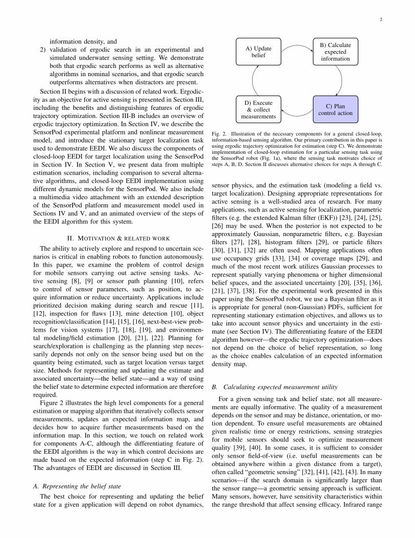
Figure 2 illustrates the high level components for a generalestimation or mapping algorithm that iteratively collects sensormeasurements, updates an expected information map, anddecides how to acquire further measurements based on theinformation map. In this section, we touch on related workfor components A-C, although the differentiating feature ofthe EEDI algorithm is the way in which control decisions aremade based on the expected information (step C in Fig. 2).The advantages of EEDI are discussed in Section III.

A. Representing the belief state

The best choice for representing and updating the beliefstate for a given application will depend on robot dynamics,

A) Updatebelief

B) Calculateexpected

information

C) Plancontrol action

D) Execute& collect

measurements

Fig. 2. Illustration of the necessary components for a general closed-loop,information-based sensing algorithm. Our primary contribution in this paper isusing ergodic trajectory optimization for estimation (step C). We demonstrateimplementation of closed-loop estimation for a particular sensing task usingthe SensorPod robot (Fig. 1a), where the sensing task motivates choice ofsteps A, B, D. Section II discusses alternative choices for steps A through C.

sensor physics, and the estimation task (modeling a field vs.target localization). Designing appropriate representations foractive sensing is a well-studied area of research. For manyapplications, such as active sensing for localization, parametricfilters (e.g. the extended Kalman filter (EKF)) [23], [24], [25],[26] may be used. When the posterior is not expected to beapproximately Gaussian, nonparametric filters, e.g. Bayesianfilters [27], [28], histogram filters [29], or particle filters[30], [31], [32] are often used. Mapping applications oftenuse occupancy grids [33], [34] or coverage maps [29], andmuch of the most recent work utilizes Gaussian processes torepresent spatially varying phenomena or higher dimensionalbelief spaces, and the associated uncertainty [20], [35], [36],[21], [37], [38]. For the experimental work presented in thispaper using the SensorPod robot, we use a Bayesian filter as itis appropriate for general (non-Gaussian) PDFs, sufficient forrepresenting stationary estimation objectives, and allows us totake into account sensor physics and uncertainty in the esti-mate (see Section IV). The differentiating feature of the EEDIalgorithm however—the ergodic trajectory optimization—doesnot depend on the choice of belief representation, so longas the choice enables calculation of an expected informationdensity map.

B. Calculating expected measurement utility

For a given sensing task and belief state, not all measure-ments are equally informative. The quality of a measurementdepends on the sensor and may be distance, orientation, or mo-tion dependent. To ensure useful measurements are obtainedgiven realistic time or energy restrictions, sensing strategiesfor mobile sensors should seek to optimize measurementquality [39], [40]. In some cases, it is sufficient to consideronly sensor field-of-view (i.e. useful measurements can beobtained anywhere within a given distance from a target),often called “geometric sensing” [32], [41], [42], [43]. In manyscenarios—if the search domain is significantly larger thanthe sensor range—a geometric sensing approach is sufficient.Many sensors, however, have sensitivity characteristics withinthe range threshold that affect sensing efficacy. Infrared range

3

sensors, for example, have a maximum sensitivity region [44],and cameras have an optimal orientation and focal length [45].

There are several different entropy-based measures frominformation theory and optimal experiment design that can beused to predict expected information gain prior to collectingmeasurements. Shannon entropy has been used to measureuncertainty in estimation problems [9], [15], [17], [19], as wellas entropy-related metrics including Renyi Divergence[24],[8], mutual information, [11], [14], [42], [46], [47], [35], [31],[48], entropy reduction or information gain maximization [49],[13]. In our problem formulation we use Fisher information[50], [51], [52], [53] to predict measurement utility. Oftenused in maximum likelihood estimation, Fisher informationquantifies the ability of a random variable, in our case ameasurement, to estimate an unknown parameter [54], [51],[50]. Fisher information predicts that the locations where theratio of the derivative of the expected signal to the variance ofthe noise is high will give more salient data (see Appendix Band the multimedia attachment), and thus will be more usefulfor estimation.

In this paper, the Bayesian update mentioned in Section II-Aand the use of Fisher information to formulate an informationmap are tools that allow us to close the loop on ergodic control(update the map, step A in Fig. 2), in a way that is appropriatefor the experimental platform and search objective (see Ap-pendix A). The Bayesian update and the Fisher informationmatter only in that they allow us to create a map of expectedinformation for the type of parameter estimation problemspresented in the examples in Section V. Ergodic explorationcould, however, be performed over the expected informationcalculated using different methods of representing the beliefand expected information, and for different applications suchas those mentioned in II-A.

C. Control for information acquisition

In general, the problem of exhaustively searching for anoptimally informative solution over sensor state space andbelief state is a computationally intensive process, as it isnecessary to calculate an expectation over both the belief andthe set of candidate control actions [24], [46], [35], [55].Many algorithms therefore rely on decomposing/discretizingthe search space, the action space, or both, and locallyselecting the optimal sensing action myopically (selectingonly the optimal next configuration or control input) [8],[25]. The expected information gain can, for example, belocally optimized by selecting a control action based on thegradient of the expected information [47], [30], [32], [33].As opposed to local information maximization, a sensor canbe controlled to move to that state which maximizes theexpected information globally over a bounded workspace [17],[56], [50], [28], [26]. Such global information maximizingstrategies are generally less sensitive to local minima thanlocal or gradient based strategies, but can result in longer,less efficient trajectories when performed sequentially [31],[29]. While myopic information maximizing strategies havean advantage in terms of computational tractability, they aretypically applied to situations where the sensor dynamics

are not considered [17], [56], [50], [28], [26], and even theglobal strategies are likely to suffer when uncertainty is highand information diffuse (as argued in [57], [29], [37], whendiscussing re-planning periods), as we will see in Section V.

To avoid sensitivity of single-step optimization methods tolocal optima, methods of planning control actions over longertime horizons—nonmyopic approaches—are often used. Agreat deal of research in search strategies point out thatthe most general approach to solving for nonmyopic con-trol signals would involve solving a dynamic programmingproblem [35], [20], [37], which is generally computationallyintensive. Instead, various heuristics are used to approximatethe dynamic programming solution [20], [37], [36], [29].Variants of commonly used sampling-based motion plannersfor maximizing the expected information over a path for amobile sensor have also been applied to sensor path planningproblems [10], [49], [58], [23], [24], [59].

Search-based approaches are often not suitable for systemswith dynamic constraints; although they can be coupled withlow-level (e.g. feedback control) planners [60], [48], or dy-namics can be encoded into the cost of connecting nodes ina search graph (“steering” functions) [58], solutions are notguaranteed to be optimal even in a local sense—both in termsof the dynamics and the information—without introducingappropriate heuristics [20], [37], [36], [29]. As we will see inSection V-G, one of the advantages of EEDI is that it naturallyapplies to general, nonlinear systems. We take advantageof trajectory optimization techniques, locally solving for asolution to the dynamic programming problem—assuming thatthe current state of the system is approximately known.

Use of an ergodic metric for determining optimal controlstrategies was originally presented in [1] for a nonuniformcoverage problem. The strategy in [1] involves discretizingthe exploration time and solving for the optimal control inputat each time-step that maximizes the rate of decrease of theergodic metric. A similar method is employed in [61], using aMix Norm for coverage on Riemannian manifolds. While ourobjective function includes the same metric as [1], the optimalcontrol problem and applications are different, notably in thatwe compute the ergodic trajectory for the entire planningperiod T , and apply it to a changing belief state. Additionally,the feedback controllers derived in [1] are specific to linear,first- or second-order integrator systems, whereas our methodapplies to general, nonlinear dynamic systems.

III. ERGODIC OPTIMAL CONTROL

Ergodic theory relates the time-averaged behavior of asystem to the space of all possible states of the system, andis primarily used in the study of fluid mixing and commu-nication. We use ergodicity to compare the statistics of asearch trajectory to a map of expected information density(EID). The idea is that an efficient exploration strategy—thepath followed by a robot—should spend more time exploringregions of space with higher expected information, whereuseful measurements are most likely to be found. The robotshould not, however, only visit the highest information region(see Fig. 3b), but distribute the amount of time spent searching

4

(a) Ergodic trajectory

(b) Information maximizing trajectory

Fig. 3. Two candidate trajectories x(t) for exploring the EID (depicted aslevel sets) are plotted in (a) and (b), both from t = 0 to t = T . Ergodic controlprovides a way of designing trajectories that spend time in areas proportionalto how useful potential measurements are likely to be in those areas (a). This isin contrast to many alternative algorithms, which directly maximize integratedinformation gain over the trajectory based on the current best estimate, as in3b. As illustrated in 3a, A trajectory x(t) is ergodic with respect to the PDF(level sets) if the percentage of time spent in any subset N from t = 0 tot = T is equal to the measure of N ; this condition must hold for all possiblesubsets.

proportional to the overall EID (Fig. 3a). This is the keydistinction between using ergodicity as an objective and pre-vious work in active sensing (e.g. information maximization);the ergodic metric encodes the idea that, unless the expectedinformation density is a delta function, measurements shouldbe distributed among regions of high expected information.Information maximizing strategies (that are also nonmyopic)otherwise require heuristics in order to force subsequentmeasurements away from previously sampled regions so asnot to only sample the information maxima.

As mentioned in Section II, many commonly used algo-rithms for active sensing, e.g. [25], [33], [28], [62], involve aversion of the type of behavior illustrated in Fig. 3b, iterativelyupdating the EID and maximizing information gain basedon the current best estimate, whether or not that estimate iscorrect. While computationally efficient, globally informationmaximizing approaches are likely to fail if the current estimateof the EID is wrong. In Section V, for example, we show thateven when the information map is updated while calculatingthe information maximizing control, the estimate may gettrapped in a local maxima, e.g. when there is a distractorobject that is similar but not exactly the same as the targetobject.

Many sampling-based algorithms for information gatheringtherefore rely on heuristics related to assuming submodularitybetween measurements, e.g. assuming no additional informa-

tion will be obtained from a point once it has already beenobserved [35], [23], [58]. This assumption forces subsequentmeasurements away from previously sampled regions so asnot to only sample the information maxima. As anotherway to distribute measurements, many nonmyopic strategiesselect a set of waypoints based on the expected information,and drive the system through those waypoints using search-based algorithms [49], [42], [48], [41], [57], [38], [60]. Suchapproaches result in a predefined sequence that may or maynot be compatible with the system dynamics. If the ordering ofthe waypoints is not predefined, target-based search algorithmsmay require heuristics to avoid the combinatoric complexity ofa traveling salesman problem [63], [64]. In some cases, searchalgorithms are not well-posed unless both an initial and final(goal) position are specified [42], [20], which is not generallythe case when the objective is exploration.

Ergodic control enables how a robot searches a space to de-pend directly on the dynamics, and is well posed for arbitrarydynamical systems. In the case of nonlinear dynamics andnontrivial control synthesis, encoding the search ergodicallyallows control synthesis to be solved directly in terms of themetric, instead of in a hierarchy of problems (starting withtarget selection and separately solving for the control thatacquires those targets, for example [49], [42], [41], [57], [38],[60]). In ergodic trajectory optimization, the distribution ofsamples results from introducing heuristics into the trajectoryoptimization, but of encoding the statistics of the trajectory andthe information map directly in the objective. Using methodsfrom optimal control, we directly calculate trajectories thatare ergodic with respect to a given information density [65],[66]. It is noteworthy, however, that even if one wants to addwaypoints to a search objective, ergodic search is an effectivemeans to drive the system to each waypoint in a dynamicallyadmissible manner (by replacing each waypoint with a low-variance density function, thus avoiding the traveling salesmanproblem). Further, ergodic control can be thought of as a wayto generate a continuum of dynamically compatible waypoints;it is similar to [49], [42], [57], but allows the number ofwaypoints to go to ∞, making the control synthesis moretractable for a broad array of systems.

Many active sensing algorithms are formulated to eitherprioritize exploitation (choosing locations based on the currentbelief state) or exploration (choosing locations that reduceuncertainty in the belief state); they are best suited forgreedy, reactive sampling, requiring a prior estimate [23], orfor coverage [35], [67], [68]. Algorithms that balance bothexploration and exploitation typically involve encoding thetwo objectives separately and switching between them basedon some condition on the estimate, [69], [37], or defininga (potentially arbitrary) weighted cost function that balancesthe tradeoff between the two objectives [36], [60], [38], [22].Using ergodicity as an objective results in an algorithm thatis suitable for both exploration-prioritizing coverage samplingor exploitation-prioritizing “hotspot” sampling, without modi-fication (policy switching or user-defined weighted objectives[69], [37], [36], [60], [22]). Moreover, the ergodic metric canbe used in combination with other metrics, like a tracking costor a terminal cost, but does not require either to be well-posed.

5

A. Measuring Ergodicity

We use the distance from ergodicity between the time-averaged trajectory and the expected information densityas a metric to be minimized. We assume a bounded, n-dimensional workspace (the search domain) X ⊂ Rn definedas [0, L1] × [0, L2]... × [0, Ln]. We define x(t) as the sensortrajectory in workspace coordinates, and the density functionrepresenting the expected information density as EID(x).

The spatial statistics of a trajectory x(t) are quantified bythe percentage of time spent in each region of the workspace,

C(x) =1

T

∫ T

0

δ [x− x(t))] dt, (1)

where δ is the Dirac delta [1]. The goal is to drive the spatialstatistics of a trajectory x(t) to match those of the distributionEID(x); this requires choice of a norm on the differencebetween the distributions EID(x) and C(x). We quantifythe difference between the distributions, i.e. the distance fromergodicity, using the sum of the weighted squared distancebetween the Fourier coefficients φk of the EID, and thecoefficients ck of distribution representing the time-averagedtrajectory.1 The ergodic metric will be defined as E , as follows:

E(x(t)) =

K∈Zn∑k=0∈Zn

Λk [ck(x(t))− φk]2 (2)

where K is the number of coefficients calculated along eachof the n dimensions, and k is a multi-index (k1, k2, ..., kn).Following [1], Λk = 1

(1+||k||2)s is a weight where s = n+12 ,

which places larger weight on lower frequency information.Note that the notion of ergodicity used here does not strictly

require the use of Fourier coefficients in constructing anobjective function. The primary motivation in using the normon the Fourier coefficients to formulate the ergodic objective isthat it provides a metric that is differentiable with respect to thetrajectory x(t). This particular formulation is not essential—any differentiable method of comparing the statistics of adesired expected information density to the spatial distributiongenerated by a trajectory will suffice, however finding such amethod is nontrivial. The Kullback-Leibler (KL) divergence orJensen-Shannon (JS) divergence [21], for example, commonlyused metrics on the distance between two distributions, arenot differentiable with respect to the trajectory x(t).2 On theother hand, by first decomposing both distributions into theirFourier coefficients, the inner product between the transformand the expression for the time-averaged distribution results inan objective that is differentiable with respect to the trajectory.

1The Fourier coefficients φk of the distribution Φ(x) are computed usingan inner product, φk =

∫X φ(x)Fk(x)dx, and the Fourier coefficients of

the basis functions along a trajectory x(t), averaged over time, are calculatedas ck(x(t)) = 1

T

∫ T0 Fk(x(t))dt, where T is the final time and Fk is a

Fourier basis function.2Due to the Dirac delta in Eq. (1), the JS divergence ends up involving

evaluating the EID along the trajectory x(t). In general we do not expect tohave a closed form expression for the EID, so this metric is not differentiablein a way that permits trajectory optimization. Alternatively, replacing theDirac delta in Eq. (1) with a differentiable approximation (e.g. a Gaussian)would expand the range of metrics on ergodicity, but would introduceadditional computational expense of evaluating an N dimensional integralwhen calculating the metric and its derivative.

B. Trajectory Optimization

For a general, deterministic, dynamic model for a mobilesensor x(t) = f(x(t),u(t)), where x ∈ RN is the stateand u ∈ Rn the control, we can solve for a continuoustrajectory that minimizes an objective function based on boththe measure of the ergodicity of the trajectory with respect tothe EID and the control effort, defined as

J(x(t)) = γE [x(t)]︸ ︷︷ ︸ergodic cost

+

∫ T

0

1

2u(τ)TRu(τ)dτ︸ ︷︷ ︸control effort

. (3)

In this equation, γ ∈ R and R(τ) ∈ Rm×m are arbitrary designparameters that affect the relative importance of minimizingthe distance from ergodicity and the integrated control effort.The choice of ratio of γ to R plays the exact same role inergodic control as it does in linear quadratic control and othermethods of optimal control; the ratio determines the balancebetween the objective—in this case ergodicity—and the con-trol cost of that objective. Just as in these other methods,changing the ratio will lead to trajectories that perform betteror worse with either more or less control cost.

In [65] we show that minimization of Eq. (3) can beaccomplished using an extension of trajectory optimization[70], and derive the necessary conditions for optimality.The extension of the projection-based trajectory optimizationmethod from [70] is not trivial as the ergodic metric is nota Bolza problem; however, [65] proves that the first-orderapproximation of minimizing Eq. (3) subject to the dynamicsx(t) = f(x(t),u(t)) is a Bolza problem and that trajectoryoptimization can be applied to the ergodic objective. Theoptimization does not require discretization of search space orcontrol actions in space or time. While the long time horizonoptimization we use is more computationally expensive thanthe myopic, gradient-based approach in [1], each iteration ofthe optimization involves a calculation with known complexity.The EID map and ergodic objective function could, however,also be utilized within an alternative trajectory optimizationframework (e.g. using sequential quadratic programming).Additionally, for the special case of x = u, sample-basedalgorithms [58] may be able to produce locally optimal ergodictrajectories that are equivalent (in ergodicity) to the solutionobtained using trajectory optimization methods; this wouldnot however, be the case for general, nonlinear dynamicsx(t) = f(x(t),u(t)).

Ergodic optimal control allows for the time of exploration tobe considered as an explicit design variable. It can, of course,be of short duration or long duration, but our motivation islargely long duration. The idea is that one may want to executea long exploration trajectory prior to re-planning. The moststraightforward motivation is that integrating measurementsand updating the belief may be the more computationallyexpensive part of the search algorithm [31], [29], [23], [37].Overly reactive/adaptive strategies—strategies that incorporatemeasurements as they are received—are also likely to performpoorly when the estimate uncertainty is high [57], [29], [37] orin the presence of (inevitable) modeling error. If, for example,the measurement uncertainty is not perfectly captured by the

6

measurement model, the idealized Bayesian update can leadto overly reactive control responses. Instead, one may wish totake enough data such that the central limit theorem can beapplied to the measurement model, so that the measurementmodel is only anticipated to be applicable on average over thelength of the exploratory motion [71]. Future work will involveexploring the effects of reducing the re-planning horizon onthe success of the estimation algorithm.

C. Assumptions: Ergodic Trajectory Optimization

Ergodic trajectory optimization requires a controllable mo-tion model for the robot, and an expected information densityfunction defined over the sensor state space. The motionmodel can be nonlinear and/or dynamic, one of the primarybenefits of a trajectory optimization approach. For this paperwe consider calculating search trajectories in one and twodimensions (although the sensor dynamics can be higherdimensional). The trajectory optimization method can be ex-tended to search in higher dimensional search spaces such asR3 and SE(2), so long as a Fourier transform [72] existsfor the manifold [66]. We consider only uncertainty of staticenvironmental parameters (e.g. fixed location and radius ofan external target) assuming noisy measurements. We assumedeterministic dynamics.

IV. EXPERIMENTAL METHODS: SEARCH FOR STATIONARYTARGETS USING THE SENSORPOD ROBOT

Although ergodic trajectory optimization is general tosensing objectives with spatially distributed information, wedescribe an application where the belief representation andexpected information density (EID) calculation (steps A, B,and D in Fig. 2) are chosen for active localization of stationarytargets using the SensorPod robot. This allows us to experi-mentally test and validate a closed-loop version of the ergodicoptimal control algorithm, described in Section III, againstseveral established alternatives for planning control algorithmsbased on an information map.

Inspired by the electric fish, the SensorPod (Fig. 1a) has twoexcitation electrodes that create an oscillating electric field. Weuse a single pair of voltage sensors—hence, a one-dimensionalsignal —on the body of the SensorPod to detect perturbationsin the field due to the presence of underwater, stationary,nonconducting spherical targets. The expected measurementdepends on the location, size, shape, and conductivity of anobject as well as the strength of the electric field generatedby the robot; for details, see [73]. The perturbed electricfields and resulting differential measurements for targets intwo locations relative to the SensorPod are shown in Fig. 4,and the differential voltage measurement is plotted in Fig. 5a.Figure 5b shows the expected differential measurement fortwo candidate sensor trajectories. The multimedia attachmentprovides additional intuition regarding the SensorPod andand the observation model. The solid line trajectory is moreinformative, as measured using Fisher Information, than thedashed line; our goal is to automatically synthesize trajectoriesthat are similarly more informative.

(a) +0.2 mV expected voltage difference between the sensors on the SensorPodfor a target located as shown.

(b) -0.2 mV expected voltage difference between the sensors (A-B) on theSensorPod for a target located as shown.

Fig. 4. The SensorPod (grey) measures the difference between the fieldvoltage at the two sensors (A-B). The field is generated by two excitationelectrodes on the SensorPod body. The field (simulated isopotential linesplotted in black) changes in the presence of a target with different conductivitythan the surrounding water. The 0V line is bolded. The perturbation cause bythe same object results in a different differential measurement between sensorsA and B based on the position of the object relative to the SensorPod. Formore information and an animation of this plot, please see the multimediavideo attachment. Note that the SensorPod is not measuring the field itself(which is emitted by, and moves with, the robot), but the voltage differentialbetween two sensors induced by disturbances in the field.

(a) The expected differential voltage measurement (A-B from Fig. 4) is plottedas a function of robot centroid for a target (pink) located at X,Y=(0,0). Twopossible SensorPod trajectories are plotted in black (solid and dashed). Thetarget is placed below the robot’s plane of motion to prevent collisions.

(b) Simulated differential voltage measurements for the trajectories in (a) areplotted as a function of time.

Fig. 5. Measurements collected by the SensorPod have a nonlinear and non-unique mapping to target location. The dashed trajectory in Fig. 5a yieldsuninformative measurements (possible to observe for many potential targetlocations); the solid trajectory in Fig. 5a, produces a series of measurementsthat are unique for that target position, and therefore useful for estimation.

The objective in the experimental results presented in Sec-tion V is to estimate a set of unknown, static, parametersdescribing individual spherical underwater targets. Details and

7

assumptions for implementation of both the Bayesian filterand the calculation of the expected information density forthe SensorPod robot, including for the multiple target case,can be found in Appendix A; an overview of the algorithm isprovided here, corresponding to the diagram in Fig. 2). For agraphical, animated overview of the algorithm, please also seethe attached multimedia video.

The algorithm is initialized with the sensor state at the initialtime x(0) and an initial probability distribution p(θ) for theparameters θ. We represent and update the parameter estimateusing a Bayesian filter, which updates the estimated beliefbased on collected measurements (Fig. 2, step A). The initialdistribution can be chosen based on prior information or, inthe case of no prior knowledge, assumed to be uniform onbounded domains. At every iteration of the EEDI algorithm,the EID is calculated by taking the expected value of the Fisherinformation with respect to the belief p(θ) (Fig. 2, step B).For estimation of multiple parameters, we use the D-optimalitymetric on the expected Fisher information matrix, equivalentto maximizing the determinant of the expected information[51].3 In Fig. 6, the corresponding EIDs for two differentbelief maps for 2D target location (Figs. 6b and 6e), as wellas the EID for estimating both 2D target location and targetradius (6c), are shown. The EID is always defined over thesensor configuration space (2D), although the belief map maybe in a different or higher dimensional space (e.g. over the2D workspace and the space of potential target radii). Thenormalized EID is used to calculate an optimally ergodicsearch trajectory for a finite time horizon (Fig. 2, step C). Thetrajectory is then executed, collecting a series of measurements(Fig. 2, step D, for time T ). Measurements collected in stepD are then used to update the belief p(θ), which is then usedto calculate the EID in the next EEDI iteration. The algorithmterminates when the norm on the of the estimate falls belowa specified value.

For localizing and estimating parameters for multiple tar-gets, we initialize the estimation algorithm by assuming thatthere is a single target present, and only when the norm on thevariance of the parameters describing that target fall below thetolerance ε do we introduce a second target into the estimation.The algorithm stops searching for new targets when one of twothings happen: 1) parameters for the last target added convergeto values that match those describing a target previouslyestimated (this would only happen if all targets have beenfound, as the EID takes into account expected measurementsfrom previous targets), or 2) parameters converge to an invalidvalue (e.g. a location outside of the search domain), indicatingfailure. The algorithm terminates when the entropy of thebelief map for all targets falls below a chosen value; for the0 target case, this means that the SensorPod has determinedthat there are no objects within the search space. Note that theEID for new targets takes into account the previously locatedtargets

3Note that alternative choices of optimality criteria may result in differentperformance for different problems based on, for example, the conditioningof the information matrix. D-optimality is commonly used for similar appli-cations and we found it to work well experimentally; however the rest of theEEDI algorithm is not dependent on this choice of optimality criterion.

(a) A low-variance PDFof 2D target location

(b) EID for target loca-tion for the PDF in (a)

(c) EID for target loca-tion and radius.

(d) A higher-variancePDF of 2D target location.

(e) EID map for the PDFin (c)

Fig. 6. The EID is dependent on the measurement model and the currentprobabilistic estimate. Figures 6b, 6c, 6e show examples of the EID fordifferent PDFs and estimation tasks for the SensorPod measurement model.For 6c, the projection of the corresponding PDF (defined in three-dimensions)onto the 2D location space would be similar to (a). The EID is calculatedaccording to Eq. (12). In all cases, calculation of the EID produces a mapover the search domain, regardless of the estimation task.

A. Assumptions: stationary target localization using the Sen-sorPod (EEDI example)

We make a number of assumptions in choosing steps A,B, and D in Fig. 2, detailed in Appendix A. We assume ameasurement is made according to a known, differentiablemeasurement model (a function of sensor location and pa-rameters), and assume the measurements have zero-mean,Gaussian, additive noise.4 We assume independence betweenindividual measurements, given that the SensorPod state isknown and the measurement model is not time-varying. Mea-surement independence is commonly assumed, for examplein occupancy grid problems [29], however more sophisticatedlikelihood functions that do not rely on this assumption of in-dependence [74] could be used without significantly changingthe structure of the algorithm.

For the single target case, we maintain a joint probabilitydistribution for parameters describing the same target as theyare likely to be highly correlated. In order to make the problemof finding an arbitrary number of objects tractable, we assumethat the parameters describing different targets are independentand that a general additive measurement model may be used,similar to [24], [75], [28]. Although the voltage perturbationsfrom multiple objects in an electric field do not generally addlinearly, we make the assumption that the expected measure-ment for multiple objects can be approximated by summing theexpected measurement for individual objects, which simplifiescalculations in Appendix A.5 While the computation of FisherInformation and the likelihood function used for the Bayesian

4Related work in active electrosense has shown that zero mean Gaussianis a reasonable assumption for sensor noise [5].

5Additional experimental work (not shown), demonstrated that at a min-imum of 6 cm separation between objects, there is no measurable errorusing this approximation; in the experimental and simulated trials, we usea minimum separation of 12 cm.

8

Top View of Tank

Meters

Meters

Sensor Pod

θd

yd

θ

y

x

−0.3 −0.2 −0.1 0 0.1 0.2 0.3−0.3

−0.2

−0.1

0

0.1

0.2

0.3

(a) For estimation of target location in 1D (Sec-tions V-A and V-E), the target object (green) wasplaced at a fixed distance of y = 0.2 m fromthe SensorPod line of motion, and the distractor(pink) at yd = 0.25 m.

target meas.distractor meas.combined meas.

0.6 0.4 0.2 0.0 0.2 0.4 0.60.4

0.2

0.0

0.2

0.4

Sensor Position (m)

Diff

eren

tialM

easu

rem

ent(

mV)

(b) Expected voltage measurement over 1D sensor statefor the target (pink) and distractor (green) objects alone,and when both target and distractor are present (black).

Top View of Tank

Meters

Meters

Sensor Pod

θ2x

θ2y

θ1x

θ1y

yx

−0.3 −0.2 −0.1 0 0.1 0.2 0.3−0.3

−0.2

−0.1

0

0.1

0.2

0.3

(c) Example of tank configuration for 2D local-ization of two targets. For all trials, SensorPodand object locations are measured from thecenter of the tank.

Fig. 7. Targets were placed below the robot’s plane of motion to prevent collisions. The orientation of the robot is held constant. The voltage sensors sampleat 100 Hz, with an assumed standard deviation of 100 µV for the measurement noise, the experimentally observed noise level of the SensorPod sensors.

update depend on the assumptions mentioned above, theergodic optimal control calculations do not, and only dependon the existence of an EID map.

The SensorPod is attached to a 4-DOF gantry system, whichallows use of a kinematic model of the SensorPod in Eq.(3), i.e. the equations of motion for the experimental systemare x(t) = u(t), where x is the SensorPod position in1D (Sections V-A and V-E) or 2D (Sections V-B, V-C, andV-D). The kinematic model and 2D search space also enablecomparison with other search methods; however, it should benoted that EEDI is applicable to dynamic, nonlinear systemsas well, as will be demonstrated in simulation in Section V-G.

Ergodic trajectory optimization, presented in Section III,calculates a trajectory for a fixed-length time horizon T ,assuming that the belief, and therefore the EID map, remainsstationary over the course of that time horizon. In the followingexperiments, this means that each iteration of the closed loopalgorithm illustrated in Fig. 2 involves calculating a trajectoryfor a fixed time horizon, executing that trajectory in its entirety,and using the series of collected measurements to updatethe EID map before calculating the subsequent trajectory.The complete search trajectory, from initialization until ter-mination, is therefore comprised of a series of individualtrajectories of length T , where the belief and EID are updatedin between (this is also true for the alternative strategies usedfor comparison in Section V). The EID map could alternativelybe updated and the ergodic trajectory re-planned after eachmeasurement or subset of measurements, in a more traditionalreceding horizon fashion, or the time horizon (for planningand updating) could be optimized.

B. Performance assessment

In the experiments in Section V, we assess performanceusing time to completion and success rate. Time to completionrefers to the time elapsed before the termination criterionis reached, and a successful estimate obtained. We presentresults for time until completion as the slowdown factor.

The slowdown factor is a normalization based on minimumtime until completion for a particular set of experiments orsimulation. For a trial to be considered successful, the mean ofthe estimate must be within a specified range of the true targetlocation, and in Section V-C, the number of targets found mustbe correct. The tolerance used on the distance of the estimatedparameter mean to the true parameter values was 1 cm forthe 1D estimation experiments and 2 cm for 2D experiments.In both cases this distance was more than twice the standarddeviation used for our termination criterion.

A maximum run-time was enforced in all cases (100 sec-onds for 1D and 1000 seconds for 2D experiments). For simpleexperimental scenarios, e.g. estimation of the location of asingle target in 2D (Section V-B), these time limits werelonger than the time to completion all algorithms in simu-lation. Additional motivation for limiting the run time wereconstraints on the physical experiment, and the observationthat when algorithms failed they tended to fail in such away that the estimate variance never fell below a certainthreshold (excluding the random walk controller), and thesuccess criteria listed above could not be applied.

V. TRIAL SCENARIOS & RESULTS

Experiments were designed to determine whether the EEDIalgorithm performs at least as well as several alternativechoices of controllers in estimating of the location of station-ary target(s), and whether there were scenarios where EEDIoutperforms these alternative controllers, e.g. in the presenceof distractor objects or as the number of targets increases.Experiments in Sections V-A through V-D are performed usingthe kinematically controlled SensorPod robot and simulation,and these results are summarized in Section V-F. In SectionV-G, we transition to simulation-only trials to demonstrate suc-cessful closed-loop estimation of target location, but comparetrajectories and performance using three models of the robot;the kinematic model of the experimental system, a kinematicunicycle model, and a dynamic unicycle model.

9

In Sections V-A through V-D we compare the performanceof EEDI to the following three implementations of informationmaximizing controllers and a random walk controller: I.

1) Information Gradient Ascent Controller (IGA) TheIGA controller drives the robot in the direction of thegradient of the EID at a fixed velocity of 4 cm/s, inspiredby controllers used in [47], [30], [32], [33].

2) Information Maximization Controller (IM) The Sen-sorPod is controlled to the location of the EID maxi-mum, at a constant velocity for time T , similar to [56],[50], [28], [26].

3) Greedy Expected Entropy Reduction (gEER) At eachiteration, fifty locations are randomly selected, within afixed distance of the current position. The SensorPod iscontrolled to the location that maximizes the expectedchange in entropy, integrated over the time horizon T.6

This approach is similar to the method of choosingcontrol actions in [9], [8], [25], [38]

4) Random Walk (RW) The SensorPod executes a ran-domly chosen, constant velocity trajectory from thecurrent sensor position for time T , similar to [5].

The planning horizon T was the same for all controllers, sothat the same number of measurements is collected.

Alternative algorithms, for example a greedy gradient-basedcontroller (IGA) or a random walk (RW), produce control sig-nals with less computational overhead than the EEDI algorithmbecause the EEDI involves solving a continuous trajectoryoptimization problem and evaluating an additional measure onergodicity. In the next section we demonstrate several scenar-ios in which the tradeoff in computational cost is justified ifthe estimation is likely to fail or suffer significantly in termsof performance using less expensive control algorithms. Ad-ditionally, the alternative algorithms, while appropriate for thekinematically-controlled SensorPod robot, do not generalizein an obvious way to nonlinear dynamic models. This is oneof our reasons for desiring a measure of nonmyopic searchthat can be expressed as an objective function (i.e. ergodicity).Given an objective, optimal control is a convenient meansby which one makes dynamically dissimilar systems behavesimilarly to each other according to a metric of behavior. Inthe case of exploration, the measure is of coverage relative tothe EID—however it is constructed.

A. Performance comparison for 1D target estimation in thepresence of an unmodeled distractor

In this section, the robot motion is constrained to a singledimension, and the estimation objective is the 1D location θof a single, stationary target with known radius. A distractorobject is placed in the tank, as an unmodeled disturbance,in addition to the (modeled) target object. Both the targetand the distractor were identical non-conductive, 2.5 cmdiameter spheres, placed at different fixed distances fromthe SensorPod’s line of motion (see Fig. 7a). The voltage

6The expected entropy reduction isH(θ)−E[H(θ)|V +(t)] whereH(θ) =−

∫p(θ) log p(θ)dθ is the entropy of the unknown parameter θ [75], [46] and

V +(t) is the expected measurement, calculated for each candidate trajectoryx+(t), the current estimate p(θ), and the measurement model.

Tim

e (s

) Tim

e (s

)

0

01

2

3

4

5

6

7

8

8

16

0 0.5-0.5

0 0.5-0.5

1D Sensor Position (m)

SensorPod Path

1D Sensor Position (m)

EIDTarget Object

Distractor Object

(a) Simulation

Tim

e (s

) Tim

e (s

)

0

01

2

3

4

5

6

7

8

8

16

0 0.5-0.5

0 0.5-0.5

1D Sensor Position (m)

SensorPod Path

1D Sensor Position (m)

EIDTarget Object

Distractor Object

(b) Experiment

Fig. 8. Examples of closed-loop optimally ergodic search in simulation andexperiment. The EID is shown as a density plot in blue, and the searchtrajectory in red. The belief and trajectory are recalculated every second insimulation and every 8 seconds in experiment.

TABLE IPERFORMANCE MEASURES FOR ESTIMATION OF SINGLE TARGET

LOCATION IN 1D FOR 100 SIMULATED AND 10 EXPERIMENTAL TRIALS.RESULTS FOR TIME UNTIL COMPLETION (SLOWDOWN FACTOR) ARE ONLY

SHOWN FOR SUCCESSFUL TRIALS. SLOWDOWN FACTOR OF 1CORRESPONDS TO 15.2 S IN EXPERIMENT, 7.6 S IN SIMULATION.

Description EEDI gEER IM IGA RWExp. Success % 100 50 60 50 80Sim. Success % 100 60 71 66 99

Exp. Slowdown Factor 1 1.4 2.1 2.7 2.7Sim. Slowdown Factor 1 2.1 2.1 2.3 6.3

signal from the distractor object is similar but not identicalto that of the target (see Fig. 7b). Placing the distractor objectfurther from the SensorPod line of motion results in decreasedmagnitude and rate of change of the voltage trace. Introducingan unmodeled distractor even in a one-dimensional sensingtask was enough to illustrate differences in the performanceof the EEDI Algorithm and Algorithms I-IV.

We performed 100 trials in simulation and 10 in experiment,with the target position held constant and the distractor’sposition along the SensorPod’s line of motion randomized.7

The results for success rate and average slowdown factor(for successful trials), averaged over all trials in simulationand experiment, are summarized in Table I. The slowdownfactor is the average time until completion, normalized bythe minimum average time until completion in experiment orsimulation. Results presented in Table I demonstrate that theEEDI algorithm localizes the target successfully 100% of thetime, and does so more quickly than Algorithms I-IV.

Differences in time to completion between experimental andsimulated trials are due to experimental velocity constraints. Insimulation, the time horizon used for trajectory optimization,and therefore between PDF updates, was one T = 1 second. A

7 The only additional consideration in the experimental scenario was that thetank walls and the water surface have a non-negligible effect on measurements.We compensate for this by collecting measurements on a fine grid in an emptytank, and subtracting these measurements at each measurement point duringestimation.

10

Fig. 9. A progression of the estimate of the two-dimensional target location using the EEDI algorithm. As the algorithm progresses, collected measurementsevolve the estimate from a uniform distribution over the workspace (top-leftmost figure), to a concentrated distribution at the correct location. At each interval,the EID is calculated from the updated estimate, which is then used to calculate an ergodic search trajectory.

TABLE IIPERFORMANCE MEASURES FOR ESTIMATION OF SINGLE TARGET

LOCATION IN 2D FOR 10 SIMULATED AND 10 EXPERIMENTAL TRIALS.RESULTS FOR TIME UNTIL COMPLETION (SLOWDOWN FACTOR) ARE ONLY

SHOWN FOR SUCCESSFUL TRIALS. SLOWDOWN FACTOR OF 1CORRESPONDS TO 64 S IN EXPERIMENT, 65.2 S IN SIMULATION.

Description EEDI gEER RWExp. Success % 100 90 90Sim. Success % 100 100 100

Exp. Slowdown Factor 1 1.2 2.9Sim. Slowdown Factor 1 1.1 2.6

longer (T = 8 seconds) time horizon was used for experimen-tal trajectory optimization, avoiding the need to incorporatefluid dynamics in the measurement model; at higher velocitiesthe water surface is sufficiently disturbed to cause variationsin the volume of fluid the field is propagating through, causingunmodeled variability in sensor measurements.

Figure 8 shows experimental and simulated examples ofclosed-loop one-dimensional trajectories generated using theEEDI algorithm. Given no prior information (a uniform belief),the ergodic trajectory optimization initially produces uniform-sweep-like behavior. In the experimental trial shown in Fig.8b, the termination criteria on the variation of the PDFis reached in only two iterations of the EID algorithm, aresult of the longer time horizon and resulting higher densitymeasurements. The distributed sampling nature of the EEDIalgorithm can be better observed in the simulated exampleshown in Fig. 8a, where shorter time horizons and thereforemore sparse sampling over the initial sweep require moreiterations of shorter trajectories. As the EID evolves in Fig.8a, the shape of the sensor trajectory changes to reflect thedistribution of information. For example, the sensor visits thelocal information maximum resulting from voltage perturba-tions due to the target and the local information maximumdue to the distractor between 1 and 4 seconds. Experimentalresults for this trial were presented in [76].

B. Performance comparison for estimating the 2D location ofa single target

In this section, the robot is allowed to move through a 2Dworkspace and the objective was to compare the performance

of EEDI to gEER and RW for 2D, stationary target local-ization, i.e. θ = (θx, θy). No distractor object was present asthe difference in performance between algorithms was notableeven without introducing a distractor object. Fig. 7c shows anexample tank configuration for multiple target estimation in2D. We omit comparison to IGA and IM for 2D experiments;RW is the simplest controller to calculate and resulted in highsuccess percentage for 1D trials, and gEER, with performancesimilar to IGA and IM on average in 1D trials, is qualitativelysimilar to our approach and more commonly used.

Ten trials were run for each of the EEDI, gEER, and RWalgorithms, both in experiment and simulation, with the targetlocation randomly chosen. Figure 9 shows the convergence ofthe belief at 10 second intervals (T = 10), as well as thecorresponding EID and ergodic trajectory. The performancemeasures for experimental and simulated trials using theEEDI, gEER, and RW algorithms are shown in Table II. Insimulation, all three algorithms have 100% success rate, whilethe gEER and RW controllers have a 10% lower success ratein the experimental scenario. The gEER controller requiresroughly 10-20% more time to meet the estimation criteria,whereas the RW controller requires about 2-3 times more time.As mentioned in the previous section, although gEER performswell in this scenario, it did not perform as well with distractors.

C. Performance comparison for estimating the 2D location ofmultiple targets

Having demonstrated that the EEDI algorithm modestlyoutperforms gEER and drastically outperforms RW (in termsof time) for localizing a single, stationary target in 2D, wenext sought to compare EEDI performance localizing multipletargets (see Fig. 7c). We compare the EEDI algorithm tothe gEER and RW controllers, again leaving out IM andIGA because of their poor performance in Section V-A. Weperformed localization estimation for scenarios where therewere either 0, 1, 2, or 3 targets in the tank, all 2.5 cm diameter.We conducted 5 trials in simulation and experiment, for eachnumber of targets (with all locations selected randomly).Figure 10 shows the percentage of successful trials and averageslowdown factor as a function of the number of targets inthe tank. The slowdown factor is calculated by normalizing

11

(a) Experiment (b) Simulation

Fig. 10. Performance measures for estimation of multiple target locationsin 2D for five experimental and five simulated trials. Slowdown factor of 1corresponds to 50 seconds in simulation, 60 seconds in experiment.

Fig. 11. Success Rate for estimation of location and radius, as a function oftarget radius, for simulated trials only.

average time until completion by the minimum average timeuntil completion for all algorithms and all target numbers.

In the experimental scenario, Fig. 10a, the EEDI algorithmhad a higher success rate than both the gEER and RWcontrollers for higher numbers of objects. The slowdownfactor using the EEDI algorithm was very similar to thegEER algorithm for 0-2 objects (the gEER controller neversuccessfully localized 3 objects), and much shorter than theRW controller. In simulation, Fig. 10b, the success rate of theEEDI algorithm matched that of the RW, however the RWslowdown factor was much greater.

D. Performance degradation with signal to noise ratio

The next trial is used to demonstrate an extension of theEEDI Algorithm to non-location parameters, and to examineperformance degradation as a function of the signal to noiseratio. As mentioned, the EEDI algorithm can also be used todetermine additional parameters characterizing target shape,material properties, etc. The only requirement is that there bea measurement model dependent on—and differentiable withrespect to—that parameter. Parameters are incorporated intothe algorithm in the same way as the parameters for the spatial

(a)

(b)

Fig. 12. Performance measures for estimation of single target location in1D are shown for the EEDI algorithm and Algorithms I-IV. Results of110 simulated trials are shown for each algorithm; for each of 11 targetlocations, 10 simulated trials were performed with the 1D distractor objectlocation randomized (a fixed distance from the SensorPod line of motion wasmaintained). A slowdown factor of 1 corresponds to 5.61 seconds; slowdownfactor is not shown for target distances with less than 10% success rate.

location of a target (see Appendix B). We therefore demon-strate effectiveness of the EEDI algorithm for estimation oftarget radius as well as 2D target location. We estimated targetlocation and radius for ten different radii varying between 0.5cm to 1.5 cm. Five trials were performed for each target radius,with randomly chosen target locations. By varying the radiusof the target, which for our sensor results in scaling the signalto noise ratio,8 we are able to observe relative performanceof several comparison algorithms as the signal to noise ratiodrops off. Trials were performed in simulation only. Figure 11shows the mean success rate of the five simulated trials as afunction of target radius. For EEDI, gEER, and RW the successrate decreased as the radius decreased. This is expected, as themagnitude of the voltage perturbation, and therefore the signalto noise ratio, scales with r3. For objects with r < 0.9 cm,the peak of the expected voltage perturbation is less than thestandard deviation of the sensor noise. Nevertheless, the EEDIAlgorithm had a higher success rate than gEER and RW forradii between 0.5 cm and 1 cm.

E. Comparison of sensitivity to initial conditions

Finally, we use the one-dimensional estimation scenario (thesame as that in Section V-A) to illustrate the relative sensitivityof the EEDI algorithm and Algorithms I-IV to the initialconditions of the sensor with respect to locations of the targetand an unmodeled disturbance. This captures the likelihood ofdifferent controllers to become stuck in local minima resulting

8the signal drops approximately with the fourth power of the distance froma spherical target, and increases with the third power of target radius [77]

12

from the presence of a distractor object which produces ameasurement similar but not identical to the target.

We executed a total of 110 simulated trials for each algo-rithm. 10 trials were simulated for 11 equally spaced targetlocations. For each target location, the distractor locationwas randomized, with a minimum distance of 25 centimetersdistance from the target (along the SensorPod line of motion,to prevent electrosensory occlusion). 110 trials allowed signif-icant separation of the results from different controllers. Forall trials, the SensorPod position was initialized to (x, y) = 0.

Figure 12 shows the performance measures for AlgorithmsI-IV. The slowdown factor is calculated by normalizing aver-age time until completion by the minimum average time overall algorithms and all target locations. When the target waslocated near the SensorPod initial position, EEDI, gEER, IGA,and RW perform comparably in terms of success percentageand time, with the exception being the RW controller, whichis predictably slower. Success rate drops off using gEERand IGA for target positions further from the SensorPodinitial position. Note that IM performs poorly if the target islocated exactly at the robot start position, due to the nonlinearcharacteristics of electrolocation. A 0 V measurement wouldbe observed for a target located at the sensor position oranywhere sufficiently far from the sensor; this means thatthe initial step of the IM algorithm has a high probabilityof driving the sensor to a position far from the target. EEDI,on the other hand, localized the target in essentially constanttime and with 0% failure rate regardless of location. The RWalgorithm performs as well as the EEDI algorithm in terms ofsuccess rate, but is approximately eight times slower.

F. Summary of experimental results

In Sections V-A and V-B, we provide examples of successfulestimation trajectories for the EEDI algorithm. In the two-dimensional estimation problem in Section V-B, we observethat both success rate and time until completion are com-parable using both EEDI and gEER algorithms (with timebeing much longer for the random walk controller). While thisscenario illustrates that our algorithm performs at least as wellas a greedy algorithm in a simple setting, and more efficientlythan a random controller, where we really see the benefit inusing the EEDI algorithm is when the robot is faced withmore difficult estimation scenarios. Experiments in SectionV-E showed that the EEDI algorithm was robust with respectto initial conditions (i.e. whether or not the sensor happensto start out closer to the distractor or target object) whereAlgorithms I-IV are sensitive. For Algorithms I-IV, the furtherthe target was from the initial SensorPod position, the morelikely the estimation was to fail or converge slowly due to localinformation maxima caused by the distractor. Similarly, whenthe estimation objective was target localization for varyingnumbers of targets in Section V-C (a scenario where manylocal information maxima are expected), the success rate ofthe EEDI algorithm is higher than expected entropy reductionand completion time is shorter than the random walk as thenumber of targets increased. Lastly, the success rate of theEEDI algorithm degraded the least quickly as the signal to

noise ratio declined. In addition to outperforming alternativealgorithms in the scenarios described, the ergodic trajectoryoptimization framework enables calculation of search trajec-tories for nonlinear, dynamically-constrained systems.

G. Comparison of different dynamic models

One of the benefits of ergodic optimal control is that thecontrol design does not change when we switch from akinematic robot model to a dynamic robot model. While thephysical SensorPod robot is controlled kinematically due tothe gantry system, we can simulate nonlinear and dynamicmodels to see how dynamics might influence informationgathering during untethered movement for future SensorPoditerations. We simulate automated target localization using theEEDI algorithm for the SensorPod robot using three differentmodels for the robot dynamics. All parameters in the ergodicoptimal control algorithm are exactly the same in all threecases: the weights on minimizing control effort vs. maximizingergodicity, in Eq. (3), were set to γ = 20, R = 0.01I, (where Iis a 2× 2 identity matrix), and the planning time horizon wasT = 10. In all three cases below, the measurement model wasidentical and defined relative to the X-Y position of the robot,although the system state differs. The only changes in theimplementation are the robot’s state and equations of motionfor the three systems, defined below.

1) Linear kinematic system: The state is x(t) =(x(t), y(t)) where x(t) and y(t) are Cartesian coordinates,and the equations of motion are x(t) = u(t). The initialconditions were x(0) = (0.1, 0.1).

2) Nonlinear kinematic system: We use the standard kine-matic unicycle model. The state is x(t) = (x(t), y(t), θ(t))where x(t) and y(t) are Cartesian coordinates and θ(t) is aheading angle, measured from the x axis in the global frame.The control u(t) = (v(t), ω(t)) consists of a forward velocityv(t) and angular velocity ω(t). The equations of motion are

x(t) =

x(t)y(t)

θ(t)

=

v(t) cos θ(t)v(t) sin θ(t)

ω(t)

. (4)

The initial conditions were x(0) = (0.1, 0.1, 0).3) Nonlinear Dynamic System: We use a dynamic variation

on the unicycle model. In this case the state is x(t) =(x(t), y(t), θ(t), v(t), ω(t)) where x, y, θ, v, ω are the sameas in the kinematic unicycle model. The control inputs areu(t) = (a(t), α(t)), with the equations of motion

x(t) =

x(t)y(t)

θ(t)v(t)ω(t)

=

v(t) cos θ(t)v(t) sin θ(t)

ω(t)12a(t)α(t)

. (5)

The initial conditions were x(0) = (0.1, 0.1, 0, 0, 0). Figure13 illustrates the progression of the EEDI algorithm forstatic, single target localization for all three systems. In allcases, we use a finite time horizon of T = 10 secondsfor trajectory optimization, and the PDF is initialized to auniform distribution. While the types of trajectories produced

13

(a) Linear, kinematic system

(b) Kinematic unicycle model (nonlinear, kinematic system)

(c) Dynamic unicycle model (nonlinear, dynamic system)

Fig. 13. A progression of the estimate of the two-dimensional target locationusing the EEDI algorithm, in simulation, for three different systems perform-ing the same task. As the algorithm progresses, collected measurements evolvethe estimate (heatmap) from a uniform distribution over the workspace (top-leftmost figure in each (a),(b),(c)), to a concentrated distribution at the correctlocation. At each interval, the EID (grayscale) is calculated from the updatedestimate, which is then used to calculate an ergodic search trajectory (green).

Fig. 14. The trace of the covariance of the two-dimensional target locationestimate is plotted as a function of time. We observe similar overall conver-gence behavior for all three systems for this particular set of initial conditionsand weighted objective function. The covariance is updated after executingeach 10-second long trajectory.

are qualitatively different because of the different dynamicconstraints, we observe similar convergence behavior for allthree systems for this particular set of initial conditions andweights in the objective function. In Fig. 14, the trace of theestimate covariance is plotted as a function of EEDI iterations.

VI. CONCLUSION

We present a receding horizon control algorithm for activeestimation using mobile sensors. The measurement modeland belief on the estimates are used to create a spatial mapof expected information gain. We implement our algorithmon a robot that uses a bio-inspired sensing approach calledelectrolocation [4]. Ergodic trajectory optimization with re-spect to the expected information distribution, as opposed toinformation maximization, is shown to outperform alternativeinformation maximization, entropy minimization, and randomwalk controllers in scenarios when the signal to noise ratio islow or in the presence of disturbances.

One major advantage of ergodic trajectory optimization isthat the formulation is suitable for systems with linear ornonlinear, kinematic or dynamic motion constraints, as shownin Section V-G. Additionally, the method does not formallyrely on discretization of the search space, the action space,or the belief space. Although numerical integration schemesare used in solving differential equations or updating thebelief, discretization is an implementation decision as opposedto a part of the problem statement or its solution. Anotherbenefit is that neither assuming information submodularity[23], [35], [58]) nor selecting waypoints [49], [42] are requiredto distribute measurements among different regions of highexpected information when planning over a long time horizon.Using ergodicity as an objective also means that the algorithmis suitable for both coverage [67], [68] or “hotspot” sampling,without modification. If the information density is very con-centrated, the optimally ergodic trajectory will be similar to aninformation maximizing solution.9 On the other hand, if theinformation density is diffuse (or the planning time horizonvery long), the optimally ergodic solution will approximate acoverage solution. In Figs. 9 and 13, coverage-like solutionsare observed for the initial, nearly-uniform belief; althoughthe belief converges, the EID does not converge to a unimodaldistribution due to nonlinearities in the measurement model.

This paper deals exclusively with finding information abouta finite set of stationary targets. However, ergodic search gen-eralizes to both time-varying systems as well as estimation ofa continuum of targets (e.g., fields [20], [21]) in a reasonablystraightforward fashion. Field exploration can be achieved byusing an appropriate choice of measurement model and beliefupdate in the EID calculation [20], [35], [36], [21], [37],[38]. Time can be incorporated into the measurement modeldescribing not just where information about a parameter mightbe obtained, but also when—by extending the state in SectionIII-B to use time as a state.

The formulation of ergodic exploration provided in thispaper also assumes that the dynamics are deterministic. How-ever, the determinism restriction primarily makes calculationsand exposition simpler. Adding stochastic process noise to the

9Note that this would only happen for measurement models that cause theEID to converge to a low-variance, unimodal distribution that approximatesa delta function (where the equivalence between an information maximizingsolution and an ergodic solution follows directly from their definitions); thisdoes not happen in the examples shown in Section V. Because of the highlynonlinear measurement model, the EID converges to a multimodal densityfunction, as shown in Fig 6b.

14

model can be achieved by replacing the deterministic, finite-dimensional equations of motion with the Fokker-Planck equa-tions [71] for the nonlinear stochastic flow, without changingthe mathematical formulation of ergodic control. Moreover,stochastic flows can be efficiently computed [78], [79] fora wide variety of robotic problems. Even when they cannotbe, a wide class of stochastic optimal control problems areeasily computable [80], [81], though for different objectivesthan ergodicity. Although generalization will be easier in somecases than others, the generalization of ergodic control touncertain stochastic processes may be initially approachedrather procedurally. Generalizing ergodic control to more gen-eral uncertain (non-stochastic) systems, such as robust controlstrategies [82], would substantially complicate matters andwould require a much more challenging generalization thatwould be a very promising avenue of future research.

In addition to the various limiting assumptions mentioned inSections III-C and IV-A in constructing the EEDI algorithm fortarget localization, one of the major limitations of the currentformulation is computational expense. Computational expensestems both from the need to calculate a map of the expected in-formation density over the workspace in order to formulate theergodic objective function, and the need to calculate trajecto-ries over a finite time horizon. The projection-based trajectoryoptimization involves solving a set of differential equations,which scale quadratically with the state. This is not necesserilya problem for applications where offline control calculationsare acceptable, or in a receding horizon framework that usesefficient numerical methods. To that end, preliminary workhas explored solving a discrete version of ergodic trajectoryoptimization using variational integrators [83]. Nevertheless,for applications that have a linear measurement model, trivialdynamics, and a simple environment, standard strategies likegradient-based approaches that only locally approximate theexpected information [47], [30], [32], [33] would be effectiveand much more computationally efficient. The advantage ofusing ergodic trajectory optimization is that it is possibleto formulate and solve exploration tasks whether or not theenvironment is simple or the measurement model linear, andto perform robustly when these “nice” conditions cannot beguaranteed, as in the experimental work featured in this paper.

APPENDIXEEDI FOR STATIONARY TARGET LOCALIZATION USING THE

SENSORPOD ROBOT

A. Bayesian Probabilistic Update

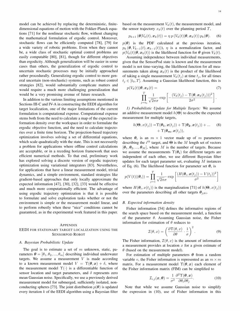
The goal is to estimate a set of m unknown, static, pa-rameters θ = [θ1, θ2, ..., θm] describing individual underwatertargets. We assume a measurement V is made accordingto a known measurement model V = Υ(θ,x) + δ, wherethe measurement model Υ(·) is a differentiable function ofsensor location and target parameters, and δ represents zeromean Gaussian noise. Specifically, we use a previously derivedmeasurement model for submerged, sufficiently isolated, non-conducting spheres [73]. The joint distribution p(θ) is updatedevery iteration k of the EEDI algorithm using a Bayesian filter

based on the measurement Vk(t), the measurement model, andthe sensor trajectory xk(t) over the planning period T ,

pk+1 (θ|Vk(t),xk(t)) = η p (Vk(t)|θ,xk(t)) pk(θ). (6)

p(θ) is the PDF calculated at the previous iteration,pk (θ, Vk−1(t),xk−1(t))), η is a normalization factor, andp(Vk(t)|θ,xk(t)) is the likelihood function for θ given Vk(t).

Assuming independence between individual measurements,given that the SensorPod state is known and the measurementmodel is not time-varying, the likelihood function for all mea-surements taken along xk(t) is the product of the likelihoodof taking a single measurement Vk(tj) at time tj , for all timestj ∈ [t0, T ]. Assuming a Gaussian likelihood function, this is

p(Vk(t)|θ,xk(t) = (7)T∏

j=t0

1√2πσ

exp

[− (Vk(tj)−Υ(θ,xk(tj)))

2

2σ2

].

1) Probabilistic Update for Multiple Targets: We assumean additive measurement model h(Θ) to describe the expectedmeasurement for multiple targets,

h(Θ, x(tj)) =Υ(θ1,x(tj)) + Υ(θ2,x(tj)) + ... (8)+ Υ(θm,x(tj)),

where θi is an m × 1 vector made up of m parametersdescribing the ith target, and Θ is the M length set of vectors[θ1,θ2, ...,θM ], where M is the number of targets. Becausewe assume the measurements Υ(θi) for different targets areindependent of each other, we use different Bayesian filterupdates for each target parameter set, evaluating M instancesof Eq. (6). The likelihood function for parameter set θi is

p(V (t)|(θi)) =

T∏j=1

1√2πσ

exp

[(H(θi,x(tj))− V (tj))

2

σ2

]where H(θi, x(tj)) is the marginalization [71] of h(Θ, x(tj))over the parameters describing all other targets θj 6=i.

B. Expected information density

Fisher information [54] defines the informative regions ofthe search space based on the measurement model, a functionof the parameter θ. Assuming Gaussian noise, the Fisherinformation for estimation of θ reduces to

I(θ, x) =

(∂Υ(θ, x)

∂θ· 1

σ

)2

. (9)

The Fisher information, I(θ, x) is the amount of informationa measurement provides at location x for a given estimate ofθ (based on the measurement model).

For estimation of multiple parameters θ from a randomvariable v, the Fisher information is represented as an m×mmatrix. For a measurement model Υ(θ,x) each element ofthe Fisher information matrix (FIM) can be simplified to

Ii,j(x,θ) =1

σ2

∂2Υ(θ,x)

∂θi∂θj. (10)

Note that while we assume Gaussian noise to simplifythe expression in (10), use of Fisher information in this

15

context does not strictly require Gaussian noise. The Fisherinformation can be calculated offline and stored based on themeasurement model which reduces the number of integrationsnecessary at each iteration.

Since the estimate of θ is represented as a probabilitydistribution function, we take the expected value of eachelement of I(x,θ) with respect to the joint distribution p(θ)to calculate the expected information matrix, Φ(x). This is anm×m matrix, where the i, jth element is

Φi,j(x) =1

σ2

∫θi

∫θj

∂2Υ(θ,x)

∂θi∂θjp(θi, θj) dθjdθi. (11)

This expression can be approximated as a discrete sum asrequired for computational efficiency.

Using the D-optimality metric [51] on the expected infor-mation matrix, the expected information density (EID) that is

EID(x) = det Φ(x). (12)

1) Expected Information Density for Multiple Targets:Since the total information is additive for independent obser-vations, we can write

I(Θ, x) = I(θ1, x) + ...+ I(θM , x), (13)

where each term is calculated as in (10).The expected information density for all parameters, for all

targets, can be calculated as the sum of the determinants of theexpected value of each term in Eq. (13), Φi(x), given the setof independent probabilities p(θi) for each set of parametersθi describing a single target,

EID(x) = η

M∑i

det Φi(x). (14)

Since the FIM is positive-semidefinite, the determinant of theFIM for each target is non-negative. Note that this is justone approach of combining the expected information fromseveral independent sources into a single map. Another optionwould have been to calculate the D-optimality for each targetindividually and calculate the subsequent trajectory based onlyon EID for the target with the highest integrated information(prior to normalization).

REFERENCES

[1] G. Mathew and I. Mezic, “Metrics for ergodicity and design of ergodicdynamics for multi-agent system,” Physica D-nonlinear Phenomena,vol. 240, no. 4-5, pp. 432–442, Feb 2011.

[2] R. Krahe and E. Fortune, “Electric fishes: neural systems, behavior andevolution,” J. Exp. Biol., vol. 13, 2013.

[3] M. E. Nelson and M. A. MacIver, “Sensory acquisition in active sensingsystems,” J. Comp. Physiol. A, vol. 192, no. 6, pp. 573–586, 2006.

[4] I. D. Neveln, Y. Bai, J. B. Snyder, J. R. Solberg, O. M. Curet, K. M.Lynch, and M. A. MacIver, “Biomimetic and bio-inspired robotics inelectric fish research,” J. Exp. Biol., vol. 216, no. Pt 13, pp. 2501–2514,Jul 2013.

[5] J. R. Solberg, K. M. Lynch, and M. A. MacIver, “Active electrolocationfor underwater target localization,” International Journal of RoboticsResearch, vol. 27, no. 5, pp. 529–548, 2008.

[6] M. A. MacIver, E. Fontaine, and J. W. Burdick, “Designing futureunderwater vehicles: principles and mechanisms of the weakly electricfish,” IEEE J. Ocean. Eng., vol. 29, no. 3, pp. 651–659, 2004.

[7] S. Cowen, S. Briest, and J. Dombrowski, “Underwater docking ofautonomous undersea vehicles using optical terminal guidance,” inMTS/IEEE OCEANS Conf., vol. 2, Oct 1997, pp. 1143–1147.

[8] C. Kreucher, K. Kastella, and A. O. Hero, “Sensor management using anactive sensing approach,” Signal Processing, vol. 85, no. 3, pp. 607–624,2005.

[9] D. Fox, W. Burgard, and S. Thrun, “Active Markov localization formobile robots,” Robotics and Autonomous Systems, vol. 25, no. 3-4, pp.195–207, 1998.

[10] C. Cai and S. Ferrari, “Information-driven sensor path planning byapproximate cell decomposition,” IEEE Transactions on Systems, Man,and Cybernetics, vol. 39, no. 3, pp. 672–689, 2009.

[11] J. Toh and S. Sukkarieh, “A Bayesian formulation for the prioritizedsearch of moving objects,” in IEEE Int. Conf. on Robotics and Automa-tion (ICRA), 2006, pp. 219–224.

[12] J. Cooper and M. Goodrich, “Towards combining UAV and sensoroperator roles in UAV-enabled visual search,” in IEEE Int. Conf. onHuman Robot Interaction (HRI), 2008, pp. 351–358.

[13] G. A. Hollinger, B. Englot, F. S. Hover, U. Mitra, and G. S. Sukhatme,“Active planning for underwater inspection and the benefit of adaptivity,”International Journal of Robotics Research, vol. 32, no. 1, pp. 3–18,2013.

[14] J. Denzler and C. Brown, “Information theoretic sensor data selectionfor active object recognition and state estimation,” IEEE Transactions onPattern Analysis and Machine Intelligence, vol. 24, no. 2, pp. 145–157,2002.

[15] T. Arbel and F. Ferrie, “Viewpoint selection by navigation throughentropy maps,” in IEEE Int. Conf. on Computer Vision, vol. 1, 1999,pp. 248–254 vol.1.

[16] Y. Ye and J. K. Tsotsos, “Sensor planning for 3D object search,”Computer Vision and Image Understanding, vol. 73, no. 2, pp. 145 –168, 1999.

[17] P.-P. Vazquez, M. Feixas, M. Sbert, and W. Heidrich, “Viewpointselection using viewpoint entropy.” in Vision Modeling and VisualizationConference, vol. 1, 2001, pp. 273–280.

[18] N. A. Massios and R. B. Fisher, “A best next view selection algorithmincorporating a quality criterion,” in British Machine Vision Conference,1998, pp. 78.1–78.10.

[19] Y. Takeuchi, N. Ohnishi, and N. Sugie, “Active vision system based oninformation theory,” Systems and Computers in Japan, vol. 29, no. 11,pp. 31–39, 1998.

[20] N. Cao, K. H. Low, and J. M. Dolan, “Multi-robot informative pathplanning for active sensing of environmental phenomena: A tale of twoalgorithms,” in International Conference on Autonomous Agents andMulti-agent Systems, 2013, pp. 7–14.

[21] A. Bender, S. B. Williams, and O. Pizarro, “Autonomous exploration oflarge-scale benthic environments,” in IEEE Int. Conf. on Robotics andAutomation (ICRA), 2013, pp. 390–396.

[22] R. Marchant and F. Ramos, “Bayesian optimisation for informative con-tinuous path planning,” in IEEE Int. Conf. on Robotics and Automation(ICRA). IEEE, 2014, pp. 6136–6143.

[23] R. Sim and N. Roy, “Global a-optimal robot exploration in SLAM,” inIEEE Int. Conf. on Robotics and Automation (ICRA), 2005, pp. 661–666.

[24] C. Leung, S. Huang, N. Kwok, and G. Dissanayake, “Planning underuncertainty using model predictive control for information gathering,”Robotics and Autonomous Systems, vol. 54, no. 11, pp. 898–910,November 2006.

[25] H. J. S. Feder, J. J. Leonard, and C. M. Smith, “Adaptive mobile robotnavigation and mapping,” International Journal of Robotics Research,vol. 18, no. 7, pp. 650–668, 1999.

[26] J. Vander Hook, P. Tokekar, and V. Isler, “Cautious greedy strategy forbearing-based active localization: Experiments and theoretical analysis,”in Robotics and Automation (ICRA), 2012 IEEE International Confer-ence on, May 2012, pp. 1787–1792.

[27] R. Marchant and F. Ramos, “Bayesian optimisation for intelligentenvironmental monitoring,” in IEEE Int. Conf. on Intelligent Robots andSystems (IROS), Oct 2012, pp. 2242–2249.

[28] E.-M. Wong, F. Bourgault, and T. Furukawa, “Multi-vehicle Bayesiansearch for multiple lost targets,” in IEEE Int. Conf. on Robotics andAutomation (ICRA), 2005, pp. 3169–3174.

[29] C. Stachniss and W. Burgard, “Exploring unknown environments withmobile robots using coverage maps,” in IJCAI, 2003, pp. 1127–1134.

[30] C. Kreucher, J. Wegrzyn, M. Beauvais, and R. Conti, “Multiplatforminformation-based sensor management: an inverted UAV demonstration,”in SPIE Defense Transformation and Network-Centric Systems, vol.6578, 2007, pp. 65 780Y–1–65 780Y–11.

[31] N. Roy and C. Earnest, “Dynamic action spaces for information gainmaximization in search and exploration,” in American Controls Conf.(ACC), June 2006, pp. 6 pp.–.

16

[32] W. Lu, G. Zhang, S. Ferrari, R. Fierro, and I. Palunko, “An informationpotential approach for tracking and surveilling multiple moving targetsusing mobile sensor agents,” in SPIE Unmanned Systems Technology,vol. 8045, 2011, pp. 80 450T–1–80 450T–13.

[33] F. Bourgault, A. A. Makarenko, S. Williams, B. Grocholsky, andH. Durrant-Whyte, “Information based adaptive robotic exploration,” inIEEE Int. Conf. on Intelligent Robots and Systems (IROS), vol. 1, 2002,pp. 540 – 545.

[34] A. Elfes, “Using occupancy grids for mobile robot perception andnavigation,” Computer, vol. 22, no. 6, pp. 46 –57, Jun 1989.

[35] A. Singh, A. Krause, C. Guestrin, and W. J. Kaiser, “Efficient informa-tive sensing using multiple robots,” In Journal of Journal of ArtificialIntelligence Research (JAIR), vol. 34, pp. 707–755, 2009.

[36] T. N. Hoang, K. H. Low, P. Jaillet, and M. Kankanhalli, “Nonmyopicε-Bayes-optimal active learning of gaussian processes,” in InternationalConference on Machine Learning, 2014, pp. 739–747.

[37] K. H. Low, J. M. Dolan, and P. Khosla, “Adaptive multi-robot wide-areaexploration and mapping,” in Conference on Autonomous agents andmultiagent systems. International Foundation for Autonomous Agentsand Multiagent Systems, 2008, pp. 23–30.

[38] J. Souza, R. Marchant, L. Ott, D. Wolf, and F. Ramos, “Bayesianoptimisation for active perception and smooth navigation,” in IEEE Int.Conf. on Robotics and Automation (ICRA), May 2014, pp. 4081–4087.

[39] R. Bajcsy, “Active perception,” Proceedings of the IEEE, vol. 76, no. 8,pp. 996–1005, 1988.

[40] J. R. Spletzer and C. J. Taylor, “Dynamic sensor planning and control foroptimally tracking targets,” International Journal of Robotics Research,vol. 22, no. 1, pp. 7–20, 2003.

[41] B. DasGupta, J. P. Hespanha, J. Riehl, and E. Sontag, “Honey-pot con-strained searching with local sensory information,” Nonlinear Analysis:Theory, Methods & Applications, vol. 65, no. 9, pp. 1773–1793, 2006.

[42] G. Zhang and S. Ferrari, “An adaptive artificial potential functionapproach for geometric sensing,” in IEEE Int. Conf. on Decision andControl (CDC), 2009, pp. 7903–7910.

[43] G. Hager and M. Mintz, “Computational methods for task-directed sen-sor data fusion and sensor planning,” International Journal of RoboticsResearch, vol. 10, no. 4, pp. 285–313, 1991.

[44] G. Benet, F. Blanes, J. Simo, and P. Perez, “Using infrared sensorsfor distance measurement in mobile robots,” Robotics and AutonomousSystems, vol. 40, no. 4, pp. 255 – 266, 2002.

[45] J. Denzler, M. Zobel, and H. Niemann, “Information theoretic focallength selection for real-time active 3d object tracking,” in IEEE Int.Conf. on Computer Vision, vol. 1, Oct 2003, pp. 400–407.

[46] J. Tisdale, Z. Kim, and J. K. Hedrick, “Autonomous UAV path planningand estimation,” IEEE Robotics and Automation Magazine, vol. 16,no. 2, pp. 35–42, June 2009.

[47] B. Grocholsky, J. Keller, V. Kumar, and G. Pappas, “Cooperative air andground surveillance,” IEEE Robotics and Automation Magazine, vol. 13,no. 3, pp. 16–25, 2006.

[48] W. Lu, G. Zhang, and S. Ferrari, “An information potential approachto integrated sensor path planning and control,” IEEE Transactions onRobotics, vol. 30, no. 4, pp. 919–934, Aug 2014.

[49] G. Zhang, S. Ferrari, and M. Qian, “An information roadmap methodfor robotic sensor path planning,” Journal of Intelligent and RoboticSystems, vol. 56, no. 1-2, pp. 69–98, 2009.

[50] X. Liao and L. Carin, “Application of the theory of optimal experimentsto adaptive electromagnetic-induction sensing of buried targets,” IEEETransactions on Pattern Analysis and Machine Intelligence, vol. 26,no. 8, pp. 961–972, 2004.

[51] A. Emery and A. V. Nenarokomov, “Optimal experiment design,”Measurement Science and Technology, vol. 9, no. 6, p. 864, 1998.

[52] D. Ucinski and J. Korbicz, “Path planning for moving sensors inparameter estimation of distributed systems,” in Workshop on RobotMotion and Control (RoMoCo), 1999, pp. 273–278.

[53] D. Ucinski, “Optimal sensor location for parameter estimation of dis-tributed processes,” International Journal of Control, vol. 73, no. 13,pp. 1235–1248, 2000.

[54] R. B. Frieden, Science from Fisher Information: A Unification. Cam-bridge University Press, 2004.

[55] N. Atanasov, B. Sankaran, J. Le Ny, G. Pappas, and K. Daniilidis,“Nonmyopic view planning for active object classification and poseestimation,” IEEE Transactions on Robotics, vol. 30, no. 5, pp. 1078–1090, Oct 2014.

[56] Y. F. Li and Z. G. Liu, “Information entropy based viewpoint planningfor 3-D object reconstruction,” IEEE Transactions on Robotics, vol. 21,no. 3, pp. 324–327, 2005.

[57] M. Rahimi, M. Hansen, W. Kaiser, G. Sukhatme, and D. Estrin,“Adaptive sampling for environmental field estimation using roboticsensors,” in IEEE Int. Conf. on Intelligent Robots and Systems (IROS),Aug 2005, pp. 3692–3698.

[58] G. A. Hollinger and G. S. Sukhatme, “Sampling-based robotic informa-tion gathering algorithms,” International Journal of Robotics Research,vol. 33, no. 9, pp. 1271–1287, 2014.

[59] A. Ryan and J. K. Hedrick, “Particle filter based information-theoreticactive sensing,” Robotics and Autonomous Systems, vol. 58, no. 5, pp.574 – 584, 2010.

[60] R. Martinez-Cantin, N. de Freitas, E. Brochu, J. Castellanos, andA. Doucet, “A Bayesian exploration-exploitation approach for optimalonline sensing and planning with a visually guided mobile robot,”Autonomous Robots, vol. 27, no. 2, pp. 93–103, 2009.

[61] H. Jacobs, S. Nair, and J. Marsden, “Multiscale surveillance of Rieman-nian manifolds,” in American Controls Conf. (ACC), 2010, pp. 5732–5737.

[62] A. D. Wilson, J. A. Schultz, and T. D. Murphey, “Trajectory synthesisfor fisher information maximization,” IEEE Transactions on Robotics,vol. 30, no. 6, 2014.

[63] D. Song, C.-Y. Kim, and J. Yi, “Simultaneous localization of multipleunknown and transient radio sources using a mobile robot,” IEEETransactions on Robotics, vol. 28, no. 3, pp. 668 –680, june 2012.

[64] C.-Y. Kim, D. Song, Y. Xu, J. Yi, and X. Wu, “Cooperative search ofmultiple unknown transient radio sources using multiple paired mobilerobots,” IEEE Transactions on Robotics, vol. 30, no. 5, pp. 1161–1173,Oct 2014.

[65] L.M. Miller and T.D. Murphey, “Trajectory optimization for continuousergodic exploration,” in American Controls Conf. (ACC), 2013, pp.4196–4201.

[66] L. M. Miller and T. D. Murphey, “Trajectory optimization for continuousergodic exploration on the motion group SE(2),” in IEEE Int. Conf. onDecision and Control (CDC), 2013, p. In Press.

[67] E. Acar, H. Choset, Y. Zhang, and M. Schervish, “Path planning forrobotic demining: Robust sensor-based coverage of unstructured envi-ronments and probabilistic methods,” International Journal of RoboticsResearch, vol. 22, no. 7 - 8, pp. 441 – 466, July 2003.

[68] H. Choset, “Coverage for robotics–a survey of recent results,” Annalsof mathematics and artificial intelligence, vol. 31, no. 1-4, pp. 113–126,2001.

[69] A. Krause and C. Guestrin, “Nonmyopic active learning of gaussianprocesses: an exploration-exploitation approach,” in International Con-ference on Machine learning. ACM, 2007, pp. 449–456.

[70] J. Hauser, “A projection operator approach to the optimization oftrajectory functionals,” in IFAC world congress, vol. 4, 2002, pp. 3428–3434.

[71] G. S. Chirikjian, Stochastic Models, Information Theory, and LieGroups, Volume 1: Classical Results and Geometric Methods. SpringerScience & Business Media, 2009.

[72] G. S. Chirikjian and A. B. Kyatkin, Engineering Applications of Non-commutative Harmonic Analysis. CRC Press, 2000.

[73] Y. Bai, J. B. Snyder, M. Peshkin, and M. A. MacIver, “Findingand identifying simple objects underwater with active electrosense,”International Journal of Robotics Research, vol. 1, no. 23, 2015.

[74] S. Thrun, “Learning occupancy grid maps with forward sensor models,”Autonomous Robots, vol. 15, no. 2, pp. 111–127, 2003.

[75] S. Thrun, W. Burgard, and D. Fox, Probabilistic Robotics. Cambridge,Mass: The MIT Press, 2005.

[76] Y. Silverman, L. M. Miller, M. A. MacIver, and T. D. Murphey, “Optimalplanning for information acquisition,” in IEEE Int. Conf. on IntelligentRobots and Systems (IROS), vol. 5974- 5980, 2013.

[77] M. E. Nelson and M. A. MacIver, “Sensory acquisition in active sensingsystems,” Journal of Comparative Physiology A, vol. 192, no. 6, pp.573–586, 2006.

[78] Y. Zhou and G. S. Chirikjian, “Probabilistic models of dead-reckoningerror in nonholonomic mobile robots,” in IEEE Int. Conf. on Roboticsand Automation (ICRA), vol. 2, 2003, pp. 1594–1599.

[79] Y. Wang and G. Chirikjian, “A diffusion-based algorithm for workspacegeneration of highly articulated manipulators,” in IEEE Int. Conf. onRobotics and Automation (ICRA), vol. 2, 2002, pp. 1525–1530 vol.2.

[80] E. Todorov and W. Li, “A generalized iterative lqg method for locally-optimal feedback control of constrained nonlinear stochastic systems,”in American Controls Conf. (ACC), 2005, pp. 300–306.

[81] M. B. Horowitz and J. W. Burdick, “Semidefinite relaxations forstochastic optimal control policies,” in American Controls Conf. (ACC),2014, pp. 3006–3012.

17

[82] K. Zhou and J. C. Doyle, Essentials of robust control. Prentice hallUpper Saddle River, NJ, 1998, vol. 180.

[83] A. Prabhakar, K. Flaßkamp, and T. Murphey, “Time discretization inoptimal ergodic control,” in IEEE Int. Conf. on Decision and Control(CDC), 2015.