erdc/tn smart-04-3, description of the hydrologic ... · erdc/tn smart-04-3 september 2004 1...

ERDC/TN SMART-04-3 September 2004

1

Description of the Hydrologic Engineering Center’s Hydrologic

Modeling System (HEC-HMS) and Application to Watershed Studies

by Matt Fleming

PURPOSE: The objective of this document is to describe the Hydrologic Engineering Center’s Hydrologic Modeling System (HEC-HMS) program and its application to watershed studies. HMS has the capability to serve as a cornerstone program with respect to the watershed perspective approach. HMS can simulate the rainfall-runoff at any point within a watershed given physical characteristics of the watershed. It is a tool for watershed management in that an HMS model can be developed to account for human impact to determine the effect on the magnitude, quantity, and timing of runoff at points of interest. Results from an HMS model can be used by a number of other programs to determine impact in areas such as water quality and flood damage. MODEL DESCRIPTION Overview. The Hydrologic Modeling System is designed to simulate the precipitation-runoff processes of dendritic watershed systems. It is applicable in a wide range of geographic areas for solving the widest possible range of problems. This includes large river basin water supply and flood hydrology, and small urban or natural watershed runoff. Hydrographs produced by the program are used directly or in conjunction with other software for studies of water availability, urban drainage, flow forecasting, future urbanization impact, reservoir spillway design, flood damage reduction, floodplain regulation, wetlands hydrology, and systems operation. HMS features a completely integrated work environment including a database, data entry utilities, computation engine, and results reporting tools. A graphical user interface allows the user seamless movement between the different parts of the program. Program functionality and appearance are the same across all supported platforms. Time-series, paired, and gridded data are stored in the Data Storage System HEC-DSS (U.S. Army Corps of Engineers (USACE) 2003). Storage and retrieval of data are handled by the program and are generally transparent to the user. Precipitation and discharge gauge information can be entered manually within the program or can be loaded from previously created DSS files. Results stored by the program in the database are accessible by other HEC software. Data entry can be performed for individual basin elements such as subbasins and stream reaches or simultaneously for entire classes of similar elements. Tables and forms for entering necessary data are accessed from a visual schematic of the basin. All computations are performed in metric units. Input data and output results may be U.S. customary or metric and are automatically converted when necessary.

Report Documentation Page Form ApprovedOMB No. 0704-0188

Public reporting burden for the collection of information is estimated to average 1 hour per response, including the time for reviewing instructions, searching existing data sources, gathering andmaintaining the data needed, and completing and reviewing the collection of information. Send comments regarding this burden estimate or any other aspect of this collection of information,including suggestions for reducing this burden, to Washington Headquarters Services, Directorate for Information Operations and Reports, 1215 Jefferson Davis Highway, Suite 1204, ArlingtonVA 22202-4302. Respondents should be aware that notwithstanding any other provision of law, no person shall be subject to a penalty for failing to comply with a collection of information if itdoes not display a currently valid OMB control number.

1. REPORT DATE SEP 2004 2. REPORT TYPE

3. DATES COVERED -

4. TITLE AND SUBTITLE Description of the Hydrologic Engineering Center’s Hydrologic ModelingSysem (HEC-HMS) and Application to Watershed Studies

5a. CONTRACT NUMBER

5b. GRANT NUMBER

5c. PROGRAM ELEMENT NUMBER

6. AUTHOR(S) 5d. PROJECT NUMBER

5e. TASK NUMBER

5f. WORK UNIT NUMBER

7. PERFORMING ORGANIZATION NAME(S) AND ADDRESS(ES) Army Engineer Research and Development Center,EnvironmentalLaboratory,3909 Halls Ferry Road,Vicksburg,MS,39180-6199

8. PERFORMING ORGANIZATIONREPORT NUMBER

9. SPONSORING/MONITORING AGENCY NAME(S) AND ADDRESS(ES) 10. SPONSOR/MONITOR’S ACRONYM(S)

11. SPONSOR/MONITOR’S REPORT NUMBER(S)

12. DISTRIBUTION/AVAILABILITY STATEMENT Approved for public release; distribution unlimited

13. SUPPLEMENTARY NOTES The original document contains color images.

14. ABSTRACT see report

15. SUBJECT TERMS

16. SECURITY CLASSIFICATION OF: 17. LIMITATION OF ABSTRACT

18. NUMBEROF PAGES

17

19a. NAME OFRESPONSIBLE PERSON

a. REPORT unclassified

b. ABSTRACT unclassified

c. THIS PAGE unclassified

Standard Form 298 (Rev. 8-98) Prescribed by ANSI Std Z39-18


2

History. The computation engine draws on over 30 years experience with hydrologic simulation software. Many algorithms from HEC-1 (USACE 1998), HEC-1F (USACE 1989), PRECIP (USACE 1989), and HEC-IFH (USACE 1992) have been modernized and combined with new algorithms to form a comprehensive library of simulation routines. The current research program is designed to produce new algorithms and analysis techniques for addressing emerging problems. The program is comprised of a graphical user interface, integrated hydrologic analysis components, data storage and management tools, and graphics and reporting facilities. Development utilized a mixture of programming languages including C, C++, and FORTRAN. The computation engine and graphical user interface are written in object-oriented C++. Hydrologic process algorithms are written in FORTRAN and have been organized into the libHydro library. Data are managed using the HecLib library. The program was and is developed by the United States Federal Government at taxpayer expense and is therefore in the public domain. A team of HEC staff and consultants developed the program under the HEC "Next Generation Software Development Project" led by the Director, Darryl Davis. Arlen Feldman, Chief of the Hydrology and Hydraulics Technology Division, managed the general design, development, testing, and documentation of the program. Version 2.2.2 should be the terminal release using the C++ programming language and the Galaxy library. All future releases, beginning with Version 3.0, will be developed using the Java language. The existing interface was replaced with one written in Java that compares nicely with other engineering and scientific software programs from commercial companies. Version 3.0 will contain all of the capability present in Version 2.2.2 and will also add snowmelt simulation to the meteorologic model. Algorithms originally developed for the Distributed Snow Process Model (DSPM) are being adapted for use in HEC-HMS. As time allows, features in addition to snowmelt simulation will be added to HMS. These features may include customizable reports, automatic depth-area reduction analysis, additional reservoir capabilities for modeling interior flood zones, energy budget snowmelt simulation, user scripting to automate simple tasks, frequency curve generation, and internationalization of the software. Work is under way to implement the new design for the interface, and an approximate date for the beta release of Version 3.0 is winter 2004. General Description. When developing an HMS model, a Basin Model, Metrological Model, and Control Specifications need to be defined (Figure 1). The physical representation of watersheds or basins and rivers is configured in the basin model. Hydrologic elements are connected in a dendritic network to simulate runoff processes. Available elements are: subbasin, reach, junction, reservoir, diversion, source, and sink. Meteorologic data analysis is performed by the meteorologic model and includes precipitation and evapotranspiration. The time span of a simulation is controlled by control specifications, which include a starting date and time, ending date and time, and computation time step. Hydrologic elements are the building blocks of a basin model. Figure 2 shows the “Castro 1” basin model from Figure 1. There are four subbasin elements, two reach elements, and three junction elements in the basin model. Each element represents part of the total response of the watershed to precipitation. Table 1 lists and provides a description for each element available in a basin model. An element uses a mathematical model to describe the physical process.


3

Figure 1. Example HMS model. The name of the model is “Castro.” In this

HMS model there are two basin models, “Castro 1” and “Castro 2,” one meteorologic model “GageWts,” and one control specification, “Jan 73”

Figure 2. Basin model elements in the “Castro 1” basin model


4

Table 1 Description of Basin Model Element Element Description

Subbasin A subbasin is an element that usually has no inflow and only one outflow. This element is one of only two ways to produce flow in the basin model. Outflow is computed from meteorologic data by subtracting losses, transforming excess precipitation, and adding baseflow. The subbasin can be used to model a wide range of watershed catchment sizes.

Reach A reach is an element with one or more inflows and only one outflow. Inflow comes from other elements in the basin model. If there is more than one inflow, all inflows are added together before computing the outflow. Outflow is computed using one of the several available methods for simulating open channel flow. The reach can be used to model rivers and streams.

Reservoir A reservoir is an element with one or more inflows and one computed outflow. Inflow comes from other elements in the basin model. If there is more than one inflow, all inflows are added together before computing the outflow. Assuming that the water surface is level, outflow is either computed using a user-specified monotonically increasing storage-outflow relationship or an outlet structure and an elevation-storage relationship. The element can be used to model reservoirs, lakes, and ponds.

Junction A junction is an element with one or more inflows and only one outflow. All inflow is added together to produce the outflow by assuming zero storage at the junction. It is usually used to represent a river or stream confluence.

Diversion A diversion is an element with two outflows, main and diverted, and one or more inflows. Inflow comes from other elements in the basin model. If there is more than one inflow, all inflows are added together before computing the outflows. The amount of diverted outflow is computed from a user-specified monotonically increasing inflow-diversion relationship. Diverted outflow can be connected to an element that is computationally downstream. The diversion can be used to represent weirs that divert flow into canals, flumes, or off-stream storage.

Source A source is an element with no inflow, one outflow, and is one of only two ways to produce flow in the basin model. The source can be used to represent boundary conditions to the basin model such as measured outflow from reservoirs or unmodeled headwater regions.

Sink A sink is an element with one or more inflows but no outflow. Multiple inflows are added together to determine the total amount of water entering the element. Sinks can be used to represent the lowest point of an interior drainage area or the outlet of the basin model.

Sometimes the model is only a good approximation of the original physical process over a limited range of environmental conditions. As noted above, a mathematical model consists of equations that represent the behavior of various hydrologic system components. Herein the term method is used in this context. For example, the Muskingum-Cunge channel routing method encapsulates equations for continuity and momentum to form a mathematical model of open-channel flow for routing. All of the details of the equations, initial conditions, state variables, boundary conditions, and method of solving the equations are contained within the method. To make the program suitable for many different conditions, most elements have more than one method for approximating the physical process. For example, there are seven different methods for calculating the excess precipitation in a subbasin element. Table 2 lists available methods for certain basin model elements and the precipitation model. The program provides the following methods:


5

Table 2 Summary of Simulation Methods Included in HEC-HMS Category Method

User-specified hyetograph User-specified gauge weighting Inverse-distance-squared gauge weighting Gridded precipitation Frequency-based hypothetical storms Standard project storm (SPS) for eastern U.S.

Precipitation

Soil conservation service (SCS) hypothetical storm Evapotranspiration Monthly average

Initial and constant rate SCS curve number (CN) Gridded SCS CN Green and Ampt Deficit and constant rate Soil moisture accounting (SMA)

Loss

Gridded SMA User-specified unit hydrograph (UH) Clark’s UH Snyder’s UH SCS UH ModClark Kinematic wave

Direct runoff

User-specified s-graph Constant monthly Exponential recession

Baseflow

Linear reservoir Kinematic wave Lag Modified Puls Muskingum Muskingum-Cunge standard section Muskingum-Cunge 8-point section Diversion

Routing

Reservoir

• Precipitation methods: describe an observed (historical) precipitation event, a frequency-

based hypothetical precipitation event, or an event that represents the upper limit of precipitation possible at a given location. Also, a snowmelt method is being added that can partition precipitation into rainfall and snowfall and then account for accumulation and melt


6

of the snowpack. These methods describe the spatial and temporal distribution of precipitation on a watershed.

• Evapotranspiration methods: used in continuous simulation for computing the amount of

water that is removed back to the atmosphere through evaporation and plant use. • Loss methods: estimate the amount of precipitation that infiltrates from the land surface into

the soil. Among the loss methods are a simple one-layer and more complex five-layer soil-moisture-accounting model for continuous simulation. They can be used to simulate the long-term response of a watershed to wetting and drying. The loss methods address questions about the volume of precipitation that falls on the watershed: How much infiltrates on pervious surfaces? How much runs off of the impervious surfaces? When does it run off?

• Direct-runoff methods: describe overland flow, storage, and energy losses as water runs off a

watershed and into the stream channels. These are generally called transform methods because they "transform" excess precipitation into watershed outflow. These methods describe what happens as water that has not infiltrated or been stored on the watershed moves over or just beneath the watershed surface. A quasi-distributed transform model for use with distributed precipitation data, such as the data available from radar, is available.

• Baseflow methods: estimate the amount of infiltrated water returning to the channel. Some

of the included methods conserve mass through the infiltration process to baseflow; others do not have the same conserving properties. These methods simulate the slow subsurface drainage of water from a hydrologic system into the watershed’s channels.

• Hydrologic routing methods: account for storage and energy flux as water moves through

stream channels and water control structures. These routing methods simulate one-dimensional open channel flow, thus predicting time series of flow, stage, or velocity, given upstream hydrographs.

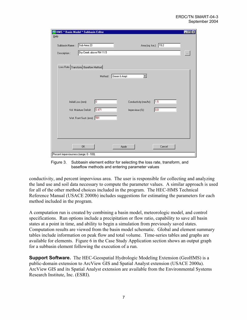
The program has been designed to be as flexible as possible in defining the hydrologic system. For example, the user could choose to combine the deficit and constant rate loss method with the Clark transform method. The program will do the work of connecting the excess precipitation from the loss method to the transform method for computing surface runoff. Most methods can be successfully combined with any other method to compute watershed discharge. However, the applicability of any particular method depends on the characteristics of the watershed and some methods may not be appropriate for some hydrologic engineering studies. The data-entry steps, program execution, and result visualization are easy with the HMS program. Each of the subbasin model elements and the precipitation model have an editor for selecting computation methods and entering the required parameter data. The user indicates method choices and specifies initial conditions and parameters using a graphical user interface (GUI). Figure 3 is an example of the subbasin element editor in the basin model. Notice that the Green and Ampt loss rate method is selected and the required parameters are shown. In general, the user enters quantitative parameter values. For example, the Green and Ampt infiltration method requires an initial loss, volume moisture deficit, wetting front suction, hydraulic


7

Figure 3. Subbasin element editor for selecting the loss rate, transform, and

baseflow methods and entering parameter values conductivity, and percent impervious area. The user is responsible for collecting and analyzing the land use and soil data necessary to compute the parameter values. A similar approach is used for all of the other method choices included in the program. The HEC-HMS Technical Reference Manual (USACE 2000b) includes suggestions for estimating the parameters for each method included in the program. A computation run is created by combining a basin model, meteorologic model, and control specifications. Run options include a precipitation or flow ratio, capability to save all basin states at a point in time, and ability to begin a simulation from previously saved states. Computation results are viewed from the basin model schematic. Global and element summary tables include information on peak flow and total volume. Time-series tables and graphs are available for elements. Figure 6 in the Case Study Application section shows an output graph for a subbasin element following the execution of a run. Support Software. The HEC-Geospatial Hydrologic Modeling Extension (GeoHMS) is a public-domain extension to ArcView GIS and Spatial Analyst extension (USACE 2000a). ArcView GIS and its Spatial Analyst extension are available from the Environmental Systems Research Institute, Inc. (ESRI).


8

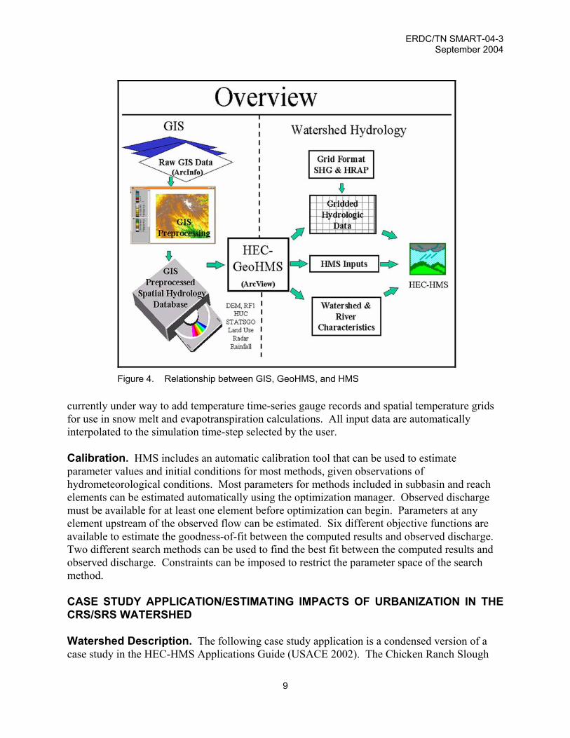
HEC-GeoHMS has been developed as a geospatial hydrology tool kit for engineers and hydrologists with limited GIS experience. The program allows users to visualize spatial information, document watershed characteristics, perform spatial analysis, delineate subbasins and streams, construct inputs to hydrologic models, and assist with report preparation. Working with HEC-GeoHMS through its interfaces, menus, tools, buttons, and context-sensitive online help, in a Windows environment, allows the user to expediently create hydrologic inputs that can be used directly with the HEC-HMS program. The current version of HEC-GeoHMS creates a background map file, lumped basin model, a grid-cell parameter file, and a distributed basin model. The background map file contains the stream alignments and subbasin boundaries. The lumped basin model contains hydrologic elements and their connectivity to represent the movement of water through the drainage system. To assist with estimating hydrologic parameters, tables containing physical characteristics of streams and watersheds can be generated. If the hydrologic model employs the distributive techniques for hydrograph transformation, i.e. ModClark, and grid-based precipitation, then a grid-cell parameter file and a distributed basin model at the grid-cell level can be generated. The relationship between GIS, HEC-GeoHMS, and HEC-HMS is illustrated in Figure 4. The GIS capability is used for heavy data formatting, processing, and coordinate transformation. The end result of the GIS processing is a spatial hydrology database that consists of the digital elevation model (DEM), soil types, land use information, rainfall, etc. Currently, HEC-GeoHMS operates on the DEM to derive subbasin delineation and prepare a number of hydrologic inputs. HEC-HMS accepts these hydrologic inputs as a starting point for hydrologic modeling. With the vertical dashed line separating the roles of the GIS and the watershed hydrology, HEC-GeoHMS provides the connection for translating GIS spatial information into hydrologic models. Model Development. The HEC-HMS Applications Guide (USACE 2002) lists the following steps that can be taken to obtain the desired result using the HMS program:

1. Identify the decision required. 2. Determine what information is required to make a decision. 3. Determine the appropriate spatial and temporal extent of information required. 4. Identify methods that can provide the information, identify criteria for selecting one of the

methods, and select a method. 5. Calibrate and verify the model. 6. Collect/develop boundary conditions and initial conditions appropriate for the application. 7. Apply the model. 8. Do a reality check and analyze sensitivity. 9. Process results to derive required information.

Input data requirements depend on the method choices made by the user. Precipitation data are required for almost all applications and are subsequently processed within the program to produce a precipitation boundary condition for the watershed. Depending on the use, precipitation data may be time-series gauge records, spatial grids from radar rainfall estimates, or statistical data from a NOAA product such as TP-40. Discharge records may be required as an upstream boundary condition when only part of a watershed is modeled. Development is


9

Figure 4. Relationship between GIS, GeoHMS, and HMS

currently under way to add temperature time-series gauge records and spatial temperature grids for use in snow melt and evapotranspiration calculations. All input data are automatically interpolated to the simulation time-step selected by the user. Calibration. HMS includes an automatic calibration tool that can be used to estimate parameter values and initial conditions for most methods, given observations of hydrometeorological conditions. Most parameters for methods included in subbasin and reach elements can be estimated automatically using the optimization manager. Observed discharge must be available for at least one element before optimization can begin. Parameters at any element upstream of the observed flow can be estimated. Six different objective functions are available to estimate the goodness-of-fit between the computed results and observed discharge. Two different search methods can be used to find the best fit between the computed results and observed discharge. Constraints can be imposed to restrict the parameter space of the search method. CASE STUDY APPLICATION/ESTIMATING IMPACTS OF URBANIZATION IN THE CRS/SRS WATERSHED Watershed Description. The following case study application is a condensed version of a case study in the HEC-HMS Applications Guide (USACE 2002). The Chicken Ranch Slough


10

and Strong Ranch Slough (CRS/SRS) watershed is an urban watershed of approximately 15 square miles within Sacramento County, in northern California. The watershed and surrounding area are shown in Figure 5. The Strong Ranch Slough and Sierra Branch portion of the watershed is 7.1 square miles and the Chicken Ranch Slough portion is approximately 6.8 square miles. The watershed is developed primarily for residential, commercial, and public uses. The terrain in the watershed is relatively flat. The soil is primarily of sandy loam. It exhibits a high runoff potential.

Figure 5. Chicken Ranch Slough and Strong Ranch Slough watersheds

Located in the headwaters of CRS is a 320-acre (0.5-square-mile) undeveloped area. As a result of increasing land values, the owners of the land are petitioning to rezone their land and develop it for new homes and businesses. In order for development to be allowed, the owners must mitigate for any increased runoff caused by the development. In this case, that requirement is imposed by the local authorities. However, a similar requirement is commonly included as a component of the local cooperation agreement for Federally funded flood-damage-reduction projects. This ensures that future development in a watershed be limited so the protection provided by the project is not compromised. This requirement is especially important in the CRS/SRS watershed because there is already a flood risk near the outlet of the watershed. In the feasibility phase of the project, the following questions need to be answered:

1. Will the development of the open area increase the peak runoff in the Chicken Ranch Slough watershed for the 0.01 annual exceedance probability (AEP) event?

2. If so, how significant is the increase in flow, volume, and peak stage?


11

Information Required. To answer the questions above, the following information is required:

• The without-development peak runoff for the selected event. • The with-development peak runoff for the selected event.

To provide that information, the HMS Program will use a watershed model to compute the peak flow for the different watershed conditions. To develop the rainfall-runoff relationship, information on the watershed will need to be collected, such as:

• Soil types and infiltration rates. • Land use characteristics and the percent of impervious area due to development. • Physical characteristics of the watershed including lengths and slopes. • Local precipitation patterns. • Drainage patterns of the study area. • Drainage channel geometry and conditions.

For this study, the information required was found using results of previous drainage studies in the area, USGS topographic and soils maps, and field investigations. Spatial and Temporal Extent. The study team is interested in evaluating the increase in runoff from Chicken Ranch Slough (CRS) only. So, the portion of the watershed that contributes flow to Strong Ranch Slough will not be analyzed in this phase of the study. In the reconnaissance phase, the study team identified the portion of the CRS watershed downstream of Arden Way as being influenced by backwater from the D05 pond. The flow in this lower portion of the watershed is a function of both the channel flow and downstream channel stage. So, this lower portion will also not be included in this phase of the study. Therefore, the study area for this phase will be the portion of the watershed that contributes flow to CRS upstream of Arden Way. Now that the study area has been defined, the next step is to use the information collected to divide the study area into subbasins. By doing so, the analyst will be able to compute the flow at critical locations along CRS. To delineate the subbasins and measure the physical parameters of the watershed, the USGS quadrangle map (1:24000 scale) of the watershed was used. Method Selection. Once the watershed data were collected and the spatial and temporal extents had been determined, the analyst began constructing the HEC-HMS model. As shown in Table 2, several methods are available for runoff volume, direct runoff, and channel routing. In all cases, two or more of the methods would work for this analysis. Infiltration. The analyst chose the initial and constant rate runoff-volume method. It is widely used in the Sacramento area. Regional studies have been conducted for estimating the constant loss rate. The studies, based upon calibration of models of gauged watersheds, have related loss rates to soil type and land use. Surveys of development in the region provide estimates of percent of directly impervious area as functions of land use. Table 3 lists the estimates of percent of directly connected impervious area for CRS watershed.


12

Direct-runoff transform. The analyst used Snyder’s unit hydrograph direct-runoff transform method. This method is widely used in the Sacramento area. As with the loss method, regression studies have been conducted in Sacramento to estimate the lag of watersheds as a function of watershed properties. The lag was estimated; values are shown in Table 3.

Table 3 Unit Hydrograph Lag and Percent Impervious Estimates

Description Identifier Estimated Lag (hr)

Percent Directly Impervious

CRS u/s of Corabel gauge COR 1.78 50 CRS d/s of Corabel gauge, u/s of Fulton FUL 0.22 60 CRS d/s of Fulton, u/s of Arden Way ARD 0.75 50

Because the headwater basin is gauged, calibration can be used to estimate the Snyder peaking coefficient Cp. During the calibration process, the lag estimate can be refined as well. Baseflow. Baseflow was not included in this analysis. It is not critical in most urban watersheds. Routing. The analyst used the Muskingum-Cunge 8-point channel routing method because channel geometry and roughness values were available from previous studies. A primary advantage of the method is that it is physically based, which is useful because downstream data are not available for calibration. If the study area was defined such that it extended to the D05 pond, the modified Puls model would have been used to model the portion of the CRS channel influenced by backwater from the pond. Temporal Resolution. The analyst needed to decide upon a temporal resolution for the analysis. Decisions required include selection of the time-step to use and the hypothetical precipitation event duration. In earlier watershed programs, the selection of the time-step required was more critical due to array limitations and program computation time. These considerations are no longer needed when using HEC-HMS on a modern computer for a short duration storm. The analyst could use a 1-min time-step; however, this may provide unnecessary resolution. Model Calibration and Verification. Based upon the methods selected, the following parameters are required:

• Initial and constant loss rates and percent directly connected impervious area for the runoff-volume method.

• Lag time and peaking coefficient for the runoff transform. • Roughness values for the channel routing method.

In addition, channel properties such as reach length, energy slope, and channel geometry need to be measured for the channel routing method. The lag time and percent impervious were estimated as described above. The initial loss, constant loss rate, and peaking coefficient were


13

estimated using calibration. The initial estimate for the constant loss rate was based upon regional relationships. It was 0.07 in./hour. Because the watershed is developed and has a high percent of impervious area, the runoff hydrograph is expected to rise and fall over a short period of time. As an initial estimate for the peaking coefficient, the upper limit suggested by the HEC-HMS Technical Reference Manual (USACE 2000b) of 0.8 was used. The magnitude and AEP of historical events used for calibration should be consistent with the intended application of the model. Three significant events have occurred since the installation of the gauges in the CRS/SRS watershed. The events are:

• January 10, 1995. This is about a 0.04- to 0.01-AEP event. • January 22, 1997. This is about a 0.10- to 0.04-AEP event. • January 26, 1997. This is about a 0.20- to 0.04-AEP event.

The first two events were used to refine the parameter values using the optimization tool and the third was used to verify the final values. The calibration hydrograph for the January 22, 1997 event is shown in Figure 6. This plot shows that the computed hydrograph matches well with the observed flows for that event, especially the peak flows.

Figure 7. Calibration results for the January 22, 1997 event

The parameter estimates resulting from the calibration to the January 10, 1995 event and the January 22, 1997 event are summarized in Table 4. The values were averaged and verified using the observed precipitation and flow data for the January 26, 1997 event. The results from the


14

verification process show that the rising limb of the observed data occurs earlier than the rising limb of the computed data; the analyst reasoned that the Snyder lag value may be too great. The lag value was optimized for the January 26, 1997 event. HEC-HMS computed a value of 4.55 hr, which was similar to the parameter value computed for the January 22, 1997 event.

Table 4 Parameter Estimates from Calibration for the Headwater Basin Calibration Event Snyder Lag (hr) Snyder Cp

January 10, 1995 5.42 0.68 January 22, 1997 4.68 1.00 January 26, 1997 4.55 1.00

Final average value 4.88 0.89

The average parameter estimates from the first two events did not compare well with the third event. Consequently, the analyst averaged the parameter values from all three events. By doing so, all three events are incorporated into the calibration of the model parameters. This provided the estimates shown in Table 4. The averages of the three values were used to represent the existing condition. However, the analyst may have chosen not to weight the parameter values evenly. Based on the quality of precipitation data, magnitude of the event, or other factors, more weight may be given to a particular historical event. The Snyder lag values for subbasins FUL and ARD were adjusted from the values predicted with the regression equation consistent with the calibration. The logic followed is that the regression equation, when compared to the calibration results, under-predicts the lag for subbasins in the CRS watershed. By adjusting the parameters, the analyst fits the equation to basins found in this watershed. The peaking coefficient Cp is usually taken as a regional value. As the subbasins are similar in slope and land use, the calibrated value was used for the other two subbasins. The channel properties and parameter values needed for the Muskingum-Cunge 8-point routing method must be defined also. The reach length, energy slope, and cross-section geometry were estimated from available maps and survey data. The Manning’s roughness parameter was estimated using published tables of values (Barnes 1967). The Manning’s roughness value could be refined through calibration if reliable gauge data were available. There is a downstream gauge at Arden Way. However, due to the backwater conditions from the D05 pond, the assumption of a single relationship between stage and flow is not appropriate. Further, the observed stages at the gauge are influenced by a variety of other downstream factors such as pump operation and commingled water from SRS. Application. Once the without-development condition parameters were established, the analyst was ready to complete the HEC-HMS input and produce the information needed for decision-making. To compare land use conditions, the analyst used the 0.01 annual exceedance probability (AEP) storm event to estimate the 0.01 AEP flood. This is a standard procedure often used by the local authorities for evaluating land use changes.


15

The initial loss values estimated during calibration were storm-specific. The initial loss values used for hypothetical events are based upon studies in the Sacramento area. Adding the routing reaches and ungauged subbasins, as shown in Figure 7, completed the input.

Figure 7. CRS basin schematic

In order to complete the meteorologic model for the 0.01-AEP event, the analyst used depths from locally developed depth-duration-frequency (DDF) functions. The DDF functions are based upon data from an NWS gauge with a long period of record. Once completed, the analyst exercised the model and calculated the combined outflow hydrograph at Arden Way for the 0.01-AEP event. The resulting peak flow and total runoff volume are included in Table 5.

Table 5 HEC-HMS Results at Arden Way for 0.01 AEP Event Condition Peak Flow (cfs) Runoff Volume (ac-ft)

Existing (without development) 941 794.2 Future (with development) 1,003 828.8

Percent increase 6.6% 4.4%

To account for the development of the open area in the COR subbasin, the analyst modified the percent of impervious area, unit hydrograph, and loss rate parameters. Based on current and proposed land uses, the analyst estimated that the impervious area for the entire subbasin would


16

increase from 50 to 55 percent. Intuitively, the analyst expected that the unit hydrograph lag would decrease and the peaking coefficient Cp would increase. Using relationships from the Denver lag equation (EMSI), an increase from 50 to 55 percent impervious area would increase the Cp value by 8 percent. This results in a modified value of 0.96 for the COR subbasin. Using the regional lag equation, an increase of 5 percent of impervious area decreases the lag by 4 percent. This results in a modified lag of 4.68 hr. The loss rates are a function of the soil type. The soil type will not change with the development. So, the loss values will not change. A duplicate basin model was created, and the percent impervious, Snyder’s unit hydrograph lag, and Snyder’s Cp were modified. Using the same boundary and initial conditions as the existing condition input, the future peak flow was calculated. The resulting peak flow and total runoff volumes are summarized in Table 5. Sensitivity Analysis. The model results should be verified to determine that they agree reasonably well with related analyses and with expected results. Independent data sources and parameter values from HEC-HMS input should be used for an unbiased comparison. Alternatives include comparison to other regional studies, regional estimates of flow per unit area, nearby gauge statistics, and the USGS regional regression equations. To determine how significant this increase in flow is to the peak stage in Chicken Ranch Slough, a channel model can be used to compute stage. To do so, the analyst could use the runoff hydrograph from the HEC-HMS model as input to the HEC-River Analysis System (RAS) computer program. Using channel geometry and roughness data, the HEC-RAS Program computes water surface elevations based upon the flow input. Application Summary. The goal of this case study application was to identify whether the development of an open area in the Chicken Ranch Slough watershed increased runoff, and if so, how much. Using available watershed data and computer program HEC-HMS, the analyst was able to answer the questions. As shown in Table 5, the development does increase the peak runoff and total volume of runoff. If the development is to be permitted, some water control features must be included to reduce the peak for the 0.01 AEP storm from 1,003 cfs to 941 cfs. SUMMARY: The HMS Program is a valuable tool for predicting and managing human impact on the rainfall-runoff response at points of interest within a watershed. Results from the program can be used directly or in conjunction with other software for studies of water availability, urban drainage, flow forecasting, future urbanization impact, reservoir spillway design, flood damage reduction, floodplain regulation, wetlands hydrology, and systems operation. The following reference manuals are available from the HEC Website, www.hec.usace.army.mil, for a more in-depth description and application of the HMS program. The Hydrologic Modeling System HEC-HMS: User's Manual contains extensive information on installing and using the program. An example application is included to illustrate the steps necessary to produce results (USACE 2001). The Hydrologic Modeling System HEC-HMS: Technical Reference Manual contains information on how to use the various methods included in the program. The scientific origin and equation


17

derivations are presented for each method. Specific solution algorithms for a method are discussed when necessary for a complete understanding. Application and parameter estimation for each method is also included (USACE 2000b). The Hydrologic Modeling System HEC-HMS: Applications Guide illustrates application of program HEC-HMS to studies typical of those undertaken by Corps offices, including (1) urban flooding studies, (2) flood-frequency studies, (3) flood-loss reduction studies, (4) flood-warning system planning studies, (5) reservoir design studies, and (6) environmental studies. The online help system within the program contains topics describing each screen of the graphical user interface (USACE 2002). POINTS OF CONTACT: For additional information, contact Matt Flemming (530-756-1104, [email protected]) or Bill Scharffenberg (William.A.Scharffenberg@ usace.army.mil) or the Manager of the System-Wide Modeling, Assessment, and Restoration Technologies (SMART) Program, Dr. Steve Ashby (601-634-2387, Steven.L.Ashby@erdc. usace.army.mil). This technical note should be cited as follows:

Fleming, M. (2004). “Description of the Hydrologic Engineering Center’s Hydrologic Modeling System (HEC-HMS) and application of watershed studies,” Smart Technical Notes Collection, ERDC/TN SMART-04-3, U.S. Army Engineer Research and Development Center, Vicksburg, MS.

REFERENCES Barnes, H.H. (1967). “Roughness characteristics of natural channels,” Water-Supply Paper 1849. U.S. Geological

Survey, Washington, DC.

Environmental Modeling Systems, Incorporated. (http://www.ems-i.com/wmshelp/WMSHELP.htm) WMS Help, Denver Lag Time Equation. San Jordan, UT.

U.S. Army Corps of Engineers. (1989). “Water Control Software: Forecast and Operations,” Hydrologic Engineering Center, Davis, CA.

U.S. Army Corps of Engineers. (1992). “HEC-IFH Interior Flood Hydrology Package: User's Manual,” Hydrologic Engineering Center, Davis, CA.

U.S. Army Corps of Engineers. (1998). “HEC-1 Flood Hydrograph Package: User's Manual,” Hydrologic Engineering Center, Davis, CA.

U.S. Army Corps of Engineers. (2000a). “Geospatial Hydrologic Modeling Extension: GeoHMS,” Hydrologic Engineering Center, Davis, CA.

U.S. Army Corps of Engineers. (2000b). “HEC-HMS Technical Reference Manual,” Hydrologic Engineering Center, Davis, CA.

U.S. Army Corps of Engineers. (2001). “HEC-HMS Hydrologic Modeling System User’s Manual,” Hydrologic Engineering Center, Davis, CA.

U.S. Army Corps of Engineers. (2002). “HEC-HMS Applications Guide,” Hydrologic Engineering Center, Davis, CA.

U.S. Army Corps of Engineers. (2003). “HEC Data Storage System Visual Utility Engine: HEC-DSSVue,” Hydrologic Engineering Center, Davis, CA.

NOTE: The contents of this technical note are not to be used for advertising, publication, or promotional purposes. Citation of trade names does not constitute an official endorsement or approval of the use of such products.

mailto:[email protected]





http://www.ems-i.com/wmshelp/WMSHELP.htm

erdc/tn smart-04-3, description of the hydrologic ... · erdc/tn smart-04-3 september 2004 1...

Documents