equivariant k-theory and hook formula for skew shape …mi/comb2018/talks/feb20/naruse201802… ·...
TRANSCRIPT

Introduction Equivariant K -theory Application to d-complete posets Example
Equivariant K -theory and hook formulafor skew shape on d-complete set
Hiroshi Naruse
Graduate School of EducationUniversity of Yamanashi
Algebraic and Enumerative Combinatorics in Okayama2018/02/20

Introduction Equivariant K -theory Application to d-complete posets Example
OutlineIntroduction
Main TheoremIdea of Proof
Equivariant K -theoryKashiwara thick flag variety G/P−Equivariant K -theory KT (G/P−) and localization mapLittlewood-Richardson coefficientsChevalley formula
Application to d-complete posetsSetupBilley type formulaChevalley formula for d-complete poset
ExampleBirds

Introduction Equivariant K -theory Application to d-complete posets Example
Main Theorem (N-Okada)
TheoremP: a connected d-complete poset, c : P → I coloring.F : an order filter of P,A(P \ F ) := {σ : P \ F → N | p ≤ q =⇒ σ(p) ≥ σ(q)}.Then we have∑
σ∈A(P\F )
zσ =∑
D∈EP(F )
∏v∈B(D) z[HP(v)]∏
v∈P\D(1− z[HP(v)]), (1)
where zσ =∏
v∈P\F
zσ(v)c(v) ,
z[HP(v)] is the hook monomial,EP(F ) is the set of excited giagrams of F in P, andB(D) is the set of excited peaks of D in P.
Introduction Equivariant K -theory Application to d-complete posets Example
OutlineIntroduction
Main TheoremIdea of Proof
Equivariant K -theoryKashiwara thick flag variety G/P−Equivariant K -theory KT (G/P−) and localization mapLittlewood-Richardson coefficientsChevalley formula
Application to d-complete posetsSetupBilley type formulaChevalley formula for d-complete poset
ExampleBirds

Introduction Equivariant K -theory Application to d-complete posets Example
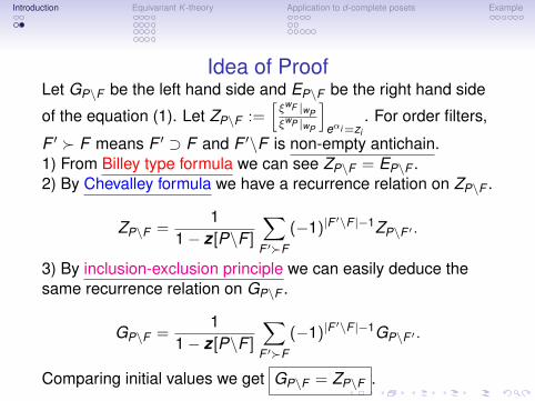
Idea of ProofLet GP\F be the left hand side and EP\F be the right hand side
of the equation (1). Let ZP\F :=[ξwF |wPξwP |wP
]eαi =zi
. For order filters,
F ′ � F means F ′ ⊃ F and F ′\F is non-empty antichain.1) From Billey type formula we can see ZP\F = EP\F .2) By Chevalley formula we have a recurrence relation on ZP\F .
ZP\F =1
1− z[P\F ]
∑F ′�F
(−1)|F′\F |−1ZP\F ′ .
3) By inclusion-exclusion principle we can easily deduce thesame recurrence relation on GP\F .
GP\F =1
1− z[P\F ]
∑F ′�F
(−1)|F′\F |−1GP\F ′ .
Comparing initial values we get GP\F = ZP\F .

Introduction Equivariant K -theory Application to d-complete posets Example
Idea of ProofLet GP\F be the left hand side and EP\F be the right hand side
of the equation (1). Let ZP\F :=[ξwF |wPξwP |wP
]eαi =zi
. For order filters,
F ′ � F means F ′ ⊃ F and F ′\F is non-empty antichain.1) From Billey type formula we can see ZP\F = EP\F .2) By Chevalley formula we have a recurrence relation on ZP\F .
ZP\F =1
1− z[P\F ]
∑F ′�F
(−1)|F′\F |−1ZP\F ′ .
3) By inclusion-exclusion principle we can easily deduce thesame recurrence relation on GP\F .
GP\F =1
1− z[P\F ]
∑F ′�F
(−1)|F′\F |−1GP\F ′ .
Comparing initial values we get GP\F = ZP\F .

Introduction Equivariant K -theory Application to d-complete posets Example
OutlineIntroduction
Main TheoremIdea of Proof
Equivariant K -theoryKashiwara thick flag variety G/P−Equivariant K -theory KT (G/P−) and localization mapLittlewood-Richardson coefficientsChevalley formula
Application to d-complete posetsSetupBilley type formulaChevalley formula for d-complete poset
ExampleBirds

Introduction Equivariant K -theory Application to d-complete posets Example
Kashiwara thick flag variety G/P−A = (aij)i,j∈I a symmetrizable generalized Cartan matrix,
Γ the corresponding Dynkin diagram with node set I.
Then the associated Kac–Moody group G over C is constructedfrom the following data:
the weight lattice Z-module Λ ' Zm,the (linearly independent) simple roots Π = {αi : i ∈ I} ⊂ Λ,
the simple coroots Π∨ = {α∨i : i 3 I} ⊂ Λ∗,the fundamental weights {λi : i ∈ I} ⊂ Λ
where Λ∗ = HomZ(Λ,Z) is the dual lattice. We will write thecanonical pairing 〈 , 〉 : Λ∗ × Λ→ Z. These satisfy
〈α∨i , αj〉 = aij , 〈α∨i , λj〉 = δij .

Introduction Equivariant K -theory Application to d-complete posets Example
The Weyl group W is generated by simple reflections si (i ∈ I)and it is known to be a crystallographic Coxeter group.
Let B be a Borel subgroup and B− the opposite Borel i.e.B ∩ B− = T is the maximal torus.
Let us fix a subset J ( I. Then we can consider the subgroupWJ ⊂W generated by sj , (j ∈ J) and the parabolic subgroupP− ⊃ B− corresponding to J.
Let W J = W/WJ be the set of minimum length cosetrepresentatives.Then we can consider
the Kashiwara thick partial flag variety XP− = G/P−.

Introduction Equivariant K -theory Application to d-complete posets Example
XP− = G/P− has cell decomposition.
XP− =⊔
w∈W J
X ◦w
where X ◦w = BwP−/P− is the B-orbit of T -fixed pointcorresponding to w , ew = wP−/P− ∈ XP− .The Zariski closure Xw = X ◦w of X ◦w is called the Schubertvariety.Using Bruhat order ≤ on W J induced from W , we have celldecomposition
Xw =⊔
u∈W J ,u≥w
X ◦u .
Xw has codimension `(w) in XP− and it is infinite dimensional if|W | =∞.

Introduction Equivariant K -theory Application to d-complete posets Example
OutlineIntroduction
Main TheoremIdea of Proof
Equivariant K -theoryKashiwara thick flag variety G/P−Equivariant K -theory KT (G/P−) and localization mapLittlewood-Richardson coefficientsChevalley formula
Application to d-complete posetsSetupBilley type formulaChevalley formula for d-complete poset
ExampleBirds

Introduction Equivariant K -theory Application to d-complete posets Example
Equivariant K -theory KT (G/P−)We can consider T -equivariant K -theory of XP− = G/P−KT (G/P−) is the Grothendieck group of coherent sheaves onG/P−. It has ring structure and
KT (XP−) ∼=∏
w∈W J
KT (pt)[Ow ],
where Ow is the structure sheaf of the Schubert variety Xw and[Ow ] is the corresponding class in KT (XP−).KT (pt) is the T -equivariant K -theory of a point and it can beidentified with the representation ring of T .
KT (pt) ' R(T ) ' Z[Λ].
Each element in Z[Λ] is expressed as a (Z-)linear combinationof eλ (λ ∈ Λ). eλ corresponds to the class of line bundle Lλ withcharacter λ.

Introduction Equivariant K -theory Application to d-complete posets Example
Schubert class and Localization map
For w ∈W J , we will write ξw = [Ow ] ∈ KT (XP−) and call itT -equivariant Schubert class.Each v ∈W J gives a T -fixed point ev = vP−/P− ∈ X . Thenthe inclusion map ιv : {ev} → X induces the pull-back ringhomomorphism, called the localization map at v ,
ι∗v : KT (XP−)→ KT (ev ) ∼= Z[Λ].
For two elements v , w ∈W J , we denote by ξw |v the image ofξw under the localization map ι∗v :
ξw |v = ι∗v ([Ow ]).

Introduction Equivariant K -theory Application to d-complete posets Example
Billey type formula for ξw |v
(Lam-Schilling-Shimozono 2010)
PropositionLet v, w ∈W J , and fix a reduced expression v = si1si2 . . . siN ofv. Then we have
ξw |v =∑
(k1,...,kr )
(−1)r−l(w)r∏
a=1
(1− eβ
(ka)), (2)
where the summation is taken over all sequences (k1, . . . , kr )such that 1 ≤ k1 < k2 < · · · < kr ≤ N and sik1
∗ · · · ∗ sikr= w
(with respect to the Demazure product), and β(k) is given byβ(k) = si1 . . . sik−1(αik ) for 1 ≤ k ≤ N.
Introduction Equivariant K -theory Application to d-complete posets Example
OutlineIntroduction
Main TheoremIdea of Proof
Equivariant K -theoryKashiwara thick flag variety G/P−Equivariant K -theory KT (G/P−) and localization mapLittlewood-Richardson coefficientsChevalley formula
Application to d-complete posetsSetupBilley type formulaChevalley formula for d-complete poset
ExampleBirds

Introduction Equivariant K -theory Application to d-complete posets Example
Littlewood-Richardson coefficientsWe consider the structure constants for the multiplication inKT (X ) with respect to the Schubert classes.
[Ou][Ov ] =∑
w∈W J
cwu,v [Ow ],
where u, v , w ∈W J , cwu,v ∈ KT (pt).
LemmaIf cw
u,v 6= 0, then u ≤ w and v ≤ w.
LemmaFor u, w ∈W J , we have
cwu,w = ξu|w . (3)
Introduction Equivariant K -theory Application to d-complete posets Example
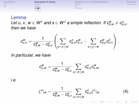
LemmaLet u, v, w ∈W J and s ∈W J a simple reflection. If cw
s,w 6= cus,u,
then we have
cwu,v =
1cw
s,w − cus,u
∑u<x≤w
cxs,ucw
x ,v −∑
u≤y<w
cws,ycy
u,v
.
In particular, we have
cwu,w =
1cw
s,w − cus,u
∑u<x≤w
cxs,ucw
x ,w .
i.e.
ξu|w =1
cws,w − cu
s,u
∑u<x≤w
cxs,uξ
x |w . (4)

Introduction Equivariant K -theory Application to d-complete posets Example
Proof.Consider the associativity
([Os][Ou]) [Ov ] = [Os] ([Ou][Ov ])
and take the coefficients of [Ow ] in the both hand sides.
cus,ucw
u,v +∑
u<x≤w
cxs,ucw
x ,v = cws,wcw
u,v +∑
u≤y<w
cws,ycy
u,v ,
then we get
cwu,v =
1cw
s,w − cus,u
∑u<x≤w
cxs,ucw
x ,v −∑
u≤y<w
cws,ycy
u,v
.

Introduction Equivariant K -theory Application to d-complete posets Example
OutlineIntroduction
Main TheoremIdea of Proof
Equivariant K -theoryKashiwara thick flag variety G/P−Equivariant K -theory KT (G/P−) and localization mapLittlewood-Richardson coefficientsChevalley formula
Application to d-complete posetsSetupBilley type formulaChevalley formula for d-complete poset
ExampleBirds

Introduction Equivariant K -theory Application to d-complete posets Example
T -quivariant Chevalley formulaW -orbit of the set of simple roots Π(resp. simple coroots Π∨)determine the set of real roots (resp. real coroots)
Φ = W Π (resp. Φ∨ = W Π∨)
and the decomposition of Φ (resp. Φ∨) into the positive systemΦ+ (resp. Φ∨+) and the negative system Φ− (resp. Φ∨−).For a dominant weight λ ∈ Λ, we define
Hλ = {(γ∨, k) : γ∨ ∈ Φ∨+,0 ≤ k < 〈γ∨, λ〉, k ∈ N}.
Fix a total order on the Dynkin node I so that I = {i1 < · · · < ir}.define a map ι : Hλ → Qr+1 by
ι
r∑j=1
ciα∨ij , k
=1
〈γ∨, λ〉(k , c1, · · · , cr ) .
Then it is known that ι is injective.

Introduction Equivariant K -theory Application to d-complete posets Example
We define a total ordering < on Hλ by
h < h′ ⇐⇒ ι(h) <lex ι(h′),
where <lex is the lexicographical ordering on Qr+1. Forh = (γ∨, k), we define affine transformations rh and r̃h on Λ by
rh(µ) = µ− 〈γ∨, µ〉γ,r̃h(µ) = rh(µ) +
(〈γ∨, λ〉 − k
)γ.
Note that rh = sγ is the reflection corresponding to the positiveroot γ.

Introduction Equivariant K -theory Application to d-complete posets Example
Lenart-Shimozono (2014)
PropositionLet s = si ∈W J be a simple reflection. Then for w , v ∈W J wehave
cws,v =
1− eλi−vλi if w = v ,∑(h1,··· ,hr )
(−1)r−1eλi−v r̃h1···̃rhr λi if w > v, (5)
where the summation is taken over all sequences (h1, · · · ,hr )of length r ≥ 1 satisfying the following two conditions:
(H1) h1 > h2 > · · · > hr in Hλi ,(H2) v l vrh1 l vrh1rh2 l · · ·l vrh1 · · · rhr = w is a saturated chain
in W J .

Introduction Equivariant K -theory Application to d-complete posets Example
OutlineIntroduction
Main TheoremIdea of Proof
Equivariant K -theoryKashiwara thick flag variety G/P−Equivariant K -theory KT (G/P−) and localization mapLittlewood-Richardson coefficientsChevalley formula
Application to d-complete posetsSetupBilley type formulaChevalley formula for d-complete poset
ExampleBirds
Introduction Equivariant K -theory Application to d-complete posets Example
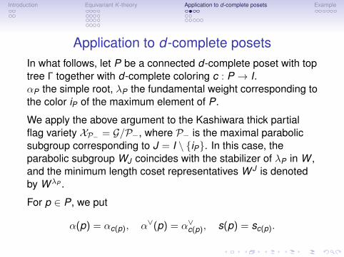
Application to d-complete posetsIn what follows, let P be a connected d-complete poset with toptree Γ together with d-complete coloring c : P → I.αP the simple root, λP the fundamental weight corresponding tothe color iP of the maximum element of P.
We apply the above argument to the Kashiwara thick partialflag variety XP− = G/P−, where P− is the maximal parabolicsubgroup corresponding to J = I \ {iP}. In this case, theparabolic subgroup WJ coincides with the stabilizer of λP in W ,and the minimum length coset representatives W J is denotedby W λP .
For p ∈ P, we put
α(p) = αc(p), α∨(p) = α∨c(p), s(p) = sc(p).
Introduction Equivariant K -theory Application to d-complete posets Example
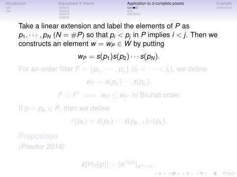
Take a linear extension and label the elements of P asp1, · · · ,pN (N = #P) so that pi < pj in P implies i < j . Then weconstructs an element w = wP ∈W by putting
wP = s(p1)s(p2) · · · s(pN).
For an order filter F = {pi1 , · · · ,pir } (i1 < · · · < ir ), we define
wF = s(pi1) · · · s(pir ).
F ⊂ F ′ ⇐⇒ wF ≤ wF ′ in Bruhat order
If p = pk ∈ P, then we define
β(pk ) = s(p1) · · · s(pk−1)α(pk ),
Proposition(Proctor 2014)
z[HP(p)] = [eβ(p)]eαi =zi .
Introduction Equivariant K -theory Application to d-complete posets Example
Take a linear extension and label the elements of P asp1, · · · ,pN (N = #P) so that pi < pj in P implies i < j . Then weconstructs an element w = wP ∈W by putting
wP = s(p1)s(p2) · · · s(pN).
For an order filter F = {pi1 , · · · ,pir } (i1 < · · · < ir ), we define
wF = s(pi1) · · · s(pir ).
F ⊂ F ′ ⇐⇒ wF ≤ wF ′ in Bruhat order
If p = pk ∈ P, then we define
β(pk ) = s(p1) · · · s(pk−1)α(pk ),
Proposition(Proctor 2014)
z[HP(p)] = [eβ(p)]eαi =zi .

Introduction Equivariant K -theory Application to d-complete posets Example
Given a subset D = {pi1 , · · · ,pir } (i1 < · · · < ir ) of P, we defineelements wD ∈W and w∗D ∈W by putting
wD = s(pi1)s(pi2) · · · s(pir ) and w∗D = s(pi1) ∗ s(pi2) ∗ · · · ∗ s(pir ),
where ∗ is the Demazure product.
PropositionLet F be an order filter of P and D ⊂ P.(1) D ∈ EP(F ) ⇐⇒ wD = wF and |E | = |F |(2) D ∈ E∗P(F ) ⇐⇒ w∗D = wFFor the case (2) D is uniquely expressed asD = D′ t S s.t. D′ ∈ EP(F ),S ⊂ B(D′).

Introduction Equivariant K -theory Application to d-complete posets Example
OutlineIntroduction
Main TheoremIdea of Proof
Equivariant K -theoryKashiwara thick flag variety G/P−Equivariant K -theory KT (G/P−) and localization mapLittlewood-Richardson coefficientsChevalley formula
Application to d-complete posetsSetupBilley type formulaChevalley formula for d-complete poset
ExampleBirds

Introduction Equivariant K -theory Application to d-complete posets Example
Billey type formulaPropositionWe have
ξwF |wP =∑
E∈E∗P (F )
(−1)#E−#F∏p∈E
(1− z[HP(p)]) , (6)
under the identification zi = eαi (i ∈ I). We can rewrite theabove expression as
ξwF |wP =∑
D∈EP(F )
∏p∈D
(1− z[HP(p)])∏
p∈B(D)
z[HP(p)].
ξwF |wP
ξwP |wP
=∑
D∈EP(F )
∏v∈B(D) z[HP(v)]∏
v∈P\D(1− z[HP(v)])

Introduction Equivariant K -theory Application to d-complete posets Example
OutlineIntroduction
Main TheoremIdea of Proof
Equivariant K -theoryKashiwara thick flag variety G/P−Equivariant K -theory KT (G/P−) and localization mapLittlewood-Richardson coefficientsChevalley formula
Application to d-complete posetsSetupBilley type formulaChevalley formula for d-complete poset
ExampleBirds
Introduction Equivariant K -theory Application to d-complete posets Example
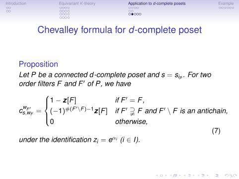
Chevalley formula for d-complete poset
PropositionLet P be a connected d-complete poset and s = siP . For twoorder filters F and F ′ of P, we have
cwF ′s,wF
=
1− z[F ] if F ′ = F,(−1)#(F ′\F )−1z[F ] if F ′ % F and F ′ \ F is an antichain,0 otherwise,
(7)under the identification zi = eαi (i ∈ I).
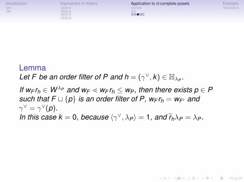
Introduction Equivariant K -theory Application to d-complete posets Example
LemmaLet F be an order filter of P and h = (γ∨, k) ∈ HλP .
If wF rh ∈W λP and wF l wF rh ≤ wP , then there exists p ∈ Psuch that F t {p} is an order filter of P, wF rh = wF ′ andγ∨ = γ∨(p).In this case k = 0, because 〈γ∨, λP〉 = 1, and r̃hλP = λP .

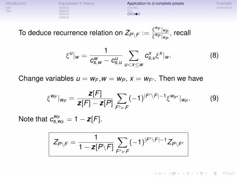
Introduction Equivariant K -theory Application to d-complete posets Example
To deduce recurrence relation on ZP\F :=ξwF |wPξwP |wP
, recall
ξu|w =1
cws,w − cu
s,u
∑u<x≤w
cxs,uξ
x |w . (8)
Change variables u = wF ,w = wP , x = wF ′ . Then we have
ξwF |wP =z[F ]
z[F ]− z[P]
∑F ′�F
(−1)|F′\F |−1ξwF ′ |wP . (9)
Note that cwFs,wF
= 1− z[F ].
ZP\F =1
1− z[P\F ]
∑F ′�F
(−1)|F′\F |−1ZP\F ′

Introduction Equivariant K -theory Application to d-complete posets Example
Remark
Stembridge (2001) classified dominant λ-minuscule element ofWeyl groups and found another two families other than15-classes of Proctor’s. , which are the cases of non-simplylaced Dynkin diagrams. All our arguments can be applied tothese cases.Replace colored d-complete posets by a heap H(w) of adominant λ-minuscule element w .Definitions of EP(F ) and B(D) should be slightly modified.Then the same ED-hook type formula of the theorem holds.

Introduction Equivariant K -theory Application to d-complete posets Example
OutlineIntroduction
Main TheoremIdea of Proof
Equivariant K -theoryKashiwara thick flag variety G/P−Equivariant K -theory KT (G/P−) and localization mapLittlewood-Richardson coefficientsChevalley formula
Application to d-complete posetsSetupBilley type formulaChevalley formula for d-complete poset
ExampleBirds

Introduction Equivariant K -theory Application to d-complete posets Example
Smallest Bird
1
2 3 4
5
6
7 8
9 10
Figure: e6[1; 2,2]

Introduction Equivariant K -theory Application to d-complete posets Example
Example1
2 3 4
5
6
7 8
9 10
1
2 3 4
5
6
2 3
5 1
z[1] = z1z22 z2
3 z4z25 z6,
z[2] = z1z2z3z4z5z6,z[3] = z1z2z3z4z5,z[4] = z3z4,z[5] = z1z2z3z5z6,z[6] = z5z6,z[7] = z1z2z3z5,z[8] = z3,z[9] = z5,
z[10] = z1.
∆[P] =10∏
i=1
(1− z[i])
There are 29 order filters.F7 = {1, 2, 3, 5}EP (F7) = {{1, 2, 3, 5}, {1, 2, 5, 8}, {1, 2, 3, 9}, {1, 2, 8, 9}, {1, 7, 8, 9}},
GP/F7=
(1−z[1])(1−z[2])(1−z[3])(1−z[5])∆(P)
+(1−z[1])(1−z[2])(1−z[5])(1−z[8])z[3]
∆(P)+
(1−z[1])(1−z[2])(1−z[3])(1−z[9])z[5]∆(P)
+(1−z[1])(1−z[2])(1−z[8])(1−z[9])z[3]z[5]
∆(P)+
(1−z[1])(1−z[7])(1−z[8])(1−z[9])z[2]∆(P)
=(1−z[1])F (z)
∆(P)
where F (z) = 1− z1z2z23 z4z5 − z1z2z2
3 z4z5z6 − z1z2z3z25 z6 − z1z2z3z4z2
5 z6 + z1z2z23 z4z2
5 z6 −z2
1 z22 z2
3 z4z25 z6 + z2
1 z22 z3
3 z4z25 z6 + z2
1 z22 z3
3 z24 z2
5 z6 + z21 z2
2 z23 z4z3
5 z6 + z21 z2
2 z23 z4z3
5 z26 − z3
1 z32 z4
3 z24 z4
5 z26 .

Introduction Equivariant K -theory Application to d-complete posets Example
B3 example
B3 Dynkin diagram s0 = s1 − s2w = s0(s1s0)(s2s1s0) λ0-minuscules0 s1 s2
s0 s1
s0
β1 β2 β3
β4 β5
β6
γ∨1 γ∨2 γ∨3γ∨4 γ∨5
γ∨6
β1 = α0 + α1 + α2 , β2 = 2α0 + 2α1 + α2 , β3 = 2α0 + α1 + α2β4 = α0 + α1, β5 = 2α0 + α1, β6 = α0,
γ∨1 = α∨0 , γ∨2 = α∨0 + α∨1 , γ∨3 = α∨0 + α∨1 + α∨2 ,γ∨4 = α∨0 + 2α∨1 , γ∨5 = α∨0 + 2α∨1 + α∨2 , γ∨6 = α∨0 + 2α∨1 + 2α∨2
Introduction Equivariant K -theory Application to d-complete posets Example
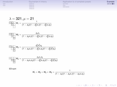
λ = 321, µ = 21��
�W1 =
1
(1− z0)(1− z20 z1)(1− z2
0 z1z2)
��◦�
W2 =z0z1
(1− z0z1)(1− z20 z1)(1− z2
0 z1z2)
� ◦��
W3 =z2
0 z21 z2
(1− z0z1)(1− z20 z1z2)(1− z2
0 z21 z2)
◦��
�
W4 =z0z1z2
(1− z0z1z2)(1− z20 z1z2)(1− z2
0 z21 z2)
ED-sum
W1 + W2 + W3 + W4 =1
(1− z0)(1− z0z1)(1− z0z1z2)

Introduction Equivariant K -theory Application to d-complete posets Example
Thank you!