Equity free cash flow based approach to valuation of credit default option embedded

in project finance

Abstract

In this paper we present a novel approach towards the financial rationality assessment of

commercial real estate developments being realized within a project finance framework. The

proposed solution is based on Cox Ross Rubinstein (CRR) binomial lattice that is utilized to

assess the price of the loan default option inherent to the financing structure of these types of

projects and, consequently, their values for equity providers.

The research gap addressed in this work originates from two main sources. Firstly, our solution

of default option valuation is based on equity cash flow (ECF) - an approach commonly used

in project finance and analysis of real estate projects, which according to our knowledge, has

not been yet applied for such purpose. We argue that real estate projects, executed in a given

project finance framework, due to their high leverage and nonrecourse debt obligations,

contain embedded and particularly valuable default options and thus for practical reasons

investors require real options financial layout that is based on discounted ECF. Secondly, the

commonly used valuation techniques of real options included in real estate projects do not take

full advantage of CRR ability to valuate real options for changing the value of the exercise

price, which in the case of real estate projects, arises from the structured development of loan

taking and repayment. Furthermore, contrary to closed form option pricing formulas, the

presented method makes it possible to identify the optimal moment of option execution based

on the loan to value ratio. In cases where the value of equity is lower than 0, rationally acting

investors should abandon the project.

We support our solution with a case study embedded within a professional framework,

providing further contribution to the research and practitioners’ community.

1. Introduction

In today’s turbulent economic reality and in the context of dynamically changing real estate

market conditions, effective and strategically viable investment decisions become even more

difficult. This situation presents multiple challenges for financial analytics, and directly exposes

various deficiencies of typical DCF based investment valuation techniques, whose drawbacks

have been thoroughly studied in the past by many authors (Feinstein and Lander (2002);….)

The introduction of the real options concept by Stewart Myers in 1977 (Myers 1977) created a

new theoretical and practical environment that allowed to address some of these issues by

recognizing the strategic nature of investment process and provided rational explanation of the

investors behavior and approach towards project risk assessment. This crucial concept behind

the so-called “real option valuation” is based on the observation that investors are able to

reduce the probability of project negative outcome through active management and

consecutive decisions made upon the arrival of revised project or market data. In particular,

the real options approach has been employed to explain how the existence of nonrecourse

debt obligations in projects affects their intrinsic value and presents the advantages that such

knowledge may bring to investors analyzing the financial rationality of a given endeavor

(Gendrin, Lai, Soumare, 2007).

From this point of view, having several available discounting methods to choose from

(Fernandez, 2007), much of the research efforts has been focused on FCF as a platform for

real options analytics (Luehrman 1998; Amram and Kalitulake, 1999; Trigeorgis, 1999).

Unfortunately, application of such models, in the case of many real estate projects

implemented within a given project finance framework has a limited practical usage. In the

case of such projects, direct focus on investors’ returns, straightforward benchmarking with

other alternative investments and the fact that the vast majority of ventures are project-financed

has led to a situation where the methodology which dominated the real estate practice is the

one based on equity cash flows. Its advantages for large-scale project valuation, which

requires significant capital investment volumes, has been recognized and attempts have been

made to improve its accuracy and applicability within the project framework (Esty, 1999).

The conducted literature review has revealed only one existing model (Winsen, 2010) which

employs binomial option structure to value non-recourse loan in project finance. In contrary to

that, our paper focuses on providing a valuation framework for default option using equity cash

flow analysis, which by taking into account the investors’ position, should make it possible to

make more optimal business decisions. The proposed solution is also based on binomial trees,

which in comparison to closed form solutions, is distinguished by computational flexibility and

the possibility of determining the optimal moment of option exercise through investment

abandon decision over the entire project lifespan. In addition, our model assumes that at each

stage of the project, the logic behind the investor behavior induces two different sets of actions

depending on loan to value ratio of the property (which in the case of real estate projects

typically corresponds to the majority of investment vehicle value):

- If equity value is higher than zero, i.e. the project value exceeds the remaining debt balance,

the investors will choose to continue their engagement in the project and keep settling their

credit liabilities (repayment), alternatively

- If equity value is lower than zero, i.e. the project value is lower than the remaining loan

balance, the investors will decide to exit the project by ceasing to repay the loan.

Given the fact that investors have the right but not the obligation to undertake such actions

without additional financial recourses, their perception of the project risk should decrease,

having also a positive impact on their project financial rationality assessment.

The remaining part of the article is organized as follows. In Section 2, we present the theoretical

background of the equity free cash flow based approach to valuation of credit default option

embedded in project finance. Section 3 contains our case study which presents application of

the introduced methodology in a professional environment. Section 4 presents our concluding

remarks.

2. The model

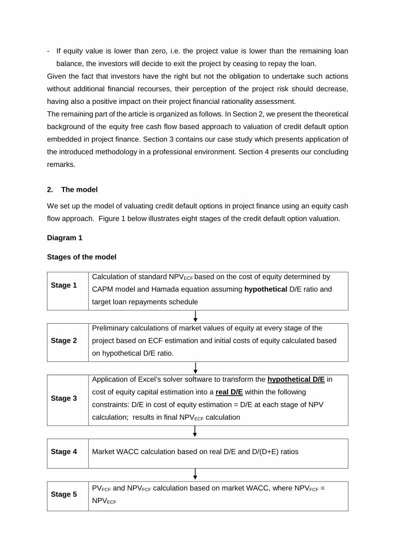
We set up the model of valuating credit default options in project finance using an equity cash

flow approach. Figure 1 below illustrates eight stages of the credit default option valuation.

Diagram 1

Stages of the model

Stage 1 Calculation of standard NPVECF based on the cost of equity determined by

CAPM model and Hamada equation assuming hypothetical D/E ratio and

target loan repayments schedule

Stage 2

Preliminary calculations of market values of equity at every stage of the

project based on ECF estimation and initial costs of equity calculated based

on hypothetical D/E ratio.

Stage 3

Application of Excel’s solver software to transform the hypothetical D/E in

cost of equity capital estimation into a real D/E within the following

constraints: D/E in cost of equity estimation = D/E at each stage of NPV

calculation; results in final NPVECF calculation

Stage 4 Market WACC calculation based on real D/E and D/(D+E) ratios

Stage 5 PVFCF and NPVFCF calculation based on market WACC, where NPVFCF =

NPVECF

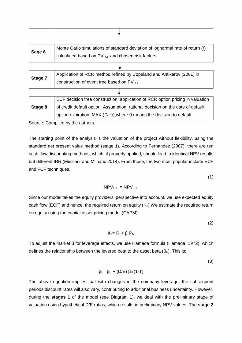
Sage 6 Monte Carlo simulations of standard deviation of lognormal rate of return (r)

calculated based on PVFCF and chosen risk factors

Stage 7 Application of RCR method refined by Copeland and Antikarov (2001) in

construction of event tree based on PVFCF

Stage 8

ECF decision tree construction; application of RCR option pricing in valuation

of credit default option. Assumption: rational decision on the date of default

option expiration: MAX (��; 0),where 0 means the decision to default

Source: Compiled by the authors.

The starting point of the analysis is the valuation of the project without flexibility, using the

standard net present value method (stage 1). According to Fernandez (2007), there are ten

cash flow discounting methods, which, if properly applied, should lead to identical NPV results

but different IRR (Mielcarz and Mlinarič 2014). From those, the two most popular include ECF

and FCF techniques.

(1)

NPVFCF = NPVECF

Since our model takes the equity providers’ perspective into account, we use expected equity

cash flow (ECF) and hence, the required return on equity (Ke).We estimate the required return

on equity using the capital asset pricing model (CAPM):

(2)

Ke= RF+ βLPM

To adjust the market β for leverage effects, we use Hamada formula (Hamada, 1972), which

defines the relationship between the levered beta to the asset beta (βU). This is:

(3)

βL= βU + (D/E) βU (1-T)

The above equation implies that with changes in the company leverage, the subsequent

periods discount rates will also vary, contributing to additional business uncertainty. However,

during the stages 1 of the model (see Diagram 1), we deal with the preliminary stage of

valuation using hypothetical D/E ratios, which results in preliminary NPV values. The stage 2

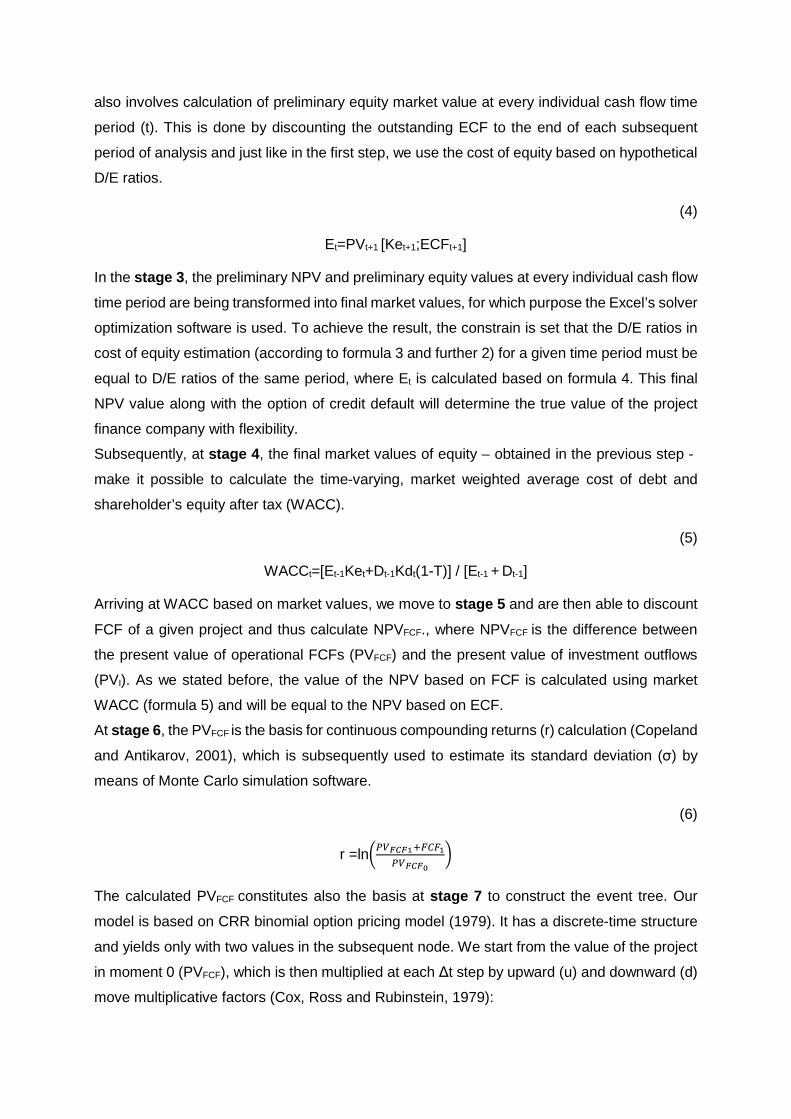
also involves calculation of preliminary equity market value at every individual cash flow time

period (t). This is done by discounting the outstanding ECF to the end of each subsequent

period of analysis and just like in the first step, we use the cost of equity based on hypothetical

D/E ratios.

(4)

Et=PVt+1 [Ket+1;ECFt+1]

In the stage 3, the preliminary NPV and preliminary equity values at every individual cash flow

time period are being transformed into final market values, for which purpose the Excel’s solver

optimization software is used. To achieve the result, the constrain is set that the D/E ratios in

cost of equity estimation (according to formula 3 and further 2) for a given time period must be

equal to D/E ratios of the same period, where Et is calculated based on formula 4. This final

NPV value along with the option of credit default will determine the true value of the project

finance company with flexibility.

Subsequently, at stage 4, the final market values of equity – obtained in the previous step -

make it possible to calculate the time-varying, market weighted average cost of debt and

shareholder’s equity after tax (WACC).

(5)

WACCt=[Et-1Ket+Dt-1Kdt(1-T)] / [Et-1 + Dt-1]

Arriving at WACC based on market values, we move to stage 5 and are then able to discount

FCF of a given project and thus calculate NPVFCF., where NPVFCF is the difference between

the present value of operational FCFs (PVFCF) and the present value of investment outflows

(PVI). As we stated before, the value of the NPV based on FCF is calculated using market

WACC (formula 5) and will be equal to the NPV based on ECF.

At stage 6, the PVFCF is the basis for continuous compounding returns (r) calculation (Copeland

and Antikarov, 2001), which is subsequently used to estimate its standard deviation (σ) by

means of Monte Carlo simulation software.

(6)

r =ln����� � ����

�

The calculated PVFCF constitutes also the basis at stage 7 to construct the event tree. Our

model is based on CRR binomial option pricing model (1979). It has a discrete-time structure

and yields only with two values in the subsequent node. We start from the value of the project

in moment 0 (PVFCF), which is then multiplied at each Δt step by upward (u) and downward (d)

move multiplicative factors (Cox, Ross and Rubinstein, 1979):

(7)

� = ��√∆�

And

(8)

� = ���√∆�

In accordance with Copeland and Antikarov (2001), after determining the value of the project

at the first stage, we should consider the payout ratio (pr) of FCF during each stage of project

execution:

(9)

prt= � �

���[�����; � �]

Having the present value of the project before FCF distribution PVFCF(i,t), where i is the number

of downward project value moves and t is the time period of free cash flow payment, we

calculate it by applying u and d factors, so that:

(10)

PVFCF (i,t+1)= PVFCF (i,t)u

and

(11)

PVFCF (i+1,t+1)= PVFCF (i,t)d

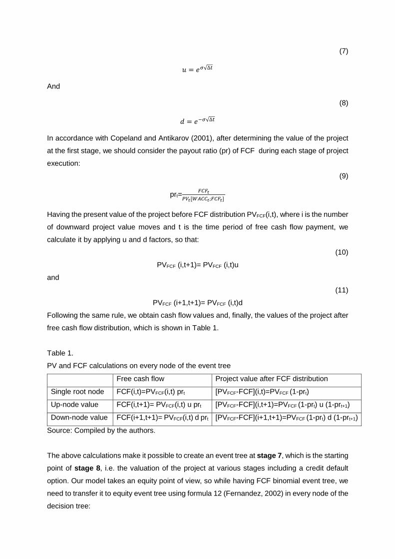
Following the same rule, we obtain cash flow values and, finally, the values of the project after

free cash flow distribution, which is shown in Table 1.

Table 1.

PV and FCF calculations on every node of the event tree

Free cash flow Project value after FCF distribution

Single root node FCF(i,t)=PVFCF(i,t) prt [PVFCF-FCF](i,t)=PVFCF (1-prt)

Up-node value FCF(i,t+1)= PVFCF(i,t) u prt [PVFCF-FCF](i,t+1)=PVFCF (1-prt) u (1-prt+1)

Down-node value FCF(i+1,t+1)= PVFCF(i,t) d prt [PVFCF-FCF](i+1,t+1)=PVFCF (1-prt) d (1-prt+1)

Source: Compiled by the authors.

The above calculations make it possible to create an event tree at stage 7, which is the starting

point of stage 8, i.e. the valuation of the project at various stages including a credit default

option. Our model takes an equity point of view, so while having FCF binomial event tree, we

need to transfer it to equity event tree using formula 12 (Fernandez, 2002) in every node of the

decision tree:

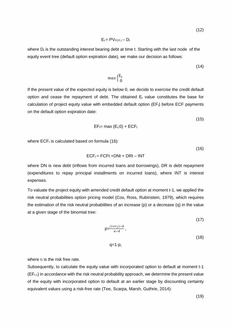
(12)

Et = PVFCF,t – Dt

where Dt is the outstanding interest bearing debt at time t. Starting with the last node of the

equity event tree (default option expiration date), we make our decision as follows:

(14)

� ! "E� 0

If the present value of the expected equity is below 0, we decide to exercise the credit default

option and cease the repayment of debt. The obtained Et value constitutes the base for

calculation of project equity value with embedded default option (EFt) before ECF payments

on the default option expiration date:

(15)

EFt= max (Et;0) + ECFt

where ECFt is calculated based on formula (16):

(16)

ECFt = FCFt +DNt + DRt – INT

where DN is new debt (inflows from incurred loans and borrowings), DR is debt repayment

(expenditures to repay principal installments on incurred loans), where INT is interest

expenses.

To valuate the project equity with amended credit default option at moment t-1, we applied the

risk neutral probabilities option pricing model (Cox, Ross, Rubinstein, 1979), which requires

the estimation of the risk neutral probabilities of an increase (p) or a decrease (q) in the value

at a given stage of the binomial tree:

(17)

p=(%�&')�(

)�( ,

(18)

q=1-p,

where rf is the risk free rate.

Subsequently, to calculate the equity value with incorporated option to default at moment t-1

(EFt-1) in accordance with the risk neutral probability approach, we determine the present value

of the equity with incorporated option to default at an earlier stage by discounting certainty

equivalent values using a risk-free rate (Tee, Scarpa, Marsh, Guthrie, 2014):

(19)

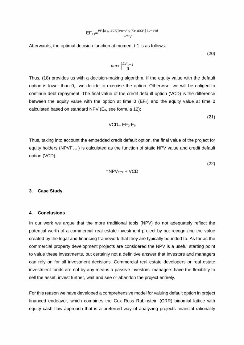
EFt-1=���[*+�;,� �]-)����[*+�;,� �] (%�-)(

%�&'

Afterwards, the optimal decision function at moment t-1 is as follows:

(20)

� ! "�.��%0

Thus, (18) provides us with a decision-making algorithm. If the equity value with the default

option is lower than 0, we decide to exercise the option. Otherwise, we will be obliged to

continue debt repayment. The final value of the credit default option (VCD) is the difference

between the equity value with the option at time 0 (EF0) and the equity value at time 0

calculated based on standard NPV (E0, see formula 12):

(21)

VCD= EF0-E0

Thus, taking into account the embedded credit default option, the final value of the project for

equity holders (NPVFECF) is calculated as the function of static NPV value and credit default

option (VCD):

(22)

=NPVECF + VCD

3. Case Study

4. Conclusions

In our work we argue that the more traditional tools (NPV) do not adequately reflect the

potential worth of a commercial real estate investment project by not recognizing the value

created by the legal and financing framework that they are typically bounded to. As for as the

commercial property development projects are considered the NPV is a useful starting point

to value these investments, but certainly not a definitive answer that investors and managers

can rely on for all investment decisions. Commercial real estate developers or real estate

investment funds are not by any means a passive investors: managers have the flexibility to

sell the asset, invest further, wait and see or abandon the project entirely.

For this reason we have developed a comprehensive model for valuing default option in project

financed endeavor, which combines the Cox Ross Rubinstein (CRR) binomial lattice with

equity cash flow approach that is a preferred way of analyzing projects financial rationality

assessment by vast majority of real estate investors. Our model is by no means limited to the

application presented in the case study. The study of various other commercial real estate

development or investment projects such as office or industrial can be performed in similar

fashion and other applications outside real estate industry could also probably be found.

In addition the presented approach encourages further works, in which the similar models can

be created by for example taking into account Lender’s perspective. In such case the equations

can be additionally fortified with analytics that recognizes that from the lender’s perspective its

position is spread between two options namely the upper one, which provides the shopping

center developer with the option to default against the lender, and the lower one which gives

the lender’s and option to default against the reinsurer. Such spread of two put option may

have further impact on both the investor’s and bank’s perception of the project viability.

Presumably the model would also help lender’s to determine an appropriate LTV level to

sufficiently cover the risk related to the default, which may vary depending on the price of the

option and as such can be implemented in the loan agreement.

Considering the above we treat our solution as a starting point for creating a set of models

which among other basic components of investors and manager’s toolkits such as other NPV,

payback rules or accounting rates of return should assist them in making even more effective

business decisions

References

Feinstein S., Lander D., A Better Understanding of Why NPV Undervalues Managerial

Flexibility, The Engineering Economist, 4, 2002.

Amram M., Kalitulake N., Real Options, Managing Strategic Investment in an Uncertain Word,

Harvard Business School Press, Boston 1999

Luehrman, T.A., Investment Opportunities as Real Options: Getting Started on the Numbers,

Harvard Business Review, 1998, 76, 4.

Peter Chinloy & James Musumeci, 1994, "Shopping Center Financing: Pricing Loan Default

Risk," Journal of Real Estate Research, American Real Estate Society, vol. 9(1), pages 49-64.

Lenos Trigeorgis, "Real options: Managerial flexibility and strategy in resource allocation”, The

MIT Press, Cambridge, MA, 1996, xiii + 427 pp. (hardcover), ISBN 0-262-20102-X

Pablo Fernández, (2007) "Valuing companies by cash flow discounting: ten methods and nine

theories", Managerial Finance, Vol. 33 Iss: 11, pp.853 – 876

Winsen, Joseph K. "An Overview of Project Finance Binomial Loan Valuation." Review of

Financial Economics : RFE 19.2 (2010).

Gendron, Michel. "Project Finance With Limited Recourse: An Option Pricing Approach to Debt

Capacity and Project Risk." The Journal of Structured Finance 13.3 (2007).

Myers, Stewart C., (1977), Determinants of corporate borrowing, 5, issue 2, p. 147-175,

Fernandez, Pablo and Linares, Pablo and Fernández Acín, Isabel, Market Risk Premium Used

in 88 Countries in 2014: A Survey with 8,228 Answers (June 20, 2014).

Esty, B. C. "Improved Techniques for Valuing Large-Scale Projects." Journal of Project

Finance 5, no. 1 (spring 1999): 9–25.