equilibrium concepts in differential information economies
TRANSCRIPT
Equilibrium conceptsin differential information economies
Dionysius Glycopantis1 and Nicholas C. Yannelis2
1 Department of Economics, City University, Northampton Square, London EC1V 0HB, UK(e-mail: [email protected])
2 Department of Economics,University of Illinois at Urbana-Champaign, IL 61820, USA(e-mail: [email protected])
Summary. We summarize here basic cooperative and noncooperative equilibriumconcepts, in the context of differential information economies with a finite numberof agents. These, on the one hand, game theoretic, and, on the other hand, Walrasianequilibrium type concepts are explained, and their relation is pointed out, in thecontext of specific economies with one or two goods and two or three agents.We analyze the incentive compatibility of several cooperative and noncooperativeconcepts, and also we discuss briefly the possible implementation of these conceptsas perfect Bayesian equilibria through the construction of relevant game trees. Thispossibility is related to whether the allocation is incentive compatible. This dependson whether there is free disposal or not.
Keywords and Phrases: Differential information economy, Walrasian expecta-tions or Radner equilibrium, Rational expectations equilibria, Free disposal, Weakfine core, Private core, Weak fine value, Private value, Coalitional Bayesian incen-tive compatibility, Game trees, Perfect Bayesian equilibrium, Sequential equilib-rium.
JEL Classification Numbers: D5, D82, C71, C72.
1 Introduction
The classical Walrasian equilibrium model as formalized by Arrow - Debreu (1954)and McKenzie (1954) consists of a finite set of agents each of which is characterized
We are very grateful to A. Muir for his invaluable help and suggestions. We wish to thank A.Hadjiprocopis for his invaluable help with the implementation of Latex in a Unix environment. Healso provided us with numerically approximate solutions to Radner equilibrium and weak fine valueproblems, using a random selection algorithm.

2 D. Glycopantis and N.C. Yannelis
by her preferences and initial endowments. The Walrasian model captures in adeterministic way the trade or contract (redistribution of initial endowments) amongthe agents and has played a central role in all aspects of economics. For this modelsignificant results have been obtained, i.e. existence and Pareto optimality of theWalrasian equilibrium, equivalence of the Walrasian equilibrium with the core, (seeDebreu and Scarf, 1963), and the relation between the core and the Shapley value,(see Emmons and Scafuri, 1985). These results have also been extended in infinitedimensional spaces (see for example Aumann, 1964; and the books of Hildenbrand,1974; Khan and Yannelis, 1991).
Although infinite dimensional commodity spaces do capture uncertainty, theydo not capture trade under asymmetric (or differential) information. On the otherhand, it should be noted that most trades in an economy are made by agents whoare asymmetrically informed and the need to introduce differential information intothe Cournot - Nash model and the Arrow- Debreu - McKenzie model was evidentin the seminal works of Harsanyi (1967) and Radner (1968). Their equilibriumconcepts are noncooperative and have found extensive applications. In seminalpapers, Wilson (1978) and Myerson (1982) introduced private information in thecooperative concepts of the core and the Shapley value respectively.
Briefly, the purpose of this paper is to survey the basic equilibrium conceptsin economies with differential information. We employ a set of examples of finiteeconomies which enable us to compare the outcomes that different equilibriumconcepts generate. Also, we examine the implementation and the incentive com-patibility of different equilibrium concepts.
Our survey differs from the two recent ones by Forges (1998), Forges et al.(2000) and Ichiishi and Yamazaki (2002). These papers follow the Harsanyi typemodel and focus on the devolopment of cooperative, core concepts. In contrast,we focus on the partition model, examine in detail additional concepts such asthe Shapley value and provide an extensive form foundation for the concepts weexamine. Furthermore we analyze the incentive compatibility of the different equi-librium concepts and consider their implementation as a perfect Bayesian equilib-rium (PBE). These considerations can help us to decide how to choose among theavailable equilibrium concepts the most appropriate one. We also provide severalilluminating examples which enable one to contrast and compare the different equi-librium notions. These examples could be especially useful to those who start workin the area.
A finite economy with differential information consists of a finite set of agentsand states of nature. Each agent is characterized by a random utility function, a ran-dom consumption set, random initial endowments, a private information set whichis a partition of the set of the states of nature, and a prior probability distributionon these states. For such an economy a number of cooperative and non-cooperativeequilibrium concepts have been developed.
We believe that the natural and intuitive way to proceed is to analyse conceptsin terms of measurability of allocations (Yannelis, 1991). In particular, as it is wellknown, (e.g. Prescott and Townsend, 1984; Allen, 2003), without measurability, theset of feasible and incentive compatible allocations is not convex and therefore theexistence of an incentive compatible core becomes a serious problem. On the other
Equilibrium concepts in differential information economies 3
hand certain measurability conditions imply incentive compatibility and they helpus to narrow down the set of admissible allocations to a more manageable equilib-rium set which is not only incentive compatibility but also exists. It is precisely forthis reason that we follow the measurability approach.
We concentrate here mainly on cooperative concepts which allow for differenttypes of measurability of the proposed allocations, i.e. for alternative forms ofinformation sharing among the agents. In particular we consider the private core,(Yannelis, 1991), which is the set of all state-wise feasible and private informationmeasurable allocations that cannot be dominated, in terms of expected utility, byany coalition’s feasible and private information measurable net trades, the weak finecore (WFC), defined inYannelis (1991) and Koutsougeras andYannelis (1993), andthe concepts of private value and the weak fine value (WFV), (Krasa and Yannelis,1994), which employ the Shapley value.1
On the other hand we discuss the noncooperative concepts of the generalizedWalrasian equilibrium type ideas of Radner equilibrium, defined in Radner (1968),and rational expectations equilibrium (REE), which is discussed in Radner (1979),Allen (1981), Einy et al. (2000), Kreps (1977) and Laffont (1985) and Grossman(1981), among others. Unlike the Walrasian equilibrium, Radner equilibrium withpositive prices or REE may not exist in well behaved economies.
The paper is organized as follows. Section 2 contains the definition of a differ-entiable information economy. Section 3 defines cooperative equilibrium concepts.Section 4 defines noncooperative equilibrium concepts and makes some compar-isons between the various ideas. Section 5 applies the equilibrium ideas in thecontext of one-good and Section 6 in that of two-good examples. Section 7 visitsthe incentive compatibility idea and Section 8 discusses implementation or non-implementation properties, in terms of PBE, of various equilibrium notions. Sec-tion 9 pays special attention to the relation between REE and weak core conceptsand Section 10 concludes the discussion with some remarks. Finally Appendix Idiscusses some relations between core concepts.
2 Differential information economy (DIE)
In this section we define the notion of a finite-agent economy with differentialinformation for the case where the set of states of nature, Ω and the number ofgoods, l, per state are finite. I is a set of n players and Rl
+ will denote the set ofpositive real numbers.
A differential information exchange economy E is a set
((Ω,F), Xi,Fi, ui, ei, qi) : i = 1, . . . , n
where
1. F is a σ-algebra generated by a partition of Ω;2. Xi : Ω → 2R
l+ is the set-valued function giving the random consumption set
of Agent (Player) i, who is denoted by Pi;
1 See also Allen and Yannelis (2001) for additional references.

4 D. Glycopantis and N.C. Yannelis
3. Fi is a partition of Ω generating a sub-σ-algebra of F , denoting the privateinformation2 of Pi; Fi is a partition of Ω generating a sub-σ-algebra of F ,denoting the private information3 of Pi;
4. ui : Ω×Rl+ → R is the random utility function of Pi; for each ω ∈ Ω, ui(ω, .)
is continuous, concave and monotone;5. ei : Ω → Rl
+ is the random initial endowment of Pi, assumed to be Fi-measurable, with ei(ω) ∈ Xi(ω) for all ω ∈ Ω;
6. qi is an F-measurable probability function on Ω giving the prior of Pi. It isassumed that on all elements of Fi the aggregate qi is strictly positive. If acommon prior is assumed on F , it will be denoted by µ.
We will refer to a function with domain Ω, constant on elements of Fi, asFi-measurable, although, strictly speaking, measurability is with respect to theσ-algebra generated by the partition.
In the first period agents make contracts in the ex ante stage. In the interimstage, i.e., after they have received a signal4 as to what is the event containing therealized state of nature, they consider the incentive compatibility of the contract.
For any xi : Ω → Rl+, the ex ante expected utility of Pi is given by
vi(xi) =∑Ω
ui(ω, xi(ω))qi(ω).
Let G be a partition of (or σ-algebra on) Ω, belonging to Pi. For ω ∈ Ω denoteby EG
i (ω) the element of G containing ω; in the particular case where G = Fi
denote this just by Ei(ω). Pi’s conditional probability for the state of nature beingω′, given that it is actually ω, is then
qi(ω′|EG
i (ω))
=
⎧⎨⎩0 : ω′ /∈ EGi (ω)
qi(ω′)
qi
(EG
i (ω)) : ω′ ∈ EG
i (ω).
The interim expected utility function of Pi, vi(x|G), is given by
vi(x|G)(ω) =∑ω′ui(ω′, xi(ω′))qi
(ω′|EG
i (ω)),
which defines a G-measurable random variable.Denote by L1(qi,Rl) the space of all equivalence classes of F-measurable
functions fi : Ω → Rl; when a common prior µ is assumed L1(qi,Rl) will bereplaced by L1(µ,Rl). LXi is the set of all Fi-measurable selections from therandom consumption set of Agent i, i.e.,
2 Following Aumann (1987) we assume that the players’ information partitions are common knowl-edge.
3 Sometimes Fi will denote the σ-algebra generated by the partition, as will be clear from the context.4 A signal to Pi is an Fi-measurable function to all of the possible distinct observations specific to
the player; that is, it induces the partition Fi, and so gives the finest discrimination of states of naturedirectly available to Pi.

Equilibrium concepts in differential information economies 5
LXi = xi ∈ L1(qi,Rl) : xi : Ω → Rl
is Fi-measurable and xi(ω) ∈ Xi(ω) qi-a.e.
and let LX =∏n
i=1 LXi.
Also let
LXi = xi ∈ L1(qi,Rl) : xi(ω) ∈ Xi(ω) qi-a.e.
and let LX =∏n
i=1 LXi .An elementx = (x1, . . . , xn) ∈ LX will be called an allocation. For any subset
of players S, an element (yi)i∈S ∈ ∏i∈S LXi will also be called an allocation,although strictly speaking it is an allocation to S.
In case there is only one good, we shall use the notation L1Xi
, L1X etc. When a
common prior is also assumed L1(qi,Rl) will be replaced by L1(µ,Rl).Finally, suppose we have a coalitionS, with members denoted by i. Their pooled
information∨
i∈S Fi will be denoted by FS5. We assume that FI = F .
3 Cooperative equilibrium concepts: Core and Shapley value
We discuss here certain fundamental concepts.6 First we define the notion of theprivate core (Yannelis, 1991).
Definition 3.1. An allocation x ∈ LX is said to be a private core allocation if
(i)∑n
i=1 xi =∑n
i=1 ei and(ii) there do not exist coalition S and allocation (yi)i∈S ∈ ∏i∈S LXi
such that∑i∈S yi =
∑i∈S ei and vi(yi) > vi(xi) for all i ∈ S.
The private core is an ex ante concept and under mild conditions it is not empty,as shown inYannelis (1991) and Glycopantis et al. (2001). If the feasibility condition(i) is replaced by (i)′
∑ni=1 xi ≤
∑ni=1 ei then free disposal is allowed.
Next we define the weak fine core (WFC) (Yannelis, 1991; Koutsougeras andYannelis, 1993). This is a refinement of the fine core concept of Wilson (1978) orSrivastava (1984). The fine core notion of Wilson as well as that in KoutsougerasandYannelis may be empty in well behaved economies. This is why we are workingwith a different concept.
Definition 3.2. An allocation x = (x1, . . . , xn) ∈ LX is said to be a WFC alloca-tion if
(i) each xi(ω) is FI -measurable;(ii)
∑ni=1 xi(ω) =
∑ni=1 ei(ω), for all ω ∈ Ω;
(iii) there do not exist coalition S and allocation (yi)i∈S ∈∏
i∈S LXisuch that
yi(·)−ei(·) isFS-measurable for all i ∈ S,∑
i∈S yi =∑
i∈S ei and vi(yi) >vi(xi) for all i ∈ S.
5 The “join”∨
i∈S Fi denotes the smallest σ-algebra containing all Fi, for i ∈ S.6 The interim weak fine core (IWFC) is discussed in a later section.

6 D. Glycopantis and N.C. Yannelis
As comparisons are made on the basis of expected utility, the weak fine core isalso an ex ante concept. It captures the idea of an allocation which is ex ante “fullinformation” Pareto optimal. As with the private core the feasibility condition canbe relaxed to (ii)′
∑ni=1 xi(ω) ≤∑n
i=1 ei(ω), for all ω ∈ Ω.Finally we define the concept of weak fine value (WFV) (see Krasa and Yan-
nelis, 1994, 1996). We must first define a transferable utility (TU) game in whicheach agent’s utility is weighted by a non-negative factor λi, (i = 1, ..., n), whichallows for interpersonal comparisons. In a TU-game an outcome can be realizedthrough transfers of payoffs among the agents. On the other hand a (weak) finevalue allocation is more specific. It is realizable through a redistribution of payoffsamong the agents and, following this, no side payments are necessary.7 The WFVset is also non-empty.
A game with side payments is defined as follows.
Definition 3.3. A game with side payments Γ = (I, V ) consists of a finite set ofagents I = 1, ..., n and a superadditive8 , real valued function V defined on 2I
such that V (∅) = 0. Each S ⊆ I is called a coalition and V (S) is the ‘worth’ ofthe coalition S.
The Shapley value of the game Γ (Shapley, 1953) is a rule that assigns to eachAgent i a payoff, Shi(V ), given by the formula9
Shi(V ) =∑S⊆I
S⊇i
(| S | −1)!(| I | − | S |)!| I |! [V (S)− V (S\i)]. (1)
The Shapley value has the property that∑
i∈I Shi(V ) = V (I), i.e. the impliedallocation of payoffs is Pareto efficient.
We now define for each DIE, E , with common prior µ, which is assumed forsimplicity, and for each set of weights,λ = λi ≥ 0 : i = 1, . . . , n, the associatedgame with side payments (I, Vλ). We also refer to this as a transferable utility (TU)game.
Definition 3.4. Given E , λ an associated game Γλ = (I, Vλ) is defined asfollows: For every coalition S ⊂ I let
Vλ(S) = maxx
∑i∈S
λi
∑ω∈Ω
ui(ω, xi(ω))µ(ω) (2)
subject to
(i)∑
i∈S xi(ω) =∑
i∈S ei(ω), for all ω ∈ Ω, and(ii) xi − ei is
∨i∈S Fi−measurable.
We are now ready to define the WFV allocation.
7 See Emmons and Scafuri (1985, p. 60) and the examples in Section 6 below for further discussion.8 This means that given disjoint S, T ⊂ I then V (S) + V (T ) ≤ V (S ∪ T ).9 The Shapley value measure is the sum of the expected marginal contributions an agent can make
to all the coalitions of which he/she can be a member (see Shapley, 1953).
Equilibrium concepts in differential information economies 7
Definition 3.5. An allocation x = (x1, . . . , xn) ∈ LX is said to be a WFV al-location of the differential information economy, E , if the following conditionshold
(i) Each net trade xi − ei is∨n
i=1 Fi-measurable,(ii)
∑ni=1 xi =
∑ni=1 ei and
(iii) There exist λi ≥ 0, for every i = 1, ..., n, which are not all equal to zero,with
∑ω∈Ω λiui(ω, xi(ω))µ(ω) = Shi(Vλ) for all i, where Shi(Vλ) is the
Shapley value ofAgent i derived from the game (I, Vλ), defined in (2) above.10
Condition (i) requires the pooled information measurability of net trades. Con-dition (ii) is the market clearing condition and (iii) says that the expected utility ofeach agent multiplied by his/her weight, λi, must be equal to his/her Shapley valuederived from the TU game (I, Vλ). Obviously for the actual utility that the agentwill obtain the weight must not be taken into account. Therefore an agent couldobtain the utility of a positive allocation even if λi were zero.
If condition (ii) in Definitions 3.4 and (i) in 3.5 are replaced by xi − ei is Fi-measurable, for all i, then we obtain the definition of the private value allocation.
An immediate consequence of Definition 3.4 is that Shi(Vλ) ≥λi
∑ω∈Ω ui(ω, ei(ω))µ(ω) for every i, i.e. the value allocation is individually
rational. This follows immediately from the fact that the game (Vλ, I) is superad-ditive for all weights λ. Similarly, efficiency of the Shapley value implies that theweak-fine (private) value allocation is weak-fine (private) Pareto efficient.
Note 3.1. The core of an economy with differential information was first definedby Wilson (1978) and the Shapley value with differential information by Myerson(1982). The above analysis is based on the measurability approach introduced byYannelis (1991). This approach enables one to prove readily the existence of alter-native core and value concepts. Furthermore, as we will see in subsequent sections,certain measurability restrictions, as for example the private information measura-bility of an allocation, ensure incentive compatibility. General existence results forthe core and value can be found in Yannelis (1991), Allen (1991a, 1991b), Krasa- Yannelis (1994), Lefebvre (2001) and Glycopantis et al. (2001). The reader isreferred to the Appendix for a more complete list of core concepts.
4 Noncooperative equilibrium concepts:Walrasian expectations (or Radner) equilibrium and REE
In order to define a competitive equilibrium in the sense of Radner we need thefollowing. A price system is an F-measurable, non-zero function p : Ω → Rl
+and the budget set of Agent i is given by
Bi(p) =xi : xi : Ω → Rl is Fi-measurable xi(ω) ∈ Xi(ω)
10 By replacing the join measurability with private information measurability we can define the privatevalue allocation.
8 D. Glycopantis and N.C. Yannelis
and∑ω∈Ω
p(ω)xi(ω) ≤∑ω∈Ω
p(ω)ei(ω).
Notice that the budget constraint is across states of nature.
Definition 4.1. A pair (p, x), where p is a price system and x = (x1, . . . , xn) ∈ LX
is an allocation, is a Walrasian expectations or Radner equilibrium if
(i) for all i the consumption function maximizes vi on Bi(p)(ii)
∑ni=1 xi ≤
∑ni=1 ei ( free disposal), and
(iii)∑
ω∈Ω p(ω)∑n
i=1 xi(ω) =∑
ω∈Ω p(ω)∑n
i=1 ei(ω).
This is an ex ante concept. We allow for free disposal, because otherwise aRadner equilibrium with positive prices might not exist. This is demonstrated belowthrough Example 5.2 in which a price becomes negative. In general, for purposesof comparison we consider also the case with
∑ni=1 xi =
∑ni=1 ei.
Proposition 4.1. A (free disposal) Radner equilibrium is in the (free disposal)private core.
The proof parallels the usual one of the complete information case.
We note that a Radner equilibrium with free disposal may not be in the non-freedisposal private core. The point can be made using Example 5.2 below, in whichthe Radner equilibrium with free disposal and private core without free disposalconsist of completely different allocations. The question arises why the propositionimmediately above fails. The argument cannot be pushed through because underdifferent free disposal assumptions the feasibility condition is different.
Next we turn our attention to the notion of REE. We shall need the following.Let σ(p) be the smallest sub-σ-algebra ofF for which a price system p : Ω → Rl
+is measurable and let Gi = σ(p)∨Fi denote the smallest σ-algebra containing bothσ(p) and Fi. We shall also condition the expected utility of the agents on G whichproduces a random variable.
Definition 4.2. A pair (p, x), where p is a price system and x = (x1, . . . , xn) ∈ LX
is an allocation, is a REE if
(i) for all i the consumption function xi(ω) is Gi-measurable;(ii) for all i and for allω the consumption function maximizes vi(xi|Gi)(ω) subject
to the budget constraint at state ω,
p(ω)xi(ω) ≤ p(ω)ei(ω);
(iii)∑n
i=1 xi(ω) =∑n
i=1 ei(ω) for all ω ∈ Ω.
REE is an interim concept because we condition on information from pricesas well. An REE is said to be fully revealing if Gi = F =
∨i∈I Fi for all i ∈ I .
Although in the definition we do not allow for free disposal, we comment brieflyon such an assumption in the context of Example 5.2.
Note 4.1. The concept of Radner equilibrium is due to Radner (1968) and it extendsthe Arrow-Debreu contingent claims model, (see Debreu, 1959, Ch. 7), to allow for

Equilibrium concepts in differential information economies 9
differential information. The existence of a free disposal Radner equilibrium canbe found in Radner (1968). The definition of REE is taken from Radner (1979) andAllen (1981). The REE does not exist always, may not be fully Pareto optimal, orincentive compatible and may not be implementable as a PBE (Glycopantis et al.,2003b). The Radner equilibrium without free disposal is always incentive compat-ible, as it is contained in the private core. Moreover, under standard assumptions,it exists, as shown by Radner (1968). An example illustrating both concepts can befound below.
5 Illustrations of equilibrium concepts and comparisons to each other:One-good examples
We now offer some comments on and make comparisons between the various equi-librium notions. In many instances we will use the same example to compute differ-ent equilibrium concepts. Hence the outcomes that different equilibrium conceptsgenerate will become clear.
As we saw in Proposition 4.1 the Radner equilibrium allocations are a subsetof the corresponding private core allocations. Of course it is possible that a Radnerequilibrium allocation with positive prices might not exist. In the two-agent econ-omy of Example 5.2 below, assuming non-free disposal the unique private core isthe initial endowments allocation while no Radner equilibrium exists. On the otherhand, assuming free disposal the REE coincides with the initial endowments allo-cation which does not belong to the private core. It follows that the REE allocationsneed not be in the private core. Therefore a REE need not be a Radner equilibriumeither. In Example 5.1 below, without free disposal no Radner equilibrium withpositive prices exists but REE does. It is unique and it implies no-trade.
As for the comparison between private core and WFC allocations the two setscould intersect but there is no definite relation. Indeed the measurability requirementof the private core allocations separates the two concepts. Finally notice that noallocation which does not distribute the total resource could be in the WFC.
For n = 2 one can easily verify that the WFV belongs to the weak fine core.However it is known (see for example Scafuri and Yannelis, 1984) that for n ≥ 3 avalue allocation may not be a core allocation, and therefore may not be a Radnerequilibrium. Also a value allocation might not belong to any Walrasian type set.
In a later section we shall discuss whether core and Walrasian type allocationshave certain desirable properties, from the point of view of incentive compatibility.We shall then turn our attention to the implementation of such allocations.
In this and the following sections we indicate, by putting dates, whether wehave already discussed in Glycopantis et al. (2001, 2003a, 2003b), at least partly,the various examples. Where both types are calculated we find it more convenientto start with the non-cooperative concepts.
Example 5.1. (2001, 2003a) Consider the following three agents economy, I =1, 2, 3 with one commodity, i.e. Xi = R+ for each i, and three states of natureΩ = a, b, c.
10 D. Glycopantis and N.C. Yannelis
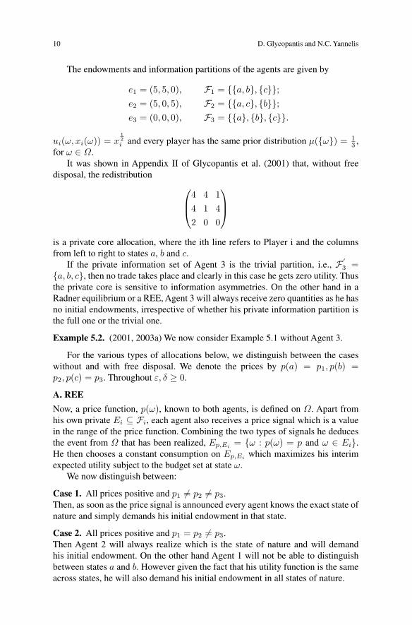
The endowments and information partitions of the agents are given by
e1 = (5, 5, 0), F1 = a, b, c;e2 = (5, 0, 5), F2 = a, c, b;e3 = (0, 0, 0), F3 = a, b, c.
ui(ω, xi(ω)) = x12i and every player has the same prior distribution µ(ω) = 1
3 ,for ω ∈ Ω.
It was shown in Appendix II of Glycopantis et al. (2001) that, without freedisposal, the redistribution ⎛⎜⎝4 4 1
4 1 42 0 0
⎞⎟⎠is a private core allocation, where the ith line refers to Player i and the columnsfrom left to right to states a, b and c.
If the private information set of Agent 3 is the trivial partition, i.e., F ′3 =
a, b, c, then no trade takes place and clearly in this case he gets zero utility. Thusthe private core is sensitive to information asymmetries. On the other hand in aRadner equilibrium or a REE, Agent 3 will always receive zero quantities as he hasno initial endowments, irrespective of whether his private information partition isthe full one or the trivial one.
Example 5.2. (2001, 2003a) We now consider Example 5.1 without Agent 3.
For the various types of allocations below, we distinguish between the caseswithout and with free disposal. We denote the prices by p(a) = p1, p(b) =p2, p(c) = p3. Throughout ε, δ ≥ 0.
A. REE
Now, a price function, p(ω), known to both agents, is defined on Ω. Apart fromhis own private Ei ⊆ Fi, each agent also receives a price signal which is a valuein the range of the price function. Combining the two types of signals he deducesthe event from Ω that has been realized, Ep,Ei
= ω : p(ω) = p and ω ∈ Ei.He then chooses a constant consumption on Ep,Ei which maximizes his interimexpected utility subject to the budget set at state ω.
We now distinguish between:
Case 1. All prices positive and p1 = p2 = p3.Then, as soon as the price signal is announced every agent knows the exact state ofnature and simply demands his initial endowment in that state.
Case 2. All prices positive and p1 = p2 = p3.Then Agent 2 will always realize which is the state of nature and will demandhis initial endowment. On the other hand Agent 1 will not be able to distinguishbetween states a and b. However given the fact that his utility function is the sameacross states, he will also demand his initial endowment in all states of nature.

Equilibrium concepts in differential information economies 11
Case 3. All prices positive and p1 = p3 = p2.This is identical to Case 2 with the roles of the two agents interchanged.
Case 4. The positive prices are constant onΩ and hence non-revealing. Each agentrelies exclusively on his private information and will demand in each state his initialendowment.In all cases the rational expectations price function can be any such that its range ofvalues is a positive vector and it will confirm the initial endowments as equilibriumallocation. Furthermore it makes no difference to the above reasoning whether freedisposal is allowed or not.
We can also argue in general that with one good per state and monotonic utilityfunctions, the measurability of the allocations implies that REE, fully revealing ornot, simply confirms the initial endowments.
B. Radner equilibrium
The measurability of allocations implies that we require consumptions x1(a) =x2(b) = x and x1(c) for Agent 1, and x2(a) = x2(c) = y and x2(b) for Agent 2.We can also write x = 5− ε, x1(c) = δ, y = 5− δ and x2(b) = ε.
We now consider,
Case 1. Without free disposalThere is no Radner equilibrium with prices in R3
+.
Case 2. With free disposal.The prices are p1 = 0, p2 = p3 > 0 and the allocation is(
4 4 14 1 4
)·
It corresponds to ε, δ = 1 which means that in state a each of the agents throwsaway one unit of the good.
C. WFC
The agents pool their information and therefore any feasible consumption vectorto either agent will be measurable. Hence we do not need to distinguish betweenfree disposal and non-free disposal. All WFC allocations will exhaust the resourcein each state of nature.
There are uncountably many such allocations, as for example(5 2.5 2.55 2.5 2.5
)·
This allocation is∨2
i=1 Fi-measurable and cannot be dominated by any coalitionof agents using their pooled information.
Referring back to Example 5.1 we can note that a private core allocation isnot necessarily a WFC allocation. For example the division (4, 4, 1), (4, 1, 4) and(2, 0, 0), to Agents 1, 2 and 3 respectively, is a private core but not a weak finecore allocation. The first two agents can get together, pool their information and do

12 D. Glycopantis and N.C. Yannelis
Æ
Æ
Figure 1
better. They can realize the WFC allocation, (5, 2.5, 2.5), (5, 2.5, 2.5) and (0, 0, 0)which does not belong to the private core because of lack of measurability.
D. Private core
Case 1. Without free disposal.No individual can increase his allocation and retain measurability. Therefore, inthis case the only allocation in the core is the initial endowments.
Case 2. With free disposal.Free disposal can take the form:(
5− ε 5− ε δ
5− δ ε 5− δ
)where ε, δ > 0.
The private core is the section of the curve (δ + 13 )(ε + 1
3 ) = 169 between the
indifference curves corresponding to U1 = 2012 and U2 = 20
12 . Notice that the
allocation (4 4 14 1 4
)corresponds to δ, ε = 1 and is in the private core. The private core and the Radnerequilibrium are shown in Figure 1.
E. WFV
Here we shall show that x1 = x2 = (5, 2.5, 2.5) is a weak fine value allocation.First we note that the “join” F1 ∨ F2 = abc. So every allocation isF1 ∨ F2-measurable and condition (i) of Definition 3.5 is satisfied. Condition (ii)is also immediately satisfied.
Equilibrium concepts in differential information economies 13
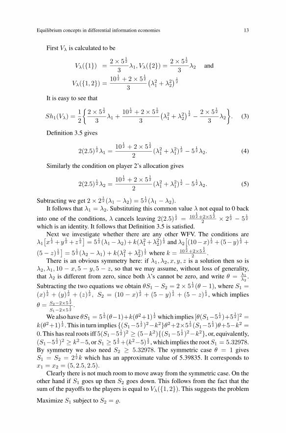
First Vλ is calculated to be
Vλ(1) =2× 5
12
3λ1, Vλ(2) =
2× 512
3λ2 and
Vλ(1, 2) =10
12 + 2× 5
12
3(λ2
1 + λ22) 1
2
It is easy to see that
Sh1(Vλ) =12
2× 5
12
3λ1 +
1012 + 2× 5
12
3(λ2
1 + λ22) 1
2 − 2× 512
3λ2
. (3)
Definition 3.5 gives
2(2.5)12λ1 =
1012 + 2× 5
12
2(λ2
1 + λ21)
12 − 5
12λ2. (4)
Similarly the condition on player 2’s allocation gives
2(2.5)12λ2 =
1012 + 2× 5
12
2(λ2
1 + λ21)
12 − 5
12λ2. (5)
Subtracting we get 2× 212 (λ1 − λ2) = 5
12 (λ1 − λ2).
It follows that λ1 = λ2. Substituting this common value λ not equal to 0 back
into one of the conditions, λ cancels leaving 2(2.5)12 = 10
12 +2×5
12
2 × 212 − 5
12
which is an identity. It follows that Definition 3.5 is satisfied.Next we investigate whether there are any other WFV. The conditions are
λ1[x
12 +y
12 +z
12]
= 512 (λ1−λ2)+k(λ2
1 +λ22)
12 and λ2
[(10−x) 1
2 +(5−y) 12 +
(5− z) 12]
= 512 (λ2 − λ1) + k(λ2
1 + λ22)
12 where k = 10
12 +2×5
12
2 .There is an obvious symmetry here: if λ1, λ2, x, y, z is a solution then so is
λ2, λ1, 10 − x, 5 − y, 5 − z, so that we may assume, without loss of generality,that λ2 is different from zero, since both λ’s cannot be zero, and write θ = λ1
λ2.
Subtracting the two equations we obtain θS1 − S2 = 2× 512 (θ − 1), where S1 =
(x)12 + (y)
12 + (z)
12 , S2 = (10 − x) 1
2 + (5 − y) 12 + (5 − z) 1
2 , which implies
θ = S2−2×512
S1−2×512.
We also have θS1 = 512 (θ−1)+k(θ2+1)
12 which implies [θ(S1−5
12 )+5
12 ]2 =
k(θ2+1)12 . This in turn implies (S1−5
12 )2−k2θ2+2×5
12 (S1−5
12 )θ+5−k2 =
0. This has real roots iff 5(S1−512 )2 ≥ (5−k2)(S1−5
12 )2−k2, or, equivalently,
(S1−512 )2 ≥ k2−5, orS1 ≥ 5
12 +(k2−5)
12 , which implies the rootS1 = 5.32978.
By symmetry we also need S2 ≥ 5.32978. The symmetric case θ = 1 givesS1 = S2 = 2
12 k which has an approximate value of 5.39835. It corresponds to
x1 = x2 = (5, 2.5, 2.5).Clearly there is not much room to move away from the symmetric case. On the
other hand if S1 goes up then S2 goes down. This follows from the fact that thesum of the payoffs to the players is equal to Vλ(1, 2). This suggests the problem
Maximize S1 subject to S2 = .
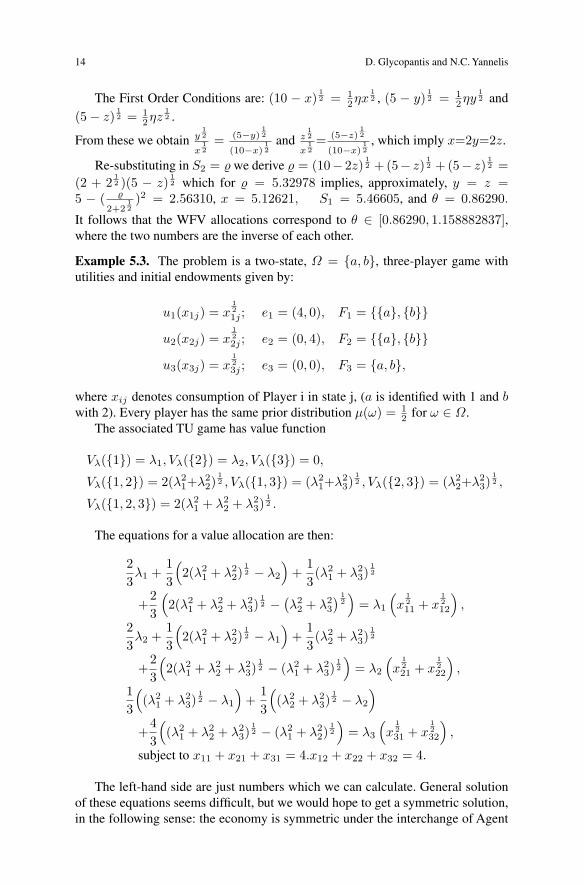
14 D. Glycopantis and N.C. Yannelis
The First Order Conditions are: (10 − x) 12 = 1
2ηx12 , (5 − y) 1
2 = 12ηy
12 and
(5− z) 12 = 1
2ηz12 .
From these we obtain y12
x12
= (5−y)12
(10−x)12
and z12
x12= (5−z)
12
(10−x)12
, which imply x=2y=2z.
Re-substituting in S2 = we derive = (10− 2z)12 +(5− z) 1
2 +(5− z) 12 =
(2 + 212 )(5 − z) 1
2 which for = 5.32978 implies, approximately, y = z =5 − (
2+212)2 = 2.56310, x = 5.12621, S1 = 5.46605, and θ = 0.86290.
It follows that the WFV allocations correspond to θ ∈ [0.86290, 1.158882837],where the two numbers are the inverse of each other.
Example 5.3. The problem is a two-state, Ω = a, b, three-player game withutilities and initial endowments given by:
u1(x1j) = x121j ; e1 = (4, 0), F1 = a, b
u2(x2j) = x122j ; e2 = (0, 4), F2 = a, b
u3(x3j) = x123j ; e3 = (0, 0), F3 = a, b,
where xij denotes consumption of Player i in state j, (a is identified with 1 and bwith 2). Every player has the same prior distribution µ(ω) = 1
2 for ω ∈ Ω.The associated TU game has value function
Vλ(1) = λ1, Vλ(2) = λ2, Vλ(3) = 0,
Vλ(1, 2) = 2(λ21+λ
22)
12 , Vλ(1, 3) = (λ2
1+λ23)
12 , Vλ(2, 3) = (λ2
2+λ23)
12 ,
Vλ(1, 2, 3) = 2(λ21 + λ2
2 + λ23)
12 .
The equations for a value allocation are then:
23λ1 +
13
(2(λ2
1 + λ22)
12 − λ2
)+
13(λ2
1 + λ23)
12
+23
(2(λ2
1 + λ22 + λ2
3)12 −(λ2
2 + λ23) 1
2)
= λ1
(x
1211 + x
1212
),
23λ2 +
13
(2(λ2
1 + λ22)
12 − λ1
)+
13(λ2
2 + λ23)
12
+23
(2(λ2
1 + λ22 + λ2
3)12 − (λ2
1 + λ23)
12
)= λ2
(x
1221 + x
1222
),
13
((λ2
1 + λ23)
12 − λ1
)+
13
((λ2
2 + λ23)
12 − λ2
)+
43
((λ2
1 + λ22 + λ2
3)12 − (λ2
1 + λ22)
12
)= λ3
(x
1231 + x
1232
),
subject to x11 + x21 + x31 = 4.x12 + x22 + x32 = 4.
The left-hand side are just numbers which we can calculate. General solutionof these equations seems difficult, but we would hope to get a symmetric solution,in the following sense: the economy is symmetric under the interchange of Agent

Equilibrium concepts in differential information economies 15
1 with Agent 2, together with interchange of the good in state 1 and the good instate 2; so we might expect a solution in which
x11 = x22, x12 = x21, x31 = x32, λ1 = λ2.
We will write, for simplicity
x1211 = x
1222 = x, x
1212 = x
1221 = y,
and hence x31 = x32 = (4− (x2 + y2))12 , λ1 = λ2 = λ.
We will treat two cases. Firstly, ifλ3 = 0, the last equation is identically satisfiedand the first two equations (which are the same) give 2 × 2
12λ = λ(x + y). So λ
is arbitrary and x + y = 2 × 212 . If we suppose x = 2
12 + δ, y = (−δ) 1
2 , thenx11 + x21 = 4 + δ2, so we have δ = 0 and hence
x11 = x12 = x21 = x22 = 2, x31 = x32 = 0,
with λ1 = λ2 > 0 arbitrary and λ3 = 0.Now consider the possibility that λ3 > 0 and we may normalise it to be equal
to 1. The first two equations are the same and they state:
13
(2(2)
12 + 1
)λ− 1
3(λ2 + 1)
12 +
43(2λ2 + 1)
12 = λ(x+ y). (6)
The third equation becomes
−23
(2(2)
12 + 1
)λ+
23(λ2 + 1)
12 +
43(2λ2 + 1)
12 = 2
[4− (x2 + y2)
] 12. (7)
It is a matter of tedious calculations on equations (16) and (17) to show thatthere are no value allocations with λ3 = 0 which are symmetric.
We now consider approximate equilibria, using the random algorithm. First welook into the case where in the equations for a value allocation we insertλi = 1, ∀i.The system does not perform very well. Approximate values can be found but thetotal error, the square root of the sum of squares of RHS-LHS of the equations, is0.21098557 which is rather large. On the other hand variations in the total resourceimprove the approximation.
If we allow in the system above for the λi’s also to be chosen then a rathersatisfactory approximate solution emerges:x11 = 1.9999, x12 = 2.0001, x21 = 2, 0000, x22 = 1.9998, x31 =
x32 = 0 (approximately), λ1 = 1, λ2 = 1.00009, λ3 = 0.0129, with total error0.000000007.
In the example we have examined Agent 3 has zero endowments and bad infor-mation. As a result, when all the λi’s can be chosen the solution of the equationsof the value allocation are approximately the same as when no weight is attachedto Agent 3.

16 D. Glycopantis and N.C. Yannelis
6 Two-good examples
We note that with one good per state and monotone utility functions there is a directrelation between allocations and utilities, i.e. x ≥ y iff u(x) ≥ u(y). This allowsone to prove results which do not hold in general. This is the reason why we presentalso examples with two goods. We also note that in the one good case the uniqueREE allocation exists always and it coincides with no trade. Thus it exists, it isincentive compatible and Pareto optimal. However, as it is shown below, this is notthe case when there are two goods.
Example 6.1. (2003b) We consider a two-agent economy, I = 1, 2 with twocommodities, i.e. Xi = R2
+ for each i, and three states of nature Ω = a, b, c.
The endowments, per state a, b, and c respectively, and information partitionsof the agents are given by
e1 = ((7, 1), (7, 1), (4, 1)), F1 = a, b, c;e2 = ((1, 10), (1, 7), (1, 7)), F2 = a, b, c.
We shall denote A1 = a, b, c1 = c, a2 = a, A2 = b, c.
ui(ω, xi1(ω), xi2(ω)) = x12i1x
12i2, and for all players µ(ω) = 1
3 , for ω ∈ Ω.We have that u1(7, 1) = 2.65, u1(4, 1) = 2, u2(1, 10) = 3.16, u2(1, 7) = 2.65and the expected utilities of the initial allocations, multiplied by 3, are given byU1 = 7.3 and U2 = 8.46.
A. REE
Case 1.First, we are looking for a fully revealing REE. Prices are normalized so that p1 = 1in each state. In effect we are analyzing an Edgeworth box economy per state.
State a. We find that
(p1, p2) =(
1,811
); x∗
11 =8522, x∗
12 =8516,
x∗21 =
9122, x∗
22 =9116
; u∗1 = 4.53, u∗
2 = 4.85.
State b. We find that
(p1, p2) = (1, 1); x∗11 = 4, x∗
12 = 4, x∗21 = 4, x∗
22 = 4; u∗1 = 4, u∗
2 = 4.
State c. We find that
(p1, p2) =(
1,58
); x∗
11 =3716, x∗
12 =3710, x∗
21 =4316,
x∗22 =
4310
; u∗1 = 2.93, u∗
2 = 3.40.
The normalized expected utilities of the equilibrium allocations are U1 =11.46, U2 = 12.25. This completes the analysis of the fully revealing REE.

Equilibrium concepts in differential information economies 17
We now look into whether there is a partially revealing or a non-revealing REEas well.
Case 2. Referring to the three states, we consider price vectors p1 = p2 = p3
or p1 = p2 = p3 or p1 = p3 = p2.We find that in all these cases no REE exists.
Case 3. We consider the price vectors to be equal, i.e. p1 = p2 = p3, which meansthat the Agents get no information from the prices.
We find that no such equilibrium exists.
The above analysis shows that there is only a fully revealing REE. The equilib-rium quantities are different in each state and therefore the REE allocations do notbelong to either the private core or Radner equilibria.
Next we characterize the Radner equilibria. Apart from the analysis in thecontext of Example 6.1, (Radner equilibria 1), we also consider a modified model,in Example 6.2, in which every agent can distinguish between all states of nature,(Radner equilibria 2). The calculations in the latter case can be contrasted to theones for the fully revealing equilibria.
Existence arguments in the case of correspondences can be advanced. Howeverthe actual calculation of such equilibria is not always straightforward.
B. Radner equilibria 1
The price vectors are p(a) = p1 = (p11, p12), p(b) = p2 = (p21, p
22) and p(c) =
p3 = (p31, p32). On the other hand we require measurability of allocations with
respect to the private information of the agents.The problems of the agents are:
Agent 1.Maximize U1 = 2(AB)
12 + (x3
11x312)
12
Subject to
A(p11 + p21) +B(p12 + p22) + p31x311 + p32x
312 = 7(p11 + p21) + (p12 + p22) + 4p31 + p32
and
Agent 2.Maximize U2 = (x1
21x122)
12 + 2(CD)
12
Subject to
p11x121 +p12x
122 +C(p21 +p31)+D(p22 +p32) = p11 +10p12 +(p21 +p31)+7(p22 +p32).
Applying a Gorman (1959) type argument we see that the demands of theagents will be of the form: A = M1
2(p11+p2
1), B = M1
2(p12+p2
2), x3
11 = M22p3
1, x3
12 = M22p3
2,
x121 = m1
2p11
, x122 = m1
2p12
, C = m22(p2
1+p31)
and D = m22(p2
2+p32)
.It follows that a Radner equilibrium with non-negative prices exists if the fol-
lowing system of equations has a non-negative solution.
2((p11 + p21)(p
12 + p22))
12
=1
(p31p32)
12,

18 D. Glycopantis and N.C. Yannelis
M1 +M2 = 7(p11 + p21) + (p12 + p22) + 4p31 + p321
(p11p12)
12
=2
((p21 + p31)(p22 + p32))
12
m1 +m2 = p11 + 10p12 + (p21 + p31) + 7(p22 + p32)M1
2(p11 + p21)+m1
2p11= 8,
M1
2(p12 + p22)+m1
2p12= 11
M2
2p31+
m2
2(p21 + p31)= 5,
M2
2p32+
m2
2(p22 + p32)= 8
M1
2(p11 + p21)+
m2
2(p21 + p31)= 8,
M1
2(p12 + p22)+
m2
2(p22 + p32)= 8.
The above system of equations is homogeneous of degree zero in the pij’s,
theMi’s and themi’s. Therefore some price, for example, p11 could be fixed whichreduces by one the number of unknowns. However the market equilibrium equationshave one degree of redundancy as a consequence of Walras’ law,
p11(A+ x121 − 8) + p12(B + x1
22 − 11) + p21(A+ C − 8) + p22(B +D − 8)+p31(x
311 + C − 5) + p32(x
312 +D − 8) = 0.
One can prove the existence of a Radner equilibrium by modifying the usualargument in general equilibrium theory, to take into account the fact that for Cobb-Douglas utility functions the demands are not defined on the whole boundary ofthe simplex. It is a rather tedious argument and we do not include it.
Approximate values for the equilibrium were obtained from the application ofthe random selection algorithm. A succession of random variables was appraisedusing a criterion consisting of the square root of the sum of squares of errors, thebest selection so far being retained at each step. We did not normalize prices andall equations were used.
We obtained p11 = 1.1566, p12 = 0.5876, p21 = 0.3979, p22 = 1.08597, p31 =1.3272, p32 = 0.49009, M1 = 14.1971, M2 = 4.1574, m1 = 7.9433, and m2 =11.8474, which satisfy the equations to three decimal places. We have also checkedthe accuracy to more decimal places. If an error implies infeasibility in the sensethat demand is larger than the resource then the implication is that a small quantityis not forthcoming. In the calculations we did not normalize prices, in order to allowfor the maximum flexibility in the algorithm.
The same approximate solution can be obtained using Newton’s method, start-ing the iteration from a suitable initial set of values. In order to avoid the problemsarising from the need to invert a singular matrix, we normalized p21 = 1 and,invoking Walras’ law, we left out the 4th market equilibrium equation.
However there are dangers which may be illustrated by leaving out the 6thmarket equation. For the same initial values we approach a different point, wherep22 is essentially zero but the sixth equation is not satisfied. This is possible becausein the Walras equation the contribution from the 6th equation has coefficient p22 andthus can take any value. This means that a particular limit point cannot be a Radnerequilibrium.
Equilibrium concepts in differential information economies 19
We also note that, of course, approximate solutions are not necessarily near thetrue solution. Even with continuity of functions the changes in the values corre-sponding to small changes in the variables might be very large.
We now have a digression the purpose of which is to explain that the fullinformation, deterministic Radner equilibrium is not the same as the fully revealingREE.
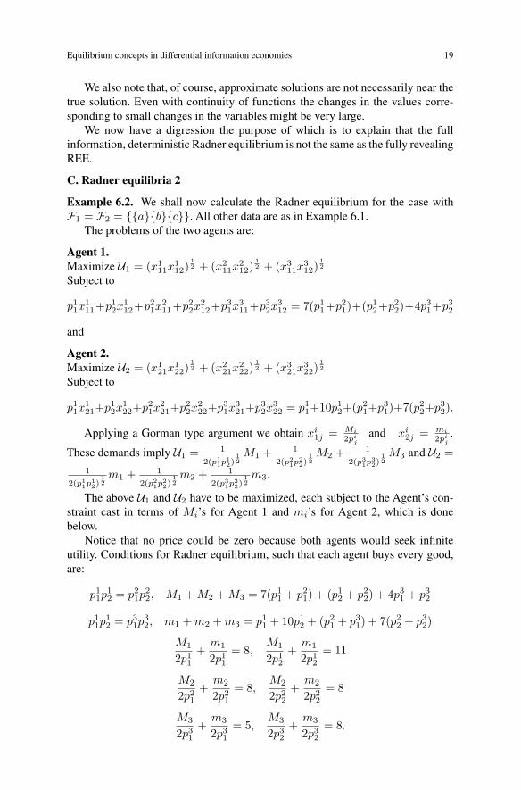
C. Radner equilibria 2
Example 6.2. We shall now calculate the Radner equilibrium for the case withF1 = F2 = abc.All other data are as in Example 6.1.
The problems of the two agents are:
Agent 1.Maximize U1 = (x1
11x112)
12 + (x2
11x212)
12 + (x3
11x312)
12
Subject to
p11x111+p12x
112+p21x
211+p22x
212+p31x
311+p32x
312 = 7(p11+p21)+(p12+p22)+4p31+p32
and
Agent 2.Maximize U2 = (x1
21x122)
12 + (x2
21x222)
12 + (x3
21x322)
12
Subject to
p11x121+p
12x
122+p
21x
221+p
22x
222+p
31x
321+p
32x
322 = p11+10p12+(p21+p
31)+7(p22+p
32).
Applying a Gorman type argument we obtain xi1j = Mi
2pij
and xi2j = mi
2pij.
These demands imply U1 = 12(p1
1p12)
12M1 + 1
2(p21p2
2)12M2 + 1
2(p31p3
2)12M3 and U2 =
12(p1
1p12)
12m1 + 1
2(p21p2
2)12m2 + 1
2(p31p3
2)12m3.
The above U1 and U2 have to be maximized, each subject to the Agent’s con-straint cast in terms of Mi’s for Agent 1 and mi’s for Agent 2, which is donebelow.
Notice that no price could be zero because both agents would seek infiniteutility. Conditions for Radner equilibrium, such that each agent buys every good,are:
p11p12 = p21p
22, M1 +M2 +M3 = 7(p11 + p21) + (p12 + p22) + 4p31 + p32
p11p12 = p31p
32, m1 +m2 +m3 = p11 + 10p12 + (p21 + p31) + 7(p22 + p32)
M1
2p11+m1
2p11= 8,
M1
2p12+m1
2p12= 11
M2
2p21+m2
2p21= 8,
M2
2p22+m2
2p22= 8
M3
2p31+m3
2p31= 5,
M3
2p32+m3
2p32= 8.

20 D. Glycopantis and N.C. Yannelis
The solution is obtained as follows: We normalize prices by setting p11 = 1.From the 5th and 6th equation we obtain p12 = 8
11 and the 7th and 8th equation implyp12 = p22. The 9th and 10th equation imply p32 = 5
8p31. Putting the last relations into
the 1st and 2nd we get the remaining prices. Putting all the information togetherwe have p11 = 1, p12 = 8
11 , p21 = p22 = ( 8
11 )12 , p31 = (64
55 )12 , and p32 = 5
8 × ( 6455 )
12 .
Employing the above values for pij we obtain for Mi and mi the following
relations:
M1 +M2 +M3 = 7× 811
+ 8×(
811
) 12
+ 458×(
6455
) 12
,
m1 +m2 +m3 = 838
+ 8×(
811
) 12
+ 538×(
6455
) 12
,
M1 +m1 = 16, M2 +m2 = 16×(
811
) 12
and M3 +m3 = 10×(
6455
) 12
,
which imply a possible solutionM1 = 7× 811 ,m1 = 8× 3
11 ,M2 = m2 = 8×( 811 )
12 ,
M3 = 4 58 × ( 64
55 )12 and m3 = 5 3
8 × ( 6455 )
12 . An obvious solution is M1 = 7 8
11 ,
m1 = 8 311 ,M2 = m2 = 8× ( 8
11 )12 ,M3 = 4 5
8 × ( 6411 )
12 andm3 = 5 3
8 × ( 6411 )
12 .
However this solution is not unique. For example, we can add to the value forM1 a small ε > 0 and subtract it fromm1, and then adjust in the opposite directionM2 andm2. We obtain then a new solution to the system with the same maximumvalue for the utilities.
It follows that the normalized prices for an interior solution are unique, andso are the maximum utilities, but the Mi’s and the mi’s can assume a number ofvalues. The explanation of the last observation is as follows. The product of thetwo goods to the power 1
2 becomes one good and given the equilibrium prices thestructure of the problem is such that the agents are as well off with ε > 0 as withε = 0.
One can ask why is it that the same argument would not apply to the previousformulation of Radner equilibria 1. There we seemed to be getting locally uniquevalues of Mi’s and mi’s. The reason was that we did not have the property thatrearranging incomes between the agents in Period 1 can be fully compensated bydoing so also in, for example, Period 2. In the present case the periods are amongthemselves separated. This was not the case in the previous formulation.
In that case, if we increase the composite commodity (AB)12 , where the Mi’s
have been calculated and decrease(x121x
122)
12 , by adjustingM1’s andm1’s, then we
have to decrease the commodity (x311x
312)
12 , and increase (CD)
12 , which requires
a reduction in (AB)12 . Everything was finally balanced there.
There are also approximate equilibria from the random algorithm, which ap-proach the true equilibrium above. Its application gives:
p11 = 1, p12 = 0.7272, p21 = 0.8528, p22 = 0.8528, p31 = 1.0787, p32 = 0.6742
and, approximately,M1 +m1 is 16.000051,M2 +m2 is 13.6448, andM3 +m3 is10.7871. The algorithm also captures the fact that the values of the Mi’s andmi’sare not fully determined.
Equilibrium concepts in differential information economies 21
On the basis of the above analysis, we see that full information Radner equilib-rium is not the same as fully revealing REE because in the latter case a monotonic,nonlinear transformation can be applied, such as replacing (xi
11xi12)
12 by (xi
11xi12),
without affecting the results as the calculations are per period. This is not the casein Radner equilibrium where the calculations are on the sum over all the periods.
We return now to the characterization of equilibrium concepts in Example 6.1.
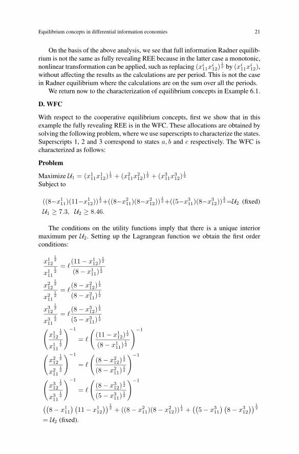
D. WFC
With respect to the cooperative equilibrium concepts, first we show that in thisexample the fully revealing REE is in the WFC. These allocations are obtained bysolving the following problem, where we use superscripts to characterize the states.Superscripts 1, 2 and 3 correspond to states a, b and c respectively. The WFC ischaracterized as follows:
Problem
Maximize U1 = (x111x
112)
12 + (x2
11x212)
12 + (x3
11x312)
12
Subject to
((8−x111)(11−x1
12))12 +((8−x2
11)(8−x212))
12 +((5−x3
11)(8−x312))
12 =U2 (fixed)
U1 ≥ 7.3, U2 ≥ 8.46.
The conditions on the utility functions imply that there is a unique interiormaximum per U2. Setting up the Lagrangean function we obtain the first orderconditions:
x112
12
x111
12
= (11− x1
12)12
(8− x111)
12
x212
12
x211
12
= (8− x2
12)12
(8− x211)
12
x312
12
x311
12
= (8− x3
12)12
(5− x311)
12(
x112
12
x111
12
)−1
=
((11− x1
12)12
(8− x111)
12
)−1
(x2
12
12
x211
12
)−1
=
((8− x2
12)12
(8− x211)
12
)−1
(x3
12
12
x311
12
)−1
=
((8− x3
12)12
(5− x311)
12
)−1
((8− x1
11) (
11− x112)) 1
2 + ((8− x211)(8− x2
12))12 +((
5− x311) (
8− x312)) 1
2
= U2 (fixed).
22 D. Glycopantis and N.C. Yannelis
It is easy to see that these conditions are satisfied by the REE allocations with theLagrange multiplier = 1.
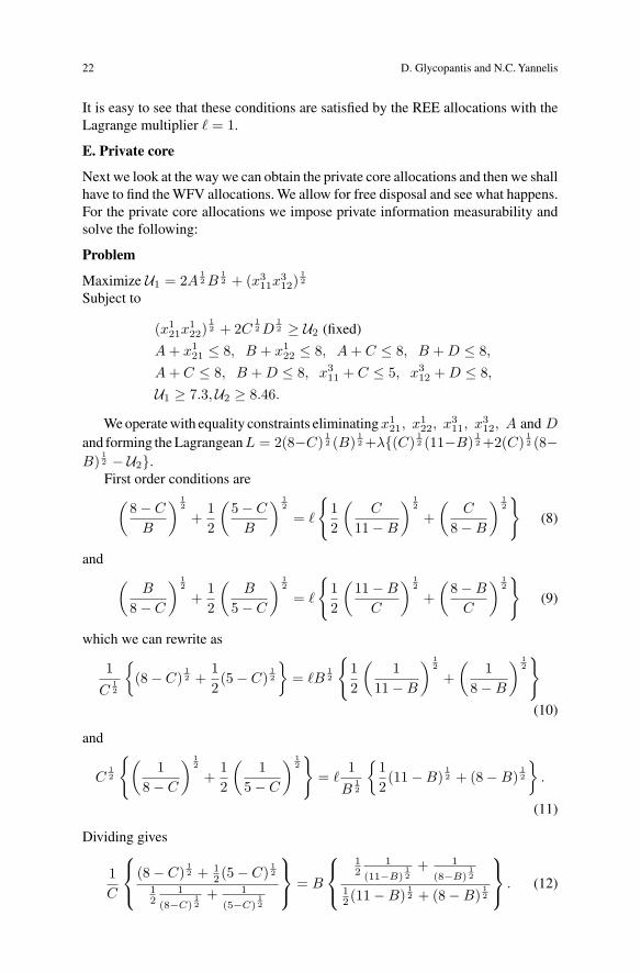
E. Private core
Next we look at the way we can obtain the private core allocations and then we shallhave to find the WFV allocations. We allow for free disposal and see what happens.For the private core allocations we impose private information measurability andsolve the following:
Problem
Maximize U1 = 2A12B
12 + (x3
11x312)
12
Subject to
(x121x
122)
12 + 2C
12D
12 ≥ U2 (fixed)
A+ x121 ≤ 8, B + x1
22 ≤ 8, A+ C ≤ 8, B +D ≤ 8,A+ C ≤ 8, B +D ≤ 8, x3
11 + C ≤ 5, x312 +D ≤ 8,
U1 ≥ 7.3,U2 ≥ 8.46.
We operate with equality constraints eliminatingx121, x
122, x
311, x
312, A and D
and forming the LagrangeanL = 2(8−C)12 (B)
12 +λ(C)
12 (11−B)
12 +2(C)
12 (8−
B)12 − U2.First order conditions are(
8− CB
) 12
+12
(5− CB
) 12
=
12
(C
11−B
) 12
+(
C
8−B
) 12
(8)
and (B
8− C
) 12
+12
(B
5− C
) 12
=
12
(11−BC
) 12
+(
8−BC
) 12
(9)
which we can rewrite as
1C
12
(8− C)
12 +
12(5− C)
12
= B
12
12
(1
11−B
) 12
+(
18−B
) 12(10)
and
C12
(1
8− C
) 12
+12
(1
5− C
) 12
= 1B
12
12(11−B)
12 + (8−B)
12
.
(11)
Dividing gives
1C
⎧⎨⎩ (8− C)12 + 1
2 (5− C)12
12
1(8−C)
12
+ 1(5−C)
12
⎫⎬⎭ = B
⎧⎨⎩12
1(11−B)
12
+ 1(8−B)
12
12 (11−B)
12 + (8−B)
12
⎫⎬⎭ . (12)

Equilibrium concepts in differential information economies 23
It is a matter of routine substitutions to show that the allocation x1 =((5.5, 5.5), (5.5, 5.5), (2.5, 5.5)), x2 = ((2.5, 5.5), (2.5, 2.5), (2.5, 2.5)) is inthe private core, with normalized expected utilities U1 = 14.70 and U2 = 8.70.
Next we show that this allocation cannot be obtained as a Radner equilibriumwith positive prices. We are looking for equality in all the conditions stated in thesection Radner equilibria 1. A corner solution would require some zero quantities.
Substituting into the conditions for the demand functions we obtain M1 =11(p11 + p21), m1 = 5p11, M1 = 11(p12 + p22), m1 = 11p12, M2 = 5p31, m2 =5(p11 + p21), M2 = 11p23 and m2 = (p22 + p32). We normalize and set p11 = 1.Then we obtain m1 = 5, p12 = 5
11 , p32 = 1, p31 = 115 , and we require further that
4p31p32 = (p11 + p21)(p
12 + p22) and 4p11p
12 = (p21 + p31)(p
22 + p32). These equations
cannot be satisfied by nonnegative prices because they imply−3.890 = 611p
21+
65p
22.
Obviously there are measurable allocations which are not in the private core,such as
x1 = ((5, 5), (5, 5), (2, 5)), and x2 = ((3, 6), (3, 3), (3, 3)),x1 = ((4, 4), (4, 4, (1, 4)), x2 = ((4, 7), (4, 4), (4, 4))
as can be seen through routine calculations.On the other hand we can show directly that a Radner equilibrium is in the
private core. Taking into account the constraints for demand to be equal to supply,the first order conditions for the agents’ maximization of utilities can be cast asfollows.
For Agent 1:
B12
(8− C)12− ′
(p11 + p21) = 0,(8− C)
12
B12
− ′(p12 + p22) = 0, (13)
12
B12
(5− C)12− ′
p31 = 0, and12
(5− C)12
B12
− ′p32 = 0, (14)
and for Agent 2:
12
(11−B)12
C12
− ψp11 = 0,12
C12
(11−B)12− ψp12 = 0, (15)
(8−B)12
C12
− ψ(p21 + p31) = 0, andC
12
(8−B)12− ψ(p22 + p32) = 0. (16)
Substituting (14), (15), (16) and (17) into (9) and (10) we obtain in both instancesthe relation
′= ψ which shows that the Radner equilibrium is in the private core.
F. WFV
Routine calculations imply Vλ(1) = 13λ1A, Vλ(2) = 1
3λ2B, where A =(2(7)
12 + 2) and B = (2(7)
12 + 10
12 ).
Next we have, Vλ(1, 2) = 13 maxx λ1(x1
11x112)
12 +λ2(8−x1
11)12 (11−x1
12)12 +
λ1(x211x
212)
12 +λ2(8−x2
11)12 (8−x2
12)12 +λ1(x3
11x312)
12 +λ2(5−x3
11)12 (8−x3
12)12 .

24 D. Glycopantis and N.C. Yannelis
We define the per period terms of the sum by U1, U2 and U3. We assume thatboth λ’s are positive. Otherwise all the weight is put on one agent. We can doseparate maximization and defining Λ1 = λ2
1, Λ2 = λ22 we obtain the conditions
(i) Λ1x112(8− x1
11) = Λ2x111(11− x1
12) and Λ1x111(11− x1
12) = Λ2x112(8− x1
11)(ii) Λ1x
212(8− x2
11) = Λ2x211(8− x1
12) and Λ1x211(8− x1
12) = Λ2x212(8− x2
11)(iii) Λ1x
312(5− x3
11) = Λ2x311(8− x3
12) and Λ1x311(11− x3
12) = Λ2x312(5− x3
11)
From (i), (ii) and (iii) we obtain, respectively, x112 = 11
8 x111, x2
12 = x211 and
x312 = 8
5x311. Which means that the maximum will be sought on these flats.
From the above we obtain U1 = ( 118 )
12 (λ1x
111 + λ2(8 − x1
11)), U2 =λ1x
211 + λ2(8 − x2
11)) and U3 = ( 85 )
12 (λ1x
311 + λ2(5 − x3
11)). It follows, that
Vλ(1, 2) = 13 maxx1 [(
118 )
12 (λ1x
111 + λ2(8− x1
11)) + (λ1x211 + λ2(8− x2
11)) +( 85 )
12 (λ1x
311 +λ2(5−x3
11))]. I.e. Vλ(1, 2) = 13 maxx1 [8(11
8 )12 max(λ1, λ2)+
8max(λ1, λ2) + 5(85 )
12 max(λ1, λ2)], which we can write as Vλ(1, 2) =
Cmax(λ1, λ2), where C = (88)12 + 8 + (40)
12 . The significance of the flats is
clear. For maximization the choice from the extreme values of the variable x1 de-pends on the values of λ1 and λ2. In particular for λ1 > λ2 all endowments areallocated to the utility function of Agent 1, for λ1 < λ2 the one of Agent 2, and forλ1 = λ2 the allocation can be arbitrary. This can be seen by obtaining Vλ(1, 2)through the per period maximization of the utility of Agent 1 subject to the utilityof Agent 2 being fixed.
For WFV allocations we require solutions to
λ1
∑ω
(x11(ω)x12(ω))12 =
12Cmaxλ1, λ2+Aλ1 −Bλ2 (17)
λ2
∑ω
(x21(ω)x22(ω)) =12Cmaxλ1, λ2 −Aλ1 +Bλ2
subject tox1 + x2 ≤ e1 + e2,
relaxing the feasibility condition. The right-hand sides of the equations above arethe Shi(Vλ)’s.
The set of WFV allocations is not empty. It can be checked that forλ1 = λ2 the allocation in which P1 gets ((4, 11
2 ), (5, 5), ( 54 , 2)) and P2 gets
((4, 112 ), (3, 3), ( 15
4 , 6)) is a WFV allocation. We see this by inserting these al-locations and λ1 = λ2 into the relations above to obtain
(22)12 + 5 + (2.5)
12 =
12
((88)
12 + 8 + (40)
12 + 2(7)
12 + 2− (10)
12 − 2(7)
12
)2((22)
12 + 3 + (7.5)
12 ) =
12
((88)
12 +8+(40)
12−2(7)
12−2+(10)
12 +2(7)
12
)which can be checked that they are satisfied.
On the other hand, it is a matter of tedious calculations to show that the fullyrevealing REE is not a WFV allocation although it belongs to the weak fine core.

Equilibrium concepts in differential information economies 25
Performing the calculations we obtain the relations
11.46λ1 =12[23.71max(λ1, λ2)+ 7.291λ1 − 8.45378λ2
]and
12.25λ2 =12[23.71max(λ1, λ2) − 7.291λ1 + 8.45378λ2
].
We distinguish between two cases and we examine whether the REE is in aweak fine value allocation.
Case 1. λ1 ≥ λ2We require
11.46λ1 =12[23.71λ1 + 7.291λ1 − 8.45378λ2
]and
12.25λ2 =12[23.71λ1 − 7.291λ1 + 8.45378λ2
]which imply 4.04λ1 = 4.23λ2 and 8.21λ1 = 8.22λ1 both of which cannot besatisfied.
Case 2. λ2 ≥ λ1We require now
22.92λ1 = 23.71λ2 + 7.291λ1 − 8.45378λ2 and
24.50λ2 = 23.71λ2 − 7.291λ1 + 8.45378λ2
which imply 15.63λ1 = 15.26λ2 and 7.66λ2 = 7.29λ1 which again cannot besatisfied.
The question arises why is the set of WFV allocations smaller than the WFC,although this of course is only true in the case of two agents.An intuitive explanationis that for the WFV allocations the conditions are more stringent because of thehomogeneity of equations in λ1, and λ2. We need to get from both equations in(18) the same λ1
λ2, and if we are given x(ω) this is highly unlikely to happen.
Now we show that a WFV equilibrium exists only for λ1 = λ2.Adding side by side the equations (18), we get on the RHS Cmaxλ1, λ2
which is equal to Vλ(1, 2). Therefore the sum on the LHS must be also equal toVλ(1, 2) and therefore a maximum, and we have seen how this depends on theweights λ1 and λ2.
Putting all the information together leads to the following possibilities. λ1 > λ2requires
λ1C =12
λ1C +Aλ1 −Bλ2
0 =
12λ1C −Aλ1 +Bλ2 .
Either of these leads toBλ2 = (A− C)λ1 < 0
which is impossible. Similarly λ1 < λ2 is impossible.

26 D. Glycopantis and N.C. Yannelis
Finally with λ1 = λ2 the equations for a weak-fine-value become, on writingyα = x12(ωα) and recalling that xα = 8
11yα,(811
) 12
(2y1 − 11) + (2y2 − 8) +(
58
) 12
(2y3 − 8) = 2− 1012
which is satisfied by the previous specified allocation.
Example 6.3. The problem is a two-state, Ω = a, b, three-player, two-goodgame with utilities and initial endowments given by:
u1(xj11, x
j12) = min(xj
11, xj12); e1 = ((1, 0), (1, 0)), F1 = a, b
u2(xj21, x
j22) = min(xj
21, xj22); e2 = ((0, 1), (0, 1)), F2 = a, b
u3(xj31, x
j32) =
xj31 + xj
32
2; e3 = ((0, 0), (0, 0)), F3 = a, b,
where xjik denotes consumption of Player i of Good k, in state j. Every player has
the same prior distribution µ(ω) = 12 for ω ∈ Ω.
The weights of the agents are λi for i = 1, 2, 3. First we calculate the charac-teristic function Vλ.
ForS = 1, 2 or 3we have ei = xi and so ui = 0. Therefore Vλ(i) =0. Next consider S = (1, 2). The sum of the weighted utilities∑
j∈Ω
12[λ1 min(xj
11, xj12) + λ2 min(xj
21, xj22)]
must be maximized subject to xj11 + xj
21 = 1 and xj12 + xj
22 = 1 for j ∈ Ω. It isstraightforward that for a maximum we must have x11 = x12 and x21 = x22 andthen that Vλ(1, 2) = max(λ1, λ2). It is also straigtforward that Vλ(1, 3) =Vλ(2, 3) = λ3
2 .We now turn our attention to S = 1, 2, 3. The expression
∑j∈Ω
12
[λ1 min(xj
11, xj12) + λ2 min(xj
21, xj22) + λ3
xj31 + xj
32
2
]
must be maximized subject to xj11 + xj
21 + xj31 = 1 xj
12 + xj22 + xj
32 = 1, forj ∈ Ω.
Again from the first two terms we get max(λ1, λ2) and for the whole constraintsum Vλ(1, 2, 3) = max(λ1, λ2, λ3).
Consider now the special case λi = 1 for i = 1, 2, 3. Replacing in the aboveλi by 1 we obtain
Vλ(i) = 0, for i = 1, 2, 3
Vλ(1, 2) = 1, Vλ(1, 3) = Vλ(2, 3) =12
for i = 2, 3
Vλ(1, 2, 3) = 1.

Equilibrium concepts in differential information economies 27
For this particular case, λi = 1, the Shapley values are given by
Sh1(V ) = 0 +16(1− 0) +
16
(12− 0)
+26
(1− 1
2
)=
512
Sh2(V ) =512, and Sh3(V ) =
212.
Hence the value allocation is, per state,
(x11, x12) = (x21, x22) =(
512,
512
)and (x31, x32) =
(212,
212
).
On the other hand any Walrasian type allocation will award zero quantities toPlayer 3, as he has no initial endowments. Therefore the point that this example ismaking is that with the number of agents n ≥ 3, it is possible that there is a valueallocation which does not belong to a Walrasian type set, (i.e. it is not a REE orRadner equilibrium).
However it can also be used to make one more point that is equally important.It can be seen that for λ1 = λ2 = 1 and λ3 = 0 or for the case where there isno third agent and with λ1 = λ2 = 1 we have Sh1(V ) = Sh2(V ) = 1
2 . This saysthat it is possible that a group which includes all the agents can do better for itsmembers than each one of them in isolation, but this is not the end of the story. Asub-group might do even better.
With respect to offering an interpretation of the distinction between side pay-ments and a WFV allocation, we look at the following situation. Two agents havesome initial endowments, the same weights, and their utilities are really revenuesfrom selling these quantities in a non-competitive market. We can hand over allquantities to one agent, ask him to sell them on the market, keep his Shapley shareand hand the other agent his own. With respect to the weak fine value it correspondsto the case when only a redistribution of the endowments is allowed, in which casewe might only be able to do it when specific weights are given to the individuals.
Non-existence of REE:Finally we discuss a specific version of the well known Kreps (1977) example of anon-existent REE. On the other hand, in the same example, the private core existswhich suggests that the latter concept has an advantage over that of REE.11
Example 6.4 (2003b). There are two agents I = 1, 2, two commodities, i.e.Xi = R2
+ for each Agent, i, and two states of nature Ω = ω1, ω2, considered bythe agents as equally probable. In xij the first index will refer to the agent and thesecond to the good.
We assume that the endowments, per state ω1 and ω2 respectively, and infor-mation partitions of the agents are given by
e1 = ((1.5, 1.5), (1.5, 1.5), F1 = ω1, ω2;e2 = ((1.5, 1.5), (1.5, 1.5), F2 = ω1, ω2.
11 Example 6.4 is also discussed in Glycopantis et al. (2003b).

28 D. Glycopantis and N.C. Yannelis
The utility functions of Agents 1 and 2 respectively, are for ω1 given by u1 =log x11 + x12 and u2 = 2 log x21 + x22 and for state ω2 by u1 = 2 log x11 + x12and u2 = log x21 + x22.
We consider first the possibility of REE.
Case 1. Fully revealing REE.Suppose that there exist, after normalization, prices (p1(1), p2(1))=(p1(2), p2(2)),where pi(j) denotes the price of good i in state j. The problems that the two agentssolve are as follows.
State ω1.
Agent 1:Maximize u1 = log x11 + x12Subject to
p1(1)x11 + p2(1)x12 = 1.5(p1(1) + p2(1))
and
Agent 2:Maximize u2 = 2 log x21 + x22Subject to
p1(1)x21 + p2(1)x22 = 1.5(p1(1) + p2(1)).
The agents solve analogous problems in state ω2. However it is not possibleto find (p1(1), p2(1)) = (p1(2), p2(2)). In the two problems the demands of theagents are interchanged so that the total demand stays the same while the totalsupply is fixed. It is also straightforward to check that there is no multiplicity ofequilibria per state.
Case 2. Non-revealing REE.Now we consider the possibility of p1(1) = p1(2) = p1 and p2(1) = p2(2) = p2.The two agents would act as follows.
Agent 1:He can tell the states of nature and obtains the demand functionsforω1,x11 = p2
p1andx12 = 1.5p1
p2+0.5 and forω2,x11 = 2p2
p1andx12 = 1.5p1
p2−0.5
for 3p1 ≥ p2.It is clear that the demands differ per state of nature.
Agent 2:He sets x21(ω1) = x21(ω2) = x21 and x22(ω1) = x22(ω2) = x22 and solves theproblem:
Maximize u2 = 12 (2 log x21 + x22) + 1
2 ( log x21 + x22) = 1.5 log x21 + x22Subject to
p1x21 + p2x22 = 1.5(p1 + p2).
So the highest indifference curve touches the budget constraint only once. Onthe other hand the demands of Agent 1 differ per ω. It follows that the marketscannot be cleared with common prices in both states of nature.
The above analysis shows that there is no REE in this model.

Equilibrium concepts in differential information economies 29
Next we consider, in the same example, the existence of private core allocations.These are obtained as solutions of the problem:
Maximize E2 = 1.5 log x21 + x22Subject to
12( log x11(ω1) + x12(ω1)) +
12( log x11(ω2) + x12(ω2)) ≥ E1 (fixed),
x1j(ω1), x1j(ω2) ≥ 0, E1, E2 ≥ 1.5 log 1.5 + 1.5x21 + x11(ω1) ≤ 3, x21 + x11(ω2) ≤ 3,x22 + x12(ω1) ≤ 3, x22 + x12(ω2) ≤ 3.
The structure of the problem, i.e. the continuity of the objective function and thecompactness of the feasible set, implies that it has always a solution. In particular,if we set the quantity constraints equal to 3 and 1.5 log 1.5 + 1.5 = E1 then theinitial allocation is in the private core.
The discussion of Example 6.4 indicates that the REE may not be an appropriateconcept to explain trades in DIE. The agents here receive no instructions as to whatthey should be doing.
7 Incentive compatibility
There are alternative formulations of the notion of incentive compatibility. Thebasic idea is that an allocation is incentive compatible if no coalition can misreportthe realized state of nature and have a distinct possibility of making its membersbetter off.
Suppose we have a coalition S, with members denoted by i, and the comple-mentary set I \ S with members j. Let the realized state of nature be ω∗. Eachmember i ∈ S sees Ei(ω∗). Obviously not all Ei(ω∗) need be the same, howeverall Agents i know that the actual state of nature could be ω∗.
Consider a state ω′
such that for all j ∈ I \ S we have ω′ ∈ Ej(ω∗) and for
at least one i ∈ S we have ω′/∈ Ei(ω∗). Now the coalition S decides that each
member i will announce that she has seen her own set Ei(ω′) which, of course,
contains a lie. On the other hand we have that ω′ ∈ ⋂j /∈S Ej(ω∗).
The idea is that if all members of I \S believe the statements of the members ofS then each i ∈ S expects to gain. For coalitional Bayesian incentive compatibility(CBIC) of an allocation we require that this is not possible. This is the incentivecompatibility condition we used in Glycopantis et al. (2001).12
We showed in Example 5.1 that in the three-agent economy without free disposalthe private core allocation x1 = (4, 4, 1), x2 = (4, 1, 4) and x3 = (2, 0, 0) isincentive compatible. This follows from the fact thatAgent 3 who would potentiallycheat in state a has no incentive to do so. It has been shown in Koutsougeras andYannelis (1993) that if the utility functions are monotone and continuous thenprivate core allocations are always CBIC.
12 See Krasa and Yannelis (1994) and Hahn and Yannelis (1997) for related concepts.

30 D. Glycopantis and N.C. Yannelis
On the other hand the WFC allocations are not always incentive compatible, asthe proposed redistribution x1 = x2 = (5, 2.5, 2.5) in Example 5.2 shows. Indeed,if Agent 1 observes a, b, he has an incentive to report c and Agent 2 has anincentive to report b when he observes a, c.
CBIC coincides in the case of a two-agent economy with the concept of Indi-vidually Bayesian Incentive Compatibility (IBIC), which refers to the case when Sis a singleton.
We consider here explicitly the concept of Transfer Coalitionally BayesianIncentive Compatible (TCBIC) allocations. This allows for transfers between themembers of a coalition, and is therefore a strengthening of the concept of Coali-tionally Bayesian Incentive Compatibility (CBIC).
Definition 7.1. An allocation x = (x1, . . . , xn) ∈ LX , with or without free dis-posal, is said to be TCBIC if it is not true that there exists a coalition S, states ω∗
and ω′, with ω∗ different from ω
′and ω
′ ∈ ⋂i/∈S Ei(ω∗) and a random, net-tradevector, z = (zi)i∈S among the members of S,
(zi)i∈S ,∑S
zi = 0
such that for all i ∈ S there exists Ei(ω∗) ⊆ Zi(ω∗) = Ei(ω∗)∩ (⋂
j /∈S Ej(ω∗)),for which ∑
ω∈Ei(ω∗)
ui(ω, ei(ω) + xi(ω′)− ei(ω
′) + zi)qi
(ω|Ei(ω∗)
)(18)
>∑
ω∈Ei(ω∗)
ui(ω, xi(ω))qi(ω|Ei(ω∗)
).
Notice that ei(ω) + xi(ω′)− ei(ω
′) + zi(ω) ∈ Xi(ω) is not necessarily mea-
surable. The definition implies that no coalition can hope that by misreporting astate, every member will become better off if they are believed by the members ofthe complementary set.
Returning to Definition 7.1, one can define CBIC to correspond to zi = 0 andthen IBIC to the case when S is a singleton. Thus we have (not IBCI)⇒ (not CBIC)⇒ (not TCBIC). It follows that TCBIC ⇒ CBIC ⇒ IBIC.
We now provide a characterization of TCBIC:
Proposition 7.1. Let E be a one-good DIE, and suppose each agent’s utility func-tion, ui = ui(ω, xi(ω)) is monotone in the elements of the vector of goodsxi, that ui(., xi) is Fi-measurable in the first argument, and that an elementx = (x1, . . . , xn) ∈ L1
X is a feasible allocation in the sense that∑n
i=1 xi(ω) =∑ni=1 ei(ω) ∀ω. Consider the following conditions:
(i) x ∈ L1X =
∏ni=1 L
1Xi
. and(ii) x is TCBIC.
Then (i) is equivalent to (ii).
Proof. See Glycopantis et al. (2003a).

Equilibrium concepts in differential information economies 31
Next we state conditions under which the private core allocation is CBIC.
Proposition 7.2. let E be an arbitrary differential information economy with mono-tone and continuous utility functions. The private core and the private value areCBIC.
Proof. See Koutsougeras and Yannelis (1993), Krasa and Yannelis (1994), andHahn and Yannelis (2001).
Corollary 7.1. A no-free disposal Radner equilibrium is CBIC.13
Proof. It can be easily shown that any no-free disposal Radner equilibrium be-longs to the private core. Therefore by Proposition 7.2 it follows that the Radnerequilibrium is CBIC.
Proposition 7.1 characterizes TCBIC and CBIC in terms of private individualmeasurability of allocations. It will enable us to conclude whether or not, in case ofnon-free disposal, any of the solution concepts will be TCBIC, whenever feasibleallocations are Fi-measurable.
It follows also that the redistribution(5 2.5 2.55 2.5 2.5
)is not CBIC because it is not Fi-measurable.
On the other hand the proposition implies, again in Example 5.1, that the allo-cation (
5 5 05 0 5
)is incentive compatible. As we have seen this is a non-free disposal REE, and aprivate core allocation.
We note that the above propositions are not true if we assume free disposal.In that case Fi-measurability does not imply incentive compatibility. In the casewith free disposal, private core and Radner equilibrium need not be incentivecompatible. In order to see this we notice that in Example 5.2 the (free disposal)Radner equilibrium is x1 = (4, 4, 1) and x2 = (4, 1, 4). The above allocation isclearly Fi-measurable and it can be checked directly that it belongs to the (freedisposal) private core. However it is not TBIC since if state a occurs Agent 1 hasan incentive to report state c and become better off.
Next we consider Example 6.1. We define A1 = a, b and A2 = b, c. Weassume that P1 acts first and that when P2 is to act he has heard the declarationof P1.
As shown in Section 6 the fully revealing REE allocations and correspondingutilities are:
In state a, x∗11 =
8522, x∗
12 =8516, x∗
21 =9122, x∗
22 =9116
;u∗1 = 4.53, u∗
2 = 4.85.
13 A direct proof of the CBIC of the non-free disposal Radner equilibrium with infinitely manycommodities has been given in Herves et al. (2003).

32 D. Glycopantis and N.C. Yannelis
In state b, x∗11 = 4, x∗
12 = 4, x∗21 = 4, x∗
22 = 4; u∗1 = 4, u∗
2 = 4.
In state c, x∗11 =
3716, x∗
12 =3710, x∗
21 =4316, x∗
22 =4310
;u∗1 = 2.93, u∗
2 = 3.40.
The normalized expected utilities of the REE are U1 = 11.46, U2 = 12.25.We can see that the REE redistribution, which belongs also to the WFC, is
not CBIC as follows.14 Suppose that P1 sees a, b and P2 seesa but misreportsb, c. If P1 believes the lie then state b is believed. So P1 agrees to get the allocation(4, 4). P2 receives the allocation e2(a)+x2(b)−e2(b) = (1, 10)+(4, 4)−(1, 7) =(4, 7) with u2(4, 7) = 5.29 > u2( 91
22 ,9116 ) = 4.85. Hence P2 has a possibility of
gaining by misreporting and therefore the REE is not CBIC. On the other hand ifP2 sees b, c and P1 sees c, the latter cannot misreport a, b and hope to gainif P2 believes it is b.
In employing game trees in the analysis we adopt the definition of IBIC. Thegame-theoretic equilibrium concept employed will be that of PBE. A play of thegame will be a directed path from the initial to a terminal node.
In terms of the game trees, a core allocation will be IBIC if there is a profile ofoptimal behavioral strategies along which no player misreports the state of naturehe has observed. This allows for the possibility that players have an incentive to liefrom information sets which are not visited by an optimal play.
In view of the analysis using game trees we comment further on the general ideaof CBIC. First we look at it again, in a similar manner to the one in the beginningof Section 4.
Suppose the true state of nature is ω. Any coalition can only see together thatthe state lies in
⋂i∈S Ei(ω). If they decide to lie they must first guess at what is
the true state and they will do so at some ω∗ ∈ ⋂i∈S Ei(ω). Having decided on
ω∗ as a possible true state, they pick some ω′ ∈ ⋂j /∈S Ej(ω∗) and assuming the
system is not CBIC they hope, by each of them announcingEi(ω′) to secure better
payoffs.This is all contingent on their being believed by I \ S, which depends on
having been correct in guessing that ω∗ = ω. If ω∗ = ω, i.e they guess wrongly,then since
⋂j /∈S Ej(ω∗) =
⋂j /∈S Ej(ω) the lie may be detected, since possibly
ω′/∈⋂
j /∈S Ej(ω).
Therefore the definition of CBIC can only be about situations where a lie mightbe beneficial. On the other hand the extensive form forces us to consider the al-ternative of what happens if the lie is detected. It requires statements concerningearlier decisions by other players to lie or tell the truth and what payoffs will occurwhenever a lie is detected, through observations or incompatibility of declarations.Only in this fuller description can players make a decision whether to risk a lie.Such considerations probably open the way to an incentive compatibility definitionbased on expected gains from lying.
The issue is whether cooperative and noncooperative static solutions can besupported through an appropriate noncooperative solution concept. The analysisbelow shows that CBIC allocations can be supported by a PBE while absence of
14 Palfrey and Srivastava (1986) have also shown that the REE may not be incentive compatible.

Equilibrium concepts in differential information economies 33
incentive compatibility implies lack of such support. It is also shown how imple-mentation of allocations becomes possible by introducing an exogenous third partyor an endogenous intermediary.
We recall that a PBE consists of a set of players’ optimal behavioral strategies,and consistent with these, a set of beliefs which attach a probability distributionto the nodes of each information set (Tirole, 1988). It is a variant of the idea of asequential equilibrium (Kreps and Wilson, 1982).
Note 7.1. Different notions of incentive compatibility for differential informationeconomies were first introduced by in Krasa andYannelis (1994). It should be notedthat the framework for differential information economies is different than the onein the Harsanyi type models and the notions of incentive compatibility which theyuse. These models assume that the initial endowments are independent of the stateof nature and therefore uncertainty comes only from the utility functions.
Notice that if the initial endowments are assumed to be constant, then mostof the examples in this paper cannot be analysed by a Harsanyi type model. Acomparison between the DIE model and the Harsanyi type models can be found inHahn and Yannelis (1997). In particular this paper contains a comparison of someof the Holmstrom and Myerson (1983) incentive compatibility notions and the onesin the DIE literature.
Finally it is important to notice that in a multilateral contracts model, it appearsmore appropriate to ensure CBIC rather than IBIC. Obviously CBIC implies IBICbut the reverse is not true, as an example in the preface of this volume demonstrates.Therefore lack of CBIC may make a contract unstable or not viable.
8 Non-implementation of Radner equilibria, of WFC and WFV allocations
We examine here the implementation, as a PBE of different equilibrium concepts.This section is closely related to the previous one. The fundamental issue is toconnect, in the context of the partition model, the idea of implementation, in theform of a PBE of an extensive form game, to the CBIC property. Namely, wewish to check whether an allocation can be realized as a PBE in an incompleteinformation, dynamic game, in the form of a tree, and how this is connected to theCBIC property.
The static concept of the CBIC implies that no agent has an incentive to liewith respect to the state(s) he has observed and the PBE satisfies basic rationalitycriteria in a game tree in which the agents are asymmetrically informed.
We examine whether cooperative or Walrasian, noncooperative, static equilib-rium allocations, can be supported as the outcome of a dynamic, noncooperativesolution concept. We also examine the role that a third party can play in supportingan equilibrium.
A general conclusion is that static equilibrium allocations with the CBIC prop-erty can be supported, under reasonable rules, as PBE outcomes. This discussion
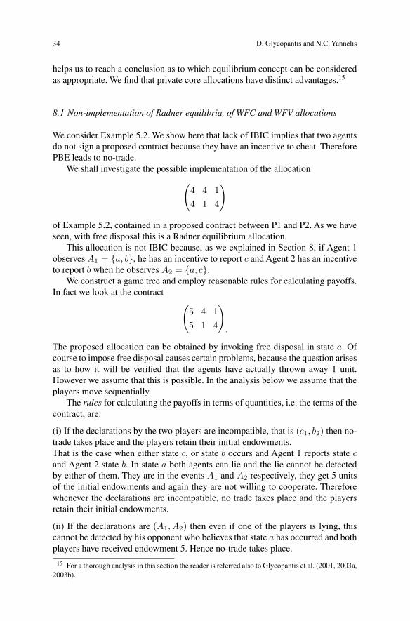
34 D. Glycopantis and N.C. Yannelis
helps us to reach a conclusion as to which equilibrium concept can be consideredas appropriate. We find that private core allocations have distinct advantages.15
8.1 Non-implementation of Radner equilibria, of WFC and WFV allocations
We consider Example 5.2. We show here that lack of IBIC implies that two agentsdo not sign a proposed contract because they have an incentive to cheat. ThereforePBE leads to no-trade.
We shall investigate the possible implementation of the allocation(4 4 14 1 4
)
of Example 5.2, contained in a proposed contract between P1 and P2. As we haveseen, with free disposal this is a Radner equilibrium allocation.
This allocation is not IBIC because, as we explained in Section 8, if Agent 1observes A1 = a, b, he has an incentive to report c and Agent 2 has an incentiveto report b when he observes A2 = a, c.
We construct a game tree and employ reasonable rules for calculating payoffs.In fact we look at the contract (
5 4 15 1 4
)·
The proposed allocation can be obtained by invoking free disposal in state a. Ofcourse to impose free disposal causes certain problems, because the question arisesas to how it will be verified that the agents have actually thrown away 1 unit.However we assume that this is possible. In the analysis below we assume that theplayers move sequentially.
The rules for calculating the payoffs in terms of quantities, i.e. the terms of thecontract, are:
(i) If the declarations by the two players are incompatible, that is (c1, b2) then no-trade takes place and the players retain their initial endowments.That is the case when either state c, or state b occurs and Agent 1 reports state cand Agent 2 state b. In state a both agents can lie and the lie cannot be detectedby either of them. They are in the events A1 and A2 respectively, they get 5 unitsof the initial endowments and again they are not willing to cooperate. Thereforewhenever the declarations are incompatible, no trade takes place and the playersretain their initial endowments.
(ii) If the declarations are (A1, A2) then even if one of the players is lying, thiscannot be detected by his opponent who believes that state a has occurred and bothplayers have received endowment 5. Hence no-trade takes place.
15 For a thorough analysis in this section the reader is referred also to Glycopantis et al. (2001, 2003a,2003b).

Equilibrium concepts in differential information economies 35
Figure 2
(iii) If the declarations are (A1, b2) then a lie can be beneficial and undetected. P1is trapped and must hand over one unit of his endowment to P2. Obviously if hisinitial endowment is zero then he has nothing to give.
(iv) If the declarations are (c1, A2) then again a lie can be beneficial and undetected.P2 is now trapped and must hand over one unit of his endowment to P1. Obviouslyif his initial endowment is zero then he has nothing to give.
For the calculations of payoffs the revelation of the actual state of nature is notrequired. We could specify that a player does not lie if he cannot get a higher payoffby doing so. We assume that each player, given his beliefs, chooses optimally fromhis information sets.
In Figure 2 we indicate, through heavy lines, plays of the game, obtained throughbackward induction, which are the outcome of the choices by nature and the optimalbehavioral strategies by the players. The interrupted lines signify that nature simplychooses among three alternatives, with equal probabilities. The fractions next tothe nodes of the information sets are obtained, whenever possible through Bayesianupdating. That is they are consistent with the choice of a state of nature and theoptimal behavioral strategies of the players.
For all choices by nature, at least one of the players tells a lie on the optimalplay. The players, by lying, avoid the possibility of having to make a payment andthe PBE confirms the initial endowments. The decisions to lie imply that the playerswill not sign the contract (5, 4, 1) and (5, 1, 4). A similar conclusion would havebeen reached if we investigated directly the allocation (4, 4, 1) and (4, 1, 4).

36 D. Glycopantis and N.C. Yannelis
Finally suppose we were to modify (iii) and (iv) of the rules i.e.: (iii) If the dec-larations are (A1, b2) then a lie can be beneficial and undetected, and P1 is trappedand must hand over half of his endowment to P2. Obviously if his endowment iszero then he has nothing to give.(iv) If the declarations are (c1, A2) then again a lie can be beneficial and undetected.P2 is now trapped and must hand over half of his endowment to P1. Obviously ifhis endowment is zero then he has nothing to give.
The new rules would imply the following changes in the payoffs in Figure 2,from left to right. The second vector would now be (2.5, 7.5), the third vector (7.5,2.5), the sixth vector (2.5, 2.5) and the eleventh vector (2.5, 2.5). The analysis inGlycopantis et al. (2001) shows that the weak fine core allocation in which bothagents receive (5, 2.5, 2.5) cannot be implemented as a PBE. Again this allocationis not IBIC. The same allocation belongs, for equal weights to the agents, also tothe WFV.
Finally we note that the PBE implements the initial endowments allocation(5 5 05 0 5
)
which in the case of non-free disposal, coincides with the REE. However as it isshown in Glycopantis et al. (2003b) a REE is not in general implementable.
8.2 Implementation of Radner equilibria and of WFC allocations through thecourts
We shall show briefly that the allocation(4 4 14 1 4
)of Example 5.2 can be implemented as a PBE through an exogenous third party.This can be interpreted as a court which imposes penalties when an agent lies.
Nature chooses states a, b and cwith equal probabilities. P1 acts first and cannotdistinguish between a and b. When P2 is to act we assume that not only he cannotdistinguish between a and c but also he does not know what P1 has chosen beforehim.
The rules are:
(i) If a player lies about his observation, then he is penalized by 1 unit of the good.If both players lie then they are both penalized. For example if the declarations are(c1, b2) and state a occurs both are penalized. If they choose (c1, A2) and state aoccurs then the first player is penalized. If a player lies and the other agent has apositive endowment then the court keeps the quantity subtracted for itself. However,if the other agent has no endowment, then the court transfers to him the one unitsubtracted from the one who lied.

Equilibrium concepts in differential information economies 37
Figure 3
(ii) If the declarations of the two agents are consistent, that is (A1, A2) and statea occurs, (A1, b2) and state b occurs, (c1, A2) and state c occurs, then they divideequally the total endowments in the economy.
We obtain through backward induction the equilibrium strategies by assumingthat each player chooses optimally, given his stated beliefs.
Figure 3 indicates, through heavy lines, optimal plays of the game. The fractionsnext to the nodes of the information sets are obtained through Bayesian updating.
Finally, suppose that the penalties are changed as follows. The court is extremelysevere when an agent lies while the other agent has no endowment. It takes all theendowment from the one who is lying and transfers it to the other player.
Now P2 will play A2 from I2 and P1 will play A1 from I1. Therefore invokingan exogenous agent implies that the PBE will now implement the WFC allocation
(5 2.5 2.55 2.5 2.5
)·

38 D. Glycopantis and N.C. Yannelis
Figure 4
8.3 Implementation of private core allocations
Here we draw upon the discussion in Glycopantis et al. (2001, 2003a). In the casewe consider now there is no court and therefore the agents in order to decide mustlisten to the choices of the other agents before them. P3 is one of the agents andwe investigate his role in the implementation of private core allocations. Again wedefine A1 = a, b and A2 = a, c.

Equilibrium concepts in differential information economies 39
Private core without free disposal seems to be the most satisfactory concept. Thethird agent, who has superior information, acting as an intermediary, implementsthe contract and gets rewarded in state a.
We shall consider the private core allocation⎛⎜⎝4 4 14 1 42 0 0
⎞⎟⎠of Example 5.1.
We know from Proposition 7.1 that such core allocations are CBIC and we shallshow now how they can be supported as PBE of a noncooperative game.
P1 cannot distinguish between states a and b and P2 between a and c. P3 seeson the screen the correct state and moves first. He can either announce exactly whathe saw or he can lie. Obviously he can lie in two ways. When P1 comes to decide hehas his information from the screen and also he knows what P3 has played. Whenit is the turn of P2 to decide he has his information from the screen and he alsoknows what P3 and P1 played before him. Both P1 and P2 can either tell the truthabout the information they received from the screen or they can lie.
The rules of calculating payoffs, i.e. the terms of the contract, are as follows:If P3 tells the truth we implement the redistribution in the matrix above which isproposed for this particular choice of nature.If P3 lies then we look into the strategies of P1 and P2 and decide as follows:
(i) If the declaration of P1 and P2 are incompatible we go to the initial endowmentsand each player keeps his.
(ii) If the declarations are compatible we expect the players to honour their commit-ments for the state in the overlap, using the endowments of the true state, providedthese are positive. If a player’s endowment is zero then no transfer from that agenttakes place as he has nothing to give.
In Figure 4 we indicate through heavy lines the equilibrium paths. The directedpaths (a, a,A1, A2) with payoffs (4, 4, 2), (b, b, A1, b2) with payoffs (4, 1, 0) and(c, c, c1, A2) with payoffs (1, 4, 0) occur, each, with probability 1
3 . It is clear thatnobody lies on the optimal paths and that the proposed reallocation is incentivecompatible and hence it will be realized.
Further we can show that the PBE in Figure 4 can also be obtained as a sequentialequilibrium in the sense of Kreps - Wilson (1982). Now, it is also required that theoptimal behavioral strategies, and the beliefs consistent with these, are the limit ofa sequence consisting of completely mixed behavioral strategies, and the impliedbeliefs. Throughout the sequence it is only required that beliefs are consistent withthe strategies. The latter are not expected to be optimal.
8.4 Non-implementation of REE
We show here, in the context of an economy with two agents, three states of natureand two goods per state, that a fully revealing REE is not implementable. In fact

40 D. Glycopantis and N.C. Yannelis
we consider Example 6.1. We recall that A1 = a, b, A2 = b, c, and assumethat P1 acts first and that when P2 is to act he has heard the declaration of P1. Wehave seen in Section 7 that the REE is not CBIC.
Next we show using the sequential decisions approach that the REE is notimplementable. We specify the rules for calculating payoffs, i.e. the terms of thecontract:
(i) If the declarations of the two players are incompatible, that is (c1, a2), then thisimplies that no trade takes place.
(ii) If the declarations of the two players are (A1, A2) then this implies that state bis believed. The player who believes it gets his REE allocation (4, 4) and the otherplayer gets the rest. So aA1A2 means that P2 has lied but P1 believes it is state band and gets (4, 4). P2 gets the rest under state a that is (4, 7); bA1A2 means thatboth believe that it is the (actual) state b and each gets (4, 4); cA1A2 means that P2believes it is state b and gets (4, 4) and P1 gains nothing from his lie as he gets (1,4).
(iii) aA1a2, bA1A2, cc1A2 imply that everybody tells the truth and the contractimplements the REE allocation under state a, b, and c respectively. (bA1A2 in (ii)and (iii) give of course an identical result).
(iv) ac1A2 implies that both lie but their declarations are not incompatible. Eachgets his REE under c and there is free disposal.
(v) cA1a2 means that both lie and stay with their initial endowments as they cannotget the REE allocations under state a which is the intersection of A1 and a2.
(vi) bA1a2 implies that P2 misreports and P1 believes and gets his REE under a;P2 gets the rest under b.
(vii) bc1A2 means that P1 lies and P2 believes that it is state c. P2 gets his REEallocation under c and P1 gets the rest under b, that is the allocation (5.31, 3.7).
On the game tree of consecutive decisions, the payoffs are translated in terms ofutility. The complete optimal paths are shown in Figure 5, through heavy lines. Weassume that each player chooses optimally from his information set. Probabilitiesnext to the nodes of the information sets denote the players’ beliefs. Strategies andbeliefs satisfy the condition of a PBE. Our analysis shows that it is unique16. Thecorresponding normalized expected payoffs of the players are U1 = 10.93 andU2 = 12.69.
The equilibrium paths imply that REE is not implementable which matchesup with the fact that it is not CBIC. However comparing the normalized expectedutilities of the Bayesian equilibrium with those corresponding to the initial alloca-tion we conclude that the proposed contract will be signed. On the other hand P2,because it is not advantageous to him, stops P1 from realizing his normalized REEutility. He ends up with U2 = 12.69 rather than U2 = 12.25.
Further, it is shown in Glycopantis et al. (2003b) that if we modify the model intoone with simultaneous decisions of the agents again the REE is not implementable.
16 Notice that as explained in the more detailed analysis, reversing the order of the play between theagents results in more than one PBE.

Equilibrium concepts in differential information economies 41
Figure 5
9 REE and weak core concepts
In view of the significance of the REE as an equlibrium concept we look in thissection closer at the relation between REE and weak core concepts, which allow forsharing of information among the agents.17 It is this sharing of information whichmakes the conditions different and therefore the comparison interesting, as REE isa Walrasian notion. The relation between REE and the private core, in which everyagent keeps their own information, has been examined above.
We show here that for state independent utilities, no coalition of agents can blocka fully revealing REE. Therefore in this case the REE is always a subset of IWFCand therefore it is interim “fully” Pareto optimal. However for state dependentutility functions the REE is not necessarily in the IWFC as we show below.
We also show that in general a REE does not belong to the WFC. If it so happensthat REE does belong to this set then a slight modification of the utility functionsimplies that the two sets do not overlap anymore.
9.1 REE and IWFC
First we define the cooperative concept of the IWFC concept which is conditionalon some information already obtained and shared by coalitions of agents.
17 This section uses results and statements from Glycopantis et al. (2003b).

42 D. Glycopantis and N.C. Yannelis
Definition 9.1.1. An allocation x = (x1, . . . , xn) ∈ LX is said to be a IWFCallocation if
(i) each xi(·) is FI -measurable;18
(ii)∑n
i=1 xi(ω) =∑n
i=1 ei(ω) for all ω ∈ Ω;(iii) there do not exist state of nature ω∗ ∈ Ω, coalition S and allocation
(yi)i∈S ∈∏
i∈S LXisuch that yi(·) − ei(·) is FS-measurable for all i ∈ S,∑
i∈S yi(ω) =∑
i∈S ei(ω), for all ω and vi(yi|FS)(ω∗) > vi(xi|Fxi)(ω∗)
for all i ∈ S, where Fxi denotes the information connected with xi.
The definition, (see Yannelis, 1991), implies that no coalitions of agents canpool their own information and make each of its members better off.
Proposition 9.1.1. For state independent utility functions, a fully revealing REEallocation belongs to the IWFC.
Proof. Let (x, p) be a fully revealing REE, so that the state of nature that hasoccurred is known to everybody and x be feasible and measurable with respect toFI . Suppose now that x is not an element of IWFC. Then there exists ω∗ ∈ Ω,a coalition S and feasible (yi)∈S ∈
∏i∈S LXi
which is FS-measurable ∀i ∈ S,such that
∑i∈S yi(ω) =
∑i∈S ei(ω) ∀ω ∈ Ω and
vi(yi|FS)(ω∗) > vi(xi|Gi)(ω∗). (19)
On the right-hand side of (6) we have thatGi = F which in this case is generatedby singletons.
We consider the two terms in relation to the Definition 9.1.1. The right-handside is vi(xi|Gi)(ω∗) = ui(xi(ω∗)), i.e. one single term with probability one. Thisfollows from the fact that x is fully revealing and therefore EGi
i (ω∗) = ω∗.On the other hand the left-hand side is
vi(ω∗, yi(ω∗)) =∑ω′ui(yi(ω′))qi(ω′|EFS
i (ω∗)), (20)
where in (7)
qi(ω′|EFSi (ω∗)) =
⎧⎪⎨⎪⎩0 : ω′ /∈ EFS
i (ω∗)
qi(ω′)qi(EFS
i (ω∗)): ω′ ∈ EFS
i (ω∗).
and EFSi (ω∗) is a subset of FS on which yi is constant.
This allows us to take the utility term out of the sum19 and deduce thatui(yi(ω∗)) > ui(xi(ω∗)). This implies that when xi was chosen yi was too expen-sive and therefore p(ω∗)yi(ω∗) > p(ω∗)xi(ω∗) = p(ω∗)ei(ω∗) ∀ i ∈ S. Thensumming up with respect to i ∈ S we obtain
p(ω∗)∑i∈S
yi(ω∗)=∑i∈S
p(ω∗)y(ω∗)>∑i∈S
pi(ω∗)ei(ω∗)=p(ω∗)∑i∈S
ei(ω∗). (21)
18 Recall that for S ⊆ I , FS denotes the “join" of coalition S, i.e.∨
i∈S Fi.19 Notice that if ui(ω′, xi(ω′)) depended separately on ω′ then, in general, it would not have been
possible to take ui(ω′, yi(ω′)) out of the sum. On the other hand measurability of ui with respect toits first argument would rescue the proof.

Equilibrium concepts in differential information economies 43
Relation (21) is a contradiction to∑
i∈S yi(ω) =∑
i∈S ei(ω) because in orderto obtain the inequality p(ω∗)
∑i∈S yi(ω∗) > p(ω∗)
∑i∈S ei(ω
∗) at least oneelement of the vector
∑i∈S yi(ω) must be larger than the corresponding element
of∑
i∈S ei(ω).
Remark 9.1.1. With state independent utilities, Proposition 9.1.1 can be proveneven if x is a partially revealing or non-revealing REE. It does not matter whetherthe information of the coalition is finer or not than the one of the REE. Also withstate dependent utilities the proposition can be proven for general REE and an ap-propriately defined WFC concept if coalitions are only allowed to form which havethe same information as REE. Then there is no need to take the utility expressionsout of the relation vi(yi|FS)(ω∗) > vi(xi|Gi)(ω∗). An interpretation of what theproposition implies is that, under certain conditions, allowing all possible coalitionsto share their information will not block the REE allocations.
Kwasnica (1998) has discussed a related result for a different core conceptwhich is not interim fully Pareto optimal.
The conditions under which Proposition 9.1.1 holds are limited. We now con-struct examples to show that it does not necessarily hold when we have state de-pendent utilities.
In the examples below the introduction ofAgent 3 is done so that the REE satisfy(i) in the definition of the IWFC. Alternatively, without introducing a third agentwe can argue that given a REE there exists an IWFC allocation which improves theconditional utility of an agent given some particular state.
Example 9.1.1. There are only two, equally probable, from the point of view ofthe agents, states of nature, (one can add more states to make the model richer butthis is not important), and two goods. Players 1 and 2 cannot distinguish betweenstates a and b. On the other hand their utility functions differ per state. Player 3 candistinguish between all states of nature, has no initial endowments and has someutility function. His role is to ensure that the vector x described below satisfiescondition (i) of IWFC. We turn our attention to the other players.
We are assuming the following. In state a: u1 = minεx11, x12, where ε > 1,and e1=(2, 0);u2= minx21, x22, and e2=(0, 2). In state b: u1= minx11, x12,and e1=(2, 0) u2=(x21x22)c, where c > 0 will be determined later, and e2 =(0, 2).
We construct two Edgeworth boxes and find the fully revealing REE, and henceour vectorx, to be as follows. In statea:p1 = 0, p2 = 1; Agent 1 gets zero quantitiesand Agent 2 gets everything; u1 = 0 and u2 = 2. In state b: p1 = 1, p2 = 1; everyagent gets 1 unit of each good; u1 = 1 and u2 = 1. In both states, Player 3 receivesno quantities.
We will now show that this REE is not in the IWFC. Since, when the two playersshare their information, they still cannot distinguish between the two states we stillrequire measurability of the feasible allocation to satisfy condition (iii) of IWFC.

44 D. Glycopantis and N.C. Yannelis
The proposed allocation is that Agent 1 gets y1(a) = y1(b) = (0.75, 0.75) andAgent 2 gets y2(a) = y2(b) = (1.25, 1.25). The utility levels are as follows. In statea: u1 = 0.75, and u2 = 1.25 and in state b: u1 = 0.75, u2 = (1.25× 1.25)c.
We choose state a for the condition (iii) of IWFC. For agent 1 we have thatv1(y1)(a) is larger than his REE utility which is zero. Also, for sufficiently largec, we have for agent 2 that v2(y2)(a) = (1
2 )1.25 + ( 12 )(1.25 × 1.25)c > u2 = 2
(REE utility under a).As for the alternative approach, without introducing a third agent we can argue
that, given a REE, there exists an IWFC allocation which does better for someagent. First we use the above yi allocation to show that it does better under a. Thenwe can argue that there exists an IWFC allocation which for some agent does evenbetter in terms of utility conditioned on state a.
Example 9.1.2 (2003b). There are two, equally probable, from the point of view ofthe agents, states Ω = a, b and three players I = 1, 2, 3. Player 3 can detectall states, but he has no initial endowments; his only role is to ensure that the xi
calculated below satisfy condition (i) of IWFC. Players 1 and 2 cannot distinguishbetween the states.
We are assuming that in state a: u1 = x211x12, u2 = x2
21x222, e1 = ( 9
13 ,913 ),
e2 = ( 413 ,
413 ), and in state b: u1 = x0.5
11 x12, u2 = x21x22, e1 = ( 913 ,
913 ), e2 =
( 413 ,
413 ).
The REE is given by p(a)=(8, 5), x1(a)=(0.75, 0.6), x2(a)=(0.25, 0.4), andp(b)=(5, 8), x1(b)=(0.6, 0.75), x2(b)=(0.4, 0.25).
In the IWFC definition chooseω∗=a, S=1, 2, y1(a)=y1(b)=(0.6, 0.8), andy2(a) = y2(b) = (0.4, 0.2).
Then v1(y1)(a)=0.454, u1(a, x1(a))=0.337, v2(y2)(a)=0.043, u2(a,x2(a))= 0.01.
9.2 REE and WFC
Next we consider the relation between REE and the WFC in the context of a moregeneral model than Example 6.1 which was considered above. We find that an REEallocation is not necessarily in the WFC.
Example 9.2.1 (2003b). For simplicity, we treat originally a case with two players,two goods and two states. We also assume, in the beginning, that the players are,in all states, endowed with strictly positive endowments of both goods and that forboth players all states are equally probable. We assume that all states, j ∈ Ω, aredistinguishable by the two players when they pool their information.
The normalized expected utility functions of the two players are U1 =∑j(x
j11)
α(xj12)
β and U2 =∑
j(xj21)
α(xj22)
β where α, β > 0. Namely we assumethat they have identical, state independent utility functions. These assumptions canbe relaxed. In summary, the result of the analysis is that in general the REE doesnot belong to the WFC.
The WFC allocations are characterized through the following problem:
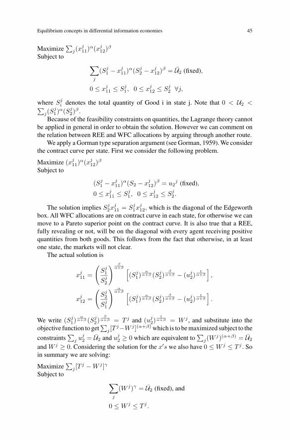
Equilibrium concepts in differential information economies 45
Maximize∑
j(xj11)
α(xj12)
β
Subject to ∑j
(Sj1 − xj
11)α(Sj
2 − xj12)
β = U2 (fixed),
0 ≤ xj11 ≤ Sj
1, 0 ≤ xj12 ≤ Sj
2 ∀j,
where Sji denotes the total quantity of Good i in state j. Note that 0 < U2 <∑
j(Sj1)
α(Sj2)
β .Because of the feasibility constraints on quantities, the Lagrange theory cannot
be applied in general in order to obtain the solution. However we can comment onthe relation between REE and WFC allocations by arguing through another route.
We apply a Gorman type separation argument (see Gorman, 1959). We considerthe contract curve per state. First we consider the following problem.
Maximize (xj11)
α(xj12)
β
Subject to
(Sj1 − xj
11)α(S2 − xj
12)β = u2
j (fixed),
0 ≤ xj11 ≤ Sj
1, 0 ≤ xj12 ≤ Sj
2.
The solution implies Sj2x
j11 = Sj
1xj12, which is the diagonal of the Edgeworth
box. All WFC allocations are on contract curve in each state, for otherwise we canmove to a Pareto superior point on the contract curve. It is also true that a REE,fully revealing or not, will be on the diagonal with every agent receiving positivequantities from both goods. This follows from the fact that otherwise, in at leastone state, the markets will not clear.
The actual solution is
xj11 =
(Sj
1
Sj2
) βα+β [
(Sj1)
αα+β (Sj
2)β
α+β − (uj2)
1α+β
],
xj12 =
(Sj
2
Sj1
) αα+β [
(Sj1)
αα+β (Sj
2)β
α+β − (uj2)
1α+β
].
We write (Sj1)
αα+β (Sj
2)β
α+β = T j and (uj2)
1α+β = W j , and substitute into the
objective function to get∑
j [Tj−W j ](α+β) which is to be maximized subject to the
constraints∑
j uj2 = U2 and uj
2 ≥ 0 which are equivalent to∑
j(Wj)(α+β) = U2
andW j ≥ 0. Considering the solution for the x′s we also have 0 ≤W j ≤ T j . Soin summary we are solving:
Maximize∑
j [Tj −W j ]γ
Subject to ∑j
(W j)γ = U2 (fixed), and
0 ≤W j ≤ T j .

46 D. Glycopantis and N.C. Yannelis
Figure 6
where γ = α+ β.
We now look at the form of the functions. Consider∑
j(Wj)γ = 1 for any
γ > 0.For γ = 1 this is a hyperplane. In the positive orthant, γ > 1 causes the surface tobulge away from the hyperplane so as to enclose a convex set including the origin(γ = 2 is the exemplary case, which is a hypersphere). Conversely for γ < 1 itproduces a surface which bulges in towards the origin.
∑j(W
j)γ = U2 is similar
in shape but scaled by a factor U1γ
2 .Finally the shape of
∑j [T
j−W j ]γ = K (fixed) can be derived from the above.The origin has been shifted to the point with coordinates (T j) after the surface hasbeen reflected along each coordinate axis.
Now we look at the solution of the overall Gorman problem. We distinguishbetween:
(i) γ > 1; the constraint is concave, in the nonnegative area, with perpendicularintersections with the axes. The indifference curves of the objective function areconvex, with nonnegative coordinates, (see Fig. 6), and increase in value as we

Equilibrium concepts in differential information economies 47
move in the direction of the origin. It follows that the maximum will be at one orboth of the corner points. This means that the REE is not in the WFC.
(ii) γ < 1; in this case the constraint is convex and the indifference curves areconcave, (see Fig. 6), and increase in value as we move in the direction of theorigin. The solution is away from the corner points at a point of tangency. Evenunder symmetric conditions there is no reason why the REE should be in the WFC.
(iii) γ = 1; inspection of the objective function and the constraint shows that theWFC coincides with the linear constraint. It follows that the REE allocation is inthe WFC and this is the case in Example 6.1. However, attaching a weight to theutility of Player 1 in one state implies a corner solution and therefore the REE isnot in the WFC.
10 Bayesian learning with cooperative solution concepts
As we indicated in the previous sections, the private core and the private valueoutcomes are sensitive to changes in the private information of the agents. In thissection we sketch out how information available to the agents can change throughtime.
The idea of learning introduces changes in the information structure of theagents. We consider a DIE that extends over many periods. The agents have ini-tially private information which reflects their own personal characteristics, i.e. therandom initial endowments and preferences. However, in each period they drawnew information from the realized core or value allocation. Hence we consider aneconomy E in a dynamic framework.
One way of explaining how the agents refine their private information over timeis as follows. Suppose, for example, that the same utility functions and endowmentsare repeated at each point in time. The chances are that over a long period all statesof nature will occur. Suppose now that Agent i knows exactly what this state is, saya, but Agent j observes an element of his information partition with more than onestate. Agent j cannot distinguish between the various states in his information set.However he can start slowly associating state a with signals which he originallyconsidered as unimportant or irrelevant and which now he sees coincide with theannouncement, through his private core or value allocation, of this state by Agenti. At no stage is it assumed that the agents get together to share their information.
Let T = 1, 2, ... denote the set of time periods and σ(eti, uti) the σ-algebra
that the random initial endowments and utility function of Agent i generated at timet. At any given point in time t ∈ T , the private information of Agent i is defined as:
F ti = σ(eti, u
ti, (x
t−1, xt−2, ...)) (22)
where xt−1, xt−2, ... are past periods private core or value allocations.Relation (22) says that at any given point in time t, the private information
which becomes available to Agent i is σ(eti, uti) together with the information
that the private core (value) allocations generated in all previous periods. In thisscenario, the private information of Agent i in period t+1 will beF t
i together with

48 D. Glycopantis and N.C. Yannelis
the information the private core (value) allocation generated at period t, i.e. σ(xt).More explicitly, the assumption is that the private information of Agent i at timet + 1 will be F t+1
i = F ti ∨ σ(xt), which denotes the "join", that is the smallest
σ-algebra containing F ti and σ(xt).
Therefore for each Agent i we have that
F ti ⊆ F t+1
i ⊆ F t+2i ⊆ ... . (23)
Relation (23) represents a learning process for Agent i and it generates a se-quence of differential information economies
Et : t ∈ T
where now the corre-
sponding private information sets are given by F ti : t ∈ T.
The agents are myopic, in the sense that they do not form expectations over theentire horizon but only for the current period, i.e. each agent’s interim expectedutility is based on his/her current period private information. Obviously, since theprivate information set of each agent becomes finer over time, the interim expectedutility of each agent is changing as well. The information gathered at a given timet, will affect the private core (or value) outcome in periods t + 1, t + 2, .... Theexample below attempts to explain the idea of learning.
Example 10.1. Consider the following DIE with two agents I = 1, 2 threestates of nature Ω = a, b, c and goods, in each state, the quantities of which aredenoted by xi1, xi2, where i refers to the agent. The utility functions are given by
ui(ω, xi1, xi2) = x12i1x
12i2, and states are equally probable, i.e. µ(ω) = 1
3 , forω ∈ Ω. Finally the measurable endowments and the private information of theagents is given by
et1 = ((10, 0), (10, 0), (0, 0)), F1 =a, b, c
;
et2 = ((10, 0), (0, 0), (10, 0)), F2 =a, c, b
. (24)
The structure of the private information of the agents implies that the private coreallocation, (xt
1, xt2), in t = 1 consists of the initial endowments.
Notice also that the information generated in Period 2 is the full informationσ(xt
1, xt2) =
a, b, c, a, b, a, c, a, b, c, ∅
. It follows that the private
information of each agent in periods t ≥ 2 will be
F t+11 = F t
1 ∨ σ(xt1, x
t2) =
a, b, c
;
F t+12 = F t
2 ∨ σ(xt1, x
t2) =
a, b, c
. (25)
Now in t = 2 the agents will make contracts on the basis of the private informationsets in (25). It is straightforward to show that a private core allocation in periodt ≥ 2 will be
xt+11 = ((5, 5), (10, 0), (0, 0));xt+1
2 = ((5, 5), (0, 0), (0, 10)). (26)
Notice that the allocation in (26) makes both agents better off than the one givenin (24). In other words, by refining their private information using the private coreallocation they have observed, the agents realized a Pareto improvement.

Equilibrium concepts in differential information economies 49
Of course, in a generalized model with more than two agents and a continuum ofstates, unlike the above example, there is no need that the full information privatecore or value will be reached in two periods. The main objective of learning isto examine the possible convergence of the private core or value in an infinitelyrepeated DIE. In particular, let us denote the one shot limit full information economyby E = (Xi, ui, Fi, ei, qi : i = 1, 2, ..., n) where Fi is the pooled informationof Agent i over the entire horizon, i.e. Fi =
∨∞i=1 F t
i .The questions that learning addresses itself to are the following:
(i) IfEt : t ∈ T
is a sequence of DIE and xt is a corresponding private core
or value allocation, can we extract a subsequence which converges to a limit fullinformation private core or value allocation for E?
(ii) Is the answer to (i) above affirmative, if we allow for bounded rationality inthe sense that xt is now required to be an approximate, ε-private core or ε-valueallocation for Et, but nonetheless it converges to an exact private core or valueallocation for E?
(iii) Given a limit full information private core or value allocation say x for E ,can we construct a sequence of ε-private core or ε-value allocation xt in Et whichconverges to x? In other words, can we construct a sequence of bounded rationalplays, such that the corresponding ε-private core or ε-value allocations converge tothe limit full information private core or value allocation.
The above questions have been affirmatively answered in Koutsougeras andYannelis (1999).
It should be noted that in the above framework it may be the case that in thelimit incomplete information may still prevail. In other words, it could be the casethat
Fi =∞∨
i=1
F ti ⊂
n∨i=1
F ti .
Hence in the limit a private core or value allocation may not be a fully revealingallocation of the same kind. However, if learning in each period reaches the completeinformation in the limit, i.e. Fi ⊃
∨ni=1 F t
i the private core or value allocation isindeed fully revealing.
Learning applied to cooperative solution concepts was first discussed in Kout-sougeras andYannelis (1999).A generalization of their results to non-myopic learn-ing which allows agents to discount the future can be found in Serfes (2001).
11 Concluding remarks
We have reviewed here relations between some of the main cooperative and non-cooperative equilibrium concepts in the area of finite economies with asymmetricinformation. It is precisely the asymmetry in the information of the agents whichleads to a variety of cooperative and noncooperative equilibrium concepts. It isthen appropriate that their properties be compared. As explained in Glycopantis

50 D. Glycopantis and N.C. Yannelis
and Yannelis in this volume, the example of Wilson (1978) shows that even the listof noncooperative concepts employed is not exhaustive.
Notice that we have not examined large economies or economies with infinitedimensional commodity spaces. There is a growing literature on such economies butwe decided to focus mainly on finite economies. This was for the sake of simplicity,and also for focusing on conceptual issues rather than proving powerful theorems.
In modeling a DIE, we followed the partition approach. Alternative conceptsare defined depending mainly on whether the calculations are in the ex ante orthe interim state, the degree of information sharing among the agents, the freedisposability or not of goods.
A number of examples calculate in detail equilibria, which makes their compari-son transparent. Relations are obtained and the significance of superior informationis brought out.
Given the variety of equilibrium concepts, the question arises which ones havesatisfactory properties. Two such properties are the static Bayesian incentive com-patibility and the dynamic PBE implementability of an equilibrium. We have alsoexhibited here some of the results obtained earlier which examined the connectionbetween these ideas.
The discussion considered both cooperative and Walrasian type equilibriumconcepts. The presentation here points out the positive association betweenBayesian incentive compatibility of a concept and its implementability as a PBE.This investigation is wider than the Nash (1953) programme which concentrates inproviding support to cooperative, static concepts through noncooperative, extensiveform constructions.
A main conclusion is that equilibrium notions which may not be incentivecompatible, cannot easily be supported as a PBE, e.g. REE and Radner equilibrium.On the contrary notions which are incentive compatible can be supported as a PBE,e.g. private core and private value.
We consider the area of incomplete and differential information and its mod-elling important for the development of economic theory. We believe that the intro-duction of game trees, which give a dynamic dimension to the analysis by makingthe individual decisions transparent, helps in the development of ideas. The parti-tion model is, in our view, a natural way to analyze DIE and the use of game treesprovides a noncooperative foundation of the equilibrium concepts.
Appendix I: On core concepts
We construct here a table containing a number of core concepts, taken as a startingpoint Yannelis (1991) and Koutsougeras and Yannelis (1993). We assume non-freedisposal and that the utility function with which comparisons will be made is theex ante one. First we cast the definition of a private core allocation in a form whichwill facilitate the comparison with other concepts.
Definition I.1. An allocation x(ω) = (x1(ω), x2(ω), ..., xn(ω)) with xi(ω) ∈Xi(ω) for all ω ∈ Ω and i = 1, ..., n, is a private core allocation if
(i) xi is Fi-measurable, for all i,

Equilibrium concepts in differential information economies 51
(ii)∑n
i=1 xi(ω) =∑n
i=1 ei(ω) for all ω, and(iii) there do not exist coalition S and allocation to S given by y(ω) =
(y1(ω), y2(ω), ..., yn(ω)) with yi(ω) ∈ Xi(ω) for al ω ∈ Ω and i ∈ Ssuch that(a) yi − ei is Fi-measurable for all i,(b)∑
i∈S yi(ω) =∑
i∈S ei(ω) for all ω, and(c) vi(yi) =
∑ω∈Ω ui(yi(ω))µ(ω) > vi(xi) =∑
ω∈Ω ui(yi(ω))ui(xi(ω))µ(ω) for i ∈ S.
We can now proceed to the following classification:
A1: If in (iii) (a) is replaced by∧
i∈S Fi-measurable20, it is a coarse core allocationA2: If also (i) is replaced by
∧i∈I Fi-measurable, it is a strong coarse core allo-
cationB1: If in (iii) (a) is replaced by
∨i∈S Fi-measurable, it is a fine core allocation
B2: If also (i) is replaced by∨
i∈I Fi-measurable, it is a a WFC allocation.
Therefore when we use the terms coarse or fine we are referring to the measur-ability of yi in (iii) (a). The terms strong or weak refer to the measurability of xi
in (i).Next we note that if F ⊆ G then x is F-measurable =⇒ x is G-measurable.
Thus if we make the σ-algebra in (i) finer, we make it easier to find a core element.Conversely, in (iii), where we ask that a certain function should not exist, makingthe σ-algebra coarser makes it easier to find a core element.
We note the relation between the sets, Fine Core (possibly ∅)⊆ Private Core⊆Coarse Core. The latter consists of individually rational Pareto optimal allocations.We also have that the strong coarse core is possibly empty, while the WFC exists.
We have that∧
i∈S Fi ⊆ Fi ⊆∨
i∈S Fi. Therefore, theoretically, we couldhave nine core concepts, shown in the table below.
(i)(iii) ∧ Fi Fi
∨ Fi∧ Fi Strong Coarse α βFi Coarse Private Fine∨ Fi γ δ Weak Fine
The set inclusion sign ⊇ applies in each row of the table from left to right, andin each column as we go down.
Note also that since WFC exists so do γ and δ. In the context of measurabilitythe private core concept is important. It has good properties: CBIC and it exists. Itis the smallest set which exists and is incentive compatible.
Obviously there are classifications as well, such as producing a table for freedisposal and one with interim utility functions. Some comparisons between entriesacross tables can be made.
20 The “meet” is the largest σ-algebra which is contained in each Fi. It is in a sense the intersectionof these algebras.

52 D. Glycopantis and N.C. Yannelis
It is of interest to make a comparison between Definition I.1 of the private coreabove, (Koutsougeras and Yannelis, 1993), and the definition below, (Yannelis,1991), which is cast in a positive formulation.
Definition I.2. An allocationx ∈ LX is said to be an interim private core allocation(IPC) if
(i)∑n
i=1 xi =∑n
i=1 ei and(ii) for all S and all (yi)i∈S ∈
∏i∈S LXi such that
∑i∈S yi =
∑i∈S ei, ∃i ∈ S
such that vi(ω, xi) ≥ vi(ω, yi) for some ω with µ(ω) > 0.
Despite the fact that in Definition I.2 interim expected utility functions wereused, one can show that IPC contains the ex ante private core in Definition I.1, i.e.PC⊆ IPC but not the other way round.
References
Allen, B.: Generic existence of completely revealing equilibria with uncertainty, when prices conveyinformation. Econometrica 49, 1173–1199 (1981)
Allen, B.: Market games with asymmetric information: the value. University of Pennsylvania, Workingpaper, 91-08 (1991a)
Allen, B.: Market games with asymmetric information and non-transferable utility: Representationresults and the core. University of Pennsylvania, Working paper, 91-09 (1991b)
Allen, B.: Incentives and market games with asymmetric information. Economic Theory 21, 527–544(2003)
Allen, B., Yannelis, N.C.: Differential information economies. Economic Theory 18, 263–273 (2001)Arrow, K.J., Debreu, G.: Existence of an equilibrium in a competitive economy. Econometrica 22,
265–290 (1954)Aumann, R.J.: Markets with a continuum of traders. Econometrica 32, 39–50 (1964)Aumann, R.J.: Correlated equilibria as an expression of Bayesian rationality. Econometrica 55, 1–18
(1987)Debreu, G.: Theory of value. New York: Wiley 1959Debreu, G., Scarf H.: A limit theorem on the core of an economy. International Economic Review 4,
235–246 (1963)Emmons, D., Scafuri, A.J.: Value allocations: an exposition. In: Aliprantis, C.D., Burkinshaw, O., Roth-
man, N.J. (eds): Advances in equilibrium theory. Lecture notes in economics and mathematicalsystems, pp. 55–78. Berlin Heidelberg New York: Springer 1985
Einy, E., Moreno, D., Shitovitz, B.: Rational expectations equilibria and the ex post core of an economywith asymmetric information. Journal of Mathematical Economics 34, 527–535 (2000)
Forges, F.: Le coeur d’une economie d’echange en information asymetrique. Mimeo (1998)Forges, F., Minelli, E., Vohra, R.: Incentives and the core of an exchange economy: a survey. Mimeo
(2000)Glycopantis, D., Muir,A.,Yannelis, N.C.:An extensive form interpretation of the private core. Economic
Theory 18, 293–319 (2001)Glycopantis, D., Muir, A.,Yannelis, N.C.: On extensive form implementation of contracts in differential
information economies. Economic Theory 21, 495–526 (2003a)Glycopantis, D., Muir, A., Yannelis, N.C.: Non-implementation of rational expectations as a perfect
Bayesian equilibrium. Mimeo (2003b)Glycopantis, A., Yannelis, N.C.: Information, efficiency and the core of the economy: Comments on
Wilson’s paper. This volume.Gorman, W.M.: Separable utility and aggregation. Econometrica 27, 469–481 (1959)Grossman, S.J.: An introduction to the theory of rational expectations under asymmetric information
economies. Review of Economic Studies 48, 541–560 (1981)
Equilibrium concepts in differential information economies 53
Hahn, G., Yannelis, N.C.: Efficiency and incentive compatibility in differential information economies.Economic Theory 10, 383–411 (1997)
Hahn, G., Yannelis, N.C.: Coalitional Bayesian Nash implementation in differential informationeconomies. Economic Theory 18, 485–509 (2001)
Harsanyi, J.C.: Games with incomplete information played by ‘Bayesian’ players, Part I. ManagementScience 14, 159–182 (1967)
Herves, C., Moreno, E.,Yannelis, N.C.: Equivalence and incentive compatibility of the Walrasian expec-tations equilibrium in infinite dimensional commodity spaces. Mimeo (2003). Economic Theory(forthcoming)
Hildenbrand, W.: Core and equilibria in large economies. Princeton, NJ: Princeton University Press1974
Holmstrom, B., Myerson, R.: Efficient and durable decision rules with incomplete information. Econo-metrica 51, 1799–1819 (1983)
Ichiishi, T.,Yamazaki, A.: Preliminary results for cooperative extensions of the Bayesian game. Discus-sion paper , Graduate School of Economics, Hitotsubashi University, 1-89 (2001-2)
Khan, M.A., Yannelis, N.C. (eds): Equilibrium theory in infinite dimensional spaces, pp. 233–248.Berlin Heidelberg New York: Springer 1991
Koutsougeras, L., Yannelis, N.C.: Incentive compatibility and information superiority of the core of aneconomy with differential information. Economic Theory 3, 195–216 (1993)
Koutsougeras, L.,Yannelis, N.C.: Bounded rational learning in differential information economies: Coreand value. Journal of Mathematical Economics 31, 373–391 (1999)
Krasa, S., Yannelis, N.C.: The value allocation of an economy with differential information. Economet-rica 62, 881–900 (1994)
Krasa, S.,Yannelis, N.C.: Existence and properties of a value allocation for an economy with differentialinformation. Journal of Mathematical Economics 25, 165–179 (1996)
Kreps, M.D.:A note on ‘fulfilled expectations’equilibria. Journal of Economic Theory 14, 32–43 (1977)Kreps, M.D., Wilson, R.: Sequential equilibrium. Econometrica 50, 889–904 (1982)Kwasnica,A.M.: Welfare properties of rational expectations equilibria: The core. Mimeo. Caltech (1998)Laffont, J.- J.: On the welfare analysis of rational expectation with asymmetric information. Economet-
rica 53, 1–29 (1985)Lefebvre, I.: An alternative proof of the nonemptiness of the private core. Journal of Economic Theory
14, 275–291 (2001)McKenzie, L.W.: On equilibrium in Graham’s model of world trade and other competitive systems.
Econometrica 22, 147–161 (1954)Myerson, R.: Cooperative games with incomplete information. International Journal of Game Theory
13, 69–96 (1982)Nash, J.F.: Two-person cooperative games. Econometrica 21, 128–140 (1953)Palfrey, T.R., Srivastava, S.: Private information in large economies. Journal of Economic Theory 39,
34–58 (1986)Prescott, E., Townsend, R.: Pareto optima and competitive equilibria with adverse selection and moral
hazard. Econometrica 52, 21–45 (1984)Radner, R.: Competitive equilibrium under uncertainty. Econometrica 36, 31–58 (1968)Radner, R.: Rational expectation equilibrium: generic existence and information revealed by prices.
Econometrica 47, 655–678 (1979)Scafuri, A.J., Yannelis, N.C.: Non-symmetric cardinal value allocations. Econometrica 52, 1365–1368
(1984)Serfes, K.: Non-myopic learning in differential information economies: the core. Economic Theory 18,
333–348 (2001)Shapley, L.S.: A value for n-person games. In: Kuhn, H.W., Tucker, A.W. (eds) Contributions to the
theory of games, II. Princeton: Princeton University Press 1953. Annals of Mathematical Studies28, 307–317 (1953)
Srivastava, S.: A limit theorem in the core with differential information. Economic Letters 14, 111–116(1984)
Tirole, J.: The theory of industrial organization. Cambridge, MA, London, UK: The MIT Press 1988Wilson, R.: Information, efficiency, and the core of an economy. Econometrica 46, 807–816 (1978)Yannelis, N.C.: The core of an economy with differential information. Economic Theory 1, 183–198
(1991)

PART 1
CORE NOTIONS, EXISTENCE RESULTS