equilibrium and kinetic studies in adsorption of toxic ... · photographic industries and painting,...
TRANSCRIPT

In: A Book on Ion Exchange, Adsorption and Solvent Extraction ISBN: 978-1-62417-887-0
Editors: Mu. Naushad and Zeid A. ALOthman © 2013 Nova Science Publishers, Inc.
Chapter 8
EQUILIBRIUM AND KINETIC STUDIES
IN ADSORPTION OF TOXIC METAL IONS
FOR WASTEWATER TREATMENT
Vicente de Oliveira Sousa Neto1, Giselle Santiago Cabral Raulino
2,
Paulo de Tarso C. Freire3, Marcos Antônio Araújo-Silva
3
and Ronaldo Ferreira do Nascimento4
1Department of Chemistry, State University of Ceará
(UECE-CECITEC), Brazil 2Department of Hydraulic and Environmental Engineering,
Federal University of Ceará (UFC), Brazil 3Department of Physical-Federal University of Ceará (UFC), Brazil
4Department of Analytical Chemistry and Physical Chemistry,
Federal University of Ceará (UFC), Brazil
ABSTRACT
In this chapter, applications are provided for batch and fixed-bed column adsorption
processes using coconut bagasse, an economic, effective, and efficient material for metal
ion removal from wastewater.
Investigations of the parameters that influence the performance of metal ion
adsorption, such as, effect of initial metal ion concentration, pH, flowrate, bed height, and
adsorption isotherm have been studied for selecting the most suitable treatment of
wastewater. Modeling of adsorption isotherm (Langmuir, Freudlich, Temkin, and Halsey
equations), adsorption kinetics (pseudo-first, pseudo-second and intraparticle equations)
and breakthrough curves (Thomas equation) were also applied to the experimental data to
find a better application and performance of the bio-adsorbent on the metal ion removal.
Corresponding author email address; [email protected]
No part of this digital document may be reproduced, stored in a retrieval system or transmitted commercially in any form or by any means. The publisher has taken reasonable care in the preparation of this digital document, but makes no expressed or implied warranty of any kind and assumes no responsibility for any errors or omissions. No liability is assumed for incidental or consequential damages in connection with or arising out of information contained herein. This digital document is sold with the clear understanding that the publisher is not engaged in rendering legal, medical or any other professional services.
V. de Oliveira Sousa Neto, G. S. C. Raulino, P. de Tarso C. Freire et al. 146
1. INTRODUCTION
The water contamination by toxic metals through the discharge of industrial wastewaters
is a worldwide environmental problem. The industries responsible for the discharge of
wastewaters containing metals are mining and mineral processing, pigment manufacture,
photographic industries and painting, metalworking, electroplating and finishing processes.
Since metals are non-biodegradable and may be bio-accumulated in living tissues, their
removal from wastewaters is nowadays legally imposed [1].
Conventional methods for removing metals from industrial effluents include coagulation,
chemical precipitation, solvent extraction, electrolysis, membrane separation ion exchange
and adsorption [2-6]. Even though these methods are efficient, some of them have limited
applications. Precipitation processes generate large quantities of sludge, which needs further
treatment and disposal. The high operational costs, particularly due to the high energy
consumption associated with electrolytic and membrane processes, limit their use, moreover
the secondary wastes generated are sometimes difficult to treat.
In recent years, considerations of public health, environmental and economic pressure
have made it desirable to reconsider the methods employed for treatment and disposal of toxic
wastes. From the waste generated, it is possible to highlight the toxic metals such as copper,
nickel and zinc. These metal ions are not degradable and can accumulate in the environment
where components manifest their toxicity and are movable. It can be very difficult to follow
the destination of these metal species in the ecosystem [7,8].
The high prices and regeneration cost of these materials limit their large-scale use for
metal ion removal. Thus, it has encouraged researchers to look for low cost sorbing materials
[8]. Attention has been focused on the various adsorbents, which have metal-binding
capacities and are able to remove unwanted heavy metals from contaminated water at low
cost [8]. Because of their low cost and local availability, natural materials such as zeolites and
clay, or certain waste products from industrial operations such as fly ash, coal, and oxides are
classified as low-cost adsorbents. The potential use of these residues as adsorbent materials
has two advantages, the reuse and its low cost. They can be disposed of without cost.
Among the numerous techniques of toxic metal removal, adsorption is the procedure of
choice and gives the best results because it can be used to remove different types of metal
species. The adsorption process has proven to be an excellent way to treat industrial effluents,
offering significant advantages like low-cost, availability, ease of operation and efficiency in
comparison with conventional methods especially from economical and environmental
viewpoints [7, 8].
2. ADSORPTION PROCESS
Adsorption can be defined as the accumulation of substances or materials at the interface
between a solid surface and solution. The adsorbing surface is the adsorbent, and the material
concentrated or adsorbed at the surface is the adsorbate (Figure 1). The adsorption process
involves a solid phase (sorbent or bio-sorbent; biological material) and a liquid phase
(solvent, normally water) containing a dissolved species to be adsorbed (i.e. adsorbate, metal
ions) [9,10,11].

Equilibrium and Kinetic Studies in Adsorption of Toxic Metal Ions ... 147
Due to a higher adsorbent affinity for the adsorbate species, the latter is attracted and
removed by different mechanisms. The adsorption process at equilibrium is established
between the amount of solid-bound adsorbate species and its portion remaining in the
solution. The degree of sorbent affinity for the adsorbate determines its distribution between
the solid and liquid phases.
2.1. Classification of Adsorption
According to the nature of the interaction between adsorbate and adsorbent, there are two
types of adsorption; physisorption and chemisorptions. The physisorption interaction is
relatively non-specific and is due to the operation of weak forces between species. In this
process, the adsorbed molecule is not affixed to a particular site on the solid surface; it is free
to move over the surface [12].
Figure 1. Adsorption process scheme of a surface.
Table 1. Properties of physisorption and chemisorption
Chemisorption Physisorption Reference
Monolayer adsorption Multilayer adsorption
[11,12,13]
High degree of specificity. Depends on the
number of actives sites
Low degree of specificity
High values to enthalpy of chemisorption Low values to enthalpy of
chemisorption
Endothermic or Exothermic Exothermic

V. de Oliveira Sousa Neto, G. S. C. Raulino, P. de Tarso C. Freire et al. 148
The physical interactions among species, based on electrostatic forces, include Vander
Waals interactions, dispersion interactions and hydrogen bonding. On the other hand,
chemisorption involves the formation of chemical bonds with the adsorbate being chemically
changed [12, 13-15]. Chemisorption is also based on electrostatic forces, but much stronger
forces play a major role in this process. In chemisorption, the attraction between adsorbent
and adsorbate is a covalent or ionic bond between atoms, with shorter bond length and higher
bond energy [13-15]. The differences between chemisorption and physisorption are given in
Table 1.
2.2. Interface Chemical Study
The ions interaction in the hydrosphere with solid components is subject to various types
of factors related to water properties such as temperature and pH.
It is very impressive to observe the growing number of papers reporting on applications
of adsorption processes involving environmental technologies of protection. The purification
of wastewaters, for instance, has become one of the largest industries now. To optimize the
cost and performance of the adsorption technology, one has to consider both the cost of
sorbents, and the efficiency of the adsorption process. Efficiency is related not only to the
equilibrium features of an adsorption system but also to the kinetics of the adsorption process.
In technological processes, a sorbent and a solution are brought into contact for a limited
period of time, so, the rate of the transport of solute molecules from the bulk to the adsorbed
phase is of primary importance. According to some generally expressed views, a sorption
process can be described by four consecutive kinetic steps [16]:
1. Transport in the bulk solution;
2. Diffusion across the film surrounding the sorbent particles;
3. Diffusion in the pores of the sorbent;
4. Sorption and desorption on the solid surface is viewed as a kind of chemical reaction.
One of these steps is the slowest and controls the rate of sorption. Depending on the
assumption of which of these steps is the rate-controlling one, a variety of equations has been
proposed in literature to describe the kinetic step. The knowledge of the nature of that kinetic
and its theoretical description are very crucial for practical applications, as a key to design the
adsorption equipment and conditions for an optimum efficiency to be achieved. Bulk solution
transport involves the movement of the material to be adsorbed through the bulk liquid to the
boundary layer of a fixed film of liquid surrounding the adsorbent, typically by dispersion.
Film diffusion transport involves the transport by diffusion of the material through the
stagnant liquid film to the entrance of the pores of the adsorbent. Pore transport involves the
transport of the material to be adsorbed through the pores by a combination of molecular
diffusion through the pore liquid and/or by diffusion along the surface of the adsorbent.
Adsorption, in summary, involves the attachment of adsorbate to adsorbent at an available
adsorption site.

Equilibrium and Kinetic Studies in Adsorption of Toxic Metal Ions ... 149
2.3. Adsorbent
Adsorption at the solid–fluid interface plays a significant role in many fields of science
and underlies a number of technological processes.
An adsorbent material must have a high internal volume, which is accessible to the
components being removed from the fluid. Such a highly porous solid may be carbonaceous
or inorganic in nature, synthetic or naturally occurring, and in certain circumstances may have
true molecular sieving properties. The adsorbent must also have good mechanical properties
such as strength and resistance to attrition and it must have good kinetic properties, that is, it
must be capable of transferring adsorbing molecules rapidly to the adsorption sites.
Adsorption on solid surfaces is certainly a challenging scientific field for the
development of theories, including recent advances in statistical physics. In spite of the fact
that modern statistical mechanics gives a general foundation for the description of many-
particle systems, the development of the theory of interfacial phenomena is difficult because
of their great variety and complexity [13-15]. The majority of the problems in surface science
are not exactly soluble. Therefore, additional assumptions are indispensable in obtaining
analytical expressions describing adsorption equilibrium. The key to theoretical studies of
adsorption is a precise formulation of the model. However, adsorption depends on many
parameters connected with the nature of the adsorbate and adsorbent. In this situation, the
choice of the basic elements of the model system is extremely important. In most applications
the adsorbent must be regenerated after use and therefore it is desirable that regeneration can
be carried out efficiently and without damaging the mechanical and adsorptive properties.
The raw materials and methods for producing adsorbents must ultimately be inexpensive for
adsorption to compete successfully on economic grounds with alternative separation
processes.
2.4. Equilibrium
Heavy metals such as cadmium, copper, nickel and zinc are the common pollutants found
in industrial effluents. Metal ions form both outer and inner sphere complexes with solid
surfaces. These cations can associate with a surface as an inner-sphere or an outer-sphere
complex, depending on whether a chemical bond is formed (i.e., a largely covalent bond
between the metal and the electron-donating oxygen ions, as in an inner-sphere complex) or
whether a cation of opposite charge approaches the surface groups within a critical distance.
Functional groups on the interface of natural solids (minerals, bio-sorbents, and particles)
with water provide a diversity of interactions through the formation of coordinate bonds with
H+, metal ions, and ligands.
A number of factors influence metal interactions with surfaces, including the chemical
composition of the surface, the surface charge, and the nature and speciation of the metal ion.
Many mechanisms have been postulated for metal ion adsorption, such as cation exchange,
surface complexation (inner-sphere and outer-sphere surface complexation), diffusion into
particle micropores, etc.
The metal ions speciation in an aqueous solution significantly affects their interaction
with a solid adsorbent. In solution, metal ions such as Zn (II), Ni (II), Cd (II), and Cu (II) are

V. de Oliveira Sousa Neto, G. S. C. Raulino, P. de Tarso C. Freire et al. 150
mainly present in the form of mononuclear hydrolysis products, but their species distributions
are related to many factors, such as pH, ionic strength, anions, and metal ion concentration.
The dynamic of chemical equilibrium of aqueous complex species of heavy metals are
needed for solving many fundamental and applied problems of chemistry, chemical
engineering, environmental sciences, geochemistry, etc.
The distribution of metal-complexes in industrial effluent is extremely important in the
adsorption process because metal-complex systems not only reflects the current species in the
wastewater, but also provides vital information about conditions to produce the best
performance of the adsorbent.
To obtain a high performance of the adsorbent, it is necessary to know the chemical
species of element in the effluent. The adsorption process, in this case, can be explained by
considering different kinds of chemical and physical interactions among the functional groups
present on the adsorbent surface and the heavy metals species in the solution [17].
2.4.1. Soluble Metal-Complex Formation
A variety of soluble complex metal ions can be formed in solution when conditions are
changed; in this case all possible species must be considered potential adsorbates. The free
hydrated metal ion M(H2O)6n+
is in equilibrium with all of its hydrolysis products, M(H2O)6-x
(OH)(n-x)+
and ligand complexes M(H2O)6-y L(n-y)+
, where L represents the ligand [18].
In solution, the concentration of metal-complex species depends on equilibrium constant
Kn (n=1, 2, 3) and the stability constant.
M(aq)n+
+ H2O(aq) ↔ + H+
(1)
+ H2O(aq) ↔ + H+
(2)
The equilibrium constant for the complex and the stability constant are expressed in
terms of the following symbolisms:
M(aq)n+
+ ↔ , (3)
where, Kf, [M], and [L] are the complex formation constant, the molar metal and the molar
ligand concentration, respectively.
All these complexes will in turn be distributed between the solution and the interface,
depending on the total adsorption energy for each type of ion and the number of sites
available in the adsorbent.
Depending on the composition of the solution, a large fraction of the soluble metal ion
insolutions may actually be complexed with inorganic (hydroxides, chlorides, cyanide, etc.)
or organic ligands (acetate, EDTA, amine acid, etc.) For example, the toxic metal mercury
(Hg2+
) has a tendency to complex with as many as four Cl- ions. The reactions can be written
as four step-wise additions of one Cl-ligand, or as the overall (cumulative) complexation
reactions of Hg2+
:

Equilibrium and Kinetic Studies in Adsorption of Toxic Metal Ions ... 151
+ ↔ K1= 106.64
= (4)
+ ↔ HgCl2(aq) K2= 106.48
= (5)
HgCl2(aq) + ↔ K3= 100.85
= (6)
+ ↔ K4= 101.00
= (7)
Here, the brackets denote concentrations of the complexed Hg, free Hg2+
, and free Cl,
respectively, and the activity corrections have been ignored. The total soluble Hg is given by
the summed concentrations of all the molecular species:
[Hg]tota l= [Hg2+
] + [HgCl+] + [HgCl2] + [HgCl3
-] + [HgCl4
2-] (8)
Now, by substituting the appropriate expression for [HgCl+], [HgCl2], [HgCl3
-], and
[HgCl42-
] from equations (4-7) into equation (8), total soluble Hg can be expressed in terms of
[Hg+2
], [Cl-] and the Kn values [18]:
[Hg]total = [Hg2+
] + K1[Hg2+
][Cl-] + K1K2[Hg
2+][Cl
-]
2+ K1K2K3[Hg
2+]
[Cl-]3
+ K1K2K3K4 [Hg2+
][Cl-]4 (9)
By factoring out [Hg2+
] on the right-hand side of equation (9), a final equation is obtained
for the activity of the free Hg2+
ion, and Figure 2 shows the distribution of Hg2+
as a function
of log[Cl-].
(10)
(11)
where the following parameters are defined
= αo; =α1; =α2; = α3;and =α4.
There is no doubt that the adsorption process depends on the nature of the adsorbent
surface and the type of the metal species in the water solution. For example, the type of the
species of Cd (II) in the water solution depends strongly on the pH. Figure 3 shows the
relative concentrations of the Cd (II) species in the solution as a function of pH. It can be
shown by stability constant calculations that in the presence of CH3COO-, at pH range 4.5-
5.5 charge species [Cd(H2O)6+2
] (I) and [Cd(H2O)5R+1
] (II) are dominant [19]. The adsorbent
chosen to be employed under these conditions must have pHPZC<5.5 because in these
environmental conditions, at pH = 5.5, the surface charge of this adsorbent (pHpzc= 4.5) might
be negative.

V. de Oliveira Sousa Neto, G. S. C. Raulino, P. de Tarso C. Freire et al. 152
Figure 2. Distribution of Hg
+2 species as a function of log[Cl
-], where [Hg
+2] = 1x10
-3mol L
-1; for K1 =
106.48
, K2 = 106.64
, K3 = 100.85
, and K4 = 101.
Figure 3. Distribution of Cd(II) species as a function of pH, where R=CH3COO
-. [CH3COOH] = 5x10
-3
molL-1
; Ka = 1.8x10⁻⁵
, log 1 = 1.93; log 2 = 3.15. Reproduced with permission from Neto et al. Bio
Resources. 2012, 7, 1504-1524. Copyright©2011, Bio Resources Online Journal.
3. ADSORPTION BATCH PROCESS
Adsorption is considered to be a fast physical/chemical process, and the type of the
process governs its rate. In another sense, it can also be defined as a collective term for a
number of passive accumulation processes which in any particular case may include ion
exchange, coordination, complexation, chelation, adsorption and microprecipitation [17, 20,
21]. The adsorption process can be explained by considering different kinds of chemical and
physical interactions among the functional groups present on the surface adsorbent and the
heavy metals in the solution. It involves different processes, and the identification of these

Equilibrium and Kinetic Studies in Adsorption of Toxic Metal Ions ... 153
mechanisms and their characterization are fundamental steps for the optimization of the
operating conditions in product development and process design.
For adsorption of heavy metals, the surface chemistry of the adsorbent plays a key role
since adsorption is favored by the presence of oxygen-containing functional groups that can
be very different according to the nature of the adsorbent. Carboxylic, phosphate, sulphate,
amino, amide and hydroxyl groups are the most commonly found. These specific functional
groups are essential for the adsorption of heavy metals due their chelating attributes. Proper
analysis and design of adsorption/bio-sorption separation processes requires relevant
adsorption/bio-sorption equilibria as one vital piece of information.
In equilibrium, a certain relationship prevails between solute concentration in solution
and adsorbed state (i.e., the amount of solute adsorbed per unit mass of adsorbent). Their
equilibrium concentrations are a function of temperature. Therefore, the adsorption
equilibrium relationship at a given temperature is referred to as adsorption isotherm.
Over the years, a wide variety of equilibrium isotherm models (Langmuir, Freundlich,
Brunauer-Emmett-Teller, Redlich-Peterson, Dubinin-Radushkevich, Temkin, Toth, Koble-
Corrigan, Sips, Khan, Hill, Flory-Huggins and Radke-Prausnitz isotherm), have been
formulated in terms of three fundamental approaches [22,23,24].
Kinetic consideration is the first approach to be referred. Hereby, adsorption equilibrium
is defined being a state of dynamic equilibrium, where both adsorption and desorption rates
are equal. Whereas thermodynamics, being a base of the second approach, can provide a
framework for deriving numerous forms of adsorption isotherm models, potential theory, as
the third approach, usually conveys the main idea in the generation of characteristic curves.
However, an interesting trend in the isotherm modeling is the derivation in more than one
approach, thus directing the difference in the physical interpretation of the model parameters
[14,25,26]. The application of these isotherms on adsorbent-assisted heavy metal removal
from water and wastewater will be discussed in this topic.
3.1. Applications of Adsorption Isotherms Models
In general, an adsorption isotherm is an invaluable curve describing the phenomenon
governing the retention (or release) or mobility of a substance from the aqueous porous media
or aquatic environments to a solid-phase at a constant temperature and pH [27, 28].
Adsorption equilibrium is established when an adsorbate containing phase has been in contact
with the adsorbent for a sufficient time; beyond this the adsorbate concentration in the bulk
solution is in a dynamic balance with the interface concentration. Typically, the mathematical
correlation, which constitutes an important role towards the modeling analysis, operational
design and applicable practice of the adsorption systems, is usually depicted by graphically
expressing the solid-phase against its residual concentration.
Its physicochemical parameters together with the underlying thermodynamic assumptions
provide an insight into the adsorption mechanism, surface properties as well as the degree of
affinity of the adsorbents.
3.1.1. Freundlich Isotherm
One among the most widely used isotherms for the description of adsorption equilibrium
is the Freundlich isotherm model. The Freundlich isotherm gives the relationship between

V. de Oliveira Sousa Neto, G. S. C. Raulino, P. de Tarso C. Freire et al. 154
equilibrium liquid and solid phase capacity based on the multilayer adsorption (heterogeneous
surface). This isotherm is derived from the assumption that the adsorption sites are distributed
exponentially with respect to the heat of adsorption and was furnished initially by Freundlich
[29]. This isotherm is an empirical equation but it is capable of describing the adsorption of
organic and inorganic compounds on a wide variety of adsorbents. This equation has the
following non-linear form:
(12)
Eq. (12) can also be expressed in the linearized logarithmic form
, (13)
where KF(mg g-1
) (L mg-1)1/n
and n are Freundlich constant and affinity parameter,
respectively.
The plot of log(qe) versus log(Ce) has a slope with the value of 1/n and an intercept
magnitude of ln(kf). ln(KF) is equivalent to ln(qe) when Ce equals unity. However, in other
cases when 1/n ≠ 1, the KF value depends on the units upon which qe and Ce are expressed.
On average, a favorable adsorption tends to have a Freundlich constant n between 1 and 10.
The larger value of n (smaller value of 1/n) implies a stronger interaction between adsorbent
and adsorbate while 1/n equal to 1 indicates linear adsorption leading to identical adsorption
energies for all sites. When n < 0, it implies the solvent has more affinity to surface adsorbent
than adsorbate.
Figure 4. Freundlich adsorption isotherm obtained by using the linear method for the sorption of Cu(II)
onto coconut bagasse submitted controlled aldehyde polymerization in acidic medium (BCFP).
Experimental conditions: agitation time of 420 min; pH = 5.5 acetate buffer; 2 g L-1
adsorbent dose.
(Reproduced with permission from Souza, T.J.N.; Sousa et al, In: 8thBrazilian Adsorption Congress,
Foz do Iguaçu (Paraná), September 19-22, Ed. Universidade Estadual de Londrina, 2010. Copyright ©
2010, EBA).
Studying the copper adsorption by coconut bagasse Neto et al. [30] showed that a
linearized plot of Ce/qe versus Ce is obtained from the Freundlich linear model as shown in
Figure 4. The values of n and KF were computed from the slopes and intercepts of linear
analyses. Figure 5 shows a good agreement between experimental and calculated dates to low

Equilibrium and Kinetic Studies in Adsorption of Toxic Metal Ions ... 155
concentrations. Freundlich value parameters are listed in Table 2 for the adsorption of Cu(II)
onto coconut bagasse submitted controlled aldehyde polymerization in acidic medium
(BCFP) and other kind of adsorbents in similar conditions [31-35].
Figure 5. Freundlich linear equation obtained by using the linear method for the sorption of Cu(II) onto
coconut bagasse submitted controlled aldehyde polymerization in acidic medium (BCFP) at 28oC.
Experimental conditions: agitation time of 420 min; pH = 5.5 acetate buffer; 2 g L-1
adsorbent dose
(Reproduced with permission from Souza, T.J.N.; Sousa et al, In: 8thBrazilian Adsorption Congress,
Foz do Iguaçu (Paraná), September 19-22, Ed. Universidade Estadual de Londrina, 2010. Copyright ©
2010, EBA).
Table 2.Freundlich parameters for Cu(II) adsorption using biosorbents
(Reproduced with permission from Neto et al. Bio Resources. 2011, 6, 3376-3395.
Copyright©2011, Bio Resources Online Journal)
Sorbent
Conditions Parameters
Reference pH T(oC) KF(mg g
-1)
(L mg-1)1/n
n R2
Crab shell particles 5.0 - 8.75 2.16 0.895 [31]
Tea industry waste 5.5 25 0.45 1.18 0.992 [32]
Cedar sawdust 5.0-6.0 25 0.59 1.02 0.938 [33]
Tea waste 5.0-6.0 22 0.70 1.35 0.984 [34]
Coconut bagasse modified BCFP
5.5 28 10.22 2.7 0.988 [35]

V. de Oliveira Sousa Neto, G. S. C. Raulino, P. de Tarso C. Freire et al. 156
The Freundlich isotherm has the ability to fit nearly all the experimental adsorption–
desorption data, and is especially excellent for fitting data from highly heterogeneous sorbent
systems.
It is important to mention that the Freundlich equation has limitations because it is unable
to predict adsorption equilibria data at high concentration. Furthermore, this equation is not
reduced to linear adsorption expression at very low concentration and it does not have limit
expressions at very high concentration. However, researchers rarely face this last problem,
because moderate concentrations are frequently used in most adsorption studies.
Figure 6. Langmuir adsorption isotherm obtained by using the linear method for the sorption of Cu(II)
onto coconut bagasse submitted controlled aldehyde polymerization in acidic medium (BCFP).
Experimental conditions: agitation time of 420 min; pH = 5.5 acetate buffer; 2 g L-1
adsorbent dose
(Reproduced with permission from Souza, T.J.N.; Sousa et al, In: 8thBrazilian Adsorption Congress,
Foz do Iguaçu (Paraná), September 19-22, Ed. Universidade Estadual de Londrina, 2010. Copyright©
2010, EBA).
3.1.2. Langmuir Isotherm
Adsorption isotherm is important to describe how solutes interact with adsorbents and so
is critical in optimizing the use of adsorbents. Correlation of isotherm data by empirical or
theoretical equations is thus essential to practical operation. The Langmuir equation relates to
the coverage of molecules on a solid surface to concentration of a medium above the solid
surface at a fixed temperature. This isotherm is based on three assumptions, namely (i)
adsorption is limited to monolayer coverage; (ii) all surface sites are alike and can only
accommodate one adsorbed atom and (iii) the ability of a molecule to be adsorbed on a given
site is independent of its neighboring sites occupancy. By applying these assumptions, and a
kinetic principle (rate of adsorption and desorption from the surface is equal), the Langmuir
equation can be written in the following form
(14)

Equilibrium and Kinetic Studies in Adsorption of Toxic Metal Ions ... 157
This equation is often written as
, (15)
where, qe (mg.g-1
) and Ce (mg.L-1
) are the equilibrium concentrations of solute in solid and
liquid phases, respectively. Also, KLis the Langmuir constant (Lmg-1
) and qm is the amount of
adsorption corresponding to maximum adsorption capacity (mg.g-1
). The value of qm is
recognized as the adsorption capacity, which is commonly a measure of adsorption ability of
an adsorbent. The Langmuir parameters of KL and qm can be graphically obtained by equation
(15) plotting against Ce from Figure 6.
3.1.2.1. Dimensionless Form of Langmuir Equation
If Cref is a reference concentration that is assigned as the highest Ce during an adsorption
process, then in this case, the corresponding qe is set to be qref. from Eq. (15):
(16)
Dividing Eq. (16) by Eq. (15):
(17)
Eq. (17) is called the dimensionless form of Langmuir equation, in which kLCref is the
unique parameter when (qe/qref) is plotted against (Ce/Cref).
Figure 7 shows the dimensionless Langmuir equation for the sorption of Cu(II) onto
bagasse coconut(BC) at 28oC.
3.1.2.2. Separation Factor
To determine if the adsorption process is favorable or unfavorable for the Langmuir type
adsorption process, the isotherm can be classified by a term ‘RL’, a dimensionless constant,
the separation factor which is defined by the equation 18[36]:
(18)
where C0 is the highest, initial solute concentration in the liquid phase. The RL value implies
that adsorption is unfavorable (RL> 1), linear (RL = 1), favorable (0 < RL< 1), or irreversible
(RL = 0). Based on a similar concept, another dimensionless separation factor RL (also named
as the approaching equilibrium factor) is defined as follows:
(19)
V. de Oliveira Sousa Neto, G. S. C. Raulino, P. de Tarso C. Freire et al. 158
Combination of Eqs. (17) and (19) yields
(20)
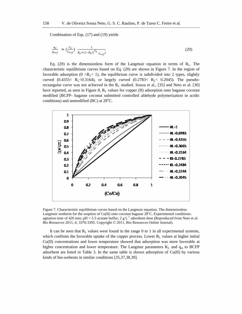
Eq. (20) is the dimensionless form of the Langmuir equation in terms of RL. The
characteristic equilibrium curves based on Eq. (20) are shown in Figure 7. In the region of
favorable adsorption (0 <RL< 1), the equilibrium curve is subdivided into 2 types, slightly
curved (0.4355< RL<0.3164), or largely curved (0.2783< RL< 0.2045). The pseudo-
rectangular curve was not achieved in the RL studied. Souza et al., [35] and Neto et al. [30]
have reported, as seen in Figure 8, RL values for copper (II) adsorption onto bagasse coconut
modified (BCFP- bagasse coconut submitted controlled aldehyde polymerization in acidic
conditions) and unmodified (BC) at 28oC.
Figure 7. Characteristic equilibrium curves based on the Langmuir equation. The dimensionless
Langmuir isotherm for the sorption of Cu(II) onto coconut bagasse 28oC. Experimental conditions:
agitation time of 420 min; pH = 5.5 acetate buffer; 2 g L-1
adsorbent dose (Reproduced from Neto et al.
Bio Resources 2011, 6, 3376-3395. Copyright © 2011, Bio Resources Online Journal).
It can be seen that RL values were found in the range 0 to 1 in all experimental systems,
which confirms the favorable uptake of the copper process. Lower RL values at higher initial
Cu(II) concentrations and lower temperature showed that adsorption was more favorable at
higher concentration and lower temperature. The Langmur parameters KL and qm to BCFP
adsorbent are listed in Table 3. In the same table is shown adsorption of Cu(II) by various
kinds of bio-sorbents in similar conditions [35,37,38,39].

Equilibrium and Kinetic Studies in Adsorption of Toxic Metal Ions ... 159
Figure 8. RL values for Cu (II) adsorption onto coconut bagasse (BC) and coconut bagasse submitted
controlled aldehyde polymerization in acidic medium (BCFP). Experimental conditions: agitation time
of 420 min; pH = 5.5 acetate buffer; 2 g L-1
adsorbent dose (Reproduced with permission from Souza,
T.J.N.; Sousa et al, In: 8thBrazilian Adsorption Congress, Foz do Iguaçu (Paraná), September 19-22,
Ed. Universidade Estadual de Londrina, 2010. Copyright © 2010, EBA).
Table 3. Langmuir parameters for adsorption of Cu(II) by various kinds of biosorbents
in similar conditions (Reproduced with permission from Neto et al. Bio Resources. 2011,
6, 3376-3395. Copyright©2011, Bio Resources Online Journal)
Sorbent Operational conditions Parameters
Reference pH T(
oC) qm(mg.g
-1) KL(L.mg
-1)
Coconut bagasse
Modified (BCFP) 5.5 28 125 1.11x10
-2 [35]
Caulerpalentillifera 5.0 - 5.57 0.076 [37]
Lignin tannin gel 5.5 20 22.87 0.4309 [38]
Rice husk
(tartaric acid odified 5.2 27 29.00 0.100 [39]
3.1.3. Temkin Isotherm
Temkin and Pyzhev [40] considered the effects of some indirect sorbate/adsorbate
interactions on adsorption isotherms and suggested that because of these interactions the heat
of adsorption of all the molecules in the layer would decrease linearly with coverage. The
Temkin isotherm has been generally applied in the following form:

V. de Oliveira Sousa Neto, G. S. C. Raulino, P. de Tarso C. Freire et al. 160
(21)
and can be linearized as:
(22)
where B = RT/b, b is the Temkin constant related to heat of sorption (J.mol-1
); A is the
Temkin isotherm constant (L.mg-1
), R the gas constant (8.314 J.mol-1
.K-1
) and T the absolute
temperature (K). Therefore, by plotting qe versus lnCe enables one to determine the constants
A and b using the Figure 9. The constants A and b are listed in Table 4 [41, 42, 43].
3.1.4. Dubinin–Radushkevich (D-R) Isotherm
Langmuir and Freundlich isotherms do not give any idea about the sorption mechanism
but the former describes sorption on a single type of sorption site. In this respect the D-R
isotherm is an analogue of Langmuir type but it is more general because it does not assume a
homogeneous surface or constant sorption potential.
The equilibrium data can be also applied to the D-R model [44, 45] to determine the type
of sorption (physical or chemical). The linear form of D-R isotherm is presented as the
following equation:
ln(qe) = ln(qm) - βε2 (23)
where qe is the amount of Cu(II) adsorbed onto the per unit dosage of BC
(mol.g-1
), qm is the theoretical monolayer sorption capacity (mol.g-1
), β is the constant of the
sorption energy (mol2J
-2), which is related to the average energy of sorption per mole of the
sorbate as it is transferred to the surface of the solid from infinite distance in the solution and,
is the Polanyi potential, which is described by equation (24) where T is the solution
temperature (K) and R is the gas constant.
RTln(1+ ) (24)
The value of mean sorption energy, E (kJ/mol), can be calculated from D-R parameter β,
which is obtained from Figure 10, as follows:
E= (25)
The value of mean sorption energy gives information about chemical and physical
sorption. The E value ranges from 1 kJ.mol-1
to 8 kJ.mol-1
for physical sorption and from 8
kJ.mol-1
to 16 kJ.mol-1
for chemical sorption [46]. Souzaet al., [35] found mean sorption
energy, E (kJ/mol) = 10.85 kJ.mol-1
indicating that the type of sorption of Cu(II) on coconut
bagasse submitted controlled aldehyde polymerization in acidic medium (BCFP) is a
chemical sorption process (Figure 10). In Table 5, the D-R parameters are shown.
)ln( ee ACb
RTq
)ln()ln( ee CBABq

Equilibrium and Kinetic Studies in Adsorption of Toxic Metal Ions ... 161
The estimated parameters of the several models (Langmur, Freundlich, Temkin, and
Dubinin-Raduskevich) are shown in Table 5. Figure 11 shows the isotherm models are in
good agreement with experimental data.
Table 4. Temkin parameters for adsorption of Cu(II) by various kinds of biosorbents in
similar conditions (Reproduced with permission from Neto et al. Bio Resources. 2011, 6,
3376-3395. Copyright©2011, Bio Resources Online Journal)
Sorbent
Conditions Parameters
Reference pH T(oC) A
(L mg-1
)
b
(J.Mol-1
)
R2
Coconut bagasse modified
BCFP 5.5 28 0.3071 137 0.934 [35]
Undariapinnatifida 4.0 - 0.617 144.1 0.982 [41]
Mimosa tannin gel 5.0 25 0.019 404 0.964 [42]
H3PO4-activated rubber wood
sawdust 6.0 30 0.140 3467 0.938 [43]
Figure 9. Temkin adsorption isotherm obtained by using the linear method for the Cu(II) sorption onto
coconut bagasse submitted controlled aldehyde polymerization in acidic medium. Experimental
conditions: agitation time of 420 min; pH = 5.5 acetate buffer; 2 g L-1
adsorbent dose (Reproduced with
permission from Souza, T.J.N.; Sousa et al, In: 8thBrazilian Adsorption Congress, Foz do Iguaçu
(Paraná), September 19-22, Ed. Universidade Estadual de Londrina, 2010. Copyright © 2010, EBA).

V. de Oliveira Sousa Neto, G. S. C. Raulino, P. de Tarso C. Freire et al. 162
Figure 10. D-R linear equation obtained by using the linear method for the sorption of Cu(II) onto
coconut bagasse submitted controlled aldehyde polymerization in acidic medium. Experimental
conditions: agitation time of 420 min; pH = 5.5 acetate buffer; 2 g L-1
adsorbent dose (Reproduced with
permission from Souza, T.J.N.; Sousa et al, In: 8thBrazilian Adsorption Congress, Foz do Iguaçu
(Paraná), September 19-22, Ed. Universidade Estadual de Londrina, 2010. Copyright © 2010, EBA).
Figure 11. Theoretical adsorption isotherms and experimental data for Cu (II) adsorption onto bagasse
coconut. Experimental conditions: agitation time: 420 min; pH = 5.5 acetate buffer; adsorbent dose: 2 g
L-1
at 28oC (Reproduced with permission from Neto et al. Bio Resources. 2011, 6, 3376-3395.
Copyright © 2011, Bio Resources Online Journal).
Equilibrium and Kinetic Studies in Adsorption of Toxic Metal Ions ... 163
Table 5. Langmuir, Freundlich, Temkin, and D-R isotherm model parameters and
correlation coefficients for Cu (II) adsorption onto coconut bagasse modified BCFP at
28oC (Reproduced with permission from Neto et al. Bio Resources. 2011, 6, 3376-3395.
Copyright©2011, Bio Resources Online Journal)
Isotherm parameters Parameter values
Langmuir
qm(mg g-1
) 115
KL(L mg-1
) 1.2x10⁻³
R2 0.978
Freundlich
N 2.70
KF(mg g-1
)(L mg-1
)1/n
10.22
R2 0.969
Temkim
A(L mg-1
) 0.307
B 18.27
bT(J mol-1
) 137
R2
0.934
Dubinin-Redushkevich
qDR(mg g-1
) 178.7
(Mol J-1
)2 4.24x10
-9
E (kJ Mol-1
) 10.85
R2 0.976
4. ADSORPTION KINETICS
Kinetic studies help in predicting the progress of adsorption, but the determination of the
adsorption mechanism is also important for design purposes. In a solid–liquid adsorption
process, the transfer of the adsorbate is controlled by either boundary layer diffusion (external
mass transfer) or intra-particle diffusion (mass transfer through the pores), or by both.
4.1. Applications of Kinetic–Batch System
In order to understand the Cd (II) adsorption kinetic by low cost adsorbent (coconut
bagasse treated with thiourea/ammonia solution) pseudo first-order (PFO), second-order
(PSO), and intra-particle diffusion models were applied to the experimental data obtained
from batch studies. Kinetics is the study of the rates of chemical processes to understand the
factors that influence the rates. The study of chemical kinetics includes careful monitoring of
the experimental conditions which influence the speed of a chemical reaction and hence, help
attain equilibrium in a reasonable length of time. For example, Figure 12 shows the effect of
contact time on Cd (II) adsorption, and at least 51% Cd uptake was achieved for a
concentration of 100 mgL-1
in a very short period of contact of 5 min. Overall, the uptake rate

V. de Oliveira Sousa Neto, G. S. C. Raulino, P. de Tarso C. Freire et al. 164
of Cd (II) was high during the first 30 min, and about 90% of the total metal uptake occurred
during this period. However, the system continued to equilibrate for 25 to 120 min with
respect to Cd (II). Such studies yield information about the possible mechanism of adsorption
and the different transition states on the way to the formation of the final adsorbate-adsorbent
complex and help develop appropriate mathematical models to describe the interactions.
Figure 12. The effect of contact time on Cd (II) adsorption onto coconut bagasse treated with
thiourea/ammonia solution. Experimental conditions: Cd (II) = 100 mg L-1
, pH = 5.5 acetate buffer,
adsorbent dose of 2 g L-1
(Reproduced with permission from Neto et al. Bio Resources. 2012, 7, 1504-
1524. Copyright © 2012, Bio Resources Online Journal).
The kinetic parameters are helpful for the prediction of the adsorption rate, which gives
important information for designing and modeling the processes. In this chapter the
adsorption kinetics data experiment are analyzed using the pseudo-first-order, pseudo-second-
order, and intra-particle diffusion models are shown in Figures 13 and 14.
4.1.1. Pseudo-First-Order Kinetic Model (PFO)
Lagergren [47] suggested a rate equation for the sorption of solutes from a liquid
solution. This pseudo first-order rate model can be expressed as:
, (26)
where k1 (min−1
) is the pseudo first order adsorption rate coefficient. The integrated form of
the Eq. (26) for the boundary conditions of t=0,qt=0 and t=t, qt=qt, is
, (27)

Equilibrium and Kinetic Studies in Adsorption of Toxic Metal Ions ... 165
where qe and qt are the values of the amount adsorbed per unit mass at equilibrium and at any
time t. The values of k1 can be obtained from the slope of the linear plot of ln(qe- qt) versus t.
It is necessary to know the value of qe for fitting the experimental data to the Eq. (27).
Determining qe accurately is a difficult task, because in many adsorbate–adsorbent
interactions, the chemisorption becomes very slow after an initial fast response and it is
difficult to ascertain whether equilibrium is reached or not.
In such cases, an approximation has to be made about qe introducing an element of
uncertainty in the calculations. It is possible that the amount adsorbed even after a long
interaction time (taken as equivalent to equilibrium) is still appreciably smaller than the actual
equilibrium amount [48]. The value of k1 depends on the initial concentration of the adsorbate
that varies from one system to another. It usually decreases with the increasing initial
adsorbate concentration in the bulk phase [24]. For many adsorption processes, the Lagergren
pseudo first order model is found suitable only for the initial 20 to 30 min of interaction and it
is not good for the whole range of contact time [49].
Figure 13. Pseudo first-order model for Cd (II) onto coconut bagasse treated with thiourea/ammonia
solution. Experimental conditions: Cd(II) = 100 mg L-1
, pH = 5.5 acetate buffer, adsorbent dose of 2 g
L-1
(Reproduced with permission from Neto et al. Bio Resources. 2012, 7, 1504-1524. Copyright ©
2012, Bio Resources Online Journal).
A straight line of ln(qe-qt) versus t would indicate good applicability of the first-order
kinetics model since the experimental data agrees with the model data (see Figures 13 and
15). If this test is not valid, then higher order kinetic models are to be tested with respect to
the experimental results. In a true first-order process ln(qe) should be equal to the intercept of
a plot of ln(qe- qt) against t. The use of this linearization is based on the assumption that qe is
greater than qt. Finally if the Lagergren equation does not fit well in the whole range of
interaction time [49] obviously the adsorption process is following a much more complex
mechanism than the one based on simple first order kinetics. The value of the sorption rate
constant (k1) for Cd (II) adsorption by CBT was determined from the plot of ln(qe-qt) against t
(Figure 13). Although the coefficient of determination was higher than 0.97, the experimental
qe (33.5 mg g-1
) value did not agree with the calculated one (qe,cal = 23.6 mg g-1
).

V. de Oliveira Sousa Neto, G. S. C. Raulino, P. de Tarso C. Freire et al. 166
Thus, the pseudo-first-order model was unable to describe the time-dependent Cd (II)
sorption by CBT, as shown in Figure 15.
4.1.2. Pseudo Second-Order Model (PSO)
Another model that has been used for the analysis of sorption kinetics is the pseudo
second-order model. This model, proposed by Ho and McKay [50] is based on the
assumption that the adsorption follows second-order chemisorption. The pseudo second-order
model can be expressed as:
(28)
Separation of the variables followed by integration and application of the boundary
conditions (qt=0 at t=0 and qt=qt at t=t) yields a linear expression of the form
(29)
In this equation qe is the adsorption capacity at the equilibrium, qt(mg.g-1
) is the
individual capacity in a given time, k2 is the pseudo-second-order rate constants, and t is the
time. In cases where the pseudo-second-order model is well suited to the data, a plot of ( )
versus t gives a straight line with a slope of ( ) and an intercept of ( ). Values of these
parameters were obtained from Figure 14.
Figure 14. Pseudo second-order model for Cd(II) onto coconut bagasse treated with thiourea/ammonia
solution. Experimental conditions: Cd(II) = 100 mg L-1
, pH = 5.5 acetate buffer, adsorbent dose of 2 g
L-1
(Reproduced with permission from Neto et al. Bio Resources. 2012, 7, 1504-1524. Copyright ©
2012, Bio Resources Online Journal).
As shown in Figure 15, results obtained by using the pseudo-second-order rate equation
showed that the calculated value agreed very well with the experimental data, as can be

Equilibrium and Kinetic Studies in Adsorption of Toxic Metal Ions ... 167
observed in Table 5. The results obtained using the pseudo first-order and the pseudo second-
order equations with the parameters values for kineticrates (k1,k2); adsorption capacity
(qe,calcalculated, qe,exp, experimental), correlation coefficient (R2) and average percentage error
(APE) are presented in Table 6.
Figure 15. Comparison of experimental and predicted kinetic models in Cd(II) adsorption process onto
coconut bagasse treated with thiourea/ammonia solution.. Experimental conditions: Cd(II) = 100 mg L-
1, pH = 5.5 acetate buffer, adsorbent dose of 2 g L
-1 (Reproduced with permission from Neto et al. Bio
Resources. 2012, 7, 1504-1524. Copyright © 2012, Bio Resources Online Journal).
Table 6. Results for the Cd(II) sorption onto coconut bagasse treated with
thiourea/ammonia obtained by the pseudo first-order and pseudo second-order rate
equations using the linear method (Reproduced with permission from Neto et al. Bio
Resources. 2012, 6, 1504-1524. Copyright©2012, Bio Resources Online Journal)
qe, exp
(mg.g-1)
Pseudo first-order Pseudo second-order
qe,cal
(mg g-1)
k1
(min-1)
R2 APE
(%)
qe,cal
(mg g-1)
k2
(g mg-1min-1)
R2 APE
(%)
33.5 23.6 5.91x10⁻³ 0.971 5.2 35.5 4.45x10⁻³ 0.997 0.23
Results of related studies also have indicated the pseudo second-order kinetic model as
being suitable for Cd (II) sorption by non-treated biomasses [51-56].
4.1.3. Intra-Particle Diffusion Model
An intra-particle diffusion process tends to control the adsorption rate in systems
characterized by high concentrations of adsorbate, good mixing, and big particle size of
adsorbent [57]. Also, it has been noticed in some studies that boundary layer diffusion is
dominant during the initial adsorbate uptake, and then gradually the adsorption rate becomes
controlled by intra-particle diffusion after the adsorbent’s external surface has become loaded
with the adsorbate. In order to gain insight into the mechanisms and rate-controlling steps
affecting the kinetics of adsorption, it is possible to use different models. In this chapter we

V. de Oliveira Sousa Neto, G. S. C. Raulino, P. de Tarso C. Freire et al. 168
decided to discuss two of the most common diffusion models: Weber’s intra-particle diffusion
model [58] and Boyd’s diffusion model [59, 60].
4.1.4. Weber’s Intra-Particle Diffusion Model
Weber’s pore-diffusion model is commonly used in adsorption studies. It is defined by
the equation:
(30)
where C is the intercept and kid is the intra-particle diffusion rate constant (mg/g min 1/2
),
which can be evaluated from the slope of the linear plot of qt versus t1/2
. The values of C
provide information about the thickness of the boundary layer. In general, the larger the
intercept, the greater the boundary layer effect [61].
If intra-particle diffusion is controlling, then qt versus t1/2
will be linear, and if the plot
passes through the origin, then the rate limiting process is due only to intra-particle diffusion.
Otherwise, some other mechanism along with intra-particle diffusion must also be involved.
Pore-diffusion plots often show several linear segments. It has been proposed that these linear
segments represent pore-diffusion in pores of progressively smaller sizes [50].
Eventually, equilibrium is reached, and adsorption (qe) stops changing with time, and a
final horizontal line is established at qe. When points in a group are identified as belonging to
a linear segment, linear regression can then be applied to these points, and the corresponding
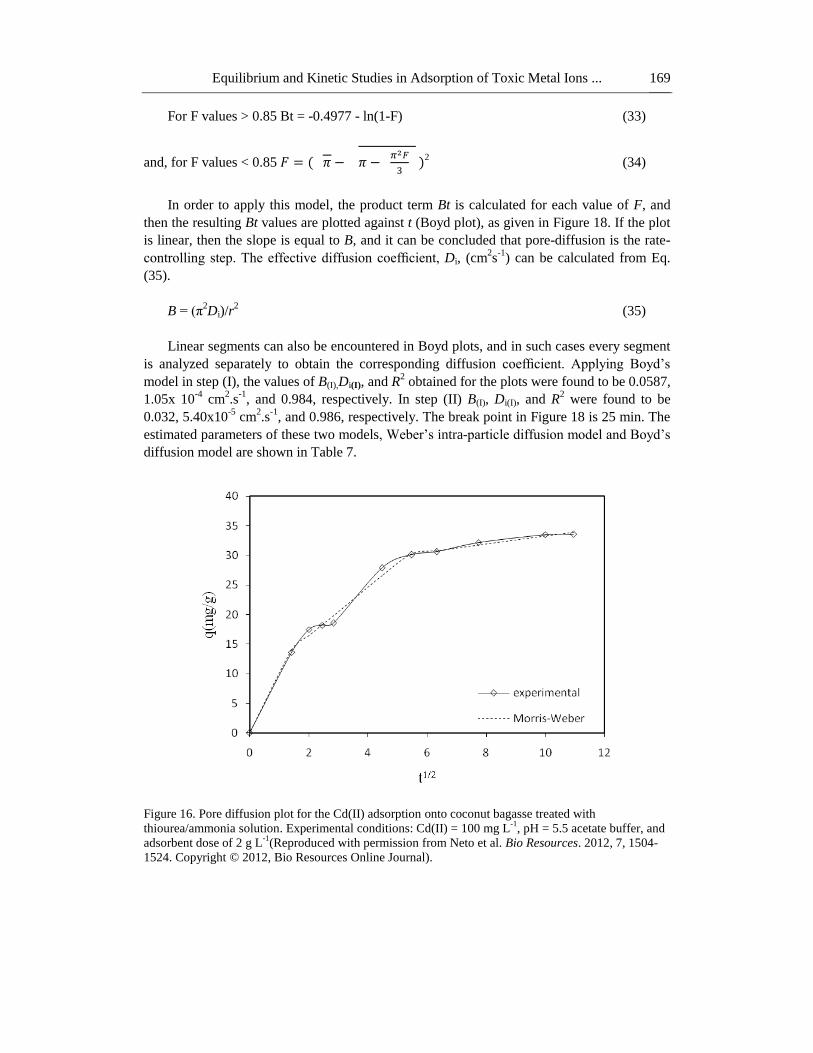
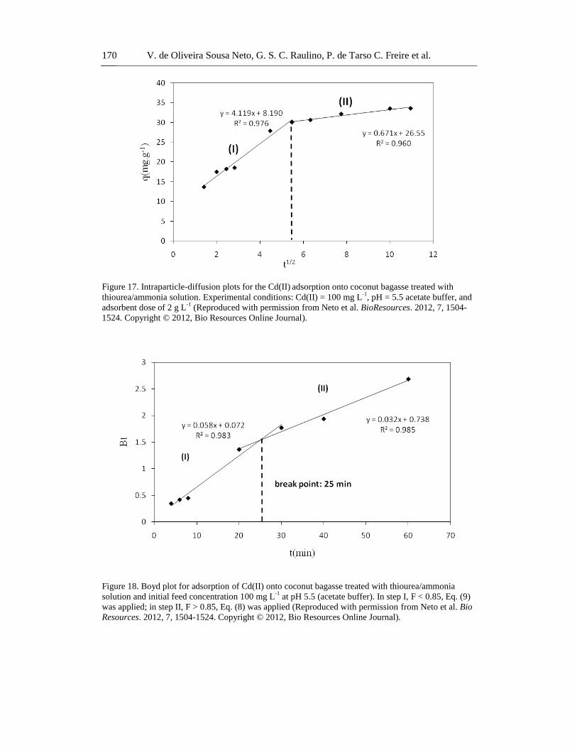
kid is estimated. Neto et al. [62] studied the mechanism involved on Cd(II) adsorption onto
CBT adsorbent. The Cd(II) adsorption data were plotted according to Eq. 30, as shown in
Figure 16. As seen in Figure17, the points were not linear over the whole time range,
implying that more than one process affected the adsorption, and this deviation might be due
to the difference in the mass transfer rate of the initial and final stage of adsorption. This
indicates that diffusion into one class of pores was not the only rate-limiting mechanism in
the adsorption process. Applying Weber’s model in the step (I) the values of kid(I), C(I), and R2
obtained for the plots were 4.12 mg g-1
min-1/2
, 8.19 mg g-1
, and 0.976, respectively. In the step
(II) kid(II), C(II), and R2 were 0.672 mg g
-1min
-1/2, 26.55 mg g
-1, and 0.961, respectively. The
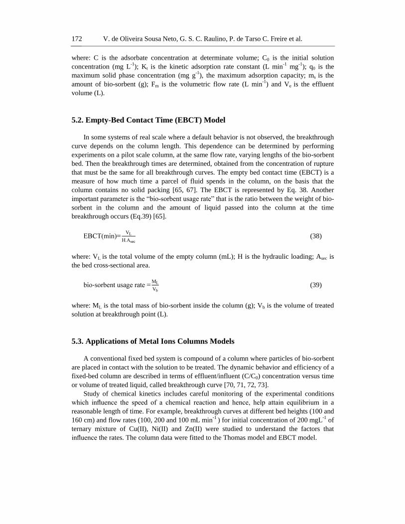
break point in Figure 17 is 28 min. To determine whether the adsorption process occurs via
external diffusion or intraparticle mechanism, the kinetic data were investigated by the model
of Boyd et al. [59, 60]. If diffusion inside the pores is the rate-limiting step, then the results
can be expressed as,
(31)
where B is a constant, and F is the fractional attainment of equilibrium at different times t
given by Eq. (32),
F = qt/qe (32)
where qt and qe are the Cd(II) uptakes (mg/g) in equilibrium, at a time t.
The term Bt is calculated by the following equations, due to Reichenberg [63]:
Ctkq idt 2/1
Equilibrium and Kinetic Studies in Adsorption of Toxic Metal Ions ... 169
For F values > 0.85 Bt = -0.4977 - ln(1-F) (33)
and, for F values < 0.85 2 (34)
In order to apply this model, the product term Bt is calculated for each value of F, and
then the resulting Bt values are plotted against t (Boyd plot), as given in Figure 18. If the plot
is linear, then the slope is equal to B, and it can be concluded that pore-diffusion is the rate-
controlling step. The effective diffusion coefficient, Di, (cm2s
-1) can be calculated from Eq.
(35).
B = (π2Di)/r
2 (35)
Linear segments can also be encountered in Boyd plots, and in such cases every segment
is analyzed separately to obtain the corresponding diffusion coefficient. Applying Boyd’s
model in step (I), the values of B(I),Di(I), and R2 obtained for the plots were found to be 0.0587,
1.05x 10⁻⁴
cm2.s
-1, and 0.984, respectively. In step (II) B(I), Di(I), and R
2 were found to be
0.032, 5.40x10⁻⁵
cm2.s
-1, and 0.986, respectively. The break point in Figure 18 is 25 min. The
estimated parameters of these two models, Weber’s intra-particle diffusion model and Boyd’s
diffusion model are shown in Table 7.
Figure 16. Pore diffusion plot for the Cd(II) adsorption onto coconut bagasse treated with
thiourea/ammonia solution. Experimental conditions: Cd(II) = 100 mg L-1
, pH = 5.5 acetate buffer, and
adsorbent dose of 2 g L-1
(Reproduced with permission from Neto et al. Bio Resources. 2012, 7, 1504-
1524. Copyright © 2012, Bio Resources Online Journal).
V. de Oliveira Sousa Neto, G. S. C. Raulino, P. de Tarso C. Freire et al. 170
Figure 17. Intraparticle-diffusion plots for the Cd(II) adsorption onto coconut bagasse treated with
thiourea/ammonia solution. Experimental conditions: Cd(II) = 100 mg L-1
, pH = 5.5 acetate buffer, and
adsorbent dose of 2 g L-1
(Reproduced with permission from Neto et al. BioResources. 2012, 7, 1504-
1524. Copyright © 2012, Bio Resources Online Journal).
Figure 18. Boyd plot for adsorption of Cd(II) onto coconut bagasse treated with thiourea/ammonia
solution and initial feed concentration 100 mg L-1
at pH 5.5 (acetate buffer). In step I, F < 0.85, Eq. (9)
was applied; in step II, F > 0.85, Eq. (8) was applied (Reproduced with permission from Neto et al. Bio
Resources. 2012, 7, 1504-1524. Copyright © 2012, Bio Resources Online Journal).

Equilibrium and Kinetic Studies in Adsorption of Toxic Metal Ions ... 171
Table 7. Results for the Cd(II) sorption onto coconut bagasse treated with
thiourea/ammonia obtained by Weber’s pore-diffusion model and Boyd’s diffusion
model by using the linear method (Reproduced with permission from Neto et al. Bio
Resources. 2012, 6, 1504-1524. Copyright©2012, Bio Resources Online Journal)
Webers’s pore-diffusion model
I II
Kid(I)
(mg.g-1
min-1/2
)
C1
mg.g-1
R2 Kid(II)
(mg.g-1
min-1/2
)
C2
mgg-1
R
2
4.12 8.19 0.976 0.672 26.55 0.961
Boyd’s diffusion model
I II
B Di(I)
(cm2.s
-1)
R2
B Di(II)
(cm2.s
-1)
R2
0.0587 1.05x 10⁻⁴
0.9838 0.032 5.40x10⁻⁵
0.9858
5. COLUMN ADSORPTION MODELS
The performance of the column can be predicted by various mathematical models. In this
chapter the Thomas model [64] and the Empty-bed Contact Time (EBCT) [65] model have
been applied to the predicted breakthrough curve and to calculate the column kinetics
constant, maximum capacity adsorption of fixed bed adsorption.
5.1. Thomas Model
This model assumes a behavior of continuous flow and uses the Langmuir isotherm for
equilibrium and reversible second-order kinetics reaction. It is applicable for favorable and
unfavorable adsorption conditions [66].
Traditionally, this model is used to determine the maximum adsorption capacity of bio-
sorbent in continuous systems considering external and internal as the limiting steps. The
Thomas model is expressed by Eq. 36. [67, 68, 69, 70].
(36)
The adsorption capacity of the bed q0 and the coefficient Kt may be obtained from the
intercept and slope, respectively, of a curve obtained by plotting ln (C/C0 - 1) as a function of
t or Ve from the breakthrough point Cb until exhaustion point Cx, but these constants can be
obtained using non-linear regression analysis.
The Thomas model can be linearized as
(37)
V. de Oliveira Sousa Neto, G. S. C. Raulino, P. de Tarso C. Freire et al. 172
where: C is the adsorbate concentration at determinate volume; C0 is the initial solution
concentration (mg L-1
); Kt is the kinetic adsorption rate constant (L min-1
mg-1
); q0 is the
maximum solid phase concentration (mg g-1
), the maximum adsorption capacity; ms is the
amount of bio-sorbent (g); Fm is the volumetric flow rate (L min-1
) and Ve is the effluent
volume (L).
5.2. Empty-Bed Contact Time (EBCT) Model
In some systems of real scale where a default behavior is not observed, the breakthrough
curve depends on the column length. This dependence can be determined by performing
experiments on a pilot scale column, at the same flow rate, varying lengths of the bio-sorbent
bed. Then the breakthrough times are determined, obtained from the concentration of rupture
that must be the same for all breakthrough curves. The empty bed contact time (EBCT) is a
measure of how much time a parcel of fluid spends in the column, on the basis that the
column contains no solid packing [65, 67]. The EBCT is represented by Eq. 38. Another
important parameter is the “bio-sorbent usage rate” that is the ratio between the weight of bio-
sorbent in the column and the amount of liquid passed into the column at the time
breakthrough occurs (Eq.39) [65].
(38)
where: VL is the total volume of the empty column (mL); H is the hydraulic loading; Asec is
the bed cross-sectional area.
- (39)
where: ML is the total mass of bio-sorbent inside the column (g); Vb is the volume of treated
solution at breakthrough point (L).
5.3. Applications of Metal Ions Columns Models
A conventional fixed bed system is compound of a column where particles of bio-sorbent
are placed in contact with the solution to be treated. The dynamic behavior and efficiency of a
fixed-bed column are described in terms of effluent/influent (C/C0) concentration versus time
or volume of treated liquid, called breakthrough curve [70, 71, 72, 73].
Study of chemical kinetics includes careful monitoring of the experimental conditions
which influence the speed of a chemical reaction and hence, help attain equilibrium in a
reasonable length of time. For example, breakthrough curves at different bed heights (100 and
160 cm) and flow rates (100, 200 and 100 mL min-1
) for initial concentration of 200 mgL-1
of
ternary mixture of Cu(II), Ni(II) and Zn(II) were studied to understand the factors that
influence the rates. The column data were fitted to the Thomas model and EBCT model.

Equilibrium and Kinetic Studies in Adsorption of Toxic Metal Ions ... 173
The characterization of bio-sorbent bed (green coconut shell powder) used for this study
is given in Table 8.
Table 8. Physical parameters of biosorbent (green coconut shell powder)
and column system
Property Green coconut shell
Column diameter (dL) (cm) 6.2 6.2 6.2
Bed height (cm) 100 100 160
Total area of the column (cm2) 2007.15 2007.15 3175.23
Volume of the empty column (VL) (cm3) 3017.54 3017.54 4828.06
Mass of biosorbent in the column (g) 402 480 600
Apparent density (ρap) (g cm-3
) 0.188 0.188 0.188
Packing density (ρE) (g cm-3
) 0.133 0.159 0.124
Particle volume (Vap) (cm3) 2138.29 2553.2 3191.48
Porosity of the bed (ε) 0.292 0.154 0.338
5.3.1. Breakthrough Curves
5.3.1.1. Flow Rate Effect
The experimental and theoretical breakthrough curves for three flow rates studied are
shown in Figure 19. Adsorption capacities of bio-sorbent were determined by equation 36.
According the Vb and Vx values in Table 9, it can be seen that as the flow rate increases,
the rupture volume of metal ions studied decreases, and there is a decrease in the adsorption
capacity of the adsorbent for each metal. The increase in flow rates implies the reduction of
the hydraulic retention time (HRT) of metal ions inside the column.
According to Cooney [65], HRT is a typical parameter of design and operation for
columns and the usual residence times range from 15 to 30 minutes. Residence times larger
than these can lead to a decrease in the removal of the contaminant, while shorter times do not
allow an effective contact interaction to occur between the sorbent and sorbate [65,74].
The HRT is given by the ratio between the reactor volume (in this case, column) and flow
rate. Table 9 shows that HRT decreased from 30 to 10 minutes when the flow rate increased
from 100 to 300 mL min-1
. Thus, analyzing the breakthrough curves, the adsorption capacity
and the HRT, the flow rate of 200 mL min-1
can be chosen for the following studies.
The Thomas model was applied to the experimental data (continuous line in Figure 19).
Except for copper, the Thomas model well represented the flow rate data. A linear plot of
ln[(C0/C) - 1] versus Ve(L) to data located at 0.05 < C/C0 < 0.90 enabled a previous
determination of the Thomas rate constant, Kt, and adsorption capacity of the bed, q0,
according to equation 37. Nonlinear regression analysis was performed using Eq. (36).

Table 9. Breakthrough volumes (Vb), exhaustion volumes (Vx) and adsorption capacity (when C/C0 = 0.5) obtained for each metal
on studied flow rates
Metal ion Flow rate (mL min-1
) / HRT (min)
100 / 30 200 / 15 300 / 10
Vb (L) Vx (L) q0 (mg g-1
) Vb (L) Vx (L) q0 (mg g-1
) Vb (L) Vx (L) q0 (mg g-1
)
Cu (II) 30.7 55.0* 14.8 25.3 61.0* 13.83 18.75 78.0* 10.95
Ni (II) 9.5 16.0 4.17 8.6 14.6 5.43 7.0 11.1 2.98
Zn (II)
9.9 16.9 4.67 9.0 13.9 4.53 7.0 12.3 3.29
* Estimated values.
Table 10. Parameters by linear (L) nonlinear regression (NL) analysis with Thomas model for metal ions Cu (II),
Ni (II) and Zn (II) for three flow rates studied
Metal ion Flow rate (mL min-1
) Kt (mL min-1
mg-1
) q0 (mg g-1
) SSE
L NL Theoretical Experimental L NL
L NL
Cu (II) 100 0.102 0.113 15.40 15.36 14.80 0.061 1.36 E-29
200 0.091 0.270 16.34 14.90 13.83 9.142 2.31 E-07
300
0.292 0.299 12.13 11.43 10.95 0.428 1.69 E-29
Ni (II) 100 0.462 0.460 4.43 4.42 4.17 1.53 E-3 3.77 E-32
200 1.008 1.141 5.65 5.36 5.43 0.357 4.44 E-31
300
3.478 3.464 3.16 2.90 2.98 1.42 2.99 E-14

Table 10. (Continued)
Metal ion Flow rate (mL min-1
) Kt (mL min-1
mg-1
) q0 (mg g-1
) SSE
L NL Theoretical Experimental L NL
L NL
Zn (II) 100 0.412 0.410 4.90 4.89 4.67 3.35 E-4 1.17 E-28
200 1,203 1.119 4.67 4.67 4.53 6.737 4.07 E-31
300
2.716 1.991 3.73 3.27 3.29 1.059 6.84 E-13

V. de Oliveira Sousa Neto, G. S. C. Raulino, P. de Tarso C. Freire et al. 176
The sum of the squares of the errors (SSE) Eq. (37) was examined for every experimental
data set and the parameters of Kt and q0 were determined for the lowest error values in each
case, by adjusting and optimizing the functions themselves using the solver add-in for
Microsoft Excel®. The values of Kt and q0 obtained for the lowest error values are shown in
Table 10. The sum of the squares of the errors (SSE) is given in Eq. (40) [75]:
(40)
where qe is the adsorption capacity determinate from the column experiment i; qcal is the
estimated adsorption capacity and P is the number of parameters in the regression model. The
smaller function value indicates the best curve fitting. In general, the theoretical and
experimental maximum adsorption capacities were closed. The increase in the flow rate
resulted in an increase of Thomas rate constant and a decrease in maximum adsorption
capacities for the metals studied.
In Figure 19 we see that for copper, the model does not fit well with experimental data at
the three flow rates studied. For nickel and zinc, there was a better fit until C/C0 = 1, from
which there was desorption of metal ions, and distance between experimental data and
theoretical model. The non-linear (NL) regression analyses represented the data better than
linear (L) regression analyses.
In the Table 10 we can see that the errors for NL were lower than L, showing a better fit.
The increase in the flow rate (100 to 300 mL min-1
) resulted in the increase of Thomas
rate constant and a decrease in maximum adsorption capacities for all metals ions studied for
an initial metal concentration of 200 mg L-1
.
The Thomas rate constants for the metal ion system investigated follow the order.
According to Table 10, by increasing the flow rate at 3 times the Thomas rate constant (Kt)
increases 3, 8 and 10 times for Cu(II), Ni (II) and Zn (II) respectively, due the metal ions rate
transfer from the solution to the bed fixed column because of the driving force for adsorption
[66]. However, in contrast with increasing flow rate (100 to 300 mL min-1
) the adsorption
capacity values decrease, (qo ,mg g-1
) but not all the metal ions will have enough time to
penetrate from solution to the coconut shell pores and bind to the functional group, resulting
in a lower removal of Cu(II), Ni(II) and Zn(II).
A
Figure 19. (Continued)

Equilibrium and Kinetic Studies in Adsorption of Toxic Metal Ions ... 177
B
C
Figure 19. Comparison of experimental and theoretical breakthrough curves of metal ions at varied flow
rates of: (A) 100 mL min-1
, (B) 200 mL min-1
and (C) 300 mL min-1
.
This can be due to the driving force for adsorption caused by the higher ion
concentration. A similar trend was observed by Shahbazi et al.[76] on the Pb(II), Cu(II) and
Cu(II) removal by functionalized mesoporous silica. On the other hand, Revathi et al. [66]
observed that as the flow rate increased, the adsorption capacity and kinetic rate constant of
Thomas increased with higher zinc concentration on exchange resin of Amberlite IR 120. In
Figure 19 we can see that for copper, the model does not fit well with experimental data at the
three flow rates studied. For nickel and zinc, there was a better fit until C/C0 = 1, from which
there was desorption of metal ions, and distance between experimental data and theoretical
model. Having the values of Kt and q0 of each metal, it is possible to obtain the total mass of
bio-sorbent required to treat wastewater in a column, under the same conditions, requiring
only to know the feed concentration of each metal, the daily flow rate and volume of solution
to be treated.

V. de Oliveira Sousa Neto, G. S. C. Raulino, P. de Tarso C. Freire et al. 178
5.3.2. Bed Height
From the breakthrough curves (shown in Figure 20) obtained by the study of two bed
heights 100 cm (Figure 20a) and 160 cm (Figure 20b) filled with 480 and 600 g of bio-
sorbent, respectively. Multi-component synthetic solutions were percolated through the
column at a flow rate of 200 mL min-1
.
Height and the adsorption capacities, and EBCT model are given in Tables 11 and 12,
and can be noted (Table 11) that the breakthrough volume of each metal increased with the
increase of bed height. Several works report that the greater the bed height is, the greater the
service time of the column, since the surface area of bio-sorbent is increased as the amount of
active sites available for metal-bio-sorbent interaction. In addition, the bio-sorbent capacity of
the material also increases with increasing bed height [65, 77, 78]. The maximum HRT, cited
by Cooney [65], of 35 minutes, is not exceeded when column increases from 100 to 160cm.
Table 11. Breakthrough volumes (Vb), exhaustion volumes (Vx) and adsorption capacity
(when C/C0 = 0.5) obtained for each metal on studied bed heights
Metal Ion
Bed Heights (cm) / HRT (min.)
100 / 15 160 / 24
Vb (L) Vx (L) Q (mg.g-1
) Vb (L) Vx (L) Q (mgg-1
)
Cu (II) 25.3 61.0* 13.83 44.0 68.0* 16.84
Ni (II) 8.60 14.6 5.43 11.3 28.0 6.56
Zn (II)
8.90 13.9 4.53 13.0 17.8 4.96
* Estimated values.
Table 12. EBCT and biosorbent usage rate at different bed height
Metal ion Bed heights
(cm)
EBCT
(min)
Biosorbent mass
(g)
Breakthrough
volume (L)
BUR
(g L-1
)
Cu (II) 100 15 480 25.3 18.97
160 24 600 44.0 13.63
Ni (II) 100 15 480 8.6 55.8
160 24 600 11.3 53.1
Zn (II) 100 15 480 8.9 53.9
160 24 600 13.0 46.15
Applying EBCT model and bio-sorbent usage rate (Equations 38 and 39), for
experimental data in Table 12 can be observed that increasing the bed height, the HRT and
breakthrough volume (Vb) increases. Consequently, the amount of bio-sorbent used per liter
of effluent solution processed decreases. [65, 77, 78] It was reported that the greater the
EBCT, the lower the bio-sorbent amount required to treat the same volume of solution at the
same concentration. The bio-sorbent usage rate (BUR) is lower for copper due to the effect of
competition between metal ions in solution by bio-sorbent sites.

Equilibrium and Kinetic Studies in Adsorption of Toxic Metal Ions ... 179
A
B
Figure 20. Breakthrough curves of metal ions to bed heights: (a) 100 cm and, (b) 160 cm.
CONCLUSION
In this study the results showed that the coconut bagasse modified with
thiourea/amonium and coconut bagasse are promising adsorbents for the removal of Cd(II)
and Cu(II) from aqueous solutions. Adsorption equilibrium data showed good fits to the

V. de Oliveira Sousa Neto, G. S. C. Raulino, P. de Tarso C. Freire et al. 180
Langmuir, and Temkin isotherm models, as well as adsorption kinetic data following a
second order kinetic model, but intra-particle diffusion was not the only rate-controlling step.
The study of fixed-bed column adsorption for the removal of Cu(II), Ni(II) and Zn(II)
showed that greater the bed height, the greater is the bio-sorbent adsorption capacity and a
smaller amount of bio-sorbent material is required per liter of solution to be treated.
Since that investigation new adsorbents are continuously being developed, introducing
new applications for adsorption technology, and coconut bagasse can be exploited as a bio-
adsorbent for metal removal from aqueous solutions. Additionally, the use of modeling for
adsorption equilibrium and adsorption kinetic is important in order to select the optimum
condition for full-scale batch and column processes for metal removal from industrial
effluent.
ACKNOWLEDGMENTS
The authors thank to Brazilian Council of Research and Development (CNPq, Process
No. 306114/2008-9); and Ceará State Foundation for the Scientific Support and technological
development (FUNCAP), and the Federal University of Ceará.
REFERENCES
[1] Othman, Z.A.; Ali, R.; Naushad, M. Chemical Eng. J. 2012, 184, 238-247.
[2] Semerjian, L.; Ayoub, G.M. Adv. Environ. Res.2003, 7, 389-403.
[3] Tunay, O.; Water Sci. Technol. 2003, 48, 43-52.
[4] Wang, L. K.; Vaccari, D. A.; Li, Y.; Shammas, N. K. in Physicochemical Treatment
Processes; Wang, L. K.; Hung, Y. T.; Shammas, N. K. (Eds.); Humana Press: New
Jersey (NJ), 2004; Vol. 3, pp 141-198.
[5] Chen, G. H., Sep. Purif. Technol. 2004, 38, 11-41.
[6] Sapari, N.; Idris, A.; Hisham, N. Desalination 1996, 106, 419-422.
[7] Volesky, B.Hydrometallurgy, 2001, 59, 203-216.
[8] Sud, D.; Mahajan, G.; Kaur, M. P. Bioresour. Technol, 2008, 99, 6017 - 6027.
[9] Sparks, D. L. Environmental Soil Chemistry; 2th Ed..; Academic Press: San Diego, CA.
2003, Vol. 1, pp 1-352.
[10] Weber, W.J.; Smith, E.H. Environ. Sci. Technol. 1988, 21, 1040-1050.
[11] Stumm, W. Chemistry of the solid-water interface: processes at the mineral-water and
particle water interface in natural systems, Chapter 4, Wiley-Interscience: New York,
NY, 1992, Vol 1, pp 87-145.
[12] Sawyer, C. N.; McCarty, P. L.; Parklin, G. F. Chemistry for environmental engineering.
4th ed. McGraw-Hill Book Company: New York, NY. 1994, Vol 1, 658p.
[13] Do, D. D., Adsorption Analysis: Equilibria and Kinetics; Chemical Engineer Series;
Imperial College Press: Covent Garden, London, 1998, Vol. 2, pp. 11-18.
[14] Ruthven, D. M., Principles of Adsorption and Adsorption Processes, Wiley-
Interscience: New York, NY, 1984, Vol 1, pp. 30-34.
[15] Yang, R. T. Gas Separation by Adsorption Process, Chemical Engineer Series;
Imperial College Press: London, 1998, Vol 1, pp. 28-35.

Equilibrium and Kinetic Studies in Adsorption of Toxic Metal Ions ... 181
[16] Metcalf and Eddy Wastewater Engineering: Treatment and Reuse; McGraw-Hill
Science/Engineering/Math: New York, NY, 2003; Vol. 1, pp.478-483.
[17] Vegliò, F.; Beolchini, F. Hydrometallurgy 1997, 44, 301-316.
[18] Kolthoff, I. M.; Sandell, E. B.; Meehan, E. J.; Bruckenstein, S. Quantitative Chemical
Analysis, 4th
Ed.; McMillan: New York, NY, 1969; 1146 p.
[19] Harris, D. C. Quantitative Chemical Analysis, 6th Ed.; W. H. Freeman: New York, NY,
2002; 809 p.
[20] Foo, K. Y.; Hameed, B. H. Chem. Eng. J. 2010, 156, 2-10.
[21] Martín-Lara, M. A.; Pagnanelli, F.; Mainelli, S.; Calero, M.; Toro, L. J. Hazardous
Mat. 2008, 156, 448-457.
[22] Febrianto, J.; Kosasih, A. N.; Sunarso, J.; Ju, Y-H.; Indraswati, N.; Ismadji, S. J.
Hazardous Mat. 2009, 162, 616-645.
[23] Malek, A.; Farooq, S. AIChE J. 1996, 42, 3191-3201.
[24] Allen, S. J.; Gan, Q.; Matthews, R.; Johnson, P. A. J. Colloid Interface Sci. 2005, 286,
101-109.
[25] Dubinin, M.M. Chem. Rev. 1960, 60, 235-266.
[26] Myers, A.L. Prausnitz, J.M. AIChE J. 1965, 11, 121-129.
[27] Limousin, G.; Gaudet, J.P.; Charlet, L.; Szenknect, S.; Barthes, V.; Krimissa, M.; Appl.
Geochem. 2007, 22, 249-275.
[28] Allen, S.J.; Mckay, G.; Porter, J.F.; J. Colloid Interface Sci. 2004, 280, 322-333.
[29] Freundlich, H. M. F., Z. Phys. Chem. 1906, 57, 385-470.
[30] Neto, V. O. S.; Oliveira A. G.; Teixeira, R. N. P.; Silva, M. A. A.; Freire, P. T. C.;
Keukeleire, D. D.; Nascimento, R. F. BioResources 2011, 6, 3376-3395.
[31] Vijayaraghavan, K.; Palanivelu, K.; Velan, M. Bioresour. Technol. 2006, 97, 1411-
1419.
[32] Cay, S.; Uyanik, A.; Ozasik, A. Sep. Sci. Technol. 2004, 38, 273-280.
[33] Djeribi, R.; Hamdaoui, O. Desalination 2008, 225, 95-112.
[34] Amarasinghe, B. M. W. P. K.; Williams, R. A. Chem. Eng. J. 2007, 132, 299-309.
[35] Souza, T.J.N.; Sousa, F. W.; Oliveira, A. G.; Moreira, S. A.; Nascimento, R.F.; Neto,
V. O. S. In: 8th
Brazilian Adsorption Congress, Foz do Iguaçu (Paraná), September 19-
22, Ed. Universidade Estadual de Londrina, 2010.
[36] Weber, T.W.; Chakarvorti, R.K. AIChE Journal, 1974, 20, 228-237.
[37] Pasavant, P.; Apiratikul, R.; Sungkhum, V.; Suthiparinyanont, P.; Wattanachira, S.
Marhaba, T. F. Bioresour. Technol. 2006, 97, 2321-2329.
[38] Guo, X. Y.; Zhang, A. Z.; Shan, X. Q., J. Hazard. Mat. 2008, 151, 134-142.
[39] Wong, K. K.; Lee, C. K.; Low, K. S.; Haron, M. J. Chemosphere 2003, 50, 23-28.
[40] Temkin, M.; Pyzhev, V. Acta Physiochim. USSR 1940, 12, 217-222.
[41] Chen, Z.; Ma, W.; Han, M.; J. Hazard. Mat. 2008. 155, 327-333.
[42] Şengil, A., and Özacar, M., J. Hazard. Mater. 2008 157, 277-285.
[43] Kalavathya, M. H.; Rajgopala, S. L.; Miranda, R. J. Colloid Interface Sci. 2005, 292,
354-362.
[44] Dubinin, MM.; Zaverina, E.D.; Radushkevich, L.V.; Zh. Fiz. Khim. 1947, 21, 1351-
1362.
[45] Saltalı, K.; Sarı, A.; Aydın, M. J. Hazard. Mat. 2007, 141, 258-263.
[46] Sarı, A.; Tuzen, M.; Cıtak, D.; Soylak, M. J. Hazard. Mat. 2007, 148, 387-394.

V. de Oliveira Sousa Neto, G. S. C. Raulino, P. de Tarso C. Freire et al. 182
[47] Lagergren, S.; Zur, B. K. S.; Veternskapsakad Handlingar 1898, 24,
1-39.
[48] Ungarish, M.; Aharoni, C. J ChemSoc Faraday Trans.1981, 77, 975-985.
[49] McKay, G.; Ho, Y.S.; Ng, J.C.Y. Sep Purif Methods 1999, 28, 87-125.
[50] Ho, Y. S.; McKay, G. Can. J. Chem. Eng. 1998, 76, 822-827.
[51] Jnr, M. H; Spiff, A. I. Electron. J. Biotechnol 2005, 8, 162-169.
[52] Pino, G. H.; Mesquita, L. M. S.; Torem, M. L.; Pinto, G. A. S. Miner. Eng. 2006, 19,
380-387.
[53] Vilar,V. J. P.; Botelho, C. M. S.; Boaventura, R. A. R., Water Res. 2006, 40, 291-302.
[54] Wang, X.; Xia, S.; Chen, L.; Zhao, J.; Chovelon, J.; Jaffrezic-Renault, N., J. Environ.
Sci. 2006, 18, 840-844.
[55] Mata, Y. N.; Blazquez, M. L.; Ballester, A.; Gonzalez, F.; Munoz, J. A. J. Hazard. Mat.
2008, 158, 316-323.
[56] Sarıa, A.; Tuzen, M. J. Hazard. Mat. 2009, 164, 1004-1011.
[57] Mohan, D.; Singh, K. P. Water Res. 2002, 36, 2304–2318.
[58] Weber Jr.; W. J.; Morris, J. C. J. Sanit. Eng. Div. Proceed. Am. Soc. Civil Eng. 1963,
89, 31-39.
[59] Boyd, G. E.; Schubert, J.; Adamson, A.W. J. Am. Chem. Soc. 1947. 69, 2818-2829.
[60] Boyd, G. E.; Adamson, A. W.; Myers Jr.; L. S. J. Am. Chem. Soc. 1947, 69, 2836-2848.
[61] Kavitha, D.; Namasivayam, C. Bioresour. Technol. 2007, 98, 14-21.
[62] Neto, V. O. S.; Carvalho, T. V.; Gomes, C. L.; Barros, F. C.; Araújo-Silva, M. A.;
Freire, P. T. C.; Nascimento, R. F. BioResources 2012, 7, 1504-1524.
[63] Reichenberg, D. J. Am. Chem. Soc. 1953, 75, 589-598.
[64] Thomas, H. C. J. Am. Chem. Soc.1953, 78, 243-249.
[65] Cooney, D. O. Adsorption Design for Wastewater Treatment. CRC press LLC: Boca
Raton, Florida, 1999; Vol 1, pp 1-180.
[66] Revathi, M.; Saravanan, M.; Chiya, A. B.; Velan, M. Clean-Soil, Air. 2012, 40, 66-79.
[67] Srivastava, V. C.; Prasad, B.; Mishra, I. M.; mall, I. D.; Swamy, M. M.Ind. Eng. Chem.
Res. 2008, 47, 1603-1613.
[68] Yan, G.; Viraraghavan, T. Bioresour. Technol. 2001, 78, 243-249.
[69] Vijayaraghavan, K.; Thilakavathi, M.; Palanivelu, K.; Velan, M. Environ. Technol.
2005, 26, 267-276.
[70] Aksu, Z.; Gönen, F.Sep. Sci. Technol. 2006, 49, 205-216.
[71] Sousa, F.W.; Sousa, M.J.; Oliveira, I.R.N.; Oliveira, A.G.; Cavalcante, R.M.; Fechine,
P.B.A.; Neto, V.O.S.; Keukeleire, D.and Nascimento, R. F. J. Environ. Manag. 2009,
90, 3340-3344.
[72] Sousa, F. W.; Oliveira, A. G.; Ribeiro, J. P.; Keukeleire, D.; Nascimento, R.F.; Rosa,
M. F. J. Environ. Manag. 2010, 91, 1634-1640.
[73] Muhamad, H.; Doan, H.; Lohi, A. Chem. Eng. J. 2010, 158, 369-377.
[74] Ayoob, S.; Gupta, A. K.; Bhakat, P. B. Sep. Sci. Technol. 2007, 52, 430-438.
[75] De Lima, A. C. A.; Nascimento, R. F.; Sousa, F. F.; Filho, J. M. Oliveira, A. C. Chem.
Eng. J. 2012, 185, 274-284.
[76] Shahbazi, A.; Younesi, H.; Badiei, A. Chem. Eng. J. 2011, 168, 505-518.
[77] Han, R.; Zou, W.; Li, H.; Li, Y.; Shi, J. J. Hazardous Mat.2006, B137, 934-942.
[78] Malkoc, E.; Nuhoglu, Y. Chem. Eng. Sci. 2006, 61, 4363-4372.