equations of some limits - research institute for ...kyodo/kokyuroku/contents/pdf/...in kinetic...
TRANSCRIPT

HYDRODYNAMIC LIMITSOF SOME KINETIC EQUATIONS $*$
Mirosiaw Lachowicz
Department of Mathematics, Warsaw University, Banacha 2, 02097 Warsaw, Poland
and
Institute of Mathematics, Polish Academy of Sciences, Warsaw, Poland
$\mathrm{e}$-mail: [email protected]
1. INTRODUCTION. One of the most important problems in applied mathe-lnatics is
understanding relationships between the models
(I) on the microscopic level (dynamics of the particles),
(II) on the statistical le $\iota^{\gamma}el$ (dynamics of one or $m$ore $t$ est-particles, in tie framework ofkinetic theory),
(III) on the macroscopic level (dynamics of the continuum).
A huge number of papers on this topic exists (see [CIP], [La2]), but the relationshipsbetween the different models are still not fully understood.
The $\dot{\mathrm{c}}t\mathrm{i}\ln$ of this paper is to discuss the relationships between (II) and (III).
In kinetic theory (II) a statistical description is used for systems composed of alarge llulnber of particles. The evolution of such a system is described by the proba-bility density function of one particle (one-particle distribution function) $f=f(t, \mathrm{x}, \mathrm{v})$
satisfying a kinetic equation $\cdot$
$t$
}$\geq 0,$ $\mathrm{x}=(x_{1}, x_{2}, x_{3})\in\Omega\subseteq \mathbb{R}^{3}$ , and $\mathrm{v}=(v_{1}, v_{2}, v_{3})\in \mathbb{R}^{3}$
are time, space and velocity variables, respectively. Throughout this paper $\Omega$ is either$\mathbb{R}^{3}$ or the three-dimensional torus $\mathbb{T}^{3}$ .
The following moments of function $f$ correspond with fluid dynamics (III):
$\rho(t, \mathrm{x})=\int_{\mathit{1}\mathrm{R}^{3}}f(t, \mathrm{x}, \mathrm{v})\mathrm{d}\mathrm{v}$, (l.la)
$*$
This paper is dedicated to Professor Seiji Ukai on his $60\mathrm{t}\mathrm{h}-\mathrm{b}\mathrm{i}\mathrm{r}\mathrm{t}\mathrm{h}\mathrm{d}\mathrm{a}\mathrm{y}$. The work was partially supported by the Polish
$\backslash \mathrm{h}$ cate $\mathrm{C}^{1}\mathrm{t}\mathrm{J}\mathrm{I}\mathrm{n}\mathrm{m}\mathrm{i}\mathrm{t}\mathrm{t}\mathrm{e}\mathrm{e}$for Scientific Research under Grant No. $2\mathrm{P}03\mathrm{A}00717$ . The final stages were done while I enjoyed the warm
$1_{10\mathrm{h}}\mathrm{p}\mathrm{i}\mathrm{t}\mathrm{a}\mathrm{J}\mathrm{i}\mathrm{t}\mathrm{y}^{r}$ of the Graduate School of Human and Environmental Studies of $\mathrm{I}<\mathrm{v}\mathrm{o}\mathrm{t}\mathrm{o}$ University with the support derived from
FuIlds $\mathrm{f}\mathrm{o}1$ Scientific Research by Japanese Ministry of Education (Japanese Society for Promotion of Sciences). I am very
$\mathrm{g}_{1}$ at eful to Professor Kiyo$\mathit{4}\dot{\mathrm{u}}$ Asano for his kind invitation.
数理解析研究所講究録1146巻 2000年 121-142 121
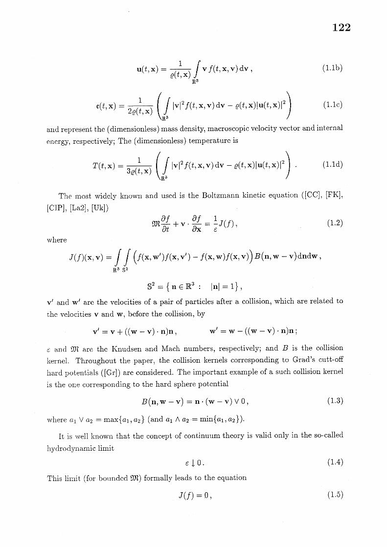
$\mathrm{u}(t, \mathrm{x})=\frac{1}{\rho(t,\mathrm{x})}\int_{\mathrm{R}^{3}}\mathrm{v}f(t, \mathrm{x}, \mathrm{v})\mathrm{d}\mathrm{v}$, (l.lb)
$\mathfrak{e}(t, \mathrm{x})=\frac{1}{2\rho(t,\mathrm{x})}(\int_{\mathrm{J}\mathrm{R}^{3}}|\mathrm{v}|^{2}f(t, \mathrm{x}, \mathrm{v})\mathrm{d}\mathrm{v}-\rho(t, \mathrm{x})|\mathrm{u}(t, \mathrm{x})|^{2})$ (l.lc)
and represent the (dimensionless) mass density, macroscopic velocity vector and internal
energy, respectively; The (dimensionless) temperature is
$T(t, \mathrm{x})=\frac{1}{3\rho(t,\mathrm{x})}(\int_{\mathrm{J}\mathrm{R}^{3}}|\mathrm{v}|^{2}f(t, \mathrm{x}, \mathrm{v})\mathrm{d}\mathrm{v}-\rho(t, \mathrm{x})|\mathrm{u}(t, \mathrm{x})|^{2})$ (l.ld)
The most widely known and used is the Boltzmann kinetic equation $([\mathrm{C}\mathrm{C}],$ $[\mathrm{F}\mathrm{K}]$ ,
[CIP], [La2], [Uk] $)$
$\mathfrak{M}\frac{\partial f}{\partial t}+\mathrm{v}\cdot\frac{\partial f}{\partial \mathrm{x}}=\frac{1}{\epsilon}J(f)$ , (1.2)
where
$J(f)( \mathrm{x}, \mathrm{v})=\int_{\mathrm{J}\mathrm{R}^{3}\mathrm{S}}\int_{2}(f(\mathrm{x}, \mathrm{w}’)f(\mathrm{x}, \mathrm{v}’)-f(\mathrm{x}, \mathrm{w})f(\mathrm{x}, \mathrm{v}))B(\mathrm{n}, \mathrm{w}-\mathrm{v})\mathrm{d}\mathrm{n}\mathrm{d}\mathrm{w}$
,
$\mathrm{S}^{2}=\{\mathrm{n}\in \mathbb{R}^{3} : |\mathrm{n}|=1\}$ ,
$\mathrm{v}’$ and $\mathrm{w}’$ are the velocities of a pair of particles after a collision, which are related to
the velocities $\mathrm{v}$ and $\mathrm{w}$ , before the collision, by
$\mathrm{v}’=\mathrm{v}+((\mathrm{w}-\mathrm{v})\cdot \mathrm{n})\mathrm{n}$ , $\mathrm{w}’=\mathrm{w}-((\mathrm{w}-\mathrm{v})\cdot \mathrm{n})\mathrm{n}$ ;
$\overline{\mathrm{e}}$ and $\mathfrak{M}$ are the Knudsen and Mach numbers, respectively; and $B$ is the collision
kernel. Throughout the paper, the collision kernels corresponding to $\mathrm{G}\mathrm{r}\mathrm{a}\mathrm{d}’ \mathrm{s}$ cutt-off
hard potentials $([\mathrm{G}\mathrm{r}])$ are considered. The important example of a such collision kernel
is the one corresponding to the hard sphere potential
$B(\mathrm{n}, \mathrm{w}-\mathrm{v})=\mathrm{n}\cdot(\mathrm{w}-\mathrm{v})\vee 0$ , (1.3)
where $a_{1} \vee a_{2}=\max\{a_{1}, a_{2}\}$ (and $a_{1} \wedge a_{2}=\min\{a_{1},$ $a_{2}\}$ ).
It is well known that the concept of continuum theory is valid only in the so-called
hydrodynamic limit
$\epsilon\downarrow 0$ . (1.4)
This linlit (for bounded $9\mathfrak{n}$) formally leads to the equation
$J(f)=0$ , (1.5)
122
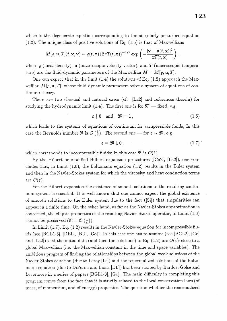
which is the degenerate equation corresponding to the singularly perturbed equation(1.2). The unique class of positive solutions of Eq. (1.5) is that of Maxwellians
$M[ \rho, \mathrm{u}, T](t, \mathrm{x}, \mathrm{v})=\rho(t, \mathrm{x})(2\pi T(t, \mathrm{x}))^{-3/2}\exp(-\frac{|\mathrm{v}-\mathrm{u}(t,\mathrm{x})|^{2}}{2T(t,\mathrm{x})})$ ,
where $\llcorner 0$ (local density), $\mathrm{u}$ (macroscopic velocity vector), and $T$ (macroscopic tempera-ture) $\mathrm{a}\mathrm{l}\cdot \mathrm{e}$ the fluid-dynamic parameters of the Maxwellian $M=M[\rho, \mathrm{u}, T]$ .
One can expect that in the limit (1.4) the solutions of Eq. (1.2) approach the Max-avellian $f\backslash I[\rho, \mathrm{u}, T]$ , whose fluid-dynamic parameters solve a system of equations of con-tinuum theory.
There are two classical and natural cases (cf. [La2] and references therein) forstudying the hydrodynamic limit (1.4). The first one is for $\mathfrak{M}$ –fixed, e.g.
$\epsilon\downarrow 0$ and $\mathfrak{M}=1$ , (1.6)
which leads to the systems of equations of continuum for compressible fluids; In thiscase the $\mathrm{R}\mathrm{e}\mathrm{y}\mathrm{n}\mathrm{o}\mathrm{l}\dot{\mathrm{d}}\mathrm{s}$ number $\Re$ is $\mathcal{O}(\frac{1}{\epsilon})$ . The second one –for $\epsilon\sim \mathfrak{M}$ , e.g.
$\epsilon=\mathfrak{M}\downarrow 0$ , (1.7)
which corresponds to incompressible fluids; In this case $\Re$ is $\mathcal{O}(1)$ .By the Hilbert or modified Hilbert expansion procedures ([Ca2], [La2]), one con-
cludes that, in Limit (1.6), the Boltzmann equation (1.2) results in the Euler systemand then in the Navier-Stokes system for which the viscosity and heat conduction termsare $O’(\epsilon)$ .
For the Hilbert expansion the existence of smooth solutions to the resulting contin-uum system is essential. It is well known that one cannot expect the global existenceof smooth solutions to the Euler system due to the fact ([Si]) that singularities canappear in a finite time. On the other hand, as far as the Navier-Stokes approximation isconcerned, the elliptic properties of the resulting Navier-Stokes operator, in Limit (1.6)cannot be preserved $( \Re=\mathcal{O}(\frac{1}{\epsilon}))$ .
In Limit (1.7), Eq. (1.2) results in the Navier-Stokes equation for incompressible flu-ids (see [BGL1-3], [DEL], [BU], [Go]). In this case one has to assume (see [BGL2], [Go]
and [La2] $)$ that the initial data (and then the solutions) to Eq. (1.2) are $\mathcal{O}(\epsilon)$-close to aglobal Maxwellian (i.e. the Maxwellian constant in the time and space variables). Theambitious program of finding the relationships between the global weak solutions of theNavier-Stokes equation (due to Leray [Le]) and the renormalized solutions of the Boltz-mann equation (due to $\mathrm{D}\mathrm{i}\mathrm{P}\mathrm{e}\mathrm{r}\mathrm{n}\mathrm{a}$ and Lions [DL]) has been started by Bardos, Golse and$\mathrm{L}\mathrm{e}\mathrm{v}\mathrm{e}\mathrm{r}\mathrm{m}\mathrm{o}\mathrm{l}\cdot \mathrm{e}$ in a series of papers [BGL1-3], [Go]. The main difficulty in completing this$\mathrm{p}\mathrm{r}\mathrm{o}\mathrm{g}\mathrm{l}\cdot \mathrm{a}\mathrm{m}$ comes from the fact that it is strictly related to the local conservation laws (ofmass, of momentum, and of energy) properties. The question whether the renormalized
123
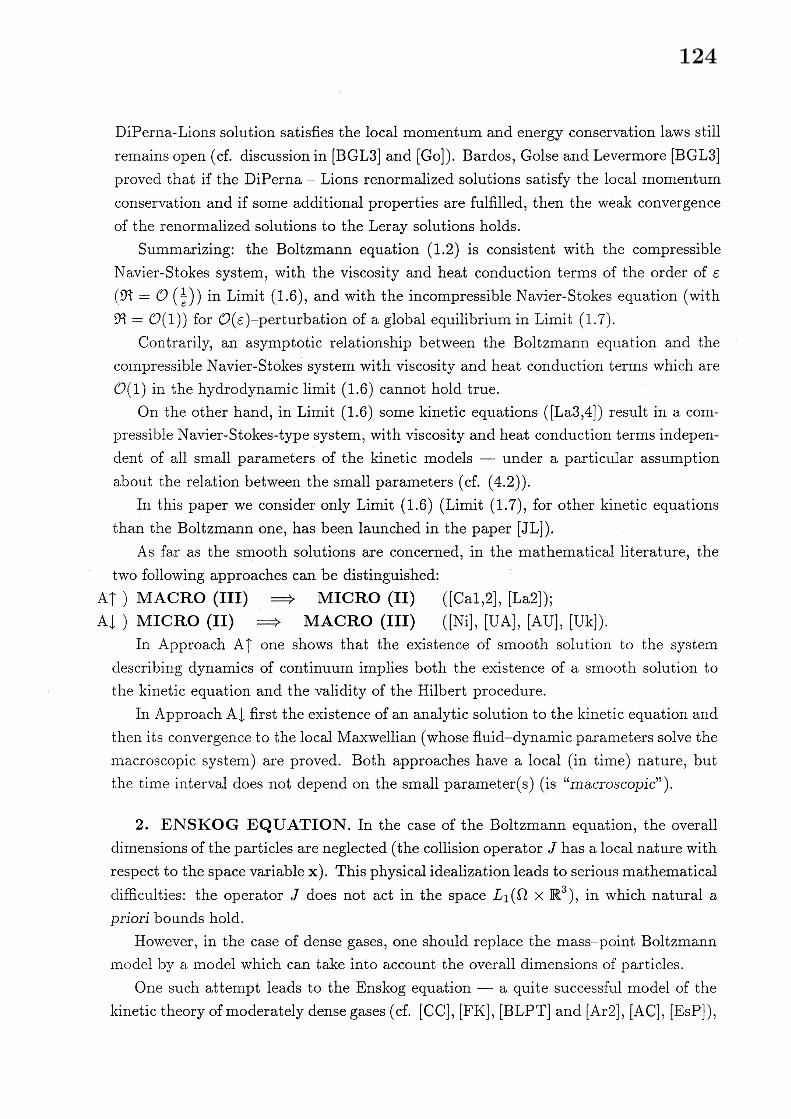
$\mathrm{D}\mathrm{i}\mathrm{P}\mathrm{e}\mathrm{r}\mathrm{n}\mathrm{a}$ -Lions solution satisfies the local momentum and energy conservation laws stillremains open (cf. discussion in [BGL3] and [Go]). Bardos, Golse and Levermore [BGL3]proved that if the $\mathrm{D}\mathrm{i}\mathrm{P}\mathrm{e}\mathrm{r}\mathrm{n}\mathrm{a}$ –Lions renormalized solutions satisfy the local momentumconservation and if some additional properties are fulfilled, then the weak convergenceof the renormalized solutions to the Leray solutions holds.
Summarizing: the Boltzmann equation (1.2) is consistent with the compressibleNavier-Stokes system, with the viscosity and heat conduction terms of the order of $\epsilon$
$( \mathfrak{R}=\mathcal{O}(\frac{1}{\epsilon:}))$ in Limit (1.6), and with the incompressible Navier-Stokes equation (with$\Re=O’(1))$ for $\mathcal{O}(\epsilon)$-perturbation of a global equilibrium in Limit (1.7).
Contrarily, an asymptotic relationship between the Boltzmann equation and thecompressible Navier-Stokes system with viscosity and heat conduction terms which are$\mathcal{O}(1)$ in the hydrodynamic limit (1.6) cannot hold true.
On the other hand, in Limit (1.6) some kinetic equations $([\mathrm{L}\mathrm{a}3,4])$ result in a com-pressible Navier-Stokes-type system, with viscosity and heat conduction terms indepen-dent of all small parameters of the kinetic models –under a particular assumptionabout the relation between the small parameters (cf. (4.2)).
In this paper we consider only Limit (1.6) (Limit (1.7), for other kinetic equationsthan the Boltzmann one, has been launched in the paper [JL] $)$ .
As far as the smooth solutions are concerned, in the mathematical literature, thetwo following approaches can be distinguished:
$\mathrm{A}\uparrow)$ MACRO (III) $\Rightarrow$ MICRO (II) ( $[\mathrm{C}\mathrm{a}1,2]$ , [La2]);$\mathrm{A}\downarrow)$ MICRO (II) $\Rightarrow$ MACRO (III) ([Ni], [UA], [AU], [Uk]).
In Approach $\mathrm{A}\uparrow \mathrm{o}\mathrm{n}\mathrm{e}$ shows that the existence of smooth solution to the systemdescribing dynamics of continuum implies both the existence of a $\mathrm{s}\mathrm{m}\mathrm{o}(\supset \mathrm{t}\mathrm{h}$ solution tothe kinetic equation and the validity of the Hilbert procedure.
In Approach $\mathrm{A}\downarrow \mathrm{f}\mathrm{i}\mathrm{r}\mathrm{s}\mathrm{t}$ the existence of an analytic solution to the kinetic equation andthen its convergence to the local Maxwellian (whose fluid-dynamic parameters solve themacroscopic system) are proved. Both approaches have a local (in time) nature, butthe time interval does not depend on the small parameter(s) (is “macroscopic”).
2. ENSKOG EQUATION. In the case of the Boltzmann equation, the overalldimensions of the particles are neglected (the collision operator $J$ has a local nature withrespect to the space variable x). This physical idealization leads to serious mathematicaldifficulties: the operator $J$ does not act in the space $L_{1}(\Omega\cross \mathbb{R}^{3})$ , in which natural $a$
priori bounds hold.However, in the case of dense gases, one should replace the mass-point Boltzmann
lnodel by a model which can take into account the overall dimensions of particles.One such attempt leads to the Enskog equation –a quite successful model of the
kinetic theory of moderately dense gases (cf. [CC], [FK], [BLPT] and [Ar2], [AC], $[\mathrm{E}\mathrm{s}\mathrm{P}]$ ),
124
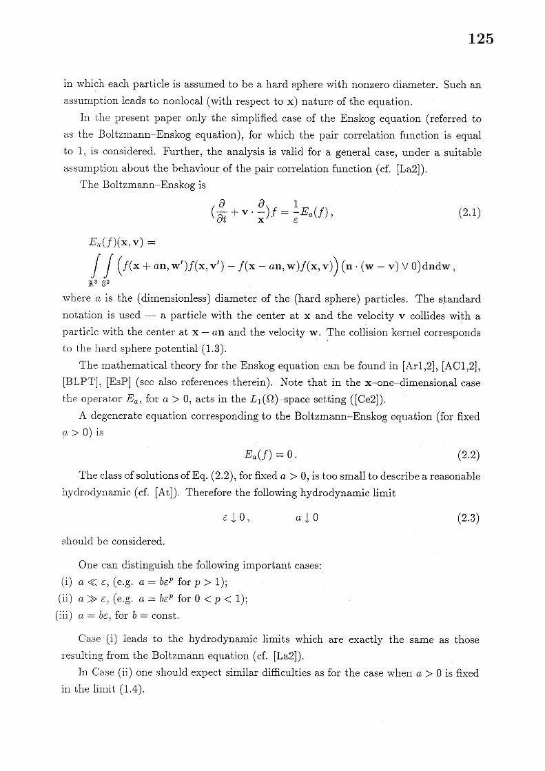
in which each particle is assumed to be a hard sphere with nonzero diameter. Such anassumption leads to nonlocal (with respect to x) nature of the equation.
In the present paper only the simplified case of the Enskog equation (referred toas the Boltzmann-Enskog equation), for which the pair correlation function is equalto 1, is considered. Further, the analysis is valid for a general case, under a suitableassumption about the behaviour of the pair correlation function (cf. [La2]).
The Boltzmann-Enskog is
$( \frac{\partial}{\partial t}+\mathrm{v}\cdot\frac{\partial}{\mathrm{x}})f=\frac{1}{\epsilon}E_{a}(f)$ , (2.1)
$E_{a}(f.)(\mathrm{x}, \mathrm{v})=$
$\int_{\mathrm{R}^{3}\mathrm{S}}\int_{2}(f(\mathrm{x}+a\mathrm{n}, \mathrm{w}’)f(\mathrm{x}, \mathrm{v}’)-f(\mathrm{x}-a\mathrm{n}, \mathrm{w})f(\mathrm{x}, \mathrm{v}))(\mathrm{n}\cdot(\mathrm{w}-\mathrm{v})\vee 0)\mathrm{d}\mathrm{n}\mathrm{d}\mathrm{w}$,
where $a$ is the (dimensionless) diameter of the (hard sphere) particles. The standardnotation is used –a particle with the center at $\mathrm{x}$ and the velocity $\mathrm{v}$ collides with aparticle with the center at $\mathrm{x}-a\mathrm{n}$ and the velocity $\mathrm{w}$ . The collision kernel correspondsto the hard sphere potential (1.3).
The mathematical theory for the Enskog equation can be found in [Arl,2], [AC1,2],$[\mathrm{B}\mathrm{L}\mathrm{P}\mathrm{T}]_{i}[\mathrm{E}\mathrm{s}\mathrm{P}]$ (see also references therein). Note that in the $\mathrm{x}-\mathrm{o}\mathrm{n}\mathrm{e}$-dimensional casethe operator $E_{a}$ , for $a>0$ , acts in the $L_{1}(\Omega)$-space setting $([\mathrm{C}\mathrm{e}2])$ .
A degenerate equation corresponding to the Boltzmann-Enskog equation (for fixed$a>0)$ is
$E_{a}(f)=0$ . (2.2)
The class of solutions of Eq. (2.2), for fixed $a>0$ , is too small to describe a reasonablehydrodynamic (cf. [At]). Therefore the following hydrodynamic limit
$\overline{\mathrm{c}}\downarrow 0$ , $a\downarrow 0$ (2.3)
should be considered.
One can distinguish the following important cases:(i) $a\ll\epsilon$ , (e.g. $a=b\epsilon^{p}$ for $p>1$ );(ii) $a\gg\epsilon$ , (e.g. $a=b\epsilon^{p}$ for $0<p<1$ );(iii) $a=b\epsilon$ , for $b=\mathrm{c}\mathrm{o}\mathrm{n}\mathrm{s}\mathrm{t}$ .
Case (i) leads to the hydrodynamic limits which are exactly the same as thoseresulting from the Boltzmann equation (cf. [La2]).
In $\mathrm{C}^{1}\prime \mathrm{a}\mathrm{s}\mathrm{e}(\mathrm{i}\mathrm{i})$ one should expect similar difficulties as for the case when $a>0$ is fixedin the lilluit (1.4).
125
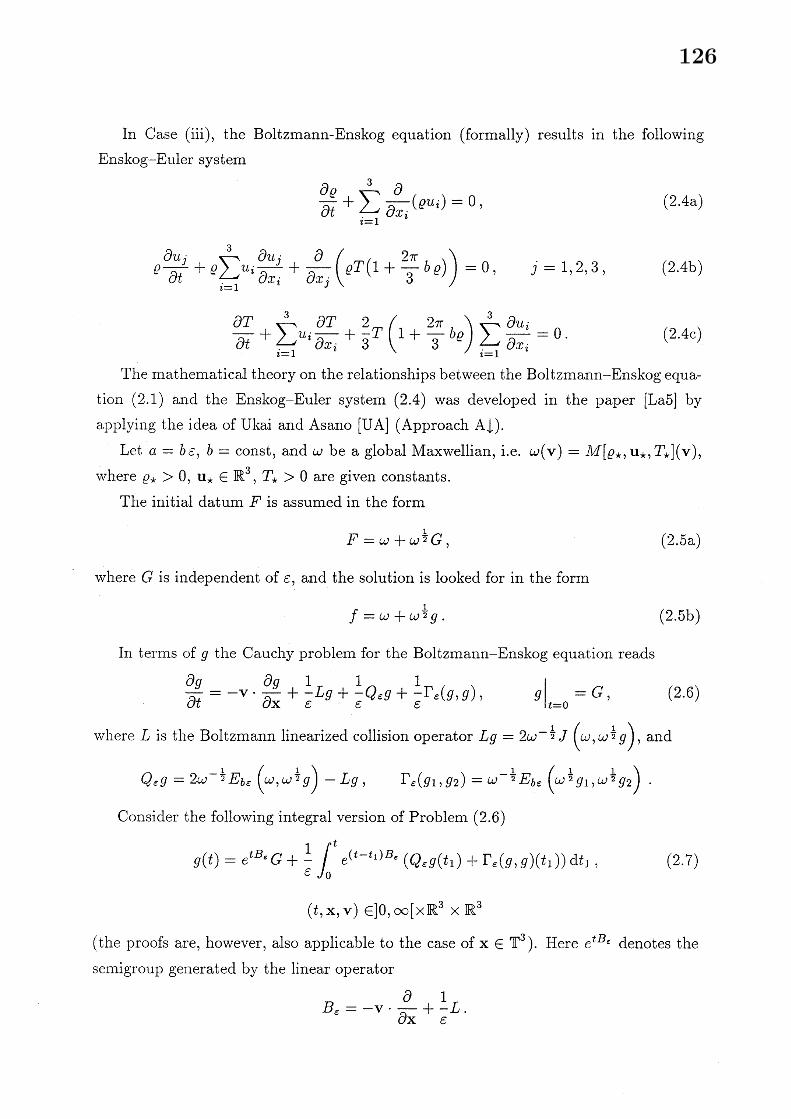
In Case (iii), the Boltzmann-Enskog equation (formally) results in the followingEnskog-Euler system
$\frac{\partial\rho}{\partial t}+\sum_{i=1}^{3}\frac{\partial}{\partial x_{i}}(\rho u_{i})=0$ , (2.4a)
$\rho\frac{\partial u_{j}}{\partial t}+\rho\sum_{i=1}^{3}u_{i^{\frac{\partial u_{j}}{\partial x_{i}}}}+\frac{\partial}{\partial x_{j}}(\rho T(1+\frac{2\pi}{3}b\rho))=0$ , $j=1,2,3$ , (2.4b)
$\frac{\partial T}{\partial t}+\sum_{i=1}^{3}u_{i}\frac{\partial T}{\partial x_{i}}+\frac{2}{3}T(1+\frac{2\pi}{3}b\rho)\sum_{i=1}^{3}\frac{\partial u_{i}}{\partial x_{i}}=0$ . (2.4c)
The mathematical theory on the relationships between the Boltzmann-Enskog equa-tion (2.1) and the Enskog-Euler system (2.4) was developed in the paper [La5] byapplying the idea of Ukai and Asano [UA] (Approach $\mathrm{A}\downarrow$ ).
Let $a=b\epsilon,$ $b=\mathrm{c}\mathrm{o}\mathrm{n}\mathrm{s}\mathrm{t}$ , and $\omega$ be a global Maxwellian, i.e. $\omega(\mathrm{v})=M[\rho_{\star}, \mathrm{u}_{\star}, T_{\star}](\mathrm{v})$ ,where $\rho_{\star}>0,$ $\mathrm{u}_{\star}\in \mathbb{R}^{3},$ $T_{\star}>0$ are given constants.
The initial datum $F$ is assumed in the form
$F=\omega+\omega^{\frac{1}{2}}G$ , (2.5a)
where $C_{\tau}$ is independent of $\epsilon$ , and the solution is looked for in the form
$f=\omega+\omega^{\frac{1}{2}}g$ . (2.5b)
In $\mathrm{t}\mathrm{e}\mathrm{l}\cdot \mathrm{m}\mathrm{s}$ of $g$ the $\mathrm{C}^{\mathrm{t}}\mathrm{a}\mathrm{u}\mathrm{c}\mathrm{h}\mathrm{y}$ problem for the Boltzmann-Enskog equation reads
$\frac{\partial g}{\partial t}=-\mathrm{v}\cdot\frac{\partial g}{\partial \mathrm{x}}+\frac{1}{\epsilon}Lg+\frac{1}{\epsilon}Q_{\text{\’{e}}:}g+\frac{1}{\epsilon}\Gamma_{\epsilon}(g, g)$ , $g|_{t=0}=G$ , (2.6)
where $L$ is the Boltzmann linearized collision operator $Lg=2\omega^{-\frac{1}{2}}J(\omega,\omega^{\frac{1}{2}}g)$ , and
$Q_{\xi j}g=2\omega^{-\frac{1}{2}}E_{b\epsilon}(\omega,\omega^{\frac{1}{2}}g)-Lg$ , $\Gamma_{\epsilon}(g_{1}, g_{2})=\omega^{-\frac{1}{2}}E_{b\text{\’{e}}:}(\omega^{\frac{1}{2}}g_{1},$ $\omega^{\frac{1}{2}}g_{2})$
Consider the following integral version of Problem (2.6)
$g(t)=e^{tB_{\epsilon}}G+ \frac{1}{\epsilon}\int_{0}^{t}e^{(t-t_{1})B_{\epsilon}}(Q_{\epsilon}g(t_{1})+\Gamma_{\epsilon}(g, g)(t_{1}))\mathrm{d}t_{1}$ , (2.7)
$(t, \mathrm{x}, \mathrm{v})\in]0,$ $\infty[\cross \mathbb{R}^{3}\cross \mathbb{R}^{3}$
(the proofs are, however, also applicable to the case of $\mathrm{x}\in \mathbb{T}^{3}$ ). Here $e^{tB_{\epsilon}}$ denotes thesemigroup generated by the linear operator
$B \text{\’{e}}:=-\mathrm{v}\cdot\frac{\partial}{\partial \mathrm{x}}+\frac{1}{\epsilon}L$ .
126

Let $\mathrm{B}^{\alpha}$ denote the space equipped with the norm
$||g||^{(\alpha)}= \sup_{\mathrm{v}\in \mathrm{R}^{3}}|\langle \mathrm{v}\rangle^{\alpha}g(\mathrm{v})|$ , $\alpha\in \mathbb{R}^{1}$ ,
where $\langle \mathrm{v}\rangle^{\alpha}=(1+|\mathrm{v}|)^{\alpha}$ and $\alpha\in \mathbb{R}^{1}$ . Let $\hat{g}=Fg$ denote the Fourier transform of a
function $g\in S’(\mathbb{R}^{3}\cross \mathbb{R}^{3})$ with respect to the position variable $\mathrm{x}$ ,
$\hat{g}(\mathrm{k}, \mathrm{v})=Fg(\mathrm{k}, \mathrm{v})=\frac{1}{(2\pi)^{3/2}}\int_{\mathrm{J}\mathrm{R}^{3}}e^{-i\mathrm{k}\cdot \mathrm{x}}g(\mathrm{x}, \mathrm{v})\mathrm{d}\mathrm{x}$, $\mathrm{k}\in \mathbb{R}^{3}$
Let $\mathrm{X}_{\beta,\gamma}^{(0)}$ be the space equipped with the norm
$||g||_{\beta,\gamma}^{(\alpha)}= \sup_{\mathrm{k},\mathrm{v}\in \mathrm{J}\mathrm{R}^{3}}|\langle \mathrm{v}\rangle^{\alpha}\langle \mathrm{k}\rangle^{\beta}\exp(\gamma|\mathrm{k}|)\hat{g}(\mathrm{k}, \mathrm{v})|$ , $\alpha,$$\beta,$ $\gamma\in \mathbb{R}_{+}^{1}$ ,
$\alpha,$$\beta,$
$\gamma$ are positive constants.The space $\dot{\mathrm{X}}_{\beta,\gamma}^{(\alpha)}$ is a closed subspace of $\mathrm{X}_{\beta,\gamma}^{(\alpha)}$ , such that
$g\in\dot{\mathrm{X}}_{\theta,\gamma}^{(\alpha)}$$\Leftrightarrow$ $g\in \mathrm{X}_{\beta,\gamma}^{(\alpha)}$ &llF $(\chi(|\mathrm{k}|+|\mathrm{v}|>\xi)\hat{g}(\mathrm{k}, \mathrm{v}))||_{\beta,\gamma}^{(\alpha)}arrow 0$ , as $\xiarrow\infty$ ,
where $\chi(\mathrm{t}\mathrm{r}\mathrm{u}\mathrm{t}\mathrm{h})=1$ and $\chi(\mathrm{f}\mathrm{a}\mathrm{l}\mathrm{s}\mathrm{e})=0$ .For $\eta\geq 0$ and an interval $I\subset \mathbb{R}^{1}$ , let
$\mathrm{Y}_{\beta,\gamma}^{\alpha,\eta}(I)=\{g=g(t)$ : $\tilde{g}_{\eta}\in C_{B}^{0}(I;\dot{\mathrm{X}}_{\beta,\gamma}^{(\alpha)});\tilde{g}_{\eta}(t, \mathrm{x}, \mathrm{v})\equiv F^{-1}\exp(-\eta t|\mathrm{k}|)\hat{g}(t, \mathrm{k}, \mathrm{v})\}$
be the space equipped with the norm
$||g||_{\beta,\gamma,I}^{\alpha,\eta}= \sup_{t\in I}||g(t)||_{\beta,\gamma-\eta t}^{(\alpha)}$ .
Let
$\mathbb{Z}_{\beta,\gamma,t_{0}}^{\alpha,\eta,1}=C_{B}^{0}(]0,1];\mathrm{Y}_{\beta_{)}\gamma}^{\alpha,\eta}([0, t_{0}]))$
be the Banach space of $\epsilon$-dependent functions, equipped with the norm
$||g||_{\beta,\gamma,t_{0}}^{\alpha,\eta,1}=0 \leq t\leq t_{0}0<\epsilon\leq 1\sup||g(t)||_{\beta,\gamma-\eta t}^{(\alpha)}$
.
Let
$\hat{B}_{\epsilon}(\mathrm{k})\hat{g}(\mathrm{k}, \mathrm{v})\equiv \mathcal{F}B_{\epsilon}g(\mathrm{k}, \mathrm{v})\equiv\hat{g}(\mathrm{k}, \mathrm{v})$ .
The semigroup $\frac{1}{\epsilon}e^{t\hat{B}_{\epsilon}(\mathrm{k})}$ is such that ( $[\mathrm{E}\mathrm{l}\mathrm{P}]$ , [Uk], [Anl,3])
$e^{t\hat{B}_{\epsilon}(\mathrm{k})}= \chi(\epsilon|\mathrm{k}|\leq\kappa)\sum e^{\lambda_{j}^{\epsilon}(\mathrm{k})t}P_{j}^{\epsilon}(\mathrm{k})4+U_{\epsilon}(t, \mathrm{k})$ ,$j=0$
where $\kappa$ is a positive constant; $\lambda_{j}^{\epsilon}\in C^{\infty}([-\kappa, \kappa])$ (for $j=0,$ $\ldots,$
$4$ ) are such that
127
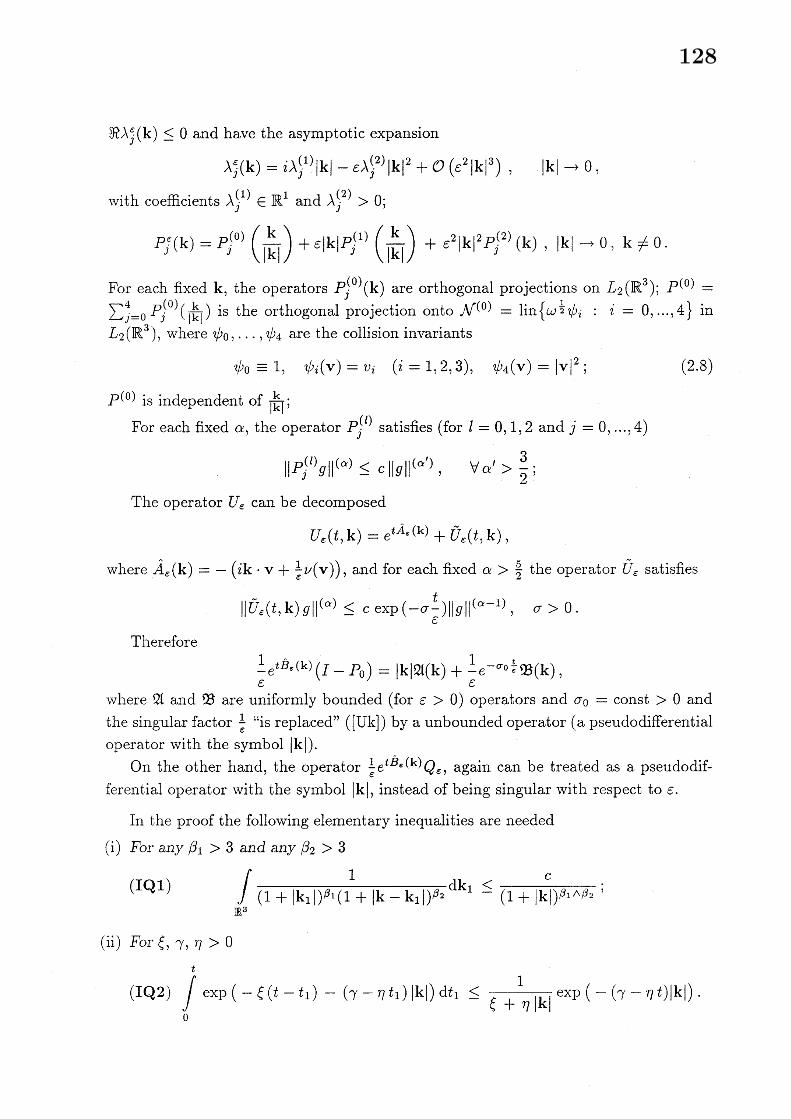
$\Re,\backslash _{\check{j}}^{\epsilon}(\mathrm{k})\leq 0$ and have the asymptotic expansion
$\lambda_{j}^{\epsilon}(\mathrm{k})=i\lambda_{j}^{(1)}|\mathrm{k}|-\epsilon\lambda_{j}^{(2)}|\mathrm{k}|^{2}+\mathcal{O}(\epsilon^{2}|\mathrm{k}|^{3})$ , $|\mathrm{k}|arrow 0$ ,
with coefficients $\lambda_{j}^{(1)}\in \mathbb{R}^{1}$ and $\lambda_{j}^{(2)}>0$ ;
$P_{j}^{\epsilon}( \mathrm{k})=P_{j}^{(0)}(\frac{\mathrm{k}}{|\mathrm{k}|})+\epsilon|\mathrm{k}|P_{j}^{(1)}(\frac{\mathrm{k}}{|\mathrm{k}|})+\epsilon^{2}|\mathrm{k}|^{2}P_{j}^{(2)}(\mathrm{k}),$ $|\mathrm{k}|arrow 0,$ $\mathrm{k}\neq 0$ .
For each fixed $\mathrm{k}$ , the operators $P_{j}^{(0)}(\mathrm{k})$ are orthogonal projections on $L_{2}(\mathbb{R}^{3});P^{(0)}=$
$\sum_{j=0}^{4}P_{j}^{(0)}(\frac{\mathrm{k}}{|\mathrm{k}|})$ is the orthogonal projection onto $N^{(0)}=\mathrm{l}\mathrm{i}\mathrm{n}\{\omega^{\frac{1}{2}}\psi_{i} : i=0, \ldots, 4\}$ in$L_{2}(\mathbb{R}^{3})$ , where $\psi_{0},$
$\ldots,$$\psi_{4}$ are the collision invariants
$\psi_{0}\equiv 1$ , $\psi_{i}(\mathrm{v})=v_{i}$ $(i=1,2,3)$ , $\psi_{4}(\mathrm{v})=|\mathrm{v}|^{2}$ ; (2.8)
$P^{(0)}$ is independent of $\frac{\mathrm{k}}{|\mathrm{k}|}$ ;
For each fixed $\alpha$ , the operator $P_{j}^{(l)}$ satisfies (for $l=0,1,2$ and $j=0,$ $\ldots,$
$4$ )
$||P_{j}^{(l)}g||^{(\alpha)}\leq c||g||^{(\alpha’)}$ , $\forall\alpha’>\frac{3}{2}$ ;
The operator $U_{\epsilon}$ can be decomposed
$U_{\text{\’{e}} \mathrm{i}}(t, \mathrm{k})=e^{t\hat{A}_{\epsilon}(\mathrm{k})}+\tilde{U}_{\epsilon}(t, \mathrm{k})$ ,
where $\hat{A}_{\epsilon}(\mathrm{k})=-(i\mathrm{k}\cdot \mathrm{v}+\frac{1}{e}\nu(\mathrm{v}))$ , and for each fixed $\alpha>\frac{5}{2}$ the operator $\tilde{U}_{\epsilon}$ satisfies
$|| \tilde{U}_{\epsilon}(t, \mathrm{k})g||^{(\alpha)}\leq c\exp(-\sigma\frac{t}{\epsilon})||g||^{(\alpha-1)}$ , $\sigma>0$ .Therefore
$\frac{1}{\epsilon}e^{t\hat{B}_{\epsilon}(\mathrm{k})}(I-P_{0})=|\mathrm{k}|\mathfrak{U}(\mathrm{k})+\frac{1}{\epsilon}e^{-\sigma_{0}\frac{t}{\epsilon}}\mathfrak{B}(\mathrm{k})$ ,
where $\mathfrak{U}$ and $\mathfrak{B}$ are uniformly bounded (for $\epsilon>0$ ) operators and $\sigma_{0}=\mathrm{c}\mathrm{o}\mathrm{n}\mathrm{s}\mathrm{t}>0$ andthe singular factor $\frac{1}{\epsilon}$ “is replaced” $([\mathrm{U}\mathrm{k}])$ by a unbounded operator (a pseudodifferentialoperator with the symbol $|\mathrm{k}|$ ).
On the other hand, the operator $\frac{1}{\epsilon}e^{t\dot{B}_{\epsilon}(\mathrm{k})}Q_{\epsilon}$ , again can be treated as a pseudodif-ferential operator with the symbol $|\mathrm{k}|$ , instead of being singular with respect to $\epsilon$ .
In the proof the following elementary inequalities are needed
(i) For any $\beta_{1}>3$ and any $\beta_{2}>3$
$(\mathrm{I}\mathrm{Q}1)$
$\int_{\mathrm{J}\mathrm{R}^{3}}\frac{1}{(1+|\mathrm{k}_{1}|)^{\beta_{1}}(1+|\mathrm{k}-\mathrm{k}_{1}|)^{\beta_{2}}}\mathrm{d}\mathrm{k}_{1}\leq\frac{c}{(1+|\mathrm{k}|)^{\beta_{1}\wedge\beta_{2}}}$;
(ii) For $\xi,$$\gamma,$ $\eta>0$
$( \mathrm{I}\mathrm{Q}2)\int_{0}^{t}\exp(-\xi(t-t_{1})-(\gamma-\eta t_{1})|\mathrm{k}|)\mathrm{d}t_{1}\leq\frac{1}{\xi+\eta|\mathrm{k}|}\exp(-(\gamma-\eta t)|\mathrm{k}|)$ .
128

The main result of the paper [La5] is
THEOREM 2.1. Let $\alpha,$$\beta,$
$\gamma,$$b,$
$\eta$ and $t_{0}$ be properly chosen (independent of $\epsilon$ ). Ifthe initial data
. $(\alpha)$
$G\in \mathrm{X}_{\beta,\gamma}$ (2.9a)
satisfies the smalln$ess$ condition
$||G||_{\beta,\gamma}^{(\alpha)}<\theta_{0}$ , (2.9b)
where $\theta_{0}$ is a gicen $co\mathrm{n}$siant.Tben
$(i.)$ ther$e$ exists a unique classical $sol\mathrm{u}t\mathrm{i}$on $g$ of the Cauchy problem for the Boltzmann-$Ens\mathrm{A}og$ equation (2.1) on $t\mathrm{A}e$ time interval $[0, i_{0}]$ , such tbat
$g\in \mathbb{Z}_{\beta,\gamma,t_{0}}^{\alpha,\eta,1}$ , (2.10)
$\frac{\partial}{\partial t}g\in C^{0}(]0,1];\mathrm{Y}_{\beta-1,\gamma}^{\alpha-1,\eta}([0, t_{0}]))$ . (2.11)
(ii) $g(t)arrow g_{0}(t)$ , as $\epsilon\downarrow 0$ , strongly in $\mathrm{Y}_{\beta,\gamma}^{\alpha,\eta}([\delta, t_{0}])$ , for any $\delta\in$ ] $0,$ $t_{0}$ [;$(\mathrm{i}\mathrm{i}\mathrm{i})\backslash f_{\mathrm{U}}(t)=\omega+\omega^{\frac{1}{2}}g_{0}(t)$ is the Maxwellian such that $(\rho, \mathrm{u}, T)$ is a classical solution of
the Cauchy problem for the Enskog-Euler sysiem (2.4) wiih the initial data
$\rho|_{t=0}=(\psi_{0}, F)_{L_{2}(\mathrm{R}^{3})}$ , $T|_{t=0}=(\psi_{4}, F)_{L_{2}(\mathrm{R}^{3})}$ , (2.12a)
$u_{j}|_{t=0}=(\psi_{j}, F)_{L_{2}(\mathit{1}\mathrm{R}^{3})}$ , $j=1,2,3$ . (2.12b)
As a by-product, Theorem 2.1 delivers an existence result for the Enskog-Eulersystem (2.4). For the Euler system (i.e. for $b=0$ ), which is a symmetric hyperbolicsystem provided that $\rho>0$ , the (local) existence and uniqueness theorem is availablefor the Cauchy problem with analytical initial data $(\rho, \mathrm{u}, T)|_{t=0}$ such that
$\rho|_{t=0}>0$ . (2.13)
This assumption was essential in the proof by Nishida [Ni] of the convergence of solutionof the $\mathrm{B}(\supset \mathrm{l}\mathrm{t}\mathrm{z}\mathrm{m}\mathrm{a}\mathrm{n}\mathrm{n}$ equation to the Maxwellian, which fluid-dynamic parameters solvethe Euler system. This type of assumption was also essential in the methods reviewedin the lecture [La2]. On the other hand, Assumption (2.13) was removed in methods$\rceil_{)}\mathrm{y}$ Ulcai and Asano [UA]. It is not necessary either in the paper [La5]. To author’sknowledge, the existence result, which follows from Theorem 2.1, is the first for theEnskog-Euler system.
Like for the Boltzmann equation $([\mathrm{U}\mathrm{A}])$ , when the initial layer vanishes, i.e. for
$g_{0}=P^{(0)}g_{0}$ , (2.14)
129

Theorem 2.1 (ii) holds with $\delta=0$ .
3. STOCHASTIC KINETIC EQUATION. A lar$g\mathrm{e}$ number of particle limitfor a system of stochastic particles ([LP], [Lal], and [Cel], [Sk], [An2,3], [Vo]) leads tothe stochastic kinetic equation
$( \frac{\partial}{\partial t}+\mathrm{v}\cdot\frac{\partial}{\partial \mathrm{x}})f=\frac{1}{\epsilon}S(f)$ , (3. 1)
where$S(f)(\mathrm{x}, \mathrm{v})=$
$\int_{\mathrm{I}\mathrm{R}^{3}\Omega}f(f(\mathrm{y}, \mathrm{w}^{*})f(\mathrm{x}, \mathrm{v}^{*})B(\mathrm{y}-\mathrm{x}, \mathrm{w}-\mathrm{v})-f(\mathrm{y}, \mathrm{w})f(\mathrm{x}, \mathrm{v})B(\mathrm{x}-\mathrm{y}, \mathrm{w}-\mathrm{v}))$dydw,
the velocities $\mathrm{v}^{*}$ and $\mathrm{w}^{*}$ are functions of $\mathrm{v}$ and $\mathrm{w}$ as well as of the distance betweenthe two particles $\mathrm{y}-\mathrm{x}$ , according to
$\mathrm{v}^{*}=\mathrm{v}+((\mathrm{w}-\mathrm{v})\cdot \mathrm{n})\mathrm{n}$ , $\mathrm{w}^{*}=\mathrm{w}-((\mathrm{w}-\mathrm{v})\cdot \mathrm{n})\mathrm{n}$ , (3.2)
where now
$\mathrm{n}=\frac{\mathrm{y}-\mathrm{x}}{|\mathrm{y}-\mathrm{x}|}$ , for $\mathrm{y}\neq \mathrm{x}$ , $\mathrm{y},$$\mathrm{x}\in\Omega$ ,
$B$ is such that (cf. [Cel], [LP], [Lal])
$B(\mathrm{x}, \mathrm{v})=0$ for $\mathrm{x}\cdot \mathrm{v}<0$ , $\forall \mathrm{x}\in\Omega,$$\mathrm{v}\in \mathbb{R}^{3}$ (3.3)
In this Section it is assumed that (cf. [La4])
$B( \mathrm{x}, \mathrm{v})=\frac{3}{R^{3}-r^{3}}\chi(r\leq|\mathrm{x}|\leq R)\chi(\mathrm{x}, \mathrm{v}\geq 0)B(\frac{\mathrm{x}}{|\mathrm{x}|}, \mathrm{v})$ , (3.4)
where $0<r<R<\infty$ and $B$ is the collision kernel corresponding to $\mathrm{G}\mathrm{r}\mathrm{a}\mathrm{d}’ \mathrm{s}$ cut-offhard potentials.
Equation (3.1) can also be considered in the symmetrized form ([Mo], [Po], [BP]),i.e. when Assumption (3.3) is replaced by
$B(-\mathrm{x}, \mathrm{v})=B(\mathrm{x}, \mathrm{v})$ , $\forall \mathrm{x}\in\Omega$ $\forall \mathrm{v}\in \mathbb{R}^{3}$ (3.5)
The two assumptions (3.3) and (3.5) lead to different hydrodynamic limits $([\mathrm{L}\mathrm{a}3,4])$ .Case (3.5) is discussed in Section 4.
Note that Eq. (3.1) formally leads to the Boltzmann equation for
$B( \mathrm{x}, \mathrm{v})=\delta(\mathrm{x})\chi(\mathrm{x}\cdot \mathrm{v}\geq 0)B(\frac{\mathrm{x}}{|\mathrm{x}|}, \mathrm{v})$ . (3.6)
and therefore Eq. (3.1) can be regarded as a modification (mollification) of the Boltz-mann equation (1.2). A mollified kinetic equation was first proposed by Morgenstern[Mo] and, more generally, by Povzner [Po].
130

Equation (3.1) is referred to as the stochastic kinetic equation (or Povzner equation).
Actually, Povzner considered Eq. (3.1) assuming (3.5). Under the same assumption aclass of more general equations was investigated by Bellomo and Polewczak [BP].
One can expect that the solutions of Eq. (3.1) with (3.4), in the limit $r<R\downarrow \mathrm{O}$
(and for fixed $\epsilon>0$ ), approach the corresponding solution to the Boltzmann equa-
tion (1.2). In fact $([\mathrm{A}\mathrm{C}2])$ , in the limit $a\downarrow \mathrm{O}$ , the solutions of the Boltzmann-Enskogequation (2.1) converge to the $(\mathrm{D}\mathrm{i}\mathrm{P}\mathrm{e}\mathrm{r}\mathrm{n}\mathrm{a}-\mathrm{L}\mathrm{i}\mathrm{o}\mathrm{n}\mathrm{s}-[\mathrm{D}\mathrm{L}])$ renormalized solutions of theBoltzmann equation. The same certainly should be true for the convergence of the
solutions of Eq. (3.1).
On the other hand, in the limit $r\uparrow R$ (where both $R=a>0$ and $\epsilon>0$ remainfixed) the solution of Eq. (3.1) with (3.4) should approach the corresponding solution
of the Boltzmann-Enskog equation (2.1).
Equation (3.1) has nice mathematical properties, which are lacking for the Boltz-
lnann equation (1.2): the collision operator $S$ acts in the space $L_{1}(\Omega)$ . ThereforeEq. (3.1) preserves some mathematical properties of the space homogeneous Boltzmannequation. In particular, the existence of unique smooth global solutions is known ([Mo],
[Po], [An3], [Lal], [BP] $)$ .
The theory of hydrodynamic limits for Eq. (3.1) was proposed in [La3,4].
Different relations between the small parameters $\epsilon$ and $R$ can lead to different hy-
drodynamic equations analogously with the Boltzmann-Enskog case.
If
$R=b\epsilon$ , $b=\mathrm{c}\mathrm{o}\mathrm{n}\mathrm{s}\mathrm{t}$ , (3.7)
then Eq. (3.1) results in the following Euler-type system
$\frac{\partial\rho}{\partial t}+\sum_{i=1}^{3}\frac{\partial}{\partial x_{i}}(\rho u_{i})=0$ , (3.8a)
$\rho\frac{\partial u_{j}}{\partial t}+\rho\sum_{i=1}^{3}u_{i}\frac{\partial u_{j}}{\partial x_{i}}+\frac{\partial}{\partial x_{j}}(\rho T)+b\sum_{i=1}^{3}\frac{\partial}{\partial x_{i}}(\rho^{2}\mathfrak{p}_{ij}(T))=0$ , $j=1,2,3$ , (3.8b)
$\frac{\partial T}{\partial t}+\sum_{i=1}^{3}u_{i}\frac{\partial T}{\partial x_{i}}+\frac{2}{3}T\sum_{i=1}^{3}\frac{\partial u_{i}}{\partial x_{i}}+\frac{2}{3}b\rho\sum_{i,j=1}^{3}\mathfrak{p}_{ij}(T)\frac{\partial u_{j}}{\partial x_{i}}=0$ (3.8c)
where
$\mathrm{p}_{ij}(T)=$
$\frac{\sqrt{2T}}{2\pi^{3}}\int_{\mathrm{R}^{3}\mathrm{R}}\int_{\mathrm{s}3}\int_{2}n_{i}n_{j}(\mathrm{n}\cdot(\mathrm{w}-\mathrm{v})\vee \mathrm{O})B(\mathrm{n}, \sqrt{2T}(\mathrm{w}-\mathrm{v}))\exp(-|\mathrm{v}|^{2}-|\mathrm{w}|^{2})$dn dw $\mathrm{d}\mathrm{v}$ .
131
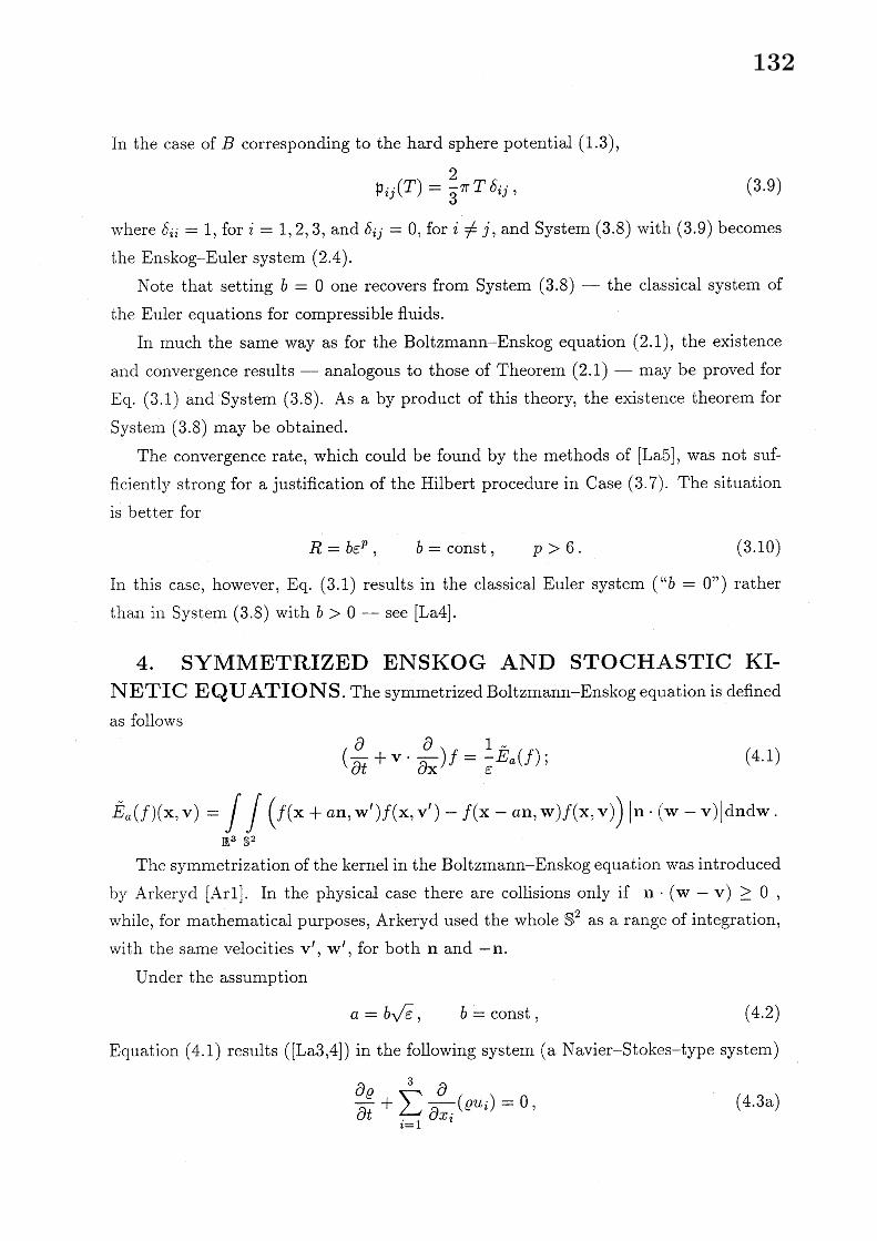
In the case of $B$ corresponding to the hard sphere potential (1.3),
$\mathfrak{p}_{ij}(T)=\frac{2}{3}\pi T\delta_{ij}$ , (3.9)
where $\delta_{ii}=1$ , for $i=1,2,3$ , and $\delta_{ij}=0$ , for $i\neq j$ , and System (3.8) with (3.9) becomes
the Enskog-Euler system (2.4).
Note that setting $b=0$ one recovers from System (3.8) –the classical system of
the Euler equations for compressible fluids.
In much the same way as for the Boltzmann-Enskog equation (2.1), the existence
and convergence results –analogous to those of Theorem (2.1) –may be proved for
Eq. (3.1) and System (3.8). As a by product of this theory, the existence theorem for
System (3.8) may be obtained.
The convergence rate, which could be found by the methods of [La5], was not suf-
ficiently strong for a justification of the Hilbert procedure in Case (3.7). The situation
is better for
$R=b\epsilon^{p}$ , $b=\mathrm{c}\mathrm{o}\mathrm{n}\mathrm{s}\mathrm{t}$ , $p>6$ . (3.10)
In this case, however, Eq. (3.1) results in the classical Euler system $(” b=0”)$ rather
than in System (3.8) with $b>0$ –see [La4].
4. SYMMETRIZED ENSKOG AND STOCHASTIC KI-NETIC EQUATIONS. The symmetrized Boltzmann-Enskog equation is defined
as follows
$( \frac{\partial}{\partial t}+\mathrm{v}\cdot\frac{\partial}{\partial \mathrm{x}})f=\frac{1}{\epsilon}\tilde{E}_{a}(f)_{\mathrm{i}}$ (4.1)
$\tilde{E}_{a}(f)(\mathrm{x}, \mathrm{v})=\int_{\mathrm{J}\mathrm{R}^{3}\mathrm{S}}\int_{2}(f(\mathrm{x}+a\mathrm{n}, \mathrm{w}’)f(\mathrm{x}, \mathrm{v}’)-f(\mathrm{x}-a\mathrm{n}, \mathrm{w})f(\mathrm{x}, \mathrm{v}))|\mathrm{n}\cdot(\mathrm{w}-\mathrm{v})|\mathrm{d}\mathrm{n}\mathrm{d}\mathrm{w}$.
The symmetrization of the kernel in the Boltzmann-Enskog equation was introduced
by Arkeryd [Arl]. In the physical case there are collisions only if $\mathrm{n}\cdot(\mathrm{w}-\mathrm{v})\geq 0$ ,
while, for mathematical purposes, Arkeryd used the whole $\mathrm{S}^{2}$ as a range of integration,with the same velocities $\mathrm{v}’,$
$\mathrm{w}’$ , for both $\mathrm{n}$ and-n.
Under the assumption
$a=b\sqrt{\epsilon}$ , $b=\mathrm{c}\mathrm{o}\mathrm{n}\mathrm{s}\mathrm{t}$ , (4.2)
Equation (4.1) results $([\mathrm{L}\mathrm{a}3,4])$ in the following system (a $\mathrm{N}\mathrm{a}\mathrm{v}\mathrm{i}\mathrm{e}\mathrm{r}-\mathrm{S}\mathrm{t}\mathrm{o}\mathrm{k}\mathrm{e}\mathrm{s}$ -type system)
$\frac{\partial\rho}{\partial t}+\sum_{i=1}^{3}\frac{\partial}{\partial x_{i}}(\rho u_{i})=0$ , (4.3a)
132

$\rho\frac{\partial u_{j}}{\partial t}+\rho\sum_{i=1}^{3}u_{i}\frac{\partial u_{j}}{\partial x_{i}}+\frac{\partial}{\partial x_{j}}(\rho T)=\frac{8\sqrt{\pi}}{15}b\sum_{i=1}^{3}\frac{\partial}{\partial x_{i}}(\rho^{2}\sqrt{T}(\frac{\partial u_{j}}{\partial x_{i}}+\frac{\partial u_{i}}{\partial x_{j}}))+$
$\frac{8\sqrt{\pi}}{15}b\frac{\partial}{\partial x_{j}}(\rho^{2_{\sqrt{T}\sum_{k=1}^{3}\frac{\partial u_{k}}{\partial x_{k}})}},$ $j=1,2,3$ ,
(4.3b)
$\rho\frac{\partial T}{\partial t}+\rho\sum_{i=1}^{3}u_{i}\frac{\partial T}{\partial x_{i}}+\frac{2}{3}\rho T\sum_{i=1}^{3}\frac{\partial u_{i}}{\partial x_{i}}=\frac{16\sqrt{\pi}}{45}b\rho^{2_{\sqrt{T}}}\sum_{i,j=1}^{3}(\frac{\partial u_{j}}{\partial x_{i}}+\frac{\partial u_{i}}{\partial x_{j}})\frac{\partial u_{j}}{\partial x_{i}}+$
(4.3c)
$\frac{16\sqrt{\pi}}{45}b\rho^{2_{\sqrt{T}}}\sum_{j=1}^{3}(\sum_{i=1}^{3}\frac{\partial u_{i}}{\partial x_{i}})^{2}+\frac{8\sqrt{\pi}}{9}b\sum_{i=1}^{3}\frac{\partial}{\partial x_{i}}(\rho^{2_{\sqrt{T}}}\frac{\partial T}{\partial x_{i}})$
The viscosity and heat conduction terms of System (4.3) are independent of the smallparameters.
The symmetrized stochastic kinetic equation (the Povzner equation) is defined by(3.1) with (3.5). Here it is assumed that
$B( \mathrm{x}, \mathrm{v})=\frac{3}{R^{3}-r^{3}}\chi(r\leq|\mathrm{x}|\leq R)B(\frac{\mathrm{x}}{|\mathrm{x}|}, \mathrm{v})$ , for $\mathrm{x}\cdot \mathrm{v}\geq 0$ , (4.4a)
$\mathcal{B}(\mathrm{x},\mathrm{v})=B(-\mathrm{x},\mathrm{v})$ , (4.4b)
where $0<r<R<+\infty$ and $B$ corresponds to $\mathrm{G}\mathrm{r}\mathrm{a}\mathrm{d}’ \mathrm{s}\mathrm{c}\mathrm{u}\mathrm{t}-0\mathrm{f}\mathrm{f}$ hard potentials.Under Assumptions (4.4), (4.2), and for
$R=b\sqrt{\epsilon}$ , $b=\mathrm{c}\mathrm{o}\mathrm{n}\mathrm{s}\mathrm{t}$ , (4.5)
Equation (3.1) results $([\mathrm{L}\mathrm{a}3,4])$ in the followig system
$\frac{\partial\rho}{\partial t}+\sum_{i=1}^{3}\frac{\partial}{\partial x_{i}}(\rho u_{i})=0$ , (4.6a)
$\rho\frac{\partial u_{j}}{\partial t}+\rho\sum_{i=1}^{3}u_{i}\frac{\partial u_{j}}{\partial x_{i}}+\frac{\partial}{\partial x_{j}}(\rho T)=b\sum_{i,k,l=1}^{3}\frac{\partial}{\partial x_{i}}(\rho^{2}\mu ijk\iota(T)\frac{\partial u_{l}}{\partial x_{k}})$ , $j=1,2,3,$ $(4.6\mathrm{b})$
$\rho\frac{\partial T}{\partial t}+\rho\sum_{i=1}^{3}u_{i}\frac{\partial T}{\partial x_{i}}+\frac{2}{3}\rho T\sum_{i=1}^{3}\frac{\partial u_{i}}{\partial x_{i}}=$
(4.6c)
$\frac{2}{3}b\rho^{2}\sum_{i,j,k,l=1}^{3}\mu ijkl(T)\frac{\partial u_{j}}{\partial x_{i}}\frac{\partial u_{l}}{\partial x_{k}}+\frac{2}{3}b\sum_{i,j=1}^{3}\frac{\partial}{\partial x_{i}}(\rho^{2}\mu_{ij}^{H}(T)\frac{\partial T}{\partial x_{j}})$ ,
where
$\mu_{ijkl}(T)=\frac{1}{\pi^{3}}\int_{\mathrm{R}^{3}\mathrm{J}}\int_{\mathrm{R}^{3}\mathrm{S}}\int_{2}n_{i}n_{j}n_{k}(\mathrm{n}\cdot(\mathrm{w}-\mathrm{v})\vee 0)\cross$
$B(\mathrm{n}, \sqrt{2T}(\mathrm{w}-\mathrm{v}))(w_{l}-v\iota)\exp(-|\mathrm{w}|^{2}-|\mathrm{v}|^{2})$ dn dw dv
133
and
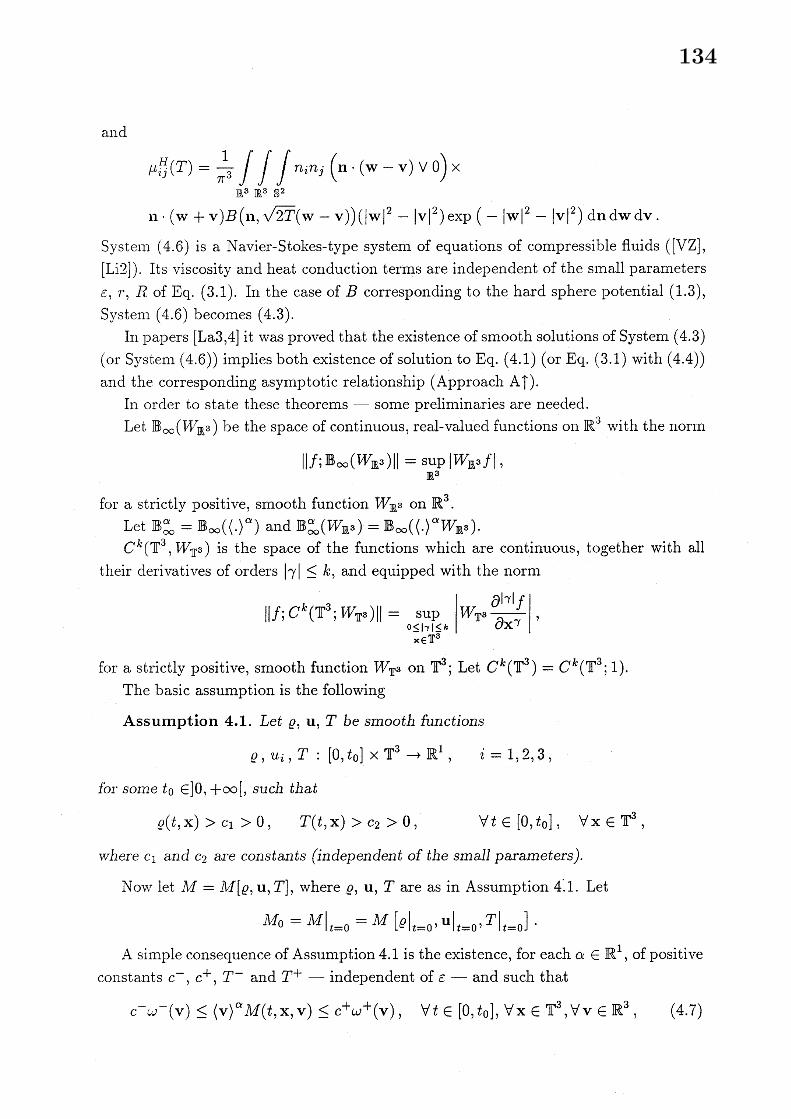
$\mu_{ij}^{H}(T)=\frac{1}{\pi^{3}}\int_{\mathrm{J}\mathrm{R}^{3}\mathrm{J}}\int_{\mathrm{R}^{3}\mathrm{S}}\int_{2}n_{i}n_{j}(\mathrm{n}\cdot(\mathrm{w}-\mathrm{v})\vee 0)\mathrm{x}$
$\mathrm{n}\cdot(\mathrm{w}+\mathrm{v})B(\mathrm{n}, \sqrt{2T}(\mathrm{w}-\mathrm{v}))(|\mathrm{w}|^{2}-|\mathrm{v}|^{2})\exp(-|\mathrm{w}|^{2}-|\mathrm{v}|^{2})$ dn dw $\mathrm{d}\mathrm{v}$ .
System (4.6) is a Navier-Stokes-type system of equations of compressible fluids ([VZ],[Li2] $)$ . Its viscosity and heat conduction terms are independent of the small parameters
$\epsilon,$ $r,$ $R$ of Eq. (3.1). In the case of $B$ corresponding to the hard sphere potential (1.3),Systee (4.6) becomes (4.3).
In papers [La3,4] it was proved that the existence of smooth solutions of System (4.3)(or System (4.6)) implies both existence of solution to Eq. (4.1) (or Eq. (3.1) with (4.4))and the corresponding asymptotic relationship (Approach $\mathrm{A}\uparrow$ ).
In order to state these theorems –some preliminaries are needed.Let $\mathrm{B}_{\infty}(\nu V_{\mathrm{R}^{3}})$ be the space of continuous, real-valued functions on $\mathbb{R}^{3}$ with the norm
$||f; \mathrm{B}_{\infty}(W_{\mathrm{R}^{3}})||=\sup_{\mathrm{R}^{3}}|W_{\mathrm{R}^{3}}f|$,
for a strictly positive, smooth function $W_{\mathrm{R}^{3}}$ on $\mathbb{R}^{3}$ .Let $\mathrm{B}_{\infty}^{\alpha}=\mathrm{B}_{\infty}(\langle.\rangle^{\alpha})$ and $\mathrm{B}_{\infty}^{\alpha}(W_{\mathrm{R}^{3}})=\mathrm{B}_{\infty}(\langle.\rangle^{\alpha}W_{\mathrm{R}^{3}})$.$C^{k}(\mathbb{T}^{3}, \nu V_{?\mathrm{I}^{3}},)$ is the space of the functions which are continuous, together with all
their derivatives of orders $|\gamma|\leq k$ , and equipped with the norm
$||f;C^{k}( \mathbb{T}^{3} ; W_{\mathrm{T}^{3}})||=0\leq|\gamma|\leq k\sup_{\mathrm{x}\in \mathrm{T}^{3}}|W_{\mathrm{T}^{3}}\frac{\partial^{|\gamma|}f}{\partial \mathrm{x}^{\gamma}}|$ ,
for a strictly positive, smooth function $W_{\mathrm{J}\mathrm{f}^{3}}$ on $\mathbb{T}^{3}$ ; Let $C^{k}(\mathbb{T}^{3})=C^{k}(\mathbb{T}^{3}$ ; 1 $)$ .The basic assumption is the following
Assumption 4.1. Let $\rho,$ $\mathrm{u},$$T$ be smooih function$s$
$\rho,$ $u_{i},$$T$ : $[0, t_{0}]\mathrm{x}\mathbb{T}^{3}arrow \mathbb{R}^{1}$ , $i=1,2,3$ ,
$\mathrm{f}ol$ . some $t_{0}\in$ ] $0,$ $+\infty$ [, such that
$\rho(t, \mathrm{x})>c_{1}>0$ , $T(t, \mathrm{x})>c_{2}>0$ , $\forall t\in[0, t_{0}]$ , $\forall \mathrm{x}\in \mathbb{T}^{3}$ ,
where $c_{1}$ alld $c_{2}$ are constants (independent of the small parameiers).
Now let $M=\mathrm{J}I[\rho, \mathrm{u}, T]$ , where $\rho,$ $\mathrm{u},$$T$ are as in Assumption 4.1. Let
$M_{0}=M|_{t=0}=M[\rho|_{t=0}, \mathrm{u}|_{t=0}, T|_{t=0}]$ .
A simple consequence of Assumption 4.1 is the existence, for each $\alpha\in \mathbb{R}^{1}$ , of positiveconstants $c^{-},$ $c^{+},$ $T^{-}$ and $T^{+}$ –independent of $\epsilon$ –and such that
$c^{-}\omega^{-}(\mathrm{v})\leq\langle \mathrm{v}\rangle^{\alpha}M(t,\mathrm{x},\mathrm{v})\leq c^{+}\omega^{+}(\mathrm{v})$ , $\forall t\in[0, t_{0}],$ $\forall \mathrm{x}\in \mathbb{T}^{3},\forall \mathrm{v}\in \mathbb{R}^{3}$ , (4.7)
134
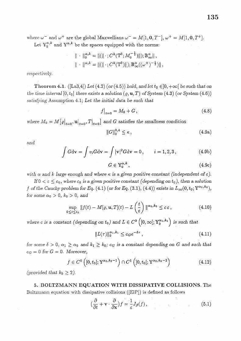
where $\omega^{-}$ and $\omega^{+}$ are the global Maxwellians $\omega^{-}=M[1,0, T^{-}],$ $\omega^{+}=M[1,0, T^{+}]$ .Let $\mathrm{Y}_{0}^{\alpha,k}$ and $\mathrm{Y}^{\alpha,k}$ be the spaces equipped with the norms:
$||$$||_{0}^{\alpha,k}=||(||\cdot ; C^{k}(\mathbb{T}^{3} ; M_{0}^{-\frac{1}{2}})||);\mathrm{B}_{\infty}^{\alpha}||_{y}$
$||$$||^{\alpha,k}=||(||\cdot ; C^{k}(\mathbb{T}^{3})||);\mathrm{B}_{\infty}^{\alpha}((\omega^{+})^{-\frac{1}{2}})||$ ,
respectively.
Theorem 4.1. $([\mathrm{L}\mathrm{a}3,4])$ Let (4.2) (or (4.5)) hold, and let $t_{0}\in$ ] $0,$ $+\infty[\mathrm{b}e$ such thai onthe $ti\mathrm{m}e$ interval $[0, t_{0}]$ ihere exists a $sol\mathrm{u}$ tion $(\rho, \mathrm{u}, T)$ of System (4.3) (or System (4.6))sa $tis\mathrm{f}\dot{y}i\mathrm{n}\mathrm{g}$ Assumption 4.1; Let the iniiial data be such that
$f|_{t=0}=M_{0}+G$ , (4.8)
nhere $M_{0}=M[\rho|_{t=0}, \mathrm{u}|_{t=0}, T|_{t=0}]$ and $G$ satisfies the smalln$ess$ condition
$||G||_{0}^{0,4}\leq\kappa$ , (4.9a)
an $d$
$\int G\mathrm{d}\mathrm{v}=\int v_{i}G\mathrm{d}\mathrm{v}=\int|\mathrm{v}|^{2}G\mathrm{d}\mathrm{v}=0$ , $i=1,2,3$ , (4.9b)
$G\in \mathrm{Y}_{0}^{\alpha,k}$ , (4.9c)$17^{f}ithc\mathrm{t}’$ and $k$ large $e\mathrm{J}\mathrm{z}\mathrm{o}\mathrm{u}\mathrm{g}h$ and wbere $\kappa$ is a given posiii $\iota^{\gamma}e$ constant (independent of $\epsilon$).
$I\mathrm{f}0<\epsilon\leq\epsilon_{0}$ , where $\epsilon_{0}$ is a given positive constant (depending on $t_{0}$ ), then a solution$f$ of the $C\mathrm{a}$uchy problem for Eq. (4.1) (or for Eq. (3.1), (4.4)) exists in $L_{\infty}(\mathrm{O}, t_{0}; \mathrm{Y}^{\alpha_{0},k_{0}})$ ,$\mathrm{f}\dot{c})\mathrm{r}$ some $\alpha_{0}>0,$ $k_{0}>0$ , and
$0 \leq t\leq t_{0}\mathrm{s}\mathrm{u}\mathrm{p}||f(t)-M[\rho, \mathrm{u}, T](t)-L(\frac{t}{\epsilon})||^{\alpha_{0},k_{0}}\leq c\epsilon$ , (4.10)
$n^{\gamma}herec$ is a constant (depending on $t_{0}$ ) and $L\in C^{0}([0, \infty[;\mathrm{Y}_{0}^{\alpha_{1},k_{1}})$ is such th$\mathrm{a}i$
$||L(\tau)||_{0}^{\alpha_{1},k_{1}}\leq cce^{-\delta\tau}$ , (4.11)
$\mathrm{f}ol$ ’ some $S>0,$ $\alpha_{1}\geq\alpha_{0}$ and $k_{1}\geq k_{0}$ ; $C_{G}$ is a constant depending on $G$ and such that$cc=0\mathrm{f}ol\cdot G=0$ . Moreover,
$f\in C^{0}([0,t_{0}];\mathrm{Y}^{\alpha_{0},k_{0}-1})\cap C^{1}(]0,t_{0}$ [; $\mathrm{Y}^{\alpha_{0)}k_{0}-2})$ (4.12)
(provided $tl_{2}\mathrm{a}tk_{0}\geq 2$).
5. BOLTZMANN EQUATION WITH DISSIPATIVE COLLISIONS. The$\mathrm{B}\mathrm{o}\mathrm{l}\mathrm{t}\mathrm{z}\mathrm{n}\grave{\perp}\mathrm{a}\mathrm{n}\mathrm{n}$ equation with dissipative collisions $([\mathrm{E}\mathrm{l}\mathrm{P}])$ is defined as follows
$( \frac{\partial}{\partial t}+\mathrm{v}\cdot\frac{\partial}{\partial \mathrm{x}})f=\frac{1}{\epsilon}J_{\beta}(f^{\backslash })$ , (5.1)
135

where$J_{\beta}(f)(\mathrm{x}, \mathrm{v})=$
$\int_{\mathrm{J}\mathrm{R}^{3}\mathrm{S}}\int_{2}(\frac{1}{(2\beta-1)^{2}}f(\mathrm{x},\hat{\mathrm{w}})f(\mathrm{x},\hat{\mathrm{v}})-f(\mathrm{x}, \mathrm{v})f(t,\mathrm{x}, \mathrm{w}))(\mathrm{n}\cdot(\mathrm{w}-\mathrm{v})\vee 0)$
dn $\mathrm{d}\mathrm{w}$ ,
$\hat{\mathrm{v}}=\mathrm{v}+\frac{1-\beta}{1-2\beta}\mathrm{n}\cdot(\mathrm{w}-\mathrm{v})$ , $\hat{\mathrm{w}}=\mathrm{w}-\frac{1-\beta}{1-2\beta}\mathrm{n}\cdot(\mathrm{w}-\mathrm{v})$ , (5.2)
are the velocities before a collision which produce the velocities $\mathrm{v},$$\mathrm{w}$ , respectively, after
the collision, $\beta\in$ ] $0,$ $\frac{1}{2}$ [is a dimensionless parameter characterizing energy dissipation.
The unique solution to the degenerate equation (for $\beta>0$ –fixed)
$J_{\beta}(f)=0$ (5.3)
is the trivial one $f\equiv 0-\mathrm{s}\mathrm{e}\mathrm{e}$ [BEL].
Under the assumption
$\beta=b\epsilon$ , $b=\mathrm{c}\mathrm{o}\mathrm{n}\mathrm{s}\mathrm{t}$ , (5.4)
Equation (5.1) formally results (cf. [BEL]) in the following Euler system
$\frac{\partial\rho}{\partial t}+\sum_{i=1}^{3}\frac{\partial}{\partial x_{i}}(\rho u_{i})=0$ , (5.5a)
$\rho\frac{\partial u_{j}}{\partial t}+\rho\sum_{i=1}^{3}u_{i}\frac{\partial u_{j}}{\partial x_{i}}+\frac{\partial}{\partial x_{j}}(\rho T)=0$ , $j=1,2,3$ , (5.5b)
$\frac{\partial T}{\partial t}+\sum_{i=1}^{3}u_{i}\frac{\partial T}{\partial x_{i}}+\frac{2}{3}T\sum_{i=1}^{3}\frac{\partial u_{i}}{\partial x_{i}}=-c_{0}b\rho T^{3/2}$ , (5.5c)
where $c_{0}$ is a given positive constant.
6. UEHLING-UHLENBECK QUANTUM EQUATION. The Uehling-Uh-
lenbeck equation ([UU], [CC], [KB] and [Su], [Do], [Lil]), describing the evolution of a
gas of quantum particles, is defined as follows
$( \frac{\partial}{\partial t}+\mathrm{v}\cdot\frac{\partial}{\partial \mathrm{x}})f=\frac{1}{\epsilon}\mathfrak{Q}_{\frac{\lambda}{\epsilon}}(f)$ , (6.1)
$\mathfrak{Q}_{\frac{\lambda}{\epsilon}}(f)(\mathrm{x}, \mathrm{v})=\int_{\mathrm{J}\mathrm{R}^{3}\mathrm{S}}\int_{2}(f(\mathrm{x},\mathrm{v}’)f(\mathrm{x},\mathrm{w}’)(1-\frac{\lambda}{\epsilon}f(\mathrm{x}, \mathrm{v}))(1-\frac{\lambda}{\epsilon}f(\mathrm{x}, \mathrm{w}))-$
$f( \mathrm{x}, \mathrm{v})f(\mathrm{x}, \mathrm{w})(1-\frac{\lambda}{\epsilon}f(\mathrm{x}, \mathrm{v}’))(1-\frac{\lambda}{\epsilon}f(\mathrm{x},\mathrm{w}’)))B(\mathrm{w}-\mathrm{v}, \mathrm{n})\mathrm{d}\mathrm{n}\mathrm{d}\mathrm{w}$;
$/\backslash \mathrm{i}\mathrm{s}$ a parameter (proportional to $h^{3}$ ), that is$(+)$ positive for fermions and
136

(–) negative for bosons.
One can expect that the class of solutions of the degenerate equation correspondingto the singularly perturbed equation (6.1), for $\epsilonarrow 0$ and fixed $\lambda>0$ , is too small to
describe a reasonable hydrodynamic. Therefore the following limit
$\epsilon\downarrow 0$ , $\lambda\downarrow 0$ , (6.2)
should be considered.
One can distinguish the following important cases$(\mathrm{i}.)|\lambda|\ll\epsilon$ , (e.g. $|\lambda|=\epsilon^{p}$ for $p>1$ ) –it can be treated in the same way as the
$\mathrm{c}\mathrm{o}\mathrm{l}\cdot \mathrm{r}\mathrm{e}\mathrm{s}\mathrm{p}\mathrm{o}\mathrm{n}\mathrm{d}\mathrm{i}\mathrm{n}\mathrm{g}$ problem for the classical Boltzmann equation;$(\mathrm{i}\mathrm{i}.)|\lambda|\gg\epsilon$ , (e.g. $|\lambda|=\epsilon^{p}$ for $p<1$ ) $-\mathrm{i}\mathrm{t}$ is not physically consistent;
$(\mathrm{i}\mathrm{i}\mathrm{i}.)|/\backslash |\sim\in,$ (e.g. $|/\backslash |=\epsilon$ ).$\mathrm{C}^{1}\mathrm{o}\mathrm{n}\mathrm{s}\mathrm{i}\mathrm{d}\mathrm{e}\mathrm{r}$ the two cases
$\lambda=\epsilon$ (6.3a)
–fermions –the $\mathrm{s}\mathrm{u}\mathrm{b}\mathrm{s}\mathrm{c}\mathrm{r}\mathrm{i}\mathrm{p}\mathrm{t}+\mathrm{i}\mathrm{s}$ used, e.g. $\mathfrak{Q}_{+}=\mathfrak{Q}_{+1}$ , and
$/\backslash =-\mathcal{E}$ (6.3b)
–bosons –the subscript–is used, e.g. $\mathfrak{Q}_{-}=\mathrm{i}\supset_{-1}$ .Solutions to the degenerate equations
$\mathfrak{Q}_{\pm}(f)=0$ (6.4)
are given by
$S \pm(t, x, v)=\frac{M(t,x,v)}{1\pm M(t,x,v)}$ , (6.5)
where $\wedge \mathrm{t}/[=\mathit{1}\backslash p_{\pm}[\gamma, \mathrm{u}, \tau]$ are Maxwellians with fluid-dynamic parameters $\gamma=\gamma\pm,$ $\mathrm{u}=$
$\mathrm{u}_{\pm},$ $\tau=\mathcal{T}\pm;s_{+}$ is called the Fermi-Dirac distribution, whereas $s_{-}-$ the Bose-Einstein
distribution.
The fluid dynamic parameters $\rho\pm,$ $\mathrm{u}\pm,$$\mathrm{t}\pm \mathrm{o}\mathrm{f}\mathfrak{F}\pm \mathrm{a}\mathrm{r}\mathrm{e}$ related to the fluid-dynamic
parameters $\gamma\pm,$$u\pm \mathrm{a}\mathrm{n}\mathrm{d}_{\mathcal{T}\pm}$ of the corresponding Maxwellians by some given functions
(see (2.10) in [AL2]).
Forlnally, in Cases (6.3), Eqs. (5.1) results in the classical Euler system at the O-th$\mathrm{O}1^{\backslash }\mathrm{d}\mathrm{e}1^{\cdot}$ of approximation ([AL1]) and in the following Navier-Stokes system at the l-st
order of approximation $([\mathrm{L}\mathrm{a}2])$
$\frac{\partial\rho}{\partial t}+\sum_{i=1}^{3}\frac{\partial}{\partial x_{i}}(\rho u_{i})=0$ , (6.6a)
137

$\rho\frac{\partial u_{j}}{\partial t}+\rho\sum_{i=1}^{3}u_{i}\frac{\partial u_{j}}{\partial x_{i}}+\frac{2}{3}\frac{\partial}{\partial x_{j}}(\rho \mathfrak{e})=\epsilon(\sum_{i=1}^{3}\frac{\partial}{\partial x_{i}}(\mu_{\pm}(\rho, \mathfrak{e})(\frac{\partial u_{j}}{\partial x_{i}}+\frac{\partial u_{i}}{\partial x_{j}}))-$
$\frac{2}{3}\frac{\partial}{\partial x_{j}}(\mu\pm(\rho, \mathfrak{e})\sum_{i=1}^{3}\frac{\partial u_{i}}{\partial x_{i}}))$ , $j=1,2,3$ ,
(6.6b)
$\frac{\partial \mathfrak{e}}{\partial t}+\sum_{i=1}^{3}u_{i}\frac{\partial \mathfrak{e}}{\partial x_{i}}+\frac{2}{3}\mathrm{e}\sum_{i=1}^{3}\frac{\partial u_{i}}{\partial x_{i}}=\frac{\epsilon}{\mathcal{G}\pm(\rho,\mathfrak{e})}(\sum_{i=1}^{3}\frac{\partial}{\partial x_{i}}(\mu_{\pm}^{(1)}(\rho, \mathfrak{e})\frac{\partial \mathrm{e}}{\partial x_{i}}+\mu_{\pm}^{(2)}(\rho, \mathfrak{e})\frac{\partial\rho}{\partial x_{i}})+$
$\mu_{\pm}(\rho, \mathfrak{e})\sum_{i,k=1}^{3}\frac{\partial u_{k}}{\partial x_{i}}(\frac{\partial u_{k}}{\partial x_{i}}+\frac{\partial u_{i}}{\partial x_{k}})-\frac{2}{3}\mu\pm(\rho, \mathfrak{e})(\sum_{i=1}^{3}\frac{\partial u_{i}}{\partial x_{i}})^{2})$ , (6.6c)
where $\mu_{\pm}(\rho, \mathrm{e}),$ $\mathcal{G}\pm(\rho, \mathfrak{e}),$$\mu_{\pm}^{(1)}(\rho, \mathfrak{e}),$ $\mu_{\pm}^{(2)}(\rho, \mathfrak{e})$ are given functions (cf. [AL2]) depending
on $B$ .
In papers [AL1,2] it was proved that the existence of smooth solutions of the Eulersystem or of System (6.6) implies both existence of solution to the kinetic equations (6.1)
and the corresponding asymptotic relationships (Approach $\mathrm{A}\uparrow$ ).
The results were obtained under the assumption that the solution $(\rho, \mathrm{u}, \mathfrak{e})$ to thehydrodynamic system satisfies the following inequality
$\mathfrak{e}>l_{\pm\rho^{\frac{2}{3}}}$ , (6.7)
for every $(t, \mathrm{x})\in[0, t_{0}]\cross \mathbb{T}^{3}$ , where $\iota_{+}$ and $l$-are given positive constants, respectively,for fermions $(+)$ and for bosons (-). Inequalities (6.7) are essential for the asymptoticrelationships (see [AL2]). In fact, under Conditions (6.7) the correspondence between$(\gamma\pm, \mathrm{u}\pm, \tau\pm)$ and the fluid-dynamic parameters $(\rho\pm, \mathrm{u}_{\pm}, \mathfrak{e}_{\pm})$ of $\mathrm{f}\mathrm{f}\pm \mathrm{i}\mathrm{s}\mathrm{o}\mathrm{n}\mathrm{e}-\mathrm{t}\mathrm{o}-\mathrm{o}\mathrm{n}\mathrm{e}$, re-spectively $\mathrm{f}\mathrm{o}\mathrm{r}+\mathrm{a}\mathrm{n}\mathrm{d}-$ .
In order to state the theorems from [AL2] –some preliminaries are needed.Assumption 6.1. Let $\gamma\pm,$ $\mathrm{u}_{\pm}$ and $\tau\pm \mathrm{b}e$ smooth functions
$\gamma\pm,$ $u_{i\pm},$$\mathcal{T}\pm:[0, t_{0}]\cross \mathbb{T}^{3}arrow \mathbb{R}^{1}$ , $i=1,2,3$ ,
for some $t_{0}\in$ ] $0,$ $+\infty$ [, such that
$\wedge(\pm(t, \mathrm{x})>c_{1}>0,$ $\mathcal{T}\pm(t, \mathrm{x})>c_{2}>0$ , $\forall t\in[0, t_{0}]$ , $\forall \mathrm{x}\in \mathbb{T}^{3}$ , (6.8)
wbere $c_{1}$ and $c_{2}$ are consiants. Moreo$\mathrm{v}er$ let
$\gamma_{-}(t, \mathrm{x})\leq\delta<1$ , $\forall t\in[0, t_{0}]$ , $\forall \mathrm{x}\in \mathbb{T}^{3}$ (6.9)
Consider Maxwellians with parameters $\gamma\pm,$ $\mathrm{u}_{\pm},$$\mathcal{T}\pm \mathrm{s}\mathrm{a}\mathrm{t}\mathrm{i}\mathrm{s}\mathrm{f}\mathrm{y}\mathrm{i}\mathrm{n}\mathrm{g}$ Assumption 6.1 and
let {$\zeta_{\pm}$ be defined by Eqs. (6.5).
138

A simple consequence of Assumption 6.1 is the existence, for each $\alpha\in \mathbb{R}^{1}$ , of positiveconstants $c_{\pm}^{-},$
$c_{\pm}^{+},$$\tau_{\pm}^{-},$ $\tau_{\pm}^{+}-$ independent of $\epsilon$ –and such that
$c_{\pm}^{-}\omega_{\pm}^{-}(\mathrm{v})\leq\langle \mathrm{v}\rangle^{\alpha}S\pm(t, \mathrm{x}, \mathrm{v})\leq c_{\pm}^{+}\omega_{\pm}^{+}(\mathrm{v})$ $\forall t\in[0, t_{0}],$$\forall \mathrm{x}\in \mathbb{T}^{3}$ , $\forall \mathrm{v}\in \mathbb{R}^{3}$ , (6.10)
where $\omega_{\pm}^{-}$ and $\omega_{\pm}^{+}$ are the global Maxwellians $\omega_{\pm}^{-}=M[1,0, \tau_{\pm}^{-}],$ $\omega_{\pm}^{+}=M[1,0, \tau_{\pm}^{+}]$ .Let $\mathrm{Y}_{\pm}^{\alpha,k}$ and $||\cdot||_{\pm}^{\alpha,k}$ be defined as $\mathrm{Y}^{\alpha,k}$ and $||\cdot||^{\alpha_{)}k}$ in Section 4, but with $\omega_{\pm}^{+}$ instead
of $\omega^{+}$ .The results of [AL2] both for the classical Euler system and for the Navier-Stokes
system (6.6) as well as both for fermions and for bosons can be summarized as follows
Theorem 6.1. Let either of $Co\mathrm{n}$ ditions (6.3) hold and let $t_{0}\in$ ] $0,$ $\infty$ [ be independentof $\epsilon$ such that on the iime $\mathrm{i}nter\iota^{\gamma}al[0, t_{0}]$ there exisis a smooth solution $(\rho\pm, \mathrm{u}\pm, \mathfrak{e}\pm)$ ofthe Navier-Stokes system (6.6) (or the classical Euler sysiem) that saiisfies (6.7) andcorresponds to $p$arameters $(\gamma\pm, \mathrm{u}_{\pm,\pm}\tau)$ satisfying Assumpiion 6.1 togeiher wiih theconditions of uniformly boundedness with respect to $\epsilon$ of the quantities
$\sup$ $\gamma\pm$ , $\sup$ $|\mathrm{u}_{\pm}|$ , $\sup$ $\mathcal{T}\pm$ ;$[0,t_{0}]\cross \mathrm{T}^{3}$ $[0,t_{0}]\cross \mathbb{T}^{3}$ $[0,t_{0}]\cross \mathrm{T}^{3}$
Let the initi $\mathrm{a}l$ daia be either of the functions (6.5) with parameiers $\gamma\pm|_{t=0},$ $\mathrm{u}_{\pm}|_{t=0}$ ,$\mathcal{T}\pm|_{t=0}$ corresponding to $\rho\pm|_{t=0},$ $\mathrm{u}_{\pm}|_{t=0},$ $\mathfrak{e}\pm|_{t=0}$ .
If $0<\epsilon\leq\epsilon_{0}$ , where $\epsilon_{0}$ is a given posi $ti\mathrm{v}e$ constant (depending on $t_{0}$ ), then asoluiion $f$ of the CaucAy problem for Eq. (6.1) exists in $L_{\infty}(\mathrm{O}, t_{0} ; \mathrm{Y}_{\pm}^{\alpha,k})$ , for some $\alpha>0$ ,$k>0$ , an $d$
$f\in C^{0}([0, t_{0}];\mathrm{Y}_{\pm}^{\alpha,k-1})\cap C^{1}(]0,$ $t_{0}$ [; $\mathrm{Y}_{\pm}^{\alpha,k-2})$ (if $k\geq 2$), (6.10)
$[] \sup_{0,t_{0}}||f-\mathfrak{F}\pm||_{\pm}^{\alpha,k}\leq c\epsilon$ , (6.11)
$wl2ereS\pm is$ deffied by parameters $(\gamma\pm, \mathrm{u}_{\pm}, \tau_{\pm})$ corresponding to $(\rho\pm, \mathrm{u}_{\pm}, \mathfrak{e}_{\pm})$ and $c$
$is$ a positi $\iota^{\gamma}e$ consiant (depending on $t_{0}$ ).
An analogous theorem can be obtained for more general data if one includes initiallayer as in Theorem (4.1).
139
References
[Arl] Arkeryd L., On the Enskog equation in two space variables, Transport Theory Statist. Phys., 15, 1986, 673-691.
[Ar2] Arkeryd L., On the Enskog equation with large data, SIAM J. Math. Anal., 21, 1990, 631-646.
[AC1] Arkeryd L., &Cercignani C., On the convergence of solutions of the Enskog equation to solutions of the Boltzmann
equation, Comm. Part. Diff. Eq., 14, 1989, 1071–1089.
$[\mathrm{A}\mathrm{C}^{}2]\mathrm{A}\mathrm{r}\mathrm{k}\mathrm{e}\mathrm{l}\cdot \mathrm{y}\mathrm{d}$ L., &Cercignani C., Global existence in $L^{1}$ for the Enskog equation and convergence of the solutions to
solutions of the Boltzmann equation, J. Statist. Phys., 59, 1990, 3-4, 845-867.
[AL1] Arlotti L., &Lachowicz M., On the hydrodynamic limit for quantum kinetic equations, Compt. Rend. Acad. Sci.
Paris 323, S\’erie I, 1996, 101-106.
[AL2] Arlotti L., &Lachowicz M., Euler and Navier-Stokes hmits of the Uehling-Uhlenbeck quantum kinetic equations, J.
Math. Phys., 38, 1997, 3571-3588.
[Anl] Arsen’ev A.A., The Cauchy problem for the linearized Boltzmann equation, Zh. Vychisl. Mat. $\mathrm{i}$ Mat. Fiz., 5, 1965,
864-882, in Russian.
[An2] Arsen’ev A.A., Approximation of the Boltzmann equation by stochastic equations, Zh. Vychisl. Mat. $\mathrm{i}$ Mat. Fiz., 28,
1988, 560-567, in Russian.
[An3] Arsen’ev A.A., Lectures on kinetic equations, Nauka, Moscow 1992, in Russian.
[At] Arlotti L., On a functional equation in mathematical kinetic theory, Transport Theory Statist. Phys., 26, 6, 1997,
639-660.
[AU] Asano $l<.$ , &Ukai S., On the fluid dynamical limit of the Boltzmann equation, in Lecture Note in Numer. Appl. Anal.,
Recent Topics in Nonlinear PDE, 6, Eds. Mimura M., &Nishida T., $\mathrm{N}\mathrm{o}\mathrm{r}\mathrm{t}\mathrm{h}-\mathrm{H}\mathrm{o}\mathrm{U}\mathrm{a}\mathrm{n}\mathrm{d}$ and Kinokuniya 1984, 1-20.
[BLPT] Bellomo N., Lachowicz M., Polewczak J., &Toscani G., Mathematical Topics in Nonlinear Kinetic Theory II: The
Enskog Equation, World Sci., Singapore 1991.
[BEL] Bellomo N., Esteban M., &Lachowicz M., Nonlinear kinetic equations with dissipative collisions, Appl. Math. Lett.,
8, 5, 1995, 47-52.
[ $\mathrm{B}\mathrm{G}$‘Ll] Bardos C., Golse F., &Levermore D., Sur les limites asymptotiques de la th\’eorie cin\’etique $\mathrm{c}\mathrm{o}\mathrm{n}\mathrm{d}\iota\dot{\mathrm{u}}\mathrm{s}\mathrm{a}\mathrm{n}\mathrm{t}$ \‘a la dinamique
des fluides incompressibles, Comp. Rend. Acad. Sci. Paris, 309, Serie I, 1989, 727-732.
[BGL2] Bardos C., Golse F., &Levermore D., Fluid dynanics hmits of kinetic equations I: Formal derivation, J. Statist. Phys.,
63, 1991, 323-344.
[BGL3] Bardos C., Golse F. &Levermore D., Fluid dynamics limits of kinetic equations II, Comm. Pure Appl. Math., 46,
1993, 667-753.
[BP] Bellomo N., &Polewczak J., The generalized Boltzmann equation, solution and exponential trend to equihbrium,
Transport Theory Statist. Phys., 26, 6, 1997, 661-677.
[BU] Bardos C., &Ukai S., The classical incompressible Navier-Stokes limit of the boltzmann equation, Math. Models
Meth. Appl. Sci., 1, 2, 1991, 135-257.
[Cal] Caflisch R., The fluid dynamic limit of the nonlinear Boltzmann equation, Comm. Pure $\mathrm{A}_{\mathrm{P}1)}1$ . Math., 33, 1980,
651-666.
[Ca2] Cafhsch R., Asymptotic expansions of solutions for the Boltzmann equation, Transport Theory Statist. Phys., 16, 4-6,
1987, 701-725.
140
[CC] Chapman S., &Cowling T.G., The Mathematical Theory of $\mathrm{N}\mathrm{o}\mathrm{n}\mathrm{u}\iota\dot{\mathrm{u}}\mathrm{f}\mathrm{o}\mathrm{r}\mathrm{m}$ Gases, Cambridge Univ. Press, Cambridge
1970.
[Cel] Cercignani C., The $\mathrm{G}\mathrm{r}\mathrm{a}\mathrm{d}$ limit for a system of soft spheres, Comm. Pure Appl. Math., 36, 1983, 479-494.
[Ce2] $\mathrm{C}\mathrm{e}\mathrm{l}\cdot \mathrm{c}\mathrm{i}\mathrm{g}\mathrm{n}\mathrm{a}\mathrm{n}\mathrm{i}$ C., Existence of global solutions for the space iffiomogeneous Enskog equation, Transport Theory Statist.
Phys., 16, 1987, 213-221.
[CIP] Cercignani C., Illner R., &Pulvirenti M., The Mathematical Theory of Dilute Gases, Springer, New York 1994.
[DL] $\mathrm{D}\mathrm{i}\mathrm{P}\mathrm{e}\mathrm{r}\mathrm{n}\mathrm{a}$ R., &Lions P.L., On the Cauchy problem for the Boltzmann equation: Global existence and weak stability
results, Ann. Math., 130, 1990, 1189-1214.
[DEL] $\mathrm{D}\mathrm{e}\mathrm{M}\mathrm{a}\mathrm{s}\mathrm{i}$ A., Esposito R., &Lebowitz J.L., Incompressible Navier-Stokes and Euler limits of the Boltzmann equation,
Comm. Pure Appl. Math., 42, 1989, 1189-1214.
[Do] Dolbeault J., $\mathrm{I}<\mathrm{i}\mathrm{n}\mathrm{e}\mathrm{t}\mathrm{i}\mathrm{c}$ models and quantum effects: A modified Boltzmann equation for Fermi-Dirac particles, Arch.
Rational Mech. Anal., 127, 1994, 101-131.
$[\mathrm{E}\mathrm{l}\mathrm{P}]$ Ellis R.S., &\acute Pinsky M.A., The $\mathrm{f}\mathrm{i}_{1}\cdot \mathrm{s}\mathrm{t}$ and second fluid approximations to the linearized Boltzmann equation, J. Math.
Pure Appl., 54, 1975, 125-156.
$[1^{-}_{\lrcorner}\mathrm{s}\mathrm{P}]$ Es $\mathrm{f}$ eball $1\backslash q.$ , &Perthame $\mathrm{B}_{)}$. On the modified Enskog equation for elastic and inelastic collisions. Models with spin,
Ann. Inst. H. Poincar\’e--Anal. Non Lin\’eaire, 8, 1991, 289-308.
[FE] Felziger $\mathrm{J}.\mathrm{H}.$ , &Kaper H.G., Mathematical Theory of Transport Processes in Gases, $\mathrm{N}\mathrm{o}\mathrm{r}\mathrm{t}\mathrm{h}-\mathrm{H}\mathrm{o}\mathrm{U}\mathrm{a}\mathrm{n}\mathrm{d}$ 1972.
[Go] Golce F., Incompressible hydrodynamic as a limit of the Boltzmann equation, Transport Theory Statist. Phys., 21,
1992, 531-555.
[Gr] $\mathrm{G}\mathrm{r}\mathrm{a}\mathrm{d}$ H., Asymptotic theory of the Boltzmann equation. II, in Rarefied Gas Dynamics, vol. I, Ed. Laurmann J.,
Academic Press 1963, 26-59.
[TL] $\mathrm{J}\mathrm{a}\mathrm{g}\mathrm{o}\mathrm{d}\mathrm{z}\mathrm{i}1’1\mathrm{s}\mathrm{k}\mathrm{i}$ S.. &Lachowicz M., Incolnpressible Navier-Stokes limit for the Enskog equation, Appl. Math. Letters. to
appear.
[IGB] Kadanoff L.P., &Baym G., Quantum Statistical Mechanics, Addison-Wesley Pub. Co., Redwood City 1989.
$[\mathrm{I}<\mathrm{M}\mathrm{N}]\mathrm{I}<\mathrm{a}\backslash \backslash ’ \mathrm{a}\mathrm{s}\mathrm{h}\mathrm{i}\mathrm{m}\mathrm{a}$ S., Matsumura A., &Nishida T., On the fluid-dynamical approximation to the Boltzmann equation at
the level of the Navier-Stokes equation, Commun. Math. Phys., 70, 1979, 97–124.
$[1_{}\mathrm{a}1]\mathrm{L}\mathrm{a}\mathrm{d}_{1}\mathrm{o}\mathrm{w}\mathrm{i}\mathrm{c}\mathrm{z}$ M., A system of stochastic differential equations modeling the Euler and the Naviel-Stokes hydrodynamic
equctions, $\mathrm{J}\mathrm{a}_{1^{J\mathrm{a}\mathrm{n}}}$ J. Industr. Appl. Math., 10, 1993, 109-131.
$[1_{\lrcorner}\mathrm{a}2]\mathrm{L}\mathrm{a}\mathrm{t}_{J}1\mathrm{t}\mathrm{o}\mathrm{w}\mathrm{i}\mathrm{c}\mathrm{z}$ M., Asymptotic analysis of nonlinear kinetic equations: The hydrodynamic limit, in Lecture Notes on the
Mathematical Theory of the Boltzmann equation, World Sci., Singapore 1995, 65-148.
[La3] Lachowicz M., From kinetic to $\mathrm{N}\mathrm{a}\mathrm{v}\mathrm{i}\mathrm{e}\mathrm{r}-\mathrm{S}\mathrm{t}\mathrm{o}\mathrm{k}\mathrm{e}\mathrm{s}$ -type equations, Appl. Math. Lett., 10, 5, 1997, 19-23.
[La4] $\mathrm{L}\mathrm{a}\mathrm{c}_{\vee}1_{1}\mathrm{o}\mathrm{w}\mathrm{i}\mathrm{c}\mathrm{z}$ M., Hydrodynamic limits of stochastic kinetic equations I, ARI, 50, 2, 1997, 131-140.
[La5] $\mathrm{L}\mathrm{a}\mathrm{c}\mathrm{l}\iota \mathrm{o}\mathrm{w}\mathrm{i}\mathrm{c}\mathrm{z}$ M., On the hydrodynamic limit of the Enskog equation, Publ. Res. Inst. Math. Sci., 34, 1998, 191-210.
[Lil] Lions P.-L., $\mathrm{C}\mathrm{o}\mathrm{I}\mathrm{n}\mathrm{p}\mathrm{a}\mathrm{c}\mathrm{t}\mathrm{n}\mathrm{e}\mathrm{s}\mathrm{s}$in Boltzmann’s equation via Fourier integral operators and applications. III, J. Math. Kyoto
Univ. 34, 3, 1994, 539-584.
[Li2] Lions P.-L., On some recent methods for nonlinear partial differential equations, in Proceedings of the International
$\mathrm{C}^{}\mathrm{o}\mathrm{n}\mathrm{g}\mathrm{r}\mathrm{e}\mathrm{s}\mathrm{s}$ of Mathematicians, Z\"urich 1994, Birkh\"auser Verlag 1994, 140-155.
[Le] Leray J.) Easai sur le mouvement d’un liquide visqueux emplissant l’espace, Acta Math., 63, 1934, 193-248.
141
[LP] Lachowicz M., &Pulvirenti M., A stochastic particle system modeling the Euler equation, $\mathrm{A}\mathrm{r}\mathrm{c}1_{1}$ . Rational Mech. Anal.,
109, 1, 1990, 81-93.
[Mo] Morgenstern D., Analytical studies related to the MaxweU-Boltzmann equation, Arch. Rational Mech. Anal., 4, 1955,
533-555.
[Ni] $\mathrm{N}\mathrm{i}\mathrm{s}\mathrm{l}\dot{\mathrm{u}}\mathrm{d}\mathrm{a}$ T., Fluid dynamical limit of the nonlinear Boltzmann equation to the level of the compressible Euler equation,
Conlm. Math. Phys., 61, 1978, 119-148.
[Po] Povzner A.Ya., The Boltzmann equation in the kinetic theory of gases, Amer. Math. Soc. Transl. (2), 47, 1962,
193-216.
[Pv] $\mathrm{V}.\mathrm{P}$ . Polityukov V.P., Solution of the Cauchy problem for the nonlinear Uehling-Uhlenbeck equation, Doklady Akad.
Nauk, 312, 6, 1990, 1357-1360, in Russian.
[Si] Sideris T., Formation of singularities in three dimensional compressible fluids, Comm. Math. Phys., 101, 1985, 475-485.
[Su] Suslin V.M., Existence theorems for kinetic equations with the Uehling-Uhlenbeck collision integral, Doklady Akad.
Nauk, 328, 5, 1993, 567-569, in Russian.
[Uk] Ukai S., Solutions of the Boltzmann equation, Patterns and Waves –Qualitative Analysis of Nonlinear Differential
Equations, 18, North-Holland and Kinokuniya, 1986, 18, 37-96.
[UA] Ukai S., &Asano K., The Euler limit and initial layer of the nonlinear Boltzmann equation, Hokkaido Math. J., 12,
$\mathrm{n}$ . $3$ , 1983, 311-332.
[UU] Uehling $\mathrm{E}$ A., &Uhlenbeck G.E., Transport phenomena in Einstein-Bose and Fermi-Dirac gases, Phys. Rev., 43, 1933,
552-561.
[Vo] Voronina V.A., A stochastic methods of solving an $\mathrm{i}\mathrm{n}\mathrm{i}\mathrm{t}\mathrm{i}\mathrm{a}\mathrm{l}- \mathrm{b}\mathrm{o}\iota \mathrm{m}\mathrm{d}\mathrm{a}\mathrm{r}\mathrm{y}$-value problem for the Boltzmann equation, Zh.
Vychisl. Mat. $\mathrm{i}$ Mat. Fiz., 32, 4, 1992, 576-586, in Russian.
[VZ] Valli A., &Zajaczkowski W., Navier-Stokes equations for compressible fluid: global existence and qualitative properties
of the solutions in the general case, Comm. Math. Phys., 103, 1986, 259-296.
142