equalities and inequalities : irreversibility and the second law of

Seminaire Poincare XV Le Temps (2010) 77 – 102 Seminaire Poincare

Equalities and Inequalities : Irreversibility and the Second Law ofThermodynamics at the Nanoscale

Christopher JarzynskiDepartment of Chemistry and Biochemistryand Institute for Physical Science and TechnologyUniversity of MarylandCollege Park MD 20742, USA

1 Introduction

On anyone’s list of the supreme achievements of the nineteenth-century science,both Maxwell’s equations and the second law of thermodynamics surely rank high.Yet while Maxwell’s equations are widely viewed as done, dusted, and uncontro-versial, the second law still provokes lively arguments, long after Carnot publishedhis Reflections on the Motive Power of Fire (1824) and Clausius articulated theincrease of entropy (1865). The puzzle at the core of the second law is this : how canmicroscopic equations of motion that are symmetric with respect to time-reversalgive rise to macroscopic behavior that clearly does not share this symmetry ? Ofcourse, quite apart from questions related to the origin of “time’s arrow”, there isa nuts-and-bolts aspect to the second law. Together with the first law, it provides aset of tools that are indispensable in practical applications ranging from the designof power plants and refrigeration systems to the analysis of chemical reactions.

The past few decades have seen growing interest in applying these laws andtools to individual microscopic systems, down to nanometer length scales. Muchof this interest arises at the intersection of biology, chemistry and physics, wherethere has been tremendous progress in uncovering the mechanochemical details ofbiomolecular processes. [1] For example, it is natural to think of the molecular com-plex φ29 – a motor protein that crams DNA into the empty shell of a virus – as ananoscale machine that generates torque by consuming free energy. [2] The deve-lopment of ever more sophisticated experimental tools to grab, pull, and otherwisebother individual molecules, and the widespread use of all-atom simulations to studythe dynamics and the thermodynamics of molecular systems, have also contributedto the growing interest in the “thermodynamics of small systems”, as the field issometimes called. [3]

Since the rigid, prohibitive character of the second law emerges from the sta-tistics of huge numbers, we might expect it to be enforced somewhat more lenientlyin systems with relatively few degrees of freedom. To illustrate this point, considerthe familiar gas-and-piston setup, in which the gas of N ∼ 1023 molecules beginsin a state of thermal equilibrium, inside a container enclosed by adiabatic walls. Ifthe piston is rapidly pushed into the gas and then pulled back to its initial location,there will be a net increase in the internal energy of the gas. That is,

W > 0, (1)

78 C. Jarzynski Seminaire Poincare

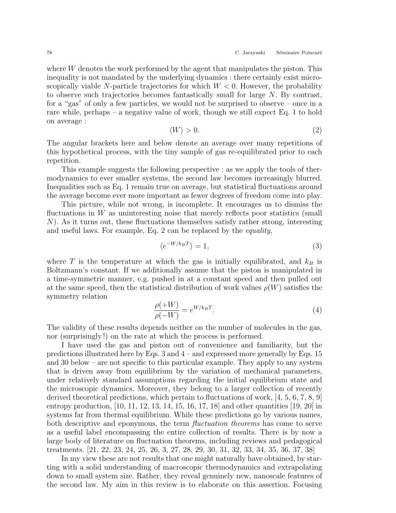
where W denotes the work performed by the agent that manipulates the piston. Thisinequality is not mandated by the underlying dynamics : there certainly exist micro-scopically viable N -particle trajectories for which W < 0. However, the probabilityto observe such trajectories becomes fantastically small for large N . By contrast,for a “gas” of only a few particles, we would not be surprised to observe – once in arare while, perhaps – a negative value of work, though we still expect Eq. 1 to holdon average :

〈W 〉 > 0. (2)

The angular brackets here and below denote an average over many repetitions ofthis hypothetical process, with the tiny sample of gas re-equilibrated prior to eachrepetition.

This example suggests the following perspective : as we apply the tools of ther-modynamics to ever smaller systems, the second law becomes increasingly blurred.Inequalities such as Eq. 1 remain true on average, but statistical fluctuations aroundthe average become ever more important as fewer degrees of freedom come into play.

This picture, while not wrong, is incomplete. It encourages us to dismiss thefluctuations in W as uninteresting noise that merely reflects poor statistics (smallN). As it turns out, these fluctuations themselves satisfy rather strong, interestingand useful laws. For example, Eq. 2 can be replaced by the equality,

〈e−W/kBT 〉 = 1, (3)

where T is the temperature at which the gas is initially equilibrated, and kB isBoltzmann’s constant. If we additionally assume that the piston is manipulated ina time-symmetric manner, e.g. pushed in at a constant speed and then pulled outat the same speed, then the statistical distribution of work values ρ(W ) satisfies thesymmetry relation

ρ(+W )

ρ(−W )= eW/kBT . (4)

The validity of these results depends neither on the number of molecules in the gas,nor (surprisingly !) on the rate at which the process is performed.

I have used the gas and piston out of convenience and familiarity, but thepredictions illustrated here by Eqs. 3 and 4 – and expressed more generally by Eqs. 15and 30 below – are not specific to this particular example. They apply to any systemthat is driven away from equilibrium by the variation of mechanical parameters,under relatively standard assumptions regarding the initial equilibrium state andthe microscopic dynamics. Moreover, they belong to a larger collection of recentlyderived theoretical predictions, which pertain to fluctuations of work, [4, 5, 6, 7, 8, 9]entropy production, [10, 11, 12, 13, 14, 15, 16, 17, 18] and other quantities [19, 20] insystems far from thermal equilibrium. While these predictions go by various names,both descriptive and eponymous, the term fluctuation theorems has come to serveas a useful label encompassing the entire collection of results. There is by now alarge body of literature on fluctuation theorems, including reviews and pedagogicaltreatments. [21, 22, 23, 24, 25, 26, 3, 27, 28, 29, 30, 31, 32, 33, 34, 35, 36, 37, 38]

In my view these are not results that one might naturally have obtained, by star-ting with a solid understanding of macroscopic thermodynamics and extrapolatingdown to small system size. Rather, they reveal genuinely new, nanoscale features ofthe second law. My aim in this review is to elaborate on this assertion. Focusing

Vol. XV Le Temps, 2010 Irreversibility and the Second Law of Thermodynamics at the Nanoscale 79

on those fluctuation theorems that describe the relationship between work and freeenergy – these are sometimes called nonequilibrium work relations – I will argue thatthey have refined our understanding of dissipation, hysteresis, and other hallmarksof thermodynamic irreversibility. Most notably, when fluctuations are taken into ac-count, inequalities that are related to the second law (e.g. Eqs. 5, 24, 28, 35) can berewritten as equalities (Eqs. 15, 25, 30, 31). Among the “take-home messages” thatemerge from these developments are the following :

– Equilibrium information is subtly encoded in the microscopic response of asystem driven far from equilibrium.

– Surprising symmetries lurk beneath the strong hysteresis that characterizesirreversible processes.

– Physical measures of dissipation are related to information-theoretic measuresof irreversibility.

– The ability of thermodynamics to set the direction of time’s arrow can bequantified.

Moreover, these results have practical applications in computational thermodyna-mics and in the analysis of single-molecule manipulation experiments, as discussedbriefly in Section 8.

Section 2 of this review introduces definitions and notation, and specifies theframework that will serve as a paradigm of a thermodynamic process. Sections 3 -6 address the four points listed above, respectively. Section 7 discusses how theseresults relate to fluctuation theorems for entropy production. Finally, I conclude inSection 8.

2 Background and Setup

This section establishes the basic framework that will be considered, and intro-duces the definitions and assumptions to be used in later sections.

2.1 Macroscopic thermodynamics and the Clausius inequality

Throughout this review, the following will serve as a paradigm of a nonequili-brium thermodynamic process.

Consider a finite, classical system of interest in contact with a thermal reservoirat temperature T (e.g. a rubber band surrounded by air), and let λ denote someexternally controlled parameter of the system (the length of the rubber band). Iwill refer to λ as a work parameter, since by varying it we perform work on thesystem. The notation [λ, T ] will specify an equilibrium state of the system. Nowimagine that the system of interest is prepared in equilibrium with the reservoir, atfixed λ = A, that is in state [A, T ]. Then from time t = 0 to t = τ the system isperturbed, perhaps violently, by varying the parameter with time, ending at a valueλ = B. (The rubber band is rapidly stretched.) Finally, from t = τ to t = τ ∗ thework parameter is held fixed at λ = B, allowing the system to re-equilibrate withthe thermal reservoir and thus relax to the state [B, T ].

In this manner the system is made to evolve from one equilibrium state toanother, but in the interim it is generally driven away from equilibrium. The Clausiusinequality of classical thermodynamics [39] then predicts that the external workperformed on the system will be no less than the free energy difference between the


terminal states :W ≥ ∆F ≡ FB,T − FA,T (5)

Here Fλ,T denotes the Helmholtz free energy of the state [λ, T ]. When the parameteris varied slowly enough that the system remains in equilibrium with the reservoir atall times, then the process is reversible and isothermal, and W = ∆F .

Eq. 5 is the essential statement of the second law of thermodynamics that willapply in Sections 3 - 6 of this review. Of course, not all thermodynamic processesfall within this paradigm, nor is Eq. 5 the broadest formulation of the Clausius in-equality. However, since complete generality can impede clarity, I will focus on theclass of processes described above. Most of the results presented in the followingsections apply also to more general thermodynamic processes – such as those invol-ving multiple thermal reservoirs or nonequilibrium initial states – as I will brieflymention in Section 7.

Three comments are now in order, before moving down to the nanoscale.(1) As the system is driven away from equilibrium, its temperature may change

or become ill-defined. The variable T , however, will always denote the initial tem-perature of the system and thermal reservoir.

(2) No external work is performed on the system during the re-equilibrationstage, τ < t < τ ∗, as λ is held fixed. In this sense the re-equilibration stage issomewhat superfluous : Eq. 5 remains valid if the process is considered to end att = τ – even if the system has not yet re-equilibrated with the reservoir ! – providedwe always define ∆F to be a free energy difference between the equilibrium states[A, T ] and [B, T ].

(3) While in general it is presumed that the system remains in thermal contactwith the reservoir for 0 < t < τ , the results discussed in this review are also valid ifthe system is isolated from the reservoir during this interval.

2.2 Microscopic definitions of work and free energy

Now let us “scale down” this paradigm to small systems, with an eye towardincorporating statistical fluctuations. Consider a framework in which the system ofinterest and the thermal reservoir are represented as a large collection of microsco-pic, classical degrees of freedom. The work parameter λ is an additional coordinatedescribing the position or orientation of a body – or some other mechanical variablesuch as the location of a laser trap in a single-molecule manipulation experiment [27]– that interacts with the system of interest, but is controlled by an external agent.This framework is illustrated with a toy model in Fig. 1. Here the system of interestconsists of the three particles represented as open circles, whose coordinates zi givedistances from the fixed wall. The work parameter is the fourth particle, depictedas a shaded circle at a distance λ from the wall.

Let the vector x denote a microscopic state of the system of interest, that isthe configurations and momenta of its microscopic degrees of freedom ; and let ysimilarly denote a microstate of the thermal reservoir. The Hamiltonian for thiscollection of classical variables is assumed to take the form

H(x,y;λ) = H(x;λ) +Henv(y) +Hint(x,y) (6)

where H(x;λ) represents the energy of the system of interest – including its interac-tion with the work parameter – Henv(y) is the energy of the thermal environment,


Figure 1 – Illustrative model. The numbered circles constitute a three-particle system of interest,with coordinates (z1, z2, z3) giving the distance of each particle from the fixed wall, as shown forz1. The shaded particle is the work parameter, whose position λ is manipulated externally. Thesprings represent particle-particle (or particle-wall) interactions. The system of interest interactswith a thermal reservoir whose degrees of freedom are not shown.

and Hint(x,y) is the energy of interaction between system and environment. For thetoy model in Fig. 1, x = (z1, z2, z3, p1, p2, p3) and we assume

H(x;λ) =3∑i=1

p2i

2m+

3∑k=0

u(zk+1 − zk) (7)

where u(·) is a pairwise interaction potential, z0 ≡ 0 is the position of the wall, andz4 ≡ λ is the work parameter.

Now imagine a process during which the external agent manipulates the workparameter according to a protocol λ(t). As the parameter is displaced by an amountdλ, the change in the value of H due to this displacement is

dW ≡ dλ∂H

∂λ(x;λ) (8)

Since dλ · ∂H/∂λ is the work required to displace the coordinate λ against a force−∂H/∂λ, we interpret Eq. 8 to be the work performed by the external agent ineffecting this small displacement. [40] Over the entire process, the work performedby the external agent is :

W =

∫dW =

∫ τ

0

dt λ∂H

∂λ(x(t);λ(t)) (9)

where the trajectory x(t) describes the evolution of the system of interest. This willbe the microscopic definition of work that will be used throughout this review. (Fordiscussions and debates related to this definition, see Refs. [40, 41, 42, 43, 44, 45,46, 47, 48, 49, 37].)


Let us now focus on the free energy difference ∆F appearing in Eq. 5. In statis-tical physics an equilibrium state is represented by a probability distribution ratherthan by a single microscopic state. If the interaction energy Hint in Eq. 6 is suffi-ciently weak – as usually assumed in textbook discussions of macroscopic systems –then this distribution is given by the Boltzmann-Gibbs formula,

peqλ,T (x) =

1

Zλ,Texp[−H(x;λ)/kBT ] (10)

where

Zλ,T =

∫dx exp[−H(x;λ)/kBT ] (11)

is the classical partition function. If Hint is too large to be neglected, then theequilibrium distribution takes the modified form

peqλ,T ∝ exp(−H∗/kBT ) , H∗(x;λ) = H(x;λ) + φ(x;T ) (12)

where φ(x;T ) is the free-energetic cost of inserting the system of interest into itsthermal surroundings, e.g. associated with the rearrangement of water required toaccommodate the presence of a biomolecule. For purpose of this review, the dis-tinction between Eqs. 10 and 12 is not terribly relevant. I will use the more familiarEq. 10, which applies to the weak-coupling limit (small Hint), with the understandingthat all the results discussed below are equally valid in the case of strong coupling,provided H is replaced by H∗. See Ref. [50] for a more detailed discussion. The freeenergy associated with this equilibrium state is

Fλ,T = −kBT lnZλ,T (13)

With these elements in place, imagine a microscopic analogue of the processdescribed in Sec. 2.1. The system of interest is prepared in equilibrium with thereservoir, at λ = A. From t = 0 to t = τ the system evolves with time as the workparameter is varied from λ(0) = A to λ(τ) = B. By considering infinitely manyrepetitions of this process, we arrive at a statistical ensemble of realizations of theprocess, which can be pictured as a swarm of independently evolving trajectories,x1(t), x2(t), · · · . For each of these we can compute the work, W1, W2, · · · (Eq. 9).Letting ρ(W ) denote the distribution of these work values, it is reasonable to expectthat Eq. 5 in this case becomes a statement about the mean of this distribution,namely

〈W 〉 ≡∫

dW ρ(W )W ≥ ∆F. (14)

As suggested earlier, this inequality is correct but it is not the entire story.

2.3 The need to model

Although the laws of macroscopic thermodynamics can be stated without re-ference to underlying equations of motion, when we study how these laws mightapply to a microscopic system away from equilibrium we must typically specifythe equations we use to model its evolution. These equations represent approxi-mations of physical reality, and the choice inevitably reflects certain assumptions.Eq. 6 suggests one approach : treat the system and reservoir as an isolated, classical


system evolving in the full phase space (x,y) under a time-dependent HamiltonianH(x,y;λ(t)). The results discussed in Sections 3 - 6 can all be obtained withinthis framework. Alternatively, we can treat the reservoir implicitly, by writing downeffective equations of motion for just the system variables, x. Examples include Lan-gevin dynamics, the Metropolis algorithm, Nose-Hoover dynamics and its variants,the Andersen thermostat, and deterministic equations based on Gauss’s principleof least constraint. [23, 34] As with the Hamiltonian approach, the results discus-sed below can be derived for each of these model dynamics. This suggests that theresults themselves are rather robust : they do not depend sensitively on how themicroscopic dynamics are modeled.

Since the aim of this review is to describe what the second law of thermodyna-mics “looks like” in the presence of fluctuations, full-blown derivations of fluctuationtheorems and work relations will not be provided. However, in Sections 3 and 4, inaddition to describing various work relations and their connections to the secondlaw, I will sketch how several of them can be derived for the toy system shownin Fig. 1, in the physical context mentioned by the final comment in Section 2.1 :the system is thermally isolated during the interval 0 < t < τ . The aim here is toconvey some idea of the theoretical foundations of these results, without exploringthe technical details that accompany an explicit treatment of the reservoir. [50]

3 Equilibrium information from nonequilibrium fluctuations

Thermodynamics accustoms us to the idea that irreversible processes are descri-bed by inequalities, such as W ≥ ∆F . One of the surprises of recent years is that ifwe pay attention to fluctuations, then such relationships can be recast as equalities.In particular, the nonequilibrium work relation [6, 7] states that

〈e−W/kBT 〉 = e−∆F/kBT , (15)

where (as above) T is the initial temperature of the system and thermal reservoir,and angular brackets denote an ensemble average over realizations of the process.This result has been derived in various ways, using an assortment of equations ofmotion to model the microscopic dynamics [6, 7, 8, 17, 18, 9, 51, 52, 50, 53, 54, 55,56, 57, 58, 59, 60, 61, 62, 63], and has been confirmed experimentally. [64, 65, 66, 67]In the following paragraph I will sketch how it can be obtained for the toy model ofFig. 1.

Imagine that after preparing the system in equilibrium at λ = A we disconnectit from the thermal reservoir. Then from t = 0 to t = τ the three-particle systemof interest evolves under the Hamiltonian H(x;λ(t)) (Eq. 7) as we displace thefourth particle from λ = A to B using a protocol λ(t). A realization of this processis described by a trajectory xt ≡ x(t) obeying Hamilton’s equations. CombiningEq. 9 with the identity dH/dt = ∂H/∂t (see Ref. [68], section 8-2), we get W =H(xτ ;B) − H(x0;A). We then evaluate the left side of Eq. 15 by averaging overinitial conditions, using Eq. 10 :

〈e−W/kBT 〉 =

∫dx0 p

eqA,T (x0) e−W/kBT

=1

ZA,T

∫dxτ

∣∣∣∣∂xτ∂x0

∣∣∣∣−1

e−H(xτ ;B)/kBT =ZB,TZA,T

. (16)


On the second line, the variables of integration have been changed from initialconditions to final conditions. By Liouville’s theorem, the associated Jacobian factoris unity, |∂xτ/∂x0| = 1, which brings us to the desired result, ZB,T/ZA,T = e−∆F/kBT

(Eq. 13). (Note that the system is generally out of equilibrium at t = τ ; see comment(2) at the end of Section 2.1.)

This gist of the calculation can be extended to the more general case in whichthe system and reservoir remain in contact during the interval 0 < t < τ [6, 50].The steps are essentially the ones in Eq. 16, only carried out in the full phase space(x,y), and care must be taken if the interaction energy Hint(x,y) is strong. [50] Forderivations of Eq. 15 in which the presence of the reservoir is modeled implicitly,using non-Hamiltonian equations of motion, see Refs. [6, 7, 8, 17, 18, 52, 55, 53, 54,56, 57, 58, 59, 60, 61, 62, 63, 32].

Recall that the work performed during a reversible, isothermal process dependsonly on the initial and final states, W = ∆F ≡ FB,T −FA,T , and not on the sequenceof equilibrium states that mark the journey from [A, T ] to [B, T ]. The nonequilibriumwork relation extends this statement to irreversible processes :

−kBT ln〈e−W/kBT 〉 = ∆F. (17)

That is, the value of the nonlinear average on the left depends only on equilibriumstates [A, T ] and [B, T ] (since these determine ∆F ), and not on the intermediate,out-of-equilibrium states visited by the system. This implies that we can determinean equilibrium free energy difference by observing a system driven away from equili-brium, provided we repeat the process many times : the value of ∆F is to be foundnot in a single measurement of work, but in its statistical fluctuations. The ideathat far-from-equilibrium fluctuations encode useful equilibrium information is fur-ther extended by Eqs. 25, 30 and 31 below, but before getting to those results I willbriefly draw attention to a few points related to Eq. 15.

First, Eq. 15 is closely related, but not equivalent, to an earlier work relationderived by Bochkov and Kuzovlev [4, 5, 69, 70], which can be written as

〈e−W0/kBT 〉 = 1. (18)

This result does not involve ∆F , and uses a definition of work that differs fromEq. 9. Refs. [42, 71, 32] contain a more detailed discussion of the precise relationshipbetween Eqs. 15 and 18, as well as between Eqs. 25, 30, and their counterparts inRefs. [4, 5, 69, 70].

With minimal effort we can use Eq. 15 to obtain two inequalities that are clo-sely related to the second law of thermodynamics. Combining Eq. 15 with Jensen’sinequality, [72] 〈expx〉 ≥ exp〈x〉, we get

〈W 〉 ≥ ∆F, (19)

as already anticipated (Eq. 14). A stronger and less expected result follows almost


as immediately from Eq. 15 : [31]

P [W < ∆F − ζ] ≡∫ ∆F−ζ

−∞dW ρ(W )

≤∫ ∆F−ζ

−∞dW ρ(W ) e(∆F−ζ−W )/kBT

≤ e(∆F−ζ)/kBT∫ +∞

−∞dW ρ(W ) e−W/kBT

= e−ζ/kBT (20)

Here, P is the probability to observe a value of work that falls below ∆F−ζ, where ζis an arbitrary positive value with units of energy. Eq. 20 tells us that the left tail ofthe distribution ρ(W ) becomes exponentially suppressed in the thermodynamicallyforbidden region W < ∆F , a bit like the evanescent piece of a quantum-mechanicalwave function in a classically forbidden region. Thus we have no hope to observe avalue of work that falls much more than a few kBT below ∆F . This is gratifyinglyconsistent with everyday experience, which teaches us not only that the second lawis satisfied on average, in the sense of Eq. 19, but that it is never violated on amacroscopic scale.

For sufficiently slow variation of the work parameter, the central limit theoremsuggests that ρ(W ) is approximately Gaussian. In this case Eq. 15 implies [6]

∆F = 〈W 〉 − σ2W

2kBT(21)

where σ2W is the variance of the work distribution. This is the result that one expects

from linear response theory. [73, 74, 75, 76]Because Eq 15 unequivocally implies that 〈W 〉 ≥ ∆F , it might at first glance

appear that this represents a microscopic, first-principles derivation of the secondlaw, and thus clarifies the microscopic origins of irreversibility. This is not the case,however. In all derivations of Eq. 15 and related work relations (e.g. Eqs. 25, 30,31), the arrow of time is effectively inserted by hand. Specifically, a quite specialstatistical state (the Boltzmann-Gibbs distribution, peq) is assumed to describe thesystem at a particular instant in time (t = 0), and attention is then focused onthe system’s evolution at later times only (t > 0). If instead the evolution of thesystem leading up to the equilibrium state at t = 0 had been considered, then all theinequalities associated with the second law would have been obtained, but with theirsigns reversed. This emphasizes the importance of boundary conditions (in time),and touches on the deep connection between irreversibility and causality [77, 78, 79].

Gibbs already recognized that if one accepts an initial equilibrium state givenby peq ∝ e−H/kBT , then various statements of the second law follow from propertiesof Hamiltonian dynamics (see Chapter XIII of Ref. [80]). Similar results can beobtained if the initial equilibrium state is represented by any distribution that isa decreasing function of energy [81]. Interestingly, however, for a microcanonicalinitial distribution, inequalities related to the second law of thermodynamics can beviolated, at least for systems with one degree of freedom [82, 83].

Let us now return to the picture of our ensemble as a swarm of trajectories,


x1(t), x2(t), · · · described by the time-dependent phase space density,

f(x, t) ≡⟨δ[x− xk(t)

]⟩, (22)

and let us define a weighted density

g(x, t) ≡⟨δ[x− xk(t)

]e−wk(t)/kBT

⟩(23)

where wk(t) is the work performed up to time t during the k’th realization. If wevisualize each trajectory xk(t) as a particle moving through phase space, and µk(t) =exp[−wk(t)/kBT ] as a time-dependent “mass” that the particle carries on its journey,then f(x, t) and g(x, t) can be interpreted as a normalized particle density andmass density, respectively. Both are initially described by the canonical distribution,f = g = peq

A,T , but for t > 0 the system is no longer in equilibrium :

ft ≡⟨δ[x− xk(t)

]⟩6= peq

λ(t),T (x, t) , t > 0. (24)

By the simple trick of reweighting each trajectory by µk(t), this inequality is trans-formed into an equality, namely [9]

gt ≡⟨δ[x− xk(t)

]e−wk(t)/kBT

⟩=

1

ZA,Te−H(x;λ(t))/kBT . (25)

Note that the right side is proportional to peqλ(t),T , and that we recover Eq. 15 by

setting t = τ and integrating over phase space.To sketch a derivation of Eq. 25 for our toy model (Fig. 1), note that the ordinary

density f(x, t) satisfies the Liouville equation, ∂f/∂t + f,H = 0, using Poissonbracket notation [68] and assuming that the system is isolated from the reservoir for0 < t < τ . The left side of the Liouville equation is just the total time derivativeof f(x(t), t) along a Hamiltonian trajectory. For the weighted density g(x, t), anadditional term accounts for the time-dependent weight : [7, 9]

∂g

∂t+ g,H = − w

kBTg, (26)

where w = λ ∂H/∂λ. It is now a matter of substitution to show that for the initialconditions g0 = peq

A,T , the right side of Eq. 25 solves Eq. 26. For derivations of Eq. 25(or equivalent results) in which the reservoir is modeled using stochastic and othernon-Hamiltonian dynamics, see Refs. [7, 18, 9, 26, 60, 32].

Eq. 25 reveals the following : even as it is driven away from equilibrium, theswarm of trajectories retains information about the equilibrium state peq

λ(t),T , and

the key to unlocking this information is to attach a statistical, time-dependentweight exp[−wk(t)/kBT ] to each realization. This reweighting procedure was des-cribed and illustrated by Jarzynski [7, 84], and obtained in terms of path averagesby Crooks [18], but the elegant formulation given by Eq. 25 is due to Hummer andSzabo [9, 26], who recognized it as a consequence of the Feynman-Kac theoremof stochastic processes. This naturally brings to mind an analogy with the path-integral formulation of quantum mechanics, in which a wave function is constructedas a sum over paths, each contributing a phase exp(iS/~). The reweighting proce-dure outlined above has a similar flavor to it, but with real weights exp[−wk(t)/kBT ]


rather than complex phases. In the quantum-mechanical case, the sum over pathsproduces a solution to the Schrodinger equation, while here we get the construc-tion of an equilibrium distribution from nonequilibrium trajectories. Hummer andSzabo [9] have used Eq. 25 to derive a method of constructing an equilibrium poten-tial of mean force (a free energy profile along a reaction coordinate that differs fromthe work parameter λ) from nonequilibrium data. This method has been confirmedexperimentally by Berkovich et al. [85]

4 Macroscopic hysteresis and microscopic symmetry

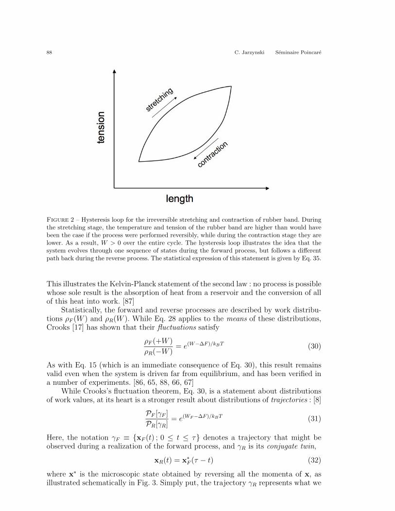
The second law of thermodynamics is manifested not only by inequalities suchas W ≥ ∆F , but also by the time-asymmetry inherent to irreversible processes.Hysteresis loops neatly depict this asymmetry. As an example, imagine that we ra-pidly stretch an ordinary rubber band, then after a sufficient pause we contract it,returning to the initial state. For this process we get a classic hysteresis loop byplotting the tension T versus the length L of the rubber band (Fig. 2). Hysteresisconveys the idea that the state of the rubber band follows one path during the stret-ching stage, but returns along a different path during contraction. Quantitatively,the second law implies that the enclosed area is non-negative,

∮T dL ≥ 0.

Similar considerations apply to the analogous stretching and contraction ofsingle molecules [86], only now statistical fluctuations become important : the ran-dom jigglings of the molecule differ from one repetition of the process to the next. Inthe previous section we saw that when fluctuations are taken into account, the rela-tionship between work and free energy can be expressed as an equality rather thanthe usual inequality. The central message of the present section has a similar ring :with an appropriate accounting of fluctuations, the two branches of an irreversiblethermodynamic cycle (e.g. the stretching and contraction of the single molecule) aredescribed by unexpected symmetry relations (Eqs. 30, 31) rather than exclusivelyby inherent asymmetry (Eqs. 28, 35).

To develop these results, it is useful to imagine two distinct processes, designatedthe forward and the reverse process. [8] The forward process is the one defined inSec. 2, in which the work parameter is varied from A to B using a protocol λF (t)(the subscript F has been attached as a label). During the reverse process, λ isvaried from B to A using the time-reversed protocol,

λR(t) = λF (τ − t). (27)

At the start of each process, the system is prepared in the appropriate equilibriumstate, corresponding to λ = A or B, at temperature T . If we perform the twoprocesses in sequence, the forward followed by the reverse, allowing the system toequilibrate with the reservoir at the end of each process, then we have a thermody-namic cycle that exhibits hysteresis. The Clausius inequality applies separately toeach stage :

−〈W 〉R ≤ ∆F ≤ 〈W 〉F (28)

where ∆F is defined as before (Eq. 5) and the notation now specifies separateaverages over the two processes. Of course, Eq. 28 implies that the average workover the entire cycle is non-negative,

〈W 〉F + 〈W 〉R ≥ 0. (29)


Figure 2 – Hysteresis loop for the irreversible stretching and contraction of rubber band. Duringthe stretching stage, the temperature and tension of the rubber band are higher than would havebeen the case if the process were performed reversibly, while during the contraction stage they arelower. As a result, W > 0 over the entire cycle. The hysteresis loop illustrates the idea that thesystem evolves through one sequence of states during the forward process, but follows a differentpath back during the reverse process. The statistical expression of this statement is given by Eq. 35.

This illustrates the Kelvin-Planck statement of the second law : no process is possiblewhose sole result is the absorption of heat from a reservoir and the conversion of allof this heat into work. [87]

Statistically, the forward and reverse processes are described by work distribu-tions ρF (W ) and ρR(W ). While Eq. 28 applies to the means of these distributions,Crooks [17] has shown that their fluctuations satisfy

ρF (+W )

ρR(−W )= e(W−∆F )/kBT (30)

As with Eq. 15 (which is an immediate consequence of Eq. 30), this result remainsvalid even when the system is driven far from equilibrium, and has been verified ina number of experiments. [86, 65, 88, 66, 67]

While Crooks’s fluctuation theorem, Eq. 30, is a statement about distributionsof work values, at its heart is a stronger result about distributions of trajectories : [8]

PF [γF ]

PR[γR]= e(WF−∆F )/kBT (31)

Here, the notation γF ≡ xF (t) ; 0 ≤ t ≤ τ denotes a trajectory that might beobserved during a realization of the forward process, and γR is its conjugate twin,

xR(t) = x∗F (τ − t) (32)

where x∗ is the microscopic state obtained by reversing all the momenta of x, asillustrated schematically in Fig. 3. Simply put, the trajectory γR represents what we


p

q

x (0)F

γF

γR

x ( )τF

x (0)R*x ( )τ

R*

Figure 3 – A conjugate pair of trajectories, γF and γR.

would see if we were to film the trajectory γF , and then run the movie backward.Eq. 31 then states that the probability of observing a particular trajectory whenperforming the forward process, PF [γF ], relative to that of observing its conjugatetwin during the reverse process, PR[γR], is given by the expression on the right sideof the equation, where WF ≡ W [γF ] is the work performed in the forward case.

To derive Eq. 31 for our toy model, assuming as before that the reservoir isremoved for 0 < t < τ , note that the ratio of probabilities to observe the Hamiltoniantrajectories γF and γR is simply the ratio of probabilities to sample their respectiveinitial conditions from equilibrium. [79] Thus

PF [γF ]

PR[γR]=ZB,TZA,T

e[H(xR(0);B)−H(xF (0);A)]/kBT

=ZB,TZA,T

e[H(xF (τ);B)−H(xF (0);A)]/kBT = e(WF−∆F )/kBT , (33)

using Eqs. 32 and 7 to replace H(xR(0);B) by H(xF (τ);B). We get to the finalresult by observing that the quantity inside square brackets on the second line is thenet change in H during the forward process, which (for a thermally isolated system,see Section 3) is the work performed on the system. As with the results of Section 3,numerous derivations of Eqs. 30 and 31 exist in the literature, corresponding tovarious models of the system and reservoir. [8, 17, 18, 52, 54, 89, 58, 59, 61, 62, 63, 32].

To gain some appreciation for this result, recall that a system in equilibriumsatisfies microscopic reversibility [90] (closely related to detailed balance [17]) : anysequence of events is as likely to occur as the time-reversed sequence. Using notationsimilar to Eq. 31 this condition can be written,

Peq[γ] = Peq[γ∗], (34)


where γ and γ∗ are a conjugate pair of trajectories (of some finite duration) for asystem in equilibrium. By contrast, as depicted by the two branches of a hysteresisloop, an essential feature of thermodynamic irreversibility is that the system doesnot simply retrace its steps when forced to return to its initial state. This idea isexpressed statistically by the inequality

PF [γF ] 6= PR[γR], (35)

that is the trajectories we are likely to observe during one process are not theconjugate twins of those we are likely to observe during the other process. Eq. 31,which replaces this inequality with a stronger equality, can be viewed as an extensionof the principle of microscopic reversibility, to systems that are driven away fromequilibrium by the variation of external parameters.

5 Relative entropy and dissipated work

Information theory and thermodynamics enjoy a special relationship, evidencedmost conspicuously by the formula,

I[peq] = S/kB, (36)

where I[p] ≡ −∫p ln p is the information entropy associated with a statistical dis-

tribution p. When p describes thermal equilibrium (Eq. 10), its information entropyI coincides with the thermodynamic entropy, S/kB (Eq. 36). This familiar but re-markable result relates a measure of our ignorance about a system’s microstate (I),to a physical quantity defined via calorimetry (S).

In recent years, another set of results have emerged that, similarly, draw aconnection between information theory and thermodynamics, but these results applyto irreversible processes rather than equilibrium states. Here the relevantinformation-theoretic measure is the relative entropy [91, 92] between two distribu-tions (Eq. 37), and the physical quantity is dissipated work, W −∆F . This sectiondescribes these results in some detail, but the central idea can be stated succinctlyas follows. The irreversibility of a process can be expressed as an inequality bet-ween a pair of probability distributions, either in trajectory space or in phase space(Eqs. 35, 40, 24). Using the relative entropy to quantify the difference between thetwo distributions, we find in each case that this measure relates directly to dissipatedwork (Eqs. 38, 41, 43).

For two normalized probability distributions p and q on the same space ofvariables, the relative entropy, or Kullback-Leibler divergence, [91]

D[p|q] ≡∫p ln

(p

q

)≥ 0 (37)

quantifies the extent to which one distribution differs from the other. D = 0 if andonly if the distributions are identical, and D 1 if there is little overlap betweenthe two distributions. Note that in general D[p|q] 6= D[q|p].

Because relative entropy provides a measure of distinguishability, it is a handytool for quantifying irreversibility. Recall that hysteresis can be expressed statisti-cally by the inequality PF [γF ] 6= PR[γR] (Eq. 35), where the trajectory-space distri-butions PF and PR represent the system’s response during the forward and reverse


processes. We can then use the relative entropy D[PF |PR] to assign a value to theextent to which the system’s evolution during one process differs from that duringthe other. From Eq. 31 it follows that [79]

D[PF |PR] =W dissF

kBT(38)

whereW dissF ≡ 〈W 〉F −∆F (39)

is the average amount of work that is dissipated during the forward process. (Simi-larly, D[PR|PF ] = W diss

R /kBT .)While distributions in trajectory space are abstract and difficult to visualize, a

result similar to Eq. 38 can be placed within the more familiar setting of phase space.Let fF (x, t) denote the time-dependent phase space density describing the evolutionof the system during the forward process (Eq. 22), and define fR(x, t) analogouslyfor the reverse process. Then the densities fF (x, t1) and fR(x, τ − t1) are snapshotsof the statistical state of the system during the two processes, both taken at themoment the work parameter achieves the value λ1 ≡ λF (t1) = λR(τ − t1). Theinequality

fF (x, t1) 6= fR(x∗, τ − t1) (40)

then expresses the idea that the statistical state of the system is different whenthe work parameter passes through the value λ1 during the forward process, thanwhen it returns through the same value during the reverse process. (The reversal ofmomenta in x∗ is related to the conjugate pairing of trajectories, Eq. 32.) Evaluatingthe relative entropy between these distributions, Kawai, Parrondo and Van denBroeck [93] found that

D[fF |f ∗R] ≤ W dissF

kBT, (41)

where the arguments of D are the distributions appearing in Eq. 40, for any choice ofλ1. This becomes an equality if the system is isolated from the thermal environmentas the work parameter is varied during each process. As with Eq. 38, we see that aninformation-theoretic measure of the difference between two distributions, fF andf ∗R, is related to a physical measure of dissipation, W diss

F /kBT .Eqs. 38 and 41 are closely related. The phase-space distribution fF = fF (x, t1) is

the projection of the trajectory-space distribution PF [γF ] onto a single “time slice”,t = t1, and similarly for f ∗R. Since the relative entropy between two distributionsdecreases when they are projected onto a smaller set of variables [91, 93] – in thiscase, from trajectory space to phase space – we have

D[fF |f ∗R] ≤ D[PF |PR] =W dissF

kBT. (42)

In the above discussion, relative entropy has been used to quantify the differencebetween the forward and reverse processes (hysteresis). It can equally well be usedto measure how far a system is removed from equilibrium at a given instant in time,leading again to a link between relative entropy and dissipated work (Eq. 43 below).

For the process introduced in Sec. 2, let ft ≡ f(x, t) denote the statistical state ofthe system at time t, and let peq

t ≡ peqλ(t),T (x) be the equilibrium state corresponding


to the current value of the work parameter. It is useful to imagine that ft continually“chases” peq

t : as the work parameter is varied with time, the state of the system (ft)tries to keep pace with the changing equilibrium distribution (peq

t ), but is unable todo so (except in the reversible, isothermal limit). Vaikuntanathan and Jarzynski [94]have shown that

D[ft|peqt ] ≤ 〈w(t)〉 −∆F (t)

kBT(43)

where ∆F (t) ≡ Fλ(t),T − FA,T . In other words, the average work dissipated up totime t, in units of kBT , provides an upper bound on the degree to which the systemlags behind equilibrium at that instant. This result can be obtained from eitherEq. 25 or Eq. 41. [94] If we take t = τ ∗, allowing the system to relax to a final stateof equilibrium (see Sec. 2.1), then the left side of Eq. 43 vanishes and once again werecover the Clausius inequality.

As mentioned, relative entropy is an asymmetric measure : in general D[p|q] 6=D[q|p]. Feng and Crooks [95] have discussed the use of two symmetric measures ofdistinguishability to quantify thermodynamic irreversibility. The first is the Jeffreysdivergence, D[p|q] + D[q|p]. When applied to forward and reverse distributions intrajectory space, this gives the average work over the entire cycle (see Eq. 38) :

Jeffreys(PF ;PR) =W dissF +W diss

R

kBT=〈W 〉F + 〈W 〉R

kBT. (44)

The second measure is the Jensen-Shannon divergence,

JS(p; q) =1

2(D[p|m] +D[q|m]) , (45)

where m = (p + q)/2 is the mean of the two distributions. When evaluated withp = PF and q = PR, this leads to a more complicated, nonlinear average of W diss

F

and W dissR (see Eq. 7 of Ref. [95]). Feng and Crooks nevertheless argue that the

Jensen-Shannon divergence is the preferred measure of time-asymmetry, as it has aparticularly nice information-theoretic interpretation. I will return to this point atthe end of the following section.

6 Guessing the direction of time’s arrow

Sir Arthur Eddington introduced the term “arrow of time” to describe theevident directionality associated with the flow of events. [96] While time’s arrowis familiar from daily experience – everyone recognizes that a movie run backwardlooks peculiar ! – Eddington (among others) argued that it is rooted in the secondlaw of thermodynamics. For a macroscopic system undergoing an irreversible processof the sort described in Sec. 2.1, the relationship between the second law and thearrow of time is almost tautological : W > ∆F when events proceed in the correctorder, and W < ∆F when the movie is run backward, so to speak. For a microscopicsystem, fluctuations blur this picture, since we can occasionally observe violationsof the Clausius inequality (Eq. 5). Thus the sign of W −∆F , while correlated withthe direction of time’s arrow, does not fully determine it. These general observationscan be made precise, that is the ability to determine the direction of time’s arrowcan be quantified.


To discuss this point, it is convenient to consider a hypothetical guessing game[79]. Imagine that I show you a movie in which you observe a system undergoinga thermodynamic process as λ is varied from A to B. Your task is to guess whe-ther this movie depicts the events in the order in which they actually occurred, orwhether I have filmed the reverse process (varying λ from B to A) and am now(deviously) showing you the movie of that process, run backward. In the spirit of aGedankenexperiment, assume that the movie gives you full microscopic informationabout the system – you can track the motion of every atom – and that you know theHamiltonian function H(x;λ) and the value ∆F = FB,T − FA,T . Assume moreoverthat in choosing which process to perform, I flipped a fair coin : heads = F , tails= R.

We can formalize this task as an exercise in statistical inference. [95] Let L(F |γ)denote the likelihood that the movie is being shown in the correct direction (i.e. thecoin landed on heads and the forward process was performed), given the microscopictrajectory γ that you observe in the movie. Similarly, let L(R|γ) denote the likelihoodthat the reverse process was in fact performed and the movie is now being runbackward. Since these are the only possibilities, the likelihoods associated with thetwo hypotheses (F , R) sum to unity :

L(F |γ) + L(R|γ) = 1 (46)

Now let W denote the work performed on the system, for the trajectory depictedin the movie. If W > ∆F , then the first hypothesis (F ) is in agreement with theClausius inequality, while the second hypothesis (R) is not ; if W < ∆F , it is theother way around. Therefore for a macroscopic system the task is easy, as the signof W −∆F determines the direction of time’s arrow. Formally,

L(F |γ) = θ(W −∆F ) (47)

where θ(·) is the unit step function.For a microscopic system we must allow for the possibility that Eq. 5 might be

violated now and again. Bayes’ Theorem then provides the right tool for analyzingthe likelihood :

L(F |γ) =P (γ|F )P (F )

P (γ). (48)

Here P (F ) is the prior probability that I carried out the forward process, whichis simply 1/2 since I flipped a fair coin to make my choice, and P (γ|F ) is theprobability to generate the trajectory γ when performing the forward process ; inthe notation of Sec. 4, this is PF [γ]. Finally, P (γ) is (effectively) a normalizationconstant. Writing the analogous formula for L(R|γ), then combining these with thenormalization condition Eq. 46 and invoking Eq. 31, we get [97, 98, 31]

L(F |γ) =1

1 + e−(W−∆F )/kBT. (49)

This result quantifies your ability to determine the arrow of time from the trajectorydepicted in the movie. The expression on the right is a smoothed step function. Ifthe W surpasses ∆F by many units of kBT , then L(F |γ) ≈ 1 and you can say withhigh confidence that the movie is being shown in the correct direction, while in theopposite case you can be equally confident that the movie is being run backward.


The transition from one regime to the other – where time’s arrow gets blurred, inessence – occurs over an interval of work values whose width is a few kBT . (Indeed,when viewed from a distance – that is, when plotted as a function of W on an axiswith macroscopic units of energy – Eq. 49 is indistinguishable from Eq. 47.) What isremarkable is that this transition does not depend on the details of either the systemor the protocol λ(t). Eq. 49 was derived by Shirts et al [97] and later by Maragakis etal [98] in the context of free energy estimation, where the interpretation is somewhatdifferent from the one I have discussed here.

Finally, returning to the point mentioned at the end of the previous section,the Jensen-Shannon divergence has the following interpretation in the context ofour hypothetical guessing game : JS(PF ;PR) is the average gain in information(regarding which process was performed) obtained from observing the movie [95].When the processes are highly irreversible, this approaches its maximum value,JS ≈ ln 2, corresponding to one bit of information. This makes sense : by watchingthe movie you are able to infer with confidence whether the coin I flipped turned upheads (F ) or tails (R). Feng and Crooks [95] have argued that this interpretation hassurprisingly universal implications for biomolecular and other nanoscale machines.Namely, about 4 − 8 kBT of free energy must be dissipated per operating cycle toguarantee that the machine runs reliably in a designated direction (as opposed totaking backward and forward steps with equal probability, as would necessarily occurunder equilibrium conditions).

Finally, time’s arrow has unexpected relevance for the convergence of the expo-nential average in Eq. 15. Namely, the realizations that dominate that average areprecisely those “during which the system appears as though it is evolving backwardin time”. [79] A detailed analysis of this assertion involves both hysteresis and re-lative entropy, thus nicely tying together the four strands of discussion representedby Sections 3 – 6. [79]

7 Entropy production and related quantities

This review has focused on far-from-equilibrium predictions for work and freeenergy (Eqs. 15, 25, 30, 31) and how these inform our understanding of irreversibi-lity and the second law of thermodynamics. Because the second law is often takento be synonymous with the increase of entropy, we might well wonder how thesepredictions relate to statements about entropy.

As a point of departure, for macroscopic systems we can use the first law (∆U =W +Q) and the definition of free energy (F = U − ST ) to write,

W −∆F

T= ∆S − Q

T= ∆Stot, (50)

where ∆Stot is the combined entropy change of the system and reservoir. If we extendthis to microscopic systems, accepting it as the definition of ∆Stot for a single reali-zation of a thermodynamic process, then the results discussed in Sections 3 - 6 canformally be rewritten as statements about the fluctuations of entropy production.

When multiple thermal reservoirs are involved, one can generalize Eq. 6 in anobvious way by including terms for all the reservoirs, e.g. H = H+

∑k(H

kenv +Hk

int).Working entirely within a Hamiltonian framework, the results of Sec. 3, notablyEqs. 15, 19 and 20, can then be written in terms of entropy production, and ge-neralized further by dropping the assumption that the system of interest begins in


equilibrium. [99] Esposito, Lindenberg and Van den Broeck have recently shownthat in this situation the value of ∆Stot is equal to the statistical correlation thatdevelops between the system and the reservoirs, as measured in terms of relativeentropy. [100]

The Hamiltonian framework is often inconvenient for studying nonequilibriumsteady states. Among the many tools that have been introduced for the theoreticalanalysis and numerical simulation of such states, Gaussian thermostats – the termrefers to a method of modeling nonequilibrium systems based on Gauss’s principleof least constraint [101] – have played a prominent role in recent developmentsin nonequilibrium thermodynamics. The term fluctuation theorem was originallyapplied to a property of entropy production, observed in numerical investigationsof a sheared fluid simulated using a Gaussian thermostat [10, 11, 12, 13]. Sincefluctuation theorems for entropy production have been reviewed elsewhere [21, 22,24, 29, 30, 32, 33, 35, 36], I will limit myself to a brief summary of how these resultsconnect to those of Sections 3 - 6.

The transient fluctuation theorem of Evans and Searles [11] applies to a systemthat evolves from an initial state of equilibrium to a nonequilibrium steady state.Letting pτ (∆s) denote the probability distribution of the entropy produced up to atime τ > 0, it states that

pτ (+∆s)

pτ (−∆s)= e∆s/kB . (51)

This is clearly similar to Eq. 30, except that it pertains to a single thermodynamicprocess, rather than a pair of processes (F and R). Eq. 51 implies an integratedfluctuation theorem,

〈e−∆s/kB〉 = 1, (52)

that is entirely analogous to Eq. 15, and from this we in turn get analogues of Eqs. 19and 20 :

〈∆s〉 ≥ 0 , P [∆s < −ξ] ≤ e−ξ/kB (53)

Now consider a system that is in a nonequilibrium steady state from the distantpast to the distant future, such as a fluid under constant shear [10], and let σ ≡∆s/τ denote the entropy production rate, time-averaged over a single, randomlysampled interval of duration τ . The steady-state fluctuation theorem of Gallavottiand Cohen [12, 13] asserts that the probability distribution pτ (σ) satisfies

limτ→∞

1

τlnpτ (+σ)

pτ (−σ)=

σ

kB. (54)

The integrated form of this result is [21]

limτ→∞

1

τln⟨e−τσ/kB

⟩τ

= 0, (55)

where the brackets denote an average over intervals of duration τ , in the steadystate. Formal manipulations then give us

〈σ〉τ ≥ 0 , limτ→∞

1

τlnPτ [σ < −ε] ≤ −ε, (56)

where Pτ [σ < −ε] is the probability to observe a time-averaged entropy productionrate less than −ε, during an interval of duration τ . The resemblance between Eqs. 54


- 56, and Eqs. 30, 15, 19, 20, respectively, should be obvious, although viewed asmathematical statements they are different.

The microscopic definition of entropy production in Eqs. 51 - 56 depends on theequations of motion used to model the evolution of the system. In the early papers onfluctuation theorems, entropy production was identified with phase space contractionalong a deterministic but non-Hamiltonian trajectory [10, 11, 12, 13]. These resultswere then extended to encompass stochastic dynamics, first by Kurchan [14] fordiffusion, and then by Lebowitz and Spohn [15] for Markov processes in general.Maes subsequently developed a unified framework based on probability distributionsof “space-time histories” [16], that is trajectories. In all these cases, the validity ofthe fluctuation theorem ultimately traces back to the idea that trajectories comein pairs related by time-reversal, and that the production of entropy is intimatelylinked with the probability of observing one trajectory relative to the other, in amanner analogous with Eq. 31.

As an aside, it is intriguing to note that multiple fluctuation theorems can bevalid simultaneously, in a given physical context. This idea was mentioned in passingby Hatano and Sasa [19] in the context of transitions between nonequilibrium states,and has been explored in greater detail by a number of authors since then [54, 103,32, 104].

Finally, for nonequilibrium steady states there exist connections between rela-tive entropy and entropy production, analogous to those discussed in Sec. 5. If rela-tive entropy is used to quantify the difference between distributions of steady-statetrajectories and their time-reversed counterparts, then the value of this differencecan be equated with the thermodynamic production of entropy. This issue has beenexplored by Maes [16], Maes and Netocny [105], and Gaspard [106].

8 Conclusions and Outlook

The central message of this review is that far-from-equilibrium fluctuations aremore interesting than one might have guessed : they tell us something new abouthow the second law of thermodynamics operates at the nanoscale. In particular,they allow us to rewrite thermodynamic inequalities as equalities, and they revealthat nonequilibrium fluctuations encode equilibrium information.

The last observation has led to practical applications in two broad settings.The first is the development of numerical methods for estimating free energy dif-ferences, an active enterprise in computational chemistry and physics. [23] Whiletraditional strategies involve equilibrium sampling, Eqs. 15, 25 and 30 suggest theuse of nonequilibrium simulations to construct estimates of ∆F . This is an ongoingarea of research [107, 108], but nonequilibrium methods have gradually gained ac-ceptance into the free energy estimation toolkit, and are being applied to a varietyof molecular systems ; see Ref. [109] for a recent example.

Nonequilibrium work relations have also been applied to the analysis of single-molecule experiments, as originally proposed by Hummer and Szabo [9] and pionee-red in the laboratory by Liphardt et al. [64] Individual molecules are driven awayfrom equilibrium using (for instance) optical tweezers or atomic-force microscopy,and from measurements of the work performed on these molecules, one can recons-truct equilibrium free energies of interest. [27, 110] For recent applications of thisapproach, see Refs. [111, 112, 113, 114].


It remains to be seen whether the understanding of far-from-equilibrium fluc-tuations that has been gained in recent years will lead to the formulation of a unified“thermodynamics of small systems”, that is, a theoretical framework based on a fewpropositions, comparable to classical thermodynamics. Some progress, however, hasbeen made in this direction.

For stochastic dynamics, Seifert and colleagues [54, 115, 116, 117, 32] – buildingon earlier work by Sekimoto [118, 37] – have developed a formalism in which micro-scopic analogues of all relevant macroscopic quantities are precisely defined. Many ofthe results discussed in this review follow naturally within this framework, and thishas helped to clarify the relations among these results. [32] Evans and Searles [22]have championed the view that fluctuation theorems are most naturally understoodin terms of a dissipation function, Ω, whose properties are (by construction) inde-pendent of the dynamics used to model the system of interest. More recently, Ge andQian [119] have proposed a unifying framework for stochastic processes, in whichboth the information entropy −

∫p ln p and the relative entropy

∫p ln(p/q) play key

roles.References [32] and [119] make a connection to earlier efforts by Oono and

Paniconi [120] to develop a “steady-state thermodynamics” organized around none-quilibrium steady states. While the original goal was a phenomenological theory, thederivation by Hatano and Sasa of fluctuation theorems for transitions between steadystates [19, 121] has encouraged a microscopic approach to this problem. [122, 123]In the absence of a universal statistical description of steady states analogous to theBoltzmann-Gibbs formula (Eq. 10) this has proven to be highly challenging.

This review has focused exclusively on classical fluctuation theorems and workrelations, but the quantum case is also of considerable interest. While quantumversions of these results have been studied for some time [124, 125, 126, 127], thepast two to three years have seen a surge of interest in this topic [128, 129, 130,131, 132, 133, 134, 135, 136, 137, 138, 139, 140, 141, 142]. Quantum mechanicsof course involves profound issues of interpretation. It can be hoped that in theprocess of trying to specify the quantum-mechanical definition of work [132], ordealing with open quantum systems [131, 137, 138, 139, 140, 141, 142], or analyzingexactly solvable models [130, 133, 135, 136], or proposing and ultimately performingexperiments to test far-from-equilibrium predictions [134], important insights will begained. Applications of nonequilibrium work relations to the detection of quantumentanglement [143] and to combinatorial optimization using quantum annealing [144]have very recently been proposed.

Finally, there has been a rekindled interest in recent years in the thermodyna-mics of information-processing systems and closely related topics such as the appa-rent paradox of Maxwell’s demon [145]. Making use of the relations described in thisreview, a number of authors have investigated how nonequilibrium fluctuations andthe second law are affected in situations involving information processing, such asoccur in the context of memory erasure and feedback control. [146, 147, 148, 149, 150]

Acknowledgments

I gratefully acknowledge financial support from the National Science Foundation(USA), under DMR-0906601. This article will appear in Annu. Rev. Cond. Mat.Phys.


References

[1] Kolomeisky AB., Fisher ME.: Annu. Rev. Phys. Chem. 58, 675–95 (2006).

[2] Smith DE., Tans SJ., Smith SB., Grimes S., Anderson DL., Bustamante C.:Nature 413, 748–52 (2001).

[3] Bustamante C., Liphardt J., Ritort F.: Phys. Today 58 (July), 43–48 (2005).

[4] Bochkov GN., Kuzovlev YuE.: Zh. Eksp. Teor. Fiz. 72, 238–47 (1977).

[5] Bochkov GN., Kuzovlev YuE.: Zh. Eksp. Teor. Fiz. 76, 1071 (1979).

[6] Jarzynski C.: Phys. Rev. Lett. 78, 2690–2693 (1997).

[7] Jarzynski C.: Phys. Rev. E 56, 5018–5035 (1997).

[8] Crooks GE.: J. Stat. Phys. 90, 1481–87 (1998).

[9] Hummer G., Szabo A.: 2001. Proc. Natl. Acad. Sci. (USA) 98, 3658–61 (2001).

[10] Evans DJ., Cohen EGD., Morriss GP.: Phys. Rev. Lett. 71, 2401–04 (1993).

[11] Evans DJ., Searles DJ.: Phys. Rev. E 50, 1645–48 (1994).

[12] Gallavotti G., Cohen EGD.: Phys. Rev. Lett. 74, 2694–97 (1995).

[13] Gallavotti G., Cohen EGD.: J. Stat. Phys. 80, 931–970 (1995).

[14] Kurchan J.: J. Phys. A: Math. Gen. 31, 3719–29 (1998).

[15] Lebowitz JL., Spohn H.: J. Stat. Phys. 95, 333–65 (1999).

[16] Maes C.: J. Stat. Phys. 95, 367–92 (1999).

[17] Crooks GE.: Phys. Rev. E 60, 2721–26 (1999).

[18] Crooks GE.: Phys. Rev. E 61, 2361–66 (2000).

[19] Hatano T., Sasa S-I.: Phys. Rev. Lett. 86, 3463–66 (2001).

[20] Adib AB.: Phys. Rev. E 71, 056128/1–5 (2005).

[21] Gallavotti G.: Statistical Mechanics: A Short Treatise. Springer-Verlag, Berlin(1999).

[22] Evans DJ., Searles DJ.: Adv. Phys. 51, 1529–85 (2002).

[23] Frenkel D., Smit B.: Understanding Molecular Simulation: From Algorithmsto Applications. Academic Press, San Diego (2002).

[24] Maes C.: Seminaire Poincare 2, 29–62 (2003).

[25] Ritort F.: Seminaire Poincare 2, 193–226 (2003).

[26] Hummer G., Szabo A.: Acc. Chem. Res. 38, 504–13 (2005).

[27] Ritort F.: J. Phys.: Condens. Matter 18, R531–83 (2006).

[28] Kurchan J.: J. Stat. Mech.: Theory and Experiment P07005/1–14 (2007).

[29] Harris RJ., Schutz G. M.: J. Stat. Mech.: Theory and Experiment P07020/1–45(2007).

[30] Gallavotti G.: Eur. Phys. J. B 64, 315–20 (2008).

[31] Jarzynski C.: Eur. Phys. J. B 64, 331–40 (2008).

[32] Seifert U.: 2008. Eur. Phys. J. B 64, 423–431 (2008).

[33] Sevick EM., Prabhakar R., Williams SR., Searles DJ.: Annu. Rev. Phys. Chem.59, 603–33 (2008).


[34] Evans DJ., Morriss G.: Statistical Mechanics of Nonequilibrium Liquids. 2nded. Cambridge University Press, Cambridge (2008).

[35] Esposito M., Harbola U., Mukamel S.: 2009. Rev. Mod. Phys. 81, 1665–1702(2009).

[36] Kurchan J.: Lecture Notes of the Les Houches Summer School: Volume 90,August 2008 (arXiv:0901.1271v2) (2010).

[37] Sekimoto K.: Stochastic Energetics. Lecture Notes in Physics 799. Springer,Berlin (2010).

[38] Boksenbojm E., Wynants B., Jarzynski C.: Physica A (2010), (in press)

[39] Finn CBP.: Thermal Physics. 2nd ed. Chapman and Hall, London (1993).

[40] Uhlenbeck GE., Ford GW.: Lectures in Statistical Mechanics. American Math-ematical Society, Providence (1963). Chapter 1, Section 7.

[41] Jarzynski C.: Acta Phys. Pol. B 29, 1609–22 (1998).

[42] Jarzynski C.: C. R. Physique 8, 495–506 (2007).

[43] Vilar JMG., Rubi JM.: Phys. Rev. Lett. 100, 020601/1–4 (2008).

[44] Peliti L.: J. Stat. Mech.: Theory and Experiment P05002/1–9 (2008).

[45] Peliti L.: Phys. Rev. Lett. 101, 098901 (2008).

[46] Vilar JMG., Rubi JM.: Phys. Rev. Lett. 101, 098902 (2008).

[47] Horowitz J., Jarzynski C.: Phys. Rev. Lett. 101, 098903 (2008).

[48] Vilar JMG., Rubi JM.: Phys. Rev. Lett. 101, 098904 (2008).

[49] Zimanyi EN., Silbey RJ.: J. Chem. Phys. 130, 171102/1–3 (2009).

[50] Jarzynski C.: J. Stat. Mech.: Theory and Experiment P09005/1–13 (2004).

[51] Sun SX.: J. Chem. Phys. 118, 5769–75 (2003).

[52] Evans DJ.: Mol. Phys. 101, 1551–45 (2003).

[53] Imparato A., Peliti L.: Europhys. Lett. 70, 740–46 (2005).

[54] Seifert U.: Phys. Rev. Lett. 95, 040602/1–4 (2005).

[55] Oberhofer H., Dellago C., Geissler PL.: J. Chem. Phys. 109, 6902–15 (2005).

[56] Cuendet MA.: Phys. Rev. Lett. 96, 120602/1–4 (2006).

[57] Cuendet MA.: J. Chem. Phys. 125, 144109/1–12 (2006).

[58] Scholl-Paschinger E., Dellago C.: J. Chem. Phys. 125, 054105/1–5 (2006).

[59] Chelli R., Marsili S., Barducci A., Procacci P.: 2007. Phys. Rev. E 75,050101(R)/1–4 (2007).

[60] Ge H., Qian M.: J. Math. Phys. 48, 053302/1–11 (2007).

[61] Ge H., Jiang D-Q.: J. Stat. Phys. 131, 675–89 (2008).

[62] Williams SR., Searles DJ., Evans DJ.: Phys. Rev. Lett. 100, 250601/1–4 (2008).

[63] Chetrite R., Gawedzki K.: Commun. Math. Phys. 282, 469–518 (2008).

[64] Liphardt J., Dumont S., Smith SB., Tinoco I Jr., Bustamante C.: Science 296,1832–35 (2002).

[65] Douarche F., Ciliberto S., Petrosyan A.: J. Stat. Mech.: Theory and Experi-ment P09011/1–18 (2005).


[66] Blickle V., Speck T., Helden L., Seifert U., Bechinger C.: Phys. Rev. Lett. 96,070603/1–4 (2006).

[67] Douarche F., Ciliberto S., Petrosyan A., Rabbiosi I.: Europhys. Lett. 70, 593–99 (2005).

[68] Goldstein H.: Classical Mechanics. 2nd ed. Addison-Wesley, Reading, Mas-sachusetts (1980).

[69] Bochkov GN., Kuzovlev YuE.: Physica A 106, 443–79 (1981).

[70] Bochkov GN., Kuzovlev YuE.: Physica A 106, 480–520 (1981).

[71] Horowitz J., Jarzynski C.: J. Stat. Mech.: Theory and Experiment P11002/1–14 (2007).

[72] Chandler D.: Introduction to Modern Statistical Mechanics. section 5.5. Ox-ford University Press, New York (1987).

[73] Hermans J.: J. Phys. Chem. 114, 9029–32 (1991).

[74] Wood RH., Muhlbauer CF., Thompson PT.: J. Phys. Chem. 95, 6670–75(1991).

[75] Hendrix DA., Jarzynski C.: J. Chem. Phys. 114, 5974–81 (2001).

[76] Speck T., Seifert U.: Phys. Rev. E 70, 066112/1–4 (2004).

[77] Cohen EGD., Berlin TH.: Physica 26, 717–29 (1960).

[78] Evans DJ., Searles DJ.: Phys Rev E 53, 5808–15 (1996).

[79] Jarzynski C.: Phys. Rev. E 73, 046105/1–10 (2006).

[80] Gibbs JW.: Elementary Principles in Statistical Mechanics. Scribner’s, NewYork (1902).

[81] Campisi M.: Studies in History and Philosophy of Modern Physics 39, 181–94(2008).

[82] Sato K.: J. Phys. Soc. Japan 71, 1065–66 (2002).

[83] Marathe R., Parrondo JMR.: arXiv:0909.0617v2, (2010).

[84] Jarzynski C.: Proc. Natl. Acad. Sci. (USA) 98, 3636–38 (2001).

[85] Berkovich R., Klafter J., Urbakh M.: J. Phys.: Condens. Matter 20, 345008/1–7(2008).

[86] Collin D., Ritort F., Jarzynski C., Smith SB., Tinoco I. Jr., Busamante C.:Nature 437, 231–34 (2005).

[87] Planck M.: 1927. Treatise on Thermodynamics, 3rd ed. (translated from 7thGerman edition). Longmans, Green and Co., Inc., London. Page 89, (1927),(Dover edition, 1945).

[88] Douarche F., Joubaud S., Garnier NB., Petrosyan A., Ciliberto S.: Phys. Rev.Lett. 97, 140603/1–4 (2006).

[89] Cleuren B., Van den Broeck C., Kawai R.: Phys. Rev. Lett. 96, 050601/1–4(2006).

[90] Tolman RC.: Proc. Natl. Acad. Sci. (USA) 11, 436-39 (1925).

[91] Cover TM., Thomas JA.: Elements of Information Theory. John Wiley andSons, Inc. New York (1991).


[92] Qian H.: Phys. Rev. E 63, 042103/1–4 (2001).

[93] Kawai R., Parrondo JMR., Van den Broeck C.: Phys. Rev. Lett. 98, 080602/1–4 (2007).

[94] Vaikuntanathan S., Jarzynski C.: EPL 87, 60005/1–6 (2009).

[95] Feng EH., Crooks, GE.: Phys. Rev. Lett. 101, 090602/1–4 (2008).

[96] Eddington AS.: The Nature of the Physical World. Macmillan (1928).

[97] Shirts ME., Bair E., Hooker G., Pande VS.: Phys. Rev. Lett. 91, 140601/1–4(2003).

[98] Maragakis P., Ritort F., Bustamante C., Karplus M., Crooks GE.: J. Chem.Phys. 129, 024102/1–8 (2008).

[99] Jarzynski C.: J. Stat. Phys. 96, 415–27 (1999).

[100] Esposito M., Lindenberg K., Van den Broeck C.: New J. Phys. 12, 013013/1–10(2010).

[101] Evans DJ., Hoover WG., Failor BH., Moran B., Ladd AJC.: Phys. Rev. A 28,1016–21 (1983).

[102] Touchette H.: Phys. Reports 478, 1–69 (2009).

[103] Chernyak VY., Chertkov M., Jarzynski C.: J. Stat. Mech.: Theory and Exper-iment P08001/1–19 (2006).

[104] Esposito M., Van den Broeck C.: Phys. Rev. Lett. 104, 090601/1–4 (2010).

[105] Maes C., Netocny K.: J. Stat. Phys. 110, 269–310 (2003).

[106] Gaspard P.: J. Stat. Phys. 117, 599–615 (2004).

[107] Park S., Schulten K.: J. Chem. Phys. 120, 5946–61 (2004).

[108] Chipot C., Pohorille A.: Free Energy Calculations. Springer, Berlin (2007).

[109] Chami F., Wilson MR.: J. Am. Chem. Soc. 132, 7794–7802 (2010).

[110] Bustamante C.: Quar. Rev. Biophys. 38, 291–301 (2005).

[111] Harris NC., Song Y., Kiang C-H.: Phys. Rev. Lett. 99, 068101/1–4 (2007).

[112] Greenleaf WJ., Frieda KL., Foster DAN., Woodside MT., Block SM.: Science319, 630–33 (2008).

[113] Junier I., Mossa A., Manosas M., Ritort F.: Phys. Rev. Lett. 102, 070602/1–4(2009).

[114] Shank EA., Cecconi C., Dill JW., Marqusee S., Bustamante C.: Nature 465,637–41 (2010).

[115] Speck T., Seifert U.: J. Phys. A: Math. Gen. 38, L581–88 (2005).

[116] Schmiedl T., Seifert U.: J. Chem. Phys. 126, 044101/1–12 (2007).

[117] Schmiedl T., Speck T., Seifert U.: J. Stat. Phys. 128, 77–93 (2007).

[118] Sekimoto K.: Prog. Theor. Phys. Suppl 130, 17–27 (1998).

[119] Ge H., Qian H.: Phys. Rev. E 81, 051133/1–5 (2010).

[120] Oono Y., Paniconi M.: Prog. Theor. Phys. Suppl 130, 29–44 (1998).

[121] Trepagnier EH., Jarzynski C., Ritort F., Crooks GE., Bustamante CJ.,Liphardt J.: Proc. Natl. Acad. Sci. (USA) 101, 15038–41 (2004).


[122] Komatsu TS., Nakagawa N., Sasa S-I., Tasaki H.: Phys. Rev. Lett. 100,230602/1–4 (2008).

[123] Komatsu TS., Nakagawa N., Sasa S-I., Tasaki H.: J. Stat. Phys. 134, 401–23(2009).

[124] Yukawa S.: J. Phys. Soc. Japan 69, 2367–70 (2000).

[125] Kurchan J.: arXiv:cond-mat/0007360v2, (2000).

[126] Tasaki H.: arXiv:cond-mat/0009244v2, (2000).

[127] Mukamel S.: Phys. Rev. Lett. 90, 170604/1–4 (2003).

[128] Talkner P., Lutz E., Hanggi P.: Phys. Rev. E 75, 050102(R)/1–2 (2007).

[129] Talkner P., Hanggi P.: J. Phys. A: Math. Theor. 40, F569–71 (2007).

[130] Teifel J., Mahler G.: Phys. Rev. E 76, 051126/1–6 (2007).

[131] Quan HT., Yang S., Sun CP.: arXiv:0804.1312v1, (2008).

[132] Talkner P., Hanggi P., Morillo M.: Phys. Rev. E 77, 051131/1–6 (2008).

[133] Talkner P., Burada PS., Hanggi P.: Phys. Rev. E 78, 011115/1–11 (2008).

[134] Huber G., Schmidt-Kaler S., Deffner S., Lutz E.: Phys. Rev. Lett. 101,070403/1–4 (2008).

[135] Van Zon R., Hernandez de la Pena L., Peslherbe GH., Schofield J.: Phys. Rev.E 78, 041103/1–11 (2008).

[136] Van Zon R., Hernandez de la Pena L., Peslherbe GH., Schofield J.: Phys. Rev.E 78, 041104/1–14 (2008).

[137] Crooks GE.: J. Stat. Mech.: Theor. Experiment P10023/1–9 (2008).

[138] Quan HT., Dong H.: arXiv:0812.4955v1, (2008).

[139] Talkner P., Campisi M., Hanggi P.: J. Stat. Mech.: Theor. ExperimentP02025/1–12 (2009).

[140] Deffner S., Lutz E.: arXiv:0902.1858v1, (2009).

[141] Andrieux D., Gaspard P., Monnai T., Tasaki S.: New J. Phys. 11, 043014/1–25(2009).

[142] Campisi M., Talkner P., Hanggi P.: Phys. Rev. Lett. 102, 210401/1–4 (2009).

[143] Hide J., Vedral V.: 2010. Phys. Rev. A 81, 062303/1–5 (2010).

[144] Ohzeki M.: Phys. Rev. Lett., in press (2010).

[145] Maruyama K., Nori F., Vedral V.: Rev. Mod. Phys. 81, 1–23 (2009).

[146] Piechocinska B.: Phys. Rev. A 61, 062314/1–9 (2000).

[147] Sagawa T., Ueda M.: Phys. Rev. Lett. 100, 080403/1–4 (2008).

[148] Dillenschneider R., Lutz E.: Phys. Rev. Lett. 102, 210601/1–4 (2009).



equalities and inequalities : irreversibility and the second law of

Documents