COVER SHEET

Akintoye, A.S. and Skitmore, Martin R. (1994) A comparative analysis of three macro price forecasting models. Construction Management and Economics 12(3):pp. 257-270. Copyright 1994 Taylor and Francis. Accessed from: http://eprints.qut.edu.au/archive/00004407/

A COMPARATIVE ANALYSIS OF THREE MACRO PRICE FORECASTING MODELS Paper prepared for Construction Management and Economics by Dr S A Akintoye Department of Building and Surveying Glasgow Caledonian University Glasgow, Scotland and Prof R M Skitmore Department of Surveying University of Salford Salford M5 4WT, England Telephone: 061 745 5225 REVISED PAPER: REF 511 October, 1993

A COMPARATIVE ANALYSIS OF THREE MACRO PRICE FORECASTING SYSTEMS

Akintola Akintoye and Martin Skitmore

ABSTRACT

This paper examines the relative performance of three different

systems of forecasting movements in macro building prices. The

three systems analysed are (1) the Building Cost Information

Service system, (2) the Davis, Langdon & Everest system, and (3)

Akintoye and Skitmore's reduced-form simultaneous equation. A

battery of accuracy measures are used to compare the forecasts

published by the Building Cost Information Service and Davis,

Langdon & Everest systems and simulated out-sample forecasts

made by the Akintoye and Skitmore system. The results indicate

that, during the three year period commencing with the first

quarter 1988, the Akintoye and Skitmore system gives the most

accurate forecasts for a zero to three quarters forecast horizon

and the Building Cost Information Service system gives the most

accurate forecasts for a four to eight quarters forecast

horizon.

Keywords: Tender Price Index, forecasting, econometrics,

accuracy.

2

INTRODUCTION

A major objective of construction management and economics

research is to improve the quality of decision making in the

industry. One way of achieving this is to find means of

improving the quality of information available to decision

makers concerning the likely outcomes of potential decisions.

For economic and investment decisions, forecasts are needed of

future price levels. Macro price forecasts are currently

available in the form of a tender price index (TPI) from several

systems. Little is known of the forecasting accuracy of these

systems or of the impact of economic circumstances on this

accuracy to enable decision makers to fully appreciate each

systems limitations or select one to use.

This paper describes an analysis of the reliability and

forecasting behaviour of three of these systems - (1) The Royal

Institution of Chartered Surveyors' Building Cost Information

Services's (BCIS) system, (2) the Davis, Langdon & Everest

(DL&E) system, and (3) Akintoye and Skitmore's (1993) reduced-

form simultaneous equation (A&S). The BCIS and DL&E systems

were chosen for comparison purposes because: apart from the

Property Services Agency Specialist Services (Directorate of

Building Surveying Services) these are the two most established

organisations in forecasting construction price movements, with

activities dating back to 1980 and 1976 respectively; and both

are private sector organisations and both forecast movements in

3

tender price relating to both public and private construction

work. The tender price forecasts of these two organisations

should therefore be a good reflection of the genuine competitive

situation in the construction industry.

The A&S equation is one of two recently developed econometric

models of macro building prices. In their paper, Akintoye and

Skitmore (1993) present a reduced form simultaneous equation

model to explain general movements and a single structural

equation model, based on economic theory, to explain structural

TPI movements. Both models were found to fit the BCIS TPI well.

Single structural models however are known to have an inferior

predictive power to reduced-form equations (Kane, 1968:21-2;

Neal and Shone 1976) and therefore the reduced-form equation has

been adopted in this analysis.

A battery of accuracy measures is described and these are

applied to the forecasts provided by the systems for comparative

purposes. For the period examined, the results indicate that

the Akintoye and Skitmore system gives the most accurate

forecasts for a zero to three quarters forecast horizon and the

Building Cost Information Service system gives the most accurate

forecasts for a four to eight quarters forecast horizon.

4

MODELS, FORECASTING AND ERRORS

Models

Economic models may be used for two purposes, firstly to explain

past events and secondly to forecast future events. Forecasting

systems can be purely judgemental or intuitive, rely on causal

or explanatory methods (regression or econometric models), use

time series (extrapolative) methods or a combination of such

methods (Makridakis, 1984). These forecasting methods can be

classified into either qualitative forecasting methods -

judgemental or intuitive approaches that generally use the

opinions of experts to predict future events - or quantitative

forecasting methods - involving numerical analysis of historical

data to predict future values of relevant variables.

Purely quantitative, or mechanically generated, forecasts assume

complete and stable information concerning the model (McNees,

1985) and, as a result, most published forecasts of

macroeconomic variables contain some judgemental adjustment

(McNees and Ries, 1983). Whether such a procedure provides the

best forecasts is a debatable issue (eg., Evans et al, 1972;

Haitovsky and Treyz, 1972; Kahneman and Tversky, 1982; Lucas,

1976; McNees, 1990; Sim, 1980), the art of forecasting involving

a complex interaction between the model, the input assumptions

and the forecaster's judgemental abilities (McNees, 1989).

However, the accuracy of the forecast is a function of the

5

combined effects of the irregular component in the model and the

accuracy with which trends and seasonal or cyclical patterns can

be predicted in advance (Bowerman and O'Connel, 1987).

The level of accuracy achieved by a forecast depends primarily

on a combination of its intended use, forecast form (point or

prediction interval forecast), time horizon and availability of

data (O'Donovan, 1983; Bowerman and O'Connel, 1987). For

example, it is generally found that the accuracy of a forecast

of a given time span generally decreases as the horizon of the

forecast increases (McNees and Ries, 1983); the predictive value

of forecasts more than a few quarters into the future diminishes

quite rapidly (Zarnowitz, 1979).

The value of such economic forecast data for economic decisions

depends upon both their reliability and their timeliness

(McNees, 1986). For example, project price forecasts are known

to have an error standard deviation of around 15 to 20 percent

in the early stages of design reducing to around 13 to 18

percent in the later stages of design (Ashworth & Skitmore,

1983). These accuracy levels are achieved having defined the

intended use, time horizon and a prediction interval forecast

form.

In model building and testing, accuracy can be assessed in three

ways; by ex post simulation or "historical" simulation in which

the values of dependent variables are simulated over the period

6

in which the model was estimated, that is the in-sample period;

by ex post forecasting, in which the model is simulated beyond

the estimation period, but not further than the last date for

which the data is available; and by ex ante forecasting, by

which forecasts are made beyond the last date for which data is

available (Pindyck and Rubinfeld, 1976:313). These three

periods are illustrated in Fig 1. Ex post and ex ante forecasts

are both regarded as out-of-sample period forecasts. In ex post

simulation, a comparison can be made between the actual values

and predicted values of the dependent variable to determine

forecasting accuracy. Most often the best model forecast fit

comes from the ex post simulation period, followed by the ex

post forecast period, with the poorest fit coming from the ex

ante forecast period (Dhrymes et al, 1972, have shown that in

the single equation case, the root mean squared error of the

post-sample period should be expected to exceed the standard

error of the fitted equation).

Accuracy can be measured in terms of bias (the difference

between the average levels of actual and forecast values) or

consistency (the dispersion of actual and forecast values around

the average). The most common measures are non-parametric and

comprise the mean square error (MSE), Theil's U-coefficient

(Theil, 1966) and the mean absolute percentage error (MAPE)

(Makridakis and Hibon, 1984). Other measures of accuracy

(Holden and Peel, 1988; Trehan, 1989) include root mean square

error (RMSE), mean error (ME), mean percentage error (MPE) and

7

mean absolute error (MAE). Graphical representation may also be

used to provide a visual observation of accuracy.

The mean square error can be decomposed into several sets of

statistics such that the sources of forecast errors can be

identified (Theil, 1966). This may then enable an optimal

linear correction to be made, by regressing actual values on

predicted values and using the resultant estimated coefficients

as correction factors in the model.

THE BCIS SYSTEM

The BCIS is a self financing non-profit making organisation with

two main objectives: "(1) to provide for cost information needs

of the Quantity Surveying Division of The Royal Institution of

Chartered Surveyors (RICS) and (2) to assist in confirming the

Chartered Quantity Surveyor's pre-eminence in the field of

building economics and cost advice and make this expertise and

status more generally known" (BCIS, 1987).

The BCIS has been involved in monitoring building prices since

1961. Cost analyses were published in the first BCIS bulletins

in May 1962. However, it was not until June 1980 that the first

"24-month forecast of tender price index" was published, in the

form of a point forecast.

8

9

Forecasting system1

The BCIS use a linear regression model to provide TPI forecasts,

this was as a result of research into computer-aided tender

price prediction in the late 1970's by McCaffer and McCaffrey at

Loughborough University. The input variables of the BCIS TPI

forecasting model comprise; the building cost index; the amount

of construction output; and the amount of construction new

orders. Of these variables, the building cost index makes only

a small contribution whilst the amount of new orders makes the

largest contribution. The implication of course is that changes

in construction prices are related more to changes in market

forces, and especially demand pull, than changes in input costs.

The forecasts resulting from the BCIS models are substantially

adjusted by the BCIS's experts' judgement. Though BCIS claims

to monitor the accuracy of its published forecasts, it is not

sure of the impact of the judgemental adjustment on the accuracy

of the published forecast. The factors the BCIS have identified

as responsible for problems in forecasting TPI include the

unpredictable reaction of contractors to changes in construction

demand.

Forecast accuracy

1 The information in this section was obtained directly from BCIS (Martin, 1981).

10

Earlier studies involving the non-parametric analysis of TPI

forecast accuracy have been reported by McCaffer et al (1983)

and Fellows (1988). Fellows (1988) calculated the BCIS mean

percentage forecast errors of the all-in TPI using published

forecasts between June 1980 and November 1983. This study also

developed a TPI regression adjustment model excluding and

including 1980 forecasts using the number of quarters forecast

horizon as a variable. The Fellows' model, excluding 1980

forecasts, was found to perform better than the BCIS forecasts

for the same period in 1984. As a result Fellows' concluded

that, his model being based on only an 11 quarter series,

forecasting accuracy might be improved by using a simpler model

than the BCIS model, but based on a lengthier series.

In our analysis of the BCIS model work we first considered the

forecast period covering the eleven years (thirty-nine quarters)

from the second quarter 1980 (1980:2) through to the fourth

quarter 1990 (1990:4), with a forecast horizon (quarters ahead)

covering eight quarters (0, 1, ... , 8 quarters ahead). Thus,

there are 43 zero-quarter-ahead forecasts, 42 one-quarter-ahead

forecast, 41 two-quarter-ahead forecasts, and 35 eight-quarter-

ahead forecasts. The 35 eight-quarter-ahead forecasts are long

enough for the generalised long-term performance of TPI forecast

model to be assessed.

The forecast accuracy of TPI was then investigated by both

visual inspection of graphical information and non-parametric

11

tests.

Graphical presentation

Fig 2 shows the plots of actual and the BCIS forecasted values

of the TPI. The plots presented in the figure relate to values

between 1982:1 and 1990:4 to allow for a standardized comparison

of performances across the forecast horizon. The plots of the

predicted values covers all of the eight quarter forecast

horizon. The plots present a clear picture of the performance

of the BCIS forecast of TPI. Visual observation of these plots

shows that the forecasts of TPI generally track the actual

levels up to the two quarter forecast horizon. The forecasts

for more than the two quarter horizon are not very accurate and

generally did not predict the actual turning points in price

levels. The forecasts between 1988:4 and 1990:4 were

significantly different from actual values even at the zero

quarter horizon. This period coincided with a sporadic decline

in the UK's economic fortune and consequently declining

construction demand, presumably not anticipated by the BCIS

'experts'.

The frequency distribution of the MPE is shown in Fig 3. For

comparability purposes, this shows the distribution of banded

percentage forecast errors over the period from 1982:1 to 1990:4

for the 0 to 7 quarter forecast horizons and the period from

12

1980:2 to 1990:4 for the 8 quarter forecast horizon. Fig 3

shows the decreasing accuracy of TPI forecasts commensurate with

increasing forecast horizons in terms of both bias and

consistency. Only the zero quarter forecast horizon errors are

anything like normally distributed and the other forecast

horizons appear to be bi-modal.

Non-parametric analysis

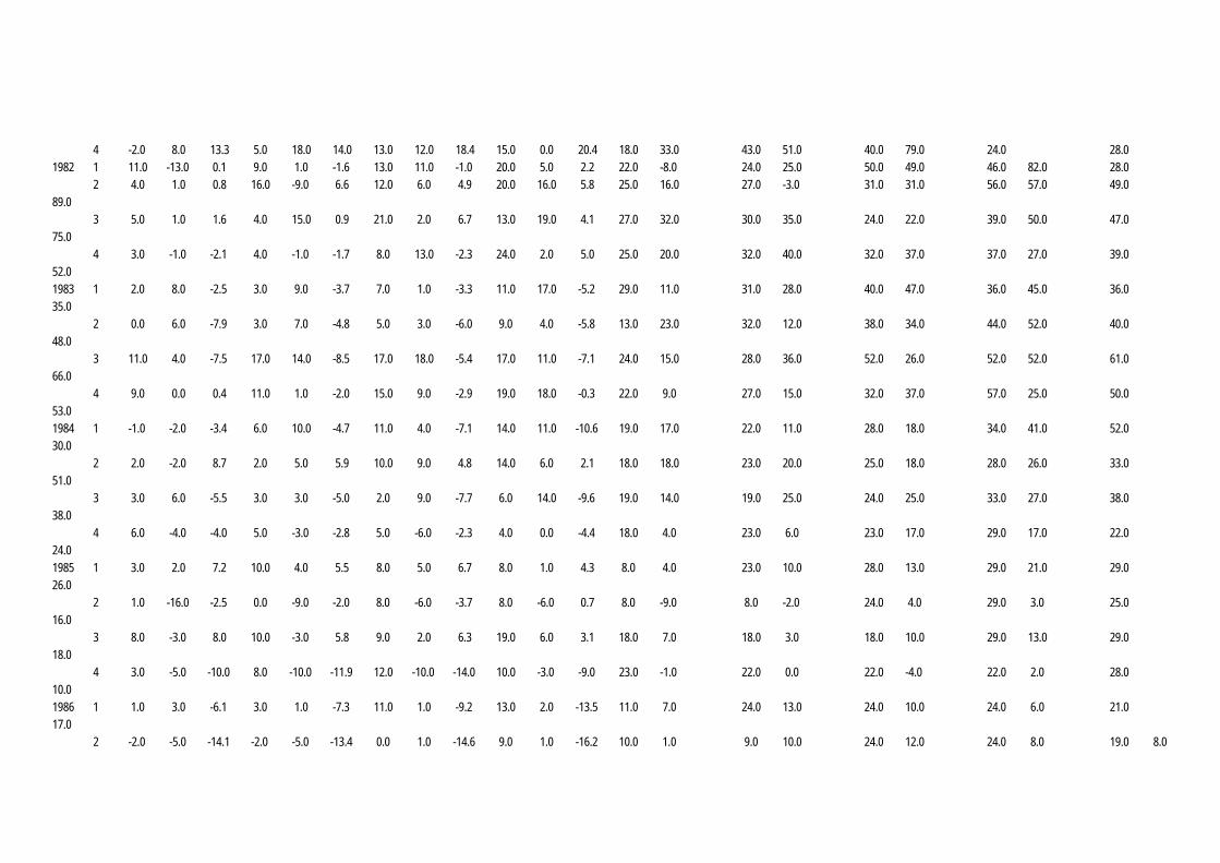
Table 1 summarises the non-parametric analysis of the TPI

forecast produced by BCIS between 1980:2 and 1990:4 for 0, 1,

..., 8 quarter forecast horizons in terms of mean error, mean

absolute error, mean percentage error, RMSE, RMSE (percent) and

Theil U2. The standard deviations of the mean error, mean

absolute error and mean percentage error are given to indicate

the spread of these measures. All the measures of forecasting

accuracy indicate a decrease in the accuracy of the forecast as

the horizon of the forecast increases. The increase in standard

deviation of ME, MEA and MPE as the horizon increases indicates

an increase in uncertainty concerning future economic events.

The forecast of TPI is positively biased, indicating a general

over-estimation of TPI during this period as might be expected

in these times of generally increasing building activity. The

forecasts of TPI made between 1980:2 and 1981:1 were clearly

high. A possible explanation for this is that this was a

learning period for BCIS 'experts', as it coincided with the

13

time when TPI forecasts were formally published for the first

time.

Error decomposition

Decomposition of the mean square error of the TPI forecasts

(after Theil, 1966) is shown in Table 2. These statistics are

useful in identifying sources of TPI forecast error and thus

offer the possibility of future correction or improvement in the

TPI forecast.

Using Theil's first method of error decomposition, the values of

the components show that the covariance proportion UC accounts

for a greater proportion of the MSE of the level of forecasts

than the bias, UM, and variance proportion, US. As the forecast

horizon increases, UC decreases while UM increases, confirming

the existence of a direct relationship between forecast horizon

and over-estimation.

The second error decomposition method indicates that nearly all

the MSE of the TPI forecasts is attributable to the regression

proportion UR. The F-statistics are significant at 5 percent

confidence level (p=0.000 in all cases). This produces evidence

that the forecasters made errors of a systematic nature and

produced statistical grounds to support the hypothesis that a =

0 and b = 1. This being the case, the MSE of the forecast could

14

be reduced using an optimal linear correction technique. The

resulting estimated coefficients for each of the forecast

horizons could be used as correction factors thus:

Where

At = Corrected forecast value

P = Predicted value

The regression proportion decreases with the forecast horizon

which shows that the degree to which the MSE of TPI forecast

could be reduced, decreases with increasing forecast horizon.

THE DL&E SYSTEM

Davis, Langdon and Everest (DL&E) is a private firm of chartered

quantity surveyors and a profit making organisation, formerly

known as Davis Belfield and Everest (DB&E) and Langdon and Every

(L&E) until the end of 1987. DL&E has been involved in

monitoring building prices since the early 1970s, though its

first historical index and predictive index (forecast) of tender

price was not published until 12 November 1975. This was

published in Architects' Journal under the caption "technical

study". In the 7th forecast feature (Architects' Journal, 26

October, 1977) of DB&E the caption was changed to "Building

15

Costs". In November 1982, the caption was changed again to

"COST FORECAST". The Architects' Journal continued to publish

the quarterly edition of the cost information from DL&E until 5

July 1989. DL&E resumed publication of tender price level

information in the Building magazine with the caption "COST

FORECAST" in October, 1989.

The DL&E tender price index reflects changes in the level of

pricing in bills of quantities for accepted tenders in the outer

London area. The forecast of TPI produced and published by DL&E

is of the prediction interval form.

16

Forecasting system2

DL&E do not have a formal model for tender price forecasting.

The forecast of TPI is based on "subjective assessment of in-

house experts". The forecasting method being adopted by this

organisation could best be described as qualitative or Delphic.

Experts within the organisation confer to analyze the current

economic climate and how this will affect the future prices of

construction.

An important leading factor considered by the experts in

forecasting tender price movements is the level of architects'

appointments. The architects appointments advertisements are

measured by determining the total area covered by advertisement

for architects in Architects' Journal. The organisation has

derived a lagged relationship between the architect appointment

advertisement and market factor over time. Figs 4 and 5 show

the annual and quarterly graphical illustrations, respectively,

of correlation established by DL&E between the two variables.

Normally, the 'Market Factor Index' provides a measure of how

tender prices relate to building costs thus:

Tender Price Index (TPI) Market factor index (MFI) = ----------------------- Building Cost Index (BCI)

2 The information in this section was obtained directly from DL&E (Smith and Fordham, 1981).

17

However, the 'Market Factor Index' is pre-determined using the

architects' appointment advertisement. Also the DL&E system is

capable of forecasting the Building Cost Index with a high

degree of accuracy. Having established these two indexes, a

tentative tender price index forecast is calculated thus:

TPI = MFI x BCI

Considering the tentative TPI prediction and other factors

(financial, non-financial and prices) the 'experts' are able to

arrive at the minimum and maximum tender price index forecasts

for 0, 1, ..., 8 quarter forecast horizons.

However, this organisation considers that the building cost

trend has little influence on the judgemental adjustments to the

tender price index forecast. The most important factor,

considered to have a major impact on DL&E forecasts of TPI,

relates to market conditions and this predominantly includes

interest rates, business confidence, general retail inflation

and construction new orders.

18

DL&E monitors the accuracy of its published forecasts and is

confident that its judgemental forecasting system is more

accurate than those of a purely quantitative nature. The main

difficulties in forecasting TPI, that they have identified, are

in the accurate prediction of the timing of turning points in

TPI and obtaining accurate forecasts of the general level of

retail inflation beyond a two year time horizon.

Forecast accuracy

The forecast accuracy of the DL&E TPI was investigated, again

using both graphical presentation and non-parametric tests of

accuracy. The forecast period in this case covered the fifteen

years between 1975:4 and 1990:4 for 0, 1, ..., 8 quarter

forecast horizons. This provided 61 zero-quarters-ahead

forecasts, 60 one-quarter-ahead forecasts, 59 two-quarter-ahead

forecasts, ..., 53 eight-quarter-ahead forecasts.

Graphical presentation

19

Fig 6 presents the plots of actual and predicted values of the

tender price index. The predictions show the minimum and

maximum values. The plots presented in the figure relate to

values (actual, minimum prediction and maximum prediction)

between 1978:1 and 1990:4 to allow a standardized comparison of

performances across forecast horizons. The plots of the

predicted values cover the eight-quarter forecast horizon. The

plots present a clear picture of the performance of the DL&E

forecasts of the TPI.

Visual observation of these plots shows that the TPI forecasts

generally track the actual levels closely up to the two quarter

horizon. As DL&E make prediction interval forecasts, the actual

values of TPI are expected to fall within the minimum and

maximum predicted values in most cases. This was not so,

however, for all two quarter and above forecast horizons, the

actual values of TPI were either below the minimum predicted

values or above the maximum predicted values. The disparity

between actual and predicted values noticeably increases with

increasing forecast horizons. The turning points in the

predicted values occur about 2 to 4 quarters after the turning

points in the actual values - an indication perhaps of the

postmortem judgemental adjustment strategy in the DL&E forecast.

Non-parametric analysis

20

The predicted values of the TPI comprise the minimum and the

maximum values only. In the absence of any other information,

it is assumed that these values are intended to represent the

limits of some symmetrical probability distribution of possible

values. It can be shown that the best estimate of the expected

value of such a distribution is the arithmetic mean of these

maximum and minimum values. As the expected value of the

forecast has an equal probability of being too high or too low,

it is reasonable to assume, that this can be used to estimate

the value of DL&E's absent point forecast of TPI.

Table 1 includes the results of the non-parametric analysis of

the DL&E TPI estimated point forecasts between 1976:4 and 1990:4

for 0, 1, ..., 8 quarter forecast horizons. The non-parametric

measures of forecasting accuracy employed are ME, MAE, and MPE

with their respective standard deviations; RMSE, RMSE (percent)

and Theil U2. All the measures of forecasting accuracy point to

a decrease in the accuracy of the estimated point forecasts as

the horizon of the forecasts increases. The estimated point

forecasts are generally positively biased, indicating a general

over-estimation of the TPI.

COMPARISON BETWEEN THE BCIS AND THE DL&E SYSTEMS

The BCIS and DL&E are both involved in monitoring and

21

forecasting TPIs. The tenders included in the compilation of

the indexes published by these two organisations are drawn from

both the public and the private sector. However, there are some

differences associated with the monitoring and forecasting of

the TPIs by these two organisations, thus:

1. the BCIS series indexes the price levels of new building

work in the UK whilst the DL&E series indexes the price

levels of new building work in the outer London area.

2. the BCIS base year is 1974 while the DL&E base year is

1976.

3. the BCIS provide point forecasts whilst DL&E provide

prediction-interval forecasts.

4. the BCIS commenced publication of its TPI forecast in 1980

whilst DL&E commenced in 1976.

Despite these differences, there are few problems in comparing

the accuracy of the TPI forecasts. Both TPIs index the same

phenomenon, building price movements, and both are constructed

in essentially the same manner. As would be expected, the

indexes are highly correlated (r2=0.970, n=68) and the impact of

the small differences that do occur between the indexes can be

lessened by the use of percentage rather than absolute error

measures.

22

Comparative performance analyses were made, covering the entire

period over which these two organisations published TPI

forecasts (BCIS, 1980-1990; DL&E, 1976-1990), so that a period

of learning could be equally included in the analysis. Table 1

gives the non-parametric summary analysis of the forecasting

accuracy. Two measures of accuracy enable a direct comparison

to be made between these two forecasts apart from graphical

representation: RMSE(%) and Theil U2. Although the DL&E's

estimated point forecast at zero-quarter horizon performed

better than the BCIS's, RMSE(%) and Theil U2 show that the BCIS

forecast of TPI was more accurate than DL&E estimated point

forecast at all other forecast horizons over the time period

examined.

Two other points also emerge from this analysis:

1. The forecast accuracy of these organisations has varied

greatly over time. For example, whilst the BCIS were able

to make relatively accurate forecasts between 1985:1 and

1987:4, this has not been the case in other periods. One

possible explanation of this is that the period between

1985:1 and 1987:4 coincided with a steady growth in UK

economic conditions, and that the reduced level of

uncertainty associated with this period provided conducive

conditions for more accurate economic forecasting. An

unexpected decline in economic fortunes would therefore be

23

associated with a greater level of uncertainty and would

lead to less accurate forecasts.

2. Fluctuations in forecast accuracy over this period could be

attributable to the 'expert' forecasters. Different people

have been involved in forecasting TPI values within these

organisations (Martin, 1991; Smith and Fordham, 1991).

These fluctuations in accuracy could therefore be

attributable to lack of continuity and/or systematic

differences in forecasting skills of the 'experts'

involved.

A&S REDUCED-FORM EQUATION

In a recent paper, Akintoye & Skitmore (1993) described the

development of models based on single structural and

simultaneous equation techniques to explain the movements in

macro building prices over the years 1974 to 1987. A reduced

form simultaneous equation model was used to explain general

movements, and a single structural model, based on economic

theory, to explain structural movements in the TPI. Both models

were found to fit the BCIS TPI well. Single structural models

however are known to have an inferior predictive power to

reduced-form equations (Kane, 1968:21-2; Neal and Shone, 1976)

and therefore only the reduced-form equation is considered here.

24

This section examines the forecasting accuracy of the A&S

reduced form model over different horizon lengths. It also

determines if the model will display a tendency to accumulate

errors as the forecasting horizon increases. As a result of

data limitations, the three quarter time horizon is the maximum

used.

A&S Reduced-form model

Akintoye and Skitmore's (1993) reduced-form model of

construction price is a causal quantitative forecasting model

involving the identification of variables that are related to

construction price. The model is derived from the construction

demand, supply and equilibrium equations for the period 1974 to

1987 as follows:

Demand equation Qdt = -14.051 - 0.766Pt-3 - 0.249UEt-5 +

1.764Mpt-4 - 0.011Rrt-1 + 1.632Yd

Supply equation Qst = 1.049 + 0.970Pt + 0.628Prt-4 - 0.695Cpt-2

- 0.019STt-3 + 0.239Frt-8 - 0.093OLt-1

Equilibrium equation Qst = 3.281 + 0.197Qdt + 0.158Qdt-1 +

25

0.106Qdt-2 + 0.055Qdt-3 + 0.02Qdt-4

+ 0.016Qdt-5 + 0.058Qdt-6

where

Qd Quarterly construction new orders

Qs Quarterly construction output

PQuarterly Tender Price Index.

Pr Output per person employed in the construction industry.

Cp Quarterly Building Cost Index.

ST The working days lost by workers both directly or

indirectly involved in operation of construction industry

due to industrial disputes.

Fr Number of registered private contractors.

OL Dummy variable to reflect general increase in prices

between 1978 and 1980 due to oil crisis (During this

period of oil shock, the real price of crude oil went

up by 110 percent): equal 1 between 1978:2 and 1980:2

and zero otherwise.

Ue Number claiming unemployment-related benefit at

Unemployment Benefit Offices.

Mp Manufacturing output price/input cost ratio.

Rr Real rate of interest.

Yd Quarterly gross national product.

26

P (tender price level) in these equations is therefore an

endogenous variable. These equations are solved simultaneously

for P by substituting the demand equation into the equilibrium

equation and letting this equal the supply equation, giving P = -6.424 - 0.647Prt-4 + 0.716Cpt-2 + 0.0196STt-3 - 0.246Frt-8 + 0.096OLt-1 - (0.155Pt-3 + 0.125Pt-4 + 0.083Pt-5 + 0.043Pt-6 + 0.015Pt-7 + 0.012Pt-8 + 0.046Pt-9) - (0.050UEt-4 + 0.041UEt-5 + 0.027UEt-6 + 0.014UEt-7 + 0.005UEt-8 + 0.004UEt-9 + 0.015UEt-10) + (0.357Mpt-4 + 0.287Mpt-5 + 0.192Mpt-6 + 0.099Mpt-7 + 0.035Mpt-8 + 0.028Mpt-9 + 0.105Mpt-10) - (0.002Rrt-1 + 0.002Rrt-2 + 0.001Rrt-3 + 0.0006Rrt-4 + 0.0002Rrt-5 + 0.0002Rrt-6 + 0.0006Rrt-7) + (0.331Yd + 0.266Ydt-1 + 0.178Ydt-2 + 0.091Ydt-3 + 0.032Ydt-4 + 0.026Ydt-5 + 0.097Ydt-6) (20)

This reduced-form model readily produces forecasts of TPI at

zero-quarter horizon. However, it can also be manipulated to

produce the forecast of TPI up to three quarters horizon.

Cp, Yd and Rr in the reduced-form model have the starting lagged

distribution of 0, 0, and 1 respectively which suggests that

these concurrent relationships have little forecasting value.

Also, the starting point of distributed lags for the remaining

variables is a three or more quarters lead, which does not pose

forecasting problems. There are three options for dealing with

the concurrent relationship variables in the model:

1. Forecasts of these concurrent independent variables for the

relevant period could be used where available, provided the

forecasts are very accurately predicted. An example in

27

this respect is Cp (Building Cost Index), which is known to

have a high degree of accuracy (Fellows, 1988).

2. These variables could be simulated provided they have

either a fairly steady growth, decay or zero trend. A

problem does arise however when the trends in exploratory

variables fluctuate markedly. Such trends in economic

variables may be associated with and/or lead to slump

(recession) or boom (recovery) in the economy. This is

always a problem in economic forecasts and may result in

large errors (McNees and Rees, 1983).

3. The current values of these variables could be lagged 3, 2,

or 1 quarter ahead of TPI depending on the forecast span

(horizon) intended. Fig 7 provides an illustration of how

the current value of Yd for example, could be used in

predicting TPI up to a three quarters horizon. As the

latest values of the variable become available, the

forecast is revised to fit the new information (after

McNees, 1986).

Here we adopt options 1 and 3 for forecasting purposes. It

should be noted that the in-sample and post-sample forecasts

analysed are purely mechanically-generated reduced-form model

based forecasts. No 'expert' opinion or delphic-like adjustment

has been made.

28

Non-parametric analysis

Ex post simulation or "historical" simulation forecast accuracy

The simultaneous equation estimation was based on quarterly data

from 1974:1 to 1987:4. This period is regarded, therefore, as

the in-sample period. The in-sample non-parametric forecast

accuracy of the A&S model of construction price is shown in

Table 1. The RMSE is less than 10 in all cases. The percentage

error of less than 5 percent across the forecast horizon

indicates that the model as a whole does not display any

substantial tendency to accumulate errors as the forecasting

horizon lengthens. Though the MPE and ME statistics show

negative signs, their standard deviations (spread) indicate an

almost equal tendency of the model towards under-prediction and

over-prediction.

Ex post forecast accuracy

1988:1 to 1990:4 is the ex-post or out-sample period. Co-

incidentally, this period is of special interest because it has

witnessed a significant downturn in the tender price level,

coupled with a severe economic recession. The non-parametric

forecast accuracy of the A&S model of construction price was

compared with the accuracy of the BCIS forecasts and DL&E

29

estimated point forecasts over the same period. Table 3

contains error statistics for the forecasts. The table

indicates, interestingly, that the post-sample error statistics

for the A&S model are not significantly larger than its in-

sample error statistics. The table also shows that the A&S

model has a better predictive behaviour than the BCIS forecasts

and the DL&E estimated point forecasts. RMSE (percent) of the

A&S model forecasts is less than 6 percent in all cases over the

three-quarter forecast horizon. The A&S model, however,

generally underestimated the TPI values compared to a general

overestimation of the BCIS forecasts and the DL&E estimated

point forecasts.

Graphical presentation

Fig 8, which shows the graphical plots of actual values of TPI

and the predicted values from 1976 through 1990, presents a

clear picture of the performance of the A&S model in tracking

the historical record.

30

Ex post simulation - within sample

The period 1976:2 to 1987:4 represents the in-sample period. As

expected, the model simulates the historical record quite well

particularly over the zero-quarter and one-quarter forecast

horizon. The figure shows the results for 0, 1, 2, 3 quarter

forecast horizons indicating that the A&S model can predict the

turning point in the TPI movements not later than a quarter

thereafter.

Ex post forecast - post sample

1988:1 to 1990:4 is the out-sample or ex post forecast period.

The magnitude and direction of the forecasting errors are

illustrated by the plot over the three-quarter forecast horizon.

The visual disparity between actual values and predicted values

during the ex post forecast period is not as pronounced as in

the BCIS forecasts and the DL&E estimated point forecasts.

The over-prediction of the model from 1989:4 is probably due to

the continuous severity of the recession. The model does seem

to anticipate the recession through its impact on GNP, the

unemployment level and interest rate. However, there are other

factors associated with the recession that are not anticipated.

Clearly, the suddenness of the current recession was not

anticipated by any of the systems.

31

COMPARISON BETWEEN BCIS, DL&E AND A&S SYSTEMS

Table 1 compares the forecast accuracy of these systems has

varied over different forecast horizons and forecast periods.

The periods 1979:2 to 1981:2, 1984:3 to 1986:1 and 1989:1 to

date are associated with recessions in the UK. The largest

forecast errors occurred during these recessionary periods and

increased with the length of time span (forecast horizon). This

is not unusual in economic forecasts (McNees and Ries, 1983)

particularly in a changing economy. Longer time spans involve

larger changes for most economic variables and this is reflected

in the larger errors as the time span increases.

A valid comparison of different forecasts requires that the

forecasts are examined over the same forecast horizon and

period. The A&S system is capable of forecasting TPI up to a

three quarter horizon in its present form and hence may be

compared with the BCIS and DL&E systems over the same forecast

horizon. The BCIS and DL&E systems have different forecast

periods due to different commencements of publication. To

ensure that the learning period of these two systems are taken

into consideration, all the periods of the forecast of these

systems are compared with the A&S system in-sample forecasts

(Table 1). The reliability of the A&S system is examined by

comparing the A&S out-sample forecasts with the BCIS and DL&E

32

forecasts over the same period.

Figs 9 and 10 compares the BCIS and DL&E forecast accuracy with

the A&S in-sample and out-sample forecast accuracy respectively.

These comparisons show that the A&S system generally produces

better in-sample and out-sample forecasts than BCIS and DL&E

with the exception of in-sample forecasts for the zero quarter

forecast horizon.

SUMMARY AND CONCLUSION

This paper analyses the accuracy of TPI forecasts produced and

published by Building Cost Information Service between 1980 and

1990 and Davis Langdon and Everest forecasts between 1976 and

1990. The disparities between the actual values of TPI and the

predicted values published by these organisations increased with

increasing forecast horizon.

Comparisons were made between the actual forecasts published by

the Building Cost Information Service and the estimated point

forecasts of Davis, Langdon & Everest and simulated out-sample

forecasts made by the Akintoye and Skitmore system over the

years 1988 to 1990. It is shown that the Akintoye and Skitmore

system gives the most accurate forecasts for a zero to three

quarters forecast horizon for which it is capable of producing

33

forecasts in its present form.

Two points are worthy of note concerning this analysis.

Firstly, only the static form of the Akintoye and Skitmore

system is examined here. The coefficients of the model were

estimated once only, at the end of 1987. Clearly we would

expect these estimates to deteriorate over time so that using

the 1987 model in 1989 to make forecasts for 1990 is not likely

to be as good as using a 1989 calibrated model to make forecasts

for 1990. In other words, we would expect a dynamic version of

this system, taking into account all the data available at the

time of forecast, to produce more accurate forecasts than the

static version examined here.

Secondly, the forecasts produced by the A&S model are purely

mechanically-generated. It is possible that the accuracy of

forecasts based on the A&S model could be improved further if

used as a forecasting tool by experts. In this respect, experts

would be expected to be capable of making "objective"

judgemental adjustments of the mechanically-generated model-

based forecasts. Such adjustments are a common feature of

forecasting systems of these kind, including the BCIS and DL&E

systems examined here. Whether human interference will really

be beneficial is clearly an empirical matter yet to be studied.

The major issues have however been suggested in this paper and

these concern the abilities and experience of the 'expert' both

in price forecasting generally and in coping with rapidly

34

changing economic circumstances.

Finally, it should be emphasised that the time period studied

was of special interest, in that it contained a significant

downturn in tender price levels together with a severe economic

recession. Whilst the analysis of this period has shed some

light on forecasting behaviour under such conditions, it is not

easy to generalise these findings to other economic

circumstances. Indeed, it is not inconceivable that the very

process of publishing these results may influence the future

behaviour of forecasters in an unpredictable way.

ACKNOWLEDGEMENTS

The authors would like to thank David and Karen Eaton, the two

anonymous reviewers and the editors for their kind and helpful

comments in the preparation of the final version of this

paper.the two anonymous reviewers for their very useful and

extensive guidance in the preparation of the final version of

this paper.

REFERENCES

Akintoye, A.S., Skitmore, R.M., 1993, Macro models of UK

construction prices, Civil Engineering Systems (in print).

35

BCIS, 1974-90, Statistics and economic indicators, Sub-section

AG.

BCIS, 1987, BCIS - A policy statement, BCIS NEWS, March, No.13

Bowerman, B.L., O'Connel, R.T., 1987, Time series forecasting,

Boston, Duxbury Press.

Dhrymes, P.J., Howrey, E.P., Hymans, S.H., Kmenta, J., Leamer,

E.E., Quandt, R.E., Ramsey, H.T., Shapiro, H.T., Zarnowitz, V.,

1972, Criteria for evaluation of econometric models, Annals of

Economics and Social Measurement, 1(3), 291-324.

Evans, M.K., Haitovsky, Y., Treyz, G.I., 1972, An analysis of

the forecasting properties of U.S economic models, in

Econometric Models of Cyclical Behaviour, B.G. Hickman, ed.,

National Bureau of Economic Research, Studies in Income and

Wealth, No.36, New York, NBER, 949-1139.

Fellows, R.F., 1988, Escalation management, PhD thesis,

Department of Construction Management, University of Reading.

Haitovsky, Y., Treyz, G.I., 1972, Forecasts with quarterly

macroeconomic models, equation adjustments and benchmark

predictions: The U.S. experience, Review of Economics and

Statistics, 54, Aug, 317-25.

36

Holden, K., Peel, D.A., 1988, A comparison of some inflation,

growth and unemployment forecast, Journal of Economic Studies,

15(5), 45-52.

Kahneman, D., Tversky, A., 1982, Intuitive prediction: Biases

and corrective procedures, in Judgement Under Uncertainty:

Heuristics and Biases, Kahneman, Slovic and Tversky, eds.,

Cambridge University Press, New York, 414-21.

Kane, E.J., 1968, Economic statistics and econometrics: an

introduction to quantitative economics, Harper and Row, London.

Lucas, R.E. Jr., 1976, Economic policy evaluation, a critique,

in The Phillips Curve and Labour Markets, K. Brunner and A.H.

Meltzler, eds., Carnegie-Rochester Conference on Public Policy,

1.

McCaffer, R., McCaffrey, M.J., Thorpe, A., 1983, The disparity

between construction cost and tender price movements,

Construction papers, 2(2), 17-27.

McNees, S.K., 1985, Which forecast should you use?, New England

Economic Review, Jul/Aug, 36-42.

McNees, S.K., 1986, Estimating GNP: the trade-off between

timeliness and accuracy, New England Economic Review, Jan/Feb,

37

3-10.

McNees, S.K., 1989, Why do forecast differs, New England

Economic Review, Jan/Feb, 42-54.

McNees, S.K., 1990, Man Vs Models? The role of judgement in

forecasting, New England Economic Review, Jul/Aug, 41-52.

McNees, S.K., Ries, J., 1983, The track record of macroeconomic

forecasts, New England Economic Review, Nov/Dec, 5-18.

Makridakis, S., 1984, Forecasting: state of the art, in The

forecasting accuracy of major time series methods, Makridakis, S

et al, John Wiley & Sons, New York, 1-17.

Makridakis, S., Hibon, M., 1984, Accuracy of forecasting: an

empirical investigation, in The Forecasting Accuracy of Major

Time Series Methods, Makridakis, S, et al, John Wiley & Sons,

New York, 35-59.

Martin, J.L.N., 1991, Personal communication.

Neal, F., Shone, R., 1976, Economic model building, McMillan,

London.

O'Donovan, T.M., 1983, Short term forecasting: an introduction

to the Box-Jenkins approach, John Wiley & Sons, New York, 5-7.

38

Pindyck, R.S., Rubinfeld, D.L., 1976, Econometric models and

economic forecasts, McGraw-Hill, New York.

Sim, C.A., 1980, Macroeconomics and Reality, Econometrica, 48,

Jan, 1-48.

Skitmore, M., Stradling, S., Tuohy, A., Mkwenzalamba, H., 1990,

Accuracy of construction price forecasts, The University of

Salford, Salford, UK.

Smith, R., Fordham, P., 1991, Personal communication.

Theil, 1966, Applied economic forecasting, North Holland

Publishing Company, Amsterdam.

Trehan, B., 1989, Forecasting growth in current quarter real

GNP, Economic Review, Federal Reserve Bank of San Francisco,

Winter, pp. 39-51.

Zarnowitz, V., 1979, An analysis of annual and multiperiod

quarterly forecast of aggregate income, output and price level,

Journal of Business, 52(1), Jan, 24-38.

39

FIGURES AND TABLES List of Captions Figures Fig 1: Types of economic forecast Source: Pindyck & Rubinfeld (1976:313). Fig 2: Actual and predicted tender price index Source: Building Cost Information Service 24-month index

forecast Fig 3: Frequency distribution of forecast mean percentage error Fig 4: Relationship between Architects' appointments advertised in Architects Journal and DL&E Market Factor (based on first quarter each year) Source: Davis, Langdon and Everest. Fig 5: Relationship between Architects' appointments advertised in Architects Journal and DL&E Market Factor (on quarterly basis) Source: Davis, Langdon and Everest. Fig 6: Actual and Predicted Tender Price Index Source: Davis, Langdon and Everest. Fig 7: Lag relationship between P and Yd Fig 8: Actual and predicted Tender Price Index, A&S Reduced-form model of construction price. Fig 8 (contd): Actual and predicted Tender Price Index, A&S Reduced-form model of construction price. Tables Table 1: Comparative analysis of forecasting accuracy of the A&S Model forecast, BCIS forecast and DL&E estimated point forecast (1975:4 - 1990:4) Table 2: Decomposition of Mean Squared Error (MSE) of TPI forecast Table 3: Comparative analysis of forecasting accuracy of the A&S Model forecast, BCIS forecast and DL&E estimated point forecast (1988:1 - 1990:4)

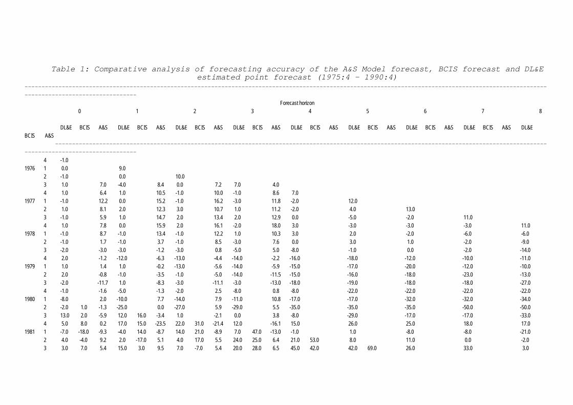
Table 1: Comparative analysis of forecasting accuracy of the A&S Model forecast, BCIS forecast and DL&E estimated point forecast (1975:4 - 1990:4) ------------------------------------------------------------------------------------------------------------------------------------------------------------------------------------------- Forecast horizon 0 1 2 3 4 5 6 7 8 DL&E BCIS A&S DL&E BCIS A&S DL&E BCIS A&S DL&E BCIS A&S DL&E BCIS A&S DL&E BCIS A&S DL&E BCIS A&S DL&E BCIS A&S DL&E BCIS A&S ---------------------------------------------------------------------------------------------------------------------------------------------------------------------------------- 4 -1.0 1976 1 0.0 9.0 2 -1.0 0.0 10.0 3 1.0 7.0 -4.0 8.4 0.0 7.2 7.0 4.0 4 1.0 6.4 1.0 10.5 -1.0 10.0 -1.0 8.6 7.0 1977 1 -1.0 12.2 0.0 15.2 -1.0 16.2 -3.0 11.8 -2.0 12.0 2 1.0 8.1 2.0 12.3 3.0 10.7 1.0 11.2 -2.0 4.0 13.0 3 -1.0 5.9 1.0 14.7 2.0 13.4 2.0 12.9 0.0 -5.0 -2.0 11.0 4 1.0 7.8 0.0 15.9 2.0 16.1 -2.0 18.0 3.0 -3.0 -3.0 -3.0 11.0 1978 1 -1.0 8.7 -1.0 13.4 -1.0 12.2 1.0 10.3 3.0 2.0 -2.0 -6.0 -6.0 2 -1.0 1.7 -1.0 3.7 -1.0 8.5 -3.0 7.6 0.0 3.0 1.0 -2.0 -9.0 3 -2.0 -3.0 -3.0 -1.2 -3.0 0.8 -5.0 5.0 -8.0 -1.0 0.0 -2.0 -14.0 4 2.0 -1.2 -12.0 -6.3 -13.0 -4.4 -14.0 -2.2 -16.0 -18.0 -12.0 -10.0 -11.0 1979 1 1.0 1.4 1.0 -0.2 -13.0 -5.6 -14.0 -5.9 -15.0 -17.0 -20.0 -12.0 -10.0 2 2.0 -0.8 -1.0 -3.5 -1.0 -5.0 -14.0 -11.5 -15.0 -16.0 -18.0 -23.0 -13.0 3 -2.0 -11.7 1.0 -8.3 -3.0 -11.1 -3.0 -13.0 -18.0 -19.0 -18.0 -18.0 -27.0 4 -1.0 -1.6 -5.0 -1.3 -2.0 2.5 -8.0 0.8 -8.0 -22.0 -22.0 -22.0 -22.0 1980 1 -8.0 2.0 -10.0 7.7 -14.0 7.9 -11.0 10.8 -17.0 -17.0 -32.0 -32.0 -34.0 2 -2.0 1.0 -1.3 -25.0 0.0 -27.0 5.9 -29.0 5.5 -35.0 -35.0 -35.0 -50.0 -50.0 3 13.0 2.0 -5.9 12.0 16.0 -3.4 1.0 -2.1 0.0 3.8 -8.0 -29.0 -17.0 -17.0 -33.0 4 5.0 8.0 0.2 17.0 15.0 -23.5 22.0 31.0 -21.4 12.0 -16.1 15.0 26.0 25.0 18.0 17.0 1981 1 -7.0 -18.0 -9.3 -4.0 14.0 -8.7 14.0 21.0 -8.9 7.0 47.0 -13.0 -1.0 1.0 -8.0 -8.0 -21.0 2 4.0 -4.0 9.2 2.0 -17.0 5.1 4.0 17.0 5.5 24.0 25.0 6.4 21.0 53.0 8.0 11.0 0.0 -2.0 3 3.0 7.0 5.4 15.0 3.0 9.5 7.0 -7.0 5.4 20.0 28.0 6.5 45.0 42.0 42.0 69.0 26.0 33.0 3.0

4 -2.0 8.0 13.3 5.0 18.0 14.0 13.0 12.0 18.4 15.0 0.0 20.4 18.0 33.0 43.0 51.0 40.0 79.0 24.0 28.0 1982 1 11.0 -13.0 0.1 9.0 1.0 -1.6 13.0 11.0 -1.0 20.0 5.0 2.2 22.0 -8.0 24.0 25.0 50.0 49.0 46.0 82.0 28.0 2 4.0 1.0 0.8 16.0 -9.0 6.6 12.0 6.0 4.9 20.0 16.0 5.8 25.0 16.0 27.0 -3.0 31.0 31.0 56.0 57.0 49.0 89.0 3 5.0 1.0 1.6 4.0 15.0 0.9 21.0 2.0 6.7 13.0 19.0 4.1 27.0 32.0 30.0 35.0 24.0 22.0 39.0 50.0 47.0 75.0 4 3.0 -1.0 -2.1 4.0 -1.0 -1.7 8.0 13.0 -2.3 24.0 2.0 5.0 25.0 20.0 32.0 40.0 32.0 37.0 37.0 27.0 39.0 52.0 1983 1 2.0 8.0 -2.5 3.0 9.0 -3.7 7.0 1.0 -3.3 11.0 17.0 -5.2 29.0 11.0 31.0 28.0 40.0 47.0 36.0 45.0 36.0 35.0 2 0.0 6.0 -7.9 3.0 7.0 -4.8 5.0 3.0 -6.0 9.0 4.0 -5.8 13.0 23.0 32.0 12.0 38.0 34.0 44.0 52.0 40.0 48.0 3 11.0 4.0 -7.5 17.0 14.0 -8.5 17.0 18.0 -5.4 17.0 11.0 -7.1 24.0 15.0 28.0 36.0 52.0 26.0 52.0 52.0 61.0 66.0 4 9.0 0.0 0.4 11.0 1.0 -2.0 15.0 9.0 -2.9 19.0 18.0 -0.3 22.0 9.0 27.0 15.0 32.0 37.0 57.0 25.0 50.0 53.0 1984 1 -1.0 -2.0 -3.4 6.0 10.0 -4.7 11.0 4.0 -7.1 14.0 11.0 -10.6 19.0 17.0 22.0 11.0 28.0 18.0 34.0 41.0 52.0 30.0 2 2.0 -2.0 8.7 2.0 5.0 5.9 10.0 9.0 4.8 14.0 6.0 2.1 18.0 18.0 23.0 20.0 25.0 18.0 28.0 26.0 33.0 51.0 3 3.0 6.0 -5.5 3.0 3.0 -5.0 2.0 9.0 -7.7 6.0 14.0 -9.6 19.0 14.0 19.0 25.0 24.0 25.0 33.0 27.0 38.0 38.0 4 6.0 -4.0 -4.0 5.0 -3.0 -2.8 5.0 -6.0 -2.3 4.0 0.0 -4.4 18.0 4.0 23.0 6.0 23.0 17.0 29.0 17.0 22.0 24.0 1985 1 3.0 2.0 7.2 10.0 4.0 5.5 8.0 5.0 6.7 8.0 1.0 4.3 8.0 4.0 23.0 10.0 28.0 13.0 29.0 21.0 29.0 26.0 2 1.0 -16.0 -2.5 0.0 -9.0 -2.0 8.0 -6.0 -3.7 8.0 -6.0 0.7 8.0 -9.0 8.0 -2.0 24.0 4.0 29.0 3.0 25.0 16.0 3 8.0 -3.0 8.0 10.0 -3.0 5.8 9.0 2.0 6.3 19.0 6.0 3.1 18.0 7.0 18.0 3.0 18.0 10.0 29.0 13.0 29.0 18.0 4 3.0 -5.0 -10.0 8.0 -10.0 -11.9 12.0 -10.0 -14.0 10.0 -3.0 -9.0 23.0 -1.0 22.0 0.0 22.0 -4.0 22.0 2.0 28.0 10.0 1986 1 1.0 3.0 -6.1 3.0 1.0 -7.3 11.0 1.0 -9.2 13.0 2.0 -13.5 11.0 7.0 24.0 13.0 24.0 10.0 24.0 6.0 21.0 17.0 2 -2.0 -5.0 -14.1 -2.0 -5.0 -13.4 0.0 1.0 -14.6 9.0 1.0 -16.2 10.0 1.0 9.0 10.0 24.0 12.0 24.0 8.0 19.0 8.0

3 -1.0 -10.0 -14.9 -3.0 -2.0 -18.0 -2.0 -1.0 -17.2 -2.0 1.0 -18.2 9.0 2.0 12.0 2.0 10.0 9.0 26.0 14.0 26.0 14.0 4 5.0 -3.0 -11.5 1.0 -3.0 -8.7 0.0 2.0 -11.8 0.0 4.0 -10.3 4.0 8.0 11.0 10.0 13.0 9.0 13.0 16.0 29.0 19.0 1987 1 -5.0 3.0 -1.1 0.0 -10.0 -7.3 -6.0 -10.0 -4.2 -7.0 -5.0 -11.3 -7.0 -1.0 -1.0 0.0 6.0 2.0 8.0 2.0 7.0 7.0 2 -2.0 8.0 -6.4 -10.0 12.0 -9.4 -3.0 -3.0 -15.2 -8.0 -3.0 -11.6 -12.0 0.0 -11.0 6.0 -6.0 8.0 0.0 11.0 2.0 10.0 3 -8.0 10.0 9.8 -9.0 9.0 5.3 -17.0 14.0 2.1 -10.0 -1.0 -3.1 -15.0 -1.0 -18.0 7.0 -18.0 13.0 -17.0 15.0 -5.0 17.0 4 -4.0 -9.0 -8.7 -15.0 -8.0 -11.1 -20.0 -9.0 -15.6 -28.0 -2.0 -17.7 -22.0 -17.0 -27.0 -16.0 -29.0 -9.0 -30.0 -7.0 -26.0 -3.0 1988 1 1.0 -13.0 -12.6 -5.0 -11.0 -18.4 -18.0 -11.0 -21.1 -21.0 -12.0 -29.2 -35.0 -8.0 -28.0 -21.0 -24.0 -21.0 -38.0 -17.0 -37.0 -12.0 2 0.0 0.0 6.4 2.0 -13.0 2.2 -6.0 -12.0 -4.0 -21.0 -11.0 -5.1 -22.0 -12.0 -42.0 -8.0 -36.0 -21.0 -41.0 -21.0 -36.0 -18.0 3 -10.0 2.0 -5.4 -9.0 -2.0 -9.6 -8.0 -16.0 -13.7 -18.0 -14.0 -21.8 -34.0 -14.0 -35.0 -16.0 -53.0 -14.0 -45.0 -27.0 -51.0 -27.0 4 5.0 19.0 -7.2 -21.0 8.0 -12.1 -1.0 2.0 -16.2 0.0 -15.0 -17.7 -15.0 -14.0 -35.0 -14.0 -40.0 -16.0 -57.0 -13.0 -50.0 -28.0 1989 1 3.0 -2.0 -8.3 1.0 15.0 -13.0 -1.0 5.0 -17.6 -1.0 -3.0 -25.2 0.0 -21.0 -17.0 -23.0 -40.0 -23.0 -43.0 -25.0 -68.0 -22.0 2 12.0 10.0 -6.3 11.0 5.0 -4.4 11.0 24.0 -8.9 9.0 14.0 -9.8 98.0 5.0 11.0 -15.0 -8.0 -15.0 -33.0 -15.0 -33.0 -17.0 3 6.0 8.0 -8.7 23.0 17.0 -11.3 30.0 8.0 -9.1 33.0 23.0 -14.2 21.0 16.0 21.0 5.0 23.0 -14.0 2.0 -10.0 -19.0 -10.0 4 1.0 24.0 13.0 7.0 27.0 14.7 28.0 34.0 12.0 28.0 29.0 17.3 38.0 40.0 28.0 36.0 28.0 24.0 30.0 4.0 6.0 5.0 1990 1 25.0 2.0 9.5 29.0 24.0 9.2 38.0 34.0 10.9 62.0 36.0 3.2 62.0 29.0 70.0 43.0 58.0 37.0 58.0 25.0 61.0 6.0 2 15.0 2.0 3.8 22.0 7.0 9.7 39.0 33.0 9.4 50.0 43.0 13.8 76.0 48.0 73.0 38.0 81.0 53.0 68.0 44.0 68.0 33.0 3 0.0 17.0 10.0 5.0 20.0 10.3 18.0 30.0 16.2 47.0 61.0 17.5 79.0 68.0 88.0 73.0 95.0 56.0 105.0 69.0 82.0 62.0 4 10.0 2.0 22.0 29.0 28.0 31.0 40.0 41.0 81.0 72.0 88.0 87.0 119.0 87.0 121.0 70.0 136.0 81.0 ME 2.07 1.26 -0.37 2.72 4.83 -0.43 4.78 7.34 -0.65 6.40 10.25 -0.97 9.28 13.03 10.16 15.74 11.73 17.57 12.15 19.14 10.13 22.03

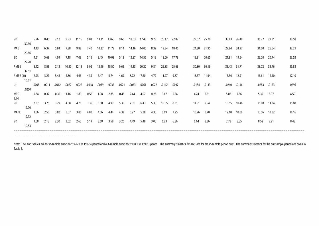
SD 5.76 8.45 7.12 9.93 11.15 9.01 13.11 13.65 9.60 18.03 17.40 9.79 25.17 22.07 29.07 25.70 33.43 26.40 36.77 27.81 38.58 30.36 MAE 4.13 6.37 5.84 7.38 9.88 7.40 10.27 11.78 8.14 14.16 14.00 8.39 19.84 18.46 24.30 21.95 27.84 24.97 31.00 26.64 32.21 29.86 SD 4.51 5.69 4.09 7.18 7.08 5.15 9.45 10.08 5.13 12.87 14.56 5.13 18.06 17.78 18.91 20.65 21.91 19.54 23.20 20.74 23.52 22.70 RMSE 6.12 8.55 7.13 10.30 12.15 9.02 13.96 15.50 9.62 19.13 20.20 9.84 26.83 25.63 30.80 30.13 35.43 31.71 38.72 33.76 39.88 37.51 RMSE (%) 2.93 3.27 3.48 4.86 4.66 4.39 6.47 5.74 4.69 8.72 7.60 4.79 11.97 9.87 13.57 11.94 15.36 12.91 16.61 14.10 17.10 16.01 U2 .0008 .0011 .0012 .0022 .0022 .0018 .0039 .0036 .0021 .0073 .0061 .0022 .0142 .0097 .0184 .0133 .0240 .0146 .0283 .0163 .0296 .0200 MPE 0.84 0.37 -0.32 1.16 1.83 -0.56 1.98 2.85 -0.48 2.44 4.07 -0.28 3.67 5.34 4.24 6.61 5.02 7.56 5.39 8.37 4.50 9.74 SD 2.37 3.25 3.79 4.38 4.28 3.36 5.60 4.99 5.35 7.31 6.43 5.30 10.05 8.31 11.91 9.94 13.55 10.46 15.08 11.34 15.88 12.70 MAPE 1.86 2.50 3.02 3.37 3.86 4.00 4.66 4.44 4.32 6.27 5.38 4.30 8.69 7.25 10.76 8.70 12.18 10.00 13.56 10.82 14.16 12.32 SD 1.68 2.13 2.30 3.02 2.65 5.19 3.68 3.58 3.20 4.49 5.48 3.00 6.23 6.86 6.64 8.36 7.78 8.35 8.52 9.21 8.48 10.53 ------------------------------------------------------------------------------------------------------------------------------------------------------------------------------------------- Note: The A&S values are for in-sample errors for 1976:3 to 1987:4 period and out-sample errors for 1988:1 to 1990:3 period. The summary statistics for A&S are for the in-sample period only. The summary statistics for the out-sample period are given in Table 3.

Table 3: Comparative analysis of forecasting accuracy of the A&S Model forecast, BCIS forecast and DL&E estimated point forecast (1988:1 - 1990:4) ------------------------------------------------------------------------------------------------------------------------------------------------------------------------------------------- Forecast horizon 0 1 2 3 4 5 6 7 8 DL&E BCIS A&S DL&E BCIS A&S DL&E BCIS A&S DL&E BCIS A&S DL&E BCIS A&S DL&E BCIS A&S DL&E BCIS A&S DL&E BCIS A&S DL&E BCIS A&S ---------------------------------------------------------------------------------------------------------------------------------------------------------------------------------- ME 5.57 7.18 -0.54 7.25 12.00 -2.10 13.17 15.27 -3.83 17.33 18.09 -6.48 21.67 19.27 18.50 18.27 16.92 13.55 10.58 8.73 4.25 5.45 SD 8.57 7.57 8.72 14.30 11.49 0.43 18.76 18.21 2.11 28.44 25.48 4.21 42.67 32.75 48.51 37.13 56.96 37.81 60.93 36.18 63.16 36.40 MAE 7.33 5.55 8.30 13.08 14.73 10.44 18.83 20.36 12.63 27.50 25.91 15.89 39.33 30.36 44.67 32.09 50.42 32.82 53.42 30.00 54.58 28.55 SD 7.19 7.20 2.73 9.27 7.69 9.65 13.06 12.25 11.79 18.79 17.47 14.56 27.25 22.84 26.47 26.13 31.45 23.16 31.16 22.03 32.05 25.23 RMSE 10.27 10.43 8.74 16.03 16.61 11.26 22.92 23.76 13.46 33.31 31.25 17.60 47.85 38.00 51.92 41.38 59.42 40.17 61.84 37.22 63.30 36.80 RMSE (%) 3.21 3.32 2.78 5.01 5.29 3.56 7.16 7.57 4.28 10.41 9.96 5.59 14.95 12.11 16.23 13.18 18.57 12.80 19.33 11.86 19.78 11.72 U2 .0010 .0011 .0008 .0025 .0028 .0013 .0051 .0066 .0018 .0108 .0099 .0031 .0223 .0146 .0262 .0173 .0343 .0016 .0372 .0140 .0390 .0137 MPE 1.77 2.27 -0.18 2.27 3.75 -0.69 4.04 4.77 -1.27 5.36 5.68 -2.13 6.83 6.13 5.90 5.88 5.59 4.39 3.65 2.87 1.81 1.86 SD 2.69 2.40 2.80 4.49 3.74 3.56 5.97 5.83 4.15 9.13 8.22 5.28 13.90 10.62 15.75 12.04 18.52 12.24 19.78 11.72 20.56 11.86 MAPE 2.29 2.38 2.65 4.10 4.67 3.33 5.93 6.46 4.04 8.73 8.24 5.09 12.60 9.70 14.28 10.26 16.11 10.50 17.08 9.63 17.45 9.21 SD 2.26 2.29 0.91 2.92 2.50 1.43 4.10 3.88 1.59 5.99 5.65 2.54 9.01 7.50 8.88 8.61 10.71 7.67 10.63 7.26 11.01 7.70 -------------------------------------------------------------------------------------------------------------------------------------------------------------------------------------------