epidemiology: study design and data analysis - spa · epidemiology: study design and data analysis...

Vetter: Epidemiology and Clinical Research 1

Thomas R. Vetter, M.D., M.P.H.

Maurice S. Albin Professor of Anesthesiology

Vice Chair and Director, Division of Pain Medicine

Department of Anesthesiology

University of Alabama School of Medicine

Birmingham, Alabama

© 2012 Thomas R. Vetter

Epidemiology: Study Design and Data Analysis

Two Introductory Observations

“A little knowledge is a dangerous thing, but a little want of knowledge is also a dangerous thing.”

Samuel Butler (1835-1902)

“For some, epidemiology is too simple to

warrant serious consideration, and for others it is too convoluted to understand. I hope to demonstrate to the reader that neither view is correct.”

Kenneth J. Rothman Epidemiology: An Introduction, 2002


My Presentation Objectives

Practical basics of biostatistics, including sample size, power analysis, and confidence intervals

Practical basics of clinical epidemiology

Sources of bias in study design

Concept of confounding in study design

Methods to identify and to control for bias and confounding, including regression modeling and propensity scores

Readily available, user-friendly biostatistics and epidemiology software options for the clinical researcher

Excellent Introductory Resources Primer of Biostatistics 7th Edition, 2011 Glantz

Medical Statistics 4

th Edition, 2007

Campbell, Machin & Walters

Epidemiology and Biostatistics 1st Edition, 2009 Kestenbaum


More Excellent Introductory Resources

Epidemiology: An Introduction 1st Edition, 2002 Rothman

Epidemiology Kept Simple 2

nd Edition, 2003

Gerstman

Designing Clinical Research 3rd Edition, 2006 Hulley, Cummings, Browner, Grady & Newman

U Penn Center for Clinical Epidemiology and Biostatistics (CCEB): Volume 1

www.cceb.upenn.edu/pages/localio/EPI521

Excellent Intermediate Resources

Modern Epidemiology 3rd Edition, 2008 Rothman, Greenland, & Lash

Practical Statistics for Medical Research 1991, Altman

Epidemiology: Study Design and Data Analysis 2nd Edition, 2004 Woodward

U Penn Center for Clinical Epidemiology and Biostatistics (CCEB): Volume 2

www.cceb.upenn.edu/pages/localio/EPI521


StatSoft: www.statsoft.com/textbook

“StatSoft has freely provided the Electronic Statistics Textbook

as a public service for more than 12 years now.”

StatPages: http://statpages.org/

“The web pages listed below comprise a powerful, conveniently-accessible, multi-platform statistical

software package. There are also links to online statistics books, tutorials, downloadable software, and

related resources. All of these resources are freely accessible, once you can get onto the Internet.”


GraphPad: http://graphpad.com

Great set of pretty easy to use calculators – not SA, Stata, SPSS, or Minitab – but it’s free!

OpenEpi 2.3.1: www.openepi.com

“A Collaborative, Open-Source Project in Epidemiologic Computing”

http://www.openepi.com/


Fundamentals of Inferential Statistics

Central Limit Theorem The distribution of means (averages) of many trials is always

normal, even if the distribution of each trial is not normal.

Law of Large Numbers Provided the sample size is large enough, the sample mean

(𝑋) will be "close" to the population mean (μ) with a specified level of probability.

The larger the sample size, the closer the sample will represent the entire population.

In practical terms, the sample N must be > about 30.

Allow us to make an inference – based upon the sample variable – about the population parameter

Types of Data

Various measurement scales

Nominal or categorical e.g., gender, race, blood type

Dichotomous or binary (+/- or yes/no) e.g., death, pregnancy, postoperative MI, PONV

Continuous or interval e.g., mean BP, serum glucose, 100 mm VAS pain score

Ordinal or rank-ordered e.g., 5 point sedation score, 11 point NRS pain score

We often collapse continuous data into dichotomous data using a “cut-point value” (< x and > x).


Measures of Central Tendency and Normal Distribution

• Mean, median, and mode are measures of central tendency.

• Mean is most sensitive to outliers.

• Examine the histograms to assess the data distribution for normality: Diastolic blood pressure are normally distributed whereas triglycerides are skewed (to the left)

• Parametric data are normally distributed versus non-parametric data are not.

• Ordinal data are always non-parametric and should be described with a median (IQR).

McCrum-Gardner, E. Which is the correct statistical test to use? Br J Oral Maxillofac Surg, 2008;46(1), 38-41.

What Test Statistic to Used?

Data Unpaired Paired > 2 Measurements per study subject

Unpaired

Continuous (interval)

Independent t-test

Paired t-test

ANOVA with repeated measures

ANOVA

Ordinal or non-normally distributed continuous

Mann-Whitney U-test

Wilcoxon signed rank test

Friedman’s test Kruskal-Wallis test

Nominal or categorical

Chi-squared (χ2) test with 2 X 2 contingency table (Fisher’s exact if any cell size is < 5)

McNemar’s test

Cochran’s Q test Chi-squared (χ2) test with 2 X N contingency table (Fisher’s exact if any cell size is < 5)

Two Groups Three or

More Groups Two Groups Two Groups

Glantz SA: Primer of Biostatistics, 7th Edition, 2011.


Hypothesis Testing I H0: the null hypothesis: 1 = 2

Ha: the alternative hypothesis: 1 ≠ 2

is population mean but could be ρ (proportion)

Is the difference observed between study sample 1 and study sample 2 significant enough to reject the H0 and accept the Ha?

“We hypothesized that _____ was more effective than _____ in treating ______ in _____.”

“This study was undertaken to assess the efficacy of ____ in reducing the incidence of _______ in _____.”

Both statements are the alternative hypothesis.

Hypothesis Testing II Type I error

Rejecting H0 when it is in fact true False positive study

Probability of Type I error = , usually set at 0.05 Increased risk with repeated measurements

Type II error Accepting Ha when it is in fact false False negative study Probability of Type II error = β, usually set at 0.20

P-value = chance of a committing a Type I error or that the observed sample difference is due simply to chance and not the intervention/factor being studied

Really no such thing as “very significant” (p < 0.01) or “highly significant” (p < 0.001): instead it’s all-or-none


So You Reject the Null Hypothesis But is the observed difference clinically significant?

Effect size for continuous data: Cohen's d = [mean group 1] – [mean group 2]

Pooled standard deviation

0 to 0.3 "small" effect

0.3 to 0.6 "medium" effect

> 0.6 to theoretically ∞ "large" effect

Number needed to treat (NNT) for dichotomous data: NNT = 100 ÷ ARR (absolute risk reduction)

Many online calculators for both Cohen’s d and NNT http://www.uccs.edu/~faculty/lbecker/

http://graphpad.com/quickcalcs/NNT1.cfm

http://www.uccs.edu/~faculty/lbecker/

Simple interface to determine effect size (Cohen’s d)









Simple interface to determine number needed to treat (NNT)

Sample Size and Power Analysis I

As N ∞, any ∆ becomes “statistically significant” Ethically must expose the least number of patients to

the risks of the study or not being optimally treated Power analysis done to determine sample size (N)

Power = 1 – β: e.g., 1 – 0.20 = 0.8 or 80% Need two things to determine needed sample size:

Minimal clinically significant difference in most important (primary) clinical outcome variable

Expected sample variance (standard deviation) – can be derived from previous studies – but is often unknown

Also need to know what test statistic is indicated! Student’s t-test, Chi-square, etc.


Sample Size and Power Analysis II Slew of online options, including:

http://www.epibiostat.ucsf.edu/biostat/sampsize.html#proportions http://hedwig.mgh.harvard.edu/sample_size/size.html http://biostat.mc.vanderbilt.edu/wiki/Main/PowerSampleSize http://statpages.org/#Power http://www.stat.ubc.ca/~rollin/stats/ssize/ http://department.obg.cuhk.edu.hk/researchsupport/statstesthome.asp

“An a priori sample size determination indicated that ______ patients per group would be needed to have 90% power of detecting a pain score difference of 20 ± 20 (SD) at rest at 24 hours postoperatively with an α = 0.05.”

𝑋1 = 60 on 100 mm VAS and 𝑋2 = 80 on 100 mm VAS The standard deviation (SD) for both groups = 20

Sample Size and Power Analysis III PS 3.0 (Vanderbilt software) University of Hong Kong

But despite power analysis of N = 22, remember Law of Large Numbers (N > 30).

Nice feature of this software

http://www.epibiostat.ucsf.edu/biostat/sampsize.html

http://www.epibiostat.ucsf.edu/biostat/sampsize.html

http://hedwig.mgh.harvard.edu/sample_size/size.html

http://hedwig.mgh.harvard.edu/sample_size/size.html

http://biostat.mc.vanderbilt.edu/wiki/Main/PowerSampleSize

http://biostat.mc.vanderbilt.edu/wiki/Main/PowerSampleSize

http://statpages.org/

http://statpages.org/

http://www.stat.ubc.ca/~rollin/stats/ssize/

http://www.stat.ubc.ca/~rollin/stats/ssize/

http://department.obg.cuhk.edu.hk/researchsupport/statstesthome.asp

http://department.obg.cuhk.edu.hk/researchsupport/statstesthome.asp


Sample Size and Power Analysis IV PS 3.0 (Vanderbilt software) University of Hong Kong

But with a Chi-square with expected 60% versus 40% incidence: N must be 130 (!)

Confidence Intervals

Sample value is only a single, variable estimate of the true value or parameter in the population.

Confidence interval is the range of values within which we can be ___% confident that this true value lies.

Can be determined for a mean, proportion, or risk ratio

95% CI = 𝑋 ± 1.96*SD/√n+: where 𝑋 is the mean and n is the sample size, 1.96 is 95% z-score

90% z-score = 1.65 and 99% z-score = 2.58 so the 90% CI is narrower and the 99% CI is wider than the 95% CI for the same random sample

Larger the sample N narrower the CI


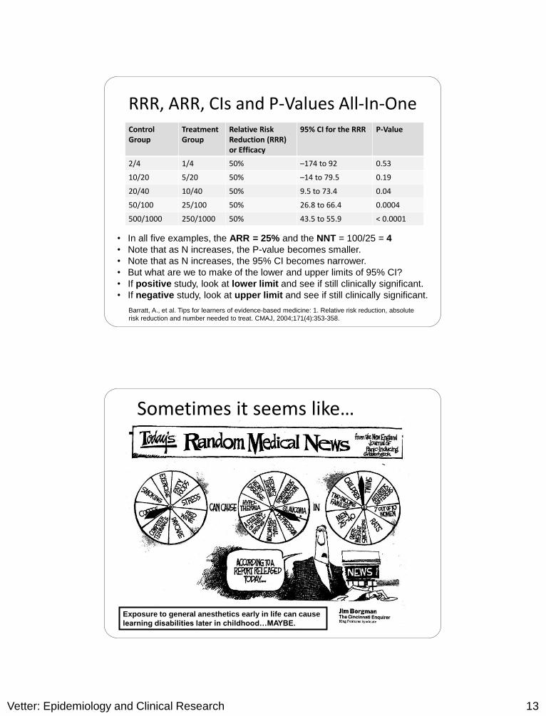
RRR, ARR, CIs and P-Values All-In-One Control Group

Treatment Group

Relative Risk Reduction (RRR) or Efficacy

95% CI for the RRR P-Value

2/4 1/4 50% –174 to 92 0.53

10/20 5/20 50% –14 to 79.5 0.19

20/40 10/40 50% 9.5 to 73.4 0.04

50/100 25/100 50% 26.8 to 66.4 0.0004

500/1000 250/1000 50% 43.5 to 55.9 < 0.0001

• In all five examples, the ARR = 25% and the NNT = 100/25 = 4

• Note that as N increases, the P-value becomes smaller.

• Note that as N increases, the 95% CI becomes narrower.

• But what are we to make of the lower and upper limits of 95% CI?

• If positive study, look at lower limit and see if still clinically significant.

• If negative study, look at upper limit and see if still clinically significant.

Barratt, A., et al. Tips for learners of evidence-based medicine: 1. Relative risk reduction, absolute

risk reduction and number needed to treat. CMAJ, 2004;171(4):353-358.

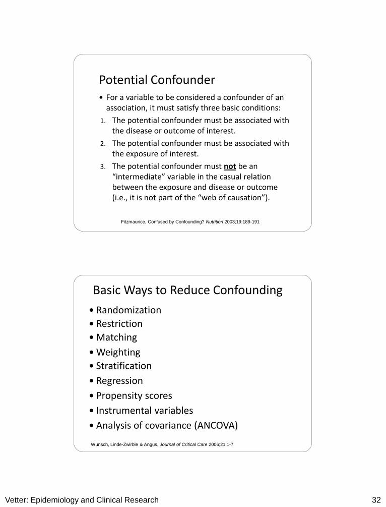
Sometimes it seems like…

Exposure to general anesthetics early in life can cause

learning disabilities later in childhood…MAYBE.


Lena S. Sun, M.D., Guohua Li, M.D., Dr.P.H., Charles DiMaggio, Ph.D., M.P.H., Mary Byrne, Ph.D., M.P.H.,

Virginia Rauh, Sc.D.,M.S.W., Jeanne Brooks-Gunn, Ph.D., Ed.M.,Athina Kakavouli, M.D., Alastair Wood, M.D.,

Coinvestigators of the Pediatric Anesthesia Neurodevelopment Assessment (PANDA) Research Network

Andrew J. Davidson, M.B., B.S., M.D., Mary Ellen McCann, M.D., M.P.H., Neil S. Morton, M.B., Ch.B., Paul S. Myles, M.D., M.P.H.

Thoughts on Clinical Trials to Address the Effects of Anesthesia on the Developing Brain

Tom G. Hansen, M.D., Ph.D., for the Danish Registry Study Group, Randall Flick, M.D., M.P.H.

Three Current Clinical Trials to Address the Effect of Anesthesia on the Developing Brain

Retrospective cohort study of children who had anesthetic exposure before age 3 yrs, the period of synaptogenesis in humans, with prospective follow-up and direct assessment Sun LS, Li G, DiMaggio C, Byrne M, Rauh V, Brooks-Gun J, Kakavouli A, Wood A, Coinvestigators of the

Pediatric Anesthesia Neurodevelopment Assessment (PANDA) Research Network: Anesthesia and neurodevelopment in children: Time for an answer. Anesthesiology 2008; 109:757–61

Prospective randomized controlled trial of healthy infants undergoing inguinal herniorraphy receiving either spinal or general anesthesia, with an N of 598 and IQ at age 5 yrs Davidson AJ, McCann ME, Morton NS, Myles PS: Anesthesia and outcome after neonatal surgery:

The role for randomized trials. Anesthesiology 2008; 109:941–4

Case-control study using very large Denmark national and Rochester (Olmstead County), MN population databases, with identification and control for a number of confounders Hansen TG, for the Danish Registry Study Group, Flick R: Anesthetic effects on the developing brain:

Insights from epidemiology. Anesthesiology 2009; 110:1–3


Public Health Epidemiology The study of the distribution of diseases in populations

and the factors that influence the occurrence of disease

Epidemiology attempts to determine who is most prone to a particular disease or outcome; where the risk of the disease or outcome is highest; when the disease or outcome is most likely to occur; how much the risk is increased through exposure; and how many cases of the disease could be avoided by eliminating the exposure

Target Population Study Population Study Sample

A “web of causation” is almost always present.

BMJ: “Epidemiology for the Uninitiated”

http://www.bmj.com/epidem/epid.html

Bradford Hill’s Attributes of Causation

Strength: stronger the association, less likely due to bias

Consistency: persons, places, circumstances and times

Specificity: one disease and one exposure relationship

Temporality: which is the cart and which is the horse?

Biological gradient: presence of a dose-response curve

Biological plausibility: makes sense given what we know

Coherence: congruent with the natural history of disease

Experimentation: evidence derived from clinical trials

Analogy: similar relationships shown with other E D

A.B. Hill, “The Environment and Disease: Association or Causation?”

Proceedings of the Royal Society of Medicine, 58 (1965), 295-300.


Clinical Epidemiology

Application of epidemiological principles and methods to questions regarding diagnosis, prognosis, and therapy

Randomized clinical trial is the prime example

Pharmacoepidemiology

Drug benefits versus adverse effects innately very applicable to anesthesiology & pain medicine

Often conducted after the drug has been marketed

Clinical Outcomes and Comparative Effectiveness Research

Epidemiologic methods plus clinical decision analysis and an economic evaluation to determine optimal treatment

Patient-reported outcome of health-related quality of life

Phase 2 Translational or Implementation Research (NIH/AHRQ)

Efficacy, Effectiveness versus Efficiency The evaluation of a new or existing healthcare intervention

or treatment involves one or more of three steps:

Efficacy Achieving its stated clinical goal

Demonstrated under optimal circumstances in a prospective randomized controlled trial (RCT) – but the results are limited to the study subjects

Effectiveness Producing greater benefit than harm

Assessed under ordinary circumstances in the more general population often by way of an observational yet analytic longitudinal cohort study

Efficiency Health status improvement for a given amount of resources ($) expended

Determined via a cost-effectiveness analysis or cost-utility analysis

Robinson & Vetter (2009): Healthcare Economic Evaluation of Chronic Pain


Prevalence versus Incidence Incidence = # of new outcomes or cases of the disease

Prevalence = # of existing outcomes or cases of the disease

Proportion – ranges from 0% to 100%

Point prevalence – at a specific point in time

Period prevalence – over a more sustained time period

The longer the duration of a condition or disease, intuitively, the greater the prevalence of the disease

Prevalence Incidence X Average Duration of Disease

Common cold has a high incidence but a short duration low point prevalence

Type II DM has a lower incidence but a long duration higher point prevalence

Cumulative Incidence Cumulative incidence is the most common way to

estimate risk in the source population of interest

Cumulative incidence (CI) = quotient of

# of new cases observed during the follow-up period

# of disease-free subjects at start of follow-up period

A few examples:

Postoperative emergence delirium with sevoflurane

Persistent incisional pain 3 months after thoracotomy

3-year IQ deficit after receiving a neonatal anesthestic

5-year mortality after aprotinin versus tranexamic acid use

10-year myocardial infarction with HDL < 40 mg/dL


Basic Study Design Schematic

Comparative Studies

Observational

Cross-sectional studies

Cohort studies

Case-control studies

Experimental Clinical Trials

Individually randomized

controlled trials

Cluster randomized

controlled trials

www.gfmer.ch/PGC_RH_2005/pdf/Cluster_Randomized_Trials.pdf

Hierarchy of Risk Estimation Studies

Modified from Kraemer, Lowe & Kupfer, To Your Health:

How to Understand What Research Tells Us About Risk (2005), pg. 107

RCT is considered the gold standard and proverbial holy grail in clinical research.


What’s Wrong with an RCT?

Highly restricted study subject eligibility based upon well-defined inclusion and exclusion criteria – can make study enrollment protracted

Ethical and logistical constraints preclude using an RCT design to answer certain questions – often more complex, “real-world” challenges.

Minorities and both age extremes – pediatric and geriatric patients – are conventionally excluded despite equal or greater clinical need.

The results of an RCT often lack external validity and cannot be generalized to the more diverse population – with co-existing diseases.

Simple randomization may not sufficiently control for confounding variables.

Rochon et al., BMJ 2005;330:895-897

1. Cross-Sectional Study

Examines the relationship between potential risk factors

and outcomes during a short period of time (“snapshot”)

Potential risk factors or outcomes are not likely to change

during the duration or time frame of the study.

Cross-sectional study estimates the point prevalence.

Valuable as pilot study to establish tentative association

Generate hypotheses for more rigorous studies

Examples: Co-existing depression among patients

presenting to a chronic pain medicine clinic; positive

pregnancy test among pediatric surgical outpatients


2. Cohort Study Longitudinal study of E D risk relationship (forward)

Single exposure with multiple subsequent outcomes

At the outset of study all participants are outcome-free

Natural or self-selection into risk categories

During follow-up period participants are reassessed as to

whether the outcome has occurred.

Time-consuming and costly to perform if prospective

Loss to follow-up and differential attrition can lead to bias

(systematic error) and thus validity issues.

An RCT represents an experimental form of cohort study.

What is Risk? Risk: The probability of an outcome within a population

Likelihood a person in a population will have the outcome

Risk is a number between 0% and 100% or 0 and 1.0

The specified health outcome is binary (+/− or yes/no).

The study population must be clearly defined.

While well-defined, this population cannot be known:

thus a representative study sample is selected and an

estimated risk in this study sample is determined.

Risk estimate is for a specific and logical risk time period,

e.g., 24 hours postoperatively, 5 year follow-up.

Efficacy = (riskcontrol − riskintervention)/(riskcontrol) = RRR


What is a Risk Ratio?

A ratio is the quotient of two numbers

Risk ratio = Risk in group A ÷ Risk in Group B

Risk ratio ranges from 0 to infinity (∞) with 1 = null value

In most epidemiological studies Group A and Group B

differ by way of a self-selected or natural series of events

Whereas in a randomized controlled trial (RCT) Group A

and Group B differ in a randomized yet very controlled

manner with each group receiving a specific treatment

Risk ratio allows for a comparison of the risk of the

disease or outcome in Group A versus Group B.

More appropriate for high incidence conditions

2 X 2 Table

Drug X Drug Y Total

Outcome (+) A B A+B

Outcome (−) C D C+D

Total A + C B + D A + B + C+ D

Frequency or Proportion for Drug X = A/(A+C) and

Frequency or Proportion for Drug Y = B/(B+D)

Risk for Drug X = A/(A+C) and Risk for Drug Y = B/(B+D)

Risk Ratio = [A/(A+C)] ÷ [B/(B+D)]


OpenEpi 2.3.1: www.openepi.com

Menu Counts Folder Two by Two Table: 2X2 Contingency Table

Nurse-Controlled Analgesia

Neonate Older

1 Month Total

Serious Adverse

Event (+) 13 26 39

Serious Adverse

Event (−) 497 9543 10049

Total 510 9569 10079

Risk for Neonate = 13/510 = 0.025 or 2.5%

Risk for Older 1 Month = 26/9569 = 0.0027 or 0.27%

Risk Ratio or Relative Risk = 0.025/0.0027 = 9.4 (4.8,18.2)

Howard et al., Nurse-Controlled Analgesia (NCA) Following Major Surgery in 10000 Patients

in a Children’s Hospital, Pediatric Anesthesia 2010;20:126-134

http://www.openepi.com/


Risk and Risk Reduction: Definitions Event rate

Number of people experiencing an event as a proportion of the number of people in the sample or population

Relative risk reduction

Difference in event rates between 2 groups, expressed as a proportion of the event rate in the untreated group; usually constant across populations with different risks

Absolute risk reduction

Arithmetic difference between 2 event rates; varies with the underlying risk of an event in the individual patient

Barratt, A., et al. Tips for learners of evidence-based medicine: 1. Relative risk reduction, absolute risk

reduction and number needed to treat. CMAJ, 2004;171(4):353-358

Risk Difference and the Number Needed to Treat

Risk Difference or Cumulative Incidence Difference (CID) =

CI1 − CI0 with 1 = those exposed and 0 = unexposed

Absolute Risk Reduction (ARR) in clinical epidemiology

Number Needed to Treat (NNT) = 1/(CI1 − CI0) = 1/ARR

Number Needed to Harm (NNH) in the case of an

untoward event (stroke, MI, death) or an adverse side

effect (respiratory depression, persistent paresthesia)

Far more germane than a simple p-value


Basic Example of RRR, ARR, NNT

0%

5%

10%

15%

20%

25%

30%

35%

40%

45%

Trial 1:High Risk

Group

Trial 2:Low Risk

Group

Control

Treated

High risk group

RRR = [40% – 30%] /40% = 25%

ARR = 40% – 30% = 10%

NNT = 100/10 = 10

Low risk group

RRR = [10% – 7.5%] /10% = 25%

ARR = 10% – 7.5% = 2.5%

NNT = 100/2.5 = 40

Lower the event rate control group, larger the difference between RRR and ARR

RRR efficacy Barratt, A., et al. Tips for learners of evidence-

based medicine: 1. Relative risk reduction, absolute

risk reduction and number needed to treat. CMAJ,

2004;171(4):353-358.

Hypothesis Testing

In an RCT versus in a prospective cohort study

RCT Ho: P1 − P0 = 0 or P1 = P0 and Ha: P1 − P0 ≠ 0 or P1 ≠ P0

P = proportion of the study group with the outcome

Cohort Study Ho: RR = CI1/CI0 = 1 and Ha: RR = CI1/CI0 ≠ 1

RR = risk ratio

CI = cumulative incidence of the disease or outcome in cohort

A cohort study and an RCT are essentially asking the same

questions: what is the effect of the exposure (treatment)

on the disease (outcome) and is it significant?


Postoperative Nausea & Vomiting

Clonidine Caudal

(2 mcg/kg)

Hydromorphone Caudal

(10 mcg/kg)

(+) PONV 10 (50% incidence) 18 (90% incidence)

(−) PONV 10 2

Total 20 20

PONV Risk 10 ÷ 20 = 0.5 18 ÷ 20 = 0.9

Fisher’s exact test P = 0.014 (because a cell size < 5)

Risk ratio (RR) = 0.9 ÷ 0.5 = 1.8 PONV 1.8 times as likely

Absolute risk reduction (ARR) = 0.9 − 0.5 = 0.4 or 40%

Number needed to treat (NNT) = 1 ÷ 0.4 = 2.5 patients

Ketamine and Hallucinations

Incidence and risk of hallucinations in awake or sedated

patients not receiving a benzodiazepine was high:

Risk of 10.43% versus risk of 5.70% 4.73% risk difference

Risk ratio of 2.32 (95% CI, 1.09 – 4.92)

Number needed to harm = 1 ÷ (0.1043 − 0.057) = 21

In anesthetized patients the incidence of hallucinations was

low and independent of benzodiazepine administration:

Risk of 0.76% versus risk of 0.41% 0.35% risk difference

Risk ratio of 1.49 but not significant (95% CI, 0.18 – 12.6)

Number needed to harm = 1 ÷ (0.0035) = 286

Elia & Tramer, Pain 2005;113:61-70


3. Case-Control Study

Is the observed outcome related to the exposure?

Outcome or disease is observed first: E D (backward)

Single outcome with multiple previous exposures

Cases are subjects with the outcome of interest

Controls are subjects without the outcome of interest

Controls sampled from the same source population but must be sampled independently of their exposure status

Less costly and less time-consuming than cohort study

Efficient for rare outcomes

Cannot generate an overall risk or rate estimate but instead an odds ratio is determined and not a risk ratio

Probability versus Odds Probability (P)

Number of times an outcome occurs out of the total # of attempts

Ranges from 0 to 1

“Epi Beauty” won 30 of 50 races P of winning is 30/50 = 0.60

Odds P ÷ (1 − P) = probability of winning ÷ probability of losing Ranges from 0 to infinity (∞) Horse race: Odds of winning = 0.6/(1 − 0.6) = 0.6/0.4 = 1.5 to 1

Odds Ratio Ratio of the odds of the disease or clinical outcome with

the exposure versus without the exposure


2 X 2 Table Revisited

Outcome (+)

Cases with Disease

Outcome (−)

Controls

w/o Disease

Exposure (+) A B

Exposure (−) C D

• A and C are selected based on disease (outcome) status

• We cannot calculate the rate or risk of getting the disease (outcome)

because we do not know the denominator (size of study population)

• Odds = number of cases with disease ÷ number of non-cases of disease

• Odds with exposure = (A/B) and odds without exposure = (C/D)

• Odds ratio with versus without exposure = (A/B) ÷ (C/D) = AD/BC

Perioperative Questions That Could Be Addressed by a Case-Control Study

Rare outcomes with several possible exposure risk factors

What are the risk factors for malignant hyperthermia?

Is epidural catheter placement under general anesthesia a risk factor for postoperative paraplegia?

Does pulse oximetry and/or end-tidal capnography decrease the risk of perioperative brain anoxia?

Does neonatal anesthesia cause later cognitive deficits?

Is nurse or parent proxy-patient controlled analgesia (PCA) a risk factor for respiratory depression or arrest?

Examples of fertile ground for case-control studies: ASA Closed Claims Project Pediatric Perioperative Cardiac Arrest (POCA) Registry Multicenter Perioperative Outcomes Group (MPOG)


Patient-Controlled Analgesia by Proxy

Threshold Event (TE) = ↓O2 saturation, bradypnea, & oversedation

Rescue Event (RE) = naloxone, airway intervention, & escalation of care (to ICU)

TE (+) TE (−) Total

PCA-Proxy 21 124 145

PCA w/o Proxy 37 120 157

RE (+) RE (−) Total

PCA-Proxy 11 134 145

PCA w/o Proxy 1 156 157

Exposure odds ratio =

(21 X 120) ÷ (124 X 37) =

0.54 (0.30 − 0.99)

Χ2 test P < 0.015 versus

Χ2 test P = 0.045 actual

Exposure odds ratio =

(11 X 156) ÷ (134 X 1) =

12.8 (1.6 − 100.0)

Χ2 test P < 0.015

Χ2 test P = 0.005 actual

Voepel-Lewis et al., The Prevalence of Risk Factors for Adverse Events in Children Receiving

Patient-Controlled Analgesia by Proxy or Patient-Controlled Analgesia after Surgery

Anesthesia & Analgesia 2008;107:7-75

Two Other Types of Study Design

Nested case-control study

A case-control study that is set or nested within an existing cohort study or even an intervention study like an RCT

Greatest advantage of nested study is that cases and controls come from the same population, which avoids selection bias.

Cluster randomized trial

Study subjects in an intervention study naturally occur in separate groups or clusters (e.g., geographic location)

Rather than randomize individuals to treatment, randomize based upon the clusters (e.g., hospital, surgical service)

Often applied for convenience or out of necessity

Deceptively simple to construct and data analysis is complex


Sources of Error in Study Design

Random Error: simple variability in the sample data

Systematic Error or Bias: 3 basic types

Selection Bias Individuals have different probabilities of being in the study

sample based upon relevant characteristics (E and D) Differential loss to follow-up – including in an RCT

Information Bias Misclassification of exposure and/or disease (outcome) status,

validity of diagnosis as measured by sensitivity and specificity Observer bias is mitigated via blinding (masking) in an RCT

Confounding Effect of the exposure of interest is mixed together with and

confused by the effect of one or more other variables

Random Error versus Systematic Error

Rothman, Epidemiology: An Introduction (2002), pg. 95

As N increases, the SEM decreases and thus 95% CI becomes narrower

Estimate (variable) = parameter + random error + systematic error


Example of Confounding

1000 subjects, age 50-55 years, followed for 15 years:

Risk with vitamin E supplement use = 50/550 = 0.09 (9%)

Risk w/o vitamin E supplement use = 66/450 = 0.15 (15%)

Risk ratio = 0.09/0.15 = 0.62; P = 0.008

Risk odds ratio (crude) = (50 X 384) ÷ (500 X 66) = 0.58

Vitamin E appears cardio-protective…but is it really?

CAD Present CAD Absent

Vitamin E Supplement (+)

50 500

Vitamin E Supplement (−)

66 384

Fitzmaurice, Confused by Confounding? Nutrition 2003; 19:189-191

Example of Confounding (Cont’d)

Smokers

Non-Smokers



10 40


50 200



40 460


16 184

Stratum risk odds ratio =

(10 X 200) ÷ (40 X 50) = 1.0

P = 0.85

Stratum risk odds ratio =

(40 X 184) ÷ (460 X 16) = 1.0

P = 0.88

Fitzmaurice, Confused by Confounding? Nutrition 2003;19:189-191

There is no association

between vitamin E supplement

and CAD after controlling for

the effects of smoking.

Stratum-specific odds ratios

are similar in magnitude


Interaction versus Confounding Confounding (from the Latin confundere meaning “to mix

together”): an undesirable distortion of the association between an exposure (E) and disease (D) brought about by extraneous factors (C1, C2, etc).

Interaction: “effect modification” whereby the effect on the response (y) of one explanatory variable (x) depends on the level of one or more other explanatory variables

Two-way or two factor model: y = b0 + b1x1 + b2x2 + b3x1x2

The joint effect of two or more explanatory variables is larger or smaller than the sum of the parts.

b3x1x2 = interaction term tested with H0: b3 = 0

Synergism (from the Greek sunergos meaning “working together”) is a type of biological interaction.

Interaction versus Confounding

Interaction Confounding

Smoking (C) amplifies the risk of thromboembolic disease (D) with oral contraceptive use (E).

Interaction exists between the interdependent risk factors of smoking (C) and oral contraceptive use (E).

This effect modification is biological synergism.

Smoking (C) confuses the relationship between alcohol consumption (E) and lung cancer (D).

Since alcohol and smoking are related, and smoking (C) is an independent risk factor for lung cancer (D).

This extraneous factor results in confounding.

Woodward, Epidemiology: Study Design and Data Analysis (2005)

Rothman, Greenland, & Lash, Modern Epidemiology (2008)


Potential Confounder For a variable to be considered a confounder of an

association, it must satisfy three basic conditions:

1. The potential confounder must be associated with the disease or outcome of interest.

2. The potential confounder must be associated with the exposure of interest.

3. The potential confounder must not be an “intermediate” variable in the casual relation between the exposure and disease or outcome (i.e., it is not part of the “web of causation”).

Fitzmaurice, Confused by Confounding? Nutrition 2003;19:189-191

Basic Ways to Reduce Confounding

Randomization

Restriction

Matching

Weighting

Stratification

Regression

Propensity scores

Instrumental variables

Analysis of covariance (ANCOVA)

Wunsch, Linde-Zwirble & Angus, Journal of Critical Care 2006;21:1-7


Techniques to Adjust for Confounding in Observational Studies

Wunsch, Linde-Zwirble & Angus, Journal of Critical Care 2006;21:1-7

Randomization Randomization is only applicable in an experimental

study in which exposure is assigned or controlled.

With a large enough sample size (N), randomization produces two or more study groups with nearly the same distribution of the study subject (patient) characteristics that are plausible confounding variables.

Randomization also reduces confounding by any other unidentified factors or variables.

But randomization is not always feasible or ethical, especially in retrospective studies or longitudinal observational studies.


Restriction Often applied in addition to randomization

Study inclusion and even more so study exclusion criteria control for the identified confounders.

Trade-off is that study findings are assuredly valid only for the restricted study population from which the study sample is drawn.

This external validity issue must be considered in generalizing findings to a more diverse population.

One of the challenges of applying evidence-based medicine in one’s daily practice: Are these study findings applicable to my given patient?

Matching Individuals from the two study groups are paired

based upon the presumed confounding variables.

Allows for even distribution of potential confounders

Most often applied in case-control studies

Age, sex, race are common matching variables.

Expensive and time consuming

Reduces the power of the study because not all study subjects can be matched

Does not assuredly control for other confounders and in fact can introduce hidden confounding

Restriction in an RCT is a “loose” form of matching.


Assessing for Confounding in RCT I In almost all clinical trials, the study groups are compared

using parametric or non-parametric statistics for any differences in baseline characteristics: Demographics

Anthropometrics

Other pertinent clinical variables

Absence of “statistically significant” difference is often taken to indicate study group comparability and a lack of confounding by these covariates.

More conservative p-value of 0.20 may be better

Residual cofounding may be present despite p > 0.05

The results of a statistical test for significant difference – “the almighty p-value” – depend on the sample size (N): As N ∞, any observed difference achieves a p < 0.05

With a larger N, there is a greater likelihood of baseline difference

Assessing for Confounding in RCT II

Ho: ρ1 = ρ2 with ρ = population proportion (parameter) or μ1 = μ2 with μ = population mean (parameter)

Ho rejected if p < 0.05 But in assessing for confounding in an RCT our required

assumption or the Ho: Any imbalance between the study groups in a baseline clinical feature or risk factor is simply due to chance and not randomization

But successful randomized allocation requires that any observed imbalance must be due to chance

The Ho thus cannot be rejected (!) even with a p < 0.05 A statistically significant imbalance in a baseline risk

factor in and of itself does not reflect the amount of confounding instead we need to determine how much of an effect does the risk factor have on the outcome?

Rothman, Epidemiology: An Introduction (2002), page 209


Stratification

One of the most effective techniques for adjusting for the effects of confounding in an analysis

Association is evaluated within distinct groups, or strata, comprised of individuals who are relatively homogenous in terms of the confounding variable.

A crude overall estimate of association is adjusted for the confounding variables.

Generated by taking a weighted average of the stratum-specific estimates of association.

Requires stratum-specific estimates of association to be uniform across the levels of the potential confounder. Otherwise stratum-specific estimates should be reported.

Assessing for Confounding in RCT III

Better approach for dichotomous (binary) outcomes:

1. Control for the confounder using conventional study design with study subject randomization and restriction

2. Determine the potentially confounded crude results

3. Stratify the results on the potential confounding variables (e.g., age and gender) and then determine pooled Mantel-Haenszel adjusted results

4. Compare the crude results with the adjusted results

5. If the two estimates are comparable conclude that confounding is not present

6. If two estimates are “meaningfully different” (> 10%) conclude that confounding is present


Cochran-Mantel-Haenszel Method

j levels of the stratification variable (e.g., two strata for male and female)

Create a series of stratum-specific 2X2 contingency tables

j total number of 2x2 contingency tables

nj = total number of observations in the jth table = (aj + bj+ cj + dj)

Disease or Outcome

(+)

Disease or Outcome

(−)

Exposure (+) aj bj

Exposure (−) cj dj

• One of the most widely used methods for combining or pooling stratum-specific estimates of association • Generates an adjusted estimate of association (odds ratio) • Can also generate an adjusted estimate of risk ratio

Example of Mantel-Haenszel Method I

Smokers

Non-Smokers

CAD (+) CAD (−)

Vitamin E Supplement (+) 11 40

Vitamin E Supplement (−) 49 200

CAD (+) CAD (−)



Crude odds ratio = 0.59

(95% CI, 0.40 − 0.87)

Stratum odds ratio = 0.97

(95% CI, 0.53 − 1.78)

Fitzmaurice, Adjusting for Confounding, Nutrition 2004; 20:594-596

CAD (+) CAD (−)



Entire Cohort


(95% CI, 0.54 − 2.34)

MH adjusted odds ratio = 1.03

(95% CI, 0.64 − 1.65)

INTERACTION is not present

between vitamin E supplement

and smoking because the

stratum-specific odds ratios

are not significantly different.

CONFOUNDING


Example of Mantel-Haenszel Method II

African-Americans

Whites

SGA (+) SGA (−)

Smoked during pregnancy (+) 21 180

Smoked during pregnancy (−) 64 702

SGA (+) SGA (−)



Crude odds ratio = 2.55

(95% CI, 1.91 − 3.40)


(95% CI, 2.52 − 5.56) Modified from Savitz et al., Epidemiology 2001;12:636-642

SGA (+) SGA (−)



Smoking and Pregnancy Outcome among African-American and

White Women: The Risk for a Small for Gestational Age (SGA) Newborn

Entire Cohort


(95% CI, 0.76 − 2.15)

MH adjusted odds ratio = 2.56

(95% CI, 1.89 − 3.45)

INTERACTION may be present

between race and smoking

b/c the stratum-specific odds

ratios are significantly different

NO CONFOUNDING

Regression When there are many potential confounding variables, (k),

the resulting strata (2k) have too few individuals to generate a precise estimate of association.

Alternatively, estimate the exposure effect of interest using a regression model for the dependence of the disease (outcome) on the primary exposure and any potential confounding variables.

Assess the effect of the use of vitamin E supplements on CAD, while controlling for or adjusting for not only smoking history but also other potential confounders (e.g., age, BMI, physical activity, LDL, HgbA1C)

Requires assumptions be met and a larger sample size and does not ensure confounder distributions are comparable

Fitzmaurice, Confounding: Regression adjustment, Nutrition 2006;22:581-583


Methods of Regression I Simple linear regression: single continuous outcome

variable (y) and a single predictor variable (x)

y = b1x1 + b0 + ε

b1 = slope and b0 = intercept and ε = error (∆y)

Multiple linear regression: single continuous outcome (y) but instead multiple predictor variables (x1, 2, 3…k)

y = b0 + b1x1 + b2x2 + b3x3 + …+ bkxk + ε

The predictor variables (x1,x2,x3 …) can be continuous (age), ordinal (ASA status), and/or dichotomous (sex) in a linear regression model.

But you need at least 10 observations (study subjects) for each x variable placed in the model plus other assumptions must be met

Three Studies Addressing the Effect of Maternal Fish Intake and Smoking on the Child Neurodevelopment

After adjusting for 28 potential confounders, maternal seafood intake during pregnancy of < 340 gm per week was associated with increased risk of their children being in the lowest quartile for verbal intelligence quotient (IQ): No seafood consumption, odds ratio [OR] 1·48, 95% CI 1·16–1·90 (N = 11,875). Hibblen JR et al: Maternal seafood consumption in pregnancy and neurodevelopmental outcomes in

childhood (ALSPAC study): An observational cohort study. Lancet 2007; 369:578-85.

Using multivariate linear regression, in 4 year old children breast-fed for < 6 months, maternal fish intakes of > 2–3 times/week were associated with significantly higher scores on several McCarthy Scales of Children’s Abilities (MSCA) subscales compared with intakes < 1 time/week (N = 392). Mendez MA et al: Maternal fish and other seafood intakes during pregnancy and child neurodevelopment

at age 4 years. Public Health Nutrition 2008; 12(10):1702-1710.

Using multivariate linear regression, maternal smoking during pregnancy (in cigs/day) was associated with a decrease in child’s MSCA global cognitive score *β = 0.60, (95% CI: 1.10; 0.09)+ in offspring at age 4 years (N = 420). Julvez Jet al: Maternal smoking habits and cognitive development of children at age 4 years in a population-

based birth cohort. International Journal of Epidemiology 2007;36(4):825-32.


Linear regression may not always work Simple and multiple linear regression is applied when

the outcome variable (y) is continuous.

But what happens if:

1. The outcome variable (y) is not linearly related to the predictor variables (x)?

2. The outcome variable (y) is risk that ranges from 0 to 1?

3. The outcome variable (y) is not continuous but instead dichotomous/binary (0 = no, 1 = yes) like risk of death?

Then you apply a logistic regression model…

Logistic Function

y = 1/*1 + exp(−b0 − b1x1)]

r = risk = 1/*1 + exp(−b0 − b1x1)]

r

x1


Methods of Regression II Simple logistic regression: single binary (1 = yes/0 = no)

outcome variable (y) and a single predictor variable (x)

p = probability of outcome of interest; odds = p ÷ (1 − p)

logit(p) = loge (odds) = loge *p/(1 − p)+ = loge (p) − loge (1 − p)

logit(p) = loge *p/(1 − p)+ = b0 + b1x1

odds ratio = loge (odds1/odds2) = loge (odds1) − loge (odds2)

odds ratio (with X1 = 1 compared to X1 = 0) = eb0 + b1x1

Multiple logistic regression: binary outcome (1 = yes/0 = no) but instead multiple predictor variables (x1, 2, 3…k)

logit(p) = loge *p/(1 − p)+ = b0 + b1x1 + b2x2 + b3x3 + …+ bkxk

odds ratio = eb0 + b1x1 + b2x2 + b3x3 + …+ bkxk

Ordinal regression: rank-ordered outcome (1, 2, 3, 4, 5)

Cox proportional hazards: time to an event of interest

Example of Regression Adjustment Maternal Diet and the Risk of Hypospadias and Cryptorchidism in the Offspring

Factor CRYPT Crude

CRYPT Adjust

HYPOSPAD Crude

HYPOSPAD Adjust

Liver & other offal (>1/week) 3.2 (0.9, 10.7) 5.2 (1.3, 14.2)

Fish (>1/week) 1.6 (0.8, 3.2) 2.3 (1.0, 5.3)

Mostly market fruit 3.5 (1.0, 11.9) 5.1 (1.3, 19.8)

Fried foods 2.0 (1.0, 3.8) 1.5 (0.7, 3.2)

Smoked foods 2.0 (1.1, 3.9) 2.5 (1.2, 5.3)

Plastic food boxes/containers 0.4 (0.2, 0.9) 0.5 (0.2, 1.2)

Mineral supplement 0.5 (0.3, 1.0) 0.5 (0.2, 1.1)

Giordano et al., Paediatric and Perinatal Epidemiology 2008;22:249-260

“This study suggests that some maternal dietary factors may play a role in the development of congenital defects of the male reproductive tract. In particular, our data indicate that further research may be warranted on the endocrine-disrupting effects resulting from the bioaccumulation of contaminants (fish, liver), pesticides (marketed fruit, wine) and/or potentially toxic food components (smoked products, wine, liver).”

Controlling for maternal age, parity, education, & GYN disease; paternal GU disease & use of pesticides


Cohort Covariate Imbalances

P P P P

P P P P P

P P P P P

P P P P

P P P

Population of patients

prescribed an NSAID

I I I I I I

I I I I I I I I I

C C C

C C

Prescribers’

decisions

• Younger • Better renal

function • Lower BP • Healthier

• Fewer drugs

• Older • Worse renal

function • Higher BP

• Sicker • More drugs

Prescribed

ibuprofen (75%)

Prescribed

celecoxib (25%)

Modified from Perkins et al., Pharmacoepidemiology and Drug Safety 2000;9:94

Cavuto, Bravi, Grassi & Apolone, Drug Development Research 2006;67:208-216

Covariate imbalances resulting from

non-randomized treatment assignment

to ibuprofen and celecoxib

Confounding by indication

Propensity Scores Propensity score = the probability (0 to 1) that a subject

would have been treated given the individual’s covariates

Intended to reduce selection bias and increase precision in non-randomized large-scale observational studies

Collapse all of the background characteristics (X1, X2, …., Xp) or confounding covariates into a single composite value

Propensity score (PS) is generated using logistic regression

PS = P(Z = 1|(X1, X2, …., Xp)} Z = 1 if exposed, Z = 0 if not exposed

PS = exp(b0 + b1x1 + b2x2 + b3x3 + …+ bkxk)

1 + exp(b0 + b1x1 + b2x2 + b3x3 + …+ bkxk)

Predictive strength: C-statistic from ROC curve = 0.5 to 1.0

Rubin, Annals of Internal Medicine 1997;127:757-763

D’Agostino, Statistics in Medicine 1998;17:2265-2281

Fitzmaurice, Confounding: Propensity score adjustment Nutrition 2006;22:1214-1216


Propensity Scores Balancing scores (“apples to oranges” “apples to apples”)

Can only adjust for observed confounding covariates

Applicable for large-scale patient registry-based clinical cohort studies of longitudinal outcomes

Creates a “quasi-randomized study” equal propensity score equal likelihood to be treated or to be a control

Requires large sample sizes to assure balance

Requires adequate overlap of propensity distributions

Randomization tends to balance the unmeasured covariates

Propensity score modeling is thus not intended for RCTs, but propensity scores can possibly be used for ANCOVA

Blackstone, Journal of Thoracic and Cardiovascular Surgery 2002;123:8-15

Glynn, Schneeweiss & Stürmer, Basic & Clinical Pharmacology &Toxicology 2006;98(3):253-259

Rubin, American Journal of Ophthalmology 2010;149(1):7-9

Non-Overlap of Propensity Scores

The non-overlap of the exposure propensity score distribution among treated and untreated study subjects makes the use of propensity scores questionable.

In this example subjects with very low propensity score are never treated while subjects with very high propensity score are all treated.

Glynn, Schneeweiss & Stürmer, Basic & Clinical Pharmacology &Toxicology 2006;98(3):253-259


Example of Use Propensity Scores

Retrospective observational case-control study undertaken to identify the independent predictors of unanticipated early postoperative respiratory failure requiring tracheal intubation after nonemergent, noncardiac surgery.

Hypothesized that unanticipated early postoperative respiratory failure is associated with a risk-adjusted increase in mortality.

Univariate crude odds ratios were all significant but confounding very likely present and interaction possibly present.

Ramachandran SK, Nafiu OO, Ghaferi A, Tremper KK, Shanks A, Kheterpal S. Independent predictors and outcomes of unanticipated early postoperative tracheal intubation after nonemergent, noncardiac surgery. Anesthesiology. 2011 Jul;115(1):44-53.

Baseline characteristics of patients with no unanticipated early postoperative intubation (No UEPI) vs. patients with unanticipated early postoperative intubation (UEPI)


Characteristics of the matched cohort (subset) of patients with No UEPI vs. patients with UEPI


Patients from the derivation cohort were risk-matched based on the propensity score of a logistic regression model. Matching was performed on a one-to-one basis for the outcome variable UEPI, and all predictor univariates were reassessed after matching to assure sufficient matching (a p > 0.05). This controlled for confounding.



After controlling for the other risk factors, based

upon the adjusted odds ratios, all of these

co-morbidities were significant risk factors for

unanticipated early postoperative intubation.


Null value of 1.0 for an ratio

Example of Use Propensity Scores Ramachandran SK, Nafiu OO, Ghaferi A, Tremper KK, Shanks A, Kheterpal S. Independent predictors and outcomes of unanticipated early postoperative tracheal intubation after nonemergent, noncardiac surgery. Anesthesiology. 2011 Jul;115(1):44-53.

Significant increases in death rate in patients with unanticipated early postoperative intubation (UEPI) across increasing risk classes.

Like the Lee Revised Cardiac Risk Index, an UEPI risk index was created.


Instrumental Variables Analysis (IVA) Covariate analysis cannot adjust for potential confounding

variables that are unknown or not easily quantifiable.

IVA exploits quasi-experimental variation in treatment assignment that is incidental to the studied health outcome.

Three assumptions for IVA:

1. The IV must predict treatment but that prediction does not have to be perfect. An IV that does a poor job of prediction is said to be weak.

2. A valid IV will not be directly related to outcome, except through the effect of the treatment.

3. A valid IV will also not be related to outcome through either measured or unmeasured paths.

Johnston, Gustafson, Levy & Grootendorst, Statistics in Medicine 2008; 27:1539–1556

Rassen et al., Journal of Clinical Epidemiology 2009;62:1226-1232

Causal Relations in IVA

General instrumental variable analysis (IVA) model

Example of IVA with physician-specific prescribing preference

Instrument Variable (Z)

Treatment (X)

Unmeasured confounders (C)

Outcome (Y)

Bennett, Methods in Neuroepidemiology 2010;35(3):237-240

Brookhart, Wang, Solomon & Scheeweiss, Epidemiology 2006;17(3):268-275


Instrumental Variables Model Two-stage least-squares regression

1. Y = α0 + α1X + ε1 } Y = outcome, X = exposure

2. X = β0 + β1Z + ε2 } X = exposure, Z = instrument variable

Substituting equation 2 into equation 1:

Y = α0 + α1 (β0 + β1Z + ε2) + ε1 Yi = γ0 + γ1Zi + εi

Estimate direct treatment effect (β1) of treatment (Ti) on outcome (Yi): β1 = γ1/α1

Examples of instrumental variables

Physician prescribing preference for NSAID

Smoking cessation program in pregnant mothers

Distance to hospital with cardiac catherization laboratory

Bennett, Methods in Neuroepidemiology 2010;35(3):237-240

Schneeweiss et al., Arthritis & Rhematism 2006;54(11):3390-3398

Brookhart, Rassen & Schneeweiss, Pharmacoepidemiology and Drug Safety 2010;19:537-554

Analysis of Covariance (ANCOVA)

Compares several means (like an ANOVA) but adjusts for the effect of one or more other variables (covariates)

These covariates can be the presumed confounders.

May use the propensity score as a single covariate (?)

Two key but often violated assumptions for an ANCOVA:

Independence of the covariate and experimental effect (x)

Homogeneity of regression slopes: the relationship between the covariate and dependent outcome (y) is true for all of the subgroups of study subjects

Use of ANCOVA is quite controversial – it is not a quick fix.

Miller & Chapman, Journal of Abnormal Psychology 2001;110:40-48

Leech, Barrett, & Morgan (2005): SPSS for Intermediate Statistics: Use and Interpretation (2nd edition)

Field (2009): Discovering Statistics Using SPSS (3rd edition)


Johns Hopkins Bloomberg School of Public Health's OPENCOURSEWARE (OCW) Project

“…provides access to content of the School's most popular courses. As challenges to the world's health escalate daily, the School feels a moral imperative to provide equal and open access to information and knowledge about the obstacles to the public's health and their potential solutions.”

Funded by the William and Flora Hewlett Foundation

Introduction to Biostatistics: http://ocw.jhsph.edu/courses/introbiostats/

Methods in Biostatistics I: http://ocw.jhsph.edu/courses/MethodsInBiostatisticsI/

Methods in Biostatistics II: http://ocw.jhsph.edu/courses/methodsinbiostatisticsii/

Fundamentals of Epidemiology I: http://ocw.jhsph.edu/courses/FundEpi/

Fundamentals of Epidemiology II: http://ocw.jhsph.edu/courses/fundepiii/

ActivEpi: www.activepi.com

“ActivEpi is a collection of innovative tools for learning epidemiology.”

Multimedia approach to learning basic and some intermediate epidemiology

Extensive series of online, downloadable PowerPoint presentations (free)

“Epi for Clinicians” section provides a population-based perspective on clinical medicine.

http://ocw.jhsph.edu/courses/introbiostats/

http://ocw.jhsph.edu/courses/MethodsInBiostatisticsI/

http://ocw.jhsph.edu/courses/methodsinbiostatisticsii/

http://ocw.jhsph.edu/courses/FundEpi/

http://ocw.jhsph.edu/courses/fundepiii/

http://www.activepi.com/


Epi Info 3.5.3: www.cdc.gov/epiinfo

“Physicians, nurses,

epidemiologists, and other

public health workers lacking

a background in information

technology often have a

need for simple tools that

allow the rapid creation of

data collection instruments

and data analysis,

visualization, and reporting

using epidemiologic

methods.

Epi Info™, a suite of

lightweight software tools,

delivers core ad-hoc

epidemiologic functionality

without the complexity or

expense of large, enterprise

applications.”

Journal References I McCrum-Gardner, E. (2008). Which is the correct statistical test to use? Br J Oral Maxillofac Surg, 46(1), 38-41.

********************************************************************************************************

Overholser, B. R., & Sowinski, K. M. (2007). Biostatistics primer: Part I. Nutr Clin Pract, 22(6), 629-635.

Overholser, B. R., & Sowinski, K. M. (2008). Biostatistics primer: Part 2. Nutr Clin Pract, 23(1), 76-84.

*******************************************************************************************************

Whitley, E., & Ball, J. (2002a). Statistics review 1: Presenting and summarising data. Crit Care, 6(1), 66-71.

Whitley, E., & Ball, J. (2002b). Statistics review 2: Samples and populations. Crit Care, 6(2), 143-148.

Whitley, E., & Ball, J. (2002c). Statistics review 3: Hypothesis testing and P values. Crit Care, 6(3), 222-225.

Whitley, E., & Ball, J. (2002d). Statistics review 4: Sample size calculations. Crit Care, 6(4), 335-341.

Whitley, E., & Ball, J. (2002e). Statistics review 5: Comparison of means. Crit Care, 6(5), 424-428.

Whitley, E., & Ball, J. (2002f). Statistics review 6: Nonparametric methods. Crit Care, 6(6), 509-513.

Bewick, V., Cheek, L., & Ball, J. (2003). Statistics review 7: Correlation and regression. Crit Care, 7(6), 451-459.

Bewick, V., Cheek, L., & Ball, J. (2004a). Statistics review 8: Qualitative data - tests of association. Crit Care, 8(1),

Bewick, V., Cheek, L., & Ball, J. (2004b). Statistics review 9: One-way analysis of variance. Crit Care, 8(2), 130-136.

Bewick, V., Cheek, L., & Ball, J. (2004c). Statistics review 10: Further nonparametric methods. Crit Care, 8(3), 196-199.

Bewick, V., Cheek, L., & Ball, J. (2004d). Statistics review 11: Assessing risk. Crit Care, 8(4), 287-291.

Bewick, V., Cheek, L., & Ball, J. (2004e). Statistics review 12: Survival analysis. Crit Care, 8(5), 389-394.

Bewick, V., Cheek, L., & Ball, J. (2004f). Statistics review 13: Receiver operating characteristic curves. Crit Care, 8(6), 508-512.

Bewick, V., Cheek, L., & Ball, J. (2005). Statistics review 14: Logistic regression. Crit Care, 9(1), 112-118.

http://www.cdc.gov/epiinfo


Journal References II De Muth, J. E. (2008). Preparing for the first meeting with a statistician. Am J Health Syst Pharm, 65(24), 2358-2366.

**********************************************************************************************************

Chan, Y. H. (2003a). Biostatistics 101: Data presentation. Singapore Med J, 44(6), 280-285.

Chan, Y. H. (2003b). Biostatistics 102: Quantitative data--parametric & non-parametric tests. Singapore Med J, 44(8), 391-396.

Chan, Y. H. (2003c). Biostatistics 103: Qualitative data - tests of independence. Singapore Med J, 44(10), 498-503.

Chan, Y. H. (2003d). Biostatistics 104: Correlational analysis. Singapore Med J, 44(12), 614-619.

Chan, Y. H. (2004a). Biostatistics 201: Linear regression analysis. Singapore Med J, 45(2), 55-61.

Chan, Y. H. (2004b). Biostatistics 202: Logistic regression analysis. Singapore Med J, 45(4), 149-153.

Chan, Y. H. (2004c). Biostatistics 203. Survival analysis. Singapore Med J, 45(6), 249-256.

Chan, Y. H. (2004d). Biostatistics 301. Repeated measurement analysis. Singapore Med J, 45(8), 354-368; quiz 369.

Chan, Y. H. (2004e). Biostatistics 301A. Repeated measurement analysis (mixed models). Singapore Med J, 45(10), 456-461.

Chan, Y. H. (2004f). Biostatistics 302. Principal component and factor analysis. Singapore Med J, 45(12), 558-565, quiz 566.

Chan, Y. H. (2005a). Biostatistics 303. Discriminant analysis. Singapore Med J, 46(2), 54-61; quiz 62.

Chan, Y. H. (2005b). Biostatistics 304. Cluster analysis. Singapore Med J, 46(4), 153-159; quiz 160.

Chan, Y. H. (2005c). Biostatistics 305. Multinomial logistic regression. Singapore Med J, 46(6), 259-268; quiz 269.

Chan, Y. H. (2005d). Biostatistics 306. Log-linear models: poisson regression. Singapore Med J, 46(8), 377-385; quiz 386.

Chan, Y. H. (2005e). Biostatistics 307. Conjoint analysis and canonical correlation. Singapore Med J, 46(10), 514-517; quiz 518.

Chan, Y. H. (2005f). Biostatistics 308. Structural equation modeling. Singapore Med J, 46(12), 675-679; quiz 680.

Journal References III Barratt, A., Wyer, P. C., Hatala, R., et al. (2004). Tips for learners of evidence-based medicine: 1. Relative risk reduction,

absolute risk reduction and number needed to treat. CMAJ, 171(4), 353-358.

Montori, V. M., Kleinbart, J., Newman, T. B., et al. (2004). Tips for learners of evidence-based medicine: 2. Measures of precision (confidence intervals). CMAJ, 171(6), 611-615.

Hatala, R., Keitz, S., Wyer, P., & Guyatt, G. (2005). Tips for learners of evidence-based medicine: 4. Assessing heterogeneity of primary studies in systematic reviews and whether to combine their results. CMAJ, 172(5), 661-665.

**********************************************************************************************************

Fitzmaurice, G. (1999a). Confidence intervals. Nutrition, 15(6), 515-516.

Fitzmaurice, G. (1999b). Meta-analysis. Nutrition, 15(2), 174-176.

Fitzmaurice, G. (2000a). The meaning and interpretation of interaction. Nutrition, 16(4), 313-314.

Fitzmaurice, G. (2000b). The odds ratio: Impact of study design. Nutrition, 16(11-12), 1114-1115.

Fitzmaurice, G. (2000c). Regression to the mean. Nutrition, 16(1), 80-81.

Fitzmaurice, G. (2000d). Some aspects of interpretation of the odds ratio. Nutrition, 16(6), 462-463.

Fitzmaurice, G. (2001a). Clustered data. Nutrition, 17(6), 487-488.

Fitzmaurice, G. (2001b). A conundrum in the analysis of change. Nutrition, 17(4), 360-361.

Fitzmaurice, G. (2001c). How to explain an interaction. Nutrition, 17(2), 170-171.

Fitzmaurice, G. (2002a). Measurement error and reliability. Nutrition, 18(1), 112-114.

Fitzmaurice, G. (2002b). Sample size and power: How big is big enough? Nutrition, 18(3), 289-290.

Fitzmaurice, G. (2002c). Statistical methods for assessing agreement. Nutrition, 18(7-8), 694-696.

Fitzmaurice, G. (2003). Confused by confounding? Nutrition, 19(2), 189-191.

Fitzmaurice, G. (2004). Adjusting for confounding. Nutrition, 20(6), 594-596.

Fitzmaurice, G. (2006a). Confounding: Propensity score adjustment. Nutrition, 22(11-12), 1214-1216.

Fitzmaurice, G. (2006b). Confounding: Regression adjustment. Nutrition, 22(5), 581-583.

Fitzmaurice, G. (2008). Missing data: Implications for analysis. Nutrition, 24(2), 200-202.

epidemiology: study design and data analysis - spa · epidemiology: study design and data analysis...

Documents