epidemiology in practice data management using epi …dl.lshtm.ac.uk/programme/epp/docs/general...
TRANSCRIPT

Epidemiology in Practice
Data Management Using
EPI-DATA and STATA
Course Manual
This document contains the material which has been written to support teaching
sessions in data management, which are part of the Epidemiology in Practice module for
London-based MSc students. The material is designed to introduce students to the
practicalities of managing data in epidemiological studies, including field procedures,
questionnaire design, the cleaning and checking of data, and organizing a dataset in
preparation for analysis.
IMPORTANT NOTE: This copy is for DL MSc Epidemiology students. Please note that the datasets used are part of the EPM103 materials and DL students will need to access these from the core module CD-ROM (rather than in the location described in the document).
LONDON SCHOOL OF HYGIENE AND TROPICAL MEDICINE
October 2011
No part of this teaching material may be reproduced by any means without the written authority of the School given by the Secretary and Registrar.

2
Contents
Introduction to the Unit ............................................................................................................. 1
Session 1: Introduction to data management and questionnaire design
Introduction to data management.......................................................................................... 1.1
Designing a data management strategy ............................................................................... 1.2
What do we mean by data? ........................................................................... 1.2.1
Data management considerations at the preparation phase ......................... 1.2.2
Data management considerations in the fieldwork ........................................ 1.2.3
Data management strategy and manual........................................................ 1.2.4
Database construction ................................................................................... 1.2.5
Questionnaire design ............................................................................................................ 1.3
General guidelines for writing questions ........................................................ 1.3.1
Other considerations ...................................................................................... 1.3.2
Coding responses .......................................................................................... 1.3.3
Identifying respondents and data collection forms ........................................ 1.3.4
General layout - introduction .......................................................................... 1.3.5
Ordering of questions ............................................................................ 1.3.5.1
Instructions ............................................................................................ 1.3.5.2
Pilot testing............................................................................................................. 1.4
Quality control ........................................................................................................ 1.5
Information and consent ........................................................................................ 1.6
Practical 1: Questionnaire design ...............................................................................
Practical 2: Introduction to EpiData
Introduction to EpiData .......................................................................................................... 2.1
Creating a data file ......................................................................................... 2.1.1
Datasets, cases and files ............................................................................... 2.1.2
Defining database file structure ..................................................................... 2.1.3
Variable names .............................................................................................. 2.1.4
Variable types ................................................................................................ 2.1.5
Null values – missing and not applicable data ............................................... 2.1.6
Identifying (ID) numbers................................................................................. 2.1.7
Data quality and checking ..................................................................................................... 2.2
Errors in data entry ........................................................................................ 2.2.1
3
Quality and validity ......................................................................................... 2.2.2
Data checking functions in EpiData ............................................................... 2.2.3
The onchocerciasis dataset ................................................................................................... 2.3
Using EpiData........................................................................................................................ 2.4
Starting EpiData ............................................................................................. 2.4.1
Creating a .QES file using the EpiData editor ............................................... 2.4.2
Saving the .QES file ....................................................................................... 2.4.3
Creating a data (.REC) file ............................................................................. 2.4.4
Entering data .................................................................................................. 2.4.5
Variable names .............................................................................................. 2.4.6
Finding records .............................................................................................. 2.4.7
Summary so far .............................................................................................. 2.4.8
Adding checks in EpiData ..................................................................................................... 2.5
Creating specified ranges .............................................................................. 2.5.1
Creating labels for variables .......................................................................... 2.5.2
Setting up checks ........................................................................................... 2.5.3
Specifying a KEY UNIQUE variable .............................................................. 2.5.4
Limitations of interactive data checking ......................................................... 2.5.5
Double entry and validation ................................................................................................... 2.6
Exporting data from EpiData ................................................................................................. 2.7
The Onchoceriasis dataset ............................................................................ 2.7.1
Exporting to STATA ....................................................................................... 2.7.2
Folder management in STATA ...................................................................... 2.7.3
Practical 3: Data management using Stata 12 – basics Introduction ............................................................................................................................ 3.1
When to save and when to clear? ......................................................................................... 3.2
Do Files .............................................................................................................................. 3.3
What is a do file? ........................................................................................... 3.3.1
Comments in do files ..................................................................................... 3.3.2
The “set more off” command ......................................................................... 3.3.3
A do-file template ........................................................................................... 3.3.4
The display command ........................................................................................................... 3.4
Log files ............................................................................................................................... 3.5
Appending data ..................................................................................................................... 3.6
Naming variables, labeling variables and labeling values ..................................................... 3.7
Variable names .............................................................................................. 3.7.1
Variable labels ............................................................................................... 3.7.2
Value labels ................................................................................................... 3.7.3

4
Describing data...................................................................................................................... 3.8
Equal signs in Stata commands – one or two?................................................... 3.6.1
Creating and transforming variables – gen, replace, recode ................................................ 3.9
Recategorising data ....................................................................................... 3.9.1
The egen command ............................................................................................................ 3.10
What’s the difference between gen and egen? ........................................... 3.10.1
Exercise ............................................................................................................................. 3.11
Practical 4: Data management using Stata 12 – essentials Types of variable – string and numeric ................................................................................. 4.1
Converting string variables to numeric (destring, encode) ............................ 4.1.1
Converting numeric variables to string (decode) ........................................... 4.1.2
Collapsing datasets ............................................................................................................... 4.2
Reshaping data ..................................................................................................................... 4.3
Merging files .......................................................................................................................... 4.4
Practical 5: Data management using Stata 12 – advanced Dates ............................................................................................................................... 5.1
Identifying duplicate observations ......................................................................................... 5.2
Shortcuts for repeating commands : using foreach loops ..................................................... 5.3
Working with sub-groups – use of Stata system variables ................................................... 5.4
Final integrating exercise ...................................................................................................... 5.5
Appendix 1: Example data processing manual
Appendix 2: The progress of a questionnaire
Appendix 3: Questionnaires to enter
Appendix 4: Common stata commands

Data Management using EpiData and Stata
Introduction
The aim of these sessions is to equip you with the practical and essential epidemiological skills
needed to design a questionnaire, enter data using Epi-Data and prepare data for analysis in
Stata 12.
By the end of this Teaching Unit, you should:
• appreciate the need for a coherent data management strategy for an epidemiological study
• understand the principles of good questionnaire design
• be able to create an Epi-Data database to translate data from the questionnaire to
computer
• be able to enter and verify data in Epi-Data
• know how to transfer data from Epi-Data to Stata and other statistical packages
• be able to create and use Stata do- and log-files
• know how to undertake common management tasks in Stata, including merging,
appending, and collapsing files
• be able to use common Stata commands to generate, recode and replace variables
• be familiar with more advanced topics such as dates and substrings
The total class contact time for Data Management is 15 hours, consisting of five three-hour
sessions. You are advised to read notes for practical sessions before the class and to work through the material for each session. Each week’s exercises build on work completed in former sessions. If you cannot complete the work within the three face-to-face hours you are strongly advised to complete the practical in your own time. Recommended texts An excellent book which covers essential issues of data management and questionnaire design
is:
Field Trials of Health Interventions in Developing Countries: A Toolbox Edited by Smith & Morrow; WHO.
A useful book on Stata is:
A Short introduction to Stata for Biostatistics Hills & DeStavola Timberlake Consultants Ltd
There are several copies of both books in the library.

2
Dataset
During this course we will use data from a randomised controlled trial of an intervention against
river blindness (onchocerciasis) in Sierra Leone in West Africa.
Onchocerciasis is a common and debilitating disease of the tropics. It is chronic, and affects the
skin and eyes. Its pathology is thought to result from the cumulative effects of inflammatory
responses to immobile and dead microfilariae in the skin and eyes. Microfilariae are tiny worm-
like parasites that breed in fast-flowing tropical rivers and are deposited in the skin by blackfly
(simulium). The fly bites and injects the parasite larvae (microfilariae) under the skin. These
mature and produce further larvae that may migrate to the eye where they may cause lesions
leading to blindness. The worms are detectable by microscopic examination of skin samples,
usually snipped from around the hips; severity of infection is measured by counting the average
number of worms per microgram of skin examined.
A double-blind-placebo-controlled trial was designed to study the clinical and parasitological
effects of repeated treatment with a newly developed drug called Ivermectin. Subjects were
enrolled from six villages in Sierra Leone (West Africa), and initial demographic and
parasitological surveys were conducted between June and October 1987. Subjects were
randomly allocated to either the Ivermectin treatment group or the placebo control group.
Randomisation was done in London.
The questionnaire in section 2.3 is similar to that used to collect baseline data for the study. It
contains questions on background demographic and socio-economic factors, and on subjects'
previous experience of onchocerciasis.
Follow-up parasitology and repeated treatment was performed for five further surveys at six
monthly intervals. The principal outcome of interest was the comparison between microfilarial
counts both before and after treatment, and between the two treatment groups.
Reference Whitworth JAG, Morgan D, Maude GH, Downhan MD, and Taylor DW (1991), A community trial
of ivermectin for onchocerciasis in Sierra Leone: clinical and parasitological responses to the
initial dose, Transactions of the Royal Society of Tropical Medicine and Hygiene, 85, 92-6.

3
Files and Variables You will need the following files during the course. They are currently in the drive
u:\download\teach\dataepi. Create a new folder in your drive called h:\dataepi, and use
Windows Explorer to copy all the files from the u:\download\teach\dataepi folder into h:\dataepi
File Variable Contents Values / Codes Code for missing values
DEMOG_x.REC IDNO Subject ID number baseline demography VILL Village number 1 ... 6 DATE Date of interview Dd/mm/yyyy AGE Age in years Positive integers 99
SEX Sex 1 = Male 2 = Female 9
TRIBE Tribe code 1 = Mende 2 = Other
HHNO Household number Positive integers 99
REL Relation in household
1 = Self 2 = Parent 3 = Child 4 = Sibling 5 = Other blood 6 = Spouse 7 = Other non-blood 8 = Friend 9 = Other
0
STAY Years in village Positive integers 99 = Missing 99
OCC Occupation code
1 = At home 2 = At school 3 = Farming 4 = Fishing 5 = Office work 6 = Trading 7 = Housework 8 = Mining 9 = Other
0
MICRO.REC IDNO Subject ID number Microfilariae counts SR Survey round 1 ... 5 MFRIC MF count (right) Positive integers 999 MFLIC MF count (left) Positive integers 999
SSRIC Skin diameter (right) Positive real numbers
SSLIC Skin diameter (left) Positive real numbers
BLOOD.REC IDNO Subject ID number blood samples SR Survey round 1 ... 5 EOSIN Eosinophil count Positive integers 9999 PCV Packed cell volume Positive integers 99
MPS Malaria parasites 0 = Negative 1 = Positive 9
TMTCODES.REC Treatment codes DRUG Drug batch IVER = DRUG
PLAC = PLACEBO
IDNO Subject ID number

4
Data Management using EpiData and Stata
Session 1 : Introduction to Data Management and Questionnaire Design
In this session we cover the essentials of data management, and give an introduction to
questionnaire design.
Objectives of this session
After this session, you should understand how to:
1. start planning data sources and computer files for your own studies
2. use a data management strategy as a way of ensuring quality of data in preparation for the
analysis.
3. outline tasks to be included in the procedures guide for fieldwork and data management
4. Start designing a precise and informative questionnaire
1.1 Introduction to data management
An essential part of any epidemiological study is the collection of relevant data on participants.
Data will include identification information such as name, age, sex, place of residence,
information on the main outcome and exposure, and on other factors that may be potential
confounders of the association under study. This will usually include clinical and lab data which
need to be linked to the socio-demographic and behavioural data. Often different sources of
data are used - for example some data may be collected at community level, or samples may be
collected from the same individual at different timepoints.
In an epidemiological study, we need to transfer information from the study population to the
computer, ready for statistical analysis. There are however, many things that can go wrong in this
process so that the final dataset may not represent the true situation.
Data management is the process of transferring information from the study population to a dataset ready for analysis.
The main aim of data management is to ensure that sufficient and necessary information is
collected and processed to answer the research question.

5
Reality: Information about the target
population e.g. height, weight, income,
concentration of malaria parasites in blood,
number of sexual partners in last year etc.
Final dataset on the computer should
represent reality. Analysis of this data is used
to draw conclusions about the target
population.
Reality Final dataset
Target population
Sample population
Study population
Data collection Data entry
Preparation of dataset for analysis
Example: The multi-centre study of sexual behaviour in Africa.
As an example, we will consider a cross-sectional study of sexual behaviour in Africa. This
study was a population-based survey of around 2000 adults and 300 sex workers in each of
four cities in Africa. The aim of the study was to explore the factors associated with the
differential spread of HIV in these cities (Buvé et al, AIDS 2001 Aug 15 Suppl 4).
Households in each city were selected randomly and all adults living in the selected household
were eligible for the study.
The following information was collected:-
- household information through interview
- individual information (socio-demographic, behavioural) through interviewer-administered
questionnaires
- clinical examination for men
- specimen form detailing which biological samples were taken
- laboratory form with test results
Like many epidemiological studies, this was a large, complex and expensive project involving
collaborators in several African & European countries. The success of the study depended on
two main features of the data processing and management:-
1. Standardised data management across all sites.
2. Accurate data entry, with all queries being meticulously recorded and processed.
A data management strategy had to be designed to facilitate these two objectives.

6
1.2 Designing a data management strategy
A data management strategy comprises the data processing needs of each stage of the research
study. This strategy outlines how the work should be tackled, the problems that may be
encountered, and how to overcome them.
1.2.1 What do we mean by data?
‘Data’ are all values needed in the analysis of the research question. Results from lab tests and
clinical measurements may be data, as can observations and measurements of a community or
household.
We must plan how these data are to be used in the study, and how they are collected, stored,
processed and made suitable for analysis.
Some data may not be used in the analysis, but may feed into the study prior to other activities.
For example qualitative data from focus group discussions may be needed to establish the nature
of community norms, and these can then be used to design the questionnaire, or community
characteristics may be needed in order to stratify or randomise the sample.
1.2.2 Data management considerations at the preparation phase
When writing your study proposal, you must start planning how to manage the data. If you don’t,
problems with data processing are likely to delay the study considerably or, even worse, result in
poor quality data and meaningless results.
To ensure that the data collected do represent reality you need to consider the following:
• Study design – is this to be cross-sectional survey, case-control, cohort etc?
• Sampling - how will you identify eligible respondents in your study population – for example,
where will the list of the study sample come from, and what criteria will you use for inclusion in
the sample?
• What data are to be collected? What are the outcomes, exposures and potential confounders?
• What questionnaires and forms will be needed? Will data be collected from different sources -
questionnaires, clinical records, lab tests etc? What hardware and software needs are
there?
• What is the sample size needed to meet the objectives of the study? What percentage will you
add to take into account refusals, loss to follow-up etc? What methods can be used to minimise
the refusal rate?

7
• Who will be responsible for the data at each stage? Data will pass through field workers, lab
technicians, data entry personnel, data managers and statisticians. All of them should report to
the principal investigator. What role do people external to the study team have (consultants,
regional health officers, community leaders, study subjects)?
• At this stage the strategy should include an overview of the budget needed for all aspects of
data management.
− printing or copying questionnaires
− transport costs: do you need to buy vehicles or can you use those belonging to your
institution
− consumables: clipboards; paper; pencils; printer paper; sticky labels; printer ink; computer
disks; etc.
− measuring equipment: scales; tape measures; etc.
− laboratory costs: consumables; freezer storage space; cost of sample analysis
− computing costs: will computers be bought or will use be made of institutions computers?
Printers, UPS, voltage regulators etc.
− software for data management and data analysis. This may be covered by the institution,
or need to be purchased separately.
1.2.3 Data management considerations in the fieldwork
Before the fieldwork starts, field management of data will have to be considered in more detail. A
plan must be drawn up in advance, often without the detailed knowledge that will come later. All
procedures must be clearly outlined in a field manual to ensure that all research and field staff have
a common understanding of procedures.
• Recruitment of field staff
− how many staff are needed, and what is their primary role (e.g. data entry managers,
interviewers)
− which qualities and skills must the staff have?
− how will staff be selected?
− how will staff be trained?
• Logistics
− how is transport to be organised
− what are the accommodation needs for field staff
− what demands there will be for efficient administrative management (computers,
photocopying, printing, etc)

8
• Designing the questionnaire/forms
− identify what questionnaires and forms are needed
− compose the questions
− assemble the questionnaire
− pilot test the Questionnaire, make changes as needed
− code the responses
− design computer data entry processes
• Field manual
− write a field manual. It should identify all the data that are to be collected and outline how
they will be obtained. In addition protocols should be clearly laid out for dealing with
problems that may arise, for example, how the following situations are to be resolved, and
by whom:-
A field supervisor finds that the wrong person has been interviewed.
A supervisor finds that an answer box has not been filled correctly,
− the field manual should also lay out procedures for supervision and quality control: by
whom, where and when.
Example continued : multi-centre study
For the multi-centre study, there were five questionnaires or forms for each individual and the data
management manual detailed how the data were to be entered and coded. In each city there was
a team of data entry staff, local field staff, and an experienced local supervisor. There was also a
local data manager who, together with the research statistician, recruited and trained data entry
staff.
The manual detailed the process for supervision and quality control of interviewers, clinical staff,
data entry staff and lab staff (see Appendix 1).
1.2.4 Data management strategy and manual
The data management strategy should describe:
• the databases to be created, and outline the variables in each database.
• the purpose of each database and into what format the data will be translated.
• how the databases will be linked
• the programs for data entry, data cleaning and data checking.
The data management strategy should include an outline plan for data analysis. The main
outcome and exposure variables and risk factors of interest should be identified, along with
potential confounders and ways of dealing with them (stratification, or multivariate analysis).

9
The methods of analysis should be outlined, for example tabulation of variables, followed by
logistic regression (see journal guidelines).
A data management manual must be produced. It is good practice to have written and explicit
instructions on all aspects of data management filed with the data managers.
The data management manual should explain the following:
• The flow of the questionnaires and forms from the field to final storage.
• The data entry system. It should include the following:
− a list of filenames;
− which computers will be used for first and second data entry ;
− which data entry staff will input the data;
− who will compare first and second entry;
− how data entry errors will be resolved.
• Who will merge entered data, and who will keep the master dataset.
• Procedures for entering data which have been corrected following discussions with the field
manager. This may happen when data are updated from later rounds in a study. It is critical
that the procedures are described for when, where and how such data are updated.
• Procedures for backing up data (if you don’t do this you can lose the data!)
• Procedures for running virus check programs
• How to produce sticky labels and lists of subjects. These may be to identify subjects with
missing data.
• How to produce lists or summary statistics to facilitate fieldwork (eg response rates,
respondents needing follow-up etc.)
• Who has responsibility for maintaining hardware and software and how s/he should
undertake the task.
The data management manual for the multi-centre study is given in Appendix 1.
Further details on preparing a data management manual are given in Appendix 2
1.2.5 Database construction
Each questionnaire or source of data is associated with a database. Each of these databases
must be created, and the relationship between the data in the different databases defined.
Each database has one variable for each question in the questionnaire, and one record for each
subject responding to that questionnaire. Each subject has a unique identifier. This identifier
allows data in one database to be linked with data on another database.
Linking questionnaires may be through a simple one-to-one relationship, by which every
database has one record (observation) on each subject. However some studies may have
multiple records for each subject. For example, in the multi-centre study, there were usually
several eligible individuals within one household, so information on the household form had to
be matched to more than one individual.

10
1.3 Questionnaire design
Writing good questions is a lot harder than it first appears!
1.3.1 General guidelines for writing questions
• questions should relate directly to the objectives of the study
• keep the questions short
• questions must be simple, clear and unambiguous - don't use technical jargon.
• ask only one thing at a time. (e.g. avoid questions like ‘do the cost and times of the clinic
prevent you attending?)
• avoid open questions beginning with ‘Why’
• avoid negative questions (e.g. Do you not think…..)
• avoid hypothetical questions (e.g. If the bus fare was cheaper, would you come to the clinic
more often?)
• pay attention to sensitive questions, for example about sexual behaviour.
• check the adequacy of the lists of responses to closed questions (for example, ensure a food
list covers most things normally eaten in the community concerned).
• avoid a large proportion of responses being in the ‘other (specify) ________’ category.
• Translate questions into local languages and then have them back-translated into original
language.
1.3.2 Other considerations
• Cultural relevance: Are all your concepts meaningful to your respondents? Might you need
to do qualitative research first to clarify this?
• Recall problems: How far back are you expecting your respondents to recall accurately? A
suitable period will depend on the event you are talking about and who you are talking to
about it.
• Bias due to wording of questions: Try to keep the wording of the questions "neutral" so
that respondents don't just give the reply that they think is expected of them - especially for
attitudinal questions.
11
• Sensitive questions:
− is your question acceptable?
− is it practical to expect to be able to get this information?
− might an indirect approach using several questions help? There are special techniques
available for ensuring confidentiality, but they may not be feasible in all situations.
− put sensitive questions towards the end of the questionnaire (see ordering).
• Questions in a verbatim questionnaire: These questions are written exactly as they are to
be read out. This carries advantages of standardization, and reduces the amount of
interviewer training. Using the technique can distract from the personal elements of an
interview, but should be departed from only with more skilled interviewers and advance
attention to standardizing.
• Questions, scales and indices from previous research: In practice, you would carry out
a literature search to study methodologies used in similar research. You may be able to
adapt or adopt questions, scales or indices used by other researchers.
1.3.3. Coding responses.
Coding of the data is necessary for computer data entry and statistical analysis.
Coding involves classifying responses into a defined set of categories and attaching numerical
codes. You should devise your coding scheme such that the whole range of responses is
covered (exhaustive) and that any response can only be allocated one code (exclusive).
How do we code the categories?
Sometimes the categories are represented by numbers, the respondent or interviewer does the
coding by ringing or ticking the appropriate number.
Example: What type of place do you live in?
Your own home 1
Your parents’ home 2
A relatives’ or friend’s home 3
A rented place 4 Other (please specify) _______________
5
Alternatively, questionnaires may have boxes for the codes down the right hand side. Office
personnel then enter codes in these boxes according to the response ticked or ringed by the
respondent. This type of coding is sometimes used for self administered questionnaires where
the use of numbers to represent categories might be off-putting to respondents.
12
Example: What type of place do you live in? Please ring.
Please ring For office use only
Your own home
1
Your parents’ home 2
A relatives’ or friend’s home 3
A rented place 4 Other (please specify) _______________
5
When deciding about categorizing and coding responses it is necessary to consider:
• How it will affect the smooth running of the interview and how easy it will be to complete.
• How it will affect accuracy (e.g. the more data is transcribed the more chances for error)
• How many questionnaires are involved
For some questions, more than one response is possible. To deal with this, have one coding
box for each possible response.
Example: for the question "Where do you obtain your water?" you might have boxes for "Well",
"River", and "Taps" and codes 1=Yes, 2=No. For an individual answering "I get most of my
water from the well, but also some from the river", you would put "1" in the well and river boxes,
and "2" in the box for taps. This method is recommended unless the number of responses is
large.
Coding can be done at various stages:
• By the respondent: the interviewer/questionnaire asks him/her to select from a list of
responses.
• By the interviewer: the respondent answers freely, and the interviewer ticks or circles the
appropriate response on the questionnaire.
• After the interview: (either by the interviewer or by other personnel in the office) - the
response is recorded verbatim and categorized later.
When the forms are ready for coding, examine a sample of the questionnaires and decide on
appropriate categories. Do this before starting the actual coding process.
Avoid changing the codes after starting the coding. (Sometimes it may be alright to add an extra
code if a completely new response turns up)

13
If the number of forms completed is large, coding after the study is complete is undesirable and
may be impractical; in this case careful pilot testing and pre-coding (which are always strongly
desirable) are essential.
1.3.4 Identifying respondents and data collection forms
A key aspect of any questionnaire is identification of respondents.
• Each respondent should be clearly and uniquely identified. Name and identification (ID)
number are the minimum.
• If information is being collected on the same person or household in repeated surveys,
identification information could be pre-printed on the forms (e.g. by printing id details on
sticky labels and attaching a label to each form). This reduces copying errors, saves time in
the field and guards against individuals being omitted in survey.
• If more than one questionnaire is completed for each respondent, each questionnaire must
be uniquely identified as well as each respondent. For instance, numbers can be stamped
on the top right hand corner of the form using a hand held numbering stamp.
• For reasons of confidentiality, names are not entered on computer. Hence an ID number is
essential.
1.3.5 General layout - Introduction
The questionnaire should begin with a brief introduction explaining the purpose of the survey.
• Questionnaire must be easy to read and to use.
• Printing (or photocopying) gives better quality copies but stencil duplicating is usually
cheaper
• Use good quality paper - it may have to stand up to rough handling
• Choose paper size carefully; A4 is often a good choice. Small pieces of paper are much
harder to sort through, and not so convenient on a clip board
• Lay out of the typing is extremely important. Leave plenty of space for the answers to each
of the questions. Use bold for emphasis and vary the point size to distinguish text for
different purposes (instructions, questions, etc). Pay attention to the general look of the
questionnaire; make it pleasing and easy to read.
• Different questionnaires can be easily distinguished from each other if different coloured
paper or ink is used for them.

14
1.3.5.1 Ordering of questions
• The flow of questions should be logical i.e. deal with all the questions on one issue before
going on to the next one
• Usually want to ask a few questions to "classify" the individual, e.g. by age, sex, ethnic
group, occupation. These are usually socio-demographic questions which are good
introductory questions and are often put near the beginning of the questionnaire, unless you
think they are sensitive.
• Put sensitive questions towards the end. Hopefully by this time the respondent is feeling
more confident about answering questions and if there is an interviewer some rapport may
have built up.
1.3.5.2 Instructions
• It is sometimes necessary to print instructions on the questionnaire to guide the
respondent/interviewer. This is especially important where there are branches or jumps e.g.
‘if answer is "No", go to question 9’
• Transitional statements: e.g. to explain that you are moving on to a new subject, or to define
a term you are using. In an interview using a verbatim questionnaire, they should be written
exactly as they are to be read.
• Distinguish instructions from the things which are to be read out, by use of a different point
size, or by printing in italics or capitals.
1.4 Pilot testing
Pilot testing means to try out the draft questionnaire in a population similar to the target
population. However much effort you put into designing your questionnaire it is absolutely
essential to pilot test it. Look carefully at the responses received during the pilot test to ensure
that the data collected is as anticipated and that it is meaningful.
At this stage you should also test your coding scheme, your data entry system and even try out
some analysis. Test the data collection, coding and entry system for at least 10 respondents. Do
another pilot after each substantial modification before proceeding to the main data collection.
The pilot may also be used to validate the questions. It may be appropriate to ask two different
questions to see which provides more useful information. The translation of the questions may
be validated in the pilot. Or a pilot population may be used where previous information already
exists so that the new questionnaire, and its delivery can be validated.

15
In some studies a pilot study of the questionnaire is incorporated into the training process for the
interviewers. This enables supervisors to assess the quality of the filled questionnaires across
the interviewers.
1.5 Quality control
Quality control is an essential aspect of data management needed in all aspects of the study:
• for questionnaire response,
• for laboratory testing,
• for clinical examination.
Some studies randomly select 10% of subjects to go through a quality control. A separate
questionnaire is used for this and it is administered by a person other than the initial interviewer.
All staff should know that their performance is monitored. The results of the quality control
should be conveyed to the interviewers. Interviewers performing badly should be replaced.
1.6 Information and consent
Full information about the study must be given to informants before the questionnaire is applied.
The Declaration of Helsinki governs the ethical principles around medical research. Full
informed consent is an established principle that cannot be compromised. Subjects can be
informed of the benefits of the study to individuals and to the community, but must also be made
aware of any possible harm they may suffer.
Subjects should be informed of every activity they are expected to be involved in, and when
these are likely to take place. They should be aware that participation is voluntary, and that the
health care they receive will not be changed if they refuse. Subjects should be told how
confidentiality will be maintained, and of their rights under national and international law.
Coercion and deception in order to encourage participation in the study or intervention are
unacceptable. However it is difficult to define and safeguard subjects from indirect coercion.
Incentives are often given to recompense subjects for their time and expenses, and there is a
fine line between incentives and coercion.
It is normal to obtain the consent of the subject prior to the questionnaire, but this may happen
after the questions have been asked. Witnessed, signed consent after full information has been
given to the subject is the ‘gold standard’. However it may be impractical to get impartial
witnesses and some subjects may not be able to read and write. Parents may be able to give

16
consent for a child (under the age of consent), but the child himself/herself retains the right to
refuse if they do not want to participate.
Some studies may obtain community consent for study procedures. It is important to inform
community leaders of the study, and to get consent for the activities, especially where these
affect the community at large, but do not affect individuals. However where individuals are
involved in study activities they retain their right to consent or refuse. For example community
education programmes to raise awareness of STD and HIV may not require the consent of
every individual in the community to be started and delivered. However individuals may want to
opt out of some lessons, or refuse to participate in evaluation exercises.
17
Data Management using EpiData and Stata
Practical 2: Introduction to EpiData
Objectives of this session
By the end of this section you should:
• understand what is meant by a database, a file, a case and a variable.
• understand the types of variables used in EpiData
• be able to create a questionnaire (.qes) file in EpiData.
• be able to create a database (.rec) file in EpiData
• be able to enter data into the file.
• understand the principles of quality control including data checking double entry of data
• export data from EpiData to other programmes
Please read sections 2.1 to 2. before the session.
2.1 Introduction to EpiData In this session, we will use the software package EpiData for data entry. There are several
reasons for this:-
• it has been specifically written for use in research studies and designed to simplify each
stage of the data management process.
• it is easy to use.
• it is distributed free of charge.
• it does not require a powerful computer.
• It demonstrates the principles of data checking.
• It can export data in formats that can be read by virtually every statistical, database, or
spreadsheet package.
You can learn the principles of data management with EpiData, and these concepts and
techniques are valid whichever package you may use in the future.

18
We use Epidata to undertake the following functions:
• write and edit text to create questionnaires, edit files that contain data-checking and data-
coding rules, and write and edit text.
• enter data to make data files from questionnaire files, enter, edit, and query data.
• carry out interactive checking while data are being entered to make sure that you have
entered legal values in an appropriate place, e.g. using skip patterns and coding rules
(interactive checking).
• carry out batch checking after data have been entered.
We recommend that data are exported to a statistical package for further cleaning and analysis.
2.1.1 Creating a data file
Creating a database file in EpiData is a two stage process:
Stage 1: First you click on Define Data to create a data entry form. This file is called a
questionnaire file and must have the extension “.QES” It includes information on variable
names, types, and lengths and defines the layout of the data entry form and the structure of the
data file.
Stage 2: Epidata uses this .QES file to create a record file. This file has the extension .REC and
data is entered into this file.
Text editor
.QES file
Make data file function
.REC file
Defines the structure of the data file and the layout of the data entry form.
Holds the data

19
2.1.2 Datasets, cases, and files
A data set is stored in the computer as a file. A file consists of a collection of cases or records.
Each case contains data in a series of variables. For example:
IdNo : ####
Date : <dd/mm/yyyy>
Age : ##
Sex : <A>
Tribe : #
Househould : ##
Relation : #
Life : <Y>
Living : ##
Variables Case File
Data are usually represented in a table in which each row represents an individual case
(record), and each column represents a variable (field). For example:
Survey number Date Age Sex Tribe Household
number Relation to
head of household
1 10/11/1998 56 M 1 1 1
2 10/11/1998 49 F 1 1 2
3 10/11/1998 15 M 1 1 3
4 10/11/1998 28 M 2 1 6
The file containing the data is often called a database file
20
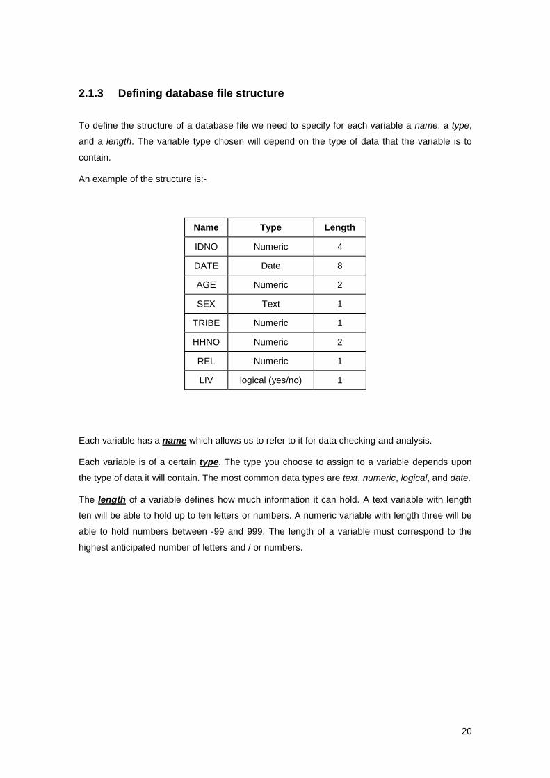
2.1.3 Defining database file structure
To define the structure of a database file we need to specify for each variable a name, a type,
and a length. The variable type chosen will depend on the type of data that the variable is to
contain.
An example of the structure is:-
Name Type Length
IDNO Numeric 4
DATE Date 8
AGE Numeric 2
SEX Text 1
TRIBE Numeric 1
HHNO Numeric 2
REL Numeric 1
LIV logical (yes/no) 1
Each variable has a name which allows us to refer to it for data checking and analysis.
Each variable is of a certain type. The type you choose to assign to a variable depends upon
the type of data it will contain. The most common data types are text, numeric, logical, and date.
The length of a variable defines how much information it can hold. A text variable with length
ten will be able to hold up to ten letters or numbers. A numeric variable with length three will be
able to hold numbers between -99 and 999. The length of a variable must correspond to the
highest anticipated number of letters and / or numbers.
21
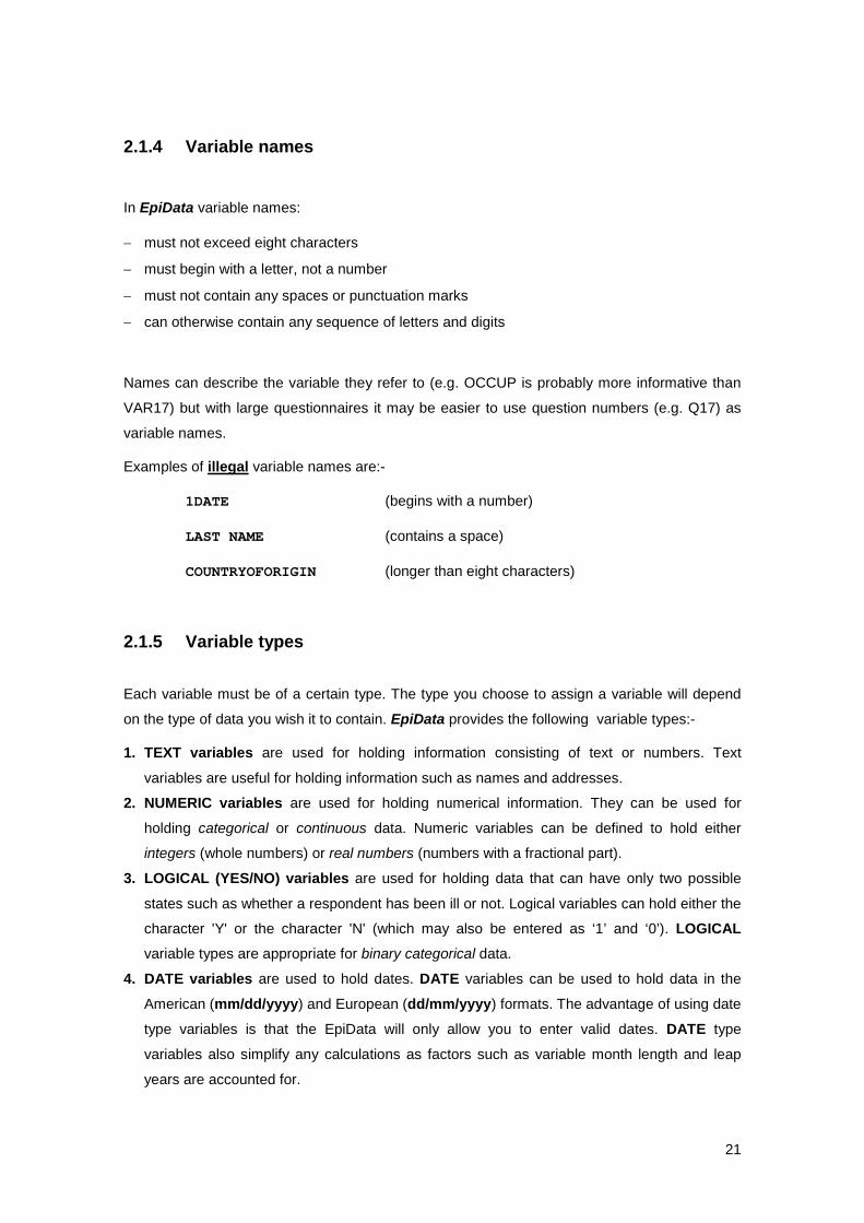
2.1.4 Variable names
In EpiData variable names:
− must not exceed eight characters
− must begin with a letter, not a number
− must not contain any spaces or punctuation marks
− can otherwise contain any sequence of letters and digits
Names can describe the variable they refer to (e.g. OCCUP is probably more informative than
VAR17) but with large questionnaires it may be easier to use question numbers (e.g. Q17) as
variable names.
Examples of illegal variable names are:-
1DATE (begins with a number)
LAST NAME (contains a space)
COUNTRYOFORIGIN (longer than eight characters)
2.1.5 Variable types
Each variable must be of a certain type. The type you choose to assign a variable will depend
on the type of data you wish it to contain. EpiData provides the following variable types:-
1. TEXT variables are used for holding information consisting of text or numbers. Text
variables are useful for holding information such as names and addresses.
2. NUMERIC variables are used for holding numerical information. They can be used for
holding categorical or continuous data. Numeric variables can be defined to hold either
integers (whole numbers) or real numbers (numbers with a fractional part).
3. LOGICAL (YES/NO) variables are used for holding data that can have only two possible
states such as whether a respondent has been ill or not. Logical variables can hold either the
character 'Y' or the character 'N' (which may also be entered as ‘1’ and ‘0’). LOGICAL
variable types are appropriate for binary categorical data.
4. DATE variables are used to hold dates. DATE variables can be used to hold data in the
American (mm/dd/yyyy) and European (dd/mm/yyyy) formats. The advantage of using date
type variables is that the EpiData will only allow you to enter valid dates. DATE type
variables also simplify any calculations as factors such as variable month length and leap
years are accounted for.

22
2.1.6 Null values – missing and not applicable data
Sometimes data items will not be available or are not appropriate to collect for some
respondents (e.g. age at menarche for male respondents). It is important that you take this into
account when designing questionnaires, coding schemes, and data files.
Data that is missing or not appropriate is called null data. There are two types of null data:-
• When data are not available it is defined as missing data. It is generally considered bad
practice to leave data entry spaces on the questionnaire or data entry screen because it can
lead to confusion later. Always consider the codes to use when a value is missing. It is
common practice to use 9, 99, 999 etc. to denote missing data.
• When data are not available because it is not applicable to collect it is defined as not-
applicable. For example, if someone is not married, then the age of their spouse is not
applicable. It is common practice to use 8, 88, 888 etc. to denote not-appropriate data.
Coding not-appropriate data in this way allows you to code data back to missing or null
before analysis.
The coding scheme you decide to use for missing and non-appropriate data must be defined in
advance and consistent across variables.
Any field that is left empty at data-entry or uses missing data in calculations receives a special
missing data code (.). However, it is better to explicitly code missing data as 9,99 etc.

23
2.1.7 Identifying (ID) numbers
When designing a questionnaire or a database file it is important to include a variable that holds
a unique value for each case. This makes finding both paper forms and individual cases in a
database file easier should you need to query or edit a data item. This variable is called the key
or identifier variable.
A survey will often comprise several forms related to one another. The key variable allows
cases in one file to be linked to cases in another file.
Example 1: In this example it is possible to link data from mothers and children using a key
variable (MUMID):
Mother's File Children's File
MumID --- --- --- MumID KidID ---
297 297 001
298 297 002
297 003
298 001
The use of a key variable ensures that data for each mother can be linked with data for that
mother's children. Note that in this example the key variable is unique in the mother's file but not
unique in the children's file. The combination of MUMID and KIDID uniquely identifies each
child.
Example 2: We may wish to link data of cases held in a file with data from a field questionnaire
with data of the same cases held in a file with data from a laboratory report.
A database that consists of more than one linked data file is called a relational database. We
will cover these further in Practical 3.
24
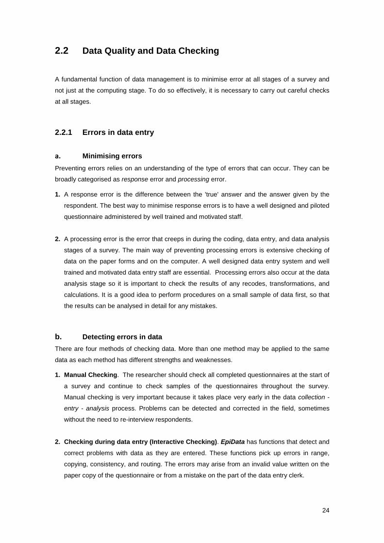
2.2 Data Quality and Data Checking
A fundamental function of data management is to minimise error at all stages of a survey and
not just at the computing stage. To do so effectively, it is necessary to carry out careful checks
at all stages.
2.2.1 Errors in data entry
a. Minimising errors Preventing errors relies on an understanding of the type of errors that can occur. They can be
broadly categorised as response error and processing error.
1. A response error is the difference between the 'true' answer and the answer given by the
respondent. The best way to minimise response errors is to have a well designed and piloted
questionnaire administered by well trained and motivated staff.
2. A processing error is the error that creeps in during the coding, data entry, and data analysis
stages of a survey. The main way of preventing processing errors is extensive checking of
data on the paper forms and on the computer. A well designed data entry system and well
trained and motivated data entry staff are essential. Processing errors also occur at the data
analysis stage so it is important to check the results of any recodes, transformations, and
calculations. It is a good idea to perform procedures on a small sample of data first, so that
the results can be analysed in detail for any mistakes.
b. Detecting errors in data There are four methods of checking data. More than one method may be applied to the same
data as each method has different strengths and weaknesses.
1. Manual Checking. The researcher should check all completed questionnaires at the start of
a survey and continue to check samples of the questionnaires throughout the survey.
Manual checking is very important because it takes place very early in the data collection -
entry - analysis process. Problems can be detected and corrected in the field, sometimes
without the need to re-interview respondents.
2. Checking during data entry (Interactive Checking). EpiData has functions that detect and
correct problems with data as they are entered. These functions pick up errors in range,
copying, consistency, and routing. The errors may arise from an invalid value written on the
paper copy of the questionnaire or from a mistake on the part of the data entry clerk.
25
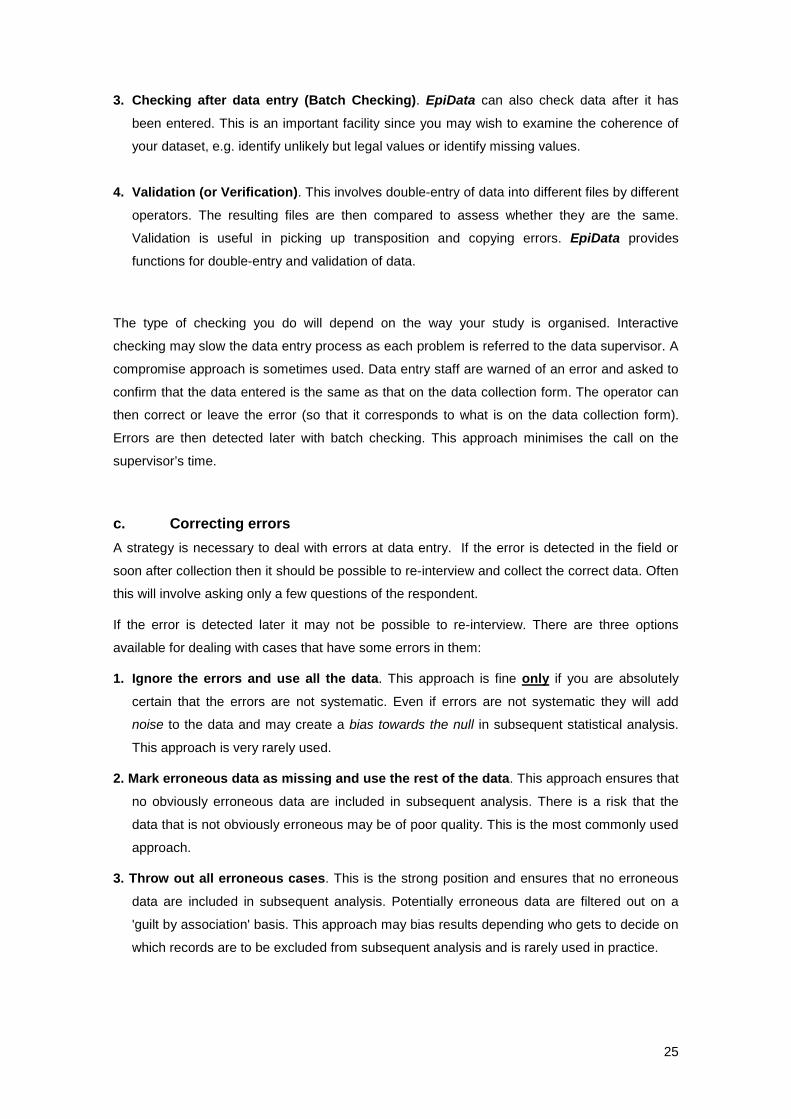
3. Checking after data entry (Batch Checking). EpiData can also check data after it has
been entered. This is an important facility since you may wish to examine the coherence of
your dataset, e.g. identify unlikely but legal values or identify missing values.
4. Validation (or Verification). This involves double-entry of data into different files by different
operators. The resulting files are then compared to assess whether they are the same.
Validation is useful in picking up transposition and copying errors. EpiData provides
functions for double-entry and validation of data.
The type of checking you do will depend on the way your study is organised. Interactive
checking may slow the data entry process as each problem is referred to the data supervisor. A
compromise approach is sometimes used. Data entry staff are warned of an error and asked to
confirm that the data entered is the same as that on the data collection form. The operator can
then correct or leave the error (so that it corresponds to what is on the data collection form).
Errors are then detected later with batch checking. This approach minimises the call on the
supervisor’s time.
c. Correcting errors A strategy is necessary to deal with errors at data entry. If the error is detected in the field or
soon after collection then it should be possible to re-interview and collect the correct data. Often
this will involve asking only a few questions of the respondent.
If the error is detected later it may not be possible to re-interview. There are three options
available for dealing with cases that have some errors in them:
1. Ignore the errors and use all the data. This approach is fine only if you are absolutely
certain that the errors are not systematic. Even if errors are not systematic they will add
noise to the data and may create a bias towards the null in subsequent statistical analysis.
This approach is very rarely used.
2. Mark erroneous data as missing and use the rest of the data. This approach ensures that
no obviously erroneous data are included in subsequent analysis. There is a risk that the
data that is not obviously erroneous may be of poor quality. This is the most commonly used
approach.
3. Throw out all erroneous cases. This is the strong position and ensures that no erroneous
data are included in subsequent analysis. Potentially erroneous data are filtered out on a
'guilt by association' basis. This approach may bias results depending who gets to decide on
which records are to be excluded from subsequent analysis and is rarely used in practice.
26
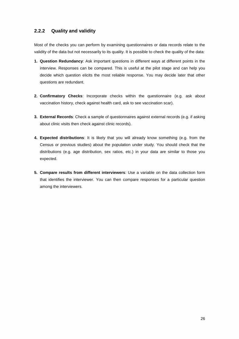
2.2.2 Quality and validity
Most of the checks you can perform by examining questionnaires or data records relate to the
validity of the data but not necessarily to its quality. It is possible to check the quality of the data:
1. Question Redundancy: Ask important questions in different ways at different points in the
interview. Responses can be compared. This is useful at the pilot stage and can help you
decide which question elicits the most reliable response. You may decide later that other
questions are redundant.
2. Confirmatory Checks: Incorporate checks within the questionnaire (e.g. ask about
vaccination history, check against health card, ask to see vaccination scar).
3. External Records: Check a sample of questionnaires against external records (e.g. if asking
about clinic visits then check against clinic records).
4. Expected distributions: It is likely that you will already know something (e.g. from the
Census or previous studies) about the population under study. You should check that the
distributions (e.g. age distribution, sex ratios, etc.) in your data are similar to those you
expected.
5. Compare results from different interviewers: Use a variable on the data collection form
that identifies the interviewer. You can then compare responses for a particular question
among the interviewers.
27
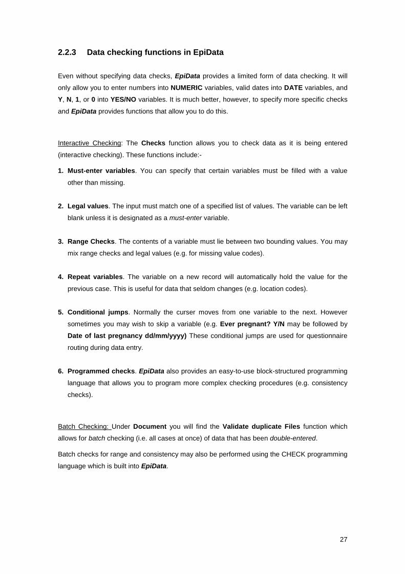
2.2.3 Data checking functions in EpiData
Even without specifying data checks, EpiData provides a limited form of data checking. It will
only allow you to enter numbers into NUMERIC variables, valid dates into DATE variables, and
Y, N, 1, or 0 into YES/NO variables. It is much better, however, to specify more specific checks
and EpiData provides functions that allow you to do this.
Interactive Checking: The Checks function allows you to check data as it is being entered
(interactive checking). These functions include:-
1. Must-enter variables. You can specify that certain variables must be filled with a value
other than missing.
2. Legal values. The input must match one of a specified list of values. The variable can be left
blank unless it is designated as a must-enter variable.
3. Range Checks. The contents of a variable must lie between two bounding values. You may
mix range checks and legal values (e.g. for missing value codes).
4. Repeat variables. The variable on a new record will automatically hold the value for the
previous case. This is useful for data that seldom changes (e.g. location codes).
5. Conditional jumps. Normally the curser moves from one variable to the next. However
sometimes you may wish to skip a variable (e.g. Ever pregnant? Y/N may be followed by
Date of last pregnancy dd/mm/yyyy) These conditional jumps are used for questionnaire
routing during data entry.
6. Programmed checks. EpiData also provides an easy-to-use block-structured programming
language that allows you to program more complex checking procedures (e.g. consistency
checks).
Batch Checking: Under Document you will find the Validate duplicate Files function which
allows for batch checking (i.e. all cases at once) of data that has been double-entered.
Batch checks for range and consistency may also be performed using the CHECK programming
language which is built into EpiData.
28
2.3 The onchocerciasis dataset
Now you will use EpiData to enter baseline data for a trial of an intervention against river
blindness (onchocerciasis) in Sierra Leone in West Africa.
The trial rationale and design are described in the introduction to this unit. Briefly, we will be
looking at a placebo-controlled randomised trial of the effect of the drug ivermectin on infection
with micofilaria. Subjects were enrolled from six villages in Sierra Leone (West Africa), and initial
demographic and parasitological surveys were conducted between June and October 1987.
A questionnaire was used to collect baseline data on the individuals, including demographic and
socio-economic factors, and on subjects' previous experience of onchocerciasis.
Follow-up parasitology and repeated treatment was performed for five further surveys at six
monthly intervals. The principal outcome of interest was the comparison between microfilarial
counts both before and after treatment, and between the two treatment groups. The baseline
questionnaire is shown here. During this practical you will create a data entry form to enter data
from this questionnaire.

29
Onchocerciasis Baseline Survey - Personal Data
IDNO |__|__|__|__|
Name ...............................
Village ...............................
Date of interview DATE |__|__|__|__|__|__|__|__|
Age in years AGE |__|__|
Sex (M or F) SEX |__|
Tribe (Mende 1 Other 2) TRIBE |__|
Household number HHNO |__|__|
Relationship to head of household? REL |__|
1. Self 5. Other Blood Relative
2. Parent 6. Spouse
3. child 7. Other Non-Blood Relative
4. sibling 8. Friend
Have you lived in this village all your life? (Y/N) LIV |__|
How long have you lived in this village? STAY |__|__| (years)
What is your main occupation? OCC |__|
0. None / Missing 5. Office Work
1. At Home 6. Trading
2. At School 7. Housework
3. Farming 8. Mining
4. Fishing

30
2.4 Using EpiData
2.4.1 Starting the EpiData programme
Start EpiData by clicking on the icon in the Statistical Applications window.
The first time you open this, a ‘Welcome’ window will appear. Click on the bottom right box, and
then on ‘Close’ to prevent this window showing again.
EpiData runs in a single window. Functions are selected from menus or from toolbars as in any
other Windows application.
At the top of the screen, there are two toolbars:
Export & backup data
Lists, reports, &c.
Data entry
Add, revise, clear check
Create .REC files
Create .QES files
Code-writer ON / OFF
Pick-list ON /OFF
Preview data form
Paste
Copy
Cut
Undo
Save
Open file
New file
Work process toolbar
Editor toolbar
These toolbars provide shortcuts to the most common EpiData functions. Help is available from
the Help menu. A brief guided tour of EpiData is provided and is available from the Help -> Tour of EpiData menu option. Do NOT run this tour now!
31
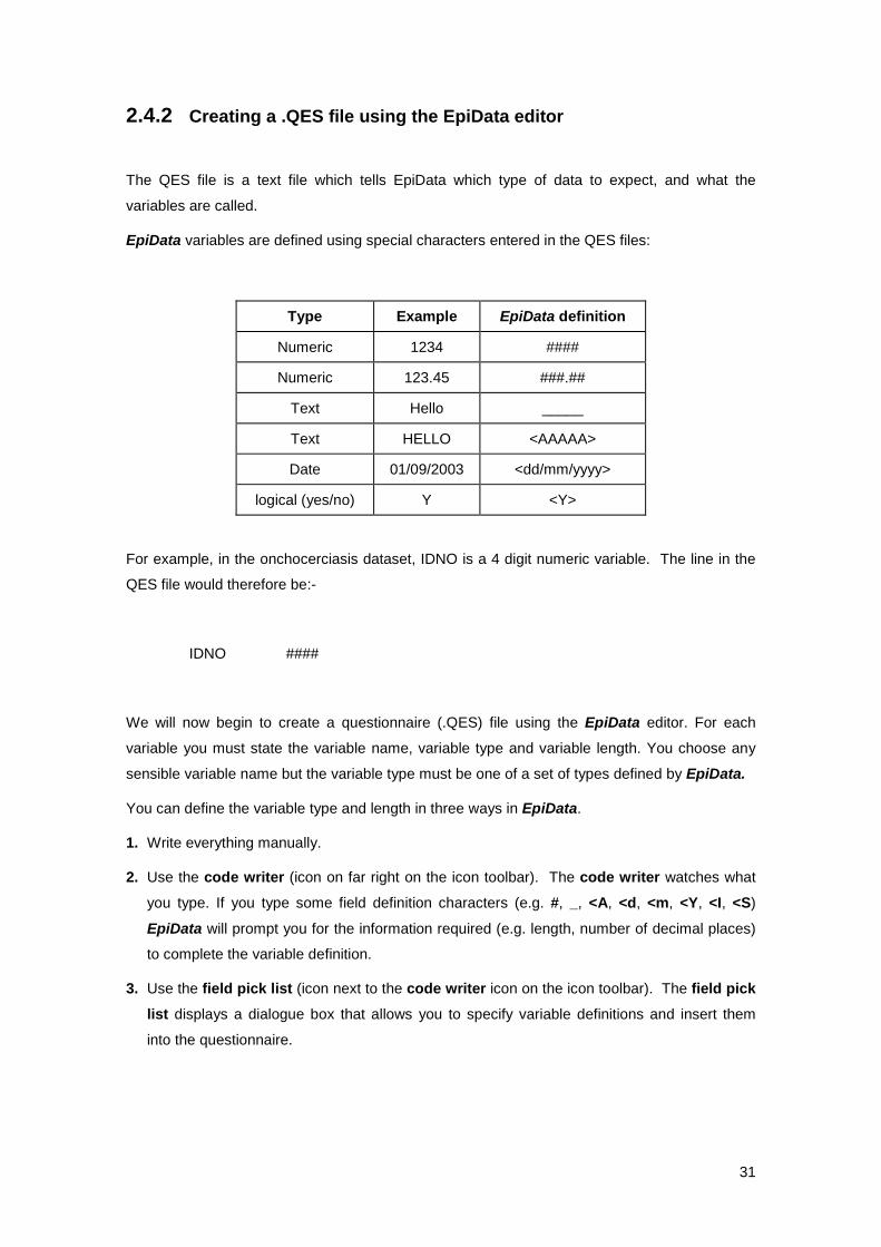
2.4.2 Creating a .QES file using the EpiData editor
The QES file is a text file which tells EpiData which type of data to expect, and what the
variables are called.
EpiData variables are defined using special characters entered in the QES files:
Type Example EpiData definition
Numeric 1234 ####
Numeric 123.45 ###.##
Text Hello _____
Text HELLO <AAAAA>
Date 01/09/2003 <dd/mm/yyyy>
logical (yes/no) Y <Y>
For example, in the onchocerciasis dataset, IDNO is a 4 digit numeric variable. The line in the
QES file would therefore be:-
IDNO ####
We will now begin to create a questionnaire (.QES) file using the EpiData editor. For each
variable you must state the variable name, variable type and variable length. You choose any
sensible variable name but the variable type must be one of a set of types defined by EpiData.
You can define the variable type and length in three ways in EpiData.
1. Write everything manually.
2. Use the code writer (icon on far right on the icon toolbar). The code writer watches what
you type. If you type some field definition characters (e.g. #, _, <A, <d, <m, <Y, <I, <S)
EpiData will prompt you for the information required (e.g. length, number of decimal places)
to complete the variable definition.
3. Use the field pick list (icon next to the code writer icon on the icon toolbar). The field pick list displays a dialogue box that allows you to specify variable definitions and insert them
into the questionnaire.

32
WORKED EXAMPLE: CREATING A NEW QES FILE
- Open EpiData
- Click the Define Data button on the work process toolbar and select the New .QES file option.
This will open a new editor window.
FIRST we will define variables manually.
In the editor window type the following:
IDNO ####
Date of interview <dd/mm/yyyy>
Name ___________________
(this definition allows you to write in any case)
Village <A >
(this definition allows you to write in capital letters only, 12 spaces have been left so village
names of up to 12 letters can be inserted)
Now click on the third icon from the right Preview Data Form of the Editor toolbar to see what
your form looks like for the data entry clerks.
Go back to the editor window by clicking on ‘Untitled 1’ in the bottom left-hand corner of the
screen.
SECOND use the code writer (icon on far right on the icon toolbar).
Turn the code writer on by clicking the code writer icon on the editor toolbar (the icon on the far
right of the toolbar).
Type the entry line for age
Age #
33
When you type # you will see a box asking you to ‘enter length of field’. Age has a maximum of
2 digits, so you enter ‘2’ in the box and click on OK.
You should then see the line
Age ##
in the editor window.
Now type the line entry for Region. You want to record this in capital letters so you type
Region <A
When you type <A you will see a box asking you to ‘enter length of field’. Let’s say that the
longest Region name has eight characters, you enter ‘8’ in the box and click on OK.
You should then see the line
Region <A >
THIRD use the field pick list.
Type the entry line for sex
Sex
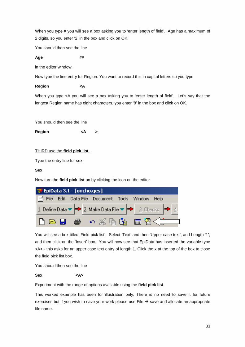
Now turn the field pick list on by clicking the icon on the editor
You will see a box titled ‘Field pick list’. Select ‘Text’ and then ‘Upper case text’, and Length ‘1’,
and then click on the ‘Insert’ box. You will now see that EpiData has inserted the variable type
<A> - this asks for an upper case text entry of length 1. Click the x at the top of the box to close
the field pick list box.
You should then see the line
Sex <A>
Experiment with the range of options available using the field pick list.
This worked example has been for illustration only. There is no need to save it for future
exercises but if you wish to save your work please use File save and allocate an appropriate
file name.

34
It is good practice to create variables with unique, short, easily remembered andmeaningful
names. For long questionnaires it may be easier to use question numbers (e.g. Q01) as variable
names. Complex coding information, while needed on paper collection forms would tend to
clutter up the data entry screen and should not be included.
Exercise 1 – creating a .QES file
Create a .QES file for the onchocerciasis questionnaire (see Section 2.3). You can shorten the
questions to save space.
You should be familiar with three ways of defining variables. During the exercise please
experiment so you find the way that suits you best.
Note : The characters <, >, _, and # are used by EpiData to define variables. Avoid using them
anywhere else in the questionnaire (.QES) file. You should also avoid using the @ character.
2.4.3 Saving the questionnaire (.QES) file
The finished .QES file should look similar to the one below (you may have chosen different
question names)
ID Number ####
Name ______________
Village ______________
Date of Interview <dd/mm/yyyy>
Age in years ##
Sex (M or F) <A>
Tribe (Mende 1, Other 2) #
Household number ##
Relation to head of household? #
Lived in village all your life? <Y>
Years living in this village? ##
What is your main occupation? #
35
Exercise 2 – creating a .QES file
Check your work carefully against the example questionnaire. The variable types should be
identical to those shown, but the questions themselves may be slightly different, depending on
the wording you have chosen.
Save the questionnaire file by clicking the save icon on the editor toolbar or by selecting the
File->Save menu option.
When prompted give the filename oncho.qes and click Save. (You must use the extension
.QES for questionnaire files.)
Make sure you save to the dataepi folder which you should have created! Please ask if you don’t know how to do this.
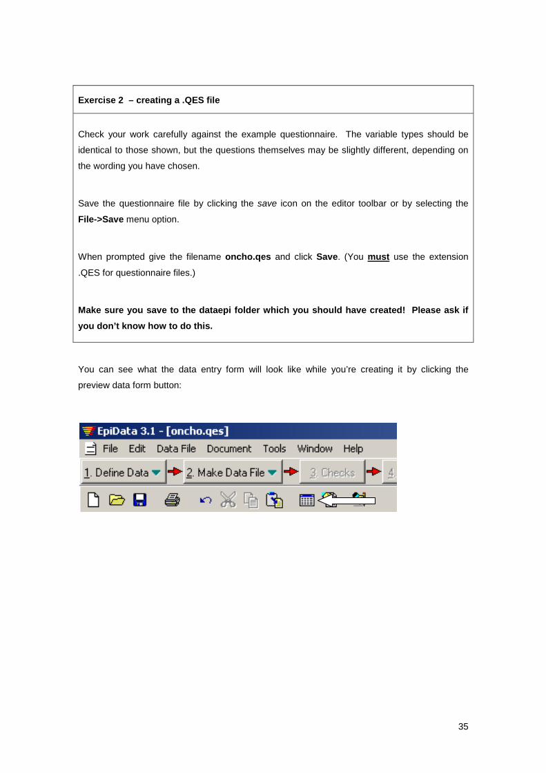
You can see what the data entry form will look like while you’re creating it by clicking the
preview data form button:
36
2.4.4 Creating a data (.REC) file
We will now make a data file so that data can be entered onto the computer.
Exercise 3 – creating a data (.rec) file for the oncho data
Close all the open windows by selecting ‘File’, ‘Close All’ so no more EpiData files are open.
Click the Make Data File button on the work process toolbar.
You will see a box titled ‘Create data file from .QES file’.
In response to ‘Enter name of QES file’, select oncho.qes.
In response to ‘Enter name of data file’ specify oncho.rec (this will be the default)
Click the OK button.
In response to the request for a data file label type Oncho baseline survey.
You will see a box titled ‘Information’ which tells you that the file oncho.rec has been created.
Click OK
EpiData has now created a data file oncho.rec using the information contained in the .QES file
(oncho.qes).

37
You have now completed the process:-
and can now enter data that will be stored in the data (.REC) file.
Text editor
.QES file
Make data file function
.REC file
Defines the structure of the data file and the layout of the data entry form.
Holds the data
38
2.4.5 Entering data
You are now ready to enter data from the baseline onchocerciasis survey.
Exercise 4 – entering and saving data into the .rec file
Click the Enter Data button on the work process toolbar (option 4).
Specify the file oncho.rec and click the Open button.
EpiData will display the data entry form for oncho.rec ready to receive data.
Enter the data from the 6 questionnaires in Appendix 3.
Missing data should be left blank for now.
After you have entered all the data for one case (record), you will see the message Save record to disk?
Click the Yes button or press return.
A new (blank) data form will be displayed. Note that the text New/1 is displayed in the lower
right corner of the EpiData window.
Enter data for all of the 6 sample cases, writing each to disk.
2.4.5.1 Notes on entering data
• Note that you can only enter the type of data shown on the status bar at the bottom of the
EpiData window. This depends on the variable types you specified in the questionnaire
(.QES) file. If you enter data of the wrong type into a variable (or an invalid date into a DATE
type variable) then EpiData will warn you. Re-enter the correct data.
• Pressing the return key on its own (i.e. entering no data) will set a variable to 'missing'. This
is a special value that is recognised as missing by EpiData. Statistical and database
packages vary in the way they treat missing data so it may be best to use explicit codes for
missing and not-available data which will have to be recoded before data can be analysed.
• You may need to press return to move onto the next variable if the data you enter does not
completely fill a particular variable.
• The ↑ and ↓ keys allow you to move between variables. The CTRL+HOME keys will move
the cursor to the first variable. The CTRL+END keys will move the cursor to the last variable.

39
Data can also be edited after it has been saved to disk.
The data controls:
Control Function
Display first record in the data file
Display previous record in the data file
Display next record in the data file
Display last record in the data file
Display a new blank record ready to receive data
Mark the currently displayed record for deletion
At the bottom of the screen is a means of moving from case to case within a data file. These
functions are also available on the Goto menu and also have keyboard shortcuts.
Exercise 4 continued – making changes to the .rec file
Use the keys in the table above to review the cases that have been entered.
Change the missing value (occupation for ID 1601) to be coded as 9
Save the edited case by clicking the Yes button when asked to Save record to disk? You will
also see this prompt if you change any data and move to a different record or a new blank
record before saving the changed data.
If you wanted to enter more data, you can display a new blank record by pressing CTRL+ N.
EpiData provides several different ways of accessing the same function. For example, the
function to display a new blank record can be accessed using the menus Goto New Record,
using a keyboard shortcut CTRL+N, or by clicking the relevant data control. Use the method you
feel most comfortable with.

40
2.4.6 Variables names
Exercise 5 – finding variable names within a .rec file
From within the data entry window, click on Goto -> Find Field.
The dialogue box displays variable names that EpiData has automatically assigned to each
variable. It does this by using the first eight non-blank characters of text for each variable.
Some words such as ‘what’, ‘are’, and ‘of’ are discarded automatically (e.g. Date of
interview becomes DATEINTERV). These are the variable names used in the analysis.
However, you may wish to rename these variable (field) names.
Exercise 5 continued – renaming variables
Close the dialogue box and data entry form
Now choose the ‘Tools – Rename fields’ option.
Select oncho.rec. In the right hand column of the dialogue box type in the following new field
names.
IDNO, DATE, AGE, SEX, TRIBE, HHNO, REL, LIV, YEARS, OCC.
Save these revised variable names by clicking ‘Save and close’. You will see an Information
box confirming that the names have been changed.
Go to the Oncho.REC file again using the Enter Data tab and look check that the field names
have been altered (you can use the Goto menu or you could just press F4).

41
2.4.7 Finding records
Exercise 5 continued – finding specific records within the .rec file
Open the revised file oncho.rec using the Enter Data tab.
Decide which variable you want to search on. In this case we will search using the variable
Household number.
EITHER
Place the cursor in the box by the variable Household number.
OR
Press the F4 key which will show a box with all variable names. Double-click on HHNO
Close the box by clicking on the top right hand square.
Press CTRL + F (or GOTO –> FIND RECORD) to display the Find record dialogue box.
If you want to find all records with HHNO=8, type 8 in the criteria box next to HHNO and click
OK. This closes the Find record dialogue box, leaving open the record file displaying the
records with HHNO=8.
You move among these specified records using the F3 key or Goto -> Find Again.
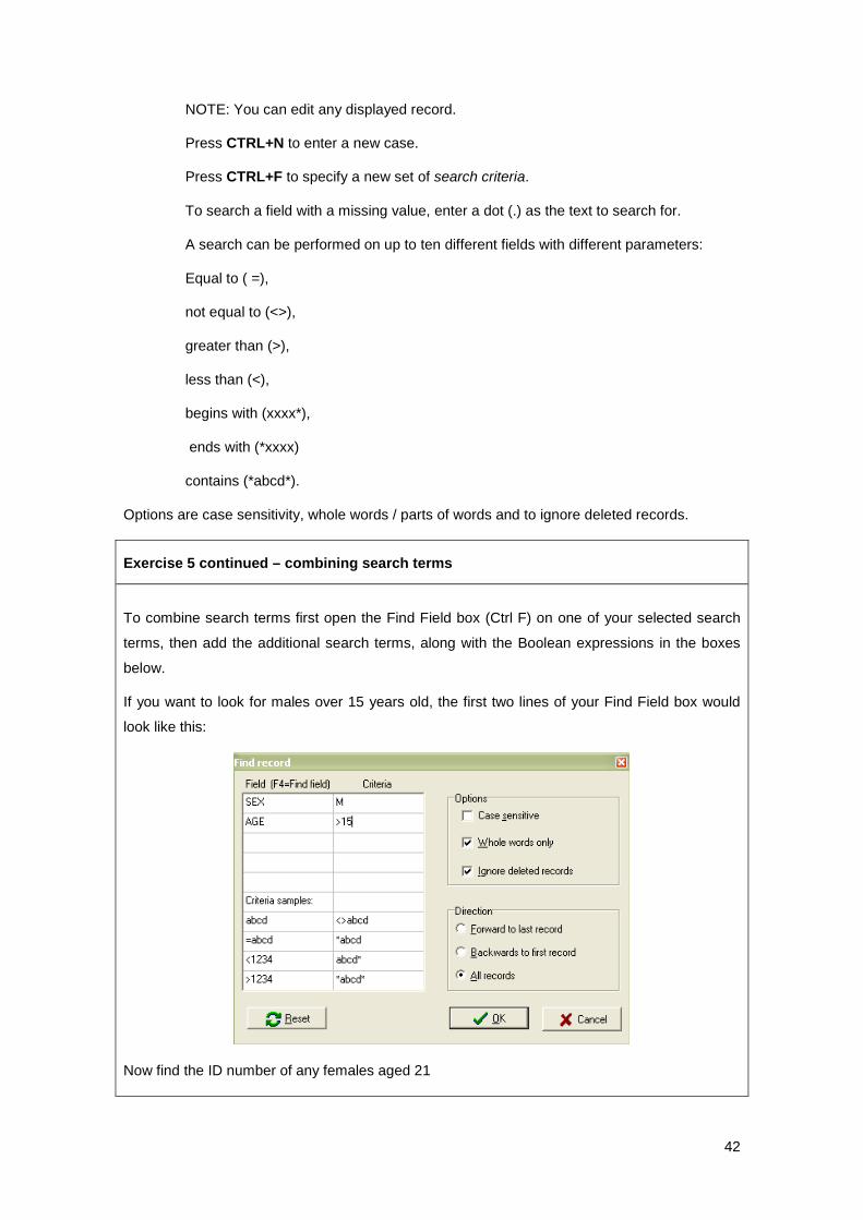
42
NOTE: You can edit any displayed record.
Press CTRL+N to enter a new case.
Press CTRL+F to specify a new set of search criteria.
To search a field with a missing value, enter a dot (.) as the text to search for.
A search can be performed on up to ten different fields with different parameters:
Equal to ( =),
not equal to (<>),
greater than (>),
less than (<),
begins with (xxxx*),
ends with (*xxxx)
contains (*abcd*).
Options are case sensitivity, whole words / parts of words and to ignore deleted records.
Exercise 5 continued – combining search terms
To combine search terms first open the Find Field box (Ctrl F) on one of your selected search
terms, then add the additional search terms, along with the Boolean expressions in the boxes
below.
If you want to look for males over 15 years old, the first two lines of your Find Field box would
look like this:
Now find the ID number of any females aged 21

43
Close the oncho.rec data entry form.
2.4.8 Summary so far
Creating a database file in EpiData is a two stage process:
1. First you use the text editor to create a screen questionnaire, or data entry form. This must
include the variable names, types, and lengths. A questionnaire file must have the extension
.QES. EpiData allows you to preview the data-entry form before saving the questionnaire
(.QES) file and making a data (.REC) file.
2. The structure of this .QES file in turn defines the structure of the data file. In EpiData a data
file is called a record file and has the extension .REC.
The questionnaire (.QES) file defines the structure of the record (.REC) file and the layout of the
data-entry form. Data are entered and stored in the record (.REC) file.
The Make data file function is used to create a record (.REC) file from a questionnaire (.QES)
file.
The Enter data function is used to open and to enter data into an existing record (.REC) file.
Text editor
.QES file
Make data file function
.REC file
Defines the structure of the data file and the layout of the data entry
form.
Holds the data

44

45
Data Management using EpiData and Stata
Practical 1 : Questionnaire Design
Objectives of this session
The objective of this session is to develop skills in questionnaire design. By the end of this
session you will have:-
• had practice at constructing a questionnaire comprising clear questions.
• become aware of the manner and purpose of piloting questions and of acquiring
informed consent.
• understood the importance of high standards in quality control and ethics and how
to ensure that these are maintained.
In this practical you should work in groups of 5-6.
Please read all the notes on questionnaire design in Session 1 before you start constructing the questionnaire.
The task for each group is to design a short questionnaire to investigate risk factors for flu among
LSHTM students, using a cross-sectional study. Assume that the questionnaire will be
administered in March 2012 and should ask about flu during winter of 2011/2012.
Flu is a viral infectious disease of the upper air passages. The symptoms are:-
• fever that comes on quickly (38 – 40 C; 100 – 104 F)
• sweating and feeling feverish· General muscle aches and pains
• a feeling of general tiredness
• dry, chesty cough
• sneezing
• running or blocked nose
• difficulty sleeping
The hypothesis you want to test is that mode of transport influences risk of contracting flu in London.
Continued overleaf…

46
You have to decide how to ascertain information about the outcome, risk factors and potential
confounders. Confine your questionnaire to a maximum of 10 questions, and write these on a
transparency. Take care over the layout of the questionnaire, and the categories for responses.
After one hour, each group will show their questionnaire to the other groups in the room.
Discuss the similarities and differences of each groups’ questionnaires, and the problems you
encountered in constructing the questionnaire

47
2.5 Adding checks in EpiData
For each variable you can specify certain restrictions on data entry. You can do this either by
using the drop-down menu or by typing the restriction manually. You will learn how to use both
methods.
We will add some checks to the data entry system for the Onchocerciasis data.
Exercise 6 : Opening the CHK file
Close any open windows, and then click the 3. Checks button Select the file oncho.rec and click the Open button.
The data-entry form appears, as well as the following dialogue box which allows you to specify
data checking rules. First make sure that the variable you are interested in is displayed at the
top of the check box. You can change your choice of variable using the drop-down menu at the
top of the chk box.

48
Each dialogue box has a different function and we explain these below.
Range,
Legal
Specifies what values may be entered, e.g. [1] for a numerical variable 1-4,9
specifies that only values 1,2, 3, 4 and 9 may be entered. [2] M,F specifies that
only the letters M and F may be entered
Jumps Specifies that if a certain value is entered in this variable, the cursor jumps
automatically to another variable, e.g. Y>OCC specifies that if you enter Y for
the selected variable, the cursor will jump automatically to variable OCC
Must enter Specifies whether or not there may be missing values for the selected variable.
Use the drop-down arrow to select Yes or No. Any essential fields should
have the ‘Must enter’ check.
Repeat This check is useful when almost all respondents have the same value for the
selected variable. This becomes the default value but you can change it when
entering data for a respondent with a different value.
Value label You may wish to label the values you use for a variable, especially when they
are not self-explanatory. Consider carefully whether a variable needs a value
label. In general, labels are given to values of a categorical variable. You can
edit the labels by clicking on the + box to the right of the dialogue box. This will
open the ‘Edit values label’ box in which the first and last line of the text needed
to label the values of the selected variable is given LABEL label_VAR END
Place your cursor at the end of the first line and press enter. Insert the labels for
legal values, for example LABEL label_VAR 1 Self 2 Spouse 3 “Any Other” END
Where a value label has more than one word you must insert the double inverted
commas “xx xx”. When you have finished writing text in the Edit value labels box, you must click
on Accept and close.
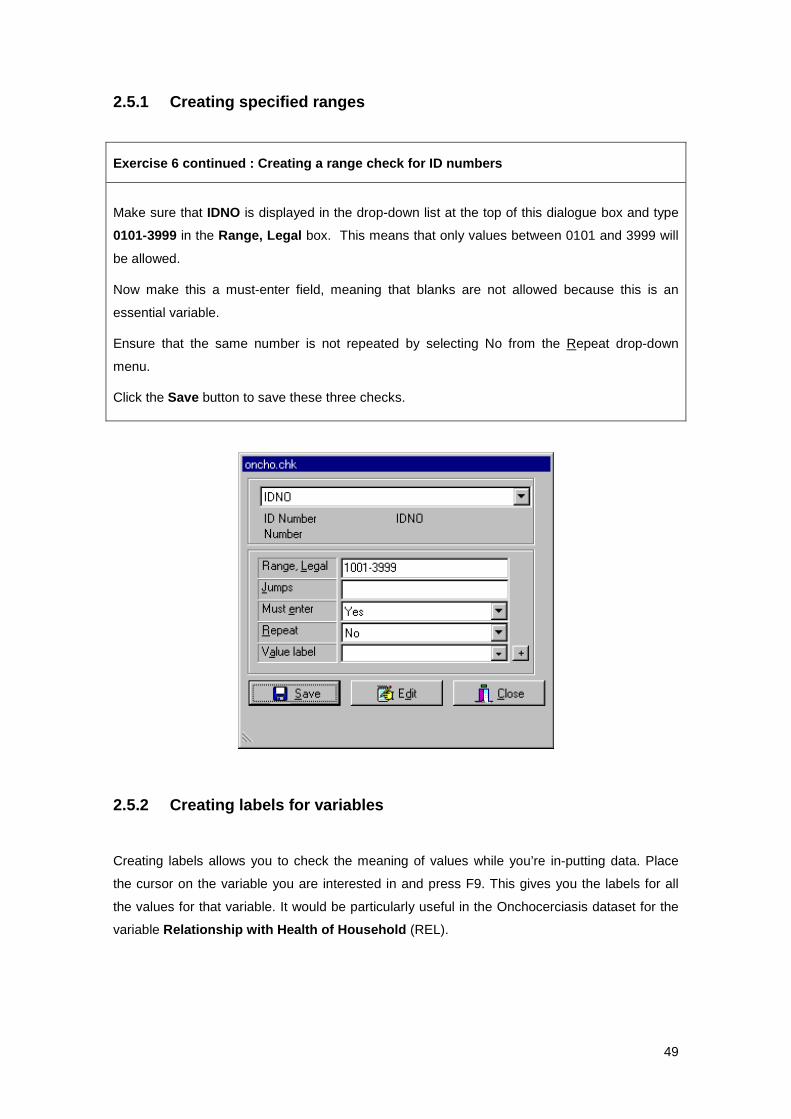
49
2.5.1 Creating specified ranges
Exercise 6 continued : Creating a range check for ID numbers
Make sure that IDNO is displayed in the drop-down list at the top of this dialogue box and type
0101-3999 in the Range, Legal box. This means that only values between 0101 and 3999 will
be allowed.
Now make this a must-enter field, meaning that blanks are not allowed because this is an
essential variable.
Ensure that the same number is not repeated by selecting No from the Repeat drop-down
menu.
Click the Save button to save these three checks.
2.5.2 Creating labels for variables
Creating labels allows you to check the meaning of values while you’re in-putting data. Place
the cursor on the variable you are interested in and press F9. This gives you the labels for all
the values for that variable. It would be particularly useful in the Onchocerciasis dataset for the
variable Relationship with Health of Household (REL).

50
Exercise 7 : Creating labels for the variable SEX
Create labels for the legal values of the variable SEX: M for Male and F for Female.
Hint: Follow the pattern specified in the table above (section 2.5.) to label the values of the
variable SEX.
Click the Accept and Close menu option.
Note that the Value label box now contains the name of the value and label set label_sex.
You can use this value label for other variables (e.g. if you had a variable ‘sex of child’)
Save the change by clicking on the Save icon.
Note that when a value label consists of more than one word, it must be enclosed in double
quotes (e.g. "No data”).

51
2.5.3 Setting up checks We will now set up some further interactive checks for data entry.
Exercise 8 : Further range and legal value checks for the onchocerciasis data
Use the oncho.chk box to set up the following checks.
1. Restrict AGE to 12 to 70 years and 99 (for missing)
2. Label the value 99 as missing for this variable.
3. Label the values for the variable Tribe. Since most people in the survey are of the Mende
tribe, set the ‘Repeat’ option to ‘Yes’.
4. For variable HHNO specify a range of 1 to 39, and allow the entry of 99 for missing data.
5. Select the REL variable and specify the value and label set outlinedpn page 31.
Hint: remember to use the inverted commas “xx” when a label has more than one word.
Accept and close the Edit value labels box.
6. Select the LIV variable. Using the Jumps box, specify that if a value of Y is entered, the
cursor will jump automatically to the OCC variable.
7. Label the values for the variable OCC outlined on page 32.
When you have specified all these checks, save them using the Save button and then click the Close button to close the Check window.
Exercise 9 : Entering data after creating checks
Open the oncho.rec file. (Hint: use the 4.Enter Data menu)
Try entering some data (make some up) to verify that the must-enter, repeat, range, legal value,
and jumps checks that you specified work correctly.
Note that you can use the F9 or + key to display value and label sets.
If your checks do not work as expected then close the data entry form and from the drop-down
toolbar use Checks -> Add / Revise to edit your checks. Enter some more data into oncho.rec
and verify that the checks work correctly.
Close the data entry form when you are satisfied that your checks are working as expected.
2.5.4 Specifying a KEY UNIQUE variable 1 1 Self, 2 Parent, 3 Child, 4 Sibling, 5 Other blood, 6 Spouse, 7 Other non blood, 8 Friend, 9 Other. 2 1 At home, At school, 3 Farming, 4 Fishing, 5 Office work, 6 Trading, 7 Housework, 8, Mining, 9 Other.

52
EpiData provides a way of ensuring that a variable is unique (i.e. that no other case has the
same value in a particular variable). This is useful because it speeds up searches for data and
ensures a measure of data integrity as it makes it difficult for the same person's data to be
entered twice.
Exercise 10 : Making ID number a key unique variable
Not all checks are available on easy drop-down menus. To stipulate a key unique variable we
have to write the text ourselves.
Open the oncho.chk file using the 3.Checks tab and opening the file oncho.rec.
Move the cursor to the IDNO variable and click the Edit button to open the Edit checks for this field box.
EpiData displays the CHECK commands associated with this variable:
IDNO
RANGE 0101 3999
MUSTENTER
END
We will now alter the CHECK command to stop us entering duplicate values of IDNO
Edit the CHECK commands associated with this variable to read:
IDNO
KEY UNIQUE
RANGE 0101 3999
MUSTENTER
END
You must click the Accept and Close menu option (same as with the Edit Value Labels box).
Click the Save button to save the checks and then click the Close button.
Go to ‘Enter data’ and enter data for ID 0801. Make sense of what happens.
Close the data entry form.

53
It is good practice to use the KEY UNIQUE option for the identifying variable to prevent errors in
data entry.
When you use the KEY UNIQUE command a new file with the same name as the record (.REC)
file but with the extension .EIX is created. This index file speeds up the way EpiData searches
for data.
2.5.5 Limitations of interactive data checking
EpiData provides very powerful functions for interactive data checking. Interactive checking is
good at dealing with many sorts of error but cannot provide a complete shield against typing
errors and digit transposition (e.g. 3 and 4 may both be valid occupation codes, 23 and 32 may
both be valid ages). Also, data may be invalid on the data collection form and EpiData may not
allow the data to be entered. This can slow the data entry process as each problematic case
may need to be checked by the data supervisor as it is entered.
Another problem with interactive checking is that it is prescriptive. It does not allow any data that
violate the data checking rules to be entered. This means that interactive checking is best used
when there can be no controversial-but-correct (i.e. real-but-unlikely) values.
EpiData provides another method of data checking called validation. Validation involves data
being entered twice into two separate files by two different data entry operators. The two files
are then compared and any discrepancies can be checked against data collection forms.
With validation it is important that the data are entered by two different operators. This is to
overcome errors caused by digit preferences (the same operator will tend to make the same
mistakes in the same situations).
Validation works well when each case has a key or unique identifier variable (specified using
KEY UNIQUE in the check (.CHK) file). If a key variable is not used then data must be entered
into the two files in the same order. This is difficult to guarantee so always use a key or unique
identifier variable.

54
2.6 Double entry and validation We will first create two new data files and set up data checking rules. EpiData makes this easy
by providing functions specifically designed to help you do this.
The process is shown below
Exercise 11 : creating a duplicate file called oncho_a.rec
Close any open editor windows and data entry forms and select the Tools -> Copy Structure
menu option.
Select the file oncho.rec and click the Open button. The Copy File Structure box will open.
In the text box labelled File name type oncho_a.rec
Tick the Copy check file option and click the OK button.
This will create an empty data file called oncho_a.rec with exactly the same structure as
oncho.rec and also create a file called oncho_a.chk which contains the data checks that you
specified for oncho.rec. Epidata will inform you that the files have been copied. Click the OK
button.
Start Continue
Enter / edit data
in ONCHO.REC Validate
Enter / edit data
in ONCHO_a.REC
Yes, differences exist
Yes, differences exist
N Any difference
?
55
Exercise 12: entering data into the file oncho_a.rec
Enter the following data into the oncho_a.rec data file:
IDNO DATE AGE SEX TRIBE HHNO REL LVILL STAY OCC
0801 19/09/1987 35 M 1 08 1 N 24 8
0802 18/09/1987 31 F 2 08 6 N 25 5
1601 19/11/1997 18 F 2 16 8 Y 9
0803 18/09/1987 21 F 1 08 4 Y 5
1001 29/10/1987 15 M 2 10 3 Y 2
1002 29/10/1987 45 M 1 10 1 N 20 2
Close the data entry form when you have entered all five cases. Note that if the response to LIV is
‘Y’, then EpiData automatically jumps to OCC. This is because if someone has lived in the village
all of their life, and we know their age, we already know how many years they have lived there.
Close the data entry form. (File -> Close form)
We are now going to compare the files oncho.rec and oncho_a.rec to identify differences
between them.
Exercise 13 : Comparing two databases to identify errors in data entry
Select Document -> Validate Duplicate Files menu item. In response to the prompts for the
names of the two files specify (you can type the filenames or select from a file browser by clicking
the folder icon next to the entry boxes) the files oncho.rec and oncho_a.rec and click the OK
button.
You must tell EpiData to compare records that have the same identity number. Click the box next
to IDNO to identify it as the key field (i.e. the field that will be used to identify the records in each file
that ‘belong’ to each other) and click the OK button.
EpiData responds with a list of discrepancies (by IDNO) between the two files displayed in an
editor window. The list is a text file which you can edit, save, or print.
Print the file or make a note of the reported discrepancies. Close the editor window. Check the
discrepancies against the original questionnaire (Appendix 3), and edit the rec files until they are
both correct. Check using Document -> Validate Files again to compare the two files again.

56
To ensure good quality data you should use both interactive checking and validation.
Double entry may seem an unnecessary step that adds time and expense to a study but it is an
essential step to ensure data quality and should always be used. Some researchers hold the
view that errors in data are random events and will not lead to bias in large studies. This is a
mistaken view as many typing mistakes are caused by a systematic digit preference by the data
entry operator and can lead to a systematic bias in the data.
2.7. Exporting data from EpiData
Once you are satisfied that your data are of good quality, it is time to export the dataset to a
programme suitable for analysis.
2.7.1 The Onchocerciasis dataset
In the Onchocerciasis dataset we have data from several sources:
Each person has one demographic record
Each person has one or more microfilariae count records
Each person has one or more blood results records
Each person has one treatment code record
Demography[1]
Microfilariae counts[1 or more]
Blood results[1 or more]
Treatment[1]
57
Demographic questionnaires were filed by IDNO in the field office. The data entry task was
simplified by entering data into three separate files for IDNOs 1-999, 1000-1999 and 2000+. The
same questionnaire (.QES) file was used and the end result was three different files of exactly
the same structure (demog_1.rec, demog_2.rec, and demog_3.rec).
Six files were used to store the data:
Filename Contents
demog_1.rec Baseline demography file
demog_2.rec Baseline demography file
demog_3.rec Baseline demography file
blood.rec Blood results
micro.rec Microfilariae counts
tmtcodes.rec Randomisation codes (drug or placebo)
We are going to combine baseline demographic data with laboratory data and treatment codes,
to answer the question of whether the drug ivermectin was associated with a lower prevalence
of microfilaria at round 5. We will use Stata12 for this, so the first step is to export data from
EpiData into Stata.
2.7.2 Exporting data to Stata
EpiData provides a set of functions that allow you to export data in a variety of common file
formats (text, Stata, dBase III, Excel, SPSS, SAS). All of these functions are available from the
Export Data menu.
Exercise 14: Exporting data from EpiData to Stata
Open Epidata 3,1 and use the Export data option to export the demog1.rec file to Stata 12.
You do this by clicking on
Export Data, Stata, and select demog_1.rec.

58
Stata uses lower case variables for names, so ensure that the ‘lower case’ is selected under the
Options tab.
Please make sure that you have created the folder
h:\dataepi
… and exported the data to that folder.
Repeat for the remaining 5 files in the box above.
All your data on this course should be saved in the folder you have created called DataEpi so
please export the Onchocerciasis files to that folder.
Open Stata12 and check that the folders have been exported correctly
2.7.3. Folder management in Stata
In Stata, it is good practice to first define the default folder where you save your material. You
can do this using the ‘cd’ (change directory) command. This means that all files you create will
be stored in this directory.
Exercise 15.
Open Stata and change directory to the one containing your data management files by typing:
cd h:\dataepi
use demog_1.dta
Use the describe command to check that all the variables are there

59
Data Management using EpiData and Stata
Practical 3 : Data Management using Stata 12
I : Basics
Objectives of this session
After data has been entered and checked, there are two main tasks of data management –
manipulating datasets to create useful combinations which can be used in analysis, and data
housekeeping – for example: labelling values, dealing with missing values, creating new
variables. These are all essential commands that you need to know to use Stata for data
analysis.
By the end of this session you should be able to:-
• Use Stata ‘do’ files appropriately
• Create and transform variables
• Join datasets using ‘append’
• Label variable names and values
• Know the difference between ‘recode’ and ‘replace’
• Generate new variables using the ‘egen’ command.
3.1. Introduction
Following on from the practical last week, you should have the following six Stata datasets in
the folder h:\dataepi :-
Filename Contents demog_1.dta Baseline demography file 1 demog_2.dta Baseline demography file 2 demog_3.dta Baseline demography file 3 blood.dta Blood results micro.dta Microfilariae counts tmtcodes.dta Randomisation codes (drug or placebo)
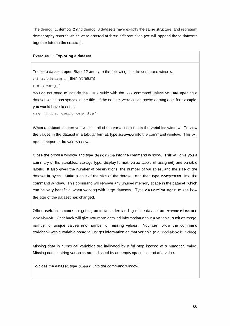
60
The demog_1, demog_2 and demog_3 datasets have exactly the same structure, and represent
demography records which were entered at three different sites (we will append these datasets
together later in the session).
Exercise 1 : Exploring a dataset
To use a dataset, open Stata 12 and type the following into the command window:-
cd h:\dataepi (then hit return)
use demog_1
You do not need to include the .dta suffix with the use command unless you are opening a
dataset which has spaces in the title. If the dataset were called oncho demog one, for example,
you would have to enter:-
use “oncho demog one.dta”
When a dataset is open you will see all of the variables listed in the variables window. To view
the values in the dataset in a tabular format, type browse into the command window. This will
open a separate browse window.
Close the browse window and type describe into the command window. This will give you a
summary of the variables, storage type, display format, value labels (if assigned) and variable
labels. It also gives the number of observations, the number of variables, and the size of the
dataset in bytes. Make a note of the size of the dataset, and then type compress into the
command window. This command will remove any unused memory space in the dataset, which
can be very beneficial when working with large datasets. Type describe again to see how
the size of the dataset has changed.
Other useful commands for getting an initial understanding of the dataset are summarize and
codebook. Codebook will give you more detailed information about a variable, such as range,
number of unique values and number of missing values. You can follow the command
codebook with a variable name to just get information on that variable (e.g. codebook idno)
Missing data in numerical variables are indicated by a full-stop instead of a numerical value.
Missing data in string variables are indicated by an empty space instead of a value.
To close the dataset, type clear into the command window.

61
3.2 When to save and when to clear?
When you open an existing Stata dataset, a copy of that dataset is taken from the computer
hard drive and placed into memory. Any changes which you then make to that dataset will not
be saved unless you deliberately use the save command. To save a dataset under a new
name, type save [newdatasetname]. To replace an existing dataset with an updated
version, type save [existingdatasetname], replace.
When you type clear without saving the open dataset will be removed from the computer
memory and any changes you have made will be lost. This can be useful if you are
experimenting with a dataset and don’t wish to make any permanent changes.
If you open a dataset, make some changes and then try to open another dataset without typing
clear first, you may get the following error message (in red text):-
no; data in memory would be lost
This is to warn you that you will lose the changes that you have made to your original dataset.
Either save the original dataset using the save command, or type clear to remove the
original dataset from memory.
3.3 “Do” files
3.3.1 What is a do-file?
In the exercise above you have used Stata interactively, in that you enter your commands one
at a time into the command window, and obtain the results of each command immediately after
entering the command and before submitting the next command.
However, when carrying out an analysis it is essential to create a programme file (called a do-
file) which contains all your commands. If you want to run a set of commands more than once
you can just run the do-file instead of typing all the commands again. Stata includes a ‘do-file
editor’ which you can use to create, save and edit do-files.
To create a new do-file, click the do file editor button on the Stata toolbar, located at the top left
of the screen.
Do file editor
62
Clicking the do-file editor button opens a separate text editor window, into which you can directly
write your Stata commands. Use the Save button to save your file and the Execute (do) button
to run the entire programme. You can also run just part of a do file by highlighting the text you
want to run before clicking the Execute (do) button.
A new .do file editor window
If you want to open a do-file that you saved and closed earlier, just click on the do-file editor
icon, then click the open (yellow folder) button within the do-file editor screen to get a list of
existing do-files.
Stata executes the commands of the programme you have created in your do-file sequentially,
sending output to the screen, until it reaches the end of the programme contained in the do-file.
By default, Stata will stop executing the commands if it encounters an error. You can check that
this has not happened by making sure that there are no error messages in red text immediately
prior to the do-file finishing.
You must specify the path-name if the do-file is in a folder other than that in which you are
working. Alternatively you can change the default folder.
3.3.2. Comments in do files
It is good practice to add comments to your do files to explain what the programme is doing.
This helps you to understand a programme quickly if you return to it a long time after you first
wrote it, and helps others to understand what a programme does if it is made available to them.
In Stata versions 11 and 12 (but not in earlier versions) comments appear in the do-file in green
so that they are easy to distinguish from the actual programme.
Execute (do) button Save button
63
The simplest way of creating a comment is to start a line with * . So for example, the line:-
* read in the dataset
Would be treated as a comment and ignored. You would then want to follow the comment with an actual command, such as:-
* read in the dataset
clear
use demog_1
which would clear Stata’s memory and open the demog_1 dataset.
For longer comments which run over several lines, it can be useful to use the following syntax:-
/* Comment line 1 Comment line 2 Comment line 3 */ Any text between /* and */ is interpreted as a comment, no matter how many lines separate them.
3.3.3 The “Set more off” command
A useful command to put at the top of a do-file is
set more off
By default, Stata stops output from your do-file when the results screen is full and displays in blue the message –more- . You must press the return key to continue the output. The command set more off tells Stata not to display the -more- message and, therefore, not to pause while the do-file is running.

64
3.3.4 A do-file template
A useful template for a do file, with introductory comments about the location/purpose of the file, changing the folder location and opening a dataset, is as follows:-
/* Name of project Purpose of do-file Who wrote it When it was written Where it is */ clear set more off cd [path] use [datasetname]
Exercise 2 : Creating a do file
Create a do file following the template above which will open the dataset demog_1.dta Save the do file as demog_1.do
3.4 The Display command
You can also use display to perform calculations, using display [ expression], where expression
can be an equation or some function. Below are two examples , with the resulting Stata output.
display (45.6*17.6)/34.3 23.398251 display sqrt(54.6) 7.3891813
65
3.5 Log files
The log file is a record of your commands AND OF ALL YOUR DATA OUTPUT, and can be a
valuable record of how a do file changes and analyses your data.
When writing a do file, include the command
log using [filename], replace at the top of your do file, and
log close at the end
where [filename] is the name that you choose to give to the log file.
This saves your file in the .scml format, which is read using the Stata viewer. If you wish to
save your log files as text (.txt) files, then specify this file type when opening the log, so that the
opening line would be
log using [filename].txt, replace
Note that the replace command will over-write the contents of any existing file with the same
filename. If you wish to preserve previous log output, choose a different file name for the new
log.
There is always a risk when using a do file that a mistake has been made and that the
programme will stop running before the end, i.e. before your ‘log close’ command. You may use
the cap log close command before opening the log file, to instruct Stata to close the log
file automatically if there is an error in the do-file and it doesn’t reach the end of the programme.
Exercise 3 : Creating a do file continued
Amend your do-file to include creation of a log file. Remember to close the log file at the end of
the do-file.

66
3.6 Appending Data
Appending datasets describes the process of joining individual datasets together “end to end”
into a single dataset. In this case, all three of our demog files contain the same baseline
demographic data for different individuals from the Onchocerciasis study. We want to join these
three files end to end, to create a single file containing records for all individuals in the study.
Where the individual datasets contain variables of the same name and type, Stata will append
these together so that the data in these variables simply follow-on from each other. In the
illustration below, the idno and age variables from demog_1.dta and demog_2.dta are shown,
with the first five records from each dataset. These datasets contain the same variable names,
and so when they are appended together the variables with the same name are appended.
Original dataset
Original dataset
demog_1.dta demog_2.dta
idno age idno Age
1 62 1001 73
2 70 1002 55
3 82 1003 36
4 68 1004 58
5 63 1005 32
Appended dataset
demog.dta idno age
1 62
2 70
3 82
4 68
5 63
1001 73
1002 55
1003 36
1004 58
1005 32
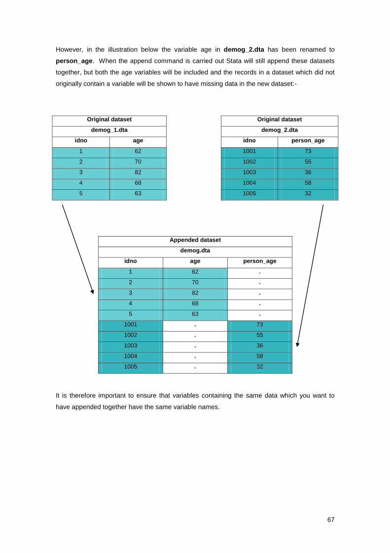
67
However, in the illustration below the variable age in demog_2.dta has been renamed to
person_age. When the append command is carried out Stata will still append these datasets
together, but both the age variables will be included and the records in a dataset which did not
originally contain a variable will be shown to have missing data in the new dataset:-
Original dataset
Original dataset
demog_1.dta demog_2.dta
idno age idno person_age
1 62 1001 73
2 70 1002 55
3 82 1003 36
4 68 1004 58
5 63 1005 32
Appended dataset
demog.dta
idno age person_age
1 62 .
2 70 .
3 82 .
4 68 .
5 63 .
1001 . 73
1002 . 55
1003 . 36
1004 . 58
1005 . 32
It is therefore important to ensure that variables containing the same data which you want to
have appended together have the same variable names.

68
To append datasets using Stata 12, first ensure that you have a dataset open onto which you
can append other datasets (this is referred to as your “master” dataset):-
use [filename]
Then use the following syntax to append the other datasets (termed “using” datasets) onto your
master dataset:-
append using [filename] [filename], [options]
So to append demog_2 and demog_3 onto demog_1.dta, the Stata 12 syntax would be:-
use demog_1
appending using demog_2 demog_3
save demog, replace
If the variables have the same name but have different types (for example if the age variable in
demog_1.dta is numeric but the age variable in demog_2.dta is string), Stata 12 will give an
error message. In these situations it is best to change the data types of some variables so that
they are all the same and the append can go ahead without error. You can use the force option
to append string or numeric variables together without error, although an error message will be
generated, and the using dataset(s) will contain missing data.
A useful option is generate (variable name), which gives a numeric value relating to the source
of the observations. Observations from the master dataset will be given the value 0, and those
from each subsequent using datasets will be given the value 1, 2, etc.
For more help on append syntax, type help append into the Stata command window.
Exercise 4 : Appending datasets
Append together demog_1, demog_2 and demog_3 and save this as a single recordset called
demog.
Check how many observations arein demog.dta (there should be 1624) and how much memory
is used.
Close the dataset.
Remember to include comments to keep a record of your work.

69
3.7 Naming variables, labelling variables and labelling values
In Practical 2 we saw how to label values in EpiData. However, it is common to come across
datasets where this has not been done, and it is useful to know how to label variables and
values in Stata.
It is important to understand the difference between labelling variable names and labelling
variable values.
3.7.1 Variable names
A variable name in Stata can be up to 32 characters long, must start with a letter and cannot
have any spaces. When analysing your data you will find that you repeatedly type your variable
names into the command window, and so it is good practice to keep the variable names as brief
as possible.
Should you wish to rename a variable, use the following syntax:-
rename existingname newname
So to rename the variable person_age to age, type:-
rename person_age age
3.7.2 Variable labels
In addition to its name, each variable has an 80-character variable label that is initially blank. It
is important to get into the practice of attaching labels to variables in order to provide more
detailed descriptions of the variables. This can be achieved with the command:-
label variable [varname] “information on variable”
For example, in the demog dataset you can give the variable idno a label to make it clear what
the variable is for:-
label variable idno “identification number”
Variable labels will be used in any output instead of the variable name if space allows.
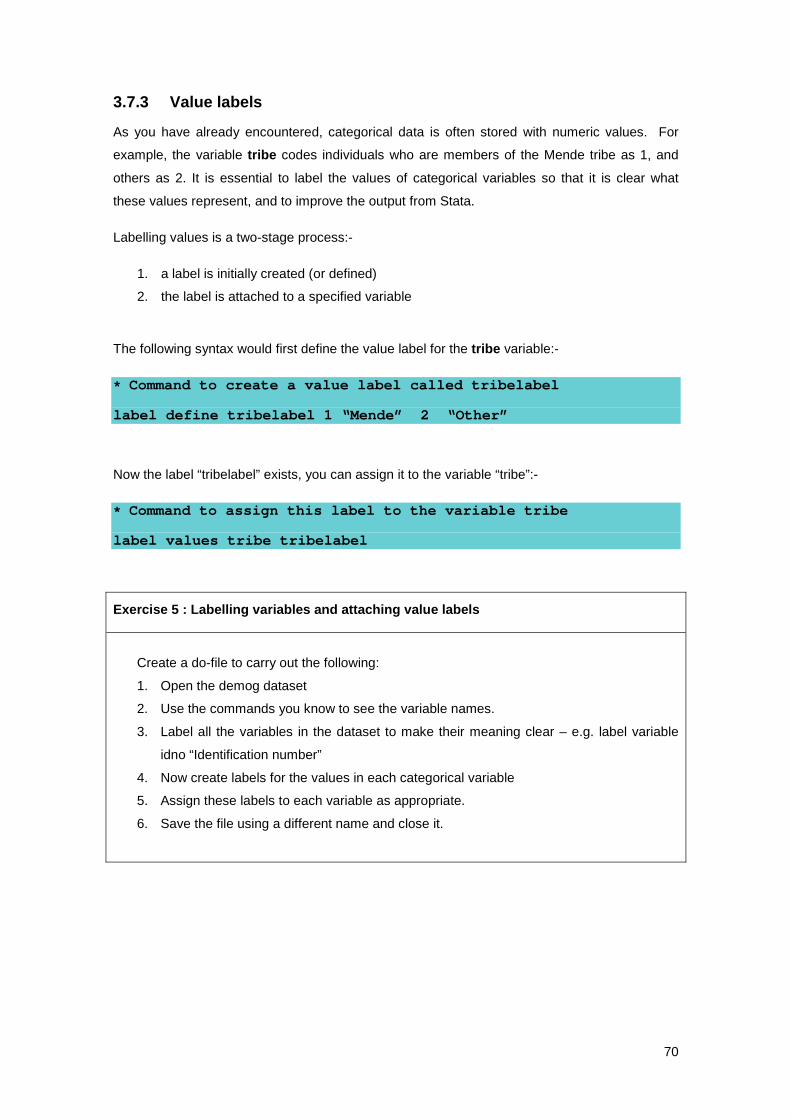
70
3.7.3 Value labels
As you have already encountered, categorical data is often stored with numeric values. For
example, the variable tribe codes individuals who are members of the Mende tribe as 1, and
others as 2. It is essential to label the values of categorical variables so that it is clear what
these values represent, and to improve the output from Stata.
Labelling values is a two-stage process:-
1. a label is initially created (or defined)
2. the label is attached to a specified variable
The following syntax would first define the value label for the tribe variable:-
* Command to create a value label called tribelabel
label define tribelabel 1 “Mende” 2 “Other”
Now the label “tribelabel” exists, you can assign it to the variable “tribe”:-
* Command to assign this label to the variable tribe
label values tribe tribelabel
Exercise 5 : Labelling variables and attaching value labels
Create a do-file to carry out the following:
1. Open the demog dataset
2. Use the commands you know to see the variable names.
3. Label all the variables in the dataset to make their meaning clear – e.g. label variable
idno “Identification number”
4. Now create labels for the values in each categorical variable
5. Assign these labels to each variable as appropriate.
6. Save the file using a different name and close it.

71
3.8 Describing data – list, tab, if, sort, by, means
list: If you simply type list, this will list all variables for all the observations. This is not
usually helpful because it contains too much information. To see all variables for a select
number of observations, type list in 1/10. This will list all variables in the first ten records
means: This gives the arithmetic, geometric and harmonic means. You can also obtain the
arithmetic mean with the summarize command. Simply type means and the variable name.
tabulate: The tab command gives frequencies (counts), and is most useful with
categorical variables. There are two ways to get one-way frequencies of variables:
For a single variable:
tab sex
For a list of variables displayed individually:
tab age-occ
To cross-tabulate two variables:
tab sex occ
You are likely to want percentages, in which case you must specify whether you want these calculated by row:-
tab sex occ, row
or by column:-
tab sex occ, col
To include observations where data are missing (often very important!), use:-
tab sex occ, missing
if: This is used to restrict analyses to a subset. For example, the command
tab occ if sex==1
will give the occupations of men in the population. Note that when you use the ‘if’ command you
must insert == .
sort: The sort command puts the observations in memory in ascending order of the
values of one or more variables. The gsort command enables you to sort in descending
order by placing a minus sign in front of the variable name e.g. gsort –idno will sort the
idno variable in descending order.
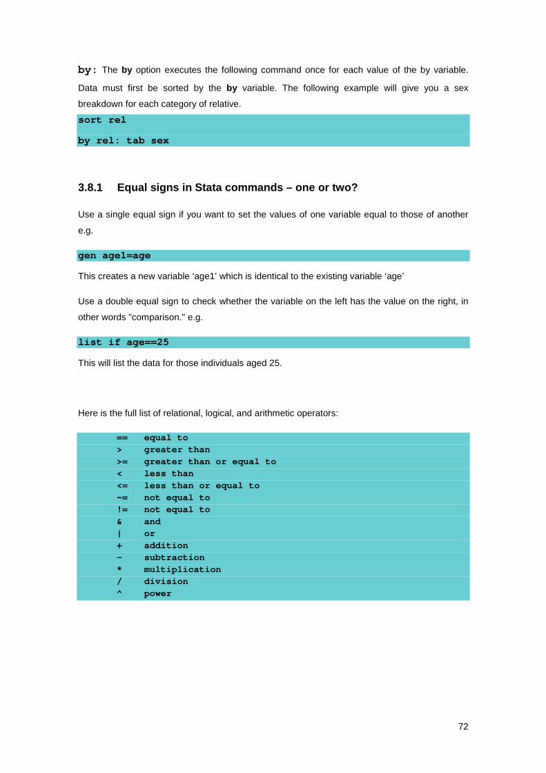
72
by: The by option executes the following command once for each value of the by variable.
Data must first be sorted by the by variable. The following example will give you a sex
breakdown for each category of relative.
sort rel
by rel: tab sex
3.8.1 Equal signs in Stata commands – one or two?
Use a single equal sign if you want to set the values of one variable equal to those of another
e.g.
gen age1=age
This creates a new variable ‘age1’ which is identical to the existing variable ‘age’
Use a double equal sign to check whether the variable on the left has the value on the right, in
other words "comparison." e.g.
list if age==25
This will list the data for those individuals aged 25.
Here is the full list of relational, logical, and arithmetic operators:
== equal to > greater than >= greater than or equal to < less than <= less than or equal to ~= not equal to != not equal to & and | or + addition - subtraction * multiplication / division ^ power
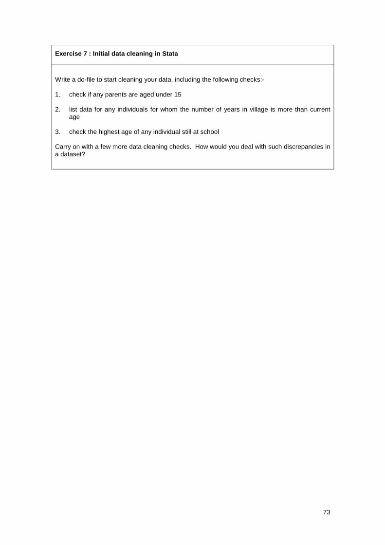
73
Exercise 7 : Initial data cleaning in Stata
Write a do-file to start cleaning your data, including the following checks:- 1. check if any parents are aged under 15 2. list data for any individuals for whom the number of years in village is more than current
age 3. check the highest age of any individual still at school Carry on with a few more data cleaning checks. How would you deal with such discrepancies in a dataset?

74
3.9 Creating and transforming variables: gen, replace, recode.
3.9.1 Recategorising data
In almost any analysis, you will want to recategorise data, or create new variables.
In Stata you can create new variables with generate and you can modify the values of an
existing variable with replace and with recode.
We often want to group values (e.g. age, BMI, haemoglobin count) and we have to decide on
appropriate cutpoints. There are two basic ways of doing this.
i) There may be a biological or physical rationale for choosing cutpoints e.g. there are
standard categories of body mass index (BMI) which correspond to underweight,
normal, overweight and obese.
ii) If there is no a priori reason to choose certain cutpoints, the preferable method is to
choose cutpoints that have roughly an equal number of observations in each group.
This tends to give the best power to detect associations in a dataset.
In either case, it is essential, that you do not make changes to the original variable because you
will lose the original data. Always make a copy of the variable you want to change.
Example: Changing occupation categories in the demog dataset
Supposing that we want to re-categorize occupation in the demog dataset to two broad
categories: Paid employment = 1 and unpaid employment = 2
To do this, first we create a new variable occup_gp identical to the variable occup
gen occ_gp=occ
Then we use the replace command to change categories as appropriate:
replace occ_gp=1 if (occ>=3 & occ<=6) | occ==8
replace occ_gp=2 if occ==1 | occ==2 | occ==7
What do you suggest we do with category 9 of occupation?
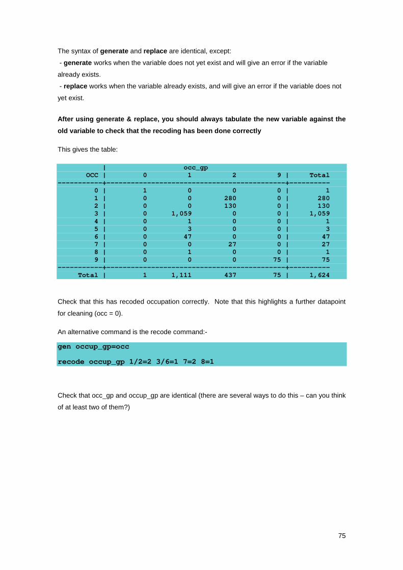
75
The syntax of generate and replace are identical, except:
- generate works when the variable does not yet exist and will give an error if the variable
already exists.
- replace works when the variable already exists, and will give an error if the variable does not
yet exist.
After using generate & replace, you should always tabulate the new variable against the
old variable to check that the recoding has been done correctly
This gives the table:
| occ_gp OCC | 0 1 2 9 | Total -----------+--------------------------------------------+---------- 0 | 1 0 0 0 | 1 1 | 0 0 280 0 | 280 2 | 0 0 130 0 | 130 3 | 0 1,059 0 0 | 1,059 4 | 0 1 0 0 | 1 5 | 0 3 0 0 | 3 6 | 0 47 0 0 | 47 7 | 0 0 27 0 | 27 8 | 0 1 0 0 | 1 9 | 0 0 0 75 | 75 -----------+--------------------------------------------+---------- Total | 1 1,111 437 75 | 1,624
Check that this has recoded occupation correctly. Note that this highlights a further datapoint
for cleaning (occ = 0).
An alternative command is the recode command:-
gen occup_gp=occ
recode occup_gp 1/2=2 3/6=1 7=2 8=1
Check that occ_gp and occup_gp are identical (there are several ways to do this – can you think
of at least two of them?)

76
3.10 The egen command In practical 3 you generated new variables using the ‘gen’ command to recode continuous
variables into groups. Suppose we want to create 10 year age categories.
We could create a new variable, recode and label the data as follows:
gen agegp=age
recode agegp min/9=1 10/19=2 20/29=3 30/39=4 40/49=5 50/59=6 60/max=7
label define agegp 1 “<10” 2 “10-19” 3 “20-29” 4 “30-39” 5 “40-49” 6 “50-59” 7 “>60”
label values agegp agegp
tab agegp
Alternatively, we can use a new command egen. egen stands for extended generate and is an
extremely powerful command that has many options for creating new variables.
The syntax of any egen command is
egen newvarname= option (varname), additional instructions
Options include:
cut groups values into pre-defined categories count number of non-missing values diff compares variables, 1 if different, 0 otherwise fill fill with a pattern group creates a group id from a list of variables iqr interquartile range ma moving average max maximum value mean mean median median min Minimum value pctile percentile rank rank rmean mean across variables sd Standard deviation std Standard scores sum sums
Here, we are using the cut option.

77
egen agegp = cut(age), at(0,10(10)60,100) label
This means:-
create a variable agegp which is cut at 0, at 10 years then at every 10 years until 60, then at
100 years. The ‘label’ option automatically labels the variable.
Alternatively, we could ask cut() to choose the cutpoints to form agegroups with approximately
the same number per group. Below we request the creation of 5 (roughly) equally sized groups.
egen agegp5 = cut(age), group(5) label
Use the tab command to see which cutpoints Stata has chosen. Which grouping of age would
you prefer?
The command
egen mean_age=mean(age)
creates a new variable mean_age which contains the mean age in the sample.
Exercise 8 : egen command
Type the command below and interpret:
egen mean_age=mean(age), by(sex)
3.10.1 What’s the difference between gen and egen?
The generate command has functions to create unique values on each observation. The egen
command has a different set of functions. Some of its functions put unique values on each
observation, while others put summary statistics across all observations (or groups) on each
observation. For example, suppose we had a file containing the age of each person in a
household. In this file, each person is an observation, and there are multiple households of
people in the file. The following generate command would calculate the natural log of the age of
each person and add that value to each person's record:
gen lage=log(age)

78
In contrast, the following egen command would calculate the median age of all members of
each household, and it would add that value to each household member's record:
sort hhno
by hhno: egen medage=median(age)
3.11 Exercise
One of the principal outcomes in this study is the presence or absence of microfilariae in skin
samples at survey round 5. In the data file micro.dta, the variables MFRIC and MFLIC contain
the numbers of microfilariae observed in the right and left skin samples (see box below)
MICRO.REC IDNO Subject ID number
microfilariae counts SR Survey round 1 ... 5
MFRIC MF count (right) Positive integers 999
MFLIC MF count (left) Positive integers 999
SSRIC Skin diameter (right) Positive real numbers
SSLIC Skin diameter (left) Positive real numbers
(The variables SSRIC and SSLIC record the diameters of the right and left skin samples. We
aren’t going to use these variables in this course.)
We should undertake three tasks with this file before it is ready for data analysis.
These are:
a) Recode missing value codes to missing (blank) values.
b) Create a variable containing the numbers of microfilariae observed in both skin snips.
c) Create a variable that indicates the presence of microfilariae in either skin snip.

79
Exercise 9 : Creating new variables to answer the research question Instruction
Hint
a. Open the dataset micro.dta. Have an initial look at the data.
Use summarize and codebook
b. The missing value code for mfric and mflic is 999. Use the recode command to replace these values to be coded as missing in Stata (“.”)
Use recode then tab to check recoding
c. Create a variable (mftot) that contains the total number of microfilariae observed in both skin snips. Check your new variable has been created correctly for the first 20 records
Use gen, then use list.
d. Now create a variable (mf), based on mftot, which is a binary variable showing presence/absence of microfilaria. What value of mf do you give to people with missing values of mf counts?
Code 1 = with microfilaria, 0 = without.
e. For some analyses, we will want a categorical variable for mf count. Create a variable mfcat which has the following values: Zero for mf = 0 1 for mf counts between 1 and 49 2 for mf counts greater or equal to 50
Use gen or replace or an egen command
f. Save your edited dataset as micro1.dta
Use this data set to answer the following: How many individuals had microfilariae present? What was the average number of mf present among those who tested positive? (Is it better to use the arithmetic or geometric mean?)
Use the command means variable
80
Data Management using EpiData and Stata
Practical 4 : Data Management using Stata 12
II : Essentials
Objectives of this session
In this session we cover some more advanced data management, including changing variable
types and changing the structure of datasets using commands such as collapse, reshape and
merge. There is then a more open-ended exercise which will give you the opportunity to
practice your data management skills.
By the end of this session you should be able to:
• Convert between numeric & string variables
• Collapse datasets
• Reshape data from long to wide format
• Merge two datasets together
4.1 Types of variable – string and numeric
4.1.1 Converting string variables to numeric (destring, encode)
Stata can store data in string variables, which may contain letters and numbers, or in numeric
variables which can contain only numbers. In terms of analysis, there is little that you can do
with numeric data which has been stored in a string variable – you cannot calculate sums or
means, or carry out a t-test, etc. It is therefore important to store your continuous numeric data
(age, blood pressure, cholesterol, etc) in numeric variables. However, you may receive a file
which has numeric data stored in string variables. The destring command in Stata is useful for
converting a string variable to a numeric one.
For this exercise we will use a different dataset – hsbs – which is a small sample of high school
data with all of the data stored in string variables. Open the hsbs dataset and inspect the data
using the describe command. As you see from the describe command below, the variables are
all stored as string variables (e.g. science is str2, a string of length 2).
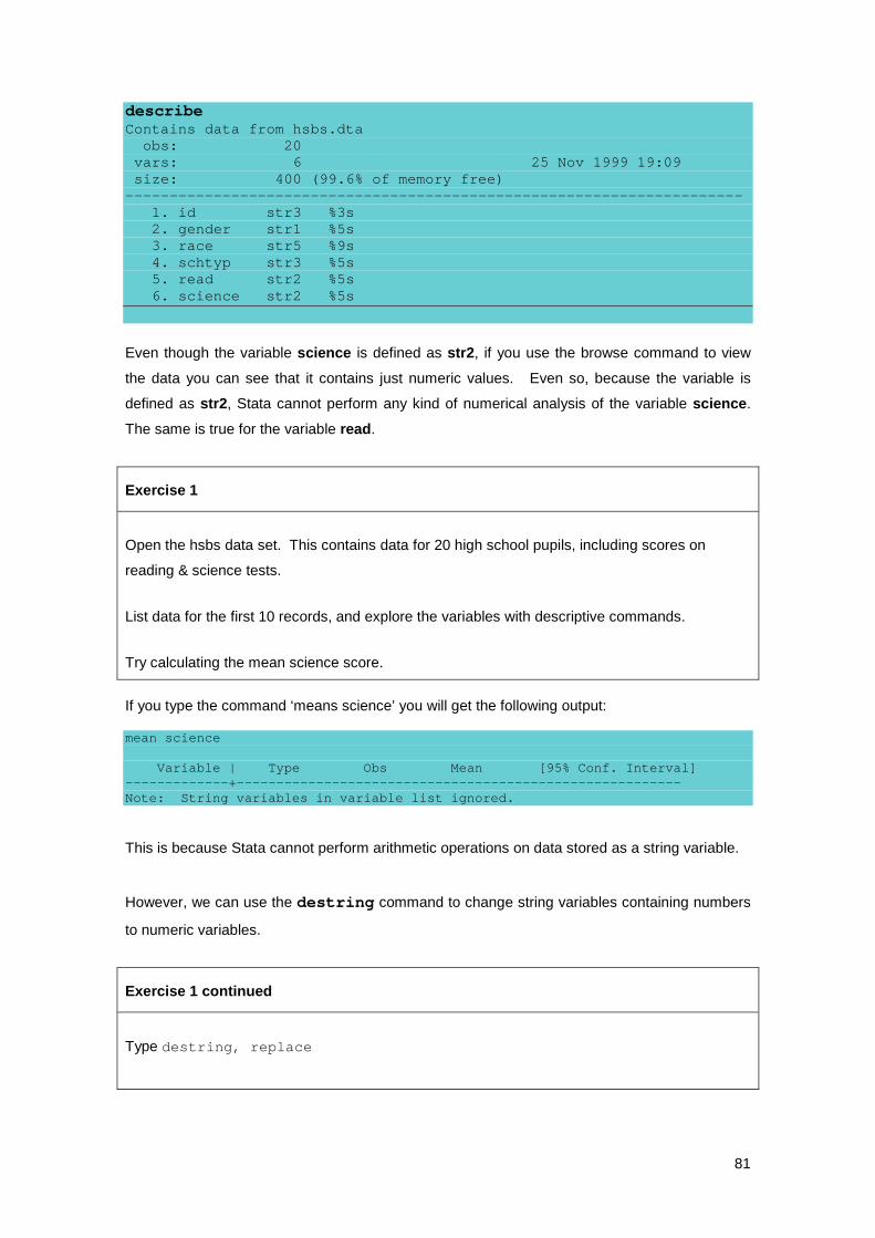
81
describe Contains data from hsbs.dta obs: 20 vars: 6 25 Nov 1999 19:09 size: 400 (99.6% of memory free) ---------------------------------------------------------------------- 1. id str3 %3s 2. gender str1 %5s 3. race str5 %9s 4. schtyp str3 %5s 5. read str2 %5s 6. science str2 %5s
Even though the variable science is defined as str2, if you use the browse command to view
the data you can see that it contains just numeric values. Even so, because the variable is
defined as str2, Stata cannot perform any kind of numerical analysis of the variable science.
The same is true for the variable read.
Exercise 1
Open the hsbs data set. This contains data for 20 high school pupils, including scores on
reading & science tests.
List data for the first 10 records, and explore the variables with descriptive commands.
Try calculating the mean science score.
If you type the command ‘means science’ you will get the following output: mean science Variable | Type Obs Mean [95% Conf. Interval] -------------+-------------------------------------------------------- Note: String variables in variable list ignored. This is because Stata cannot perform arithmetic operations on data stored as a string variable.
However, we can use the destring command to change string variables containing numbers
to numeric variables.
Exercise 1 continued
Type destring, replace
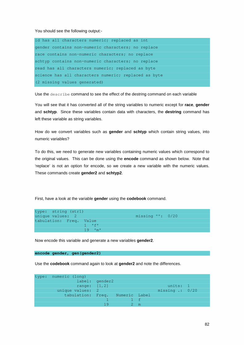
82
You should see the following output:- id has all characters numeric; replaced as int
gender contains non-numeric characters; no replace
race contains non-numeric characters; no replace
schtyp contains non-numeric characters; no replace
read has all characters numeric; replaced as byte
science has all characters numeric; replaced as byte
(2 missing values generated)
Use the describe command to see the effect of the destring command on each variable
You will see that it has converted all of the string variables to numeric except for race, gender and schtyp. Since these variables contain data with characters, the destring command has
left these variable as string variables.
How do we convert variables such as gender and schtyp which contain string values, into
numeric variables?
To do this, we need to generate new variables containing numeric values which correspond to
the original values. This can be done using the encode command as shown below. Note that
‘replace’ is not an option for encode, so we create a new variable with the numeric values.
These commands create gender2 and schtyp2.
First, have a look at the variable gender using the codebook command.
type: string (str1) unique values: 2 missing "": 0/20 tabulation: Freq. Value 1 "f" 19 "m"
Now encode this variable and generate a new variables gender2.
encode gender, gen(gender2)
Use the codebook command again to look at gender2 and note the differences.
type: numeric (long) label: gender2 range: [1,2] units: 1 unique values: 2 missing .: 0/20 tabulation: Freq. Numeric Label 1 1 f 19 2 m
83
Exercise 2
Encode the variable schtype and generate a new variable schtype2
Now look at the variable race. Was this converted during the destring command? What is the
value for ‘missing’ for this variable?
If you tabulate race, you will see that there is one missing observation, which has been coded X.
So race remained as a character variable because the destring command saw the X in the data
and did not attempt to convert it because it had non-numeric values.
Below we can convert it to numeric by including the ignore (X) option that tells destring to
convert the variable to numeric and when it encounters X to convert that to a missing value.
destring race, replace ignore(X)
race: characters X removed; replaced as byte
(1 missing value generated)
As you have seen, we can use destring to convert string variables that contain numbers into
numeric variables, and it can handle situations where some values are stored as a character
(like the X we saw with race). If you have a character variable that is stored as all characters,
you can use encode to convert the character variable to numeric and it will create value labels
that have the values that were stored with the character variable.
4.1.2 Converting numeric values to string (decode) Conversely, one may wish to convert a numeric variable to a character. This is possible if a
label values have been assigned to the numeric variable. The new character variable then
takes the values of the label.
For example, we could turn the gender variable back into a string variable using the label values
1=f, 2=m
The command:-
decode gender2, gen(gender3)
will create a new variable gender3 with the values f’ and ‘m’ instead of 1 and 2. This is identical
to the original variable gender.

84
4.2 Collapsing datasets
Often a dataset will contain records relating to individuals who may share a common
characteristic, such as living in the same household or village. It can be useful to examine the
data in terms of such a characteristic, such as the number of individuals in a village or the mean
age in a household. This can be achieved using the collapse command.
The collapse command can be more useful than simple tabulations because it physically
restructures the dataset into a form which can then exported into another application (such as
an Access or Word table), or displayed as a Stata graph.
However, because the collapse command physically changes the structure of your data, it is
vital that you save any collapsed datasets with a different name to your original dataset –
otherwise you can permanently lose important individual-level data!
The effect of the collapse command can be seen in the example below. The first table shows a
person ID, household ID and ages of ten individuals live in four households. In the second table
the data have been collapsed to one record per household, with new variables giving the
number of individuals and mean age in each household.
person_id household age 1001 1 73 1002 1 37 1003 1 15 1004 1 36 1005 2 30 1006 2 36 1007 3 40 1008 4 12 1009 4 24 1010 4 28
Table 1 : “raw” data showing a record for each individual
Household number of individuals mean age 1 4 40.25 2 2 33 3 1 40 4 3 21.33
Table 2 : “collapsed” data, showing a record for each household with calculated variables
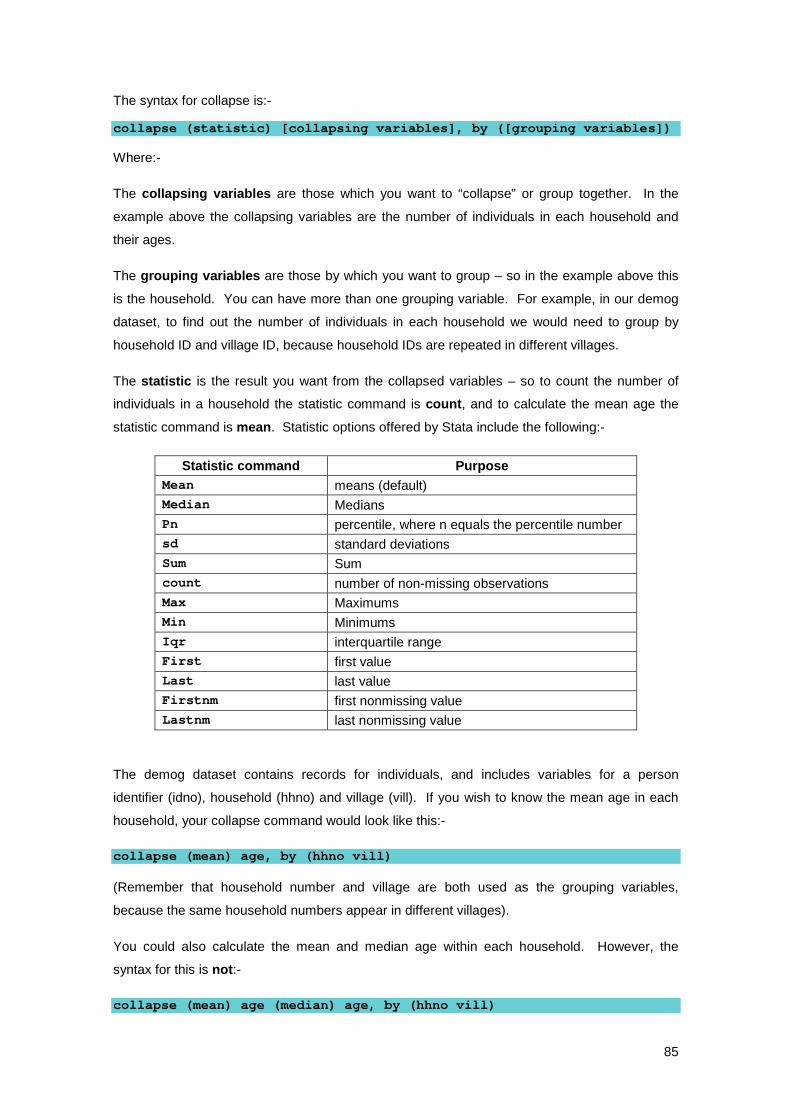
85
The syntax for collapse is:-
collapse (statistic) [collapsing variables], by ([grouping variables])
Where:-
The collapsing variables are those which you want to “collapse” or group together. In the
example above the collapsing variables are the number of individuals in each household and
their ages.
The grouping variables are those by which you want to group – so in the example above this
is the household. You can have more than one grouping variable. For example, in our demog
dataset, to find out the number of individuals in each household we would need to group by
household ID and village ID, because household IDs are repeated in different villages.
The statistic is the result you want from the collapsed variables – so to count the number of
individuals in a household the statistic command is count, and to calculate the mean age the
statistic command is mean. Statistic options offered by Stata include the following:-
Statistic command Purpose Mean means (default) Median Medians Pn percentile, where n equals the percentile number sd standard deviations Sum Sum count number of non-missing observations Max Maximums Min Minimums Iqr interquartile range First first value Last last value Firstnm first nonmissing value Lastnm last nonmissing value
The demog dataset contains records for individuals, and includes variables for a person
identifier (idno), household (hhno) and village (vill). If you wish to know the mean age in each
household, your collapse command would look like this:-
collapse (mean) age, by (hhno vill) (Remember that household number and village are both used as the grouping variables,
because the same household numbers appear in different villages).
You could also calculate the mean and median age within each household. However, the
syntax for this is not:-
collapse (mean) age (median) age, by (hhno vill)
86
This is because the age variable appears twice, and Stata cannot create two variable with the
same name. The solution to this is to give the collapsed variables new names (this is generally
good practice because it makes the resulting collapsed dataset easier to understand). So the
syntax above could, for example, read:-
collapse (mean) meanage = age (median) medage = age, by (hhno vill)
Note that, as the collapse command creates a new dataset, the original value labels will be lost.
However, the original label lists will be retained, so you simply need to re-apply the label values
to the variables using the “label values” command.
Exercise 3 – using the collapse command
Open the demog file again and collapse the dataset so you have a line giving the number of
people within each household, within each village. Sort the resulting dataset by village and
household, and then browse the results. How many people live in household 16 in village 5?
How many households are there in village 4?
4.3 Reshaping data
Last week we appended the three demog_ files together into one long demog file containing
data on all individuals. Now we are going to combine this baseline demographic data with
laboratory data and treatment codes.
One of the research questions in this trial was whether the drug ivermectin was associated with
a lower prevalence of microfilaria at survey round 5. We will see how to create an appropriate
dataset in order to answer this question.
At the end of this session, you will have a file called oncho_all.dta which contains all the
necessary information for each individual. This file can then be used for data analysis.
Exercise 4
Open the file micro1 and explore this data using the describe, summarise and codebook
commands. How many individuals were seen in survey round 1? How many in survey round
5? Use the list, edit, browse or tab command to work out how the data is organised.
For data analysis, we want to have just one line of data for each individual. This means that all
the data from each individual should be stored on the same line of data so that, for example, a
comparison of the density of microfilariae between the two survey rounds can be made.

87
The micro1 dataset contains one line per survey round for each individual. To get one line per
individual, we need to use the reshape command in Stata. Reshape is a very powerful
command which changes the structure of a file.
The tables below show the data for the first ten patients in the micro1 dataset in both long and
wide format. The examples use just the idno, sr and mfric variables.
In table 1, the data are shown in long format; the mfric values recorded at each survey round
are shown on a separate line, and so in these cases there are two records for each patient.
You will see the data in this format if you open the micro1 dataset and type browse into the
command window.
idno sr mfric 1 1 47 1 5 1 2 1 56 2 5 36 3 1 0 3 5 0 4 1 14 4 5 9 5 1 11 5 5 1
Table 2 below shows the same data in wide format. Here there is one line of data per
individual, and the microfilaria count at survey rounds one and five are shown in two variables.
The actual values in the original survey round variable (1 or 5) have been used to create the
variable names mfric1 and mfric5.
idno mfric1 mfric5 1 47 1 2 56 36 3 0 0 4 14 9 5 11 1
Table 2 : Data in wide format
88
The syntax for reshaping from long format to wide format is:-
reshape wide var1…var[n], i(var2) j(var3)
Where:-
var1…var[n] are the variables currently in long format which are to be converted to wide
format.
i(var2) is the variable which uniquely identifies variables, such as the person ID number
(idno). This is called the logical observation.
j(var3) is the variable which uniquely identifies each separate record within the group of
records for that individual. In this case it is the sr variable, which uniquely identifies the survey
round for each individual as either 1 or 5. This is called the sub-observation. Stata uses the
value of this variable to create new variable names in the wide format. In this case the values in
the sr variable (1 or 5) are used to create the new variables mfric1 and mfric5. The original sr
variable is dropped from the dataset in the process of reshaping the data because it is no longer
required.
All of the variable names in a dataset need to be included in the reshape command in order for
it to function correctly. For this reason it can be useful to reduce a dataset so that it only
contains the variables that you really need in the reshaped dataset.
Exercise 5 – using the reshape command to obtain one line of data per individual
Use the reshape command to change the dataset micro1 from long to wide format so you
have one line per individual, and create variables for mf counts at each survey round. Include all
of the variables in the current dataset.
List the data for the first few observations to see how the variables and structure of the dataset
have changed.
Save this new dataset as microwide
Use help reshape for further help on using this command

89
Listing data for the first two individuals we see:
list in 1/2 Observation 1 idno 1 mfric1 47 ssric1 2.2 mflic1 15 sslic1 2 mftot1 62 mf1 1 mfric5 1 ssric5 2.5 mflic5 0 sslic5 1.9 mftot5 1 mf5 1 Observation 2 idno 2 mfric1 56 ssric1 1.9 mflic1 10 sslic1 2.1 mftot1 66 mf1 1 mfric5 36 ssric5 1.5 mflic5 19 sslic5 1.8 mftot5 55 mf5 1
Exercise 5 continued
Open the dataset named blood. Change the dataset blood from long to wide format so you have one line per individual, and
create variables for test outcomes at each survey round.
List the data for the first few observations to see how the variables and structure of the dataset
have changed.
Save this dataset as bloodwide
4.4 Merging files
Merge is an important command in Stata. Any time that you want to add information from one
dataset to another, matching on a case-by-case basis, you will need to merge. The merge
command joins two files together next to each other in a “parallel” fashion. This differs from the
append command covered in the last session, in which files with the same structure are added
“end-to-end”.

90
Stata merges files by matching records from each file according to key variable(s) which you
define. For example:-
Original dataset (master)
Original dataset (using) idno age idno sex
1 62 1 M 2 70 2 F 3 82 3 F 4 68 5 F 5 63 6 M 6 73 9 F 7 55 10 M 8 36 11 M 9 58 12 F 10 32 13 M
Merged dataset idno age sex _merge
1 62 M 3 2 70 F 3 3 82 F 3 4 68 . 1 5 63 F 3 6 73 M 3 7 55 . 1 8 36 . 1 9 58 F 3 10 32 M 3 11 . M 2 12 . F 2 13 . M 2
The “master” dataset describes the dataset which is opened first, whilst the “using” dataset
describes the second dataset which is merged into the master dataset.
You can see in the example above that, whilst both original datasets contain 10 records, the
“master” dataset does not contain records for patients 11, 12, and 13, whilst the “using” dataset
does not contain records for patients 4, 7 and 8. The resulting merged dataset contains records
for all 13 patients, but there are missing data for where records were absent in either the master
or using datasets.

91
When carrying out a merge, Stata will automatically generate a new variable called _merge.
This will contain a value of either 1, 2 or 3 which indicates which records were merged:-
_merge==1 if a record is present in the master data but has no match in the using data.
_merge==2 if a record is present in the using data but has no match in the master data.
_merge==3 if a record is present in both the master and using datasets.
Stata 12 will automatically tabulate the merge variable for you once the merge command has
been run, for example:-
Result # of obs. ----------------------------------------- not matched 80 from master 0 (_merge==1) from using 80 (_merge==2) matched 2,855 (_merge==3) -----------------------------------------
For a merge to take place there must be at least one variable of the same name and type which
is common to both the Master and Using datasets. In the example above this variable is the
unique patient identifier (idno). It is possible to merge on more than one key variable – for
example, you may have a dataset composed of multiple follow-up visits for each patient, in
which each patient would have a unique id, and the set of visits for each patient would also
have a unique id, as in the example below:-
Original dataset (master)
Original dataset (using) idno visitno temp ˚C idno visitno cholesterol
1 1 37.6 1 1 4.9 1 2 36.2 1 2 5.2 2 1 36.1 2 1 5.8 2 2 35.4 2 2 6.0 2 3 34.9 2 3 5.3
In such a case it is important to specify both your patient identifier and your visit identifier in the
merge command for the records to be joined correctly.
Note that, in the example above, having repeated idno and visitno in each dataset does not
constitute duplicate records because it is the combination of the idno and visitno variables
which uniquely identifies each record.
A new feature in Stata 11 and 12 is that you need to specify the type of merge that you are
carrying out as part of the syntax. Merge types can take the following forms:-

92
1:1 A one-to-one merge. In both the master and the using datasets the key variable(s)
uniquely identify each record, with no duplicates within each dataset.
1:m A one-to-many merge. The key variable(s) are not duplicated in the master recordset,
but are duplicated in the using dataset. Stata will still merge using the key variable(s)
but in this case, where a merge takes place, the record in the master dataset will
become duplicated.
m:1 A many-to-one merge. The key variable(s) are duplicated in the master dataset but are
unique in the using dataset. In this instance the merge will still take place on the key
variable(s) but the data in the using dataset will become duplicated where a merge
takes place.
m:m A many-to-many merge. The key variable(s) are duplicated within both datasets, and
Stata will create duplicates in both records where a merge takes place.
The syntax to create a 1:1 merge between a master and using dataset using idno as the key
variable is as follows:-
use [masterdataset]
merge 1:1 idno using [usingdataset]
The syntax for a 1:1 merge using more than one key variable, such as idno and visitno, would
be:-
use [masterdataset]
merge 1:1 idno visitno using [usingdataset]
Note that in Stata 11 and 12 the recordsets do not have to be sorted on the key variable(s) first.
In the following exercise we will merge the following three files:
Demog.dta - baseline demographic data
Microwide.dta – lab data containing MF prevalence in surveys 1 and 5
Tmtcodes.dta – drug treatment data (ivermectin or placebo)
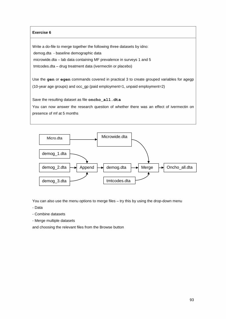
93
Exercise 6
Write a do-file to merge together the following three datasets by idno:
demog.dta - baseline demographic data
microwide.dta – lab data containing MF prevalence in surveys 1 and 5
tmtcodes.dta – drug treatment data (ivermectin or placebo)
Use the gen or egen commands covered in practical 3 to create grouped variables for agegp
(10-year age groups) and occ_gp (paid employment=1, unpaid employment=2)
Save the resulting dataset as file oncho_all.dta
You can now answer the research question of whether there was an effect of ivermectin on
presence of mf at 5 months
You can also use the menu options to merge files – try this by using the drop-down menu
- Data
- Combine datasets
- Merge multiple datasets
and choosing the relevant files from the Browse button
demog_1.dta
demog_2.dta
demog_3.dta
Append
tmtcodes.dta
Merge Oncho_all.dta demog.dta
Micro.dta Microwide.dta
Sr = 1 // Sr = 5
94
Data Management using EpiData and Stata
Practical 5 : Data Management using Stata 12
III : Advanced
Objectives of this session
In this final session, we look at dates, simple programming, and subgroups. There is then an
open-ended exercise which will give you the opportunity to practice your data management
skills.
By the end of this session you should be able to:-
• Format dates in Stata
• Be aware of simple Stata programming using the foreach loop
• Identify duplicate observations
• Use system variables to work with sub-groups.
5.1 Dates The key principle when using dates in Stata is that dates are stored as the number of days since 1st Jan 1960. If a date falls before this reference date then the date is stored as a minus
number. So 1st January 1960 is stored as 0, 2nd January 1960 is stored as 1, and 31st
December 1959 is stored as -1, and so on.
To see how a date is stored in Stata, use the display command and the mdy function. The
examples below give examples of this for three dates, with the resulting output shown directly
beneath the display command.
display mdy(01,01,1960) 0 display mdy(12,31,1959) -1 display mdy(10,22,2010) 18557

95
Having dates stored as single numbers means that the duration between two dates can easily
be calculated as the difference between the two numbers.
The date can be displayed as a number or it can be formatted to be displayed in a useful way.
For example a date can be displayed as 6 Dec 2001 even though it is stored as 15315. To
format a date use the format command with a variable name and the suffix %td, for example:-
format dob %td
If we want to calculate the dates of birth of the respondents in the demog dataset, there are
therefore two stages to the process:-
a. calculate how many days before or after 1st January 1960 the person was born
b. format the number of days into a date.
Exercise 1 – calculating the date of birth
Open the demog dataset, list the variables date and age.
We want to calculated date of birth. We know the date of the interview. This is stored as a
number but displayed as a date. Now we want to subtract the age of the respondent in days
from the date of the interview. We can do this by subtracting age (in days – so age*365.25)
from current date.
Generate the variable dob that lists date of birth as a number
Now list the three variables date, age and dob for the first 10 individuals.
Why are some values negative?

96
You can also format in units of a week, a month, a quarter or a half-year.
+---------------------------------------------------------------------+ | | | ----- Numerical value & interpretation ------ | | Format | Meaning | Value = -1 | Value = 0 | Value = 1 | |--------+------------+---------------+---------------+---------------| | %tc | clock | 31dec1959 | 01jan1960 | 01jan1960 | | | | 23:59:59.999 | 00:00:00.000 | 00:00:00.001 | | | | | | | | %td | days | 31dec1959 | 01jan1960 | 02jan1960 | | | | | | | | %tw | weeks | 1959w52 | 1960w1 | 1960w2 | | | | | | | | %tm | months | 1959m12 | 1960m1 | 1960m2 | | | | | | | | %tq | quarters | 1959q4 | 1960q1 | 1960q2 | | | | | | | | %th | half-years | 1959h2 | 1960h1 | 1960h2 | | | | | | | | %tg | generic | -1 | 0 | 1 | +---------------------------------------------------------------------+
Exercise 1 – continued
Format the values in the dob variable so they are displayed in a useful way.
What is the date of birth of the oldest and the youngest person of the people surveyed?
For further information on dates, use the help dates command. This facility is useful for
calculating other dates such as date of next treatment (e.g. in 45 days) or the date of expected
delivery.
97
5.2 Identifying duplicate observations
Detecting duplicate observations is an essential part of data management and analysis. In
Stata terms, duplicates are observations with identical values, either on all variables or on a
specified varlist (often ID number).
The basic command in Stata to detect duplicates is duplicates. Suppose we want to know
about duplicate ID numbers. The possible commands are:-
duplicates report id
- this shows how many unique and duplicate entries there are
duplicates list id
- this lists ID number for those observations with duplicate ID
duplicates drop id, force
- this drops all but one observation from each group of duplicates i.e. dropping the surplus
observations.
Do be sure, however, that you really want to drop duplicates. You may have duplicate identity
numbers because you have recorded information for one person relating to different events, or
at different time periods.
The force option is required when such a varlist is given as a reminder that information may be
lost by dropping observations, because the ‘duplicate’ observations may differ on other
variables which are not included in varlist.
You can also access these commands from the Data menu, by going to the option ‘Data
utilities’, and then ‘Manage duplicate observations’. This gives several
options, but a useful one is to list all duplicate observations. To do this, click on ‘List all
duplicates’ and enter idno in the variable box. If you try this for the demog dataset there
should be no duplicates.

98
Exercise 2 : Duplicate observations
Open the micro1 dataset and investigate duplicate idno values.. How many individuals have more than entry? Why are there so many duplicates in this dataset?
5.3 Shortcuts for repeating commands: using foreach loops We often need to run the same command for a large number of variables. For example, we
might want to change the value 9 to missing for 200 variables in a data file. We can type the
recode command 200 times, or we can type the foreach command once and let it create 200
copies of recode for us.
Recode can also rename a group of variables, saving us typing many rename commands. In
fact any command, or set of commands, that you need to repeat over a group of variables is a
likely candidate for one of these labour-saving commands.
For example, in analysing the Onchocerciasis data, you would probably want to summarise the
prevalence of mf at round 5 by each of the socio-demographic variables. You can do this by
using the tab command and apply it to all the socio-demographic variables by using the
foreach command.
First we must group the variables in which we are interested.
use oncho_all
order agegp sex tribe occup_gp
Next we have three lines of command. The first instructs Stata which variables we want
the tab command to apply to, the second is the command itself, the third instructs
Stata that the foreach command is closed.
99
The three lines look like this.
foreach var of varlist agegp-occup_gp {
tab `var' mf5
}
NOTE: The ` is usually the top left hand key of your keyboard (or may be to the left of the space
bar). The ' is the quote usually on the same key as @.
What is the foreach statement?
The foreach statement tells Stata that we want to cycle through the variables agegp to
occup_gp using the statements that are surrounded by the curly braces. The first time we
cycle through the statements, the value of var will be agegp and the second time the value of
var will be sex and so on until the final iteration where the value of var will be occup_gp.
Each statement within the loop (in this case, just the one tab statement) is evaluated and
executed. When we are inside the foreach loop, we can access the value of var by surrounding
it with the strange quotation marks like this `var' . The first time through the loop, `var' is
replaced with agegp, so the statement becomes
tab agegp mf5
This is repeated for sex and then tribe and then occup_gp.
So, this foreach loop is the equivalent of executing the four tab statements manually, but is
much easier and less error-prone. You can see that this will save a lot of time when you have
many variables, and more complex commands to be executed for each one.
Exercise 3 : Using the foreach loop
Use the foreach commands above to calculate the prevalence of mf at round 1 by
occupation, tribe and age in that order..

100
5.4 Working with sub-groups – the use of the Stata system variables _n and _N
Stata has two internal variables. These are always present but unseen.
_n is the record number and _N is the number of records. This may not sound very useful but
because these variables exist for any number of groups, as defined by sorting the data (“sort
groups”), they are very helpful when working within these sub-groups or clusters.
Supposing we have a file (such as hh_long.dta) which is a file of household members, in long
format, with a household id (hid) and a person number (pno) for each person in the household
(1, 2, 3, ...).
A common requirement when working with such structured data is the need to assign all
individuals with a group (household) a value derived from another individual in the group, or
from the group as a whole. For example, you may wish to give all family members the social
class of the household head.
The first step would be to sort by hid and pno:-
use hh_long, clear
sort hid pno
then records are grouped by hid and within household are in number order. The groups by
which the file is now structured (i.e. by household – sorted on hid) is called the sort group.
Within each sort group _n and _N exist as record number and total number in the group
respectively. You can turn these into variables.
by hid: gen littlen=_n
by hid: gen bign=_N
list hid pno littlen bign in 1/5

101
+--------------------------------+
| hid pno littlen bign |
|--------------------------------|
1.| 1000209 1 1 1 |
2.| 1000381 1 1 2 |
3.| 1000381 2 2 2 |
4.| 1000667 1 1 1 |
5.| 1001221 1 1 2 |
|--------------------------------|
So what use is this? In the panel above bign has effectively labelled each household member
with the total number in the household.
Exercise 4 : Using _n and _N
Open the hh_long dataset.
In this dataset we assume that the first respondent is the head of household. Your task is to find
out the proportion of heads of household who are men.
[Hint: the first respondent will have _n=1
Sort by household and individual identity number
Assign values for _n and _N
Assess what proportion of those with _n=1 are male]
102
In addition each record in a sort group can be accessed individually. Supposing we have
records sorted so that the head of household is always the first record of a household. To
identify the record of each head of household we have to use the square brackets [ ].
the age of the household head would be age[1]
the age of the third person listed would be age[3]
the age of the last person listed would be age[_N]
This is powerful because now we can create new variables that have a common value for
everyone within a household. Suppose we want a variable that assigns to everyone in a
household the value of the age of the household head.
by hid: gen agehh= age[1]
Note that you must use the
by groupname:
for this command to make sense.

103
5.5: Final data management exercise – this will give you some practice at using egen commands, _n, merging and reshaping data. You are now working as an advanced Stata user!
1. Use the hh_long dataset to answer the following:-
How many households are there?
[Hint: use the codebook command]
What is the maximum number of individuals per household
[Hint: use _n but don’t forget to sort by household id first]
2. Create a variable for each individual which is their household size.
[Hint: use egen with the (max) option]
3. Create a new variable which is the average age in each household. Also calculate the
overall mean age among adults and children (defined as <15) respectively).
4. Save your dataset as hh_long_1. Then create a new dataset called hh_siblings_long,
which contains only individuals identified as ‘natural children’ by variable relation. (We
will assume that natural children within the same household are siblings). How many
individuals are there in this new dataset? Check the maximum age.
5. Create a variable for birth interval between successive siblings with the commands
[Hint: first sort on hid and age, and then use the command
by hid: gen interval = age[_n+1] – age]
6. List the variables hid, relation, age and interval for the first 10 observations to check that
this has correctly calculated the age interval between children. Why is the variable
‘interval’ missing for so many observations?
7. Save this file as hh_siblings_long_1.
8. Now open the dataset hh_long_1 which contains data on all individuals, not just
siblings. Reshape this file to the wide format to obtain one line per household. Check
that the number of lines is the same as that obtained in question 1.
[Hint: the variables to include in the reshape wide line are those which differ for different
individuals within a household]
9. Merge this dataset with the file hh_sclass which contains the social class for each
household (one line per household). What is the distribution of social classes in this
sample.
Suppose we now want to create a subset of the data containing only spouses. We can
do this by reshaping the data to long to select individuals we want and then reshaping
back to wide. Once you get used to reshaping data, you will find it very useful as some
data manipulations lend themselves to long data and some to wide.
Continued…

104
10. Use the reshape long command to reshape the data back to a long dataset.
[Note: you will need to first drop the _merge variable. Also note that after reshaping,
the individuals within a household are identified by a newly created variable _j]
11. Create a subset of this dataset which contains only spouses
12. Finally, reshape the data to wide format, and calculate the age difference between
spouses. List households with any unusual age differences.
1
APPENDIX 1
Multicentre study of factors affecting the spread of HIV in African towns
Data Processing Manual
June 1997
2
CONTENTS
Topic Page Introduction 3 Filenames 4 Flow of Data through System 8 Specific Points for Data Entry 12 Flow chart of data processing 13

3
INTRODUCTION The multicentre study of factors affecting the spread of HIV in African towns is a very large, complex and expensive project involving collaborators in several African and European countries. It’s success depends on two main features of the data processing: 1. The way the data processing is done must be standard across all sites. 2. The data must be entered accurately, with all queries being meticulously recorded and dealt with. The data processing system has been designed to facilitate these two objectives and this manual sets out how the system works. One of the European statisticians will visit you at the start of the data processing to explain and clarify the system and to assist you in getting started with it. The data entry program has been written for Epi-Info version 6.04 for DOS and it is important that this version is used as previous versions cannot cope with the amount of memory required. Throughout this manual it is assumed that data entry personnel and supervisors at each African site are familiar with using Epi-Info for data entry.
4
FILE NAMES Different types of data are being collected for each respondent in the study and these are being collected on different forms. The forms used in the study are: Questionnaires: General population: Part A- Household information questionnaire Part B - Individual questionnaire Commercial sex workers - individual questionnaire Forms: Clinical examination form Specimens collected form Laboratory data form The data files correspond to these forms and are described below. File names consist of 8 characters with a 3 character extension. Description of 8 character main body of the name Char Letters Type of file 1 P or C P for files relating to the population survey, C for those relating
the survey of CSWs 2 B, C, K or Z Denotes site B=Benin, C=Cameroon, K=Kenya, Z=Zambia
4 Denotes data from all four sites (only used for data entered in Antwerp)
3 - 7 Denote the type of data in the file For population survey HHOLD Household information using Part A of questionnaire -HMEM Information on individuals within the household collected on
the household form (Part A) (subfile of HHOLD). Data entry will automatically link to HMEM when data is entered into HHOLD.
INDIV Information collected on individuals using Part B of questionnaire
-SPOU Information on spouses (up to 4) (subfile of INDIV) -PART Information on sexual partners other than spouses (up to 8)
(subfile of INDIV) Data entry will automatically link to the SPOU and PART files when data is entered into INDIV

5
CLINF Data from clinical examination of men in the field |
SPEC Specimens taken during clinical examination LAB Laboratory data from analysis at sites
ANTWP Laboratory data from analysis at Antwerp of samples from all 4 sites
For CSW survey INDIV Data on individual CSWs CLIN Data from clinical examination LAB Laboratory data from analysis at sites
ANTWP Laboratory data from analysis at Antwerp of samples from all 4 sites
8 (or last) 1 or 2 Denotes whether first or second entry of data Description of 3 character extension .qes Data entry screen .chk Checking file .ix(t)/.dat Index file(s) .rec Data file

6
More Detail on the Questionnaire for Individuals The amount of information being collected for individuals in the main questionnaire was so large that it had to be broken down into three parts. The three questionnaire files are: INDIV.QES - Questions 101 - 303, 317-401, 501-600. SPOU.QES - Questions 304-316. Data entry allowed for up to 4 spouses PART.QES - Questions 402-421. Data entry allowed for up to 8 non-spousal sexual partners. The following diagram shows how these files link up. This happens automatically during data entry.
SPOU Q304-Q316
INDIV Q201-Q303
YES
NO
INDIV Q317-Q401
PART Partners other than spouses
Q402-Q421
INDIV questions 502-600
Currently married?
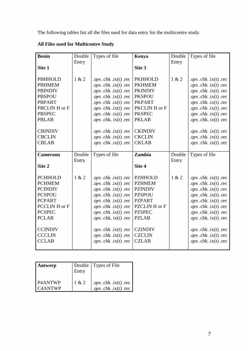
7
The following tables list all the files used for data entry for the multicentre study. All Files used for Multicentre Study Benin Site 1 PBHHOLD PBHMEM PBINDIV PBSPOU PBPART PBCLIN H or F PBSPEC PBLAB CBINDIV CBCLIN CBLAB
Double Entry 1 & 2
Types of file .qes .chk .ix(t) .rec .qes .chk .ix(t) .rec .qes .chk .ix(t) .rec .qes .chk .ix(t) .rec .qes .chk .ix(t) .rec .qes .chk .ix(t) .rec .qes .chk .ix(t) .rec .qes .chk. ix(t) .rec .qes .chk .ix(t) .rec .qes .chk .ix(t) .rec .qes .chk .ix(t) .rec
Kenya Site 3 PKHHOLD PKHMEM PKINDIV PKSPOU PKPART PKCLIN H or F PKSPEC PKLAB CKINDIV CKCLIN CKLAB
Double Entry 1 & 2
Types of file .qes .chk .ix(t) .rec .qes .chk .ix(t) .rec .qes .chk .ix(t) .rec .qes .chk .ix(t) .rec .qes .chk .ix(t) .rec .qes .chk .ix(t) .rec .qes .chk .ix(t) .rec .qes .chk. ix(t) .rec .qes .chk .ix(t) .rec .qes .chk .ix(t) .rec .qes .chk .ix(t) .rec
Cameroon Site 2 PCHHOLD PCHMEM PCINDIV PCSPOU PCPART PCCLIN H or F PCSPEC PCLAB CCINDIV CCCLIN CCLAB
Double Entry 1 & 2
Types of file .qes .chk .ix(t) .rec .qes .chk .ix(t) .rec .qes .chk .ix(t) .rec .qes .chk .ix(t) .rec .qes .chk .ix(t) .rec .qes .chk .ix(t) .rec .qes .chk .ix(t) .rec .qes .chk. ix(t) .rec .qes .chk .ix(t) .rec .qes .chk .ix(t) .rec .qes .chk .ix(t) .rec
Zambia Site 4 PZHHOLD PZHMEM PZINDIV PZSPOU PZPART PZCLIN H or F PZSPEC PZLAB CZINDIV CZCLIN CZLAB
Double Entry 1 & 2
Types of file .qes .chk .ix(t) .rec .qes .chk .ix(t) .rec .qes .chk .ix(t) .rec .qes .chk .ix(t) .rec .qes .chk .ix(t) .rec .qes .chk .ix(t) .rec .qes .chk .ix(t) .rec .qes .chk. ix(t) .rec .qes .chk .ix(t) .rec .qes .chk .ix(t) .rec .qes .chk .ix(t) .rec
Antwerp P4ANTWP C4ANTWP
Double Entry 1 & 2
Types of File .qes .chk .ix(t) .rec .qes .chk .ix(t) .rec

8
FLOW OF DATA THROUGH SYSTEM
A well-organized system for entry of questionnaire data on to computer is crucial for the success of the study. As the study is being carried out in four sites, it is especially important that each site adheres to the same procedures for data entry, checking, and back-up. If data is not entered on to computer in a systematic way, it is very easy for confusion to arise, possibly leading to loss of invaluable data or unnecessary duplication of work. An important role of the data entry team is to check carefully for missing data or incompatible responses. If these are found at the time of data entry, they can be re-checked by the data collection team as soon as possible. As shown on page 4, there are several different types of forms for the general population survey to be entered on to computer. These are the Household questionnaire (H) Individual questionnaire (I) Clinical examination form (C) Specimens form (S) Laboratory form (L) The titles of these forms are the same for the commercial sex worker survey (with the exception of the household questionnaire, which does not exist for CSWs). The flow of data through the system also applies for the CSW questionnaires, with the exception that there is no household questionnaire in this case. Each of the questionnaires and forms will be entered into a different computer file, as detailed on page 6. The individual questionnaire is the most detailed form and will take the longest to enter. Each site must ensure that the household questionnaire and other forms are also entered regularly (for example, set aside one day a week to enter data for these forms). For each of these types of forms, SIX boxes or files are needed to keep questionnaires/forms in at different stages of the data entry process. Thus for the general population a total of 30 boxes or files are needed. It is very important to have an ordered system of boxes or files in which to keep questionnaires/forms at the various stages of data entry. It is likely that boxes will be needed for the individual questionnaires, which are bulky, but files should be sufficient for the remaining forms. Each box or file is labelled with a letter and a number. The letter denotes the type of questionnaire or form, and the number denotes the stage in the data entry process that has been reached (see following details) e.g. Box C4 will contain clinical forms which have been entered onto computer once.

9
The process of data entry for the general population questionnaire is as follows: 1. Arrival of questionnaires for data entry a. On arrival, separate the questionnaire and forms into boxes labelled H1, I1, C1, S1, L1. Household questionnaires go into Box H1. Individual questionnaires go into Box I1. Clinical forms go into Box C1 Specimen forms go into Box S1 Laboratory forms go into Box L1 (for Kenya, lab forms are entered at a different site from the other forms). b. Use Tables H1-L1 to tick off the sticker numbers of each questionnaire and form which has arrived. (The final letter of the sticker number is not provided on these tables). 2. Check for missing information or mistakes a. Manually check each questionnaire/form in Boxes 1 for vital missing information (sex, age or line number). Check also for illegibility. b. If the questionnaire appears to be complete, put the questionnaires and forms into Boxes H2, I2, C2, S2, L2 respectively c. If there is vital missing information, obvious mistakes, or illegible responses, put the questionnaires and forms into Boxes H3, I3, C3, S3, L3. These are called the query boxes. 3. Return queries to supervisor a. Mark the sticker numbers of all questionnaires and forms in the query boxes (Boxes 3) with a Q on Table 1. b. The data entry supervisor should meet with the data collection supervisor weekly to discuss all the queries in Boxes 3. c. When queried questionnaires are returned for data entry, they go back into Boxes 1. Table 1 should be marked with a tick next to the query symbol Q. 4. First data entry a. Take questionnaires or forms from Boxes 2. b. Enter EPI-INFO c. In the Program option, go to ENTERX (This is the high memory version of ENTER and is necessary for data entry - do not use ENTER!)

10
d. Choose the appropriate file name P_____1.REC as shown on page 6 (e.g. PBHHOLD1.REC for household questionnaires in Benin), and choose ‘1’ for data entry. e. The questionnaire appears on the screen. Enter data from the questionnaire or form. The data entry program is set up to automatically skip questions which are not applicable, depending on previous responses. The program will automatically link the different data entry files if necessary (e.g. for information on spouses, or other sexual partners). At the end of one of these related files, you will be asked to press ‘Y’ or ‘F10’, and the program will then continue to prompt you for the remainder of the questionnaire. f. If there are no queries with the questionnaire or form, place it in Box H4, I4, C4, S4, or L4 after data entry. g. If there are queries with the information in the questionnaire, enter as much data as possible and circle the query on the questionnaire or form with a red pen. Then make a note of the query on the cover of the questionnaire or form. h. Place questionnaires with queries in Box 3 and mark the sticker number with a QE in Table 1 6. Second data entry It is important that all questionnaires and forms are entered twice onto computer by two different people. a. Take questionnaires from Boxes 4. b. Enter EPI-INFO and enter data into the relevant file P_____2.REC (e.g. PKINDIV2.REC for the individual questionnaire for Kenya). c. If there are no queries with the questionnaire, place it in Boxes H5, I5, C5, S5 or L5 after data entry. d. If there are queries with the information in the questionnaire, enter as much data as possible and circle the query on the questionnaire or form. Then make a note of the query on the cover of the questionnaire or form. e. Place questionnaires with queries in Boxes 3, mark Table 1 with a QE2. These questionnaires and forms will be returned to the data collection supervisor. 7. Filing of questionnaires The data has now been doubled entered on the computer and the questionnaires and forms need to be filed.

11
a. Take household questionnaires in box H5, sort into order of cluster number and household number, and file into Box H6. This box will contain all household questionnaires which have been double-entered onto computer. b. For each other type of questionnaires and form in Boxes 5, sort into order of sticker number. File into Boxes 6. 8. Back-up of computer files
Twice a day, at the end of each morning and afternoon, two copies of each REC file should be made onto separate backup floppy disks. These backup disks should be kept safely in a dry and dust-free environment (e.g. a plastic bag).
9. Validation of data entry The purpose of the double entry of the data is to pick up errors that have occurred during data entry. Checking for errors should take place twice - after the first 100 questionnaires have been entered, and finally, at the end of the study, i.e. when all general population questionnaires have been entered. Validation is carried out as follows: 1. Goto VALIDATE in the Program menu 2. The two file names are P______1.REC and P_______2.REC respectively (e.g. PCINDIV1.REC and PCINDIV2.REC to compare individual data for Cameroon). Carry out the validation for each of the 8 population REC files. When the commercial sex worker data has been entered, carry out the validation for the 3 commercial sex worker REC files. 3. Select output to printer 4. Press the space bar to select ‘Select unique ID’ 5. Move the cursor to select IDLABEL as the variable for ‘match field’ and press OK 6. The list of records which have discrepancies will be printed out. For each record, find the relevant questionnaire or form in Boxes 6 and edit the record (as detailed in point 6 below).

12
SPECIFIC POINTS FOR DATA ENTRY During data entry it is important that you note the following: 1. ENTERX
Because of the size and complexity of the main questionnaire for the individuals it is important that you choose the option ENTERX rather than ENTER in Epi-Info for entering the data.
2. Cluster and Household Number
For the Household and Individual questionnaire enter the 4 digit cluster number followed by the 4 digit household number to make an 8 digit number. This will be the unique identified of that household.
3. Missing Data
For all forms fill the field with 9’s for missing data. 4. Skips
To help with the data entry, some questions may be skipped automatically by the computer depending on the response. For example questions on spouses 2, 3 or 4 will be skipped for women as we assume they will currently have at most one husband.
5. Related files
As mentioned before the information on some forms is entered into more than one computer file. When this happens the computer will automatically link up to the necessary file.
6. Post-coding
Codes for some of the questions will only be devised after 100 forms have been collected. These are: Q206 (ethnic group), Q403 (type of relationship) and Q407 (ethnic group of sexual partner). Each person entering and checking data will need a copy of these additional codes once they have been devised. A copy should also be given to the interviewers and supervisors and a copy sent to Linda Williams or Helen Weiss at the London School of Hygiene and Tropical Medicine.
7. Editing data
To edit data which has already been entered (e.g. if a form is returned following a query) enter ENTERX, and choose the relevant EPI-INFO .REC file which is to be edited. 1. Type ‘1’ to enter data 2. Press CTRL-F 3. Type in the IDLABEL of the record you wish to edit 4. Press ENTER 5. Go to the field you wish to edit, type in the corrected data and press ENTER 6. When you have finished editing the data, press F10 to exit, and type Y to save the data.

13
Flowchart for data processing of questionnaires and forms
The box number will be prefixed by the letter referring to the type of questionnaire or form (H,I,C,S,L)
Return to supervisor
Arrival from data collection supervisor.
Record arrival of questionnaire or form on Table 1
Check manually for queries (missing data, inconsistencies)
BOX 4
BOX 1
BOX 2
BOX 3
Data entry into file P_____1.REC by first person
Queries
Queries
No queries
Queries
BOX 5
BOX 6
Data entry into file P_____2.REC by second person
No queries
No queries
Sort household questionnaires into order by cluster, household and line Sort other questionnaires and forms by sticker number

14
Appendix 2: The progress of a questionnaire The usual progress of the questionnaire and its data would be:
1. Interviewer collects data and completes questionnaire. 2. Interviewer checks questionnaire, and corrects any errors, returning to verify
data with the respondent if necessary. 3. Supervisor checks questionnaires, re-interviewing a sample of respondents. 4. A data entry clerk enters the data into the computer. 5. A different data entry clerk enters the data into the computer a second time. 6. The two data files are compared to find any typing errors, and errors are
corrected. 7. Either at the time of data entry, or afterwards, data are checked. The checks
ensure that data are within allowable ranges (e.g. sex must be either male or female). Checks also ensure that data are consistent from one question to another (e.g. if respondent is pregnant then sex must be female!). Any errors found are corrected.
8. When the data are clean, there will usually be a need to create new variables
or manipulate existing ones (e.g. calculation of latency periods, grouping age in five year bands etc.).
9. Data will need to be linked (or related) to data from other forms and
questionnaires (e.g. linking interview data with laboratory data). 10. Data may be exported for analysis by statistical, database, or spreadsheet
package. 1. Data Personnel As for field staff it is necessary to allow enough time for advertising and recruiting staff. It is also important to set out the terms and conditions clearly. When planning numbers and levels of staff required remember that there is more to do than just type in the data. Data entry staff are responsible for all the different tasks described in the data processing manual. Data Entry Clerks Unless trained coders/data entry clerks are already available, they will need to be hired and trained. The level of person hired depends on the extent to which they will be required to use their judgement. Byass (see refs) found that secondary school leavers could be trained for straightforward data coding and entry. Bourque and Clark (see refs) advise that, as the work of data processing personnel tends to be repetitive and tedious and demands attention to detail, it is important to explain during training the importance and relevance of their work to the whole research process. If open questions/qualitative
15
data are to be coded then it is generally necessary to employ data processing personnel with a higher level of education then completion of secondary school. The number of different tasks (such as those described in the data processing manual) that a data entry clerk will perform varies from study to study. Obviously a main component of a data entry clerk’s duties are to enter data and in order to estimate the amount of time needed for this it is obviously necessary to consider the amount of data. The number of characters for each questionnaire and form needs to be estimated (this is easier if you have draft or final versions). For the Gambian study of STDs in adolescents we estimated the following: • main questionnaire 150 characters • specimens form 15 characters • local laboratory form 40 characters • o/s laboratory form 30 characters Total 235 characters per respondent Assuming that 200 respondents will be interviewed per week and that data will be double-entered means that 200 x 2 x 235 = 94,000 characters need to be entered per week if the data processing is to keep up-to-date. Byass (see refs) estimated that secondary school leavers could be trained to enter around 50,000 characters per week. Therefore 2 data entry clerks would be needed to double-enter 200 forms per week. The sample size is 2000 so data entry alone would take 10 weeks. Having a minimum of 2 data entry clerks is a good idea if data are being double entered because then each clerk can do a single entry each. If trained keyboard operators are available they can enter data at much higher speeds. Data Manager / computer expert/ statistician etc. For large studies it is advisable to appoint a data manager who is responsible for ensuring that all the tasks described in the data processing procedures manual are followed closely by data entry clerks. This person can also the jobs which require a higher level of responsibility. For very large or complex studies it is worthwhile to bring in a specialist computer programmer or statistician. 5 Keeping track of the progress of data from an individual Tick lists Tick lists (or check lists) are invaluable to supervisors. They enable the supervisors and managers (as well as others involved with the study) to keep an overview of how data collection is proceeding. They are essential for keeping track of follow-up. Linking different forms In many studies there are several pieces of information collected for the same person. In order to link these pieces of information for each person a unique identifier for that person must be written or stuck onto every piece of information that relates to that person. The identifier (ID) often takes the form:
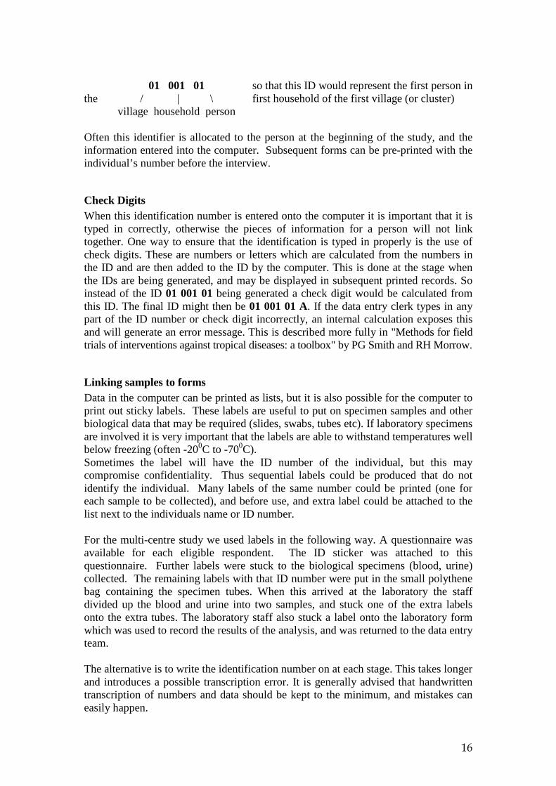
16
01 001 01 so that this ID would represent the first person in the / | \ first household of the first village (or cluster) village household person Often this identifier is allocated to the person at the beginning of the study, and the information entered into the computer. Subsequent forms can be pre-printed with the individual’s number before the interview.
Check Digits When this identification number is entered onto the computer it is important that it is typed in correctly, otherwise the pieces of information for a person will not link together. One way to ensure that the identification is typed in properly is the use of check digits. These are numbers or letters which are calculated from the numbers in the ID and are then added to the ID by the computer. This is done at the stage when the IDs are being generated, and may be displayed in subsequent printed records. So instead of the ID 01 001 01 being generated a check digit would be calculated from this ID. The final ID might then be 01 001 01 A. If the data entry clerk types in any part of the ID number or check digit incorrectly, an internal calculation exposes this and will generate an error message. This is described more fully in "Methods for field trials of interventions against tropical diseases: a toolbox" by PG Smith and RH Morrow.
Linking samples to forms Data in the computer can be printed as lists, but it is also possible for the computer to print out sticky labels. These labels are useful to put on specimen samples and other biological data that may be required (slides, swabs, tubes etc). If laboratory specimens are involved it is very important that the labels are able to withstand temperatures well below freezing (often -200C to -700C). Sometimes the label will have the ID number of the individual, but this may compromise confidentiality. Thus sequential labels could be produced that do not identify the individual. Many labels of the same number could be printed (one for each sample to be collected), and before use, and extra label could be attached to the list next to the individuals name or ID number. For the multi-centre study we used labels in the following way. A questionnaire was available for each eligible respondent. The ID sticker was attached to this questionnaire. Further labels were stuck to the biological specimens (blood, urine) collected. The remaining labels with that ID number were put in the small polythene bag containing the specimen tubes. When this arrived at the laboratory the staff divided up the blood and urine into two samples, and stuck one of the extra labels onto the extra tubes. The laboratory staff also stuck a label onto the laboratory form which was used to record the results of the analysis, and was returned to the data entry team. The alternative is to write the identification number on at each stage. This takes longer and introduces a possible transcription error. It is generally advised that handwritten transcription of numbers and data should be kept to the minimum, and mistakes can easily happen.
17
6 Quality control. Supervision of the quality of the fieldwork is crucial to ensure that the data are accurate. This can be done by a dedicated field supervisor, whose duties include monitoring the interviewers, clinicians, sample collection. Alternatively it can be done by the interviewers themselves, by checking and comparing answers on the questionnaires, finding discrepancies and going back to the respondents to clarify the response before they leave. Many studies use separate quality control (QC) questionnaires for this. These can be delivered by the supervisor, or by another interviewer blind to the first interview. Some studies insist that the QC responses are compared immediately and mistakes rectified, other studies are not able to compare responses until the end of the day, and it may be difficult to rectify mistakes. The data management strategy should outline how the QC questionnaires are used, by whom, and what will be done if discrepancies are found. The strategy should consider how respondents might feel about repeating the questionnaire or clinical examination. The duties of the supervisor may include: • Arrangements for transport - which clusters to visit on which day; • Checking where and when market days occur so that these can be avoided (as
many respondents may be absent from the household); • Greeting community leaders, informing them about the study and seeking their
cooperation; • Advising interviewers which households are eligible and keeping a checklist of the
outcome of each interviewers visit to each household; • Partial re-interviewing of a random sample of households already interviewed by
interviewers; • Spot checks that interviewers are following procedures; • Checking questionnaires and forms to ensure that they are completed properly; • Coordinating follow-up; • Handing completed questionnaires to data processing staff; • Answering queries by data processing staff; • Ensuring security and safety of interviewers; • Solving unanticipated problems (eg ineligible people asking to join the study);
18
2. Prepare data processing procedures manual This needs to set out all the procedures to be followed to ensure the quality of the data. It should include the following: • The flow of the questionnaires and forms from the field to final storage. For example
the field manager puts the questionnaires in box1 after they have been completed and he has checked them for legibility and completeness. After initial checking (and possibly some coding by data entry clerk or manager) this batch of questionnaires goes into box2. One data entry clerk takes these from box1, does the first data entry then puts them in box2 (after marking that they have been entered once). The second data entry clerk takes them from box2, does the second entry then puts the forms in box3. A clerk takes the forms from box3 sorts them into order and puts them in the final storage place. If anyone in this process has a query about any form, the query is marked and put in a special queries box for the field manager to pick up. Sometimes tick sheets are used to check which data has been received and where it is in the data entry process.
• How to use the data entry system set up according to section 3.4. Include lists of filenames, which computers will be used for first and second data entry, and in particular any merging needed.
• Procedures for entering data which has been corrected following discussions with field manager
• Taking backups (if you don’t do this you can lose the data!) • Running virus checking programs • Producing sticky labels • Producing lists or summary statistics to facilitate fieldwork (eg response rates, eligible
respondents needing follow-up etc.) • Responsibilities for maintaining hardware and software 7 Planning the computer resources and data sources Computing hardware If an institution’s computers are to be used rather than buying computers especially for the project you should check: • availability of equipment (time frames - other projects are likely to be using them as
well) • number and type of machines • are zip drives, USB drives etc. available to facilitate backup? • are up-to-date virus detection programmess installed? • what software is loaded, whether versions are the same on different machines • where they are located, i.e. all together in one room or spread out around building If you are going to buy new equipment, consider: • how many machines of which type are needed • requirements for other equipment - UPS, printer, zip drives, voltage regulators etc. • the time frame to order and ship the equipment
19
• customs regulations for import of equipment • what will happen to the equipment after the project has finished Computer software There are many specialist packages for different computing “jobs”. It is important to get the best software for each job. If different packages are used, it is usually easy to transfer the data from one package to another to do the next job. However this will involve the expense of buying more packages. • Databases (for entering, storing and manipulating data) eg dBASE, Access, FoxPro • Spreadsheets (matrices of numbers - useful for accounting and data manipulation) e.g.
Excel, Lotus • Graphics programs (for producing attractive plots and graphs - some of this can be
done from spreadsheets or statistics packages) e.g. Prism • Word Processors (for writing reports etc.) e.g. MS Word • Statistical packages (for statistical analysis of data) e.g. SPSS, SAS, Stata On this course we will use two packages: EpiData and Stata. 3. Data entry Design the data entry system You will be learning how to do this in detail during the Epi-Data sessions. The basic stages are: • Set up a data entry screen for the questionnaire and other forms • Set up range and consistency checks within the data entry screen • Enter the data • Check the data (this can be done by double data entry, manual checking of all data, or
manual checking of a random selection of data) • Clean the data (additional range and consistency checks (eg that there are no
laboratory forms for which there is no questionnaire etc.) • Merge the data (eg the data from the questionnaires with the different forms) • Recode the data (eg age into age groups) Facilitating computer data entry There are some further points to be considered in relation to transfer of the data from the questionnaire to a computer. Examples of different designs are attached to the handout. It is important to make clear which parts of the form are to be entered in the computer. This is usually done by providing boxes for each answer. It can useful to reserve the right-hand side of the form for "coding boxes". The questions, codes, written responses etc. are all put on the left-hand side and the coding boxes on the right are reserved for the numbers which are to be entered into the computer. This makes data entry and checking easier.

20
One box is needed for every digit. Hence, for each response you need to work out the maximum numbers of digits which may be needed. e.g. for height, what is the largest height that you are likely to record? Also, for a variable such as height, there may be a decimal point; indicate this between boxes on the questionnaire. The first few coding boxes of the questionnaire usually contain a code for the type of questionnaire, followed by identification codes for the respondent; typically, village (or community) code, household code, individual code. There may be some specific requirements for the way the data are to be recorded, depending on the software that it is intended to use. Consultation with data-processing staff and looking ahead to the requirements of the proposed analysis will help the design. Some computer packages cannot distinguish between a blank and a zero. This particular problem is becoming less common, but it needs to be considered when deciding on numerical codes e.g. code "missing values" as 9 rather than leaving a blank. Note that, except where questions are not applicable and have therefore been skipped, blanks should not be used for "not known" since they might be ambiguous for simply a missing value. 8’s are conventionally used to code “don’t know” Unless it is very obvious from the questionnaire a "code book" should be created so that during analysis the numeric can codes can be easily interpreted. Some packages allow notes to be attached to variables or datasets. This would be a useful way of ensuring that the 'codes' do not get lost Most computer software useful for this kind of data analysis uses short identifying names (usually up to 8 characters) for each variable. It is sensible to choose variable names that are indicative of the variable, (though an alternative is to call them by question number; Q1 and so on). It may be useful to put these variable names on the questionnaire itself. (Some computer software allows a longer name as well that will appear on the output but is not used in programming). Epi-Data, and some other packages enable the questionnaire to be reproduced on the screen, and the data to be entered through this medium. They also enable range and consistency checks to be built in to the entry process. This is called "direct data entry". For very small data sets (for example laboratory data) it may not be worth setting up a direct data entry screen and the data can be entered straight into a spreadsheet, or a word-processing package/editor, or may be downloaded from the laboratory machine (PCR for example). Keeping a master copy of the entered data. The data entry clerks will normally enter a small amount of data into a file. The file will be validated against a second entry of the same data. Each of the small files can then be added to a master file. It is usually for the data supervisor to keep this master file, and to add the data using a programme.
21
The master file can be named at the beginning of the study, so that programmes can be written for that data file. Programmes can be written not only to update (add) new data to the master file, but also to provide frequencies of the key variables. In this way study personnel can have up to date information about how many communities have been seen, the percentage of the target population that have been interviewed, the male-female split in the survey, etc. The programmes provide a record of what is happening to the data at that point in the study. 4. Cleaning data At this stage, the data is known to be an accurate reflection of the questionnaires (or other data collection device), but there may still be many mistakes. Cleaning the data is important to identify inconsistencies and mistakes. Data may be cleaned using the same software as data entry or in other software. If new software is being used, a direct translation of the master data must be used for the cleaning programmes. Cleaning programmes have two tasks. Firstly to identify potential mistakes, and secondly to rectify those mistakes. Examples of mistakes could be: • Inconsistencies missed by the data entry screen. • Impossible differences between two fields (eg. follow up date before the
recruitment date) • Inconsistent reports between two fields (eg. use of a condom by someone who
reports never having sex) • Identification problems (If a questionnaire exists for a subject who refused, or a
sample sticker label does not correspond with the list of subjects, or questionnaire numbers).
After the mistakes have been identified then a list can be generated. A data supervisor must then go over all the mistakes, compare them with the questionnaire and see if they can be solved. This is very time consuming and requires attention to detail. If the mistakes can not be rectified then the data will normally be assigned as missing. In most cases a programme is used to change the data and to clean the mistakes, this ensures that any changes are reproducible and verifiable. Keeping a master copy of the cleaned data. Once the data have been cleaned, a master copy of the cleaned data is kept. These clean data are the basis for the analysis, and can be used by others to examine different questions and hypothesis. These data may also provide the template for other future studies. The master data should be kept in the original format, and be translated into the software to be used for analysis (eg STATA or SAS). Once the master data have been put into the analysis format, a programme can be written to label all the variables and values in the dataset. Notes can be attached to explain any missing values, or other difficulties in the data.
22
5. Merging different data Only when the data are known to be clean can they be merged with other data from different sources. Before data can be merged another source of difficulty must be overcome. The variable on which the data are merged must match exactly. These problems should have been identified in the cleaning process, but if they have not, another iteration of cleaning may be required. It may be possible to merge data with some other datasets early on in the analysis. This will enable a partial analysis to be done. However other data may take longer to compile (eg from laboratory doing complex tests in another country). Thus a full analysis may not be possible until long after the data collection. Merging should be done using a programme in the analysis software. When merging new variables can be created, and possibly variables can be recoded to suit the analysis to be done. Categories can be obtained for age groups, or for the results of lab tests. By using programmes the master data are not altered in any way, and the analysis can be defined to answer the required question. Decisions may need to be taken over the ‘unit of analysis’ when merging data. If there is a hierarchy among the data which one corresponds to the unit of analysis. For example the data may include village based data, household based data, data on adults (mothers or children) and on children. Depending on the question being asked, and the hypothesis being tested, the unit of analysis may be the village, the household or the individual child.
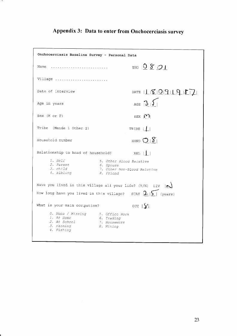
Appendix 3: Data to enter from onchocerciasis survev
Onchocerciasis Basel ine Surwey - personal Data
Date of rn terv :_ew
l a a i - .n Y s r J . r y g c t l - b
S e x ( M o r F )
T r i be (Mende 1 o the r 2 )
Household number
Have you l i ved i n t h i s v i - l l age a l t you r l i f e? ( y /N ) L IV l J
l { r r r ^ r I n n n l ' r : r t a l r n r 1 ' l - i - ' ^ ^ . i - t s L - . i ̂ , - . 1 r r ^ - ^
F \ -r r vw a \ J r J - v r r c r . vc l ou l i ved i n t h i s v i l l age? s rAy l L l> I ( yea rs )
What is your main occrpat ion? OCC f Vft - 4 - |
0 . l / o n e / M l s s i n q 5 . O f f i c e W o r k1 . A t l l ome 6 . T rad lnq2 . A t S c h o o f 7 . H o u s e w o r k3 . F a r m i n q B . M l n i n g4 . F i s h i n g
DNo rC r frrQat
DArE r ] - i f l rOrgt l*q_rLpr.-
A G E D f ) f
sEX [11
" P P r R t r l l It - l - l
HHN. Erffr
R e l a t i o n s h i p c o h e a d . o f h o u s e h o l d ? R E L f l f
1 . S e L f 5 . O t h e r B f o o d R e f a t i v e2 . P a r e n t 6 . S p o u s e3 . c h i f d 7 . O t h e r N o n - B l - o o d R e L a t t v e4 . s i b l i n g B . F r i e n d
23

Onchocerciasis Basel ine Survey - personal Data
Date of in terv iew
1 - ^ ; - .r I V E _ L 1 . r . y U d . r 5
S e x ( M o r F )
T r i be (Mende 1 O the r 2 )
Household number
rDNo rt rh r :1tL I
DArE r l r?r I r l r l r l tbrTi
,1 ,r r ( r b l l 1 2 l
HHNo t t tCt
acnl t r8r
sEX lfl
->Re la t i onsh ip t o head o f t r ouseho ld ,? REL l ) I
1 . s e l f 5 . o t h e r B f o o d R e l a t i v e2 . p a r e n t 5 . S p o u s e3 . c h i f d 7 . O t h e r N o n - B l o o d R e f a t t v e4 . s i b l l n q B . F r i e n d
Have you l i ved i n t h i s v i l l age a l t - you r l i f e? ( y /N ) L rV l t l t' + _ ,F T n t ^ r
- l n n a h r r r ar r vw r \ J r r y - r c r vc / o1 l - l ved i n t h i s v i r l age? s rAy i l i 3 f ( yea rs )
t ^71 - ^F - . i ̂wnar l _s you r marn occupa t ron? OCC l_ l
0 . l / one / M i ss ing 5 . O f f i ce Work1 . At l lome 6. Trad ing2 . A t Schoo l 7 . I l ousework3 . F a r m i n q B . M i n i n q4 . F i s h i n q
24
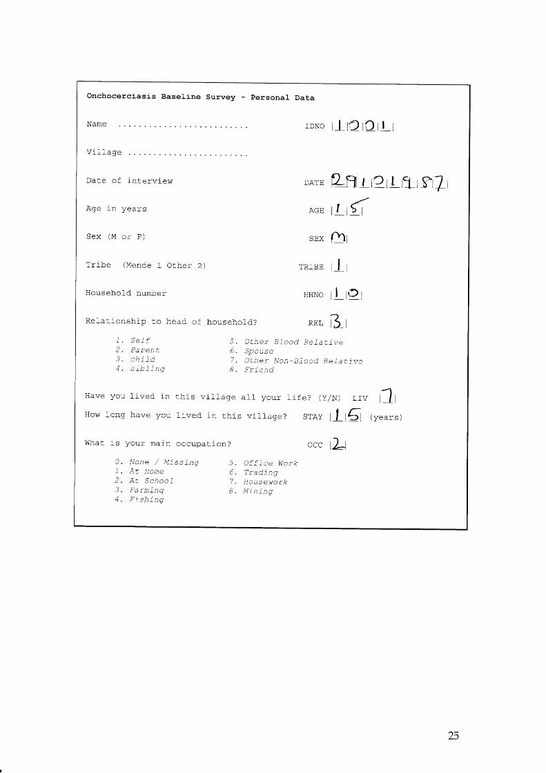
Onchocerciasis Basel ine Surwey - personal Data
r D N o t I t 2 i C t l t
Date o f i n te r v rew
r a a . . i - ^n y s r r r y e d l - b
S e x ( M o r F )
T r i be (Mende 1 O the r 2 )
Househol-d number
Re la t i onsh ip t o head o f househo ld?
DArE Zff | f?rt t l_rtr/r, y '
A G E I I l > |
sEX lli
T p r R E , I il r l
H H N o l l t a t
REL i3 rr . a = L L
2 . P a r e n t3 . c h i f d4 e l h l i n n
5 . O t h e r B l - o o d R e _ l a t i v e6 . S p o u s e7 . O t h e r N o n - B l o o d R e f a t i v eB . F r i e n d
Have you l i ved i n t h i s v i l l age a l f you r l i f e? ( y /N ) L rV f l f
T]nr^r - l
nn c l .r r r rar r vw r \ J r r v r r c r vc l ou i i vec r i n t h i s v i r l age? s rAy l l f S ( yea rs )
What is your main occupat ion? occ la0 . l / o n e / U i s s i n q 5 . O f f i c e W o r k1 . A t l l ome 6 . T rad lng2 . A t S c h o o f 7 . I l o u s e w o r k3 . F a r m i n q B . M i n l n q4 . F i s h i n q
25
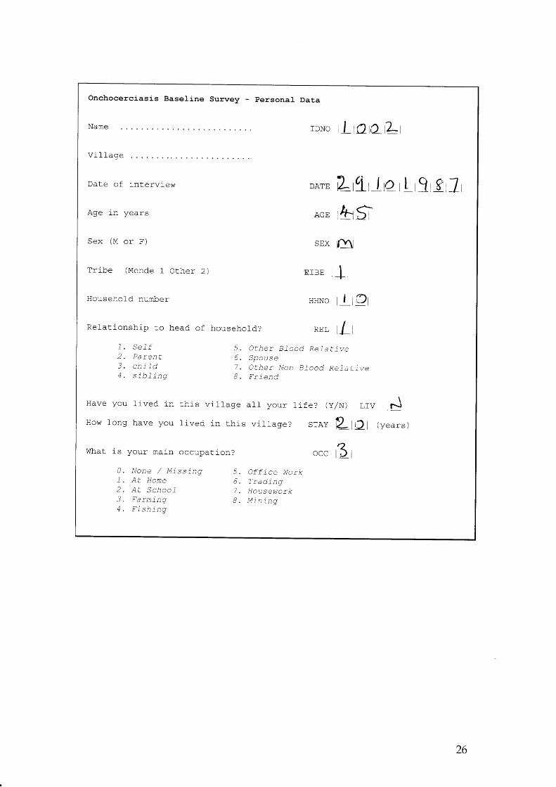
Onchocerciasis Basel ine Survey - personal Data
rDNo lL tC lL lL t
Date o f i n te r v i ew
r * a - . 1 *n v c : r r r y e d I s
S e x ( M o r F )
T r i be (Mende 1 O the r 2 )
Household number
DArE L f t t l t 2 t I i g t t t l r
AGE th$
sEX m
lprP,tr I I Ir - + I
HHNO t I tQt
Re la t i onsh ip co head o f househo ld? REL I L t
1 . S e _ Z f 5 . a t h e r B l o o d R e _ l a t i v e2 . P a r e n t 6 . S p o u s e3 . c h i l d 7 . O t h e r N o n - B f o o d R e f a t t v e4 . s i b J i n q B . F r i e n d
Have you l i ved . l n t h i s v i t t age a t l you r t - i f e? ( y /N ) L r v I J f
lT . r r^r I nnrr rn: r rar r v v v l v r a y r r a v c | o L l l - i v e d i n t h i s v i l l a g e ? s r A y L t C l ( y e a r s )
What is your main occupat ion? occ r3 r0 . l , / one / t t i ss inq 5 . O f f i ce Work1 . A t l l ome 6 . T rad inq2 . A t S c h o o f 7 . I l o u s e w a r k3 . F a r m i n g B . M i n i n g4 . F i s h i n g
26

Onchocerciasis Basel ine Survey - personal Data
rDNo iC tS tC tA
Date of in tervrew
I - ^ ; . ^nv c : _Lr ] y gc t l . : i
s e x ( M o r I , )
T r i be (Mende 1 O the r 2 )
Household number
Re la t i onsh ip t o head o f househo ld?
D A r E t t t L C r l r l r g r S i T r
AGE lztLl
asEX l f I
m n r n - t L-Lr t_Lnr1 | | |
HHNo lQlS I
D F r II+
1 . S e - l f2 . P a r e n t3 . c h i f d4 . s i b T l n q
5 . O t h e r B l o o d R e - Z a t i v e6 . S p o u s e7 - a t h e r N o n - B f o o d R e f a t l v e
a ! l g l l u
Have you l i ved i n t h i s v i t l age a t l you r 1 i f e? ( y /N ) L rV f Y f
l T n r ^ r I n n n h : r r ar rvw r \J r ry r .Lo.ve |ou l - ived in th is v i l tage? srAy f 2 .+1f (years)
Whac is your main occupat ion? occ l5la . l J o n e / U i s s i n q 5 . O f f i c e W o r k1 . A t l l ome 6 . T rad ing2 . A t S c h o o f 7 . I t o u s e w o r k3 . F a r m i n q B . M l n i n q4 . F i s h i n q
27

Onchocerciasis Basel ine Survey - personal Data
Date o f i n te r v rew
n ^^ ; . ^f l 'v c _Lrr y cct.L 5
What is your main occupac ion?
0 . l / o n e / t t i s s l n q 5 . O f f i c e W o r k1 . A t l l ome 6 . T rad ing2 . A t S c h o o l 7 . H o u s e w o r k3 . F a r m i n g B . M i n l n q4 . F i s h l n g
rDNo f Cf t tCr l r
Sex ( tu o r F) sEX f f i
r r ibe (Mende 1 orher 2 ) rRrBE f I f
Househord number HHNo f L f Kf- ? - '
IRe la t i onsh ip co head o f househo l_d? REL I \ o I
1 . S e l f 5 . O t h e r B l o o d R e _ Z a t i v e2 . p a r e n t 6 . S p o u s e3 . c h i f d 7 . O t h e r N o n - B l - o o d R e f a t t v e4 . s i b J i n g B . F r i e n d
\Have you l i ved i n t h i s v i l l age a l l you r l i f e? ( y /N ) L IV I n - , I
L { n r ^ z l n n n h a r r a \ / A r 1 ' l ; - ' ^ . l - . 1 - f l - . . j ^ - - - . 1 r r ^ - ^ - f l {* vw l v ray r ravu l ou l i ved i n t h i s v i r l age? s rAy ? - t> l ( yea rs )
DArE r l rs tQqr j r?nf t
AGE ]!f 1f
occ 5r
28
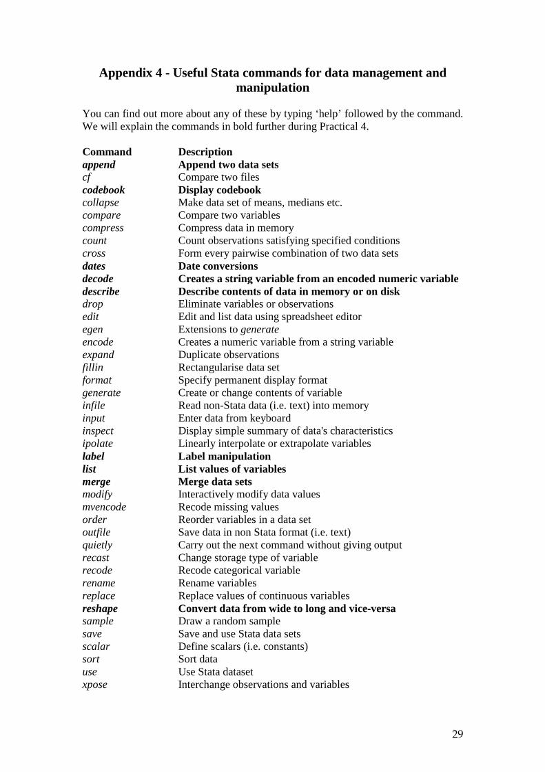
29
Appendix 4 - Useful Stata commands for data management and manipulation
You can find out more about any of these by typing ‘help’ followed by the command. We will explain the commands in bold further during Practical 4. Command Description append Append two data sets cf Compare two files codebook Display codebook collapse Make data set of means, medians etc. compare Compare two variables compress Compress data in memory count Count observations satisfying specified conditions cross Form every pairwise combination of two data sets dates Date conversions decode Creates a string variable from an encoded numeric variable describe Describe contents of data in memory or on disk drop Eliminate variables or observations edit Edit and list data using spreadsheet editor egen Extensions to generate encode Creates a numeric variable from a string variable expand Duplicate observations fillin Rectangularise data set format Specify permanent display format generate Create or change contents of variable infile Read non-Stata data (i.e. text) into memory input Enter data from keyboard inspect Display simple summary of data's characteristics ipolate Linearly interpolate or extrapolate variables label Label manipulation list List values of variables merge Merge data sets modify Interactively modify data values mvencode Recode missing values order Reorder variables in a data set outfile Save data in non Stata format (i.e. text) quietly Carry out the next command without giving output recast Change storage type of variable recode Recode categorical variable rename Rename variables replace Replace values of continuous variables reshape Convert data from wide to long and vice-versa sample Draw a random sample save Save and use Stata data sets scalar Define scalars (i.e. constants) sort Sort data use Use Stata dataset xpose Interchange observations and variables

30