Epi 222

Lecture 4 - Too many statistics in too little time….

Copyright © 1999-2001 Leland Stanford Junior University. All rights reserved.Warning: This presentation is protected by copyright law and international treaties. Unauthorized reproduction of this presentation, or any portion of it, may result in severe civil and criminal penalties and will be prosecuted to maximum extent possible under the law.

Statistics and HRP 222

This is not a statistics course and neither is 223.

In 223 I will tell you the “requirements” and “assumptions” for a few statistics but I will not provide you with the reasons why these requirements exist.

If you would like to learn more statistics, read the books books that follow.

Great Statistics and Epidemiology Books

How to lie with Statistics by Huff the closest thing to a Platonic perfect first text in statistics

Statistics (3rd edition) by Freedman et al. This is the best “real” statistics book I have read. It will help

you develop intuition about how common statistics really work.

Epidemiology: Study design and data analyses by Woodward easily the best practical book on Epidemiology

Biostatistics: The Bare Essentials by Norman, Streiner excellent breadth of topics for epidemiology and biostatistics,

wonderful to read.

Great Statistics and Epidemiology Books(2)

Common Statistical Methods for Clinical Research with SAS examples by Walker a cookbook which tells you how to do common statistics

Survival Analysis using the SAS System by Allison an awesome applied survival book, it needs a second edition

Survival Analysis : A Self-Learning Text by Kleinbaum. excellent introduction which is more theoretical than Allison

Logistic Regression using the SAS System by Allison. a very good applied logistic regression book

Other Useful Books

Matricies of Statistics (2nd edition) by Healy If you must do the math underlying the statistics and

math is not your first language, get this.

Categorical Data Analysis Using the SAS System (2nd edition) by Stokes et al.. This is the bible for doing categorical analyses in SAS.

While not bad, it does not read easily.

An Introduction to Categorical Data Analysis by Alan Agresti. This is the second or third book you want to read on

categorical data analysis. It is excellent but not for amateurs.

Inferences

You want to emphatically state that you know whether or something is true about a population. You can be testing a hypothesis or

estimating a value.Typically, you can not test every

person in the population so you take a sample and hope that you can infer back to the population.

What You Need to Do Is….

Descriptive statisticsrates, frequencies

Inferential statisticsTest for statistical differences between

groups.Measure the strength of the associations.Model relations between variables.

What Measure?

Critical factors determining your statistic How many outcome measures are used?

Are you looking to predict a variable or describe the relationship between two outcome measures?

What scale is the outcome measured in?Binary (yes/no) , nominal (red, green, blue), ordinal

(small, medium, large)Are you looking at counts or percentages?

How many predictor variables are you using? What scale are the predictors measured in?

Binary Predictor and Outcome

If you have a binary predictor and a binary outcome a logical way to summarize the data is by looking at it in a contingency or cross tabulation table.

The “cross tab” is measured by rows and columns (r * c).

Analyzing Categorical Data

When data is in a 2x2 table, you can get lots of useful statistics with no effort: Chi-Square Fisher's exact McNemar's Odds ratios Relative risks Mantel-Hanszel for Stratified Tables

Proc Freqdata pox; input exposure $ spots $ @@; datalines;

lots yes lots yes lots yes lots yes lots no little no lots yes lots yes lots yes little no lots no lots yes little yes little no lots yes lots yes lots no little no lots yes lots yes lots yes little no lots no lots yes little no lots no little no lots yes; run;proc freq; tables spots*exposure;run;*bad;proc freq; tables exposure*spots;run;*less bad;

Proc Freq Again (2)

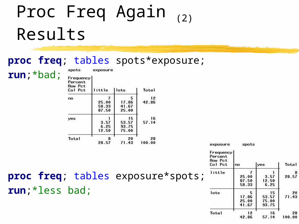
Results proc freq; tables spots*exposure;run;*bad;

proc freq; tables exposure*spots;run;*less bad;

Proc Freq Again (3)

Formatted Rightproc format; value $yn 'yes' = ' Spotted' 'no' = 'No Spots'; value $exposure 'lots'=' lots'

'little'='little';run;proc freq order=formatted; format spots $yn. exposure $exposure.; tables exposure * spots;run; /* best*/

More exposure

Worse outcome

Proc Freq Again (4)

Formatted Right Plus Stats!

Once the data is in the right format, getting analyses is easy.

You just add:/ chisq to the tables

statementtables exposure * spots / chisq;

Proc Freq Again (5)

Results

Which chi square?Typical Person2

Two ordinal variablesYates or Fisher are used for small expected value Left = cell 1,1

less than expected

Used for modelingAsymptotically equivalent to Person

Proc Freq Again (6)

With Expected

You can see the expected values that it is worried about:

/ chisq expected;

Measures of Agreement

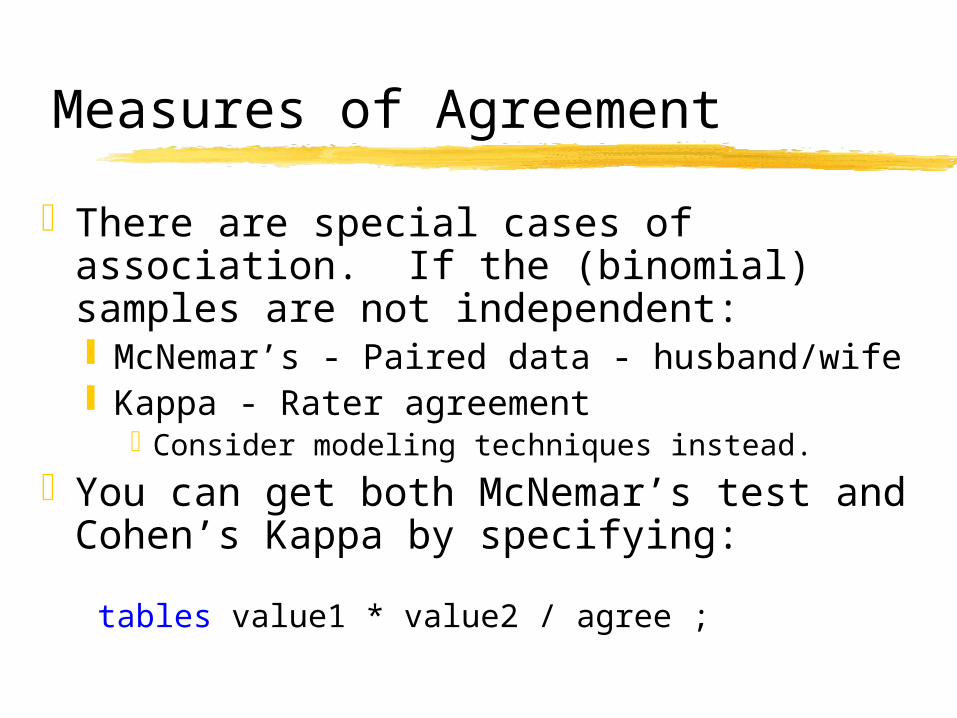
There are special cases of association. If the (binomial) samples are not independent: McNemar’s - Paired data - husband/wife Kappa - Rater agreement

Consider modeling techniques instead.

You can get both McNemar’s test and Cohen’s Kappa by specifying:tables value1 * value2 / agree ;

Strength of Association

Now that you have shown a relationship, what about the typical epidemiology techniques to assess strength of association? Odds Ratio

You can always calculate an odds ratio. Relative Risk

Is a measure of association appropriate for retrospective studies when the outcome of interest occurs less than 10% of the time?

the ratio prevalence in column 1 for row1/row2

Odds Ratio / Relative Risk

To see the OR and RR add:

/ measures;

This is just an odds ratio. If this were a retrospective study….

These are relative risks:If the “bad thing” is in the left column then use col1 risk

Importing a Table

data bigspot; input exposure $ health $ count @@; datalines; exposed diseased 66 exposed healthy 24 notExp diseased 38 notExp healthy 56

; run;

You can import data by weighting it:

proc freq data = bigspot; weight count; tables exposure*health / nocol nopct chisq;run;

Importing a Table (2)

Results

SAS 8.x Output

Differences in Mean

Does a mean differ from a constant? One sample t-test

Assumptions• Normally distributed data.

Do two means differ? Two sample t-test

Assumptions• Equal variance for groups you are comparing.• Normally distributed data.

One Sample t-testdata fakeIQ;

input scores @@;datalines;

106 95 89 92 121 100 91 104 98126 76 71 103 84 107 65 117 110 103;run;proc ttest data = fakeIQ h0 = 100 alpha=0.1;

var scores;run;

proc univariate data = fakeIQ normal;var scores;

run;

The null hypothesis is that average IQ is 100.

Generate 90% confidence intervals.

Check for normality.

One Sample t-test (2)

Two Sample T-test

The for a two sample t-test is simple also

proc ttest data = grace.analysis;class pih_a;var dsl_insuli;

run;

Two Sample T-test (2)

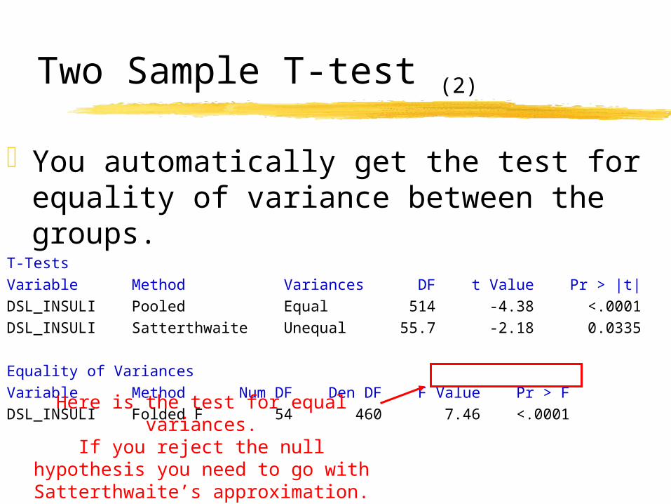
You automatically get the test for equality of variance between the groups.

T-TestsVariable Method Variances DF t Value Pr > |t|DSL_INSULI Pooled Equal 514 -4.38 <.0001DSL_INSULI Satterthwaite Unequal 55.7 -2.18 0.0335

Equality of VariancesVariable Method Num DF Den DF F Value Pr > FDSL_INSULI Folded F 54 460 7.46 <.0001

Here is the test for equal variances.If you reject the null hypothesis you need to go

with Satterthwaite’s approximation.

Two Sample T-test (3)

proc univariate data = grace.analysis normal;var dsl_insuli;histogram;

run;

Here you reject the null hypothesis of normality.

Test --Statistic--- -----p Value------Shapiro-Wilk W 0.501456 Pr < W <0.0001Kolmogorov-Smirnov D 0.316378 Pr > D <0.0100Cramer-von Mises W-Sq 21.96289 Pr > W-Sq <0.0050

Wilcoxon

If you can not go with a T-Test you can consider its non-parametric analog Wilcoxon Rank-Sum Test.

It is also simple syntactically:proc npar1way wilcoxon data=grace.analysis;class pih_a;var dsl_insuli;

run;

Three or more Groups

When you need to compare three or more means you will probably want to do an ANOVA. ANOVA is implemented in several procedures. Simple ANOVAs can be done with proc univariate. I recommend that you try to use proc anova – it

is designed to be easy to use and covers most experimental designs.

If you can’t do proc anova you can always use proc glm.

Practical Stats - ANOVA

proc sort data = gad; by dosegrp; run; proc univariate data = gad;by dosegrp; var hama;

title 'One-Way ANOVA'; title2 'Walker EXP. 5.1: HAM-A Scores GAD'; run; proc glm data = gad; class dosegrp; model hama = dosegrp; means doesgrp/t duncan hovtest=levene; run;

Linear Regression and Correlation

You may be interested in finding out if two variables vary together. That is, as one variable goes up in value does the other variable go up also. Alternatively you may want to know if as one goes up does another go down.

Typically people are interested to find out if there is a linear relation between the variables.

You can produce scatter plots with the SAS regression procedures or SAS graph.

Proc reg has lots of features for plotting regression lines, confidence intervals and residuals.

The SAS graph procedure gplot is designed to produce high resolution scatter plots. It has lots of features to make photo-ready graphics.

Scatter plots

Scatter with Proc Reg

You can get a scatter plot from proc reg like this:

proc reg;format nphs 2. educate 2.;symbol1 v = dot;model nphs = educate;plot nphs * educate;* plot nphs * educate / pred;* plot r.*nqq.;

run;

Scatter with gplot

This looks lousy:proc gplot data = blah;format nphs 2. educate 2.;label nphs = "blah";symbol1 v = + font = swiss;plot nphs * educate ;

run;

Scatter with gplot

goption reset;axis1 order=(0 to 20) label=(angle=90 rotate=0) minor=none;

axis2 order=(0 to 20) label=("Yrs Education") minor=none;

goption vsize = 7in hsize = 7in;proc gplot data = blah;format nphs 2. educate 2.;label nphs = "blah" font = "swiss";symbol1 v = + font = "swiss";plot nphs*educate/vaxis=axis1 haxis=axis2;

run;quit; axis1; axis2;

Got the Jitters?

With data like this which has lots of over-plotting, it is useful to add a little bit of jitter to each point. This spreads the values out so you can tell about how many values are at each location.

This process is called jittering. data blah2;set blah;nphs2 = nphs + ranuni(0);educate2 = educate + ranuni(0);

run;

goption reset;axis1 order= (0 to 20) label=(angle = 90 rotate = 0) minor=none;

axis2 order= (0 to 20) label=("Yrs Education") minor=none;

proc gplot data = blah2;format nphs 2. educate 2.;label nphs2 = "Jittery people in Household" font = "swiss";label educate2 = "Jittery Yrs of Education";symbol1 v = + font = "swiss";plot nphs2*educate2/ vaxis=axis1 haxis=axis2;

run;quit;axis1;axis2;

Coefficients

If you need a Pearson correlation coefficient:

proc corr data = grace.analysis ;

var dsl_igf dsl_insuli;

run;This is the correlation coefficient.

This is the p-value.

Add the word spearman here for his correlation.

Evaluating a Regression

You will undoubtedly want to know how good your regession fit is.

You can have sas plot residuals and predicted values: plot r.*p. / vref =0;

You can output datasets with predicted and/or residual values:proc reg data = blah;model outcome = predictor;output out=newData p=thePred r=theRes ucl= up lcl = low;

run;

Homework

Update your virus definitionsScan for virusesSend it to balise@stanford.eduMake sure to include comments

explaining what you are doing.