Environmental Modeling

Steven I. GordonOhio Supercomputer Center

sgordon@osc.eduJune, 2004

Environmental Models Offer Many Options

• Many models– Atmospheric processes– Hydrologic processes– Ecological systems– Natural hazards– Many interactions

• Many scales– Local habitats– Regional – mesoscale– Global

Problems in Instruction

• Modeling complex, dynamic systems

• Changes occur both spatially and temporally

• Quality of data to confirm model validity often questionable

• High degrees of uncertainty

• Many different processes cross disciplinary boundaries– Challenge for students with varying background

– Challenge for faculty trying to apply to instruction

Mixed Approaches

• Models based on physical theory– Fluid dynamics

– Mechanics

– Biochemistry

• Models based on statistical and empirical estimates– Used to simplify the complex dynamic systems

– Based on abstractions that do not always apply

Many Places Many Parameters

• Requirements for data describing initial conditions at each place in the model– Amount of data required dependent on model scale

– Data acquisition difficult

– Increasing availability of spatial data from public sources

• Most models embed many parameter choices– Values found under different circumstances

– Calculated based on different principles

• Choices can make model use decisions dizzying

Basic Model Components

• State variables describing status as different places at time zero

• Flow over time and space of matter, energy, organisms

• Transformation of physical, chemical, or biological characteristics over time

Alternative Representations

• What governs the movement from one place to another?

• How does movement vary with changes in environmental conditions? How is this change represented (steady steady, stochastically, statistically)?

• How will space be represented – implicitly, one, two or three dimensions?

First Example – Dissolved Oxygen in a Stream

• Measure of health – ability to support diverse ecosystem

• Basic relationship– Inversely related to temperature– Range between 0 and 14 ppm (mg/l)

Conceptual model

• Organic waste (BOD) decomposed by bacteria that use oxygen– DO=f(1/BOD)

• Two processes– Deoxygenation– Reaeration

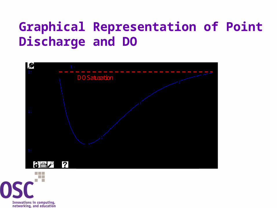
Graphical Representation of Point Discharge and DO

10:09 AM Sun, Apr 11, 2004

Dissolv ed Oxy gen of Sugar Creek

Page 1

0.00 6.25 12.50 18.75 25.00

Day s

1:

1:

1:

4

6

8

Dissolv ed Oxy gen: 1 -

1

1

1

1

DOSaturation

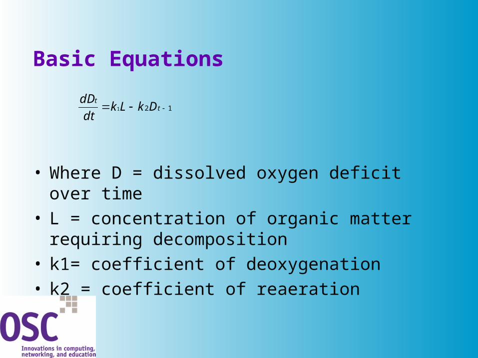
Basic Equations

• Where D = dissolved oxygen deficit over time• L = concentration of organic matter requiring

decomposition• k1= coefficient of deoxygenation• k2 = coefficient of reaeration

121 tt

DkLkdt

dD

Stella Model Example

Excel Engineering Version

• Qual2K• Based on EPA code for DO called Qual2E

• http://www.epa.gov/athens/wwqtsc/html/qual2k.html

• Example run

Complexity of the Model

• Choose which aspects to focus on• Leave the rest as a “black box”• Create an exercise that focuses on variables

of interest– E.G. BOD load; sensitivity to reaeration parameter

and temperature

Simple Point Source/Receptor Model

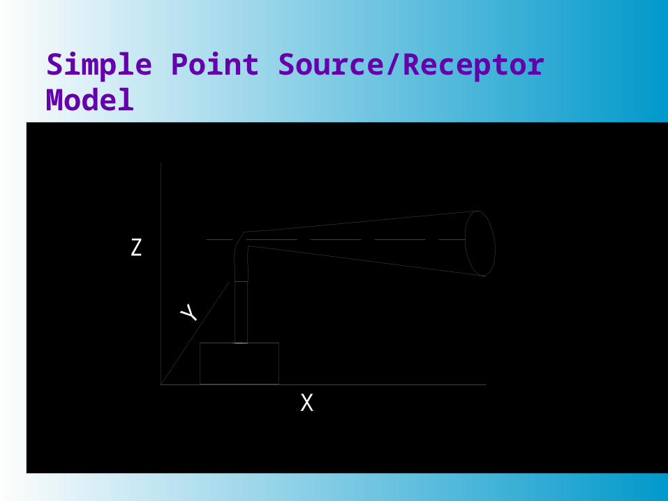
Simple Point Source/Receptor Model

Z

X

Y

Simple Point Source/Receptor Model

h

h

H

VirtualOrigin

PlumeCenterline

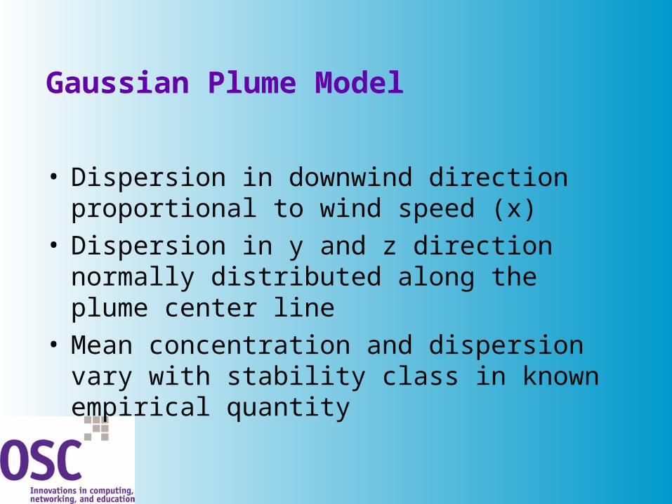
Gaussian Plume Model

• Dispersion in downwind direction proportional to wind speed (x)

• Dispersion in y and z direction normally distributed along the plume center line

• Mean concentration and dispersion vary with stability class in known empirical quantity

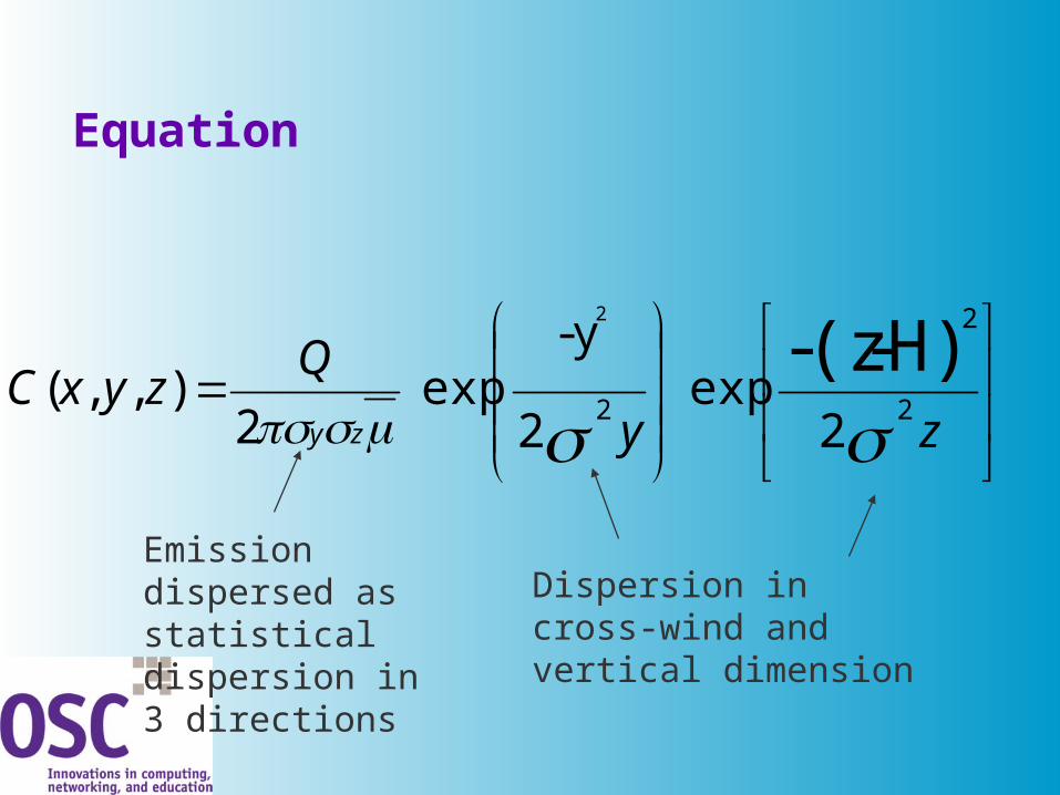
Equation

zy

QzyxC

zy 2

2

22

exp 2

y-exp

2),,(

H)-(z-2

Where:

C (x,y,z) = concentration of pollutant in 3 dimensions given steady state emission

X = horizontal distance from source in direction of wind vector and along plume centerline

Y= horizontal distance perpendicular to and measured from the plume center line

Z= vertical distance from ground to plume center lineQ= mass rate of production of pollutant over time

Where:

Ū = mean wind speed in the x direction

H = effective height of plume

direction wind-crossin deviation standard y

PCL fromdeviation standard vertical z

Equation

zy

QzyxC

zy 2

2

22

exp 2

y-exp

2),,(

H)-(z-2

Emission dispersed as statistical dispersion in 3 directions

Dispersion in cross-wind and vertical dimension

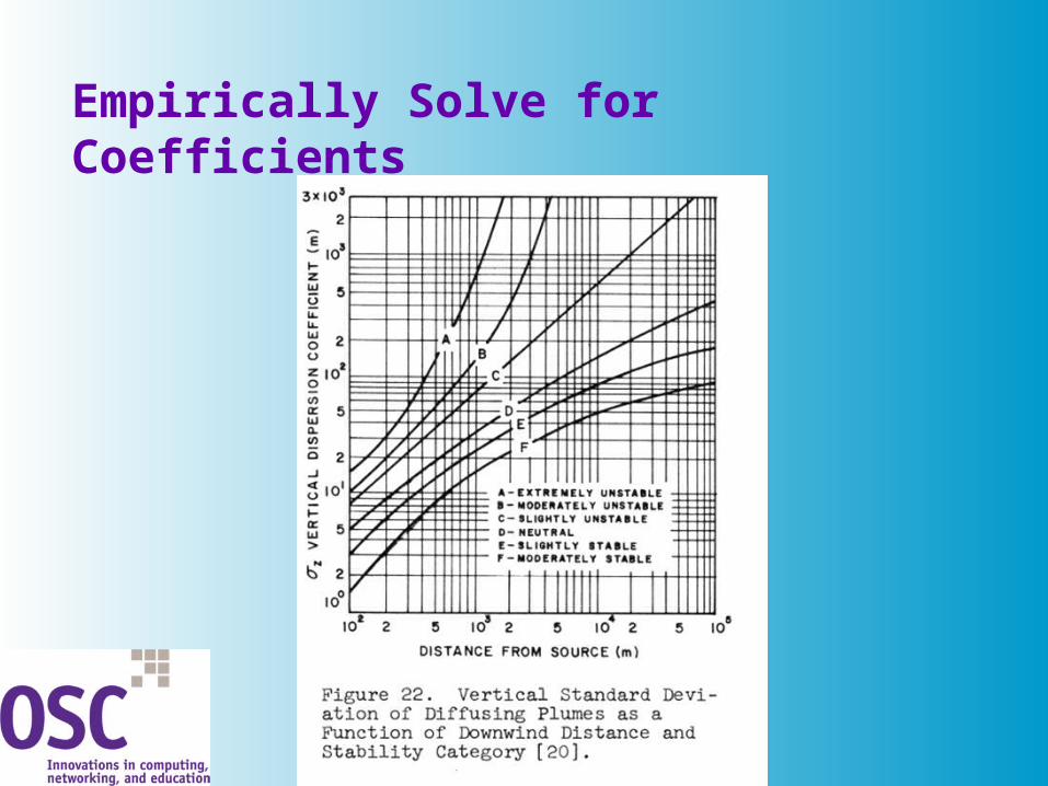
Empirically Solve for Coefficients

Solving the Equation

• Probability distribution of different wind speed, direction, stability class occurrence

• Solve the model for each condition• Weight the answer by the frequency of each

condition

Stability Wind Rose

Excel Version of the Model

The Climatological Dispersion Model

Alternative Approaches

• Find a simple version of a model to run in Stella or a spreadsheet

• Have students add to the simple model by taking advantage of the documentation/discussion in more complex models

• Run a more complex model but vary only a few variables most relevant to the class topics

Create and Test a Set of Exercises

• Regardless of approach – need to carefully prepare instructions that include:– Readings on the model basis– Step-by-step instructions– Realistic scenarios– Clear list of expected exercise outcomes– Opportunities for feedback

Sources of Information

• See attached sheet with web links to a variety of modeling and data sites