1

IMPERIAL COLLEGE LONDON

Faculty of Engineering

Department of Chemical Engineering

Environmental Impact Assessment And

Optimization Of Urban Energy Systems

By

Nicole C. Papaioannou

A report submitted in fulfilment of the requirements for the PhD

October 2012

2

ABSTRACT

Over the last century, the world has witnessed rapidly increasing urbanization trends.

Consequently, the urban governments of this époque require the measure and

monitoring of their cities’ expansion, as well as the impacts that this development has

on the environment, the economy and the society. The energy sector in particular,

plays a determining role in maintaining acceptable conditions in all these domains.

The concept of sustainable development appears to combine a number of disciplines,

which assess it in different manners. This research attempts to show how a

combination of methods can provide further insight to a city’s energy system. More

specifically, the concepts of life cycle assessment and mixed-integer optimization are

brought together and applied to a hypothetical urban energy systems case study

looking at three different environmental impacts: global warming potential, resource

depletion and air quality. The model chooses the types of energy technologies that are

most suitable when aiming to minimize each environmental impact, showing that a

carefully selected energy systems design can perhaps achieve lower overall

environmental impact within an urban area. Life cycle assessment, material flow

analysis and ecological footprint methodologies are further performed on two case

studies: a UK eco-town and the city of Toronto. Five energy technology scenarios are

compared based on these environmental impact assessment methodologies and

conclusions drawn as to which scenario achieves the lowest values. Attention is drawn

to stakeholder involvement and how interpretation of environmental impact is

“vulnerable” depending to which priorities are set.

3

KEYWORDS

Urban energy systems; environmental impact assessment; optimization;

I declare that the work found in this thesis is my own and that all else is appropriately referenced.

‘The copyright of this thesis rests with the author and is made available under a Creative Commons

Attribution Non-Commercial No Derivatives licence. Researchers are free to copy, distribute or

transmit the thesis on the condition that they attribute it, that they do not use it for commercial purposes

and that they do not alter, transform or build upon it. For any reuse or redistribution, researchers must

make clear to others the licence terms of this work’

4

ACKNOWLEDGEMENTS

First of all, I would like to thank my supervisor, Prof. Nilay Shah of the Centre for

Process Systems Engineering at Imperial College, for his invaluable support and

guidance during the course of this research. I am very grateful for the time and insight

I was provided with, to successfully complete this work. I consider myself very

fortunate to have had such a helpful, friendly and inspiring supervisor. I am very

thankful to have been given this novel and fascinating topic and thus, allowing me to

make a (small) contribution to the long-term BP UES project.

Secondly, I would like to thank my parents for their priceless and irreplaceable

encouragement during the last few (but not only) years. Mom, without your

motivating words and the faith in me that you expressed on a daily basis, none of this

would have been realised to the optimum extent. All I can say is that you have set the

bar very high with your own achievements, and I am trying to catch up - this work

only brings me another step closer.

5

TABLE OF CONTENTS

TABLE OF CONTENTS .............................................................................................................. ABSTRACT ...................................................................................................................................... 2 ACKNOWLEDGEMENTS .............................................................................................................. 4 LIST OF FIGURES .......................................................................................................................... 7 LIST OF TABLES ............................................................................................................................ 8

1. INTRODUCTION .............................................................................................................. 9 1.1 Urban evolution .................................................................................................................... 9 1.2 Cities as eco-systems: the history and concept of urban metabolism ............. 13 1.3 Background to this Work ................................................................................................. 13

1.3.1 The Synthetic City Toolkit ..................................................................................................... 15 1.4 Aims and Objectives .......................................................................................................... 18

2. LITERATURE REVIEW ................................................................................................ 21 2.1 Precedents of Similar Work ............................................................................................ 21

2.1.1 Systems Optimization Coupled with LCA ........................................................................ 21 2.2 Early studies of urban metabolism .............................................................................. 35 2.3 Introducing the Case Study: The UK Eco-Town ........................................................ 39 2.4 City Footprints ..................................................................................................................... 40 2.5 Optimization Solution Techniques ............................................................................... 46

2.5.1Mixed-Integer Programming ................................................................................................. 46

3. METHODOLOGY ........................................................................................................... 50 3.1 Data Processing ................................................................................................................... 50 3.2 Environmental Impact Assessment Methods ........................................................... 52 3.3 Material Flow Analysis ..................................................................................................... 53

3.3.1 MFA re-named ............................................................................................................................ 54 3.4 Ecological Footprinting .................................................................................................... 57

3.4.1 Calculating the ecological footprint of an energy system ......................................... 58 3.5 Life Cycle Assessment ....................................................................................................... 59

3.5.1 Cultural theory of risk and LCA ........................................................................................... 64 3.6 A hypothetical case study ................................................................................................ 66

3.6.1 Model notation and formulation ............................ Error! Bookmark not defined.

4. RESULTS AND ANALYSIS ........................................................................................... 71 4.1 Input data and assumptions ........................................................................................... 71 4.2 Optimization results .......................................................................................................... 72 4.3 LCA-based Scenario Analysis .......................................................................................... 73 4.4 Selecting EIA methodologies for UES design ............................................................ 75 4.5 Scenario Analysis ................................................................................................................ 76

5. DISCUSSION ................................................................................................................... 85 5.1 Life cycle assessment ........................................................................................................ 86 5.2 SimaPro software ............................................................................................................... 87 5.3 Material flow analysis ....................................................................................................... 87 5.4 Urban metabolism .............................................................................................................. 88 5.5 Ecological Footprints......................................................................................................... 88 5.6 Simplistic Approach ........................................................................................................... 89

6

5.7 “Which EIA methodology (or combination of methodologies) is most relevant and appropriate to the design of a particular UES and how easily can it be applied”? ................................................................................................................................. 90 5.8 What do these results mean to policy-makers? ....................................................... 91

6. CONCLUSIONS ............................................................................................................... 93 6.1 Recommendations for Future Work ............................................................................ 95

7. REFERENCES.................................................................................................................. 97

8. APPENDICES ................................................................................................................ 105 8.1 Appendix A – Input data used in the GAMS model ............................................... 105 8.2 Appendix B – Calorific values per fuel ..................................................................... 114 8.3 Appendix C – Input data for Eco-town ...................................................................... 114

7

LIST OF FIGURES

Figure 1 Changes in the world's urban and rural population, projected to 2030

(UNDESA, 2006) ........................................................................................................... 9 Figure 2: The forecast on how the world primary energy demand is expected to

change by 2030 (IEA, 2004). ....................................................................................... 11 Figure 3: World primary energy demand by fuel in the New Policies Scenario, 1980 to

2035 (IEA, 2011). ........................................................................................................ 12 Figure 4: Shares of energy sources in world primary energy demand by scenario, 2035

(IEA, 2011). ................................................................................................................. 12 Figure 5: Framework of Synthetic City modelling toolkit (UES Annual Report, 2010).

...................................................................................................................................... 16 Figure 6: The objective of minimizing only output emissions of the conventional

VCM process is in fact sub-optimal (Stefanis, 1995). ................................................. 22 Figure 7: Avoiding allocation by enlargement - expanding the boundaries (Azapagic

& Clift, 1999). .............................................................................................................. 24 Figure 8: Non-inferior curve for ulti-objective optimization (Azapagic & Clift, 1999).

...................................................................................................................................... 27 Figure 9: Optimal trade-off results for the case study (Hugo et al., 2005). ................. 31 Figure 10: The urban metabolism of Brussels, Belgium in the early 1970s

(Duvigneaud and Denaeyer-De Smet, 1977). .............................................................. 38 Figure 11: The UK eco-town. ...................................................................................... 39 Figure 12: Comparing the city to a large animal to portray the concept of the

ecological footprint (Wackernagel and Rees, 1996: 228). ........................................... 41 Figure 13: The global overshoot of the ecologican footprint over the Earth's

biocapacity from 1988 onwards (Global Footprint Network, 2007). .......................... 45 Figure 14: The structure for the model, depicting the connections between system,

emissions and damage categories. ............................................................................... 51 Figure 15: The Eco-Indicator 99 methodology (Pre Consultants, 2001). SPM =

suspended particulate matter, VOC = volatile organic compoun, PAH = polycyclic

aromatic hydrocarbons, HCFC = hydrofluorocarbons. ................................................ 63 Figure 16: The relative environmental impact of urban energy systems of a UK eco-

town based on greenhouse gas emissions per capita (LCA) and ecological footprint

per capita. ..................................................................................................................... 80 Figure 17: Location of Toronto and its census metropolitan area in the province of

Ontario (Wikipedia, 2012). .......................................................................................... 81 Figure 18: Total Greenhouse gas emissions for the city of Toronto ............................ 83 Figure 19: The ecological footprint for each energy scenario for the city of Toronto 84

8

LIST OF TABLES

Table 1: CO2 emissions created by the direct combustion of different fossil fuels, i.e.

Scope 1 emissions, (Emission factors calculated on a Net Calorific Value basis ),

(Defra, 2011). ............................................................................................................... 59 Table 2: Energy technologies and their approximate capacities based on author

estimates. O&M = operating and maintenance costs. .................................................. 71 Table 3: Changes in environmental impact values when minimizing one objective at a

time. ............................................................................................................................. 73 Table 4: The model's choice of technologies according to environmental impact.

Values indicate the per cent of total urban energy demand satisfied by a given

technology. CHP = combined heat and power............................................................. 74 Table 5: Material needed to run the UK eco-town based on five different scenarios. 78 Table 6: Material needed to run the city of Toronto based on five different scenarios.

...................................................................................................................................... 82 Table 7: Heat and electricity demands per cell number ............................................. 111 Table 8: Calorific Values used for the scenario building ..........................................114

9

1. INTRODUCTION

1.1 Urban evolution

Over the last 100 years, the world population has experienced quickly increasing

urbanization trends. These trends are only expected to maintain an upward

trajectory in the coming decades. The drivers of this expansion vary and can be

functions of the demographic, economic, social and political evolution of the

world’s metropolises. The fact remains that the global fraction of urban

population rose from only 13% in 1900, to 49% in 2005 (UNDESA, 2006).

Moreover, according to recent United Nations population projections, 60% of the

world’s population is expected to live in cities by 2030, amounting to 4.9 billion

urban dwellers, as shown by Figure 1 below.

Figure 1 Changes in the world's urban and rural population, projected to 2030 (UNDESA,

2006)

10

Parallel to this urban blossom, the definition of sustainable development started to

emerge and has encouraged urban governments to quantify a city’s performance

in those terms. The “Brundtland Report” (UNWCED, 1987) defined sustainable

development as “meeting the needs of the present without compromising the

ability of future generations to meet their own needs”. In order to satisfy this

definition, urban governments are looking for ways to measure the state of their

city and evaluate its improvement against any desired targets. Targets such as

reducing the environmental impact of an urban area are extremely common.

Naturally, the energy sector plays a pivotal role in the attempts to achieve

sustainable development. Fossil fuels are seen as a “capital” resource that depletes

over time, whereas renewables may be viewed as energy “income” to the planet

(Hammond 2007). It has been estimated that 75% of global energy consumption

occurs in cities and 80% of greenhouse gas emissions is due to cities in some way

(UN Habitat, 2007). Approximately half of this amount results from the burning

of fossil fuels in cities for urban transport and the other half arises from energy

use in buildings and appliances - both these practices being necessary for

maintaining the human quality of life in urban systems. Indeed, climate change,

sustainable development and urbanization go hand-in-hand. Global energy

demand forecasts shown in Figure 2 estimate an increase of primary energy

demand of 60% in the next three decades as developing countries industrialise and

rich countries continue to consume power (IEA, 2004).

11

Figure 2: The forecast on how the world primary energy demand is expected to change by

2030 (IEA, 2004).

In the 2011 World energy outlook, the IEA expects the most important changes to

be in the patterns of energy generation and production. The use of all fuel types

develops, yet fossil fuels are expected to still be responsible for more than one-

half of the overall primary energy demand increase, even under the New Policies

Scenario. Traditional and modern renewable energy increases its share from 13

per cent in 2008 to 18 per cent in 2035, and nuclear energy appears to grow from

6 per cent to 7 per cent of total primary energy demand.

12

Figure 3: World primary energy demand by fuel in the New Policies Scenario, 1980 to 2035

(IEA, 2011).

If indeed the global panels take significant action to stabilise greenhouse gas

concentrations at 450 ppm, these trends will further be enhanced. Under the 450

ppm Scenario, global coal use falls from approximately 27 per cent of the global

mix to around 16 per cent by 2035. Generally in this scenario, world use of fossil

fuels falls rapidly, while low-emission sources of renewable and nuclear energy

blossom.

Figure 4: Shares of energy sources in world primary energy demand by scenario, 2035 (IEA,

2011).

13

Given that urbanization and energy demand go hand-in-hand, and rising numbers

are expected in both, a better understanding of urban energy systems is at the

forefront of urban government agendas.

1.2 Cities as eco-systems: the history and concept of urban metabolism

Cities can be thought of as having a metabolism, like plants or animals. Studies on

the concept of urban metabolism have been conducted since 1965, investigating

water trends, materials, energy and nutrient flows within cities. Typically cities

have exhibited increasing per capita metabolism with respect to water,

wastewater, energy and materials over time. Through these studies, metabolic

processes that potentially put the sustainability of cities in danger can be

pinpointed. These include changing ground water levels, depletion of local

materials, regular and irregular accumulation of toxic materials and nutrients, and

effects such as the summer urban heat island. By understanding urban

metabolism, urban policy makers are to better comprehend the extent to which

local resources are approaching exhaustion and hence, devise relevant strategies

to delay exploitation. The fact is that urban metabolism studies have not been

produced for enough cities worldwide and ideally, more are required.

1.3 Background to this Work

The research topic under investigation is part of the BP Urban Energy Systems

(UES) project, which is taking place at Imperial College London in collaboration

with BP. The UES project is trying “to document and understand in detail how

14

energy, people and materials flow through a city [and] to show how the efficiency

of both existing and new-built cities can be radically improved” (BP, 2006).

Energy systems have been defined as the “combined processes of acquiring and

using energy in a given society or economy” (Jaccard, 2005). This short

description can be interpreted in a variety of ways within an urban setting, such as

the analysis if physical flows in a small neighbourhood (Thomas, 2003) or when

taking the approach of social scientists and policy makers, it can become the study

of how these flows are affected by “town-planning, environmental goal-setting,

employment policies, and so on” (Alexandre et al., 1996). For the BP UES

project, these and additional views are considered in order to “identify the benefits

of a systematic, integrated approach to the design and operation of urban energy

systems” (Shah et al., 2006).

The energy systems modelling approaches used in the UES project are suitable for

estimating future urban demands for energy services and possible infrastructures.

These approaches provide opportunities to consider more efficient use of energy

as well as alternative technologies.

This project aims to investigate the energy balances observed in urban systems in

terms of resources entering a city and wastes leaving, and estimating the

environmental impact of activities associated with these inputs/outputs. These will

15

form part of the wider study into sustainable and highly efficient future urban

developments.

Surprisingly, not enough is known on how cities consume energy, impact the

environment and whether the way energy is used is optimal. Together with other

components, a huge part of this project is dedicated to the development of the

Synthetic City toolkit, which models urban energy systems.

1.3.1 The Synthetic City Toolkit

The Synthetic City (SynCity) platform (Keirstead et al., 2009) was developed by

a group of researchers within the BP UES project at Imperial College, as a toolkit

for the modelling and optimization of energy systems within the urban

environment. It comprises three major components, a layout model, an agent

activity simulation model and the resource technology model.

16

Figure 5: Framework of Synthetic City modelling toolkit (UES Annual Report, 2010).

A brief description of the major components follows:

The layout model

As its title suggests, the layout model is used to optimize the spatial design of the

city based on cost, energy reduction and environmental or other parameters. The

input is in the form of GIS geographical data on the existing city infrastructure

and it is utilized to optimize the location of additional facilities of interest (such as

residential, commercial and other buildings).

The agent activity model

This stochastic sub-model provides an estimate of the daily demand-generating

activities of individuals within a city, such as the annual average passenger-

kilometres for travel, as well as resource demands over time and within each zone

17

of a city. This gives rise to spatial and temporal energy demand patterns, forming

the output of the model.

The Resource-Technology Network (RTN) Model

This final sub-model of SynCity is used to explore different scenarios for the

optimal provision of energy to cater for the demand patterns generated by the

agent activity model.

Conceptually the model splits up the city into smaller cells, of any size or shape

and they do not need to cover the full area within certain city borders. Each of

these cells stands for a dynamic entity within the models, with its own resource

demands, resource conversion and storage technologies. Additionally, there can

be connections between individual cells for the transportation of resources, plus

external connections for bringing in or sending out resources. Resources can

represent any material or energy resource that is consumed or generated,

including wastes (e.g. CO2, waste water, waste heat, refuse, etc.). Resource

demands that arise in each cell must be satisfied, by converting other resources,

transporting those resources from other cells, importing them from outside the

city, or taken up from a storage, if there is availability of that resource.

The model developed in this work can constitute a part of the RTN model in the

SynCity framework, since the type of results obtained can complement

performance measures (e.g. GHG emissions) that form a part of it.

18

1.4 Aims and Objectives

This project targets to investigate the energy balances observed in urban systems

in terms of resources entering a city and wastes leaving, and estimating the

environmental impact of activities associated with these inputs/outputs. These will

form part of the wider study into sustainable and highly efficient future urban

developments.

The broad aim of this research is to provide a set of methodologies and tools for

the planning and operation of urban energy systems using the Life Cycle

Assessment (LCA) concept, modelling and optimization techniques. It is based on

detailed analyses and studies of urban environments, the various processes within

them and some application of appropriate modelling and optimization

formulations to reveal the trends and behaviour of urban energy systems.

This report starts with a concise literature review, covering relevant pieces of

work performed by other researchers in the field and follows with a description of

the methods used to facilitate this project. The work covered describes the

emissions inventory and the applications of the LCA methodology in a simple,

hypothetical urban energy systems case study. Subsequently, it is shown how

modelling frameworks inspired by natural ecology can help us valuate the

sustainability of urban energy systems as applied to a UK eco-town. After first

discussing the similarities between cities and ecological systems, a review of

19

relevant environmental impact assessment methods is presented before

demonstrating how these methods can be combined with optimization techniques

to assess the life-cycle impacts of an urban energy system. Finally, the discussion

ties together the results and considers what they reveal in the broader context of

urban energy systems.

The rationale for choosing a UK eco-town as a case study lies in the fact that

much of the data was readily available since this eco-town has been a popular

object of research at Imperial College.

There is a large amount of energy-related data available from international

organizations such as the IEA, the World Bank, the OECD, as well as, from

academics that have looked into material and energy flow analysis (e.g. Schulz,

2005). Currently, work is being done at Imperial College on providing an

enhanced idea of the way that urban energy systems operate at Energy Futures

Lab, also under the BP UES project and so this research will form a useful

complement.

Taking the above into consideration, the research question for this investigation

has been set as:

“Which EIA methodology (or combination of methodologies) is most relevant and

appropriate to the design of a particular UES and how easily can it be applied”?

20

This thesis has been structured as follows:

Chapter 2 contains a concise literature review relevant to this field of work;

Chapter 3 describes the approach and methodology to this study;

Chapter 4 presents and analyses the results;

Chapter 5 discusses the findings of this research;

Chapter 6 provides the concluding remarks and recommendations for future

work;

Chapter 7 gives the list of references used throughout this work.

21

2. LITERATURE REVIEW

2.1 Precedents of Similar Work

2.1.1 Systems Optimization Coupled with LCA

Various authors have attempted to incorporate LCA within a formal process

systems optimization framework, with the Methodology for Environmental

Impact Minimization (MEIM) being one of the earliest attempts, performed by

Stefanis et al. (1995). The authors highlight the need to account for the waste

associated with INPUTS to a process (upstream wastes associated with raw

materials, energy generation, etc.) and not solely the OUTPUTS. The MEIM is

illustrated using a case study of VCM production. As such, the methodology

involves three steps: (i) definition of the system boundary (expanded to include

raw material extraction and energy generation), (ii) environmental impact

assessment, where for each pollutant released from the process, a vector denoting

its corresponding environmental impact (air and water pollution, solid wastes,

global warming, photochemical oxidation and stratospheric ozone depletion) can

be obtained leading to an aggregated impact vector, and (iii) synthesis of a more

environmentally benign process, where the incorporation of the environmental

impact criteria in process optimization takes place in order to find the best plant

design that achieves both minimum global environmental impact and minimum

economic cost.

22

A significant result that arose from Stefanis’ work is the fact that when only local

emissions are minimized, the minimum global impact is not necessarily achieved.

Through his VCM case study, it is shown that the Zero Avoidable Pollution

(ZAP) approach is not always the best environmental choice. (refer to Figure 6)

Figure 6: The objective of minimizing only output emissions of the conventional VCM

process is in fact sub-optimal (Stefanis, 1995).

According to Stefanis, “a minimum site-specific discharge limit exists beyond

which the global environmental impact increases due to trade-offs in waste

generation over the whole life cycle”.

23

Azapagic & Clift (1995) brought LCA and Linear Programming (LP) together in

order to environmentally optimize a product system. The problem lies in how the

allocation of environmental burdens such as resource depletion, emissions, solid

waste, etc., in a system with more than one product should take place. By

representing the whole productive system through a LP model and solving

through its marginal1 and shadow values, the environmental performance of the

product system can be analyzed and managed. The authors first identify the

environmental burdens and then aggregate them into different impacts such as

greenhouse effect, ozone depletion, etc. Weights are then assigned to the impacts

according to their importance (based on environmental and socio-economic

objectives that are of interest to the decision-makers) and the shadow values are

used to identify products and activities in the system which make the greatest

contribution to the overall environmental impact. LP accounts for the different

states of the system and multi-objective LP helps to resolve conflicting demands

on system performance.

The same authors further refined their work (Azapagic & Clift, 1999) to

incorporate the issue of how to allocate burdens between different inputs to the

system/systems which produce more than one functional output, as well as to

reflect both the use and production of recycled materials. Still by using marginal

allocation of environmental burdens based on physical causality, the authors

propose either the avoidance of allocation through system boundary expansion or

1 Infinitesimal, small variations about existing operations that are always linear.

24

solution based on the real behaviour of a product system, i.e. its causal

relationships. System expansion can be illustrated by an example taken by

Azapagic & Clift (1999). If System I produces products A and B and System II

produces only product C, and A is to be compared with C, then allocation can be

avoided by broadening the system so that an alternative way of producing B is

added to System II. (refer to Figure 7)

Figure 7: Avoiding allocation by enlargement - expanding the boundaries (Azapagic & Clift,

1999).

The comparison now takes place between System I producing A + B and Systems

II and III producing C + B.

A

B A

B B

C

C

+

25

The methodology includes linearization of the process model to relate the total

burdens in the system to the material and process properties through marginal

allocation coefficients and minimizing environmental burdens at the Inventory

level of the LCA and environmental impacts at the Impact Assessment level.

Optimization is proposed at the Improvement Assessment level. By using three

examples of systems (multiple input, multiple output and multiple use) marginal

analysis reveals whether the environmental burdens are process or material related

and possible places for system improvement. Marginally allocated burdens also

depend on how the system is operated and not just on the internal structure of the

system. The authors criticize their work by stating that detailed data on sub-

processes must be available to establish the type of causality and that marginal

allocation cannot always be used to describe average or discrete changes (which

may be non-linear) in a system.

Through their work in 1999, Azapagic and Clift introduce the concept of coupling

LCA and Multi-objective Optimization (MO), thus establishing the link between

environmental impacts, operation and economics of the system. A general MO

problem of a system can be stated with the following relationships (Azapagic &

Clift, 1999):

Minimize f (x, y) 1[ f , pff ,...2 ] (2.1)

26

s.t.

h (x, y) = 0

g (x, y) ≤ 0 (2.2)

x XRn

y YZq

where f is a vector of economic and environmental objective functions; h (x, y) =

0 and g (x, y) ≤ 0 are equality and inequality constraints, and x and y are the

vectors of continuous and discrete variables, respectively. The equality constraints

may be defined by energy and material balances; the inequality constraints may

describe material availabilities, heat requirements, capacities, etc. A vector of n

continuous variables may include material and energy flows, pressures,

compositions, sizes of units etc., while a vector of q integer variables may be

represented by alternative materials or processing routes in the system.

The system is first optimized on each objective to identify the feasible regions,

while other functions are ignored. One of the functions is then arbitrarily chosen

as an objective function and all other objectives converted to constraints. A

number of optimizations, in which the RHS of the objectives-constraints are

varied within the feasible region, are performed to yield a range of non-inferior

solutions. With this methodology, objectives do not have to be aggregated into a

single objective and the Best Practicable Environmental Option (BPEO) and Best

Available Technique Not Entailing Excessive Cost (BATNEEC) can be

27

identified. The advantage of this technique is that multi-objective optimization in

environmental system management in the LCA context offers a set of alternative

options for system improvements, rather than a single optimum.

The case study used to illustrate LCA and MO is a system that produces five

boron products. MO was performed on three objectives: total production (P), costs

(C) and Global Warming Potential (GWP). Results are shown in Figure 9 below:

Figure 8: Non-inferior curve for ulti-objective optimization (Azapagic & Clift, 1999).

Points A and G represent optimum values of GWP and P respectively. At point A,

GWP is at a minimum, but so is production. By moving away from A, along the

non-inferior curve, both GWP and total production increase and at G, production

is at a maximum and GWP also increases. Additionally, the costs also increase

from A to G by an average of 20%. Clearly, all points on the non-inferior curve

are optimal in a Pareto sense and decision makers can select any solution from A

28

to G, depending on how much of one objective they are prepared to give up in

order to gain another. If all objectives are considered of equal importance, then

one of the possible ways to choose the best compromise solution is to identify the

operating conditions at which all objectives differ from their optima by the same

percentage. In that case, it would be the solution at point C. However, if some

objectives are considered more important than the others, any other solution on

the non-inferior curve can be chosen as the best compromise.

When referring to a Pareto optimum, it is implied that no individual can be made

better off without making at least one other individual worse off. In this case, the

Pareto or non-inferior surface is optimal in the sense that none of the objective

functions can be improved without worsening the value of some other objective

function.

As a follow-up to her previous work, Azapagic (1999) presented LCA and its

application to process selection, design and optimization as a powerful decision-

making tool for more sustainable performance of process industries. The

methodology is given as follows:

Carry out a LCA study

Formulate MO problem in LCA context

MO on environmental & economic criteria

Multi-criteria decision analysis and choice of best compromise solution

29

The way to reach the choice of best compromise solution is to optimize the

system on a number of objective functions so that optimum solutions are found on

the Pareto surface. The choice of environmental objectives to be optimised

depends on the Goal and Scope of the study. Thus, optimisation can be performed

either at the Inventory or Impact Assessment levels, in which case the

environmental objectives can either be burdens or impacts. Therefore, local and

global system improvements are found by first moving the system conditions on

the Pareto surface, and then moving along it. Since all objectives on the surface

are Pareto-optimal, certain trade-offs between the objectives are needed to

identify the best compromise solution.

The above methodology is illustrated using the examples of BPEO for SO2, NOx

and VOC abatement, where it is concluded that the choice of BPEO depends on

the boundaries, the operating state of the system and on the background economic

system in which it operates. In addition, it is shown that from an environmental

point of view, minimization of output emissions only as normally carried out in

conventional system optimization, can lead to suboptimal solutions. The author

further identifies the limitation that the LCA approach assumes that the

environmental burdens and impacts functions are linear, i.e., they are directly

proportional to the output of functional unit(s) and that there are no synergistic or

antagonistic effects.

30

Hugo et al. (2004) present a process design methodology for identifying

opportunities where step-change improvements in both process economics and

environmental impact can be achieved by using multi-objective optimisation

techniques. The approach extents the previously developed MEIM for process

selection. Accepting that a conflict between economic and environmental

concerns inherently exists, the task is to modify a process through the use of

alternative materials. Extensions to the MEIM methodology include the explicit

formulation of new environmental performance criteria, and a multi-objective

optimization algorithm based upon a domination set strategy for detecting Pareto

optimality. Their work uses liquid-liquid extraction operations as an example to

show how the full plant-wide integration of alternative materials satisfies both

environmental and economic performance.

One year later, Hugo et al. (2005) investigate the viability of a hydrogen economy

by applying multi-objective optimization techniques to the strategic planning of a

hydrogen infrastructure. Their model is based on the fact that hydrogen can be

manufactured by a variety of primary energy feedstocks and distributed in a

variety of forms using different technologies. The question they are aiming to

answer is what are the most energy efficient, least damaging yet most cost

effective pathways to deliver hydrogen to the consumers?

Again, a conflict of objectives arises since the most profitable infrastructure is not

necessarily the least environmentally damaging. Therefore a set of trade-off or

31

Pareto solutions, and not just a single solution, exist, lacking a one, “best”

alternative.

Figure 9: Optimal trade-off results for the case study (Hugo et al., 2005).

The case study depicted in Figure 9, is based on a geographical region with six

production sites identified for potential installation of central production

technologies. Thereafter, the demand for hydrogen was forecasted for each city. It

can be seen that at one extreme of the curve, the maximum Net Present Value

(NPV) solution and the corresponding infrastructure choice can be found. At the

other extreme, the minimum GHG emissions solution with its corresponding

infrastructure choice can be found. Moving along the trade-off curve, from one

32

extreme to the other involves a series of alternative infrastructure design and

investment strategies, all of which are perfectly feasible.

Azapagic et al. in their more recent work (2007) attempt to identify options for

reducing the total environmental footprint of human activities in urban areas,

rather than shifting environmental impacts from area to area or from one life cycle

stage to another. A hypothetical city with 500,000 inhabitants is used as an

example to map the flows of pollutants in the urban environment. The authors

integrate LCA, Substance Flow Analysis (SFA), Fate and Transport Modelling

(F&TM) and Geographical Information Systems (GIS) to achieve the

aforementioned. The methodology is described below:

Spatial definition of sources in GIS

Definition of sources using a combined LCA-SFA methodology

Quantification of burdens/impacts at source using the LCA-SFA

methodology

F&TM and quantification of the environmental impacts at the receptor end

for mapping in GIS

The authors highlight the importance of ensuring that the reduction of pollution in

the urban environment is not carried out at the expense of “other” environments.

One of the advantages of this methodology is that, while it focuses on the urban

environment, it also helps to understand wider environmental implications.

33

In the most recent developments of energy systems optimization, Liu et al. (2009)

have presented a paper on multi-objective optimization of polygeneration energy

systems. This new technology involves the co-production of electricity, synthetic

liquid fuels, but also hydrogen, heat and chemicals in one process, while

promising low emissions. In this work, economic and environmental factors are

optimised simultaneously, showing a variety of likely technology combinations

and types of equipment. The model is formulated as a non-convex mixed-integer

nonlinear programming problem and the optimal Pareto trade-off curves are

produced using global optimization tools and parallel computation techniques.

Research by Keirstead et al., (2009) on evaluating integrated urban biomass

strategies for a UK eco-town showed that by increasing the integration of energy

services, e.g. through the use of combined heat and power systems, improves the

efficiency of urban energy systems. The particular eco-town is supplied with heat

and power from biomass sources in this case. Results show that even though

biomass offers a promising low-carbon solution, significant uncertainties remain

in cost, carbon performance and resource availability.

Keirstead et al. (2010) further wrote a paper on the implications of CHP planning

restrictions on the efficiency of urban energy systems. They highlight the need for

urban planners to understand trade-offs between limitations on CHP plant-size

and the performance of the energy system. They use a mixed-integer linear

34

programming model to evaluate a number of energy systems designs under a

range of scenarios. They conclude that cost penalties of up to 10 per cent may be

implied by restrictions on maximum CHP plant size, as well as energy-efficiency

penalties of up to 60 per cent.

Weber and Shah (2011) published a journal on optimisation based design of a

district energy system for an eco-town in the United Kingdom. The trade-offs

between the optimal layout of a city in terms of transport and the resulting district

energy system are analysed. A layout model is consequently used to define the

best layout of the city that achieves reduced transport requirements. Additionally,

the optimal mix of technologies that satisfy the energy sector is calculated using

process optimization techniques. It is concluded that increasing the density of the

cities to reduce transport energy requirements affects the opportunities created by

particular renewable energy technologies for heat and power services.

More recently, Liang et al. (2012) used the case of Shanghai Lingang New City

and performed simulations to demonstrate a promising low-carbon emission

solution which is the combination of gas engine heat pump and building cooling,

heating and power. Keirstead et al. (2012a) produced a paper evaluating biomass

energy strategies for a UK eco-town with an MILP optimization model. The paper

examines an integrated resource modelling framework that identifies an optimized

low-cost energy supply system including the choice of conversion technologies,

fuel sources, and distribution networks. Keirstead et al. (2012b) later on, produced

35

a review of urban energy systems models, covering approaches, challenges and

opportunities. The results indicate that there is significant potential for urban

energy systems modelling to move beyond single disciplinary approaches towards

a sophisticated integrated perspective that more fully captures the theoretical

intricacy of urban energy systems. Additionally, Keirstead and Calderon (2012)

published a journal on capturing the spatial effects, technology interactions and

uncertainty in urban energy and carbon models, specifically on the city of

Newcastle-upon-Tyne. Their results show that their alternative optimization-based

approach can help policy makers draw more robust policy conclusions, sensitive

to spatial variations in energy demand and capturing the interactions between

developments in the national energy system and local policy options. The authors

suggest that further work should focus on improving our understanding of local

building stocks and energy demands so as to better assess the potential of new

technologies and policies.

Taking the above different pieces of research into consideration, one can observe

that there is a gap of optimizing urban energy systems, while taking into account

a holistic view of environmental impact and this is what this research will aim to

cover.

2.2 Early studies of urban metabolism

The first such study was performed forty-five years ago by Wolman (1965)

triggered by rapid expansion trends in urban America of that time and concerns

36

about the difficulties of providing adequate water supply to an average US

megacity. His article analysed the metabolism of a hypothetical American city,

quantifying the overall fluxes of energy, water, materials and wastes into and out

of an urban region of one million people. According to Wolman, “the metabolic

requirements of a city can be defined as the materials and commodities needed to

sustain the city’s inhabitants at home, at work and at play… The metabolic cycle

is not completed until the wastes and residues of daily life have been removed and

disposed of with a minimum of nuisance and hazard” (p.179). Although he

focused largely on water, as the input required in the greatest quantities, estimates

for food and fossil energy inputs were also calculated, as well as those fluxes

associated with chosen outputs such as refuse and air pollutants.

Subsequent to Wolman’s work, more studies were conducted around the world,

and over several decades, a body of literature emerged aiming to capture the

significance of urban metabolism. One of the earliest attempts was that of

ecologists Duvigneaud and Denaeyer-De Smet (1977) who produced a study of

Brussels, Belgium. In their work they took into consideration the detailed

quantification of urban biomass, not ignoring even organic discharges from cats

and dogs shown in Figure 10. Newcombe et al. (1978) studied the city of Hong

Kong thus determining the flows in and out for construction materials and

finished goods. This particular study was elaborated more recently by Warren-

Rhodes and Koenig (2001), demonstrating that the per capita consumption of

food, water and materials had risen respectively by 20, 40 and 149 per cent in the

37

period between 1971 and 1997. Newman (1999) also portrayed growing trends in

per capita resource inputs and waste outputs while observing the city of Sydney,

Australia. More recently, Sahely et al. (2003) reported that while studying the city

of Toronto, some per capita outputs (namely, residential solid waste) had

decreased between 1987 and 1999, even if most inputs to this North American

city were constant or increasing. Additional metabolism studies of cities include

those for Tokyo (Hanya and Ambe, 1976), Miami (Zucchetto, 1975), nineteenth

century Paris (Odum and Stanhill, 1977), Greater London (Girardet, 1995;

Chartered Institute of Wastes Management, 2002), Vienna (Hendricks et al.,

2000) and part of the Swiss Lowlands (Baccini, 1997).

38

Figure 10: The urban metabolism of Brussels, Belgium in the early 1970s (Duvigneaud and

Denaeyer-De Smet, 1977).

Together, all these studies provide a quantitative approach to describing the

metabolism of a diverse set of global cities, and their respective changes over

time. Generally, the metabolism of cities is analysed in terms of the four

fundamental flows: those of water, materials, energy and nutrients. Variations in

the flows can be expected from city to city because of age, the level of economic

development, the availability of technologies, cultural factors, and, in the case of

energy flows in particular, factors such as climate or urban population density also

affect the metabolism (Kennedy et al., 2007). More importantly, urban

metabolism studies have demonstrated themselves as being a valuable tool to

39

pinpoint the metabolic processes that potentially threaten the sustainability of

cities

2.3 Introducing the Case Study: The UK Eco-Town

Similar to the concerns of most governments in the world, the UK government

has identified factors that contribute to climate change and as part of national

energy policy goals, has promoted “eco-towns”. These new urban areas are

typically aiming to achieve an 80% reduction of CO2 emissions (from 1990

levels) and an ecological footprint that is two-thirds of the national average.

The UK eco-town used as a case study in this research has an area of

approximately 90 hectares; it is intended to house 6,500 people and is located in

central England, near Bedfordshire.

Figure 11: The UK eco-town.

40

2.4 City Footprints

There is strong agreement between natural and social scientists that sustainability

is directly related to the maintenance of natural capital (Wackernagel et al., 1999).

This includes species, ecosystems and other biophysical entities. Indicators such

as the ecological footprint attempt to provide a simple framework for the

accounting of natural capital and the formal definition of the ecological footprint

is: “The total area of productive land and water required continuously to produce

all the resources consumed and to assimilate all the wastes produced by the

defined population, wherever on Earth that land is located” (Wackernagel and

Rees, 1996: 228).

The concept of ecological footprints is based on material and energy flow

accounting. If a city is thought of as having an “industrial metabolism”, then it

can be compared to a large animal grazing its pasture (Wackernagel and Rees,

1996). Even though the city uses up resources, all the energy and matter is

returned to the environment. So, as Wackernagel and Rees (1996: 228) state, the

question becomes: “How large a pasture is required to support the city indefinitely

– to produce all its ‘feed’ and to assimilate all its wastes sustainably?” Figure 12

below demonstrates the concept:

41

Figure 12: Comparing the city to a large animal to portray the concept of the ecological

footprint (Wackernagel and Rees, 1996: 228).

In their work, Wackernagel and Rees, calculate ecological footprints based on the

following equation:

)('

)(Pr)/(

millionsnsPopulatioCountry

handoductiveLacapitahaEF (2.3)

where productive land is a good proxy for natural capital and many of the

resource flows and essential life support services that this capital provides

(Wackernagel et al., 1999). Productive land categories include cropland (for

producing crops), grazing land (for animal products), forest (for producing wood

and paper), fishing ground (for producing marine fish and seafood), CO2

absorption land (for absorbing CO2 emissions released by burning fossil fuels)

and built-up land (Wackernagel et al., 1999).

42

Concise definitions relevant to the topic of biocapacity and ecological footprinting

are provided by the Global Footprint Network (2012) and can be found below, for

consistency and reference:

Biological capacity or Biocapacity: The capacity of ecosystems to

produce useful biological materials and to absorb waste materials

generated by humans, using current management schemes and extraction

technologies. “Useful biological materials” are defined as those demanded

by the human economy. Hence what is considered “useful” can change

from year to year (e.g. use of corn (maize) stover for cellulosic ethanol

production would result in corn stover becoming a useful material, and

thus increase the biocapacity of maize cropland). The biocapacity of an

area is calculated by multiplying the actual physical area by the yield

factor and the appropriate equivalence factor. Biocapacity is usually

expressed in global hectares.

Biological capacity available per person (or per capita): There were ~

12 billion hectares of biologically productive land and water on this planet

in 2008. Dividing by the number of people alive in that year (6.7 billion)

gives 1.79 global hectares per person. This assumes that no land is set

aside for other species that consume the same biological material as

humans.

Biologically productive land and water: The land and water (both

marine and inland waters) area that supports significant photosynthetic

43

activity and the accumulation of biomass used by humans. Non-productive

areas as well as marginal areas with patchy vegetation are not included.

Biomass that is not of use to humans is also not included. The total

biologically productive area on land and water in 2008 was approximately

12 billion hectares.

Ecological Footprint: A measure of how much area of biologically

productive land and water an individual, population or activity requires to

produce all the resources it consumes and to absorb the waste it generates,

using prevailing technology and resource management practices. The

Ecological Footprint is usually measured in global hectares. Because trade

is global, an individual or country's Footprint includes land or sea from all

over the world. Ecological Footprint is often referred to in short form as

Footprint. "Ecological Footprint" and "Footprint" are proper nouns and

thus should always be capitalized.

Global hectare (gha): A productivity weighted area used to report both

the biocapacity of the earth, and the demand on biocapacity (the

Ecological Footprint). The global hectare is normalized to the area-

weighted average productivity of biologically productive land and water in

a given year. Because different land types have different productivity, a

global hectare of, for example, cropland, would occupy a smaller physical

area than the much less biologically productive pasture land, as more

pasture would be needed to provide the same biocapacity as one hectare of

44

cropland. Because world bioproductivity varies slightly from year to year,

the value of a gha may change slightly from year to year.

On a global scale, the 2006 Living Planet Report (WWF, 2006) highlighted that

since the late 1980s the world has been in overshoot. According to the report, the

Ecological Footprint has exceeded the Earth’s biocapacity by approximately 25%

from 2003 onwards. What this means is that the demand is growing in such a rate,

that the Earth’s regenerative capacity cannot keep up with it. In other words,

people are turning resources into waste faster than nature can turn waste back into

resources (WWF, 2006). Figure 13 below shows in absolute terms, the world's

average per person Ecological Footprint and per person biocapacity over a 40-

year period. It can be deduced from the graph that in 2003, the world’s average

EF per capita was at 2.2 global hectares per person, whereas it is estimated that

only 1.7 hectares per person are available (Global Footprint Network, 2007).

45

Figure 13: The global overshoot of the ecologican footprint over the Earth's biocapacity

from 1988 onwards (Global Footprint Network, 2007).

Overshoot, occurs when a population’s demand on an ecosystem exceeds the

capacity of that ecosystem to regenerate the resources it consumes and to absorb

its carbon dioxide emissions.

The Ecological Footprint is often used to calculate global ecological overshoot,

which occurs when humanity’s demand on the biosphere exceeds the available

biological capacity of the planet. By definition, overshoot leads to a depletion of

the planet’s life supporting biological capital and/or to an accumulation of carbon

dioxide emissions.

46

Overexploitation of resources, such as overfishing and overharvesting, pollution

from pesticides, oil spills and toxic chemicals are typical reasons leasing to

significant biocapacity reductions.

2.5 Optimization solution techniques

An introduction to the use of optimization models in energy systems analysis is

given below. The use of a basic linear programming framework is vital to the

application of optimization and LCA methods to urban energy systems.

2.5.1 Mixed-Integer Programming

The fundamentals of this type of technique can generally be used to translate

complex (energy) systems into models (hypothetical or real) and thus generate

various scenarios of interest.

Mixed-integer optimization problems typically take the form of:

min f (x, y) (3.1)

x, y

s.t. h (x, y) = 0

g (x, y) ≤ 0 (3.2)

x X Rn

y {0, 1}q

47

Where x is a vector of n continuous variables, y is a vector of the integer

variables, h(x, y) = 0 represents the equality constraints, g(x, y) ≤ 0 represents the

inequality constraints, and f(x, y) is the objective function (Floudas 1995). The

integer variables often denote binary variables, with a value of zero or one.

Mixed-integer programming (MIP) has been used in various aspects of process

systems engineering, including heat exchanger network integration, flexibility

analysis of chemical processes, design of batch processes, chemical synthesis and

the planning of future energy systems.

The above formulation can be divided into two categories, mixed-integer linear

programming (MILP) and mixed-integer nonlinear programming (MINLP). For

the former, both the objective function and all constraints are linear. The latter

involves nonlinear terms in the objective function or the constraints.

A MILP problem can be expressed more specifically as:

min cT

x + dT

y (3.3)

x, y

s.t. Ax + By ≤ b

x ≥ 0 (3.4)

48

y {0, 1}q

Where x is a vector of n positive continuous variables, y is a vector of q binary

variables, c and d are vectors of (n × 1) and (q × 1) parameters. A and B are

matrices of appropriate dimension and b is a vector of p parameters.

The two types of methods typically used to solve MILP problems are branch and

bound methods and cutting plane methods. As the name suggests, in the branch

and bound method, the problem is presented as a binary tree and lower bounds are

generated upon solution of a relaxed problem at each level. The upper bounds are

produced at the bottom level of the tree and a comparison of upper and lower

bounds produces the final results. On the other hand, in a cutting plane algorithm,

new constraints that are added to the problem at each step, achieve reduction of

the feasible region until a binary optimal solution is found. Commercial solvers

such as CPLEX contain both these algorithms which can tackle MILP scenarios in

a robust and efficient way. Hence, integrated software like GAMS can easily

provide solutions to this type of problems. Upon obtaining an optimal solution, it

can be assumed to be a global minimum due to the convexity observed in MILP

problems.

On the contrary, specific formulations dictate convexity in MINLP problems and

two types of algorithms are utilised to provide a solution, the branch and bound

(BB) and the outer approximation (OA). Similarly to the MILP problems, the BB

49

works by solving its relaxed editions iteratively. The difference is that at each step

a MILP master problem and a nonlinear programming (NLP) sub-problem is

obtained, to give lower and upper bounds to the original problem. The OA

algorithms use a different technique to give upper and lower bounds and lead to

the optimal solution by the continuous renewal of these bounds.

There are two disadvantages that accompany MINLP algorithms as opposed to

MILP ones. Primarily, a global solution cannot always be guaranteed if the

MINLP is not convex, yet in real life non-convex problems are very common.

Additionally, due to the excessive numbers of NLP sub-problems, extensive

computation is required with solutions much more complex than those for linear

programming (LP) problems. The desirable action is to transform the MINLP

problem to a MILP one with as little as possible loss of information.

50

3. METHODOLOGY

3.1 Data Processing

This research project involved the gathering of data and its assessment, which

initially attempted to provide a solution to the question:

“What are the NEW components that differentiate the design of urban energy

systems from process and/or other types of systems?”

Data was needed to provide a quantitative and qualitative framework to the

problem. Only official statistics were used, even though they may not have been

entirely accurate.

A significant difficulty encountered during this project was the actual collection

of raw data needed to formulate a model. Although major effort was put into

finding information from a single reliable source, it was impossible to find the

range of data describing social, environmental and economic aspects of an area

from one database. The reasoning behind a single source was to avoid

inconsistencies in methodologies and approaches. However, it was ensured that

all statistics came from recognized international sources that applied similar, if

not identical, methodologies in their analyses. Emphasis was put into maintaining

the quality of the numbers, since a major component of the project relies on them.

51

The SimaPro 7.1 package with Ecoinvent 2.1 data was primarily used, to meet the

objectives of the project and completion of the tasks did not depend on results

from other people in related tasks. For simplicity, MS Office Excel was used to

organize and process the collected data.

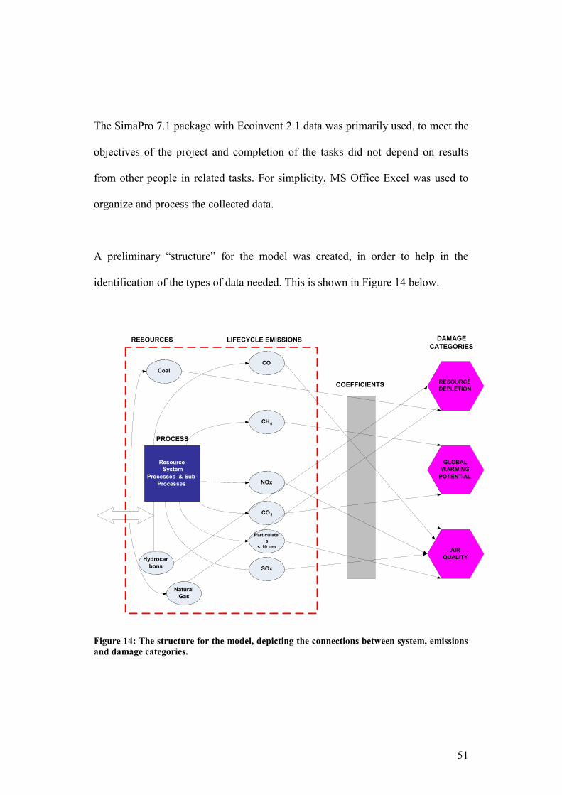
A preliminary “structure” for the model was created, in order to help in the

identification of the types of data needed. This is shown in Figure 14 below.

Figure 14: The structure for the model, depicting the connections between system, emissions

and damage categories.

Resource System

Processes & Sub - Processes

CO Coal

CH 4

Hydrocar bons

NOx

CO 2

Particulate s

< 10 um

Natural Gas

RESOURCE DEPLETION

GLOBAL WARMING

POTENTIAL

AIR QUALITY

SOx

LIFECYCLE EMISSIONS

PROCESS

COEFFICIENTS

DAMAGE CATEGORIES

RESOURCES

52

The interactions between the various emissions and damage categories are

captured in this illustration.

3.2 Environmental Impact Assessment Methods

When attempting to understand the detailed impacts of an urban energy system,

descriptive techniques such as urban metabolism are often not applicable. Even

though the technique gives an excellent overview of the energy flows needed to

sustain a city, it does not allow the researcher or policy-maker to understand the

potential environmental impacts of alternative energy system combinations, such

as, the difference between a district heating system based on biomass sources and

one based on natural gas. The purpose of this section is to illustrate the way in

which Environmental Impact Assessment (EIA) methodologies and Urban Energy

Systems (UES) modelling and optimization techniques can fuse. In order to

achieve that, one step back must be taken to evaluate these methodologies on

UES.

Although a vast number of techniques exist to measure the environmental

“friendliness” of a system, three specific EIAs were chosen for the purposes of

this research:

Material Flow Analysis (MFA)

Ecological Footprints (EF)

Life Cycle Assessment (LCA)

53

These methodologies can be applied to urban energy systems individually or in

combination, in order to indicate what is environmentally acceptable for different

technologies and scenarios.

Ultimately, the aim is to give a recommendation for the design of specific urban

energy system configuration, one that is not economics-oriented, but rather places

an emphasis on environmental impact. In the following sections, one hopes to

highlight some of the practical issues associated with these methods, such as the

types of data required, the feasibility of obtaining this information, the ease of

applying the method, and the technique’s general relevance to the study of urban

energy systems.

3.3 Material Flow Analysis

Material Flow Analysis (MFA) is defined by the holistic analysis of the inputs and

outputs of process sequences, including material extraction or harvest, chemical

transformation, manufacturing, consumption, recycling and disposal of materials.

This method relies upon accounts, measured in physical units (typically tonnes)

that quantify the throughput of such processes. Chemical substances, for example

carbon or carbon dioxide, can be accounted for in this way, as well as natural and

technical compounds, such as coal and wood. MFA carries a clear resemblance to

financial accounting and to traditional economic principles. Despite the fact that

there are small differences in approach based on the research questions being

tackled, the concepts of an industrial metabolism and mass balancing (i.e.

54

ensuring that the net mass in and out of a system is zero) become a common

foundation for MFA studies.

Policy-makers are becoming more and more familiar with the benefits of MFA

and related techniques in their decision-making processes. All of these methods

contribute information to the “know-how” of industrial and urban metabolisms.

The ideal set-up of a sustainable industrial and urban system is given by

consistent and minimized physical exchanges between the environment and

human society, with the internal material cycles being driven by renewable energy

flows (Richards et al., 1994). Having a more sustainable approach to the urban

and industrial metabolism is the desired objective of current governments

worldwide, which has led to the identification of different ways to achieve this

target.

3.3.1 MFA re-named

There are several different “flavours” of material flow analysis and, while the

underlying principles are similar, the focus of the study varies as described below.

Substance Flow Analysis (SFA) Studies of the material flow of a specific

substance are typically known as substance flow analyses. The substance of

interest is often an environmental pollutant like lead, or, in the case of fossil-

fuelled energy systems, carbon dioxide. Accounting for carbon dioxide and other

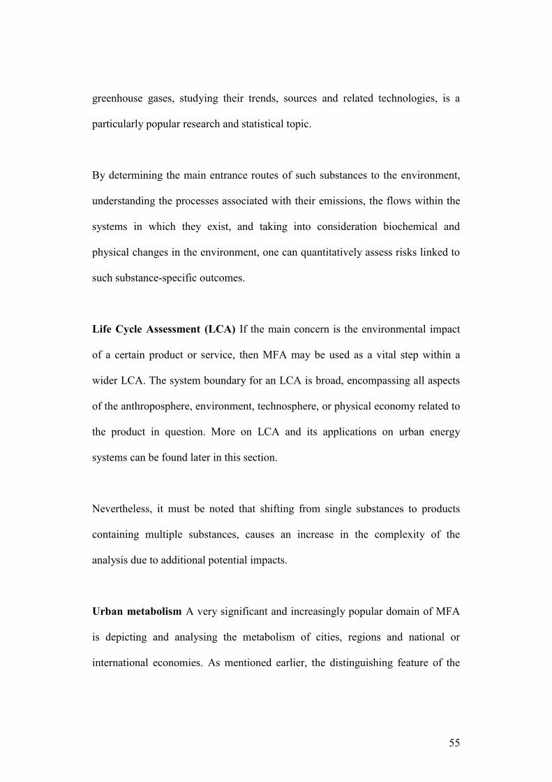
55

greenhouse gases, studying their trends, sources and related technologies, is a

particularly popular research and statistical topic.

By determining the main entrance routes of such substances to the environment,

understanding the processes associated with their emissions, the flows within the

systems in which they exist, and taking into consideration biochemical and

physical changes in the environment, one can quantitatively assess risks linked to

such substance-specific outcomes.

Life Cycle Assessment (LCA) If the main concern is the environmental impact

of a certain product or service, then MFA may be used as a vital step within a

wider LCA. The system boundary for an LCA is broad, encompassing all aspects

of the anthroposphere, environment, technosphere, or physical economy related to

the product in question. More on LCA and its applications on urban energy

systems can be found later in this section.

Nevertheless, it must be noted that shifting from single substances to products

containing multiple substances, causes an increase in the complexity of the

analysis due to additional potential impacts.

Urban metabolism A very significant and increasingly popular domain of MFA

is depicting and analysing the metabolism of cities, regions and national or

international economies. As mentioned earlier, the distinguishing feature of the

56

urban metabolism approach is its use of a system boundary of direct relevance to

a city (rather than a discrete process as in MFA). This type of study is becoming

an essential tool for the evaluation of the sustainability status and trends within

cities.

To achieve these goals, the strategies of “detoxification” and “dematerialization”

of the industrial and urban metabolism are typically adopted. The former refers

primarily to pollution reduction, wherein steps are taken to mitigate the releases of

particular substances to the environment. These have been primarily controlled

using governmental regulations banning certain substances, and additionally by

introducing cleaner technologies. Solutions are typically provided to address the

needs of specific regions and relatively short-term periods (i.e. years). However,

in the case of climate change and greenhouse gas emissions, the drive for long-

term and global solutions creates the need to analyse flows of critical substances,

materials or products, in a systems-wide approach, incorporating cradle-to-grave

techniques.

The second strategy, “dematerialization” relies on the principles of resource

efficiency. By controlling the quantity of primary resources “ingested” by the

urban and industrial systems, the method aims to tackle the problem at its root.

The desire for eco-efficiency includes not only major inputs (e.g. materials,

energy, water) but, at the same time, takes into consideration major outputs to the

57

environment (e.g. emissions to air, water, waste) and associates them with the

products or services produced (EEA, 1999; OECD, 1998).

MFA highlights the importance of acquiring data about industrial and urban

processes. These data collection systems help researchers evaluate the balance of

anthropogenic and natural flows in the economy and environment, but also help

policy-makers to demonstrate the cost efficiency and effectiveness of their

policies. Consequently, a recent review study (Bringezu, 2000) concluded that the

results and findings of MFA-related studies have been used and currently are used

in environmental protection policies:

to support public debate on goals and targets, particularly with respect to

resource and eco-efficiency matters, and the meshing of environmental

and economic policies;

to compile economy-wide material flow accounts for use in official

statistics databases; and

to progress monitoring through the derivation of sustainability indicators.

3.4 Ecological Footprinting

In the case of energy systems, a key consideration is the linkage between the

emissions of carbon dioxide from fossil fuel combustion and its absorption by the

biosphere. In other words, how much land is needed to soak up energy-reated

greenhouse gas emissions? Although this narrow perspective of the ecological

58

footprint of energy systems is strongly critiqued in Ayres and Ayres (2002),

calculations such as the example below, are common (e.g. Barrett et al. 2002).

3.4.1 Calculating the ecological footprint of an energy system

The steps involved in calculating the ecological footprint of an energy system, or

at least the footprint associated with the greenhouse gas emissions are:

1. Calculate the greenhouse gas emissions associated with fossil fuel

combustion. Fossil fuels emit different amounts of carbon dioxide for the

same energy value. Reference tables, such as Table 1, provide these

conversion factors though one must be careful to ensure comparisons are

made on a like-for-like basis. Life cycle analyses of fuel production for

example can change the final emissions level by 30 to 50 per cent (Barrett

et al., 2002).

2. Calculate the land equivalent needed to absorb the emissions. Assuming

that 1GWh of natural gas was burnt, 184 tonnes of CO2 would need to be

absorbed. This number is then converted into the amount of land required

to absorb the CO2, using reference tables to find that 5.2 tonnes of CO2 is

absorbed by 1 hectare of forest: 184/5.2 Since the ecological

footprint works on the concept of a globally average hectare of land, a

further conversion factor must be used to express the relative productivity

of the land type in question to the world average. In this case, it is assumed

that forest is 1.78 times more productive than the global average hectare

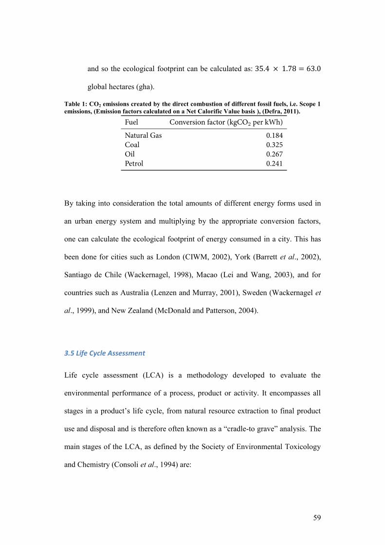
59

and so the ecological footprint can be calculated as:

global hectares (gha).

Table 1: CO2 emissions created by the direct combustion of different fossil fuels, i.e. Scope 1

emissions, (Emission factors calculated on a Net Calorific Value basis ), (Defra, 2011).

By taking into consideration the total amounts of different energy forms used in

an urban energy system and multiplying by the appropriate conversion factors,

one can calculate the ecological footprint of energy consumed in a city. This has

been done for cities such as London (CIWM, 2002), York (Barrett et al., 2002),

Santiago de Chile (Wackernagel, 1998), Macao (Lei and Wang, 2003), and for

countries such as Australia (Lenzen and Murray, 2001), Sweden (Wackernagel et

al., 1999), and New Zealand (McDonald and Patterson, 2004).

3.5 Life Cycle Assessment

Life cycle assessment (LCA) is a methodology developed to evaluate the

environmental performance of a process, product or activity. It encompasses all

stages in a product’s life cycle, from natural resource extraction to final product

use and disposal and is therefore often known as a “cradle-to grave” analysis. The

main stages of the LCA, as defined by the Society of Environmental Toxicology

and Chemistry (Consoli et al., 1994) are:

60

1. Define the goal and scope of the analysis, including the system

boundaries;

2. Compile an inventory of materials and energy use and of emissions and

solid waste, known collectively as “burdens”, associated with the product

or service;

3. Assess the impact of the burdens, with the following steps:

Classification, in which the burdens are aggregated into a smaller

number of environmental impacts;

Characterization, where the potential environmental impacts are

quantified;

Valuation, by which the environmental impacts are reduced to a single

measure of environmental performance;

4. Identify steps to reduce the product’s environmental impacts.

One of the more recently developed methods of life cycle analysis is the Eco-

Indicator 99 Methodology published by PRé Consultants (2001). It has been used

to calculate the environmental impact of a large number of commonly used

materials and processes. The technique attempts to model the potential damages

of a product or service in three damage categories or “endpoints”. These are:

61

Human health – All human beings, in present and future, should be free

from environmentally transmitted illnesses, disabilities or premature

deaths;

Ecosystem quality – Non-human species should not suffer from disruptive

changes of their populations and geographical distribution;

Resources – The nature’s supply of non-living goods, which are essential

to human society, should be available also for future generations.

Four steps are taken to arrive at a value for a particular process (Pre Consultants,

2001) and the method is summarized graphically in Figure 15.

1. The Resource, Land-use and Fate Analysis step, in which the fate of

emissions and the extraction of resources is analysed based on emissions

inventories and feedstock requirements.

2. The Exposure and Effect Analysis step, to determine how much of a

substance released into the environment is actually taken in by living life

forms, such as plants, animals and humans. The effect that resource

extraction has on future generations is also analysed at this stage. The

result is the classification of the impacts according to twelve indicators

such as climate change, ozone layer depletion, acidification and eco-

toxicity.

62

3. The Damage Analysis step quantifies the impact of each category by using

a damage factor and the twelve indicators are then aggregated to form the

main three damage categories mentioned earlier.

4. The Normalization and Weighting step, in which a single aggregated Eco-

Indicator 99 value s calculated through normalization and by assigning

scores and relative weighting factors to each impact category. The

assignment of relative importance is a subjective exercise, hence the

methodology provides three different “perspectives” based upon the

principles of the cultural theory of risk.

63

Figure 15: The Eco-Indicator 99 methodology (Pre Consultants, 2001). SPM = suspended particulate matter, VOC = volatile organic compoun, PAH =

polycyclic aromatic hydrocarbons, HCFC = hydrofluorocarbons.

64

3.5.1 Cultural theory of risk and LCA

The cultural theory of risk (see Thompson et al., 1990) is based on the type of

relations that people have within a group and how an individual’s life has been

moulded by external events, otherwise known as their “grid”. The assumption is

that the position of each individual in this group-grid setup has a large influence

on the value system of individuals and their groups. Hence, these value systems

are used frequently to tackle the problem of modelling subjectivity. The five most

important archetypes that have been identified to generally explain people’s

attitudes are:

1. Individualists, who are relatively free of control by others, yet are often

engaged in controlling others.

2. Egalitarians, who portray no character differentiation, and relations

between group members tend to be ambiguous, causing conflicts.

3. Hierarchists, who are both controlling others, but are also subject to

control by them, bringing a sense of stability to the group.

4. Fatalists, who act alone, lack opinion and are typically controlled by

others.

5. Autonomists, who are usually the smallest group that manages to escape

any manipulative forces from the rest and think completely independently.

The representatives of the first three archetypes are often the most useful in

decision-making, since the have such different opinions between them, whereas

the last two categories represent a smaller range of perspectives.

65

Based on these three personality profiles, Hofstetter (1998) stated that three

versions of an LCA could be produced:

1. The individualist version, where only proven cause-effect relations are

included and short-term perspectives are chosen. For example, in human

health issues, age-weighting is used, due to the individualist’s typically

higher proportion of ages 20-40.

2. The hierarchical version, where facts from recognized scientific and

political bodies are included. A classic example is the accordance with the

IPCC climate change guidelines

3. The egalitarian version, where the largest amount of data is included, with

little omissions and long-term perspectives, since this version is of a

precautionary nature and does not ignore possible future problems.

Consequently, following the completion of an LCA, three possible scores can be

obtained, depending on the cultural theory perspective. The hierarchical version is

usually the default method since its ideology is most common in the scientific

community and in political organizations. The other two methods can provide

basis for sensitivity analyses if desirable. Therefore, the final weighting is heavily

determined by the basic value system a person is using and the concepts of

cultural theory of risk play a large role in its derivation.

The Eco-Indicator 99 Methodology is considered advantageous over other

techniques due to its systematic ideology which produces a single value that is

66

representative of all the different environmental concerns. Equally important is

the fact that the calculations can be ‘interrupted’ at any stage according to the

particular needs of the impact assessment (Hugo et al. , 2004).

3.6 A hypothetical case study

In order to illustrate the way in which LCA and urban energy systems modelling

can fuse, a hypothetical case study was devised for an area of 980 hectares

(divided into 49 cells with 20 ha area each). The purpose is to show potential

energy technology combinations and reductions in environmental impact achieved

through scenario planning and integrated design.

The model for the hypothetical case study was built using the mixed-integer

programming methodology. It includes various technologies, resources and

products and was run to select the least environmentally harmful combination, by

minimizing one damage category at a time. The model is presented in this section,

primarily by stating the main assumptions and the mathematical formulation. As

the equations are linear and include binary and continuous variables, he problem

is classed as an MILP and can be solved using GAMS/CPLEX.

3.6.1 Model Notation and Formulation

The model is formulated as follows; Definitions of the symbols can be found in

this section.

67

SETS

R = Set of resources, r R

EI r = Set of environmental impacts, ei r EI r

Nr r = Set of non-accumulating resources, nr r Nr r

T = Set of technologies, t T

G t = Set of technologies that import resources, g t G t

P t = Set of technologies that consume resources, p t P t

VARIABLES

Q r, i, i’ = Flow of r from i to i’

P r, i = Production of r in cell i

Τ t, i = Production rate of t in i

A r, i = Accumulation of r in i

CAP = Capital cost per annum

ENV = Environmental impact

Z = Objective function

PARAMETERS

TechCC t = Technology capital cost (k£)

TechCap t = Technology capacity in kW

RCost r = Impact value of each resource

D r, i = Demand of each resource in each cell

TransCC r = Transportation capital cost of r per m

MaxTrans r = Maximum rate of transport for resource r

XC i = X co-ordinate of i

YC i = Y co-ordinate of i

distance i, i’ = Distance from i to i’

68

ConvFct t, r = Rate of r produced per rate of operation of t

BINARY VARIABLES

X r, i, i’ = If network exists for i between i and i’

INTEGER VARIABLES

N t, i = Number of t at i

First, the set of resources included in the model is given by

,...}3Re,2Re,1{Re: sourcesourcesourceRr . Some of the resources are used

as feeds to the technologies (e.g. natural gas), whereas others are also considered

as products (e.g. electricity). Environmental impacts (e.g. global warming

potential) were also seen as exiting “resources” from these technologies, in order

to facilitate the formulation of the model. The resources were further sub-divided

into accumulating (i.e. all waste and environmental impacts) and non-

accumulating.

The set of technologies was given by

,...}3log,2log,1log{: yTechnoyTechnoyTechnoTt .These technologies were

sub-divided into technologies that import resources (e.g. electricity grid) and

those that consume resources (e.g. a natural gas boiler).

69

A resource balance is defined for each cell, denoting resources coming in from

outside the cell, plus those produced locally, minus the demand, minus those

leaving the city and must equal to accumulation:

iriiririr

i

iir AQDPQ ,',,,,

'

',, ir, (3.11)

But accumulation must be zero (unless the resource is an environmental impact or

waste):

0, irA (3.12)

The production rate of resource r, in cell i, is given by:

Pr,i = t t,i *ConvFctt,rt

å (3.13)

Where ConvFctt,r is a conversion factor for a given technology and resource, and

is the production rate of technology t, in cell i, given by:

t t,i £ Nt,i *TechCapt (3.14)

t t,i ³ 0 (3.15)

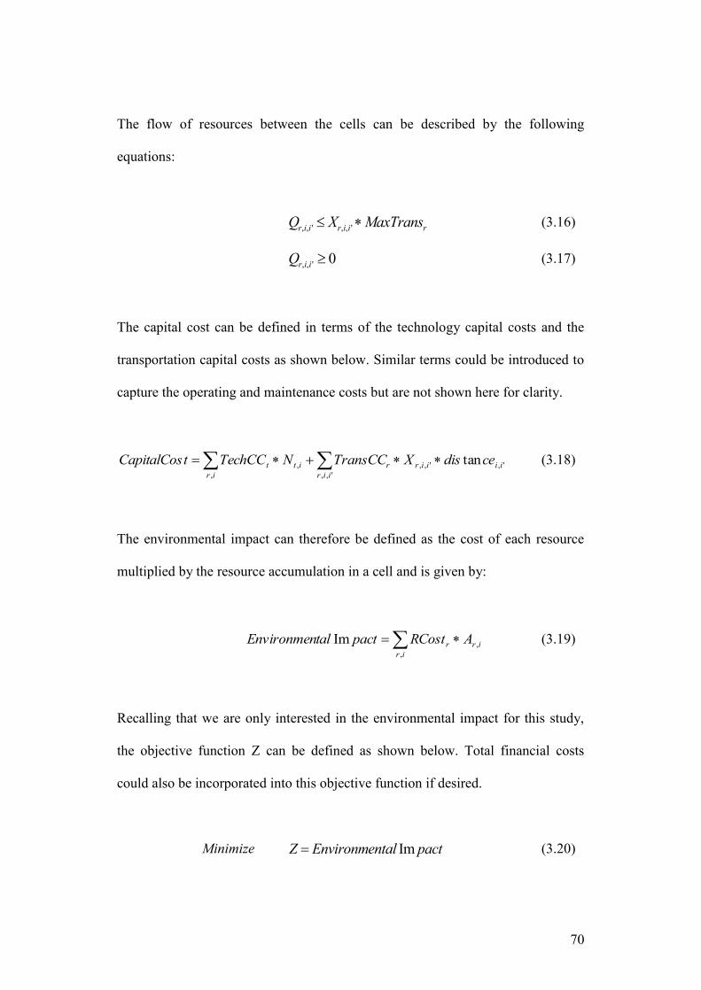
70

The flow of resources between the cells can be described by the following

equations:

Qr,i,i ' £ Xr,i,i ' *MaxTransr (3.16)

Qr,i,i ' ³ 0 (3.17)

The capital cost can be defined in terms of the technology capital costs and the

transportation capital costs as shown below. Similar terms could be introduced to

capture the operating and maintenance costs but are not shown here for clarity.

',',,

, ',,

, tan iiiir

ir iir

ritt cedisXTransCCNTechCCtCapitalCos (3.18)

The environmental impact can therefore be defined as the cost of each resource

multiplied by the resource accumulation in a cell and is given by:

ir

irr ARCostpacttalEnvironmen,

,Im (3.19)

Recalling that we are only interested in the environmental impact for this study,

the objective function Z can be defined as shown below. Total financial costs

could also be incorporated into this objective function if desired.

Minimize Z = Environmental Im pact (3.20)

71

4. RESULTS AND ANALYSIS

4.1 Input data and assumptions

The model begins by specifying the final energy service requirements of the city. The

demands for heat and electricity for this fictional area were estimated on a per-capita

basis to suit the needs of this case study. The algorithm generates random values for

each cell by assuming high demands in the central cells, or otherwise “city-centre”,

and decreasing demands as one proceeds to the outskirts. For each cell, it is assumed

that the demand for heat and electricity can be generated locally otherwise resource

flows take place between cells, as long as a feasible route exists.

A number of energy conversion technologies are then used to convert between raw

input fuels and final energy services. Each technology has a series of parameters

giving their capital cost, operating costs, and resource efficiency, as shown in Table 2.

Table 2: Energy technologies and their approximate capacities based on author estimates. O&M

= operating and maintenance costs.

72

Since minimizing the cost of the energy system configuration is not of primary

interest here, the values shown in the table are estimates. Indeed costs are completely

omitted from the objective function for the present case study so that only

environmental impact affects the results. However, if economic considerations

become of interest at a later stage, the model can be modified, for example using the

constraint method to pursue a multi-objective optimization (e.g. minimizing costs

subject to limits on environmental impact, or minimizing environmental impact

subject to cost constraints). The constraint value can be modified and the model re-run

to generate multiple solutions and thereby explore the interaction between the

economic and environmental objectives.

4.2 Optimization results

The model was run under three different scenarios for minimizing different kinds of

environmental impact, as listed below:

Scenario 1: The objective function was to minimize Global Warming

Potential (GWP);

Scenario 2: The objective function was to minimize Resource Depletion

(RD); and

Scenario 3: The objective function was to minimize Air Quality (AQ).

For each scenario, the results were calculated for all three environmental impact

metrics and these are shown n Table 3:

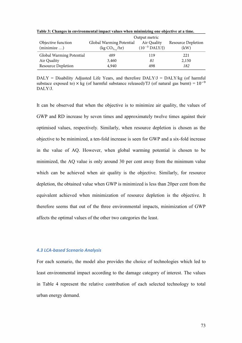
73

Table 3: Changes in environmental impact values when minimizing one objective at a time.

DALY = Disability Adjusted Life Years, and therefore DALY/J = DALY/kg (of harmful

substace exposed to) kg (of harmful substance released)/TJ (of natural gas burnt) = DALY/J.

It can be observed that when the objective is to minimize air quality, the values of

GWP and RD increase by seven times and approximately twelve times against their

optimised values, respectively. Similarly, when resource depletion is chosen as the

objective to be minimized, a ten-fold increase is seen for GWP and a six-fold increase

in the value of AQ. However, when global warming potential is chosen to be

minimized, the AQ value is only around 30 per cent away from the minimum value

which can be achieved when air quality is the objective. Similarly, for resource

depletion, the obtained value when GWP is minimized is less than 20per cent from the

equivalent achieved when minimization of resource depletion is the objective. It

therefore seems that out of the three environmental impacts, minimization of GWP

affects the optimal values of the other two categories the least.

4.3 LCA-based Scenario Analysis

For each scenario, the model also provides the choice of technologies which led to

least environmental impact according to the damage category of interest. The values

in Table 4 represent the relative contribution of each selected technology to total

urban energy demand.

74

Table 4: The model's choice of technologies according to environmental impact. Values indicate

the per cent of total urban energy demand satisfied by a given technology. CHP = combined heat

and power.

To achieve the best results in terms of GWP, the model chose only the biomass

technologies, whereas for RD, it found that a combination of biomass and coal is

better to use as resources. On the other hand, when AQ was the objective, all natural

gas technologies were preferred. The results agree with what was perhaps to be

expected, i.e. biomass technologies tend to have low carbon dioxide emissions which

is considered a significant contributor to global warming. Furthermore, coal is still

abundant in comparison to natural gas reserves and so is biomass, so if resource

depletion minimization is the objective, then natural gas technologies would not

constitute a satisfying solution. Finally, in terms of air quality, all natural gas

technologies were chosen by the model to satisfy the electricity and heat demands,

since very little particulate emissions occur from them.

These results point back to the issue of how different stakeholders might define

“environmental impact”. Each country, government, community and industry will

have its own priorities with respect to which environmental impact is to be

minimized. But as can be seen, the choice of one objective tends to hinder the others

and some view will need to be taken on whether, for example, air quality or global

warming potential is more important.

75

However, one can say that in order to achieve minimum environmental impact,

different system designs need to be considered and incorporated in an urban area. An

optimum combination of energy technologies based on demand and geographical

considerations could possibly satisfy the minimum environmental impact objective.

Of course, the issue becomes even more interesting and complex when cost is

introduced as a more significant component to the objective function. LCA may prove

to overcome the hurdles of other environmental assessment methods by providing a

link between the environmental impacts and the economics of an urban energy

system.

4.4 Selecting EIA methodologies for UES design

Generally, optimization techniques are applied to a problem or case study as a final

step in the process of its analysis and understanding. Optimization results typically

provide quantitative improvement with respect to a system’s initial state. However,

what about taking one step back, and analyzing the system in question in a rather

qualitative manner, to see what can possibly be revealed prior to any quantitative

improvements?

To demonstrate this ideology, a real case study is introduced and put through

environmental impact assessment methodologies. By performing this step, one can

obtain more qualitative information. Specifically, this can show which EIA

methodology (or combination of them) is most relevant and appropriate to the design

of a particular urban energy system and how readily it can be applied.

76

4.5 Scenario Analysis

Three different methods of measuring environmental “friendliness” have been

analyzed and applied to a UK eco-town. These methodologies can be applied to an

urban energy system individually or in combinations to indicate what is

environmentally acceptable for different UES solutions and scenarios.

As mentioned earlier in this report, the case study is a proposed eco-town in England

with an estimated population of 6500 and an overall energy demand of 273

GWh/year, split into 188 GWh of heat demand and 75 GWh of electricity demand.

Five different energy system scenarios were taken into consideration and compared

with respect to the three EIA methodologies: MFA, LCA and EF.

Scenario A: Natural Gas & Electricity Grid (base case)

Scenario B: Natural Gas only

Scenario C: Biomass (Combination of Electricity Grid & Biomass CHP)

Scenario D: Waste-to-Energy (Combination of Anaerobic Digestion,

Electricity Grid & Natural Gas)

Scenario E: Mixed Renewables (Combination of PV Cells, Wind Turbines,

Heat Pumps, Electricity Grid & Natural Gas)

For the purposes of all scenarios, it was assumed that the UK electricity grid

constitutes a mix of 43.5 per cent natural gas, 33 per cent coal, 16.1 per cent nuclear

and the remaining 7.4 per cent representing other fuels (BERR, 2005). For the

biomass scenario (scenario C), it was assumed that 33 per cent of the electricity

demand comes from a biomass CHP, whereas for the waste to energy scenario

77

(scenario D), it was assumed that 20 per cent of the total energy demand can be

produced by the anaerobic digestion of municipal solid waste. For the mixed

renewables scenario (scenario E), it was assumed that 10 per cent of the electricity

demand comes from renewable technologies (i.e. PV cells and wind turbines) and 10

per cent of the heat demand is also produced by renewable technologies (i.e. heat

pumps and solar thermal collectors).

In order to calculate the amount of each fuel needed to run the UK eco-town and thus

obtain values for the material flow analysis, the heat and electricity demands for each

scenario (comprised by the relevant fuel fractions as mentioned in the assumptions)

were divided by the calorific value of each fuel. The calorific values used can be

found in Appendix B.

Table 5 shows the results of the material flow analysis, indicating how much of each

fuel (natural gas, coal and biomass) is required for the smooth operation of each

energy system scenario. All materials are reported in tonnes and give an idea of how

sustainable (or not) each technology is. The major component of each scenario

involves natural gas, with the base case (scenario A) and the mixed renewables option

(scenario E) requiring the largest amounts of coal. Even though the biomass option

(scenario C) requires lower amounts of coal and natural gas, an environmental impact

can be associated with the introduction of just over a million tonnes of wood chips to

fulfil the end-use energy demand of this eco-town.

78

Table 5: Material needed to run the UK eco-town based on five different scenarios.

For the purposes of the life cycle analysis, the total flows of each resource required to

meet the energy demands of the UK eco-town were further multiplied by a

greenhouse gas emission factor. In this manner, the flows were converted to

environmental impact, i.e. quantifying the total greenhouse gases emitted per person.

Based on the results of section 4.1, it has been concluded that out of the three

environmental impacts, namely, air quality, resource depletion and global warming

potential (GWP), the minimization of GWP affects the optimal values of the

remaining two categories the least. GWP is the factor with the greatest impact on a

system and therefore the LCA is conducted on a greenhouse gas (GHG) emissions

basis in this case. Subsequently, the energy systems were compared with respect to

their GHG emissions per capita as shown in Figure 16. It appears at the waste-to-

energy option (scenario D) achieves the lowest GHG emissions per year, whereas the

base case, i.e., using the combination of natural gas for heating purposes and the grid

for electricity demands seems to score the highest.

79

An ecological footprint analysis (measuring how much area of biologically productive

land and water an individual, population or activity requires to produce all the

resources it consumes and to absorb the waste it generates, using prevailing

technology and resource management practices - measured in global hectares) was

also performed. For all five scenarios it was assumed that 150 hectares of productive

land are required to produce 1 GWh of electricity and 65 hectares of productive land

are required to produce 1 GWh from gas for heating purposes. Additionally, it was

assumed that 15 tonnes of biomass are required per hectare for the biomass scenario

(scenario C), as well as 400 tonnes of municipal solid waste per hectare for the waste

to energy scenario (scenario D). For the mixed renewables scenario (scenario E), it

was assumed that 24 hectares of productive land are required to produce 1 GWh from

PV cells, whereas 6 hectares of productive land are required for producing 1 GWh

from a wind turbine. A zero emission factor was assumed for producing heat from

renewable energy technologies. By multiplying these factors with the energy demands

accordingly, the ecological footprint for each scenario can be obtained.

Since the system under study is an energy system, the primary environmental impact

is the greenhouse gas emissions and therefore, the comparison of energy systems

based on ecological footprint follows closely the pattern of the LCA study. However,

the lowest ecological footprint is achieved by scenario B this time, the natural gas

only set-up.

80

Figure 16: The relative environmental impact of urban energy systems of a UK eco-town based

on greenhouse gas emissions per capita (LCA) and ecological footprint per capita.

Following the UK eco-town case study, it was decided to apply the same techniques

to a larger, more complex energy system, like the one of the city of Toronto, Canada.

Toronto is home to 2.6 million inhabitants and has an energy demand of 72,535 GWh

per year. This overall energy demand is sub-divided to 29,878 GWh of electricity

demand and 42,657 GWh of heat demand.

81

Figure 17: Location of Toronto and its census metropolitan area in the province of Ontario

(Wikipedia, 2012).

The same assumptions were used for the Toronto case study as for the UK eco-town

case study in the majority of the model. The only difference was the composition of

the electricity grid. The Canadian grid contains a mix of 6.6 per cent natural gas, 16.6

per cent coal, 15.5 per cent nuclear and the remaining 61.3 per cent other sources such

as hydroelectricity.

The five different energy scenarios were re-applied and Table 6 shows the material

flow analysis for the city of Toronto, indicating how much of each fuel (natural gas,

coal and biomass) is required for the smooth operation of each energy system

scenario. All materials are reported in tonnes again and give an idea of how

sustainable (or not) each technology is. The major component of each scenario

involves natural gas, with the base case (scenario A) and the mixed renewables option

82

(scenario E) requiring the largest amounts of coal. Even though the biomass option

(scenario C) requires lower amounts of coal, an environmental impact can be

associated with the introduction of more than 500 million tonnes of wood chips to

fulfil the end-use energy demand of this eco-town.

Table 6: Material needed to run the city of Toronto based on five different scenarios.

Fuel Consumption (tonnes/year)

Scenarios Natural Gas Coal Biomass

A Natural Gas & Electricity

Grid (Base Case)

8,110,000,000 3,570,000,000 0

B Natural Gas only 13,800,000,000 0 0

C Biomass (Combination of

Electricity Grid & Biomass

CHP)

8,110,000,000 2,380,000,000 528,000,000

D Waste to Energy

(Combination of Anaerobic

Digestion, Electricity Grid &

Natural Gas)

6,490,000,000 2,860,000,000 0

E Mixed Renewables

(Combination of PV Cells,

Wind Turbines, Heat Pumps,

Electricity Grid & Natural

Gas)

8,070,000,000 3,560,000,000 0

The MFA was followed by an LCA in total greenhouse gas emissions and an

ecological footprint analysis.

83

Figure 18: Total Greenhouse gas emissions for the city of Toronto

The energy systems scenarios were compared with respect to their GHG emissions

per capita as shown in Figure 18. It appears that the only natural gas option (scenario

B) achieves the lowest GHG emissions per year, whereas the base case, i.e., using the

combination of natural gas for heating purposes and the grid for electricity demands

seems to score the highest.

84

Figure 19: The ecological footprint for each energy scenario for the city of Toronto

The comparison of energy systems scenarios for Toronto based on ecological

footprint follows closely the pattern of the LCA study. Again, the lowest ecological

footprint is achieved by scenario B, the natural gas only set-up.

85

5. DISCUSSION

The majority of stakeholders concerned argue that using a single environmental

impact assessment methodology to evaluate the sustainability of cities is informative

to the decision-makers involved. Nevertheless, the mode in which these techniques

are currently applied is helpful to specific urban issues and does not really provide an

integrated and insightful measure of urban sustainability as a whole. The dynamic

relationship between the society, the economy and the environment affects a city’s

sustainability to a great extent. The combination of environmental impact assessment

methodologies used in this study presents matters from an energy systems point of

view and facilitates the choice and interpretation of the outcomes. The more these

techniques are combined, e.g. MFA, LCA and EF, the more they help to give a more

specific idea of a system’s performance, while enhancing the output from existing

studies.

The initial objectives that were set for the successful completion of this project have

been satisfied in their majority to the best possible outcome, given the timeframe. A

mathematical model for a hypothetical urban energy system was formulated, which

included various energy technologies, resources and products. The model was run to

select the least environmentally harmful combination of energy technologies, by

minimizing one damage category at a time. Damage categories included global

warming potential, resource depletion and air quality. Additionally, focus was given

on environmental impact assessment methodologies such as material flow analysis,

life cycle assessment and ecological footprint. These methods were applied on a UK

86

eco-town and on the city of Toronto to provide further insight to urban energy

systems. Taking the above into consideration, one can say that the original aims have

been satisfied.

The broader context of the results and outcomes, the strengths or limitations of the

employed approaches, are discussed on an individual basis in the following sub-

sections:

5.1 Life cycle assessment

Many researchers recognize the benefits of LCA as a tool to analyze commensurable

features of quantifiable systems. Nevertheless, not all factors can be brought down to

a single number and used in a model. The need for solid boundaries makes the

accounting of changes within a system, difficult. Furthermore, the availability and

accuracy of the data can also add to inaccuracy (e.g. data may be based on averages,

samples may not be representative or certain results may be outdated). In the case of

LCA applied to energy technologies, one can rename the process to dynamic life

cycle assessment. For example, the growing nature of a power grid must be taken into

consideration, since a specific type of energy technology may emit more carbon

dioxide over its lifetime, than it mitigates. All energy technologies that are trying to

give a solution to the challenge of simultaneously satisfying energy demands, while

reducing carbon emissions, are responsible for some greenhouse gas emissions during

their construction. As these energy technologies expand rapidly, it is essential to

provide policy-makers with standardized information in order to achieve climate

change mitigation.

87

5.2 SimaPro software

SimaPro software was used to obtain LCA data for the initial stages of this research

project. The software brings together inventory data from a wide range of industrial

and economic sectors. Since the inventories are process-based, a user does not need to

determine emissions data for basic inputs, such as electricity use, but instead can use

already available information to simplify an analysis. The already integrated Eco-

Indicator 99 impact assessment tool provides the additional correlation between

inventory data and environmental impacts. Even though this software is applicable to

any process and it is relatively transparent, it can also be characterized as expensive,

labor-intensive and perhaps, containing certain inconsistencies between the different

modules containing the process-based inventory data.

5.3 Material flow analysis

Despite its undisputable usefulness, certain shortcomings and limits can be identidied

for the standard MFA method. Usually large material flows take dominance over all

indicators and affect the interpretation of aggregated results. If only one material

category dominates the MFA, it can lead to biased results by ignoring other material

groups or economic sectors. Ideally MFA should be carried out at a level that

disaggegates economic sectors or material groups. In terms of environmental impacts,

by concluding that the reduction of resource use is necessary, it does not mean that it

is the only precondition for achieving environmental sustainability. The question

would still remain as to which flow has to be reduced to reach a sustainable resource

throughput. Additionally, small material flows, which might not be taken into

account, can potentially have large environmental impacts. An internationally

standardized procedure for considering qualitative changes in the quantitative nature

88

of MFA is at the moment missing. Finally, it would be very beneficial if MFA studies

did not only focus on the presentation of material balances, but to further reflect on

likely policy-related uses of results.

5.4 Urban metabolism

The concept of urban metabolism is a multi-disciplinary way of characterising the

functions within an urban area. Each interpretation has something to offer; MFAs and

urban ecology analyses contribute knowledge that can feed into social and

environmental policy for urban areas. By portraying an urban area as an ecological

system with its own metabolism, it becomes easier to pinpoint the impact of human

activity on the natural environment. Additionally, interpretations of an urban

metabolism can be made from an ecological economics point of view, calling

attention to the environmental and social resources needed to maintain economic

growth. Despite the cross-disciplinary appeal that urban metabolism has, there does

not seem to be enough interdisciplinary engagement in such studies. Undoubtedly, it

would be beneficial to work across disciplines (i.e. integrate industrial and urban

ecology processes with social and political factors), in order to offer the possibility of

new insights, thus increasing the importance of a wealthy and quickly evolving field

of research on the metabolisms of urban areas.

5.5 Ecological Footprints

Generally, the obvious benefit of ecological footprint analysis is its simplicity, since it

becomes a type of indicator that anyone can comprehend. As Wackernagel and Rees

(1996: 230) reasonably observe, “individuals can contrast their personal footprints

with their ecological ‘fair Earthshares’, national footprints can be compared to

89

domestic territories, and the aggregate human footprint can be compared to the

productive capacity of the entire planet.” The resulting concept of “ecological deficit”,

further gives an idea of what a nation’s policy target should be. However, given that

footprint analysis is not dynamic modelling and lacks predictive capability, many

have hinted that this concept is too simplistic. Both nature and the economy are

dynamic systems and it is true that this model does not take full account of the

sustainability story. For example, only the energy consumption is taken into

consideration which confirms the presence of underestimates of the actual ecosystem

appropriations. This means that when the holistic picture of consumption processes is

included in the analyses, the resulting ecological footprints will be much larger than

the current values.

The ecological footprint still forms a significant contribution though. It remains an

estimate of how much energy consumption needs to be reduced, technology needs to

be improved and behaviour needs to be changed to achieve sustainability. The above

limitations do not really detract from the fundamental message of ecological footprint

analysis. As Wackernagel and Rees (1996: 232) further note, “Whatever the

distribution of power or wealth, society will ultimately have to deal with the growing

global ecological debt”.

5.6 Simplistic Approach

As witnessed through the course of this work, biophysical models require an extensive

amount of very specific data in order to portray accurately the flows of the system

under study. Yet, for the sake of simplicity, the standard values available were used.

90

As a result, the analyses were subject to an amount of assumptions and

simplifications, and the overall assessment is also accompanied by uncertainties.

Thus, the approaches could be characterised as reductionistic or simplistic, but one

can say that this is the point of these environmental impact assessment methodologies.

The tools used in assessing an urban energy system, still decreased and integrated the

numerous issues affecting progress towards mitigating an environmental impact to a

smaller set of numbers. The latter is an important tool to policy makers as large

volumes of statistics can be summarised into a comprehensive manner accessible to

non-experts as well.

5.7 “Which EIA methodology (or combination of methodologies) is most relevant and appropriate to the design of a particular UES and how easily can it be applied”?

By applying a combination of the LCA, MFA and ecological footprint methodologies,

a more thorough insight is provided to the dynamic and multi-faceted nature of urban

energy systems. It is not easy to decide which single metric is most important over

others; that is the task of policy-makers and key stakeholders worldwide. Yet, while

there is little doubt that global warming is still a main concern for cities everywhere,

the environmental impact assessment methods presented in this research illustrate

how a range of impacts on health, resource scarcity, and the local and global

environments can be evaluated. It is recommended that all methods used in this

research, both optimization and environmental impact assessment techniques, be

applied to an urban energy system of interest. It is then up to the stakeholders to

prioritise the information revealed, based on social, economic, political and technical

criteria.

91

5.8 What do these results mean to policy-makers?

The approach used for this work might help to identify the key inefficiencies of urban

energy systems configurations which would, in their turn, promote the development of

new technologies or infrastructures. Hopefully, even if this combination of

environmental impact assessment methodologies reveals that the sustainability of a

city is not as high as anticipated, decision-makers will not pose significant resistance

to their adoption because they still provide valuable insights on the system.

By being a fossil-fuel-dependent country, the UK will also face the consequences of

increasing oil prices, since countries and governments are now forced to go after

reserves in places that are harder to access, both geologically and politically. Its turn

towards natural gas is actually leading UK to commit deeper to fossil fuels for its

energy supply, but this resource is also depletable and expensive since it is linked to

oil pricing.

High energy prices can affect a number of sectors within the UK economy. What will

happen with the increase in numbers and popularity of cheap airlines? How will the

tourism be affected? The growth in electricity demand is also of major concern. If

better urban, transportation planning and building design is introduced, then perhaps

power and energy demand in the UK could be reduced or at least maintained constant.

If policy-makers were able to enforce stricter efficiency, conservation and recycling

measures, then maybe the UK would be able to reduce energy consumption. For

example, buildings could be planned and built in a manner to reduce the requirement

of heating and lighting.

92

Perhaps more emphasis should be put on reducing energy use and introducing more

eco-towns with configured set of energy technologies tailored to fit their

specifications. A rational, holistic policy which will consider the various warnings and

devise a preparation strategy would bring enormous benefits to every country’s

energy profile.

The fact remains that urban energy systems still have room for improvement. The

assumption is that a government must provide the increasing energy supply at any

cost, in order to “feed” the unsustainable lifestyle of its population. When changes

start taking place, any population could experience significant upgrades in social,

environmental and economic aspects of its urban life, reminding the reader that

energy does indeed play a pivotal role in a country’s overall wellbeing.

93

6. CONCLUSIONS

Until recently, the optimization of urban energy systems has taken a relatively limited

view of environmental impact, focusing largely on greenhouse has emissions. This

work has sought to widen that perspective, acknowledging the complex characteristics

of urban energy systems that make them stand out with respect to other energy

systems and seeking to provide a better understanding of how such systems function

and interact with respect to various measures of environmental performance. By

evaluating the three different environmental impact assessment methodologies, it was

shown how qualitative and quantitative analyis techniques can be used to provide

additional insight to an urban energy system at various aspects of its functionality.

Having carried out this research, I was able to conclude that:

Cities play a determining role in the evolution of the energy sectors worldwide

due to their large heat and power demands. Consequently, improving the

efficiency of urban energy systems is an increasingly important issue.

Urban energy systems can be seen as eco-systems and all the processes taking

place within them, form an urban metabolism characterized by inputs, outputs,

and accumulation of various materials.

The Synthetic City Toolkit, and particularly the Resource Technology

Network component, formed a solid basis for this research and outcomes from

this research can complement this component of the toolkit.

Having studied the work of researchers in the fields of optimization, urban

metabolism and life cycle assessment methodologies, a gap was identified in

94

the research that combines optimization techniques and environmental impact

assessment methodologies to evaluate urban energy systems, specifically.

Data had to be collected from a variety of databases, and software, and

numerous assumptions had to be made at different stages of the research to

build models both in GAMS and in Excel. In many cases, data was not readily

available and a certain amount of uncertainty can be attributed to values used

to populate the models.

Life cycle assessment and urban metabolism can be classified as different

types of material flow analysis. On the other hand, the ecological footprint can

be seen as a rather different approach to characterize urban energy systems.

Environmental impact assessment methodologies and optimization techniques

can fuse to identify the combination of energy technologies that best meet the

heat and electricity demand requirements of an urban energy system, while

minimizing a specific environmental damage category at a time.

By minimizing global warming potential specifically, the remaining two

damage categories of air quality and resource depletion deviate the least from

their optimal values.

By performing a material flow analysis and a life cycle assessment, and by

calculating the ecological footprint of a UK eco-town and the city of Toronto,

it is proven that different information can be deduced through each

environmental impact assessment methodology and that each of them provides

additional insight to these urban energy systems.

Water withdrawn specifically for the needs of the energy industries present in

the two case studies, can also become a measure of environmental friendliness

95

and sustainability. Indirect material flows, such as water in energy, should not

be neglected when looking at an urban energy system.

The three environmental impact assessment methodologies used are

characterized by both advantages and disadvantages in their ideologies.

However, they were chosen as the most suitable for application in this

research.

In order to get a holistic view of the environmental impacts associated with the

design of a particular urban energy system, it is recommended to apply all

three environmental impact assessment methodologies in combination with

optimization techniques. The information obtained can then be filtered

according to the needs of the stakeholders interested.

Further interpretation of the environmental impact assessment methodologies

in terms of social and economic factors would prove valuable to policy-

makers.

6.1 Recommendations for Future Work

The technical relevance of the outcomes was to provide further insight to

urban energy systems and a combination of approaches, which can, in the

future be applied to other similar cities. Cities in developing countries would

be particularly interesting to look at, since they could potentially integrate the

improved efficiencies inherently, during their expansion.

It would also be beneficial to formally embed the environmental impact

assessment methods into existing urban energy systems tools. By integrating

these concepts into urban modeling tools, a more interdisciplinary perspective

will be adopted.

96

Additionally, it would be useful to ultimately connect the energy flows in an

urban area with other resources, such as waste and food.

If more time had been available to elaborate this study, the optimal values of

the decision variables could be shown on a pixelated grid diagram. A graph

showing the Q values for the hypothetical case study could provide some

interesting information. In this way, information about the location and choice

of technologies and capacities could also be provided.

Furthermore, the results could be shown as spatial distributions in order to

demonstrate the advantage of using optimization methodologies (for spatial

information generation) over the LCA packages (providing aggregated

results).

Multi-objective optimization work to account for economic optimization of the

various scenarios and technology options would give further insight to this

study, thus combining both the financial, as well as the environmental aspect

for decision-makers. Hence, it would be beneficial to include a total cost for

each scenario, if there were no time constraints.

Ideally, the active engagement of the public in collecting data needed for these

studies would facilitate the process majorly. It would be very interesting to

involve the inhabitants of the urban energy systems under investigation in

choosing priorities.

97

7. REFERENCES

Alexandre, A. and De Michelis, N., (1996). Environment and energy: lessons from the

North. Environmental Impact Assessment Review 16, 249-257.

Ayres, R., and Ayres, L., (2002). A Handbook of Industrial Ecology.

Azapagic, A. (1999). Life cycle assessment and its application to process selection,

design and optimisation. Chemical Engineering Journal 73, 1-21.

Azapagic, A. and Clift, R., (1995). Life cycle assessment and linear programming –

environmental optimisation of a product system. Computers & Chemical Engineering.

19(S), S229-S234.

Azapagic, A. and Clift, R., (1999). Allocation of environmental burdens in multiple-

function systems. Journal of Cleaner Production 7, 101-119.

Azapagic, A. and Clift, R., (1999). Life cycle assessment and multiobjective

optimisation. Journal of Cleaner Production 7, 135-143.

Azapagic, A., Pettit, C. and Sinclair, P., (2007). A life cycle methodology for

mapping the flows of pollutants in the urban environment. Journal for Clean

Technologies and Environmental Policy 9, 199-214.

Baccini, P., (1997). A city’s metabolism: Towards the sustainable development of

urban energy systems. Journal of Urban Technology 4(2): 27-39.

Barrett, J., Vallack, H., Jones, A. and Haq, G., (2002). A Material Flow Analysis and

Ecological Footprint of York. Stockholm Environment Institute.

BERR (2005). Electricity (Fuel Mix Disclosure) Regulations.

98

BP and Imperial College, (2006) BP-Imperial College Urban Energy Systems Project:

First Annual Report, Energy Futures Lab (Imperial College London, UK)

Bringezu, S., (2000). Industrial Ecology and Material Flow Analysis. Proceedings of

the International Symposium “Industrial ecology and sustainability”, Troyes, France,

Technical University of Troyes, September 22-25, 1999.

Chartered Institute of Wastes Management (2002). A Resource Flow and Ecological

Footprint Analysis of Greater London. Best Foot Forward, London.

Consoli, F. et al., eds., (1993). Guidelines for life cycle assessment: A “Code of

practice”, SETAC, Brussels and Pensacola.

DEFRA (2011). 2011 Guidelines to Defra/DECC’s GHG conversion factors for

company reporting.

Duvigneaud, P., and Denaeyer-De Smet, S., (1977). L’ecosysteme urbain bruxellois.

Traveaux de la Section Belge du Programme Biologique International, Brussels.

Paris: Edition Duculot.

European Environment Agency (EEA) (1999). Environment in the European Union at

the Turn of the Century, Copenhagen: European Environment Agency.

Girardet, H., (1995). The Gaia Atlas of Cities. Gaia Books Limited, London.

Global Footprint Network, (2007) (09/08/07): Humanity’s footprint 1961-2003.

http://www.footprintnetwork.org/gfn_sub.php?content=global_footprint

Hanya, T., and Ambe, Y., (1976). A study on the metabolism of cities. In Science for

a better environment. Tokyo: HESC, Science Council of Japan.

Hendriks, C., Obernosterer, R., Muller, D., Kytzia, S., Baccini, P., and Brunner, P.

(2002). Material flow analysis: A tool to support environmental policy decision

99

making. Case studies on the city of Vienna and the Swiss lowlands. Local

Environment 5: 311-328.

Hofstetter, P., (1998). Perspectives in Life Cycle Impact Assessment; A Structured

Approach to Combine Models of the Technosphere, Ecosphere and Valuesphere.

Kluwers Academic Publishers. www.wkap.nl/book.htm/07923-8377-X.

Hugo, A., Ciumei, C., Buxton, A. and Pistikopoulos, E., (2004). Environmental

impact minimization through material substitution: a multi-objective optimization

approach. Journal of Green Chemistry 6, 407-417.

Hugo, A., Rutter, P., Pistikopoulos, S., Amorelli, A. and Zoia, G., (2005). Hydrogen

infrastructure strategic planning using multi-objective optimization. International

Journal of Hydrogen Energy 30, 1523-1534.

International Energy Agency, 2004 (25/08/07): World Energy Outlook 2004.

http://www.iea.org//textbase/nppdf/free/2004/weo2004.pdf

International Energy Agency, (2011). World Energy Outlook 2011, IEA, Paris, 2011.

Jaccard, M. K., (2005). Sustainable Fossil Fuels: The Unusual Suspect in the Quest

for Clean and Enduring Energy (Cambridge University Press, Cambridge, UK).

Keristead, J. and Calderon, C., (2012). Capturing spatial effects, technology

interactions, and uncertainty in urban energy and carbon models: Retrofitting

Newcastle as a case-study. Energy Policy 46: 253-267.

Keirstead, J., Samsatli, N., Pantaleo, A. M., Shah, N., (2009). Evaluating integrated

urban biomass strategies for a UK eco-town. In Proceedings of the European Biomass

Conference, Hamburg.

Keirstead, J., Samsatli, N., Shah, N., (2009). SynCity: an integrated tool kit for urban

energy systems modelling. In Proceedings of the 5th

Urban Research Symposium,

Marseille.

100

Keirstead, J., Samsatli, N., Shah, N., Weber, C. and Fisk, D., (2010). The implications

of CHP planning restrictions on the efficiency of urban energy systems. In 23rd

International Conference on Efficiency, Cost, Optimization, Simulation and

Environmental Impact of Energy Systems, Lausanne.

Keirstead, J., Samsatli, N., Pantaleo, A., and Shah, N., (2012a). Evaluating biomass

energy strategies for a UK eco-town with an MILP optimization model. Biomass and

Bioenergy 39: 306-316.

Keirstead, J., Jennings, M., and Sivakumar, A., (2012b). A review of urban energy

system models: Approaches, challenges and opportunities. Renewable and

Sustainable Energy Reviews 16(6): 3847-3866.

Kennedy, C., Cuddihy J., and Engel-Yan, J., (2007). The changing metabolism of

cities. Journal of Industrial Ecology 11(2): 43-59.

Lei, K., and Wang, Z., (2003). The analysis of ecological footprints of Macao I 2001.

Journal of Natural Resources, 2003-02.

Lenzen, M., and Murray, S., (2001). A modified ecological footprint method and its

application to Australia, Ecological Economics 37(2): 229-255.

Liang, H., Long, W. D., Keirstead, J., Samsatli, N., and Shah, N., (2012) Urban

Energy Systems Planning and Chinese Low-Carbon Eco-City Case Study. Advanced

Materials Research, 433-440, 1338-1345.

Liu, P., Pistikopoulos, E. N. and Li, Z., (2009). A multi-objective optimization

approach to polygeneration energy systems design. Preprint submitted to AIChE J,

July 21, 2009.

McDonald, G., and Patterson, M., (2004). Ecological Footprints and

interdependencies of New Zealand regions. Ecological Economics 50(1-2): 49-67.

101

Newcombe, K., Kalina, J., and Aston, A., (1978). The metabolism of a city: The case

of Hong Kong. Ambio 7: 3-15.

Newman, P., (1999). Sustainability and cities: Extending the metabolism model.

Landscape and Urban Planning 44: 219-226.

Odum, H., (1983). Systems Ecology, an Introduction. Wiley-Interscience, New York.

Organization for Economic Cooperation and Development (OECD) (1998). Towards

sustainable development: Environmental Indicators, Paris: OECD.

PRe Consultants, (2001). The Eco-Indicator 99, A damage oriented method for Life

Cycle Impact Assessment, Methodology Report. Third edition, Amersfoort,

Netherlands.

Richards, D., Brade, J., Allenby, R., and Frosch, R. (1994). The greening of industrial

ecosystems: Overview and perspective. The Greening of Industrial Ecosystems,

Washington DC: National Academy Press, pp. 1-22.

Sahely, H. R., Dudding, S., and Kennedy, C., (2003). Estimating the urban

metabolism of Canadian cities: GTA case study. Canadian Journal for Civil

Engineering 30: 468-483.

Schulz, N. B., (2005). Contribution of material and energy flow accounting to urban

ecosystems analysis: case study Singapore, Yokohama: UNU-IAS Working Paper No

136.

Shah, N., Fisk, D., Davies, A., Gann, D., Hernandez, C., Leach, M., Ozaki, R.,

Pistikopoulos, E., Pearson, P., Polak, J., Walton C., Woods, L., Frederiksen, A.,

Frenzel, A., Keirstead, J., Samsatli N., Schulz, N. B., Acha, S., Barklund, E.,

Samaraweera, M. and Villareal, R., (2006). BP – Imperial College Urban Energy

Systems Project: First Annual Report. Imperial College London.

102

Shah, N., Fisk, D., Davies, A., Gann, D., Hernandez, C., Leach, M., Ozaki, R.,

Pistikopoulos, E., Pearson, P., Polak, J., Walton C., Woods, L., Frederiksen, A.,

Frenzel, A., Keirstead, J., Samsatli N., Schulz, N. B., Acha, S., Barklund, E.,

Samaraweera, M. and Villareal, R., (2010). BP – Imperial College Urban Energy

Systems Project: Fifth Annual Report. Imperial College London.

Smil ,V., (2008). Energy in Nature and Society, Massachusetts: The MIT Press, p.

320-324.

Stanhill, G., (1977). A urban agro-ecosystem: the example of nineteenth-century

Paris. Agro-Ecosystems 3: 269-284.

Stefanis, S. K., Livingston, A.G., and Pistikopoulos E.N., (1995). Minimizing the

environmental impact of process plants: A process systems methodology. Computers

& Chemical Engineering. 19(S), S39-S44.

Thomas, R., (2003). Sustainable urban design: an environmental approach. Spon

Press, London.

Thompson, M., Ellis, R., Wildavsky, A., (1990). Cultural Theory. Westview Print

Boulder.

United Nations Department of Economic and Social Affairs, 2006 (25/08/07): World

urbanization prospects: The 2005 revision.

http://www.un.org/esa/population/publications/WUP2005/2005WUPHighlights_Final

_Report.pdf

United Nations Habitat, (2007) (08/09/07): Climate Change Statement by Brian

Williams, UN Commission on Sustainable Development, 15th

Session. New York:

UN-HABITAT.

http://www.unhabitat.org/content.asp?cid=4756&catid=356&typeid=8&subMenuId=

0

103

United Nations World Commission on Environment and Development, 1987

(25/08/07): Our Common Future: The Brundtland report. http://www.un-

documents.net/wced-ocf.htm

Wackernagel, M., and Rees, W., (1996). Urban ecological footprints: why cities

cannot be sustainable and why they are a key to sustainability. Environ Impact Assess

Rev, 16: 223-248.

Wackernagel, M., (1998). The ecological footprint of Santiago de Chile. Local

Environment: The International Journal of Justice and Sustainability, 3(1): 7-25.

Wackernagel, M., Lewan, L., and Borgstromm Hansson, C., (1999). Evaluating the

use of Natural Capital with the Ecological Footprint, Applications in Sweden and

Subregions, Ambio, 28(7): 604.

Wackernagel, M., Onisto, L., Bello, P., Callejas Linares A., Falfan I. S., Garcia, J.,

Guerrero, A. I. and Guerrero, M. G., (1999). National natural capital accounting with

the ecological footprint concept. Ecological Economics, 29: 375-390.

Warren-Rhodes, K., and Koenig, A., (2001). Escalating trends in the urban

metabolism of Hong Kong: 1971-1997. Ambio 30(7): 429-438.

Weber, C., and Shah, N. (2011). Optimization based design of a district energy system

for an eco-town in the United Kingdom. Energy 36(2): 1292-1308.

Wikipedia, 2012 (25/08/12): Wikipedia, The free encyclopaedia: Toronto.

http://en.wikipedia.org/wiki/Toronto

Wolman, A., (1965). The metabolism of cities. Scientific American 213(3): 179-190.

WWF, (2006) (09/08/07): Living Planet Report 2006.

http://assets.panda.org/downloads/living_planet_report.pdf

104

Zucchetto, J., (1975). Energy economic theory and mathematical models for

combining the systems of man and nature. Case study, the urban region of Miami.

Ecological Modelling 1: 241-268.

105

8. APPENDICES

8.1 Appendix A – Input data used in the GAMS model

$TITLE City Layout 49 cells model

OPTION SOLPRINT = OFF ;

OPTION LIMCOL = 0 ;

OPTION LIMROW = 0 ;

$OFFSYMXREF

$OFFSYMLIST

*

* MILP formulation for first city layout model

SCALAR

NCS number of cells

ALPHA /0/

AREA area of each cell in Ha /20/

LEN length of each cell in m /400/

BIGM large number /350/ ;

SETS

row row index /1*7/

col column index /1*7/

i grid square index /1*49/

*

* 7 by 7 square

*

r resources /'gas', 'elec', 'coal', 'biomass',

'heat', 'dist_heat', 'waste_heat', 'ghg', 'aq', 'rd'/

ei(r) environmental impacts /'ghg', 'aq', 'rd'/

nr(r) non accumulating /'gas', 'elec', 'coal', 'biomass', 'heat', 'dist_heat'/

t technologies /'ele_grid', 'ng_grid', 'coal_imp', 'biomass_imp',

'ng_chp', 'ng_boiler', 'coal_chp', 'biomass_chp', 'biomass_boiler',

'heat_ex'/

g(t) technologies that import resources /'ele_grid', 'ng_grid', 'coal_imp'/

p(t) technologies that consume resources

;

p(t) = NOT(g(t)) ;

ALIAS

(i, i1),

(i, i2),

(r, r1);

106

SETS

rci(row,col,i) association between i row and col ;

rci(row,col,i)$(ORD(i) = ORD(col) + (ORD(row)-1)*CARD(col)) = YES ;

NCS = CARD(i) ;

PARAMETERS

TechCC(t) technology capital cost k£

/ele_grid=1000, ng_grid=100, coal_imp=100, biomass_imp=100,

ng_chp=1500, ng_boiler=1, coal_chp=2000, biomass_chp=1700, biomass_boiler=2,

heat_ex=0.2/

TechCap(t) technology capacity in kWth or kWe

/ele_grid=45000, ng_grid=45000, coal_imp=45000, biomass_imp=45000,

ng_chp=45000, ng_boiler=2, coal_chp=45000, biomass_chp=45000,

biomass_boiler=2, heat_ex=2/

RCost (r) cost of each resource

Demand(r, i) demand of each resource in each cell

TransCC (r) transportation capital cost of r per m

/gas=1, elec=1, coal=1, biomass=1, heat=1, dist_heat=200, waste_heat=0, ghg=0,

aq=0, rd=0/

MaxTrans(r) maximum rate of transport for resource r

/gas=1E6, elec=1E6, coal=1E6, biomass=1E6, heat=0, dist_heat=1E6, waste_heat=0,

ghg=0, aq=0, rd=0/

XC (i) x co-ordinate of i

YC (i) y co-ordinate of i

dist (i, i1) distance from i to i1

;

LOOP( (row,col),

LOOP( i$rci(row,col,i),

YC(i) = ORD(row)*LEN ;

XC(i) = ORD(col)*LEN ;

) ;

) ;

TABLE CF (t, r) 'rate of r produced per rate of operation of t'

gas elec coal biomass heat dist_heat waste_heat

ghg aq rd

ele_grid 0 1 0 0 0 0 0 480

7.93E-2 3.68E-2

ng_grid 1 0 0 0 0 0 0 0 0

0

107

coal_imp 0 0 1 0 0 0 0 0 0

0

biomass_imp 0 0 0 1 0 0 0 36

9.36E-3 1.30E-1

ng_chp -2.5 1 0 0 0 1.5 0 261

5.96E-3 1.63E-1

ng_boiler -1.1 0 0 0 1 0 0.1 265

6.58E-3 1.63E-1

coal_chp 0 1 -2.5 0 0 1.5 0 533

5.08E-2 1.19E-2

biomass_chp 0 1 0 -2.5 0 1.5 0 36

8.51E-3 1.63E-2

biomass_boiler 0 0 0 -1.2 1 0 0.2 36

9.36E-3 1.63E-2

heat_ex 0 0 0 0 1 -1 0 0 0

0 ;

*

*

=============================================================

===================

* ghg is g/kWh aq is DALY/TJ RD is MJ surplus/m3

*

=============================================================

===================

*

* to make the environmental metrics per rate of process, need to multiply by the

* amount of resource consumed (gas, coal, etc.)

CF(p,ei) = CF(p,ei)*SUM( r1$(CF(p,r1) < 0), -CF(p,r1) ) ;

* \_ find the resource being consumed by p

Rcost('ghg')=1;

dist(i,i1) = SQRT( SQR(XC(i) - XC(i1)) + SQR(YC(i) - YC(i1)) ) ;

demand('elec','1') = 269206.442117691;

demand('heat','1') = 685352.623462677;

demand('elec','2') = 247891.813755035;

demand('heat','2') = 716360.218524933;

demand('elec','3') = 253473.224401474;

demand('heat','3') = 610171.446800232;

demand('elec','4') = 238388.124465942;

demand('heat','4') = 675722.227096558;

demand('elec','5') = 263804.799318314;

demand('heat','5') = 662404.716014862;

demand('elec','6') = 211943.902492523;

demand('heat','6') = 540780.808925629;

demand('elec','7') = 297771.082639694;

demand('heat','7') = 628012.437820435;

108

demand('elec','8') = 201420.079231262;

demand('heat','8') = 667813.353538513;

demand('elec','9') = 248705.6620121;

demand('heat','9') = 689727.079868317;

demand('elec','10') = 266085.789203644;

demand('heat','10') = 500035.727024078;

demand('elec','11') = 252432.359457016;

demand('heat','11') = 586604.351997375;

demand('elec','12') = 202969.932556152;

demand('heat','12') = 752465.553283691;

demand('elec','13') = 290741.793870926;

demand('heat','13') = 777948.987483978;

demand('elec','14') = 269962.737560272;

demand('heat','14') = 508660.495281219;

demand('elec','15') = 213617.943525314;

demand('heat','15') = 676615.524291992;

demand('elec','16') = 214667.323112488;

demand('heat','16') = 784331.53629303;

demand('elec','17') = 270214.708566666;

demand('heat','17') = 726684.086322784;

demand('elec','18') = 247001.261234283;

demand('heat','18') = 812831.26115799;

demand('elec','19') = 302582.473516464;

demand('heat','19') = 680511.164665222;

demand('elec','20') = 329548.139572144;

demand('heat','20') = 667517.137527466;

demand('elec','21') = 336144.669771194;

demand('heat','21') = 630155.398845673;

demand('elec','22') = 263659.123897552;

demand('heat','22') = 735989.797115326;

demand('elec','23') = 216924.338102341;

demand('heat','23') = 788178.358078003;

demand('elec','24') = 217304.520606995;

demand('heat','24') = 641206.316947937;

demand('elec','25') = 257520.691156387;

demand('heat','25') = 842820.32251358;

demand('elec','26') = 342211.194038391;

demand('heat','26') = 714709.000587463;

demand('elec','27') = 230956.043958664;

demand('heat','27') = 648716.931343079;

demand('elec','28') = 336092.998027802;

demand('heat','28') = 697125.389575958;

demand('elec','29') = 285807.591676712;

demand('heat','29') = 788669.812679291;

demand('elec','30') = 331456.136703491;

demand('heat','30') = 670492.315292358;

demand('elec','31') = 344798.875570297;

demand('heat','31') = 855768.032073975;

demand('elec','32') = 227033.916950226;

demand('heat','32') = 752825.601100922;

109

demand('elec','33') = 279522.577524185;

demand('heat','33') = 631582.100391388;

demand('elec','34') = 241096.755027771;

demand('heat','34') = 600612.750053406;

demand('elec','35') = 218838.957548141;

demand('heat','35') = 673175.692558289;

demand('elec','36') = 244225.614070892;

demand('heat','36') = 513012.163639069;

demand('elec','37') = 262524.291276932;

demand('heat','37') = 790742.366313934;

demand('elec','38') = 226335.441589355;

demand('heat','38') = 669177.360534668;

demand('elec','39') = 306169.307470322;

demand('heat','39') = 630867.280960083;

demand('elec','40') = 291948.606967926;

demand('heat','40') = 663706.195354462;

demand('elec','41') = 311327.625513077;

demand('heat','41') = 760413.916110992;

demand('elec','42') = 225718.33896637;

demand('heat','42') = 705215.077400208;

demand('elec','43') = 298914.192914963;

demand('heat','43') = 696035.79044342;

demand('elec','44') = 294202.163219452;

demand('heat','44') = 623038.189411163;

demand('elec','45') = 263853.722810745;

demand('heat','45') = 744313.180446625;

demand('elec','46') = 213885.339736938;

demand('heat','46') = 507051.706314087;

demand('elec','47') = 236979.13146019;

demand('heat','47') = 647514.839172363;

demand('elec','48') = 247454.300403595;

demand('heat','48') = 705623.013973236;

demand('elec','49') = 256179.975748062;

demand('heat','49') = 529984.714984894;

*demand(r,i) = demand(r,i)/1000 ;

DISPLAY

Dist, CF, techcap ;

VARIABLES

QR (r, i, i1) flow of r from i to i1

PR (r, i) production of r in cell i

PT (t, i) production rate of t in i

AC (r, i) accumulation of r in i

CAP the capital cost

ENV environmental impact

Z the objective function ;

110

POSITIVE VARIABLES

QR, PT, AC, CAP;

BINARY VARIABLES

XQ (r, i, i1) if network exists for i between i and i1 ;

INTEGER VARIABLES

NT (t, i) number of t at i ;

NT.UP('heat_ex',i) = 1000000 ;

NT.UP('ng_boiler',i) = 1000000 ;

NT.UP('biomass_boiler',i) = 1000000 ;

XQ.FX(r,i,i) = 0 ;

EQUATIONS

ResBal resource balance

AcCon AC must be zero unless a waste or environmental impact

ProdRate production rate of resource r in i

TechRate technology rate cap

FlowRate resource flow between i and i1

CapDef definition of capital cost

EnvDef definition of capital cost

ObjDef definition of objective function ;

* Resource balance for each cell

ResBal(r,i).. SUM( i1, QR(r,i1,i) ) + PR(r,i)

- demand(r,i)/3600 - SUM( i1, QR(r,i,i1) ) =E= AC(r,i) ;

AcCon(nr,i).. AC(nr,i) =L= 0 ;

* production of resource r in cell i

ProdRate(r,i).. PR(r,i) =E= SUM( t, CF(t,r)*PT(t,i) ) ;

* production rate of technology t in cell i

TechRate(t,i).. PT(t,i) =L= NT(t,i)*TechCap(t) ;

* flow of resources between cells

FlowRate(r,i,i1).. QR(r,i,i1) =L= XQ(r,i,i1)*MaxTrans(r) ;

* capital cost

CapDef.. CAP =E= SUM( (t,i), TechCC(t)*NT(t,i) ) +

SUM( (r,i,i1), TransCC(r)*XQ(r,i,i1)*dist(i,i1) +

0.00001*QR(r,i,i1));

* environmental impact

EnvDef.. ENV =E= SUM( (r,i), Rcost(r)*AC(r,i) ) ;

* objective function

111

ObjDef.. Z =E= CAP/1000 + ENV ;

OPTION ITERLIM = 200000 ;

*OPTION OPTCR = 0.01 ;

MODEL Zeus / ALL / ;

SOLVE Zeus USING MIP MINIMIZING Z ;

DISPLAY Demand, NT.L, PT.L, PR.L, AC.L ;

DISPLAY XQ.L, QR.L ;

DISPLAY CAP.L, ENV.L, Z.L ;

Table 7: Heat and electricity demands per cell number

Type of Demand (cell number) Value

demand('elec','01') 269206.4

demand('elec','02') 247891.8

demand('elec','03') 253473.2

demand('elec','04') 238388.1

demand('elec','05') 263804.8

demand('elec','06') 211943.9

demand('elec','07') 297771.1

demand('elec','08') 201420.1

demand('elec','09') 248705.7

demand('elec','10') 266085.8

demand('elec','11') 252432.4

demand('elec','12') 202969.9

demand('elec','13') 290741.8

demand('elec','14') 269962.7

demand('elec','15') 213617.9

demand('elec','16') 214667.3

demand('elec','17') 270214.7

demand('elec','18') 247001.3

demand('elec','19') 302582.5

demand('elec','20') 329548.1

demand('elec','21') 336144.7

demand('elec','22') 263659.1

demand('elec','23') 216924.3

demand('elec','24') 217304.5

demand('elec','25') 257520.7

demand('elec','26') 342211.2

demand('elec','27') 230956

demand('elec','28') 336093

demand('elec','29') 285807.6

demand('elec','30') 331456.1

112

demand('elec','31') 344798.9

demand('elec','32') 227033.9

demand('elec','33') 279522.6

demand('elec','34') 241096.8

demand('elec','35') 218839

demand('elec','36') 244225.6

demand('elec','37') 262524.3

demand('elec','38') 226335.4

demand('elec','39') 306169.3

demand('elec','40') 291948.6

demand('elec','41') 311327.6

demand('elec','42') 225718.3

demand('elec','43') 298914.2

demand('elec','44') 294202.2

demand('elec','45') 263853.7

demand('elec','46') 213885.3

demand('elec','47') 236979.1

demand('elec','48') 247454.3

demand('elec','49') 256180

demand('heat','01') 685352.6

demand('heat','02') 716360.2

demand('heat','03') 610171.4

demand('heat','04') 675722.2

demand('heat','05') 662404.7

demand('heat','06') 540780.8

demand('heat','07') 628012.4

demand('heat','08') 667813.4

demand('heat','09') 689727.1

demand('heat','10') 500035.7

demand('heat','11') 586604.4

demand('heat','12') 752465.6

demand('heat','13') 777949

demand('heat','14') 508660.5

demand('heat','15') 676615.5

demand('heat','16') 784331.5

demand('heat','17') 726684.1

demand('heat','18') 812831.3

demand('heat','19') 680511.2

demand('heat','20') 667517.1

demand('heat','21') 630155.4

demand('heat','22') 735989.8

demand('heat','23') 788178.4

demand('heat','24') 641206.3

demand('heat','25') 842820.3

demand('heat','26') 714709

demand('heat','27') 648716.9

113

demand('heat','28') 697125.4

demand('heat','29') 788669.8

demand('heat','30') 670492.3

demand('heat','31') 855768

demand('heat','32') 752825.6

demand('heat','33') 631582.1

demand('heat','34') 600612.8

demand('heat','35') 673175.7

demand('heat','36') 513012.2

demand('heat','37') 790742.4

demand('heat','38') 669177.4

demand('heat','39') 630867.3

demand('heat','40') 663706.2

demand('heat','41') 760413.9

demand('heat','42') 705215.1

demand('heat','43') 696035.8

demand('heat','44') 623038.2

demand('heat','45') 744313.2

demand('heat','46') 507051.7

demand('heat','47') 647514.8

demand('heat','48') 705623

demand('heat','49') 529984.7

114

8.2 Appendix B – Calorific values per fuel Table 8: Calorific Values used for the scenario building (DEFRA, 2011)

Fuel Calorific Value (GJ/tonne)

Natural gas 52.82

Coal 25.4

Biomass (wood chips) 14.74

Municipal solid waste 9.50

8.3 Appendix C – Input data for Eco-town

115

116

117

118