environmental fate models
DESCRIPTION
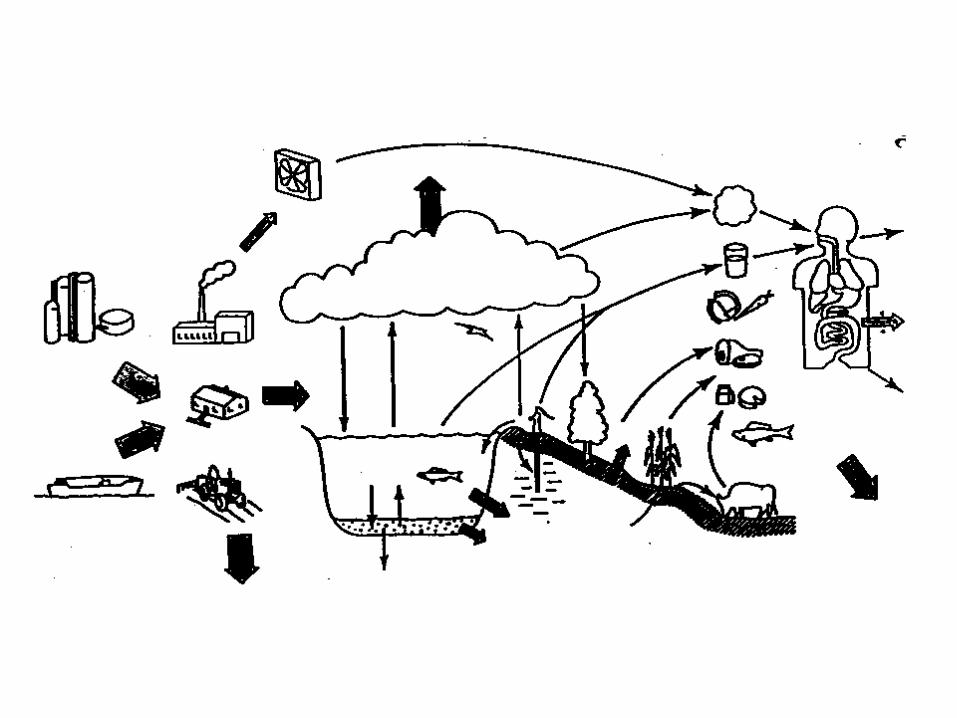
Environmental Fate Models. LEVEL I. Merits To assess multi-media environmental concentrations under more realistic conditions To assess a chemicals’ persistence To assess dominant processes To screen substances for the purpose of ranking. Steady-State & Equilibrium. Cwater. GILL UPTAKE. - PowerPoint PPT PresentationTRANSCRIPT
Environmental Fate Models

LEVEL I


Merits
To assess multi-media environmental concentrations
under more realistic conditions
To assess a chemicals’ persistence
To assess dominant processes
To screen substances for the purpose of ranking
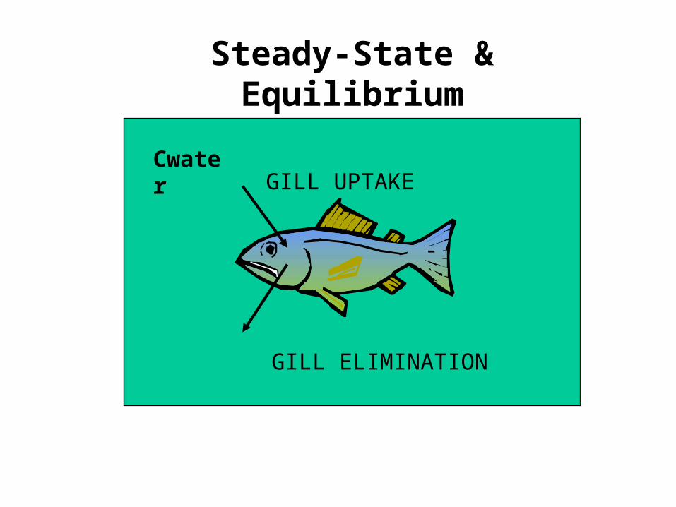
Cwater
Steady-State & Equilibrium
GILL UPTAKE
GILL ELIMINATION
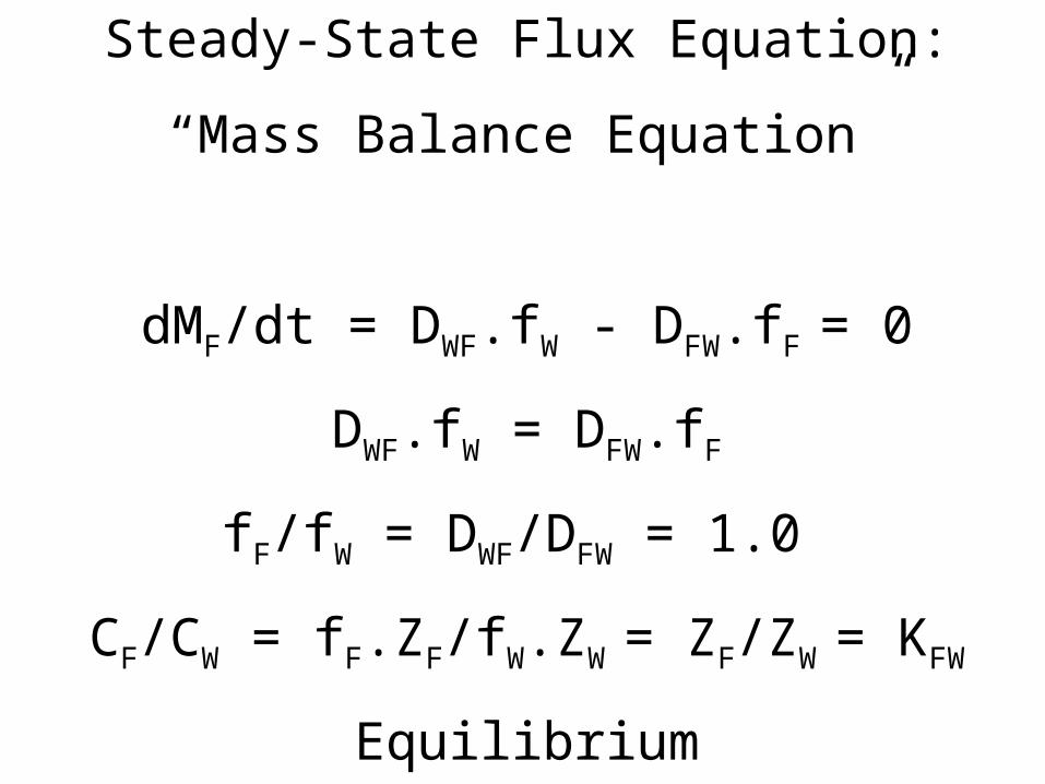
Steady-State Flux Equation:
“Mass Balance Equation”
dMF/dt = DWF.fW - DFW.fF = 0
DWF.fW = DFW.fF
fF/fW = DWF/DFW = 1.0
CF/CW = fF.ZF/fW.ZW = ZF/ZW = KFW
Equilibrium
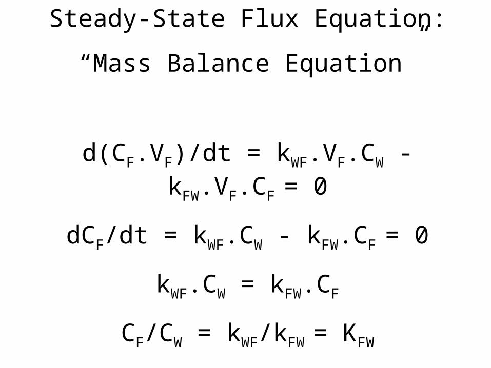
Steady-State Flux Equation:
“Mass Balance Equation”
d(CF.VF)/dt = kWF.VF.CW - kFW.VF.CF = 0
dCF/dt = kWF.CW - kFW.CF = 0
kWF.CW = kFW.CF
CF/CW = kWF/kFW = KFW
Equilibrium

Cwater
Steady-State & Equilibrium
GILL UPTAKE
GILL ELIMINATION
METABOLISM
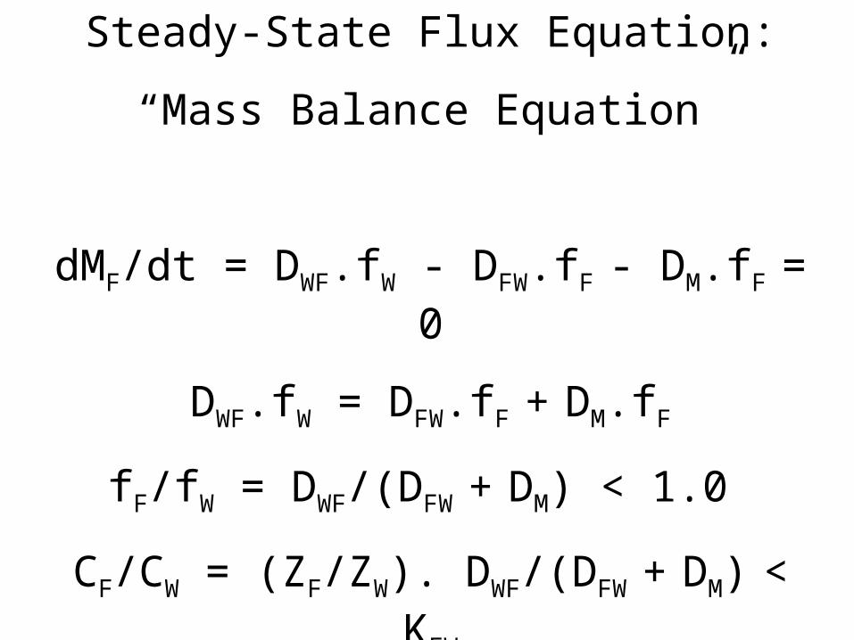
Steady-State Flux Equation:
“Mass Balance Equation”
dMF/dt = DWF.fW - DFW.fF - DM.fF = 0
DWF.fW = DFW.fF + DM.fF
fF/fW = DWF/(DFW + DM) < 1.0
CF/CW = (ZF/ZW). DWF/(DFW + DM) < KFW
Steady-State

Steady-State Flux Equation:
“Mass Balance Equation”
dCF/dt = kWF.CW - kFW.CF - kM.CF = 0
kWF.CW = kFW.CF + kM.CF
CF/CW = kWF/(kFW + kM) < 1.0
CF/CW = kWF/(kFW + kM) < KFW
Steady-State
What is the difference between
Equilibrium & Steady-State?

Question : What is the concentration of chemical X in the water (fish kills?)
Tool : Use steady-state mass-balance model
Lake
CW=?
Volatilisation
Emission
Sedimentation
Reaction
Outflow

Concentration Format
dMW/dt = E - kV.MW - kS.MW - kO.MW - kR.MW
dMW/dt = E - (kV + kS+ kO+ kR).MW
0 = E - (kV + kS+ kO+ kR).MW
E = (kV + kS+ kO+ kR).MW
MW = E/(kV + kS+ kO+ kR) & CW = MW/VW

Fugacity Format
d(VW ZW.fW )/dt = E - DV.fW - DS.fW - DO.fW - DR.fW
dfW/dt = E - (DV + DS+ DO+ DR).fW
0 = E - (DV + DS+ DO+ DR).fW
E = (DV + DS+ DO+ DR).fW
fW = E/ (DV + DS+ DO+ DR) & CW = fW.ZW

Steady-state mass-balance model: 2 Media
Burial
CW=?
Volatilisation
Emission
Settling
Reaction
Outflow
CS=?
Resuspension
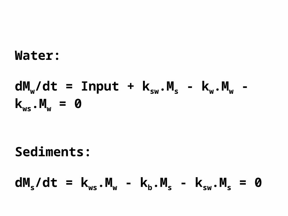
Water:
dMw/dt = Input + ksw.Ms - kw.Mw - kws.Mw = 0
Sediments:
dMs/dt = kws.Mw - kb.Ms - ksw.Ms = 0

From : Eq. 2
kws.Mw = kb.Ms + ksw.Ms
Ms = kws.Mw / (kb + ksw)
Substitute in eq. 1
Input + ksw.{kws.Mw / (kb + ksw)} = kw.Mw + kws.Mw
Input = kw.Mw + kws.Mw - ksw.{kws.Mw / (kb + ksw)}
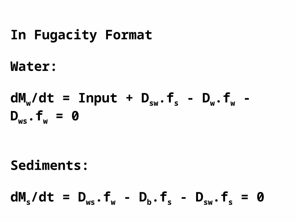
In Fugacity Format
Water:
dMw/dt = Input + Dsw.fs - Dw.fw - Dws.fw = 0
Sediments:
dMs/dt = Dws.fw - Db.fs - Dsw.fs = 0
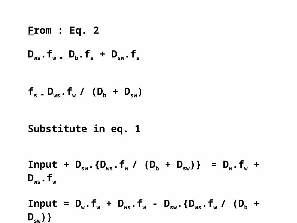
From : Eq. 2
Dws.fw = Db.fs + Dsw.fs
fs = Dws.fw / (Db + Dsw)
Substitute in eq. 1
Input + Dsw.{Dws.fw / (Db + Dsw)} = Dw.fw + Dws.fw
Input = Dw.fw + Dws.fw - Dsw.{Dws.fw / (Db + Dsw)}


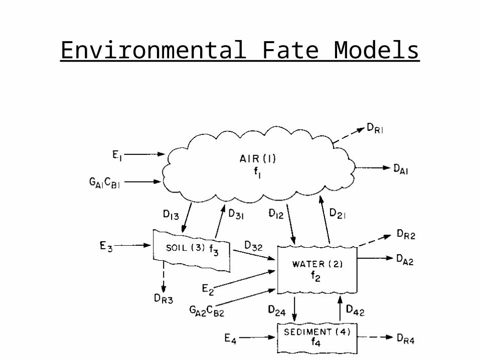
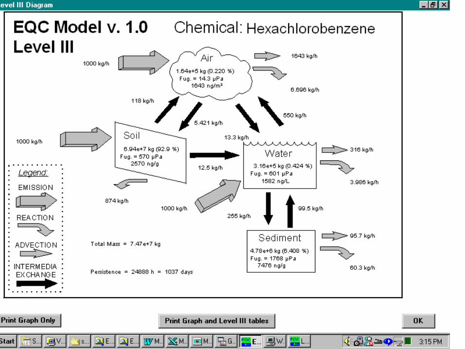
Level III fugacity Model:
Steady-state in each compartment of the environment
Flux in = Flux out
Ei + Sum(Gi.CBi) + Sum(Dji.fj)= Sum(DRi + DAi + Dij.)fi
For each compartment, there is one equation & one unknown.
This set of equations can be solved by substitution and elimination, but this is quite a chore.
Use Computer

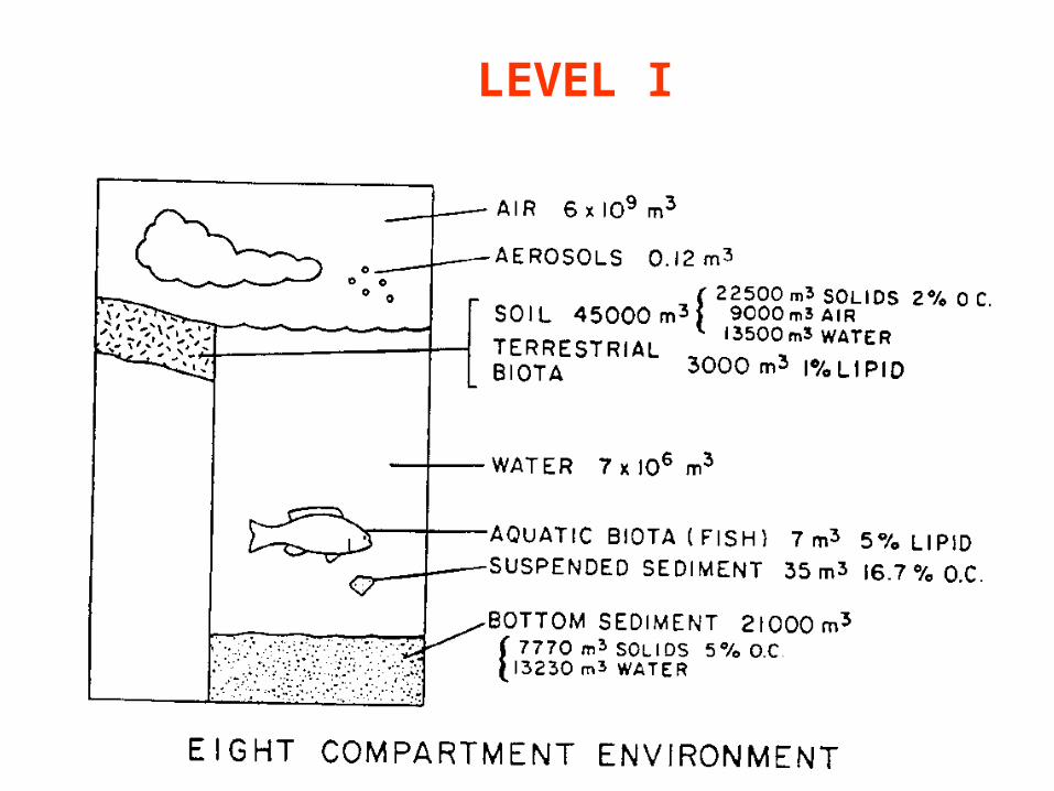
LEVEL I

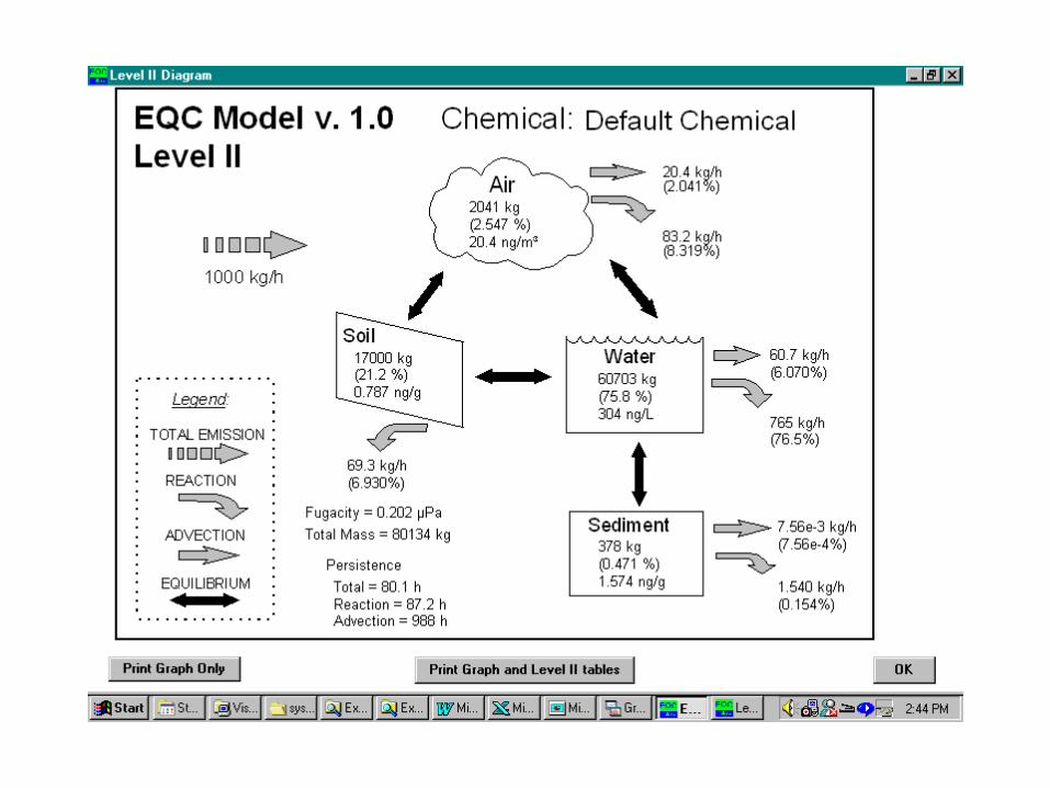
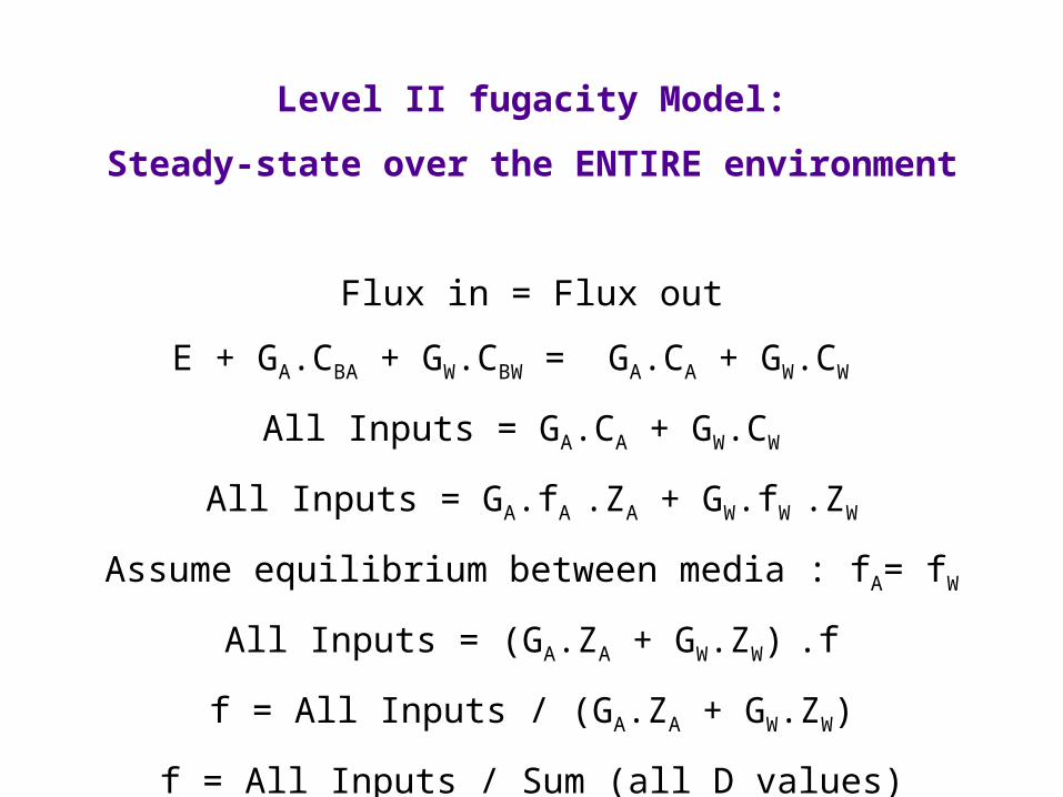
Level II fugacity Model:
Steady-state over the ENTIRE environment
Flux in = Flux out
E + GA.CBA + GW.CBW = GA.CA + GW.CW
All Inputs = GA.CA + GW.CW
All Inputs = GA.fA .ZA + GW.fW .ZW
Assume equilibrium between media : fA= fW
All Inputs = (GA.ZA + GW.ZW) .f
f = All Inputs / (GA.ZA + GW.ZW)
f = All Inputs / Sum (all D values)

Reaction Rate Constant for Environment:
Fraction of Mass of Chemical reacting per unit of time
kR = Sum(Mi.ki) / Mtotal
tREACTION = 1/kR

Removal Rate Constant for Environment:
Fraction of Mass of Chemical removed per unit of time by advection
kA = Sum(Gi.Ci) / Mtotal
tADVECTION = 1/kA

Total Residence Time in Environment:
ktotal = kA + kR = E/M
tRESIDENCE = 1/kTOTAL = 1/kA + 1/kR
1/tRESIDENCE = 1/tADVECTION + 1/tREACTION


Application of the Models
•To assess concentrations in the environment
(if selecting appropriate environmental conditions)
•To assess chemical persistence in the environment
•To determine an environmental distribution profile
•To assess changes in concentrations over time.

Fugacity Models
Level 1 : Equilibrium
Level 2 : Equilibrium between compartments & Steady-state over entire environment
Level 3 : Steady-State between compartments
Level 4 : No steady-state or equilibrium / time dependent

Recipe for developing mass balance equations
1. Identify # of compartments
2. Identify relevant transport and transformation processes
3. It helps to make a conceptual diagram with arrows representing the relevant transport and transformation processes
4. Set up the differential equation for each compartment
5. Solve the differential equation(s) by assuming steady-state, i.e. Net flux is 0, dC/dt or df/dt is 0.
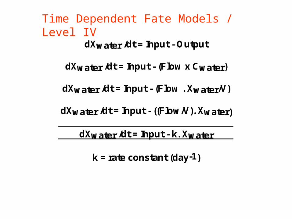
dXwater /dt = Input - Output
dXwater /dt = Input - (Flow x Cwater)
dXwater /dt = Input - (Flow . Xwater/V)
dXwater /dt = Input - ((Flow/V). Xwater)
dXwater /dt = Input - k. Xwater
k = rate constant (day-1)
Time Dependent Fate Models / Level IV

Analytical Solution
Integration:
Assuming Input is constant over time:
Xwater = (Input/k).(1- exp(-k.t))
Xwater = (1/0.01).(1- exp(-0.01.t))
Xwater = 100.(1- exp(-0.01.t))
Cwater = (0.0001).(1- exp(-0.01.t))

0
20
40
60
80
100
120
0 200 400 600 800 1000
Time (days)
Xw
(g
)
Xw ater (g)
Xw ater (g)
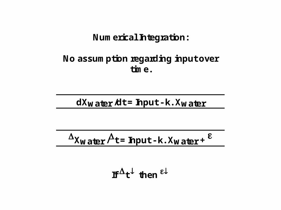
Numerical Integration:
No assumption regarding input overtime.
dXwater /dt = Input - k. Xwater
Xwater /t = Input - k. Xwater +
If t then
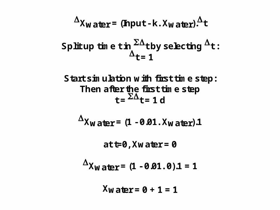
Xwater = (Input - k. Xwater).t
Split up time t in t by selecting t : t = 1
Start simulation with first time step:Then after the first time step
t = t = 1 d
Xwater = (1 - 0.01. Xwater).1
at t=0, Xwater = 0
Xwater = (1 - 0.01. 0).1 = 1
Xwater = 0 + 1 = 1

After the 2nd time stept = t = 2 d
Xwater = (1 - 0.01. Xwater).1
at t=1, Xwater = 1
Xwater = (1 - 0.01. 1).1 = 0.99
Xwater = 1 + 0.99 = 1.99

After the 3rd time stept = t = 3 d
Xwater = (1 - 0.01. Xwater).1
at t=2, Xwater = 1.99
Xwater = (1 - 0.01. 1.99).1 = 0.98
Xwater = 1.99 + 0.98 = 2.97

then repeat last two steps for t/t timesteps
Analytical Num. IntegrationTime Xwater Xwater
(days) (g) (g)0 0 01 0.995017 12 1.980133 1.993 2.955447 2.97014 3.921056 3.9403995 4.877058 4.9009956 5.823547 5.8519857 6.760618 6.7934658 7.688365 7.7255319 8.606881 8.648275
10 9.516258 9.561792

Mass of contaminant in water of lake vs time
0
20000
40000
60000
80000
100000
120000
1 6 11 16 21 26 31 36 41 46 51 56 61 66 71 76
Time (days)
Mas
s in
Lak
e W
ater
(g
ram
s)
Steady-State:Xw = Input/V