environment agent based macroeconomics - hans … · abc de f time (h) time (h) ... knowing in abm...
TRANSCRIPT

AGENT BASED MACROECONOMICS
Stephen Kinsella, University of Limerick and University of Melbourne
FMM Keynesian Summer School, 3 August 2017
Topical articles Agent-based models: understanding the economy 173
Agent-based models: understanding the economy from the bottom upBy Arthur Turrell of the Bank’s Advanced Analytics Division.(1)
Ǧ� �����ǂ����������������������������������������������������������������ƽ������������������������������������������������������������������������������������ǀ
Ǧ� �������������������������������������������������������������ƽ���������������������������������������������Ǐ����������������������������������������������������ǀ�
Ǧ� ������������ƽ������ǂ�������������������������������������������������ƽ��������������������������������ʬ����������������ǩ��������ǎ���������ǏǪ������ƽ��������������������������������������������������������ǀ
Overview
�����ǂ����������������������������������������������������������������������������������������������ǎ�����Ǐ����������ǀ��������������������������������������������������������������������������������ƽ�ʬ�����������������ƽ�������������������ƽ���������������������������������ǀ
����������������������������������������������������������������������������������������������������ǎ���������Ǐ�������������������������������������������������������������������ǀ�����������������������������������������������������������ʬ��������������������������������������������������������������������������ǀ�
�����ǎ������ǂ��Ǐ���������������������������������������������ǎ��������Ǐƽ�����������������������������Ǐ���������������������������������ƽ����������������������������������������������������ǀ���������������������������������������������������ǀ
���������ǂ�������������������������ǂ�����������������������������������������������������������������������������������������������������ƽ��������ƽ����������������������������������ǀ�����������������ƽ������ǂ�������������������������������������������������ƽ����������������������������������ǀ
���������������������������������ƽ���������������������������������������������������ƽ����������������������������������������������ƽ�����������������������������������������������������������������ǀ���������������ƽ����������������������������������������������������������������������������������
���������ǀ���������������������������������������������������������������������������������ǀ
������������������������������ƽ������ǂ���������������������������������������������������������������ƽ������������������������������������������ʬ���������������������ƽ������������������������������ǀ
��������ƽ����������������������������������������ǂ���������������������������ƿ�����������������������������ǀ����������������������������������������������������������������������������ǂ�����������������������������������������������������������������������������������������ƽ�����������������������������������������������������ǀ
ǩȜǪ� ��������������������������������������������������������������������������������������������������ǀ
ENVIRONMENT
Agents Agent-agent interactions Agent-environment interactions
Summary figure Schematic of the typical elements of an agent-based model

5 Ideas Pitfalls & Promise Potential Q&A
20 40 30 20

When you’re bored
(Ideally) Use 3 Colours.For each square on the
page{
Draw a Diagonal Stroke in any direction in any
colourOR
Leave it blank}

5 Ideas


1: BEHAVIOUR DOESN’T NEED EXPLICIT RULES. IT NEEDS
INTENTION & INTERACTION.

AN INTERSECTION IN IRELAND.
2: BEHAVIOUR OFTEN DOESN’T HEED EXPLICIT
RULES, BECAUSE OF IDEA #1.

LOCUSTS

3: UNCOORDINATED BEHAVIOUR CAN APPEAR
COORDINATED

JAPAN’S SHUDAN KOUDOU

4: COORDINATED BEHAVIOUR CAN BE REALLY,
REALLY COORDINATED

SAND PILE EXPERIMENTS

5: MICRO BEHAVIOUR CAN HAVE MACRO EFFECTS
INDEPENDENT OF MICRO LEVEL


SOMETIMES MODELS ARE NOT GOOD REPRESENTATIONS OF
REALITY


Ideas Pitfalls & Promise Potential Q&A
40

Topical articles Agent-based models: understanding the economy 173
Agent-based models: understanding the economy from the bottom upBy Arthur Turrell of the Bank’s Advanced Analytics Division.(1)
Ǧ� �����ǂ����������������������������������������������������������������ƽ������������������������������������������������������������������������������������ǀ
Ǧ� �������������������������������������������������������������ƽ���������������������������������������������Ǐ����������������������������������������������������ǀ�
Ǧ� ������������ƽ������ǂ�������������������������������������������������ƽ��������������������������������ʬ����������������ǩ��������ǎ���������ǏǪ������ƽ��������������������������������������������������������ǀ
Overview
�����ǂ����������������������������������������������������������������������������������������������ǎ�����Ǐ����������ǀ��������������������������������������������������������������������������������ƽ�ʬ�����������������ƽ�������������������ƽ���������������������������������ǀ
����������������������������������������������������������������������������������������������������ǎ���������Ǐ�������������������������������������������������������������������ǀ�����������������������������������������������������������ʬ��������������������������������������������������������������������������ǀ�
�����ǎ������ǂ��Ǐ���������������������������������������������ǎ��������Ǐƽ�����������������������������Ǐ���������������������������������ƽ����������������������������������������������������ǀ���������������������������������������������������ǀ
���������ǂ�������������������������ǂ�����������������������������������������������������������������������������������������������������ƽ��������ƽ����������������������������������ǀ�����������������ƽ������ǂ�������������������������������������������������ƽ����������������������������������ǀ
���������������������������������ƽ���������������������������������������������������ƽ����������������������������������������������ƽ�����������������������������������������������������������������ǀ���������������ƽ����������������������������������������������������������������������������������
���������ǀ���������������������������������������������������������������������������������ǀ
������������������������������ƽ������ǂ���������������������������������������������������������������ƽ������������������������������������������ʬ���������������������ƽ������������������������������ǀ
��������ƽ����������������������������������������ǂ���������������������������ƿ�����������������������������ǀ����������������������������������������������������������������������������ǂ�����������������������������������������������������������������������������������������ƽ�����������������������������������������������������ǀ
ǩȜǪ� ��������������������������������������������������������������������������������������������������ǀ
ENVIRONMENT
Agents Agent-agent interactions Agent-environment interactions
Summary figure Schematic of the typical elements of an agent-based model

–Helbing, 2012
“[ABMs] allow one to start off with the descriptive power of verbal argumentation and to determine the
implications of different hypotheses. From this perspective, computer simulation can provide “an
orderly formal framework and explanatory apparatus”
2.1 Why Develop and Use Agent-Based Models? 31
Location (km)
Location (km)
Location (km)
Location (km)
Location (km)
Location (km)
IDMMLC
0
1
–5
0
050
100
V (km / h)
IDMWSP
Time (h)
IDMSGW
0
1
–5
0
050
100
V (km / h) V (km / h)V (km / h)
V (km / h)V (km / h)V (km / h)V (km / h)
020406080100120140160
IDMHCT
0
1
–5
0
050
100
IDMPLC
0
1
–5
0
050
100
0
1
–5
0
050
100
020406080100120140160
IDMOCT
0
1
-5
0
0 50
100
a b c
d e fTime (h)
Time (h)Time (h)
Time (h)Time (h)
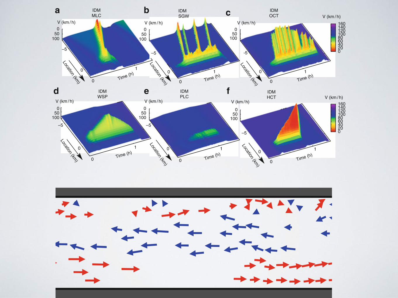
Fig. 2.1 Top: Freeway traffic constitutes a dynamically complex system, as it involves the non-linear interaction of many independent driver-vehicle units with a largely autonomous behaviour.Their interactions can lead to the emergence of different kinds of traffic jams, depending onthe traffic flow on the freeway, the bottleneck strength, and the initial condition (after [27]): amoving cluster (MC), a pinned localized cluster (PLC), stop-and-go waves (SGW), oscillatingcongested traffic (OCT), or homogeneous congested traffic (HCT). The different traffic patternswere produced by computer simulation of a freeway with an on-ramp at location x D 0 km usingthe intelligent driver model (IDM), which is a particular car-following model. The velocity as afunction of the freeway location and time was determined from the vehicle trajectories (i.e. theirspatio-temporal movement). During the first minutes of the simulation, the flows on the freewayand the on-ramp were increased from low values to their final values. The actual breakdown offree traffic flow was triggered by additional perturbations of the ramp flow. Bottom: In pedestriancounterflows one typically observes a separation of the opposite walking directions. This “laneformation” phenomenon has been reproduced here with the social force model [28]
• While pedestrians moving in opposite directions normally organize into lanes,under certain conditions a “freezing-by-heating”effects or intermittent flows mayoccur [38].
• The maximization of system efficiency may lead to a breakdown of capacity andthroughput [30].

–JS Mill, A System of Logic, 1843
“To whatever degree we might imagine our knowledge of the properties of the several ingredients
of a living body to be extended and perfected, it is certain that no mere summing up of the separate actions of those elements will ever amount to the
action of the living body itself.”

184 Quarterly Bulletin 2016 Q4
�������������������������������������������������������������������������������������ǂ���������������������������������������������������Chart 3ǀ���������������������������������������������������������ƽ���������������������������������������������������������������������������������������������������������������������ǩ���Ǫ����������������ǀ�������������������Chart 4ǀ
����������������������������������������������������������������������ǀ��������ƽ�������������ǂ��ǂ������������������������������������������������������������������������������ǀ������������ƽ�����������������������������������������������������������������������������������ȜȠʏ���������������������������������������������������������ȞǀȠ��������������ǩ��������ǂ�����������������������������������ȟǀȠǪǀ��������������������������ƽ�������������������������������������������������������������������������ǀ
The future for agent-based modelling in economics
�����ǂ����������������������������������������ǀ���������������������������������������������������ƽ������������������������������������������������������������������������ǀ��������������������������ƽ�������������������������������������������������������������������������������������������������������ʬ������������������������������������������ǀ
�����������������������������������������������������������������������������������������������������������������������������������������ƽ���������������������������������ǀ
�������������ƽ�����������������������������������������������������������������������������������ʬ�������������������������ǀ�����������������������������������������������������������������������������ƽ�������������ƽ�������������ʬ���������������������������������������ǀ(1)���������������ƽ�����������������������������������ǎ�����Ǐ��������ʬ���������������������������������������������ʬ��ǀ���������������ʬ����������������������������������ǂ�����������������������ǂ��������������������������������������������������������������������������ǀ���������������������������������������������������������������������������������ʬ��������������������������������������������ʬ���������������������ǂ��ǂ���������������������ǩȝǪ�Ǥ�����������������������������������������������ǀ�����������������������������������������������ƽ�����������Go�����Jeopardy!����������������������������ǀ
��������������������������������������������������������������ƽ��������������������������������������������������������������������������������������������������ǂ������������ǀ������������������������������������������������������������������������������������������������������������������������������������������������������������������������������������������ǀ
�����������������������������ƽ����������������������������������������������������������������������ǂ���������������ǀ������ʬ�����������������������������������������������������ǂ�������������������������������ǀ�����������������������������������������������������������������������������������������������������������������������������ǀ���������������������������������������������ʬ��������������ƽ������������������ʬ�����������������������������������������������������������ǀ�������ƽ�������������������������������������������������������������������������������������������������������������������������ǂ�����������ǀ�����������������������ƽ(3)�����������ʬ��������������������������������������������������������������������������������ʬ�����������������ǀ����������ǂ�������������������������������������������������������
Simulation time (years)0 5 10 15 20 25 30 35 40
House price index
0.90
0.95
1.00
1.05
1.10
1.15
1.20
1.25
1.30
Chart 3 A benchmark run of the model showing boom and bust cycles in the house price index
0
5
10
15
20
25
0.0 0.5 1.0 1.5 2.0 2.5 3.0 3.5 4.0 4.5 5.0 5.5 More
Share of total loans, per cent
Loan to income band
Model simulation PSD data
Chart 4 The model can reproduce the loan to income distribution for the United Kingdom
ǩȜǪ� �����������ƽ�����������������������ǩȝțțȜǪǀǩȝǪ� �����������et al�ǩȝțȜȡǪǀǩȞǪ� �����������������������Ǐ�������������������������������������������������������ƽ�
����������������ǀ�������������ǀ��ǀ��Ǡ��������Ǡ���������Ǡ�������Ǡ����ǀ���ǀ
PRECEPTS
• Asynchronous behaviour
• Interactivity
• Mobility
• Distribution
• Non-determinism/emergence

KNOWING IN ABM VS KNOWING IN MAINSTREAM MACRO
• Mechanistic models: hypothesised relationships between agents.
• Nature of the relationship is the data-generating process.
• Parameters often independent of data.
• Detailed microstructures
• Models validated by qualitative comparison, often to patterns in real world.
• Statistical models-Phenomenological, hypothesised relationship between data set variables.
• Relationship seeks ‘best fit’ to data. It is Descriptive.
• Stripped down microstructures
• Validated by quantitative comparison
QUASI-STATISTICAL PROCESSES IN ABM
• Estimation of parameters
• Testing of hypotheses (before and after)
• Covariation/ANOVA type modelling
• Prediction/Forecasting
• Model selection, models within models.

COLEMAN’S BOAT
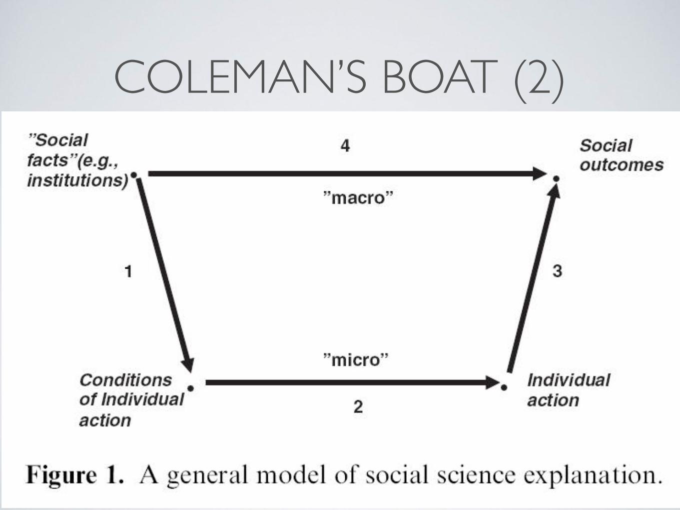
COLEMAN’S BOAT (2)

ABMS IN ECONOMICS
• See Gallegati’s Paradigm Lost (2012) for detailed history, focusing on macro ABMS.
• Schelling’s Model of Segregation —>
0.0 0.2 0.4 0.6 0.8 1.0
0.0
0.2
0.4
0.6
0.8
1.0
0.0 0.2 0.4 0.6 0.8 1.0
0.0
0.2
0.4
0.6
0.8
1.0

AT PROGRAMMATIC LEVEL, ABMS ARE
• Agents
• Rules
• Loops
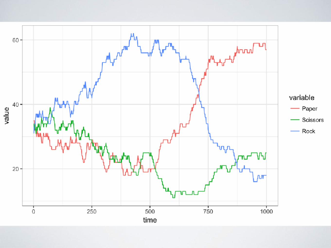
• An example ABM using Rock, Paper, Scissors.
182 Quarterly Bulletin 2016 Q4
Agent-based modelling in the Bank of England
Trading in corporate bonds by open-ended mutual funds(1)
��������ǂ������������������������������������������������������������������������������������������ǂ������������������������������������������������ǀ��������������������������������������������������������������������������������������������������������ǀ
�����������������������������������������������������������������������������������������ȝțțȣ�ʬ��������������ǀ������������������ƽ���������������������������������ʬ���ǂ�������������������������ǀ���������������������������������ƽ����������������������������������������������������������������������ƽ������������������������������������������������������ǀ
������������������������������������������������������������ʬ�����������������ǀ��������������������������������������������������������������������������������������������������������������������������������������ʬ�����������ƽ���������������������������ǀ�������ʬ������������������������������������������ʬ�������ǀ�������������ƽ���������������������������������������������������������������������������ǀ
�����������������������������������������������Figure 6ǀ����������������������������������������������ƽ��������������������������������������������������������ƽ���������������������������������ǀ�������������������������������������������������������������������������������������������������������������ƿ�������������������������������ǂ�������������ǀ�������������������Chart 2ƽ����������������������������������������������������������ǂ��������������������������ǀ������������������������������������������������������������������������ƾ����������������������������������������������������������ʬ���������������������������������������ǀ���������ƽ�������������ʬ���������������������������������������������ǀ
������������������������������������������������������������������������������������ǂ�����������������������������������������������������������������������������ǀ
����������ƽ�������������������������������ƽ�������������������������������������������������������������������������������������������������������������������������������ǀ�����������������������������������ʬ�����������������������������������������ƽ�������������������������������������������������ǀ������������������������������������������������������������������������������ƽ�����������������������������������������������������������������������ǀ�����������������������������������������������������������������������������������������������������������������������������ʬ���ǂ���������������ǀ������������������������������������������������������������������������������������������������������ǀ�
�����������������������������������������������������ǀ���������������������������������������������������������������������������������������������������������������������������������������������������������ǀ
���������������������������Ǐ����������������������������������������������������������������������������ƽ�������������������������������������ǀ��������������������������������������������������������������ǀ����������������������������������������ƽ��������������������������������������������������������������������������������Ǥ�������������������������������������������������������������������ǀ����������������������������������������������������������������������������������������������������������ǀ����������������������������������������������Figure 7ǀ
ǩȜǪ� ���������ǂ���������ƽ�����������������ǩȝțȜȡǪǀ
Corporate bond market
$
Value traders
Momentumtraders Passive funds
Investor
Market makerNoise
Figure 6 Schematic of an agent-based model of the corporate bond market
Daily log-price return8 6 4 2 0 2 4 6 8
10-0Probability densitySimulation
Pre-crisis
– +
10-1
10-2
10-3
10-4
x10-3
CrisisPost-crisis
Chart 2 Reproducing stylised facts: the distribution of daily log-price returns

AB-SFC PAPERS TO CHECK OUT
• Focus on credit and finance:
• EURACE (Deisseberg et al. 2008, Raberto et al. 2012)
• JMAB-Ancona (Caiani et al. 2016, 2017),
• Russo et al., Pisa (Dosi et al. 2010, 2013, 2015, 2017)
• Explicit focus on PK economics:
• Seppecher et al.(2016, 2017) on learning, etc
• Caiani et al. (2016) on credit and endogenous money
• Schasfoort et al. (2017) on monetary policy channels
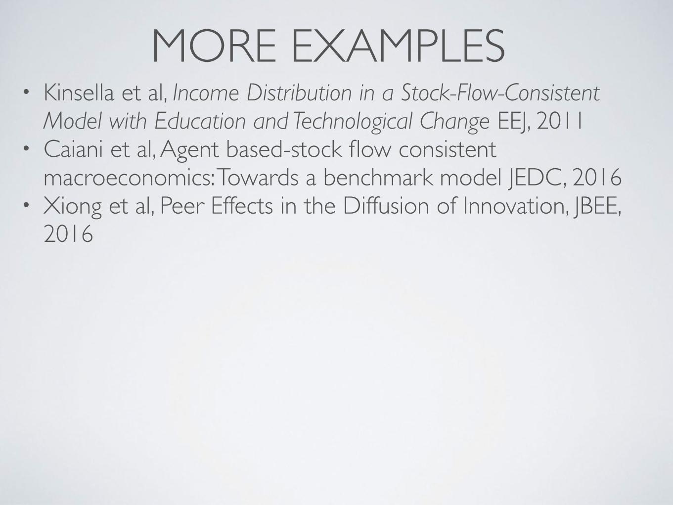
MORE EXAMPLES• Kinsella et al, Income Distribution in a Stock-Flow-Consistent
Model with Education and Technological Change EEJ, 2011• Caiani et al, Agent based-stock flow consistent
macroeconomics: Towards a benchmark model JEDC, 2016• Xiong et al, Peer Effects in the Diffusion of Innovation, JBEE,
2016
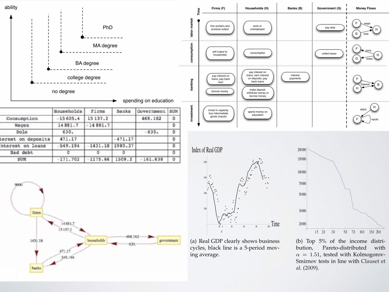
no degree
college degree
BA degree
MA degree
PhD
spending on education
ability
Figure 1: Degree as a function of ability and spending on education.
19
Firms (F) Households (H) Banks (B) Government (G)
Tim
e Money Flows
hire workers and produce output
sell output to households
borrow money
invest in capacity, buy intermediate goods (inputs)
work or unemployed
consumption
make deposit, withdraw money or
borrow money
pay dole
collect taxes
F
HG
wage
dole
HG
F cons.
taxes
pay interest on loans, pay back
loan
pay interest on loans, earn interest
on deposits, pay back loans
interest payments
BH
Finterest
spend money on education
F inputs
Heduc
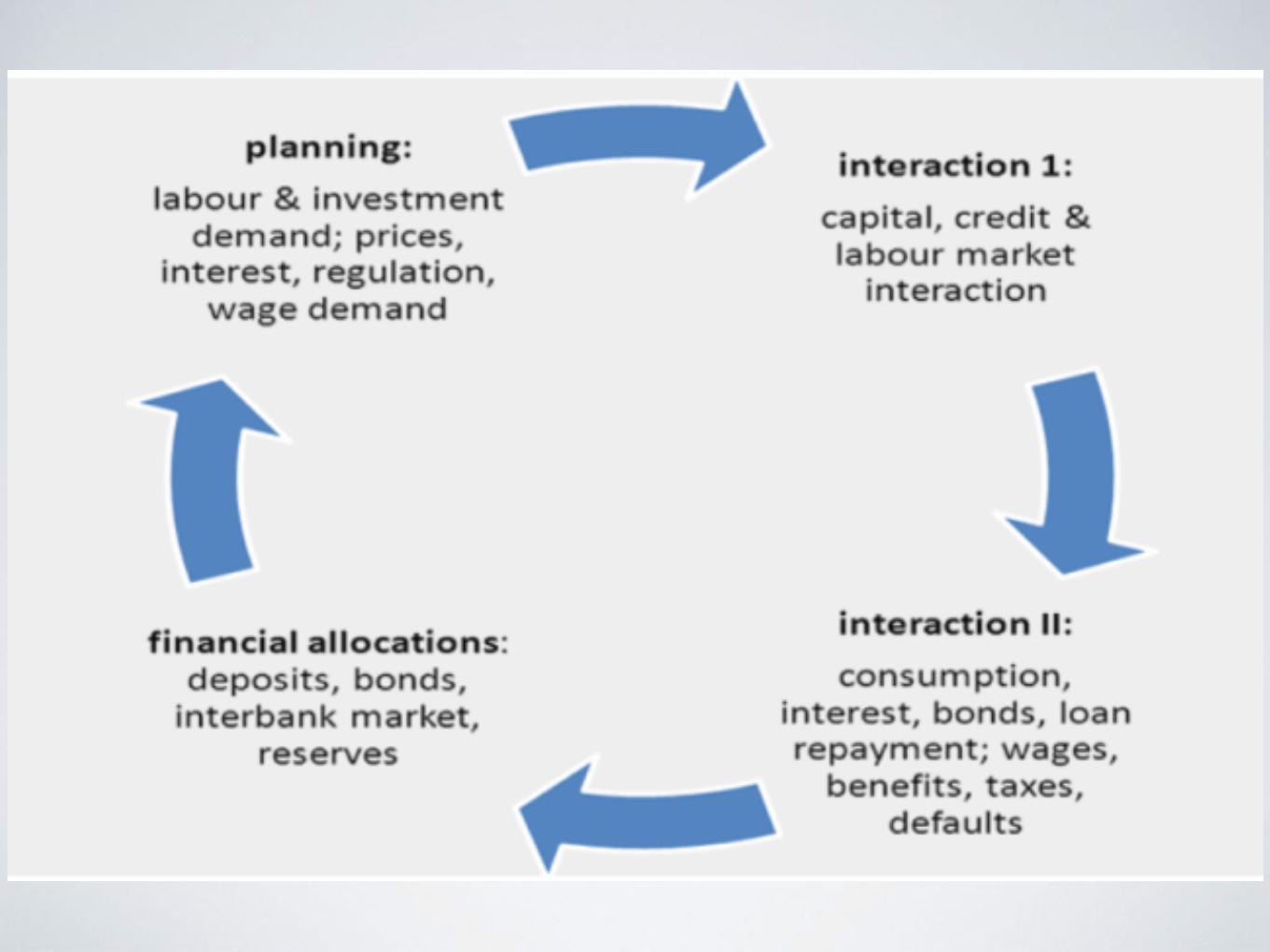
labo
r mar
ket
cons
umpt
ion
bank
ing
inve
stm
ent
Figure 2: Structure of the model.
20
20 40 60 80 100 Time
1300
1400
1500
1600
Index of Real GDP
(a) Real GDP clearly shows businesscycles, black line is a 5-period mov-ing average.
10.05.02.0 20.03.01.5 15.07.0
100000
50000
20000
200000
30000
150000
70000
(b) Top 5% of the income distri-bution, Pareto-distributed with↵ = 1.51, tested with Kolmogorov-Smirnov tests in line with Clauset etal. (2009).
Figure 4: Graphical Output of Simulation Results, 2.
23

Caiani et al, JEDC, 2016.


Fund flows per period

Evolution of Banking Network

Evolution of firm size distribution

Schaasfort (2017): Interbank market

Long Term Dynamics

2 Background and Data 4
Fig. 1: Di↵usion Curve and Income Growth
The ten villages eventually all adopted the new crop mainly due to the fact that seed-stalks, which
can be kept fresh for at most two weeks, were held back from the first year. The initial farmer-innovators,
then, at least to some extent, tried to keep the seed-stalks within only their villages, and within their close
kinship ties. The di↵usion processes in the villages were barely a↵ected by one other, despite the fact
that the villages are geographically close. This was possible also because farming is practised separately
in villages. Land is collectively owned at the village level and distributed to households within a village.
The per capita farmland varies (from 1 mu to over 5 mu) among villages and the size of land plots also
varies significantly. Land plots belonging to di↵erent villages are generally separated by rivers, lakes,
houses or roads. Crucially, infrastructure, mainly in the form of irrigation systems, are owned and run
independently in each village, so in practice very little communication takes place between them.
2.2 Data and Sample Restrictions
2.2.1 Di↵usion Data
We conducted an interview survey over about 10% of households and a questionnaire survey over all
households in each village in 2014 4. In the questionnaire, we asked farmers (mainly the heads of house-
holds) the years in which they started to farm AS and the acreage they farmed each year. Furthermore,
4Refer to Xiong et al. (35) for the dataset we created. It includes the di↵usion data, network data and
demographic data used in this paper.
4 Model and Estimation 10
Fig. 2: Two-layer Multiplex Network
Two approaches are widely adopted to model an agent’s decision making behaviour. One is a
probability-based approach, where an agent’s probability of taking an action (adopting the innovation,
in this case) changes as the proportion of his peers who have taken the action changes (e.g., Banerjee
et al. (4); Peres (29)). The other is a threshold-based approach, wherein an agent takes an action as long
as a certain threshold of the utility is reached (e.g., (17; 30)).
In our case, a household’s likelihood to adopt the new crop increased with the number of family
members who had adopted and the closeness of the kinship ties. This decision making process can be
modelled following the probability-based approach. The probability for a household to adopt is thus
proportional to the sum of the strengths of its kinship ties with those who have adopted. On the
contrary, the externalities that adopting households’ adoption behaviour imposed on non-adopters was
mainly determined by the nature of the crop, such as its compatibility with existing crops. Such influence
thus can be interpreted as a threshold that applies to all households. That is, a household will definitely
adopt once the fraction of its plot neighbours that had adopted reaches a threshold. Therefore, the
externality e↵ect occurring on neighbourhood network is modelled using a threshold.
The agent-based model is a discrete-time model wherein each agent has one of two states at each
time period, adopting or non-adopting. We treat the households who adopted in the first two years (2001
and 2002) as the initial adopters13 or seed adopters. At the beginning of the simulation, the agents
representing the seed adopters are in the adopting state. In each iterate period, the adopting agents
remain in their current state, whereas the non-adopting agents update their adoption states based on
two rules, corresponding to the experience e↵ect or the externality e↵ect, respectively, as follows:
(i) Experience e↵ect In each period, a non-adopter becomes adopting with a probability (elaborated
below). The probability updates according to the proportion of his adopting peers on the kinship
network in last round.
(ii) Externality e↵ect In each period, a non-adopter becomes adopting once the proportion of his
adopting peers on the neighbourhood network reaches a threshold in last period.
The process repeats for a number of periods. In the present case, households’ adoption behaviours
update annually, and the di↵usion process last for 7 years (2003 – 2009). Accordingly, the time period
13In some villages, the first adopters did not appear until 2002. This treatment rules out the possible informa-
tion e↵ect.
Tab. 4: Estimation Results
� ⌘ h(1) (2) (3)
Panel A: Experience Model
Pure Experience E↵ect 4.10Standard Error [0.2569]99% CI of Bootstrap Distribution [3.84, 5.16]
Close Relatives 3.32Standard Error 0.242599% CI of Bootstrap Distribution [2.73, 3.98]
Proximity in Age 4.50 0.275Standard Error [0.2964] [0.1231]99% CI of Bootstrap Distribution [3.72, 5.25] [�0.04, 0.60]†
Panel B: Experience-Externality Model
All Years 3.60 0.30Standard Error [0.2929] [0.2226]99% CI of Bootstrap Distribution [2.83, 4.34] [�0.20, 0.95]
First 4 Years 4.80 0.42Standard Error [0.2979] [0.2339]99% CI of Bootstrap Distribution [3.76, 5.30] [�0.13, 1.08]
Last 4 years 3.10 0.48Standard Error [0.4477] [0.0788]99% CI of Bootstrap Distribution [2.79, 4.88] [0.13, 0.50]
† 95% CI of Bootstrap Distribution is [0.04, 0.52].
Tab. 5: Alternative Fitting of Simulation
� h(1) (2)
Panel A: Lineage Groups
Experience Model 2.70Standard Error [0.2550]99% CI of Bootstrap Distribution [2.43, 3.70]
Experience-Externality Model 1.75 0.68Standard Error [0.2925] [0.2568]99% CI of Bootstrap Distribution [0.82, 2.33] [-0.32, 1.01]
Panel B: Age Groups
Experience Model 4.7Standard Error [0.2463]99% CI of Bootstrap Distribution [4.01, 5.33]
Experience-Externality Model 2.80 0.80Standard Error [0.4346] [0.1424]99% CI of Bootstrap Distribution [2.25, 4.49] [0.45, 1.19]
Xiong et al, 2016

5 Ideas Pitfalls & Promise Potential Q&A
30 20

—@JohnMaeda
“We are surrounded by what looks like something we might need”

INTELLECTUAL ROI
• Econometrics: 50k person-years.
• DSGE, etc: 20k person-years.
• ABM models of all kinds, 500 person-years.
• AB-SFC: 10 person-years (being optimistic)
SUCCESS IS• Doing useful, applied work that influences policy makers by answering important questions.
• How?
• Reproduce correct stylized macro-economic facts
• Exceed performance of DSGE and econometric models?
• Reproduce past events (crises and bubbles)
• Reproduce cross-sectional statistical measures
• Reproduce key time series behaviours
• Provide useful feedback to sub-domains e.g. eliminate some existing theories
• Establish a community of users

SUMMARY: IDEAS
• Behaviour doesn’t need explicit rules. It needs intention & Interaction.
• Behaviour often doesn’t heed explicit rules, because of idea #1
• Uncoordinated Behaviour can appear coordinated
• Coordinated Behaviour Can be Really, Really coordinated
• Micro behaviour can have macro-effects.

TIPS FOR GETTING STARTED
• Don’t use computers. Use whiteboards.
• Start by thinking in terms of agents and behaviour, then build interactions.
• Do the accounting, carefully
• Then code it up.
• A highly non linear process: 20% of paper can take 90% of time

5 Ideas Pitfalls & Promise Potential Q&A
20

AGENT BASED MACROECONOMICS
Stephen Kinsella, University of Limerick and University of Melbourne
FMM Keynesian Summer School, 3 August 2017
Topical articles Agent-based models: understanding the economy 173
Agent-based models: understanding the economy from the bottom upBy Arthur Turrell of the Bank’s Advanced Analytics Division.(1)
Ǧ� �����ǂ����������������������������������������������������������������ƽ������������������������������������������������������������������������������������ǀ
Ǧ� �������������������������������������������������������������ƽ���������������������������������������������Ǐ����������������������������������������������������ǀ�
Ǧ� ������������ƽ������ǂ�������������������������������������������������ƽ��������������������������������ʬ����������������ǩ��������ǎ���������ǏǪ������ƽ��������������������������������������������������������ǀ
Overview
�����ǂ����������������������������������������������������������������������������������������������ǎ�����Ǐ����������ǀ��������������������������������������������������������������������������������ƽ�ʬ�����������������ƽ�������������������ƽ���������������������������������ǀ
����������������������������������������������������������������������������������������������������ǎ���������Ǐ�������������������������������������������������������������������ǀ�����������������������������������������������������������ʬ��������������������������������������������������������������������������ǀ�
�����ǎ������ǂ��Ǐ���������������������������������������������ǎ��������Ǐƽ�����������������������������Ǐ���������������������������������ƽ����������������������������������������������������ǀ���������������������������������������������������ǀ
���������ǂ�������������������������ǂ�����������������������������������������������������������������������������������������������������ƽ��������ƽ����������������������������������ǀ�����������������ƽ������ǂ�������������������������������������������������ƽ����������������������������������ǀ
���������������������������������ƽ���������������������������������������������������ƽ����������������������������������������������ƽ�����������������������������������������������������������������ǀ���������������ƽ����������������������������������������������������������������������������������
���������ǀ���������������������������������������������������������������������������������ǀ
������������������������������ƽ������ǂ���������������������������������������������������������������ƽ������������������������������������������ʬ���������������������ƽ������������������������������ǀ
��������ƽ����������������������������������������ǂ���������������������������ƿ�����������������������������ǀ����������������������������������������������������������������������������ǂ�����������������������������������������������������������������������������������������ƽ�����������������������������������������������������ǀ
ǩȜǪ� ��������������������������������������������������������������������������������������������������ǀ
ENVIRONMENT
Agents Agent-agent interactions Agent-environment interactions
Summary figure Schematic of the typical elements of an agent-based model

LAB~ EXERCISES


LAVOIE: “CHAP03” — 2006/9/11 — 10:03 — PAGE 59 — #3
The Simplest Model with Government Money 59
Table 3.1 Balance sheet of Model SIM
1. Households 2. Production 3. Government !
Money stock +H 0 −H 0
Table 3.2 Accounting (transactions) matrix for Model SIM
1. Households 2. Production 3. Government !
1. Consumption −C +C 02. Govt. expenditures +G −G 03. [Output] [Y]4. Factor income(wages) +WB −WB 05. Taxes −T +T6. Change in the stockof money −!H +!H 0" 0 0 0 0
supply-constrained; it is demand-led. Production responds immediately todemand. Whatever is being demanded will be produced.
3.2.2 Balance sheet and transactions matrix
Model SIM (and every subsequent model) will be introduced with a balancesheet matrix which describes each sector’s stocks of assets and liabilities andtheir logical inter-relationship with those of other sectors – each financialasset owned by one sector always having a counterpart financial liability inone or more other sectors. The balance sheet matrix for Model SIM, given byTable 3.1, is extremely simple as there is only one item – money (H) – whichis a liability of the government and an asset of households. This money isprinted by government: we can assume it consists of banknotes, that is, whatis usually called cash money. Because economists often call this high-poweredmoney, we shall let the letter H stand for it.
Here, as everywhere else, stocks of assets will be entered with a plus signand stocks of liabilities with a minus sign. Since the stock of money is anasset for households – it constitutes their accumulated wealth at a point oftime – it appears with a plus sign (+) in the column allotted to households.On the other hand, the outstanding stock of money constitutes a liability forgovernment. It is the public debt, the debt of government. Thus it is enteredwith a minus sign (−) in the government column.

c_s
g_s
t_s
n_s
yd
t_d
c_d
h_s
h_h
y
n_d
