entropy applications in industrial engineering

University of Nebraska - LincolnDigitalCommons@University of Nebraska - LincolnIndustrial and Management Systems Engineering --Dissertations and Student Research Industrial and Management Systems Engineering

Summer 7-25-2013

ENTROPY APPLICATIONS IN INDUSTRIALENGINEERINGSaeed Zamiri MarvizadehUniversity of Nebraska-Lincoln, [email protected]

Follow this and additional works at: http://digitalcommons.unl.edu/imsediss

Part of the Industrial Engineering Commons, and the Risk Analysis Commons

This Article is brought to you for free and open access by the Industrial and Management Systems Engineering at DigitalCommons@University ofNebraska - Lincoln. It has been accepted for inclusion in Industrial and Management Systems Engineering -- Dissertations and Student Research by anauthorized administrator of DigitalCommons@University of Nebraska - Lincoln.

Zamiri Marvizadeh, Saeed, "ENTROPY APPLICATIONS IN INDUSTRIAL ENGINEERING" (2013). Industrial and ManagementSystems Engineering -- Dissertations and Student Research. 39.http://digitalcommons.unl.edu/imsediss/39

http://digitalcommons.unl.edu?utm_source=digitalcommons.unl.edu%2Fimsediss%2F39&utm_medium=PDF&utm_campaign=PDFCoverPages

http://digitalcommons.unl.edu/imsediss?utm_source=digitalcommons.unl.edu%2Fimsediss%2F39&utm_medium=PDF&utm_campaign=PDFCoverPages


http://digitalcommons.unl.edu/imse?utm_source=digitalcommons.unl.edu%2Fimsediss%2F39&utm_medium=PDF&utm_campaign=PDFCoverPages


http://network.bepress.com/hgg/discipline/307?utm_source=digitalcommons.unl.edu%2Fimsediss%2F39&utm_medium=PDF&utm_campaign=PDFCoverPages

http://network.bepress.com/hgg/discipline/1199?utm_source=digitalcommons.unl.edu%2Fimsediss%2F39&utm_medium=PDF&utm_campaign=PDFCoverPages

http://digitalcommons.unl.edu/imsediss/39?utm_source=digitalcommons.unl.edu%2Fimsediss%2F39&utm_medium=PDF&utm_campaign=PDFCoverPages

ENTROPY APPLICATIONS

IN

INDUSTRIAL ENGINEERING

By

Saeed Zamiri Marvizadeh

A DISSERTATION

Presented to the Faculty of

The Graduate College at the University of Nebraska

In Partial Fulfillment of Requirements

For the Degree of Doctor of Philosophy

Major: Engineering

Under the Supervision of Professor Fred Choobineh

Lincoln, Nebraska

July, 2013

ENTROPY APPLICATIONS

IN

INDUSTRIAL ENGINEERING

Saeed Zamiri Marvizadeh, Ph.D.

University of Nebraska, 2013

Advisor: Fred Choobineh

Entropy is a fundamental measure of information content which has been applied in a

wide variety of fields. We present three applications of entropy in the industrial

engineering field: dispatching of Automatic Guided Vehicles (AGV), ranking and

selection of simulated systems based on the mean performance measure, and comparison

between random variables based on cumulative probability distributions.

The first application proposes three entropy-based AGV dispatching algorithms. We

contribute to the body of knowledge by considering the consequence of potential AGV

moves on the load balance of the factory before AGVs are dispatched. Kullback-Leibler

directed divergence is applied to measure the divergence between load distribution after

each potential move and load distribution of a balanced factory. Simulation experiments

are conducted to study the effectiveness of suggested algorithms.

In the second application, we focus on ranking and selection of simulated systems

based on the mean performance measure. We apply maximum entropy and directed

divergence principles to present a two stage algorithm. The proposed method contributes

to the ranking and selection body of knowledge because it relaxes the normality

assumption for the underlying population which restricts the frequentist algorithms, it

does not assume any priori distribution which is assumed by bayesian approaches, and

finally it provides ranking of systems based on their observed performance measures.

Finally, we present an entropy-based criterion for comparing two alternatives. Our

comparison is based on directed divergence between alternatives’ cumulative probability

distributions. We compare the new criterion with stochastic dominance criteria such as

first order stochastic dominance (FSD) and second order stochastic dominance (SSD).

Since stochastic dominance rules may be unable to detect dominance even in situations

when most decision makers would prefer one alternative over another, our criterion

increases the probability of identifying the best system and reduces the probability of

obtaining the nondominance set in such situations. Among two alternatives, we show that

if one alternative dominates the other one by SSD, the dominating alternative will be

dominated by our new criterion. In addition, we show that the probability associated with

our new criterion is consistent with the probability corresponding to p almost stochastic

dominance (p-AFSD).

i

List of Figures

Figure 1-1. Possible micro-states of each macro-state in die tossing experiment shown

in Abbas (2006) ......................................................................................4

Figure 3-1. Factory layout in Model 1 ..................................................................... 46

Figure 3-2. The factory layout in Model 2 ............................................................... 48

Figure 4-1. Optimal solutions for ��, ��, and �� at the first stage ............................. 67

Figure 4-2. Updated ��, ��, and �� at the second stage ............................................ 68

Figure 5-1. Two possible cases for FSD ................................................................... 77

Figure 5-2. Two possible cases for SSD ................................................................... 78

Figure 5-3. Right and left envelopes of distributions in Figure 5-1 ........................... 82

Figure 5-4. Three different scenarios when ESD is measured ................................... 84

Figure 5-5. distributions set #1: negatively skewed unimodal beta and uniform [0,1]

cumulative distributions ........................................................................ 88

Figure 5-6. Distributions set #2: positively skewed bimodal beta and uniform [0,1]


Figure 5-7. Distributions set #3: positively skewed unimodal beta and uniform [0,1]


Figure AI-1. Input and output queues of work centers at time ��………….......……99

Figure AI-2. Estimated input and output queues of work centers at time t� 3.......99

Figure AI-3. Estimated input and output queues of work centers at time �� 4.5..100

ii

List of Tables

Table 1-1. Some special cases of Csiszer’s directed divergence measure ........... Error!

Bookmark not defined.

Table 1-2. Some generalized measures of directed divergence and their corresponding

measure of entropy ................................................................................. 18

Table 2-1. definitions of different types of flexibility ............................................... 21

Table 2-2. Applications of entropy in different types of flexibility ........................... 23

Table 3-1. Objectives of heuristic dispatching rules................................................. 31

Table 3-2. Operation sequences and production volume percentage of part types. ... 46

Table 3-3. Part types operation times at work centers (minutes) .............................. 47

Table 3-4. Operation sequences and production volume percentage of part types .... 48

Table 3-5. Part types operation times at work centers. ............................................. 48

Table 3-6. Test statistics for the pair-wise T-test ..................................................... 50

Table 3-7. Results of one sided, pair-wise t-tests p-values at 95% level of

significance ............................................................................................ 51

Table 4-1. Initial observations generated from each system under study ................... 65

Table 4-2. Three observations in each bucket and bucket sample means .................. 66

Table 4-3. Simulation results for MDM configuration with increasing variance when

K=3 ........................................................................................................ 71

Table 4-4. Simulation results for MDM configuration with decreasing variance when

K=3 ........................................................................................................ 71

Table 4-5. Simulation results for SC configuration with increasing variance when

K=3 ........................................................................................................ 72

Table 4-6. Simulation results for SC configuration with decreasing variance when

K=3 ........................................................................................................ 72

Table 4-7. Simulation results for MDM configuration with increasing variance when

K=5 ........................................................................................................ 73

Table 4-8. Simulation results for MDM configuration with decreasing variance when

K=5 ........................................................................................................ 73

Table 4-9. Simulation results for SC configuration with increasing variance when

K=5 ........................................................................................................ 74

iii

Table 4-10. Simulation results for SC configuration with decreasing variance when

K=5 ........................................................................................................ 74

Table 5-1. Comparison between SSD and ESD rules on distributions set #1 ............. 88

Table 5-2. computational results for �� ln ��, �� ln ��, �� ln ��, and �� ln �� of

decisions made in Table 5-1 based on ESD, Assuming that � is a

negatively skewed unimodal beta cumulative distribution and � is uniform

[0,1] cumulative distribution. .................................................................. 89



decisions made in distributions set #2 based on ESD, Assuming that � is a

positively skewed bimodal beta cumulative distribution and � is uniform




decisions made in distributions set #3 based on ESD, Assuming that � is a

positively skewed unimodal beta cumulative distribution and � is uniform


Table 5-7. Comparison between probabilities associated with p-AFSD and ESD for

distributions set #1.................................................................................. 95





Table AI-1. Operation sequences, processing times and production volume

percentage of part types …………………………………………………98

Table AI-2. The distance between work centers …………………...………………..98

Table AI-3. Kullback-Leibler Divergence measure calculation for each proposed

algorithm………………………………………………………………..100

iv

Table AII-1. Average waiting time (in minutes) for different configurations of model

1…………………………………………………………………………101

Table AII-2. Average waiting time (in minutes) for different configurations of model

2……………………………………………………………..…………..102

v

Table of Contents

1. Introduction .............................................................................................................1

1-1. Overview of the entropy concept ................................................................2

1-2. Overview of the maximum entropy principle ..............................................6

1-2-1. Maximum entropy in statistical mechanics ..........................................6

1-2-2. Jaynes-Kullback principle of maximum entropy ..................................8

1-3. Kullback-Leibler directed divergence measure ......................................... 11

1-3-1. Relationship with Shannon entropy ................................................... 13

1-3-2. Symmetric divergence ....................................................................... 13

1-4. Generalized measures of entropy and directed divergence ........................ 14

1-5. Outline and contribution ........................................................................... 19

2. Background and literature review ........................................................................... 21

3. Entropy-based dispatching for automatic guided vehicles....................................... 28

3-1. Prior work ................................................................................................ 30

3-2. Applying the Kullback–Leibler divergence measure ................................. 34

3-3. Proposed dispatch algorithms ................................................................... 35

3-3-1. Notation ............................................................................................ 36

3-3-2. Assumptions ...................................................................................... 38

3-3-3. Algorithm one: work content balancing algorithm (WCBA) ............. 38

3-3-4. Algorithm two: output queue balancing algorithm (OQBA) .............. 41

3-4. Comparison with other algorithms ............................................................ 44

3-5. Simulation experiments ............................................................................ 45

3-6. Conclusion ............................................................................................... 51

4. An entropy-based ranking and selection method .................................................... 53

4-1. Preliminaries ............................................................................................ 55

vi

4-2. The proposed R&S algorithm ................................................................... 61

4-3. Numerical example................................................................................... 64

4-4. Simulation experiments ............................................................................ 69

4-5. Conclusion ............................................................................................... 76

5. Entropy-Based measure for stochastic dominance .................................................. 77

5-1. Kullback-Leibler information ................................................................... 79

5-2. Entropy-based criterion for stochastic dominance (ESD) .......................... 81

5-3. Relationship between ESD and FSD, SSD, and p-AFSD .......................... 85

5-4. Conclusion ............................................................................................... 97

Appendix I. A simple numerical example ...................................................................... 98

Appendix II. Waiting time data for different configuration .......................................... 101

Appendix III. Proof of theorems 4.1-4.3 ...................................................................... 103

References ................................................................................................................... 111

1

Chapter 1

1. Introduction

The concept of entropy was introduced by Claude E. Shannon in his 1948 paper "A

Mathematical Theory of Communication". Wikipedia defines entropy as “a measure of

the uncertainty associated with a random variable. In this context, the term usually refers

to the Shannon entropy, which quantifies the expected value of the information contained

in a message, usually in units such as bits and a 'message' means a specific realization of

the random variable. Equivalently, the Shannon entropy is a measure of the average

information content one is missing when one does not know the value of the random

variable.”

Entropy laid the foundation for a comprehensive understanding of communication

theory and according to Kapur and Kesavan (1992), the introduction of Shannon entropy

can be considered as one of the most important breakthroughs over the past fifty years in

the literature on probabilistic uncertainty. The concept of entropy has been applied in a

wide variety of fields such as statistical thermodynamics, urban and regional planning,

business, economics, finance, operations research, queueing theory, spectral analysis,

image reconstruction, biology and manufacturing which will be reviewed in the next

chapter. In this chapter, entropy and two related concepts, maximum entropy and directed

divergence, are reviewed.

2

1-1. Overview of the entropy concept

Entropy of a system can be described in different ways. The original idea was born

from classical thermodynamics. Classical thermodynamics was developed during the 19th

century and its primary architects were Sadi Carnot, Rudolph Clausius, Benoit

Claperyon, James Clerk Maxwell and William Thomson. However, it was Clausius who

first explicitly advanced the idea of entropy. The concept was then expanded by

Maxwell. The specific definition which comes from Clausius, is shown in equation (1-1)

and interprets the entropy, �, as the quantity of heat, �, that is absorbed in a reversible

system when temperature is �.

� � �� 1-1

As long as temperature is constant, it is simple enough to differentiate equation (1-1)

and derive (1-2):

∆� � ∆�� 1-2

Here ∆ represents a finite increment, i.e. ∆� indicates a “change” or “increment” in �,

as in ∆� � �� , where �� and �� are entropies of two different states.

Clausius and the others, especially Carnot, were much interested in the ability to

convert mechanical work into heat energy and vice versa. Hence they interpreted entropy

as the amount of energy in a system that is unavailable to do work. They arrived at

equation (1-3) where ∆� is the energy input to the system, and ∆! is the part of that

energy which goes into doing work.

∆� � ∆U � ∆W� 1-3

3

While physicists were laying the foundations for classical thermodynamics, chemists

interpreted entropy in chemical reactions. Their real interest in entropy was to predict

whether or not a given chemical reaction will take place. They defined entropy as

equation (1-4) in which $ is the enthalpy and � is the free energy (usually known as

Gibb’s free energy).

∆� � ∆H � ∆F� 1-4

In the later 1800’s, Maxwell, Ludwig Boltzmann and Josiah Willard Gibbs, through

the new molecular theory, extended the ideas of classical thermodynamics to a new

domain called statistical mechanics in which each system possesses macro-states and

micro-states. For example, the temperature of a system defines a macro-state, while the

kinetic energy of each molecule in the system defines its micro-state. Equation (1-5), first

derived by Ludwig Boltzmann, is the general form of entropy in statistical mechanics

where '( is the probability that the )*+ particle be in a given micro-state and all '(’s are

evaluated for the same macro-state. , is an arbitrary constant, and in thermodynamics is

the Boltzmann constant which is 1.380658 1 102��.

� � �, 3 '( ln '( 1-5

Mathematical foundations of statistical mechanics are applicable to any statistical

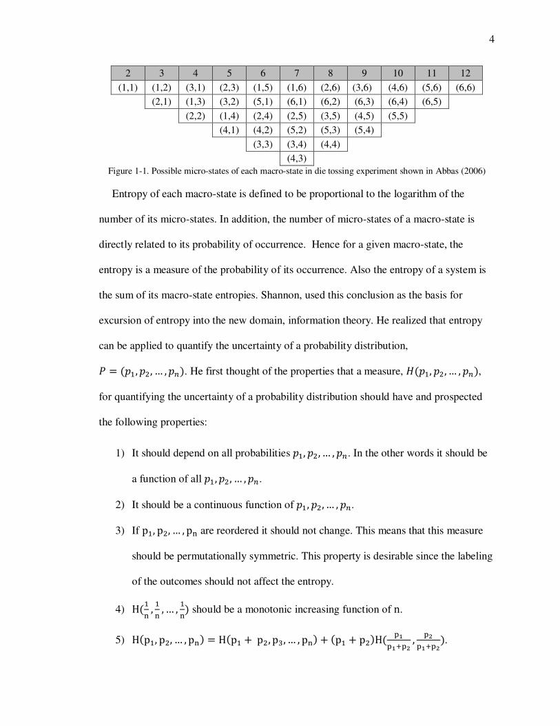
system, regardless of its status as a thermodynamic system. As an example (Abbas, 2006)

consider tossing a die twice. The sum of two throws is considered as a macro-state of this

system and the possible realizations can be considered as micro-states. In this case we

have 11 macro-states (2,3,4,5,6,7,8,9,10,11,12) and 36 microstates. Figure 1-1 shows the

possible micro-states of each macro-state.

4

2 3 4 5 6 7 8 9 10 11 12

(1,1) (1,2) (3,1) (2,3) (1,5) (1,6) (2,6) (3,6) (4,6) (5,6) (6,6)

(2,1) (1,3) (3,2) (5,1) (6,1) (6,2) (6,3) (6,4) (6,5)

(2,2) (1,4) (2,4) (2,5) (3,5) (4,5) (5,5)

(4,1) (4,2) (5,2) (5,3) (5,4)

(3,3) (3,4) (4,4)

(4,3)

Figure 1-1. Possible micro-states of each macro-state in die tossing experiment shown in Abbas (2006)

Entropy of each macro-state is defined to be proportional to the logarithm of the

number of its micro-states. In addition, the number of micro-states of a macro-state is

directly related to its probability of occurrence. Hence for a given macro-state, the

entropy is a measure of the probability of its occurrence. Also the entropy of a system is

the sum of its macro-state entropies. Shannon, used this conclusion as the basis for

excursion of entropy into the new domain, information theory. He realized that entropy

can be applied to quantify the uncertainty of a probability distribution,

� � 4'�, '�, … , '78. He first thought of the properties that a measure, $4'�, '�, … , '78,

for quantifying the uncertainty of a probability distribution should have and prospected

the following properties:

1) It should depend on all probabilities '�, '�, … , '7. In the other words it should be

a function of all '�, '�, … , '7.

2) It should be a continuous function of '�, '�, … , '7.

3) If p�, p�, … , p: are reordered it should not change. This means that this measure

should be permutationally symmetric. This property is desirable since the labeling

of the outcomes should not affect the entropy.

4) H4�: , �: , … , �:8 should be a monotonic increasing function of n.

5) H4p�, p�, … , p:8 � H4p� p�, p�, … , p:8 4p� p�8H4 ;<;<=;> , ;>;<=;>8.

5

Based on these desired properties, Shannon arrived at equation (1-6), which is exactly

the Boltzmann entropy, and pointed out that this is the only measure which satisfies

above properties:

$4'�, '�, … , '78 � �, 3 ') ln ')?

)�1 1-6

where , is an arbitrary positive constant, which satisfies all the properties.

He not only proposed this measure, but also proved the theorem that this was the only

function of '�, '�, … , '7, which had all these properties. In other words, he showed that

these properties characterized this measure.

In addition to the properties illustrated by Shannon, his measure also possesses some

properties which were not initially intended. These additional properties are as follows

(see Aczel and Daroczy (1975) and Mathai and Rathie (1975) for these properties and

their corresponding proofs):

Property 1) The entropy value does not change by adding an impossible event (an

event with zero probability).

Property 2) When this measure is maximized subject to some linear constraints, the

maximizing probabilities are all non-negative.

Property 3) Its value is always positive.

Property 4) Its value is minimum when '�, '�, … , '7 is a degenerate distribution.

Property 5) It is a concave function of '�, '�, … , '7 hence its local maximum will

also be a global maximum.

Property 6) Its maximum value happens for the uniform distribution.

6

Property 7) Additivity: for two independent distributions, the entropy of the joint

distribution, is the sum of the entropies of the two distribution.

Property 8) Strong additivity: for two not necessarily independent distributions, the

entropy of the joint distribution, is the entropy of the first distribution

plus the expected value of the conditional entropy of the second

distribution.

Property 9) Subadditivity: for two not necessarily independent distributions, the joint

entropy is less than or equal to the some of the uncertainties of the two

distributions.

Property 10) The entropy value will be reduced if two outcomes are combined.

1-2. Overview of the maximum entropy principle

The maximum-entropy principle (maxent) originated in statistical mechanics by

Boltzmann (1871c,b,a) and Gibbs (1902). As an approach to density estimation, it was

first proposed by Jaynes (1957b,a), and has since been used in many areas outside

statistical mechanics (Kapur and Kesavan, 1992).

1-2-1. Maximum entropy in statistical mechanics

We begin with the work of Boltzmann (1871c,b,a), who studied properties of gas

bodies, viewed as systems composed of a large number of molecules. One of his central

concerns was how the macro-state of the system is influenced by its micro-states. The

macro-state includes properties such as total volume, total number of molecules, and total

energy. The micro-state is described by the properties of individual molecules such as

their velocities and positions.

7

To simplify the discussion, assume that the molecules of the gas body occupy discrete

states. These can be obtained, for example, by the discretization of positions and

velocities of the molecules. A crucial quantity on both the macro-state and the micro-state

is the energy. The energy of each molecule is the sum of the kinetic energy, which

depends only on the velocity of the molecule, and the potential energy, which depends

only on the position of the molecule within a force field. We assume that the division of

the state space into discrete cells is fine enough so that the energy of molecules within the

same cell is almost constant, but coarse enough to allow a large number of molecules per

cell. The micro-state of the system can be viewed as a vector, listing for each molecule

the cell it occupies. The macro-state is determined by the histogram of molecule counts

across cells. Therefore, to describe the macro-state, it suffices to calculate the most likely

histogram.

Boltzmann applied the “principle of indifference” and assumed that all the micro-

states are equally likely. Thus, the most likely histogram is the one that can be realized by

the largest number of micro-states.

Let’s label the discrete cells as 1, 2, … , A where the number of molecules in the ,*+

cell is BC and the total number of molecules is N. The total number of ways to realize a

concrete allocation into cells is described by equation (1-7)

B!B�! B�! … BF! 1-7

Boltzmann looked for the set of occupancies BC for which the number of possible

realizations equation (1-7) is maximum, while respecting the law of conservation of

energy

8

3 BC�CF

CG� � � 1-8

where EI is the energy associated with the state k and E is the total energy.

Computationally, it is simpler to maximize the logarithm of equation (1-7). The

logarithm of equation (1-7) plays a central role in thermodynamics and when multiplied

by Boltzmann constant, it defines the thermodynamic entropy:

Thermodynamic entropy K ln L!L<!L>!… LM! N 3 BC ln LLOFCG�

Replacing LOL by 'C Boltzmann’s problem can be rephrased as:

Maximize 3 B'C ln 1'CF

CG� 1-9

Subject to the constraint 3 'C�CF

CG� � �B 1-10

Using the method of Lagrange multipliers, we arrive at the solution to Boltzmann’s

problem: the Boltzmann distribution, pI K e`E4I8, where λ is the corresponding

Lagrangian multiplier for equation (1.8) ensuring that the average energy constraint is

satisfied. Using the expression for the Boltzmann distribution, it is now possible to study

various properties of gas bodies.

1-2-2. Jaynes-Kullback principle of maximum entropy

Jaynes (1957b,a) noticed that Boltzmann’s reasoning can be re-interpreted using

information theory and generalized to problems outside statistical mechanics. He

9

suggested that statistical mechanics “may become merely an example of statistical

inference.”

Jaynes, applied the information-theoretic work of Shannon and claimed that

thermodynamic entropy in Boltzmann’s problem can be replaced by information-

theoretic entropy to quantify how uncertain we are about the system. Our only knowledge

about the system is summarized by the average-energy constraint equation (1-10).

Among all distributions satisfying this constraint, we should choose the one that is

“maximally non-committal with regard to the missing information,” i.e., the one with the

largest information-theoretic entropy.

$4�8 � � 3 '( ln '(7

(G�

Since the information-theoretic entropy is a multiple of the thermodynamic entropy,

its maximization yields the result that is identical to Boltzmann’s solution.

Moreover, the principle of maximum entropy can be viewed as a generalization of the

principle of indifference applied by Boltzmann. In statistical inference, the principle of

maximum entopy states that, subject to known descriptive statistics, the probability

distribution which best represents the current state of knowledge, is the one with largest

entropy. In the other words, it chooses the distribution which simultaneously maximizes a

measure of entropy and is compatible with some constraints. If no information is

available, the best probability distribution which is least committed to the information not

given to us is the uniform distribution. Choosing a probability distribution with less value

of entropy means that some data which are not given, are being used. On the other hand,

having a descriptive statistic such as sample mean, maximum entropy principle will

10

construct a probability distribution with the same mean value and the maximum

uncertainty.

Mathematically, this principle implies the maximization of Shannon entropy, subject

to the following constraints.

3 '( � 17(G�

1-11

3 '(cd4e(87(G� � fd , g � 1,2, … , h 1-12

Where i � 4e�, e�, … , e78, c�4i8, c�4i8, … , cj4i8 are functions of i, and

f�, f�, … , fj are related algebraic moment of each function.

The information-theoretic justification of Jaynes was generalized by Kullback (1959)

who assumed that in addition to a set of constraints we are also given a distribution �,

serving as a default guess- the distribution we would choose if we had no data. He

suggested choosing the distribution that is the closest to � among all the distributions

satisfying the constraints. The measure of closeness is the relative entropy,

Ak4�, �8 � 3 '( ln '(l(7

(G� , also known as the Kullback-Leibler divergence, measuring how much information about

the outcome could be gained by knowing P instead of approximating it by Q. If Q is

uniform then the minimum relative entropy criterion is the same as the maximum entropy

criterion.

11

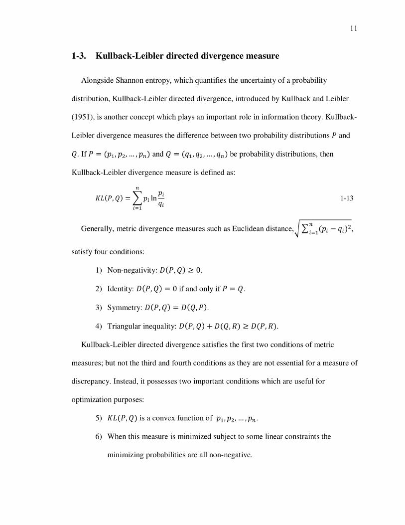
1-3. Kullback-Leibler directed divergence measure

Alongside Shannon entropy, which quantifies the uncertainty of a probability

distribution, Kullback-Leibler directed divergence, introduced by Kullback and Leibler

(1951), is another concept which plays an important role in information theory. Kullback-

Leibler divergence measures the difference between two probability distributions � and

�. If � � 4'�, '�, … , '78 and � � 4l�, l�, … , l78 be probability distributions, then

Kullback-Leibler divergence measure is defined as:

Ak4�, �8 � 3 '( ln '(l(7

(G� 1-13

Generally, metric divergence measures such as Euclidean distance,op 4'( � l(8�7(G� ,

satisfy four conditions:

1) Non-negativity: q4�, �8 r 0.

2) Identity: q4�, �8 � 0 if and only if � � �.

3) Symmetry: q4�, �8 � q4�, �8.

4) Triangular inequality: q4�, �8 q4�, s8 r q4�, s8.

Kullback-Leibler directed divergence satisfies the first two conditions of metric

measures; but not the third and fourth conditions as they are not essential for a measure of

discrepancy. Instead, it possesses two important conditions which are useful for

optimization purposes:

5) Ak4�, �8 is a convex function of '�, '�, … , '7. 6) When this measure is minimized subject to some linear constraints the

minimizing probabilities are all non-negative.

12

Some properties of Kullback-Leibler’s measure are as follows. The corresponding

proofs can be found in Lexa (2004) and Kullback (1959).

Property 1) Ak4�, �8 is a continuous function of '�, '�, … , '7 and of l�, l�, … , l7.

Property 2) Ak4�, �8 is permutationally symmetric, i.e. the value of this measure

does not change if the outcomes are labeled differently if the pairs

4'�, l�8, 4'�, l�8, …, 4'7 , l78 are permuted among themselves.

Property 3) Ak4�, �8 r 0, and is equal to zero if and only if � � �.

Property 4) The minimum value of Ak4�, �8 is zero.

Property 5) Ak4�, �8 is a convex function of both � and �.

Property 6) Since Ak4�, �8 is a convex function of �, its maximum for a given �

must occur at one of the degenerate distributions. The maximum value

has to be

hfe4� t? l� , � t? l� , … . , � t? l78 � t? 1lj(7

where lj(7 � h)? 4l�, l�, … , l78.

Similarly, Ak4�, �8 is a convex function of �, its maximum for a given �

can be made as large as we wish by making some values of l( sufficiently small.

Property 7) When this measure is minimized subject to some linear constraints the

minimizing probabilities are all non-negative.

Property 8) Ak4�, �8 u q4�, �8, i.e., Ak4�, �8 is not symmetric.

Property 9) If � is a priori distribution, � is the probability distribution that

minimizes the cross-entropy subject to the constraints (1-11) and

13

(1-12), and is any other distribution satisfying the same constraints,

then

Ak4s, �8 Ak4�, �8 � Ak4s, �8

1-3-1. Relationship with Shannon entropy

In addition to the above properties, If � is a uniform distribution � � 4�7 , �7 , … , �78,

then

Ak4�, �8 � 3 '(7

(G� ln '(1 ?v � 3 '(7

(G� ln '( ln ? � �$4�8 ln 4?8 Hence,

Ak4�, �8 � �$4�8 w 1-14

Where w � ln ? is constant. Thus, from this perspective, the Shannon entropy measure

can be considered a special case of Kullback-Leibler directed divergence measure,

however they are different conceptually as Shannon entropy is an uncertainty concept;

but Kullback-Leibler divergence measures the directed divergence between to probability

distributions.

1-3-2. Symmetric divergence

As stated in property 8, Kullback-Leibler’s measure, Ak4�, �8, is not symmetric. In

order to define a symmetric divergence measure x4�, �8 can be defined as follows:

x4�, �8 � Ak4�, �8 Ak4�, �8 1-15

This measure is symmetric since x4�, �8 � x4�, �8, obviously. x4�, �8 is called

measure of symmetric cross-entropy or measure of symmetric divergence.

14

1-4. Generalized measures of entropy and directed divergence

However, we noted that Kullback-Leibler measure satisfies conditions (1), (2), (5)

and, (6), there are also other measures that satisfy those four conditions and thus qualify

as legitimate measures of directed divergence. Even if a measure satisfies only conditions

(1), (2), and (5), but not (6), it can still be considered as a measure of directed divergence.

These measures are called generalized measures of directed divergence.

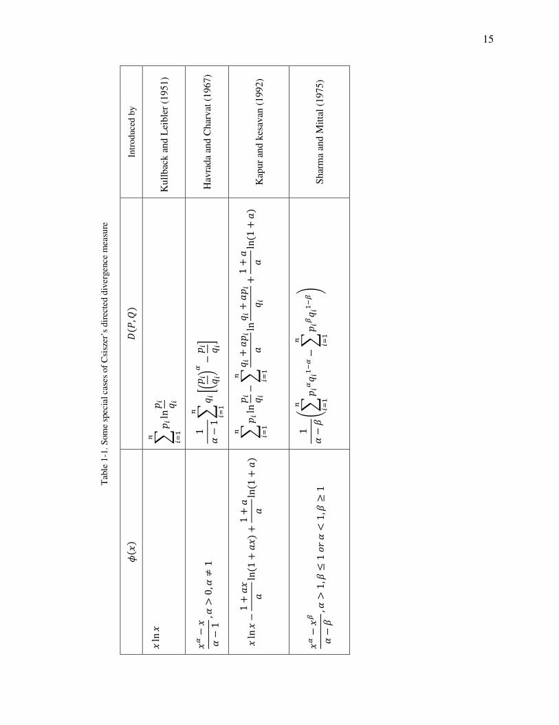
Csiszer (1972), introduced q4�, �8 � ∑ l(z4{|}|87(G� as a family of measures for

directed divergence. In this family z must be a twice differentiable convex function with

z418 � 0. Measure q4�, �8 defined by Csiszer satisfies conditions (1), (2), (5), but not

(6) (See Csiszer,1972).

If z4e8 � e ln e then q4�, �8 � ∑ l( �{|}| ln {|}|�7(G� � ∑ '( ln {|}|7(G� which is Kullback-

Leibler directed divergence. Thus, Kullback-Leibler directed divergence is a special case

of Csiszer’s family of measures when z4e8 � e ln e. Table 1-1shows some special cases

of Csiszer’s directed divergence measure.

15

Tab

le 1

-1. S

ome

spec

ial c

ases

of

Csi

szer

’s d

irec

ted

dive

rgen

ce m

easu

re

Intr

oduc

ed b

y

Kul

lbac

k an

d L

eibl

er (

1951

)

Hav

rada

and

Cha

rvat

(19

67)

Kap

ur a

nd k

esav

an (

1992

)

Sha

rma

and

Mit

tal

(197

5)

q4�,�8

3 ' (ln' ( l (

7 (G�

1 ~�13 l (

� �' ( l (�� ' ( l (�7 (G�

3 ' (ln' ( l (

7 (G��3

l (f' ( f

7 (G�lnl (f

' ( l (1f fln41

f8 1 ~��

�3 '(� l (�2�

7 (G��3

' (� l (�2�7 (G�

�

z4 e8 elne

e� �e ~�1,~�

0,~u1

elne�1f

e fln41fe8

1f fln41f8

e� �e�~��

,~�1,��

1 �g ~�1,�

r1

16

Csiszer family of divergence measures are not defined when l( � 0 and the

corresponding '( u 0. To overcome this problem �� and �� can be defined such that

�� =��=7� and �� =��=7� where f � 0 and � � 0. ��and�� are also probability

distributions and q4��, ��8 � ∑ �}|=��=�7(G� z ��{|=��}|=�� can be used as a measure of directed

divergence of � and �. Thus, the Csiszer family of measures can be generalized by

equations (1-16) and (1-17).

q4�, �8 � 34l( �87(G� z �'( �l( �� , � � 0 1-16

q4�, �8 � 34fl( 187(G� z �f'( 1fl( 1� , f � 0 1-17

The measures presented in Table 1-1 can be generalized by replacing '( by '( � and

l( by l( � or '( by 1 f'( and l( by 1 fl(. For example, generalized forms of

Kullback-Leibler divergence measure would be:

q4�, �8 � 34'( �87(G� ln �'( �l( �� , � � 0 1-18

q4�, �8 � 34f'( 187(G� ln �f'( 1fl( 1� , f � 0 1-19

In addition of being defined even when l( � 0 and the corresponding '( u 0, these

generalized forms give greater flexibility in applications because of the parameters that

they have.

A generalized measure of entropy of a distribution � can be defined as a monotonic

decreasing function of the generalized directed divergence of � from the uniform

distribution. Hence, corresponding to every generalized measure of directed divergence,

17

there is a unique measure of generalized entropy and according to Kapur and Kesavan

(1992), if � � 4�7 , �7 , … , �78 is a uniform distribution, then generalized measures of

directed divergence and entropy are related by equation (1-20).

$4�8 � max q4�, �8 � q4�, �8 1-20

Table 1-2 shows some generalized measures of directed divergence and their

corresponding measure of entropy.

18

Tab

le 1

-2. S

ome

gene

rali

zed

mea

sure

s of

dir

ecte

d di

verg

ence

and

the

ir c

orre

spon

ding

mea

sure

of

entr

opy

$4�8

�3' (ln'

(7 (G�

1 ~�1�3 '

(� �17 (G�

�

�3' (ln'

(7 (G�

�1f? f?ln41

f?831f

?' ( f?ln41

?' (87 (G�

?�2� ��~�3 '

(�7 (G�

�1��?�2� ��~

�3 '(�

7 (G��1�

q4�,�8

3 ' (ln' ( l (

7 (G�

1 ~�13 l (

��' ( l (�� ' ( l (�7 (G�

3 ' (ln' ( l (

7 (G��3

l (f' ( f

7 (G�lnl (f

' ( l (1f fln41

f8 1 ~��

�3 '(� l (�2�

7 (G��3

' (� l (�2�7 (G�

�

19

1-5. Outline and contribution

Although entropy concept has been applied in wide variety of fields (see Kapur

(1993)), there exist even more areas where it can be employed. In this work we study

applications of entropy in industrial engineering. Three problems are addressed and for

each problem an entropy-based approach is suggested.

In the first problem we address the dispatching issue of a material handling system

within the context of Automatic Guided Vehicles (AGV) in a discrete part manufacturing

system. The dispatching issue is about allocating available AGVs to move requests to

ensure efficient part flow in the factory. We believe that the objective of this resource

allocation problem should be load balancing among the factory work centers. Using

Kullback-Leibler directed divergence, we present entropy-based resource allocation

algorithms that consider the consequence of potential moves on the load balance of the

factory before resources are allocated. The proposed algorithms are suitable for real-time

implementation and strive to even the load in the factory while satisfying the move

requests generated by the factory work centers.

In the second problem we focus on ranking and selection based on the mean

performance measure. We use maximum entropy and Kullback-Leibler directed

divergence principles to present a two stage algorithm for this problem. The proposed

method contributes to the ranking and selection body of knowledge because it relaxes the

normality assumption for underlying population which restricts the frequentist

algorithms, it does not assume any priori distribution assumed by bayesian methods, and

finally it provides ranking of systems based on their observed performance measures.

20

Finally, we present an entropy-based criterion for comparing two alternatives. Our

comparison is based on directed divergence between alternatives’ cumulative probability

distributions. We compare the new criterion with stochastic dominance criteria such as

first order stochastic dominance (FSD) and second order stochastic dominance (SSD).

Since stochastic dominance rules may be unable to detect dominance even in situations

when most decision makers would prefer one alternative over another, our criterion

reduces the probability of obtaining the nondominance set in such situations. Among two

alternatives, we show that if one alternative dominates the other one by SSD, the

dominating alternative will be dominated by our new criterion. In addition, we show that

the probability associated with our new criterion is consistent with the probability

corresponding to p almost stochastic dominance (p-AFSD).

The remainder of this dissertation is organized as follows. Chapter 2 reviews the

applications of entropy in industrial engineering and specially manufacturing context.

Entropy-based dispatching algorithms for automatic guided vehicles are presented in

chapter 3. Ranking and selection via simulation is studied in chapter 4 and the new

entropy-based ranking and selection procedure is offered. Chapter 5, focuses on the

stochastic dominance issue. An entropy-based measure for stochastic dominance is

introduced in this chapter.

21

Chapter 2

2. Background and literature review

Soon after entropy and maximum entropy concepts were introduced by Shannon and

Jaynes respectively, they began to be used in wide variety of fields such as statistical

thermodynamics, urban and regional planning, business, economics, finance, operations

research, queueing theory, spectral analysis, image reconstruction, biology and

manufacturing (see Kapur (1993) for some applications).

Within Manufacturing, the entropy concept has been applied to measure diversity of

production systems from two different points of views: Flexibility and Complexity.

a) Flexibility

Flexibility is defined as the ability of a system to cope with changes (Mandelbaum,

1990). Sethi and Sethi (1990) defined different types of flexibility as shown in Table 2-1.

Table 2-1. definitions of different types of flexibility

Flexibility Definition

Machine Various types of jobs can be performed by machine

Operation Different ways can be used to perform a job

Process Different parts can be made without a major setup

Routing A part can be produced through different routes

Volume Different overall output levels can be produced

Market The system can easily adapt itself with market changes

Production Different parts can be produced without adding major capital equipment

Program System can be run unattended for a period of time

Material handling Different parts can be moved efficiently through a manufacturing facility

Product New products can be added or substituted easily

Expansion Capability and capacity can be increased easily

22

Entropy has been widely used to measure and quantify flexibility in manufacturing

systems. A system facing uncertainty uses flexibility as an adaptive response to cope

with changes. The flexibility in the action of the system depends on the decision options

or the choices available and on the freedom with which various choices can be made

(Kumar, 1987). A greater number of choices leads to more uncertainty of outcomes, and

hence, increased flexibility. According to Pereira and Paulre (2001), the level of

flexibility of a system depends on the set of possible outcomes and therefore possible

ways that these outcomes can be obtained. This inference has been the main driver to

apply entropy as a measure of flexibility by different researchers. Thus for all the

proposed measures, the possible states of the system and their related probabilities of

occurrence is defined. Entropy concepts are then applied to the obtained probability

distribution to measure flexibility.

Yao (1985), and Yao and Pei (1990) applied entropy to the measurement of the

routing flexibility of a flexible manufacturing system. Kumar (1987, 1988) adopted it for

the measurement of operation flexibility. Chang et al. (2001) suggested that two attributes

of flexibility, namely routing efficiency and routing versatility, should be considered in

the measurement models of routing and single-machine flexibility. Chang (2007)

proposed a multi attribute approach for routing flexibility by considering three attributes:

routing efficiency, routing versatility and routing variety. Chang (2009) offered a multi

attribute approach for machine-group flexibility. Rao and Gu (1994) used entropy as a

means of measuring production volume and production flexibility. Shuiabi et al. (2005)

applied entropy as a measure of the flexibility of production operations. Extended from

Yao and Pei’s approach (Yao and Pei, 1990), Piplani and Wetjens (2007) proposed two

23

dispatching rules, namely ‘least reduction in entropy’ and ‘least relative reduction in

entropy’ for operations dispatching based on entropic measures of part routing flexibility.

Table 2-2 shows the proposed entropy measures of flexibility and their related flexibility

type.

Table 2-2. Applications of entropy in different types of flexibility

Flexibility Entropy-based approach

Machine Chang et al. (2001), Chang (2009)

Operation Shuiabi et al. (2005)

Process ----

Routing Chang (2007), Piplani and Wetjens (2007), Yao (1985), Yao and Pei (1990)

Volume Chang (2004), Rao and Gu (1994), Olivella et al. (2010)

Market ----

Production Rao and Gu (1994)

Program ----

Material handling ----

Product ----

Expansion ----

a) Complexity

Complexity can be associated with systems that are difficult to understand, describe,

predict or control. As noted by Scuricini (1987) who states that: “Complexity is a

subjective quality, its meaning and its value change following the scope of the system

being taken under consideration”, it is difficult to define complexity in a precise formal

sense.

Generally, the complexity of a system can be described in terms of several

interconnected aspects of the system such as: number of elements or sub-systems, degree

24

of order within the structure of elements or sub-systems, degree of interaction or

connectivity between the elements, sub-systems and the environment, level of variety, in

terms of the different types of elements, sub-systems and interactions, and degree of

predictability and uncertainty within the system.

Authors have analyzed complexity in two different aspects: structural complexity

which is associated with the system configuration (Deshmukh, 1993; Deshmukh et al.,

1998) and operational complexity which is defined as the uncertainty associated with the

dynamical aspects while system is running (Frizelle and woodcock, 1995; Scuricini,

1987; Sivadasan el al., 2002).

Entropy provides a means of quantifying complexity. The complexity of a system

increases with increasing levels of disorder and uncertainty. Therefore, a higher

complexity system requires a larger amount of information to describe its state.

According to the entropy concept, the structural complexity is thus defined as the

expected amount of information (entropy) necessary to describe the state of a planned

system; while operational complexity is defined as the expected amount of information

necessary to describe the state of the system’s deviation from the schedule.

The idea of using entropy as a measure for complexity in manufacturing was first

introduced by Frizelle and Woodcock (1995), and Frizelle (1996), for operational

complexity. Calinescu et al. (1998) applied and assessed the operational complexity

measures offered by Frizelle and Woodcock (1995), and Frizelle (1996). Deshmukh

(1993), and Deshmukh et al. (1998) used entropy to suggest an entropy-based measure

for structural complexity. Frizelle and Suhov (2001) offered some measures for both

structural and operational complexities. Sivadasan et al. (2002) offered an entropy-based

25

methodology to measure the operational complexity of supplier-customer systems

associated with the uncertainty of material and information. Fujimoto et al. (2003)

applied entropy to study structural complexity because of product variety. They used this

measure to manage assembly process design strategies. Yu and Efstathiou (2006)

introduced entropy-based operational complexity as a new way to assess the performance

for rework cells. Martinez-Olvera (2008) proposed an entropy formulation to assess

information sharing approaches in supply chain environments. Sivadasan et al. (2006)

modeled the operational complexity of supplier-customer systems from an information-

theoretic perspective. Wu et al. (2007) studied the relationship between cost and the

operational complexity measures offered by Frizelle and Woodcock (1995). Sivasadan et

al. (2010) studied the effect of closer supply chain integration on operational complexity

of production scheduling.

In addition to manufacturing, the entropy concept has been applied in different fields

within decision making under uncertainty context including portfolio selection and

measures of risk.

- Portfolio selection

Portfolio selection is about assigning a certain amount of wealth to different assets so

that the investment can bring a most profitable return. Markowitz (1952) proposed the

mean-variance (M-V) analysis model and created a fundamental basis for modern

portfolio analysis. M-V model tries to maximize the expected return for a given level of

risk or to minimize the level of risk for a given level of expected return. The portfolio

variance decreases as portfolio diversification increases. Entropy has become a well-

established measure of diversification. Higher portfolio diversification yields a greater

26

entropy value. Bera and Park (2005, 2008) applied entropy and cross entropy to provide a

well-diversified portfolio. Huang (2008) introduced two types of fuzzy mean-entropy

models. Zhang et al. (2009) considered a multi-period portfolio selection problem by

taking into account four criteria: return, risk, transaction cost, and diversification degree

of portfolio. They offered a possiblistic mean-semivariance entropy model in which

entropy is applied to measure diversification degree of portfolio. Jana et al. (2009)

considered the portfolio selection problem by taking into account four criteria and added

entropy as the objective function to generate a well diversified asset. Qin et al. proposed

three portfolio selection methods based on fuzzy cross-entropy. Wu et al. (2009) applied

the maximum entropy principle to obtain a numerical solution for their min-max model to

investigate the optimal portfolio with riskless assets. Rodder et al. (2010) used an

information theoretical inference mechanism under maximum entropy and minimum

cross entropy principles, respectively, in order to propose an entropy-driven expert

system for portfolio selection. Bhattacharyya (2013) offered a fuzzy portfolio selection

model by minimizing mean-skewness as well as minimizing variance- cross entropy.

- Measures of risk

According to Jones and Zitikis (2007), a risk measure is a mapping from the set of all

random variable to the extended real numbers in order to quantify the degree of risk

involved in each random variable. Although many authors have proposed suitable

methods to measure risk in the past two decades, entropy applications to measure risk

have been constrained to a limited number of research studies.

Yang and Qiu (2005) introduce the expected utility entropy (EU-E) measure of risk

and suggest a decision-making model based on expected utility and entropy. The EU-E

27

reflects an individual’s intuitive attitude toward risk while the decision model

incorporates the expected utility decision criterion as a special case. Föllmer (2011)

proposes a new coherent risk measure called the iso-entropic risk measure, which is

based on cross entropy under the theory framework of Artzner et al.(1999). Ahmadi-Javid

(2012) introduces the concept of entropic value-at-risk (EVaR), a new coherent risk

measure that corresponds to the tightest possible upper bound obtained from the Chernoff

inequality for the value-at-risk (VaR) as well as the conditional value-at-risk (CVaR).

Chengli and Yan (2012) study a coherent version of the entropic risk measure, both in the

law invariant case and in a situation of model ambiguity.

28

Chapter 3

3. Entropy-based dispatching for automatic guided vehicles

Material handling is a nonvalue adding, necessary function for the production of

discrete parts. It entails moving work in progress among work centers and raw material

into and finished products out of the factory. Inefficient implementation of material

handling could substantially add to production costs. For example, delays in work-in-

process movement would increase parts’ factory flow time, resulting in higher inventory

costs. Therefore, efforts have been made to improve both the technology and efficient

implementation of material handling systems.

An Automatic Guided Vehicle System (AGVS) is an example of a material handling

system that has benefited from technological innovation and has created opportunities to

improve the efficiency of material movement. An AGVS is considered by many as the

most flexible automated material handling system (Hwang and Kim, 1998). This

flexibility stems from the intelligence imbedded in the AGVS and on board of each

automated guided vehicle (AGV). This intelligence allows the system to be responsive, in

real time, to the material move requests generated by the work centers.

Operation control of an AGVS consists of resolving vehicle routing, vehicle

dispatching, and vehicle scheduling issues. A routing issue (Kim and Tanchoco, 1991;

Nishi et al., 2005; Nishi et al., 2009) is identifying the best path for the assigned AGV. A

dispatching issue (Egbelu and Tanchoco, 1984; Kim and Klein, 1996; Hwang and Kim,

1998; Ho and Chein, 2006) is assigning AGVs to pickup or delivery requests. A

scheduling issue (Zaremba et al., 1997; Sabuncuoglu, 1998; Veeravalli et al., 2002; Gaur

29

et al., 2003) is determining the arrival or departure times of AGVs at pickup or delivery

points. Each of these control issues has its own relevant objective(s) that myopically

could be optimized. However, an AGVS controller must contribute toward optimizing the

objectives of the factory, since material handling is a supporting function within a

factory. An important objective for factory management is minimization of the time that

parts spend in the factory, i.e., parts flow time. The material handling system can

contribute to achieving the factory objective by addressing work center move requests in

a timely manner while avoiding creation of temporary bottlenecks or aggravating

structural bottlenecks. Temporary bottlenecks are created when workload is not properly

distributed among the work centers, and structural bottlenecks are aggravated when a

scarce capacity of work centers is ignored when dispatching decisions are made.

In this chapter, we focus on the dispatching issue of a material handling system

within the context of an AGVS in a discrete part manufacturing system. Since the

dispatching issue is about allocating available AGVs to move requests to ensure efficient

part flow in the factory, the objective of this resource allocation solution is load balancing

among the factory work centers. Specifically, we use an entropy-based resource

allocation rule that considers the consequence of potential moves on the load balance of

the factory before resources are allocated. The proposed approach is suitable for real-time

implementation and strives to even the load in the factory while satisfying the move

requests generated by the factory work centers.

The remainder of this chapter is organized as follows. In Section 3.1, we present a

brief review of prior work. The application Kullback–Leibler divergence measure is

explained in Section 3.2. Three dispatching algorithms are proposed in Sections 3.3. In

30

Section 3.4, performance of proposed algorithms is studied and compared with other

algorithms by conducting simulation experiments. Finally, conclusions and future

research directions are presented in Section 3.5.

3-1. Prior work

Dispatching is a resource allocation problem in that idle AGVs (resource) are assigned

to move requests (demand). At a given time, the resource vector consists of a possibly

ordered list of idle AGVs, and the demand vector consists of a possibly ordered list of

move requests. The problem is to determine the one-to-one pairing of the elements of

these two vectors.

AGV dispatching rules have been investigated by many researchers. Simple heuristic

dispatching rules are discussed by Egbelu and Tanchoco (1984). They divided the

dispatching rules into two categories: work-center-initiated (mapping from the demand

vector to the resource vector) and vehicle-initiated (mapping from the resource vector to

the demand vector) rules and showed that in busy production settings vehicle-initiated

dispatching rules are preferable. Their vehicle-initiated category consists of the following

rules: random work center (RW); shortest travel time/distance (STT/D); longest travel

time/distance (LTT/D); maximum outgoing queue size (MOQS); minimum remaining

outgoing queue size (MROQS); modified first-come, first-served (MFCFS); and unit load

shop arrival time (ULSAT). Each of these heuristic rules optimizes an objective. These

objectives are summarized in Table 3-1.

31

Table 3-1. Objectives of heuristic dispatching rules

Heuristic Rule Objective

RW Maximizing long term dispatching entropy STT/D Minimizing the percentage of vehicles’ time/distance empty travel LTT/D Maximizing the percentage of vehicles’ time/distance empty travel MOQS Minimizing the percentage of time parts spend in output queue

MFCFS Minimizing the elapsed time between placing a move request by work center and its satisfaction

MROQS Minimizing the possibility of work center blockage ULSAT Minimizing the percentage of time parts spend in input queues

Bartholdi and Platzman (1989) propose a decentralized dispatching rule for a simple

closed-loop system. Their suggested rule, First Encountered, First Served (FEFS), assigns

the AGV traveling along the loop to the move request it encounters first. The basis of this

rule is to minimize the percentage of AGV empty travel time. Yamashita (2001) suggests

two dispatching policies: “the nearest vehicle in time” and “the nearest vehicle in

distance.” The objective of these rules is to minimize the AGV empty travel time. Kim et

al. (2004) propose two dispatching rules for a single-loop, single vehicle AGV system:

MAED (Minimum Average of Empty Distance) and MSED (Minimum Sum of Empty

Distance). The MAED rule minimizes the average vehicle travel time, and the MSED

rule minimizes the sum of AGV vehicle travel time.

Some authors have extended single-objective dispatching rules to multiobjective

decision rules by considering several decision criteria recognizing, due to

interdependencies within a manufacturing process, some objectives may have conflicts.

In general, multiobjective dispatching rules are supposed to perform better than single-

objective rules. Kim and Hwang (1999) propose an AGV dispatching rule based on three

bidding functions defined for travel time, input buffer size, and output buffer size. The

objective is to minimize a combination of these three bidding functions. Naso and

32

Turciano (2005) suggest a hierarchical fuzzy dispatching rule in which, if a critical move

request (e.g., requests from work centers with a saturated output buffer or directed to

starved destinations) is detected, it is selected as the final decision. Otherwise, a

multicriteria rule is called with the objective of optimizing the AGV utilization by

minimizing the empty vehicle travel time. Tan and Tang (2001) suggest an AGV

dispatching rule to strike a compromise between satisfaction of several simple objectives

using a hybrid Fuzzy-Taguchi approach. Bozer and Yen (1996) develop two algorithms,

Modified Shortest Travel Time First (MOD STTF) and Bidding-Based Dynamic

Dispatching (B2D2). The basis of these policies is to minimize the empty vehicle travel

time. Kim and Klein (1996) propose several multiattribute decision rules and compare

them with the single-attribute dispatching rules for different performance measures.

Jeong and Randhawa (2001) propose a multiattribute dispatching rule by considering the

unloaded travel distance to the pickup point, the remaining space in the input buffer of

the delivery point and the remaining space in the outgoing buffer of the pickup point.

Guan and Dai (2009) offer a deadlock-free multia-attribute dispatching method by

considering three criteria: traveling distance, input queue size and output queue size.

These criteria are weighted and combined into a single criterion. Criteria are weights

influenced by transportation loads and processing loads.

The objectives of most of the proposed dispatching rules in the literature are

optimization of material handling rather than factory performance measures. Since a

material handling system has a supporting role in the factory, its control should be

aligned with optimizing the factory’s performance. A highly desirable performance

objective of a factory is to achieve a laminar flow of parts within the factory. The notion

33

of laminar flow has been of much interest in operation of assembly lines and has led to

the creation of a large body of knowledge generally known as assembly line balancing

(e.g., Stecke, 1983; Mukhopadhyay et al., 1992; Becker and Scholl, 2006). The promise

is that when factory work centers (or assembly line work centers) are balanced in work

content, no work center is overburdened or starved; and thus the flow of parts through the

factory is smooth.

We propose a look-ahead AGV dispatching approach that considers the contribution

of a potential material move to the laminar flow within the factory before an AGV is

dispatched. The only prior work which considers the factory load balancing concept

when dispatching decisions are made is Kim et al. (1999). They define a balancing index

based on the difference between the number of parts in the pickup and the destination

work centers. Their rule selects the job with the highest balancing index. Their decision is

based on the current state of the system, while they do not consider the resulting state

after the dispatched AGV delivers the parts to the destination. Since movement of parts

into or out of the system or among work centers impacts the state of the system, we take

into consideration the impact of making such moves as we plan an AGV’s dispatch.

Hence, in this research, the resulting state of the system after each possible dispatching

decision is predicted, and the dispatch decision that contributes the most to the laminar

flow of the factory is selected. The Kullback–Leibler divergence principle is used to

measure the contribution of a dispatch toward the system laminar flow, and simulation

experiments are conducted to compare the performance of the proposed approach with

three simple dispatching rules: Shortest Travel Distance (STT), Maximum Outgoing

Queue Size (MOQS), and Modified First-Come, First-Served (MFCFS).

34

3-2. Applying the Kullback–Leibler divergence measure

We represent the work content of work centers at a given time by a vector whose

elements are the existing work content in each work center. Moving a work load between

two work centers changes the work content vector. Under the ideal balanced factory

operating conditions, elements of the work content vector should be equal at all times.

Manufacturing system literature suggests that a balanced production system has the

highest throughput, that is, bottlenecks are avoided (laminar flow). This notion of

balanced factory gives us an ideal benchmark, although a practical utopia, for operating a

factory.

We utilize this notion of balanced factory as our reference vector and order the move

requests based on the distance of their resultant workload vector from the balanced

factory work content vector. The move request that results in a workload vector closest to

the balanced factory vector is deemed to be the best move at the time of the dispatch

decision.

If elements of the work content vector are represented as a proportion of the total work

content of the factory, then the work content vector can be viewed as a probability

distribution. Under this scenario, the work content vector of an ideal factory is a uniform

distribution. Therefore, determining the distance between the resultant work content

vector of a move request and the ideal work content vector becomes determining the

degree of divergence between two probability distributions.

We will apply the Kullback-Leibler directed divergence measure explained in chapter

1 to tackle this problem. As mentioned in chapter 1, their measure, measures the directed

35

divergence between a probability distribution,�, and a reference distribution, �. If

� � 4'�, … , '78 and the reference distribution is � � 4l�, … , l78, then Ak4�, �8 �∑ '( ln �{|}|�7(G� . Moreover, Ak4�, �8 � 0 if, and only if, � � �. When the reference

probability distribution is uniform, i.e., l( � l � ), then Ak4�, �8 � �$4�8 ln 4?8.

The first term of Ak4�, �8 is the Shannon entropy, and the second term is a constant.

Thus, when operation utopia is a balanced factory, it suffices to calculate the Shannon

entropy of the potential resultant work content distributions and select the dispatch that

has the largest Shannon entropy.

3-3. Proposed dispatch algorithms

A dispatch action reduces the number of parts in the output queue of the originating

work center and increases the number of parts in the input queue of the receiving work

center by the same amount. Increasing the size of a work center’s input queue increases

the work content of the work center, while reducing the size of the output queue does not

impact the work content of the work center. Additionally, process completion of a part at

a work center which results in moving the part to the output queue changes the work

content of the work center. In general, the addition of parts to an input queue of a work

center has a greater impact on the work content of that work center than moving one or

more parts to the output queue of the work center. The primary reason is that batches of

parts are moved into the input queue, and single parts are moved into the output queue.

In this section, we present three algorithms for a dispatching decision. The first

algorithm attempts to balance the factory work content among all work centers by

assessing the impact of increasing the work content of a work center after a dispatch.

36

The second algorithm attempts to balance the number of loads in the output queue of

work centers by assessing the impact of removing a load from the output queue of a work

center. The third algorithm attempts to balance the combined number of loads in the input

and output queues of the work centers by assessing the impact of a potential dispatch on

the factory balance. Algorithms two and three may be considered work content balancing

algorithms, rather than number of load balancing algorithms, if the work content of all

loads in the factory is the same. For all three algorithms, the base reference is an ideal

factory where work content or number of loads are uniformly distributed among the work

centers. Before we present the algorithms, we define the notations used in the algorithms

and state the assumptions under which the algorithms were developed.

3-3-1. Notation

B{: Number of part types

B�: Number of work centers

B�: Number of vehicles

�: Vehicle speed

w: Vehicle capacity

k�: Vehicle loading time

��: Vehicle unloading time

�4t, )8: Mean service time of part type t at work center ) �q: An B� 1 B� matrix where �q�,( is the distance between the drop-off point of

work center � to pickup point of work center )

37 q�: An B� 1 B� matrix where q��,( is the distance between the pickup point of

work center � to drop-off point of work center ) ��: Arrival rate of part t into the system

��(}*: Number of undispatched and unassigned parts of type t in the output queue

of work center ) that is requested to be moved to the input queue of work

center q at time �

��(*: Number of undispatched and unassigned parts at the output queue of work

center ) at time �, ��(* � ∑ ��(}*L��G�

�*: Set of move requests at time �, �* � ��(}*|��(}* � 0¡

¢£�(* : Estimated number of parts of type t at the input queue of work center ) at

time �

¤¥�(*: Estimated number of parts of type t at the output queue of work center ) at time �

¤¥(*: Estimated number of parts at the output queue of work center ) at time �,

¤¥(* � ∑ ¤¥�(*L��G�

!(*+4¦, ��8: The §*+ waiting position of part type ¦ that arrived at time �� at the

input queue of work center ) at observed time �

¨�(*+ 4�{, ?8: The arrival time, �{, at the output queue of work center ) of the §*+

vehicle dispatched at time � to pick up ? units of part type t

38 ©�(*+ 4�� , ?8: The arrival time, ��, at the input queue of work center ) of the §*+

vehicle dispatched at time � to deliver ? units of part type t ��(} : Estimated system entropy if part type t is moved from output queue of work

center ) to the input queue of work center q

3-3-2. Assumptions

The following assumptions are used:

1) All AGVs are single load vehicles.

2) The factory layout and AGVS guide paths are known.

3) The number of AGVs available in the system is known.

4) Number and location of pickup and delivery points are known and fixed.

5) An idle AGV stays at the work center of last delivery before being

dispatched.

6) AGV failure time is negligible.

7) The longest idle AGV will be assigned to a dispatch first.

Assumption 7 expresses the work-center-initiated rule which will be applied if more

than one AGV is idle at a given time.

3-3-3. Algorithm one: work content balancing algorithm (WCBA)

Suppose a vehicle is idle at location � at time ��, and ª�*«ª u 0 move requests have

been made. Let ��(} be the total time required to complete move request ��(}*« and �� (} be the clock time when it is completed. For each move request ��(}*« ¬ �*«, the

expected work content of work centers at time �� (} is computed. The algorithm

39

selects the move request that results in the work content of work centers to be as equal as

possible (closest to an ideal factory).

The pseudo code of WCBA consists of the Main procedure and the Work Content

Estimation procedure. The Work Content Estimation procedure calculates the work

content of work centers at the completion time of each requested move.

WCBA: Main Procedure

The Main procedure consists of four steps. Step 1 identifies �*«, the set of move

requests at time ��. Step 2 first calculates the total time required to complete each move

request. Then the Work Content Estimation procedure is called to compute the expected

number of part types at the input queues of work centers at the move request completion

time. Finally, the work content of the work center is calculated and system entropy is

obtained. In Steps 3 and 4, respectively, the move request with the largest entropy

measure is chosen as the best dispatch decision and a vehicle is dispatched.

Step 1. Identify the set of move requests at time ��, �*«.

Step 2. For each move request ��(}*« ¬ �*«:

• Compute ��(} � �®,|¯ k� �|,°¯ ��,

• Call Work-Content-Estimation procedure to compute ¢£±C,*«=²³|° for all ¦ ¬ �1, … , B{¡ and , ¬ �1, … , B�¡,

• Compute ��(} � � ∑ ´ ∑ µ4±,C8.¶£·O,¸«¹º³|°»�·¼<∑ ∑ µ4±,½8.¶£·¾,¸«¹º³|°»�·¼<»¿¾¼< ln ∑ µ4±,C8.¶£·O,¸«¹º³|°»�·¼<∑ ∑ µ4±,½8.¶£·¾,¸«¹º³|°»�·¼<»¿¾¼< ÀL¿CG� .

Step 3. Set 4t�, )�, l�8 � �fe��(}¡ . Step 4. Dispatch the vehicle to the work center )� to pickup part type t�.

40

WCBA: Work-Content-Estimation Procedure

Work Content Estimation procedure is a subprocedure which is called by the Main

procedure to compute ¢£±C,*«=²³|°. Step 1 compares the number of parts of type t at the

output queue of work center ) with w, the vehicle capacity, to find, the number of parts �

that can be moved. Step 2 checks whether there are any dispatched vehicles to deliver

parts to the input queue of work center , before move completion time �� (} . If a

!C*« � !C*« Á Á Â4¦, ��8, . . . , 4¦, ��8ÃÄÄÄÄÅÄÄÄÄÆ7 ÇÈ·O¸«É 4*�,78¬Ê·±¬Ë�,...,L�Ì

Step 1. Set � � �)?Íw, ¤Î�(*« Ï.

Step 2. Υ± � Ë©±C*«+ 4�� , ?8ª�� (}Ì, ¦ ¬ Ë1, . . . , B{Ì, ¢£±,C,*«=²³|° � ¢±C*« ∑ ?È·O¸«É 4*®,78¬Ê· ,

Step 3. If , � 1, then for each part type ¦ with mean interarrival time �Ñ· generate ?±

interarrival times ¨�· , … , ¨7· such that ∑ ¨j·7·j·G� � ��(} . Set !C*« � !C*« Á Í¦, ∑ ±̈Òj·dG� ÏÓj·¬Ë�,…,7·ÌÓ±¬Ë�,…,L�Ì and sort it by the ascending arrival

time.

Set ¢£±C,*«=²³|° � ¢£±C,*«=²³|° ?±.

Step 4. Set � � ��.

Step 5. If ∑ ¢£±C,*«=²³|°L�±G� � 0 set � � ��|!C*« �4¦, ��8 and go to Step 6, or else go to Step 7.

Step 6. If � � �� (}, then ¢£±|ÔO¸«<4±,*Õ8,C,*«=²³|° � ¢£±|ÔO¸«<4±,*Õ8,C,*«=²³|° � 1,

� � � �4,, ��|!C*« �4¦, ��88, !C*« � !C*«/Ë!C*«�4¦, ��8Ì, and go to Step 5, or else go to Step 7.

Step 7. If , � l then, ¢£�C,*«=²³|° � ¢£�C,*«=²³|° �.

41

move could be accomplished, then the number of parts and ordered set of parts waiting to

be processed at the input queue of this work center are updated. If work center , is the

work center at which parts enter the system, Step 3 computes the expected number and

the order of parts which enter the input queue of this work center during the move

completion time. The number of parts and ordered set of parts waiting to be processed at

the input queue of work center , are also updated in this Step. Steps 4, 5, and 6 calculate

the number of parts that will be processed from time �� to time �� (} . Finally, if work

center , is the work center to which the parts will be transported, Step 7 updates the

number of parts at the input queue of the work center by adding � units of parts to it.

3-3-4. Algorithm two: output queue balancing algorithm (OQBA)

OQBA looks at the number of parts at the output queues of work centers and selects a

move request in which the output queue sizes become closest to each other. The Main

procedure of this algorithm is similar to that of WCBA; but instead of balancing the work

content, it tries to balance the output queue sizes. Hence, the only difference in the Main

procedure takes place at the second step, as shown below:

Step 2 of OQBA: Main Procedure


• Compute �4�,(,}8 � �®,|¯ k� �|,°¯ ��,

• Call Number In Queue Estimation procedure to compute ¤¥C,*«=²³|° for

all , ¬ �1, … , B�¡,

• Compute ��(} � � ∑ ´ ×¥O,¸«¹ º³|°∑ ×¥·,¸«¹ º³|°»¿·¼< ln ×¥O,¸«¹ º³|°∑ ×¥·,¸«¹ º³|°»¿·¼< ÀL¿CG� .

42

Number in Queue Estimation procedure is a subprocedure inside the Main procedure.

Step 1 verifies that the number of parts of type t that are to be moved from the output

queue of work center ) does not exceed the vehicle capacity. Step 2 checks if there are

any dispatched vehicles to pick up parts from the output queue of work center , before

move completion time �� (}. If such vehicles exist, the scheduled number of parts to

pick up is deducted from the output queue of work center , at the scheduled pickup time.

Step 3 checks if there are any dispatched vehicles to deliver parts to the input queue of

work center , before move completion time, �� (} . If there are any, then the number

of parts and ordered set of parts waiting to be processed at the input queue of this work

center are updated. Step 4 computes the expected number and the order of parts which

enter the input queue of work center , during the move completion, if , is a work center

at which parts enter the system. The number of parts and the ordered set of parts waiting

to be processed at the input queue of work center , are then updated in this step. Steps 5,

6, and 7 calculate the number of parts that will be processed from time �� to time �� (} . If work center , is the work center to which parts are moved, Step 8 updates the

number of parts at its input queue by adding � units of parts to it. Finally, the number of

parts processed by work center , during move completion time, is added to the number

of parts at its output queue at Step 9. The pseudo code of the Number in Output

Estimation procedure is as follows:

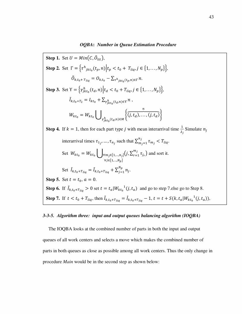
43

OQBA: Number in Queue Estimation Procedure

3-3-5. Algorithm three: input and output queues balancing algorithm (IOQBA)

The IOQBA looks at the combined number of parts in both the input and output

queues of all work centers and selects a move which makes the combined number of

parts in both queues as close as possible among all work centers. Thus the only change in

procedure Main would be in the second step as shown below:

!C*« � !C*« Á Â4¦, ��8, . . . , 4¦, ��8ÃÄÄÄÄÅÄÄÄÄÆ7 ÇÈ·O¸«É 4*® ,78¬Ø

Step 1. Set � � �)?Íw, ¤Î�(*Ï,

Step 2. Set Γ � Ú¨+±C*«4�{, ?8��{ � �� (} , ¦ ¬ Ë1, . . . , B{ÌÛ, ¤¥C,*«= ²³|° � ¤C,*« � ∑ ?ÜÉ·O¸«4*� ,78¬Ý .

Step 3. Set Υ � Ú©±C*«+ 4��, ?8�� (} , ¦ ¬ Ë1, . . . , B{ÌÛ, ¢£C,*«=²> � ¢C*« ∑ ?È·O¸«É 4*® ,78¬Ê ,

Step 4. If , � 1, then for each part type ¦ with mean interarrival time �Ñ· Simulate ?±

interarrival times ¨�· , … , ¨7· such that ∑ ¨j·7·j·G� � ��(} . Set !C*« � !C*« Á Í¦, ∑ ±̈Òj·dG� ÏÓj·¬Ë�,…,7·ÌÓ±¬Ë�,…,L�Ì and sort it.

Set ¢£C,*«=²³|° � ¢£C,*«=²³|° ∑ ?±L�±G� .

Step 5. Set � � ��, f � 0.

Step 6. If ¢£C,*«=²³|° � 0 set � � ��|!C*«�4¦, ��8 and go to step 7.else go to Step 8.

Step 7. If � � �� (} , then ¢£C,*«=²³|° � ¢£C,*«=²³|° � 1, � � � �4,, ��|!C*« �4¦, ��88, !C*« � !C,*«/Ë!C*« �4¦, ��8Ì f � f 1

44

Step 2 of IOQBA: Main Procedure

IOQBA Number in Queue Estimation procedure is the same as OQBA Number in

Queue Estimation procedure.

In the Appendix IV, a simple numerical example demonstrates the steps of the

proposed algorithms.

3-4. Comparison with other algorithms

In this section, the performance of the three proposed algorithms is compared with the

following dispatching rules.

Shortest Travel Time (STT) rule: If a vehicle is idle at location � at time �� and

ª�*«ª u 0 move requests have been made, the decision is to dispatch the vehicle to the

�4�,(,}8 � � Þ3 � ¤¥C,*«=²³|°∑ ¤¥±,*«=²³|°L¿±G� ∑ ¢£±,*«=²³|°L¿±G� ln ¤¥C,*«=²³|°∑ ¤¥±,*«=²³|°L¿±G� ∑ ¢£±,*«=²³|°L¿±G� �L¿CG�

ß


• Compute �4�,(,}8 � �®,|¯ k� �|,°¯ ��,

• Call Number in Queue Estimation procedure to compute ¤¥C,*«=²³|° and ¢£C,*«=²³|° for

all , ¬ �1, … , B�¡,

• Compute:

ß∑ ´ ¶£O,¸«¹º³|°∑ ×¥·,¸«¹º³|°»¿·¼< =∑ ¶£·,¸«¹º³|°»¿·¼< ln ¶£O,¸«¹º³|°∑ ×¥·,¸«¹º³|°»¿·¼< =∑ ¶£·,¸«¹º³|°»¿·¼< ÀL¿CG� à.

45

move request ��(�}�*« such that ��(�}� � Min ��(}¡, where ��(} is the total time required

to accomplish the move request ��(}*« .

Maximum Outgoing Queue Size (MOQS) rule: If a vehicle is idle at location � at

time �� and ª�*«ª u 0 move requests have been made, the decision is to dispatch the

vehicle to the move request ��(�}�*« such that ��(�*« � Max��(*«¡ and ��(�}�*« �Max��(�}*« ¡.

Modified First Come First Served (MFCFS) rule: When a part becomes available at

the output queue of a work center and no vehicle is free at that time, the time that the

request was generated is saved. When a vehicle becomes available, it is assigned to the

work center with the earliest saved request time. Also, each work center can have at most

one saved request at a time.

3-5. Simulation experiments

To evaluate the performance of the proposed algorithms, two simulation models are

developed. Experiments are conducted using different system parameters for each model

including: number of vehicles, vehicle capacity, and parts arrival rates to the system.

Model 1: Figure 3-1 shows the factory layout for the first model. This factory

consists of 11 work centers. Parts enter the system from Work Center 1 and exit from

Work Center 11. The pickup and drop-off points (circles) are arranged in a way so that

when a vehicle is approaching a work center, it will reach the work center’s drop-off

point first. Five part types are produced in the factory. Table 3-2 shows the operation

sequence and production volume percentage of each part type. It is assumed that each

part type has a fixed process time at each work center. The processing time of each part

46

type at each work center is illustrated in Table 3-3. The average vehicle speed is 150 feet

per minute and it takes 0.5 minute to perform loading or unloading operations.

Simulation experiments are conducted using different values for number of vehicles (4 or

5), vehicle capacity (5, 20 or unlimited), and mean interarrival time of parts to the factory

(4.6, 4.8, 5, 5.2, 5.4, 5.6, 5.8 or 6 minutes). Parts arrival to the factory is exponentially

distributed. Initial simulation test runs show that the factory will be oversaturated when

the mean interarrival time is smaller than 4.6 minutes.

Figure 3-1. Factory layout in Model 1

Table 3-2. Operation sequences and production volume percentage of part types.

Part Type Operation Sequence Production Volume

Percentage

1 1-2-4-9-8-10-11 %25

2 1-2-4-7-9-6-10-11 %30

3 1-2-7-9-6-10-11 %10

4 1-2-3-5-9-6-11 %10

5 1-2-4-8-10-11 %25

47

Table 3-3. Part types operation times at work centers (minutes)

Work Center

1 2 3 4 5 6 7 8 9 10 11

Part

Type

1 1.6 2 - 3.2 - - - 4.6 2 2 0

2 1.6 2 - 1.3 - 4.7 2.5 - 2 2 0

3 1.2 1.5 - - - 3.2 4.7 - 1.8 1.5 0

4 1.6 2 17.2 - 20.4 8.7 - - 1.7 - 0

5 1.6 2 - 3.8 - - - 4.6 - 2 0

Model 2: This model consists of a factory producing 6 part types using 12 work

centers with Work Centers 1 and 12 as entrance and exit points, respectively. The factory

layout, which is adapted from Ho and Chein (2006), is shown in Figure 3-2. The pickup

and drop-off points are assumed to be at the same location for each work center. Table

3-4 shows the operation sequence and production volume percentage of each part type.

The processing times are normal random variables, and their distributions are shown in

Table 3-5. The average vehicle speed is 120 feet per minute, and it takes 0.5 minute to

perform loading or unloading operations. Like Model 1, simulation experiments are

conducted for each combination of different values for different factors: number of

AGVs (3 or 5), AGV capacity (5, 20 or unlimited), and mean interarrival time of parts to

the system (4, 4.4, 4.8, 5.2, 5.6 or 6 minutes). Initial simulation test runs show that 4

minutes is almost the least possible value for the mean interarrival time before the system

becomes over saturated.

48

Figure 3-2. The factory layout in Model 2

Table 3-4. Operation sequences and production volume percentage of part types

Part Type Operation Sequence Production Volume

1 1-3-5-7-9-11-12 %16

2 1-2-4-6-8-10-12 %17

3 1-4-5-7-9-10-12 %18

4 1-3-4-5-9-11-12 %15

5 1-2-3-6-8-9-12 %14

6 1-5-6-7-10-11-12 %20

49

T

able

3-5

. P

art t

ypes

ope

rati

on ti

mes

at

wor

k ce

nter

s.

N4á,â8

rep

rese

nts

the

norm

al d

istr

ibut

ion

wit

h m

ean

á and s

tand

ard

devi

atio

n â

50

Simulation experiments are conducted for each model with all combinations of

different factors (number of vehicles, vehicle capacity, and mean interarrival time). The

number of replications is set to be 10 for each configuration; and simulation length and

warm-up time are 14,400 minutes and 960 minutes, respectively.

Table 3-6. Test statistics for the pair-wise T-test

WCBA OQBA IOQBA STT MOQS MFCFS

WCBA - -2.329 -2.535 -3.065 -9.887 -35.309

OQBA - - -1.357 -0.554 1.389 -18.293

IOQBA - - - 0.792 1.978 -11.204

STT - - - - 2.031 -19.063

MOQS - - - - - -34.004

MFCFS - - - - - -

The average time parts spend in the factory minus total processing times and transfer

times, i.e. a part’s average waiting time, is chosen as the performance measure. The

waiting time average of 10 replications for various configurations of models one and two

are shown in the Appendix V. To statistically compare dispatching rules, two-sided, pair-

wise T-tests are applied using waiting time data for 84 configurations (48 configurations

for Model 1 and 36 configurations for Model 2, shown in the Appendix V). For these

tests, the hypotheses are $�: áã � áä and $�: áã u áä at level of significance, ~, equal to

0.05. If �� ª��.��å,æ�ª � 1.989, the null hypothesis is rejected; and we conclude that

there is significant difference between the two dispatching rules. Table 3-6 shows the

calculated t-values for the pair-wise T-tests where x represents the row and y represents

the column.

51

Based on the results of Table 3-6, we conclude that there is no significant difference

between pairs: (OQBA and IOQBA), (OQBA and STT), (OQBA and MOQS), (IOQBA

and STT), and (IOQBA and MOQS), while other pairs are significantly different. For

those pairs that are significantly different, a one-sided, pair-wise T-test is applied. The

one-sided test has the form of $�: áã � áä against $�: áã � áä at level of significance,

~, equal to 0.05. If �� .�å,æ� � �1.663, the null hypothesis is rejected; and we

conclude that áã is significantly smaller than áä . Table 3-7 shows the results of

performing a one-sided T-test on the pairs with mean different performance measures as

identified in Table 3-6.

Table 3-7. Results of one sided, pair-wise t-tests p-values at 95% level of significance WCBA: WCBA is better; OQBA: OQBA is better; IOQBA: IOQBA is better; STT: STT is better; MOQS: MOQS is better; MFCFS: MFCFS is better; N: No significant difference.

WCBA OQBA IOQBA STT MOQS MFCFS

WCBA - WCBA WCBA WCBA WCBA WCBA

OQBA - - N N N OQBA

IOQBA - - - N N IOQBA

STT - - - - MOQS STT

MOQS - - - - - MOQS

MFCFS - - - - - -

Table 3-7 shows that at 5% level of significance, WCBA performs better than all of

the other rules, while OQBA’s performance is not significantly different from IOQBA.

3-6. Conclusion

In this chapter we consider a discrete part manufacturing system with automated

guided vehicles material handling system. Three look-ahead dispatching algorithms are

proposed which predict the state of the system after each possible dispatching decision

52

and select the dispatch decision that contributes the most to the laminar flow of the

factory. The Kullback–Leibler divergence principle is used to measure the contribution of

a dispatch toward the system laminar flow. The first algorithm, Work Content Balancing

Algorithm, attempts to balance the factory work content among all work centers by

assessing the impact of increasing the work content of a work center after a dispatch.

The second algorithm, Output Queue Balancing Algorithm, attempts to balance the

number of loads in the output queue of work centers by assessing the impact of removing

a load from the output queue of a work center. The third algorithm, Input and Output

Queues Balancing Algorithm, attempts to balance the combined number of loads in the

input and output queues of the work centers by assessing the impact of a potential

dispatch on the factory balance. Simulation experiments have shown that WCBA

performs better than the other two proposed algorithms (OQBA and IOQBA) and three

simple dispatching rules (STT, MOQS and MFCFS), while OQBA’s performance is not

significantly different from IOQBA.

53

Chapter 4

4. An entropy-based ranking and selection method

Ranking and Selection (R&S) via simulation is a useful method to identify the best

choice among several alternative systems. The selection issue tries to answer “which one

of , competing systems is the “best”? “, while the ranking issue is concerned with the

question: “what is the �*+ (1 � � � ,) best system among , competing systems?”. In a

majority of problems, "best" can be defined as the system which maximizes (or

minimizes) the expected value of a performance measure. Chen et al. (2000), Chick and

Inoue (2001), Kim and Nelson (2001) and Pichitlamken et al. (2006) have proposed

algorithms to select the best system in which "best" is defined as the system with

maximum (or minimum) mean value of the simulation output. Two major statistical

approaches, frequentist (classic) and bayesian, have been used in previous papers.

The frequentist approaches (Bechhofer et al., 1995; Rinott, 1978) build a confidence

interval containing the sample mean with the certain probability of correct selection.

Algorithms using this approach assume that samples are independently identically (IID)

normally distributed. For steady-state simulations (where data are not independent) or

when the simulation data are not approximately normally distributed the method of batch

means is employed (Kim and Nelson, 2001). On the other hand among those systems

lying in the indifference zone, one is selected randomly and presented as the best system

with a certain probability of correct selection while there might be other systems with

almost the same properties.

Bayesian approaches (Chen et al., 2000; Gupta and Miescke 1994, 1996) assume a

prior distribution which is supposed to describe the knowledge about the sample mean

54

before any sampling. The posterior, the conditional distribution of the uncertain quantity

when data is given, is updated each time and the purpose is to maximize the posterior

probability of correct selection with a constraint on budget. Algorithms using this method

also consider the samples to be independently identically (IID) normally distributed

(Chen et al., 2000; Chick and Inoue, 2001).

Both frequentist and bayesian methods consider some assumptions before performing

any sampling. In practical problems no information about the systems' distributions is

available and hence it would not be correct to use information such as normality of the

samples or a priori distribution which is not given. The only information that can be used

are descriptive statistics like sample moments obtained from observations. Moreover,

none of the previous algorithms provide the mean-based ranking of systems; however not

only selecting the best system, but also providing a ranking based on mean performance

is useful and vital in most cases.

According to the number of sampling stages, existing Ranking and Selection

procedures can be classified by two types: two-stage procedures (Nelson et al., 2001;

Nelson and Staum, 2006; Tsai et al., 2009) and fully sequential procedures (Hong and

Nelson, 2005, 2007; Pichitlamken et al., 2006; Tsai and Nelson, 2010). Two-stage

procedures are developed based on the least-favorable-configuration assumption.

Although they are easy to implement, they usually prescribe more samples than needed.

In contrast, fully sequential procedures reach a selection decision more quickly, but may

incur more switching cost among simulated systems.

In this research the normality assumption of the parent population which restricts the

previous algorithms is relaxed. Also, the priori distribution is not assumed. The key idea

55

is to find, for each system, a distribution which is most ignorant using only the available

information summarized in descriptive statistics. We present a two stage algorithm. In

stage 1 we generate a set of observations and find the probability distribution that

maximizes entropy or in other words a distribution that represents the most conservative

current state of knowledge for each system. This distribution is used to determine the

final number of observations required to rank systems within a specific confidence level.

In the second stage, the distribution that maximizes the uncertainty of each system is

obtained based on this final number of observations and directed divergence with respect

to a reference distribution is used to compare the systems. Also the algorithm provides a

ranking of systems based on the mean value of simulation outputs. Moreover, two

systems will have the same ranking if the user is indifferent among their mean values.

The remainder of this chapter is organized as follows. Preliminaries and the two stage

mean based algorithm are presented and explained in sections 4.1 and 4.2, respectively.

Section 4.3 shows the performance of the algorithm using a simple example including

two systems. The simulation results are presented in section 4.4. Finally, the conclusion

is presented in section 4-5.

4-1. Preliminaries

Suppose that the performance measure of a system follows a probability distribution

with unknown mean, á. Assuming that ? observations are generated from this system and

fè shows the sample mean of those ? observations, as ? approaches infinity, by the central

limit theorem, √?4fè � á8 converges in distribution to a normal distribution with mean

zero.

56

Now suppose that �� 4'��, '�� , … , 'ê� 8 is the optimal solution of the mathematical

programming model, Model (I), and �� 4'��, '��, … , 'ê��8 is the optimal solution of

Model (I) as ? approaches infinity and fè converges in distribution to a normal

distribution with mean á.

$4��8 � max 3 �41 '(8 ln41 '(8ê(G�

subject to: 418 3 '(

ê(G� � 1

428 3 '(ê

(G� e( � fè

438 '( r 0, ) ¬ �1, … , ë¡

Model (I)

Model (I) is a maximum entropy model (see section 1-2 for more details). The

maximum entropy principle states that, subject to some known descriptive statistics such

as sample mean, the probability distribution which best represents the current state of

knowledge is the one with the largest entropy. The objective function of Model (I) is

maximizing ∑ �Í1 ')Ï ln41 ')8ê(G� which is a generalized form of entropy. This form

of generalized entropy is preferred because its corresponding directed divergence

measure is defined even when the denominator is zero. Model (I) consists of two

constraints in addition to the nonnegativity constraints. The first constraint guarantees

that the sum of probabilities of all outcomes is one, ∑ '(ê(G� � 1. The second constraint

ensures that the mean of the optimal probability distribution which is calculated by

multiplication of each possible outcome, e( where ) � 1,2, … , ë is equal to the sample

mean of the generated ? observations, fè. In addition, since the generalized form of

57

entropy does not guarantee that the optimal probabilities are greater than or equal to zero,

nonnegativity constraints should be written to warrant that the optimal probabilities are

nonnegative.

Theorem 4.1 shows that √?4�� 8 converges to a multivariate normal distribution

with mean zero as ? goes to infinity.

Theorem 4.1.

Suppose that f�, f�, …, f7 are independent and identically distributed observations of a

system which follows a distribution with mean á. Let fè be the sample mean of these

observations. Moreover let �� 4'��, '�� , … , 'ê� 8 be the optimal solution for Model (I).

Moreover assume that �� 4'��, '��, … , 'ê��8 is the optimal solution for model (I) if ?

approaches infinity. Also let �� and �� respectively be the lagrangian multipliers for the

first and second constraints in Model (I) when ? approaches infinity and fè converges in

distribution to a normal distribution with mean á. √?4�� 8~��B40, Σ8 where

ï² � 4ï�, … , ïê8 and

ï( � � 4ë 182�Í∑ ð2Ñ<ã|ê(G� Ï�4� ∑ e(�ð2Ñ<ã|ê(G� 84∑ ð2Ñ<ã|ê(G� 8 4∑ e(ð2Ñ<ã|ê(G� 8�� ð2Ñ«2Ñ<ã|2� ´fè ∑ e(ê(G�ë 1 � e(À 4-1

Σ � ï² ∑ 4f( � fè8�7(G�? � 1 ï 4-2

The proof of theorem 4.1 is presented in Appendix VI.

Now let’s define Ak4�, �8 as the Kullback-Leibler directed divergence between a

discrete probability distribution � with ë possible outcomes and discrete uniform

58

distribution, �, with probability �ñòMó for the largest ñêFó possible outcomes and zero

elsewhere, where A is a positive number less than ë.

�ô4e � e(8 � õ 1ñëAó )ö ) ¬ ÷ë � øëAù 1, ë � øëAù 2, … , ëú 0 ��§ðgû)üð ß

In the set of possible outcomes, If large outcomes are more likely to happen than small

outcomes according to �, then the directed divergence between � and � is smaller than if

small outcomes are more likely to happen than large outcomes. In the other words a

larger mean will result in smaller directed divergence with respect to �. Ak4�, �8 can be

written as below.

Ak4�, �8 � 3 41 '(8lnê2ñòMó(G� 41 '(8 3 41 '(8lnê

(Gê2ñòMó=�ý1 '(1 �ñòMóþ.

Theorem 4.2 shows that √?ÍAk4��, �8 � Ak4�� , �8Ï converges to a normal

distribution with mean zero as ? goes to infinity.

Theorem 4.2.

Define Ak4�, �8 � ∑ 41 '(8lnê2ñòMó(G� 41 '(8 ∑ 41 '(8lnê(Gê2ñòMó=� ��={|�= <ñòMó�.

The asymptotic distribution of Ak4��, �8 is given by √?ÍAk4��, �8 � Ak4��, �8Ï� B40, â�8 where:

â� � §Σ§² 4-3

59

§( � �ln41 '(�8 1 )ö 1 � ) � ë � ñêFó ln41 '(�8 1 � ln ´1 �ñòMóÀ )ö ë � ñêFó 1 � ) � ë. ß 4-4

Now Assume that we have A systems to rank based on their mean performance

measure and select the system with the largest performance measure as the “best”.

? observations 4f�C , … , f7C8 are generated from each system. fèC � �<O=�,=��O7 shows

the sample mean of the ,*+ system. Then for each competing system Model (I) is

constructed and solved. Since the resulting discrete probability distributions will be

compared later with each other, we will use the same set of possible outcomes

4e�, e�, … , eê8 to construct Model (I) for all probability distributions. In order to find this

common set of possible outcomes, we put all observations from all systems together, rank

the A?� observations from smallest to largest and divide them into ë buckets. Bucket

means are used as the possible outcomes for each probability distribution. Hence, A

discrete probability distributions which maximize the generalized form of entropy are

available where the mean of the ,*+ probability distribution is equal to the ,*+ system

sample mean.

Now we have to figure out how many additional observations are needed in order to

detect any difference larger than or equal to a user defined indifference parameter �

between mean performance measures of any pair of systems, with specific probability of

correct selection, 1 � ~. We generate the additional number of observations, update fèC,

and construct and solve Model (I) for each system. Our goal is to calculate Ak4�, �8 for

each system and sort them from the smallest to the largest. We should ensure that we are

able to detect any difference between Ak4�, �8 of two systems larger than or equal to an

60

entropy-based indifference parameter (�¶). Hence the mean-based user-determined

indifference parameter (�) has to be converted to an entropy-based indifference

parameter. Theorem 4.3 is used to convert � to �¶. The proof is presented in Appendix

VI.

Theorem 4.3. (Converting � to �¶) Assume that �� 4'��, '�� , … , 'ê��8 is the optimal solution of Model (I) for a system

with unknown mean á. Then:

��48 � 1 �� 3 Íe2Ñ«2Ñ<ã|2� � 1Ï

ñòMó �:��= <ñòMó�(G� �

��ê

4-5

�¶� � �� r ��2�41 � ~8 4-6

Where ��, �� are the Lagrangian multipliers for the first and second constraint in Model (I)

respectively, and A is the number of competing systems.

Since each system has its own optimal probability distribution obtained from

maximum entropy model, according to Theorem 4.3, each system k produces its own

entropy-based indifference parameter 4δII8. Using Theorems 4.1 and 4.2 we find the

additional number of buckets and additional number of observations required to be

generated from each system in order to detect any difference larger than or equal to a user

defined indifference parameter δ between mean performance measures of any pair of

systems, with specific probability of correct selection, 1 � α.

61

4-2. The proposed R&S algorithm

In this section we present the new two stage algorithm for ranking and selection of A

systems.

Setup

Step 1. Specify the initial number of observations 4?�8, the mean based indifference

parameter 4�8, the number of observations in each bucket 4B8 and confidence

interval level 1 � ~.

First Stage

Step 2. Generate g � ?� observations from each system , ¬ A.

Step 3. Calculate the sample mean fèC of each system and set the number of buckets,

ë � �FdL �. Step 4. Put all observations from all systems together, rank the Ag observations from

smallest to largest and divide them into ë buckets where each bucket consists

of B observations except the last bucket which has As � 4ë � 18B

observations.

Step 5. For each bucket ), ) � 1, … , ë calculate the bucket mean, e(. Step 6. For each system , ¬ A solve the following optimization problem to find

�C� � 4'C<� , … , 'Cò� 8.

$4�C�8 � max 3 �Í1 'C|Ï ln41 'C|8ê(G�

62 subject to:

418 3 'C|ê

(G� � 1

428 3 'C|ê

(G� e( � fèC

438 'C| r 0, ) ¬ �1, … , ë¡

Step 7. Calculate �¶C, âC� and ë4,8 � �� >v �O��O ��for each system , ¬ A and set

ë� � �fe 4�ë4,8�8. Second Stage

Step 8. Generate �ê�LC � � g more observations from each system and set g � �ê�LC �. Step 9. Update the sample mean, fèC, of each system and redo steps 4-6.

Ranking and Selection

Step 10. For each system , ¬ A calculate:

Ak4�C�8 � 3 Í1 'C|� Ï ln41 'C|� 8ê2ñòMó(G� 3 Í1 'C|� Ï ln41 'C|�1 �ñòMó 8ê

(Gê2ñòMó=�

Step 11. For each system , ¬ A calculate �¶�C. Rank systems based on their Ak4�C�8

value from largest to smallest. If for systems ), ¦ ¬ A, ªAk4�(�8 �AkÍ�±�Ïª � minC¬F4�¶�C8, then systems ) and ¦ are non-dominated.

63

At the first step the initial number of observations4?�8 to be taken from each

system , ¬ A, the mean based indifference parameter 4�8, the number of observations in

each bucket 4B8 and confidence interval level 1 � ~, are specified. ?� observations are

generated from each system in step 2 and based on these observations, the sample mean

fèC of each system is calculated in step 3. Also since the total number of observations

from all systems 4A?�8 and the number of observations in each bucket are known, the

initial number of buckets is set to ë � �F7«L � in step 3. Since we are going to compare the

probability distributions found for each system , ¬ A, they should be found on the same

set for possible outcomes. In order to find this set, we put all observations from all

systems together, rank the A?� observations from smallest to largest and divide them into

ë buckets in step 4. Moreover, in step 5, the bucket mean is calculated for each bucket. In

step 6, for each system , ¬ A, we find the probability distribution which maximizes the

generalized entropy measure 3 �Í1 'C|Ï ln41 'C|8ê(G� and possesses the mean equal

to system sample mean, fèC. Theorem 4.3 is applied to calculate the entropy-based

indifference parameter, �¶C, for each system , ¬ A in step 7. Also theorem 4.2 is used to

calculate the final number of buckets needed, ë�. In steps 8 and 9, the additional number

of observations that has to be generated from each system , ¬ A is found. These

observations are added to the initial observations from each system , ¬ A to update each

system sample mean and the probability distribution that maximizes the entropy measure

∑ �Í1 'C|Ï ln41 'C|8ë�(G� while possessing the mean equal to the updated system

sample mean. In step 10, for each system, Ak4�C�8 is calculated, which is the Kullback-

64

Leibler directed divergence between the maximum entropy probability distribution for

each system , ¬ A and the following discrete uniform distribution:

'4e � e(8 � õ 1ñë�A ó )ö ) ¬ ÷ë� � øë�A ù 1, ë� � øë�A ù 2, … , ë�ú

0 ��§ðgû)üð ß In step 11 the systems are ranked based on their Ak4�C�8 and the systems ) and ¦ are

considered to be non-dominated if the difference between Ak4�(�8 and AkÍ�±�Ï is less

than the minimum of their entropy-based indifference parameter.

4-3. Numerical example

In this section the steps of the proposed procedure are shown by a numerical example.

Assume that we have three systems with the following distributions for their

performance:

�ü�ðh #1~B40.204, 1.08,

�ü�ðh #2~B40, 1.0978,

�ü�ðh #3~B4�0.204, 1.1868,

Where B4á, ��8 represents a normal distribution with mean á and variance ��. Suppose that the actual distributions for the performance of the above systems are

unknown. The goal is to choose the systems with the smallest mean performance measure

through observations being taken.

In order to perform the proposed distribution let’s assume that the initial number of

observations for each system under consideration is 25, the mean based indifference

65

parameter is 0.2041, the number of observations in each bucket is three, and the

confidence interval level is 0.95.

Initial 25 observations generated from each system are shown in Table 4-1.

Table 4-1. Initial observations generated from each system under study

System #1 System #2 System #3 -1.345 -1.029 0.076 -0.183 -1.006 -1.507 0.479 0.413 2.662 1.030 0.998 -0.681 -0.775 0.169 0.881 0.100 -0.222 -0.366 0.332 1.634 1.355 0.267 -0.682 0.178 0.576 0.888 -0.770 0.100 2.117 -0.114 1.573 -0.922 0.233 0.621 0.308 -0.920 0.273 0.900 -1.215 0.498 1.347 0.573 0.677 -0.070 1.541 1.987 0.708 -1.166 0.465 -1.944 -1.719 1.715 0.065 1.840 0.521 -0.834 -0.083 1.001 -1.856 -1.156 -0.493 0.435 -0.329 -0.183 -0.945 1.477 0.220 2.669 0.636 0.785 1.211 -1.689 1.983 1.605 1.265

According to the above generated observations, fè� � 0.4893, fè� � 0.2383, fè� �0.0402. Moreover, ë � 4�å84�84�8 � 25. Hence, we put all observations from all three

systems together, rank the 25 observations from the smallest to the largest and divide

them into 25 buckets where each bucket consists of three observations (

66

Table 4-2).

Table 4-2. Three observations in each bucket and bucket sample means

Observation #1 Observation #2 Observation #3

Bucket sample mean

Bucket #1 -1.944 -1.856 -1.719 -1.839

Bucket #2 -1.689 -1.507 -1.345 -1.513

Bucket #3 -1.215 -1.166 -1.156 -1.179

Bucket #4 -1.029 -1.006 -0.945 -0.994

Bucket #5 -0.922 -0.920 -0.834 -0.892

Bucket #6 -0.775 -0.770 -0.682 -0.742

Bucket #7 -0.681 -0.493 -0.366 -0.513

Bucket #8 -0.329 -0.222 -0.183 -0.245

Bucket #9 -0.183 -0.114 -0.083 -0.127

Bucket #10 -0.070 0.065 0.076 0.024

Bucket #11 0.100 0.100 0.169 0.123

Bucket #12 0.178 0.220 0.233 0.210

Bucket #13 0.267 0.273 0.308 0.282

Bucket #14 0.332 0.413 0.435 0.393

Bucket #15 0.465 0.479 0.498 0.481

Bucket #16 0.521 0.573 0.576 0.557

Bucket #17 0.621 0.636 0.677 0.645

Bucket #18 0.708 0.785 0.881 0.791

Bucket #19 0.888 0.900 0.998 0.929

Bucket #20 1.001 1.030 1.211 1.081

Bucket #21 1.265 1.347 1.355 1.322

Bucket #22 1.477 1.541 1.573 1.530

Bucket #23 1.605 1.634 1.715 1.651

Bucket #24 1.840 1.983 1.987 1.936

Bucket #25 2.117 2.662 2.669 2.482

Three maximum entropy models are constructed for the systems under study:

67

Corresponding model for system #1



Figure 4-1 illustrates the optimal solutions, ��, ��, and ��.

Figure 4-1. Optimal solutions for ��, ��, and �� at the first stage

68

Estimated variances, â��, â��, and â�� are 8.41 1 102", 4.09 1 102å, and 3.84 1 102å

respectively. Moreover, �¶�, �¶�, and �¶� are 4.62 1 102å, 8.47 1 102å, and 8.10 1 102å.

Hence, ë4�8 � 123, ë4�8 � 148 and ë4�8 � 150. Therefore, ë� � �fe�123,148,150¡ �150 i.e., 150 � 25 � 125 additional observations should be generated from each system

in order to be able to make decision within the 95% confidence level. Figure 4-2 shows

��, ��, and ��, after generating the additional observations and redoing steps 4-6.

Figure 4-2. Updated ��, ��, and �� at the second stage

In addition to ��, ��, and ��, Figure 4-2 shows the reference discrete uniform

distribution,

'4e � e(8 � Â �50 )ö ) ¬ �101,102, … , 150¡ 0 ��§ðgû)üð ß. Finally �4�C�8, which is the Kullback-Leibler

directed divergence between �C� and the discrete uniform distribution is computed and the

three systems are ranked based on their Ak4�C�8. �4��8 � 0.0296, Ak4��8 � 0.0419 and

Ak4��8 � 0.0503. Since the difference between each pair is significantly larger than the

minimum of their entropy-based indifference parameter and Ak4��8 � Ak4��8 �

69 Ak4��8, we conclude that within 95% confidence level, system #1 has the largest mean,

system #2 has the second largest mean, and system 3 possesses the smallest mean among

these three systems.

4-4. Simulation experiments

In order to investigate the performance of the proposed algorithm simulation

experiments are conducted. The number of systems in each experiment A � 3 or A � 5.

We choose, the initial number of observations from each system to be ?� � 24, the mean

based indifference parameter to be � � 0.204, the number of observations in each bucket

to be B � 1, 2, 3 and the confidence interval level to be 1 � ~ � 0.95.

Two configurations of the true means are used suggested by Kim and Nelson (2001):

• Slippage configuration (SC), in which á� is set to � and á� � á� � � � áF �0. According to Kim and Nelson (2001), “this is a difficult configuration for

procedures that try to eliminate systems because all of the inferior systems are

close to the best”.

• Monotone Decreasing Means configuration (MDM), in which the means of all

systems were spaced evenly apart according to the following formula á( �á� � a4) � 18, where f � �. Kim and Nelson (2001) state that this

configuration is good “to investigate the effectiveness of the procedures in

eliminating noncompetitive systems”.

For each configuration of the means, the variance of the best system is set both higher

and lower than the variances of the other systems. Hence experiments are run with

70

variances of all systems either monotonically decreasing or monotonically increasing.

The results are shown in Table 4-3:Table 4-10.

71

Table 4-3. Simulation results for MDM configuration with increasing variance when K=3 NS: Neighborhood Switch

MDM Configuration, Increasing Variance, with K=3

True Mean

True Variance

True Ranking

Ranking given by algorithm

N=1 N=2 N=3 0.204 1.000 1 1.06 1.03 1.02 0.000 1.097 2 1.94 1.96 1.96 -0.204 1.187 3 2.902 2.92 2.94

Average number of observations 128 134 145 Selecting the best system 92% 94% 96% Correct Ranking 91% 94% 95% Correct Ranking after NS 100% 100% 100%

Table 4-4. Simulation results for MDM configuration with decreasing variance when K=3 NS: Neighborhood Switch

MDM Configuration, Decreasing Variance, with K=3

True Mean

True Variance

True Ranking


N=1 N=2 N=3 0.204 1.000 1 1.02 1 1 0.000 0.911 2 1.92 1.94 1.96 -0.204 0.843 3 2.88 2.96 2.98


72

Table 4-5. Simulation results for SC configuration with increasing variance when K=3 NS: Neighborhood Switch

SC Configuration, Increasing Variance, with K=3

True Mean

True Variance

True Ranking


N=1 N=2 N=3 0.204 1.000 1 1 1 1 0.000 1.097 2 2.04 2.03 2.02 0.000 1.187 2 2.05 2.04 2.02


Table 4-6. Simulation results for SC configuration with decreasing variance when K=3 NS: Neighborhood Switch

SC Configuration, Decreasing Variance, with K=3

True Mean

True Variance

True Ranking


N=1 N=2 N=3 0.204 1.000 1 1 1 1 0.000 0.911 2 2.04 2.04 2.01 0.000 0.843 2 2.03 2.02 2.02


73

Table 4-7. Simulation results for MDM configuration with increasing variance when K=5 NS: Neighborhood Switch

MDM Configuration, Increasing Variance, with K=5

True Mean

True Variance

True Ranking


N=1 N=2 N=3

0.204 1.000 1 1.02 1.01 1.01 0.000 1.097 2 1.87 1.92 1.96 -0.204 1.187 3 2.84 2.92 2.94 -0.408 1.270 4 3.87 3.91 3.94 -0.612 1.348 5 4.85 4.87 4.91


Table 4-8. Simulation results for MDM configuration with decreasing variance when K=5 NS: Neighborhood Switch

MDM Configuration, Decreasing Variance, with K=5

True Mean

True Variance

True Ranking


N=1 N=2 N=3

0.204 1.000 1 1.02 1.02 1.01 0.000 0.911 2 1.84 2.02 2.02 -0.204 0.843 3 2.86 2.96 2.98 -0.408 0.788 4 4.1 4.05 4.01 -0.612 0.742 5 4.8 4.85 4.99


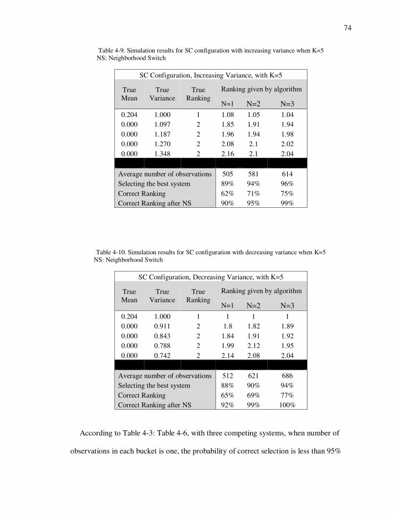
74

Table 4-9. Simulation results for SC configuration with increasing variance when K=5 NS: Neighborhood Switch

SC Configuration, Increasing Variance, with K=5

True Mean

True Variance

True Ranking


N=1 N=2 N=3

0.204 1.000 1 1.08 1.05 1.04 0.000 1.097 2 1.85 1.91 1.94 0.000 1.187 2 1.96 1.94 1.98 0.000 1.270 2 2.08 2.1 2.02 0.000 1.348 2 2.16 2.1 2.04


Table 4-10. Simulation results for SC configuration with decreasing variance when K=5 NS: Neighborhood Switch

SC Configuration, Decreasing Variance, with K=5

True Mean

True Variance

True Ranking


N=1 N=2 N=3

0.204 1.000 1 1 1 1 0.000 0.911 2 1.8 1.82 1.89 0.000 0.843 2 1.84 1.91 1.92 0.000 0.788 2 1.99 2.12 1.95 0.000 0.742 2 2.14 2.08 2.04


According to Table 4-3: Table 4-6, with three competing systems, when number of

observations in each bucket is one, the probability of correct selection is less than 95%

75

for MDM configuration with increasing and decreasing variances and more than 95% for

SC configuration with both increasing and decreasing variances. Increasing the number

of observations in each bucket, increases the probability of correct selection to more than

95% in all cases, however it generates more observations from each system. Moreover,

when there is one observation in each bucket, the probability of obtaining the correct

ranking is less than or equal to 95% in all configurations. Increasing the number of

observations in each bucket will increase the probability of obtaining the correct ranking

to more than 99%.

According to Table 4-7: Table 4-10, with five competing systems, when number of

observations in each bucket is one, the probability of correct selection is less than 95% in

all configurations. Increasing the number of observations in each bucket to N=3,

increases the probability of correct selection to more than 95% all configurations except

one configuration. It can be shown than N should be at least equal to 5 in order to obtain

95% correct selection in all configurations. Moreover, when there is one observation in

each bucket, the probability of obtaining the correct ranking is less than 85% in all

configurations. Increasing the number of observations in each bucket will increase the

probability of obtaining the correct ranking. However, with N=3, the probability of

correct ranking is still less than 85% for three configurations.

If 4g�, g�, … g(, g(=�, … , gF8 is the ranking obtained from the algorithm, then

4g�, g�, … g(=�, g(, … , gF8 is defined as the ranking after neighborhood switch. If we

perform neighborhood switch after obtaining the ranking, when K=3, then the probability

of obtaining the correct ranking after one neighborhood switch is more than 99% in all

configurations even when N=1. When K=5, after performing the neighborhood switch,

76

the probability of obtaining the correct ranking is more than 90% when N=1 and more

than or equal to 99% when N=3.

4-5. Conclusion

In this chapter we used the maximum entropy principle to present a two-stage ranking

and selection algorithm with the following contributions:

a) Relaxing the normality assumption which restricts the previous algorithms.

b) No a priori distribution is assumed.

c) Providing a ranking of systems based on the mean value of simulation outputs, and

Moreover two systems will have the same ranking if the user is indifferent among

their mean values.

At the first stage of this two-stage algorithm, based on the initial observations obtained

at the first stage, the probability distribution which maximizes uncertainty or in other

words a distribution which represents the current state of knowledge for each system is

found via using maximum entropy principle. This distribution is used to determine the

final number of observations required to rank systems in an specific confidence level and

the distribution which maximizes the uncertainty of each system is obtained based on this

final number of observations. The second stage applies directed divergence on

distributions found in the first stage to compare the systems. The efficiency of the offered

algorithm was shown by simulation experiments.

77

Chapter 5

5. Entropy-Based measure for stochastic dominance

Let � and � be two cumulative probability distributions and let ü be a positive integer.

For each distribution function $ let q#� 4e8 � $4e8 and for ) ¬ �2,3, … ¡ let q#( 4e8 �� q#(2�4$8�$ã2% . � is said to be dominated by � by stochastic dominance of order s if

q�� 4e8 � q��4e8 for all values of e with strict inequality for at least for one point e�(see

for example Levy (1992)). In the past two decades stochastic dominance has been widely

applied in different areas such as finance, risk management, and economics (see

Sriboonchita et al. (2009)).

Two possible cases for first order stochastic dominance (FSD) are illustrated in Figure

5-1. Two possible cases for FSDIn Figure 5-1.a, � and � are nondominant based on FSD

because for some values of e, �4e8 � �4e8 and for some other values �4e8 � �4e8. In

Figure 5-1.b, � dominates � based on FSD since for all values of e, �4e8 � �4e8 with

strict inequality at least for one point.

a. � and � are nondominant based on FSD b. � dominates � based on FSD

Figure 5-1. Two possible cases for FSD

Two possible cases for second order stochastic dominance (SSD) are shown Figure

5-2. In Figure 5-2.a, � dominates � based on SSD since for all values of e,

78 � �4e8�eã2% � � �4e8�eã2% with strict inequality at least for one point. In Figure 5-2.b, �

and � are nondominant based on SSD because for some values of e, � �4e8�eã2% �� 4e8�eã2% and for some other values � �4e8�eã2% � � �4e8�eã2% .

a. G dominates F based on SSD b. F and G are nondominant based on SSD

Figure 5-2. Two possible cases for SSD

Although stochastic dominance have been widely used to rank probability

distributions (see Levy (1992, 1998) for surveys on stochastic dominance), they may be

unable to determine dominance even in situations when most decision makers would

prefer one alternative over another. For example according to Leshno and Levy (2002)

suppose that two lotteries are available. Lottery X returns zero dollars with probability

0.01 and returns one million dollars with probability 0.99, while lottery Y yields one

dollar with probability 1.00. Most individuals prefer X to Y, however X does not

stochastically dominates Y according to any stochastic dominance rule of order s. This

drawback has motivated Leshno and Levy (2002) to offer stochastic dominance rules

weaker than FSD or SSD. They offered a stochastic dominance criterion that applies the

proportion of the two bounded areas, created by the crossing of the two probability

distributions, to the sum of the two areas. They named their criterion p almost first order

stochastic dominance (p-AFSD) which has been applied by several researchers such as

79

Bali et al. (2009, 2011), Tzheng et al. (2012), and Levy et al. (2010). The main advantage

of p-AFSD is the possibility for reduction of a set of nondominant alternatives.

We offer a stochastic dominance criterion weaker than FSD and SSD based on the

concept of entropy. Like p-AFSD, its advantage over the stochastic dominance criteria is

to reduce the possibility of obtaining a nondominated set of alternatives. Although, unlike

p-AFSD which compares alternatives based on surrendered areas and requires calculation

of the corresponding areas, based on the new offered criterion alternatives are compared

to a utopia and the alternative which closer to the utopia based on our definition of

closeness is chosen. The new criterion is named entropy-based stochastic dominance

(ESD). We investigate its relation with FSD, SSD, and p-AFSD. The remainder of this

chapter is organized as follows. In section 5-1, Kullback and Leibler information is

explained. Entropy-based stochastic dominance measure is presented in section 5-2. In

section 5-3 the relationship between ESD and FSD, SSD, and p-AFSD is investigated.

Finally conclusion is explained in section 5-4.

5-1. Kullback-Leibler information

Kullback-Leibler (KL) information is a measure (a ‘distance’ in an heuristic sense)

between an observed distribution, ö, and a reference distribution, c (see section 1-3 for

more details). Being denoted by Ak4ö, c8, it measures the amount of ‘information’ lost

when distribution ö is used to approximate a reference distribution, c. The analyst seeks

a distribution that its information content is as close as possible to the reference

distribution. Moreover, their measure possesses several useful properties (see Appendix

80

II) including the fact that it is always nonnegative and it is equal to zero if and only if

ö4e8 � c4e8.

Several authors have studied extensions of KL information. Asadi et al. (2004)

considered KL information for a residual distribution function with density function (4ã8�è4*8

where e r � where � is the cumulative probability distribution and �è4�8 � 1 � �4e8.

Barapour and Rad (2012) have proposed an extension of KL information for a

nonnegative random variable, called cumulative residual KL information, in terms of

survival function as follows.

wsAk4�è, sè8 � ) �è4e8 ln �è4e8�*4e8%� �e � 4�4i8 � �4+88

Where �4i8 � � �è4e8%� �e and �4+8 � � �*4e8%� �e.

Park et al. (2012) have considered another extension, called cumulative KL

information, in terms of cumulative distribution function as

wAk4�, �8 � ) �4e8 ln �4e8�4e8%� �e � 4�4i8 � �4+88

They showed that CKL is nonnegative and is equal to zero if and only if �4e8 � �4e8.

Keeping these two properties (nonnegativity and being equal to zero if and only if

�4e8 � �4e8) are the main reason that the above authors did not use � �4e8 ln �4ã8�4ã8%� �e,

as it does not keep these well-known KL information properties. If for all e, �4e8 ��4e8 then since � �4e8 ln �4ã8�4ã8%� �e is nonnegative and right continuous, when

� �4e8 ln �4ã8�4ã8%� � 0 we have �4e8 ln �4ã8�4ã8 for all e. Thus we have either �4e8 � 0 which

gives �4e8 � 0 (because 0 � �4e8 � �4e8) or we have ln �4ã8�4ã8 � 0 which means that

81

�4e8 � �4e8. Throughout this chapter we use � �4e8 ln �4ã8�4ã8%� �e as our measure for

directed divergence between � and �.

5-2. Entropy-based criterion for stochastic dominance (ESD)

We use f � � to denote hfe4f, �8 and use f , � to denote h)?4f, �8. For two

functions, ö and c, the function ö � c is called the upper envelope, or the left envelope of

ö and c, and the function ö , c is called the lower envelope, or the right envelope of ö

and c.

For a real valued function ö we use � ö to denote � ö4e8�e%2% . We use � ö- to denote

the Lebesgue integral � ö- 4e8��4e8, where � denotes the Lebesgue measure on the line.

For two functions, ö and c, the set �e: ö4e8 � c4e8¡ is denoted by �ö � c�. We will

abbreviate �ö � c� to denote ö � c when we write an integral on �ö � c�. The notation

�ö � c� is used in a similar way.

Assume that i and + are two nonnegative continuous random variables with

cumulative probability distributions � and � respectively and let k � � � � denote their

left envelope and let s � � , � denote their right envelope. Figure 5-3 shows right and

left envelopes of distributions shown in Figure 5-1.

82

a. Right and left envelopes of distributions in Figure 5-1.a b. Right and left envelopes of distributions in Figure 5-1.b

Figure 5-3. Right and left envelopes of distributions in Figure 5-1

Definition.

Let $ be a reference cumulative probability distribution.

We define � is closer to $ than � by ESD, if

.)� ln ��$�. � .)� ln ��$�. 5-1

When (5-1) is not true, we say � is not closer to $ than �.

We say � strictly dominates � by ESD if �� ln �� 0 and �� ln �� u 0.

We say � weakly dominates � by ESD when one of the following is true.

(i) � is closer to s and not closer to k than �.

(ii) � is closer to k and not closer to s than �.

We say � and � are nondominated by ESD when one of the following is true.

(i) � is closer to s and k than �.

(ii) � is closer to s and k than �.

The following two propositions are useful when two distributions are compared by ESD.

Proposition 5-1. � is closer to s than � if and only if �4� � �8 ln �� 0.

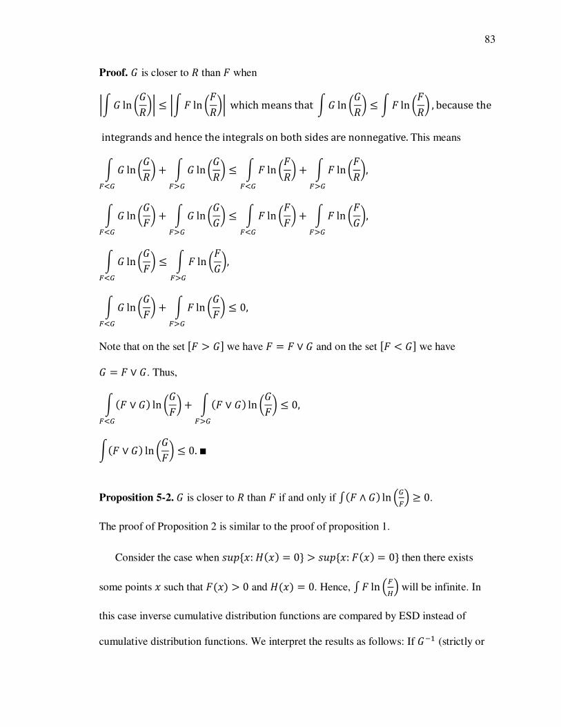
83

Proof. � is closer to s than � when

.)� ln ��s�. � .)� ln ��s�. which means that )� ln ��s� � )� ln ��s� , because the

integrands and hence the integrals on both sides are nonnegative. This means

) � ln ��s��2� ) � ln ��s��3� � ) � ln ��s��2� ) � ln ��s��3� , ) � ln ��2� ) � ln ��3� � ) � ln ��2� ) � ln ��3� , ) � ln ��2� � ) � ln ��3� , ) � ln ��2� ) � ln ��3� � 0,

Note that on the set �� we have � � � � � and on the set �� we have

� � � � �. Thus,

) 4� � �8 ln ��2� ) 4� � �8 ln ��3� � 0, )4� � �8 ln �� 0.4

Proposition 5-2. � is closer to s than � if and only if �4� , �8 ln �� r 0.

The proof of Proposition 2 is similar to the proof of proposition 1.

Consider the case when ü5'�e: $4e8 � 0¡ � ü5'�e: �4e8 � 0¡ then there exists

some points e such that �4e8 � 0 and $4e8 � 0. Hence, � � ln ��#� will be infinite. In

this case inverse cumulative distribution functions are compared by ESD instead of

cumulative distribution functions. We interpret the results as follows: If �2� (strictly or

84

weakly) dominates �2� by ESD then � dominates � and if �2� and �2� are

nondominated then � and � are nondominated as well. Three different scenarios are

illustrated in Figure 5-4.

a. � and � in scenario I b. s and k in scenario I

c. � and � in scenario II d. s and k in scenario II

e. � and � in scenario III f. s and k in scenario III

Figure 5-4. Three different scenarios when ESD is measured

In the first and third scenarios (parts a and b, and e and f of Figure 5-4),

ü5'�e: s4e8 � 0¡, ü5'�e: �4e8 � 0¡, ü5'�e: �4e8 � 0¡ , and ü5'�e: k4e8 � 0¡ are

85

equal, therefore � � ln ��, � � ln ��, � � ln ��, and � � ln �� have finite values. In

the second scenario ü5'�e: s4e8 � 0¡ � ü5'�e: �4e8 � 0¡. Thus, � � ln �� is not

defined in real numbers.

5-3. Relationship between ESD and FSD, SSD, and p-AFSD

In this section the relationship between ESD, FSD, SSD, and p-AFSD is studied.

Throughout this section assume that � and � are two continuous cumulative

distributions.

Theorem 5-1. � strictly dominates � according to ESD if and only if � dominates �

according to FSD.

Proof. If � strictly dominates � by ESD, then �� ln � ��,�� 0 and �� ln � ��,�� u 0.

This implies that � � � , � and G � � , �. Hence, � dominated � by FSD (� � �).

Inversely, if � dominated � then � � � with strict inequality at least for one point

implying that � � � , � and G � � , �. Therefore, �� ln � ��,�� 0 and

�� ln � ��,�� u 0 which means that � strictly dominates � by ESD.4

Proposition 5-3.

)� t? �� r )4� � �8 5-2

Proof. Applying Taylor series expansion to ln e at e � 1, we obtain: ln e � e � 1 �4ã2�8>�7> where 8 is a point between 1 and e. This implies that ln e � e � 1 for all e � 0

where equality holds when e � 1. Thus,

86

)� ln �� )� �� 1� � )4� � �8

Therefore,

)� ln �� )� ln �� r �)4� � �8 � )4� � �8 .4

Conjecture 5-1. If � dominates � by ESD, then � does not dominate � by SSD.

Conversely, if � dominates � by SSD, then � does not dominate � by ESD.

Assume that � dominates � by ESD and

.)� ln � �� , ��. � .)� ln � �� , ��. and .)� ln � �� . � .)� ln � �� .. )� ln � �� , �� )� ln � �� , �� and )� ln �� )� ln �� , ) � ln �� ) � ln ��

5-3

and,

) � ln �� ) � ln �� 5-4

According to proposition 5-3,

) � ln �� r )4� � �8��

5-5

) � ln �� ) 4� � �8�2� 5-6

If � dominates � based on SSD then

)4� � �8�� ) 4� � �8�2�

5-7

From (5-5), (5-6) and (5-7) we have

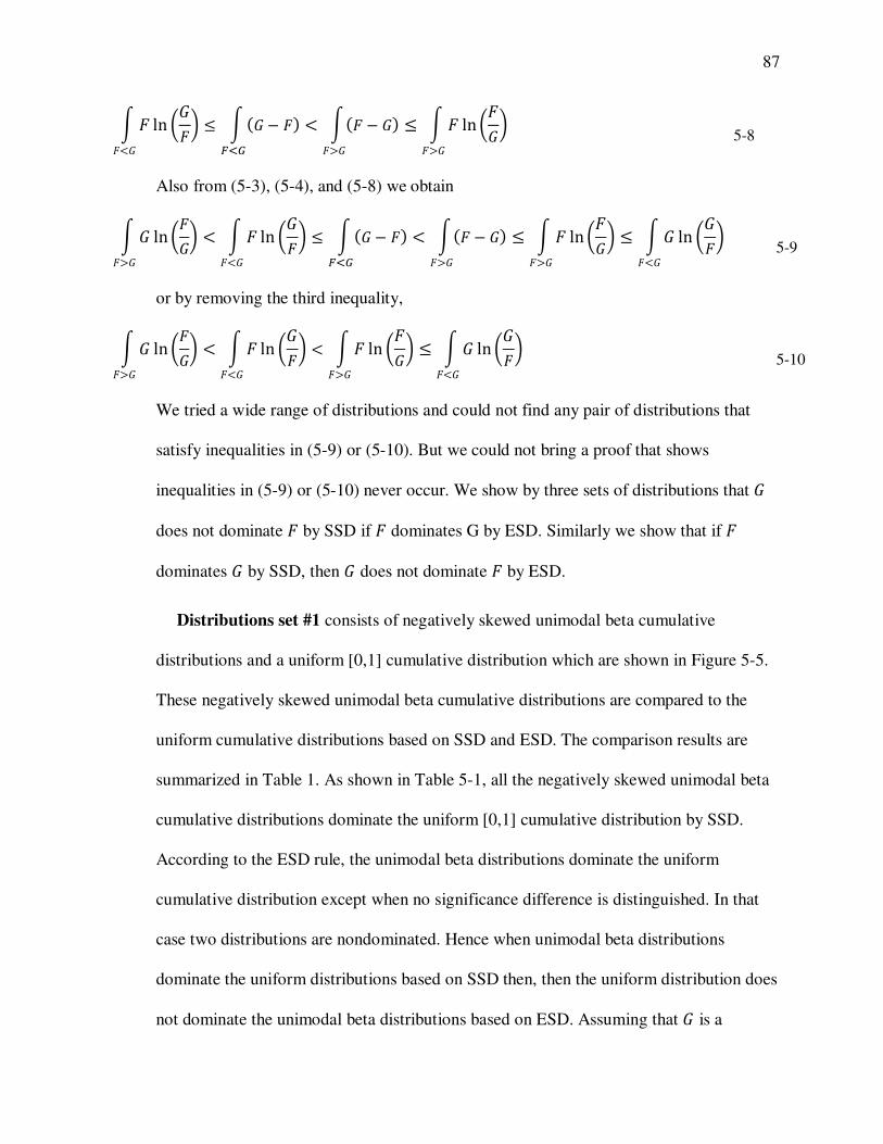
87

) � ln �� ) 4� � �8�2� � )4� � �8�� ) � ln ��

5-8

Also from (5-3), (5-4), and (5-8) we obtain

) � ln �� ) � ln �� ) 4� � �8�2� � )4� � �8�� ) � ln �� ) � ln ��

5-9

or by removing the third inequality,

) � ln �� ) � ln �� ) � ln �� ) � ln �� 5-10

We tried a wide range of distributions and could not find any pair of distributions that

satisfy inequalities in (5-9) or (5-10). But we could not bring a proof that shows

inequalities in (5-9) or (5-10) never occur. We show by three sets of distributions that �

does not dominate � by SSD if � dominates G by ESD. Similarly we show that if �

dominates � by SSD, then � does not dominate � by ESD.

Distributions set #1 consists of negatively skewed unimodal beta cumulative

distributions and a uniform [0,1] cumulative distribution which are shown in Figure 5-5.

These negatively skewed unimodal beta cumulative distributions are compared to the

uniform cumulative distributions based on SSD and ESD. The comparison results are

summarized in Table 1. As shown in Table 5-1, all the negatively skewed unimodal beta

cumulative distributions dominate the uniform [0,1] cumulative distribution by SSD.

According to the ESD rule, the unimodal beta distributions dominate the uniform

cumulative distribution except when no significance difference is distinguished. In that

case two distributions are nondominated. Hence when unimodal beta distributions

dominate the uniform distributions based on SSD then, then the uniform distribution does

not dominate the unimodal beta distributions based on ESD. Assuming that � is a

88

negatively skewed unimodal beta cumulative distribution and � is uniform [0,1]

cumulative distribution, computational results for �� ln ��, �� ln ��, �� ln ��, and �� ln �� which led to the decisions by ESD in Table 5-1 are shown in Table 5-2.

Figure 5-5. distributions set #1: negatively skewed unimodal beta and uniform [0,1] cumulative

distributions

Table 5-1. Comparison between SSD and ESD rules on distributions set #1

��q ��q ëð�f41,18 9ü ëð�f 410,38 ëð�f410,38 is dominant ëð�f410,38 is dominant ëð�f41,18 9ü ëð�f 410,48 ëð�f410,48 is dominant ëð�f410,48 is dominant ëð�f41,18 9ü ëð�f 410,58 ëð�f410,58 is dominant ëð�f410,58 is dominant ëð�f41,18 9ü ëð�f 410,68 ëð�f410,68 is dominant ëð�f410,68 is dominant ëð�f41,18 9ü ëð�f 410,78 ëð�f410,78 is dominant ëð�f410,78 is dominant ëð�f41,18 9ü ëð�f 410,88 ëð�f410,88 is dominant ëð�f410,88 is dominant ëð�f41,18 9ü ëð�f 410,98 ëð�f410,98 is dominant ëð�f410,98 is dominant ëð�f41,18 9ü ëð�f 410,9.88 ëð�f410,9.88 is dominant Nondominated set ëð�f41,18 9ü ëð�f 410,108 ëð�f410,108 is dominant Nondominated set

0 0.2 0.4 0.6 0.80

0.2

0.4

0.6

0.8

1

pbeta x 1, 1, ( )

pbeta x 10, 3, ( )

pbeta x 10, 4, ( )

pbeta x 10, 5, ( )

pbeta x 10, 6, ( )

pbeta x 10, 7, ( )

pbeta x 10, 8, ( )

pbeta x 10, 9, ( )

pbeta x 10, 9.8, ( )

pbeta x 10, 10, ( )

x

89


decisions made in Table 5-1 based on ESD, Assuming that � is a negatively skewed unimodal beta cumulative distribution and � is uniform [0,1] cumulative distribution.

�� ln �� .)� ln ��k�. .)� ln ��s�. .)� ln ��s�. ëð�f41,18 9ü ëð�f 410,38 0.158 0.002 0.002 0.428 ëð�f41,18 9ü ëð�f 410,48 0.130 0.007 0.007 0.381 ëð�f41,18 9ü ëð�f 410,58 0.108 0.015 0.017 0.313 ëð�f41,18 9ü ëð�f 410,68 0.090 0.026 0.029 0.260 ëð�f41,18 9ü ëð�f 410,78 0.076 0.037 0.044 0.218 ëð�f41,18 9ü ëð�f 410,88 0.065 0.048 0.059 0.185 ëð�f41,18 9ü ëð�f 410,98 0.058 0.051 0.073 0.164 ëð�f41,18 9ü ëð�f 410,9.88 0.052 0.065 0.084 0.148 ëð�f41,18 9ü ëð�f 410,108 0.048 0.070 0.093 0.138

Distributions set #2 consists of positively skewed bimodal beta cumulative

distributions and a uniform [0,1] cumulative distribution (Figure 5-6). The positively

skewed bimodal beta cumulative distributions are compared to the uniform cumulative

distributions based on SSD and ESD. As shown in Table 5-3, all the positively skewed

bimodal beta cumulative distributions are dominated by uniform [0,1] cumulative

distribution by SSD. According to the ESD rule, the bimodal beta distributions are

dominated by the uniform cumulative distribution except when no significance difference

is distinguished. In that case two distributions are nondominated according to ESD. Thus,

when the uniform distribution dominates the bimodal beta distributions based on SSD,

then, the bimodal beta distributions do not dominate the uniform distribution based on

ESD. Assuming that � is a positively skewed bimodal beta cumulative distribution and �

is uniform [0,1] cumulative distribution, computational results for �� ln ��, �� ln ��, �� ln ��, and �� ln �� which led to the decisions by ESD in Table 5-3

are shown in Table 5-4.

90

0 0.2 0.4 0.6 0.80

0.2

0.4

0.6

0.8

1

pbeta x 1, 1, ( )

pbeta x .8, .9, ( )

pbeta x .7, .8, ( )

pbeta x .3, .6, ( )

pbeta x .5, .7, ( )

pbeta x .4, .6, ( )

pbeta x .6, .7, ( )

pbeta x .3, .5, ( )

pbeta x .3, .4, ( )

pbeta x .3, .35, ( )

pbeta x .3, .3, ( )

x

Figure 5-6. Distributions set #2: positively skewed bimodal beta and uniform [0,1] cumulative

distributions


��q ��q ëð�f41,18 9ü ëð�f 40.8,0.98 ëð�f41,18 is dominant ëð�f41,18 is dominant ëð�f41,18 9ü ëð�f 40.7,0.88 ëð�f41,18 is dominant ëð�f41,18 is dominant ëð�f41,18 9ü ëð�f 40.3,0.68 ëð�f41,18 is dominant ëð�f41,18 is dominant ëð�f41,18 9ü ëð�f 40.5,0.78 ëð�f41,18 is dominant ëð�f41,18 is dominant ëð�f41,18 9ü ëð�f 40.4,0.68 ëð�f41,18 is dominant ëð�f41,18 is dominant ëð�f41,18 9ü ëð�f 40.6,0.78 ëð�f41,18 is dominant ëð�f41,18 is dominant ëð�f41,18 9ü ëð�f 40.3,0.58 ëð�f41,18 is dominant ëð�f41,18 is dominant ëð�f41,18 9ü ëð�f 40.3,0.48 ëð�f41,18 is dominant ëð�f41,18 is dominant ëð�f41,18 9ü ëð�f 40.3,0.358 ëð�f41,18 is dominant ëð�f41,18 is dominant ëð�f41,18 9ü ëð�f 40.3,0.38 ëð�f41,18 is dominant Nondominated set

91

Table 5-4. computational results for �� ln ��, �� ln ��, �� ln ��, and �� ln �� of decisions

made in distributions set #2 based on ESD, Assuming that � is a positively skewed bimodal beta cumulative distribution and � is uniform [0,1] cumulative distribution.

�� ln �� .)� ln ��k�. .)� ln ��s�. .)� ln ��s�. ëð�f41,18 9ü ëð�f 40.8,0.98 0.000 0.027 0.033 0.000 ëð�f41,18 9ü ëð�f 40.7,0.88 0.003 0.031 0.043 0.003 ëð�f41,18 9ü ëð�f 40.3,0.68 0.001 0.085 0.343 0.001 ëð�f41,18 9ü ëð�f 40.5,0.78 0.002 0.060 0.123 0.002 ëð�f41,18 9ü ëð�f 40.4,0.68 0.005 0.064 0.017 0.005 ëð�f41,18 9ü ëð�f 40.6,0.78 0.007 0.036 0.059 0.007 ëð�f41,18 9ü ëð�f 40.3,0.58 0.007 0.067 0.268 0.007 ëð�f41,18 9ü ëð�f 40.3,0.48 0.022 0.048 0.192 0.024 ëð�f41,18 9ü ëð�f 40.3,0.358 0.035 0.038 0.155 0.040 ëð�f41,18 9ü ëð�f 40.3,0.38 0.053 0.029 0.119 0.063

Distributions set #3 consists of positively skewed unimodal beta cumulative

distributions and a uniform [0,1] cumulative distribution (Figure 5-7). The positively

skewed unimodal beta cumulative distributions are compared to the uniform cumulative

distributions based on SSD and ESD. As shown in Table 5-5, when the positively skewed

unimodal beta cumulative distributions are dominated by uniform [0,1] cumulative

distribution by ESD, then the unimodal beta distributions does not dominate the uniform

distribution based on SSD. Assuming that � is a positively skewed unimodal beta

cumulative distribution and � is uniform [0,1] cumulative distribution, computational

results for �� ln ��, �� ln ��, �� ln ��, and �� ln �� which led to the

decisions by ESD in Table 5-5 are shown in Table 5-6.

92

Figure 5-7. Distributions set #3: positively skewed unimodal beta and uniform [0,1] cumulative

distributions


��q ��q ëð�f41,18 9ü ëð�f 43,108 Nondominated set ëð�f41,18 is dominant ëð�f41,18 9ü ëð�f 44,108 Nondominated set ëð�f41,18 is dominant ëð�f41,18 9ü ëð�f 45,108 Nondominated set ëð�f41,18 is dominant ëð�f41,18 9ü ëð�f 46,108 Nondominated set ëð�ft41,18 is dominant ëð�f41,18 9ü ëð�f 47,108 Nondominated set ëð�ft41,18 is dominant ëð�f41,18 9ü ëð�f 48,108 Nondominated set ëð�f41,18 is dominant ëð�f41,18 9ü ëð�f 49,108 Nondominated set ëð�f41,18 is dominant ëtð�f41,18 9ü ëð�f 49.5,108 Nondominated set ëð�f41,18 is dominant ëðt�f41,18 9ü ëð�f 49.8,108 Nondominated set Nondominated set

0 0.2 0.4 0.6 0.80

0.2

0.4

0.6

0.8

1

pbeta x 1, 1, ( )

pbeta x 3, 10, ( )

pbeta x 4, 10, ( )

pbeta x 5, 10, ( )

pbeta x 6, 10, ( )

pbeta x 7, 10, ( )

pbeta x 8, 10, ( )

pbeta x 9, 10, ( )

pbeta x 9.5, 10, ( )

pbeta x 9.8, 10, ( )

x

93

Table 5-6. computational results for �� ln ��, �� ln ��, �� ln ��, and �� ln �� of decisions

made in distributions set #3 based on ESD, Assuming that � is a positively skewed unimodal beta cumulative distribution and � is uniform [0,1] cumulative distribution.

�� ln �� .)� ln ��k�. .)� ln ��s�. .)� ln ��s�. ëð�f41,18 9ü ëð�f 43,108 0.001 0.175 0.398 0.003 ëð�f41,18 9ü ëð�f 44,108 0.005 0.157 0.302 0.011 ëð�f41,18 9ü ëð�f 45,108 0.010 0.138 0.236 0.025 ëð�f41,18 9ü ëð�f 46,108 0.017 0.120 0.190 0.044 ëð�f41,18 9ü ëð�f 47,108 0.025 0.105 0.155 0.066 ëð�f41,18 9ü ëð�f 48,108 0.033 0.091 0.129 0.089 ëð�f41,18 9ü ëð�f 49,108 0.040 0.098 0.124 0.113 ëð�f41,18 9ü ëð�f 49.5,108 0.044 0.102 0.120 0.117 ëð�f41,18 9ü ëð�f 49.8,108 0.047 0.072 0.096 0133

Relationship with p-AFSD

p-AFSD applies the proportion of the two bounded areas, created by the crossing of the

two probability distributions, to the sum of the two areas. In the other words p, associated

with p-AFSD is obtained by � 4�2�8:;<� 4�2�8:;< =� 4�2�8:=< . If ' is larger than a predetermined

probability, then � dominates �, otherwise they are nondominated. In case of ESD, a

probability which is shown to be too close to the probability associated with p-ASFD can

be found.

.)� ln ��s�. � )� ln � �� , �� ) � ln � �� , ��2� ) � ln � �� , ��3� �

� ) � ln ��2� ) � ln ��3� � ) � ln ��3�

� ) � ln ��3� ) � ln ��2�

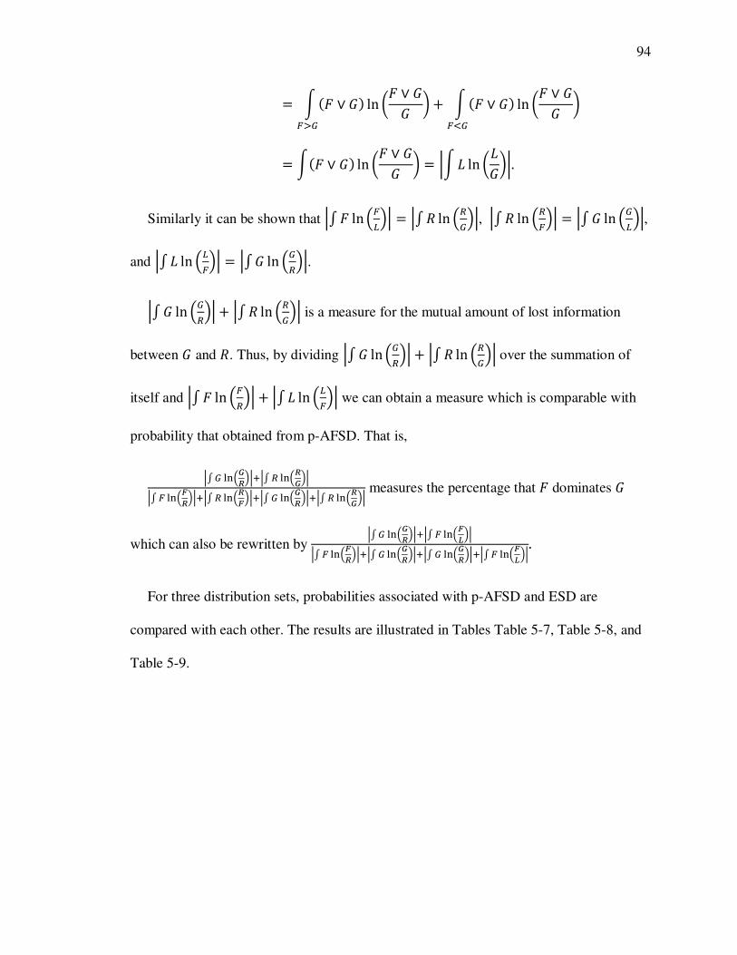
94

� ) 4� � �8 ln �� 3� ) 4� � �8 ln �� 2�

� )4� � �8 ln �� .)k ln �k��.. Similarly it can be shown that �� ln �� s ln ��, �� s ln �� ln ��,

and �� k ln �� ln ��. �� ln �� s ln �� is a measure for the mutual amount of lost information

between � and s. Thus, by dividing �� ln �� s ln �� over the summation of

itself and �� ln �� k ln �� we can obtain a measure which is comparable with

probability that obtained from p-AFSD. That is,

�� :�<>��=�� :�><�� :�:>��=�� :�>:��=�� :�<>��=�� :�><�� measures the percentage that � dominates �

which can also be rewritten by �� :�<>��=�� :�:?�� :�:>��=�� :�<>��=�� :�<>��=�� :�:?��.

For three distribution sets, probabilities associated with p-AFSD and ESD are

compared with each other. The results are illustrated in Tables Table 5-7, Table 5-8, and

Table 5-9.

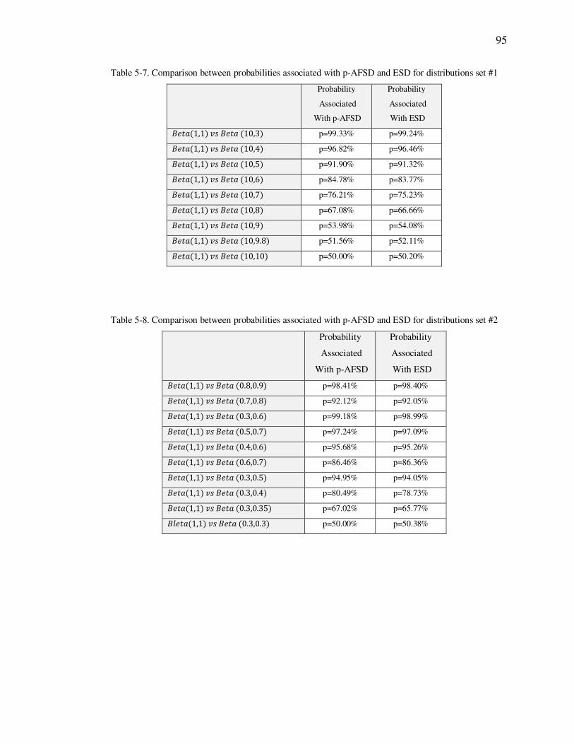
95

Table 5-7. Comparison between probabilities associated with p-AFSD and ESD for distributions set #1

Probability

Associated

With p-AFSD

Probability

Associated

With ESD ëð�f41,18 9ü ëð�f 410,38 p=99.33% p=99.24% ëð�f41,18 9ü ëð�f 410,48 p=96.82% p=96.46% ëð�f41,18 9ü ëð�f 410,58 p=91.90% p=91.32% ëð�f41,18 9ü ëð�f 410,68 p=84.78% p=83.77% ëð�f41,18 9ü ëð�f 410,78 p=76.21% p=75.23% ëð�f41,18 9ü ëð�f 410,88 p=67.08% p=66.66% ëð�f41,18 9ü ëð�f 410,98 p=53.98% p=54.08% ëð�f41,18 9ü ëð�f 410,9.88 p=51.56% p=52.11% ëð�f41,18 9ü ëð�f 410,108 p=50.00% p=50.20%


Probability

Associated

With p-AFSD

Probability

Associated

With ESD ëð�f41,18 9ü ëð�f 40.8,0.98 p=98.41% p=98.40% ëð�f41,18 9ü ëð�f 40.7,0.88 p=92.12% p=92.05% ëð�f41,18 9ü ëð�f 40.3,0.68 p=99.18% p=98.99% ëð�f41,18 9ü ëð�f 40.5,0.78 p=97.24% p=97.09% ëð�f41,18 9ü ëð�f 40.4,0.68 p=95.68% p=95.26% ëð�f41,18 9ü ëð�f 40.6,0.78 p=86.46% p=86.36% ëð�f41,18 9ü ëð�f 40.3,0.58 p=94.95% p=94.05% ëð�f41,18 9ü ëð�f 40.3,0.48 p=80.49% p=78.73% ëð�f41,18 9ü ëð�f 40.3,0.358 p=67.02% p=65.77% ëtð�f41,18 9ü ëð�f 40.3,0.38 p=50.00% p=50.38%

96


Probability

Associated

With p-AFSD

Probability

Associated

With ESD ëð�f41,18 9ü ëð�f 43,108 p=99.33% p=99.30% ëð�f41,18 9ü ëð�f 44,108 p=96.82% p=96.75% ëð�f41,18 9ü ëð� 45,108 p=91.90% p=91.83% ëð�f41,18 9ü ëð�f 46,108 p=84.78% p=84.39% ëð�f41,18 9ü ëð�f 47,108 p=76.21% p=75.45% ëð�f41,18 9ü ëð�f 48,108 p=67.08% p=66.28% ëð�f41,18 9ü ëð�f 49,108 p=60.95% p=60.67% ëð�f41,18 9ü ëð�f 49.5,108 p=53.98% p=54.07% ëð�f41,18 9ü ëð�f 49.8,108 p=51.56% p=51.87%

97

5-4. Conclusion

Using Kullback-Leibler information between two cumulative distributions, we present

an entropy-based criterion for stochastic dominance, ESD. Since our criterion is weaker

than FSD and SSD, its advantage is to reduce the possibility of obtaining a nondominated

set of alternatives. In addition, under the new stochastic dominance criterion, it is not

required to calculate the surrendered area between two distributions as it is in p-AFSD.

We investigate the relation between ESD and p-AFSD, SSD, and FSD. We show that

if a distribution is dominant based on ESD, then that distribution would not be dominated

based on SSD. Also we show that the probability associated with our new measure is too

close to the probability obtained from p-AFSD.

98

Appendix I

A simple numerical example

Suppose a discrete part manufacturing system produces two parts, part I and part II

using four work centers. Parts enter from work center 1 with the mean interarrival time of

1.25 minutes and exit from work center 4. The pickup and drop-off points are assumed to

be at the same location for each work center. Table AI.1 shows the operation sequence,

production volume percentage of each part type, and the processing time of each part

type in each work center. The vehicle speed is 100 feet per minute and the distance

between work centers is shown in Table AI.2. Loading and unloading operations are

assumed to be negligible.

Table AI-1. Operation sequences, processing times and production volume percentage of part types

Part Type Operation Sequence (processing time) Production Volume

I 1(1 minute)�2(2 minutes)�4(1 minute) %55

II 1(1 minute)�3(2 minutes)�4(2 minutes) %45

Table AI-2. The distance between work centers (feet)

Work Center 1 Work Center 2 Work Center 3 Work Center 4

Work Center 1 - 150 300 450

Work Center 2 150 - 150 300

Work Center 3 300 150 - 150

Work Center 4 450 300 150 -

Parts are being moved by a single AGV. Suppose that the vehicle is idle at work

center 2 at time �� and at this moment parts are waiting in the input queues and output

queues of each work center as illustrated in Figure AI.1.

99

Figure AI-1. Input and output queues of work centers at time �� PI @ part I; PII @ part II According to the Figure AI.1, two move requests are available for the vehicle at time ��:

1) Pickup one unit of part I from work center 2 and drop it off at work center 4 at

time �� 3.

After the completion of this move request the input and output queues of work

centers are estimated to be as Figure AI.2 :

Input queue

Output queue �¶ � �¶¶ � �¶ � �¶¶ Work Center 1 �¶ , �¶¶ , �¶¶ , �¶¶ EMPTY Work Center 2 �¶ �¶¶ Work Center 3 �¶¶ �¶ Work Center 4 �¶ , �¶¶ , �¶¶ , �¶¶

Figure AI-2. Estimated input and output queues of work centers at time �� 3 PI @ part I; PII @ part II 2) Pickup one unit of part II from work center 1 and drop it off at work center 3

at time �� 4.5. After the completion of this move request the input and

output queues of work centers are estimated to be as Figure AI.3:

Input queue

Output queue �¶ � �¶¶ � �¶ � �¶¶ � �¶¶ Work Center 1 �¶¶ �¶ Work Center 2 �¶ �¶¶ � �¶¶ Work Center 3 EMPTY

�¶¶ Work Center 4 �¶ , �¶¶ , �¶¶

100

Input queue

Output queue �¶ � �¶ � �¶¶ � �¶¶ Work Center 1 �¶ , �¶¶ , �¶¶ , �¶¶ EMPTY Work Center 2 �¶ , �¶ �¶¶ Work Center 3 �¶¶ , �¶¶ EMPTY Work Center 4 �¶ , �¶¶ , �¶¶ , �¶¶

Figure AI-3. Estimated input and output queues of work centers at time �� 4.5 PI @ part I; PII @ part II The kullback-leibler divergence measure is calculated based on each of the proposed

algorithms and the results are shown in Table AI.3:

Table AI-3. Kullback-Leibler Divergence measure calculation for each proposed algorithm

Kullback-Leibler Divergence measure

First move request Second move request

WCBA 0.9557 0.6365

OQBA 1.3768 1.3297

IOQBA 1.7329 1.6915

Since all three algorithms select the move request with the largest kullback-leibler

divergence measure, the first move request is chosen based WCBA, OQBA, and

IOQBA.

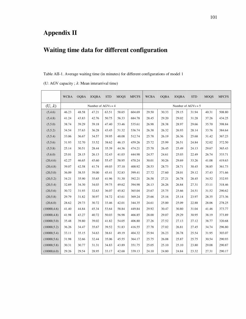
101

Appendix II

Waiting time data for different configuration

Table AII-1. Average waiting time (in minutes) for different configurations of model 1

(U: AGV capacity ; �: Mean interarrival time)

WCBA OQBA IOQBA STD MOQS MFCFS WCBA OQBA IOQBA STD MOQS MFCFS

(U, �) Number of AGVs = 4 Number of AGVs = 5

(5,4.6) 46.23 48.58 47.21 63.51 58.65 604.69 29.50 30.33 29.15 31.94 40.31 508.80

(5,4.8) 41.24 43.83 42.76 50.75 56.33 684.78 28.45 29.20 29.02 31.28 37.26 434.25

(5,5.0) 38.74 39.29 39.18 47.40 53.46 535.61 26.98 28.38 28.97 29.66 35.70 398.84

(5,5.2) 34.54 37.63 36.28 43.45 51.32 536.74 26.38 26.32 26.93 28.14 33.76 384.64

(5,5.4) 33.06 36.67 34.57 39.95 48.08 512.74 25.78 26.19 26.36 25.68 31.42 367.23

(5,5.6) 31.93 32.70 33.52 38.62 46.15 459.26 25.72 25.99 26.51 24.84 32.02 372.50

(5,5.8) 25.14 30.51 28.44 35.39 44.36 474.21 25.70 26.45 25.49 24.13 29.67 365.43

(5,6.0) 25.01 28.15 26.13 32.43 41.03 444.98 24.57 24.61 25.03 22.49 26.74 333.71

(20,4.6) 42.27 46.65 45.60 55.47 58.95 470.24 30.01 30.26 29.69 33.26 41.08 419.63

(20,4.8) 39.07 42.58 41.74 49.03 57.10 400.92 28.53 28.73 28.71 30.45 38.85 361.73

(20,5.0) 36.09 38.55 39.00 45.41 52.83 399.41 27.72 27.60 28.01 29.12 37.43 371.66

(20,5.2) 34.21 35.90 35.65 41.96 51.30 392.21 26.58 27.21 26.78 28.45 34.52 332.93

(20,5.4) 32.69 34.30 34.03 39.75 49.62 394.98 26.13 26.26 26.84 27.31 33.11 318.46

(20,5.6) 30.72 31.93 32.63 36.07 45.82 365.04 25.67 25.75 25.66 24.51 31.52 290.62

(20,5.8) 29.79 31.82 30.97 34.72 43.61 369.24 25.66 25.16 25.14 23.97 28.35 273.36

(20,6.0) 28.62 29.73 30.72 33.46 42.01 344.35 24.61 25.00 25.09 22.88 28.06 278.25

(10000,4.6) 41.40 44.84 45.34 53.64 58.84 449.84 29.92 30.47 30.80 31.04 41.46 373.77

(10000,4.8) 41.98 43.27 40.72 50.03 56.98 466.85 28.00 29.07 29.29 30.95 38.19 373.89

(10000,5.0) 35.48 39.80 39.02 41.82 54.05 406.80 27.26 27.52 27.13 27.12 38.77 320.68

(10000,5.2) 36.26 34.47 35.67 39.52 51.83 416.55 27.78 27.02 26.81 27.45 34.74 296.80

(10000,5.4) 33.11 35.15 34.63 38.61 49.19 404.32 25.94 26.23 26.78 25.54 31.95 303.07

(10000,5.6) 31.98 32.66 32.44 35.06 45.55 364.17 25.75 26.08 25.87 25.75 30.54 290.93

(10000,5.8) 30.31 30.77 31.31 34.83 43.89 351.75 25.05 25.10 25.10 23.80 29.08 290.87

(10000,6.0) 29.26 29.54 28.95 33.17 42.68 339.13 24.10 24.80 24.84 23.32 27.31 290.17

102

Table AII-2. Average waiting time (in minutes) for different configurations of model 2

(U: AGV capacity ; �: Mean interarrival time)

WCBA OQBA IOQBA STD MOQS MFCFS WCBA OQBA IOQBA STD MOQS MFCFS

(U, �) Number of AGVs=3 Number of AGVs=5

(5,4.0) 35.65 40.06 46.61 51.62 60.60 268.31 135.02 543.10 1126.02 486.86 116.50 414.62

(5,4.4) 30.69 33.30 34.56 43.87 53.84 257.35 111.97 111.97 435.67 297.54 107.00 413.79

(5,4.8) 28.59 29.28 29.77 40.06 48.64 253.99 98.37 98.37 253.82 133.94 96.77 408.69

(5,5.2) 26.80 26.83 26.91 35.80 44.40 254.73 82.18 86.68 157.22 101.65 91.94 413.70

(5,5.6) 24.96 25.09 25.27 34.00 40.12 245.63 76.52 81.06 147.63 96.55 83.06 398.91

(5,6.0) 24.40 24.99 24.90 32.31 36.27 238.89 74.81 80.72 145.48 91.74 75.11 387.97

(20,4.0) 34.56 39.89 1287.62 49.09 59.73 261.95 134.08 998.10 772.68 221.16 114.78 422.93

(20,4.4) 31.54 33.75 33.97 44.67 52.39 265.77 112.75 510.81 305.61 180.92 106.49 407.31

(20,4.8) 27.78 28.97 29.05 40.74 47.47 257.36 100.02 230.56 233.07 129.85 102.53 415.54

(20,5.2) 26.30 27.20 27.80 37.44 43.87 260.00 81.43 123.44 129.85 106.76 95.76 410.66

(20,5.6) 25.60 25.87 26.14 34.10 40.57 255.66 69.45 92.83 96.39 84.97 87.26 409.61

(20,6.0) 24.30 24.80 24.79 32.23 36.98 255.81 55.61 68.51 94.76 74.86 82.58 398.14

(10000,4.0) 39.42 44.37 35.83 49.95 60.30 261.40 144.57 326.74 325.74 851.32 117.05 495.90

(10000,4.4) 33.91 32.92 31.39 43.78 54.84 257.35 124.04 261.33 262.33 635.23 110.45 475.32

(10000,4.8) 30.11 29.99 27.82 38.62 49.29 260.02 108.27 181.17 180.07 464.52 98.91 453.62

(10000,5.2) 28.19 28.27 26.83 37.58 43.19 260.16 85.54 107.78 108.76 263.04 94.58 406.70

(10000,5.6) 25.92 26.90 24.88 34.47 40.68 260.62 67.84 98.34 97.40 135.00 90.67 430.07

(10000,6.0) 24.26 25.47 24.18 32.99 37.09 254.01 55.05 74.34 75.44 77.37 84.39 409.70

103

Appendix III

Proof of theorems 4.1-4.3

Proof of Theorem 4.1.

By the central limit theorem it can be shown that √?4fè � á8~B40, ∑ 4�|2�è8>�|¼<72� 8. On

the other hand '(�B � ð2Ñ«2Ñ<ã|2� � 1. This function is continuous and has first partial

derivative with respect to the component á at á � fè. Hence, according the multivariate

delta method:

√?4��è � ��B8~��B40, ï² ∑ 4�|2�è8>�|¼<72� ï8 where ï( � ßC{|�DCB .BG�è E'(�BEá � E'(�BE��

E��Eá E'(�BE��E��Eá AIII-1

By replacing '(�B � ð2Ñ«2Ñ<ã|2� � 1 in the first and second constraints of model (I) we

will have:

3Íe2Ñ«2Ñ<ã|2� � 1Ïê(G� � 1 F 4ë 18ðÑ«=� � 3ße2Ñ<ã| ßê

(G� AIII-2

3 e(Íe2Ñ«2Ñ<ã|2� � 1Ïê(G� � á F ðÑ«=� � ∑ e( ßeß2Ñ<ã| ß ßê(G�á ∑ e(ê(G� AIII-3

By combining equations (AIII-2) and (AIII-3) we will get:

á � 4ë 18 ∑ e(ð2Ñ<ã|ê(G�∑ ð2Ñ<ã|ê(G� � 3 e(ê

(G� AIII-4

� Calculating CÑ<CB : from equation (AIII-4)

104

EáE�� 4ë 18Í∑ e(�ð2Ñ<ã|ê(G� ÏÍ∑ ð2Ñ<ã|ê(G� Ï 4ë 18Í∑ e(ð2Ñ<ã|ê(G� Ï�4∑ ð2Ñ<ã|ê(G� 8� AIII-5

Hence:

E��Eá � Í∑ ð2Ñ<ã|ê(G� Ï��4ë 184∑ e(�ð2Ñ<ã|ê(G� 84∑ ð2Ñ<ã|ê(G� 8 4ë 184∑ e(ð2Ñ<ã|ê(G� 8� AIII-6

� Calculating CÑ«CB : from equation (AIII-2)

4ë 18ðÑ« E��E�� 3ße(eß2Ñ<ã|2�ß ßê(G� F E��E�� ∑ ße(eß2Ñ<ã|2Ñ«2�ß ßê(G� ë 1

F E��E�� fè � ∑ e(ê(G�ë 1 AIII-7

E��Eá � E��E��E��Eá

� � fè ∑ e(ê(G�4ë 18� � Í∑ ð2Ñ<ã|ê(G� Ï�4� ∑ e(�ð2Ñ<ã|ê(G� 84∑ ð2Ñ<ã|ê(G� 8 4∑ e(ð2Ñ<ã|ê(G� 8� AIII-8

� Calculating C{�DCÑ< and

C{|�DCÑ« : Since '(�B � ð2Ñ«2Ñ<ã|2� � 1, we have:

E'(�BE�� e(ð2Ñ«2Ñ<ã|2� AIII-9

E'(�BE�� ð2Ñ«2Ñ<ã|2� AIII-10

105

Therefore by replacing CÑ<CB ,

CÑ«CB , C{|�DCÑ< and

C{|�DCÑ« equations (AIII-6), (AIII-8), (AIII-9) and

(AIII-10) into equation (AIII-1), we obtain:

ï( � � 4ë 182�Í∑ ð2Ñ<ã|ê(G� Ï�4� ∑ e(�ð2Ñ<ã|ê(G� 84∑ ð2Ñ<ã|ê(G� 8 4∑ e(ð2Ñ<ã|ê(G� 8��. ð2Ñ«2Ñ<ã|2� ´fè ∑ e(ê(G�ë 1 � e(À

4

AIII-11

106


Since √?4��è � ��B8 G� ��B40, Σ8, Using Taylor series expansion we obtain:

�4��è8 � �4��B8 §²4��è � ��B8 s Where § � 4§�, §�, … , §ê8 are the values

given above and s H 0 fü ? H∞. Thus it follows that √?Í�4��è8 � �4��B8ÏG� B40, â�8 and estimated divergence variance, â� � §Σ§�. Hence �4��è8 J $� �v â/√?

is an approximate 10041 � ~8% confidence interval for �4��B8 where $� �v is the upper

~ 2v percentage point from the normal distribution.

4

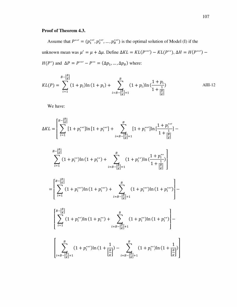
107


Assume that �� 4'��, '��, … , 'ê��8 is the optimal solution of Model (I) if the

unknown mean was á� � á ∆á. Define ∆Ak � Ak4��8 � Ak4��8, ∆$ � $4��8 �$4��8 and ∆� � �� 4∆'�, … ,∆'ê8 where:

Ak4�8 � 3 41 '(8lnê2ñòMó(G� 41 '(8 3 41 '(8lnê

(Gê2ñòMó=�41 '(1 �ñòMó

8 AIII-12

We have:

ΔAk � NOOP 3 �1 '(��lnê2ñòMó

(G� �1 '(�� 3 �1 '(��lnê(Gê2ñòMó=�

�1 '(��1 �ñòMó� ß �

ß 3 41 '(��8lnê2ñòMó(G� 41 '(��8 3 41 '(��8lnê

(Gê2ñòMó=�41 '(��1 �ñòMó

8QRRS

� NOOP 3 41 '(��8lnê2ñòMó

(G� 41 '(��8 3 41 '(��8lnê(Gê2ñòMó=�

41 '(��8QRRS �

NOOP 3 41 '(��8lnê2ñòMó

(G� 41 '(��8 3 41 '(��8lnê(Gê2ñòMó=�

41 '(��8QRRS �

T 3 41 '(��8lnê(Gê2ñòMó=�

41 1ñêFó8 � 3 41 '(��8lnê(Gê2ñòMó=�

41 1ñêFó8U

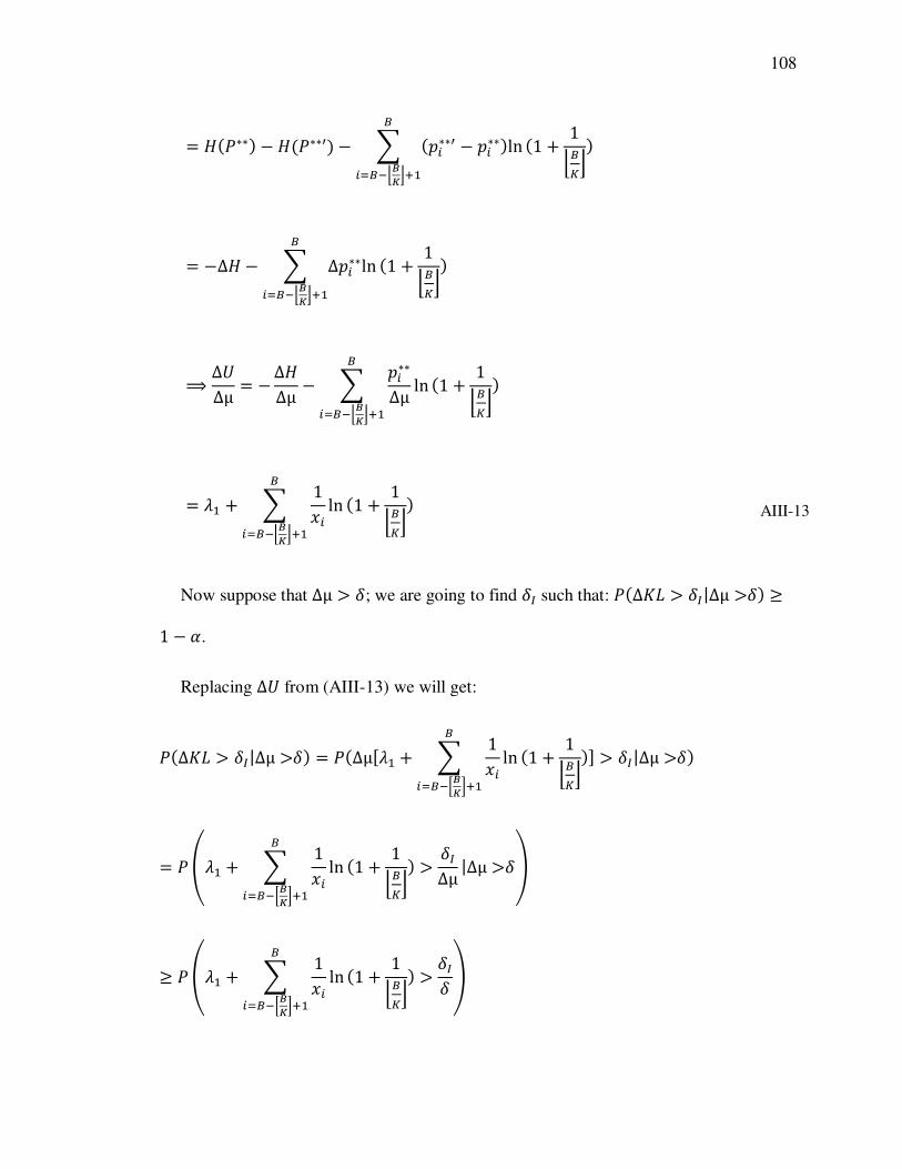
108

� $4��8 � $4��8 � 3 4ß'(�� ß � '(��8lnê(Gê2ñòMó=�

41 1ñêFó8

� �∆$ � 3 ßß∆'(�� ßßlnê(Gê2ñòMó=�

41 1ñêFó8

F Δ�∆µ � �∆$∆µ � 3 '(��∆µ lnê(Gê2ñòMó=�

41 1ñêFó8

� �� 3 1e( lnê(Gê2ñòMó=�

41 1ñêFó8 AIII-13

Now suppose that ∆µ � �; we are going to find �¶ such that: �4∆Ak � �¶|∆µ �ß�8 r1 � ~.

Replacing ∆� from (AIII-13) we will get:

�4∆Ak � �¶|∆µ �ß�8 � �4∆µ�� 3 1e( lnê(Gê2WòMX=�

41 1ñêFó8� � �¶|∆µ �ß�8

� � ýß�� 3 1e( lnê(Gê2WòMX=�

41 1ñêFó8ß � �¶∆µ |∆µ �ß�þ

r � ýß�� 3 1e( lnê(Gê2WòMX=�

41 1ñêFó8ß � �¶�þ

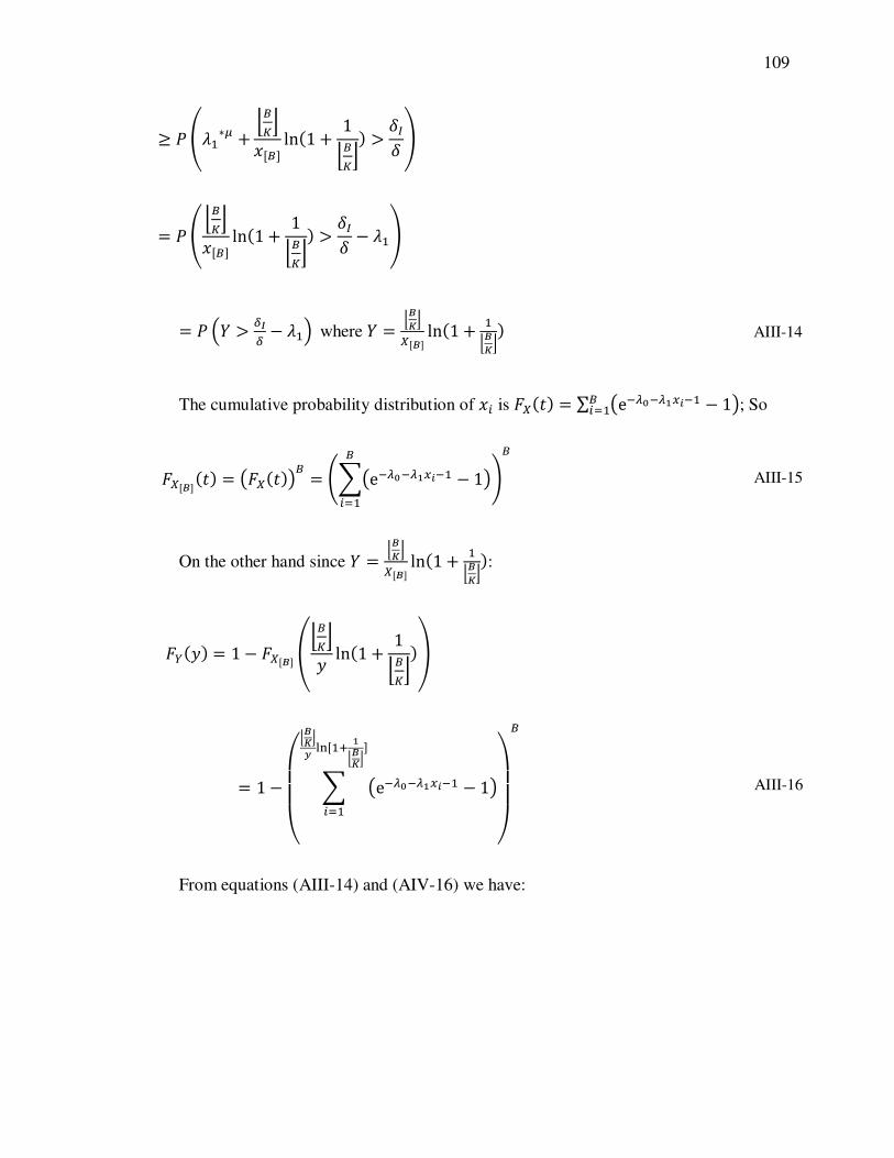
109

r ��ß��B ß ñêFóe�ê� ln41 1ñêFó8 � �¶� �

� �� ñêFóe�ê� ln41 1ñêFó8 � �¶� � ��

� � �+ � �� where + � ñòMóY�ò� ln41 �ñòMó8 AIII-14

The cumulative probability distribution of e( is �Y4�8 � ∑ Íe2Ñ«2Ñ<ã|2� � 1Ïê(G� ; So

�Y�ò�4�8 � Í�Y4�8Ïê � �3Íe2Ñ«2Ñ<ã|2� � 1Ïê(G� �ê

AIII-15

On the other hand since + � ñòMóY�ò� ln41 �ñòMó8:

��48 � 1 � �Y�ò� ýñêFó ln41 1ñêFó8þ

� 1 �� 3 Íe2Ñ«2Ñ<ã|2� � 1Ï

ñòMó �:��= <ñòMó�(G� �

��ê

AIII-16

From equations (AIII-14) and (AIV-16) we have:

110

1 � �� ¶� � �� 3 Íe2Ñ«2Ñ<ã|2� � 1Ï

ñòMóZ�Z [\<�:��= <ñòMó�

(G� ��

êr 1 � ~

F �¶� � �� r ��2�41 � ~8 AIII-17

So we will choose �¶ such that it satisfies (AIV-17).

111

References

Abbas., A.E. (2006). Entropy. Wiley Encyclopedia of Biomedical Engineering, John

Wiley & Sons, Inc.

Ahmadi-Javid, A. (2012). Entropic Value-at-Risk: A New Coherent Risk Measure,

Journal Optimization Theory and Applications,155: 1105–1123.

Asadi, M., Ebrahimi, N., Hamedani, G.G., Soofi, E.S. (2004). Maximum dynamic

entropy models. Journal of Applied Probability, 41: 379–390.

Aczel, J.D., Daroczy, Z. (1975), On Measures of Information and Their Generalizations.

Academic Press, New York.

Bali, T.G., Brown, S.J., Demirtas, K.O. (2011). Investing in stock market anomalies.

Working paper. Georgetown University, Washington, DC.

Bali, T.G., Demirtas, K.O., Levy, H., Wolf, A. (2009). Bonds versus stocks: Investors’

age and risk taking. Journal of Monetary Economics, 56(6): 817–830.

Barapour, S., Rad, A.H. (2012). Testing goodness-of-fit for exponential distribution

based on cumulative residual entropy. Communications in Statistics: Theory and

Methods, 41: 1387-1396.

Bartholdi, J.J., Platzman, L.K. (1989). Decentralized control of automated guided

vehicles on a simple loop. IIE Transactions, 21(1), 76-81.

Bechhofer, R.E., Santner, T. J. (1995). Goldsman, D. M., Design and Analysis of

experiments for Statistical Selection. Screening, and Multiple Comparisions, John

Wiley & Sons, Inc., NewYork.

112

Becker, C., Scholl, A. (2006). A survey on problems and methods in generalized

assembly line balancing. European Journal of Operational Research, 168: 694-715.

Bera, A.K., Park, S.Y. (2005). Optimal portfolio diversification using the maximum

entropy principle. In: Proceedings of the Second Conference on Recent

Developments in the Theory, Method, and Applications of Information and Entropy

Econometrics, The American University Washington, DC, USA.

Bera, A.K., Park, S.Y. (2008). Optimal portfolio diversification using the maximum

entropy principle. Econometric Review, 27: 484–512.

Bhattacharyya, R., Ahmed Hossain, S., Kar, S. (2013). Fuzzy cross-entropy, mean,

variance, skewness models for portfolio selection. Journal of King Saud University-

Computer and Information Sciences, Article in press.

Boltzmann, L. (1871a). Analytischer Beweis des zweiten Haubtsatzes der mechanischen

Wärmetheorie aus den Sätzen über das Gleichgewicht der lebendigen Kraft. Wiener

Berichte, 63, 712–732. In Boltzmann (1909), Volume 1, Paper 20. Cited in Uffink

(2004)

Boltzmann, L. (1871b). Einige allgemeine Sätze über wärmegleichgewicht. Wiener

Berichte, 63, 679–711. In Boltzmann (1909), Volume 1, Paper 19. Cited in Uffink

(2004)

Boltzmann, L. (1871c). Über das Wärmegleichgewicht zwischen mehratomigen

Gasmolekülen. Wiener Berichte, 63, 397–418. In Boltzmann (1909), Volume 1, Paper

18. Cited in Uffink (2004)

Bozer, Y.A., Yen, C.K. (1996). Intelligent dispatching rules for trip-based material

handling systems. Journal of Manufacturing Systems, 15(4): 226-239.

113

Calinescu, A., Efstathiou, J., Schirn, J., Bermejo, J. (1998). Applying and assessing two

methods for measuring complexity in manufacturing. Journal of the Operational

Research Society, 49: 723-733.

Chang, A.Y., Whitehouse, D.J., Chang, S.L., Hsieh, Y.C. (2001). An approach to the

measurement of single-machine flexibility. International Journal of Production

Research, 39 (8): 1589-1601.

Chang, A.Y. (2004). On the measurement of labor flexibility. Proceeding of the IEEE

International Engineering Management Conference IEMC-2004, October, Singapore:

18-22.

Chang, A.Y. (2007). On the measurement of routing flexibility: A multiple attribute

approach. International Journal of Production Economics, 109: 122-136.

Chang, A.Y. (2009). An attribute approach to the measurement of machine-group

flexibility. European Journal of Operational Research, 194: 774-786.

Chen, H.C., Chen. C.H., Yucesan, E. (2000). Computing efforts allocation for ordinal

optimization and discrete event simulation. IEEE Transactions on Automatic Control,

45: 960-964.

Chengli, Z., Yan, Y. (2012). Coherent Risk Measure Based on Relative Entropy. Applied

Mathematics & Information Sciences, 6(2): 233-238.

Chick, S. E., Inoue, K. (2001). New two-stage and sequential procedures for selecting the

best simulated system. Operations Research, 49 (5): 732-743.

Csiszer, I. (1972). A Class of Measures of Informativity of Observation Channels,

Periodica Mathematica Hungarica, 2: 191-213.

114

Deshmukh, A.V. (1993). Complexity and chaos in manufacturing systems, PhD Thesis,

Purdue University, USA.

Deshmukh, A.V., Talavage, J.J., Barash, M.M. (1998). Complexity in manufacturing

systems. Part 1: Analysis of static complexity. IIE Transactions, 30(4): 35-44.

Egbelu, P.J., Tanchoco, J.M.A. (1984). Characterization of automatic guided vehicle

dispatching rules. International Journal of Production Research, 22(3): 359-374.

Föllmer, H., Knispel, T. (2011). Entropic risk measures: coherence vs. convexity, model

ambiguity, and robust large deviations. stochastic and dynamics, 11(333).

Frizelle, G., Woodcock, E., (1995). Measuring complexity as an aid to developing

operational strategy. International Journal of Operation and Production Management,

15(5): 26-39.

Frizelle, G. (1996). An entropic measurement of complexity in manufacturing operations

Internal Report of the Institute for Manufacturing. Cambridge University, Cambridge,

UK.

Frizelle, G., Suhov, Y.M. (2001). An entropic measurement of queueing behavior in a

class of manufacturing operations. Proceedings of the Royal Society, London, 457:

1579–1601.

Fujimoto, H., Ahmed, A., Iida, Y., Hanai, M. (2003). Assembly process design for

managing manufacturing complexities because of product varieties. International

Journal of Flexible Manufacturing Systems, 15: 283-307.

Gaur, D.R., Gupta, A., Krishnamurti, R. (2003). An approximation algorithm for

scheduling vehicles on a path with release and handling times. Information

Processing Letters, 86: 87-91.

115

Gibbs, J. W. (1902). Elementary Principles in Statistical Mechanics, Developed with

Especial Reference to the Rational Foundations of Thermodynamics. C. Scribner’s

sons, New York.

Guan, X. and Dai, X. (2009). Deadlock-free multi-attribute dispatching method for AGV

systems. International Journal of Advanced Manufacturing Technology, 45 (5–6),

603–615.

Gupta, S.S., Miescke, K.J. (1994). Bayesian look ahead one stage sampling allocations

for selecting the largest normal mean. Statistical Papers, 35: 169-177.

Gupta, S. S., Miescke, K.J. (1996). Bayesian look ahead one-stage sampling allocations

for selection of the best population. Journal of Statistical Planning and Inference, 54:

229-244.

Havrada, J. H., Charvat, F. (1967). Quantification methods of classification processes:

Concepts of structural entropy. Kybernetika, 3: 30-35.

Ho, Y.C., Chein, S.H. (2006). A simulation study on the performance of task

determination rules and delivery dispatching rules for multi-load AGVs. International

Journal of Production Research, 44(20): 4193-4222.

Hong, L.J., Nelson, B.L. (2005). The tradeoff between sampling and switching: New

sequential procedures for indifference-zone selection. IIE Transactions, 37: 623-634.

Hong, L.J., Nelson, B.L. (2007). Selecting the best system when systems are revealed

sequentially. IIE Transactions, 39: 723-734.

Huang, X. (2008). Mean-entropy models for fuzzy portfolio selection. IEEE Transactions

on Fuzzy Systems, 16: 1096-1101.

116

Hwang, H., Kim, S.H. (1998). Development of dispatching rules for automated guided

vehicles, journal of manufacturing systems. journal of manufacturing systems, 17(2):

137-143.

Jana, P., Roy, T.K., Mazumder, S.K. (2009). Multi-objective possibilistic model for

portfolio selection with transaction cost. Journal of Computational and Applied

Mathematics, 1: 188–196.

Jaynes, E. T. (1957a). Information theory and statistical mechanics. Physical review,

106(4): 620-630.

Jaynes, E. T. (1957b). Information theory and statistical mechanics II, Physical review,

108(2): 171-190.

Jeong, B.H., Randhawa, S.U. (2001). A multi-attribute dispatching rule for automated

guided vehicle systems. International Journal of Production Research, 39(13): 2817-

2832.

Jones, B.L., Zitikis, R. (2007). Risk measures, distortion parameters, and their empirical

estimation. Insurance: Mathematics and Economics, 41: 279–297.

Kapur, J. N., Kesavan, H. K. (1992). Entropy optimization principles with applications.

Academic press, Inc., NewYork.

Kapur, J. N. (1993). Maximum Entropy Models in Science and Engineering. John Wiley

& Sons, Inc., NewYork.

Kim, S.H., Nelson, B. L. (2001). A fully sequential procedure for indifference-zone

selection in simulation. ACM Transactions on Modeling and Computer Simulation,

11: 251-273.

117

Kim, J., Klein, C. M. (1996). AGV dispatching. International Journal of Production

Research, 34(1): 95-110.

Kim, C.W., Tanchoco, J.M.A. (1991). Conflict-free shortest-time bidirectional AGV

routing. International Journal of Production Research, 29(12): 2377-2391.

Kim, C.W., Tanchoco, J.M.A., Koo, P.H. (1999). AGV dispatching based on workload

balancing. International Journal of Production Research, 37 (17): 4053-4066.

Kim, S.H., Hwang, H. (1999). An adaptive dispatching algorithm for automated guided

vehicles based on an evolutionary process. International Journal of Production

Economics, 60–61: 465-472.

Kim, K.S., Chung, B.D., Park, Y.S. (2004). Minimum empty distance dispatching rules

for a single loop-single vehicle AGV system, International Journal of Industrial

Engineering, 11(3): 252-260.

Kullback, S. (1959). Information Theory and Statistics, Wiley, New York.

Kullback, S., Leibler, R. A. (1951). On information and sufficiency. Annals of

mathematical statistics, 22(1): 79-86.

Kumar, V. (1987). Entropic measurement of manufacturing flexibility. International

Journal of Production Research, 25 (7): 957-966.

Kumar, V. (1988). Measurement of loading and operations flexibility in flexible

manufacturing systems: An information-theoretic approach. Annals of Operations

Research, 15: 65-80.

Leshno, M., Levy, H. (2002). Preferred by “all” and preferred by “most” decision

makers: Almost stochastic dominance. Management Science, 48(8):1074–1085.

118

Levy, H. (1992). Stochastic dominance and expected utility: Survey and analysis.

Management Science, 38(4): 555–593.

Levy, H. (1998). Stochastic Dominance: Investment Decision Making Under

Uncertainty. Kluwer Academic, Boston.

Levy, H., Leshno, M., Leibovitch, B. (2010). Economically relevant preferences for all

observed epsilon. Annals of Operations Research. 176(1): 153–178.

Lexa, M. (2004). Useful Facts About the Kullback-Leibler Discrimination Distance. Rice

Univ. Houston, TX, Tech. Rep.

Mandelbaum, M. (1990). Flexibility and decision making. European Journal of

Operational Research, 44: 17–27.

Martinez-Olvera, C. (2008). Entropy as an assessment tool of supply chain information

sharing. European Journal of Operations Research, 185, 405-417.

Mathai, A.M., Rathie, P.N. (1975), Basic Concepts in Information Theory and Statistics.

Wiley Eastern Ltd., New Delhi.

Mukhopadhyay, S.K., Midha, S., Krishna, V.M. (1992). A heuristic procedure for loading

problems in manufacturing systems. International Journal of Production Research, 30,

2213-2228.

Naso, D., Turchiano, B. (2005). Multi-criteria Meta-Heuristics for AGV Dispatching

Control Based on Computational Intelligence. IEEE Transaction Systems, Man, and

Cybernetics-PART B: Cybernetics, 35(2): 208-226.

119

Nelson, B. L., Swann, J., Goldsman, D., Song, W. (2001). Simple procedures for

selecting the best simulated system when the number of alternatives in large.

Operations Research, 49: 950-963.

Nelson, B. L., Staum, J. (2006). Control variates for screening, selection, and estimation

of the best. ACM transactions on Modeling and Computer Simulation, 16: 52-57.

Nishi, T., Shimatani, K., Inuiguchi, M. (2009). Decomposition of Petri nets and

Lagrangian relaxation for solving routing problems for AGVs. International Journal

of Production Research, 47(14), 3957-3977.

Nishi, T., Ando, M., Konishi, M. (2005). Experimental studies on a local rescheduling

procedure for dynamic routing of autonomous decentralized AGV systems. Robotics

and Computer-Integrated Manufacturing, 22(2): 154-165.

Olivella, J., Corominas, A., Pastor, R. (2010). An entropy-based measurement of working

time flexibility. European Journal of Operational Research, 200: 253-260.

Park, S., Rao, M., Shin, D.W. (2012). On cumulative residual Kullback-Leibler

information. Statistics and Probability Letters, 82: 2025–2032.

Pereira, J., Paulre, B. (2001). Flexibility in manufacturing systems: A relational and a

dynamic approach, European Journal of Operational Research, 130: 70–82.

Pichitlamken, J., Nelson, B. L., Hong. L. (2006). A sequential procedure for

neighborhood selection-of-the-best in optimization via simulation, European Journal

of Operational Research, 173 283-298.

Piplani, R., Wetjens, D. (2007). Evaluation of entropy-based dispatching in flexible

manufacturing systems. European Journal of Operational Research, 176: 317-331.

120

Rao, H.A., Gu, P. (1994). Flexibility in cellular manufacturing systems: An entropic

measure. Proceedings of the 10th ISPE/IFAC International Conference on

CAD/CAM, Robotics and Factories of the Future, 411-416.

Rinott, Y. (1978). On two-stage selection procedures and related probability inequalities.

Communications in Statistics, A7: 799-811.

Rödder, W., Gartner, I.R., Rudolph, S. (2010). An entropy-driven expert system shell

applied to portfolio selection. Expert Systems with Applications, 37(12): 7509–7520.

Sabuncuoglu, I. (1998). A study of scheduling rules of flexible manufacturing systems: A

simulation approach. International Journal of Production Research, 36(2): 527-546.

Scuricini, G.B. (1987). Complexity in large technological systems, Measures of

Complexity. Rome, Italy, 83–101.

Sethi, A.K., Sethi, S.P. (1990). Flexibility in manufacturing: A survey. International

Journal of Flexible Manufacturing Systems, 2: 289-328.

Shannon, C. E. (1948). A mathematical theory of communication, Bell System Technical

Journal, 27:379-423, 623-656.

Sharma, B. D., Mittal, D. P. (1975). New non-additive measures of entropy for discrete

probability distributions. Journal of mathematical sciences, 10:28-40.

Shuiabi, E., Thomson, V., Bhuiyan, N. (2005). Entropy as a measure of operational

flexibility. European Journal of Operational Research, 165: 696-707.

Sivadasan, S., Efstathiou, J., Frizelle, G., Shirazi, R., Calinescu,A. (2002). An

information-theoretic methodology for measuring the operational complexity of

supplier–customer systems, International Journal of Operations and Production

Management, 22(1): 80-102.

121

Sivadasan, S., Efstathiou, J., Calinescu, A., Huaccho, H. L. (2006). Advances on

measuring the operational complexity of supplier– customer systems. European

Journal of Operations Research, 171(1): 208-226.

Sivadasan, S., Smart, J., Huaccho, H. L., Calinescu, A. (2010). Operational complexity

and supplier–customer integration: case study insights and complexity rebound.

Journal of the Operational Research Society, 61: 1709 -1718.

Sriboonchita, S., Wong, W.K., Dhompongsa, S., Nguyen, H.T. (2009). Stochastic

Dominance and Applications to Finance, Risk and Economics. Chapman and

Hall/CRC, Taylor &Francis Group, Boca Raton, FL, USA.

Stecke, K.E. (1983). Formulation and solution of nonlinear integer production planning

problems for flexible manufacturing systems, Management Science, 29: 273-288.

Tan, K.K., Tang, K.Z. (2001). Vehicle dispatching system based on Taguchi-tuned fuzzy

rules. European Journal of Operational Research, 128: 545–557.

Tsai, S.C., Nelson, B.L., Staum, J. (2009). Combined screening and selection of the best

with control variates. In: Advancing the Frontiers of simulation: A Festschrift in

Honor of George S. Fishman, Kluwer, 263-289.

Tzeng, L.Y., Huang, R.J., Shih, P.T. (2012) Revisiting Almost Second-Degree Stochastic

Dominance. Management Science, Articles in Advance, 1-5.

Qina, Z., Lia, X., Ji, X. (2009). Portfolio selection based on fuzzy cross-entropy. Journal

of Computational and Applied Mathematics, 228: 139-149.

122

Veeravalli, B., Rajesh, G., Viswanadham, N. (2002). Design and analysis of optimal

material distribution policies in flexible manufacturing systems using a single AGV.

International Journal of Production Research, 40(12): 2937–2954.

Wu, Y., Frizelle, G., Efstathiou, J. (2007). A study on the cost of operational complexity

in customer–supplier systems. International Journal of Production Economy, 106(1):

217–229.

Wu, Z.W., Song, X.F., Xu, Y.Y., Liu, K. (2009). A note on a minimax rule for portfolio

selection and equilibrium price system. Applied Mathematics and Computation, 208:

49–57.

Yamashita, H. (2001). Analysis of dispatching rules of AGV systems with multiple

vehicles. IIE Transactions, 33: 889–895.

Yang, J., Qiu, W. (2005). A measure of risk and a decision-making model based on

expected utility and entropy. European Journal of Operational Research, 164: 792–

799.

Yao, D. D. (1985). Material and information flows in flexible manufacturing systems.

Material Flows, 2: 143–149.

Yao, D. D., Pei, F.F. (1990). Flexible parts routing in manufacturing systems. IIE

Transactions, 1990, 22: 48–55.

Yu, S. B., Efstathiou, J. (2006). Complexity in rework cells: Theory, analysis and

comparison. Journal of the Operational Research Society, 57(5): 593–602.

Zaremba, M.B., Obuchowicz, A., Banaszak, Z.A., Jedrzejek, K.J. (1997). A max-algebra

approach to the robust distributed control of repetitive AGV systems. International

Journal of Production Research, 35(10): 2667–2687.

123

Zhang, W., Liu, Y.J., Wei-Jun Xu. (2012). A possibilistic mean-semivariance-entropy

model for multi-period portfolio selection with transaction costs. European Journal of

Operational Research, 222: 341–349.

entropy applications in industrial engineering

Documents