entropy and diversity - arxiv
TRANSCRIPT
This material has been published by Cambridge University Press as Entropy and Diversity: The Axiomatic Approach by Tom Leinster.This version is free to view and download for personal use only. Not for re-distribution, re-sale or use in derivative works.
Paperback: https://www.cambridge.org/9781108965576. Hardback: https://www.cambridge.org/9781108832700.© Tom Leinster 2020
Entropy and diversityThe axiomatic approach
T O M L E I N S T E RUniversity of Edinburgh
The printed version of this book is available in paperback or hardback.This arXiv version appears by agreement with Cambridge University Press.
I thank CUP for offering this arrangement.
arX
iv:2
012.
0211
3v2
[q-
bio.
PE]
22
Jun
2021

This material has been published by Cambridge University Press as Entropy and Diversity: The Axiomatic Approach by Tom Leinster.This version is free to view and download for personal use only. Not for re-distribution, re-sale or use in derivative works.
Paperback: https://www.cambridge.org/9781108965576. Hardback: https://www.cambridge.org/9781108832700.© Tom Leinster 2020
Much of this book was written in Catalonia duringthe turbulent years since 2017. I dedicate it to all
those in Catalonia who struggle for theirdemocratic rights.
This material has been published by Cambridge University Press as Entropy and Diversity: The Axiomatic Approach by Tom Leinster.This version is free to view and download for personal use only. Not for re-distribution, re-sale or use in derivative works.
Paperback: https://www.cambridge.org/9781108965576. Hardback: https://www.cambridge.org/9781108832700.© Tom Leinster 2020
Contents
Interdependence of chapters page ivNote to the reader vAcknowledgements viIntroduction 1
1 Fundamental functional equations 151.1 Cauchy’s equation 161.2 Logarithmic sequences 231.3 The q-logarithm 28
2 Shannon entropy 322.1 Probability distributions on finite sets 332.2 Definition and properties of Shannon entropy 392.3 Entropy in terms of coding 442.4 Entropy in terms of diversity 522.5 The chain rule characterizes entropy 58
3 Relative entropy 623.1 Definition and properties of relative entropy 633.2 Relative entropy in terms of coding 663.3 Relative entropy in terms of diversity 703.4 Relative entropy in measure theory, geometry and
statistics 743.5 Characterization of relative entropy 85
4 Deformations of Shannon entropy 914.1 q-logarithmic entropies 924.2 Power means 1004.3 Renyi entropies and Hill numbers 1114.4 Properties of the Hill numbers 1194.5 Characterization of the Hill number of a given order 127
i

This material has been published by Cambridge University Press as Entropy and Diversity: The Axiomatic Approach by Tom Leinster.This version is free to view and download for personal use only. Not for re-distribution, re-sale or use in derivative works.
Paperback: https://www.cambridge.org/9781108965576. Hardback: https://www.cambridge.org/9781108832700.© Tom Leinster 2020
ii Contents
5 Means 1335.1 Quasiarithmetic means 1355.2 Unweighted means 1425.3 Strictly increasing homogeneous means 1495.4 Increasing homogeneous means 1555.5 Weighted means 162
6 Species similarity and magnitude 1696.1 The importance of species similarity 1716.2 Properties of the similarity-sensitive diversity measures 1826.3 Maximizing diversity 1926.4 Introduction to magnitude 2066.5 Magnitude in geometry and analysis 217
7 Value 2247.1 Introduction to value 2267.2 Value and relative entropy 2367.3 Characterization of value 2407.4 Total characterization of the Hill numbers 245
8 Mutual information and metacommunities 2578.1 Joint entropy, conditional entropy and mutual information 2588.2 Diversity measures for subcommunities 2698.3 Diversity measures for metacommunities 2738.4 Properties of the metacommunity measures 2838.5 All entropy is relative 2948.6 Beyond 299
9 Probabilistic methods 3039.1 Moment generating functions 3049.2 Large deviations and convex duality 3079.3 Multiplicative characterization of the p-norms 3159.4 Multiplicative characterization of the power means 322
10 Information loss 32910.1 Measure-preserving maps 33010.2 Characterization of information loss 336
11 Entropy modulo a prime 34311.1 Fermat quotients and the definition of entropy 34411.2 Characterizations of entropy and information loss 35211.3 The residues of real entropy 35511.4 Polynomial approach 359

This material has been published by Cambridge University Press as Entropy and Diversity: The Axiomatic Approach by Tom Leinster.This version is free to view and download for personal use only. Not for re-distribution, re-sale or use in derivative works.
Paperback: https://www.cambridge.org/9781108965576. Hardback: https://www.cambridge.org/9781108832700.© Tom Leinster 2020
Contents iii
12 The categorical origins of entropy 36812.1 Operads and their algebras 36912.2 Categorical algebras and internal algebras 37712.3 Entropy as an internal algebra 38412.4 The universal internal algebra 385
Appendix A Proofs of background facts 395A.1 Forms of the chain rule for entropy 395A.2 The expected number of species in a random sample 398A.3 The diversity profile determines the distribution 399A.4 Affine functions 401A.5 Diversity of integer orders 402A.6 The maximum entropy of a coupling 403A.7 Convex duality 406A.8 Cumulant generating functions are convex 407A.9 Functions on a finite field 408
Appendix B Summary of conditions 409References 412Index of notation 431Index 433

This material has been published by Cambridge University Press as Entropy and Diversity: The Axiomatic Approach by Tom Leinster.This version is free to view and download for personal use only. Not for re-distribution, re-sale or use in derivative works.
Paperback: https://www.cambridge.org/9781108965576. Hardback: https://www.cambridge.org/9781108832700.© Tom Leinster 2020
Interdependence of chapters
A dotted line indicates that one chapter is helpful, but not essential, for another.
1. Fundamental
functional equations
2. Shannon entropy
3. Relative entropy
4. Deformations of
Shannon entropy
5. Means
7. Value 9. Probabilistic methods
6. Species similarity
and magnitude
10. Information loss
11. Entropy
modulo a prime
12. The categorical
origins of entropy
8. Mutual information
and metacommunities
iv

This material has been published by Cambridge University Press as Entropy and Diversity: The Axiomatic Approach by Tom Leinster.This version is free to view and download for personal use only. Not for re-distribution, re-sale or use in derivative works.
Paperback: https://www.cambridge.org/9781108965576. Hardback: https://www.cambridge.org/9781108832700.© Tom Leinster 2020
Note to the reader
This book began life as a seminar course on functional equations at the Univer-sity of Edinburgh in 2017, motivated by recent research on the quantificationof biological diversity. The course attracted not only mathematicians in sub-jects from stochastic analysis to algebraic topology, but also participants fromphysics and biology. In response, I did everything I could to minimize themathematical prerequisites.
I have tried here to retain the broad accessibility of the course. At the sametime, I have not censored myself from including the many fruitful connectionswith more advanced parts of mathematics.
These two opposing forces have been reconciled by confining the more ad-vanced material to separate chapters or sections that can easily be omitted.Chapter 9 requires some probability theory, Chapter 11 some abstract algebra,and Chapter 12 some category theory, while Sections 3.4, 6.4 and 6.5 also callon parts of geometry, analysis and statistics. However, the core narrative threadrequires no more mathematics than a first course in rigorous (ε-δ) analysis.Readers with this background are promised that they are equipped to followall the main ideas and results. The parts just listed, and any remarks that referto more specialized knowledge, can safely be omitted.
Moreover, those who regard themselves as wholly ‘pure’ mathematicianswill find no barriers here. Although much of this book is about the diversity ofecological systems, no knowledge of ecology is needed. Similarly, the infor-mation theory that we use is introduced from the ground up.
In the middle parts of the book, many conditions on means and diversitymeasures are defined: homogeneity, consistency, symmetry, etc. Appendix Bcontains a summary of this terminology for easy reference. There is also anindex of notation.
v
This material has been published by Cambridge University Press as Entropy and Diversity: The Axiomatic Approach by Tom Leinster.This version is free to view and download for personal use only. Not for re-distribution, re-sale or use in derivative works.
Paperback: https://www.cambridge.org/9781108965576. Hardback: https://www.cambridge.org/9781108832700.© Tom Leinster 2020
Acknowledgements
Many people have given me encouragement and the benefit of their insight,wisdom, and expertise. I am especially grateful to John Baez, Jim Borger, TonyCarbery, Jose Figueroa-O’Farrill, Tobias Fritz, Herbert Gangl, Heiko Gimper-lein, Dan Haydon, Richard Hepworth, Andre Joyal, Joachim Kock, BarbaraMable, Louise Matthews, Richard Reeve, Emily Roff, Mike Shulman, ToddTrimble, Simon Willerton, and Xılıng Zhang, as well as Roger Astley at CUP.
My heartfelt thanks go to Christina Cobbold and Mark Meckes, not onlyfor many thought-provoking mathematical conversations over the years, butalso for taking the time to read drafts of this text, which their perceptive andknowledgeable comments helped to improve.
I thank all of those involved in the original functional equations seminarcourse in Edinburgh for their good humour and friendly participation. Interac-tions during those seminars were formative for my understanding. So too weremany conversations at The n-Category Cafe, a research blog that has been in-valuable for my learning of new mathematics.
I owe a great deal to the Boyd Orr Centre for Population and EcosystemHealth, an interdisciplinary research centre at the University of Glasgow, ofwhich I have been happy to have been a member since 2010. It is a model of theinterdisciplinary spirit: welcoming, collaborative, informal, and scientificallyambitious. Warm thanks to all who foster that positive atmosphere.
This work was supported at different times by an EPSRC Advanced Re-search Fellowship, a BBSRC FLIP award (BB/P004210/1), and a LeverhulmeTrust Research Fellowship. Critical research advances were made during a2012 programme on the Mathematics of Biodiversity at the Centre de Re-cerca Matematica (CRM) in Barcelona, which was supported by the CRM,a Spanish government grant, and a BBSRC International Workshop Grant; Iwas also supported personally there by the Carnegie Trust for the Universitiesof Scotland. Finally, I thank the Department of Mathematics at the Universitat
vi

This material has been published by Cambridge University Press as Entropy and Diversity: The Axiomatic Approach by Tom Leinster.This version is free to view and download for personal use only. Not for re-distribution, re-sale or use in derivative works.
Paperback: https://www.cambridge.org/9781108965576. Hardback: https://www.cambridge.org/9781108832700.© Tom Leinster 2020
Acknowledgements vii
Autonoma de Barcelona for their hospitality during part of the writing of thisbook.
Some parts of Section 6.3 first appeared in Leinster and Meckes [219], andare reproduced with the second author’s permission.

This material has been published by Cambridge University Press as Entropy and Diversity: The Axiomatic Approach by Tom Leinster.This version is free to view and download for personal use only. Not for re-distribution, re-sale or use in derivative works.
Paperback: https://www.cambridge.org/9781108965576. Hardback: https://www.cambridge.org/9781108832700.© Tom Leinster 2020
Introduction
This book was born of research in category theory, brought to life by the on-going vigorous debate on how to quantify biological diversity, given strengthby information theory, and fed by the ancient field of functional equations. Itapplies the power of the axiomatic method to a biological problem of pressingconcern, but it also presents new advances in ‘pure’ mathematics that stand intheir own right, independently of any application.
The starting point is the connection between diversity and entropy. We willdiscover:
• how Shannon entropy, originally defined for communications engineering,can also be understood through biological diversity (Chapter 2);
• how deformations of Shannon entropy express a spectrum of viewpoints onthe meaning of biodiversity (Chapter 4);
• how these deformations provably provide the only reasonable abundance-based measures of diversity (Chapter 7);
• how to derive such results from characterization theorems for the powermeans, of which we prove several, some new (Chapters 5 and 9).
Complementing the classical techniques of these proofs is a large-scale cate-gorical programme, which has produced both new mathematics and new mea-sures of diversity now used in scientific applications. For example, we willfind:
• that many invariants of size from across the breadth of mathematics (includ-ing cardinality, volume, surface area, fractional dimension, and both topo-logical and algebraic notions of Euler characteristic) arise from one singleinvariant, defined in the wide generality of enriched categories (Chapter 6);
• a way of measuring diversity that reflects not only the varying abundances of
1

This material has been published by Cambridge University Press as Entropy and Diversity: The Axiomatic Approach by Tom Leinster.This version is free to view and download for personal use only. Not for re-distribution, re-sale or use in derivative works.
Paperback: https://www.cambridge.org/9781108965576. Hardback: https://www.cambridge.org/9781108832700.© Tom Leinster 2020
2 Introduction
species (as is traditional), but also the varying similarilities between them,or, more generally, any notion of the values of the species (Chapters 6 and 7);
• that these diversity measures belong to the extended family of measures ofsize (Chapter 6);
• a ‘best of all possible worlds’: an abundance distribution on any given setof species that maximizes diversity from an infinite number of viewpointssimultaneously (Chapter 6);
• an extension of Shannon entropy from its classical context of finite sets todistributions on a metric space or a graph (Chapter 6), obtained by translat-ing the similarity-sensitive diversity measures into the language of entropy.
Shannon entropy is a fundamental concept of information theory, but informa-tion theory contains many riches besides. We will mine them, discovering:
• how the concept of relative entropy not only touches subjects from Bayesianinference to coding theory to Riemannian geometry, but also provides a wayof quantifying local diversity within a larger context (Chapter 3);
• quantitative methods for identifying particularly unusual or atypical parts ofan ecological community (Chapter 8, drawing on work of Reeve et al. [290]).
The main narrative thread is modest in its mathematical prerequisites. But wealso take advantage of some more specialized bodies of knowledge (large devi-ation theory, the theory of operads, and the theory of finite fields), establishing:
• how probability theory can be used to solve functional equations (Chapter 9,following work of Aubrun and Nechita [20]);
• a streamlined characterization of information loss, as a natural consequenceof categorical and operadic thinking (Chapters 10 and 12);
• that the concept of entropy is (provably) inescapable even in the pure-mathematical heartlands of category theory, algebra and topology, quite sep-arately from its importance in scientific applications (Chapter 12);
• the right definition of entropy for probability distributions whose ‘probabil-ities’ are elements of the ring Z/pZ of integers modulo a prime p (Chap-ter 11, drawing on work of Kontsevich [193]).
The question of how to quantify diversity is far more mathematically profoundthan is generally appreciated. This book makes the case that the theory of di-versity measurement is fertile soil for new mathematics, just as much as theneighbouring but far more thoroughly worked field of information theory.
∗ ∗ ∗

This material has been published by Cambridge University Press as Entropy and Diversity: The Axiomatic Approach by Tom Leinster.This version is free to view and download for personal use only. Not for re-distribution, re-sale or use in derivative works.
Paperback: https://www.cambridge.org/9781108965576. Hardback: https://www.cambridge.org/9781108832700.© Tom Leinster 2020
Introduction 3
What is the problem of quantifying diversity? Briefly, it is to take a bio-logical community and extract from it a numerical measure of its ‘diversity’(whatever that should mean). This task is certainly beset with practical prob-lems: for instance, field ecologists recording woodland animals will probablyobserve the noisy, the brightly-coloured and the gregarious more frequentlythan the quiet, the camouflaged and the shy. There are also statistical difficul-ties: if a survey of one community finds 10 different species in a sample of 50individuals, and a survey of another finds 18 different species in a sample of100, which is more diverse?
However, we will not be concerned with either the practical or the statisticaldifficulties. Instead, we will focus on a fundamental conceptual problem: inan ideal world where we have complete, perfect data, how can we quantifydiversity in a meaningful and logical way?
In both the news media and the scientific literature, the most common mean-ing given to the word ‘diversity’ (or ‘biodiversity’) is simply the number ofspecies present. Certainly this is an important quantity. However, it is not al-ways very informative. For instance, the number of species of great ape on theplanet is 8 (Example 4.3.8), but 99.99% of all great apes belong to just onespecies: us. In terms of global ecology, it is arguably more accurate to say thatthere is effectively only one species of great ape.
An example illustrates the spectrum of possible interpretations of the con-cept of diversity. Consider two bird communities:
A B
In community A, there are four species, but the majority of individuals belongto a single dominant species. Community B contains the first three species inequal abundance, but the fourth is absent. Which community, A or B, is morediverse?
One viewpoint is that the presence of species is what matters. Rare speciescount for as much as common ones: every species is precious. From this view-
This material has been published by Cambridge University Press as Entropy and Diversity: The Axiomatic Approach by Tom Leinster.This version is free to view and download for personal use only. Not for re-distribution, re-sale or use in derivative works.
Paperback: https://www.cambridge.org/9781108965576. Hardback: https://www.cambridge.org/9781108832700.© Tom Leinster 2020
4 Introduction
point, community A is more diverse, simply because more species are present.The abundances of species are irrelevant; presence or absence is all that mat-ters.
But there is an opposing viewpoint that prioritizes the balance of commu-nities. Common species are important; they are the ones that exert the mostinfluence on the community. Community A has a single very common species,which has largely outcompeted the others, whereas community B has threecommon species, evenly balanced. From this viewpoint, community B is morediverse.
These two viewpoints are the two ends of a continuum. More precisely, thereis a continuous one-parameter family (Dq)q∈[0,∞] of diversity measures encod-ing this spectrum of viewpoints. Low values of q attach high importance torare species; for example, D0 measures community A as more diverse thancommunity B. When q is high, Dq is most strongly influenced by the balanceof more common species; thus, D∞ judges B to be more diverse. No singleviewpoint is right or wrong. Different scientists adopt different viewpoints (thatis, different values of q) for different purposes, as the literature amply attests(Examples 4.3.5).
Long ago, it was realized that the concept of diversity is closely related tothe concept of entropy. Entropy appears in dozens of guises across dozens ofbranches of science, of which thermodynamics is probably the most famous.(The introduction to Chapter 2 gives a long but highly incomplete list.) Themost simple incarnation is Shannon entropy, which is a real number associatedwith any probability distribution on a finite set. It is, in fact, the logarithm ofthe diversity measure D1. Most often, Shannon entropy is explained and un-derstood through the theory of coding; indeed, we provide such an explanationhere. But the diversity interpretation provides a new perspective.
For example, the diversity measures Dq, known in ecology as the Hill num-bers, are the exponentials of what information theorists know as the Renyientropies. From the very beginning of information theory, an important rolehas been played by characterization theorems: results stating that any measure(of information, say) satisfying a list of desirable properties must be of a par-ticular form (a scalar multiple of Shannon entropy, say). But what counts asa desirable property depends on one’s perspective. We will prove that the Hillnumbers Dq are, in a precise sense, the only measures of diversity with certainnatural properties (Theorem 7.4.3). This theorem translates into a new charac-terization of the Renyi entropies, but it is not one that necessarily would havebeen thought of from a purely information-theoretic perspective.
However, something is missing. In the real world, diversity is understood asinvolving not only the number and abundances of the species, but also how dif-
This material has been published by Cambridge University Press as Entropy and Diversity: The Axiomatic Approach by Tom Leinster.This version is free to view and download for personal use only. Not for re-distribution, re-sale or use in derivative works.
Paperback: https://www.cambridge.org/9781108965576. Hardback: https://www.cambridge.org/9781108832700.© Tom Leinster 2020
Introduction 5
ferent they are. (For example, this affects conservation policy; see the OECDquotation on p. 169.) We describe the remedy in Chapter 6, defining a fam-ily of diversity measures that take account of the varying similarity betweenspecies, while still incorporating the spectrum of viewpoints discussed above.This definition unifies into one family a large number of the diversity measuresproposed and used in the ecological and genetics literature.
This family of diversity measures first appeared in a paper in Ecology [218],but it can also be understood and motivated from a purely mathematical per-spective. The classical Renyi entropies are a family of real numbers assignedto any probability distribution on a finite set. By factoring in the differences ordistances between points (species), we extend this to a family of real numbersassigned to any probability distribution on a finite metric space. In the extremecase where d(x, y) = ∞ for all distinct points x and y, we recover the Renyientropies. In this way, the similarity-sensitive diversity measures extend thedefinition of Renyi entropy from sets to metric spaces.
Different values of the viewpoint parameter q ∈ [0,∞] produce differentjudgements on which of two distributions is the more diverse. But it turns outthat for any metric space (or in biological terms, any set of species), there isa single distribution that maximizes diversity from all viewpoints simultane-ously. For a generic finite metric space, this maximizing distribution is unique.Thus, almost every finite metric space carries a canonical probability distribu-tion (not usually uniform). The maximum diversity itself is also independentof q, and is therefore a numerical invariant of metric spaces. This invariant hasgeometric significance in its own right (Section 6.5).
We go further. One might wish to evaluate an ecological community in a waythat takes into account some notion of the values of the species (such as phylo-genetic distinctiveness). Again, there is a sensible family of measures that doesthis job, extending not only the similarity-sensitive diversity measures just de-scribed, but also further measures already existing in the ecological literature.The word ‘sensible’ can be made precise: as soon as we subject an abstractmeasure of the value of a community to some basic logical requirements, itis forced to belong to a certain one-parameter family (σq) (Theorem 7.3.4),which are essentially the Renyi relative entropies.
Information theory also helps us to analyse the diversity of metacommuni-ties, that is, ecological communities made up of a number of smaller communi-ties such as geographical regions. The established notions of relative entropy,conditional entropy and mutual information provide meaningful measures ofthe structure of a metacommunity (Chapter 8). But we will do more than sim-ply translate information theory into ecological language. For example, thenew characterization of the Renyi entropies mentioned above is a byproduct of
This material has been published by Cambridge University Press as Entropy and Diversity: The Axiomatic Approach by Tom Leinster.This version is free to view and download for personal use only. Not for re-distribution, re-sale or use in derivative works.
Paperback: https://www.cambridge.org/9781108965576. Hardback: https://www.cambridge.org/9781108832700.© Tom Leinster 2020
6 Introduction
the characterization theorem for measures of ecological value. In this way, thetheory of diversity gives back to information theory.
∗ ∗ ∗
The scientific importance of biological diversity goes far beyond the obvi-ous setting of conservation of animals and plants. Certainly such conservationefforts are important, and the need for meaningful measures of diversity iswell-appreciated in that context. For example, Vane-Wright et al. [339] wrotethirty years ago of the ‘agony of choice’ in conservation of flora and fauna, andemphasized how crucial it is to use the right diversity measures.
But most life is microscopic. Nee [259] argued in 2004 that
[w]e are still at the very beginning of a golden age of biodiversity dis-covery, driven largely by the advances in molecular biology and a newopen-mindedness about where life might be found,
and that
all of the marvels in biodiversity’s new bestiary are invisible.
Even excluding exotic new discoveries of microscopic life, two recent lines ofresearch illustrate important uses of diversity measures at the microbial level.
First, the extensive use of antimicrobial drugs on animals unfortunateenough to be born into the modern meat industry is commonly held to be acause of antimicrobial resistance in pathogens affecting humans. However, a2012 study of Mather et al. [244] suggests that the causality may be morecomplex. By analysing the diversity of antimicrobial resistance in Salmonellataken from animal populations on the one hand, and from human populationson the other, the authors concluded that the animal population is ‘unlikely to bethe major source of resistance’ for humans, and that ‘current policy emphasison restricting antimicrobial use in domestic animals may be overly simplis-tic’. The diversity measures used in this analysis were the Hill numbers Dq
mentioned above and central to this book.Second, the increasing problem of obesity in humans has prompted re-
search into causes and treatments, and there is evidence of a negative cor-relation between obesity and diversity of the gut microbiome (Turnbaugh etal. [331, 332]). Almost all traditional measures of diversity rely on a divisionof organisms into species or other taxonomic groups, but in this case, only afraction of the microbial species concerned have been isolated and classifiedtaxonomically. Researchers in this field therefore use DNA sequence data, ap-plying sophisticated but somewhat arbitrary clustering algorithms to create ar-tificial species-like groups (‘operational taxonomic units’). On the other hand,

This material has been published by Cambridge University Press as Entropy and Diversity: The Axiomatic Approach by Tom Leinster.This version is free to view and download for personal use only. Not for re-distribution, re-sale or use in derivative works.
Paperback: https://www.cambridge.org/9781108965576. Hardback: https://www.cambridge.org/9781108832700.© Tom Leinster 2020
Introduction 7
the similarity-sensitive diversity measures mentioned above and introduced inChapter 6 can be applied directly to the sequence data, bypassing the cluster-ing step and producing a measure of genetic diversity. A test case was carriedout in Leinster and Cobbold [218] (Example 4), with results that supported theconclusions of Turnbaugh et al.
Despite the wide variety of uses of diversity measures in biology, none of themathematics presented in this text is intrinsically biological. Indeed, the math-ematics of diversity was being developed as early as 1912 by the economistCorrado Gini [116] (best known for the Gini coefficient of disparity of wealth),and by the statistician Udny Yule in the 1940s for the analysis of lexical di-versity in literature [358]. Some of the diversity measures most common inecology have recently been used to analyse the ethnic and sociological diver-sity of judges (Barton and Moran [30]), and the similarity-sensitive diversitymeasures that are the subject of Chapter 6 have been used not only in multipleecological contexts (as listed after Example 6.1.8), but also in non-biologicalapplications such as computer network security (Wang et al. [344]).
In mathematical terms, simple diversity measures such as the Hill num-bers are invariants of a probability distribution on a finite set. The similarity-sensitive diversity measures are defined for any probability distribution on a fi-nite set with an assigned degree of similarity between each pair of points. (Thisincludes any finite metric space or graph.) The value measures are defined forany finite set equipped with a probability distribution and an assignment of anonnegative value to each element. The metacommunity measures are definedfor any probability distribution on the cartesian product of a pair of finite sets.Much of this text is written using ecological terminology, but the mathematicsis entirely general.
∗ ∗ ∗
This work grew out of a general category-theoretic study of size. In manyparts of mathematics, there is a canonical notion of the size of the objectsof study: sets have cardinality, vector spaces have dimension, subsets of Eu-clidean space have volume, topological spaces have Euler characteristic, andso on. Typically, such measures of size satisfy analogues of the elementaryinclusion-exclusion and multiplicativity formulas for counting finite sets:
|X ∪ Y | = |X| + |Y | − |X ∩ Y |,
|X × Y | = |X| · |Y |.
(The interpretation of Euler characteristic as the topological analogue of car-dinality is not as well known as it should be; this is an insight of Schanuel on

This material has been published by Cambridge University Press as Entropy and Diversity: The Axiomatic Approach by Tom Leinster.This version is free to view and download for personal use only. Not for re-distribution, re-sale or use in derivative works.
Paperback: https://www.cambridge.org/9781108965576. Hardback: https://www.cambridge.org/9781108832700.© Tom Leinster 2020
8 Introduction
which we elaborate in Section 6.4.) From a categorical perspective, it is naturalto seek a single invariant unifying all of these measures of size.
Some unification is achieved by defining a notion of size for categoriesthemselves, called magnitude or Euler characteristic. (Finiteness hypothesesare required, but will not be mentioned in this overview.) This definition al-ready brings together several established invariants of size [208]: cardinalityof sets, and the various notions of Euler characteristic for partially orderedsets, topological spaces, and even orbifolds (whose Euler characteristics are ingeneral not integers). The theory of magnitude of categories is closely relatedto the theory of Mobius–Rota inversion for partially ordered sets [298, 213].
But the decisive, unifying step is the generalization of the definition of mag-nitude from categories to the wider class of enriched categories [214], whichincludes not only categories themselves, but also metric spaces, graphs, andthe additive categories that are a staple of homological algebra.
The definition of the magnitude of an enriched category unifies still more es-tablished invariants of size. For example, in the representation theory of asso-ciative algebras, one frequently considers the indecomposable projective mod-ules, which form an additive category. The magnitude of that additive categoryturns out to be the Euler form of a certain canonical module, defined as analternating sum of dimensions of Ext groups (equation (6.20)). Magnitude forenriched categories can also be realized as the Euler characteristic of a certainHochschild-like homology theory of enriched categories, in the same sensethat the Jones polynomial for knots is the Euler characteristic of Khovanovhomology [187]. This was established in recent work led by Shulman [222],building on the case of magnitude homology for graphs previously developedby Hepworth and Willerton [142].
Since any metric space can be regarded as an enriched category, the generaldefinition of the magnitude of an enriched category gives, in particular, a def-inition of the magnitude |X| ∈ R of a metric space X. Unlike the other specialcases just mentioned, this invariant is essentially new.
Recent, increasingly sophisticated, work in analysis has connected magni-tude with classical invariants of geometric measure. For example, for a com-pact subset X ⊆ Rn satisfying certain regularity conditions, if one is given themagnitude of all of the rescalings tX of X (for t > 0), then one can recover:
• the Minkowski dimension of X (one of the principal notions of fractional di-mension), a result proved by Meckes using results in potential theory (The-orem 6.5.9);
• the volume of X, a result proved by Barcelo and Carbery using PDE methods(Theorem 6.5.6);
This material has been published by Cambridge University Press as Entropy and Diversity: The Axiomatic Approach by Tom Leinster.This version is free to view and download for personal use only. Not for re-distribution, re-sale or use in derivative works.
Paperback: https://www.cambridge.org/9781108965576. Hardback: https://www.cambridge.org/9781108832700.© Tom Leinster 2020
Introduction 9
• the surface area of X, a result proved by Gimperlein and Goffeng usingglobal analysis (or more specifically, tools for computing heat trace asymp-totics; Theorem 6.5.8).
Gimperlein and Goffeng also proved an asymptotic inclusion-exclusion prin-ciple:
|t(X ∪ Y)| + |t(X ∩ Y)| − |tX| − |tY | → 0
as t → ∞, for sufficiently regular X,Y ⊆ Rn (Section 6.5). This is anothermanifestation of the cardinality-like nature of magnitude.
We have seen that every finite metric space X has an unambiguous maximumdiversity Dmax(X) ∈ R, defined in terms of the similarity-sensitive diversitymeasures (p. 5). We have also seen that X has a magnitude |X| ∈ R. Thesetwo real numbers are not in general equal (ultimately because probabilities orspecies abundances are forbidden to be negative), but they are closely related.Indeed, Dmax(X) is always equal to the magnitude of some subspace of X,and in important families of cases is equal to the magnitude of X itself. So,magnitude is closely related to maximum diversity. Indeed, this relationshipwas exploited by Meckes to prove the result on Minkowski dimension.
There is a historical surprise. Although this author arrived at the definitionof the magnitude of a metric space by the route of enriched category theory, ithad already arisen in earlier work on the quantification of biodiversity. In 1994,the environmental scientists Andrew Solow and Stephen Polasky carried out aprobabilistic analysis of the benefits of high biodiversity ([316], Section 4), andisolated a particular quantity that they called the ‘effective number of species’.They did not investigate it mathematically, merely remarking mildly that it ‘hassome appealing properties’. It is exactly our magnitude.
∗ ∗ ∗
Ecologists began to propose quantitative definitions of biological diversity inthe mid-twentieth century [311, 348], setting in motion more than sixty yearsof heated debate, with dozens of further proposed diversity measures, hun-dreds of scholarly papers, at least one book devoted to the subject [238], andconsequently, for some, despair (expressed as early as 1971 in a famously-titled paper of Hurlbert [148]). Meanwhile, parallel debates were taking placein genetics and other disciplines.
The connections between diversity measurement on the one hand, and infor-mation theory and category theory on the other, are fruitful for both mathemat-ics and biology. But any measure of biological diversity must be justifiable inpurely biological terms, rather than by borrowing authority from information

This material has been published by Cambridge University Press as Entropy and Diversity: The Axiomatic Approach by Tom Leinster.This version is free to view and download for personal use only. Not for re-distribution, re-sale or use in derivative works.
Paperback: https://www.cambridge.org/9781108965576. Hardback: https://www.cambridge.org/9781108832700.© Tom Leinster 2020
10 Introduction
theory, category theory, or any other field. The ecologist E. C. Pielou warnedagainst attaching ecological significance to diversity measures for anythingother than ecological reasons:
It should not be (but it is) necessary to emphasize that the object of calcu-lating indices of diversity is to solve, not to create, problems. The indicesare merely numbers, useful in some circumstances but not in all. [. . . ]Indices should be calculated for the light (not the shadow) they cast ongenuine ecological problems.
([280], p. 293).In a series of incisive papers beginning in 2006, the conservationist and
botanist Lou Jost insisted that whatever diversity measures one uses, they mustexhibit logical behaviour [164, 165, 166, 167]. For example, Shannon entropyis commonly used as a diversity measure by practising ecologists, and it doesbehave logically if one is only using it to ask whether one community is moreor less diverse than another. But as Jost observed, any attempt to reason aboutpercentage changes in diversity using Shannon entropy runs into logical absur-dities: Examples 2.4.7 and 2.4.11 describe the plague that exterminates 90%of species but only causes a 17% drop in ‘diversity’, and the oil drilling thatsimultaneously destroys and preserves 83% of the ‘diversity’ of an ecosystem.It is, in fact, the exponential of Shannon entropy that should be used for thispurpose.
In this sense, origin stories are irrelevant. Inventing new diversity measuresis easy, and it is nearly as easy to tell a story of how a new measure fits withsome intuitive idea of diversity, or to justify it in terms of its importance insome related discipline. But if a measure does not pass basic logical tests (asin Section 4.4), it is useless or worse.
Jost noted that all of the Hill numbers Dq do behave logically. Again, we gofurther: Theorem 7.4.3 states that the Hill numbers are in fact the only measuresof diversity satisfying certain logically fundamental properties. (At least, this isso for the simple model of a community in terms of species abundances only.)This is the ideal of the axiomatic approach: to prove results stating that if onewishes to have a measure with such-and-such properties, then it can only beone of these measures.
Mathematically, such results belong to the field of functional equations. Wereview a small corner of this vast and classical theory, beginning with the factthat the only measurable functions f : R→ R satisfying the Cauchy functionalequation f (x + y) = f (x) + f (y) are the linear mappings x 7→ cx. Buildingon classical results, we obtain new axiomatic characterizations of a variety ofmeasures of diversity, entropy and value. We also explain a new method, pio-

This material has been published by Cambridge University Press as Entropy and Diversity: The Axiomatic Approach by Tom Leinster.This version is free to view and download for personal use only. Not for re-distribution, re-sale or use in derivative works.
Paperback: https://www.cambridge.org/9781108965576. Hardback: https://www.cambridge.org/9781108832700.© Tom Leinster 2020
Introduction 11
neered by Aubrun and Nechita in 2011 [20], for solving functional equationsby harnessing the power of probability theory. This produces new characteri-zations of the `p norms and the power means.
Characterization theorems for the power means are, in fact, the engine ofthis book (Chapter 5). By definition, the power mean of order t of real numbersx1, . . . , xn, weighted by a probability distribution (p1, . . . , pn), is
Mt(p, x) =
( n∑i=1
pixti
)1/t
.
The power means (Mt)t∈R form a one-parameter family of operations, and thecentral place that they occupy in this text is explained by their relationship withseveral other important one-parameter families: the Hill numbers, the Renyientropies, the q-logarithms, the q-logarithmic entropies (also known as Tsallisentropies), the value measures of Chapter 7, and the `p-norms. We will provecharacterization theorems for all of these families, in each case finding a shortlist of properties that determines them uniquely.
∗ ∗ ∗
Much of this text can be described as ‘mathematical anthropology’. Themathematical anthropologist begins by observing that some group of scientistsattaches great importance to a particular object or concept: homotopy theoriststalk a lot about simplicial sets, harmonic analysts constantly use the Fouriertransform, ecologists often count the number of species present in a commu-nity, and so on. The next step is to ask: why do they attach such importanceto that particular thing, not something slightly different? Is it the only objectthat enjoys the useful properties that it enjoys? If not, why do they use the ob-ject they use, and not some other object with those properties? And if it is theonly object with those properties, can we prove it? For example, 2008 work ofAlesker, Artstein-Avidan and Milman [7] proved that the Fourier transform is,in fact, the only transform that enjoys its familiar properties.
This is the animating spirit of the field of functional equations. But thereis another field that has been enormously successful in mathematical anthro-pology: category theory. There, objects of mathematical interest are typicallycharacterized by universal properties. For instance, the tensor product M ⊗ Nof modules M and N is the universal module equipped with a bilinear mapM × N → M ⊗ N; the Hilbert space completion X of an inner product spaceX is the universal Hilbert space equipped with an isometry X → X; the realinterval [0, 1] is the universal bipointed topological space equipped with a map[0, 1] → [0, 1] ∨ [0, 1] (Theorem 2.2 of Leinster [210] and Theorem 2.5 of

This material has been published by Cambridge University Press as Entropy and Diversity: The Axiomatic Approach by Tom Leinster.This version is free to view and download for personal use only. Not for re-distribution, re-sale or use in derivative works.
Paperback: https://www.cambridge.org/9781108965576. Hardback: https://www.cambridge.org/9781108832700.© Tom Leinster 2020
12 Introduction
Leinster [207], building on results of Freyd [109]). Any universal property in-volves uniqueness at two levels: the literal uniqueness of a connecting map,and the fact that the universal property characterizes the object possessing ituniquely up to isomorphism. Thus, category theory is a potent tool for provingcharacterization theorems.
We demonstrate this with a categorically-motivated characterization theo-rem for entropy (Baez, Fritz and Leinster [25]). Briefly put, the probabilitydistributions on finite sets form an operad, we construct a certain universal cat-egory acted on by that operad, and this leads naturally to the concept of Shan-non entropy. The categorical approach amounts to a shift of emphasis from theentropy of a probability space (an object) to the amount of information lost bya deterministic process (a map).
The moral of this result is that entropy is not just something for appliedscientists. It emerges inevitably from a general categorical machine, given asits inputs nothing more obscure than the real line and the standard topologicalsimplices. In other words, even in algebra and topology, entropy is inescapable.
To demonstrate the strength of the axiomatic approach, we finish by apply-ing it to an entity of purely mathematical interest: entropy modulo a primenumber. The topic was first introduced as a curiosity by Kontsevich, as abyproduct of work on polylogarithms [193]. Just as any real probability dis-tribution π = (π1, . . . , πn) has a Shannon entropy HR(π) ∈ R, one can de-fine, for any prime p and ‘probabilities’ π1, . . . , πn ∈ Z/pZ, a kind of entropyHp(π) ∈ Z/pZ. The functional forms are quite different:
HR(π1, . . . , πn) = −∑
1≤i≤n
πi log πi ∈ R,
Hp(π1, . . . , πn) = −∑
0≤r1,...,rn<pr1+···+rn=p
πr11 · · · π
rnn
r1! · · · rn!∈ Z/pZ.
One would probably not guess that the second formula is the correct mod panalogue of the first. However, the definition is fully justified by a charac-terization theorem strictly analogous to the one that characterizes real Shan-non entropy. And from the categorical perspective, there is a strictly analogouscharacterization of information loss mod p. In short, the apparatus developedfor the real field can be successfully applied to the field of integers modulo aprime.
∗ ∗ ∗

This material has been published by Cambridge University Press as Entropy and Diversity: The Axiomatic Approach by Tom Leinster.This version is free to view and download for personal use only. Not for re-distribution, re-sale or use in derivative works.
Paperback: https://www.cambridge.org/9781108965576. Hardback: https://www.cambridge.org/9781108832700.© Tom Leinster 2020
Introduction 13
Finally, this book aims to challenge outdated conceptions of what appliedmathematics can look like. Too often, ‘applied mathematics’ is subconsciouslyunderstood to mean ‘methods of analysis applied to problems of physics’. (Or,worse, ‘applied’ is taken to be a euphemism for ‘unrigorous’.) Those applica-tions are certainly enormously important. However, this excessively narrow in-terpretation ignores the glittering array of applications of other parts of mathe-matics to other kinds of problem. It is mere historical accident that a researcherusing PDEs in the study of fluids is usually called an applied mathematician,but one applying category theory to the design of programming languages isnot.
Mathematicians are coming to appreciate that applications of their subjectto biology are enormously fruitful and, with the revolution in the availabilityof genetic data, will only grow. Mackey and Maini asked and answered thequestion ‘What has mathematics done for biology?’ [237], quoting the evolu-tionary biologist and slime mould specialist John Bonner on the ‘rocking backand forth between the reality of experimental facts and the dream world ofhypotheses’. They reviewed some major contributions, including striking suc-cess stories in ecology, epidemiology, developmental biology, physiology, andneuro-oncology. But still, most of the work cited there (and most of mathe-matical biology as a whole) uses parts of mathematics traditionally thought ofas ‘applied’, such as differential equations, dynamical systems, and stochasticanalysis.
The reality is that many parts of mathematics conventionally called ‘pure’are now being successfully applied in diverse contexts, both biological and oth-erwise. Knot theory has solved longstanding problems in genetic recombina-tion (Buck and Flapan [52, 53]). Group theory has illuminated virus structure(Twarock, Valiunas and Zappa [334]). Topological data analysis, founded onthe theory of persistent homology and calling on the power of algebraic topol-ogy, succeeded in identifying a hitherto unknown subtype of breast cancer witha 100% survival rate (Nicolau, Levine and Carlsson [260]; see Lesnick [225]for an expository account). Order theory, topos theory and classical logic haveall been employed in the quest for improved ways of specifying, modelling anddesigning concurrent systems (Nygaard and Winskel [264]; Joyal, Nielsen andWinskel [170]; Hennessy and Milner [140]). And, famously, number theory isused to both provide and undermine security of communications on the inter-net (Hales [133]). All of these are real applications of mathematics. None is‘applied mathematics’ as traditionally construed.
But applications are not the only product of applied mathematics. It alsonourishes the core of mathematics, providing new questions, answers, andperspectives. Mathematics applied to physics has done this from Archimedes

This material has been published by Cambridge University Press as Entropy and Diversity: The Axiomatic Approach by Tom Leinster.This version is free to view and download for personal use only. Not for re-distribution, re-sale or use in derivative works.
Paperback: https://www.cambridge.org/9781108965576. Hardback: https://www.cambridge.org/9781108832700.© Tom Leinster 2020
14 Introduction
to Newton to Witten. Reed [288] lists dozens of ways in which mathematicsapplied to biology is doing it now. The developments surveyed in this bookprovide further evidence that a body of mathematics can simultaneously beentirely rigorous, be applied effectively to another branch of science, use partsof mathematics that do not fit the narrow stereotype of ‘applied mathematics’,and produce new results that are significant and satisfying from a purely math-ematical aesthetic.

This material has been published by Cambridge University Press as Entropy and Diversity: The Axiomatic Approach by Tom Leinster.This version is free to view and download for personal use only. Not for re-distribution, re-sale or use in derivative works.
Paperback: https://www.cambridge.org/9781108965576. Hardback: https://www.cambridge.org/9781108832700.© Tom Leinster 2020
1
Fundamental functional equations
Throughout this book, we will make contact with the venerable subject of func-tional equations. A functional equation is an equation in an unknown functionsatisfied at all values of its arguments; or more generally, it is an equation re-lating several functions to each other in this way.
To set the scene, we give some brief indicative examples. Viewing sequencesas functions on the set of positive integers, the Fibonacci sequence (Fn)n≥1
satisfies the functional equation
Fn+2 = Fn + Fn+1
(n ≥ 1). Together with the boundary conditions F1 = F2 = 1, this functionalequation uniquely characterizes the sequence. But more typically, one is con-cerned with functions of continuous variables. For instance, one might noticethat the function
f : R ∪ ∞ → R ∪ ∞
x 7→1
1 − x
satisfies the functional equation
f ( f ( f (x))) = x (1.1)
(x ∈ R ∪ ∞). The natural question, then, is whether f is the only functionsatisfying equation (1.1) for all x. In this case, it is not. (This can be shownby constructing an explicit counterexample or via the theory of Mobius trans-formations.) So, it is then natural to seek the whole set of solutions f , perhapsrestricting the search to just those functions that are continuous, differentiable,etc.
15
This material has been published by Cambridge University Press as Entropy and Diversity: The Axiomatic Approach by Tom Leinster.This version is free to view and download for personal use only. Not for re-distribution, re-sale or use in derivative works.
Paperback: https://www.cambridge.org/9781108965576. Hardback: https://www.cambridge.org/9781108832700.© Tom Leinster 2020
16 Fundamental functional equations
A more sophisticated example is the functional equation
ζ(1 − s) =21−s
πs cos(πs2
)Γ(s) ζ(s)
(s ∈ C) satisfied by the Riemann zeta function ζ (Theorem 12.7 of Apos-tol [16], for instance). Here Γ is Euler’s gamma function. This functional equa-tion, proved by Riemann himself, is a fundamental property of the zeta func-tion.
In this chapter, we solve three classical, fundamental, functional equations.The first is Cauchy’s equation on a function f : R→ R:
f (x + y) = f (x) + f (y)
(x, y ∈ R) (Section 1.1). Once we have solved this, we will easily be able todeduce the solutions of related equations such as
f (xy) = f (x) + f (y) (1.2)
(x, y ∈ (0,∞)).The second is the functional equation
f (mn) = f (m) + f (n)
(m, n ≥ 1) on a sequence ( f (n))n≥1. Despite the resemblance to equation (1.2),the shift from continuous to discrete makes it necessary to develop quite dif-ferent techniques (Section 1.2).
Third and finally, we solve the functional equation
f (xy) = f (x) + g(x) f (y)
in two unknown functions f , g : (0,∞) → R. The nontrivial, measurable so-lutions f turn out to be the constant multiples of the so-called q-logarithms(Section 1.3), a one-parameter family of functions of which the ordinary loga-rithm is just the best-known member.
1.1 Cauchy’s equation
A function f : R→ R is additive if
f (x + y) = f (x) + f (y) (1.3)
for all x, y ∈ R. This is Cauchy’s functional equation, some of whose longhistory is recounted in Section 2.1 of Aczel [2]. Let us say that f is linear ifthere exists c ∈ R such that
f (x) = cx

This material has been published by Cambridge University Press as Entropy and Diversity: The Axiomatic Approach by Tom Leinster.This version is free to view and download for personal use only. Not for re-distribution, re-sale or use in derivative works.
Paperback: https://www.cambridge.org/9781108965576. Hardback: https://www.cambridge.org/9781108832700.© Tom Leinster 2020
1.1 Cauchy’s equation 17
for all x ∈ R. Putting x = 1 shows that if such a constant c exists then it mustbe equal to f (1).
Evidently any linear function is additive. The question is to what extent theconverse holds. If we are willing to assume that f is differentiable then theconverse is very easy:
Proposition 1.1.1 Every differentiable additive function R→ R is linear.
Proof Let f : R → R be a differentiable additive function. Differentiatingequation (1.3) with respect to y gives
f ′(x + y) = f ′(y)
for all x, y ∈ R. Taking y = 0 then shows that f ′ is constant. Hence there areconstants c, d ∈ R such that f (x) = cx + d for all x ∈ R. Substituting thisexpression back into equation (1.3) gives d = 0.
However, differentiability is a stronger condition than we will want to as-sume for our later purposes. It is, in fact, unnecessarily strong. In the rest ofthis section, we prove that additivity implies linearity under a succession ofever-weaker regularity conditions, starting with continuity and finishing withmere measurability.
We begin with a lemma that needs no regularity conditions at all.
Lemma 1.1.2 Let f : R → R be an additive function. Then f (qx) = q f (x) forall q ∈ Q and x ∈ R.
Proof First, f (0 + 0) = f (0) + f (0), so f (0) = 0. Then, for all x ∈ R,
0 = f (0) = f (−x + x) = f (−x) + f (x),
so f (−x) = − f (x).Let x ∈ R. By induction,
f (nx) = n f (x) (1.4)
for all integers n > 0, and we have just shown that equation (1.4) also holdswhen n = 0. Moreover, when n < 0,
f (nx) = f(−(−n)x
)= − f
((−n)x
)= −(−n) f (x) = n f (x),
using equation (1.4) for positive integers. Hence (1.4) holds for all integers n.Now let x ∈ R and q ∈ Q. Write q = m/n, where m, n ∈ Z with n , 0. Then
by two applications of equation (1.4),
f (qx) = 1n f (nqx) = 1
n f (mx) = mn f (x) = q f (x),
as required.

This material has been published by Cambridge University Press as Entropy and Diversity: The Axiomatic Approach by Tom Leinster.This version is free to view and download for personal use only. Not for re-distribution, re-sale or use in derivative works.
Paperback: https://www.cambridge.org/9781108965576. Hardback: https://www.cambridge.org/9781108832700.© Tom Leinster 2020
18 Fundamental functional equations
Remark 1.1.3 The same argument proves that any additive function betweenvector spaces over Q is linear over Q. In the case of functions R → R, ourquestion is whether (or under what conditions) Q-linearity implies R-linearity,which here we are just calling ‘linearity’.
Lemma 1.1.2 enables us to improve Proposition 1.1.1, relaxing differentia-bility to continuity. The following result was known to Cauchy himself (citedin Hardy, Littlewood and Polya [135], proof of Theorem 84).
Proposition 1.1.4 Every continuous additive function R→ R is linear.
Proof Let f : R→ R be a continuous additive function, and write c = f (1). ByLemma 1.1.2, f (q) = cq for all q ∈ Q. Thus, the two functions f and x 7→ cxare equal when restricted to Q. But both are continuous, so they are equal onall of R.
It is now straightforward to relax continuity of f to an apparently muchweaker condition:
Proposition 1.1.5 Every additive function R→ R that is continuous at one ormore point is linear.
In other words, every additive function is linear unless, perhaps, it is discon-tinuous everywhere.
Proof Let f : R → R be an additive function continuous at a point x ∈ R. ByProposition 1.1.4, it is enough to show that f is continuous. Let y, t ∈ R: thenby additivity,
f (y + t) − f (y) = f (t) = f (x + t) − f (x)→ 0
as t → 0, as required.
Next we show that mere measurability suffices: every measurable additivefunction is linear.
Remark 1.1.6 Readers unfamiliar with measure theory may wish to readthe rest of this remark then resume at Corollary 1.1.11. Measurability is anextremely weak condition. In the usual logical framework for mathematics,there do exist nonmeasurable functions and nonlinear additive functions (Re-mark 1.1.9). However, every function that anyone has ever written down anexplicit formula for, or ever will, is measurable (by Remark 1.1.10). So it isnot too dangerous to assume that every function is measurable and, therefore,that every additive function is linear.
This material has been published by Cambridge University Press as Entropy and Diversity: The Axiomatic Approach by Tom Leinster.This version is free to view and download for personal use only. Not for re-distribution, re-sale or use in derivative works.
Paperback: https://www.cambridge.org/9781108965576. Hardback: https://www.cambridge.org/9781108832700.© Tom Leinster 2020
1.1 Cauchy’s equation 19
There are several proofs that every measurable additive function is linear.The first was published by Maurice Frechet in his 1913 paper ‘Pri la funk-cia ekvacio f (x + y) = f (x) + f (y)’ [108]. (Frechet wrote many papers inEsperanto, and served three years as the president of the Internacia SciencaAsocio Esperantista.) Here we give the proof by Banach [27]. It is based on astandard measure-theoretic result of Lusin [233], which makes precise Little-wood’s maxim that every measurable function is ‘nearly continuous’ [231].
Write λ for Lebesgue measure on R.
Theorem 1.1.7 (Lusin) Let a ≤ b be real numbers, and let f : [a, b]→ R be ameasurable function. Then for all ε > 0, there exists a closed subset V ⊆ [a, b]such that f |V is continuous and λ
([a, b] \ V
)< ε.
Proof See Theorem 7.5.2 of Dudley [83], for instance.
Following Banach, we deduce:
Theorem 1.1.8 Every measurable additive function R→ R is linear.
Proof Let f : R → R be a measurable additive function. By Lusin’s theorem,we can choose a closed set V ⊆ [0, 1] such that f |V is continuous and λ(V) >2/3. Since V is compact, f |V is uniformly continuous.
By Proposition 1.1.5, it is enough to prove that f is continuous at 0. Letε > 0. We have to show that | f (x)| < ε for all x in some neighbourhood of 0.
By uniform continuity, we can choose δ > 0 such that for v, v′ ∈ V ,
|v − v′| < δ =⇒ | f (v) − f (v′)| < ε.
I claim that | f (x)| < ε for all x ∈ R such that |x| < minδ, 1/3. Indeed, takesuch an x. Then, writing V − x = v − x : v ∈ V, the inclusion-exclusionproperty of Lebesgue measure λ gives
λ(V ∩ (V − x)
)= λ(V) + λ(V − x) − λ
(V ∪ (V − x)
).
Consider the right-hand side. For the first two terms, we have λ(V) > 2/3 andso λ(V − x) > 2/3. For the last, if x ≥ 0 then V ∪ (V − x) ⊆ [−1/3, 1], if x ≤ 0then V ∪ (V − x) ⊆ [0, 4/3], and in either case, λ(V ∪ (V − x)) ≤ 4/3. Hence
λ(V ∩ (V − x)
)> 2/3 + 2/3 − 4/3 = 0.
In particular, V ∩ (V − x) is nonempty, so we can choose an element y. Theny, x + y ∈ V with |y − (x + y)| = |x| < δ, so | f (y) − f (x + y)| < ε by definition ofδ. But since f is additive, this means that | f (x)| < ε, as required.
The regularity condition can be weakened still further; see Reem [289] for arecent survey. However, measurability is as weak a condition as we will need.

This material has been published by Cambridge University Press as Entropy and Diversity: The Axiomatic Approach by Tom Leinster.This version is free to view and download for personal use only. Not for re-distribution, re-sale or use in derivative works.
Paperback: https://www.cambridge.org/9781108965576. Hardback: https://www.cambridge.org/9781108832700.© Tom Leinster 2020
20 Fundamental functional equations
Remark 1.1.9 Assuming the axiom of choice, there do exist additive func-tions R → R that are not linear. To see this, first note that the real line R is avector space over Q in the evident way. Choose a basis B for R over Q. Choosean element b of B, and let φ : B → R be the function taking value 1 at b and 0elsewhere. By the universal property of bases, φ extends uniquely to a Q-linearmap f : R→ R.
Certainly f is additive. On the other hand, we can show that f is not R-linear(that is, not ‘linear’ in the terminology of this section). Indeed, any R-linearfunction R → R either is identically zero or vanishes nowhere except at 0.Now f is not identically zero, since f (b) = φ(b) = 1. But also, for any b′ , bin B, we have f (b′) = φ(b′) = 0 with b′ , 0, so f vanishes at some point otherthan 0. Hence f is a nonlinear, additive function R→ R.
Remark 1.1.10 It is consistent with the Zermelo–Fraenkel axioms of set the-ory (that is, ZFC without the axiom of choice) that all functions R → R aremeasurable. This is a 1970 theorem of Solovay [315]. If all functions R → Rare measurable then by Theorem 1.1.8, all additive functions are linear.
On the other hand, the axiom of choice is also consistent with ZF. If theaxiom of choice holds then by Remark 1.1.9, not all additive functions arelinear.
Hence, starting from ZF, one may consistently assume either that every ad-ditive function is linear or that not every additive function is linear.
Theorem 1.1.8 classifies the measurable functions that convert addition intoaddition. One can easily adapt it to classify the functions that convert additioninto multiplication, multiplication into multiplication, and so on:
Corollary 1.1.11 i. Let f : R → (0,∞) be a measurable function. The fol-lowing are equivalent:
a. f (x + y) = f (x) f (y) for all x, y ∈ R;b. there exists c ∈ R such that f (x) = ecx for all x ∈ R.
ii. Let f : (0,∞)→ R be a measurable function. The following are equivalent:
a. f (xy) = f (x) + f (y) for all x, y ∈ (0,∞);b. there exists c ∈ R such that f (x) = c log x for all x ∈ (0,∞).
iii. Let f : (0,∞)→ (0,∞) be a measurable function. The following are equiv-alent:
a. f (xy) = f (x) f (y) for all x, y ∈ (0,∞)b. there exists c ∈ R such that f (x) = xc for all x ∈ (0,∞).

This material has been published by Cambridge University Press as Entropy and Diversity: The Axiomatic Approach by Tom Leinster.This version is free to view and download for personal use only. Not for re-distribution, re-sale or use in derivative works.
Paperback: https://www.cambridge.org/9781108965576. Hardback: https://www.cambridge.org/9781108832700.© Tom Leinster 2020
1.1 Cauchy’s equation 21
Proof For (i), evidently (b) implies (a). Assuming (a), define g : R → R byg(x) = log f (x). Then g is measurable and additive, so by Theorem 1.1.8, thereis some constant c ∈ R such that g(x) = cx for all x ∈ R. It follows thatf (x) = ecx for all x ∈ R, as required.
Parts (ii) and (iii) are proved similarly, putting g(x) = f (ex) and g(x) =
log f (ex).
Remark 1.1.12 In this book, the notation log means the natural logarithm ln =
loge. However, the choice of base for logarithms is usually unimportant, as it isin Corollary 1.1.11(ii): changing the base amounts to multiplying the logarithmby a positive constant, which is in any case absorbed by the free choice of theconstant c.
Theorem 1.1.8 also allows us to classify the additive functions that are de-fined on only half of the real line.
Corollary 1.1.13 Let f : [0,∞)→ R be a measurable function satisfying f (x+
y) = f (x)+ f (y) for all x, y ∈ [0,∞). Then there exists c ∈ R such that f (x) = cxfor all x ∈ [0,∞).
Proof First we extend f : [0,∞) → R to a measurable additive functiong : R→ R. By the hypothesis on f , for all a+, a−, b+, b− ∈ [0,∞),
a+ − a− = b+ − b− =⇒ f (a+) − f (a−) = f (b+) − f (b−).
We can, therefore, consistently define a function g : R→ R by
g(a+ − a−) = f (a+) − f (a−)
(a+, a− ∈ [0,∞)). To prove that g is additive, let x, y ∈ R, and choose a±, b± ∈[0,∞) such that
x = a+ − a−, y = b+ − b−.
Then
x + y = (a+ + b+) − (a− + b−)
with a+ + b+, a− + b− ∈ [0,∞). Hence
g(x + y) = f (a+ + b+) − f (a− + b−)
= f (a+) + f (b+) − f (a−) − f (b−)
= f (a+) − f (a−) + f (b+) − f (b−)
= g(x) + g(y),

This material has been published by Cambridge University Press as Entropy and Diversity: The Axiomatic Approach by Tom Leinster.This version is free to view and download for personal use only. Not for re-distribution, re-sale or use in derivative works.
Paperback: https://www.cambridge.org/9781108965576. Hardback: https://www.cambridge.org/9781108832700.© Tom Leinster 2020
22 Fundamental functional equations
as required. To prove that g is measurable, note that
g(x) =
f (x) if x ≥ 0,
− f (−x) if x ≤ 0
(x ∈ R), as if x ≥ 0 then we can take a+ = x and a− = 0 in the definition of g,and similarly for x ≤ 0. Since f is measurable, so is g.
By Theorem 1.1.8, there exists a constant c such that g(x) = cx for all x ∈ R.It follows that f (x) = cx for all x ∈ [0,∞).
The techniques and results of this section can be assembled in several waysto derive variant theorems. Rather than attempting to catalogue all the possi-bilities, we illustrate the point with two particular variants needed later.
Corollary 1.1.14 Let f : (0, 1] → R be a measurable function. The followingare equivalent:
i. f (xy) = f (x) + f (y) for all x, y ∈ (0, 1];ii. there exists a constant c ∈ R such that f (x) = c log x for all x ∈ (0, 1].
Proof Trivially, (ii) implies (i). Now assuming (i), define g : [0,∞) → R byg(u) = f (e−u). Then g is measurable and g(u + v) = g(u) + g(v) for all u, v ∈[0,∞), so by Corollary 1.1.13, g(u) = bu for some real constant b. It followsthat f (x) = −b log x for all x ∈ (0, 1], as required.
The moral of Corollary 1.1.14 is that for the Cauchy-like functional equationf (xy) = f (x) + f (y), there is no substantial difference between solving it onthe domain (0,∞) and solving it on the domain (0, 1] (or [1,∞), similarly). Butmatters become very different when we seek solutions on the discrete domain1, 2, 3, . . ., as we will discover in the next section.
Remark 1.1.15 In this text, we always use the terms ‘increasing’ and ‘de-creasing’ in their non-strict senses. Thus, a function f : S → R on a subsetS ⊆ R is increasing if
x ≤ y =⇒ f (x) ≤ f (y)
(x, y ∈ S ), and decreasing if − f is increasing. It is strictly increasing or de-creasing if x < y implies f (x) < f (y) or f (x) > f (y), respectively. The sameterminology applies to sequences.
Corollary 1.1.16 Let f : (0, 1) → (0,∞) be an increasing function. The fol-lowing are equivalent:
i. f (xy) = f (x) f (y) for all x, y ∈ (0, 1);ii. there exists a constant c ∈ [0,∞) such that f (x) = xc for all x ∈ (0, 1).

This material has been published by Cambridge University Press as Entropy and Diversity: The Axiomatic Approach by Tom Leinster.This version is free to view and download for personal use only. Not for re-distribution, re-sale or use in derivative works.
Paperback: https://www.cambridge.org/9781108965576. Hardback: https://www.cambridge.org/9781108832700.© Tom Leinster 2020
1.2 Logarithmic sequences 23
Proof Trivially, (ii) implies (i). Assuming (i), define g : (0,∞)→ R by g(u) =
− log f (e−u). Then g(u + v) = g(u) + g(v) for all u, v ∈ (0,∞), and g is alsoincreasing.
By the same argument as in the proof of Proposition 1.1.2, g(qu) = qg(u)for all q, u ∈ (0,∞) with q rational. Define g : (0,∞) → R by g(u) = g(1)u.Then g(q) = g(q) for all q ∈ (0,∞) ∩ Q. Since g is increasing and g is eitherincreasing or decreasing (depending on the sign of g(1)), it follows that g isincreasing. But now g, g : (0,∞) → R are increasing functions that are equalon the positive rationals, so g = g. Hence f (x) = xg(1) for all x ∈ (0, 1).
1.2 Logarithmic sequences
A sequence f (1), f (2), . . . of real numbers is logarithmic if
f (mn) = f (m) + f (n) (1.5)
for all m, n ≥ 1. Certainly the sequence (c log n)n≥1 is logarithmic, for anyreal constant c. But in contrast to the situation for functions f : (0,∞) → Rsatisfying f (xy) = f (x) + f (y) (Corollary 1.1.11(ii)), it is easy to write downlogarithmic sequences that are not of this simple form. Indeed, we can choosef (p) arbitrarily for each prime p, and these choices uniquely determine a log-arithmic sequence, generally not of the form (c log n).
However, there are reasonable conditions on a logarithmic sequence ( f (n))guaranteeing that it is of the form (c log n). One such condition is that f isincreasing:
f (1) ≤ f (2) ≤ · · · .
An alternative condition is that
limn→∞
(f (n + 1) − f (n)
)= 0.
We will prove a single theorem implying both of these results. But a directproof of the result on increasing sequences is short enough to be worth givingseparately, even though it is not logically necessary.
Theorem 1.2.1 (Erdos) Let ( f (n))n≥1 be an increasing sequence of real num-bers. The following are equivalent:
i. f is logarithmic;ii. there exists a constant c ≥ 0 such that f (n) = c log n for all n ≥ 1.

This material has been published by Cambridge University Press as Entropy and Diversity: The Axiomatic Approach by Tom Leinster.This version is free to view and download for personal use only. Not for re-distribution, re-sale or use in derivative works.
Paperback: https://www.cambridge.org/9781108965576. Hardback: https://www.cambridge.org/9781108832700.© Tom Leinster 2020
24 Fundamental functional equations
This was first proved by Erdos [90]. In fact, he showed more: as is customaryin number theory, he only required equation (1.5) to hold when m and n arerelatively prime. But since we will not need the extra precision of that result,we will not prove it.
The argument presented here follows Khinchin ([186], p. 11).
Proof Certainly (ii) implies (i). Now assume (i). By the logarithmic property,
f (1) = f (1 · 1) = f (1) + f (1),
so f (1) = 0. Since f is increasing, f (n) ≥ 0 for all n. If f (n) = 0 for all nthen (ii) holds with c = 0. Assuming otherwise, we can choose some N > 1such that f (N) > 0.
Let n ≥ 1. For each integer r ≥ 1, there is an integer `r ≥ 1 such that
N`r ≤ nr ≤ N`r+1
(since N > 1). As f is increasing and logarithmic,
`r f (N) ≤ r f (n) ≤ (`r + 1) f (N),
which since f (N) > 0 implies that
`r
r≤
f (n)f (N)
≤`r + 1
r. (1.6)
As log is also increasing and logarithmic, the same argument gives
`r
r≤
log nlog N
≤`r + 1
r. (1.7)
Inequalities (1.6) and (1.7) together imply that∣∣∣∣∣∣ f (n)f (N)
−log nlog N
∣∣∣∣∣∣ ≤ 1r.
But this conclusion holds for all r ≥ 1, so
f (n)f (N)
=log nlog N
.
Hence f (n) = c log n, where c = f (N)/ log N. And since this is true for alln ≥ 1, we have proved (ii).
We now prove the unified theorem promised above. Before stating it, let usrecall the concept of limit inferior. Given a real sequence (g(n))n≥1, define
h(n) = infg(n), g(n + 1), . . .
∈ [−∞,∞)
This material has been published by Cambridge University Press as Entropy and Diversity: The Axiomatic Approach by Tom Leinster.This version is free to view and download for personal use only. Not for re-distribution, re-sale or use in derivative works.
Paperback: https://www.cambridge.org/9781108965576. Hardback: https://www.cambridge.org/9781108832700.© Tom Leinster 2020
1.2 Logarithmic sequences 25
(n ≥ 1). The sequence (h(n))n≥1 is increasing and therefore has a limit (perhaps±∞), written as
lim infn→∞
g(n) = limn→∞
h(n) ∈ [−∞,∞].
If the ordinary limit limn→∞ g(n) exists then lim infn→∞ g(n) = limn→∞ g(n).However, the limit inferior exists whether or not the limit does. For instance,the sequence 1,−1, 1,−1, . . . has a limit inferior of −1, but no limit.
If ( f (n)) is a sequence that either is increasing or satisfies f (n+1)− f (n)→ 0as n→ ∞, then
lim infn→∞
(f (n + 1) − f (n)
)≥ 0.
The following theorem therefore implies both of the results mentioned above.
Theorem 1.2.2 (Erdos, Katai, Mate) Let ( f (n))n≥1 be a sequence of realnumbers such that
lim infn→∞
(f (n + 1) − f (n)
)≥ 0.
The following are equivalent:
i. f is logarithmic;ii. there exists a constant c such that f (n) = c log n for all n ≥ 1.
This result was stated without proof by Erdos in 1957 [91], then provedindependently by Katai [181] and by Mate [243], both in 1967. Again, thelogarithmic condition can be relaxed by only requiring that (1.5) holds when mand n are relatively prime, but again, we have no need for this extra precision.
The proof below follows Aczel and Daroczy’s adaptation of Katai’s argu-ment (Theorem 0.4.3 of [3]). The strategy is to put c = lim infn→∞ f (n)/ log nand show that f (N)/ log N = c for all N.
Proof It is trivial that (ii) implies (i). Now assume (i). I claim that for allN ≥ 2,
lim infn→∞
f (n)log n
=f (N)
log N. (1.8)
Let N ≥ 2. First we show that the left-hand side of (1.8) is less than or equalto the right. For each r ≥ 1, the logarithmic property of f implies that
f (Nr)log(Nr)
=r f (N)r log N
=f (N)
log N.
Since Nr → ∞ as r → ∞, it follows from the definition of limit inferior that
lim infn→∞
f (n)log n
≤f (N)
log N.

This material has been published by Cambridge University Press as Entropy and Diversity: The Axiomatic Approach by Tom Leinster.This version is free to view and download for personal use only. Not for re-distribution, re-sale or use in derivative works.
Paperback: https://www.cambridge.org/9781108965576. Hardback: https://www.cambridge.org/9781108832700.© Tom Leinster 2020
26 Fundamental functional equations
Now we prove the opposite inequality,
lim infn→∞
f (n)log n
≥f (N)
log N. (1.9)
Let ε > 0. By hypothesis, we can choose k ≥ 1 such that for all n ≥ Nk,
f (n + 1) − f (n) ≥ −ε. (1.10)
Any integer n ≥ Nk has a base N expansion
n = c`N` + · · · + c1N + c0
with c0, . . . , c` ∈ 0, . . . ,N − 1, c` , 0, and ` ≥ k. Then
f (n) ≥ f (c`N` + · · · + c1N) − c0ε (1.11)
≥ f (c`N` + · · · + c1N) − Nε (1.12)
= f (c`N`−1 + · · · + c1) + f (N) − Nε, (1.13)
where inequality (1.11) follows from (1.10) using induction and the fact that` ≥ k, inequality (1.12) holds because c0 ≤ N, and equation (1.13) followsfrom the logarithmic property of f . As long as ` − 1 ≥ k, we can apply thesame argument again with c`N`−1 + · · · + c1 in place of n = c`N` + · · · + c0,giving
f (c`N`−1 + · · · + c1) ≥ f (c`N`−2 + · · · + c2) + f (N) − Nε
and so
f (n) ≥ f (c`N`−2 + · · · + c2) + 2( f (N) − Nε).
Repeated application of this argument gives
f (n) ≥ f (c`Nk−1 + · · · + c`−k+1) + (` − k + 1)( f (N) − Nε).
Hence, writing A = minf (1), f (2), . . . , f (Nk)
,
f (n) ≥ A + (` − k + 1)( f (N) − Nε). (1.14)
In (1.14), the only term on the right-hand side that depends on n is `, which isequal to blogN nc, and blogN nc/ logN n→ 1 as n→ ∞. Hence
lim infn→∞
f (n)logN n
≥ lim infn→∞
A
logN n+
(blogN nclogN n
+−k + 1logN n
)(f (N) − Nε
)= f (N) − Nε.
This holds for all ε > 0, so
lim infn→∞
f (n)logN n
≥ f (N).

This material has been published by Cambridge University Press as Entropy and Diversity: The Axiomatic Approach by Tom Leinster.This version is free to view and download for personal use only. Not for re-distribution, re-sale or use in derivative works.
Paperback: https://www.cambridge.org/9781108965576. Hardback: https://www.cambridge.org/9781108832700.© Tom Leinster 2020
1.2 Logarithmic sequences 27
Since logN n = (log n)/(log N), this proves the claimed inequality (1.9) and,therefore, equation (1.8).
Putting c = lim infn→∞ f (n)/ log n ∈ R, we have f (N) = c log N for all N ≥2. Finally, the logarithmic property of f implies that f (1) = 0, so f (1) = c log 1too.
Corollary 1.2.3 Let ( f (n))n≥1 be a sequence such that
limn→∞
(f (n + 1) − f (n)
)= 0. (1.15)
The following are equivalent:
i. f is logarithmic;ii. there exists a constant c such that f (n) = c log n for all n ≥ 1.
To apply this corollary, we will need to be able to verify the limit condi-tion (1.15). The following improvement lemma will be useful.
Lemma 1.2.4 Let (an)n≥1 be a real sequence such that an+1 −n
n+1 an → 0 asn→ ∞. Then an+1 − an → 0 as n→ ∞.
Our proof of Lemma 1.2.4 follows that of Feinstein [97] (p. 6–7), and usesa standard result:
Proposition 1.2.5 (Cesaro) Let (xn)n≥1 be a real sequence, and for n ≥ 1,write
xn = 1n (x1 + · · · + xn).
Suppose that limn→∞
xn exists. Then limn→∞
xn exists and is equal to limn→∞
xn.
Proof This can be found in introductory analysis texts such as Apostol [15](Theorem 12-48).
Proof of Lemma 1.2.4 It is enough to prove that an/(n + 1) → 0 as n → ∞.Write b1 = a1 and bn = an −
n−1n an−1 for n ≥ 2; then by hypothesis, bn → 0 as
n→ ∞. We have nan = nbn + (n − 1)an−1 for all n ≥ 2, so
nan = nbn + (n − 1)bn−1 + · · · + 1b1
for all n ≥ 1. Dividing through by n(n + 1) gives
an
n + 1=
12·
112 n(n + 1)
(b1 + b2 + b2 + b3 + b3 + b3 + · · · + bn + · · · + bn︸ ︷︷ ︸n
)
=12· M1(b1, b2, b2, b3, b3, b3, . . . , bn, . . . , bn︸ ︷︷ ︸
n
), (1.16)

This material has been published by Cambridge University Press as Entropy and Diversity: The Axiomatic Approach by Tom Leinster.This version is free to view and download for personal use only. Not for re-distribution, re-sale or use in derivative works.
Paperback: https://www.cambridge.org/9781108965576. Hardback: https://www.cambridge.org/9781108832700.© Tom Leinster 2020
28 Fundamental functional equations
where M1 denotes the arithmetic mean. Since bn → 0 as n→ ∞, the sequence
b1, b2, b2, b3, b3, b3, . . . , bn, . . . , bn︸ ︷︷ ︸n
, . . .
also converges to 0. Proposition 1.2.5 applied to this sequence then implies that
M1(b1, b2, b2, b3, b3, b3, . . . , bn, . . . , bn︸ ︷︷ ︸n
)→ 0 as n→ ∞.
But by equation (1.16), this means that an/(n + 1)→ 0 as n→ ∞, completingthe proof.
Remark 1.2.6 Lemma 1.2.4 can also be deduced from the Stolz–Cesaro theo-rem (Section 3.1.7 of Muresan [255], for instance). This is a discrete analogueof l’Hopital’s rule, and states that given a real sequence (xn) and a strictly in-creasing sequence (yn) diverging to∞, if
xn+1 − xn
yn+1 − yn→ `
as n→ ∞ then xn/yn → ` as n→ ∞. Lemma 1.2.4 follows by taking xn = nan
and yn = 12 n(n + 1). (I thank Xılıng Zhang for this observation.)
1.3 The q-logarithm
The q-logarithms (q ∈ R) form a continuous one-parameter family of functionsthat include the ordinary natural logarithm as the case q = 1. They can be re-garded as deformations of the natural logarithm. We will show that as a family,they are characterized by a single functional equation.
For q ∈ R, the q-logarithm is the function
lnq : (0,∞)→ R
defined by
lnq(x) =
∫ x
1t−q dt
(x ∈ (0,∞)). Thus,
ln1(x) = log(x)
and for q , 1,
lnq(x) =x1−q − 1
1 − q. (1.17)
Then lnq(x)→ ln1(x) as q→ 1, by l’Hopital’s rule.

This material has been published by Cambridge University Press as Entropy and Diversity: The Axiomatic Approach by Tom Leinster.This version is free to view and download for personal use only. Not for re-distribution, re-sale or use in derivative works.
Paperback: https://www.cambridge.org/9781108965576. Hardback: https://www.cambridge.org/9781108832700.© Tom Leinster 2020
1.3 The q-logarithm 29
Let q ∈ R. The q-logarithm shares with the natural logarithm the propertythat
lnq(1) = 0.
However, in general
lnq(xy) , lnq(x) + lnq(y).
One can see this without calculation: for by Corollary 1.1.11(ii), the only mea-surable functions that transform multiplication into addition are the multiplesof the natural logarithm. There is nevertheless a simple formula for lnq(xy) interms of lnq(x) and lnq(y):
lnq(xy) = lnq(x) + lnq(y) + (1 − q) lnq(x) lnq(y).
Later, we will use a second formula for lnq(xy):
lnq(xy) = lnq(x) + x1−q lnq(y). (1.18)
Similarly, in general
lnq(1/x) , − lnq(x),
but instead we have the following three formulas for lnq(1/x):
lnq(1/x) =− lnq(x)
1 + (1 − q) lnq(x)
= −xq−1 lnq(x)
= − ln2−q(x). (1.19)
By (1.19), replacing lnq by the function x 7→ − lnq(1/x) defines an involutionlnq ↔ ln2−q of the family of q-logarithms, with a fixed point at the classicallogarithm ln1. Finally, there is a quotient formula
lnq(x/y) = yq−1(lnq(x) − lnq(y)), (1.20)
obtained from equation (1.18) by substituting y for x and x/y for y.
Remark 1.3.1 The history of the q-logarithms as an explicit object of studygoes back at least as far as a 1964 paper of Box and Cox in statistics (Section 3of [49]). The name ‘q-logarithm’ appears to have been introduced by Umarov,Tsallis and Steinberg in 2008 [335], working in statistical mechanics.
But as Umarov et al. warned, there is more than one system of q-analoguesof the classical notions of calculus. For instance, there is the system developedby the early twentieth-century clergyman F. H. Jackson [153] (a modern ac-count of which can be found in Kac and Cheung [173]). In particular, this hasgiven rise to a different notion of q-logarithm, as developed in Chung, Chung,

This material has been published by Cambridge University Press as Entropy and Diversity: The Axiomatic Approach by Tom Leinster.This version is free to view and download for personal use only. Not for re-distribution, re-sale or use in derivative works.
Paperback: https://www.cambridge.org/9781108965576. Hardback: https://www.cambridge.org/9781108832700.© Tom Leinster 2020
30 Fundamental functional equations
Nam and Kang [68]. Ernst [92] gives a full historical treatment of the variousbranches of q-calculus. In any case, none of the developments just mentioneduse the q-logarithms considered here.
We now prove that the q-logarithms are characterized by a simple functionalequation. The proof is essentially the argument behind Theorem 84 in the clas-sic text of Hardy, Littlewood and Polya [135].
Theorem 1.3.2 Let f : (0,∞) → R be a measurable function. The followingare equivalent:
i. there exists a function g : (0,∞)→ R such that for all x, y ∈ (0,∞),
f (xy) = f (x) + g(x) f (y); (1.21)
ii. f = c lnq for some c, q ∈ R, or f is constant.
Proof First suppose that (ii) holds. If f = c lnq for some c, q ∈ R then equa-tion (1.21) holds with g(x) = x1−q, by equation (1.18). Otherwise, f is constant,so (1.21) holds with g ≡ 0.
Now assume (i). Since f (xy) = f (yx), equation (1.21) implies that
f (x) + g(x) f (y) = f (y) + g(y) f (x),
or equivalently
f (x)(1 − g(y)
)= f (y)
(1 − g(x)
), (1.22)
for all x, y ∈ (0,∞). If f ≡ 0 then f is constant and (ii) holds. Assumingotherwise, we can choose y0 ∈ (0,∞) such that f (y0) , 0. Taking y = y0
in (1.22) and putting a = (1 − g(y0))/ f (y0) gives
g(x) = 1 − a f (x) (1.23)
(x ∈ R). Since f is measurable, so is g. There are now two cases: a = 0 anda , 0.
Case 1: a = 0. Then g ≡ 1, so the original functional equation (1.21) statesthat f (xy) = f (x) + f (y). Since f is measurable, Corollary 1.1.11(ii) impliesthat f = c log = c ln1 for some c ∈ R.
Case 2: a , 0. Then equation (1.23) can be rewritten as
f (x) = 1a (1 − g(x)) (1.24)
(x ∈ (0,∞)). Substituting this into the original functional equation (1.21) gives
g(xy) = g(x)g(y) (1.25)

This material has been published by Cambridge University Press as Entropy and Diversity: The Axiomatic Approach by Tom Leinster.This version is free to view and download for personal use only. Not for re-distribution, re-sale or use in derivative works.
Paperback: https://www.cambridge.org/9781108965576. Hardback: https://www.cambridge.org/9781108832700.© Tom Leinster 2020
1.3 The q-logarithm 31
(x, y ∈ (0,∞)). In particular, g(x) = g(√
x)2 ≥ 0 for all x ∈ (0,∞). There arenow two subcases: g either sometimes vanishes or never vanishes.
If g(x0) = 0 for some x0 ∈ (0,∞) then
g(x) = g(x0)g(x/x0) = 0
for all x ∈ (0,∞), so g ≡ 0. Hence by equation (1.24), f is constant.Otherwise, g(x) > 0 for all x ∈ (0,∞). Since g is measurable and satisfies
the multiplicativity condition (1.25), Corollary 1.1.11(iii) implies that there issome constant t ∈ R such that g(x) = xt for all x ∈ (0,∞). We have assumedthat f . 0, so g . 1 (by equation (1.24)), so t , 0. Hence
f (x) = 1a (1 − xt) = −t
a ln1−t(x)
for all x ∈ (0,∞), completing the proof.

This material has been published by Cambridge University Press as Entropy and Diversity: The Axiomatic Approach by Tom Leinster.This version is free to view and download for personal use only. Not for re-distribution, re-sale or use in derivative works.
Paperback: https://www.cambridge.org/9781108965576. Hardback: https://www.cambridge.org/9781108832700.© Tom Leinster 2020
2
Shannon entropy
My greatest concern was what to call it. I thought of calling it ‘informa-tion’, but the word was overly used, so I decided to call it ‘uncertainty’.When I discussed it with John von Neumann, he had a better idea. VonNeumann told me, ‘You should call it entropy, for two reasons. In the firstplace your uncertainty function has been used in statistical mechanics un-der that name, so it already has a name. In the second place, and moreimportant, no one knows what entropy really is, so in a debate you willalways have the advantage.’ – Claude Shannon (quoted in [325], p. 180).
Entropy appears in almost every branch of science. The most casual lit-erature search quickly brings up works on entropy in thermodynamics [99],quantum physics [276], communications engineering [306, 313], informationtheory [236], statistical inference [154, 155], machine learning and artificialintelligence [48, 79, 287], malware detection [36], macroecology [136], thequantification of biological diversity [238], biochemistry [241], water networkengineering [126], the theory of algorithms and complexity [112], ergodic the-ory and dynamical systems [267, 82], algebraic dynamics [93], combinatorialdynamics [9], topological dynamics [4], and climate science [137]. (The refer-ences given are a random sample.) The word ‘entropy’ has many meanings, allrelated, and is applied in more ways still.
This chapter is an introduction to the simplest kind of entropy: the Shannonentropy of a probability distribution on a finite set. There are several waysof interpreting Shannon entropy, and we develop two in depth. The first isthrough coding theory (Section 2.3), an interpretation that is very standardin the mathematical literature and goes back to Shannon’s seminal paper of1948 [306]. The second is through the theory of diversity (Section 2.4). This ismuch less well-known, and is one of the main themes of this book.
The single most important property of Shannon entropy is the chain rule,
32
This material has been published by Cambridge University Press as Entropy and Diversity: The Axiomatic Approach by Tom Leinster.This version is free to view and download for personal use only. Not for re-distribution, re-sale or use in derivative works.
Paperback: https://www.cambridge.org/9781108965576. Hardback: https://www.cambridge.org/9781108832700.© Tom Leinster 2020
2.1 Probability distributions on finite sets 33
which is a formula for the entropy of a composite distribution. The major the-oretical goal of this chapter is to prove that Shannon entropy is essentially theonly quantity that satisfies the chain rule. To that end, we begin by reviewingprobability distributions and composition of them (Section 2.1). The chain ruleitself is derived in Section 2.2, along with other basic properties of Shannonentropy, and is explained in terms of coding and diversity in the next two sec-tions. In the final section, we prove the unique characterization of Shannonentropy by the chain rule.
2.1 Probability distributions on finite sets
Let n ≥ 1. A probability distribution on the finite set 1, . . . , n is an n-tuplep = (p1, . . . , pn) of real numbers pi ≥ 0 such that
∑pi = 1.
Of the various interpretations of probability distributions, one will be espe-cially important for us.
Example 2.1.1 Consider an ecological community of living organisms classi-fied into n species. Let pi be the relative abundance of the ith species, where‘relative’ means that the abundances have been normalized so that
∑pi = 1.
Then the probability distribution p = (p1, . . . , pn) is a model of the community,albeit a very crude one.
Some remarks are in order. First, the distinction between species is inexactand sometimes arbitrary. Mayden [247] lists 24 inequivalent ways of defining‘species’ (further discussed in Hey [143]). The difficulty is most acute for mi-crobes, many of which have not been classified into species at all. In practice,for microbes, scientists sequence the DNA of their sample and use softwarethat applies a clustering algorithm, thus automatically creating ‘species’ ac-cording to a pre-chosen (and somewhat arbitrary) level of genetic similarity.We will find a way through this difficulty in Chapter 6.
Second, the meaning of ‘abundance’ is completely flexible. In some con-texts, it may be appropriate to simply count individuals. But when the organ-isms are of very different sizes, it may be better to interpret the abundance ofa species as the total mass of the members of that species. Or, for plants, thearea of land covered by a species may be a more appropriate measure than thenumber of individuals.
Third, as emphasized in the Introduction (p. 7), nothing that we will sayabout ‘communities’ or ‘species’ is actually specific to ecology: mathemati-cally speaking, it is entirely general.
This material has been published by Cambridge University Press as Entropy and Diversity: The Axiomatic Approach by Tom Leinster.This version is free to view and download for personal use only. Not for re-distribution, re-sale or use in derivative works.
Paperback: https://www.cambridge.org/9781108965576. Hardback: https://www.cambridge.org/9781108832700.© Tom Leinster 2020
34 Shannon entropy
For n ≥ 1, write
∆n =probability distributions on 1, . . . , n
.
Occasionally we will want to include the case n = 0, and we put ∆0 = ∅. Thesupport of p ∈ ∆n is
supp(p) =i ∈ 1, . . . , n : pi > 0.
We say that p ∈ ∆n has full support if supp(p) = 1, . . . , n, and write
∆n = p ∈ ∆n : pi > 0 for all i
for the set of probability distributions of full support. Finally,
un = (1/n, . . . , 1/n)
denotes the uniform distribution on n elements. Geometrically, ∆n is the stan-dard (n − 1)-dimensional simplex, ∆n is its interior, and un is its centre.
Example 2.1.2 Consider a community consisting of species numbered1, . . . , n, with relative abundance distribution p ∈ ∆n. Then supp(p) is the setof species that are actually present in the community, and p ∈ ∆n if and onlyif every species is present. (A typical situation in which some species are ab-sent is a longitudinal study: if the same site is surveyed every year over severalyears, it may be that in some years, not every species is present.) The uni-form distribution un represents the situation in which all species are equallycommon.
We now define a fundamental operation: composition of probability distri-butions (Figure 2.1).
Definition 2.1.3 Let n, k1, . . . , kn ≥ 1 and let
w ∈ ∆n, p1 ∈ ∆k1 , . . . , pn ∈ ∆kn .
Write pi = (pi1, . . . , pi
ki). The composite distribution is
w (p1, . . . ,pn) = (w1 p11, . . . ,w1 p1
k1, . . . , wn pn
1, . . . ,wn pnkn
)
∈ ∆k1+···+kn .
Example 2.1.4 Flip a coin. If it comes up heads, roll a die. If it comes up tails,draw from a pack of cards. Thus, the final outcome of the process is either anumber between 1 and 6 or a playing card. There are, therefore, 6 + 52 = 58possible final outcomes.
Assuming that the coin toss, die roll, and card draw are all fair, the probabil-ities of the 58 possible outcomes are as shown in Figure 2.2. That is, the final

This material has been published by Cambridge University Press as Entropy and Diversity: The Axiomatic Approach by Tom Leinster.This version is free to view and download for personal use only. Not for re-distribution, re-sale or use in derivative works.
Paperback: https://www.cambridge.org/9781108965576. Hardback: https://www.cambridge.org/9781108832700.© Tom Leinster 2020
2.1 Probability distributions on finite sets 35
w
· · · · · ·
· · ·
p1 pn
· · · · · ·
w1 wn
p11 p1
k1pn
1 pnkn
w1 p11
w1 p1k1 wn pn
1wn pn
kn
Figure 2.1 Composition of probability distributions.
Coin
Die Cards
· · · · · ·
12
12
16
16
152
152
112
112
1104
1104
Figure 2.2 The composite distribution of Example 2.1.4.
outcome has probability distribution
u2 (u6,u52) =(
112 , . . . ,
112︸ ︷︷ ︸
6
, 1104 , . . . ,
1104︸ ︷︷ ︸
52
).
Example 2.1.5 The French language is written with the same letters as En-glish, but some are sometimes decorated by an accent (diacritical mark). Forinstance, the letter a appears in the three forms a (no accent), a and a, the letterb appears only as b, and the letter c appears in the two forms c and c. Let usmake the conventions that a letter is one of a, b, . . . , z and a symbol is a lettertogether with, optionally, an accent. Thus, the symbols are a, a, a, b, c, c, . . .
Let w ∈ ∆26 denote the frequency distribution of the letters as used in writtenFrench. For the sake of argument, let us suppose that w1,w2,w3, . . . ,w26 havethe values shown in Figure 2.3. Suppose also that the letter a appears withoutaccent 50% of the time, as a 25% of the time, and as a 25% of the time, againas in the figure. Write p1 = (0.5, 0.25, 0.25), and similarly for p2, . . . ,p26. Then

This material has been published by Cambridge University Press as Entropy and Diversity: The Axiomatic Approach by Tom Leinster.This version is free to view and download for personal use only. Not for re-distribution, re-sale or use in derivative works.
Paperback: https://www.cambridge.org/9781108965576. Hardback: https://www.cambridge.org/9781108832700.© Tom Leinster 2020
36 Shannon entropy
0.05 0.02 0.03 0.004a b c · · · z
a a a b c c z0.5 0.25 0.25 1 0.5 0.5 1
· · ·
Figure 2.3 The composite distribution for French symbols (Example 2.1.5).
the frequency distribution of the symbols is the composite
w (p1, . . . ,p26)
= (0.05 × 0.5, 0.05 × 0.25, 0.05 × 0.25, 0.02 × 1, . . . , 0.004 × 1).
Example 2.1.6 Consider a group of n islands. Suppose that among all thespecies living there, none is present on more than one island (as may in prin-ciple be the case if the islands have been separate for a long enough periodof evolutionary time). Write ki for the number of species on the ith island,and pi ∈ ∆ki for their relative abundance distribution. Also write w ∈ ∆n forthe relative sizes of the n islands, where ‘size’ means the total abundance oforganisms on each island. Then the composite
w (p1, . . . ,pn) ∈ ∆k1+···+kn
is the relative abundance distribution for the whole island group, with thespecies on the first island listed first, then the species on the second island,and so on.
Example 2.1.7 Recall that in the standard taxonomic system, the next levelup from species is genus (plural: genera). Take an ecological community ofn genera, with relative abundances w = (w1, . . . ,wn). Let pi be the relativeabundance distribution of the species within the ith genus. Then the relativeabundance distribution of the species in the community is the composite w (p1, . . . ,pn).
Remark 2.1.8 Composition of probability distributions satisfies an associa-

This material has been published by Cambridge University Press as Entropy and Diversity: The Axiomatic Approach by Tom Leinster.This version is free to view and download for personal use only. Not for re-distribution, re-sale or use in derivative works.
Paperback: https://www.cambridge.org/9781108965576. Hardback: https://www.cambridge.org/9781108832700.© Tom Leinster 2020
2.1 Probability distributions on finite sets 37
tive law: for each n, ki, `i j ≥ 1 and w ∈ ∆n, pi ∈ ∆ki , ri j ∈ ∆`i j ,(w
(p1, . . . ,pn)) (
r11, . . . , r1k1 , . . . , rn1, . . . , rnkn)
= w (p1
(r11, . . . , r1k1
), . . . , pn
(rn1, . . . , rnkn
)).
The unique distribution u1 on the one-element set acts as an identity for com-position:
p (u1, . . . ,u1︸ ︷︷ ︸n
) = p = u1 (p)
for all n ≥ 1 and p ∈ ∆n.These equations are straightforward to check. In the language of abstract al-
gebra, they state that the sequence of sets (∆n)n≥0, equipped with the operationof composition and the trivial distribution u1, is an operad. We explain andexploit this observation in Chapter 12.
Now consider the decomposition problem: given r ∈ ∆k and positive integersn, k1, . . . , kn such that
∑ki = k, do there exist distributions w ∈ ∆n and pi ∈ ∆ki
such that
w (p1, . . . ,pn) = r? (2.1)
The answer is yes. In fact, w and p1, . . . ,pn are very nearly uniquely deter-mined, ambiguity only arising if some of the probabilities ri are zero. Theexact situation is as follows.
Lemma 2.1.9 Let k ≥ 1 and r ∈ ∆k. Let n, k1, . . . , kn be positive integers suchthat k1 + · · · + kn = k. Then there exist
w ∈ ∆n, p1 ∈ ∆k1 , . . . , pn ∈ ∆kn
such that equation (2.1) holds. Moreover, w,p1, . . . ,pn satisfy (2.1) if and onlyif
wi = rk1+···+ki−1+1 + · · · + rk1+···+ki−1+ki (2.2)
for each i ∈ 1, . . . , n and
pi =1wi
(rk1+···+ki−1+1, . . . , rk1+···+ki−1+ki ) (2.3)
for each i ∈ supp(w). In particular, equation (2.1) determines w uniquely.
Proof Define w by equation (2.2), define pi by equation (2.3) for each i ∈supp(w), and for i < supp(w), let pi be any element of ∆ki . It is then trivial toverify equation (2.1).

This material has been published by Cambridge University Press as Entropy and Diversity: The Axiomatic Approach by Tom Leinster.This version is free to view and download for personal use only. Not for re-distribution, re-sale or use in derivative works.
Paperback: https://www.cambridge.org/9781108965576. Hardback: https://www.cambridge.org/9781108832700.© Tom Leinster 2020
38 Shannon entropy
Conversely, suppose that w,p1, . . . ,pn are distributions satisfying (2.1).Write pi = (pi
1, . . . , piki
). We have
w1 = w1(p1
1 + · · · + p1k1
)= w1 p1
1 + · · · + w1 p1k1
= r1 + · · · rk1 ,
since p1 ∈ ∆1. A similar argument holds for w2, . . . ,wn, giving equation (2.2),and equation (2.3) then follows.
Some further terminology illuminates this result, and will be useful through-out.
Definition 2.1.10 Let k, n ≥ 1, let
π : 1, . . . , k → 1, . . . , n
be a map of sets, and let r ∈ ∆k. The pushforward of r along π is the distribu-tion πr ∈ ∆n with ith coordinate
(πr)i =∑
j : π( j)=i
r j
(i ∈ 1, . . . , n).
In the situation of Lemma 2.1.9, consider the function
π : 1, . . . , k → 1, . . . , n
that maps the first k1 elements of 1, . . . , k to 1, the next k2 elements to 2, andso on. Then part of the statement of the lemma is that equation (2.1) determinesw uniquely as w = πr.
Remark 2.1.11 Definition 2.1.10 is a special case of the general measure-theoretic notion of the pushforward π∗µ of a measure µ along a measurablemap π. (We omit the star.) Our statements about composition and decomposi-tion on finite sets are trivial cases of a general measure-theoretic theory of in-tegration and disintegration. For a summary of disintegration, see Section 3.2of Dahlqvist, Danos, Garnier and Kammar [75], or for a more comprehensiveaccount, see around Theorem III.71 of Dellacherie and Meyer [78].
An important special case of composition is the tensor product. Given w ∈∆n and p ∈ ∆k, define
w ⊗ p = w (p, . . . ,p︸ ︷︷ ︸n
)
= (w1 p1, . . . ,w1 pk, . . . , wn p1, . . . ,wn pk)
∈ ∆nk.

This material has been published by Cambridge University Press as Entropy and Diversity: The Axiomatic Approach by Tom Leinster.This version is free to view and download for personal use only. Not for re-distribution, re-sale or use in derivative works.
Paperback: https://www.cambridge.org/9781108965576. Hardback: https://www.cambridge.org/9781108832700.© Tom Leinster 2020
2.2 Definition and properties of Shannon entropy 39
Probabilistically, w ⊗ p is the joint distribution of two independent randomvariables with distributions w and p respectively.
Example 2.1.12 Consider a large ecological community – a metacommu-nity – divided into N subcommunities of relative sizes w1, . . . ,wN . Write Sfor the number of species in the metacommunity, and p1, . . . , pS for their rel-ative abundances across the whole metacommunity. There is an S × N matrixrepresenting how the organisms are distributed across the S species and Ncommunities, with the ith row summing to pi and the jth column summing tow j.
If the metacommunity is homogeneous in the sense that the species distribu-tions in all the subcommunities are identical, then the (i, j)-entry of this matrixis w j pi. In that case, when the S N entries of the matrix are expressed as an S N-dimensional vector (concatenating the columns in order), that vector is exactlyw ⊗ p.
The tensor product of distributions has the usual algebraic properties of aproduct: it satisfies the associativity and identity laws
(w ⊗ p) ⊗ r = w ⊗ (p ⊗ r), p ⊗ u1 = p = u1 ⊗ p.
These follow from the equations in Remark 2.1.8. For p ∈ ∆n and d ≥ 1, wewrite
p⊗d = p ⊗ · · · ⊗ p︸ ︷︷ ︸d
∈ ∆nd ,
interpreted as u1 ∈ ∆1 if d = 0.
2.2 Definition and properties of Shannon entropy
Let p = (p1, . . . , pn) be a probability distribution on n elements. The Shannonentropy of p is
H(p) = −∑
i∈supp(p)
pi log pi =∑
i∈supp(p)
pi log1pi.
Equivalently, instead of restricting the sum to just those i such that pi > 0, onecan let i run over all of 1, . . . , n, with the conventions that
0 log 0 = 0 = 0 log10.

This material has been published by Cambridge University Press as Entropy and Diversity: The Axiomatic Approach by Tom Leinster.This version is free to view and download for personal use only. Not for re-distribution, re-sale or use in derivative works.
Paperback: https://www.cambridge.org/9781108965576. Hardback: https://www.cambridge.org/9781108832700.© Tom Leinster 2020
40 Shannon entropy
These conventions are justified by the facts that
limp→0+
p log p = 0 = limp→0+
p log1p.
Remark 2.2.1 Although we take log to denote the natural logarithm (Re-mark 1.1.12), changing the base of the logarithm simply multiplies H by aconstant factor, and in this sense is unimportant. In information and cod-ing theory, where one is typically concerned with strings of binary digits, itis normal to take entropy to base 2. We write base 2 entropy as H(2); thus,H(2)(p) = H(p)/ log 2.
Much of this chapter is devoted to explaining and interpreting Shannon en-tropy, but we can immediately give several interpretations in brief:
Uniformity. For distributions p on a fixed number of elements, the entropy ofp is greatest when p is uniform, and least when p is concentrated ona single element (Figure 2.4 and Lemma 2.2.4 below).
Information. Regard log(1/pi) as the amount of information gained by ob-serving an event of probability pi. For a near-inevitable event suchas the sun rising, pi ≈ 1 and so log(1/pi) ≈ 0: knowing that the sunrose this morning tells us nothing that we could not have predictedwith very high confidence beforehand. The entropy H(p) is the aver-age amount of information gained per observation. We develop thisinterpretation in the pages that follow.
Expected surprise. Similarly, log(1/pi) can be regarded as our surprise at ob-serving an event of probability pi, and then H(p) is the expected sur-prise. We return to this viewpoint in Section 4.1.
Genericity. In thermodynamics, a system in a state of high entropy is disor-dered, or generic. For instance, it is the usual state of a box of gas thatevery cubic centimetre contains about the same number of molecules;this is a high-entropy, generic, state. If, by some unlikely chance,all the molecules were concentrated into one cubic centimetre, thiswould be a low-entropy and very non-generic state.
The logarithm of diversity. Let p be a probability distribution modelling anecological community, as in Example 2.1.1. In Section 2.4, we willsee that exp(H(p)) is a sensible measure of the diversity of a commu-nity. In later chapters, we will meet other types of entropy and showthat their exponentials are also meaningful measures of diversity.

This material has been published by Cambridge University Press as Entropy and Diversity: The Axiomatic Approach by Tom Leinster.This version is free to view and download for personal use only. Not for re-distribution, re-sale or use in derivative works.
Paperback: https://www.cambridge.org/9781108965576. Hardback: https://www.cambridge.org/9781108832700.© Tom Leinster 2020
2.2 Definition and properties of Shannon entropy 41
0
14
12
34
1
0
14
12
34
1
0
14
12
34
1
0
14
12
34
1
1 2 3 4 1 2 3 4 1 2 3 4 1 2 3 4
Prob
abili
ty
Entropy: 2 Entropy: 1 34 Entropy: 1 Entropy: 0
Figure 2.4 Four probability distributions on 1, 2, 3, 4, and their entropies tobase 2.
Examples 2.2.2 Figure 2.4 shows the base 2 entropies H(2)(p) of four distri-butions p ∈ ∆4. For instance, the second is computed as
H(2)(
12 ,
14 ,
18 ,
18
)= 1
2 log2 2 + 14 log2 4 + 1
8 log2 8 + 18 log2 8 = 1 3
4 .
These examples illustrate the interpretation of entropy as uniformity. The high-est entropy belongs to the first, uniform, distribution. Each of the four distribu-tions on 1, 2, 3, 4 is less uniform than its predecessor, and, correspondingly,has lower entropy.
We now set out the basic properties of entropy. Here and later, we will re-peatedly use the following elementary fact about logarithms.
Lemma 2.2.3 Let p ∈ ∆n and x1, . . . , xn ∈ (0,∞). Then
log( n∑
i=1
pixi
)≥
n∑i=1
pi log xi,
with equality if and only if xi = x j for all i, j ∈ supp(p).
Proof The function log : (0,∞) → R is strictly concave, since d2
dx2 log x =
−1/x2 < 0. The result follows.
We now show that among all probability distributions on a finite set, entropyis maximized by the uniform distribution and minimized by any distribution ofthe form (0, . . . , 0, 1, 0, . . . , 0).
Lemma 2.2.4 Let n ≥ 1.
i. H(p) ≥ 0 for all p ∈ ∆n, with equality if and only if pi = 1 for somei ∈ 1, . . . , n.
ii. H(p) ≤ log n for all p ∈ ∆n, with equality if and only if p = un.

This material has been published by Cambridge University Press as Entropy and Diversity: The Axiomatic Approach by Tom Leinster.This version is free to view and download for personal use only. Not for re-distribution, re-sale or use in derivative works.
Paperback: https://www.cambridge.org/9781108965576. Hardback: https://www.cambridge.org/9781108832700.© Tom Leinster 2020
42 Shannon entropy
Proof Part (i) follows from the fact that log(1/pi) ≥ 0 for all i ∈ supp(p), withequality if and only if pi = 1. For (ii), Lemma 2.2.3 gives
H(p) =∑
i∈supp(p)
pi log1pi≤ log
( ∑i∈supp(p)
pi ·1pi
)= log|supp(p)| ≤ log n.
Again by Lemma 2.2.3, the first inequality is an equality if and only if p isuniform on its support. The second inequality is an equality if and only if phas full support. The result follows.
It is often useful to express entropy in terms of the function
∂ : [0, 1]→ R
defined by
∂(x) =
−x log x if x > 0,
0 if x = 0.(2.4)
Thus,
H(p) =
n∑i=1
∂(pi) (2.5)
for all n ≥ 1 and p ∈ ∆n.
Lemma 2.2.5 For each n ≥ 1, the entropy function H : ∆n → R is continuous.
Proof This follows from equation (2.5) and the elementary fact that ∂ is con-tinuous.
The operator ∂ is a nonlinear derivation:
Lemma 2.2.6 ∂(xy) = ∂(x)y + x∂(y) for all x, y ∈ [0, 1].
Remark 2.2.7 Up to a constant factor, ∂ is the only measurable functiond : [0, 1] → R satisfying d(xy) = d(x)y + xd(y) for all x, y. Indeed, takingx = y = 0 forces d(0) = 0, and the result follows by applying Corollary 1.1.14to the function x 7→ d(x)/x on (0, 1].
We use Lemma 2.2.6 to prove the most important algebraic property ofShannon entropy:
Proposition 2.2.8 (Chain rule) Let w ∈ ∆n and p1 ∈ ∆k1 , . . . ,pn ∈ ∆kn . Then
H(w (p1, . . . ,pn)
)= H(w) +
n∑i=1
wiH(pi).

This material has been published by Cambridge University Press as Entropy and Diversity: The Axiomatic Approach by Tom Leinster.This version is free to view and download for personal use only. Not for re-distribution, re-sale or use in derivative works.
Paperback: https://www.cambridge.org/9781108965576. Hardback: https://www.cambridge.org/9781108832700.© Tom Leinster 2020
2.2 Definition and properties of Shannon entropy 43
Proof Writing pi =(pi
1, . . . , piki
)and using Lemma 2.2.6, we have
H(w (p1, . . . ,pn)
)=
n∑i=1
ki∑j=1
∂(wi pi
j)
=∑
i
∑j
(∂(wi)pi
j + wi∂(pi
j))
=∑
i
∂(wi) +∑
i
wi
∑j
∂(pi
j)
= H(w) +∑
i
wiH(pi),
as required.
Example 2.2.9 Consider again the coin-die-card process of Example 2.1.4.How much information do we expect to gain from observing the final outcomeof the process?
Let us measure information by base 2 entropy, in bits. The informationgained is as follows.
• Whether the final outcome is a number between 1 and 6 or a card tells uswhether the coin came up heads or tails. This gives us H(2)(u2) = 1 bit ofinformation.
• With probability 1/2, the outcome is the result of a die roll, which wouldgive us H(2)(u6) = log2 6 bits of information.
• With probability 1/2, the outcome is the result of a card draw, which wouldgive us H(2)(u52) = log2 52 bits of information.
Hence in total, the expected information gained from observing the outcomeof the composite process is
H(2)(u2) + 12 H(2)(u6) + 1
2 H(2)(u52) = 1 + 12 log2 6 + 1
2 log2 52
bits. If we have reasoned correctly, this should be equal to the entropy of thecomposite process, which is
H(2)(u2 (u6,u52))
= H(2)(
112 , . . . ,
112︸ ︷︷ ︸
6
, 1104 , . . . ,
1104︸ ︷︷ ︸
52
)bits. The chain rule guarantees that these two numbers are, indeed, equal.
Corollary 2.2.10 For all w ∈ ∆n and p ∈ ∆k,
H(w ⊗ p) = H(w) + H(p). (2.6)
Proof Take p1 = · · · = pn = p in the chain rule.

This material has been published by Cambridge University Press as Entropy and Diversity: The Axiomatic Approach by Tom Leinster.This version is free to view and download for personal use only. Not for re-distribution, re-sale or use in derivative works.
Paperback: https://www.cambridge.org/9781108965576. Hardback: https://www.cambridge.org/9781108832700.© Tom Leinster 2020
44 Shannon entropy
In other words, H has the logarithmic property of converting products intosums. Indeed, in the special case w = un and p = uk, we have w ⊗ p = unk, soequation (2.6) is precisely the characteristic property of the logarithm,
log(nk) = log n + log k.
In the general case, equation (2.6) states that the amount of information gainedby observing the outcome of a pair of independent events is equal to the infor-mation gained from the first plus the information gained from the second.
Remark 2.2.11 With the understanding that H is symmetric in its arguments,the chain rule as stated in Proposition 2.2.8 is equivalent to the superficiallyless general statement that
H(pw1, (1 − p)w1,w2, . . . ,wn
)= H(w) + w1H(p, 1 − p) (2.7)
for all p ∈ [0, 1] and w ∈ ∆n. This is the special case k1 = 2, k2 = · · · = kn = 1of Proposition 2.2.8, and is sometimes known as the recursivity of entropy(Definition 1.2.8 of Aczel and Daroczy [3]) or the grouping rule (Problem 4of Chapter 2 of Cover and Thomas [69]).
The general chain rule of Proposition 2.2.8 is also equivalent to a differentspecial case:
H(wp1, . . . ,wpk, (1 − w)r1, . . . , (1 − w)r`
)=
H(w, 1 − w) + wH(p) + (1 − w)H(r)
for all w ∈ [0, 1], p ∈ ∆k, and r ∈ ∆`. This is the special case n = 2 ofProposition 2.2.8.
Both equivalences are routine inductions, carried out in Appendix A.1.
2.3 Entropy in terms of coding
The theory of coding provides a very concrete way of understanding the con-cept of information. The fundamental concepts and theorems of coding the-ory were set out in Shannon’s original 1948 paper [306], with rigour and de-tail added soon afterwards by researchers such as Khinchin [186] and Fein-stein [97]. This section presents parts of that early work, and in particular,Shannon’s source coding theorem.
The source coding theorem can be described informally as follows. Take analphabet of symbols, say the English letters a to z, which occur with knownfrequencies p1, . . . , p26. We want to design a scheme that encodes each letteras a finite sequence of 0s and 1s. Using this system, any message in English

This material has been published by Cambridge University Press as Entropy and Diversity: The Axiomatic Approach by Tom Leinster.This version is free to view and download for personal use only. Not for re-distribution, re-sale or use in derivative works.
Paperback: https://www.cambridge.org/9781108965576. Hardback: https://www.cambridge.org/9781108832700.© Tom Leinster 2020
2.3 Entropy in terms of coding 45
can also be encoded as a sequence of 0s and 1s, by concatenating the codesfor the letters in the message. Of course, we want our coding scheme to havethe property that the encoded message can be decoded unambiguously, and itis also natural to want it to use as few bits as possible. Roughly speaking, thetheorem is that in the most efficient coding scheme, the number of bits neededper symbol is the base 2 entropy of the frequency distribution p.
We now give a more precise account. In this section, entropy will always betaken to base 2. Details of everything that follows can be found in introductionsto information theory such as Cover and Thomas ([69], Chapter 5), MacKay([236], Chapter 4), and Jones and Jones [162].
Take an alphabet of n symbols, with frequency distribution p ∈ ∆n; thus,in messages written using this alphabet, we expect the symbols to be used inproportions p1, . . . , pn. A code is an assignment to each i ∈ 1, . . . , n of a finitesequence of bits (a code word). The ith code word is, then, an element of theset 0, 1Li for some integer Li ≥ 0, and Li is called the word length of the ithsymbol. The expected word length of a symbol in our alphabet is
n∑i=1
piLi.
We seek a code that minimizes the average word length, subject to the naturalconstraint of unambiguous decodability (made precise shortly).
Example 2.3.1 Take an alphabet of four symbols a, b, c, d, with frequencydistribution p = (1/2, 1/4, 1/8, 1/8). How should we encode our symbols asstrings of bits, in a way that uses as few bits as possible?
The basic principle is that common symbols should have short code words.(The same principle guided the design of Morse code, where the most commonletter, e, is encoded as a single dot, and uncommon letters such as z use fourdots or dashes.) So let us encode as follows:
a : 0, b : 10, c : 110, d : 111.
For instance, 11110011010 represents dbacb. The average word length is
12 · 1 + 1
4 · 2 + 18 · 3 + 1
8 · 3 = 1 34 .
This is more efficient than the most naive coding system, which would simplyassign the four two-bit strings 00, 01, 10, 11 to the four symbols, for an averageword length of 2.
A code is instantaneous if none of the code words is a prefix (initial seg-ment) of any other. Thus, if δ1 · · · δ` and ε1 · · · εm are code words in an in-stantaneous code, with ` ≤ m, then (δ1, . . . , δ`) , (ε1, . . . , ε`). This is the
This material has been published by Cambridge University Press as Entropy and Diversity: The Axiomatic Approach by Tom Leinster.This version is free to view and download for personal use only. Not for re-distribution, re-sale or use in derivative works.
Paperback: https://www.cambridge.org/9781108965576. Hardback: https://www.cambridge.org/9781108832700.© Tom Leinster 2020
46 Shannon entropy
non-ambiguity condition, guaranteeing that any string of bits produced by thesystem can only be decoded in one possible way.
Example 2.3.2 The code of Example 2.3.1 is instantaneous. But if we changedthe code word for b to 11, the code would no longer be instantaneous, since 11is a prefix of the code words for both c and d. Messages in this new code arenot uniquely decodable; for instance, the string 110 could be decoded as eitherc or ba.
The average word length 1 34 of the code in Example 2.3.1 happens to be
equal to the entropy of the frequency distribution of the symbols, calculated inExample 2.2.2. In fact, it is not possible to find an instantaneous code whoseaverage word length is any shorter. This is an instance of part (ii) of the fol-lowing result.
Proposition 2.3.3 Let n, L1, . . . , Ln ≥ 1, and suppose that there exists aninstantaneous code on the alphabet 1, . . . , n with word lengths L1, . . . , Ln.Then:
i.n∑
i=1
(1/2)Li ≤ 1;
ii.n∑
i=1
piLi ≥ H(2)(p) for all p ∈ ∆n.
Part (i), together with part (i) of Proposition 2.3.4 below, is known as Kraft’sinequality (Theorem 5.2.1 of Cover and Thomas [69], for instance).
Proof To prove (i), we consider binary expansions 0.b1b2 . . . of elements of[0, 1), where bi ∈ 0, 1. We make the convention that if x ∈ [0, 1) has twobinary expansions, one ending with an infinite sequence of 0s and the otherwith an infinite sequence of 1s, we choose the former. In this way, each x ∈[0, 1) determines an infinite sequence of bits b1, b2, . . .
Take an instantaneous code with word lengths L1, . . . , Ln. For i ∈ 1, . . . , n,write
Ji =x ∈ [0, 1) : the binary expansion of x begins with the ith code word
.
Then Ji is a half-open interval of length (1/2)Li . Since the code is instanta-neous, the intervals J1, . . . , Jn are disjoint. But since they are all subsets of[0, 1), their total length is at most 1, giving the desired inequality.

This material has been published by Cambridge University Press as Entropy and Diversity: The Axiomatic Approach by Tom Leinster.This version is free to view and download for personal use only. Not for re-distribution, re-sale or use in derivative works.
Paperback: https://www.cambridge.org/9781108965576. Hardback: https://www.cambridge.org/9781108832700.© Tom Leinster 2020
2.3 Entropy in terms of coding 47
For (ii), let p ∈ ∆n. By Lemma 2.2.3 and part (i),
H(2)(p) −n∑
i=1
piLi =∑
i∈supp(p)
pi
(log2(1/pi) + log2
((1/2)Li
))=
∑i∈supp(p)
pi log2(1/2)Li
pi
≤ log2
( ∑i∈supp(p)
pi ·(1/2)Li
pi
)
≤ log2
n∑i=1
(1/2)Li
≤ log2 1 = 0,
as required.
The frequency distribution of Example 2.3.1 has the exceptional propertythat all the frequencies are powers of 1/2. In such cases, it is always possibleto find an instantaneous code in which the ith symbol is encoded in log2(1/pi)bits, so that the average word length is exactly the entropy. In the general case,this is not quite possible; but it is nearly possible, as follows.
Proposition 2.3.4 Let p ∈ ∆n. Then:
i. there is an instantaneous code with word lengths dlog2(1/p1)e, . . . ,dlog2(1/pn)e;
ii. any such code has expected word length strictly less then H(2)(p) + 1.
Here dxe denotes the smallest integer greater than or equal to x. Codes withthe property in (i) are called Shannon codes.
Proof For (i), suppose without loss of generality that p1 ≥ · · · ≥ pn. For eachi ∈ 1, . . . , n, put
Li = dlog2(1/pi)e, qi = (1/2)Li .
In other words, qi is maximal among all powers of 1/2 less than or equal topi. Now, q1, . . . , qi are all integer multiples of (1/2)Li , so q1 + · · · + qi−1 andq1 + · · · + qi are integer multiples of (1/2)Li too. It follows that the binaryexpansions of the elements of the interval
Ji = [q1 + · · · + qi−1, q1 + · · · + qi−1 + qi)
all begin with the same Li bits, and, moreover, that no other element of [0, 1)begins with this bit-sequence. (Here we use the same convention on binary
This material has been published by Cambridge University Press as Entropy and Diversity: The Axiomatic Approach by Tom Leinster.This version is free to view and download for personal use only. Not for re-distribution, re-sale or use in derivative works.
Paperback: https://www.cambridge.org/9781108965576. Hardback: https://www.cambridge.org/9781108832700.© Tom Leinster 2020
48 Shannon entropy
expansions as in the proof of Proposition 2.3.3.) Take the ith code word to bethis bit-sequence. Since the intervals J1, . . . , Jn are disjoint, none of the codewords is a prefix of any other; that is, the code is instantaneous.
For (ii), take a code as in (i), again writing Li = dlog2(1/pi)e. We have
Li < log2(1/pi) + 1
for each i ∈ 1, . . . , n, son∑
i=1
piLi =∑
i∈supp(p)
piLi <∑
i∈supp(p)
pi(log2(1/pi) + 1
)= H(2)(p) + 1,
as required.
Example 2.3.5 Take the alphabet consisting of a, b, c, d with frequencies p =
(0.4, 0.3, 0.2, 0.1). Following the construction in the proof of Proposition 2.3.4,we round each frequency down to the next power of 1/2, giving
(q1, q2, q3, q4) =(
14 ,
14 ,
18 ,
116
)=
((12
)2,(
12
)2,(
12
)3,(
12
)4).
Thus, (L1, L2, L3, L4) = (2, 2, 3, 4) and the intervals Ji are as follows, in binarynotation:
J1 =[0, 1
4
)= [0.00, 0.01),
J2 =[
14 ,
12
)= [0.01, 0.10),
J3 =[
12 ,
58
)= [0.100, 0.101),
J4 =[
58 ,
1116
)= [0.1010, 0.1011).
We therefore encode as follows:
a : 00, b : 01, c : 100, d : 1010.
Short calculations show that4∑
i=1
piLi = 2.4 < 2.846 . . . = H(2)(p) + 1,
as the proof of Proposition 2.3.4 guarantees.This is not the most efficient code. For instance, we could have encoded d
as 101 for a smaller average word length. There are in fact algorithms thatconstruct for each p a code with the least possible average word length, suchas that of Huffman [146]. But we will not need such precision here.
Example 2.3.6 Similarly, the code in Example 2.3.1 is the one constructed bythe algorithm in the proof of Proposition 2.3.4.

This material has been published by Cambridge University Press as Entropy and Diversity: The Axiomatic Approach by Tom Leinster.This version is free to view and download for personal use only. Not for re-distribution, re-sale or use in derivative works.
Paperback: https://www.cambridge.org/9781108965576. Hardback: https://www.cambridge.org/9781108832700.© Tom Leinster 2020
2.3 Entropy in terms of coding 49
Remark 2.3.7 The bound H(2)(p) + 1 in Proposition 2.3.4 cannot be improvedto H(2)(p) + c for any constant c < 1. For instance, if a two-symbol alphabethas frequency distribution p = (0.99, 0.01) then H(2)(p) ≈ H(2)(1, 0) = 0 (sinceH(2) is continuous), but clearly the average word length cannot be reduced tobelow 1.
We now state a version of Shannon’s source coding theorem.
Theorem 2.3.8 (Shannon) For an alphabet with frequency distribution p =
(p1, . . . , pn),
H(2)(p) ≤ infn∑
i=1
piLi < H(2)(p) + 1,
where the infimum is over all instantaneous codes on n elements, with Li de-noting the ith word length.
Proof This is immediate from Propositions 2.3.3 and 2.3.4.
A crucial further insight of Shannon was that the upper bound H(2)(p) + 1can be reduced to H(2)(p)+ε, for any ε > 0, as long as we are willing to encodesymbols in blocks rather than one at a time. Informally, this works as follows.
For an alphabet with n symbols, there are n10 blocks of 10 symbols. Writingp ∈ ∆n for the frequency distribution of the original alphabet and assuming thatsuccessive symbols in messages are distributed independently, the frequencydistribution of the n10 blocks is p⊗10.
Now treat each 10-symbol block as a unit, and consider ways of encodingeach block as a sequence of bits. By Proposition 2.3.4, we can find an instan-taneous code for the blocks that uses an average of less than H(2)(p⊗10) + 1bits per block. But H(2)(p⊗10) = 10H(2)(p) by Corollary 2.2.10, so the averagenumber of bits per letter is less than
110
(H(2)(p⊗10) + 1
)= H(2)(p) + 1
10 .
In this way, by encoding symbols in large blocks rather than individually, wecan make the average number of bits per letter as close as we please to thelower bound of H(2)(p).
(In applications, successive symbols are often not independent. For instance,in English, the letter pair ch is more frequent than hc. But it will follow fromRemark 8.1.13 that even if they are not independent, the actual frequency dis-tribution of the n10 blocks has entropy at most H(p⊗10). For that reason, theargument above is valid even without the assumption of independence.)
This material has been published by Cambridge University Press as Entropy and Diversity: The Axiomatic Approach by Tom Leinster.This version is free to view and download for personal use only. Not for re-distribution, re-sale or use in derivative works.
Paperback: https://www.cambridge.org/9781108965576. Hardback: https://www.cambridge.org/9781108832700.© Tom Leinster 2020
50 Shannon entropy
Example 2.3.9 Take a two-symbol alphabet a, b with frequency distributionp = (0.6, 0.4). Then H(2)(p) = 0.9709 . . . We compute the average number ofbits per letter when encoding in larger and larger blocks, following the codeconstruction in the proof of Proposition 2.3.4.
• First encode one symbol at a time. We round each pi down to the next powerof 1/2, giving
((1/2)1, (1/2)2). Hence the average number of bits per symbol
is
0.6 × 1 + 0.4 × 2 = 1.4.
• Now encode symbols in blocks of two. The frequency distribution of aa,ab, ba, bb is (0.36, 0.24, 0.24, 0.16) (assuming that successive symbols aredistributed independently). Following the same algorithm, we round downto
((1/2)2, (1/2)3, (1/2)3, (1/2)3) and obtain an average of
0.36 × 2 + 0.24 × 3 + 0.24 × 3 + 0.16 × 3 = 2.64
bits per two-symbol block, or equivalently an average of 1.32 bits per sym-bol. This is an improvement on the original code.
• Similarly, encoding in three-symbol blocks gives an average of 1.117 . . .bits per symbol, which is closer still to the ideal of H(2)(p) ≈ 0.971 bits persymbol.
None of these three codes is as efficient as the naive code that assigns the codewords 0 to a and 1 to b, which has an average word length of 1. But we canimprove on that by encoding in large enough blocks. For instance, since
0.971 + 135 < 1,
we can attain an average word length of less than 1 by coding blocks of 35symbols at a time.
Example 2.3.10 In written English, the base 2 entropy of the frequency dis-tribution of the 26 letters of the alphabet is approximately 4.1 (Section 2 ofShannon [307]). Thus, by using sufficiently large blocks, one can encode En-glish using about four bits per letter. (It is as if English had only 24.1 ≈ 17letters, used with equal frequency.) This is without taking advantage of the factthat ch occurs more often than hc, for instance. Using the non-independence ofneighbouring letters would enable us to reduce the number of bits still further,as detailed by Shannon [307] and later researchers.
A convenient fiction when reasoning about entropy is that for every proba-bility distribution p, there is an instantaneous code with average word lengthH(2)(p). This is not true unless all the nonzero frequencies happen to be powers
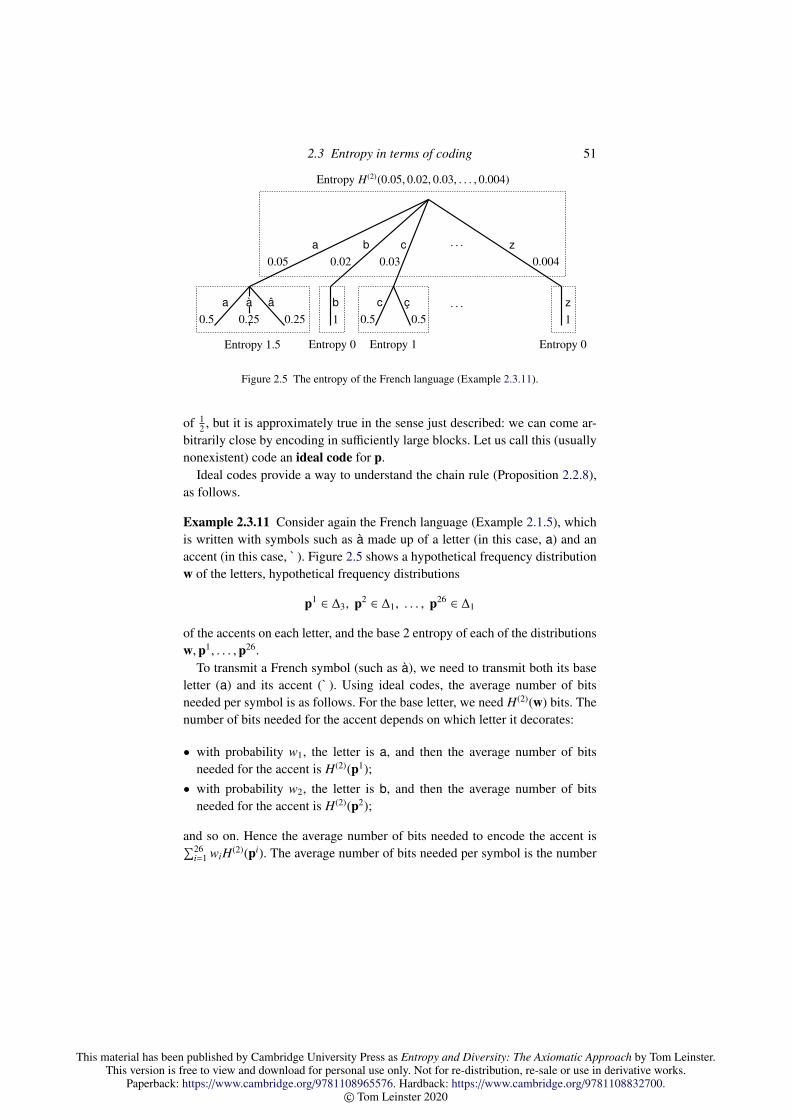
This material has been published by Cambridge University Press as Entropy and Diversity: The Axiomatic Approach by Tom Leinster.This version is free to view and download for personal use only. Not for re-distribution, re-sale or use in derivative works.
Paperback: https://www.cambridge.org/9781108965576. Hardback: https://www.cambridge.org/9781108832700.© Tom Leinster 2020
2.3 Entropy in terms of coding 51
0.05 0.02 0.03 0.004a b c · · · z
a a a b c c z0.5 0.25 0.25 1 0.5 0.5 1
· · ·
Entropy H(2)(0.05, 0.02, 0.03, . . . , 0.004)
Entropy 1.5 Entropy 0 Entropy 1 Entropy 0
Figure 2.5 The entropy of the French language (Example 2.3.11).
of 12 , but it is approximately true in the sense just described: we can come ar-
bitrarily close by encoding in sufficiently large blocks. Let us call this (usuallynonexistent) code an ideal code for p.
Ideal codes provide a way to understand the chain rule (Proposition 2.2.8),as follows.
Example 2.3.11 Consider again the French language (Example 2.1.5), whichis written with symbols such as a made up of a letter (in this case, a) and anaccent (in this case, ` ). Figure 2.5 shows a hypothetical frequency distributionw of the letters, hypothetical frequency distributions
p1 ∈ ∆3, p2 ∈ ∆1, . . . , p26 ∈ ∆1
of the accents on each letter, and the base 2 entropy of each of the distributionsw,p1, . . . ,p26.
To transmit a French symbol (such as a), we need to transmit both its baseletter (a) and its accent (` ). Using ideal codes, the average number of bitsneeded per symbol is as follows. For the base letter, we need H(2)(w) bits. Thenumber of bits needed for the accent depends on which letter it decorates:
• with probability w1, the letter is a, and then the average number of bitsneeded for the accent is H(2)(p1);
• with probability w2, the letter is b, and then the average number of bitsneeded for the accent is H(2)(p2);
and so on. Hence the average number of bits needed to encode the accent is∑26i=1 wiH(2)(pi). The average number of bits needed per symbol is the number

This material has been published by Cambridge University Press as Entropy and Diversity: The Axiomatic Approach by Tom Leinster.This version is free to view and download for personal use only. Not for re-distribution, re-sale or use in derivative works.
Paperback: https://www.cambridge.org/9781108965576. Hardback: https://www.cambridge.org/9781108832700.© Tom Leinster 2020
52 Shannon entropy
for the base letter plus the number for the accent, which is
H(2)(w) +
26∑i=1
wiH(2)(pi). (2.8)
On the other hand, we saw in Example 2.1.5 that the overall frequency distri-bution of the French symbols a, a, a, b, . . . , z is w (p1, . . . ,pn), whose idealcode uses
H(2)(w (p1, . . . ,pn))
(2.9)
bits per symbol. If we have reasoned correctly then the expressions (2.8)and (2.9) should be equal. The chain rule states that, indeed, they are.
2.4 Entropy in terms of diversity
Entropies of various kinds have been used to measure biological diversityfor almost as long as diversity measures have been considered. For instance,among all the measures of diversity used by ecologists, one of the most com-mon is the Shannon entropy H(p). Here p = (p1, . . . , pn) is the relative abun-dance distribution of the community concerned, as in Example 2.1.1. For rea-sons that will be explained, when it comes to measuring diversity, it is betterto use the exponential of entropy than entropy itself.
Let us begin by considering intuitively what it means for a community of nspecies to be diverse, for a fixed value of n. As described in the Introduction,there is a spectrum of viewpoints on what the word ‘diversity’ should mean.Loosely, though, diversity is low when most of the population is concentratedinto one or two very common species, and high when the population is spreadevenly across all species. Another way to say this is that diversity is low whenan individual chosen at random usually belongs to a common species, andhigh when an individual chosen at random usually belongs to a rare species.So, the diversity of a community can be understood as the average rarity of anindividual belonging to it.
Since pi represents the relative abundance of the ith species, 1/pi is a mea-sure of its rarity or specialness. We want to take the average rarity, and for nowwe will use the geometric mean as our notion of average. (Later, we will usedifferent notions of average. The most important are the power means, whichare introduced in Section 4.2 and include the geometric mean.) Thus, one rea-sonable measure of the diversity of a community is the geometric mean of the
This material has been published by Cambridge University Press as Entropy and Diversity: The Axiomatic Approach by Tom Leinster.This version is free to view and download for personal use only. Not for re-distribution, re-sale or use in derivative works.
Paperback: https://www.cambridge.org/9781108965576. Hardback: https://www.cambridge.org/9781108832700.© Tom Leinster 2020
2.4 Entropy in terms of diversity 53
species rarities 1/p1, . . . , 1/pn, weighted by the species sizes p1, . . . , pn:(1p1
)p1
· · ·
(1pn
)pn
.
We therefore make the following definition.
Definition 2.4.1 Let n ≥ 1 and p ∈ ∆n. The diversity of order 1 of p is
D(p) =1
pp11 pp2
2 · · · ppnn,
with the convention that 00 = 1.
Equivalently,
D(p) =∏
i∈supp(p)
p−pii = eH(p).
In short: diversity is the exponential of entropy.
Remarks 2.4.2 i. The meaning of ‘order 1’ will be revealed in Section 4.3.It is related to the different possible notions of average. In this section,‘diversity’ will always mean diversity of order 1.
ii. No choice of base is involved in the definition of D, in contrast to the sit-uation for H (Remark 2.2.1). For instance, D(p) is equal to both eH(p) and2H(2)(p).
Crucially, the word ‘diversity’ refers only to the relative, not absolute, abun-dances. If half of a forest burns down, or if a patient loses 90% of their gutbacteria, then it may be an ecological or medical disaster; but assuming thatthe system is well-mixed, the diversity does not change. In the language ofphysics, diversity is an intensive quantity (like density or temperature) ratherthan an extensive quantity (like mass or heat), meaning that it is independentof the system’s size.
Lemma 2.2.4 immediately implies:
Lemma 2.4.3 Let n ≥ 1.
i. D(p) ≥ 1 for all p ∈ ∆n, with equality if and only if pi = 1 for somei ∈ 1, . . . , n.
ii. D(p) ≤ n for all p ∈ ∆n, with equality if and only if p = un.
Similarly, the continuity of entropy (Lemma 2.2.5) immediately implies:
Lemma 2.4.4 For each n ≥ 1, the diversity function D : ∆n → R of order 1 iscontinuous.
This material has been published by Cambridge University Press as Entropy and Diversity: The Axiomatic Approach by Tom Leinster.This version is free to view and download for personal use only. Not for re-distribution, re-sale or use in derivative works.
Paperback: https://www.cambridge.org/9781108965576. Hardback: https://www.cambridge.org/9781108832700.© Tom Leinster 2020
54 Shannon entropy
Evidently
D(un) = n
for all n ≥ 1. This is a very important property for a diversity measure, and weadopt the standard terminology for it:
Definition 2.4.5 Let(E : ∆n → (0,∞)
)n≥1 be a sequence of functions. Then E
is an effective number if E(un) = n for all n ≥ 1.
Thus, D is an effective number. When the species are all present in equalquantities, we think of the community as containing n fully present speciesand assign it a diversity value of n. On the other hand, if one species accountsfor nearly 100% of the community and all the others are very rare, then the di-versity value is barely more than 1 (by Lemmas 2.4.3(i) and 2.4.4). Effectively,there is barely more than one species present.
For instance, if a community has a diversity of 18.2, then the community isslightly more diverse than a community of 18 equally abundant species. Thereare ‘effectively’ slightly more than 18 balanced species.
Examples 2.4.6 For the four distributions on 1, 2, 3, 4 in Examples 2.2.2, thediversities are
22 = 4, 27/4 ≈ 3.364, 21 = 2, 20 = 1,
respectively. In particular, the community represented by the second distribu-tion is judged by D to be somewhat more diverse than a community of threespecies in equal proportions, but less diverse than a balanced community offour species.
Despite the popularity of Shannon entropy as a measure of biological di-versity, many ecologists have argued that it should be rejected in favour ofits exponential, including MacArthur [235] in 1965, Buzas and Gibson [56]in 1969, and Whittaker [349] in 1972. More recently and more generally,Jost [164, 165, 167] has argued convincingly that when measuring diversity,we should only use effective numbers. (That principle appears to be gainingacceptance, judging by the editorial [89] of Ellison.) The following example isadapted from Jost [165].
Example 2.4.7 Suppose that a plague strikes a continent of a million equallycommon species, rendering 90% of the species extinct and leaving the remain-ing 10% untouched. How do H and D respond to this catastrophe?
The Shannon entropy H drops by just
1 −log(105)log(106)
=16≈ 17%,

This material has been published by Cambridge University Press as Entropy and Diversity: The Axiomatic Approach by Tom Leinster.This version is free to view and download for personal use only. Not for re-distribution, re-sale or use in derivative works.
Paperback: https://www.cambridge.org/9781108965576. Hardback: https://www.cambridge.org/9781108832700.© Tom Leinster 2020
2.4 Entropy in terms of diversity 55
suggesting a change of considerably smaller magnitude than the one that actu-ally occurred. For comparison, if a community of four equally common speciesloses only one of its species, the rest remaining unchanged, this causes a dropin Shannon entropy of
1 −log 3log 4
≈ 21%.
So, if we judge by percentage change in Shannon entropy, losing 25% of fourspecies destroys a greater proportion of the diversity than losing 90% of amillion species. Shannon entropy drops more in the situation where the speciesloss is less. So as an indicator of change in diversity, percentage change inShannon entropy is plainly unsuitable.
However, the effect of the plague on the diversity D is to make it drop by90% (from 106 to 105), because D is an effective number. And for the samereason, in the four-species example, D drops by 25% (from 4 to 3). This isintuitively reasonable behaviour, faithfully reflecting the scale of the change.
In information and coding theory, the logarithmic measure H is the moreuseful form, corresponding as it does to the number of bits per symbol in anideal code. But for species diversity, it is the number of species (not its loga-rithm) with which we reason most naturally.
We now consider the chain rule in terms of diversity. Taking exponentials inProposition 2.2.8 gives:
Corollary 2.4.8 Let n, k1, . . . , kn ≥ 1. Then
D(w (p1, . . . ,pn)
)= D(w) ·
n∏i=1
D(pi)wi
for all w ∈ ∆n and pi ∈ ∆ki .
The second factor on the right-hand side is the geometric mean of the diver-sities D(p1), . . . ,D(pn), weighted by w1, . . . ,wn.
The most important aspect of this result is not the specific formula, but thefact that the diversity of the composite distribution depends only on w andD(p1), . . . ,D(pn), not on p1, . . . ,pn themselves. This can be understood in ei-ther of the following ways.
Example 2.4.9 As in Example 2.1.6, consider a group of n islands of relativesizes w1, . . . ,wn, with no species shared between islands. Let di denote D(pi),the diversity of the ith island. Then the diversity of the whole island group is
D(w) · dw11 · · · d
wnn . (2.10)

This material has been published by Cambridge University Press as Entropy and Diversity: The Axiomatic Approach by Tom Leinster.This version is free to view and download for personal use only. Not for re-distribution, re-sale or use in derivative works.
Paperback: https://www.cambridge.org/9781108965576. Hardback: https://www.cambridge.org/9781108832700.© Tom Leinster 2020
56 Shannon entropy
Thus, the diversity of the whole island group is determined by the diversitiesand relative sizes of the islands. It can be computed without reference to thepopulation distributions on each island.
Example 2.4.10 As in Example 2.1.7, consider a community of n genera, withthe ith genus divided into ki species. Let w denote the genus distribution anddi the diversity of the species in the ith genus. Then the species diversity of thewhole community is again given by (2.10). For instance, if there are 2 equallyabundant genera, with the first genus consisting of 45 species of equal abun-dance and the second consisting of 5 species of equal abundance, then thediversity of the whole community is
D(u2 (u45,u5)
)= D(u2) · D(u45)1/2D(u5)1/2 = 2
√45√
5 = 30.
In other words, the whole community of 45+5 = 50 species, which has relativeabundance distribution (
190 , . . . ,
190︸ ︷︷ ︸
45
, 110 , . . . ,
110︸ ︷︷ ︸
5
).
has the same diversity as a community of 30 species of equal abundance.
Different chain rules will appear in Sections 4.3 and 6.2, where we considerdiversity of orders other than 1. But all share the crucial property that D(w (p1, . . . ,pn)) depends only on w and D(p1), . . . ,D(pn).
We refer to this property of D as modularity. The word is used here inthe sense of modular software design, buildings or furniture (as opposed tomodular arithmetic or modules over a ring, say). In this metaphor, the islandsof Example 2.4.9 or the genera of Example 2.4.10 are the ‘modules’: whenit comes to computing the diversity of the whole assemblage, they are blackboxes whose internal features we do not need to know.
The logarithmic property of H (Corollary 2.2.10) translates into a multi-plicative property of D:
D(w ⊗ p) = D(w) · D(p) (2.11)
(n, k ≥ 1, w ∈ ∆n, p ∈ ∆k). An important special case is the replicationprinciple:
D(un ⊗ p) = nD(p)
(n, k ≥ 1, p ∈ ∆k). In the language of Example 2.4.9, this principle states thatgiven n islands of equal size and the same species distributions, but with noactual shared species, the diversity of the whole island group is n times thediversity of any individual island.

This material has been published by Cambridge University Press as Entropy and Diversity: The Axiomatic Approach by Tom Leinster.This version is free to view and download for personal use only. Not for re-distribution, re-sale or use in derivative works.
Paperback: https://www.cambridge.org/9781108965576. Hardback: https://www.cambridge.org/9781108832700.© Tom Leinster 2020
2.4 Entropy in terms of diversity 57
Another argument of Jost (adapted from [167] and [169]) makes a com-pelling case for the importance of the replication principle:
Example 2.4.11 An oil company is planning to carry out work on a group ofislands that will destroy all wildlife on half of the islands. Environmentalistsare bringing a legal case to stop them. What would be the impact of the workon biodiversity?
Suppose that there are 16 equally-sized islands in the group, that there areno species shared between islands, and that each island has diversity 4. Thenbefore the oil work, the diversity of the island group is
16 × 4 = 64.
Afterwards, similarly, it will be 32. Thus, the diversity is reduced by 50%.This is intuitively reasonable, and is a consequence of the replication principlefor D.
However, one of the most popular measures of diversity in ecology is Shan-non entropy (‘many long-term investigations have chosen it as their benchmarkof biological diversity’: Magurran [238], p. 101). The oil company’s lawyerscan therefore argue as follows. Before the works, the ‘diversity’ (Shannon en-tropy) is log 64, and afterwards, it will be log 32. Thus, the proportion of diver-sity preserved is
log 32log 64
=56≈ 83%.
On the other hand, the environmentalists’ lawyers can argue that the islandswhose wildlife is to be exterminated have a diversity of log 32, out of a total oflog 64, so the proportion of diversity destroyed will be
log 32log 64
=56≈ 83%.
So the oil company can truthfully claim that by the scientifically accepted mea-sure, 83% of the diversity will be preserved, while the environmentalists canjust as legitimately claim that 83% of the diversity will be lost. They cannotboth be right, and, of course, both are wrong: by any reasonable measure, 50%of the diversity is preserved and 50% is lost. The reason for the contradictoryand illogical conclusions is that Shannon entropy does not satisfy the replica-tion principle.
Although this is an idealized hypothetical example, it is not hard to see howa choice of diversity measure, far from being some obscure theoretical issue,could have genuine environmental consequences.
Although the diversity measure D does satisfy the replication principle, and

This material has been published by Cambridge University Press as Entropy and Diversity: The Axiomatic Approach by Tom Leinster.This version is free to view and download for personal use only. Not for re-distribution, re-sale or use in derivative works.
Paperback: https://www.cambridge.org/9781108965576. Hardback: https://www.cambridge.org/9781108832700.© Tom Leinster 2020
58 Shannon entropy
in that sense behaves logically, it has a glaring deficiency: it takes no noticeof the varying similarities between species. A forest consisting of ten equallyabundant species of larch is intuitively less diverse than a forest of ten equallyabundant but highly varied tree species. However, the measure D gives thesame diversity to both. The same criticism can be levelled at most of the diver-sity measures used in ecology, and a remedy is presented in Chapter 6.
2.5 The chain rule characterizes entropy
There are many characterizations of Shannon entropy, beginning with one inthe original paper by Shannon himself ([306], Theorem 2). Here, we prove avariant of one of the best-known such theorems, due to Dmitry Faddeev [94].
Theorem 2.5.1 (Faddeev) Let (I : ∆n → R)n≥1 be a sequence of functions.The following are equivalent:
i. the functions I are continuous and satisfy the chain rule
I(w (p1, . . . ,pn)
)= I(w) +
n∑i=1
wiI(pi)
(n, k1, . . . , kn ≥ 1, w ∈ ∆n, pi ∈ ∆ki );ii. I = cH for some c ∈ R.
In other words, up to a constant factor, entropy is uniquely characterizedby the chain rule and continuity. We already know that (ii) implies (i); thechallenge is to show that (i) implies (ii).
Remarks 2.5.2 i. As noted in Remark 2.2.1, the appearance of the constantfactor should not be a surprise. We could eliminate it by adding the axiomthat I(u2) = log 2, for instance.
ii. The theorem that Faddeev proved in [94] was slightly different. He assumedthat I was symmetric, that is, unchanged when the arguments p1, . . . , pn arepermuted, but he assumed only the superficially simpler form of the chainrule stated as equation (2.7) (Remark 2.2.11). As noted in that remark, ifwe assume symmetry then the two forms of the chain rule are equivalentvia a straightforward induction (Appendix A.1). On the other hand, Theo-rem 2.5.1 tells us that if we assume the chain rule in its general form thenwe do not need symmetry. This is not an obvious consequence of Faddeev’soriginal theorem.

This material has been published by Cambridge University Press as Entropy and Diversity: The Axiomatic Approach by Tom Leinster.This version is free to view and download for personal use only. Not for re-distribution, re-sale or use in derivative works.
Paperback: https://www.cambridge.org/9781108965576. Hardback: https://www.cambridge.org/9781108832700.© Tom Leinster 2020
2.5 The chain rule characterizes entropy 59
iii. If we assume symmetry, the hypotheses of Faddeev’s original theorem canbe weakened in a different direction, replacing continuity by measurability.This is a 1964 theorem of Lee [204]. We return to Lee’s theorem at the endof Chapter 11, but omit the proof.
iv. It is not possible to prove a Faddeev-type theorem with no regularity con-ditions at all (unless one drops the axiom of choice). Indeed, let f : R → Rbe an additive nonlinear function, as in Remark 1.1.9. Then the assignment
p 7→ −∑
i∈supp(p)
pi f (log pi)
satisfies the chain rule but is not a scalar multiple of Shannon entropy.
The remainder of this section is devoted to the proof of Theorem 2.5.1. Forthe rest of this section, let (I : ∆n → R)n≥1 be a sequence of continuous func-tions satisfying the chain rule.
The strategy of the proof is to show that I is proportional to H on suc-cessively larger classes of probability distributions. First we prove it for theuniform distributions un, using the results on logarithmic sequences in Sec-tion 1.2. This forms the bulk of the proof. It is then relatively easy to extendthe result to distributions p for which each pi is a positive rational number, andfrom there, by continuity, to all distributions.
We begin by studying the real sequence (I(un))n≥1.
Lemma 2.5.3 i. I(umn) = I(um) + I(un) for all m, n ≥ 1.
ii. I(u1) = 0.
Proof By the chain rule, I has the logarithmic property
I(w ⊗ p) = I(w (p, . . . ,p)
)= I(w) + I(p)
(w ∈ ∆m, p ∈ ∆n). In particular, for all m, n ≥ 1,
I(umn) = I(um ⊗ un) = I(um) + I(un),
proving (i). For (ii), take m = n = 1 in (i).
As we saw in Section 1.2, the property I(umn) = I(um)+ I(un) alone does nottell us very much about the sequence (I(un)). To take advantage of the resultsin that section, we will need to prove some analytic condition on the sequence.Specifically, we will show that I(un+1) − I(un) → 0 as n → ∞, then applyCorollary 1.2.3.
This material has been published by Cambridge University Press as Entropy and Diversity: The Axiomatic Approach by Tom Leinster.This version is free to view and download for personal use only. Not for re-distribution, re-sale or use in derivative works.
Paperback: https://www.cambridge.org/9781108965576. Hardback: https://www.cambridge.org/9781108832700.© Tom Leinster 2020
60 Shannon entropy
Lemma 2.5.4 I(1, 0) = 0.
Proof We compute I(1, 0, 0) in two ways. On the one hand, using the chainrule,
I(1, 0, 0) = I((1, 0)
((1, 0),u1
))= I(1, 0) + 1 · I(1, 0) + 0 · I(u1) = 2I(1, 0).
On the other, using the chain rule again and the fact that I(u1) = 0,
I(1, 0, 0) = I((1, 0)
(u1, (1, 0)
))= I(1, 0) + 1 · I(u1) + 0 · I(1, 0) = I(1, 0).
Hence I(1, 0) = 0.
Lemma 2.5.5 I(un+1) − nn+1 I(un)→ 0 as n→ ∞.
Proof We have
un+1 =
( nn + 1
,1
n + 1
) (un,u1),
so by the chain rule and the fact that I(u1) = 0,
I(un+1) = I( nn + 1
,1
n + 1
)+
nn + 1
I(un).
Hence
I(un+1) −n
n + 1I(un) = I
( nn + 1
,1
n + 1
)→ I(1, 0) = 0
as n→ ∞, by continuity and Lemma 2.5.4.
Now we can use the results of Section 1.2.
Lemma 2.5.6 There exists a constant c ∈ R such that I(un) = cH(un) for alln ≥ 1.
Proof By Lemma 2.5.3(i), the sequence (I(un)) is logarithmic. By Lem-mas 2.5.5 and 1.2.4, limn→∞
(I(un+1) − I(un)
)= 0. Hence by Corollary 1.2.3,
there is some c ∈ R such that for all n ≥ 1,
I(un) = c log n = cH(un).
We now move to the second phase of the proof of Theorem 2.5.1. Let c bethe constant of Lemma 2.5.6 (which is uniquely determined).
Lemma 2.5.7 Let p ∈ ∆n with p1, . . . , pn rational and nonzero. Then I(p) =
cH(p).
This material has been published by Cambridge University Press as Entropy and Diversity: The Axiomatic Approach by Tom Leinster.This version is free to view and download for personal use only. Not for re-distribution, re-sale or use in derivative works.
Paperback: https://www.cambridge.org/9781108965576. Hardback: https://www.cambridge.org/9781108832700.© Tom Leinster 2020
2.5 The chain rule characterizes entropy 61
Proof We can write
p =
(k1
k, . . . ,
kn
k
)for some positive integers k1, . . . , kn, where k = k1 + · · · + kn. Then
p (uk1 , . . . ,ukn ) = uk.
Since I satisfies the chain rule and I(ur) = cH(ur) for all r ≥ 1, we have
I(p) +
n∑i=1
pi · cH(uki ) = cH(uk).
But since cH satisfies the chain rule too, we also have
cH(p) +
n∑i=1
pi · cH(uki ) = cH(uk).
The result follows.
The third and final phase of the proof is trivial: since the probability dis-tributions with positive rational probabilities are dense in the space ∆n of allprobability distributions, and since I and cH are continuous functions agreeingon this dense set, they are equal everywhere. This proves Theorem 2.5.1.
Like any result on entropy, Faddeev’s theorem can be translated into diver-sity terms. In the following corollary, we eliminate the arbitrary constant factorby requiring that E be an effective number.
Corollary 2.5.8 Let(E : ∆n → (0,∞)
)n≥1 be a sequence of functions. The fol-
lowing are equivalent:
i. the functions E are continuous and satisfy the chain rule
E(w (p1, . . . ,pn)
)= E(w) ·
n∏i=1
E(pi)wi (2.12)
(n, k1, . . . , kn ≥ 1, w ∈ ∆n, pi ∈ ∆ki ), and E is an effective number;ii. E = D.
Proof By Faddeev’s theorem applied to log E, the sequences of continuousfunctions E satisfying the diversity chain rule (2.12) are exactly the real powersDc (c ∈ R). But the effective number property (or indeed, the single equationE(u2) = 2) then forces c = 1.

This material has been published by Cambridge University Press as Entropy and Diversity: The Axiomatic Approach by Tom Leinster.This version is free to view and download for personal use only. Not for re-distribution, re-sale or use in derivative works.
Paperback: https://www.cambridge.org/9781108965576. Hardback: https://www.cambridge.org/9781108832700.© Tom Leinster 2020
3
Relative entropy
The notion of relative entropy allows us to compare two probability distribu-tions on the same space. More specifically, for each pair of probability distri-butions p, r on the same finite set, there is defined a real number H(p ‖ r) ≥ 0,the entropy of p relative to r. It is zero just when p = r. It extends the def-inition of Shannon entropy, in the sense that the Shannon entropy of a singledistribution p on 1, . . . , n is a function of H(p ‖ un), the entropy of p relativeto the uniform distribution.
Relative entropy goes by a remarkable number of names, attesting toits wide variety of interpretations and uses. It is also known as Kullback–Leibler information (as in [302], for instance), Kullback–Leibler distance [69],Kullback–Leibler divergence [171], directed divergence [196], information di-vergence [127], information deficiency [46], amount of information [291], dis-crimination information [197], relative information [321], gain of informationor information gain ([292], Section IX.4), discrimination distance [178], anderror [184], among others. This chapter provides multiple explanations andapplications of relative entropy, as well as a theorem pinpointing what makesrelative entropy uniquely useful.
Our first explanation of relative entropy is in terms of coding (Section 3.2).As we saw in Section 2.3, the Shannon entropy of p gives the average numberof bits per symbol needed to encode an alphabet with frequency distributionp in a coding system optimized for that purpose. In a similar sense, H(p ‖ r)measures the extra number of bits per symbol needed to encode an alphabetwith frequencies p using a coding system that was optimized for the frequencydistribution r. In other words, it is the penalty for using the wrong system.
The exponential of relative entropy is called relative diversity (Section 3.3).Often we have a preconceived idea of what an ordinary or default distributionof species is, and we judge how unusual a community is relative to that expec-tation. For instance, if we were assessing the diversity of flowering plants in a
62
This material has been published by Cambridge University Press as Entropy and Diversity: The Axiomatic Approach by Tom Leinster.This version is free to view and download for personal use only. Not for re-distribution, re-sale or use in derivative works.
Paperback: https://www.cambridge.org/9781108965576. Hardback: https://www.cambridge.org/9781108832700.© Tom Leinster 2020
3.1 Definition and properties of relative entropy 63
particular region of the island of Tasmania, we would naturally judge it by thestandards of Tasmania as a whole. The relative diversity exp(H(p ‖ r)) reflectsthe unusualness of a community with distribution p relative to a reference dis-tribution r.
Section 3.4 gives short accounts of roles played by relative entropy in threeother subjects. In measure theory, we find that the definition of relative en-tropy generalizes easily from finite sets to arbitrary measurable spaces, whileordinary Shannon entropy does not. The slogan is: all entropy is relative. Ingeometry, although H(− ‖ −) does not define a distance function on the set ∆n
of distributions, it turns out that infinitesimally, it behaves like the square of adistance. We can extend this infinitesimal metric to a global metric in the man-ner of Riemannian geometry. In statistics, the second argument r of H(p ‖ r)should be thought of as a prior, and maximizing likelihood can be reinterpretedas minimizing relative entropy. The concept of relative entropy also gives riseto the notions of Fisher information and the Jeffreys prior, an objective priordistribution in the sense of Bayesian statistics.
We finish the chapter with a characterization theorem for relative entropy(Section 3.5), which first appeared in [216]. Just as for Faddeev’s character-ization of ordinary entropy, the main characterizing property is a chain rule.And just as for ordinary entropy, many characterization theorems for relativeentropy have previously been proved; but the one presented here appears to bethe simplest yet.
3.1 Definition and properties of relative entropy
This short section presents the definition and basic properties of relative en-tropy, without motivation for now. The later sections provide multiple inter-pretations of, and justifications for, the definition.
Definition 3.1.1 Let n ≥ 1 and p, r ∈ ∆n. The entropy of p relative to r is
H(p ‖ r) =∑
i∈supp(p)
pi logpi
ri. (3.1)
If there is some i such that pi > 0 = ri then H(p ‖ r) is defined to be∞.
In the literature, relative entropy is more often denoted by D(p ‖ r), but inthis text, we reserve the letter D for measures of diversity.

This material has been published by Cambridge University Press as Entropy and Diversity: The Axiomatic Approach by Tom Leinster.This version is free to view and download for personal use only. Not for re-distribution, re-sale or use in derivative works.
Paperback: https://www.cambridge.org/9781108965576. Hardback: https://www.cambridge.org/9781108832700.© Tom Leinster 2020
64 Relative entropy
Example 3.1.2 Let p ∈ ∆n. Then
H(p ‖ un) =∑
i∈supp(p)
pi log(npi)
= log n − H(p)
= H(un) − H(p).
Thus, ordinary entropy is essentially a special case of relative entropy.
Example 3.1.3 As well as sometimes taking the value∞, relative entropy cantake arbitrarily large finite values (even for fixed n). For instance, for t ∈ (0, 1),
H(u2 ‖ (t, 1 − t)
)=
12
log12t
+12
log1
2(1 − t)→ ∞
as t → 0.
Unless p = r, there are some values of i for which pi > ri and others forwhich pi < ri. Hence, some of the summands in (3.1) are positive and othersare negative. Nevertheless:
Lemma 3.1.4 H(p ‖ r) ≥ 0, with equality if and only if p = r.
Proof If pi > 0 = ri for some i then H(p ‖ r) = ∞. Suppose otherwise, so thatsupp(p) ⊆ supp(r). Using Lemma 2.2.3,
H(p ‖ r) = −∑
i∈supp(p)
pi logri
pi
≥ − log( ∑
i∈supp(p)
piri
pi
)
≥ − log( ∑
i∈supp(r)
ri
)= − log 1 = 0,
with equality in the first inequality if and only if ri/pi = r j/p j for alli, j ∈ supp(p). Equality holds in the second inequality if and only if supp(p) =
supp(r). Hence for equality to hold throughout, there must be some constant αsuch that ri = αpi for all i ∈ supp(p) = supp(r). But since
∑i∈supp(p) pi = 1 =∑
i∈supp(r) ri, this forces α = 1 and so p = r.
Lemma 3.1.4 suggests that very roughly speaking, H(p ‖ r) can be under-stood as a kind of distance between p and r. However, relative entropy doesnot satisfy the triangle inequality (Example 3.4.2). Nor is it symmetric: foras Examples 3.1.2 and 3.1.3 show, H(p ‖ u2) ≤ log 2 for all p ∈ ∆2, whereas

This material has been published by Cambridge University Press as Entropy and Diversity: The Axiomatic Approach by Tom Leinster.This version is free to view and download for personal use only. Not for re-distribution, re-sale or use in derivative works.
Paperback: https://www.cambridge.org/9781108965576. Hardback: https://www.cambridge.org/9781108832700.© Tom Leinster 2020
3.1 Definition and properties of relative entropy 65
H(u2 ‖p) can be arbitrarily large. We will return to the interpretation of relativeentropy as a measure of distance in Section 3.4.
We now list some of the basic properties of relative entropy. Matters aresimplified if we restrict to just those pairs (p, r) such that H(p ‖ r) < ∞. Forn ≥ 1, write
An = (p, r) ∈ ∆n × ∆n : ri = 0 =⇒ pi = 0
= (p, r) ∈ ∆n × ∆n : supp(p) ⊆ supp(r).
Then
H(p ‖ r) < ∞ ⇐⇒ (p, r) ∈ An.
So for each n ≥ 1, we have the function
H(− ‖ −) : An → R
(p, r) 7→ H(p ‖ r).
This sequence of functions has the following properties, among others.
Measurability in the second argument. For each fixed p ∈ ∆n, the function
r ∈ ∆n : (p, r) ∈ An → R
r 7→ H(p ‖ r)
is measurable. Indeed, the function H(− ‖ −) : An → R is continu-ous, but for the unique characterization of relative entropy proved inSection 3.5, measurability in the second argument is all we will need.
Permutation-invariance. The relative entropy H(p ‖ r) is unchanged if thesame permutation is applied to the indices of both p and r. That is,
H(p ‖ r) = H(pσ ‖ rσ)
for all (p, r) ∈ An and permutations σ of 1, . . . , n, where
pσ = (pσ(1), . . . , pσ(n)) (3.2)
and similarly rσ.Vanishing. H(p ‖ p) = 0 for all p ∈ ∆n.Chain rule. Let n, k1, . . . , kn ≥ 1 and
(w, w) ∈ An,(p1, p1) ∈ Ak1 , . . . ,
(pn, pn) ∈ Akn .
Then
H(w (p1, . . . ,pn) ‖ w (p1, . . . , pn)
)= H(w ‖ w) +
n∑i=1
wiH(pi ‖ pi).
(3.3)

This material has been published by Cambridge University Press as Entropy and Diversity: The Axiomatic Approach by Tom Leinster.This version is free to view and download for personal use only. Not for re-distribution, re-sale or use in derivative works.
Paperback: https://www.cambridge.org/9781108965576. Hardback: https://www.cambridge.org/9781108832700.© Tom Leinster 2020
66 Relative entropy
This is a straightforward check, similar to Proposition 2.2.8. Note that(w (p1, . . . ,pn), w (p1, . . . , pn)
)∈ Ak1+···+kn ,
so the relative entropy of this pair is guaranteed to be finite.As a special case, relative entropy has a logarithmic property:
H(w ⊗ p ‖ w ⊗ p) = H(w ‖ w) + H(p ‖ p) (3.4)
for all (w, w) ∈ An and (p, p) ∈ Ak. This follows from the chain ruleby taking ki = k, pi = p and pi = p for all i ∈ 1, . . . , n.
Just as for ordinary entropy, different choices of the base of the logarithm inthe definition of relative entropy only change it by a constant factor. We willsee in Section 3.5 that up to a constant factor, the four properties just listedcharacterize relative entropy uniquely.
3.2 Relative entropy in terms of coding
We have already interpreted Shannon entropy in terms of coding (Section 2.3).Here we do the same for relative entropy.
To help our understanding, let us regard a probability distribution p ∈ ∆n
as the frequency distribution of the n symbols in some human language, whichwe call language p. We make use of the convenient fiction introduced on p. 50,imagining that there exists an ideal code for language p: a code whose averageword length is exactly H(2)(p). We will suppose that the encoding is performedby a machine, called machine p. Although most distributions p have no idealcode, one can come arbitrarily close (as in Section 2.3), and this justifies theuse of ideal codes as an explanatory device.
For p ∈ ∆n, the ordinary base 2 entropy
H(2)(p) =∑
i∈supp(p)
pi log21pi
satisfies
H(2)(p) = no. bits/symbol to encode language p using machine p.
Now let p, r ∈ ∆n, with p and r viewed as the frequency distributions of twolanguages on the same set of symbols. Write
H(2)(p ‖ r) =∑
i∈supp(p)
pi log2pi
ri=
H(p ‖ r)log 2
This material has been published by Cambridge University Press as Entropy and Diversity: The Axiomatic Approach by Tom Leinster.This version is free to view and download for personal use only. Not for re-distribution, re-sale or use in derivative works.
Paperback: https://www.cambridge.org/9781108965576. Hardback: https://www.cambridge.org/9781108832700.© Tom Leinster 2020
3.2 Relative entropy in terms of coding 67
for the base 2 relative entropy. We will interpret H(2)(p‖r) in terms of languagesp and r and machines p and r.
To do this, first consider the quantity
H(2)×(p ‖ r) =∑
i∈supp(p)
pi log21ri.
Here log2(1/ri) is the number of bits that machine r uses to encode the ithsymbol. (Of course, this is not usually an integer, but recall the comments onideal codes on p. 51.) Hence
H(2)×(p ‖ r) = no. bits/symbol to encode language p using machine r.
This quantity H(2)×(p ‖ r), or its base e analogue
H×(p ‖ r) =∑
i∈supp(p)
pi log1ri
= H(2)×(p ‖ r) · log 2, (3.5)
is the cross entropy of p with respect to r.The relative, cross and ordinary entropies are related by the equation
H(p ‖ r) = H×(p ‖ r) − H(p). (3.6)
Hence
H(2)(p ‖ r) = H(2)×(p ‖ r) − H(2)(p)
= no. bits/symbol to encode language p using machine r− no. bits/symbol to encode language p using machine p.
So, for the task of encoding language p, the relative entropy H(2)(p ‖ r) isthe number of extra bits needed if one uses machine r instead of machine p.Machine p is ideal for the job: it is optimized for exactly this purpose. Relativeentropy is, then, the penalty for using the wrong machine.
This provides an intuitive explanation of why H(p‖r) is always nonnegativeand why H(p ‖ p) = 0. It also suggests why relative entropy can be arbitrarilylarge, as in the following example.
Examples 3.2.1 i. Consider an alphabet with n = 2 symbols. Suppose thatlanguage p uses the two symbols with equal frequency, and that in languager the frequency distribution is (2−1000, 1 − 2−1000). Then machine r encodesthe first symbol with a word of 1000 bits. Since language p uses this symbolhalf the time, the average word length when encoding language p usingmachine r is at least 500 bits. This is drastically worse than when languagep is encoded using the most suitable machine, machine p, which has an

This material has been published by Cambridge University Press as Entropy and Diversity: The Axiomatic Approach by Tom Leinster.This version is free to view and download for personal use only. Not for re-distribution, re-sale or use in derivative works.
Paperback: https://www.cambridge.org/9781108965576. Hardback: https://www.cambridge.org/9781108832700.© Tom Leinster 2020
68 Relative entropy
average word length of just 1 bit. So the relative entropy H(2)(p ‖ r) is atleast 499.
ii. The same example provides intuition for the fact that
H(p ‖ r) , H(r ‖ p).
Machine p encodes the two symbols of the alphabet as the binary words0 and 1, of length 1 each. Hence the average number of bits used whenencoding language r (or indeed, any other language) in machine p is 1. SoH(2)(r ‖ p) is less than 1, and is therefore much smaller than the value ofH(2)(p ‖ r) derived in (i).
Remark 3.2.2 The name ‘cross entropy’ has a tangled history. It was intro-duced by Jack Good in 1955 ([119], Section 6), who defined it as in equa-tion (3.5) above and gave it its name. But later, Good used ‘cross entropy’ asa synonym for relative entropy ([120], p. 913), and others have done the same(Shore and Johnson [310], for instance). Nowadays the term is often used inthe context of the cross entropy method in operational research [77]. In thebroadest terms, this involves fixing a distribution p and minimizing H(p‖r), orequivalently H×(p ‖ r), among all r subject to certain constraints. It makes nodifference which one minimizes, by equation (3.6). From that point of view,the concepts are essentially interchangeable, which has not helped to clarifythe terminological situation either.
This text uses the term with its original meaning, in part because relativeentropy already has an overabundance of synonyms.
The chain rule for relative entropy (equation (3.3)) can also be explained interms of coding, as in the following example.
Example 3.2.3 In Example 2.3.11, we interpreted the chain rule for ordinaryShannon entropy in terms of letters and their accents in French. There are manydialects of French, using the same letters and accents but slightly differentvocabulary, hence slightly different frequency distributions of both letters andaccents. Here we consider Swiss and Canadian French, which for brevity wecall just ‘Swiss’ and ‘Canadian’.
Define distributions w, w,pi, pi as follows:
w ∈ ∆26 : frequency distribution of letters in Swiss
w ∈ ∆26 : frequency distribution of letters in Canadian

This material has been published by Cambridge University Press as Entropy and Diversity: The Axiomatic Approach by Tom Leinster.This version is free to view and download for personal use only. Not for re-distribution, re-sale or use in derivative works.
Paperback: https://www.cambridge.org/9781108965576. Hardback: https://www.cambridge.org/9781108832700.© Tom Leinster 2020
3.2 Relative entropy in terms of coding 69
and then
p1 ∈ ∆3 : frequency distribution of accents on a in Swiss
p1 ∈ ∆3 : frequency distribution of accents on a in Canadian...
p26 ∈ ∆1 : frequency distribution of accents on z in Swiss
p26 ∈ ∆1 : frequency distribution of accents on z in Canadian.
So, recalling the convention that a ‘symbol’ is a letter plus a (possibly nonex-istent) accent,
w (p1, . . . ,p26) = frequency distribution of symbols in Swiss
w (p1, . . . , p26) = frequency distribution of symbols in Canadian.
Now suppose that we encode Swiss using the Canadian machine. How muchextra does this cost (in bits/symbol) compared to encoding Swiss using theSwiss machine?
Since every symbol consists of a letter with an accent, we expect to have:
mean extra cost per symbol =
mean extra cost per letter + mean extra cost per accent. (3.7)
The mean extra cost per symbol is
H(2)(w (p1, . . . ,p26) ‖ w
(p1, . . . , p26)).
The mean extra cost per letter is
H(2)(w ‖ w).
The mean extra cost per accent is computed by conditioning on the letter thatit decorates. Since it is Swiss rather than Canadian that we are encoding, theprobability of the ith letter occurring is wi, so the mean extra cost per accent is
26∑i=1
wiH(2)(pi ‖ pi).Hence the hoped-for equation (3.7) predicts that
H(2)(w (p1, . . . ,p26) ‖ w
(p1, . . . , p26)) = H(2)(w ‖ w) +
26∑i=1
wiH(2)(pi ‖ pi).This is indeed true. It is exactly the chain rule of Section 3.1.
This material has been published by Cambridge University Press as Entropy and Diversity: The Axiomatic Approach by Tom Leinster.This version is free to view and download for personal use only. Not for re-distribution, re-sale or use in derivative works.
Paperback: https://www.cambridge.org/9781108965576. Hardback: https://www.cambridge.org/9781108832700.© Tom Leinster 2020
70 Relative entropy
3.3 Relative entropy in terms of diversity
In Section 2.4, we interpreted the exponential of Shannon entropy as the di-versity of a biological community. Here we interpret the exponential of rela-tive entropy as a measure of how diverse or atypical one community is whenseen from the perspective of another. This interpretation elaborates on ideas ofReeve et al. [290].
As in Section 2.4, we consider communities of individuals drawn from nspecies, whose relative abundances define a probability distribution on the set1, . . . , n.
Definition 3.3.1 Let n ≥ 1 and p, r ∈ ∆n. The diversity of p relative to r (oforder 1) is
D(p ‖ r) = eH(p‖r) =∏
i∈supp(p)
( pi
ri
)pi
∈ [1,∞].
(We repeat the warning that although in the literature, the notation D(p ‖ r)is often used to mean relative entropy, we reserve the letter D for diversity.)
By Lemma 3.1.4, D(p ‖ r) ≥ 1, with equality if and only if p = r.It is helpful to regard r as the distribution of a reference community (a com-
munity that one considers to be normal or the default) and p as the distributionof the community in which we are primarily interested. As we will see, D(p‖r)measures how exotic or unusual this other community is from the viewpoint ofthe reference community.
To explain this, it is helpful to begin with another quantity:
Definition 3.3.2 Let n ≥ 1 and p, r ∈ ∆n. The cross diversity of p with re-spect to r (of order 1) is
D×(p ‖ r) = eH×(p‖r) =∏
i∈supp(p)
( 1ri
)pi
∈ [1,∞].
In Section 2.4, the ordinary diversity of p,
D(p) =∏
i∈supp(p)
( 1pi
)pi
,
was interpreted as follows: 1/pi is the rarity of the ith species within the com-munity, and D(p) is therefore the average rarity of individuals in the commu-nity. (In this case, ‘average’ means geometric mean.) Cross diversity can beunderstood in a similar way. If we use the second community r as our ref-erence point – the community by which others are to be judged – then wenaturally take the rarity or specialness of the ith species to be 1/ri rather than

This material has been published by Cambridge University Press as Entropy and Diversity: The Axiomatic Approach by Tom Leinster.This version is free to view and download for personal use only. Not for re-distribution, re-sale or use in derivative works.
Paperback: https://www.cambridge.org/9781108965576. Hardback: https://www.cambridge.org/9781108832700.© Tom Leinster 2020
3.3 Relative entropy in terms of diversity 71
1/pi. Thus, D×(p ‖r) is the average rarity of individuals in the first community,seen from the viewpoint of the second.
Since
D(p ‖ r) =D×(p ‖ r)
D(p), (3.8)
the relative diversity measures how much more diverse the first communitylooks from the viewpoint of the second than from the viewpoint of itself. Someexamples illuminate this interpretation.
Example 3.3.3 We have D(p ‖ p) = 1, which is the minimal possible value ofrelative diversity: any community perceives itself as completely normal.
Example 3.3.4 Let p and r be the relative abundance distributions of reptilesin Portugal and Russia, respectively. Geckos are commonplace in Portugal butrare in Russia. Hence from the Russian viewpoint, the ecology of Portugalseems exotic or atypical, in this respect at least.
Mathematically, there are several values of i (corresponding to species ofgecko) such that ri is small but pi is not. This means that the cross diversitycontains some large factors, (1/ri)pi , and the relative diversity also containssome large factors, (pi/ri)pi . Thus, both the cross diversity D×(p ‖ r) and therelative diversity D(p ‖ r) are large, regardless of the diversity D(p) of reptilesin Portugal.
Example 3.3.5 Taking the previous example to the extreme, if one or morespecies is present in the test community p but absent in the reference commu-nity r then D(p ‖ r) = ∞.
Example 3.3.6 Suppose now that we judge communities from the referencepoint of a community with a uniform distribution. (This is in some sense thecanonical choice of reference, and is the one produced by the maximum en-tropy method of statistics [154, 51].) The cross diversity D×(p ‖ un) is equal ton, regardless of p. Hence equation (3.8) gives
D(p ‖ un) =n
D(p). (3.9)
This is also the exponential of the equation
H(p ‖ un) = log n − H(p)
derived in Example 3.1.2.Equation (3.9) implies that for a fixed number of species, the diversity of a
community relative to the uniform distribution is inversely proportional to theintrinsic diversity of the community itself. From the viewpoint of a community

This material has been published by Cambridge University Press as Entropy and Diversity: The Axiomatic Approach by Tom Leinster.This version is free to view and download for personal use only. Not for re-distribution, re-sale or use in derivative works.
Paperback: https://www.cambridge.org/9781108965576. Hardback: https://www.cambridge.org/9781108832700.© Tom Leinster 2020
72 Relative entropy
in which all n species are balanced equally, any variation from this balancelooks unusual – and the more unbalanced, the more unusual.
As an illustration of the general point, house sparrows are common through-out Britain, but a region of the country in which the only birds were house spar-rows would be highly unusual. Correspondingly, the relative diversity D(p ‖ r)of that region relative to the country would be high, even though the intrinsicdiversity D(p) of the region would take the minimum possible value, 1.
By equation (3.9) and Lemma 2.4.3, D(p ‖ un) takes its minimal value, 1,when p = un. It takes its maximal value, n, when
p = (0, . . . , 0, 1, 0, . . . , 0).
That is, from the viewpoint of a completely balanced community, the mostunusual possible community is one consisting of a single species.
Often, we want to assess a community from the viewpoint of a larger com-munity that contains it. For instance, we are more likely to study the diversityof plankton in the eastern Mediterranean Sea with reference to the Mediter-ranean as a whole than with reference to the Arctic Ocean.
Consider, then, an ecological community with relative abundance distribu-tion r ∈ ∆n, and a subcommunity consisting of some of its organisms. Writeπi for the proportion of the community consisting of individuals that belong toboth the subcommunity and the ith species. Then 0 ≤ πi ≤ ri. The proportionof the whole community made up by the subcommunity is w =
∑πi ≤ 1, and
the relative abundance distribution of the subcommunity is
p = (π1/w, . . . , πn/w) ∈ ∆n.
The inequality πi ≤ ri gives wpi ≤ ri, or equivalently,
pi
ri≤
1w, (3.10)
for all i ∈ supp(r). Hence
D(p ‖ r) =∏
i∈supp(p)
( pi
ri
)pi
≤∏
i∈supp(p)
( 1w
)pi
=1w,
giving
1 ≤ D(p ‖ r) ≤1w. (3.11)
We now consider cases in which these bounds are attained.
Examples 3.3.7 i. By Lemma 3.1.4, D(p ‖ r) attains its lower bound of 1precisely when p = r. This means that the subcommunity is exactly typicalor representative of the larger community; it is minimally unusual.

This material has been published by Cambridge University Press as Entropy and Diversity: The Axiomatic Approach by Tom Leinster.This version is free to view and download for personal use only. Not for re-distribution, re-sale or use in derivative works.
Paperback: https://www.cambridge.org/9781108965576. Hardback: https://www.cambridge.org/9781108832700.© Tom Leinster 2020
3.3 Relative entropy in terms of diversity 73
pq
r
Figure 3.1 The three communities of Example 3.3.8.
ii. The maximum D(p ‖ r) = 1/w in (3.11) is attained when ri = wpi forall i ∈ supp(p). In the notation above, this is equivalent to πi = ri for alli ∈ supp(p). In other words, the subcommunity is isolated: the speciesoccurring in the subcommunity occur nowhere else in the community.
If the isolated subcommunity is very small then its species distributionappears highly unusual from the viewpoint of the whole community, andcorrespondingly D(p ‖ r) = 1/w is large. But if, say, the isolated subcom-munity makes up 90% of the whole community, then from the viewpointof the whole, the ecology of the subcommunity looks very typical. So, it isintuitively reasonable that D(p ‖ r) = 1/0.9 is close to the minimal possiblevalue of 1 .
The difference between relative diversity and cross diversity is illustratedby the case of a uniform reference community (Example 3.3.6) and by thefollowing example.
Example 3.3.8 Consider a community with species distribution r, containinga subcommunity with species distribution q, which in turn contains a subcom-munity with species distribution p (Figure 3.1). Suppose that the two subcom-munities consist only of species that are rare in the whole community, withri = 1/100 for all i ∈ supp(q). The larger subcommunity consists of 50 suchspecies, and the smaller of just one.
For the smaller subcommunity,
D(p) = 1, D×(p ‖ r) = 100, D(p ‖ r) = 100.
Indeed, D(p) = 1 since the subcommunity contains just one species. For thecross diversity, 1/ri = 100 for all i ∈ supp(p), and D×(p ‖ r) is the geometricmean of 1/ri over i ∈ supp(p), so D×(p‖r) = 100. Then D(p‖r) = 100/1 = 100.
For the larger subcommunity,
D(q) = 50, D×(q ‖ r) = 100, D(q ‖ r) = 2,

This material has been published by Cambridge University Press as Entropy and Diversity: The Axiomatic Approach by Tom Leinster.This version is free to view and download for personal use only. Not for re-distribution, re-sale or use in derivative works.
Paperback: https://www.cambridge.org/9781108965576. Hardback: https://www.cambridge.org/9781108832700.© Tom Leinster 2020
74 Relative entropy
by a similar argument.This can be understood as follows. From the viewpoint of the whole commu-
nity, the average rarity of the individuals in either subcommunity is 100. Thisis why both have a cross diversity of 100. But the larger subcommunity looksless unusual than the smaller one, because it occupies more of the communityand therefore resembles it more closely. This is why the relative diversity ofthe larger subcommunity is lower.
Remark 3.3.9 In ecology, there are concepts of alpha-, beta- and gamma-diversity. The quantities D(p), D(p ‖ r) and D×(p ‖ r) are, respectively, kindsof alpha-, beta- and gamma-diversities, and equation (3.8) is a version of theequation β = γ/α that appears in the ecological literature (beginning withWhittaker [348], p. 321).
However, D(p), D(p ‖ r) and D×(p ‖ r) are somewhat different from alpha-,beta- and gamma-diversity as usually construed. In the traditional ecologicalframework, a large community is divided into a number of subcommunities,alpha-diversity is some kind of average of the intrinsic diversities of the sub-communities, beta-diversity is a measure of the variation between the subcom-munities, and gamma-diversity is, simply, the diversity of the whole. Here,non-traditionally, our beta-diversity (the relative diversity D(p ‖ r)) and ourgamma-diversity (the cross diversity D×(p ‖ r)) express properties of an indi-vidual subcommunity with reference to the larger community. This is one ofthe innovations introduced in recent work of Reeve et al. [290], explored indepth in Chapter 8.
3.4 Relative entropy in measure theory, geometry andstatistics
Here we give brief interpretations of relative entropy as seen from specificstandpoints in these three subjects.
Measure theory
Let us attempt to generalize the notion of Shannon entropy from probabilitydistributions on a finite set to probability measures on an arbitrary measurablespace Ω. Starting from the definition
H(p) = −∑
i∈supp(p)
pi log pi
This material has been published by Cambridge University Press as Entropy and Diversity: The Axiomatic Approach by Tom Leinster.This version is free to view and download for personal use only. Not for re-distribution, re-sale or use in derivative works.
Paperback: https://www.cambridge.org/9781108965576. Hardback: https://www.cambridge.org/9781108832700.© Tom Leinster 2020
3.4 Relative entropy in measure theory, geometry and statistics 75
for finite sets, and reasoning purely formally, one might try to define the en-tropy of a probability measure ν on Ω as
H(ν) = −
∫Ω
(log ν) dν.
But this makes no sense, since there is no such function as ‘log ν’.However, relative entropy generalizes easily. Indeed, given probability mea-
sures ν and µ on Ω, the entropy of ν relative to µ is defined as
H(ν ‖ µ) =
∫Ω
log( dνdµ
)dν ∈ [0,∞], (3.12)
where dν/dµ is the Radon–Nikodym derivative. (If ν is not absolutely contin-uous with respect to µ then dν/dµ sometimes takes the value ∞; but as in thefinite case, we allow∞ as a relative entropy.)
Examples 3.4.1 i. Fix a measure λ on Ω, and take measures ν and µ on Ω
with densities p and r with respect to λ. Thus, dν = p dλ, dµ = r dλ, anddν/dµ = p/r. It follows that
H(ν ‖ µ) =
∫supp(p)
p log( p
r
)dλ.
Provided that the choice of reference measure λ is understood, H(ν ‖ µ) canbe written as H(p ‖ r).
ii. In particular, when Ω is a finite set with counting measure λ, we recoverDefinition 3.1.1.
The measure-theoretic viewpoint also explains some earlier notation. Onp. 65, we introduced the set An of pairs (p, r) of probability distributions on1, . . . , n such that H(p ‖ r) < ∞. Regarding p and r as measures on 1, . . . , n,the set An consists of exactly the pairs such that p is absolutely continuous withrespect to r.
The slogan
all entropy is relative
is partly justified by the fact just established: relative entropy makes sense ina wide measure-theoretic context in a way that ordinary entropy does not. Adifferent justification is given in Section 8.5.
There is, nevertheless, a useful concept of the entropy of a probability dis-tribution on Euclidean space. Indeed, the differential entropy of a probabilitydensity function f on Rn is defined as
H( f ) = −
∫supp( f )
f (x) log f (x) dx,

This material has been published by Cambridge University Press as Entropy and Diversity: The Axiomatic Approach by Tom Leinster.This version is free to view and download for personal use only. Not for re-distribution, re-sale or use in derivative works.
Paperback: https://www.cambridge.org/9781108965576. Hardback: https://www.cambridge.org/9781108832700.© Tom Leinster 2020
76 Relative entropy
and it is a fundamental fact that among all density functions with a givenmean and variance, the one with the maximal entropy is the normal distri-bution. (This fact is closely related to the central limit theorem, as explained inJohnson [160], for instance.) However, H( f ) is still a kind of relative entropy,since the integration takes place with respect to Lebesgue measure λ. Writingν = f dλ for the probability measure corresponding to the density f , we havef = dν/dλ, hence
H( f ) = −
∫log
( dνdλ
)dν.
Formally, the right-hand side is the negative of the expression for H(ν‖λ) givenby equation (3.12), even though λ is not a probability measure.
Geometry
We have tentatively evoked the idea that H(p ‖ r) is some kind of measure ofdistance, difference or divergence between the probability distributions p andr, and it is true that H(p‖r) ≥ 0 with equality if and only if p = r. However, wehave also seen that relative entropy does not have one of the standard propertiesof a distance function:
H(p ‖ r) , H(r ‖ p).
If that were the only problem, it would not be so bad: for as Lawvere, Gromov,and others have argued ([202], p. 138–139 and [129], p. xv), and as anyonewho has walked up and down a hill already knows, there are useful notionsof distance that are not symmetric. A more serious problem is that relativeentropy fails the triangle inequality:
Example 3.4.2 Define p,q, r ∈ ∆2 by
p = (0.9, 0.1), q = (0.2, 0.8), r = (0.1, 0.9).
Then
H(p ‖ q) + H(q ‖ r) = 1.190 . . . < 1.757 . . . = H(p ‖ r).
So, relative entropy only crudely resembles a distance function or metric inthe sense of metric spaces.
However, it is a highly significant fact that the square root of relative entropyis an infinitesimal distance on the set of probability distributions. We explainthis twice: first informally, then in the language of Riemannian geometry.
Informally, let p ∈ ∆n, and consider the relative entropy
H(p + t ‖ p)

This material has been published by Cambridge University Press as Entropy and Diversity: The Axiomatic Approach by Tom Leinster.This version is free to view and download for personal use only. Not for re-distribution, re-sale or use in derivative works.
Paperback: https://www.cambridge.org/9781108965576. Hardback: https://www.cambridge.org/9781108832700.© Tom Leinster 2020
3.4 Relative entropy in measure theory, geometry and statistics 77
for t ∈ Rn close to 0 such that∑
ti = 0. (Then p + t ∈ ∆n.) We can expandH(p+t‖p) as a Taylor series in t1, . . . , tn. Since H(p+t‖p) attains its minimumof 0 at t = 0, the constant term in the Taylor expansion is 0 and the terms int1, . . . , tn also vanish. A straightforward calculation shows that, in fact,
H(p + t ‖ p) =
n∑i=1
12pi
t2i + higher order terms.
Thus, up to a different scale factor 1/2pi in each coordinate, relative entropylocally resembles the square of Euclidean distance. The same is true with thearguments reversed:
H(p ‖ p + t) =
n∑i=1
12pi
t2i + higher order terms.
So although H(−‖−) is not symmetric in its two arguments, it is infinitesimallyso, to second order.
These formulas suggest that we regard the square root of relative entropy,rather than relative entropy itself, as a metric. But again, it is not a metric inthe sense of metric spaces, because it fails the triangle inequality. The same p,q and r as in Example 3.4.2 provide a counterexample:√
H(p ‖ q) +√
H(q ‖ r) = 1.281 . . . < 1.325 . . . =√
H(p ‖ r).
Nevertheless,√
H(− ‖ −) can successfully be used as an infinitesimal metric.Still speaking informally, the process is as follows.
Suppose that we are given a set X ⊆ Rn and a nonnegative real-valued func-tion δ defined on all pairs of points of X that are sufficiently close together.Then under suitable hypotheses on δ, we can define a metric d on X. First, de-fine the length of any path γ in X by finite approximations: plot a large numberof close-together points x0, . . . , xm along γ, use
∑mr=1 δ(xr−1, xr) as an approxi-
mation to the length of γ, then pass to the limit. The distance d(x, y) ∈ [0,∞]between two points x, y ∈ X is defined as the length of a shortest path betweenx and y. This d is a metric in the sense of metric spaces.
Applied when X = ∆n and δ =√
H(− ‖ −), this process gives a new metric don the simplex. ‘Have you ever seen anything like that?’ asked Gromov ([130],Section 2). As it turns out, d is not so exotic. Let
S n−1 =x ∈ Rn :
∑x2
i = 1
denote the unit (n − 1)-sphere. It carries the geodesic metric dS n−1 , in whichdS n−1 (x, y) is the length of a shortest path between x and y on the sphere (anarc of a great circle). Any distribution p ∈ ∆n has a corresponding point
√p =

This material has been published by Cambridge University Press as Entropy and Diversity: The Axiomatic Approach by Tom Leinster.This version is free to view and download for personal use only. Not for re-distribution, re-sale or use in derivative works.
Paperback: https://www.cambridge.org/9781108965576. Hardback: https://www.cambridge.org/9781108832700.© Tom Leinster 2020
78 Relative entropy
(√
p1, . . . ,√
pn) on S n−1. And as we will see, the metric d on ∆n satisfies
d(p, r) =√
2dS n−1(√
p,√
r)
(p, r ∈ ∆n). So when the simplex is equipped with this distance d, it is isometricto a subset of the sphere of radius
√2. With different constant factors, d(p, r)
is known as the Fisher distance or Bhattacharyya angle between p and r, asdetailed below.
We now sketch the precise development. The story told here is the begin-ning of the subject of information geometry, and we refer to the literaturein that subject for details of what follows. The books by Ay, Jost, Le andSchwachhofer [22] and Amari [12] are comprehensive modern introductions toinformation geometry. Other important sources are the earlier book of Amariand Nagaoka [13], the foundational 1983 paper of Amari [11], and the 1987articles of Lauritzen [200] and Rao [285]. The idea of converting an infinites-imal distance-like function on a manifold into a genuine distance function isdeveloped systematically in Eguchi’s theory of contrast functions [84, 85], asummary of which can be found in Section 3.2 of [13].
Let M = (M, g) be a Riemannian manifold, and write d for its geodesicdistance function. (We temporarily adopt the Riemannian geometers’ practiceof using metric to mean a Riemannian metric, and distance for a metric in thesense of metric spaces.) For each point p ∈ M, we have the function
d(−, p)2 : M → R.
It takes its minimum value, 0, at p, and is smooth on a neighbourhood of p.We can therefore take its Hessian (with respect to the Levi-Civita connection)at any point x near p, giving a bilinear form
Hessx(d(−, p)2)
on the tangent space TxM. In particular, we can take x = p, giving a bilinearform on TpM. But of course, we already have another bilinear form on TpM,the Riemannian metric gp at p. And up to a constant factor, the two forms areequal:
gp =12
Hessp(d(−, p)2). (3.13)
This equation expresses the Riemannian metric in terms of the geodesic dis-tance (together with the connection). That is, it expresses infinitesimal distancein terms of global distance.
(Equation (3.13) is proved by an elementary calculation, although it is notoften stated directly in the literature. It can be derived from more sophisticated

This material has been published by Cambridge University Press as Entropy and Diversity: The Axiomatic Approach by Tom Leinster.This version is free to view and download for personal use only. Not for re-distribution, re-sale or use in derivative works.
Paperback: https://www.cambridge.org/9781108965576. Hardback: https://www.cambridge.org/9781108832700.© Tom Leinster 2020
3.4 Relative entropy in measure theory, geometry and statistics 79
results such as Theorem 6.6.1 of Jost [163], by taking the limit as x→ p there,or equation (5) in Supplement A of Pennec [275].)
The idea now is that given any manifold M with connection and any func-tion δ : M × M → R with primitive distance-like properties, we can define aRiemannian metric g on M by
gp =12
Hessp(δ(−, p)2) (3.14)
(p ∈ M). Then, in turn, g gives rise to a geodesic distance function d on M.So, starting from a distance-like function δ, we will have derived a genuinedistance function d. By equations (3.13) and (3.14), d and δ are equal infinites-imally to second order, and d is entirely determined by the second-order in-finitesimal behaviour of δ.
We apply this procedure to the open simplex ∆n, taking δ to be the squareroot of relative entropy. Each of the tangent spaces of ∆n is naturally identifiedwith
Tn =
t ∈ Rn :
n∑i=1
ti = 0,
so ∆n carries a canonical connection. For each p ∈ ∆n, we define a bilinearform g on Tp∆n = Tn by
g(t,u) =12
Hessp(H(− ‖ p)
)(t,u ∈ Tn). By a straightforward calculation, this reduces to
g(t,u) =
n∑i=1
12pi
tiui. (3.15)
This is a Riemannian metric on ∆n. Without the factor of 1/2, it is called theFisher metric, (t,u) 7→
∑tiui/pi.
Now write
S n−1+ = S n−1 ∩ (0,∞)n
for the positive orthant of the unit (n − 1)-sphere S n−1. There is a diffeomor-phism of smooth manifolds
√: ∆n → S n−1
+
defined by taking square roots in each coordinate. Transferring the standardRiemannian structure on S n−1
+ across this diffeomorphism gives a Riemannian

This material has been published by Cambridge University Press as Entropy and Diversity: The Axiomatic Approach by Tom Leinster.This version is free to view and download for personal use only. Not for re-distribution, re-sale or use in derivative works.
Paperback: https://www.cambridge.org/9781108965576. Hardback: https://www.cambridge.org/9781108832700.© Tom Leinster 2020
80 Relative entropy
structure on ∆n. Explicitly, since ddx
√x = 1/(2
√x), the induced inner product
〈−,−〉 on the tangent space Tn at p ∈ ∆n is given by
〈t,u〉 =
n∑i=1
ti2√
pi
ui
2√
pi=
n∑i=1
14pi
tiui (3.16)
(as in Proposition 2.1 of Ay, Jost, Le and Schwachhofer [22]). Equations (3.15)and (3.16) together give g(t,u) = 2〈t,u〉. Thus, the Riemannian manifold(∆n, g) is isometric to
√2S n−1
+ , the positive orthant of the (n − 1)-sphere ofradius
√2.
Like any Riemannian metric, g induces a distance function. The isome-try just established makes it easy to compute. Indeed, we already know thegeodesic distance on S n−1
+ induced by its Riemannian structure; it is given by
dS n−1 (x, y) = cos−1(x · y) ∈ [0, π/2]
(x, y ∈ S n−1+ ), where · denotes the standard inner product on Rn. But by the
previous paragraph, the geodesic distance d induced by the Riemannian metricg on ∆n is given by
d(p, r) =√
2dS n−1(√
p,√
r)
(p, r ∈ ∆n). Hence
d(p, r) =√
2 cos−1( n∑
i=1
√piri
)∈
[0, π/
√2].
With different normalizations, this distance function has established names:the Fisher distance and the Bhattacharyya angle [39] between p and r are,respectively,
2 cos−1( n∑
i=1
√piri
), cos−1
( n∑i=1
√piri
).
The Fisher distance is the geodesic distance induced by the Fisher metric(t,u) 7→
∑tiui/pi, and makes ∆n isometric to the positive orthant of a sphere
of radius 2. The Bhattacharyya angle has the advantage that when it is used asa distance function, ∆n is isometric to a subset of the unit sphere.
In summary, relative entropy produces a notion of distance between twoprobability distributions on a finite set, obeying the axioms of a metric space.If the square root of relative entropy is regarded as an infinitesimal metric, thenits global counterpart is (up to a constant) the Fisher distance.
Further development of these ideas leads to the notion of a statistical man-ifold. Loosely, this is a Riemannian manifold whose points are to be thoughtof as probability distributions (on some usually-infinite space). We refer to the
This material has been published by Cambridge University Press as Entropy and Diversity: The Axiomatic Approach by Tom Leinster.This version is free to view and download for personal use only. Not for re-distribution, re-sale or use in derivative works.
Paperback: https://www.cambridge.org/9781108965576. Hardback: https://www.cambridge.org/9781108832700.© Tom Leinster 2020
3.4 Relative entropy in measure theory, geometry and statistics 81
original paper of Lauritzen [200] and, again, information geometry texts suchas [22] and [12].
Statistics
Cross entropy and relative entropy arise naturally from elementary statisticalconsiderations, as follows.
Suppose that we make k observations of elements drawn (by any method)from 1, . . . , n, with outcomes
x1, . . . , xk ∈ 1, . . . , n.
The empirical distribution p = (p1, . . . , pn) ∈ ∆n of the observations is givenby
pi =
∣∣∣ j ∈ 1, . . . , k : x j = i∣∣∣
k,
or equivalently, p = 1k∑k
j=1 δx j , where δx denotes the point mass at x. Forexample, if n = 4, k = 3 and (x1, x2, x3) = (4, 1, 4), then p = (1/3, 0, 0, 2/3).
Now let p ∈ ∆n, and suppose that k elements of 1, . . . , n are drawn inde-pendently at random according to p. The probability Pr(x1, . . . , xk) of observ-ing x1, . . . , xk in that order is, in fact, a function of the cross diversity or crossentropy of p with respect to p. Indeed,
Pr(x1, . . . , xk) =
k∏j=1
px j =
n∏i=1
p| j:x j=i|i =
n∏i=1
pkpii
= D×(p ‖ p)−k
= exp(−kH×(p ‖ p)
).
Example 3.4.3 Let p be a probability distribution on 1, . . . , n with rationalprobabilities:
p = (k1/k, . . . , kn/k)
(ki ≥ 0, k =∑
ki). Make k observations using this distribution. What is theprobability that the results observed are, in order,
1, . . . , 1︸ ︷︷ ︸k1
, . . . , n, . . . , n︸ ︷︷ ︸kn
?
The empirical distribution of those observations is just p, so the answer is
D×(p ‖ p)−k = D(p)−k = e−kH(p).
This material has been published by Cambridge University Press as Entropy and Diversity: The Axiomatic Approach by Tom Leinster.This version is free to view and download for personal use only. Not for re-distribution, re-sale or use in derivative works.
Paperback: https://www.cambridge.org/9781108965576. Hardback: https://www.cambridge.org/9781108832700.© Tom Leinster 2020
82 Relative entropy
So, when k is fixed, the probability of obtaining these observations is a de-creasing function of the entropy of p. For instance, take k = n. At one extreme,if pi = 1 for some i, then the probability of the observed results being i, . . . , i ismaximal (with value 1) and the entropy is minimal (with value 0). At the otherextreme, if p = un, then the probability of the results being 1, . . . , n is small(1/nn), corresponding to the fact that p has the maximal possible entropy.
A standard situation in statistics is that we are in the presence of a prob-ability distribution that is unknown, but which we are willing to assume is amember of a specific family (pθ)θ∈Θ. We make some observations drawn fromthe distribution, then we attempt to make inferences about the value of theunknown parameter θ.
(In our current setting, Θ is any set and each pθ is a distribution on 1, . . . , n.But usually in statistics, Θ is a subset of Rn and the set on which the distribu-tions are defined is infinite. For instance, one may be interested in the familyof all normal distributions on R, parametrized by pairs (µ, σ) where µ ∈ R isthe mean and σ ∈ R+ is the standard deviation.)
How to make such inferences is one of the central questions of statistics.The simplest way is the maximum likelihood method, as follows. Write
Pr(x1, . . . , xk | θ)
for the probability of observing x1, . . . , xk when drawing from the distribu-tion pθ. The maximum likelihood method is this: given observations x1, . . . , xk,choose the value of θ that maximizes Pr(x1, . . . , xk | θ).
We have already shown that
Pr(x1, . . . , xk | θ) = exp(−kH×(p ‖ pθ)
),
so it follows from equation (3.6) that
Pr(x1, . . . , xk | θ) = exp(−k
(H(p ‖ pθ) + H(p)
)).
The term H(p) is fixed, in the sense of depending only on the observed data andnot on the unknown θ. The right-hand side is a decreasing function of H(p‖pθ).Thus, the maximum likelihood method amounts to choosing θ to minimize therelative entropy H(p‖pθ). Regarding H(p‖p) as a kind of difference or distancebetween p and p (with the caveats above), this means choosing θ so that pθ isas close as possible to the observed distribution p, as in Figure 3.2.
Further details and context can be found in Csiszar and Shields [74]. Themethod of minimizing relative entropy has uniquely good properties, as wasproved by Shore and Johnson [310] in a slightly different context to the onedescribed here.

This material has been published by Cambridge University Press as Entropy and Diversity: The Axiomatic Approach by Tom Leinster.This version is free to view and download for personal use only. Not for re-distribution, re-sale or use in derivative works.
Paperback: https://www.cambridge.org/9781108965576. Hardback: https://www.cambridge.org/9781108832700.© Tom Leinster 2020
3.4 Relative entropy in measure theory, geometry and statistics 83
p
pθ
(pθ)θ∈Θ
Figure 3.2 Maximum likelihood and minimum relative entropy.
H( fφ ‖ fθ)
θ φ
Figure 3.3 Relative entropy for a parametrized family of probability distributions.The Fisher information I(θ) is the second derivative of the graph at θ, that is, thecurvature there.
Measure theory, geometry and statistics
The connection between maximum likelihood and relative entropy involvesrelative entropies H(p‖pθ) in which the arguments, p and pθ, need not be closetogether in ∆n. Nevertheless, we saw in the discussion of the Fisher metricthat the behaviour of H(p ‖ r) when p and r are close is especially significant.More exactly, it is its infinitesimal behaviour to second order that matters. Whatfollows is a brief further exploration of this second-order behaviour, from astatistical perspective.
Let Ω be a measure space and let ( fθ)θ∈Θ be a smooth family of probabilitydensity functions on Ω, indexed over some real interval Θ. Fix θ ∈ Θ. Therelative entropy
H( fφ ‖ fθ) =
∫Ω
fφ(x) logfφ(x)fθ(x)
dx
(φ ∈ Θ), defined as in Example 3.4.1(i), attains its minimum value 0 at φ = θ
(Figure 3.3). Thus, the function φ 7→ H( fφ ‖ fθ) has both value 0 and firstderivative 0 at φ = θ. The second derivative measures how fast the distributionfφ changes as φ varies near θ. It is called the Fisher information I(θ) of our

This material has been published by Cambridge University Press as Entropy and Diversity: The Axiomatic Approach by Tom Leinster.This version is free to view and download for personal use only. Not for re-distribution, re-sale or use in derivative works.
Paperback: https://www.cambridge.org/9781108965576. Hardback: https://www.cambridge.org/9781108832700.© Tom Leinster 2020
84 Relative entropy
family at θ:
I(θ) =∂2
∂φ2 H( fφ ‖ fθ)∣∣∣∣∣φ=θ. (3.17)
Substituting the definition of H( fφ ‖ fθ) into (3.17) and performing some ele-mentary calculations leads to an explicit formula for the Fisher information:
I(θ) =
∫Ω
1fθ
(∂ fθ∂θ
)2.
Detailed discussions of Fisher information can be found in texts such asAmari and Nagaoka [13] (Section 2.2), where the definition is given for fam-ilies of distributions parametrized by several real variables θ1, . . . , θn, andFisher information is put into the context of the Fisher metric. Here, we simplydescribe two uses of Fisher information in statistics, remaining in the single-parameter case.
The first is the Cramer–Rao bound. Suppose that we have an unbiased esti-mator θ of the parameter θ. The Cramer–Rao bound for θ is a lower boundon its variance:
Var(θ)≥
1I(θ)
(3.18)
(Cramer [70], Rao [282]).This statement can be understood as follows. Let θ denote the true but un-
known value of our parameter, which we are trying to infer from the data. Ifthe Fisher information I(θ) at θ is small, then fφ changes only slowly when φis near θ. Different parameter values near θ produce similar distributions, so itis difficult to infer the parameter value from observations with any degree ofaccuracy. The Cramer–Rao bound (3.18) formalizes this intuition: since 1/I(θ)is in this case large, any unbiased estimator of θ must be imprecise, in the senseof having large variance. In contrast, if fφ varies rapidly near φ = θ then in-ferring θ from the data is easier, and it may be possible to find a more preciseunbiased estimator.
A second use of Fisher information is in the definition of the Jeffreys prior.A fundamental challenge in Bayesian statistics is how to choose a prior dis-tribution on the parameter space Θ. In particular, one can ask for a universalmethod that takes as its input a family ( fθ)θ∈Θ of probability distributions andproduces as its output a canonical distribution on Θ, intended to be used asa prior. In 1939, the statistician Harold Jeffreys proposed using as a prior thedensity function
θ 7→√
I(θ),
normalized (if possible) to integrate to 1 [156, 157]. This is the Jeffreys prior.

This material has been published by Cambridge University Press as Entropy and Diversity: The Axiomatic Approach by Tom Leinster.This version is free to view and download for personal use only. Not for re-distribution, re-sale or use in derivative works.
Paperback: https://www.cambridge.org/9781108965576. Hardback: https://www.cambridge.org/9781108832700.© Tom Leinster 2020
3.5 Characterization of relative entropy 85
The Jeffreys prior has the crucial property of invariance under reparametriza-tion. For example, suppose that one person works with the family ( fσ)0≤σ≤10
of normal distributions on R with mean 0 and standard deviation between 0and 10, while another works with the family (gV )0≤V≤100 of normal distribu-tions with mean 0 and variance between 0 and 100. The difference between thetwo families is obviously cosmetic, and if calculations based on the differentparametrizations resulted in different outcomes, something would be seriouslywrong.
But the Jeffreys prior behaves correctly. The first person can calculate theJeffreys prior of their family to produce a probability density function on[0, 10], hence a probability measure ν1 on [0, 10]. The second person, simi-larly, obtains a probability measure ν2 on [0, 100]. The invariance property isthat when ν1 is pushed forward along the squaring map [0, 10] → [0, 100],the resulting measure on [0, 100] is equal to ν2. In other words, the choice ofparametrization makes no difference to the Jeffreys prior.
This is a very important logical property, and not all systems for assigninga prior possess it. For instance, suppose that we simply assign the uniformprior to any family (Bernoulli and Laplace’s principle of insufficient reason,discussed in Section 3 of Kass and Wasserman [180]). Then invariance fails:in the example above, a probability of 1/2 is assigned to the standard deviationbeing less than 5, but a probability of 1/4 to the variance being less than 25.This is a fatal flaw.
A careful account of the Jeffreys prior, with historical and mathematical con-text, can be found in Section 4.7 of Robert, Chopin and Rousseau [295]. Thisincludes the full multi-parameter definition, extending the single-parameterversion to which we have confined ourselves here.
3.5 Characterization of relative entropy
Here we show that relative entropy is uniquely characterized by the four prop-erties listed in Section 3.1, proving:
Theorem 3.5.1 Let(I(− ‖ −) : An → R
)n≥1 be a sequence of functions. The
following are equivalent:
i. I(− ‖ −) is measurable in the second argument, permutation-invariant, andsatisfies the vanishing and chain rules (equation (3.3), with I in place ofH);
ii. I(− ‖ −) = cH(− ‖ −) for some c ∈ R.
This material has been published by Cambridge University Press as Entropy and Diversity: The Axiomatic Approach by Tom Leinster.This version is free to view and download for personal use only. Not for re-distribution, re-sale or use in derivative works.
Paperback: https://www.cambridge.org/9781108965576. Hardback: https://www.cambridge.org/9781108832700.© Tom Leinster 2020
86 Relative entropy
Just as ordinary Shannon entropy has been the subject of many characteri-zation theorems, so too has relative entropy. Theorem 3.5.1 and its proof firstappeared in [216] (Theorem II.1), and was strongly influenced by a categoricalcharacterization of relative entropy by Baez and Fritz [24], which in turn builton work of Petz [278]. It is also very close to a result of Kannappan and Ng,although the proof is entirely different. Historical commentary can be found inRemark 3.5.7.
We now embark on the proof of Theorem 3.5.1.The four conditions in part (i) are satisfied by H(− ‖ −) (as observed in
Section 3.1), hence by cH(− ‖ −) for any scalar c. Thus, (ii) implies (i).For the rest of this section, let I(− ‖ −) be a sequence of functions satisfy-
ing (i). We have to prove that I(− ‖ −) is a scalar multiple of H(− ‖ −).Define a function L : (0, 1]→ R by
L(α) = I((1, 0) ‖ (α, 1 − α)
).
(Since α > 0, we have((1, 0), (α, 1 − α)
)∈ A2, so L(α) ∈ R is well-defined.)
The idea is that if I(− ‖−) = H(− ‖−) then L = − log. We will show that in anycase, L is a scalar multiple of log.
Lemma 3.5.2 Let (p, r) ∈ An with pk+1 = · · · = pn = 0, where 1 ≤ k ≤ n. Thenr1 + · · · + rk > 0 and
I(p ‖ r) = L(r1 + · · · + rk) + I(p′ ‖ r′),
where
p′ = (p1, . . . , pk), r′ =(r1, . . . , rk)r1 + · · · + rk
.
Proof The case k = n reduces to the statement that L(1) = 0, which followsfrom the vanishing property. Suppose, then, that k < n.
Since p is a probability distribution with pi = 0 for all i > k, there is somei ≤ k such that pi > 0, and then ri > 0 since (p, r) ∈ An. Hence r1 + · · ·+ rk > 0.Let r′′ ∈ ∆n−k be the normalization of (rk+1, . . . , rn) if rk+1 + · · · + rn > 0, orchoose r′′ arbitrarily in ∆n−k otherwise. (The set ∆n−k is nonempty since k < n.)Then by definition of composition,
p = (1, 0) (p′, r′′),r = (r1 + · · · + rk, rk+1 + · · · + rn) (r′, r′′).
Hence by the chain rule,
I(p ‖ r) = L(r1 + · · · + rk) + 1 · I(p′ ‖ r′) + 0 · I(r′′ ‖ r′′),
and the result follows.

This material has been published by Cambridge University Press as Entropy and Diversity: The Axiomatic Approach by Tom Leinster.This version is free to view and download for personal use only. Not for re-distribution, re-sale or use in derivative works.
Paperback: https://www.cambridge.org/9781108965576. Hardback: https://www.cambridge.org/9781108832700.© Tom Leinster 2020
3.5 Characterization of relative entropy 87
Lemma 3.5.3 L(αβ) = L(α) + L(β) for all α, β ∈ (0, 1].
Proof By the chain rule, I(−‖−) has the logarithmic property stated at the endof Section 3.1 (equation (3.4), with I in place of H). Hence
I((1, 0) ⊗ (1, 0) ‖ (α, 1 − α) ⊗ (β, 1 − β)
)= L(α) + L(β).
But also
I((1, 0) ⊗ (1, 0) ‖ (α, 1 − α) ⊗ (β, 1 − β)
)= I
((1, 0, 0, 0)
∥∥∥∥ (αβ, α(1 − β), (1 − α)β, (1 − α)(1 − β)
))= L(αβ) + I(u1 ‖ u1)
= L(αβ),
by Lemma 3.5.2 (with k = 1) and the vanishing property.
We can now deduce:
Lemma 3.5.4 There is some c ∈ R such that L(α) = −c logα for all α ∈ (0, 1].
Proof By hypothesis, L is measurable, so this follows from Lemma 3.5.3 andCorollary 1.1.14.
Our next lemma is an adaptation of the most ingenious part of Baez andFritz’s argument (Lemma 4.2 of [24]).
Lemma 3.5.5 Let n ≥ 1 and (p, r) ∈ An. Suppose that p has full support. ThenI(p ‖ r) = cH(p ‖ r).
Proof Since (p, r) ∈ An, the distribution r also has full support. We can there-fore choose some α ∈ (0, 1] such that ri − αpi ≥ 0 for all i.
We will compute the number
x = I((p1, . . . , pn, 0, . . . , 0︸ ︷︷ ︸
n
) ‖ (αp1, . . . , αpn, r1 − αp1, . . . , rn − αpn))
in two ways. (The pair of distributions on the right-hand side belongs to A2n,so x is well-defined.) First, by Lemma 3.5.2 and the vanishing property,
x = L(α) + I(p ‖ p) = −c logα.

This material has been published by Cambridge University Press as Entropy and Diversity: The Axiomatic Approach by Tom Leinster.This version is free to view and download for personal use only. Not for re-distribution, re-sale or use in derivative works.
Paperback: https://www.cambridge.org/9781108965576. Hardback: https://www.cambridge.org/9781108832700.© Tom Leinster 2020
88 Relative entropy
Second, by permutation-invariance and then the chain rule,
x = I((p1, 0, . . . , pn, 0) ‖ (αp1, r1 − αp1, . . . , αpn, rn − αpn)
)= I
(p
((1, 0), . . . , (1, 0)
) ∥∥∥∥ r ((α p1
r1, 1 − α p1
r1
), . . . ,
(α pn
rn, 1 − α pn
rn
)))= I(p ‖ r) +
n∑i=1
piL(α pi
ri
)= I(p ‖ r) − c logα − cH(p ‖ r).
Comparing the two expressions for x gives the result.
We have now proved that I(p ‖ r) = cH(p ‖ r) when p has full support. Itonly remains to prove it for arbitrary p.
Proof of Theorem 3.5.1 Let (p, r) ∈ An. By permutation-invariance, we canassume that
p1, . . . , pk > 0, pk+1 = · · · = pn = 0,
where 1 ≤ k ≤ n. Writing R = r1 + · · · + rk,
I(p ‖ r) = L(R) + I((p1, . . . , pk) ‖ 1
R (r1, . . . , rk))
by Lemma 3.5.2. Hence by Lemmas 3.5.4 and 3.5.5,
I(p ‖ r) = −c log R + cH((p1, . . . , pk) ‖ 1
R (r1, . . . , rk)).
But by the same argument applied to cH in place of I (or by direct calculation),we also have
cH(p ‖ r) = −c log R + cH((p1, . . . , pk) ‖ 1
R (r1, . . . , rk)).
The result follows.
Remarks 3.5.6 i. Cross entropy satisfies all the properties listed in Theo-rem 3.5.1(i) except for vanishing, which it does not satisfy. Hence the van-ishing axiom cannot be dropped from the theorem.
ii. The chain rule can equivalently be replaced by a special case:
I((
pw1, (1 − p)w1,w2, . . . ,wn) ∥∥∥∥ (
pw1, (1 − p)w1, w2, . . . , wn))
= I(w ‖ w) + w1I((p, 1 − p) ‖ ( p, 1 − p)
)for all (w, w) ∈ An and
((p, 1 − p), ( p, 1 − p)
)∈ A2. Alternatively, it can be
replaced by a different special case:
I(wp ⊕ (1 − w)r ‖ wp ⊕ (1 − w)r
)= I
((w, 1 − w) ‖ (w, 1 − w)
)+ wI(p ‖ p) + (1 − w)I(r ‖ r)
This material has been published by Cambridge University Press as Entropy and Diversity: The Axiomatic Approach by Tom Leinster.This version is free to view and download for personal use only. Not for re-distribution, re-sale or use in derivative works.
Paperback: https://www.cambridge.org/9781108965576. Hardback: https://www.cambridge.org/9781108832700.© Tom Leinster 2020
3.5 Characterization of relative entropy 89
for all (p, p) ∈ Ak, (r, r) ∈ A`, and((w, 1 − w), (w, 1 − w)
)∈ A2. Here we
have used the notation
wp ⊕ (1 − w)r =(wp1, . . . ,wpk, (1 − w)r1, . . . , (1 − w)r`
).
Both special cases are equivalent to the general case by elementary induc-tions, as in Remark 2.2.11 and Appendix A.1.
Remark 3.5.7 The first characterization of relative entropy appears to havebeen proved by Renyi in 1961 ([291], Theorem 4). It relied on H(p ‖ r) beingdefined not only for probability distributions p and r, but also for all ‘general-ized’ distributions (in which the requirement that
∑pi =
∑ri = 1 is weakened
to∑
pi,∑
ri ≤ 1). The result does not translate easily into a characterization ofrelative entropy for ordinary probability distributions only.
Among the theorems characterizing relative entropy for ordinary probabilitydistributions, one of the first was that of Hobson [145] in 1969. His hypothe-ses were stronger than those of Theorem 3.5.1, for the same conclusion. Incommon with Theorem 3.5.1, he assumed permutation-invariance, vanishing,and the chain rule (in the second of the two equivalent forms given in Re-mark 3.5.6(ii)). But he also assumed continuity in both variables (instead ofjust measurability in one) and a monotonicity hypothesis unlike anything inTheorem 3.5.1.
In 1973, Kannappan and Ng [175] proved a result very close to Theo-rem 3.5.1. They did not explicitly state that result in their paper, but the clos-ing remarks in another paper by the same authors [176] and the approach ofa contemporaneous paper by Kannappan and Rathie [177] suggest the intent.The result resembling Theorem 3.5.1 was stated explicitly in a 2008 article ofCsiszar ([73], Section 2.1), who attributed it to Kannappan and Ng.
There are some small differences between the hypotheses of Kannappan andNg’s theorem and those of Theorem 3.5.1. They assumed measurability in bothvariables, whereas we only assumed measurability in the second (and actuallyonly used that I((1, 0) ‖−) is measurable). On the other hand, they only neededthe vanishing condition for u2, whereas we needed it for all p. Like many au-thors on functional equations in information theory, they used the chain rule inthe first of the equivalent forms in Remark 3.5.6(ii), under the name of recur-sivity.
The proofs, however, are completely different. Theirs was a tour de forceof functional equations, putting at its heart the so-called fundamental equationof information theory (equation (11.17)), and involving the solution of such

This material has been published by Cambridge University Press as Entropy and Diversity: The Axiomatic Approach by Tom Leinster.This version is free to view and download for personal use only. Not for re-distribution, re-sale or use in derivative works.
Paperback: https://www.cambridge.org/9781108965576. Hardback: https://www.cambridge.org/9781108832700.© Tom Leinster 2020
90 Relative entropy
functional equations as
f (x) + (1 − x)g( y1 − x
)= h(y) + (1 − y) j
( x1 − y
)in four unknown functions. The proof above bypasses these considerations en-tirely.

This material has been published by Cambridge University Press as Entropy and Diversity: The Axiomatic Approach by Tom Leinster.This version is free to view and download for personal use only. Not for re-distribution, re-sale or use in derivative works.
Paperback: https://www.cambridge.org/9781108965576. Hardback: https://www.cambridge.org/9781108832700.© Tom Leinster 2020
4
Deformations of Shannon entropy
Shannon entropy is fundamental, but it is not the only useful or natural notionof entropy, even in the context of a single probability distribution on a finiteset. In this chapter, we meet two one-parameter families of entropies that bothinclude Shannon entropy as a member (Figure 4.1). Both are indexed by areal parameter q, and both have Shannon entropy as the case q = 1. Movingthe value of q away from 1 can be thought of as deforming Shannon entropy.As in other mathematical contexts where the word ‘deformation’ is used, theundeformed object (Shannon entropy) has uniquely good properties that arelost after deformation, but the deformed objects nevertheless retain some ofthe original object’s features.
We begin with the q-logarithmic entropies (S q)q∈R, often called ‘Tsallis en-tropies’ (a misattribution detailed in Remark 4.1.4). The q-logarithmic en-tropies have been used as measures of biological diversity, but should probablynot be, as we will see (Examples 4.1.3).
Perhaps surprisingly, it is easier to uniquely characterize the entropy S q for
−∞
−∞
∞
∞
Renyi entropies Hq
q-logarithmic entropies S q
6
Shannon entropyH1 = H = S 1
Figure 4.1 Two families of deformations of Shannon entropy: the Renyi entropies(Hq)q∈[−∞,∞] and the q-logarithmic entropies (S q)q∈(−∞,∞).
91
This material has been published by Cambridge University Press as Entropy and Diversity: The Axiomatic Approach by Tom Leinster.This version is free to view and download for personal use only. Not for re-distribution, re-sale or use in derivative works.
Paperback: https://www.cambridge.org/9781108965576. Hardback: https://www.cambridge.org/9781108832700.© Tom Leinster 2020
92 Deformations of Shannon entropy
q , 1 than it is in the Shannon case S 1 = H. Moreover, the characterizationtheorem that we prove does not require any regularity conditions at all, not evenmeasurability. The same goes for the q-logarithmic relative entropy, which wealso introduce and characterize.
After some necessary preliminaries on the classical topic of power means(Section 4.2), we introduce the other main family of deformations of Shan-non entropy: the Renyi entropies (Hq)q∈[−∞,∞] (Section 4.3). The q-logarithmicand Renyi entropies have exactly the same content: for each finite value ofq, there is a simple formula for S q(p) in terms of Hq(p), and vice versa. Butthey have different and complementary algebraic properties. For instance, theq-logarithmic entropies satisfy a simple chain rule similar to that for Shannonentropy, whereas the chain rule for the Renyi entropies is more cumbersome.On the other hand, the Renyi entropies have the same log-like property asShannon entropy,
Hq(p ⊗ r) = Hq(p) + Hq(r),
but the q-logarithmic entropies do not.The exponential of Renyi entropy, Dq(p) = exp(Hq(p)), is known in ecol-
ogy as the Hill number of order q. The Hill numbers are the most importantmeasures of biological diversity (at least, if we are using the crude model ofa community as a probability distribution on the set of species). Different val-ues of q reflect different aspects of a community’s composition, and graphingDq(p) against q enables one to read off meaningful features of the community.In Sections 4.3 and 4.4, we illustrate this point and establish the properties thatmake the Hill numbers so suitable as measures of diversity.
We finish by showing that the Hill number of a given order q is uniquelycharacterized by certain properties (Section 4.5). The same is therefore true ofthe Renyi entropies (since one is the exponential of the other), although theproperties appear more natural when stated for the Hill numbers. This is thefirst of two characterization theorems for the Hill numbers that we will provein this book. The second theorem characterizes the Hill numbers of unknownorders, and we will reach it in Section 7.4.
4.1 q-logarithmic entropies
To obtain the definition of q-logarithmic entropy, we simply take the definitionof Shannon entropy and replace the logarithm by the q-logarithm lnq definedin Section 1.3.

This material has been published by Cambridge University Press as Entropy and Diversity: The Axiomatic Approach by Tom Leinster.This version is free to view and download for personal use only. Not for re-distribution, re-sale or use in derivative works.
Paperback: https://www.cambridge.org/9781108965576. Hardback: https://www.cambridge.org/9781108832700.© Tom Leinster 2020
4.1 q-logarithmic entropies 93
Definition 4.1.1 Let q ∈ R and n ≥ 1. The q-logarithmic entropy
S q : ∆n → R
is defined by
S q(p) =∑
i∈supp(p)
pi lnq
( 1pi
).
Thus, S 1(p) is the Shannon entropy H(p), and for q , 1,
S q(p) =1
1 − q
( ∑i∈supp(p)
pqi − 1
). (4.1)
Remark 4.1.2 We chose to generalize the expression∑
pi log(1/pi) for Shan-non entropy, but we could instead have used −
∑pi log pi. Since lnq(1/x) ,
− lnq(x), this would have given a different result. But by equation (1.19),
−∑
i∈supp(p)
pi lnq pi = S 2−q(p),
so this different choice only amounts to a different parametrization.
The q-logarithmic entropy S q(p) can be interpreted as expected surprise. Lets : [0, 1] → R ∪ ∞ be a decreasing function such that s(1) = 0, thought ofas assigning to each probability p the degree of surprise s(p) that one wouldexperience on witnessing an event with that probability. Then our expectedsurprise at an event drawn from a probability distribution p = (p1, . . . , pn) is∑
i∈supp(p)
pi · s(pi).
Expected surprise is a measure of uncertainty. If p = (1, 0, . . . , 0) then theexpected surprise is 0: the process of drawing from p is completely predictable.If p = un then the expected surprise is s(1/n), which is an increasing functionof n: the greater the number of possibilities, the less predictable the outcome.
(Informally, the concept of expected surprise is familiar: someone who livesin a stable environment will expect that most days, something may mildly sur-prise them but nothing will astonish them. The less stable the environment, thegreater the expected surprise.)
In these terms, S q(p) is the expected surprise at an event drawn from thedistribution p when we use p 7→ lnq(1/p) as our surprise function. Figure 4.2shows the surprise functions for q = 0, 1, 2, 3. For a general q > 0, we have
0 ≤ S q(p) ≤ lnq(un)
for all p ∈ ∆n, with S q(p) = 0 if and only if p = (0, . . . , 0, 1, 0, . . . , 0) and

This material has been published by Cambridge University Press as Entropy and Diversity: The Axiomatic Approach by Tom Leinster.This version is free to view and download for personal use only. Not for re-distribution, re-sale or use in derivative works.
Paperback: https://www.cambridge.org/9781108965576. Hardback: https://www.cambridge.org/9781108832700.© Tom Leinster 2020
94 Deformations of Shannon entropy
0
1
2
3
4
0 0.2 0.4 0.6 0.8 1p
lnq(1/p)
q = 0
q = 1
q = 2
q = 3
Figure 4.2 The functions p 7→ lnq(1/p) for several values of q.
S q(p) = lnq(n) if and only if p = un. This will follow from the correspondingproperties of the Hill number Dq, once we have established the relationshipbetween the q-logarithmic entropies and the Hill numbers (Remark 4.4.4(i)).
Examples 4.1.3 In these examples, we regard p = (p1, . . . , pn) ∈ ∆n as therelative abundance distribution of n species making up a biological community.Sometimes S q(p) has been advocated as a measure of diversity (as in Patiland Taillie [270], Keylock [185], and Ricotta and Szeidl [293]), but this isproblematic, as now explained.
i. S 0(p) = | supp(p)| − 1. That is, the 0-logarithmic entropy is one less thanthe number of species present.
ii. S 1(p) = H(p). The plague and oil company arguments of Examples 2.4.7and 2.4.11 show why S 1 should not be used as a diversity measure. Moregenerally, S q should not be used as a diversity measure either, for any valueof q, since it is not an effective number:
S q(un) = lnq(n) , n.
However, we will see in Section 4.3 that S q can be transformed into a well-behaved diversity measure, and that the result is the Hill number of orderq.
iii. The 2-logarithmic entropy of p is
S 2(p) = 1 −n∑
i=1
p2i =
∑i, j : i, j
pi p j.
This is the probability that two individuals chosen at random are of dif-ferent species. In ecology, S 2(p) is associated with the names of Edward
This material has been published by Cambridge University Press as Entropy and Diversity: The Axiomatic Approach by Tom Leinster.This version is free to view and download for personal use only. Not for re-distribution, re-sale or use in derivative works.
Paperback: https://www.cambridge.org/9781108965576. Hardback: https://www.cambridge.org/9781108832700.© Tom Leinster 2020
4.1 q-logarithmic entropies 95
H. Simpson, who introduced S 2(p) as an index of diversity in 1949 [311],and Corrado Gini, who used S 2(p) in a wide-ranging 1912 monograph oneconomics, statistics and demography [116]. It is such a natural quantitythat it has been used in many different fields; it also has the advantage thatit admits an unbiased estimator. These points are discussed in the 1982 noteof Good [121], who wrote that ‘any statistician of this century who wanteda measure of homogeneity would have taken about two seconds to suggest∑
p2i ’.
Despite all this, S 2(p) has the defect of not being an effective number.Again, Section 4.3 describes the remedy.
Remark 4.1.4 The q-logarithmic entropies have been discovered and redis-covered repeatedly. They seem to have first appeared in a 1967 paper on infor-mation and classification by Havrda and Charvat [139], in a form adapted tobase 2 logarithms:
S (2)q (p) =
121−q − 1
(∑pq
i − 1)
The constant factor is chosen so that S (2)q (p) converges to the base 2 Shannon
entropy H(2)(p) as q→ 1, and so that S (2)q (u2) = 1 for all q.
Further work on the entropies S (2)q was carried out in 1968 by Vajda [337]
(with reference to Havrda and Charvat). They were rediscovered in 1970 byDaroczy [76] (without reference to Havrda and Charvat), and were the subjectof Section 6.3 of the 1975 book [3] by Aczel and Daroczy (with reference toall of the above).
The base e entropies S q themselves seem to have appeared first in Sec-tion 3.2 of a 1982 paper [270] by Patil and Taillie (with reference to Aczeland Daroczy but none of the others), where S q was proposed as an index ofbiological diversity.
In physics, meanwhile, the q-logarithmic entropies appeared in a 1971 ar-ticle of Lindhard and Nielsen [227] (according to Csiszar [73], Section 2.4).They also made a brief appearance in a review article on entropy in physics byWehrl ([347], p. 247). Finally, they were rediscovered again in a 1988 paperon statistical physics by Tsallis [328] (with reference to none of the above).
Despite the twenty years of active life that the q-logarithmic entropies hadalready enjoyed, it is after Tsallis that they are most commonly named. Theterm ‘q-logarithmic entropy’ is new, but has the benefits of being descriptiveand of not perpetuating a misattribution.

This material has been published by Cambridge University Press as Entropy and Diversity: The Axiomatic Approach by Tom Leinster.This version is free to view and download for personal use only. Not for re-distribution, re-sale or use in derivative works.
Paperback: https://www.cambridge.org/9781108965576. Hardback: https://www.cambridge.org/9781108832700.© Tom Leinster 2020
96 Deformations of Shannon entropy
The chief advantage of the q-logarithmic entropies over the Renyi entropies(introduced in Section 4.3) is that they satisfy a simple chain rule:
S q(w (p1, . . . ,pn)
)= S q(w) +
∑i∈supp(w)
wqi S q(pi) (4.2)
(q ∈ R, w ∈ ∆n, pi ∈ ∆ki ). This is easily checked directly. Alternatively, onecan imitate the proof of the chain rule for Shannon entropy (Proposition 2.2.8),replacing ∂ by ∂q : x 7→ x lnq(1/x) and showing that
∂q(xy) = ∂q(x)y + xq∂q(y).
We will also prove a more general chain rule as Proposition 6.2.13.The special case p1 = · · · = pn = p gives
S q(w ⊗ p) = S q(w) +
( ∑i∈supp(w)
wqi
)S q(p) (4.3)
(q ∈ R, w ∈ ∆n, p ∈ ∆k). In particular, the symmetry present in the case q = 1,
H(w ⊗ p) = H(w) + H(p),
disappears when we deform away from q = 1. This is the key to the character-ization theorem that follows.
Before we state it, let us record one other property: S q is symmetric, mean-ing that
S q(p) = S q(pσ) (4.4)
for all q ∈ R, p ∈ ∆n, and permutations σ of 1, . . . , n.
Theorem 4.1.5 Let 1 , q ∈ R. Let (I : ∆n → R)n≥1 be a sequence of functions.The following are equivalent:
i. I is symmetric and satisfies
I(w ⊗ p) = I(w) +
( ∑i∈supp(w)
wqi
)I(p)
for all n, k ≥ 1, w ∈ ∆n, and p ∈ ∆k;ii. I = cS q for some c ∈ R.
This characterization of q-logarithmic entropy first appeared as Theo-rem III.1 of [216]. Notably, it needs no regularity conditions whatsoever. Thisis in contrast to the case q = 1 of Shannon entropy, where some form of regu-larity is indispensable (Remark 2.5.2(iv)).

This material has been published by Cambridge University Press as Entropy and Diversity: The Axiomatic Approach by Tom Leinster.This version is free to view and download for personal use only. Not for re-distribution, re-sale or use in derivative works.
Paperback: https://www.cambridge.org/9781108965576. Hardback: https://www.cambridge.org/9781108832700.© Tom Leinster 2020
4.1 q-logarithmic entropies 97
Proof By the observations just made, (ii) implies (i). Now assume (i). By sym-metry, I(w ⊗ p) = I(p ⊗ w), so
I(w) +
( ∑i∈supp(w)
wqi
)I(p) = I(p) +
( ∑i∈supp(p)
pqi
)I(w),
or equivalently, ( ∑i∈supp(w)
wqi − 1
)I(p) =
( ∑i∈supp(p)
pqi − 1
)I(w),
for all w ∈ ∆n and p ∈ ∆k. Take w = u2: then
(21−q − 1
)I(p) =
( ∑i∈supp(p)
pqi − 1
)I(u2)
for all p ∈ ∆k. Since q , 1, we can define
c =1 − q
21−q − 1I(u2),
and then I = cS q.
Remark 4.1.6 There have been several characterization theorems for the q-logarithmic entropies. One similar to Theorem 4.1.5 was published by Daroczyin 1970 [76], and also appears as Theorem 6.3.9 of the book of Aczel andDaroczy [3]. In one sense it is stronger than Theorem 4.1.5 (that is, has weakerhypotheses): where we have assumed that I : ∆n → R is symmetric for alln, Daroczy assumed it only for n = 3. On the other hand, Daroczy’s theoremessentially assumed the full q-chain rule for I(w(p1, . . . ,pn)) (equation (4.2)),rather than just the special case of I(w ⊗ p) that we used.
The word ‘essentially’ here hides a historical wrinkle. In Remark 2.2.11, wenoted that the chain rule for Shannon entropy is equivalent to the special case
H(pw1, (1 − p)w1,w2, . . . ,wn
)= H(w) + w1H(p, 1 − p),
by a simple inductive argument. Similarly, here, the q-chain rule of equa-tion (4.2) is equivalent to the special case
S q(pw1, (1 − p)w1,w2, . . . ,wn
)= S q(w) + wq
1S q(p, 1 − p), (4.5)
by the same simple inductive argument (given in Appendix A.1). So, it is rea-sonable to regard (4.2) and (4.5) as equivalent. But it was the special case (4.5),not the general case (4.2), that was a hypothesis in Daroczy’s theorem.
The proof given by Daroczy was entirely different, involving a q-analogueof the ‘fundamental equation of information theory’ (equation (11.17)).
This material has been published by Cambridge University Press as Entropy and Diversity: The Axiomatic Approach by Tom Leinster.This version is free to view and download for personal use only. Not for re-distribution, re-sale or use in derivative works.
Paperback: https://www.cambridge.org/9781108965576. Hardback: https://www.cambridge.org/9781108832700.© Tom Leinster 2020
98 Deformations of Shannon entropy
Other characterizations of S q have been proved, but using stronger hypothe-ses than Theorem 4.1.5 to obtain the same conclusion (such as the theorem inSection 2 of Suyari [319], and Theorem V.2 of Furuichi [111]).
Just as ordinary entropy has a family of q-logarithmic deformations, so toodoes relative entropy:
Definition 4.1.7 Let q ∈ R and p, r ∈ ∆n. The q-logarithmic entropy of prelative to r is
S q(p ‖ r) = −∑
i∈supp(p)
pi lnqri
pi∈ [0,∞].
Explicitly, S 1(p ‖ r) = H(p ‖ r), and for q , 1,
S q(p ‖ r) =1
q − 1
( ∑i∈supp(p)
pqi r1−q
i − 1).
As for ordinary relative entropy H(− ‖ −) (Section 3.1), we have
S q(p ‖ r) < ∞ ⇐⇒ (p, r) ∈ An.
The definition of q-logarithmic relative entropy was given by Rathie andKannappan in 1972 [286]. (They used a version adapted to base 2 logarithms,in the tradition of Havrda and Charvat described in Remark 4.1.4.) Their def-inition was taken up by Cressie and Read in 1984 ([71], Section 5), who usedthe base e version in statistical work on goodness-of-fit tests. It was rediscov-ered twice in physics in 1998, by Shiino [308] and Tsallis [329] independently.
Remark 4.1.8 As in the definition of non-relative q-logarithmic entropy (Re-mark 4.1.2), there is a choice in how to generalize the formula for ordinary rel-ative entropy, given that lnq(1/x) , − lnq(x). Again, making the other choicesimply flips the parametrization:∑
i∈supp(p)
pi lnqpi
ri= S 2−q(p ‖ r),
by equation (1.19). The choice made in Definition 4.1.7 has the advantage that,as in the case q = 1, the relative entropy S q(p ‖ un) is a function of S q(p) andn:
S q(p ‖ un) = nq−1(lnq(n) − S q(p))
= nq−1(S q(un) − S q(p)),
as is easily checked.

This material has been published by Cambridge University Press as Entropy and Diversity: The Axiomatic Approach by Tom Leinster.This version is free to view and download for personal use only. Not for re-distribution, re-sale or use in derivative works.
Paperback: https://www.cambridge.org/9781108965576. Hardback: https://www.cambridge.org/9781108832700.© Tom Leinster 2020
4.1 q-logarithmic entropies 99
Like its non-relative cousin, q-logarithmic relative entropy has an extremelysimple characterization. It satisfies a chain rule
S q(w (p1, . . . ,pn) ‖ w (p1, . . . , pn)
)= S q(w ‖ w) +
∑i∈supp(w)
wqi w1−q
i S q(pi ‖ pi)
(w, w ∈ ∆n, pi, pi ∈ ∆ki ), which specializes to a multiplication rule
S q(w ⊗ p ‖ w ⊗ p) = S q(w ‖ w) +
( ∑i∈supp(w)
wqi w1−q
i
)S q(p ‖ p) (4.6)
(w, w ∈ ∆n, p, p ∈ ∆k). Moreover, S q(− ‖ −) is permutation-invariant in thesame sense as in the case q = 1 (Section 3.1). Equation (4.6) and permutation-invariance characterize S q(− ‖ −) uniquely up to a constant factor:
Theorem 4.1.9 Let 1 , q ∈ R. Let(I(− ‖ −) : An → R
)n≥1 be a sequence of
functions. The following are equivalent:
i. I(− ‖ −) is permutation-invariant and satisfies the multiplication rule (4.6)(with I in place of S q);
ii. I(− ‖ −) = cS q(− ‖ −) for some c ∈ R.
This result first appeared as Theorem IV.1 of [216]. Compared with the char-acterization theorem for ordinary relative entropy (Theorem 3.5.1), it needsneither a regularity condition nor the vanishing axiom.
Proof The proof is very similar to that of Theorem 4.1.5. By the observationsjust made, (ii) implies (i). Now assume (i). By permutation-invariance,
I(p ⊗ r ‖ p ⊗ r) = I(r ⊗ p ‖ r ⊗ p)
for all (p, p) ∈ An and (r, r) ∈ Ak. So by the multiplication rule,
I(p ‖ p) +
(∑pq
i p1−qi
)I(r ‖ r) = I(r ‖ r) +
(∑rq
i r1−qi
)I(p ‖ p),
or equivalently,(∑rq
i r1−qi − 1
)I(p ‖ p) =
(∑pq
i p1−qi − 1
)I(r ‖ r).
Take r = (1, 0) and r = u2: then
(2q−1 − 1)I(p ‖ p) = I((1, 0) ‖ u2)(∑
pqi p1−q
i − 1)

This material has been published by Cambridge University Press as Entropy and Diversity: The Axiomatic Approach by Tom Leinster.This version is free to view and download for personal use only. Not for re-distribution, re-sale or use in derivative works.
Paperback: https://www.cambridge.org/9781108965576. Hardback: https://www.cambridge.org/9781108832700.© Tom Leinster 2020
100 Deformations of Shannon entropy
for all (p, p) ∈ An. Since q , 1, we can put
c =(q − 1)I((1, 0) ‖ u2)
2q−1 − 1,
and then I(− ‖ −) = cS q(− ‖ −).
Remark 4.1.10 Other characterization theorems for q-logarithmic relative en-tropy have been proved. For example, Furuichi ([111], Section IV) obtained thesame conclusion, but also assumed continuity and the full chain rule (or moreprecisely, an equivalent special case, as in Remark 4.1.6) instead of just themultiplication rule (4.6).
4.2 Power means
We pause in our account of deformations of Shannon entropy to collect somebasic facts about power means (also called generalized means). The reason fordoing this now is that the language and theory of power means make possiblea considerable streamlining of later material on Renyi entropies and diversitymeasures.
The reader not interested in means for their own sake may wish to readDefinition 4.2.1 and then jump ahead to Section 4.3, referring back here onlyas necessary.
This section is essentially a list of properties satisfied by the power means,together with the terminology for those properties. A summary of the terminol-ogy can also be found in Appendix B. Means are a classical topic of analysis,and almost everything in this section can be found in Chapter II of Hardy,Littlewood and Polya’s book [135].
In what follows, n denotes a positive integer.
Definition 4.2.1 Let t ∈ [−∞,∞], p ∈ ∆n, and x ∈ [0,∞)n. The power meanof order t of x, weighted by p, is defined for 0 < t < ∞ by
Mt(p, x) =
( ∑i∈supp(p)
pixti
)1/t
, (4.7)
for −∞ < t < 0 by
Mt(p, x) =
( ∑
i∈supp(p)
pixti
)1/t
if xi > 0 for all i ∈ supp(p),
0 otherwise,
(4.8)

This material has been published by Cambridge University Press as Entropy and Diversity: The Axiomatic Approach by Tom Leinster.This version is free to view and download for personal use only. Not for re-distribution, re-sale or use in derivative works.
Paperback: https://www.cambridge.org/9781108965576. Hardback: https://www.cambridge.org/9781108832700.© Tom Leinster 2020
4.2 Power means 101
and for the remaining values of t by
M−∞(p, x) = mini∈supp(p)
xi,
M0(p, x) =∏
i∈supp(p)
xpii ,
M∞(p, x) = maxi∈supp(p)
xi.
The various exceptional cases in this definition are justified by continuity, asdetailed after the following examples.
Examples 4.2.2 i. The mean of order 1 is the arithmetic mean∑
pixi of xweighted by p.
ii. The mean of order 0 is the geometric mean of x weighted by p.iii. The mean of order −1 is the harmonic mean
1p1x1
+ · · · +pnxn
of x weighted by p.
Example 4.2.3 Taking p = un gives the unweighted (or uniformly weighted)power means Mt(un, x).
Example 4.2.4 For each t ∈ [−∞,∞], the power mean Mt has at least the basicproperties of an average:
Mt(p, (x, . . . , x)
)= x
for all p ∈ ∆n and x ∈ [0,∞), and
mini∈supp(p)
xi ≤ Mt(p, x) ≤ maxi∈supp(p)
xi
for all p ∈ ∆n and x ∈ [0,∞)n. The rest of this section is devoted to investigat-ing the properties of power means in greater depth.
We now prove three statements on the continuity of power means Mt(p, x).The first is on continuity in x.
Lemma 4.2.5 Let t ∈ [−∞,∞] and p ∈ ∆n. Then the function
Mt(p,−) : [0,∞)n → [0,∞)
is continuous.

This material has been published by Cambridge University Press as Entropy and Diversity: The Axiomatic Approach by Tom Leinster.This version is free to view and download for personal use only. Not for re-distribution, re-sale or use in derivative works.
Paperback: https://www.cambridge.org/9781108965576. Hardback: https://www.cambridge.org/9781108832700.© Tom Leinster 2020
102 Deformations of Shannon entropy
Proof Let x ∈ [0,∞)n. From Definition 4.2.1, it is immediate that Mt(p, x)is continuous at x except perhaps in the case where t ∈ (−∞, 0) and xi = 0for some i ∈ supp(p). So, let t ∈ (−∞, 0) and suppose that, say, x1 = 0 with1 ∈ supp(p). It suffices to show that Mt(p, y) → 0 as y → x with yi > 0 for alli ∈ supp(p). And indeed, for such y,∣∣∣Mt(p, y)
∣∣∣ =
( ∑i∈supp(p)
piyti
)1/t
≤(p1yt
1)1/t
= p1/t1 y1
→ p1/t1 x1 = 0
as y→ x, as required.
The continuity properties of Mt(p, x) in p are more delicate. Indeed, thepower means of order ≤ 0 are not continuous in p: for when t ≤ 0,
Mt((ε, 1 − ε), (0, 1)
)= 0
for all ε ∈ (0, 1], whereas
Mt((0, 1), (0, 1)
)= 1.
Discontinuities do not only arise from zero values of xi. For instance,M−∞(p, (1, 2)) is not continuous in p, since
M−∞((ε, 1 − ε), (1, 2)
)= 1, M−∞
((0, 1), (1, 2)
)= 2
for all ε ∈ (0, 1]. There is a similar counterexample for M∞. But we do havethe following.
Lemma 4.2.6 i. For all t ∈ [−∞,∞], the function
Mt(−,−) : ∆n × [0,∞)n → [0,∞)
is continuous.ii. For all t ∈ (−∞,∞), the function
Mt(−,−) : ∆n × (0,∞)n → (0,∞)
is continuous.iii. For all t ∈ (0,∞), the function
Mt(−,−) : ∆n × [0,∞)n → [0,∞)
is continuous.

This material has been published by Cambridge University Press as Entropy and Diversity: The Axiomatic Approach by Tom Leinster.This version is free to view and download for personal use only. Not for re-distribution, re-sale or use in derivative works.
Paperback: https://www.cambridge.org/9781108965576. Hardback: https://www.cambridge.org/9781108832700.© Tom Leinster 2020
4.2 Power means 103
Proof Part (i) is immediate from the definition. For parts (ii) and (iii), just notethat in the cases at hand, the formulas for Mt are unchanged if i is allowed torange over all of 1, . . . , n instead of only supp(p).
Our third and final continuity lemma states that power means are continuousin their order.
Lemma 4.2.7 Let p ∈ ∆n and x ∈ [0,∞)n. Then Mt(p, x) is continuous int ∈ [−∞,∞].
Proof This is clear except perhaps at t = 0 and t = ±∞.For continuity at t = 0, first suppose that xi > 0 for all i ∈ supp(p). When t
is finite and nonzero,
log Mt(p, x) =log
(∑i∈supp(p) pixt
i)
t. (4.9)
As t → 0,
log( ∑
i∈supp(p)
pixti
)→ log
( ∑i∈supp(p)
pi
)= 0,
so we can apply l’Hopital’s rule to equation (4.9), giving
limt→0
log Mt(p, x) = limt→0
∑pixt
i log xi∑pixt
i
=∑
pi log xi
= log M0(p, x),
where all sums are over i ∈ supp(p). Hence the map t 7→ Mt(p, x) is continuousat t = 0.
Now suppose that xi = 0 for some i ∈ supp(p). By definition, Mt(p, x) = 0for all t ≤ 0, so it suffices to show that Mt(p, x)→ 0 as t → 0+. For t ∈ (0,∞),
0 ≤ Mt(p, x) =
( ∑i∈supp(p)
pixti
)1/t
≤ M∞(p, x) ·( ∑
i∈supp(p)∩supp(x)
pi
)1/t
.
But∑
i∈supp(p)∩supp(x) pi < 1, so our upper bound on Mt(p, x) converges to 0 ast → 0+. Hence also Mt(p, x)→ 0 as t → 0+, as required.
For continuity at t = ∞, suppose without loss of generality thatmaxi∈supp(p) xi is achieved at i = 1. Then for t ∈ (0,∞),
Mt(p, x) ≤( ∑
i∈supp(p)
pixt1
)1/t
= x1.

This material has been published by Cambridge University Press as Entropy and Diversity: The Axiomatic Approach by Tom Leinster.This version is free to view and download for personal use only. Not for re-distribution, re-sale or use in derivative works.
Paperback: https://www.cambridge.org/9781108965576. Hardback: https://www.cambridge.org/9781108832700.© Tom Leinster 2020
104 Deformations of Shannon entropy
On the other hand,
Mt(p, x) ≥(p1xt
1)1/t
= p1/t1 x1 → x1
as t → ∞. Hence
Mt(p, x)→ x1 = M∞(p, x)
as t → ∞, as required. The proof for M−∞ is similar.
We now come to the celebrated inequality of the arithmetic and geometricmeans:
1n
n∑i=1
xi ≥
( n∏i=1
xi
)1/n
for all x1, . . . , xn ≥ 0. This is a very special case of the following classicaland fundamental result (Theorem 9 of Hardy, Littlewood and Polya [135], forinstance). Recall from Remark 1.1.15 that we use the word ‘increasing’ in thenon-strict sense.
Theorem 4.2.8 Let p ∈ ∆n and x ∈ [0,∞)n, with xi > 0 for all i ∈ supp(p).Then the function
[−∞,∞] → [0,∞)t 7→ Mt(p, x)
is increasing. It is constant if xi = x j for all i, j ∈ supp(p), and strictly increas-ing otherwise.
Proof If the coordinates xi of x have the same value x for all i ∈ supp(p), thenevidently Mt(p, x) = x for all t ∈ [−∞,∞]. Supposing otherwise, we have toprove that Mt(p, x) is strictly increasing in t ∈ [−∞,∞]. We will prove thatddt log Mt(p, x) > 0 for all t ∈ (−∞, 0) ∪ (0,∞). Since Mt(p, x) is continuous int ∈ [−∞,∞] (Lemma 4.2.7), this suffices. For real t , 0,
ddt
log Mt(p, x) =ddt
(log
∑pixt
i
t
)=
t(∑
pixti log xi
)/(∑
pixti)− log
∑pixt
i
t2
=
∑pixt
i log xti −
(∑pixt
i)
log∑
pixti
t2 ∑pixt
i
=−
∑pi∂(xt
i) + ∂(∑
pixti)
t2 ∑pixt
i, (4.10)
where all sums are over i ∈ supp(p) and ∂(x) = −x log x (as in equation (2.4)).

This material has been published by Cambridge University Press as Entropy and Diversity: The Axiomatic Approach by Tom Leinster.This version is free to view and download for personal use only. Not for re-distribution, re-sale or use in derivative works.
Paperback: https://www.cambridge.org/9781108965576. Hardback: https://www.cambridge.org/9781108832700.© Tom Leinster 2020
4.2 Power means 105
But ∂′′(x) = −1/x < 0 for all x > 0, so ∂ is strictly concave. Hence by equa-tion (4.10),
ddt log Mt(p, x) ≥ 0,
with equality if and only if xti = xt
j for all i, j ∈ supp(p). But t , 0, so equalityonly holds if xi = x j for all i, j ∈ supp(p), contrary to our earlier assumption.Hence the inequality is strict, as required.
There is a simple duality law for power means:
M−t(p, x) =1
Mt(p, 1/x)(4.11)
for all t ∈ [−∞,∞], p ∈ ∆n, and x ∈ (0,∞)n. Here 1/x denotes the vector(1/x1, . . . , 1/xn). For instance, in the case t = 1, the harmonic mean is thereciprocal of the arithmetic means of 1/x1, . . . , 1/xn.
Remark 4.2.9 Often in this text, we will want to perform coordinatewise al-gebraic operations on vectors. For instance, given x, y ∈ Rn, we will use notonly the (coordinatewise) sum and difference x + y and x − y, but also thecoordinatewise product and quotient
xy = (x1y1, . . . , xnyn), x/y = (x1/y1, . . . , xn/yn)
(with the usual caveats regarding yi = 0 in the latter case). This is just thestandard notation for the product and quotient of real-valued functions on a setS , applied to S = 1, . . . , n.
We now run through some basic properties satisfied by the power means(Mt : ∆n × [0,∞)n → [0,∞)
)n≥1
of every order t ∈ [−∞,∞]. For later purposes, it is useful to set up the termi-nology in the generality of a sequence of functions(
M : ∆n × In → I)n≥1,
where I is an arbitrary real interval. The most important cases are I = [0,∞)and I = (0,∞).
Definition 4.2.10 Let I be a real interval and let (M : ∆n × In → I)n≥1 be asequence of functions.
i. M is symmetric if M(p, x) = M(pσ, xσ) for all n ≥ 1, p ∈ ∆n, x ∈ In,and permutations σ of 1, . . . , n, where pσ and xσ are defined as in equa-tion (3.2).

This material has been published by Cambridge University Press as Entropy and Diversity: The Axiomatic Approach by Tom Leinster.This version is free to view and download for personal use only. Not for re-distribution, re-sale or use in derivative works.
Paperback: https://www.cambridge.org/9781108965576. Hardback: https://www.cambridge.org/9781108832700.© Tom Leinster 2020
106 Deformations of Shannon entropy
ii. M is absence-invariant if whenever p ∈ ∆n, x ∈ In and 1 ≤ i ≤ n withpi = 0, then
M(p, x) = M((p1, . . . , pi−1, pi+1, . . . , pn), (x1, . . . , xi−1, xi+1, . . . , xn)
).
iii. M has the repetition property if whenever p ∈ ∆n, x ∈ In and 1 ≤ i < nwith xi = xi+1, then
M(p, x)
= M((p1, . . . , pi−1, pi+pi+1, pi+2, . . . , pn), (x1, . . . , xi−1, xi, xi+2, . . . , xn)
).
Absence-invariance states that M behaves logically with respect to elementsxi that are absent (have zero weight): such elements might as well be ignored.
Lemma 4.2.11 Let t ∈ [−∞,∞]. Then Mt has the symmetry, absence-invariance and repetition properties.
A direct proof of this lemma is, of course, elementary, but it is enlighteningto derive all three properties from a single general law, as follows. Let
f : 1, . . . ,m → 1, . . . , n
be a map of finite sets. Any distribution p ∈ ∆m gives rise to a pushforwarddistribution f p ∈ ∆n (Definition 2.1.10). On the other hand, any vector x ∈[0,∞)n can be pulled back along f to give a vector x f ∈ [0,∞)m, where
(x f )i = x f (i)
(i ∈ 1, . . . ,m).
Definition 4.2.12 Let I be a real interval. A sequence of functions(M : ∆n ×
In → I)n≥1 is natural if
M( f p, x) = M(p, x f )
for all m, n ≥ 1, p ∈ ∆m, x ∈ In, and maps of sets
f : 1, . . . ,m → 1, . . . , n.
Remark 4.2.13 If we write x j as φ( j), so that φ is a function 1, . . . , n →[0,∞), then x f = φ f . If we also write M(p,−) as
∫− dp then naturality
states that ∫φ d( f p) =
∫(φ f ) dp,
the standard formula for integration under a change of variable. However, thisnotation is misleading: unlike an ordinary integral, M(p, x) need not be linearin x (and is not when M = Mt for t , 1).

This material has been published by Cambridge University Press as Entropy and Diversity: The Axiomatic Approach by Tom Leinster.This version is free to view and download for personal use only. Not for re-distribution, re-sale or use in derivative works.
Paperback: https://www.cambridge.org/9781108965576. Hardback: https://www.cambridge.org/9781108832700.© Tom Leinster 2020
4.2 Power means 107
Lemma 4.2.14 (Naturality) For each t ∈ [−∞,∞], the power mean Mt on[0,∞) is natural.
Proof Take p, x, and f as in Definition 4.2.12. We have to show thatMt( f p, x) = Mt(p, x f ). First suppose that t , 0,±∞ and that x j > 0 for allj ∈ 1, . . . , n. Then
Mt( f p, x) =
( ∑j∈supp( f p)
( f p) jxtj
)1/t
=
( ∑j∈supp( f p)
∑i∈ f −1( j)
pixtj
)1/t
=
( ∑i∈supp(p)
pixtf (i)
)1/t
= Mt(p, x f ),
as required. The case where x j = 0 for some values of j follows by continuityof Mt(p, x) in x (Lemma 4.2.5), and the result for t = 0 and t = ±∞ follows bycontinuity of Mt in t (Lemma 4.2.7).
Proof of Lemma 4.2.11 We use the naturality of the power means for all threeparts. Write n = 1, . . . , n. Symmetry follows by taking f to be a bijectionn → n. Absence-invariance follows by taking f to be the order-preservinginjection n − 1→ n that omits i from its image. The repetition property followsby taking f to be the order-preserving surjection n → n − 1 that identifies iwith i + 1.
Remark 4.2.15 The absence-invariance of the power means implies thatMt(p, x) is unaffected by the value of xi for coordinates i such that pi = 0.Indeed, writing supp(p) = i1, . . . , ik with i1 < · · · < ik, we have
Mt(p, x) = Mt((pi1 , . . . , pik ), (xi1 , . . . , xik )
)for all x, by absence-invariance and induction. Hence
Mt(p, x) = Mt(p, y)
whenever x, y ∈ [0,∞)n with xi = yi for all i ∈ supp(p).Because of this, the expression Mt(p, x) has a clear meaning even if xi is
undefined for some or all i < supp(p). (We can arbitrarily put xi = 0 or xi = 17for all such i; it makes no difference.) For example, the expression
Mt(p, 1/p)

This material has been published by Cambridge University Press as Entropy and Diversity: The Axiomatic Approach by Tom Leinster.This version is free to view and download for personal use only. Not for re-distribution, re-sale or use in derivative works.
Paperback: https://www.cambridge.org/9781108965576. Hardback: https://www.cambridge.org/9781108832700.© Tom Leinster 2020
108 Deformations of Shannon entropy
has a clear meaning for all p ∈ ∆n, even if pi = 0 for some i; writing supp(p) =
i1, . . . , ik as above, it is understood to mean
Mt((pi1 , . . . , pik ), (1/pi1 , . . . , 1/pik )
).
We adopt the convention throughout this text that power means Mt(p, x)are valid expressions even if xi is undefined for some i < supp(p), and areto be interpreted as just described. This convention is strictly analogous tothe standard interpretation of integral notation
∫f dµ, for a function f and a
measure µ: the integral is unaffected by the value of f off the support of µ, andhas an unambiguous meaning even if f is undefined there.
A minimal requirement on anything called a mean is that the mean of severalcopies of x should be x:
Definition 4.2.16 Let I be a real interval. A sequence of functions (M : ∆n ×
In → I)n≥1 is consistent if
M(p, (x, . . . , x)
)= x
for all n ≥ 1, p ∈ ∆n, and x ∈ I.
Lemma 4.2.17 For each t ∈ [−∞,∞], the power mean Mt is consistent.
Proof Trivial.
For x, y ∈ Rn, write x ≤ y if xi ≤ yi for all i ∈ 1, . . . , n.
Definition 4.2.18 Let I be a real interval and let (M : ∆n × In → I)n≥1 be asequence of functions.
i. M is increasing if
x ≤ y =⇒ M(p, x) ≤ M(p, y)
for all n ≥ 1, p ∈ ∆n, and x, y ∈ In.ii. M is strictly increasing if(
x ≤ y and xi < yi for some i ∈ supp(p))
=⇒ M(p, x) < M(p, y)
for all n ≥ 1, p ∈ ∆n, and x, y ∈ In.
Whether the power mean Mt is strictly increasing depends on both the order tand whether the domain of definition is taken to be [0,∞) or (0,∞), as follows.
Lemma 4.2.19 i. For all t ∈ [−∞,∞], the power mean Mt on [0,∞) is in-creasing.
ii. For all t ∈ (−∞,∞), the power mean Mt on (0,∞) is strictly increasing.

This material has been published by Cambridge University Press as Entropy and Diversity: The Axiomatic Approach by Tom Leinster.This version is free to view and download for personal use only. Not for re-distribution, re-sale or use in derivative works.
Paperback: https://www.cambridge.org/9781108965576. Hardback: https://www.cambridge.org/9781108832700.© Tom Leinster 2020
4.2 Power means 109
iii. For all t ∈ (0,∞), the power mean Mt on [0,∞) is strictly increasing.
Proof Elementary.
Remark 4.2.20 The careful statement of Lemma 4.2.19 is necessary becauseof various limiting counterexamples. The means M±∞ are not strictly increas-ing on (0,∞), since, for instance,
M∞(u2, (1, 3)
)= 3 = M∞
(u2, (2, 3)
).
When t ∈ [−∞, 0], the mean Mt is not strictly increasing on [0,∞); for exam-ple,
Mt(u2, (0, 1)
)= 0 = Mt
(u2, (0, 2)
).
Definition 4.2.21 Let I be a real interval closed under multiplication. A se-quence of functions (M : ∆n × In → I)n≥1 is homogeneous if
M(p, cx) = cM(p, x)
for all n ≥ 1, p ∈ ∆n, c ∈ I, and x ∈ In.
The hypothesis on I guarantees that M(p, cx) is defined.
Lemma 4.2.22 For each t ∈ [−∞,∞], the power mean Mt on [0,∞) is homo-geneous.
Proof Elementary.
The most important algebraic property of the power means is a chain rule.Given vectors
x1 =(x1
1, . . . , x1k1
)∈ Rk1 , . . . , xn =
(xn
1, . . . , xnkn
)∈ Rkn ,
write
x1 ⊕ · · · ⊕ xn =(x1
1, . . . , x1k1, . . . , xn
1, . . . , xnkn
)∈ Rk1+···+kn .
Definition 4.2.23 Let I be a real interval. A sequence of functions(M : ∆n ×
In → I)n≥1 satisfies the chain rule if
M(w (p1, . . . ,pn), x1 ⊕ · · · ⊕ xn) = M
(w,
(M(p1, x1), . . . ,M(pn, xn)
))for all w ∈ ∆n, pi ∈ ∆ki , and xi ∈ Iki .
Proposition 4.2.24 (Chain rule) For each t ∈ [−∞,∞], the power mean Mt
on [0,∞) satisfies the chain rule.

This material has been published by Cambridge University Press as Entropy and Diversity: The Axiomatic Approach by Tom Leinster.This version is free to view and download for personal use only. Not for re-distribution, re-sale or use in derivative works.
Paperback: https://www.cambridge.org/9781108965576. Hardback: https://www.cambridge.org/9781108832700.© Tom Leinster 2020
110 Deformations of Shannon entropy
Proof By the continuity of the power means in their second argument and intheir order (Lemmas 4.2.5 and 4.2.7), it is enough to prove the equation inDefinition 4.2.23 when xi
j > 0 for all i, j and 0 , t ∈ R. Then
Mt(w (p1, . . . ,pn), x1 ⊕ · · · ⊕ xn) =
n∑i=1
ki∑j=1
wi pij(xi
j)t1/t
=
n∑i=1
wiMt(pi, xi)t
1/t
= Mt
(w,
(Mt(p1, x1), . . . ,Mt(pn, xn)
)),
as required.
An important consequence of the chain rule is that in order to calculate themean of x1 ⊕ · · · ⊕ xn weighted by w (p1, . . . ,pn), we only need to know wand the means Mt(pi, xi), not pi and xi themselves. We refer to this property asmodularity, echoing the definition of modularity for diversity measures (p. 56).(Modularity of this kind has also been called quasilinearity, as in Section 6.21of Hardy, Littlewood and Polya [135].) Formally:
Definition 4.2.25 Let I be a real interval. A sequence of functions(M : ∆n ×
In → I)n≥1 is modular if
M(pi, xi) = M
(pi, xi) for all i ∈ 1, . . . , n
=⇒ M(w (p1, . . . ,pn), x1 ⊕ · · · ⊕ xn) = M
(w (p1, . . . , pn), x1 ⊕ · · · ⊕ xn)
for all n, k1, . . . , kn, k1, . . . , kn ≥ 1 and w ∈ ∆n, pi ∈ ∆ki , pi ∈ ∆ki, xi ∈ Iki ,
xi ∈ I ki .
Corollary 4.2.26 For each t ∈ [−∞,∞], the power mean Mt on [0,∞) is mod-ular.
As for diversity of order 1 (equation (2.11), p. 56), the chain rule also impliesa multiplicativity property. For x ∈ Rn and y ∈ Rk, write
x ⊗ y = (x1y1, . . . , x1yk, . . . , xny1, . . . , xnyk) ∈ Rnk. (4.12)
(To justify the notation: if the tensor product of vector spaces Rn ⊗ Rk isidentified with Rnk in the standard way, then the vector usually written asx ⊗ y ∈ Rn ⊗ Rk corresponds to what we are now writing as x ⊗ y ∈ Rnk.)
Definition 4.2.27 Let I be a real interval closed under multiplication. A se-quence of functions
(M : ∆n × In → I
)n≥1 is multiplicative if
M(p ⊗ p′, x ⊗ x′) = M(p, x)M(p′, x′)
This material has been published by Cambridge University Press as Entropy and Diversity: The Axiomatic Approach by Tom Leinster.This version is free to view and download for personal use only. Not for re-distribution, re-sale or use in derivative works.
Paperback: https://www.cambridge.org/9781108965576. Hardback: https://www.cambridge.org/9781108832700.© Tom Leinster 2020
4.3 Renyi entropies and Hill numbers 111
for all n, n′ ≥ 1, p ∈ ∆n, p′ ∈ ∆n′ , x ∈ In, and x′ ∈ In′ .
Corollary 4.2.28 For each t ∈ [−∞,∞], the power mean Mt on [0,∞) is mul-tiplicative.
Proof We apply the chain rule (Proposition 4.2.24) to the composite distribu-tion
p (p′, . . . ,p′) = p ⊗ p′
and the vector
x1x′ ⊕ · · · ⊕ xnx′ = x ⊗ x′.
Doing this gives
Mt(p ⊗ p′, x ⊗ x′) = Mt
(p,
(Mt(p, x1x′), . . . ,Mt(p, xnx′)
)).
Hence by two uses of homogeneity,
Mt(p ⊗ p′, x ⊗ x′) = Mt
(p,
(x1Mt(p, x′), . . . , xnMt(p, x′)
))= Mt(p, x)Mt(p′, x′).
The multiplicativity property is remarkably powerful, as we shall see inChapter 9.
Finally, we record for later purposes a simple result connecting the powermeans with the q-logarithms.
Lemma 4.2.29 Let q ∈ [0,∞), p ∈ ∆n, and x ∈ [0,∞)n, with xi > 0 for alli ∈ supp(p). Then
lnq M1−q(p, x) = M1(p, lnq x),
where lnq x = (lnq x1, . . . , lnq xn).
Proof Trivial algebraic manipulation.
4.3 Renyi entropies and Hill numbers
Historically, the first deformations of Shannon entropy were the Renyi en-tropies [291], defined as follows.
Definition 4.3.1 Let q ∈ [−∞,∞], n ≥ 1, and p ∈ ∆n. The Renyi entropy oforder q of p is
Hq(p) = log M1−q(p, 1/p), (4.13)
where 1/p = (1/p1, . . . , 1/pn).
This material has been published by Cambridge University Press as Entropy and Diversity: The Axiomatic Approach by Tom Leinster.This version is free to view and download for personal use only. Not for re-distribution, re-sale or use in derivative works.
Paperback: https://www.cambridge.org/9781108965576. Hardback: https://www.cambridge.org/9781108832700.© Tom Leinster 2020
112 Deformations of Shannon entropy
Here we use the convention introduced in Remark 4.2.15, which covers thepossibility that 1/pi is undefined for some values of i.
Explicitly,
Hq(p) =1
1 − qlog
∑i∈supp(p)
pqi
for q , 1,±∞, and
H−∞(p) = − log mini∈supp(p)
pi,
H1(p) = H(p),
H∞(p) = − log maxi∈supp(p)
pi.
By Lemma 4.2.7, Hq(p) is continuous in q.Renyi introduced these entropies in 1961 [291]. One of his purposes in doing
so was to point out that Shannon entropy is far from the only useful quantitywith the logarithmic property
H(p ⊗ r) = H(p) + H(r) (4.14)
(p ∈ ∆n, r ∈ ∆m). Indeed, Hq has this same property for all q ∈ [−∞,∞]. Thisfollows from the multiplicativity of the power means (Corollary 4.2.28), since
Hq(p ⊗ r) = log M1−q
(p ⊗ r, 1
p ⊗1r
)= log
(M1−q
(p, 1
p
)M1−q
(r, 1
r
))= Hq(p) + Hq(r).
In this respect, the Renyi entropies resemble Shannon entropy more closelythan the q-logarithmic entropies do. But there is a price to pay. Whereas theasymmetry of the multiplication formula for the q-logarithmic entropies (equa-tion (4.3)) could be exploited to prove an extremely simple characterizationtheorem (Theorem 4.1.5), this avenue is not open to us for the Renyi entropies.We do prove a characterization theorem for the Renyi entropy of any givenorder (Section 4.5), but it is more involved.
The q-logarithmic and Renyi entropies each determine the other, since bothare invertible functions of
∑pq
i . Explicitly,
S q(p) =1
1 − q
(exp
((1 − q)Hq(p)
)− 1
), (4.15)
Hq(p) =1
1 − qlog
((1 − q)S q(p) + 1
)(4.16)

This material has been published by Cambridge University Press as Entropy and Diversity: The Axiomatic Approach by Tom Leinster.This version is free to view and download for personal use only. Not for re-distribution, re-sale or use in derivative works.
Paperback: https://www.cambridge.org/9781108965576. Hardback: https://www.cambridge.org/9781108832700.© Tom Leinster 2020
4.3 Renyi entropies and Hill numbers 113
for real q , 1, and
S 1(p) = H(p) = H1(p). (4.17)
Equations (4.15)–(4.17) can be written more compactly as
S q(p) = lnq(exp Hq(p)), (4.18)
Hq(p) = log(expq S q(p)) (4.19)
(q ∈ R), where expq is the inverse function of lnq, given explicitly by
expq(y) =
(1 + (1 − q)y
)1/(1−q) if q , 1,
exp(y) if q = 1.
The transformations relating S q(p) to Hq(p) are strictly increasing, so maxi-mizing or minimizing one is equivalent to maximizing or minimizing the other.
Remark 4.3.2 When q = ±∞, the Renyi entropy Hq(p) is defined but the q-logarithmic entropy S q(p) is not. It is straightforward to check that
limq→∞
S q(p) = 0
for all p, and
limq→−∞
S q(p) =
0 if pi = 1 for some i,
∞ otherwise.
The only sensible way to define S∞(p) and S −∞(p) would be as these limits;but then the definitions would be trivial, would take infinite values in the lattercase, and would break the result that Hq(p) can be recovered from S q(p). Wetherefore leave S ±∞(p) undefined.
Remark 4.3.3 It is easy to manufacture other one-parameter families of en-tropies extending the Shannon entropy: simply take the formula
11 − q
log∑
i∈supp(p)
pqi
defining Renyi entropy for q , 1, and replace log by some other function λ. Inorder that the limit as q → 1 is H(p), the requirements on λ are that λ(1) = 0and λ′(1) = 1. The simplest function λ with these properties is λ(x) = x−1, thelinear approximation to log at 1. Indeed, taking this simplest λ gives exactlythe q-logarithmic entropy.

This material has been published by Cambridge University Press as Entropy and Diversity: The Axiomatic Approach by Tom Leinster.This version is free to view and download for personal use only. Not for re-distribution, re-sale or use in derivative works.
Paperback: https://www.cambridge.org/9781108965576. Hardback: https://www.cambridge.org/9781108832700.© Tom Leinster 2020
114 Deformations of Shannon entropy
The exponentials of the Renyi entropies turn out to have slightly more con-venient algebraic properties than the Renyi entropies themselves, and are im-portant measures of biological diversity. We give the definition and exampleshere, and describe their properties in the next section.
Definition 4.3.4 Let q ∈ [−∞,∞] and p ∈ ∆n. The Hill number of order q ofp is
Dq(p) = exp Hq(p) = M1−q(p, 1/p).
We also call this the diversity of order q of p.
Thus, the Hill number Dq is related to the Renyi entropy Hq and q-logarithmic entropy S q by
Hq = log Dq, S q = lnq Dq (4.20)
(by definition and equation (4.18)). Explicitly,
Dq(p) =
( ∑i∈supp(p)
pqi
)1/(1−q)
(4.21)
for q , 1,±∞, and
D−∞(p) = 1/
mini∈supp(p)
pi, (4.22)
D1(p) =∏
i∈supp(p)
p−pii = D(p), (4.23)
D∞(p) = 1/
maxi∈supp(p)
pi. (4.24)
This definition of diversity of order q extends the earlier definition of diversityof order 1 (Definition 2.4.1), there written as D.
The quantities Dq are named after the ecologist Mark Hill [144], who intro-duced them in 1973 as measures of diversity (building on Renyi’s work). InSection 7.4, we will prove a theorem pinpointing what makes the Hill numbersuniquely suitable as measures of diversity. For now, the following explanationcan be given.
Let p = (p1, . . . , pn) be the relative abundance distribution of a community.As in Section 2.4, 1/pi measures the rarity or specialness of the ith species.There, we took the geometric mean
∏(1/pi)pi of the rarities as our measure
of diversity. But we could just as reasonably use some other power meanMt(p, 1/p). Reparametrizing as q = 1− t, this is exactly the Hill number Dq(p).
The Hill numbers are effective numbers (Definition 2.4.5):
Dq(un) = n (4.25)

This material has been published by Cambridge University Press as Entropy and Diversity: The Axiomatic Approach by Tom Leinster.This version is free to view and download for personal use only. Not for re-distribution, re-sale or use in derivative works.
Paperback: https://www.cambridge.org/9781108965576. Hardback: https://www.cambridge.org/9781108832700.© Tom Leinster 2020
4.3 Renyi entropies and Hill numbers 115
for all n ≥ 1 and q ∈ [−∞,∞]. By equation (4.20), the quantities Dq, Hq andS q are related to one another by increasing, invertible transformations. Thus,the Hill numbers are the result of taking either the Renyi entropies Hq or theq-logarithmic entropies S q and converting them into effective numbers. In theterminology originating in economics (Bishop [40], p. 789) and now also usedin ecology (Ellison [89], for instance), Dq is the numbers equivalent of bothHq and S q.
Examples 4.3.5 i. The diversity or Hill number D0(p) of order 0 is sim-ply |supp(p)|, the number of species present. In ecology, this is called thespecies richness. It is the most common measure of diversity in both thepopular media and the ecology literature, but makes no distinction betweena rare species and a common species, and says nothing about the balancebetween the species present.
ii. We have already considered the diversity D1(p) of order 1 (Section 2.4),which is the exponential of Shannon entropy.
iii. The diversity of p of order 2 is
D2(p) = 1/ n∑
i=1
p2i .
Being the reciprocal of a quadratic form, it is especially convenient math-ematically. It also has an intuitive probabilistic interpretation: if we drawpairs of individuals at random from the community (with replacement),D2(p) is the expected number of trials needed in order to obtain a pairof the same species. Compare the probabilistic interpretation of S 2(p) inExample 4.1.3(iii).
In ecology, D2(p) is called the inverse Simpson concentration [311].iv. The diversity
D∞(p) = 1/
maxi∈supp(p)
pi
of order∞ is known as the Berger–Parker index [38]. It measures the ex-tent to which the community is dominated by a single species. For instance,if one species has outcompeted the others and makes up nearly 100% of thecommunity, then D∞(p) is close to its minimum value of 1. At the oppositeextreme, if p = un then no species is dominant and D∞(p) achieves its max-imum value of n. (General statements on maximization and minimizationof Dq will be made in Lemma 4.4.3.) So while diversity of order 0 givesrare species the same importance as any other, diversity of order∞ ignoresthem altogether.

This material has been published by Cambridge University Press as Entropy and Diversity: The Axiomatic Approach by Tom Leinster.This version is free to view and download for personal use only. Not for re-distribution, re-sale or use in derivative works.
Paperback: https://www.cambridge.org/9781108965576. Hardback: https://www.cambridge.org/9781108832700.© Tom Leinster 2020
116 Deformations of Shannon entropy
Example 4.3.6 Many of the diversity measures used in ecology are Hill num-bers or transformations of them. Others can be expressed as combinations ofseveral Hill numbers.
For instance, Hurlbert [148] and Smith and Grassle [314] studied the ex-pected number HHSG
m (p) of different species represented in a random sample(with replacement) of m individuals. Their measure turns out to be a combina-tion of Hill numbers of integer orders:
HHSGm (p) =
m∑q=1
(−1)q−1(mq
)Dq(p)1−q.
This was first proved as Proposition A8 in the appendix of Leinster and Cob-bold [218], and the proof is also given in Appendix A.2 below.
Example 4.3.7 The reciprocals of the Hill numbers have been used in eco-nomics to measure concentration. One asks to what extent an industry or mar-ket is concentrated in the hands of a small number of large players. For ex-ample, if there are n competing companies in an industry, with market sharesp1, . . . , pn, then the concentration 1/Dq(p) is maximized when one companyhas a monopoly:
p = (0, . . . , 0, 1, 0, . . . , 0).
See Hannah and Kay [134] or Chakravarty and Eichhorn [63], for instance.
The parameter q controls the sensitivity of the diversity measure Dq to rarespecies, with higher values of q corresponding to measures less sensitive to rarespecies. Thus, q is a ‘viewpoint parameter’, reflecting the importance that wewish to attach to rare species. For reasons to be explained, we usually restrictto parameter values q ≥ 0.
With the multiplicity of diversity measures that exist in the literature, there isa risk of cherry-picking. Consciously or not, a scientist might choose the mea-sure that best supports the desired conclusion. There is also a risk of attachingtoo much importance to a single number:
The belief (or superstition) of some ecologists that a diversity index pro-vides a basis (or talisman) for reaching a full understanding of communitystructure is totally unfounded
(Pielou [279], p. 19). Both problems are mitigated by systematically using allthe diversity measures Dq (0 ≤ q ≤ ∞). The graph of Dq(p) against q is calledthe diversity profile of p, and plotting it displays all viewpoints simultane-ously.

This material has been published by Cambridge University Press as Entropy and Diversity: The Axiomatic Approach by Tom Leinster.This version is free to view and download for personal use only. Not for re-distribution, re-sale or use in derivative works.
Paperback: https://www.cambridge.org/9781108965576. Hardback: https://www.cambridge.org/9781108832700.© Tom Leinster 2020
4.3 Renyi entropies and Hill numbers 117
Example 4.3.8 There are eight species of great ape in the world, but 99.99%of individual apes are humans. Figure 4.3 shows the absolute abundances ofthe eight species, their relative abundances pi, and their diversity profile.
That there are eight extant species is conveyed by the value D0(p) = 8 ofthe profile at q = 0. However, this single statistic hides the fact that one of thespecies has all but totally outcompeted the others. For nearly any other valueof the viewpoint parameter q, the diversity is almost exactly 1, reflecting theoverwhelming dominance of a single species. For example, recall that D2(p) isthe reciprocal of the probability that two individuals chosen at random belongto the same species (Example 4.3.5(iii)). In this case, the probability is verynearly 1, so D2(p) is only just greater than 1.
The very steep drop of the diversity profile at its left-hand end, from 8 tojust above 1, indicates that seven of the eight species are exceptionally rare.
Example 4.3.9 Figure 4.4 shows the diversity profiles of the two bird commu-nities of the Introduction (p. 3). From the viewpoint of low values of q, whererare species are given nearly as much importance as common species, commu-nity A is more diverse than community B. For instance, at q = 0, community Ais more diverse than community B simply because it has more species. Butfrom the viewpoint of high values, which give less importance to rare species,community B seems more diverse because it is better balanced. In the extreme,when q = ∞, we ignore all species except the most common, and the dom-inance of the first species in community A makes that community much lessdiverse than the well-balanced community B.
The flat profile of community B indicates the uniformity of the speciespresent. Generally, we have seen in the last two examples that the shape of a di-versity profile provides information on the community’s structure. For more onthe interpretation of diversity profiles, see Example 1, Example 2 and Figure 2of Leinster and Cobbold [218].
Example 4.3.10 Diversity profiles arising from experimental data often crossone another (as in the last example), indicating that different viewpoints on theimportance of rare species lead to different judgements on which of the com-munities is more diverse. For example, Ellingsen tabulated D0(p), D1(p) andD2(p) for 16 distributions p, corresponding to the populations of certain ma-rine organisms at 16 sites on the Norwegian continental shelf (Table 1 of [88]).There are
(162
)= 120 pairs of sites, and it can be deduced from the data that for
at least 53 of the 120 pairs, the profiles cross.Typically, pairs of diversity profiles obtained from experimental data cross

This material has been published by Cambridge University Press as Entropy and Diversity: The Axiomatic Approach by Tom Leinster.This version is free to view and download for personal use only. Not for re-distribution, re-sale or use in derivative works.
Paperback: https://www.cambridge.org/9781108965576. Hardback: https://www.cambridge.org/9781108832700.© Tom Leinster 2020
118 Deformations of Shannon entropy
Species Absolute abundance Relative abundance
Human 7 466 964 300 0.99989926Bonobo 20 000 0.00000267Chimpanzee 407 500 0.00005456Eastern gorilla 4 700 0.00000063Western gorilla 200 000 0.00002678Bornean orangutan 104 700 0.00001040Sumatran orangutan 14 600 0.00000196Tapanuli orangutan 800 0.00000011
0
1
2
3
4
5
6
7
8
9
0 1 2 3 4 5
Viewpoint parameter, q
Div
ersi
ty,D
q(p)
Figure 4.3 Abundances and species diversity profile of the estimated global dis-tribution p of great apes (Hominidae). Population estimates are all for 2016,with human data from United Nations [336], Tapanuli orangutan data fromNater et al. [258], and all other data from the IUCN Red List of ThreatenedSpecies [14, 110, 147, 239, 281, 312].
at most once. But it can be shown that in principle, there is no upper bound onthe number of times that a pair of diversity profiles can cross.
The ecological significance of the different judgements produced by dif-ferent diversity measures is discussed in the highly readable 1974 paper ofPeet [274]; see also Nagendra [256]. More specifically, diversity profilesof various types have long been discussed, beginning with Hill himself in1973 [144], and continuing with Patil and Taillie [269, 270], Dennis andPatil [80], Tothmeresz [324], Patil [268], Mendes et al. [251], and others. Inpolitical science, Dq(p) has been used as a measure of the effective numberof parties in a parliamentary assembly, and diversity profiles have been used to
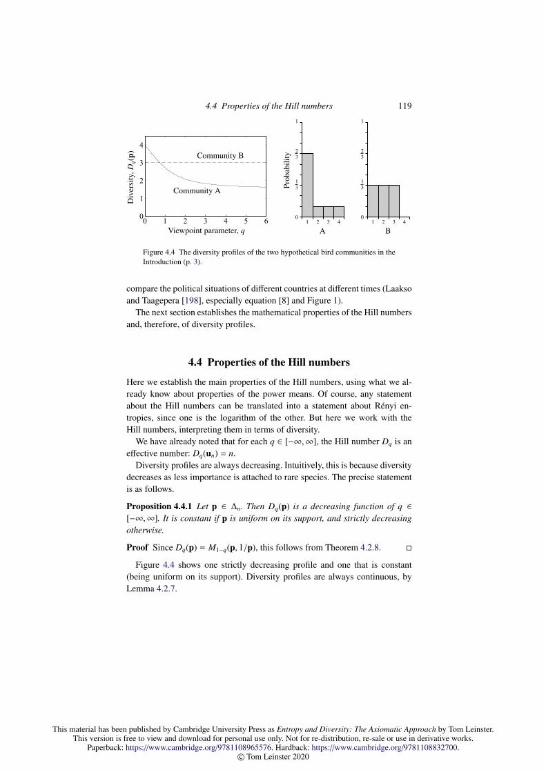
This material has been published by Cambridge University Press as Entropy and Diversity: The Axiomatic Approach by Tom Leinster.This version is free to view and download for personal use only. Not for re-distribution, re-sale or use in derivative works.
Paperback: https://www.cambridge.org/9781108965576. Hardback: https://www.cambridge.org/9781108832700.© Tom Leinster 2020
4.4 Properties of the Hill numbers 119
0
1
2
3
4
0 1 2 3 4 5 6
Community ACommunity B
Community A
Community B
Viewpoint parameter, q
Div
ersi
ty,D
q(p)
Prob
abili
ty
1 2 3 4
A
0
13
23
1
1 2 3 4
B
0
13
23
1
Figure 4.4 The diversity profiles of the two hypothetical bird communities in theIntroduction (p. 3).
compare the political situations of different countries at different times (Laaksoand Taagepera [198], especially equation [8] and Figure 1).
The next section establishes the mathematical properties of the Hill numbersand, therefore, of diversity profiles.
4.4 Properties of the Hill numbers
Here we establish the main properties of the Hill numbers, using what we al-ready know about properties of the power means. Of course, any statementabout the Hill numbers can be translated into a statement about Renyi en-tropies, since one is the logarithm of the other. But here we work with theHill numbers, interpreting them in terms of diversity.
We have already noted that for each q ∈ [−∞,∞], the Hill number Dq is aneffective number: Dq(un) = n.
Diversity profiles are always decreasing. Intuitively, this is because diversitydecreases as less importance is attached to rare species. The precise statementis as follows.
Proposition 4.4.1 Let p ∈ ∆n. Then Dq(p) is a decreasing function of q ∈[−∞,∞]. It is constant if p is uniform on its support, and strictly decreasingotherwise.
Proof Since Dq(p) = M1−q(p, 1/p), this follows from Theorem 4.2.8.
Figure 4.4 shows one strictly decreasing profile and one that is constant(being uniform on its support). Diversity profiles are always continuous, byLemma 4.2.7.
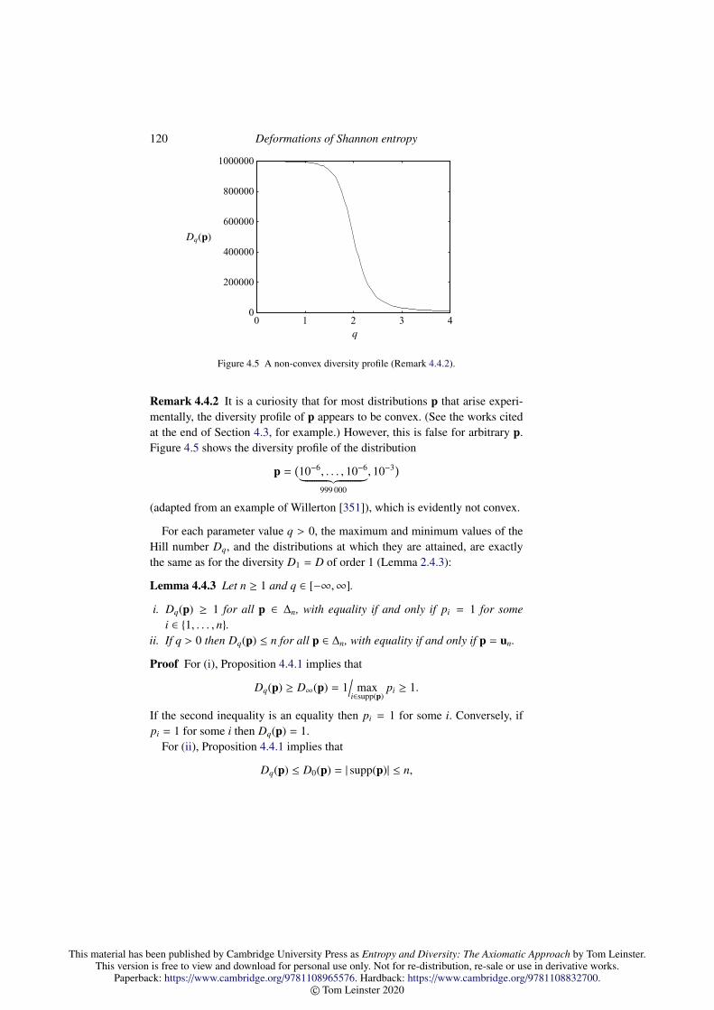
This material has been published by Cambridge University Press as Entropy and Diversity: The Axiomatic Approach by Tom Leinster.This version is free to view and download for personal use only. Not for re-distribution, re-sale or use in derivative works.
Paperback: https://www.cambridge.org/9781108965576. Hardback: https://www.cambridge.org/9781108832700.© Tom Leinster 2020
120 Deformations of Shannon entropy
0
200000
400000
600000
800000
1000000
0 1 2 3 4
q
Dq(p)
Figure 4.5 A non-convex diversity profile (Remark 4.4.2).
Remark 4.4.2 It is a curiosity that for most distributions p that arise experi-mentally, the diversity profile of p appears to be convex. (See the works citedat the end of Section 4.3, for example.) However, this is false for arbitrary p.Figure 4.5 shows the diversity profile of the distribution
p =(10−6, . . . , 10−6︸ ︷︷ ︸
999 000
, 10−3)(adapted from an example of Willerton [351]), which is evidently not convex.
For each parameter value q > 0, the maximum and minimum values of theHill number Dq, and the distributions at which they are attained, are exactlythe same as for the diversity D1 = D of order 1 (Lemma 2.4.3):
Lemma 4.4.3 Let n ≥ 1 and q ∈ [−∞,∞].
i. Dq(p) ≥ 1 for all p ∈ ∆n, with equality if and only if pi = 1 for somei ∈ 1, . . . , n.
ii. If q > 0 then Dq(p) ≤ n for all p ∈ ∆n, with equality if and only if p = un.
Proof For (i), Proposition 4.4.1 implies that
Dq(p) ≥ D∞(p) = 1/
maxi∈supp(p)
pi ≥ 1.
If the second inequality is an equality then pi = 1 for some i. Conversely, ifpi = 1 for some i then Dq(p) = 1.
For (ii), Proposition 4.4.1 implies that
Dq(p) ≤ D0(p) = | supp(p)| ≤ n,

This material has been published by Cambridge University Press as Entropy and Diversity: The Axiomatic Approach by Tom Leinster.This version is free to view and download for personal use only. Not for re-distribution, re-sale or use in derivative works.
Paperback: https://www.cambridge.org/9781108965576. Hardback: https://www.cambridge.org/9781108832700.© Tom Leinster 2020
4.4 Properties of the Hill numbers 121
with equality in the first inequality if and only if p is uniform on its support.On the other hand, equality holds in the second inequality if and only if p hasfull support. Hence equality holds throughout if and only if p = un.
Remarks 4.4.4 i. It follows that for q > 0, the Renyi entropy Hq(p) is mini-mized exactly when p is of the form (0, . . . , 0, 1, 0, . . . , 0), with value 0, andmaximized exactly when p = un, with value log n. Since the q-logarithmicentropy S q(p) is an increasing invertible transformation of Hq(p) (equa-tions (4.18) and (4.19)), it is minimized and maximized at these same dis-tributions, with minimum 0 and maximum S q(un) = lnq(n).
ii. The Hill numbers of negative orders are not maximized by the uniform dis-tribution. Indeed, let q < 0, let n ≥ 2, and take any non-uniform distributionp ∈ ∆n of full support. Then D0(p) = | supp(p)| = n, and the diversityprofile of p is strictly decreasing by Proposition 4.4.1, so
Dq(p) > D0(p) = n = Dq(un).
Whatever the word ‘diverse’ should mean, it is generally agreed that themost diverse abundance distribution on a given set of species should be theuniform distribution. (At least, this should be the case for the crude modelof a community as a probability distribution, which we are using here. Seealso Section 6.3.) For this reason, the Hill numbers of negative orders aregenerally not used as measures of diversity.
On the other hand, the Hill numbers of negative orders measure some-thing. For instance,
D−∞(p) = 1/
mini∈supp(p)
pi = maxi∈supp(p)
(1/pi)
measures the rarity of the rarest species, giving a high value to any commu-nity containing at least one species that is very rare. This is a meaningfulquantity, even if it should not be called diversity.
We now show that the Hill number Dq(p) of a given order q is very nearlycontinuous in p ∈ ∆n, with the sole exception that Dq is discontinuous at theboundary of the simplex when q ≤ 0. For instance, species richness D0 isdiscontinuous: in terms of the number of species present, a relative abundanceof 0.0001 is qualitatively different from a relative abundance of 0.
Definition 4.4.5 Let(D : ∆n → (0,∞)
)n≥1 be a sequence of functions. Then D
is continuous if the function D : ∆n → (0,∞) is continuous for each n ≥ 1,and continuous in positive probabilities if the restriction D|∆n of D to theopen simplex is continuous for each n ≥ 1.

This material has been published by Cambridge University Press as Entropy and Diversity: The Axiomatic Approach by Tom Leinster.This version is free to view and download for personal use only. Not for re-distribution, re-sale or use in derivative works.
Paperback: https://www.cambridge.org/9781108965576. Hardback: https://www.cambridge.org/9781108832700.© Tom Leinster 2020
122 Deformations of Shannon entropy
Continuity in positive probabilities means that small changes to the abun-dances of the species present cause only small changes in the perceived diver-sity. For example, D0 is continuous in positive probabilities, even though it isnot continuous.
Lemma 4.4.6 i. For each q ∈ [−∞,∞], the Hill number Dq is continuous inpositive probabilities.
ii. For each q ∈ (0,∞], the Hill number Dq is continuous.
Proof Part (i) is immediate from the explicit formulas for Dq (equations(4.21)–(4.24)), and part (ii) follows from the observation that when q > 0,the formulas for Dq are unchanged if we allow i to range over all of 1, . . . , ninstead of just supp(p).
Next we establish the algebraic properties of the Hill numbers, beginningwith the most elementary ones.
Definition 4.4.7 A sequence of functions(D : ∆n → (0,∞)
)n≥1 is absence-
invariant if whenever p ∈ ∆n and 1 ≤ i ≤ n with pi = 0, then
D(p) = D(p1, . . . , pi−1, pi+1, . . . , pn).
Absence-invariance means that as far as D is concerned, a species that isabsent might as well not have been mentioned.
Recall from equation (4.4) that D is said to be symmetric if D(pσ) = D(p)for all p ∈ ∆n and permutations σ of 1, . . . , n. This means that the diversityis unaffected by the order in which the species happen to be listed.
Lemma 4.4.8 For each q ∈ [−∞,∞], the Hill number Dq of order q is sym-metric and absence-invariant.
Proof These statements follow from the symmetry and absence-invariance ofthe power means (Lemma 4.2.11). Alternatively, they can be deduced directlyfrom the explicit formulas for Dq (equations (4.21)–(4.24)).
Remark 4.4.9 By symmetry, p and pσ have the same diversity profile. In fact,the converse also holds: if p, r ∈ ∆n have the same diversity profile then p andr must be the same up to a permutation. This is proved in Appendix A.3.
Thus, the diversity profile of a relative abundance distribution contains allthe information about that distribution apart from which species is which,packaged in a way that displays meaningful information about the commu-nity’s diversity.

This material has been published by Cambridge University Press as Entropy and Diversity: The Axiomatic Approach by Tom Leinster.This version is free to view and download for personal use only. Not for re-distribution, re-sale or use in derivative works.
Paperback: https://www.cambridge.org/9781108965576. Hardback: https://www.cambridge.org/9781108832700.© Tom Leinster 2020
4.4 Properties of the Hill numbers 123
We finally come to the chain rule. In Corollary 2.4.8, we treated the caseq = 1, showing that
D1(w (p1, . . . ,pn)
)= D1(w) ·
n∏i=1
D1(pi)wi
for all w ∈ ∆n and pi ∈ ∆ki . In Example 2.4.9, this formula was explained interms of a group of n islands of relative sizes wi and diversities di = D1(pi),with no shared species. We now give the chain rule for general q, in two dif-ferent forms.
Proposition 4.4.10 (Chain rule, version 1) Let q ∈ [−∞,∞], w ∈ ∆n, andp1 ∈ ∆k1 , . . . ,pn ∈ ∆kn . Write di = Dq(pi) and d = (d1, . . . , dn). Then
Dq(w (p1, . . . ,pn)
)= M1−q(w,d/w)
=
(∑wq
i d1−qi
)1/(1−q) if q , 1,±∞,
max di/wi if q = −∞,∏(di/wi)wi if q = 1,
min di/wi if q = ∞,
where the sum, maximum, product, and minimum are over i ∈ supp(w).
Here d/w = (d1/w1, . . . , dn/wn), as in Remark 4.2.9.
Proof We have
Dq(w (p1, . . . ,pn)
)= M1−q
(w (p1, . . . ,pn), 1
w1p1 ⊕ · · · ⊕1
wnpn
)= M1−q
(w,
(M1−q
(p1, 1
w1p1
), . . . , M1−q
(pn, 1
wnpn
)))= M1−q
(w, (d1/w1, . . . , dn/wn)
),
where the second equation follows from the chain rule for M1−q (Proposi-tion 4.2.24) and the last from the homogeneity of M1−q (Lemma 4.2.22). Thisproves the first equality stated in the proposition, and the second follows fromthe explicit formulas for the power means.
There is an alternative form of the chain rule, for which we will need someterminology. Given a probability distribution w ∈ ∆n and a real number q,the escort distribution of order q of w is the distribution w(q) ∈ ∆n with ithcoordinate
w(q)i =
wq
i
/ ∑j∈supp(w)
wqj if i ∈ supp(w),
0 otherwise.

This material has been published by Cambridge University Press as Entropy and Diversity: The Axiomatic Approach by Tom Leinster.This version is free to view and download for personal use only. Not for re-distribution, re-sale or use in derivative works.
Paperback: https://www.cambridge.org/9781108965576. Hardback: https://www.cambridge.org/9781108832700.© Tom Leinster 2020
124 Deformations of Shannon entropy
Lemma 4.4.11 Let q ∈ R, w ∈ ∆n, and d ∈ [0,∞)n. Then
M1−q(w,d/w) = Dq(w) · M1−q(w(q),d).
Proof For the case q = 1, note that
M0(w, xy) = M0(w, x)M0(w, y)
for all x, y ∈ [0,∞)n. It follows that
D1(w) · M0(w(1),d) = M0(w, 1/w) · M0(w,d) = M0(w,d/w).
On the other hand, for 1 , q ∈ R,
M1−q(w,d/w) =
( ∑i∈supp(w)
wqi d1−q
i
)1/(1−q)
= Dq(w) ·(∑
i∈supp(w) wqi d1−q
i∑j∈supp(w) wq
j
)1/(1−q)
= Dq(w) · M1−q(w(q),d),
as required.
The last two results immediately imply:
Proposition 4.4.12 (Chain rule, version 2) Let q ∈ R, w ∈ ∆n, and p1 ∈
∆k1 , . . . ,pn ∈ ∆kn . Write di = Dq(pi) and d = (d1, . . . , dn). Then
Dq(w (p1, . . . ,pn)
)= Dq(w) · M1−q(w(q),d).
Remarks 4.4.13 Here we provide context for the notion of escort distribution.
i. The escort distributions of a distribution w form a one-parameter family(w(q))
q∈R
of distributions, of which the original distribution w is the member corre-sponding to q = 1. The term ‘escort distribution’ is taken from thermody-namics (Chapter 9 of Beck and Schlogl [33]). There, one encounters ex-pressions such as
(e−βE1 , . . . , e−βEn )Z(β)
,
where Z(β) = e−βE1 + · · · + e−βEn is the partition function for energies Ei atinverse temperature β. Assuming without loss of generality that
∑e−Ei = 1,
the inverse temperature β plays the role of the parameter q.

This material has been published by Cambridge University Press as Entropy and Diversity: The Axiomatic Approach by Tom Leinster.This version is free to view and download for personal use only. Not for re-distribution, re-sale or use in derivative works.
Paperback: https://www.cambridge.org/9781108965576. Hardback: https://www.cambridge.org/9781108832700.© Tom Leinster 2020
4.4 Properties of the Hill numbers 125
Figure 4.6 Twelve one-dimensional linear subspaces of the open simplex ∆3 withthe real vector space structure described in Remark 4.4.13(ii).
ii. The function (q,w) 7→ w(q) is the scalar multiplication of a real vector spacestructure on the interior ∆n of the simplex. Addition is given by
(p, r) 7→(p1r1, . . . , pnrn)p1r1 + · · · + pnrn
,
and the zero element is the uniform distribution un. Figure 4.6 shows someone-dimensional linear subspaces of the two-dimensional vector space ∆3.This vector space structure was used in the field of statistical inference byAitchison [5], and is sometimes named after him. It can be understood al-gebraically as follows.
Exponential and logarithm define a bijection between R and (0,∞). Thisinduces a bijection between Rn and (0,∞)n, and transporting the vectorspace structure on Rn across this bijection gives a vector space structureon (0,∞)n. Explicitly, addition in the vector space (0,∞)n is coordinate-wise multiplication, the zero element is (1, . . . , 1), and scalar multiplicationby q ∈ R raises each coordinate to the power of q.
Now take the linear subspace of Rn spanned by (1, . . . , 1). The corre-sponding subspace W of (0,∞)n is (γ, . . . , γ) : γ ∈ (0,∞), and we canform the quotient vector space (0,∞)n/W.
An element of this quotient is an equivalence class of vectors y ∈ (0,∞)n,with y equivalent to z if and only if y = γz for some γ > 0. Geometrically,then, the equivalence classes are the rays through the origin in the positiveorthant (0,∞)n. Each ray contains exactly one element of the open simplex
∆n = y ∈ (0,∞)n : y1 + · · · + yn = 1.

This material has been published by Cambridge University Press as Entropy and Diversity: The Axiomatic Approach by Tom Leinster.This version is free to view and download for personal use only. Not for re-distribution, re-sale or use in derivative works.
Paperback: https://www.cambridge.org/9781108965576. Hardback: https://www.cambridge.org/9781108832700.© Tom Leinster 2020
126 Deformations of Shannon entropy
This puts (0,∞)n/W in bijection with ∆n, thus giving ∆n the structure ofa vector space. It is exactly the vector space structure defined explicitlyabove.
iii. In statistical language, each linear subspace of the vector space ∆n is anexponential family of distributions on 1, . . . , n. For example, the one-dimensional subspace spanned by p ∈ ∆n is a one-parameter exponen-tial family with natural parameter q ∈ R, sufficient statistic log pi, andlog-partition function log
(∑pq
i). More on this connection can be found in
Amari [10], Ay, Jost, Le and Schwachhofer ([22], Section 2.8), and otherinformation geometry texts.
As already discussed in the case q = 1 (Example 2.4.9), the chain rule forthe Hill numbers has the important consequence that when computing the totaldiversity of a group of islands with no shared species, the only informationone needs is the diversities and relative sizes of the islands, not their internalmake-up:
Definition 4.4.14 A sequence of functions(D : ∆n → (0,∞)
)n≥1 is modular
if
D(pi) = D
(pi) for all i ∈ 1, . . . , n
=⇒ D(w (p1, . . . ,pn)
)= D
(w (p1, . . . , pn)
)for all n, k1, . . . , kn, k1, . . . , kn ≥ 1 and w ∈ ∆n, pi ∈ ∆ki , pi ∈ ∆ki
.
In other words, D is modular if D(w (p1, . . . ,pn)
)depends only on w and
D(p1), . . . ,D(pn).
Corollary 4.4.15 (Modularity) For each q ∈ [−∞,∞], the Hill number Dq ismodular.
The chain rule has two further consequences.
Definition 4.4.16 A sequence of functions(D : ∆n → (0,∞)
)n≥1 is multi-
plicative if
D(p ⊗ r) = D(p)D(r)
for all m, n ≥ 1, p ∈ ∆m, and r ∈ ∆n.
Corollary 4.4.17 (Multiplicativity) For each q ∈ [−∞,∞], the Hill numberDq is multiplicative.
Proof This follows from either the chain rule for the Hill numbers or the log-arithmic property of the Renyi entropies (equation (4.14)).

This material has been published by Cambridge University Press as Entropy and Diversity: The Axiomatic Approach by Tom Leinster.This version is free to view and download for personal use only. Not for re-distribution, re-sale or use in derivative works.
Paperback: https://www.cambridge.org/9781108965576. Hardback: https://www.cambridge.org/9781108832700.© Tom Leinster 2020
4.5 Characterization of the Hill number of a given order 127
Definition 4.4.18 A sequence of functions(D : ∆n → (0,∞)
)n≥1 satisfies the
replication principle if
D(un ⊗ p) = nD(p)
for all n, k ≥ 1 and p ∈ ∆k.
The oil company argument of Example 2.4.11 shows the fundamental im-portance of the replication principle. If n islands have the same relative abun-dance distribution p, but on disjoint sets of species, the diversity of the wholesystem should be nD(p).
Corollary 4.4.19 (Replication) For each q ∈ [−∞,∞], the Hill number Dq
satisfies the replication principle.
Proof This follows from multiplicativity and the fact that Dq is an effectivenumber.
Accompanying the Renyi entropies, there is also a notion of Renyi relativeentropy (introduced in Section 3 of Renyi [291]). We defer discussion to Sec-tion 7.2.
4.5 Characterization of the Hill number of a given order
In this book, we prove two characterization theorems for the Hill numbers.The first states that for each given q, the unique function satisfying certainconditions (which depend on q) is Dq. The second states that the only functionssatisfying a different list of conditions (which make no mention of q) are thosebelonging to the family (Dq)q∈[−∞,∞]. We prove the first characterization in thissection, and the second in Section 7.4.
For the q-logarithmic entropies, we have already proved an analogue of thefirst result (Theorem 4.1.5). We will not prove an analogue of the second. How-ever, there is a theorem of this type due to Forte and Ng, briefly discussed inRemark 7.4.15.
Here we build on work of Routledge [299] to characterize the Hill numberDq for each given q ∈ (0,∞). The restriction to positive q ensures that Dq iscontinuous on all of ∆n (by Lemma 4.4.6(ii)).
Recall that Dq satisfies the chain rule
Dq(w (p1, . . . ,pn)
)= Dq(w) · M1−q
(w(q),
(Dq(p1), . . . ,Dq(pn)
)), (4.26)
where w ∈ ∆n and pi ∈ ∆ki (Proposition 4.4.12). Let us reflect on equa-tion (4.26), interpreting it in terms of the island scenario of Examples 2.1.6
This material has been published by Cambridge University Press as Entropy and Diversity: The Axiomatic Approach by Tom Leinster.This version is free to view and download for personal use only. Not for re-distribution, re-sale or use in derivative works.
Paperback: https://www.cambridge.org/9781108965576. Hardback: https://www.cambridge.org/9781108832700.© Tom Leinster 2020
128 Deformations of Shannon entropy
and 2.4.9. Equation (4.26) can be interpreted as a decomposition of the di-versity of the island group into two factors: the variation between the islands(given by Dq(w)), and the average variation or diversity within the islands(given by the second factor). Recall that in the island scenario, there is nooverlap of species between islands, so the variation between the islands de-pends only on the variation in sizes.
Now, suppose that we want to list some properties that a reasonable diver-sity measure D ought to satisfy. One such property might be that D is de-composable in the sense just described: D(w (p1, . . . ,pn)) is equal to thevariation D(w) between islands multiplied by the average of the diversitiesD(p1), . . . ,D(pn) within each island.
But what could ‘average’ reasonably mean? We have already seen that thepower means have many good properties that we would expect of a notion ofavarage, and we will see in Chapter 5 that in a certain precise sense, they areuniquely good. So, it is reasonable to take the ‘average’ to be some power meanMt, and we can make the usual harmless reparametrization t = 1 − q.
This reasoning suggests that our hypothetical diversity measure D shouldsatisfy something like equation (4.26), with D in place of Dq. Still, it does notexplain why the average of the within-island diversities should be calculatedusing the weighting w(q) on the islands, rather than some other weighting. Allthat seems clear is that the weighting should depend on the sizes of the is-lands only. If we write the weighting as θ(w), then our conclusion is that anyreasonable diversity measure D ought to satisfy the equation
D(w (p1, . . . ,pn)
)= D(w) · M1−q
(θ(w),
(D(p1), . . . ,D(pn)
))for some q and some function θ : ∆n → ∆n. This explains the most substantialof the hypotheses in our main result:
Theorem 4.5.1 Let q ∈ (0,∞). Let(D : ∆n → (0,∞)
)n≥1 be a sequence of
functions. The following are equivalent:
i. the functions D are continuous, symmetric and effective numbers, and foreach n ≥ 1 there exists a function θ : ∆n → ∆n with the following property:
D(w (p1, . . . ,pn)
)= D(w) · M1−q
(θ(w),
(D(p1), . . . ,D(pn)
))for all w ∈ ∆n, k1, . . . , kn ≥ 1, and pi ∈ ∆ki ;
ii. D = Dq.
Theorem 4.5.1 is a variation on a 1979 result of Routledge (Theorem 1 ofthe appendix to [299]).
This material has been published by Cambridge University Press as Entropy and Diversity: The Axiomatic Approach by Tom Leinster.This version is free to view and download for personal use only. Not for re-distribution, re-sale or use in derivative works.
Paperback: https://www.cambridge.org/9781108965576. Hardback: https://www.cambridge.org/9781108832700.© Tom Leinster 2020
4.5 Characterization of the Hill number of a given order 129
The rest of this section is devoted to the proof. We already showed in Sec-tion 4.4 that (ii) implies (i). Conversely, and for the rest of this section, takeD and θ satisfying the conditions of (i). By the standard abuse of notation, weuse the same letter θ for each of the functions θ : ∆1 → ∆1, θ : ∆2 → ∆2, etc.We have to prove that D = Dq.
For p ∈ ∆n, write
θ(p) =(θ1(p), . . . , θn(p)
).
Our first lemma shows how θ1 can be expressed in terms of D. We temporarilyadopt the notation
p# = p (u2,u1, . . . ,u1) =( 1
2 p1,12 p1, p2, . . . , pn
)(p ∈ ∆n).
Lemma 4.5.2 For all n ≥ 1 and p ∈ ∆n,
θ1(p) =1
lnq 2· lnq
D(p#)D(p)
.
Proof By the main hypothesis on D and the effective number property,
D(p#) = D(p) · M1−q(θ(p), (2, 1, . . . , 1)
).
Hence by Lemma 4.2.29,
lnqD(p#)D(p)
= M1(θ(p), (lnq 2, lnq 1, . . . , lnq 1)
).
But lnq 1 = 0, so the right-hand side is just θ1(p) lnq 2.
We use this lemma to compute the weighting θ(w (p1, . . . ,pn)) of a com-posite distribution:
Lemma 4.5.3 Let w ∈ ∆n and p1 ∈ ∆k1 , . . . ,pn ∈ ∆kn . Then
θ1(w (p1, . . . ,pn)
)=
θ1(w)D(p1)1−q∑ni=1 θi(w)D(pi)1−q θ1(p1).
This material has been published by Cambridge University Press as Entropy and Diversity: The Axiomatic Approach by Tom Leinster.This version is free to view and download for personal use only. Not for re-distribution, re-sale or use in derivative works.
Paperback: https://www.cambridge.org/9781108965576. Hardback: https://www.cambridge.org/9781108832700.© Tom Leinster 2020
130 Deformations of Shannon entropy
Proof Write di = D(pi) and d#1 = D
(p1#). We have
θ1(w (p1, . . . ,pn)
)=
1lnq 2
· lnq
D((
w (p1, . . . ,pn))#)
D(w (p1, . . . ,pn)
) (4.27)
=1
lnq 2· lnq
D(w
(p1#
,p2, . . . ,pn))
D(w (p1,p2, . . . ,pn)
) (4.28)
=1
lnq 2· lnq
M1−q(θ(w), (d#
1 , d2, . . . , dn))
M1−q(θ(w), (d1, d2, . . . , dn)
) (4.29)
=1
lnq 2·
lnq M1−q(θ(w), (d#
1 , d2, . . . , dn))− lnq M1−q
(θ(w), (d1, d2, . . . , dn)
)M1−q
(θ(w), (d1, d2, . . . , dn)
)1−q
(4.30)
=1
lnq 2·
M1(θ(w), (lnq d#
1 , lnq d2, . . .))− M1
(θ(w), (lnq d1, lnq d2, . . .)
)∑ni=1 θi(w)d1−q
i(4.31)
=1
lnq 2·θ1(w)(lnq d#
1 − lnq d1)∑ni=1 θi(w)d1−q
i
(4.32)
=1
lnq 2·
θ1(w)d1−q1∑n
i=1 θi(w)d1−qi
· lnqd#
1
d1(4.33)
=θ1(w)d1−q
1∑ni=1 θi(w)d1−q
i
· θ1(p1), (4.34)
where equations (4.27) and (4.34) follow from Lemma 4.5.2, equation (4.28)from the definition of #, equation (4.29) from the main hypothesis on D, equa-tions (4.30) and (4.33) from the quotient formula
lnqxy
=lnq x − lnq y
y1−q
for the q-logarithm (equation (1.20)), equation (4.31) from Lemma 4.2.29 andthe definition of M1−q, and equation (4.32) from the definition of the arithmeticmean M1.
We now deduce that the weightings must be the q-escort distributions:
Lemma 4.5.4 θ(w) = w(q) for all n ≥ 1 and w ∈ ∆n.
Proof Following a familiar pattern, we prove this first when w is uniform, thenwhen the coordinates of w are positive and rational, and finally for arbitrary w.
This material has been published by Cambridge University Press as Entropy and Diversity: The Axiomatic Approach by Tom Leinster.This version is free to view and download for personal use only. Not for re-distribution, re-sale or use in derivative works.
Paperback: https://www.cambridge.org/9781108965576. Hardback: https://www.cambridge.org/9781108832700.© Tom Leinster 2020
4.5 Characterization of the Hill number of a given order 131
For the case w = un, we have to prove that θ(un) = un. By Lemma 4.5.2,
θ1(un) =1
lnq 2lnq
D(un (u2,u1,u1, . . . ,u1)
)D(un)
,
and by the same argument,
θ2(un) =1
lnq 2lnq
D(un (u1,u2,u1, . . . ,u1)
)D(un)
.
By symmetry of D, the right-hand sides of these two equations are equal.Hence θ1(un) = θ2(un). Similarly, θi(un) = θ j(un) for all i, j, and so θ(un) = un.
Now let w ∈ ∆n with
w = (k1/k, . . . , kn/k)
for some positive integers ki, where k =∑
ki. We have
w (uk1 , . . . ,ukn ) = uk. (4.35)
Applying θ1 to both sides gives
θ1(w)k1−q1∑
θi(w)k1−qi
1k1
=1k,
using Lemma 4.5.3, the effective number property of D, and the previous para-graph. This rearranges to
θ1(w) = wq1
n∑i=1
θi(w)w1−qi .
By the same argument,
θ j(w) = wqj
n∑i=1
θi(w)w1−qi
for all j = 1, . . . , n. The sum on the right-hand side is independent of j, so θ(w)is a probability distribution proportional to
(wq
1, . . . ,wqn), forcing θ(w) = w(q).
Finally, we show that θ(w) = w(q) for all w ∈ ∆n. By Lemma 4.5.2 andthe continuity hypothesis on D, the map θ1 is continuous, and similarly forθ2, . . . , θn. Hence θ : ∆n → ∆n is continuous. So too is the map w 7→ w(q).But by the previous paragraph, these last two maps are equal on the positiverational distributions, so they are equal everywhere.
Proof of Theorem 4.5.1 First, consider distributions w = (k1/k, . . . , kn/k)with positive rational coordinates. Apply D to both sides of equation (4.35):then by Lemma 4.5.4 and the effective number hypothesis on D,
D(w) · M(w(q), (k1, . . . , kn)
)= k.

This material has been published by Cambridge University Press as Entropy and Diversity: The Axiomatic Approach by Tom Leinster.This version is free to view and download for personal use only. Not for re-distribution, re-sale or use in derivative works.
Paperback: https://www.cambridge.org/9781108965576. Hardback: https://www.cambridge.org/9781108832700.© Tom Leinster 2020
132 Deformations of Shannon entropy
But we can also apply Dq to both sides of equation (4.35): then by the chainrule and the effective number property of Dq,
Dq(w) · M(w(q), (k1, . . . , kn)
)= k.
Hence D(w) = Dq(w). And by the continuity hypothesis on D and the conti-nuity property of Dq (Lemma 4.4.6(ii)), it follows that D(w) = Dq(w) for allw ∈ ∆n.

This material has been published by Cambridge University Press as Entropy and Diversity: The Axiomatic Approach by Tom Leinster.This version is free to view and download for personal use only. Not for re-distribution, re-sale or use in derivative works.
Paperback: https://www.cambridge.org/9781108965576. Hardback: https://www.cambridge.org/9781108832700.© Tom Leinster 2020
5
Means
The ideal of the axiomatic approach to diversity measurement is to be able tosay ‘any measure of diversity that satisfies properties X, Y and Z must be oneof the following.’ Our later theorems of this type will stand on the shoulders ofcharacterization theorems for means.
The theory of means took shape in the first half of the twentieth century,with the 1930 papers of Kolmogorov [190, 192] and Nagumo [257] as well asHardy, Littlewood and Polya’s seminal book Inequalities [135], first publishedin 1934. (Aczel [1] describes the early history.) But new results continue tobe proved. The 2009 book by Grabisch, Marichal, Mesiar and Pap lists somemodern developments ([124], Chapter 4), and most of the characterization the-orems in this chapter also appear to be new.
The arguments that we will use are entirely elementary and require no spe-cialist knowledge. Nevertheless, the reader could omit almost all of this chap-ter without affecting their ability to follow subsequent chapters. The only partsneeded later are the statements of Theorems 5.5.10 and 5.5.11.
Compared to most of the literature on characterizations of means, the resultsand proofs in this chapter have a particular flavour. First, we are mainly inter-ested in the power means, as opposed to the much larger class of quasiarithme-tic means (defined below). That makes it reasonable to assume a homogeneityaxiom, which in turn means that we can almost always do without continu-ity. (The absence of continuity hypotheses distinguishes our results from manyothers, such as those of Fodor and Marichal [105].) Second, we wish to includethe end cases M∞ = max and M−∞ = min of the power means, and the factthat these means are not strictly increasing alters considerably the argumentsthat can be used.
A key role is played by what Tao calls the ‘tensor power trick’ ([322], Sec-tion 1.9), which can be described as follows. Take a set X and two functionsF,G : X → R+. Suppose we want to prove that F ≤ G, but have only been
133

This material has been published by Cambridge University Press as Entropy and Diversity: The Axiomatic Approach by Tom Leinster.This version is free to view and download for personal use only. Not for re-distribution, re-sale or use in derivative works.
Paperback: https://www.cambridge.org/9781108965576. Hardback: https://www.cambridge.org/9781108832700.© Tom Leinster 2020
134 Means
strictly increasing increasing
(0,∞) t ∈ (−∞,∞) t ∈ [−∞,∞]Theorem 5.3.2 Theorem 5.4.7
[0,∞) t ∈ (0,∞) t ∈ [−∞,∞]Theorem 5.3.3 Theorem 5.4.9
(also assume continuous and nonzero)
Table 5.1 Summary of characterization theorems for symmetric, decomposable,homogeneous, unweighted means. For instance, the top-left entry indicates thatthe strictly increasing such means on (0,∞) are exactly the unweighted powermeans Mt of order t ∈ (−∞,∞). Table 5.2 (p. 162) gives the corresponding resultson weighted means.
able to find a constant C (perhaps large) such that F ≤ CG. In general, there isnothing more to be said. However, suppose now that X can be equipped with aproduct that is preserved by both F and G. Let x ∈ X. Then for all n ≥ 1,
F(x) = F(xn)1/n ≤ (CG(xn))1/n = C1/nG(x),
and letting n→ ∞ gives F(x) ≤ G(x), as desired.Trivial as it may seem, the tensor power trick can be wielded to powerful
effect. Typically X is taken to be a set of vectors or functions equipped withthe tensor product. Tao [322] demonstrates the tensor power trick by using itto prove the Hausdorff–Young inequality, and notes that it also plays a partin Deligne’s proof of the Weil conjectures. We will use it in the proof of thepivotal Lemma 5.4.3.
This chapter begins with the classical theory of quasiarithmetic means,which are just ordinary arithmetic means transported along a homeomorphism(Section 5.1). The bulk of the chapter (Sections 5.2–5.4) concerns general un-weighted means, and culminates in the four characterization theorems shownin Table 5.1.
Finally, in Section 5.5, we develop a method for converting characterizationtheorems for unweighted means into characterization theorems for weightedmeans. This method is applied to the four theorems just mentioned. One ofthe resulting four characterizations of weighted means goes back to Hardy,Littlewood and Polya in 1934, while the others may be new.
We will be defining a considerable amount of terminology for properties ofmeans. Appendix B contains a summary for convenient reference. The word‘mean’ in isolation will be used informally, without precise definition.

This material has been published by Cambridge University Press as Entropy and Diversity: The Axiomatic Approach by Tom Leinster.This version is free to view and download for personal use only. Not for re-distribution, re-sale or use in derivative works.
Paperback: https://www.cambridge.org/9781108965576. Hardback: https://www.cambridge.org/9781108832700.© Tom Leinster 2020
5.1 Quasiarithmetic means 135
5.1 Quasiarithmetic means
Let J be a real interval. The arithmetic mean defines a sequence of functions(M1 : ∆n × Jn → J
)n≥1.
For any other set I and bijection φ : I → J, we can transport the arithmeticmean on J along φ to obtain a kind of mean on I. We will focus on the casewhere I is also an interval and φ is a homeomorphism (that is, both φ and φ−1
are continuous), as follows.
Definition 5.1.1 Let φ : I → J be a homeomorphism between real intervals.The quasiarithmetic mean on I generated by φ is the sequence of functions(
Mφ : ∆n × In → I)n≥1
defined by
Mφ(p, x) = φ−1( n∑
i=1
piφ(xi))
(p ∈ ∆n, x ∈ In).
The theory of quasiarithmetic means is classical, and most of the contentof this section can be found, more or less explicitly, in Chapter III of Hardy,Littlewood and Polya [135].
Remark 5.1.2 In the literature, the terms ‘quasiarithmetic’ and ‘quasilinear’are both used, sometimes interchangeably, sometimes with the former reservedfor the unweighted case, and sometimes with the latter meaning what we callmodularity (Definition 4.2.25). ‘Quasiarithmetic’ has the advantage of evokingthe fact that a quasiarithmetic mean is just an arithmetic mean disguised by achange of variable: the diagram
∆n × In Mφ //
1×φn
I
φ
∆n × Jn
M1
// J
commutes.
Example 5.1.3 For real t , 0, the power mean Mt on (0,∞) is the quasi-arithmetic mean Mφt generated by the homeomorphism
φt : (0,∞) → (0,∞)t 7→ xt.

This material has been published by Cambridge University Press as Entropy and Diversity: The Axiomatic Approach by Tom Leinster.This version is free to view and download for personal use only. Not for re-distribution, re-sale or use in derivative works.
Paperback: https://www.cambridge.org/9781108965576. Hardback: https://www.cambridge.org/9781108832700.© Tom Leinster 2020
136 Means
The geometric mean M0 on (0,∞) is the quasiarithmetic mean Mφ0 generatedby the homeomorphism
φ0 = log : (0,∞)→ R.
Thus, all the power means of finite order on (0,∞) are quasiarithmetic.
Example 5.1.4 The power means M±∞ on (0,∞) are not quasiarithmetic, aswe will prove in Example 5.2.8(i).
Example 5.1.5 The quasiarithmetic mean on R generated by the homeomor-phism exp: R→ (0,∞) is given by
Mexp(p, x) = log( n∑
i=1
piexi
)(p ∈ ∆n, x ∈ Rn). This is the exponential mean, whose special propertieswere established by Nagumo ([257], p. 78; or for a modern account, see The-orem 4.15(i) of Grabisch, Marichal, Mesiar and Pap [124]).
The rest of this section is dedicated to three questions.First, when do two homeomorphisms out of an interval I generate the same
quasiarithmetic mean on I?Second, among all quasiarithmetic means on (0,∞), how can we pick out
the power means Mt (t ∈ R)? In other words, what special properties do thepower means possess?
Third (and imprecisely for now), given a mean on some large interval, if itsrestrictions to smaller intervals are quasiarithmetic, is it quasiarithmetic itself?
The answers to all three questions involve the notion of affine map.
Definition 5.1.6 Let I be a real interval. A function α : I → R is affine if
α(px1 + (1 − p)x2
)= pα(x1) + (1 − p)α(x2)
for all x1, x2 ∈ I and p ∈ [0, 1].
Lemma 5.1.7 Let α : I → J be a function between real intervals. The follow-ing are equivalent:
i. α is affine;ii. α
(∑λixi
)=
∑λiα(xi) for all n ≥ 1, x1, . . . , xn ∈ I and λ1, . . . , λn ∈ R such
that∑λi = 1 and
∑λixi ∈ I;
iii. there exist constants a, b ∈ R such that α(x) = ax + b for all x ∈ I;iv. α is continuous and α
( 12 (x1 + x2)
)= 1
2(α(x1) + α(x2)
)for all x1, x2 ∈ I.
Note that in (ii), some of the coefficients λi may be negative.

This material has been published by Cambridge University Press as Entropy and Diversity: The Axiomatic Approach by Tom Leinster.This version is free to view and download for personal use only. Not for re-distribution, re-sale or use in derivative works.
Paperback: https://www.cambridge.org/9781108965576. Hardback: https://www.cambridge.org/9781108832700.© Tom Leinster 2020
5.1 Quasiarithmetic means 137
Proof See Appendix A.4.
By part (iii), any affine map is either injective or constant. We will needthe following elementary observation on extension of affine maps to largerdomains.
Definition 5.1.8 A real interval is trivial if it has at most one element, andnontrivial otherwise.
Lemma 5.1.9 Let I ⊆ J be real intervals and let α : I → R be an affine map.Then:
i. there exists an affine map α : J → R extending α;ii. if α is injective then we may choose α to be injective;
iii. if I is nontrivial then α is uniquely determined by α.
Proof Choose a, b ∈ R such that α(x) = ax + b for all x ∈ I. For (i), putα(y) = ay + b for y ∈ J. For (ii), if α is injective then we can choose a to benonzero, so α is injective. Part (iii) is trivial.
We are now ready to answer the first question: when are two quasiarithmeticmeans equal?
Proposition 5.1.10 Let
J
I
φ 77
φ′ '' J′
be homeomorphisms between real intervals. The following are equivalent:
i. Mφ = Mφ′ : ∆n × In → I for all n ≥ 1;ii. Mφ(un,−) = Mφ′ (un,−) : In → I for all n ≥ 1;
iii. the map φ′ φ−1 : J → J′ is affine.
This is Theorem 83 of the book [135] by Hardy, Littlewood and Polya, whoattribute it to Jessen and Knopp.
Proof Trivially, (i) implies (ii).Assuming (ii), we prove (iii). Write α = φ′ φ−1. We will prove that α is
affine using Lemma 5.1.7(iv). Certainly α is continuous. Now let y1, y2 ∈ J.We have
Mφ
(u2,
(φ−1(y1), φ−1(y2)
))= Mφ′
(u2,
(φ−1(y1), φ−1(y2)
)),

This material has been published by Cambridge University Press as Entropy and Diversity: The Axiomatic Approach by Tom Leinster.This version is free to view and download for personal use only. Not for re-distribution, re-sale or use in derivative works.
Paperback: https://www.cambridge.org/9781108965576. Hardback: https://www.cambridge.org/9781108832700.© Tom Leinster 2020
138 Means
or explicitly,
φ−1( 12 y1 + 1
2 y2)
= φ′−1( 12φ′φ−1(y1) + 1
2φ′φ−1(y2)
).
But this can be rewritten as
α( 1
2 (y1 + y2))
= 12(α(y1) + α(y2)
),
so condition (iv) of Lemma 5.1.7 holds and α is affine.Finally, assuming (iii), we prove (i). Write α for the affine map φ′φ−1 : J →
J′. Then φ′ = α φ, so our task is to prove that
Mαφ(p, x) = Mφ(p, x)
for all n ≥ 1, p ∈ ∆n, and x ∈ In. And indeed,
Mαφ(p, x) = (α φ)−1( n∑
i=1
piα(φ(xi)))
= φ−1α−1α
( n∑i=1
piφ(xi))
= Mφ(p, x),
using Lemma 5.1.7(ii) in the second equation.
Example 5.1.11 This example concerns the quasiarithmetic mean Mlnq .Strictly speaking, Mlnq is undefined, as the q-logarithm lnq : (0,∞) → R isnot surjective (hence not a homeomorphism) unless q = 1. However, we canchange the codomain to force it to be surjective; that is, we can consider thefunction
(0,∞) → lnq(0,∞)x 7→ lnq(x),
where lnq(0,∞) is the image of lnq. This function, which by abuse of notationwe also write as lnq, is a homeomorphism, and its codomain is a real interval.In this sense, we can speak of the quasiarithmetic mean Mlnq .
For q , 1, the function lnq : (0,∞) → lnq(0,∞) is the composite of homeo-morphisms
(0,∞)
α
(0,∞)
φ 44
lnq**lnq(0,∞),
where
φ(x) = x1−q, α(y) =y − 11 − q
.

This material has been published by Cambridge University Press as Entropy and Diversity: The Axiomatic Approach by Tom Leinster.This version is free to view and download for personal use only. Not for re-distribution, re-sale or use in derivative works.
Paperback: https://www.cambridge.org/9781108965576. Hardback: https://www.cambridge.org/9781108832700.© Tom Leinster 2020
5.1 Quasiarithmetic means 139
Here α is affine, so by Proposition 5.1.10 and Example 5.1.3,
Mlnq = M1−q : ∆n × (0,∞)n → (0,∞) (5.1)
(n ≥ 1). This equation also holds for q = 1, by Example 5.1.3. Hence it holdsfor all real q.
Equation (5.1) can, of course, also be proved directly. It is equivalent toLemma 4.2.29.
Next we answer the second question: among all quasiarithmetic means, whatdistinguishes the power means? The following result is Theorem 84 of Hardy,Littlewood and Polya [135].
Theorem 5.1.12 Let J be a real interval and let φ : (0,∞) → J be a homeo-morphism. The following are equivalent:
i. Mφ(un, cx) = cMφ(un, x) for all n ≥ 1, x ∈ (0,∞)n, and c ∈ (0,∞);ii. Mφ(p, cx) = cMφ(p, x) for all n ≥ 1, p ∈ ∆n, x ∈ (0,∞)n, and c ∈ (0,∞);
iii. Mφ = Mt for some t ∈ R.
Proof Trivially, (iii) implies (ii) and (ii) implies (i).Now assume (i); we prove (iii). By Proposition 5.1.10, we may assume that
φ(1) = 0: for if not, replace J by J′ = J − φ(1) and φ by φ′ = φ − φ(1), whichis a homeomorphism (0,∞)→ J′ satisfying Mφ′ = Mφ and φ′(1) = 0.
For each c > 0, define φc : (0,∞) → J by φc(x) = φ(cx). Then φc is ahomeomorphism, and for all x ∈ (0,∞)n,
Mφc (un, x) = φ−1c
( n∑i=1
1nφc(xi)
)
=1cφ−1
( n∑i=1
1nφ(cxi)
)=
1c
Mφ(un, cx)
= Mφ(un, x),
where the last step used the homogeneity hypothesis in (i). Hence by Proposi-tion 5.1.10, there exist ψ(c), θ(c) ∈ R such that φc = ψ(c)φ + θ(c).
We have now constructed functions ψ, θ : (0,∞)→ R such that
φ(cx) = ψ(c)φ(x) + θ(c)
for all c, x ∈ (0,∞). Putting x = 1 and using φ(1) = 0 gives θ = φ, so
φ(cx) = φ(c) + ψ(c)φ(x)

This material has been published by Cambridge University Press as Entropy and Diversity: The Axiomatic Approach by Tom Leinster.This version is free to view and download for personal use only. Not for re-distribution, re-sale or use in derivative works.
Paperback: https://www.cambridge.org/9781108965576. Hardback: https://www.cambridge.org/9781108832700.© Tom Leinster 2020
140 Means
for all c, x ∈ (0,∞). Since φ is measurable and not constant, the functionalcharacterization of the q-logarithm (Theorem 1.3.2) implies that φ = A lnq forsome A, q ∈ R with A , 0. Hence Mφ = Mlnq by Proposition 5.1.10. ButMlnq = M1−q by Example 5.1.11, so Mφ = M1−q, as required.
We now answer the third and final question: loosely, given a mean on a largeinterval whose restriction to every small subinterval is quasiarithmetic, is theoriginal mean also quasiarithmetic?
The most important means for us are the power means, which are defined onthe unbounded interval (0,∞) or [0,∞). However, some results on means aremost easily proved on closed bounded intervals. The following lemma allowsus to leverage results on closed bounded intervals to prove results on arbitraryintervals. It states that whether a mean on an arbitrary interval is quasiarithme-tic is entirely determined by its behaviour on closed bounded subintervals.
Our lemma concerns unweighted means. We will use the abbreviated nota-tion
Mφ(x) = Mφ(un, x) (5.2)
for unweighted quasiarithmetic means, and we will say that a sequence of func-tions
(M : In → I
)n≥1 on a real interval I is a quasiarithmetic mean if there
exist an interval J and a homeomorphism φ : I → J such that M is the un-weighted quasiarithmetic mean Mφ generated by φ.
Lemma 5.1.13 Let I be a real interval and let (M : In → I)n≥1 be a sequenceof functions. Suppose that M restricts to a quasiarithmetic mean on each non-trivial closed bounded subinterval of I. Then M is a quasiarithmetic mean.
Proof If I is trivial then so is the result. Otherwise, we can write I as theunion of an infinite nested sequence I1 ⊆ I2 ⊆ · · · of nontrivial closed boundedsubintervals. By hypothesis, M : In → I restricts to a function M|Ir : In
r →
Ir for each n, r ≥ 1, and the sequence of functions (M|Ir : Inr → Ir)n≥1 is a
quasiarithmetic mean for each r ≥ 1.We will construct, inductively, a nested sequence J1 ⊆ J2 ⊆ · · · of real
intervals and a sequence of homeomorphisms φr : Ir → Jr, each satisfyingMφr = M|Ir and each extending the last:
I1 //
φ1
I2 //
φ2
· · ·
J1 // J2
// · · ·
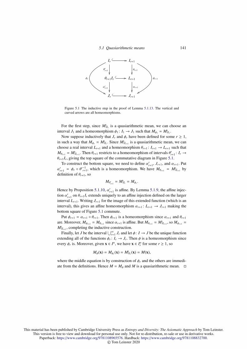
This material has been published by Cambridge University Press as Entropy and Diversity: The Axiomatic Approach by Tom Leinster.This version is free to view and download for personal use only. Not for re-distribution, re-sale or use in derivative works.
Paperback: https://www.cambridge.org/9781108965576. Hardback: https://www.cambridge.org/9781108832700.© Tom Leinster 2020
5.1 Quasiarithmetic means 141
Ir
φr
''
θ′r+1
// Ir+1
φr+1
ww
θr+1
θr+1Ir
//
α′r+1
Lr+1
αr+1
Jr // Jr+1
Figure 5.1 The inductive step in the proof of Lemma 5.1.13. The vertical andcurved arrows are all homeomorphisms.
For the first step, since M|I1 is a quasiarithmetic mean, we can choose aninterval J1 and a homeomorphism φ1 : I1 → J1 such that Mφ1 = M|I1 .
Now suppose inductively that Jr and φr have been defined for some r ≥ 1,in such a way that Mφr = M|Ir . Since M|Ir+1 is a quasiarithmetic mean, we canchoose a real interval Lr+1 and a homeomorphism θr+1 : Ir+1 → Lr+1 such thatMθr+1 = M|Ir+1 . Then θr+1 restricts to a homeomorphism of intervals θ′r+1 : Ir →
θr+1Ir, giving the top square of the commutative diagram in Figure 5.1.To construct the bottom square, we need to define α′r+1, Jr+1, and αr+1. Put
α′r+1 = φr θ′−1r+1, which is a homeomorphism. We have Mθr+1 = M|Ir+1 by
definition of θr+1, so
Mθ′r+1= M|Ir = Mφr .
Hence by Proposition 5.1.10, α′r+1 is affine. By Lemma 5.1.9, the affine injec-tion α′r+1 on θr+1Ir extends uniquely to an affine injection defined on the largerinterval Lr+1. Writing Jr+1 for the image of this extended function (which is aninterval), this gives an affine homeomorphism αr+1 : Lr+1 → Jr+1 making thebottom square of Figure 5.1 commute.
Put φr+1 = αr+1 θr+1. Then φr+1 is a homeomorphism since αr+1 and θr+1
are. Moreover, Mφr+1 = Mθr+1 since αr+1 is affine. But Mθr+1 = M|Ir+1 , so Mφr+1 =
M|Ir+1 , completing the inductive construction.Finally, let J be the interval
⋃∞r=1 Jr and let φ : I → J be the unique function
extending all of the functions φr : Ir → Jr. Then φ is a homeomorphism sinceevery φr is. Moreover, given x ∈ In, we have x ∈ In
r for some r ≥ 1, so
Mφ(x) = Mφr (x) = M|Ir (x) = M(x),
where the middle equation is by construction of φr and the others are immedi-ate from the definitions. Hence M = Mφ and M is a quasiarithmetic mean.

This material has been published by Cambridge University Press as Entropy and Diversity: The Axiomatic Approach by Tom Leinster.This version is free to view and download for personal use only. Not for re-distribution, re-sale or use in derivative works.
Paperback: https://www.cambridge.org/9781108965576. Hardback: https://www.cambridge.org/9781108832700.© Tom Leinster 2020
142 Means
Remark 5.1.14 Kolmogorov found an early characterization theorem forquasiarithmetic means on real intervals [190, 192]. He proved it for closedbounded intervals, and asserted that his argument could be extended to closedunbounded intervals with ‘only a minor modification’ ([192], p. 144). Infact, it can be extended to all intervals. Later authors used results similar toLemma 5.1.13 to prove this and similar statements. For example, the argumentabove is an expansion of the argument on p. 291 of Aczel [2], and of part ofthe proof of Theorem 4.10 of Grabisch, Marichal, Mesiar and Pap [124].
5.2 Unweighted means
In the next three sections, we focus exclusively on means that are unweighted,that is, weighted by the uniform distribution un. Certainly this is a natural spe-cial case. But the real reason for this focus is that the results established willhelp us to prove theorems on weighted means (Section 5.5), which in turn willbe used to prove unique characterizations of measures of value (Section 7.3)and measures of diversity (Section 7.4).
The pattern of argument in this chapter is broadly similar to that in the proofof Faddeev’s theorem (Section 2.5). There, given a hypothetical entropy mea-sure I satisfying some axioms, most of the work went into analysing the se-quence
(I(un)
)n≥1, which then made it relatively easy to find I(p) for distri-
butions p with rational coordinates, and, in turn, for all p. Here, we spendconsiderable time proving results on unweighted means M(un,−). This done,we will quickly be able to deduce results on weighted means M(p,−), first forrational p and then for all p.
For simplicity, we adopt the abbreviated notation
Mt(x) = Mt(un, x)
(t ∈ [−∞,∞], x ∈ [0,∞)n) for unweighted power means, as well as using thenotation Mφ(x) as in equation (5.2).
Let (M : In → I)n≥1 be a sequence of functions, where I is either (0,∞) or[0,∞). Over the next three sections, we answer the question:
What conditions on M guarantee that it is one of the unweighted powermeans Mt?
The question can be interpreted in several ways, depending on whether I is(0,∞) or [0,∞), and also on whether we want to restrict the order t of thepower mean to be positive, finite, etc.
We now list some of the conditions on M that might reasonably be imposed.
This material has been published by Cambridge University Press as Entropy and Diversity: The Axiomatic Approach by Tom Leinster.This version is free to view and download for personal use only. Not for re-distribution, re-sale or use in derivative works.
Paperback: https://www.cambridge.org/9781108965576. Hardback: https://www.cambridge.org/9781108832700.© Tom Leinster 2020
5.2 Unweighted means 143
For many of them, we have already considered similar conditions for weightedmeans (Section 4.2). For Definitions 5.2.1–5.2.13, let I be a real interval andlet (M : In → I)n≥1 be a sequence of functions.
Definition 5.2.1 M is symmetric if M(x) = M(xσ) for all n ≥ 1, x ∈ In, andpermutations σ of 1, . . . , n.
Examples 5.2.2 All quasiarithmetic means are symmetric. So too are all thepower means Mt, including M∞ and M−∞ (which are not quasiarithmetic).
Definition 5.2.3 M is consistent (or idempotent) if
M(x, . . . , x︸ ︷︷ ︸n
) = x
for all n ≥ 1 and x ∈ I.
Example 5.2.4 All quasiarithmetic and power means are consistent.
Definition 5.2.5 M is increasing if for all n ≥ 1 and x, y ∈ In,
x ≤ y =⇒ M(x) ≤ M(y).
It is strictly increasing if for all n ≥ 1 and x, y ∈ In,
x ≤ y , x =⇒ M(x) < M(y).
Example 5.2.6 All quasiarithmetic means are strictly increasing.
Examples 5.2.7 Given a sequence of functions (M : ∆n × In → I)n≥1, ifM is increasing or strictly increasing in the sense of Definition 4.2.18 then(M(un,−) : In → I
)n≥1 is increasing or strictly increasing in the sense above.
In particular, Lemma 4.2.19 implies that:
i. the unweighted power means Mt of all orders t ∈ [−∞,∞] on [0,∞) areincreasing;
ii. the unweighted power means Mt of finite orders t ∈ (−∞,∞) on (0,∞) arestrictly increasing;
iii. the unweighted power means Mt of finite positive orders t ∈ (0,∞) on [0,∞)are strictly increasing.
Examples 5.2.8 i. The power means M∞ = max and M−∞ = min are in-creasing but not strictly so, assuming that the interval I is nontrivial. (Thecounterexample of Remark 4.2.20 is easily adapted to I.) Hence M±∞ arenot quasiarithmetic means.

This material has been published by Cambridge University Press as Entropy and Diversity: The Axiomatic Approach by Tom Leinster.This version is free to view and download for personal use only. Not for re-distribution, re-sale or use in derivative works.
Paperback: https://www.cambridge.org/9781108965576. Hardback: https://www.cambridge.org/9781108832700.© Tom Leinster 2020
144 Means
ii. The power means Mt of order t ∈ [−∞, 0] are not strictly increasing on[0,∞) (again, as in Remark 4.2.20). So they are not quasiarithmetic on[0,∞), even though they are quasiarithmetic on (0,∞).
Definition 5.2.9 M is decomposable if for all n, k1, . . . , kn ≥ 1 and xij ∈ I,
M(x1
1, . . . , x1k1, . . . , xn
1, . . . , xnkn
)= M(a1, . . . , a1︸ ︷︷ ︸
k1
, . . . , an, . . . , an︸ ︷︷ ︸kn
),
where ai = M(xi
1, . . . , xiki
)for i ∈ 1, . . . , n.
We adopt the shorthand
r ∗ x = x, . . . , x︸ ︷︷ ︸r
(5.3)
whenever r ≥ 1 and x ∈ R. Thus, the decomposability equation becomes
M(x1
1, . . . , x1k1, . . . , xn
1, . . . , xnkn
)= M(k1 ∗ a1, . . . , kn ∗ an).
Decomposability is an unweighted analogue of the chain rule for weightedmeans (Definition 4.2.23), as the following examples show.
Examples 5.2.10 i. For each t ∈ [−∞,∞], the power mean Mt is decom-posable. This can of course be shown by direct calculation, but instead weprove it using earlier results on weighted power means.
Take xij and ai as in Definition 5.2.9. Write
k = k1 + · · · + kn, p = (k1/k, . . . , kn/k) ∈ ∆n.
Then
p (uk1 , . . . ,ukn ) = uk,
so
Mt(x11, . . . , x
1k1, . . . , xn
1, . . . , xnkn
)
= Mt(p (uk1 , . . . ,ukn ),
(x1
1, . . . , x1k1
)⊕ · · · ⊕
(xn
1, . . . , xnkn
))= Mt
(p, (a1, . . . , an)
),
by the chain rule for power means (Proposition 4.2.24). On the other hand,
Mt(k1 ∗ a1, . . . , kn ∗ an)
= Mt(p (uk1 , . . . ,ukn ), (k1 ∗ a1) ⊕ · · · ⊕ (kn ∗ an)
)= Mt
(p,
(Mt(uk1 , k1 ∗ a1), . . . ,Mt(ukn , kn ∗ an)
))= Mt
(p, (a1, . . . , an)
),
by the chain rule again and consistency of Mt. Hence Mt is decomposable.

This material has been published by Cambridge University Press as Entropy and Diversity: The Axiomatic Approach by Tom Leinster.This version is free to view and download for personal use only. Not for re-distribution, re-sale or use in derivative works.
Paperback: https://www.cambridge.org/9781108965576. Hardback: https://www.cambridge.org/9781108832700.© Tom Leinster 2020
5.2 Unweighted means 145
ii. In particular, M1 is decomposable, from which it follows that all quasi-arithmetic means are decomposable.
Remark 5.2.11 In the literature, decomposability is often stated in the asym-metric form
M(x1, . . . , xk, y1, . . . , y`) = M(k ∗ a, y1, . . . , y`)
(k, ` ≥ 1, xi, y j ∈ I), where a = M(x1, . . . , xk). (This was the form used byboth Kolmogorov [190, 192] and Nagumo [257], for instance.) Under the mildassumptions that M is symmetric and consistent, this is equivalent to the defi-nition above, by a straightforward induction.
Definition 5.2.12 M is modular if for all
x11, . . . , x
1k1, . . . , xn
1, . . . , xnkn∈ I, y1
1, . . . , y1k1, . . . , yn
1, . . . , ynkn∈ I
such that
M(xi
1, . . . , xiki
)= M
(yi
1, . . . , yiki
)for each i, we have
M(x1
1, . . . , x1k1, . . . , xn
1, . . . , xnkn
)= M
(y1
1, . . . , y1k1, . . . , yn
1, . . . , ynkn
).
In other words, M is modular if
M(x1
1, . . . , x1k1, . . . , xn
1, . . . , xnkn
)is determined by k1, . . . , kn and
M(x1
1, . . . , xn1), . . . , M
(xn
1, . . . , xnkn
).
Evidently this is true if M is decomposable.
Definition 5.2.13 Suppose that I is closed under multiplication. Then M ishomogeneous if
M(cx) = cM(x)
for all n ≥ 1, c ∈ I, and x ∈ In.
Examples 5.2.14 All the power means are homogeneous. But other quasi-arithmetic means are not, as Theorem 5.1.12 shows.
It has already been mentioned that an important early result in the the-ory of means was proved by Kolmogorov and Nagumo, independently in1930 [190, 257]. What they showed was that any continuous, symmetric, con-sistent, strictly increasing, decomposable sequence of functions (M : In →
I)n≥1 on a real interval I is a quasiarithmetic mean.

This material has been published by Cambridge University Press as Entropy and Diversity: The Axiomatic Approach by Tom Leinster.This version is free to view and download for personal use only. Not for re-distribution, re-sale or use in derivative works.
Paperback: https://www.cambridge.org/9781108965576. Hardback: https://www.cambridge.org/9781108832700.© Tom Leinster 2020
146 Means
One of the purposes of this book is to prove characterization theorems fordiversity measures. The measures that we characterize are closely related tothe power means Mt, where t ∈ [−∞,∞]. In particular, we want to includeM±∞. Since Kolmogorov and Nagumo’s theorem insists on a strictly increasingmean, it is inadequate for our purpose. So, we follow a different path.
There is another difference between the results below and those of Kol-mogorov and Nagumo. Our focus on power means makes it natural to impose ahomogeneity condition (in the light of Theorem 5.1.12). It turns out that whenhomogeneity is assumed, the continuity condition in the Kolmogorov–Nagumotheorem can be dropped.
In Section 5.3, we will characterize the power means of finite orders t ∈(−∞,∞). We will use this result in Section 5.4 to achieve our goal of charac-terizing the power means of all orders t ∈ [−∞,∞]. Our first steps are the sameas the first steps of Kolmogorov’s proof, and most of the lemmas in the re-mainder of this section can be found in his paper [190] (translated into Englishas [192]).
Our first lemma concerns repetition of terms.
Lemma 5.2.15 Let I be an interval and let (M : In → I)n≥1 be a symmetric,consistent, decomposable sequence of functions. Then
M(r ∗ x1, . . . , r ∗ xn) = M(x1, . . . , xn) (5.4)
for all r, n ≥ 1 and x1, . . . , xn ∈ I.
Proof Write a = M(x1, . . . , xn). By symmetry, the left-hand side of equa-tion (5.4) is equal to
M(x1, . . . , xn, . . . , x1, . . . , xn),
with rn terms in total. By decomposability, this is equal to M(rn ∗ a), which byconsistency is equal to a.
The next group of lemmas begins to answer the question: given a quasi-arithmetic mean M on an interval I, how can we construct from M a home-omorphism φ such that M = Mφ? Proposition 5.1.10 tells us that there aremany homeomorphisms with this property. But it also tells us that if I is ofthe form [a, b] for some real a < b, then there is a unique homeomorphismφ : [a, b] → [0, 1] such that φ(a) = 0, φ(b) = 1, and M = Mφ. The function ψconstructed in the next lemma will turn out to be the inverse of φ, restricted tothe rationals.
Lemma 5.2.16 Let a, b ∈ R with a < b. Let(M : [a, b]n → [a, b]
)n≥1 be a
symmetric, consistent, decomposable sequence of functions.

This material has been published by Cambridge University Press as Entropy and Diversity: The Axiomatic Approach by Tom Leinster.This version is free to view and download for personal use only. Not for re-distribution, re-sale or use in derivative works.
Paperback: https://www.cambridge.org/9781108965576. Hardback: https://www.cambridge.org/9781108832700.© Tom Leinster 2020
5.2 Unweighted means 147
i. There is a unique function
ψ : [0, 1] ∩ Q→ [a, b]
satisfying
ψ(r/s) = M((s − r) ∗ a, r ∗ b
)for all integers 0 ≤ r ≤ s with s ≥ 1.
ii. ψ(0) = a and ψ(1) = b.
iii. For all n ≥ 1 and q1, . . . , qn ∈ [0, 1] ∩ Q,
M(ψ(q1), . . . , ψ(qn)
)= ψ
(1n
n∑i=1
qi
).
iv. If M is increasing then so is ψ, and if M is strictly increasing then so is ψ.
Proof For (i), uniqueness is immediate. To prove existence, we must show thatdifferent representations r/s of the same rational number give the same valueof M((s − r) ∗ a, r ∗ b). Suppose that r/s = r′/s′. Then s′r = sr′, so usingLemma 5.2.15 twice,
M((s − r) ∗ a, r ∗ b
)= M
(s′(s − r) ∗ a, s′r ∗ b
)= M
(s(s′ − r′) ∗ a, sr′ ∗ b
)= M
((s′ − r′) ∗ a, r′ ∗ b
).
This proves (i), and (ii) follows from the formula for ψ and consistency.For (iii), express q1, . . . , qn as fractions over a common denominator, say
qi = ri/s. Then
M(ψ(q1), . . . , ψ(qn)
)= M
(s ∗ ψ(q1), . . . , s ∗ ψ(qn)
)(5.5)
= M((s − r1) ∗ a, r1 ∗ b, . . . , (s − rn) ∗ a, rn ∗ b
)(5.6)
= M((ns − r1 − · · · − rn) ∗ a, (r1 + · · · + rn) ∗ b
)(5.7)
= ψ( r1 + · · · + rn
ns
)= ψ
(1n
n∑i=1
qi
),
where equation (5.5) uses Lemma 5.2.15, equation (5.6) follows from decom-posability and the definition of ψ, and equation (5.7) is by symmetry.
For (iv), let q, q′ ∈ [0, 1]∩Qwith q < q′. We may write q = r/s and q′ = r′/s

This material has been published by Cambridge University Press as Entropy and Diversity: The Axiomatic Approach by Tom Leinster.This version is free to view and download for personal use only. Not for re-distribution, re-sale or use in derivative works.
Paperback: https://www.cambridge.org/9781108965576. Hardback: https://www.cambridge.org/9781108832700.© Tom Leinster 2020
148 Means
for some integers 0 ≤ r < r′ ≤ s with s ≥ 1. Assuming that M is increasing,
M(q) = M((s − r) ∗ a, r ∗ b
)= M
((s − r′) ∗ a, (r′ − r) ∗ a, r ∗ b
)≤ M
((s − r′) ∗ a, (r′ − r) ∗ b, r ∗ b
)(5.8)
= M((s − r′) ∗ a, r′ ∗ b
)= M(q′),
with strict inequality in (5.8) if M is strictly increasing.
We will chiefly be working with decomposable, homogeneous means on(0,∞). Such a mean is automatically consistent:
Lemma 5.2.17 Let(M : (0,∞)n → (0,∞)
)n≥1 be a decomposable, homoge-
neous sequence of functions. Then M is consistent.
Proof For k ≥ 1, write ak = M(k∗1). By decomposability, ak = M(k∗ak). (Thisfollows from Definition 5.2.9 by taking n = 1, k1 = k, and x1
1 = · · · = x1k = 1.)
Hence by homogeneity, ak = ak M(k ∗ 1) = a2k , giving ak ∈ 0, 1. But M takes
values in (0,∞), so ak = 1. Thus, for all x ∈ (0,∞)k,
M(k ∗ x) = xak = x
by homogeneity again.
We will deduce that any symmetric such mean is multiplicative, in the fol-lowing sense.
Definition 5.2.18 Let I be a real interval closed under multiplication. A se-quence of functions (M : In → I)n≥1 is multiplicative if
M(x ⊗ y) = M(x)M(y)
for all n,m ≥ 1, x ∈ In, and y ∈ Im.
For instance, if a weighted mean is multiplicative in the sense of Defini-tion 4.2.27 then its unweighted part
(M(un,−)
)n≥1 is multiplicative in the sense
just defined.
Lemma 5.2.19 Let(M : (0,∞)n → (0,∞)
)n≥1 be a symmetric, decomposable,
homogeneous sequence of functions. Then M is multiplicative.
Proof By Lemma 5.2.17, M is consistent. Let x ∈ (0,∞)n and y ∈ (0,∞)m.Writing
bi = M(xiy1, . . . , xiym),
This material has been published by Cambridge University Press as Entropy and Diversity: The Axiomatic Approach by Tom Leinster.This version is free to view and download for personal use only. Not for re-distribution, re-sale or use in derivative works.
Paperback: https://www.cambridge.org/9781108965576. Hardback: https://www.cambridge.org/9781108832700.© Tom Leinster 2020
5.3 Strictly increasing homogeneous means 149
we have
M(x ⊗ y) = M(m ∗ b1, . . . ,m ∗ bn) = M(b1, . . . , bn), (5.9)
by decomposability and Lemma 5.2.15 respectively. But by homogeneity,bi = xiM(y). Substituting this into (5.9) and using homogeneity again givesthe result.
Lemmas 5.2.15–5.2.19 are largely taken from Kolmogorov [190, 192], who,assuming that M is continuous, went on to prove that the function ψ ofLemma 5.2.16 extends to a continuous function on [0, 1]. But this is wherehis path and ours diverge.
5.3 Strictly increasing homogeneous means
Here we prove two theorems on strictly increasing, symmetric, decomposable,homogeneous, unweighted means (Table 5.1). First we show that on (0,∞),such means are exactly the power means of finite order. From this we deducethat on [0,∞), the means with these properties are exactly the power means offinite positive order.
To show that any sequence of functions(M : (0,∞)n → (0,∞)
)n≥1 with suit-
able properties is a power mean of finite order, the main challenge is to showthat M is quasiarithmetic. We do this by showing that the restriction of M toeach closed bounded subinterval K ⊂ (0,∞) is quasiarithmetic, then invokingLemma 5.1.13. An important part of the proof that M|K is quasiarithmetic willbe to take the map
ψ : [0, 1] ∩ Q→ K
provided by Lemma 5.2.16 and extend it to a map [0, 1]→ K. For this, we usea lemma of real analysis that has nothing intrinsically to do with means.
Lemma 5.3.1 Let ψ : [0, 1]∩Q→ R be a strictly increasing function. Supposethat for all z ∈ [0, 1),
supψ(p) : rational p ≤ z = infψ(q) : rational q > z, (5.10)
and for all z ∈ (0, 1],
supψ(p) : rational p < z = infψ(q) : rational q ≥ z. (5.11)
Then ψ extends uniquely to a continuous function [0, 1]→ R, and this extendedfunction is strictly increasing.

This material has been published by Cambridge University Press as Entropy and Diversity: The Axiomatic Approach by Tom Leinster.This version is free to view and download for personal use only. Not for re-distribution, re-sale or use in derivative works.
Paperback: https://www.cambridge.org/9781108965576. Hardback: https://www.cambridge.org/9781108832700.© Tom Leinster 2020
150 Means
Equations (5.10) and (5.11) can be understood as follows. Taken over ratio-nal z, they together state that the function ψ : [0, 1] ∩ Q → R is continuous.When z is irrational, both (5.10) and (5.11) reduce to the equation
supψ(p) : rational p < z = infψ(q) : rational q > z,
which states that ψ has no jump discontinuity at z. Thus, the result is that anycontinuous, strictly increasing function on [0, 1] ∩ Q extends to a function on[0, 1] with the same properties, as long as the original function has no jumpdiscontinuities.
Proof Uniqueness is immediate. For existence, first note that
supψ(p) : rational p ≤ z = infψ(q) : rational q ≥ z (5.12)
for all z ∈ [0, 1]. Indeed, if z ∈ Q then both sides are equal to ψ(z) (since ψis increasing), and if z < Q then (5.12) is equivalent to both (5.10) and (5.11).Define a function ψ : [0, 1]→ R by taking ψ(z) to be either side of (5.12). Thenψ|Q = ψ.
To see that ψ is strictly increasing, let z, z′ ∈ [0, 1] with z < z′. We canchoose rational q and p such that z ≤ q < p ≤ z′. Then by definition of ψ andthe fact that ψ is strictly increasing,
ψ(z) ≤ ψ(q) < ψ(p) ≤ ψ(z′),
as required.Finally, we show that ψ is continuous. Since ψ is increasing, it suffices to
show that for all z ∈ [0, 1),
ψ(z) = infψ(w) : w > z
,
and for all z ∈ (0, 1],
ψ(z) = supψ(w) : w < z
.
We prove just the first of these equations, the second being similar. Let z ∈[0, 1). Then
infψ(w) : w > z
= inf
infψ(q) : rational q ≥ w : w > z
(5.13)
= inf⋃w>z
ψ(q) : rational q ≥ w
= infψ(q) : rational q > z
= infψ(q) : rational q ≥ z (5.14)
= ψ(z), (5.15)

This material has been published by Cambridge University Press as Entropy and Diversity: The Axiomatic Approach by Tom Leinster.This version is free to view and download for personal use only. Not for re-distribution, re-sale or use in derivative works.
Paperback: https://www.cambridge.org/9781108965576. Hardback: https://www.cambridge.org/9781108832700.© Tom Leinster 2020
5.3 Strictly increasing homogeneous means 151
(0,∞)n M // (0,∞)
Kn?
OO
M|K //
φn
K?
OO
φ
[0, 1]n
ψn
ZZ
M1
// [0, 1]
ψ
ZZ
[0, 1] ∩ Q? _oo
ψnn
Figure 5.2 Maps involved in the proof of Theorem 5.3.2.
where (5.13) and (5.15) are by definition of ψ, and (5.14) follows from (5.10)and (5.12).
We now prove our characterization theorem for strictly increasing un-weighted means on (0,∞) (Figure 5.2).
Theorem 5.3.2 Let(M : (0,∞)n → (0,∞)
)n≥1 be a sequence of functions. The
following are equivalent:
i. M is symmetric, strictly increasing, decomposable, and homogeneous;ii. M = Mt for some t ∈ (−∞,∞).
Proof (ii) implies (i) by Examples 5.2.2, 5.2.7(ii), 5.2.10(i), and 5.2.14.Now assume (i). The main part of the proof is to show that M restricts to
a quasiarithmetic mean on each nontrivial closed bounded subinterval K ⊂(0,∞). Let K be such an interval.
First note that for each n ≥ 1, the function M : (0,∞)n → (0,∞) restrictsto a function M|K : Kn → K. Indeed, M is consistent by Lemma 5.2.17, andincreasing, so for all x1, . . . , xn ∈ K,
minx1, . . . , xn ≤ M(x1, . . . , xn) ≤ maxx1, . . . , xn,
giving M(x1, . . . , xn) ∈ K.Next we show that the sequence of functions (M|K : Kn → K)n≥1 is a quasi-
arithmetic mean. This sequence is symmetric, consistent, strictly increasingand decomposable, since M is. Let ψ : [0, 1] ∩ Q → K be the function definedin Lemma 5.2.16. We will extend ψ to a continuous function [0, 1]→ K usingLemma 5.3.1. For this, we have to verify the hypotheses of that lemma: that ψis strictly increasing (which is immediate from Lemma 5.2.16(iv)) and that ψsatisfies equations (5.10) and (5.11). We prove only (5.10), the proof of (5.11)being similar.
This material has been published by Cambridge University Press as Entropy and Diversity: The Axiomatic Approach by Tom Leinster.This version is free to view and download for personal use only. Not for re-distribution, re-sale or use in derivative works.
Paperback: https://www.cambridge.org/9781108965576. Hardback: https://www.cambridge.org/9781108832700.© Tom Leinster 2020
152 Means
Let z ∈ [0, 1). Put
u = supψ(p) : rational p ≤ z, v = infψ(q) : rational q > z.
We have to show that u = v. Since ψ is increasing, u ≤ v. It remains to showthat u ≥ v.
Let C > 1. We have v ∈ K ⊂ (0,∞), so v > 0, giving Cv > v. By definitionof v, we can therefore choose a rational q ∈ (z, 1] such that ψ(q) ≤ Cv. We canthen choose a rational p ∈ [0, z] such that 1
2 (p + q) > z. By definition of u, wehave ψ(p) ≤ u ≤ Cu. Now
CM(u, v) = M(Cu,Cv) (5.16)
≥ M(ψ(p), ψ(q)) (5.17)
= ψ( 1
2 (p + q))
(5.18)
≥ v, (5.19)
where (5.16) is by homogeneity, (5.17) is because M is increasing, (5.18) fol-lows from Lemma 5.2.16(iii), and (5.19) is because 1
2 (p+q) ∈ (z, 1]∩Q. HenceCM(u, v) ≥ v for all C > 1, giving M(u, v) ≥ v. But then
v = M(v, v) ≥ M(u, v) ≥ v
(using consistency), so M(v, v) = M(u, v). Since M is strictly increasing, thisforces u = v, proving equation (5.10) in Lemma 5.3.1.
We have now shown that the function ψ : [0, 1] ∩ Q → K satisfies the hy-potheses of Lemma 5.3.1. By that lemma, ψ extends uniquely to a continuous,strictly increasing function [0, 1] → K, which we also denote by ψ. The ex-tended function ψ is endpoint-preserving by Lemma 5.2.16(ii), and is thereforea homeomorphism. Let φ : K → [0, 1] be its inverse.
We will prove that M|K = Mφ, or equivalently that
M(ψ(z1), . . . , ψ(zn)
)= ψ
( 1n (z1 + · · · + zn)
)(5.20)
(zi ∈ [0, 1]). Indeed, for all z1, . . . , zn ∈ [0, 1],
M(ψ(z1), . . . , ψ(zn)
)≥ sup
M
(ψ(q1), . . . , ψ(qn)
): rational qi ≤ zi
(5.21)
= supψ( 1
n (q1 + · · · + qn))
: rational qi ≤ zi
(5.22)
= ψ(sup
1n (q1 + · · · + qn) : rational qi ≤ zi
)(5.23)
= ψ( 1
n (z1 + · · · + zn)), (5.24)
where (5.21) holds because M and ψ are increasing, (5.22) follows from

This material has been published by Cambridge University Press as Entropy and Diversity: The Axiomatic Approach by Tom Leinster.This version is free to view and download for personal use only. Not for re-distribution, re-sale or use in derivative works.
Paperback: https://www.cambridge.org/9781108965576. Hardback: https://www.cambridge.org/9781108832700.© Tom Leinster 2020
5.3 Strictly increasing homogeneous means 153
Lemma 5.2.16(iii), equation (5.23) is a consequence of ψ : [0, 1] → K being astrictly increasing bijection, and (5.24) is elementary. So
M(ψ(z1), . . . , ψ(zn)
)≥ ψ
( 1n (z1 + · · · + zn)
).
The same argument with the inequalities reversed and the suprema changed toinfima proves the opposite inequality, and equation (5.20) follows. So M|K =
Mφ, as claimed.We have now shown that M restricts to a quasiarithmetic mean on each
nontrivial closed bounded subinterval of (0,∞). Hence by Lemma 5.1.13, Mitself is a quasiarithmetic mean. But M is homogeneous, so Theorem 5.1.12now implies that M = Mt for some t ∈ (−∞,∞).
From this theorem about means on (0,∞), we deduce a theorem about meanson [0,∞).
Theorem 5.3.3 Let(M : [0,∞)n → [0,∞)
)n≥1 be a sequence of functions. The
following are equivalent:
i. M is symmetric, strictly increasing, decomposable, and homogeneous;ii. M = Mt for some t ∈ (0,∞).
Proof Certainly (ii) implies (i), by Examples 5.2.2–5.2.14. Now assume (i). If0 , x ∈ [0,∞)n then M(x) > M(0) ≥ 0, so M(x) > 0. Hence M restricts to asequence of functions
M|(0,∞) : (0,∞)n → (0,∞).
By Theorem 5.3.2, M|(0,∞) = Mt for some t ∈ (−∞,∞).To show that t > 0, note that
0 < M(1, 0) ≤ infδ>0
M(1, δ) = infδ>0
Mt(1, δ) = Mt(1, 0),
where in the last step we used the fact that Mt is continuous (Lemma 4.2.5)and increasing. Hence Mt(1, 0) > 0. But Mt(1, 0) = 0 for all t ∈ [−∞, 0](Definition 4.2.1), so t ∈ (0,∞).
We now have to show that the equality M(x) = Mt(x), so far proved to holdfor all x ∈ (0,∞)n, holds for all x ∈ [0,∞)n.
First I claim that
M(1, 0) = Mt(1, 0). (5.25)
To prove this, we evaluate M(2, 1, 0) in two ways. Put a = M(1, 0) > 0. Since

This material has been published by Cambridge University Press as Entropy and Diversity: The Axiomatic Approach by Tom Leinster.This version is free to view and download for personal use only. Not for re-distribution, re-sale or use in derivative works.
Paperback: https://www.cambridge.org/9781108965576. Hardback: https://www.cambridge.org/9781108832700.© Tom Leinster 2020
154 Means
M is decomposable,
M(2, 1, 0) = M(2, a, a)
= Mt(2, a, a)
=(
13 (2t + 2at)
)1/t.
On the other hand, M(2, 0) = 2a by homogeneity, so, using decomposabilityagain,
M(2, 1, 0) = M(1, 2, 0)
= M(1, 2a, 2a)
= Mt(1, 2a, 2a)
=( 1
3 (1 + 2t+1at))1/t
.
Equating these two expressions for M(2, 1, 0) gives a = (1/2)1/t, or equiva-lently, M(1, 0) = Mt(1, 0), as claimed.
Now we prove that M(x) = Mt(x) for all n ≥ 1 and x ∈ [0,∞)n. By symme-try, it suffices to prove this when
x = (x1, . . . , xm, k ∗ 0)
for some k,m ≥ 0 and x1, . . . , xm > 0. The proof is by induction on k for allm simultaneously. We already have the result for k = 0. Suppose now thatk ≥ 1 and the result holds for k − 1. If m = 0 then the result is trivial (byhomogeneity), so suppose that m ≥ 1. We have
M(x1, . . . , xm, k ∗ 0)
= M(x1, . . . , xm−1, xm, 0, (k − 1) ∗ 0
)= M
(x1, . . . , xm−1, xmM(1, 0), xmM(1, 0), (k − 1) ∗ 0
)(5.26)
= M(x1, . . . , xm−1, xmMt(1, 0), xmMt(1, 0), (k − 1) ∗ 0
)(5.27)
= Mt(x1, . . . , xm−1, xmMt(1, 0), xmMt(1, 0), (k − 1) ∗ 0
)(5.28)
= Mt(x1, . . . , xm−1, xm, 0, (k − 1) ∗ 0
)(5.29)
= Mt(x1, . . . , xm, k ∗ 0),
where equations (5.26) and (5.29) are by decomposability and homogeneity ofM and Mt, equation (5.27) follows from equation (5.25), and equation (5.28)is by inductive hypothesis. This completes the proof.

This material has been published by Cambridge University Press as Entropy and Diversity: The Axiomatic Approach by Tom Leinster.This version is free to view and download for personal use only. Not for re-distribution, re-sale or use in derivative works.
Paperback: https://www.cambridge.org/9781108965576. Hardback: https://www.cambridge.org/9781108832700.© Tom Leinster 2020
5.4 Increasing homogeneous means 155
5.4 Increasing homogeneous means
The extremal cases M±∞ of the power means are neither strictly increasingnor quasiarithmetic. Both of these factors put M±∞ outside the ambit of manycharacterizations of means. However, we will prove characterization theoremsthat include M±∞, mostly so as not to exclude the important Berger–Parker in-dex D∞ (Example 4.3.5(iv)) from a later characterization theorem for diversitymeasures.
We have already characterized the strictly increasing means, so our task nowis to characterize the means M that are increasing but not strictly so. Assumingsymmetry, we have
M(x1, . . . , xm, u) = M(x1, . . . , xm, v)
for some xi, u, v with u , v. Our aim is to deduce from this equation, andthe usual other hypotheses on M, that M is equal to either M∞ = max orM−∞ = min.
Lemma 5.4.1 Let I be a real interval. Let (M : In → I)n≥1 be a symmetric,decomposable sequence of functions. Let m ≥ 1 and x1, . . . , xm, u, v ∈ I with
M(x1, . . . , xm, u) = M(x1, . . . , xm, v).
Then
M(x1, . . . , xm, n ∗ u) = M(x1, . . . , xm, n ∗ v)
for all n ≥ 0.
Proof This is trivial for n = 0. Suppose inductively that n ≥ 0 and the resultholds for n. Since M is decomposable, it is modular (Definition 5.2.12). Now
M(x1, . . . , xm, (n + 1) ∗ u
)= M(x1, . . . , xm, n ∗ u, u)
= M(x1, . . . , xm, n ∗ v, u) (5.30)
= M(x1, . . . , xm, u, n ∗ v) (5.31)
= M(x1, . . . , xm, v, n ∗ v) (5.32)
= M(x1, . . . , xm, (n + 1) ∗ v
),
where (5.30) and (5.32) use modularity and (5.31) is by symmetry.
We deduce:
Lemma 5.4.2 Let I be an interval and let (M : In → I)n≥1 be a sequence offunctions that is symmetric, consistent, decomposable, and increasing but notstrictly so. Then there exist x, u, v ∈ I such that u , v but M(x, u) = M(x, v).

This material has been published by Cambridge University Press as Entropy and Diversity: The Axiomatic Approach by Tom Leinster.This version is free to view and download for personal use only. Not for re-distribution, re-sale or use in derivative works.
Paperback: https://www.cambridge.org/9781108965576. Hardback: https://www.cambridge.org/9781108832700.© Tom Leinster 2020
156 Means
Proof By symmetry, there exist n ≥ 0 and x1, . . . , xn, u, v ∈ I such that u , vand
M(x1, . . . , xn, u) = M(x1, . . . , xn, v).
By consistency, n ≥ 1. Writing x = M(x1, . . . , xn), we have
M(n ∗ x, u) = M(n ∗ x, v)
by decomposability. Now
M(x, u) = M(n ∗ x, n ∗ u) = M(n ∗ x, n ∗ v) = M(x, v),
where the first and last equalities follow from Lemma 5.2.15 and the secondfrom Lemma 5.4.1.
Our next lemma contains the main substance of the argument that if M isincreasing but not strictly so, then M = M±∞.
Lemma 5.4.3 Let(M : (0,∞)n → (0,∞)
)n≥1 be a symmetric, increasing, de-
composable, homogeneous sequence of functions. If there exist x ∈ (0,∞) anddistinct u, v ≥ x such that M(x, u) = M(x, v), then there exist a < b in (0,∞)such that M(a, b) = a.
Proof Take x, u and v as described. We may assume without loss of generalitythat u < v and (by homogeneity) that x = 1. We may therefore choose a realnumber C > 1 and an integer N ≥ 1 such that u ≤ CN < CN+1 ≤ v. We willprove that M(1,CN) = 1.
Since M is increasing, the hypothesis that M(1, u) = M(1, v) implies that
M(1,CN)
= M(1,CN+1).
It follows from Lemma 5.4.1 that
M(1, r ∗CN)
= M(1, r ∗CN+1)
for all r ≥ 0, then by homogeneity that
M(C s, r ∗C s+N)
= M(C s, r ∗C s+N+1) (5.33)
for all r, s ≥ 0.I claim that
M(1, r ∗Ck) ≤ CN (5.34)
for all k, r ≥ 0. To prove this, first note that M is consistent, by Lemma 5.2.17.When k ≤ N, we have Ck ≤ CN , so (5.34) holds because M is consistent and

This material has been published by Cambridge University Press as Entropy and Diversity: The Axiomatic Approach by Tom Leinster.This version is free to view and download for personal use only. Not for re-distribution, re-sale or use in derivative works.
Paperback: https://www.cambridge.org/9781108965576. Hardback: https://www.cambridge.org/9781108832700.© Tom Leinster 2020
5.4 Increasing homogeneous means 157
increasing. Now let k ≥ N and suppose inductively that (5.34) holds for k, forall r. Then for all r,
M(1, r ∗Ck+1) = M
(1, 1, 2r ∗Ck+1) (5.35)
≤ M(1,Ck−N , 2r ∗Ck+1) (5.36)
= M(1,Ck−N , 2r ∗Ck) (5.37)
≤ M(1, (2r + 1) ∗Ck) (5.38)
≤ CN , (5.39)
where equation (5.35) follows from Lemma 5.2.15, inequality (5.36) from thefact that Ck−N ≥ 1, equation (5.37) from (5.33) (with s = k − N) and decom-posability, inequality (5.38) from the fact that Ck−N ≤ Ck, and inequality (5.39)from the inductive hypothesis. This completes the induction and the proof ofthe claimed inequality (5.34).
It follows from (5.34) that
M(1,Ck1 , . . . ,Ckr
)≤ CN (5.40)
for all r, k1, . . . , kr ≥ 0. Indeed, since M is increasing, the left-hand sideof (5.40) is at most M
(1, r ∗Cmax ki
), which by (5.34) is at most CN .
We finish by using the tensor power trick (Tao [322], Section 1.9). For allr ≥ 1,
M(1,CN)
= M((
1,CN)⊗r)1/r
by Lemma 5.2.19. Expanding the tensor power(1,CN)⊗r
=(1,CN)
⊗ · · · ⊗(1,CN)
gives
M(1,CN)
= M(1,
(r1
)∗CN , . . . ,
(r
r − 1
)∗C(r−1)N ,CrN
)1/r
≤ CN/r
for all r ≥ 1, by symmetry of M and inequality (5.40). Letting r → ∞, thisproves that M(1,CN) ≤ 1. But also
M(1,CN)
≥ M(1, 1) = 1,
since M is increasing and consistent. Hence M(1,CN) = 1 with CN > 1, com-pleting the proof.
The lemma just proved states that under certain hypotheses, M(a, b) =
mina, b for some distinct numbers a and b. The next lemma tells us that in that

This material has been published by Cambridge University Press as Entropy and Diversity: The Axiomatic Approach by Tom Leinster.This version is free to view and download for personal use only. Not for re-distribution, re-sale or use in derivative works.
Paperback: https://www.cambridge.org/9781108965576. Hardback: https://www.cambridge.org/9781108832700.© Tom Leinster 2020
158 Means
case, M(a, b) = mina, b for all a and b. Better still, M(x1, . . . , xn) = min xi
for all n ≥ 1 and all xi.
Lemma 5.4.4 Let(M : (0,∞)n → (0,∞)
)n≥1 be a symmetric, increasing, de-
composable, homogeneous sequence of functions. If M(a, b) = a for some0 < a < b then M = M−∞.
Proof By homogeneity, we may assume that a = 1, so that b > 1 withM(1, b) = 1.
First I claim that M(1, br) = 1 for all r ≥ 0. By Lemma 5.2.17, M is con-sistent, which gives the case r = 0. Now suppose inductively that r ≥ 1 withM(1, br−1) = 1. By Lemma 5.2.15 and the fact that M is increasing,
M(1, br) = M(1, 1, br, br) ≤ M(1, b, br, br). (5.41)
By inductive hypothesis and homogeneity, M(b, br) = b. Hence, using decom-posability twice,
M(1, b, br, br) = M(1, b, b, br) = M(1, b, b, b). (5.42)
But M(1, b) = 1 = M(1, 1) by hypothesis and consistency, so by Lemma 5.4.1,
M(1, b, b, b) = M(1, 1, 1, 1) = 1. (5.43)
Putting together (5.41), (5.42) and (5.43) gives M(1, br) ≤ 1. But alsoM(1, br) ≥ M(1, 1) = 1, so M(1, br) = 1, completing the induction and provingthe claim.
Next I claim that
M(x, y) = minx, y (5.44)
for all x, y ∈ (0,∞). By homogeneity, it is enough to prove this when x = 1 ≤ y;then our task is to prove that M(1, y) = 1 for all y ≥ 1. Certainly
M(1, y) ≥ M(1, 1) = 1.
On the other hand, we can choose r ≥ 0 such that y ≤ br, and then
M(1, y) ≤ M(1, br) = 1
by the claim above. Hence M(1, y) = 1, as claimed.Finally, we prove that
M(x1, . . . , xn) = minx1, . . . , xn
for all n ≥ 1 and x ∈ (0,∞)n. By symmetry, we may assume that x1 = mini xi.

This material has been published by Cambridge University Press as Entropy and Diversity: The Axiomatic Approach by Tom Leinster.This version is free to view and download for personal use only. Not for re-distribution, re-sale or use in derivative works.
Paperback: https://www.cambridge.org/9781108965576. Hardback: https://www.cambridge.org/9781108832700.© Tom Leinster 2020
5.4 Increasing homogeneous means 159
(0,∞)n M //
ρn
(0,∞)
ρ
(0,∞)n
M// (0,∞)
Figure 5.3 Commutative diagram showing the relationship between a mean Mand its dual M, where ρ : x 7→ 1/x is the reciprocal map.
Then M(x1, xi) = x1 for all i, by equation (5.44). Hence
M(x1, x2, x3, x4, . . . , xn) = M(x1, x1, x3, x4, . . . , xn)
= M(x1, x1, x1, x4, . . . , xn)
= . . .
= M(x1, x1, x1, x1, . . . , x1)
= x1,
where the first equality follows from decomposability and the fact thatM(x1, x2) = x1, the second from decomposability and the fact that M(x1, x3) =
x1, and so on, while the last equality follows from the consistency of M.
So far, we have focused on M−∞ = min rather than M∞ = max. Of course,similar results hold for M∞ by reversing all the inequalities, but the situation ishandled most systematically by the following duality construction (Figure 5.3).Given a sequence of functions
(M : (0,∞)n → (0,∞)
)n≥1, define another such
sequence M by
M(x1, . . . , xn) =1
M( 1
x1, . . . , 1
xn
)(x1, . . . , xn ∈ (0,∞)). For example, equation (4.11) (p. 105) implies that
Mt = M−t
for all t ∈ [−∞,∞]. Evidently M = M for any M.We will use without mention the following lemma, whose proof is trivial:
Lemma 5.4.5 Let (M : (0,∞)n → (0,∞))n≥1 be a sequence of functions. ThenM is symmetric, consistent, increasing, strictly increasing, decomposable orhomogeneous (respectively) if and only if M is.
The next result uses this duality.

This material has been published by Cambridge University Press as Entropy and Diversity: The Axiomatic Approach by Tom Leinster.This version is free to view and download for personal use only. Not for re-distribution, re-sale or use in derivative works.
Paperback: https://www.cambridge.org/9781108965576. Hardback: https://www.cambridge.org/9781108832700.© Tom Leinster 2020
160 Means
Proposition 5.4.6 Let(M : (0,∞)n → (0,∞)
)n≥1 be a sequence of functions
that is symmetric, decomposable, homogeneous, and increasing but not strictlyso. Then M = M±∞.
Proof By Lemma 5.2.17, M is consistent. By Lemma 5.4.2, we can choosex, u, v ∈ (0,∞) with u , v but M(x, u) = M(x, v). Without loss of general-ity, u < v. There are now three cases to consider, and we prove that in each,M(a, b) ∈ a, b for some a < b in (0,∞).
Case 1: x ≤ u < v. By Lemma 5.4.3, M(a, b) = a for some a < b in (0,∞).Case 2: u < x < v. We have
M(x, v) ≥ M(x, x) = x,
but also
M(x, v) = M(x, u) ≤ M(x, x) = x,
so M(x, v) = x. Putting a = x and b = v gives M(a, b) = a with a < b.Case 3: u < v ≤ x. Then 1/x ≤ 1/v < 1/u with M(1/x, 1/v) = M(1/x, 1/u).
Hence by Lemma 5.4.3 applied to M, there exist B < A in (0,∞) such thatM(B, A) = B. Putting a = 1/A and b = 1/B gives M(b, a) = b with a < b.
So in all cases, we can choose a < b in (0,∞) such that M(a, b) ∈ a, b.If M(a, b) = a then M = M−∞ by Lemma 5.4.4. Otherwise, M(a, b) = b,so M(1/a, 1/b) = 1/b with 1/b < 1/a. Applying Lemma 5.4.4 to M givesM = M−∞, or equivalently, M = M∞.
This brings us to our third characterization theorem for unweighted powermeans, this time including the extremal cases M±∞.
Theorem 5.4.7 Let(M : (0,∞)n → (0,∞)
)n≥1 be a sequence of functions. The
following are equivalent:
i. M is symmetric, increasing, decomposable, and homogeneous;ii. M = Mt for some t ∈ [−∞,∞].
Proof (ii) implies (i) by Examples 5.2.2–5.2.14. Now assume (i). If M isstrictly increasing then M = Mt for some t ∈ (−∞,∞), by Theorem 5.3.2.Otherwise, M = M±∞ by Proposition 5.4.6.
Our fourth and final characterization theorem for unweighted power meanscaptures all the power means Mt, including M±∞, on the larger interval [0,∞).It is an easy consequence of Theorem 5.4.7, but comes at the cost of a signifi-cant extra hypothesis: that for each n ≥ 1, the function M : [0,∞)n → [0,∞) iscontinuous.
We need one lemma in preparation:

This material has been published by Cambridge University Press as Entropy and Diversity: The Axiomatic Approach by Tom Leinster.This version is free to view and download for personal use only. Not for re-distribution, re-sale or use in derivative works.
Paperback: https://www.cambridge.org/9781108965576. Hardback: https://www.cambridge.org/9781108832700.© Tom Leinster 2020
5.4 Increasing homogeneous means 161
Lemma 5.4.8 Let(M : [0,∞)n → [0,∞)
)n≥1 be a sequence of functions, none
of which is identically zero. If M is increasing, decomposable, and homoge-neous, then M is consistent.
Proof Let n ≥ 1. By the same argument as in Lemma 5.2.17, M(n∗1) ∈ 0, 1.Suppose for a contradiction that M(n∗1) = 0. Then by homogeneity, M(n∗x) =
0 for all x ∈ [0,∞). For all x ∈ [0,∞)n,
M(x) ≤ M(n ∗max
ixi)
= 0
since M is increasing. Hence M : [0,∞)n → [0,∞) is identically zero, contraryto our hypothesis. Thus, M(n ∗ 1) = 1. It follows by homogeneity that M isconsistent.
Theorem 5.4.9 Let(M : [0,∞)n → [0,∞)
)n≥1 be a sequence of functions. The
following are equivalent:
i. M is symmetric, increasing, decomposable, homogeneous and continuous,and none of the functions M : [0,∞)n → [0,∞) is identically zero;
ii. M = Mt for some t ∈ [−∞,∞].
Proof It is straightforward that (ii) implies (i), with the continuity comingfrom Lemma 4.2.5. Now assume (i).
By Lemma 5.4.8, M is consistent. Since M is also increasing, M(x) ≥mini xi > 0 for all x ∈ (0,∞)n. Hence M restricts to a sequence of functions(
M|(0,∞) : (0,∞)n → (0,∞))n≥1.
The functions M|(0,∞) are symmetric, increasing, decomposable and homoge-neous, so by Theorem 5.4.7, there exists t ∈ [−∞,∞] such that M = Mt on(0,∞). For each n ≥ 1, the functions
M,Mt : [0,∞)n → [0,∞)
are continuous and are equal on the dense subset (0,∞)n, so they are equaleverywhere.
Remarks 5.4.10 i. The continuity condition in Theorem 5.4.9 cannot bedropped. Indeed, take any t ∈ (0,∞] and define a function M : [0,∞)n →
[0,∞) for each n ≥ 1 by
M(x) =
Mt(x) if x ∈ (0,∞)n,
0 otherwise.
Then M satisfies all the conditions of Theorem 5.4.9(i) apart from continu-ity, and is not a power mean.

This material has been published by Cambridge University Press as Entropy and Diversity: The Axiomatic Approach by Tom Leinster.This version is free to view and download for personal use only. Not for re-distribution, re-sale or use in derivative works.
Paperback: https://www.cambridge.org/9781108965576. Hardback: https://www.cambridge.org/9781108832700.© Tom Leinster 2020
162 Means
strictly increasing increasing
(0,∞) t ∈ (−∞,∞) t ∈ [−∞,∞]Theorem 5.5.8 Theorem 5.5.10
[0,∞) t ∈ (0,∞) t ∈ [−∞,∞]Theorem 5.5.9 Theorem 5.5.11
(also assume continuous in 2nd argument)
Table 5.2 Summary of characterization theorems for symmetric, absence-invariant, consistent, modular, homogeneous, weighted means. For instance, thetop-left entry indicates that the strictly increasing such means on (0,∞) are ex-actly the weighted power means Mt of order t ∈ (−∞,∞). Table 5.1 (p. 134) givesthe corresponding results on unweighted means.
ii. The hypothesis that none of the functions M : [0,∞)n → [0,∞) is identi-cally zero cannot be dropped either. Indeed, take any t ∈ [−∞,∞] and anyinteger k ≥ 1, and for x ∈ Rn, define
M(x) =
Mt(x) if n ≤ k,
0 if n > k.
Then M satisfies all the other conditions of Theorem 5.4.9(i), and is not apower mean.
5.5 Weighted means
So far, this chapter has been directed towards characterization theorems forunweighted means (Theorems 5.3.2, 5.3.3, 5.4.7 and 5.4.9, summarized in Ta-ble 5.1). But we can now deduce characterization theorems for weighted meanswith comparatively little work.
We do this in three steps. First, we record some elementary implicationsbetween properties that a notion of weighted mean may or may not satisfy, andbetween conditions on weighted and unweighted means. Second, we create amethod for converting characterization theorems for unweighted means intocharacterization theorems for weighted means. Third, we apply that method tothe theorems just mentioned. This produces four theorems for weighted means,summarized in Table 5.2.
The elementary implications (Lemmas 5.5.1–5.5.4) are shown in Figure 5.4.In these lemmas, I denotes a real interval and M denotes a sequence of func-
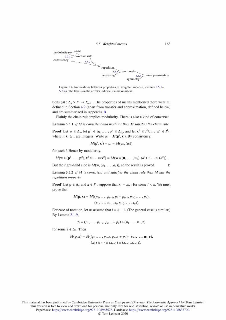
This material has been published by Cambridge University Press as Entropy and Diversity: The Axiomatic Approach by Tom Leinster.This version is free to view and download for personal use only. Not for re-distribution, re-sale or use in derivative works.
Paperback: https://www.cambridge.org/9781108965576. Hardback: https://www.cambridge.org/9781108832700.© Tom Leinster 2020
5.5 Weighted means 163
chain rule
repetition
increasing
transfer
symmetry
approximation
modularity
consistency
trivial
5.5.1
5.5.2
5.5.3
5.5.4
Figure 5.4 Implications between properties of weighted means (Lemmas 5.5.1–5.5.4). The labels on the arrows indicate lemma numbers.
tions (M : ∆n × In → I)n≥1. The properties of means mentioned there were alldefined in Section 4.2 (apart from transfer and approximation, defined below)and are summarized in Appendix B.
Plainly the chain rule implies modularity. There is also a kind of converse:
Lemma 5.5.1 If M is consistent and modular then M satisfies the chain rule.
Proof Let w ∈ ∆n, let p1 ∈ ∆k1 , . . . ,pn ∈ ∆kn , and let x1 ∈ Ik1 , . . . , xn ∈ Ikn ,where n, ki ≥ 1 are integers. Write ai = M(pi, xi). By consistency,
M(pi, xi) = ai = M(u1, (ai)
)for each i. Hence by modularity,
M(w (p1, . . . ,pn), x1 ⊕ · · · ⊕ xn) = M
(w (u1, . . . ,u1), (a1) ⊕ · · · ⊕ (an)
).
But the right-hand side is M(w, (a1, . . . , an)
), so the result is proved.
Lemma 5.5.2 If M is consistent and satisfies the chain rule then M has therepetition property.
Proof Let p ∈ ∆n and x ∈ In; suppose that xi = xi+1 for some i < n. We mustprove that
M(p, x) = M((p1, . . . , pi−1, pi + pi+1, pi+2, . . . , pn),
(x1, . . . , xi−1, xi, xi+2, . . . , xn)).
For ease of notation, let us assume that i = n − 1. (The general case is similar.)By Lemma 2.1.9,
p = (p1, . . . , pn−2, pn−1 + pn) (u1, . . . ,u1, r)
for some r ∈ ∆2. Then
M(p, x) = M((p1, . . . , pn−2, pn−1 + pn) (u1, . . . ,u1, r),
(x1) ⊕ · · · ⊕ (xn−2) ⊕ (xn−1, xn−1)),

This material has been published by Cambridge University Press as Entropy and Diversity: The Axiomatic Approach by Tom Leinster.This version is free to view and download for personal use only. Not for re-distribution, re-sale or use in derivative works.
Paperback: https://www.cambridge.org/9781108965576. Hardback: https://www.cambridge.org/9781108832700.© Tom Leinster 2020
164 Means
so by the chain rule and consistency,
M(p, x) = M((p1, . . . , pn−2, pn−1 + pn),(M(u1, (x1)), . . . ,M(u1, (xn−2)),M(r, (xn−1, xn−1))
))= M
((p1, . . . , pn−2, pn−1 + pn), (x1, . . . , xn−2, xn−1)
),
as required.
Lemma 5.5.3 If M has the repetition property and is increasing, then M alsohas the transfer property:
M(p, x) ≤ M((p1, . . . , pi−1, pi − δ, pi+1 + δ, pi+2, . . . , pn), x
)whenever 1 ≤ i < n, p ∈ ∆n, x ∈ In with xi ≤ xi+1, and 0 ≤ δ ≤ pi.
The transfer property states that a weighted mean increases when weight istransferred from a smaller argument to a larger one.
Proof As in the last proof, we may harmlessly assume that i = n− 1. We have
M(p, x) = M((p1, . . . , pn−2, pn−1 − δ, δ, pn), (x1, . . . , xn−2, xn−1, xn−1, xn)
)(5.45)
≤ M((p1, . . . , pn−2, pn−1 − δ, δ, pn), (x1, . . . , xn−2, xn−1, xn, xn)
)(5.46)
= M((p1, . . . , pn−2, pn−1 − δ, pn + δ), x
), (5.47)
where (5.45) and (5.47) hold by repetition and (5.46) holds because M is in-creasing.
Lemma 5.5.4 Suppose that M is symmetric and has the transfer property.Then M also has the following approximation property: for all p ∈ ∆n, x ∈ In
and δ > 0, there exist p−,p+ ∈ ∆n such that all the coordinates of p− and p+
are rational,
maxi|p−i − pi| < δ, max
i|p+
i − pi| < δ,
and
M(p−, x) ≤ M(p, x) ≤ M(p+, x).
Proof We just prove the existence of such a p+, the argument for p− beingsimilar. By symmetry, we may assume that x1 ≤ · · · ≤ xn.
Choose δ1 ∈ [0, δ) with 0 ≤ p1 − δ ∈ Q. By the transfer property,
M(p, x) ≤ M((p1 − δ1, p2 + δ1, p3, . . . , pn), x
).

This material has been published by Cambridge University Press as Entropy and Diversity: The Axiomatic Approach by Tom Leinster.This version is free to view and download for personal use only. Not for re-distribution, re-sale or use in derivative works.
Paperback: https://www.cambridge.org/9781108965576. Hardback: https://www.cambridge.org/9781108832700.© Tom Leinster 2020
5.5 Weighted means 165
Next, choose δ2 ∈ [0, δ) such that 0 ≤ p2 +δ1−δ2 ∈ Q. By the transfer property,
M((p1 − δ1, p2 + δ1, p3, . . . , pn), x
)≤ M
((p1 − δ1, p2 + δ1 − δ2, p3 + δ2, p4, . . . , pn), x
).
Continuing in this way, we obtain n − 1 inequalities that together imply that
M(p, x) ≤ M((p1 − δ1, p2 + δ1 − δ2, . . . , pn−1 + δn−2 − δn−1, pn + δn−1), x
).
The result follows by taking p+ to be the distribution on the right-hand side.
Many properties of weighted means M(−,−) imply the corresponding prop-erty of their unweighted counterparts M(un,−):
Lemma 5.5.5 Let I be an interval and let (M : ∆n × In → I)n≥1 be a sequenceof functions. If M is symmetric, consistent, increasing, or strictly increasing(respectively), then so is the sequence of functions
(M(un,−) : In → I
)n≥1.
Moreover, if I is closed under multiplication and M is homogeneous then so is(M(un,−))n≥1.
Proof Trivial.
It was stated on p. 144 that decomposability is an unweighted analogue ofthe chain rule. The following lemma supports that claim.
Lemma 5.5.6 Let I be a real interval and let (M : ∆n × In → I)n≥1 be asequence of functions that is consistent and satisfies the chain rule. Then(M(un,−) : In → I
)n≥1 is decomposable.
Proof Let n, k1, . . . , kn ≥ 1 and x1 ∈ Ik1 , . . . , xn ∈ Ikn . Write ai = M(uki , xi)and k =
∑ki. We must show that
M(uk, x1 ⊕ · · · ⊕ xn) = M(uk, (k1 ∗ a1, . . . , kn ∗ an)
).
We have
uk = (k1/k, . . . , kn/k) (uk1 , . . . ,ukn ),
so by the chain rule,
M(uk, x1 ⊕ · · · ⊕ xn) = M((k1/k, . . . , kn/k), (a1, . . . , an)
). (5.48)
But by Lemma 5.5.2, M has the repetition property, which implies by inductionthat the right-hand side of (5.48) is equal to
M(uk, (k1 ∗ a1, . . . , kn ∗ an)
).
This completes the proof.
This material has been published by Cambridge University Press as Entropy and Diversity: The Axiomatic Approach by Tom Leinster.This version is free to view and download for personal use only. Not for re-distribution, re-sale or use in derivative works.
Paperback: https://www.cambridge.org/9781108965576. Hardback: https://www.cambridge.org/9781108832700.© Tom Leinster 2020
166 Means
We now make a tool for converting theorems on unweighted means intotheorems on weighted means.
Proposition 5.5.7 Let I be a real interval and let(M,M′ : ∆n × In → I
)n≥1
be two sequences of functions. Suppose that:
i. both M and M′ have the absence-invariance and repetition properties;ii. M is symmetric and increasing;
iii. for each x ∈ In, the function M′(−, x) is continuous on the open simplex ∆n.
Suppose also that
M(un,−) = M′(un,−) : In → I
for all n ≥ 1. Then M = M′.
Proof First we prove that M(p,−) = M′(p,−) when the coordinates of p arerational and nonzero. Write
p = (k1/k, . . . , kn/k),
where k1, . . . , kn are positive integers and k =∑
ki. Let x ∈ In. Then by therepetition property of M and induction,
M(p, x) = M(uk, (k1 ∗ x1, . . . , kn ∗ xn)
). (5.49)
The same argument applied to M′ gives
M′(p, x) = M′(uk, (k1 ∗ x1, . . . , kn ∗ xn)
). (5.50)
But the right-hand sides of (5.49) and (5.50) are equal by hypothesis, soM(p, x) = M′(p, x).
Now we show by induction on n ≥ 1 that M(p, x) = M′(p, x) for all p ∈ ∆n
and x ∈ In.For n = 1, we must have p = u1, hence M(p, x) = M′(p, x) by hypothesis.Let n ≥ 2 and assume the result for n − 1. If pi = 0 for some i then
M(p, x) = M′(p, x) by inductive hypothesis and absence-invariance of M andM′. Suppose, then, that p ∈ ∆n.
Let ε > 0. Since M′(−, x) is continuous at p, we can choose δ ∈ (0,mini pi)such that for r ∈ ∆n,
maxi|pi − ri| < δ =⇒ |M′(p, x) − M′(r, x)| < ε.

This material has been published by Cambridge University Press as Entropy and Diversity: The Axiomatic Approach by Tom Leinster.This version is free to view and download for personal use only. Not for re-distribution, re-sale or use in derivative works.
Paperback: https://www.cambridge.org/9781108965576. Hardback: https://www.cambridge.org/9781108832700.© Tom Leinster 2020
5.5 Weighted means 167
By Lemma 5.5.3, M has the transfer property, so by Lemma 5.5.4, M also hasthe approximation property. Choose p+ as in Lemma 5.5.4; then
|M′(p, x) − M′(p+, x)| < ε. (5.51)
Also, since p ∈ ∆n and
maxi|pi − p+
i | < δ < mini
pi,
we have p+ ∈ ∆n too. Now
M(p, x) ≤ M(p+, x) (5.52)
= M′(p+, x) (5.53)
< M′(p, x) + ε, (5.54)
where inequality (5.52) is one of the defining properties of p+, equation (5.53)holds because the coordinates of p+ are rational and nonzero (using the firststep of the proof), and inequality (5.54) follows from (5.51). But this holds forall ε > 0, so
M(p, x) ≤ M′(p, x).
A very similar argument, using the distribution p− of Lemma 5.5.4, proves theopposite inequality. Hence M(p, x) = M′(p, x), completing the proof.
We can now simply read off four characterization theorems for weightedpower means. They are summarized in Table 5.2, and are derived from thefour theorems on unweighted means shown in Table 5.1.
Theorem 5.5.8 Let(M : ∆n×(0,∞)n → (0,∞)
)n≥1 be a sequence of functions.
The following are equivalent:
i. M is symmetric, absence-invariant, consistent, strictly increasing, modular,and homogeneous;
ii. M = Mt for some t ∈ (−∞,∞).
Proof Part (ii) implies part (i) by the results in Section 4.2. Now assume (i).The unweighted mean (
M(un,−) : (0,∞)n → (0,∞))n≥1
is symmetric, strictly increasing, decomposable, and homogeneous (usingLemmas 5.5.1 and 5.5.6 for decomposability). Hence by Theorem 5.3.2, thereis some t ∈ (−∞,∞) such that
M(un,−) = Mt(un,−)

This material has been published by Cambridge University Press as Entropy and Diversity: The Axiomatic Approach by Tom Leinster.This version is free to view and download for personal use only. Not for re-distribution, re-sale or use in derivative works.
Paperback: https://www.cambridge.org/9781108965576. Hardback: https://www.cambridge.org/9781108832700.© Tom Leinster 2020
168 Means
for all n ≥ 1. By Lemmas 5.5.1 and 5.5.2, M has the repetition property. Henceby the previously-established properties of Mt, we can apply Proposition 5.5.7with M′ = Mt, giving M = Mt.
Theorem 5.5.8 is essentially due to Hardy, Littlewood and Polya [135].Some minor details aside, it is the conjunction of their Theorems 84 and 215,translated out of the language of Stieltjes integrals and into elementary terms.Section 6.21 of [135] gives details.
Theorem 5.5.9 Let(M : ∆n× [0,∞)n → [0,∞)
)n≥1 be a sequence of functions.
The following are equivalent:
i. M is symmetric, absence-invariant, consistent, strictly increasing, modular,and homogeneous;
ii. M = Mt for some t ∈ (0,∞).
Proof This follows by exactly the same argument as for the last theorem, butusing Theorem 5.3.3 instead of Theorem 5.3.2.
Theorem 5.5.10 Let(M : ∆n × (0,∞)n → (0,∞)
)n≥1 be a sequence of func-
tions. The following are equivalent:
i. M is symmetric, absence-invariant, consistent, increasing, modular, andhomogeneous;
ii. M = Mt for some t ∈ [−∞,∞].
Proof This follows from Theorem 5.4.7 by the same argument.
Theorem 5.5.11 Let(M : ∆n × [0,∞)n → [0,∞)
)n≥1 be a sequence of func-
tions. The following are equivalent:
i. M is symmetric, absence-invariant, consistent, increasing, modular, homo-geneous, and continuous in its second argument;
ii. M = Mt for some t ∈ [−∞,∞].
Proof This follows from Theorem 5.4.9 by the same argument again, this timealso noting that by consistency, none of the functions M(un,−) is identicallyzero.
We will use Theorem 5.5.10 to prove an axiomatic characterization of mea-sures of the value of a community (Section 7.3) and, building on this, to char-acterize the Hill numbers (Section 7.4).
This material has been published by Cambridge University Press as Entropy and Diversity: The Axiomatic Approach by Tom Leinster.This version is free to view and download for personal use only. Not for re-distribution, re-sale or use in derivative works.
Paperback: https://www.cambridge.org/9781108965576. Hardback: https://www.cambridge.org/9781108832700.© Tom Leinster 2020
6
Species similarity and magnitude
Alfred Russel Wallace, who in parallel with Charles Darwin discovered whatwe now call the theory of evolution, spent much of the 1850s travelling intropical south-east Asia and South America. On his return, he wrote widely onwhat he had experienced, including the following description of the diversityof a tropical forest ([343], p. 65):
If the traveller notices a particular species and wishes to find more likeit, he may often turn his eyes in vain in every direction. Trees of variedforms, dimensions, and colours are around him, but he rarely sees any oneof them repeated. Time after time he goes towards a tree which looks likethe one he seeks, but a closer examination proves it to be distinct. He mayat length, perhaps, meet with a second specimen half a mile off, or mayfail altogether, till on another occasion he stumbles on one by accident.
One of Wallace’s observations was that besides there being a large number ofspecies, mostly rare, there was also a great deal of similarity between differentspecies. Clearly, any comprehensive account of the variety or diversity of lifehas to incorporate the varying degrees of similarity between species. All elsebeing equal, a community of species that are closely related to one anothershould be judged as less diverse than if they were highly dissimilar.
This is not an abstract concern. The Organization for Economic Co-operation and Development’s guide to biodiversity for policy makers recog-nizes this same point, stating that
associated with the idea of diversity is the concept of distance, i.e., somemeasure of the dissimilarity of the resources in question
([265], p. 25). With global biodiversity now being lost at historically unprece-dented rates, it is crucial that politicians and scientists speak the same lan-guage. However, most conventional measures of diversity, and all the ones
169

This material has been published by Cambridge University Press as Entropy and Diversity: The Axiomatic Approach by Tom Leinster.This version is free to view and download for personal use only. Not for re-distribution, re-sale or use in derivative works.
Paperback: https://www.cambridge.org/9781108965576. Hardback: https://www.cambridge.org/9781108832700.© Tom Leinster 2020
170 Species similarity and magnitude
discussed in this text so far, fail to take the different dissimilarities betweenspecies into account.
Here we solve this problem, defining a system of measures that depend notonly on the relative abundances of the species, but also on the varying similar-ity between them (Sections 6.1 and 6.2). It was first introduced in a 2012 articleof Leinster and Cobbold [218]. We make no assumption about how similarityis measured: it could be genetic, phylogenetic, functional, etc., leading to mea-sures of genetic diversity, phylogenetic diversity, functional diversity, etc. Assuch, the system is adaptable to a wide variety of scientific needs.
More specifically, we will encode the similarities between species as a realmatrix Z, continuing to represent the relative abundances of the species as aprobability distribution p. With this model of a community, we will define foreach q ∈ [0,∞] a measure DZ
q (p) of the diversity of the community. As forthe Hill numbers, the parameter q controls the extent to which the measureemphasizes the common species at the expense of the rare ones. Under theextreme hypothesis that different species never have anything in common, Z isthe identity matrix I and the diversity DI
q(p) reduces to the Hill number Dq(p).In that sense, these similarity-sensitive diversity measures generalize the Hillnumbers.
Let p be a probability distribution on a finite set. We saw in Section 4.3that the Hill numbers Dq(p), the Renyi entropies Hq(p) and the q-logarithmicentropies S q(p) are all simple increasing transformations of one another.The same is true in the more general context here. Thus, accompanying thesimilarity-sensitive diversity measures DZ
q (p) are similarity-sensitive Renyi en-tropies HZ
q (p) and q-logarithmic entropies S Zq (p). Any metric on our finite set
gives rise naturally to a similarity matrix Z, as we shall see. So, we obtain def-initions of the Renyi and q-logarithmic entropies of a probability distributionon a finite metric space, extending the classical definitions on a finite set.
How is diversity maximized? For a fixed similarity matrix Z (and in par-ticular, for a finite metric space), we can seek the probability distribution pthat maximizes the diversity or entropy of a given order q. As we saw in thespecial case of the Hill numbers, different values of q can lead to differentjudgements on which of two communities is the more diverse. So in principle,both the maximizing distribution and the value of the maximum diversity de-pend on q. However, it is a theorem that neither does. Every similarity matrixhas an unambiguous maximum diversity, independent of q, and a distributionthat maximizes the diversity of all orders q simultaneously. This is the subjectof Section 6.3.
The maximum diversity of a matrix Z is closely related to another quantity,the magnitude of a matrix. The general concept of magnitude, expressed in

This material has been published by Cambridge University Press as Entropy and Diversity: The Axiomatic Approach by Tom Leinster.This version is free to view and download for personal use only. Not for re-distribution, re-sale or use in derivative works.
Paperback: https://www.cambridge.org/9781108965576. Hardback: https://www.cambridge.org/9781108832700.© Tom Leinster 2020
6.1 The importance of species similarity 171
the formalism of enriched categories, brings together a wide range of size-likeinvariants in mathematics, including cardinality, Euler characteristic, volume,surface area, dimension, and other geometric measures. Sections 6.4 and 6.5are a broad-brush survey of magnitude, and demonstrate that maximum di-versity – far from being tethered to ecology – has profound connections withfundamental invariants of geometry.
6.1 The importance of species similarity
Here we introduce a family of measures of the diversity of an ecological com-munity that take into account the varying similarities between species, follow-ing work of Leinster and Cobbold [218].
These diversity measures will be almost completely neutral as to what ‘sim-ilarity’ means or how it is quantified, just as the diversity measures discussedearlier were neutral as to the meaning of abundance (Example 2.1.1). The fol-lowing examples illustrate some of the ways in which similarity can be quan-tified. In these examples, the similarity z between two species is measured ona scale of 0 to 1, with 0 representing complete dissimilarity and 1 representingidentical species.
Examples 6.1.1 i. The similarity z between two species can be interpreted aspercentage genetic similarity (in any of several senses; typically one wouldrestrict to a particular part of the genome). With the rapid fall in the costof DNA sequencing, this way of quantifying similarity is increasingly com-mon. It can be used even when the taxonomic classification of the organ-isms concerned is unclear or incomplete, as is often the case for microbialcommunities (a problem discussed by Johnson [159] and Watve and Gan-gal [346], for instance).
ii. Functional similarity can also be quantified. For instance, suppose that wehave a list of k functional traits satisfied by some species but not others.We can then define the similarity z between two species as j/k, where jis the number of traits possessed by either both species or neither. (For anoverview of functional diversity, see Petchey and Gaston [277].)
iii. Similarity can also be measured phylogenetically, that is, in terms of anevolutionary tree. For instance, z can be defined as the proportion of evo-lutionary time before the two species diverged, relative to some fixed starttime.
iv. In the absence of better data, we can measure similarity crudely using tax-onomy. For instance, we could define the similarity z between two species

This material has been published by Cambridge University Press as Entropy and Diversity: The Axiomatic Approach by Tom Leinster.This version is free to view and download for personal use only. Not for re-distribution, re-sale or use in derivative works.
Paperback: https://www.cambridge.org/9781108965576. Hardback: https://www.cambridge.org/9781108832700.© Tom Leinster 2020
172 Species similarity and magnitude
by
z =
1 if the species are the same,
0.8 if the species are different but of the same genus,
0.5 if the species are of different genera but the same family,
0 otherwise,
or similarly for any other choice of constants and number of taxonomiclevels.
v. More crudely still, we can define the similarity z between two species by
z =
1 if the species are the same,
0 if the species are different.
This definition embodies the assumption that different species never haveanything in common. Unrealistic as this is, we will see that it is implicit inall of the measures of diversity defined in this book so far, and most of thediversity measures common in the ecological literature.
Now consider a list of species, numbered as 1, . . . , n, and suppose that wehave fixed a way of quantifying the similarity between them. We obtain an n×nmatrix
Z =(Zi j
)1≤i, j≤n,
where Zi j is the similarity between species i and j.Formally, a real square matrix Z is a similarity matrix if Zi j ≥ 0 for all
i, j and Zii > 0 for all i. The examples above suggest additional hypotheses:that Zi j ≤ 1 for all i, j, that Zii = 1 for all i, and that Z is symmetric. (Indeed,in the paper [218] on which this section is based, the term ‘similarity matrix’included the first two of these additional hypotheses.) But in most of whatfollows, we will not need these extra assumptions, so we do not make them.
Examples 6.1.2 i. The genetic, functional, phylogenetic and taxonomic sim-ilarity measures of Examples 6.1.1 give genetic, functional, phylogeneticand taxonomic similarity matrices Z, taking Zi j to be any of the quantities zdescribed there.
ii. The very crude similarities z of Example 6.1.1(v), where distinct species aretaken to be completely dissimilar, give the identity similarity matrix Z = I.We will call this the naive model of a community.
Example 6.1.3 Given any finite metric space, with distance d and points la-belled as 1, . . . , n, we obtain an n × n similarity matrix Z by setting
Zi j = e−d(i, j).

This material has been published by Cambridge University Press as Entropy and Diversity: The Axiomatic Approach by Tom Leinster.This version is free to view and download for personal use only. Not for re-distribution, re-sale or use in derivative works.
Paperback: https://www.cambridge.org/9781108965576. Hardback: https://www.cambridge.org/9781108832700.© Tom Leinster 2020
6.1 The importance of species similarity 173
Thus, large distances correspond to small similarities. In the extreme, the met-ric defined by d(i, j) = ∞ for all i , j corresponds to the naive model. (Weallow∞ as a distance in our metric spaces.) Any taxonomic similarity matrix ofthe general type indicated in Example 6.1.1(iv) corresponds to an ultrametricspace, that is, a metric space satisfying the stronger form
d(i, k) ≤ maxd(i, j), d( j, k)
of the triangle inequality.From a purely mathematical viewpoint, this matrix Z =
(e−d(i, j)) associated
with a finite metric space is highly significant, as we will discover when wecome to the theory of magnitude (Sections 6.4 and 6.5). From a biologicalviewpoint, we may find ourselves starting with a measure of inter-species dif-ference δ on a scale of 0 to ∞ (as in Warwick and Clarke [345], for instance),in which case the transformation z = e−δ converts it into a similarity z on ascale of 0 to 1. From both viewpoints, the choice of constant e is arbitrary, andone should consider replacing it by any other constant, or equivalently, scalingthe distance by a linear factor. Again, this is a fundamental point in the theoryof magnitude, as demonstrated by the theorems in Section 6.5.
Example 6.1.4 A symmetric similarity matrix whose entries are all 0 or 1 cor-responds to a finite reflexive graph with no multiple edges. Here, reflexivemeans that there is an edge from each vertex to itself (a loop). The correspon-dence works as follows: labelling the vertices of the graph as 1, . . . , n, we putZi j = 1 whenever there is an edge between i and j, and Zi j = 0 otherwise. Onesays that Z is the adjacency matrix of the graph. The reflexivity means thatZii = 1 for all i.
No ecological relevance is claimed for this family of examples, but mathe-matically it is a natural special case, and it sheds light on computational aspectsof calculating maximum diversity (Remark 6.3.24).
Our earlier discussions of diversity modelled an ecological communitycrudely as a finite probability distribution p = (p1, . . . , pn). Our new and lesscrude model of a community has two components: a relative abundance dis-tribution p ∈ ∆n and an n × n similarity matrix Z. We now build up to thedefinition of the diversity of a community modelled in this way.
Treating p as a column vector, we can form the matrix product Zp, whichhas entries
(Zp)i =
n∑j=1
Zi j p j (6.1)
(1 ≤ i ≤ n). The quantity (6.1) is the expected similarity between an individual

This material has been published by Cambridge University Press as Entropy and Diversity: The Axiomatic Approach by Tom Leinster.This version is free to view and download for personal use only. Not for re-distribution, re-sale or use in derivative works.
Paperback: https://www.cambridge.org/9781108965576. Hardback: https://www.cambridge.org/9781108832700.© Tom Leinster 2020
174 Species similarity and magnitude
of species i and an individual chosen at random. It can therefore be understoodas the ordinariness of species i. If the diagonal entries of Z are all 1 (as in everyexample above) then
(Zp)i =∑
j
Zi j p j ≥ Zii pi = pi. (6.2)
This inequality states that a species appears more ordinary when the similari-ties between species are recognized than when they are ignored.
By inequality (6.2), any species that is highly abundant is also highly ordi-nary: large pi implies large (Zp)i. But even if species i is rare, its ordinariness(Zp)i will be high if there is some common species very similar to it. The or-dinariness of species i will even be high if it is similar to several species thatare each individually rare, but whose total abundance is large. (For example,in Wallace’s tropical forest, many tree species have much higher ordinariness(Zp)i than relative abundance pi.) This makes intuitive sense: the more thornybushes a region contains, the more ordinary any thorny bush will seem, even ifits particular species is rare.
Judgements about what is ‘ordinary’ depend on one’s perception of similar-ity. If one wishes to make a strong distinction between different species, oneshould use a similarity matrix Z whose off-diagonal entries are small, and thiswill have the effect of lowering the ordinariness of every species.
Since (Zp)i measures how ordinary the ith species is, 1/(Zp)i measures howspecial it is. In the case Z = I (the naive model of Example 6.1.2(ii)), thisreduces to 1/pi, which in Sections 2.4 and 4.3 we called the specialness orrarity of species i. We have now extended that concept to our more refinedmodel.
When we modelled a community as a simple probability distribution, wedefined the diversity of a community to be the average specialness of an indi-vidual within it. We do the same again now in our new model.
Definition 6.1.5 Let p ∈ ∆n, let Z be an n × n similarity matrix, and let q ∈[0,∞]. The diversity of p of order q, with respect to Z, is
DZq (p) = M1−q(p, 1/Zp).
Here, the vector 1/Zp is defined as(1/(Zp)1, . . . , 1/(Zp)n
).
Although there may be some values of i for which (Zp)i = 0, this can onlyoccur when pi = 0: for Zii > 0 by definition of similarity matrix, so if pi > 0

This material has been published by Cambridge University Press as Entropy and Diversity: The Axiomatic Approach by Tom Leinster.This version is free to view and download for personal use only. Not for re-distribution, re-sale or use in derivative works.
Paperback: https://www.cambridge.org/9781108965576. Hardback: https://www.cambridge.org/9781108832700.© Tom Leinster 2020
6.1 The importance of species similarity 175
then
(Zp)i =∑
j
Zi j p j ≥ Zii pi > 0.
So by the convention in Remark 4.2.15, M1−q(p, 1/Zp) is well-defined. Explic-itly,
DZq (p) =
( ∑i∈supp(p)
pi(Zp)q−1i
)1/(1−q)
for q , 1,∞, and
DZ1 (p) =
∏i∈supp(p)
(Zp)−pii =
1(Zp)p1
1 · · · (Zp)pnn,
DZ∞(p) =
1max
i∈supp(p)(Zp)i
.
We could extend Definition 6.1.5 to negative q, but it would be misleadingto call DZ
q (p) ‘diversity’ when q is negative, for the reasons given in Re-mark 4.4.4(ii). We therefore restrict to q ∈ [0,∞].
Examples 6.1.6 Here we consider some special values of Z and q, and in do-ing so recover various earlier measures of diversity.
i. In the naive model Z = I, where distinct species are taken to be completelydissimilar, Zp = p and so DZ
q (p) is just the Hill number Dq(p). In this sense,the Hill numbers implicitly use the naive model of a community.
ii. For a general similarity matrix, the diversity of order 0 is
DZ0 (p) =
∑i∈supp(p)
pi
(Zp)i.
This is a sum of contributions from all species present. The contributionmade by the ith species, pi/(Zp)i, is between 0 and 1, by inequality (6.2)(assuming that Zii = 1). It is large when, relative to the size of the ithspecies, there are not many individuals of other similar species – that is,when the ith species is unusual. We discuss the quantity pi/(Zp)i in greaterdepth in Example 7.1.7.
iii. In the naive model, the diversity of order∞ is the Berger–Parker index
DI∞(p) = D∞(p) = 1
/max
ipi
(Example 4.3.5(iv)). It measures the dominance of the most common

This material has been published by Cambridge University Press as Entropy and Diversity: The Axiomatic Approach by Tom Leinster.This version is free to view and download for personal use only. Not for re-distribution, re-sale or use in derivative works.
Paperback: https://www.cambridge.org/9781108965576. Hardback: https://www.cambridge.org/9781108832700.© Tom Leinster 2020
176 Species similarity and magnitude
species, the idea being that in a diverse community, no species should betoo dominant. For a general similarity matrix, the diversity
DZ∞(p) = 1
/max
i∈supp(p)(Zp)i
of order ∞ can be interpreted in the same way, but now with sensitivity tospecies similarity: DZ
∞(p) is low not only if there is a single highly abundantspecies, but also if there is some highly abundant cluster of species.
iv. The diversity of order 2 is
DZ2 (p) = 1
/ n∑i, j=1
piZi j p j = 1/pTZp.
(We continue to regard p as a column vector, so that its transpose pT is arow vector.) The number pTZp is the expected similarity between a pair ofindividuals chosen at random. This is a measure of a community’s lack ofdiversity, and its reciprocal DZ
2 (p) therefore measures diversity itself.For instance, take a probability distribution p on the vertices of a graph,
and let Z be the adjacency matrix (as in Example 6.1.4). Then DZ2 (p) is the
reciprocal of the probability that two vertices chosen at random are adja-cent (joined by an edge). Equivalently, if pairs of vertices are repeatedlychosen at random, DZ
2 (p) is the expected number of trials needed in orderto find an adjacent pair.
Example 6.1.7 By Example 6.1.6(iv), one can estimate the diversity of or-der 2 of a community by sampling pairs of individuals at random, recordingthe similarity between them, calculating the mean of these similarities, thentaking the reciprocal. More generally, for any integer q ≥ 2, one can estimateDZ
q (p) as follows. Sample q individuals at random from the community (withreplacement). Supposing that they are of species i1, . . . , iq, let us temporarilyrefer to the product
Zi1i2 Zi1i3 · · · Zi1iq
as their ‘group similarity’. Let µq be the expected group similarity of q indi-viduals from the community. Then
DZq (p) = µ
1/(1−q)q .
This was first proved as Proposition A3 of the appendix to [218], and the proofis also given here as Appendix A.5.
For instance, in the naive model, µq is the probability that q random individ-uals are all of the same species, which is
∑i pq
i . In this case, it is immediatethat Dq(p) = µ
1/(1−q)q .
This material has been published by Cambridge University Press as Entropy and Diversity: The Axiomatic Approach by Tom Leinster.This version is free to view and download for personal use only. Not for re-distribution, re-sale or use in derivative works.
Paperback: https://www.cambridge.org/9781108965576. Hardback: https://www.cambridge.org/9781108832700.© Tom Leinster 2020
6.1 The importance of species similarity 177
This procedure for estimating the diversity of orders 2, 3, . . . has the advan-tage that it does not require the organisms to be classified into species. All werequire is a measure of similarity between any pair of individuals. This is po-tentially very useful in studies of microbial systems, where there is often nocomplete taxonomic classification; all we have is a way of measuring the sim-ilarity between two samples. We can estimate µq, hence DZ
q (p), by repeatedlydrawing q samples from the community, recording their group similarity, andthen taking the mean.
Both relative abundance and similarity can be quantified in whatever wayis appropriate to the scientific problem at hand. This makes the diversity mea-sures DZ
q (p) highly versatile. For example, if the similarity coefficients Zi j aredefined genetically then DZ
q measures genetic diversity, and in the same way,a phylogenetic, functional or taxonomic similarity matrix will produce a mea-sure of phylogenetic, functional or taxonomic diversity.
The different diversity measures arising from different choices of similaritymatrix may produce opposing results. This is a feature, not a bug. For instance,if over a period of time, a community undergoes an increase in genetic diversitybut a decrease in morphological diversity, the opposite trends are a point ofscientific interest.
When selecting a similarity matrix, a useful observation is that if
Z =
(1 zz 1
)then
DZq( 1
2 ,12)
=2
1 + z,
or equivalently
z =2
DZq( 1
2 ,12) − 1,
for all q ∈ [0,∞]. So, deciding on the similarity Zi j between species i and j isequivalent to deciding on the diversity d of a community consisting of speciesi and j in equal proportions:
Zi j =2d− 1.
Taking d = 1 embodies the viewpoint that this two-species community con-sists of effectively only one species, giving a similarity coefficient Zi j = 1: thespecies are deemed to be identical. At the opposite extreme, if one decides that

This material has been published by Cambridge University Press as Entropy and Diversity: The Axiomatic Approach by Tom Leinster.This version is free to view and download for personal use only. Not for re-distribution, re-sale or use in derivative works.
Paperback: https://www.cambridge.org/9781108965576. Hardback: https://www.cambridge.org/9781108832700.© Tom Leinster 2020
178 Species similarity and magnitude
Species Abundance Abundancein canopy in understorey
Prepona laertes 15 0Archaeoprepona demophon 14 37Zaretis itys 25 11Memphis arachne 89 23Memphis offa 21 3Memphis xenocles 32 8
Table 6.1 Counts of butterflies of species in the subfamily Charaxinae, in thecanopy and understorey of an Ecuadorian rain forest site (Example 6.1.8; datafrom Table 5 of DeVries et al. [81]).
such a community should have diversity 2 (‘effectively 2 species’) for all i andj, this produces the naive matrix Z = I.
The flexibility afforded by the choice of similarity matrix may make it tempt-ing to reject the measures DZ
q in favour of the simpler Hill numbers Dq, whereno such choice is necessary. However, it is a mathematical fact that doing soamounts to choosing the naive model Z = I (Example 6.1.6(i)), which rep-resents the extreme position that distinct species have nothing whatsoever incommon. This always leads to an overestimate of diversity (Lemma 6.2.3).The framework of similarity matrices forces us to be transparent: using thenaive similarity matrix I is a choice, embodying ecological assumptions, justas much as for any other similarity matrix.
The next example, adapted from [218] (Example 3), demonstrates how eco-logical judgements can be altered by taking species similarity into account.Extending the terminology of Chapter 4, we refer to the graph of DZ
q (p) againstq as a diversity profile.
Example 6.1.8 DeVries et al. ([81], Table 5) counted butterflies in the canopyand understorey at a certain site in the Ecuadorian rain forest. In the subfamilyCharaxinae, the abundances were as shown in Table 6.1. We will compare thediversity profiles of the canopy and the understorey in two ways, once usingthe naive similarity matrix and once using a non-naive matrix.
With the naive similarity matrix I, the diversity profiles are as shown inFigure 6.1(a). The profile of the canopy lies above that of the understorey un-til about q = 5, after which the two profiles are near-identical. So, whateveremphasis we may place on rare or common species, the canopy is at least asdiverse as the understorey.
Now let us compare the communities using a taxonomic similarity matrix.

This material has been published by Cambridge University Press as Entropy and Diversity: The Axiomatic Approach by Tom Leinster.This version is free to view and download for personal use only. Not for re-distribution, re-sale or use in derivative works.
Paperback: https://www.cambridge.org/9781108965576. Hardback: https://www.cambridge.org/9781108832700.© Tom Leinster 2020
6.1 The importance of species similarity 179
2
3
4
5
6
0 1 2 3 4 5
CanopyUnderstorey
Viewpoint parameter, q
Div
ersi
ty,D
q(p)
(a) Naive similarity
2
3
4
5
6
0 1 2 3 4 5
CanopyUnderstorey
Viewpoint parameter, q
Div
ersi
ty,D
Z q(p
)
(b) Taxonomic similarity
Figure 6.1 Diversity profiles of butterflies in the canopy and understorey of arain forest site, using (a) the naive similarity matrix I; (b) a taxonomic similaritymatrix. Graphs adapted from Figure 3 of Leinster and Cobbold [218].
Put
Zi j =
1 if i = j,
0.5 if species i and j are different but of the same genus,
0 otherwise.
The resulting diversity profiles, shown in Figure 6.1(b), tell a different story.For most values of q, it is the understorey that is more diverse. This canbe explained as follows. Most of the canopy population belongs to the threespecies in the Memphis genus, so when we build into the model the principlethat species of the same genus tend to be somewhat similar, the canopy looksless diverse than it did before. On the other hand, the understorey populationdoes not contain large numbers of individuals of different species but the samegenus, so factoring in taxonomic similarity does not cause its diversity to de-crease so much.
The measures DZq , as well as unifying into one family many older diver-
sity measures, have also found application in a variety of ecological systems atmany scales, from microbes (Bakker et al. [26]), fungi (Veresoglou et al. [341])and crustacean zooplankton (Jeziorski et al. [158]) to alpine plants (Chalman-drier et al. [64]) and large arctic predators (Bromaghin et al. [50]). As onewould expect, incorporating similarity has been found to improve inferencesabout the diversity of natural systems [341]. The measures have also been ap-

This material has been published by Cambridge University Press as Entropy and Diversity: The Axiomatic Approach by Tom Leinster.This version is free to view and download for personal use only. Not for re-distribution, re-sale or use in derivative works.
Paperback: https://www.cambridge.org/9781108965576. Hardback: https://www.cambridge.org/9781108832700.© Tom Leinster 2020
180 Species similarity and magnitude
plied in non-biological contexts such as computer network security (Wang etal. [344]).
We now turn from diversity to entropy. In the simpler context of probabilitydistributions p on a finite set, we defined three closely related quantities foreach parameter value q: the Hill number Dq(p), the Renyi entropy Hq(p), andthe q-logarithmic entropy S q(p). They are related to one another by increasing,invertible transformations:
Hq(p) = log Dq(p),
S q(p) = lnq Dq(p)
(equations (4.20)). Given also a similarity matrix Z, we define the similarity-sensitive Renyi entropy HZ
q (p) and similarity-sensitive q-logarithmic en-tropy S Z
q (p) by the same transformations:
HZq (p) = log DZ
q (p), (6.3)
S Zq (p) = lnq DZ
q (p). (6.4)
In the first definition, q ∈ [0,∞], and in the second, q ∈ [0,∞).Let us be explicit. For q , 1,∞, the similarity-sensitive Renyi entropy is
HZq (p) =
11 − q
log∑
i∈supp(p)
pi(Zp)q−1i ,
and in the exceptional cases,
HZ1 (p) = −
∑i∈supp(p)
pi log(Zp)i
(generalizing the Shannon entropy) and
HZ∞(p) = − log max
i∈supp(p)(Zp)i.
We now derive an explicit expression for S Zq (p). By Lemma 4.2.29,
S Zq (p) = lnq M1−q(p, 1/Zp) =
∑i∈supp(p)
pi lnq1
(Zp)i.
Then applying the definition of lnq gives
S Zq (p) =
11 − q
( ∑i∈supp(p)
pi(Zp)q−1i − 1
)when q , 1, and
S Z1 (p) = HZ
1 (p) = −∑
i∈supp(p)
pi log(Zp)i.
This material has been published by Cambridge University Press as Entropy and Diversity: The Axiomatic Approach by Tom Leinster.This version is free to view and download for personal use only. Not for re-distribution, re-sale or use in derivative works.
Paperback: https://www.cambridge.org/9781108965576. Hardback: https://www.cambridge.org/9781108832700.© Tom Leinster 2020
6.1 The importance of species similarity 181
Figure 4.1, which schematically depicts the two families of deformed entropiesin the special case Z = I, applies equally to an arbitrary similarity matrix Z.
Example 6.1.9 The definitions above specialize to definitions of Renyi andq-logarithmic entropies for a probability distribution on a finite metric space.Indeed, let A = 1, . . . , n be a finite metric space and write Z =
(e−d(i, j)), as in
Example 6.1.3. For any probability distribution p on A, and for any parametervalue q, we have an associated Renyi entropy HZ
q (p) and q-logarithmic entropyS Z
q (p). Naturally, these quantities depend on the metric. In the extreme casewhere d(i, j) = ∞ for all i , j, we recover the standard definitions of the Renyiand q-logarithmic entropies of a probability distribution on a finite set.
(One can speculate about extending the results of classical information the-ory to the metric context. As usual, the elements of the set A = 1, . . . , nrepresent the source symbols and the distribution p specifies their frequencies,but now we also have a metric d on the source symbols. It could be defined insuch a way that d(i, j) is small when the ith and jth symbols are easily mis-taken for one another, or alternatively when one is an acceptable substitute forthe other, for applications such as the encoding of colour images.)
Example 6.1.10 For any similarity matrix Z, we can define a dissimilaritymatrix ∆ by ∆i j = 1 − Zi j. (Let us assume here that Zi j ≤ 1 for all i and j.) Inthese terms, the 2-logarithmic entropy is
S Z2 (p) = 1 −
∑i, j
piZi j p j =∑i, j
pi∆i j p j = pT∆p.
Thus, S Z2 (p) is the dissimilarity between a pair of individuals chosen at random.
This quantity, studied by the statistician C. R. Rao [283, 284], is known asRao’s quadratic entropy.
Of course, anything that can be expressed in terms of Z can also be expressedin terms of ∆, and vice versa. An important early step towards similarity-sensitive diversity measures was taken by Ricotta and Szeidl [293], who gavea version of the entropy S Z
q (p) expressed in terms of a dissimilarity matrix ∆.
Example 6.1.11 Let Z be the adjacency matrix of a finite reflexive graph Gwith vertex-set 1, . . . , n, as in Example 6.1.4. Write i ∼ j to mean that verticesi and j are joined by an edge, and i 6∼ j otherwise. Then the dissimilarity matrix∆ of the last example has entries 1 for non-adjacent pairs and 0 for adjacentpairs. Hence the 2-logarithmic entropy of a probability distribution p on G isgiven by
S Z2 (p) =
∑i, j : i 6∼ j
pi p j.
This material has been published by Cambridge University Press as Entropy and Diversity: The Axiomatic Approach by Tom Leinster.This version is free to view and download for personal use only. Not for re-distribution, re-sale or use in derivative works.
Paperback: https://www.cambridge.org/9781108965576. Hardback: https://www.cambridge.org/9781108832700.© Tom Leinster 2020
182 Species similarity and magnitude
This is the probability that two vertices chosen at random according to p arenot joined by an edge. Thus, entropy is high when vertices of high probabilitytend not to be adjacent. We will make more precise statements of this type inSection 6.3, where we will solve the problem of maximizing entropy on a setwith similarities – and, in particular, maximizing entropy on a graph.
6.2 Properties of the similarity-sensitive diversity measures
Here we establish the algebraic and analytic properties of the similarity-sensitive diversity measures DZ
q (p), extending the results already proved inSection 4.4 for the Hill numbers (the case Z = I). Mathematically speaking,most of the properties of the diversity measures are easy consequences of theproperties of means. However, they are given new significance by the ecologi-cal interpretation.
Each of the listed properties of DZq (p) is a piece of evidence that these mea-
sures behave logically, in the way that should be required of any diversitymeasure. Contrast, for instance, the behaviour of Shannon entropy in the oilcompany argument of Example 2.4.11. Nearly all of the properties were firstestablished in the 2012 paper of Leinster and Cobbold [218].
In the naive model, diversity profiles are either strictly decreasing or constant(Proposition 4.4.1), and we will show that this is also true in general case. Butwhereas in the naive model, the condition for the profile to be constant is thatall species present have equal abundance pi, in the general case, the conditionis that all species present have equal ordinariness (Zp)i .
Proposition 6.2.1 Let Z be an n × n similarity matrix and let p ∈ ∆n. ThenDZ
q (p) is a decreasing function of q ∈ [0,∞]. It is constant if (Zp)i = (Zp) j forall i, j ∈ supp(p), and strictly decreasing otherwise.
Proof Since DZq (p) = M1−q(p, 1/Zp), this follows from Theorem 4.2.8.
The more similar the species in a population are perceived to be, the less theperceived diversity. Our diversity measures conform to this intuition:
Lemma 6.2.2 Let Z′ and Z be n × n similarity matrices with Z′i j ≤ Zi j for alli, j. Then DZ′
q (p) ≥ DZq (p) for all p ∈ ∆n and q ∈ [0,∞].
Proof Since DZq (p) = M1−q(p, 1/Zp), this follows from the fact that the power
means are increasing (Lemma 4.2.19).
All of our examples of similarity matrices (Examples 6.1.2–6.1.4) have theadditional properties that all similarities are at most 1 and the similarity of

This material has been published by Cambridge University Press as Entropy and Diversity: The Axiomatic Approach by Tom Leinster.This version is free to view and download for personal use only. Not for re-distribution, re-sale or use in derivative works.
Paperback: https://www.cambridge.org/9781108965576. Hardback: https://www.cambridge.org/9781108832700.© Tom Leinster 2020
6.2 Properties of the similarity-sensitive diversity measures 183
each species to itself is 1. Assuming those properties, we can bound the rangeof possible diversities:
Lemma 6.2.3 (Range) Let Z be an n × n similarity matrix such that Zi j ≤ 1for all i, j and Zii = 1 for all i. Then
1 ≤ DZq (p) ≤ Dq(p) ≤ n
for all p ∈ ∆n and q ∈ [0,∞].
Proof Taking Z′ = I in Lemma 6.2.2 and using the hypotheses on Z gives
DZq (p) ≤ DI
q(p) = Dq(p),
and we already showed in Lemma 4.4.3(ii) that Dq(p) ≤ n. It remains to provethat DZ
q (p) ≥ 1. For each i ∈ 1, . . . , n, we have
(Zp)i =
n∑j=1
Zi j p j.
This is a mean, weighted by p, of numbers Zi j ∈ [0, 1]; hence (Zp)i ∈ [0, 1]and so 1/(Zp)i ≥ 1. It follows that
DZq (p) = M1−q(p, 1/Zp) ≥ 1.
Fix a matrix Z satisfying the hypotheses of Lemma 6.2.3. The minimumdiversity DZ
q (p) = 1 is attained by any distribution in which only one speciesis present:
p = (0, . . . , 0, 1, 0, . . . , 0).
Much more difficult is to maximize DZq (p) for fixed Z and variable p. We do
this in Section 6.3.Since all of our examples of similarity matrices satisfy the hypotheses of
Lemma 6.2.3, the corresponding diversities always lie in the range [1, n]. Themaximum value of n is attained just when Z = I and p = un, by Lemmas 4.4.3and 6.2.3.
In the case Z = I, we interpreted Dq(p) as the effective number of species inthe community (Section 4.3). The bounds in the previous paragraph encourageus to interpret DZ
q (p) as the effective number of species for a general matrix Z(at least if it satisfies the hypotheses of Lemma 6.2.3). More precisely, DZ
q (p)is the effective number of completely dissimilar species, since a community ofn equally abundant, completely dissimilar species has diversity n.
It is nearly true that the diversity DZq (p) is continuous in each of q, Z and p.
The precise statement is as follows.

This material has been published by Cambridge University Press as Entropy and Diversity: The Axiomatic Approach by Tom Leinster.This version is free to view and download for personal use only. Not for re-distribution, re-sale or use in derivative works.
Paperback: https://www.cambridge.org/9781108965576. Hardback: https://www.cambridge.org/9781108832700.© Tom Leinster 2020
184 Species similarity and magnitude
Lemma 6.2.4 i. Let Z be an n × n similarity matrix and p ∈ ∆n. Then DZq (p)
is continuous in q ∈ [0,∞].ii. Let q ∈ [0,∞] and p ∈ ∆n. Then DZ
q (p) is continuous in n × n similaritymatrices Z.
iii. Let q ∈ (0,∞) and let Z be an n × n similarity matrix. Then DZq (p) is con-
tinuous in p ∈ ∆n.
Part (i) states that diversity profiles are continuous, just as in the naivemodel.
The first two parts follow immediately from results on power means, but thethird does not. The subtlety is that the sum
DZq (p) =
( ∑i∈supp(p)
pi(Zp)q−1i
)1/(1−q)
(6.5)
in the definition of diversity is taken only over supp(p). Thus, if pi = 0 thenthe contribution of the ith species to the sum is 0. However, if pi is nonzero butsmall then (Zp)i may be small, which if q < 1 means that (Zp)q−1
i is large; weneed to show that, nevertheless, pi(Zp)q−1
i is close to 0.
Proof Part (i) follows from Lemma 4.2.7, and part (ii) from Lemma 4.2.5.For part (iii), we split into three cases: q ∈ (1,∞), q ∈ (0, 1), and q = 1.If q ∈ (1,∞) then the sum in equation (6.5) can equivalently be taken over
i ∈ 1, . . . , n (and the summands are still well-defined), so the result is clear.Now let q ∈ (0, 1). Define functions φ1, . . . , φn : ∆n → R by
φi(p) =
pi(Zp)q−1i if pi > 0,
0 otherwise.
Then DZq (p) =
(∑ni=1 φi(p)
)1/(1−q), so it suffices to show that each φi is continu-ous.
Fix i ∈ 1, . . . , n. Write
∆(i)n = p ∈ ∆n : pi > 0.
Then φi is continuous on ∆(i)n and zero on its complement, so all we have to
prove is that if p ∈ ∆n with pi = 0 then φi(r) → 0 as r → p, and we may aswell constrain r to lie in ∆
(i)n . We have (Zr)i ≥ Ziiri, so
0 ≤ φi(r) ≤ ri(Ziiri)q−1 = Zq−1ii rq
i (6.6)
(since q < 1). Note that Zii > 0 by definition of similarity matrix, so Zq−1ii is
finite. As r → p, we have rqi → pq
i = 0 (since q > 0). Hence the bounds (6.6)give φi(r)→ 0, as required.

This material has been published by Cambridge University Press as Entropy and Diversity: The Axiomatic Approach by Tom Leinster.This version is free to view and download for personal use only. Not for re-distribution, re-sale or use in derivative works.
Paperback: https://www.cambridge.org/9781108965576. Hardback: https://www.cambridge.org/9781108832700.© Tom Leinster 2020
6.2 Properties of the similarity-sensitive diversity measures 185
Finally, consider q = 1. Define functions ψ1, . . . , ψn : ∆n → R by
ψi(p) =
(Zp)−pii if pi > 0,
1 otherwise.
Then DZq (p) =
∏ni=1 ψi(p), so it suffices to show that each ψi is continuous.
Fix i ∈ 1, . . . , n. As in the previous case, it suffices to show that if p ∈ ∆n
with pi = 0, then ψi(r) → 1 as r → p with r ∈ ∆(i)n . Writing K = max j Zi j, we
have
Ziiri ≤ (Zr)i =
n∑j=1
Zi jr j ≤
n∑j=1
Kr j = K,
so
K−ri ≤ ψi(r) ≤ Z−riii r−ri
i . (6.7)
Now K ≥ Zii > 0, so K−ri → 1 and Z−riii → 1 as r → p. Also, limx→0+ xx = 1,
so r−rii → 1 as r→ p. Hence the bounds (6.7) give ψi(r)→ 1 as r→ p.
Remark 6.2.5 The cases q = 0 and q = ∞ were excluded from the statementof Lemma 6.2.4(iii) because DZ
q (p) is not continuous in p when q is 0 or ∞.We have already seen that DZ
0 is discontinuous even in the naive case Z = I,where DZ
0 (p) = D0(p) is the species richness |supp(p)|. The diversity
DZ∞(p) = 1
/max
i∈supp(p)(Zp)i
of order∞ is continuous when Z = I, but not in general. For example, let
Z =
1 1 01 1 10 1 1
(a similarity matrix that we will meet again in Example 6.3.20). For 0 ≤ t <1/2, put
p =
12 − t2t
12 − t
.Then
Zp =
12 + t
112 + t
,

This material has been published by Cambridge University Press as Entropy and Diversity: The Axiomatic Approach by Tom Leinster.This version is free to view and download for personal use only. Not for re-distribution, re-sale or use in derivative works.
Paperback: https://www.cambridge.org/9781108965576. Hardback: https://www.cambridge.org/9781108832700.© Tom Leinster 2020
186 Species similarity and magnitude
so
DZ∞(p) =
1 if t > 0,
2 if t = 0.
Hence DZ∞ is discontinuous.
The idea behind this counterexample is that the second species is so closelyrelated to the other two that it appears more ordinary than them ((Zp)2 =
maxi(Zp)i) even if it is very rare itself (t is small). However, if the secondspecies disappears entirely (t = 0) then its ordinariness (Zp)2 is excluded fromthe maximum that defines DZ
∞(p), causing the discontinuity.
Next we establish three properties of the measures that are logically funda-mental. We will deduce all of them from a naturality property (in the categor-ical sense of natural transformations), following a strategy similar to the onewe used for power means (Section 4.2). Let
θ : 1, . . . ,m → 1, . . . , n (6.8)
be a map of sets (m, n ≥ 1), let p ∈ ∆m, and let Z be an n × n similarity matrix.Then we obtain a pushforward distribution θp ∈ ∆n (Definition 2.1.10) and anm × m similarity matrix Zθ defined by
(Zθ)ii′ = Zθ(i),θ(i′)
(i, i′ ∈ 1, . . . ,m).
Lemma 6.2.6 (Naturality) With θ, p and Z as above,
DZθq (p) = DZ
q (θp)
for all q ∈ [0,∞].
Proof We use the naturality property of the power means (Lemma 4.2.14),which implies that
M1−q(θp, x) = M1−q(p, xθ) (6.9)
for all x ∈ [0,∞)n. Let us adopt the convention that unless indicated otherwise,the indices i and i′ range over 1, . . . ,m and the indices j and j′ range over1, . . . , n. Then(
(Zθ)p)i =
∑i′
(Zθ)ii′ pi′ =∑
i′Zθ(i),θ(i′) pi′ ,(
Z(θp))
j =∑
j′Z j j′ (θp) j′ =
∑j′
∑i′∈θ−1( j′)
Z j j′ pi′ =∑
i′Z j,θ(i′) pi′ .
This material has been published by Cambridge University Press as Entropy and Diversity: The Axiomatic Approach by Tom Leinster.This version is free to view and download for personal use only. Not for re-distribution, re-sale or use in derivative works.
Paperback: https://www.cambridge.org/9781108965576. Hardback: https://www.cambridge.org/9781108832700.© Tom Leinster 2020
6.2 Properties of the similarity-sensitive diversity measures 187
Hence ((Zθ)p
)i = Z(θp)θ(i)
for all i, or equivalently,
(Zθ)p =(Z(θp)
)θ. (6.10)
Now
DZq (θp) = M1−q
(θp,
1Z(θp)
)= M1−q
(p,
1Z(θp)
θ
)= M1−q
(p,
1(Z(θp)
)θ
),
where the second equality follows from equation (6.9) and the others are im-mediate. Equation (6.10) now gives
DZq (θp) = M1−q
(p,
1(Zθ)p
)= DZθ
q (p),
as required.
From naturality, we deduce three elementary properties of the diversity mea-sures. (In the special case of the Hill numbers, Z = I, the first two already ap-peared as Lemma 4.4.8.) First, diversity is independent of the order in whichthe species are listed:
Lemma 6.2.7 (Symmetry) Let Z be an n×n similarity matrix, let p ∈ ∆n, andlet σ be a permutation of 1, . . . , n. Define Z′ and p′ by Z′i j = Zσ(i),σ( j) andp′i = pσ(i). Then DZ′
q (p′) = DZq (p) for all q ∈ [0,∞].
Proof By definition, Z′ = Zσ and p = σp′, so the result follows fromLemma 6.2.6.
Diversity is also unchanged by ignoring any species with abundance 0:
Lemma 6.2.8 (Absence-invariance) Let Z be an n × n similarity matrix, andlet p ∈ ∆n with pn = 0. Write Z′ for the restriction of Z to the first n−1 species,and write p′ = (p1, . . . , pn−1) ∈ ∆n−1. Then DZ′
q (p′) = DZq (p) for all q ∈ [0,∞].
Proof Let θ be the inclusion 1, . . . , n − 1 → 1, . . . , n. Then Z′ = Zθ andp = θp′, so the result follows from Lemma 6.2.6.
Third and finally, if two species are identical, then merging them into oneleaves the diversity unchanged:
This material has been published by Cambridge University Press as Entropy and Diversity: The Axiomatic Approach by Tom Leinster.This version is free to view and download for personal use only. Not for re-distribution, re-sale or use in derivative works.
Paperback: https://www.cambridge.org/9781108965576. Hardback: https://www.cambridge.org/9781108832700.© Tom Leinster 2020
188 Species similarity and magnitude
Lemma 6.2.9 (Identical species) Let Z be an n×n similarity matrix such that
Zin = Zi,n−1, Zni = Zn−1,i
for all i ∈ 1, . . . , n. Let p ∈ ∆n. Write Z′ for the restriction of Z to the firstn − 1 species, and define p′ ∈ ∆n−1 by
p′j =
p j if j < n − 1,
pn−1 + pn if j = n − 1.
Then DZ′q (p′) = DZ
q (p) for all q ∈ [0,∞].
Proof Define a function θ : 1, . . . , n → 1, . . . , n − 1 by
θ(i) =
i if i < n,
n − 1 if i = n.
Then Z = Z′θ and p′ = θp, so the result follows from Lemma 6.2.6.
The identical species property means that ‘a community of 100 speciesthat are identical in every way is no different from a community of only onespecies’ (Ives [149], p. 102).
The boundaries between species can be changeable and somewhat arbitrary,not only for microscopic life but even for well-studied large mammals. (For ex-ample, the classification of the lemurs of Madagascar has changed frequently;see Mittermeier et al [252].) The challenge this poses for the quantification ofdiversity has long been recognized. Good wrote in 1982 of the need to measurediversity in a way that resolves ‘the difficult “species problem” ’ and avoids‘the Platonic all-or-none approach to the definition of species’ ([121], p. 562).
Incorporating species similarity into diversity measurement, as we havedone, allows these challenges to be met. In particular, our measures behavereasonably when species are reclassified, as the following example shows.
Example 6.2.10 This hypothetical example is from [218]. Consider a systemof three totally dissimilar species with relative abundances p = (0.1, 0.3, 0.6).Suppose that on the basis of new genetic evidence, the last species is reclas-sified into two separate species of equal abundance, so that the relative abun-dances become (0.1, 0.3, 0.3, 0.3).
If the two new species are assumed to be totally dissimilar to one another, thediversity profile changes dramatically (Figure 6.2). For example, the diversityof order ∞ jumps by 100%, from 1.66 . . . to 3.33 . . . Of course, it is whollyunrealistic to assume that the new species are totally dissimilar, given that untilrecently they were thought to be identical. But if, more realistically, the twonew species are assigned a high similarity, the diversity profile changes only
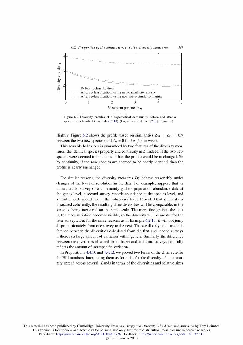
This material has been published by Cambridge University Press as Entropy and Diversity: The Axiomatic Approach by Tom Leinster.This version is free to view and download for personal use only. Not for re-distribution, re-sale or use in derivative works.
Paperback: https://www.cambridge.org/9781108965576. Hardback: https://www.cambridge.org/9781108832700.© Tom Leinster 2020
6.2 Properties of the similarity-sensitive diversity measures 189
1
2
3
4
0 1 2 3 4 5
Before reclassificationAfter reclassification, using naive similarity matrixAfter reclassification, using non-naive similarity matrix
Div
ersi
tyof
orde
rq
Viewpoint parameter, q
Figure 6.2 Diversity profiles of a hypothetical community before and after aspecies is reclassified (Example 6.2.10). (Figure adapted from [218], Figure 1.)
slightly. Figure 6.2 shows the profile based on similarities Z34 = Z43 = 0.9between the two new species (and Zi j = 0 for i , j otherwise).
This sensible behaviour is guaranteed by two features of the diversity mea-sures: the identical species property and continuity in Z. Indeed, if the two newspecies were deemed to be identical then the profile would be unchanged. Soby continuity, if the new species are deemed to be nearly identical then theprofile is nearly unchanged.
For similar reasons, the diversity measures DZq behave reasonably under
changes of the level of resolution in the data. For example, suppose that aninitial, crude, survey of a community gathers population abundance data atthe genus level, a second survey records abundance at the species level, anda third records abundance at the subspecies level. Provided that similarity ismeasured coherently, the resulting three diversities will be comparable, in thesense of being measured on the same scale. The more fine-grained the datais, the more variation becomes visible, so the diversity will be greater for thelater surveys. But for the same reasons as in Example 6.2.10, it will not jumpdisproportionately from one survey to the next. There will only be a large dif-ference between the diversities calculated from the first and second surveysif there is a large amount of variation within genera. Similarly, the differencebetween the diversities obtained from the second and third surveys faithfullyreflects the amount of intraspecific variation.
In Propositions 4.4.10 and 4.4.12, we proved two forms of the chain rule forthe Hill numbers, interpreting them as formulas for the diversity of a commu-nity spread across several islands in terms of the diversities and relative sizes

This material has been published by Cambridge University Press as Entropy and Diversity: The Axiomatic Approach by Tom Leinster.This version is free to view and download for personal use only. Not for re-distribution, re-sale or use in derivative works.
Paperback: https://www.cambridge.org/9781108965576. Hardback: https://www.cambridge.org/9781108832700.© Tom Leinster 2020
190 Species similarity and magnitude
of those islands. The islands were assumed to have no species in common. Wenow derive two forms of the chain rule for the more general similarity-sensitivediversity measures DZ
q (p), under the stronger assumption that the species ondifferent islands are not only distinct, but also completely dissimilar.
Thus, consider n island communities with relative abundance distributionsp1 ∈ ∆k1 , . . . ,pn ∈ ∆kn , similarity matrices Z1, . . . ,Zn, and relative sizesw1, . . . ,wn (in the sense of Example 2.1.6). The species distribution of thewhole group is, then,
w (p1, . . . ,pn) ∈ ∆k,
where k = k1 + · · · + kn. Assuming that the species on different islands arecompletely dissimilar, the k × k similarity matrix Z for the whole group is theblock sum
Z = Z1 ⊕ · · · ⊕ Zn =
Z1 0 · · · 0
0 Z2 . . ....
.... . .
. . . 00 · · · 0 Zn
.
So, the diversity of the whole is
DZq(w (p1, . . . ,pn)
),
and our task is to express this in terms of the islands’ diversities DZi
q (pi) andtheir relative sizes wi.
Proposition 6.2.11 (Chain rule) Let q ∈ [0,∞] and n, k1, . . . , kn ≥ 1. Foreach i ∈ 1, . . . , n, let Zi be a ki × ki similarity matrix and let pi ∈ ∆ki ; also, letw ∈ ∆n. Write Z = Z1 ⊕ · · · ⊕ Zn and di = DZi
q (pi).
i. We have
DZq(w (p1, . . . ,pn)
)= M1−q(w,d/w)
=
(∑
wqi d1−q
i)1/(1−q) if q , 1,∞,∏
(di/wi)wi if q = 1,
min di/wi if q = ∞,
where d/w = (d1/w1, . . . , dn/wn) and the sum, product, and minimum areover all i ∈ supp(w).
ii. For q < ∞,
DZq(w (p1, . . . ,pn)
)= Dq(w) · M1−q(w(q),d),
where w(q) is the escort distribution defined after Proposition 4.4.10.

This material has been published by Cambridge University Press as Entropy and Diversity: The Axiomatic Approach by Tom Leinster.This version is free to view and download for personal use only. Not for re-distribution, re-sale or use in derivative works.
Paperback: https://www.cambridge.org/9781108965576. Hardback: https://www.cambridge.org/9781108832700.© Tom Leinster 2020
6.2 Properties of the similarity-sensitive diversity measures 191
Proof For (i), an elementary calculation shows that
Z(w (p1, . . . ,pn)
)= w1(Z1p1) ⊕ · · · ⊕ wn(Znpn).
Hence, using the chain rule for the power means and then the homogeneity ofthe power means,
DZq(w (p1, . . . ,pn)
)= M1−q
(w (p1, . . . ,pn),
1w1(Z1p1)
⊕ · · · ⊕1
wn(Znpn)
)= M1−q
(w,
(M1−q
(p1,
1w1(Z1p1)
), . . . ,M1−q
(pn,
1wn(Znpn)
)))= M1−q
(w,
(d1
w1, . . . ,
dn
wn
)).
This proves the first equality in (i), and the second follows from the explicitformulas for the power means. Lemma 4.4.11 then gives (ii).
In particular, the diversity of the overall community depends only on thesizes and diversities of the islands:
Corollary 6.2.12 (Modularity) In the situation of Proposition 6.2.11, the to-tal diversity DZ
q(w (p1, . . . ,pn)
)depends only on q, w, and DZ
q (p1), . . . ,DZ
q (pn).
A further consequence of the chain rule is also important. Suppose that theislands all have the same size and the same diversity, d. (For example, theislands will have the same diversity if they all have the same species dis-tributions, but on disjoint sets of species; or formally, if k1 = · · · = kn andp1 = · · · = pn.) Then in the notation of Proposition 6.2.11,
d/w =(d/(1/n), . . . , d/(1/n)
)= (nd, . . . , nd),
so
DZq(w (p1, . . . ,pn)
)= nd.
In other words, the diversity of a group of n islands, each having diversity d,is nd. This is the replication principle for the similarity-sensitive measuresDZ
q . It generalizes the replication principle for the Hill numbers, noted at theend of Section 4.4. The fact that our diversity measures satisfy it means thatthey do not suffer from the problems described in the oil company example(Example 2.4.11).
Since the diversity DZq , Renyi entropies HZ
q , and q-logarithmic entropies S Zq
are all related to one another by invertible transformations, the chain rule for

This material has been published by Cambridge University Press as Entropy and Diversity: The Axiomatic Approach by Tom Leinster.This version is free to view and download for personal use only. Not for re-distribution, re-sale or use in derivative works.
Paperback: https://www.cambridge.org/9781108965576. Hardback: https://www.cambridge.org/9781108832700.© Tom Leinster 2020
192 Species similarity and magnitude
DZq can be translated into chain rules for HZ
q and S Zq . In the case of S Z
q , it takesa simple form, generalizing the chain rule for q-logarithmic entropy (equa-tion (4.2)):
Proposition 6.2.13 (Chain rule) Let q ∈ [0,∞). For w, pi, Zi and Z as inProposition 6.2.11,
S Zq(w (p1, . . . ,pn)
)= S q(w) +
∑i∈supp(w)
wqi · S
Zi
q (pi).
Proof Proposition 6.2.11(i) gives
lnq(DZ
q(w (p1, . . . ,pn)
))= lnq
(M1−q(w,d/w)
).
By definition of S Zq (equation (6.4)) and Lemma 4.2.29, an equivalent state-
ment is that
S Zq(w (p1, . . . ,pn)
)=
∑i∈supp(w)
wi lnqdi
wi.
But writing di/wi = (1/wi)di and applying the formula (1.18) for the q-logarithm of a product, the right-hand side is∑
i∈supp(w)
wi
(lnq
1wi
+
(1wi
)1−q
lnq di
)=
∑i∈supp(w)
wi lnq1wi
+∑
i∈supp(w)
wqi lnq di
= S q(w) +∑
i∈supp(w)
wqi · S
Zq (pi).
6.3 Maximizing diversity
Consider a community made up of organisms drawn from a fixed list ofspecies, whose similarities to one another are known. Suppose that we cancontrol the abundances of the species within the community. How should wechoose those abundances in order to maximize the diversity, and what is themaximum diversity achievable?
In mathematical terms, fix an n × n similarity matrix Z. The fundamentalquestions are these:
• Which distributions p maximize the diversity DZq (p) of order q?
• What is the value of the maximum diversity, supp∈∆nDZ
q (p)?

This material has been published by Cambridge University Press as Entropy and Diversity: The Axiomatic Approach by Tom Leinster.This version is free to view and download for personal use only. Not for re-distribution, re-sale or use in derivative works.
Paperback: https://www.cambridge.org/9781108965576. Hardback: https://www.cambridge.org/9781108832700.© Tom Leinster 2020
6.3 Maximizing diversity 193
In principle, the answers to both questions depend on q. After all, we haveseen that when comparing two abundance distributions, different values of qmay produce different judgements on which of the distributions is more di-verse (as in Examples 4.3.9 and 6.1.8). For instance, there seems no reason tosuppose that a distribution maximizing diversity of order 1 will also maximizediversity of order 2. Similarly, we have seen nothing to suggest that the maxi-mum diversity supp DZ
1 (p) of order 1 should be equal to the maximum diversityof order 2.
However, it is a theorem that as long as Z is symmetric, the answers toboth questions are indeed independent of q. That is, every symmetric similaritymatrix has an unambiguous maximum diversity, and there is a distribution pthat maximizes DZ
q (p) for all q simultaneously.This result was first stated and proved by Leinster [209]. An improved proof
and further results were given in a paper of Leinster and Meckes [219], fromwhich much of this section is adapted. We omit most proofs, referring to [219].
Before stating the theorem, let us explore the maximum diversity probleminformally.
Examples 6.3.1 If there is only one species (n = 1) then the problem is trivial.If there are two then, assuming that Z is symmetric, their roles are interchange-able, so the distribution that maximizes diversity will clearly be (1/2, 1/2).
Now consider a three-species pond community consisting of two highly sim-ilar species of frog and one species of newt. If we ignore the similarity betweenthe species of frog and give the three species equal status, then the maximiz-ing distribution should be uniform: (1/3, 1/3, 1/3). But intuitively, this is notthe distribution that maximizes diversity, since it is 2/3 frog and 1/3 newt. Atthe other extreme, if we treat the two frog species as identical, then diversityis maximized when there are equal quantities of frogs and newts (as in thetwo-species example); so, the distribution (1/4, 1/4, 1/2) should maximize di-versity. In reality, with a reasonable measure of similarities between species,the distribution that maximizes diversity should be somewhere between thesetwo extremes. We will see in Example 6.3.16 that this is indeed the case.
For the rest of this section, fix an integer n ≥ 1 and an n × n symmetricsimilarity matrix Z. The symmetry hypothesis matters, as we will see in Ex-ample 6.3.17.
Theorem 6.3.2 (Maximum diversity) i. There exists a probability distribu-tion on 1, . . . , n that maximizes DZ
q for all q ∈ [0,∞] simultaneously.ii. The maximum diversity supp∈∆n
DZq (p) is independent of q ∈ [0,∞].
Proof This is Theorem 1 of [219].
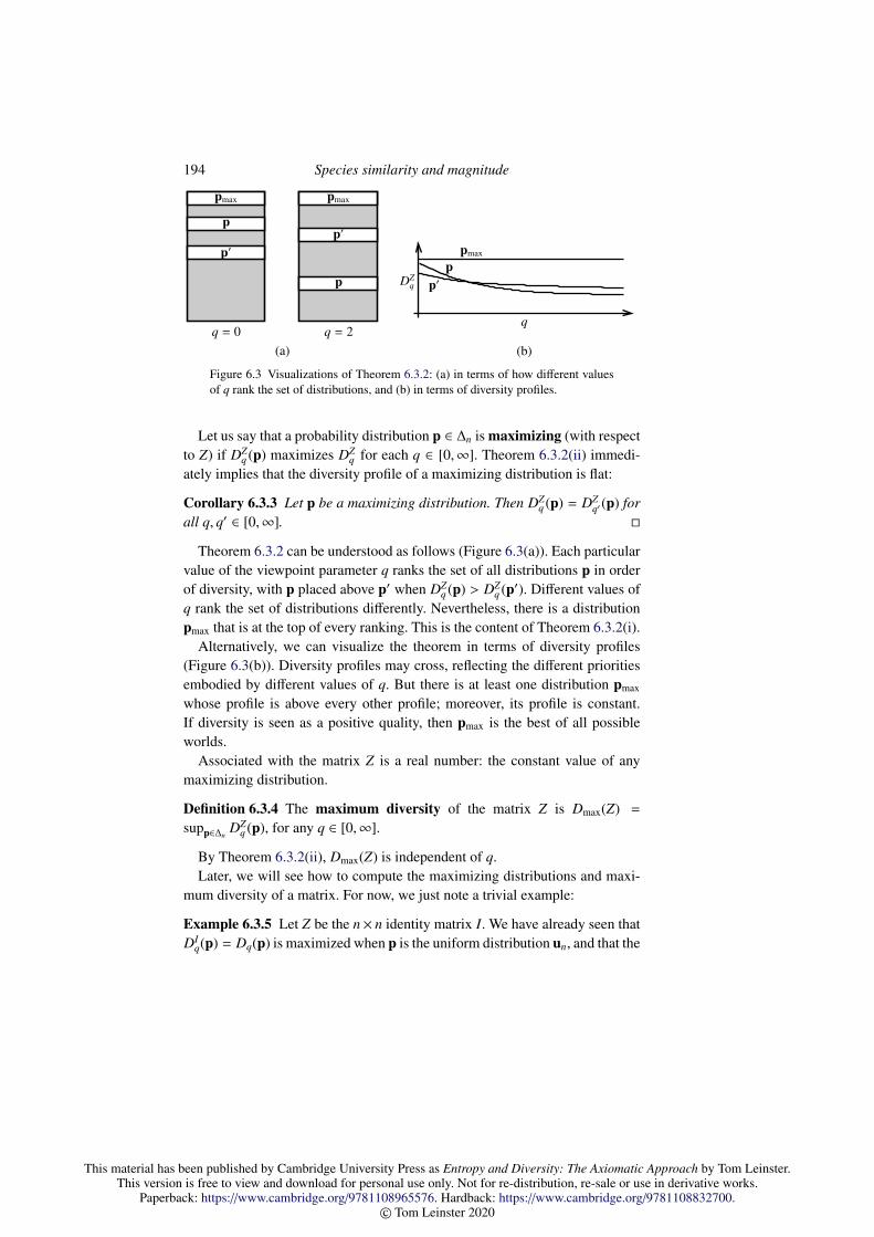
This material has been published by Cambridge University Press as Entropy and Diversity: The Axiomatic Approach by Tom Leinster.This version is free to view and download for personal use only. Not for re-distribution, re-sale or use in derivative works.
Paperback: https://www.cambridge.org/9781108965576. Hardback: https://www.cambridge.org/9781108832700.© Tom Leinster 2020
194 Species similarity and magnitude
(a)q = 0
pmax
p
p′
q = 2
pmax
p′
p
(b)
DZq
q
pp′
pmax
Figure 6.3 Visualizations of Theorem 6.3.2: (a) in terms of how different valuesof q rank the set of distributions, and (b) in terms of diversity profiles.
Let us say that a probability distribution p ∈ ∆n is maximizing (with respectto Z) if DZ
q (p) maximizes DZq for each q ∈ [0,∞]. Theorem 6.3.2(ii) immedi-
ately implies that the diversity profile of a maximizing distribution is flat:
Corollary 6.3.3 Let p be a maximizing distribution. Then DZq (p) = DZ
q′ (p) forall q, q′ ∈ [0,∞].
Theorem 6.3.2 can be understood as follows (Figure 6.3(a)). Each particularvalue of the viewpoint parameter q ranks the set of all distributions p in orderof diversity, with p placed above p′ when DZ
q (p) > DZq (p′). Different values of
q rank the set of distributions differently. Nevertheless, there is a distributionpmax that is at the top of every ranking. This is the content of Theorem 6.3.2(i).
Alternatively, we can visualize the theorem in terms of diversity profiles(Figure 6.3(b)). Diversity profiles may cross, reflecting the different prioritiesembodied by different values of q. But there is at least one distribution pmax
whose profile is above every other profile; moreover, its profile is constant.If diversity is seen as a positive quality, then pmax is the best of all possibleworlds.
Associated with the matrix Z is a real number: the constant value of anymaximizing distribution.
Definition 6.3.4 The maximum diversity of the matrix Z is Dmax(Z) =
supp∈∆nDZ
q (p), for any q ∈ [0,∞].
By Theorem 6.3.2(ii), Dmax(Z) is independent of q.Later, we will see how to compute the maximizing distributions and maxi-
mum diversity of a matrix. For now, we just note a trivial example:
Example 6.3.5 Let Z be the n× n identity matrix I. We have already seen thatDI
q(p) = Dq(p) is maximized when p is the uniform distribution un, and that the
This material has been published by Cambridge University Press as Entropy and Diversity: The Axiomatic Approach by Tom Leinster.This version is free to view and download for personal use only. Not for re-distribution, re-sale or use in derivative works.
Paperback: https://www.cambridge.org/9781108965576. Hardback: https://www.cambridge.org/9781108832700.© Tom Leinster 2020
6.3 Maximizing diversity 195
maximum value is n (Lemma 4.4.3(ii)). It is a special case of Theorem 6.3.2(ii)that this maximum value, n, is independent of q. In the notation just introduced,Dmax(I) = n.
If a distribution p maximizes diversity of order 2, must it also maximizediversity of orders 1 and∞, for instance? The answer turns out to be yes:
Corollary 6.3.6 Let p ∈ ∆n. If p maximizes DZq for some q ∈ (0,∞] then p
maximizes DZq for all q ∈ [0,∞].
Proof This is Corollary 2 of [219].
The significance of this result is that if we wish to find a distribution thatmaximizes diversity of all orders q, all we need to do is to find one that maxi-mizes diversity of whichever nonzero order is most convenient.
The hypothesis that q > 0 cannot be dropped from Corollary 6.3.6. Indeed,take Z = I. Then DI
0(p) is species richness (the cardinality of supp(p)), whichis maximized by any distribution p of full support. On the other hand, whenq > 0, the diversity DI
q(p) = Dq(p) is maximized only when p is uniform(Lemma 4.4.3(ii)).
Remark 6.3.7 Since the similarity-sensitive Renyi entropy HZq and similarity-
sensitive q-logarithmic entropy S Zq are increasing transformations of DZ
q , thesame distributions that maximize DZ
q for all q also maximize HZq and S Z
q for allq. And since HZ
q = log DZq , the maximum similarity-sensitive Renyi entropy,
supp HZq (p), is also independent of q: it is simply log Dmax(Z).
In contrast, the maximum similarity-sensitive q-logarithmic entropy,supp S Z
q (p), is not independent of q. It is lnq Dmax(Z), which varies with q.This is one advantage of the Renyi entropy (and its exponential) over the q-logarithmic entropy.
Theorem 6.3.2 guarantees the existence of a maximizing distribution pmax,but does not tell us how to find one. It also states that DZ
q (pmax) is independentof q, but does not tell us its value. Our next theorem repairs both omissions. Tostate it, we need some definitions.
Definition 6.3.8 A weighting on a matrix M is a column vector w such that
Mw =
1...
1
.Lemma 6.3.9 Let M be a matrix. Suppose that M and its transpose MT eachhave at least one weighting. Then
∑i wi is independent of the choice of weight-
ing w on M.
This material has been published by Cambridge University Press as Entropy and Diversity: The Axiomatic Approach by Tom Leinster.This version is free to view and download for personal use only. Not for re-distribution, re-sale or use in derivative works.
Paperback: https://www.cambridge.org/9781108965576. Hardback: https://www.cambridge.org/9781108832700.© Tom Leinster 2020
196 Species similarity and magnitude
Proof Let w and w′ be weightings on M. Choose a weighting v on MT. Then
∑i
wi = (1 · · · 1)w =(MTv
)Tw = vTMw = vT
1...
1
=∑
j
v j.
Similarly,∑
i w′i =∑
j v j. Hence∑
i wi =∑
i w′i .
Definition 6.3.10 Let M be a matrix such that both M and MT have at leastone weighting. Its magnitude |M| is
∑i wi, where w is any weighting on M.
By Lemma 6.3.9, the magnitude is independent of the choice of weighting.
Remarks 6.3.11 i. When M is symmetric (the case of interest here), |M| isdefined as long as M has at least one weighting.
ii. When M is invertible, M has exactly one weighting. Its entries are the row-sums of M−1. Thus, |M| is the sum of all the entries of M−1.
Definition 6.3.12 A vector v = (vi) over R is nonnegative if vi ≥ 0 for all i,and positive if vi > 0 for all i.
For a nonempty subset B ⊆ 1, . . . , n, let ZB denote the submatrix (Zi j)i, j∈B
of Z. This is also a symmetric similarity matrix. Suppose that we have a non-negative weighting w on ZB. Then w , 0, so
∑j∈B w j , 0. We can therefore
define a probability distribution w ∈ ∆n by normalizing and extending by 0:
wi =
wi/|ZB| if i ∈ B,
0 otherwise
(i ∈ 1, . . . , n).
Theorem 6.3.13 (Computation of maximum diversity) i. The maximumdiversity of Z is given by
Dmax(Z) = maxB|ZB|, (6.11)
where the maximum is over all nonempty B ⊆ 1, . . . , n such that ZB admitsa nonnegative weighting.
ii. The set of maximizing distributions is⋃B
w : nonnegative weightings w on B,
where the union is over all B attaining the maximum in (6.11).
Proof This is Theorem 2 of [219].

This material has been published by Cambridge University Press as Entropy and Diversity: The Axiomatic Approach by Tom Leinster.This version is free to view and download for personal use only. Not for re-distribution, re-sale or use in derivative works.
Paperback: https://www.cambridge.org/9781108965576. Hardback: https://www.cambridge.org/9781108832700.© Tom Leinster 2020
6.3 Maximizing diversity 197
Remark 6.3.14 Let B ⊆ 1, . . . , n be a subset attaining the maximumin (6.11), and let w be a nonnegative weighting on ZB, so that w ∈ ∆n is amaximizing distribution. A short calculation shows that
(Zw)i =1|ZB|
for all i ∈ B. In particular, (Zw)i is constant over i ∈ B. This can be understoodas follows. For the Hill numbers (the case Z = I), the maximizing distributiontakes the relative abundances pi to be the same for all species i. This is nolonger true when inter-species similarities are taken into account. Instead, themaximizing distributions have the property that the ordinariness (Zp)i is thesame for all species i that are present.
Determining which species are present in a maximizing distribution is notstraightforward. In particular, maximizing distributions do not always have fullsupport, a phenomenon discussed at the end of this section.
Theorem 6.3.13 provides a finite-time algorithm for computing the maxi-mizing diversity of Z, as well as all its maximizing distributions, as follows.
For each of the 2n−1 nonempty subsets B of 1, . . . , n, perform some simplelinear algebra to find the space of nonnegative weightings on ZB. If this spaceis nonempty, call B feasible and record the magnitude |ZB|. Then Dmax(Z) isthe maximum of all the recorded magnitudes. For each feasible B such that|ZB| = Dmax(Z), and each nonnegative weighting w on ZB, the distribution w ismaximizing. This generates all of the maximizing distributions.
This algorithm takes exponentially many steps in n, and Remark 6.3.24 pro-vides strong evidence that no algorithm can compute maximum diversity inpolynomial time. But the situation is not as hopeless as it might appear, fortwo reasons.
First, each step of the algorithm is fast, consisting as it does of solving asystem of linear equations. For instance, using a standard laptop and a standardcomputer algebra package, with no attempt at optimization, the maximizingdistributions of 25× 25 matrices were computed in a few seconds. Second, forcertain classes of matrices Z, the computing time can be reduced dramatically,as we will see.
We first consider some examples, starting with the most simple cases.
Example 6.3.15 Take a 2 × 2 similarity matrix
Z =
(1 zz 1
),
where 0 ≤ z < 1. Let us run the algorithm just described.

This material has been published by Cambridge University Press as Entropy and Diversity: The Axiomatic Approach by Tom Leinster.This version is free to view and download for personal use only. Not for re-distribution, re-sale or use in derivative works.
Paperback: https://www.cambridge.org/9781108965576. Hardback: https://www.cambridge.org/9781108832700.© Tom Leinster 2020
198 Species similarity and magnitude
Z =
1 0.9 0.40.9 1 0.40.4 0.4 1
newtfrog species A
frog species B0.9
0.4
0.4
Figure 6.4 Hypothetical three-species system. Distances between species indicatedegrees of dissimilarity between them (not to scale).
• First we determine for which nonempty B ⊆ 1, . . . , n the submatrix ZB hasa nonnegative weighting, and record the magnitudes of those that do.
When B = 1, the submatrix ZB is (1); this has a unique nonnegativeweighting w = (1), so |ZB| = 1. The same is true for B = 2. When B =
1, 2, we have ZB = Z, which has a unique nonnegative weighting
w =1
1 + z
(11
)(6.12)
and magnitude |ZB| = 2/(1 + z).• The maximum diversity of Z is given by
Dmax(Z) = max
1, 1,2
1 + z
,
and 2/(1 + z) > 1, so Dmax(Z) = 2/(1 + z). The unique maximizing dis-tribution is the normalization of the weighting (6.12), which is the uniformdistribution u2.
That the maximizing distribution is uniform conforms to the intuitive expec-tation of Example 6.3.1. The computed value of Dmax(Z) also conforms to theexpectation that the maximum diversity should be a decreasing function of thesimilarity between the species.
Example 6.3.16 Now consider the three-species pond community of Exam-ple 6.3.1, with similarities as shown in Figure 6.4. Implementing the algorithmor using Proposition 6.3.25 below reveals that the unique maximizing distribu-tion is (0.478, 0.261, 0.261) (to 3 decimal places). This confirms the intuitiveguess of Example 6.3.1.
One of our standing hypotheses on Z is symmetry. Without it, the main the-orem fails in every respect:
Example 6.3.17 Let Z =(
1 1/20 1
), which is a similarity matrix but not sym-
metric. Consider a distribution p = (p1, p2) ∈ ∆2. If p is (1, 0) or (0, 1) then

This material has been published by Cambridge University Press as Entropy and Diversity: The Axiomatic Approach by Tom Leinster.This version is free to view and download for personal use only. Not for re-distribution, re-sale or use in derivative works.
Paperback: https://www.cambridge.org/9781108965576. Hardback: https://www.cambridge.org/9781108832700.© Tom Leinster 2020
6.3 Maximizing diversity 199
DZq (p) = 1 for all q. Otherwise,
DZ0 (p) = 3 −
21 + p1
, (6.13)
DZ2 (p) =
23(p1 − 1/2)2 + 5/4
, (6.14)
DZ∞(p) =
1
1−p1if p1 ≤ 1/3,
21+p1
if p1 ≥ 1/3.(6.15)
It follows that supp∈∆2DZ
0 (p) = 2. However, no distribution maximizes DZ0 ; we
have DZ0 (p) → 2 as p → (1, 0), but DZ
0 (1, 0) = 1. Equations (6.14) and (6.15)imply that
supp∈∆2
DZ2 (p) = 1.6, sup
p∈∆2
DZ∞(p) = 1.5,
with unique maximizing distributions (1/2, 1/2) and (1/3, 2/3) respectively.Thus, when Z is not symmetric, the main theorem fails comprehensively:
the supremum supp∈∆nDZ
0 (p) may not be attained; there may be no distributionmaximizing supp∈∆n
DZq (p) for all q simultaneously; and that supremum may
vary with q.
Perhaps surprisingly, nonsymmetric similarity matrices Z do have practicaluses. For example, it is shown in Proposition A7 of the appendix to Leinsterand Cobbold [218] that the mean phylogenetic diversity measures of Chao,Chiu and Jost [65] are a special case of the measures DZ
q (p), obtained by tak-ing a particular Z constructed from the phylogenetic tree concerned. This Zis usually nonsymmetric, reflecting the asymmetry of evolutionary time. Moregenerally, the case for dropping the symmetry axiom for metric spaces wasmade by Lawvere (p. 138–139 of [202]), and Gromov has argued that sym-metry ‘unpleasantly limits many applications’ (p. xv of [129]). So, the factthat the maximum diversity theorem fails for nonsymmetric Z is an importantrestriction.
Now consider finite, undirected graphs with no multiple edges (henceforth,graphs for short). As in Example 6.1.4, any such graph corresponds to a sym-metric similarity matrix. What, then, is the maximum diversity of the adjacencymatrix of a graph?
The answer requires some terminology. Recall that vertices x and y of agraph are said to be adjacent, written as x ∼ y, if there is an edge betweenthem. (In particular, every vertex of a reflexive graph is adjacent to itself.) Aset of vertices is independent if no two distinct vertices are adjacent. The
This material has been published by Cambridge University Press as Entropy and Diversity: The Axiomatic Approach by Tom Leinster.This version is free to view and download for personal use only. Not for re-distribution, re-sale or use in derivative works.
Paperback: https://www.cambridge.org/9781108965576. Hardback: https://www.cambridge.org/9781108832700.© Tom Leinster 2020
200 Species similarity and magnitude
independence number α(G) of a graph G is the number of vertices in anindependent set of greatest cardinality.
Proposition 6.3.18 Let G be a reflexive graph with adjacency matrix Z. Thenthe maximum diversity Dmax(Z) is equal to the independence number α(G).
Proof We will maximize the diversity of order ∞. For any probability distri-bution p on the vertex-set 1, . . . , n,
DZ∞(p) = 1
/max
i∈supp(p)
∑j : i∼ j
p j. (6.16)
First we show that Dmax(Z) ≥ α(G). Choose an independent set B of cardi-nality α(G), and define p ∈ ∆n by
pi =
1/α(G) if i ∈ B,
0 otherwise.
For each i ∈ supp(p) = B, the sum on the right-hand side of equation (6.16) is1/α(G). Hence DZ
∞(p) = α(G), giving Dmax(Z) ≥ α(G).Now we show that Dmax(Z) ≤ α(G). By equation (6.16), an equivalent state-
ment is that for each p ∈ ∆n, there is some i ∈ supp(p) such that∑j : i∼ j
p j ≥1
α(G). (6.17)
Let p ∈ ∆n. Choose an independent set B ⊆ supp(p) with maximal cardinalityamong all independent subsets of supp(p). Then every vertex in supp(p) isadjacent to at least one vertex in B, otherwise we could adjoin it to B to makea larger independent subset. This gives the inequality∑
i∈B
∑j : i∼ j
p j =∑i∈B
∑j∈supp(p) : i∼ j
p j ≥∑
j∈supp(p)
p j = 1.
So we can choose some i ∈ B such that∑
j : i∼ j p j ≥ 1/#B, where # denotes car-dinality. But #B ≤ α(G) since B is independent, so the desired inequality (6.17)follows.
Remark 6.3.19 The first part of the proof (together with Corollary 6.3.6)shows that a maximizing distribution on a reflexive graph can be constructedby taking the uniform distribution on some independent set of greatest cardi-nality, then extending by zero to the whole vertex-set. Except in the trivial caseof a graph with no edges between distinct vertices, this maximizing distributionnever has full support.

This material has been published by Cambridge University Press as Entropy and Diversity: The Axiomatic Approach by Tom Leinster.This version is free to view and download for personal use only. Not for re-distribution, re-sale or use in derivative works.
Paperback: https://www.cambridge.org/9781108965576. Hardback: https://www.cambridge.org/9781108832700.© Tom Leinster 2020
6.3 Maximizing diversity 201
Example 6.3.20 The reflexive graph G = •−•−• (loops not shown) has adja-
cency matrix Z =
(1 1 01 1 10 1 1
). The independence number of G is 2; this, then, is
the maximum diversity of Z. There is a unique independent set of cardinality2, and a unique maximizing distribution, (1/2, 0, 1/2).
Example 6.3.21 The reflexive graph •−•−•−• also has independence num-ber 2. There are three independent sets of maximal cardinality, so by Re-mark 6.3.19, there are at least three maximizing distributions,( 1
2 , 0,12 , 0
),
( 12 , 0, 0,
12),
(0, 1
2 , 0,12),
all with different supports. (The possibility of multiple maximizing distribu-tions was also observed in the case q = 2 by Pavoine and Bonsall [272].) Infact, there are further maximizing distributions not constructed in the proof ofProposition 6.3.18, namely,
( 12 , 0, t,
12 − t
)and
( 12 − t, t, 0, 1
2)
for all t ∈ (0, 12 ).
Example 6.3.22 Kolmogorov’s notion of the ε-entropy of a metric space [191]is approximately an instance of maximum diversity, assuming that one is inter-ested in its behaviour as ε→ 0 rather than for individual values of ε.
Let A be a finite metric space. Given ε > 0, the ε-covering number Nε(A)is the smallest number of closed ε-balls needed to cover A. But also associatedwith ε is the graph Gε(A) whose vertices are the points of A and with an edgebetween a and b whenever d(a, b) ≤ ε. Write Zε(A) for the adjacency matrixof Gε(A). From Proposition 6.3.18, it is not hard to deduce that
Nε(A) ≤ Dmax(Zε(A)) ≤ Nε/2(A)
(Example 11 of [219]).We have repeatedly seen that quantities called entropy tend to be the
logarithms of quantities called diversity. Kolmogorov’s ε-entropy of A islog Nε(A), and, by the inequalities above, is closely related to the logarithmof maximum diversity.
The moral of the proof of Proposition 6.3.18 is that by performing the simpletask of maximizing diversity of order∞, we automatically maximize diversityof all other orders. Here is an example of how this observation can be exploited.
Every graph G has a complement G, with the same vertex-set as G; twovertices are adjacent in G if and only if they are not adjacent in G. Thus, thecomplement of a reflexive graph is irreflexive (has no loops), and vice versa.A set B of vertices in an irreflexive graph X is a clique if all pairs of distinctelements of B are adjacent in X. The clique number ω(X) of X is the maximalcardinality of a clique in X. Thus, ω(X) = α
(X).

This material has been published by Cambridge University Press as Entropy and Diversity: The Axiomatic Approach by Tom Leinster.This version is free to view and download for personal use only. Not for re-distribution, re-sale or use in derivative works.
Paperback: https://www.cambridge.org/9781108965576. Hardback: https://www.cambridge.org/9781108832700.© Tom Leinster 2020
202 Species similarity and magnitude
We now recover a result of Berarducci, Majer and Novaga (Proposition 5.10of [35]).
Corollary 6.3.23 (Berarducci, Majer and Novaga) Let X be an irreflexivegraph. Then
supp
∑(i, j) : i∼ j
pi p j = 1 −1
ω(X),
where the supremum is over probability distributions p on the vertex-set of Xand the sum is over ordered pairs of adjacent vertices of X.
Proof Write 1, . . . , n for the vertex-set of X, and Z for the adjacency matrixof the reflexive graph X. Then for all p ∈ ∆n,
∑(i, j) : i∼ j in X
pi p j =
n∑i, j=1
pi p j −∑
(i, j) : i∼ j in X
pi p j
= 1 −n∑
i, j=1
piZi j p j
= 1 −1
DZ2 (p)
.
Hence by Proposition 6.3.18,
supp∈∆n
∑(i, j) : i∼ j in X
pi p j = 1 −1
Dmax(p)= 1 −
1
α(X) = 1 −
1ω(X)
.
It follows from this proof and Remark 6.3.19 that∑
(i, j) : i∼ j pi p j can be maxi-mized as follows: take the uniform distribution on some clique in X of maximalcardinality, then extend by zero to the whole vertex-set. This distribution max-imizes the probability that two vertices chosen at random are adjacent, as inExample 6.1.6(iv).
Remark 6.3.24 Proposition 6.3.18 implies that computationally, finding themaximum diversity of an arbitrary symmetric n × n similarity matrix is atleast as hard as finding the independence number of a reflexive graph withn vertices. This is a very well-studied problem, usually presented in its dualform (find the clique number of an irreflexive graph) and called the maximumclique problem [179]. It is NP-hard. Hence, assuming that P , NP, there isno polynomial-time algorithm for computing maximum diversity, nor even forcomputing the support of a maximizing distribution.

This material has been published by Cambridge University Press as Entropy and Diversity: The Axiomatic Approach by Tom Leinster.This version is free to view and download for personal use only. Not for re-distribution, re-sale or use in derivative works.
Paperback: https://www.cambridge.org/9781108965576. Hardback: https://www.cambridge.org/9781108832700.© Tom Leinster 2020
6.3 Maximizing diversity 203
We now return to general symmetric similarity matrices, addressing two re-maining questions: when are maximizing distributions unique, and when dothey have full support?
Recall that a real symmetric matrix Z is positive definite if xTZx > 0 for all0 , x ∈ Rn, and positive semidefinite if xTZx ≥ 0 for all x ∈ Rn. Equivalently,Z is positive definite if all its eigenvalues are positive, and positive semidefiniteif they are all nonnegative. A positive definite matrix is invertible and thereforehas a unique weighting.
Proposition 6.3.25 i. If Z is positive semidefinite and has a nonnegativeweighting w, then Dmax(Z) = |Z| and w/|Z| is a maximizing distribution.
ii. If Z is positive definite and its unique weighting w is positive then w/|Z| isthe unique maximizing distribution.
Proof This is Proposition 3 of [219].
In particular, if |Z| is positive semidefinite and has a nonnegative weighting,then computing its maximum diversity is trivial.
When Z is positive definite and its unique weighting is positive, its uniquemaximizing distribution eliminates no species. Here are two classes of suchmatrices Z.
Example 6.3.26 Call Z ultrametric if Zik ≥ minZi j,Z jk for all i, j, k andZii > Z jk for all i, j, k with j , k. For instance, the matrix Z =
(e−d(i, j)) of
any ultrametric space is ultrametric; see Example 6.1.3. If Z is ultrametric thenZ is positive definite with positive weighting, by Proposition 2.4.18 of Lein-ster [214].
(The positive definiteness of ultrametric matrices was also proved, earlier, byVarga and Nabben [340], and a different proof still was given in Theorem 3.6of Meckes [248]. An earlier, indirect proof of the positivity of the weightingcan be found in Pavoine, Ollier and Pontier [273].)
Such matrices arise in practice. For instance, Z is ultrametric if it is definedfrom a phylogenetic or taxonomic tree as in Examples 6.1.1(iii) and (iv).
Example 6.3.27 The identity matrix Z = I is certainly positive definite withpositive weighting. By topological arguments, there is a neighbourhood U of Iin the space of symmetric matrices such that every matrix in U also has theseproperties. (See the proofs of Propositions 2.2.6 and 2.4.6 of Leinster [214].)
Quantitative versions of this result are also available. For instance, supposethat Zii = 1 for all i, j and that Z is strictly diagonally dominant, that is,Zii >
∑j,i Zi j for all i. Then Z is positive definite with positive weighting
(Proposition 4 of Leinster and Meckes [219]).

This material has been published by Cambridge University Press as Entropy and Diversity: The Axiomatic Approach by Tom Leinster.This version is free to view and download for personal use only. Not for re-distribution, re-sale or use in derivative works.
Paperback: https://www.cambridge.org/9781108965576. Hardback: https://www.cambridge.org/9781108832700.© Tom Leinster 2020
204 Species similarity and magnitude
oakpine
Figure 6.5 Hypothetical community consisting of one species of oak () and tenspecies of pine (•), to which one further species of pine is then added (). Dis-tances between species indicate degrees of dissimilarity (not to scale).
In summary, if our similarity matrix Z is ultrametric, or if it is close to thematrix I that encodes the naive model, then it enjoys many special properties:the maximum diversity is equal to the magnitude, there is a unique maximizingdistribution, the maximizing distribution has full support, and both the maxi-mizing distribution and the maximum diversity can be computed in polynomialtime.
We saw in Examples 6.3.20 and 6.3.21 that for some similarity matricesZ, no maximizing distribution has full support. Mathematically, this simplymeans that maximizing distributions sometimes lie on the boundary of ∆n.But ecologically, it may sound shocking: is it reasonable that diversity can beincreased by eliminating some species?
We argue that it is. For example, consider a forest consisting of one speciesof oak and ten species of pine, with all species equally abundant. Suppose thatan eleventh species of pine is added, with the same abundance as all the exist-ing species (Figure 6.5). This makes the forest even more heavily dominated bypine than it was before, so it is intuitively reasonable that the diversity shoulddecrease. But now running time backwards, the conclusion is that if we startwith a forest containing the oak and all eleven pine species, then eliminatingthe eleventh should increase the diversity.
To clarify further, recall that diversity is defined in terms of the relativeabundances only. Thus, eliminating the ith species causes not only a decrease inpi, but also an increase in the other relative abundances p j. If the ith species isparticularly ordinary within the community (like the eleventh species of pine),then eliminating it increases the relative abundances of less ordinary species,resulting in a community that is more diverse.
The instinct that maximizing diversity should not eliminate any species isbased on the assumption that the distinction between species is of high value.(After all, if two species were very nearly identical – or in the extreme, actuallyidentical – then losing one would be of little importance.) If one wishes to makethat assumption, one must build it into the model. This is done by choosing a

This material has been published by Cambridge University Press as Entropy and Diversity: The Axiomatic Approach by Tom Leinster.This version is free to view and download for personal use only. Not for re-distribution, re-sale or use in derivative works.
Paperback: https://www.cambridge.org/9781108965576. Hardback: https://www.cambridge.org/9781108832700.© Tom Leinster 2020
6.3 Maximizing diversity 205
similarity matrix Z with a low similarity coefficient Zi j for each i , j. Thus,Z is close to the identity matrix I (assuming that similarity is measured on ascale of 0 to 1). Example 6.3.27 guarantees that in this case, there is a uniquemaximizing distribution and it does not, in fact, eliminate any species.
The fact that maximizing distributions can eliminate some species has previ-ously been discussed in the ecological literature in the case of Rao’s quadraticentropy (q = 2): see Izsak and Szeidl [150], Pavoine and Bonsall [272], andreferences therein. The same phenomenon was observed and explored by Shi-matani in genetics [309], again in the case q = 2.
We finish by stating necessary and sufficient conditions for a symmetric sim-ilarity matrix Z to admit at least one maximizing distribution of full support,so that diversity can be maximized without eliminating any species. We alsostate necessary and sufficient conditions for every maximizing distribution tohave full support. The latter conditions are genuinely more restrictive. For in-stance, if Z =
( 1 11 1
)then every distribution is maximizing, so some but not all
maximizing distributions have full support.
Proposition 6.3.28 The following are equivalent:
i. there exists a maximizing distribution for Z of full support;ii. Z is positive semidefinite and has at least one positive weighting.
Proof This is Proposition 5 of [219].
Proposition 6.3.29 The following are equivalent:
i. every maximizing distribution for Z has full support;ii. Z has exactly one maximizing distribution, which has full support;
iii. Z is positive definite with positive weighting;iv. Dmax(ZB) < Dmax(Z) for every nonempty proper subset B of 1, . . . , n.
Proof This is Proposition 6 of [219].
Let us put our results on maximum diversity into context. First, they belongto the huge body of work on maximum entropy. For example, among all prob-ability distributions on R with a given mean and variance, the one with themaximum entropy is the normal distribution [230, 29]. Given the fundamentalnature of the normal distribution, this fact alone would be motivation enoughto seek maximum entropy distributions in other settings (such as the one athand), quite apart from the importance of maximum entropy in thermodynam-ics, machine learning, and so on.
Second, the maximum diversity theorem (Theorem 6.3.2) is stated for prob-ability distributions on finite sets equipped with a similarity matrix, but it can

This material has been published by Cambridge University Press as Entropy and Diversity: The Axiomatic Approach by Tom Leinster.This version is free to view and download for personal use only. Not for re-distribution, re-sale or use in derivative works.
Paperback: https://www.cambridge.org/9781108965576. Hardback: https://www.cambridge.org/9781108832700.© Tom Leinster 2020
206 Species similarity and magnitude
be generalized to compact Hausdorff spaces A equipped with a suitable func-tion Z : A×A→ [0,∞) measuring similarity between points. This more generaltheorem was recently proved by Leinster and Roff [221], along with a versionof the computation theorem (Theorem 6.3.13). It encompasses both the finitecase and the case of a compact metric space with similarities Z(a, b) = e−d(a,b).
Third, maximum diversity is closely related to the emerging invariant knownas magnitude, as now described.
6.4 Introduction to magnitude
In the solution to the maximum diversity problem, a supporting role was playedby the notion of the magnitude of a matrix (Definition 6.3.10). Theorem 6.3.13implies that the maximum diversity of a symmetric similarity matrix Z is al-ways equal to the magnitude of one of its principal submatrices ZB, and Ex-amples 6.3.26 and 6.3.27 describe classes of matrix for which the maximumdiversity is actually equal to the magnitude.
The definition of magnitude was introduced without motivation, and mayappear to be nothing but a technicality. But in fact, magnitude is an answer tothe following very broad conceptual challenge.
For many types of objects in mathematics, there is a canonical notion ofsize. For example:
• Every set A (finite, say) has a cardinality |A|, which satisfies the inclusion-exclusion formula
|A ∪ B| = |A| + |B| − |A ∩ B|
(for subsets A and B of some larger set) and the multiplicativity formula
|A × B| = |A| · |B|.
• Every measurable subset A of Euclidean space has a volume Vol(A), whichsatisfies similar formulas:
Vol(A ∪ B) = Vol(A) + Vol(B) − Vol(A ∩ B),
Vol(A × B) = Vol(A) · Vol(B).
• Every sufficiently well-behaved topological space A has an Euler character-istic χ(A), which again satisfies
χ(A ∪ B) = χ(A) + χ(B) − χ(A ∩ B),
χ(A × B) = χ(A) · χ(B).

This material has been published by Cambridge University Press as Entropy and Diversity: The Axiomatic Approach by Tom Leinster.This version is free to view and download for personal use only. Not for re-distribution, re-sale or use in derivative works.
Paperback: https://www.cambridge.org/9781108965576. Hardback: https://www.cambridge.org/9781108832700.© Tom Leinster 2020
6.4 Introduction to magnitude 207
a1
a2
a3
a4a5
Figure 6.6 The objects and maps of a finite category (identity maps not shown).
(Here, inclusion-exclusion holds for subspaces A and B of some largerspace, under suitable hypotheses. Technically, it is best to work in thesetting of either cohomology with compact supports, as in Section 3.3 ofHatcher [138], or tame topology, as in Chapter 4 of van den Dries [338] orChapter 3 of Ghrist [114].) The insight that Euler characteristic is the topo-logical analogue of cardinality is principally due to Schanuel, who comparedEuler’s investigation of spaces of negative ‘cardinality’ (Euler characteris-tic) with Cantor’s investigation of sets of infinite cardinality:
Euler’s analysis, which demonstrated that in counting suitably ‘finite’spaces one can get well-defined negative integers, was a revolutionaryadvance in the idea of cardinal number – perhaps even more importantthan Cantor’s extension to infinite sets, if we judge by the number ofareas in mathematics where the impact is pervasive.
([301], Section 3).
The close resemblance between these invariants suggests a challenge: find ageneral notion of the size of a mathematical object, encompassing these threeinvariants and others. And this challenge has a solution: the magnitude of anenriched category.
Enriched categories are very general structures, and the theory of the magni-tude of an enriched category sweeps across many parts of mathematics, most ofthem very distant from diversity measurement. This section and the next painta broad-brush picture, omitting all details. General references for this materialare Leinster and Meckes [220] and Leinster [214].
We begin with ordinary categories. A finite category A consists of, first ofall, a finite directed multigraph, that is, a finite collection of objects a1, . . . , an
together with a finite set Hom(ai, a j) for each i and j, whose elements are tobe thought of as maps or arrows from ai to a j (Figure 6.6). It is also equippedwith an associative operation of composition of maps and an identity map oneach object. (See Mac Lane [234], for instance.)
Any finite category A gives rise to an n × n matrix ZA whose (i, j)-entry is

This material has been published by Cambridge University Press as Entropy and Diversity: The Axiomatic Approach by Tom Leinster.This version is free to view and download for personal use only. Not for re-distribution, re-sale or use in derivative works.
Paperback: https://www.cambridge.org/9781108965576. Hardback: https://www.cambridge.org/9781108832700.© Tom Leinster 2020
208 Species similarity and magnitude
|Hom(ai, a j)|, the number of maps from ai to a j. The magnitude |A| ∈ Q of thecategory A is defined to be the magnitude |ZA| of the matrix ZA, if it exists.
Here we have used the notation | · | for two purposes: first for the cardinalityof a finite set, then for the magnitude of a category. This is deliberate. In bothcases, | · | is a measure of the size of the structure concerned.
For example, if A has no maps except for identities then ZA is the n × nidentity matrix, so the magnitude |A| is the cardinality n of its set of objects.Less trivially, any (small) category A has a classifying space BA (also called itsnerve or geometric realization), which is a topological space constructed fromA by starting with one 0-simplex for each object of A, then pasting in one 1-simplex for each map in A, one 2-simplex for each commutative triangle in A,and so on (Segal [305]). It is a theorem that
|A| = χ(BA), (6.18)
under finiteness conditions to ensure that the Euler characteristic of BA is well-defined (Proposition 2.11 of Leinster [208]). So, the situation is similar togroup homology: the homology of a group G can be defined either througha direct algebraic formula (as for |A|) or as the homology of its classifyingspace (as for χ(BA)), and it is a theorem that the two are equal.
Example 6.4.1 Let A = (•⇒ •) (identity maps not shown). Then
ZA =
(1 20 1
),
giving
Z−1A =
(1 −20 1
)and so
|A| = |ZA| = 1 + (−2) + 0 + 1 = 0.
On the other hand, BA = S 1, so χ(BA) = 0, confirming equation (6.18).
Equation (6.18) shows how, under hypotheses, magnitude for categories canbe derived from Euler characteristic for topological spaces. In the other di-rection, we can derive topological Euler characteristic from categorical mag-nitude. Let M be a finitely triangulated manifold. Then associated with thetriangulation, there is a category AM whose objects are the simplices s1, . . . , sn
of the triangulation, with one map si → s j whenever si ⊆ s j, and with no mapssi → s j otherwise. Then
χ(M) = |AM |

This material has been published by Cambridge University Press as Entropy and Diversity: The Axiomatic Approach by Tom Leinster.This version is free to view and download for personal use only. Not for re-distribution, re-sale or use in derivative works.
Paperback: https://www.cambridge.org/9781108965576. Hardback: https://www.cambridge.org/9781108832700.© Tom Leinster 2020
6.4 Introduction to magnitude 209
(Section 3.8 of Stanley [317] and Section 2 of Leinster [208]).The moral of the last two results is that topological Euler characteristic and
categorical magnitude each determine the other (under suitable hypotheses).Indeed, the magnitude of a category is often called its Euler characteristic;see, for instance, Leinster [208], Berger and Leinster [37], Fiore, Luck andSauer [103, 104], Noguchi [261, 262, 263], and Tanaka [320].
Further theorems connect the magnitude of a category to the Euler character-istic of an orbifold (Proposition 2.12 of [208]) and to the Baez–Dolan cardinal-ity of a groupoid (Example 2.7 of [208] and Section 3 of Baez and Dolan [23]),both of which are rational numbers, not usually integers. The notion of mag-nitude can also be seen as an extension of the theory of Mobius inversion forposets (most commonly associated with the name of Rota [298]), which itselfgeneralizes the classical Mobius function of number theory; see [208, 213] forexplanation.
The definition of the magnitude of a category involved |Hom(ai, a j)|, thecardinality of the set of maps from ai to a j. Thus, we used the notion of thecardinality of a finite set to define the magnitude of a finite category. We canenvisage that if Hom(ai, a j) were some other kind of structure with a preex-isting notion of size, a similar definition could be made. And indeed, this ideacan be implemented in the language of enriched categories, as follows.
A monoidal category is, loosely speaking, a category V equippedwith a product operation satisfying reasonable conditions. Section VII.1 ofMac Lane [234] gives the full definition, but the following examples will be allthat we need here.
Examples 6.4.2 Typical examples of monoidal categories are the category Setof sets with the cartesian product × and the category Vect of vector spaces withthe tensor product ⊗.
A less obvious example is the category whose objects are the elements ofthe interval [0,∞], with one map x → y whenever x ≥ y, and with no mapsx → y otherwise. Here we take + as the ‘product’ operation. (We could alsotake ordinary multiplication as the product, but it is + that will be of interesthere.)
Now fix a monoidal category V , with product denoted by ⊗. Loosely, acategory enriched in V , or V -category, A, consists of:
• a set a, b, . . . of objects of A;• for each pair (a, b) of objects of A, an object Hom(a, b) of V ;• for each triple (a, b, c) of objects of A, a map
Hom(a, b) ⊗ Hom(b, c)→ Hom(a, c) (6.19)

This material has been published by Cambridge University Press as Entropy and Diversity: The Axiomatic Approach by Tom Leinster.This version is free to view and download for personal use only. Not for re-distribution, re-sale or use in derivative works.
Paperback: https://www.cambridge.org/9781108965576. Hardback: https://www.cambridge.org/9781108832700.© Tom Leinster 2020
210 Species similarity and magnitude
in V (called composition in A),
subject to conditions. (For the full definition, see Section 1.2 of Kelly [182] orSection 6.2 of Borceux [45].)
Examples 6.4.3 The following examples of enriched categories are depictedin Figure 6.7.
i. A category enriched in (Set,×) is just an ordinary category. So, an enrichedcategory is not a category with special properties; it is something more gen-eral than a category.
ii. A category enriched in (Vect,⊗) is a linear category: a category equippedwith a vector space structure on each of the sets Hom(a, b), in such a waythat composition is bilinear.
iii. As first observed by Lawvere [202], any metric space A can be viewed asa category A enriched in ([0,∞],+): the objects of A are the points of A,while Hom(a, b) ∈ [0,∞] is the distance d(a, b), and the composition (6.19)is the triangle inequality
d(a, b) + d(b, c) ≥ d(a, c).
Thus, categories, linear categories and metric spaces are all instances ofa single general concept: enriched category. This enables constructions andinsights to be passed backwards and forwards between them, a strategy thatproves to have great power.
In particular, it is straightforward to generalize the definition of the mag-nitude of a finite category to finite enriched categories. Let V be a monoidalcategory equipped with a function | · | that assigns to each object X of V an el-ement |X| of some ring. This function | · | is to play the role of the cardinality ofa finite set, and we therefore impose the requirements that it is isomorphism-invariant and multiplicative:
X Y =⇒ |X| = |Y |, |X ⊗ Y | = |X| · |Y |.
(Section 1.3 of Leinster [214] gives details.) Then any V -category A withfinitely many objects, a1, . . . , an, gives rise to a matrix
ZA =(|Hom(ai, a j)|
)i, j.
The magnitude |A| of A is defined to be the magnitude of ZA, if it exists.
Example 6.4.4 If we begin with the monoidal category V of finite setsequipped with the cartesian product, with the cardinality function | · | on finitesets, then we recover the notion of the magnitude of a finite category.
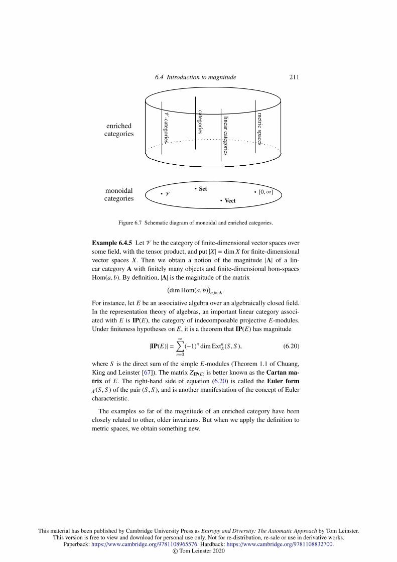
This material has been published by Cambridge University Press as Entropy and Diversity: The Axiomatic Approach by Tom Leinster.This version is free to view and download for personal use only. Not for re-distribution, re-sale or use in derivative works.
Paperback: https://www.cambridge.org/9781108965576. Hardback: https://www.cambridge.org/9781108832700.© Tom Leinster 2020
6.4 Introduction to magnitude 211
monoidalcategories
• V• Set
• Vect• [0,∞]
enrichedcategories
V-categories
categories
linearcategories
metric
spaces
Figure 6.7 Schematic diagram of monoidal and enriched categories.
Example 6.4.5 Let V be the category of finite-dimensional vector spaces oversome field, with the tensor product, and put |X| = dim X for finite-dimensionalvector spaces X. Then we obtain a notion of the magnitude |A| of a lin-ear category A with finitely many objects and finite-dimensional hom-spacesHom(a, b). By definition, |A| is the magnitude of the matrix(
dim Hom(a, b))a,b∈A.
For instance, let E be an associative algebra over an algebraically closed field.In the representation theory of algebras, an important linear category associ-ated with E is IP(E), the category of indecomposable projective E-modules.Under finiteness hypotheses on E, it is a theorem that IP(E) has magnitude
|IP(E)| =∞∑
n=0
(−1)n dim ExtnE(S , S ), (6.20)
where S is the direct sum of the simple E-modules (Theorem 1.1 of Chuang,King and Leinster [67]). The matrix ZIP(E) is better known as the Cartan ma-trix of E. The right-hand side of equation (6.20) is called the Euler formχ(S , S ) of the pair (S , S ), and is another manifestation of the concept of Eulercharacteristic.
The examples so far of the magnitude of an enriched category have beenclosely related to other, older invariants. But when we apply the definition tometric spaces, we obtain something new.

This material has been published by Cambridge University Press as Entropy and Diversity: The Axiomatic Approach by Tom Leinster.This version is free to view and download for personal use only. Not for re-distribution, re-sale or use in derivative works.
Paperback: https://www.cambridge.org/9781108965576. Hardback: https://www.cambridge.org/9781108832700.© Tom Leinster 2020
212 Species similarity and magnitude
Let V be the monoidal category [0,∞], with product +. For x ∈ [0,∞],define
|x| = e−x ∈ R.
(Recall that | · | is required to be ‘multiplicative’, that is, must convert the tensorproduct on V into multiplication. In this case, this means |x+y| = |x| · |y|, whichby Corollary 1.1.11(i) essentially forces |x| = cx for some constant c.) Then weobtain a notion of the magnitude of a finite V -category, and in particular, of afinite metric space.
In explicit terms, the definition is as follows. Let A = a1, . . . , an be a finitemetric space. Form the n × n matrix
ZA =(e−d(ai,a j)).
Invert ZA (if possible); then the magnitude |A| of A is the sum of all n2 entriesof Z−1
A .Here we have used Remark 6.3.11(ii) on the magnitude of a matrix in terms
of its inverse. Since ZA is a square matrix of real numbers, it is usually invert-ible, and in fact it is always invertible when A is a subspace of Euclidean space(Theorem 2.5.3 of Leinster [214] or Section 4 of Meckes [248]).
Examples 6.4.6 i. The magnitude of the zero-point space is 0, and the mag-nitude of the one-point space is 1.
ii. Consider the metric space A consisting of two points distance ` apart:
• oo` // •
Then
|A| = sum of entries of(e−0 e−`
e−` e−0
)−1
=2
1 + e−`,
as illustrated in Figure 6.8.This example can be understood as follows. When ` is small, the two
points are barely distinguishable, and may appear to be only one point (atpoor resolution, for instance). As ` increases, the two points acquire in-creasingly separate identities, and correspondingly, the magnitude increasestowards 2. In the extreme, when ` = ∞, the two points are entirely sepa-rated and the magnitude is exactly 2. This example and others suggest thatwe can usefully think of the magnitude of a finite metric space as the ‘effec-tive number of points’, or, more fully, the effective number of completelyseparate points.

This material has been published by Cambridge University Press as Entropy and Diversity: The Axiomatic Approach by Tom Leinster.This version is free to view and download for personal use only. Not for re-distribution, re-sale or use in derivative works.
Paperback: https://www.cambridge.org/9781108965576. Hardback: https://www.cambridge.org/9781108832700.© Tom Leinster 2020
6.4 Introduction to magnitude 213
0
1
2
0 1 2 3 4 5
`
|A|
Figure 6.8 The magnitude of a two-point space A, with points distance ` apart(Example 6.4.6(ii)).
`
1000`
1000`
A
0
1
2
3
0.0001 0.01 1 100
|A|
`
Figure 6.9 The magnitude of a certain three-point metric space A (Exam-ple 6.4.6(iv)). Note the logarithmic scale.
iii. Let A be a finite metric space in which all nonzero distances are ∞. ThenZA = I and |A| is just the cardinality of A. This also fits with the interpreta-tion of magnitude as the effective number of points.
iv. This example is adapted from Willerton ([354], Figure 1). Let A be a three-point space with the points arranged in a long thin triangle, as in Figure 6.9.When ` is small, the space appears to be just a single point, and the magni-tude is close to 1. When ` is moderate, the space appears to have two points,and the magnitude is about 2. When ` is large, the distinction between allthree points is clearly visible, and the magnitude is close to 3.
Empirical data such as this suggests a connection between magnitude andpersistent homology. Indeed, results of Otter [266] have begun to establishsuch a connection. We return to this topic at the end of the section.
Every metric space A belongs to a one-parameter family (tA)t>0 of spaces,where tA denotes A scaled up by a factor of t. So, magnitude assigns to eachfinite metric space A not just a number |A|, but a (partially-defined) function:
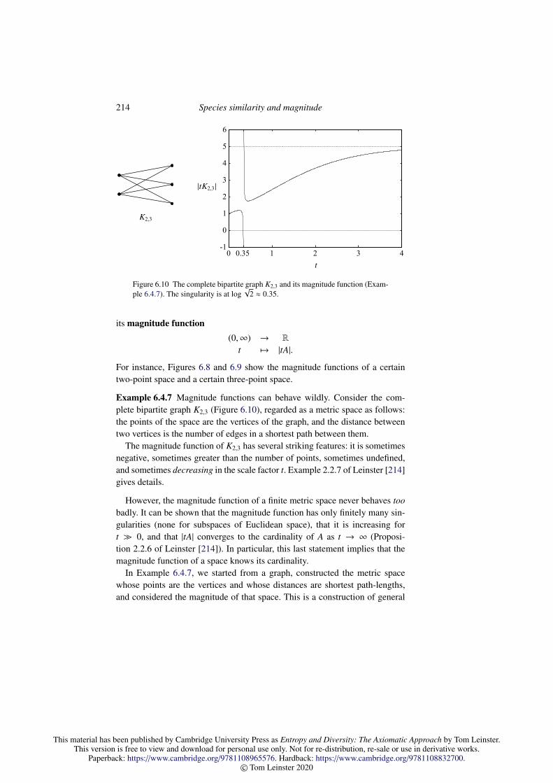
This material has been published by Cambridge University Press as Entropy and Diversity: The Axiomatic Approach by Tom Leinster.This version is free to view and download for personal use only. Not for re-distribution, re-sale or use in derivative works.
Paperback: https://www.cambridge.org/9781108965576. Hardback: https://www.cambridge.org/9781108832700.© Tom Leinster 2020
214 Species similarity and magnitude
K2,3
-1
0
1
2
3
4
5
6
0 0.35 1 2 3 4
t
|tK2,3|
Figure 6.10 The complete bipartite graph K2,3 and its magnitude function (Exam-ple 6.4.7). The singularity is at log
√2 ≈ 0.35.
its magnitude function(0,∞) → R
t 7→ |tA|.
For instance, Figures 6.8 and 6.9 show the magnitude functions of a certaintwo-point space and a certain three-point space.
Example 6.4.7 Magnitude functions can behave wildly. Consider the com-plete bipartite graph K2,3 (Figure 6.10), regarded as a metric space as follows:the points of the space are the vertices of the graph, and the distance betweentwo vertices is the number of edges in a shortest path between them.
The magnitude function of K2,3 has several striking features: it is sometimesnegative, sometimes greater than the number of points, sometimes undefined,and sometimes decreasing in the scale factor t. Example 2.2.7 of Leinster [214]gives details.
However, the magnitude function of a finite metric space never behaves toobadly. It can be shown that the magnitude function has only finitely many sin-gularities (none for subspaces of Euclidean space), that it is increasing fort 0, and that |tA| converges to the cardinality of A as t → ∞ (Proposi-tion 2.2.6 of Leinster [214]). In particular, this last statement implies that themagnitude function of a space knows its cardinality.
In Example 6.4.7, we started from a graph, constructed the metric spacewhose points are the vertices and whose distances are shortest path-lengths,and considered the magnitude of that space. This is a construction of general

This material has been published by Cambridge University Press as Entropy and Diversity: The Axiomatic Approach by Tom Leinster.This version is free to view and download for personal use only. Not for re-distribution, re-sale or use in derivative works.
Paperback: https://www.cambridge.org/9781108965576. Hardback: https://www.cambridge.org/9781108832700.© Tom Leinster 2020
6.4 Introduction to magnitude 215
interest, investigated in Leinster [215]. In this context, we replace the real num-ber e−1 in the definition of magnitude by a formal variable x. The magnitudeof a graph can then be expressed as either a rational function or a power seriesin x with integer coefficients (Section 2 of [215]). For example, the graphs
all have magnitude
5 + 5x − 4x2
(1 + x)(1 + 2x)= 5 − 10x + 16x2 − 28x3 + 52x4 − 100x5 + · · ·
(Example 4.11 of [215]). The magnitude of a graph shares some invarianceproperties with one of the most important graph invariants of all, the Tuttepolynomial. For instance, it is invariant under Whitney twists when the pointsof identification are adjacent. But it is not a specialization of the Tutte polyno-mial: it carries information that the Tutte polynomial does not.
Graph magnitude satisfies multiplicativity and inclusion-exclusion princi-ples:
|G × H| = |G| · |H|,
|G ∪ H| = |G| + |H| − |G ∩ H|
(where the latter is under quite strict hypotheses), shown as Lemma 3.6 andTheorem 4.9 of Leinster [215]. As such, it has a reasonable claim to being thegraph-theoretic analogue of cardinality.
As additional evidence for this claim, Hepworth and Willerton [142] con-structed a graded homology theory of graphs whose Euler characteristic ismagnitude. In more detail: since their homology theory is graded, the Eulercharacteristic of a graph is not a single number but a sequence of numbers,which when construed as a power series is exactly the graph’s magnitude.Thus, their homology theory is a categorification of magnitude in the samesense that the Khovanov homology of knots and links [187] is a categorifica-tion of the Jones polynomial. It is a finer invariant than magnitude, in that thereare graphs with the same magnitude but different homology groups (Gu [131],Appendix A; see also Summers [318]).
Not only the definition of magnitude for graphs, but also some theoremsabout it, can be categorified. For instance, Hepworth and Willerton provedthat the multiplicativity and inclusion-exclusion theorems for magnitude liftto Kunneth and Mayer–Vietoris theorems in homology. In this sense, knownproperties of the magnitude of graphs are shadows of functorial results in ho-mology.

This material has been published by Cambridge University Press as Entropy and Diversity: The Axiomatic Approach by Tom Leinster.This version is free to view and download for personal use only. Not for re-distribution, re-sale or use in derivative works.
Paperback: https://www.cambridge.org/9781108965576. Hardback: https://www.cambridge.org/9781108832700.© Tom Leinster 2020
216 Species similarity and magnitude
Hepworth and Willerton’s idea even works in the full generality of enrichedcategories. That is, the magnitude of an enriched category (a numerical invari-ant) can be categorified to a graded homology theory for enriched categories(an algebraic invariant). As in the case of graphs, ‘categorified’ means that theEuler characteristic of the homology theory is exactly magnitude. This mag-nitude homology for enriched categories was defined and developed in workled by Shulman [222]. It is a kind of Hochschild homology.
Since metric spaces are a special kind of enriched category, this constructionprovides a new homology theory for metric spaces. It is genuinely metric ratherthan topological. For example, the first magnitude homology of a closed subsetX of Rn is trivial if and only if X is convex ([222], Section 4). Indeed, all ofthe magnitude homology groups of a convex subset of Rn are trivial, a metricanalogue of the topological fact that the homology of a contractible space istrivial. This was proved independently by Kaneta and Yoshinaga (Corollary 5.3of [174]) and by Jubin (Theorem 7.2 of [172]). Gomi [117] states a slogan:
The more geodesics are unique, the more magnitude homology is trivial.
Methods for computing the magnitude homology of metric spaces haverecently been developed and applied to calculate specific homology groups.Gomi developed spectral sequence techniques and used them to prove resultson the magnitude homology groups of circles ([118], Section 4). Kaneta andYoshinaga [174] showed that while ordinary topological homology detects theexistence of holes, magnitude homology detects the diameter of holes, in asense made precise in their Theorem 5.7. Asao proved that if a space contains aclosed geodesic then its second magnitude homology group is nontrivial (The-orem 5.3 of [19]), while Gomi [117] proved general results on the second andthird magnitude homology groups of metric spaces.
Magnitude homology is not the first homology theory of metric spaces: thereis also persistent homology, fundamental in the field of topological data analy-sis. (For expository accounts of persistent homology, see Ghrist [113] or Carls-son [59].) Otter [266] has proved results relating the two homology theories,introducing for this purpose a notion of ‘blurred magnitude homology’; seealso Govc and Hepworth [123] and Cho [66].
Finally, Hepworth [141] has introduced a theory of magnitude cohomologyfor enriched categories. It carries a product that formally resembles the ordi-nary cup product, but is noncommutative. For finite metric spaces, magnitudecohomology is a complete invariant: the cohomology ring of such a space de-termines it uniquely up to isometry.

This material has been published by Cambridge University Press as Entropy and Diversity: The Axiomatic Approach by Tom Leinster.This version is free to view and download for personal use only. Not for re-distribution, re-sale or use in derivative works.
Paperback: https://www.cambridge.org/9781108965576. Hardback: https://www.cambridge.org/9781108832700.© Tom Leinster 2020
6.5 Magnitude in geometry and analysis 217
6.5 Magnitude in geometry and analysis
Most metric spaces of geometric interest are not finite. The general enriched-categorical concept of magnitude provides no definition of the magnitude of aninfinite metric space. On the other hand, there are several plausible strategiesfor extending the definition of magnitude from finite to compact metric spaces.Meckes [248, 249] showed that as long as the space satisfies a certain classicalcondition, they all give the same outcome.
The condition is that the space must be of negative type. We do not need theoriginal definition here, but Meckes refined old results of Schoenberg [304] toshow that A is of negative type if and only if the matrix ZtB is positive definitefor every finite B ⊆ A and real t > 0 (Theorem 3.3 of [248]). A great manyspaces are of negative type, including all subspaces of Rn with the Euclidean or`1 (taxicab) metric, all ultrametric spaces, real and complex hyperbolic space,and spheres with the geodesic metric. A list can be found in Theorem 3.6of [248].
The most direct way to state the extended definition of magnitude is as fol-lows.
Definition 6.5.1 Let A be a compact metric space of negative type. The mag-nitude of A is
|A| = sup|B| : finite subsets B ⊆ A ∈ [0,∞].
Equivalently, one can choose a sequence B1 ⊆ B2 ⊆ · · · ⊆ A of finite sub-spaces Bn of A such that
⋃Bn is dense in A, then put |A| = limn→∞|Bn|. Equiv-
alently again, one can define the magnitude of A by the variational formula
|A| = supµ
µ(A)2∫A
∫A e−d(a,b) dµ(a) dµ(b)
, (6.21)
where the supremum is over the finite signed Borel measures µ on A for whichthe denominator is nonzero.
This last characterization is related to yet another formulation. A weightmeasure on A is a finite signed Borel measure µ such that∫
Ae−d(a,b) dµ(b) = 1
for all a ∈ A. This definition was introduced by Willerton ([352], Section 1.1),and is the continuous analogue of the notion of weighting (Definition 6.3.8). Ifµ is a weight measure on A then |A| = µ(A), by Theorem 2.3 of Meckes [248] orProposition 5.3.6 of Leinster and Meckes [220]. However, not every compact

This material has been published by Cambridge University Press as Entropy and Diversity: The Axiomatic Approach by Tom Leinster.This version is free to view and download for personal use only. Not for re-distribution, re-sale or use in derivative works.
Paperback: https://www.cambridge.org/9781108965576. Hardback: https://www.cambridge.org/9781108832700.© Tom Leinster 2020
218 Species similarity and magnitude
metric space of negative type admits a weight measure. Most weightings aredistributions of a more general kind, defined in Meckes [249].
The equivalence of these and other definitions of magnitude was establishedby Meckes [248, 249], using techniques of harmonic and functional analysis.
We now give some examples of compact spaces A and their magnitude func-tions t 7→ |tA|.
Example 6.5.2 The magnitude function of a straight line [0, `] of length ` isgiven by
|t · [0, `]| = 1 + 12` · t.
Several proofs are known, as in Theorem 7 of Leinster and Willerton [223],Theorem 2 of Willerton [352], and Proposition 3.2.1 of Leinster [214]. Theeasiest proof uses weight measures. Let δ0 and δ` denote the point measures at0 and `, let λ[0,`] denote Lebesgue measure on [0, `], and put
µ = 12 (δ0 + λ[0,`] + δ`).
It is easily verified that µ is a weight measure on [0, `]. Hence
|[0, `]| = 1 + 12`,
and so the magnitude function of [0, `] is given by
|t · [0, `]| = 1 + 12` · t.
Example 6.5.3 Magnitude is multiplicative with respect to the `1 product ofmetric spaces, that is, the product space with the metric given by adding thedistances in the two factors (Proposition 3.1.4 of Leinster [214]). This has thefollowing consequence. Equip Rn with the `1 metric:
d(x, y) =
n∑i=1
|xi − yi|
(x, y ∈ Rn). Then by the previous example, the magnitude function of a rectan-gle
A = [0, `] × [0,m] ⊆ R2
is given by
|tA| =(1 + 1
2` · t)(
1 + 12 m · t
)= 1 + 1
2 (` + m) · t + 14`m · t
2.
Up to a constant factor, the coefficient of t2 is the area of A, the coefficientof t is the perimeter of A, and the constant term is the Euler characteristic of
This material has been published by Cambridge University Press as Entropy and Diversity: The Axiomatic Approach by Tom Leinster.This version is free to view and download for personal use only. Not for re-distribution, re-sale or use in derivative works.
Paperback: https://www.cambridge.org/9781108965576. Hardback: https://www.cambridge.org/9781108832700.© Tom Leinster 2020
6.5 Magnitude in geometry and analysis 219
A. Similar statements apply to higher-dimensional boxes (Corollary 3.4.3 ofLeinster [214]).
For rectangles, and for nonempty convex sets in general, the Euler charac-teristic is always 1. As such, it may seem pretentious to call the constant termthe ‘Euler characteristic’. This usage will be justified shortly.
To begin to explain the geometric content of magnitude, we need to recall theconcept of intrinsic volumes (Klain and Rota [188] or Section 4.1 of Schnei-der [303]), which with different normalizations are also known as quermassin-tegrals or Minkowski functionals.
Consider all reasonable ways of measuring the size of compact convex sub-sets of Rn (which in the present discussion will just be called convex sets). Inthe plane R2, there are at least three ways to measure a set: take its area, itsperimeter, or its Euler characteristic. These are 2-, 1-, and 0-dimensional mea-sures, respectively. The general fact is that there are n + 1 canonical ways ofmeasuring convex subsets of Rn, which define functions
V0, . . . ,Vn : convex subsets of Rn → R.
Here Vi is i-dimensional, in the sense that Vi(tA) = tiVi(A), and Vi(A) is calledthe ith intrinsic volume of A.
The ith intrinsic volume of a convex set A ⊆ Rn can be defined as fol-lows. Choose at random an i-dimensional linear subspace L of Rn, take theorthogonal projection πL(A) of A onto L, then take its i-dimensional volumeVol(πL(A)). Up to a constant factor, Vi(A) is the expected value of Vol(πL(A)).
Example 6.5.4 Let A be a convex subset of R3. Then V0(A) is 0 if A is empty,and 1 otherwise. (In both cases, V0(A) is the Euler characteristic of A.) The firstintrinsic volume V1(A) is proportional to the expected length of the projectionof A onto a random line, and is called the mean width of A. The second in-trinsic volume V2(A) is proportional to the expected area of the projection of Aonto a random plane, and it is a theorem of Cauchy that this is proportional tothe surface area of A (Klain and Rota [188], Theorem 5.5.2). Finally, V3(A) isjust the volume of A.
Each of the intrinsic volumes Vi on convex sets is isometry-invariant, con-tinuous with respect to the Hausdorff metric, and a valuation: Vi(∅) = 0 and
Vi(A ∪ B) = Vi(A) + Vi(B) − Vi(A ∩ B)
whenever A, B and A∪ B are convex. The same is, therefore, true of any linearcombination of the intrinsic volumes. A celebrated theorem of Hadwiger [132]
This material has been published by Cambridge University Press as Entropy and Diversity: The Axiomatic Approach by Tom Leinster.This version is free to view and download for personal use only. Not for re-distribution, re-sale or use in derivative works.
Paperback: https://www.cambridge.org/9781108965576. Hardback: https://www.cambridge.org/9781108832700.© Tom Leinster 2020
220 Species similarity and magnitude
states that such linear combinations are the only isometry-invariant continuousvaluations on convex sets.
The intrinsic volumes can be adapted to more general classes of space and todifferent geometries. For instance, we can speak of the volume or surface areaof a sufficiently smooth subset of Rn, and in that context, the intrinsic volumesare closely related to curvature measures. (See Section 2.1.1 of Alesker andFu [8] for a concise review of the relationship, Morvan [253] or Gray [125]for full accounts of curvature measures, and Alesker [6] for a survey of somemore recent developments.) The intrinsic volumes can also be defined on anyfinite union of convex sets (as in Klain and Rota [188]). At these levels ofgenerality, V0 is no longer trivial; it is the Euler characteristic. This justifies‘Euler characteristic’ as the right name for V0 even in the case of convex sets.
The next example uses a notion of intrinsic volume adapted to Rn with the`1 metric.
Example 6.5.5 Generalizing Example 6.5.3, let A ⊆ Rn be a convex body,that is, a convex set with nonempty interior. Give A the `1 metric. Then themagnitude function of A is the polynomial
|tA| =n∑
i=0
12i V ′i (A) · ti
(Theorem 5.4.6(2) of Leinster and Meckes [220]). Here V ′i (A) is the `1 ana-logue of the ith intrinsic volume of A, discussed in [220] and in Section 5 ofLeinster [211]. Explicitly, it is the sum of the i-dimensional volumes of theprojections of A onto the i-dimensional coordinate subspaces of Rn. The sig-nificance of 2i is that the volume of the unit ball in the 1-norm on Rn is 2i/i!.
So, for convex bodies inRn equipped with the `1 metric, the magnitude func-tion is a polynomial whose degree is the dimension and whose ith coefficientis an i-dimensional geometric measure.
For the Euclidean rather than `1 metric on Rn, results on magnitude areharder. Until 2015, the only convex subset of Rn whose magnitude was knownwas the line segment. But a significant advance was made by Barcelo andCarbery [28], who used PDE methods to prove:
Theorem 6.5.6 (Barcelo and Carbery) Let n ≥ 1 be odd. Then:
i. the magnitude function t 7→ |tBn| of the n-dimensional unit Euclidean ballBn is a rational function over Z of the radius t;
This material has been published by Cambridge University Press as Entropy and Diversity: The Axiomatic Approach by Tom Leinster.This version is free to view and download for personal use only. Not for re-distribution, re-sale or use in derivative works.
Paperback: https://www.cambridge.org/9781108965576. Hardback: https://www.cambridge.org/9781108832700.© Tom Leinster 2020
6.5 Magnitude in geometry and analysis 221
ii. the magnitude functions of B1, B3 and B5 are given by
|tB1| = 1 + t,
|tB3| =13!
(6 + 12t + 6t2 + t3),
|tB5| =15!
360 + 1080t + 525t2 + 135t4 + 18t5 + t6
3 + t.
Proof Part (i) is Theorem 4 of [28]. For part (ii), the formulas for |tB3| and |tB5|
are Theorems 2 and 3 of [28], and the formula for |tB1| is Example 6.5.2 (notdue to Barcelo and Carbery, but included in the statement for completeness).
In the `1 metric on Rn, the magnitude of a ball is a polynomial in its ra-dius, by Example 6.5.5. In the Euclidean metric, it is no longer a polynomial,but it is the next best thing: a rational function. Subsequent work of Willer-ton [356, 355] identified exactly which rational function |tBn| is, in terms ofBessel polynomials and Hankel determinants.
Theorem 6.5.6 is stated under the hypothesis that n is odd, a condition im-posed in order to put the proof into the realm of differential rather than pseu-dodifferential equations. The magnitude of even-dimensional balls remains un-known. Even the 2-dimensional disc B2 has unknown magnitude, although nu-merical experiments suggest that it is a certain quadratic polynomial in theradius (Willerton [350], Section 3.2).
Barcelo and Carbery also proved a result on general compact sets (Theo-rem 1 of [28]):
Theorem 6.5.7 (Barcelo and Carbery) For all n ≥ 1 and compact A ⊆ Rn,
Vol(A) = cn limt→∞
|tA|tn ,
where the constant cn is n! Vol(Bn).
The volume of the Euclidean unit ball Bn is given by a standard classical for-mula, as in Propositions 6.2.1 and 6.2.2 of Klain and Rota [188], for instance.
By Theorem 6.5.7, we can extract the volume of a set from its magnitudefunction. This substantiates the earlier claim that the general notion of the mag-nitude of an enriched category encompasses the notion of volume.
Better still, using methods of global analysis, Gimperlein and Goffengproved (Theorem 2(d) of [115]):
Theorem 6.5.8 (Gimperlein and Goffeng) Let n ≥ 1 be odd, and let A ⊆ Rn
be a bounded set with smooth boundary such that A is the closure of its interior.

This material has been published by Cambridge University Press as Entropy and Diversity: The Axiomatic Approach by Tom Leinster.This version is free to view and download for personal use only. Not for re-distribution, re-sale or use in derivative works.
Paperback: https://www.cambridge.org/9781108965576. Hardback: https://www.cambridge.org/9781108832700.© Tom Leinster 2020
222 Species similarity and magnitude
Then the magnitude function of A has an asymptotic expansion
|tA| ∼∞∑
i=0
mi(A)tn−i as t → ∞,
and up to a known constant factor (depending on n and i but not A), the coef-ficient mi(A) is equal to the intrinsic volume Vn−i(A) for i = 0, 1, 2.
Recent work of Gimperlein, Goffeng and Louca, so far unpublished, re-moves the restriction that n is odd.
For instance, m0(A) = Vol(A)/n! Vol(Bn) (as in Theorem 6.5.7) and m1(A) isproportional to the (n − 1)-dimensional surface area of A. In the statement ofTheorem 6.5.8, the term ‘intrinsic volume’ has been extended beyond its usualcontext of convex sets. A more precise statement for i = 2 is that m2(A) isproportional to the integral over ∂A of the mean curvature of ∂A (which whenA is convex is itself proportional to Vn−2(A)).
The magnitude of a metric space does not satisfy the inclusion-exclusionprinciple in the strongest conceivable sense, since otherwise, every n-pointspace would have magnitude n. But Gimperlein and Goffeng showed thatmagnitude does satisfy inclusion-exclusion in an asymptotic sense, using tech-niques related to the heat equation proof of the Atiyah–Singer index theoremand making essential use of complex scale factors t. Indeed, for subsets A, Band A ∩ B of Rn satisfying the regularity conditions of Theorem 6.5.8,
|t(A ∪ B)| + |t(A ∩ B)| − |tA| − |tB| → 0 as t → ∞
(Remark 3 of [115]). This is further evidence for the claim that magnitudeshould be regarded as a measure of size.
Finally, we return to diversity. Meckes defined the maximum diversity of acompact space A of negative type as
Dmax(A) = supµ
1∫A
∫A e−d(a,b) dµ(a) dµ(b)
,
which is similar to the formula (6.21) for magnitude, except that now the supre-mum runs over only the Borel probability measures µ, as opposed to all signedmeasures. (In principle, the formula is for the maximum diversity of order 2,but Theorem 7.1 of Leinster and Roff [221] implies that the maximum diversityof every order is the same.) Evidently Dmax(A) ≤ |A|.
When A is a subset of Euclidean space, Dmax(A) is equal to a classical quan-tity, the Bessel capacity C(n+1)/2(A). As Meckes showed, a deep result fromthe theory of capacities provides an upper bound on |A|/Dmax(A) in terms ofn alone (Corollary 6.2 of [249]). Thus, magnitude is never very different fromthis Bessel capacity.
This material has been published by Cambridge University Press as Entropy and Diversity: The Axiomatic Approach by Tom Leinster.This version is free to view and download for personal use only. Not for re-distribution, re-sale or use in derivative works.
Paperback: https://www.cambridge.org/9781108965576. Hardback: https://www.cambridge.org/9781108832700.© Tom Leinster 2020
6.5 Magnitude in geometry and analysis 223
Meckes [249] exploited the connection between magnitude and maximumdiversity to extract information about the dimension of a compact set A ⊆ Rn
from its magnitude function. We have already met some families of spaceswhere the magnitude function is a polynomial whose degree is the dimension(Example 6.5.5). But here we allow non-integer dimensions too.
One of the most important notions of fractional dimension is the Minkowskior box-counting dimension (Section 3.1 of Falconer [96]). The Minkowskidimension of a subset of Rn is always greater than or equal to the Hausdorffdimension, and equality often holds. (See p. 43 of [96] for a summary of howthe two dimensions are related.) For instance, both the Minkowski and theHausdorff dimensions of the middle-thirds Cantor set are log 2/ log 3. WritedimM A for the Minkowski dimension of a compact set A ⊆ Rn, if defined.
Roughly speaking, the following result states that |tA| grows like tdimM A
when t is large. Thus, we can can recover the Minkowski dimension of a spacefrom its magnitude function. It is due to Meckes (Corollary 7.4 of [249]).
Theorem 6.5.9 (Meckes) Let A be a compact subset of Rn. Then
dimM A = limt→∞
log|tA|log t
,
with one side of the equation defined if and only if the other is.
For instance, if A is a subset of Rn with nonzero volume, then |tA| growslike tn when t is large, and by the volume theorem of Barcelo and Carbery, theratio |tA|/tn converges to a known constant times the volume of A. When A isthe middle-thirds Cantor set, |tA| grows like tlog 2/ log 3. (In fact, the magnitudefunction of the Cantor set also has a kind of hidden periodicity, as shown inSection 3 of Leinster and Willerton [223].) For convex subsets of Rn, moreprecise statements can be made; Meckes bounds the magnitude function of aconvex set by a polynomial whose coefficients are proportional to its intrinsicvolumes ([250], Theorem 1).
Theorem 6.5.9 demonstrates the usefulness of the concept of maximum di-versity for pure-mathematical purposes in geometry and analysis, indepen-dently of any biological application.

This material has been published by Cambridge University Press as Entropy and Diversity: The Axiomatic Approach by Tom Leinster.This version is free to view and download for personal use only. Not for re-distribution, re-sale or use in derivative works.
Paperback: https://www.cambridge.org/9781108965576. Hardback: https://www.cambridge.org/9781108832700.© Tom Leinster 2020
7
Value
Quite apart from many theoretical and practical problems that continueto affect the species concept and its application, is it appropriate for con-servation purposes to regard all species as equal in this manner? To aconservationist, regardless of relative abundance, is Welwitschia equal toa species of Taraxacum? Is the panda equivalent to one species of rat?
– Vane-Wright et al. ([339], p. 237)
Putting aside entropy and diversity, let us consider a very general question:
What is the value of the whole in terms of its parts?
Although the question in this form is far too vague to admit a mathematicaltreatment, we will see that once posed precisely, it has a complete answer.From that answer, the concept of diversity arises automatically. The answeralso leads to a unique characterization of the Hill numbers (or equivalently,the Renyi entropies), more powerful than the characterization theorem in Sec-tion 4.5.
We will consider a ‘whole’ divided into n ‘parts’ of relative sizes p1, . . . , pn,which are assigned values v1, . . . , vn respectively (Figure 7.1). The question ishow to aggregate those values into a single value σ(p, v) for the whole, mea-
p1
v1np2
v2np3
v3n p4v4np5
v5n
Figure 7.1 A whole divided into 5 parts, with relative sizes (p1, . . . , p5) ∈ ∆5 andvalues (v1, . . . , v5).
224
This material has been published by Cambridge University Press as Entropy and Diversity: The Axiomatic Approach by Tom Leinster.This version is free to view and download for personal use only. Not for re-distribution, re-sale or use in derivative works.
Paperback: https://www.cambridge.org/9781108965576. Hardback: https://www.cambridge.org/9781108832700.© Tom Leinster 2020
Value 225
sured in the same units as the values vi of the parts. This aggregation methodshould have sensible properties. For instance, if we put together two parts ofequal size and equal value, v, the result should have value 2v.
One simple method is to ignore the sizes of the parts and just sum theirvalues, so that
σ(p, v) = v1 + · · · + vn
(or better,σ(p, v) =∑
i∈supp(p) vi). But there are many other possibilities. In fact,we will define a one-parameter family (σq) of value measures. They include asspecial cases the Hill numbers Dq, the more general similarity-sensitive diver-sity measures DZ
q of Chapter 6, certain phylogenetic diversity measures (due toChao, Chiu and Jost [65]), and, essentially, the `p norms. For example, when acommunity is divided into n species in proportions p1, . . . , pn, and each speciesis assigned the same value, 1, the value of the whole according to σq is the Hillnumber of order q:
σq(p, (1, . . . , 1)
)= Dq(p).
In most of the cases just listed, the whole is taken to be an ecological com-munity and the parts are its species. But there is an important complementarysituation, in which the whole is still a community but the parts are taken tobe subcommunities. For instance, the community might be divided geographi-cally into regions, and we might attempt to evaluate the community as a wholebased on the sizes and values of those regions. In the case where value is inter-preted as diversity, that is exactly what we did when we derived the chain rulefor diversity (Propositions 4.4.10 and 6.2.11). Indeed, the function σq can beseen as an embodiment of the chain rules for Dq and DZ
q , in a sense explainedin Example 7.1.8.
We begin by defining the value measures σq and analysing some specialcases (Section 7.1), with important examples from both ecology and the analy-sis of social welfare. We then introduce the Renyi relative entropies, which arevery closely related to the value measures σq. (The q-logarithmic relative en-tropies were already covered in Section 4.1.) As a bonus, we use the Renyi andq-logarithmic relative entropies to provide further evidence for the canonicalnature of the Fisher metric on probability distributions (Remark 7.2.3(i)).
Using our earlier results on means, we then prove that the only value mea-sures with reasonable properties are those belonging to the family (σq) (Sec-tion 7.3). From this we deduce that for communities modelled as their relativeabundance distributions, the only reasonable measures of diversity are the Hillnumbers (Section 7.4).
We have already proved a characterization theorem for the Hill numbers Dq

This material has been published by Cambridge University Press as Entropy and Diversity: The Axiomatic Approach by Tom Leinster.This version is free to view and download for personal use only. Not for re-distribution, re-sale or use in derivative works.
Paperback: https://www.cambridge.org/9781108965576. Hardback: https://www.cambridge.org/9781108832700.© Tom Leinster 2020
226 Value
in Section 4.5, showing that for a fixed q, if a diversity measure D has certainproperties depending on q, then it must be equal to Dq. But in the theoremproved in this chapter, there is no ‘q’ mentioned in the hypotheses, and theconclusion is that D must be equal to Dq for some q. In short, the earlier theo-rem characterized the Hill numbers individually, but this theorem characterizesthem as a family.
7.1 Introduction to value
Here we consider sequences of functions(σ : ∆n × [0,∞)n → [0,∞)
)n≥1,
which will be referred to as value measures. We regard a pair (p, v) ∈∆n × [0,∞)n as representing a whole made up of n disjoint parts with rela-tive sizes p1, . . . , pn and values v1, . . . , vn, and we regard σ(p, v) as the valuethat σ assigns to the whole.
A special role is played by the family(σq
)q∈[−∞,∞]
of value measures, defined by
σq(p, v) = M1−q(p, v/p)
(n ≥ 1, p ∈ ∆n, v ∈ [0,∞)n). The convention adopted in Remark 4.2.15 ensuresthat σq(p, v) is always well-defined. We call σq the value measure of orderq. Explicitly, when q , 1,±∞,
σq(p, v) =
( ∑i∈supp(p)
pqi v1−q
i
)1/(1−q)
,
unless q > 1 and vi = 0 for some i ∈ supp(p), in which case σq(p, v) = 0. Forq ∈ 1,±∞,
σ−∞(p, v) = maxi∈supp(p)
vi
pi,
σ1(p, v) =∏
i∈supp(p)
( vi
pi
)pi
,
σ∞(p, v) = mini∈supp(p)
vi
pi.
Examples 7.1.1 i. Consider a set of k individuals, divided into n equivalenceclasses (‘parts’), with the ith part consisting of ki individuals. Let pi = ki/k

This material has been published by Cambridge University Press as Entropy and Diversity: The Axiomatic Approach by Tom Leinster.This version is free to view and download for personal use only. Not for re-distribution, re-sale or use in derivative works.
Paperback: https://www.cambridge.org/9781108965576. Hardback: https://www.cambridge.org/9781108832700.© Tom Leinster 2020
7.1 Introduction to value 227
be the proportion of individuals in the ith part. Let v1, . . . , vn ∈ [0,∞) beany values assigned to the parts. Then
σq(p, v) = M1−q
(p,
(kv1
k1, . . . ,
kvn
kn
)),
or equivalently,
σq(p, v) = k · M1−q
(p,
(v1
k1, . . . ,
vn
kn
)). (7.1)
This can be understood as follows. If the value vi of the ith part is sharedout evenly among its ki members, then the value per individual in the ithpart is vi/ki. Hence the mean value per individual in the whole is
M1−q
(p,
(v1
k1, . . . ,
vn
kn
)).
So, equation (7.1) states that
value of whole = number of individuals ×mean value per individual.
This is the basic conceptual relationship between value measures andmeans.
ii. If in (i) we interpret ‘mean’ as arithmetic mean, then we are in the caseq = 0, and σ0 is simply given by
σ0(p, v) =∑
i∈supp(p)
vi
(as in the introduction to this chapter). But we have seen repeatedly in thisbook that the arithmetic mean is not the only useful kind. The other powermeans should always be considered alongside it, and in this case, they givethe whole family (σq).
Remark 7.1.2 The value measures σq and the power means Mt are sequencesof functions of the same type:(
σq,Mt : ∆n × [0,∞)n → [0,∞))n≥1.
However, Example 7.1.1(i) makes clear that there should be no overlap be-tween the classes of value measures and means. Indeed, a reasonable valuemeasure σ should satisfy
σ(un, (v, . . . , v)
)= nv,
whereas a minimal requirement of a mean M is the consistency condition
M(un, (x, . . . , x)
)= x.

This material has been published by Cambridge University Press as Entropy and Diversity: The Axiomatic Approach by Tom Leinster.This version is free to view and download for personal use only. Not for re-distribution, re-sale or use in derivative works.
Paperback: https://www.cambridge.org/9781108965576. Hardback: https://www.cambridge.org/9781108832700.© Tom Leinster 2020
228 Value
So, no reasonable mean is a reasonable value measure. We return to the rela-tionship between means and value measures in Section 7.3.
For positive parameters q, the value of the whole is never more than the sumof the values of its parts:
Lemma 7.1.3 For all q ≥ 0, p ∈ ∆n, and v ∈ [0,∞)n,
σq(p, v) ≤n∑
i=1
vi.
For q > 0, equality holds if and only if v is a scalar multiple of p.
So for fixed∑
vi, the value of the whole is maximized when value is spreadevenly across the constituent parts, in proportion to their sizes.
Proof For all q ≥ 0,
σq(p, v) = M1−q(p, v/p) ≤ M1(p, v/p) =∑
i∈supp(p)
vi ≤
n∑i=1
vi.
Assuming now that q > 0, equality holds in the first inequality if and only ifvi/pi is constant over i ∈ supp(p) (by Theorem 4.2.8), and in the second if andonly if vi = 0 for all i < supp(p). The result follows.
The next two examples illuminate the meaning of the parameter q. Theyconcern the case where the parts are of equal size (p = un), so that the valuemeasures σq are given by
σq(un, v) = n · M1−q(un, v)
(q ∈ [−∞,∞], v ∈ [0,∞)n).
Example 7.1.4 A classical question in welfare economics is how to take agroup of agents, each of which has an assigned utility, and aggregate theirindividual utilities into a measure of the utility of the group as a whole. For in-stance, the agents might be the citizens of a society, and the utility of a citizenmight be their individual level of welfare, wealth or well-being. The challenge,then, is to combine them into a single number representing the collective wel-fare of the society. (As a general reference for all of this example, we refer toSection 1.2 and Chapter 3 of Moulin [254].)
Specifically, fix n, and take a group of n individuals with respective utilitiesv1, . . . , vn ≥ 0. A collective utility function assigns a real number f (v) to eachsuch tuple v = (v1, . . . , vn). For example,
σq(un,−) : [0,∞)n → R
This material has been published by Cambridge University Press as Entropy and Diversity: The Axiomatic Approach by Tom Leinster.This version is free to view and download for personal use only. Not for re-distribution, re-sale or use in derivative works.
Paperback: https://www.cambridge.org/9781108965576. Hardback: https://www.cambridge.org/9781108832700.© Tom Leinster 2020
7.1 Introduction to value 229
is a collective utility function for each q ∈ [−∞,∞].More important than the collective utility function f itself is its associated
social welfare ordering, which is the relation on [0,∞)n defined by
v v′ ⇐⇒ f (v) ≤ f (v′).
In the case of the welfare of the citizens of a society, v v′ is interpreted as thejudgement that when the welfare levels of the citizens are v1, . . . , vn, society isin a poorer state than when they are v′1, . . . , v
′n.
Of course, such judgements depend on a choice of collective utility functionf . When f = σq(un,−), different values of q correspond to different view-points, some of which are associated with particular schools of political phi-losophy. The case q = 0 is
σ0(un,−) : v 7→∑
vi,
so that the collective welfare is simply the sum of the individual welfares. Thisfunction is associated with classical utilitarianism, with its roots in the philos-ophy of Jeremy Bentham and in John Stuart Mill’s ‘sum total of happiness’.When q = ∞, the collective utility function is
σ∞(un,−) : v 7→ n min vi,
so that
v v′ ⇐⇒ min vi ≤ min v′i .
This viewpoint on collective welfare is associated with the philosophy of JohnRawls: a society should be judged by the welfare of its most miserable citizen.An intermediate position is q = 1, where
σ1(un,−) : v 7→ n ·(∏
vi
)1/n
and so
v v′ ⇐⇒∏
vi ≤∏
v′i .
In this context, the product operation v 7→∏
vi is known as the Nash collectiveutility function, and has special properties not shared by any other collectiveutility function (unsurprisingly, given the special role played by the case q = 1in the context of entropy).
An important property of collective utility functions is the Pigou–Daltonprinciple. In the language of wealth, this states that transferring a small amountof wealth from a richer citizen to a poorer one is beneficial to the overall wel-fare of society. Formally, let v ∈ [0,∞)n and i, j ∈ 1, . . . , n with vi < v j, and
This material has been published by Cambridge University Press as Entropy and Diversity: The Axiomatic Approach by Tom Leinster.This version is free to view and download for personal use only. Not for re-distribution, re-sale or use in derivative works.
Paperback: https://www.cambridge.org/9781108965576. Hardback: https://www.cambridge.org/9781108832700.© Tom Leinster 2020
230 Value
let 0 ≤ δ ≤ (v j − vi)/2; define v′ ∈ [0,∞)n by
v′k =
vi + δ if k = i,
v j − δ if k = j,
vk otherwise.
The Pigou–Dalton principle is that v v′ for all such v, i, j, and δ.When q ∈ [0,∞], an elementary calculation shows that σq(un,−) satisfies
the Pigou–Dalton principle. Thus, redistribution is regarded positively. On theother hand, the Pigou–Dalton principle fails for all q ∈ [−∞, 0). In fact, for q ∈(−∞, 0), redistribution from richer to poorer always strictly decreases overallwelfare. In the extreme case q = −∞, the collective utility function is
σ−∞(un,−) : v 7→ n maxi
vi,
so that the welfare of a society is proportional to the welfare of its most priv-ileged citizen. (Recall that n is fixed.) Thus, from the viewpoint of q = −∞,collective welfare is optimized when all the wealth is transferred to a singleindividual. In the welfare economics literature, negative values of q are oftenexcluded.
(The family (σq(un,−)) of collective utility functions that we have used isdifferent from the family used in economics texts such as Moulin [254], butonly superficially. In the literature, it is conventional to use the functions
v 7→∑
vti (t ∈ (0,∞)),
v 7→∑
log vi,
v 7→ −∑
vti (t ∈ (−∞, 0)),
whereas we have been using
v 7→ σq(un, v) =
nq/(q−1)(∑
v1−qi
)1/(1−q)if 1 , q ∈ (−∞,∞),
n∏
v1/ni if q = 1.
(7.2)
But reparametrizing with q = 1 − t, the induced social welfare orderings areidentical.)
Example 7.1.5 In contexts such as collective welfare and diversity, it is naturalto restrict the parameter q to be positive. But for negative parameters q, thevalue measures σq also define something important, at least when the parts areof equal size: the `p norms. Indeed, for −∞ < q ≤ 0, equation (7.2) gives
σq(un, v) = nq/(q−1)‖v‖1−q,
where the norm ‖ · ‖1−q is as defined in Example 9.3.2.
This material has been published by Cambridge University Press as Entropy and Diversity: The Axiomatic Approach by Tom Leinster.This version is free to view and download for personal use only. Not for re-distribution, re-sale or use in derivative works.
Paperback: https://www.cambridge.org/9781108965576. Hardback: https://www.cambridge.org/9781108832700.© Tom Leinster 2020
7.1 Introduction to value 231
We now show that all of the diversity measures discussed in previous chap-ters are encompassed by the value measures σq.
Example 7.1.6 Consider an ecological community made up of species withrelative abundances p1, . . . , pn. In the absence of other information, it is naturalto give all the species the same value, 1. We have
σq(p, (1, . . . , 1)
)= M1−q(p, 1/p) = Dq(p),
so the value assigned to the community by σq is the Hill number Dq(p).
Example 7.1.7 Now let us enrich our model of the community with an n × nsimilarity matrix Z. Assume that the diagonal entries of Z are all 1 (as discussedon p. 172). Based on this model, what value vi can we reasonably assign to eachspecies?
In Section 6.1, we considered the quantity
(Zp)i =
n∑j=1
Zi j p j
associated with the ith species. This is the expected similarity between an in-dividual of species i and an individual chosen from the community at random.We called (Zp)i the ordinariness of species i, and 1/(Zp)i its specialness.
This might seem to suggest using 1/(Zp)i as the value of the ith species.However, 1/(Zp)i is a measure of the specialness of an individual of the ithspecies, whereas vi is supposed to measure the value of the ith part (species)as a whole. We therefore define vi to be the specialness per individual in thespecies multiplied by the size of the species:
vi =pi
(Zp)i.
When Z is the naive similarity matrix I, this formula reduces to vi = 1, as inExample 7.1.6. More generally, if species i is completely dissimilar to all otherspecies (Zi j = 0 for all i , j) then vi = 1. In any case, vi ≤ 1, since (Zp)i ≥ pi
(inequality (6.2), p. 174). Lower values vi indicate that in comparison to thesize of the ith species, there are many individuals belonging to species similarto it. This agrees with the intuition that such a species contributes little to thediversity of the whole.
With this definition of v as p/Zp, we recover the similarity-sensitive diver-sity measures DZ
q of Chapter 6:
σq(p,p/Zp) = M1−q(p, 1/Zp) = DZq (p),
by definition of DZq .
This material has been published by Cambridge University Press as Entropy and Diversity: The Axiomatic Approach by Tom Leinster.This version is free to view and download for personal use only. Not for re-distribution, re-sale or use in derivative works.
Paperback: https://www.cambridge.org/9781108965576. Hardback: https://www.cambridge.org/9781108832700.© Tom Leinster 2020
232 Value
Example 7.1.8 Now take a community of individuals that are not only clas-sified into a number of species (with similarities encoded in a matrix Z), butalso divided into n disjoint subcommunities. Thus, each individual belongsto exactly one species and exactly one subcommunity. We will assume thatthe different subcommunities share no species, and that species in differentsubcommunities are completely dissimilar (as in Example 2.4.9 and Proposi-tions 4.4.10 and 6.2.11, where the subcommunities were called ‘islands’).
Write wi for the population size of the ith subcommunity relative to thewhole community, so that
∑wi = 1. Also write di for the diversity of order q
of the ith subcommunity. Then by the chain rule for the similarity-sensitive di-versities (Proposition 6.2.11), the diversity of order q of the whole communityis
σq(w,d).
This is the fundamental relationship between value and diversity. If value istaken to mean diversity of order q, then σq correctly aggregates the values ofthe parts of a community to give the value of the whole.
Example 7.1.9 In the ecological settings discussed, we have only ever consid-ered the relative abundances of species. But absolute abundances sometimesmatter. What happens if we measure the value of a species within a communityas its absolute abundance?
Consider a community of individuals divided into n species, with absoluteabundances A1, . . . , An. Writing A =
∑Ai, the relative abundances are pi =
Ai/A. For all q ∈ [−∞,∞],
σq(p, (A1, . . . , An)
)= M1−q
(p,
(A1
p1, . . . ,
An
pn
))= M1−q
(p, (A, . . . , A)
)= A.
So, the value of the whole is simply the total abundance.In this example, the value measures σq give us no interesting new quantity.
The answer to the question posed is trivial. But it is also reasonable: if thevalue of each part of a community is taken to be just the number of individualsit contains, it is natural that the value of the whole community is measured inthat way too.
We conclude this introduction to value with a more substantial example.
Example 7.1.10 Here we describe the phylogenetic diversity measures of

This material has been published by Cambridge University Press as Entropy and Diversity: The Axiomatic Approach by Tom Leinster.This version is free to view and download for personal use only. Not for re-distribution, re-sale or use in derivative works.
Paperback: https://www.cambridge.org/9781108965576. Hardback: https://www.cambridge.org/9781108832700.© Tom Leinster 2020
7.1 Introduction to value 233
time
1 2 3 4 5 6 7 8 9
(a)
1
2
34
5
6 7 89
(b)
1 23
b1
b2
b3 b4
b5
(c)
Figure 7.2 Simple examples of phylogenetic trees, with present-day species la-belled as 1, 2, . . . Tree (a) is ultrametric, but trees (b) and (c) are not. Tree (c) hasfive branches, shown as thick lines and labelled as b1, . . . , b5.
Chao, Chiu and Jost [65] and show that they too are a special case of the valuemeasures σq.
A phylogenetic tree is a depiction of the evolutionary history of a groupof species, as in Figure 7.2. (For a general guide to the subject, see Lemey etal. [224].) The vertical axis indicates time, or some proxy for time; the horizon-tal distances in the trees mean nothing. Figure 7.2(a) shows nine species de-scended from a single species. In that example, the tree is ultrametric, mean-ing that the tips of the tree (the present-day species) are all at the same height.
Evolutionary history is often inferred from genetic data, with the numberof genetic mutations used as a means of estimating time. Because the rate ofgenetic mutation is not constant (and for other reasons), the trees produced inthis way are generally not ultrametric. Figure 7.2(b) shows an example.
From a phylogenetic tree, we can extract the following information:
• the set of present-day species, which we label as 1, . . . , S ;
• the set B of branches;
• the binary relation C, where for a present-day species r and a branch b, wewrite r C b if r is descended from b;
• the length L(b) ≥ 0 of each branch b.
These four pieces of information are the only aspects of a tree that we willneed for the present purposes. For instance, the tree of Figure 7.2(c) has S = 3,
This material has been published by Cambridge University Press as Entropy and Diversity: The Axiomatic Approach by Tom Leinster.This version is free to view and download for personal use only. Not for re-distribution, re-sale or use in derivative works.
Paperback: https://www.cambridge.org/9781108965576. Hardback: https://www.cambridge.org/9781108832700.© Tom Leinster 2020
234 Value
B = b1, b2, b3, b4, b5, and
1 C b1, 1 C b2, 1 C b3,
2 C b1, 2 C b2, 2 C b4,
3 C b1, 3 C b5.
We do not require that the present-day species are all descended from a com-mon ancestor within the time span considered; that is, the ‘tree’ may actuallyconsist of several disjoint trees (a forest, in mathematical terminology).
We will consider measures of community diversity based on two factors:a phylogenetic tree for the species, and their present-day relative abundancedistribution (π1, . . . , πS ). To do this, we introduce some notation.
For each branch b, write
π(b) =∑
r : rCb
πr, (7.3)
which is the total relative abundance of present-day species descended frombranch b. So if the tree is ultrametric then whenever we draw a horizontal lineacross the tree (representing a particular point t in evolutionary time), the sumof π(b) over all branches b intersecting that line is 1. For any given point inevolutionary time, we therefore have a probability distribution on the set ofspecies present then, although as Chao et al. warn, ‘These abundances [π(b)]are not estimates of the actual abundances of these ancestral species at time t,but rather measures of their importance for the present-day assemblage’ ([65],Section 4(a)).
For each present-day species r ∈ 1, . . . , S , write
Lr =∑
b : rCb
L(b).
This is the length of the lineage of species r within the tree. For the tree to beultrametric means that L1 = · · · = LS . Whether or not it is ultrametric, we candefine the average lineage length L by any of three equivalent formulas:
L =∑
r
πrLr =∑
r,b : rCb
πrL(b) =∑
b
π(b)L(b).
Hence L is the expected lineage length of an individual chosen at random fromthe present-day community.
Chao, Chiu and Jost defined a phylogenetic diversity measure as follows. Foreach time point t in the period under consideration, they took the abundancedistribution described below equation (7.3). They then took its Hill number of

This material has been published by Cambridge University Press as Entropy and Diversity: The Axiomatic Approach by Tom Leinster.This version is free to view and download for personal use only. Not for re-distribution, re-sale or use in derivative works.
Paperback: https://www.cambridge.org/9781108965576. Hardback: https://www.cambridge.org/9781108832700.© Tom Leinster 2020
7.1 Introduction to value 235
order q, and formed the average of these Hill numbers over all times t. Aftersome simplification, the result is the diversity measure
CCJq =
(∑b
L(b)
Lπ(b)q
)1/(1−q)
for 1 , q ∈ [0,∞), and
CCJ1 =∏
b
π(b)−L(b)
Lπ(b).
(Their derivation is on its surest footing when the tree is ultrametric. Discussionof what can go wrong otherwise is in the supplement to Chao et al. [65] andin Example A20 of the appendix to Leinster and Cobbold [218].) For example,the case q = 0 is simply
CCJ0 =1
L
∑b
L(b).
Up to a factor of L, this is the total length of all the branches in the tree, whichis known as Faith’s phylogenetic diversity [95].
We now show that Chao, Chiu and Jost’s measure CCJq is a simple instanceof the value measure σq. For this, we consider the phylogenetic tree as ourwhole and the branches as its parts. The value of a branch b is defined as
v(b) =L(b)
L,
the proportion of evolutionary time over which the branch extends. It is purelya measure of the branch’s historical duration, and is independent of the abun-dances of present-day species. We define the relative size p(b) of the branch tobe
p(b) =π(b)L(b)
L.
In other words, p(b) is the product of π(b), the proportion of present-day indi-viduals descended from branch b, and L(b)/L, the relative length of the branch.Then
∑b p(b) = 1.

This material has been published by Cambridge University Press as Entropy and Diversity: The Axiomatic Approach by Tom Leinster.This version is free to view and download for personal use only. Not for re-distribution, re-sale or use in derivative works.
Paperback: https://www.cambridge.org/9781108965576. Hardback: https://www.cambridge.org/9781108832700.© Tom Leinster 2020
236 Value
With these definitions, the value σq(p, v) of the community is
σq(p, v) =
(∑b
p(b)qv(b)1−q)1/(1−q)
=
(∑b
π(b)qL(b)q
Lq
L(b)1−q
L1−q
)1/(1−q)
=
(∑b
L(b)
Lπ(b)q
)1/(1−q)
= CCJq
(q , 1,∞). Similarly, σ1(p, v) = CCJ1.The community value σq(p, v) = CCJq is unitless, since the individual
branch values v(b) = L(b)/L are unitless. We could alternatively put v(b) =
L(b), which might be measured in years or number of mutations. Then σq(p, v)would be measured in the same units, and σ0(p, v) would be exactly Faith’sphylogenetic diversity, without the factor of 1/L.
In summary, the value measures σq unify not only the Hill numbers Dq, thesimilarity-sensitive diversity measures DZ
q , and the diversity of a communitydivided into completely dissimilar subcommunities (Example 7.1.8), but alsosome known measures of phylogenetic diversity.
One could also assign a value to each species in a more literal, utilitariansense (perhaps monetary). Solow and Polasky noted that ‘one justification forspecies conservation is that some species may provide a future medical benefit’([316], p. 98), and analysed diversity from that viewpoint. This line of enquiryis worthwhile not only for the evident scientific reasons, but also because it ishow Solow and Polasky arrived at the mathematically profound invariant nowcalled magnitude (as related on p. 9). But we will not pursue it, instead makinga connection between value measures and established quantities in informationtheory.
7.2 Value and relative entropy
The value measure σq is a simple transformation of a classical object of study,the Renyi relative entropy or Renyi divergence (Renyi [291], Section 3). Inthis short section, we describe the relationship between value, relative entropy,and some of the other quantities that we have considered. This provides usefulcontext, although nothing here is logically necessary for anything that follows.

This material has been published by Cambridge University Press as Entropy and Diversity: The Axiomatic Approach by Tom Leinster.This version is free to view and download for personal use only. Not for re-distribution, re-sale or use in derivative works.
Paperback: https://www.cambridge.org/9781108965576. Hardback: https://www.cambridge.org/9781108832700.© Tom Leinster 2020
7.2 Value and relative entropy 237
For q ∈ [−∞,∞] and probability distributions p, r ∈ ∆n, the Renyi entropyof order q of p relative to r is defined as
Hq(p ‖ r) =1
q − 1log
∑i∈supp(p)
pqi r1−q
i
when q , 1,±∞, and in the exceptional cases by
H−∞(p ‖ r) = log mini∈supp(p)
pi
ri,
H1(p ‖ r) =∑
i∈supp(p)
pi logpi
ri= H(p ‖ r),
H∞(p ‖ r) = log maxi∈supp(p)
pi
ri.
In all cases,
Hq(p ‖ r) = log Mq−1(p,p/r) = − log M1−q(p, r/p)
(by the duality equation (4.11), p. 105), giving
Hq(p ‖ r) = − logσq(p, r). (7.4)
Renyi relative entropy can take the value ∞. But as for classical relative en-tropy (q = 1, p. 65), it is convenient to restrict to pairs (p, r) such that pi = 0whenever ri = 0; then Hq(p ‖ r) < ∞ for all q.
The Renyi relative entropies share with the classical version the basic prop-erty that Hq(p ‖ p) = 0 for all distributions p. When q > 0, they also share itspositive definiteness property, stated in the classical case as Lemma 3.1.4:
Lemma 7.2.1 For all q > 0 and p, r ∈ ∆n,
Hq(p ‖ r) ≥ 0,
with equality if and only if p = r.
Proof This follows from equation (7.4) and Lemma 7.1.3, since∑n
i=1 ri = 1.
In the definition above of Renyi relative entropy, both arguments were re-quired to be probability distributions, whereas the second argument v of thevalue measure σq can be any vector of nonnegative reals. In fact, when Renyiintroduced his relative entropies, he allowed p and r to be ‘generalized prob-ability distributions’ (vectors of nonnegative reals summing to at most 1), andhe inserted a normalizing factor of
∑pi accordingly (Section 3 of [291]). But
we will consider relative entropy only for pairs of genuine probability distri-butions.

This material has been published by Cambridge University Press as Entropy and Diversity: The Axiomatic Approach by Tom Leinster.This version is free to view and download for personal use only. Not for re-distribution, re-sale or use in derivative works.
Paperback: https://www.cambridge.org/9781108965576. Hardback: https://www.cambridge.org/9781108832700.© Tom Leinster 2020
238 Value
Just as Renyi relative entropy of order q is closely related to the value mea-sure σq, so too is q-logarithmic relative entropy
S q(p ‖ r) = −∑
i∈supp(p)
pi lnqri
pi
(Definition 4.1.7). The formula for q-logarithmic relative entropy in terms ofvalue is the same as the formula (7.4) for Renyi relative entropy in terms ofvalue, but with the logarithm replaced by the q-logarithm:
S q(p ‖ r) = − lnq σq(p, r)
(−∞ < q < ∞). To prove this, we use Lemma 4.2.29:
S q(p ‖ r) = −M1(p, lnq(r/p)
)= − lnq M1−q(p, r/p)
= − lnq σq(p, r).
Hence σq(−,−), Hq(− ‖ −) and S q(− ‖ −) are all simple transformations of oneanother.
Renyi relative entropy shares with ordinary relative entropy the property that
Hq(p ‖ un) = Hq(un) − Hq(p)
(q ∈ [−∞,∞], p ∈ ∆n). In this respect, Renyi relative entropy has slightly moreconvenient algebraic properties than q-logarithmic relative entropy: comparethe formula for S q(p ‖ un) in Remark 4.1.8.
Remark 7.2.2 In Remark 4.3.3, we observed that for any differentiable func-tion λ : (0,∞)→ R satisfying λ(1) = 0 and λ′(1) = 1, the formula
11 − q
λ
( ∑i∈supp(p)
pqi
)defines a one-parameter family of deformations of Shannon entropy, in thesense that it converges to H(p) as q→ 1. A similar statement holds for relativeentropy: for any such function λ, the generalized relative entropy
1q − 1
λ
( ∑i∈supp(p)
pqi r1−q
i
)converges to the ordinary relative entropy H(p ‖ r) as q → 1. Taking λ =
log gives Renyi relative entropy, and taking λ(x) = x − 1 gives q-logarithmicrelative entropy.
Remarks 7.2.3 Here we relate the deformed relative entropies to the Fishermetric on probability distributions.

This material has been published by Cambridge University Press as Entropy and Diversity: The Axiomatic Approach by Tom Leinster.This version is free to view and download for personal use only. Not for re-distribution, re-sale or use in derivative works.
Paperback: https://www.cambridge.org/9781108965576. Hardback: https://www.cambridge.org/9781108832700.© Tom Leinster 2020
7.2 Value and relative entropy 239
i. In Section 3.4, we showed that although the square root of ordinary rela-tive entropy is not a distance function on the open simplex ∆n (that is, nota metric in the sense of metric spaces), it is an infinitesimal metric in theRiemannian sense. As we saw, it is proportional to the Fisher metric, whichitself is proportional to the standard Riemannian metric on the positive or-thant of the unit sphere, transferred to ∆n via the bijection p↔ √p.
It is natural to ask what happens if we apply the same procedure to theRenyi relative entropy of order q, or the q-logarithmic relative entropy, forsome q , 1. Do we obtain some new, deformed, Fisher-like metric on ∆n?
The answer turns out to be no. Using Hq(−‖−) or S q(−‖−) instead of theordinary relative entropy H(− ‖ −) simply multiplies the induced metric on∆n by a constant factor of q. More generally, the same is true of any familyof deformations of relative entropy of the type constructed in Remark 7.2.2.(We omit the proof, but it is similar to the argument for ordinary relative en-tropy; compare also Section 2.7 of Ay, Jost, Le and Schwachhofer [22] andChapter 3 of Amari [12].) It follows that the q-analogues of Fisher distanceand Fisher information (defined as in equation (3.17)) are proportional tothe classical Fisher distance and information, and that the q-analogue of theJeffreys prior is exactly equal to the classical notion.
The moral is that the Fisher metric on probability distributions is a verystable, canonical concept. However we may choose to deform relative en-tropy, the induced metric is always essentially the same.
ii. The parameter value q = 1/2 plays a special role. The Renyi and q-logarithmic relative entropies of order 1/2 are
H1/2(p ‖ r) = −2 log∑ √
piri, S 1/2(p ‖ r) = 2(1 −
∑ √piri
).
Both are symmetric in p and r (and q = 1/2 is the only parameter valuewith this property). In fact, both are increasing, invertible transformationsof the Fisher distance
dF(p, r) = 2 cos−1(∑ √
piri
).
Thus, the Renyi relative entropy of order 1/2 of a pair of distributions de-termines the Fisher distance between them. Similarly, knowing either the(1/2)-logarithmic entropy of (p, r) or the value of order 1/2,
σ1/2(p, r) =
(∑ √piri
)2,
determines the Fisher distance between p and r.
This material has been published by Cambridge University Press as Entropy and Diversity: The Axiomatic Approach by Tom Leinster.This version is free to view and download for personal use only. Not for re-distribution, re-sale or use in derivative works.
Paperback: https://www.cambridge.org/9781108965576. Hardback: https://www.cambridge.org/9781108832700.© Tom Leinster 2020
240 Value
7.3 Characterization of value
Here we show that the only value measures with reasonable properties arethose of the form σq for some q ∈ [−∞,∞].
We defined the value measure σq on the nonnegative half-line [0,∞), but itrestricts to a sequence of functions(
σq : ∆n × (0,∞)n → (0,∞))n≥1
on the strictly positive reals. It is this family (σq)q∈[−∞,∞] that we will char-acterize. A similar theorem on [0,∞) can be proved, at the cost of an extrahypothesis (Remark 7.3.5), but we will focus on strictly positive values. Thus,we will identify a list of conditions on a sequence of functions(
σ : ∆n × (0,∞)n → (0,∞))n≥1 (7.5)
that are satisfied by σq for each q ∈ [−∞,∞], but not by any other σ.We begin by describing those conditions.Recall that a weighted mean M on (0,∞) is a sequence of functions of the
same type as a value measure on (0,∞):(M : ∆n × (0,∞)n → (0,∞)
)n≥1.
Although the classes of reasonable means and reasonable value measures areintended to be disjoint (Remark 7.1.2), some of the properties that one expectsof a mean can also be expected of a value measure. We therefore reuse someof the terminology defined previously for weighted means, and summarized inAppendix B.
In what follows, let σ denote a sequence of functions as in (7.5). Then σ
may or may not have the following properties, all defined previously in thecontext of weighted means.
Symmetry. For σ to be symmetric (Definition 4.2.10(i)) means that the valueof the whole is independent of the order in which the parts are listed.
Absence-invariance. For σ to be absence-invariant (Definition 4.2.10(ii))means that a part that is absent (pi = 0) makes no contribution tothe value of the whole, and might as well be ignored.
Increasing. For σ to be increasing (Definition 4.2.18) means that the partsmake a positive (or at least, nonnegative) contribution to the whole:if the value of one part increases and the rest stay the same, this doesnot cause the value of the whole to become smaller.
Homogeneity. Homogeneity of σ (Definition 4.2.21) means that the value ofthe whole and the values of the parts are measured in the same units.For instance, if the value of each part is measured in kilograms then
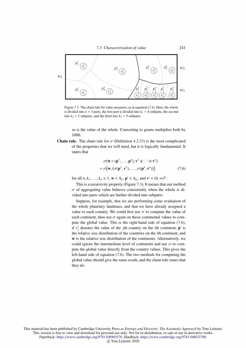
This material has been published by Cambridge University Press as Entropy and Diversity: The Axiomatic Approach by Tom Leinster.This version is free to view and download for personal use only. Not for re-distribution, re-sale or use in derivative works.
Paperback: https://www.cambridge.org/9781108965576. Hardback: https://www.cambridge.org/9781108832700.© Tom Leinster 2020
7.3 Characterization of value 241
w1
w2
w3
p11 v1
1n
p12 v1
2n
p13 v1
3n p1
4 v14n
p21 v2
1n p2
2 v22n
p31
v31n p3
2
v32n p3
3
v33np3
4
v34n p3
5
v35n
Figure 7.3 The chain rule for value measures, as in equation (7.6). Here, the wholeis divided into n = 3 parts, the first part is divided into k1 = 4 subparts, the secondinto k2 = 2 subparts, and the third into k3 = 5 subparts.
so is the value of the whole. Converting to grams multiplies both by1000.
Chain rule. The chain rule for σ (Definition 4.2.23) is the most complicatedof the properties that we will need, but it is logically fundamental. Itstates that
σ(w (p1, . . . ,pn), v1 ⊕ · · · ⊕ vn)
= σ(w,
(σ(p1, v1), . . . , σ(pn, vn)
))(7.6)
for all n, k1, . . . , kn ≥ 1, w ∈ ∆n, pi ∈ ∆ki , and vi ∈ (0,∞)ki .This is a recursivity property (Figure 7.3). It means that our method
σ of aggregating value behaves consistently when the whole is di-vided into parts which are further divided into subparts.
Suppose, for example, that we are performing some evaluation ofthe whole planetary landmass, and that we have already assigned avalue to each country. We could first use σ to compute the value ofeach continent, then use σ again on those continental values to com-pute the global value. This is the right-hand side of equation (7.6),if vi
j denotes the value of the jth country on the ith continent, pi isthe relative size distribution of the countries on the ith continent, andw is the relative size distribution of the continents. Alternatively, wecould ignore the intermediate level of continents and use σ to com-pute the global value directly from the country values. This gives theleft-hand side of equation (7.6). The two methods for computing theglobal value should give the same result, and the chain rule states thatthey do.

This material has been published by Cambridge University Press as Entropy and Diversity: The Axiomatic Approach by Tom Leinster.This version is free to view and download for personal use only. Not for re-distribution, re-sale or use in derivative works.
Paperback: https://www.cambridge.org/9781108965576. Hardback: https://www.cambridge.org/9781108832700.© Tom Leinster 2020
242 Value
We make two further definitions for value measures σ on (0,∞).
Definition 7.3.1 σ is continuous in positive probabilities if for each n ≥ 1and v ∈ (0,∞)n, the function
σ(−, v) : ∆n → (0,∞)p 7→ σ(p, v)
on the open simplex is continuous.
This condition only involves continuity in the sizes of the parts present, nottheir values. The restriction to the interior of the simplex means that we donot forbid value measures that make a sharp distinction between presence andabsence.
Definition 7.3.2 σ is an effective number if
σ(un, (1, . . . , 1)
)= n
for all n ≥ 1.
Assuming homogeneity, the effective number property is equivalent to
σ(un, (v, . . . , v)
)= nv (7.7)
for all n ≥ 1 and v ∈ (0,∞). That is, if we put together n parts of equal size andequal value, v, the result has value nv.
Remark 7.3.3 Let σ be an absence-invariant value measure. Then σ(p, v) isindependent of vi for i < supp(p). Indeed, writing supp(p) = i1, . . . , ik withi1 < · · · < ik, absence-invariance implies that
σ(p, v) = σ((pi1 , . . . , pik ), (vi1 , . . . , vik )
). (7.8)
So we can consistently extend the definition of σ(p, v) to pairs (p, v) where vi
need not be within the permissible range (0,∞), or even defined at all, wheni < supp(p). In that case, we define σ(p, v) to be the right-hand side of equa-tion (7.8). This convention is exactly analogous to the convention for meansintroduced in Remark 4.2.15, and to the usual convention for integrals of func-tions undefined on a set of measure zero.
We now prove that the properties listed above uniquely characterize the fam-ily of value measures (σq).
Theorem 7.3.4 Let(σ : ∆n × (0,∞)n → (0,∞)
)n≥1 be a sequence of functions.
The following are equivalent:

This material has been published by Cambridge University Press as Entropy and Diversity: The Axiomatic Approach by Tom Leinster.This version is free to view and download for personal use only. Not for re-distribution, re-sale or use in derivative works.
Paperback: https://www.cambridge.org/9781108965576. Hardback: https://www.cambridge.org/9781108832700.© Tom Leinster 2020
7.3 Characterization of value 243
i. σ is symmetric, absence-invariant, increasing, homogeneous, continuous inpositive probabilities and an effective number, and satisfies the chain rule;
ii. σ = σq for some q ∈ [−∞,∞].
Proof To prove that (ii) implies (i), let q ∈ [−∞,∞]. That σq is symmetric,absence-invariant, increasing, homogeneous, and continuous in positive prob-abilities follows from the definition
σq(p, v) = M1−q(p, v/p)
ofσq and the corresponding properties of M1−q (Lemmas 4.2.11, 4.2.19, 4.2.22and 4.2.6(i)). That σq is an effective number follows from the consistency ofM1−q, and the chain rule for σq follows from the chain rule for M1−q (Proposi-tion 4.2.24).
Conversely, assume that σ satisfies the conditions in (i). Define a sequenceof functions (
M : ∆n × (0,∞)n → (0,∞))n≥1
by
M(p, x) = σ(p,px)
(p ∈ ∆n, x ∈ (0,∞)n). Although it may be that (px)i = 0 for some i, in whichcase σ(p,px) is strictly speaking undefined, this can only happen when pi = 0;hence σ(p,px) can be interpreted according to the convention of Remark 7.3.3.
We will prove that M is a power mean. We do this by showing that M sat-isfies the hypotheses of Theorem 5.5.10: M is symmetric, absence-invariant,increasing, homogeneous, modular, and consistent. The first four follow fromthe corresponding properties of σ. It remains to prove that M is modular andconsistent.
For modularity, let w ∈ ∆n, pi ∈ ∆ki , and xi ∈ (0,∞)ki . Using the chain ruleand homogeneity properties of σ, we find that
M(w (p1, . . . ,pn), x1 ⊕ · · · ⊕ xn)
= σ(w (p1, . . . ,pn),w1p1x1 ⊕ · · · ⊕ wnpnxn)
= σ(w,
(σ(p1,w1p1x1), . . . , σ(
pn,wnpnxn)))= σ
(w,
(w1M(p1, x1), . . . ,wnM(pn, xn)
))= M
(w,
(M(p1, x1), . . . ,M(pn, xn)
)).
Hence M satisfies the chain rule, and is therefore modular.Proving that M is consistent is equivalent, by homogeneity, to showing that
σ(p,p) = 1

This material has been published by Cambridge University Press as Entropy and Diversity: The Axiomatic Approach by Tom Leinster.This version is free to view and download for personal use only. Not for re-distribution, re-sale or use in derivative works.
Paperback: https://www.cambridge.org/9781108965576. Hardback: https://www.cambridge.org/9781108832700.© Tom Leinster 2020
244 Value
for all n ≥ 1 and p ∈ ∆n. We do this in three steps.First suppose that the coordinates of p are positive and rational, so that p =
(k1/k, . . . , kn/k) for some positive integers ki summing to k. Then
uk = p (uk1 , . . . ,ukn ),
so by the chain rule for σ,
σ(uk, k ∗ 1) = σ(p,
(σ(uk1 , k1 ∗ 1), . . . , σ(ukn , kn ∗ 1)
)).
By the effective number property of σ, this means that
k = σ(p, (k1, . . . , kn)
).
Dividing through by k and using the homogeneity of σ gives 1 = σ(p,p), asrequired.
For the second step, let p be any point in ∆n. Let ε > 0. Sinceσ is continuousin positive probabilities, there is some δ > 0 such that for r ∈ ∆n,
‖p − r‖ < δ =⇒ |σ(p,p) − σ(r,p)| < ε/2, (7.9)
where ‖ · ‖ denotes Euclidean length. We can choose r ∈ ∆n with rationalcoordinates such that
‖p − r‖ < δ, maxi
pi
ri≤ 1 +
ε
2, min
i
pi
ri≥ 1 −
ε
2.
Since σ is increasing and homogeneous,
σ(r,p) ≤ σ(r,
(max
i
pi
ri
)r)
=
(max
i
pi
ri
)σ(r, r),
which by the first step gives
σ(r,p) ≤ maxi
pi
ri≤ 1 +
ε
2.
Similarly, σ(r,p) ≥ 1 − ε/2, so
|σ(r,p) − 1| ≤ ε/2.
This, together with (7.9) and the triangle inequality, implies that |σ(p,p)−1| <ε. But ε was arbitrary, so σ(p,p) = 1.
Third and finally, take any p ∈ ∆n. Write supp(p) = i1, . . . , ik with i1 <
· · · < ik, and write r = (pi1 , . . . , pik ) ∈ ∆k . Then
σ(p,p) = σ(r, r) = 1,
where the first equality holds for the reasons given in Remark 7.3.3, and thesecond follows from the second step above.
This completes the proof that M is consistent. We have now shown that M
This material has been published by Cambridge University Press as Entropy and Diversity: The Axiomatic Approach by Tom Leinster.This version is free to view and download for personal use only. Not for re-distribution, re-sale or use in derivative works.
Paperback: https://www.cambridge.org/9781108965576. Hardback: https://www.cambridge.org/9781108832700.© Tom Leinster 2020
7.4 Total characterization of the Hill numbers 245
satisfies the hypotheses of Theorem 5.5.10. By that theorem, M = M1−q forsome q ∈ [−∞,∞]. It follows that
σ(p, v) = M1−q(p, v/p) = σq(p, v)
for all n ≥ 1, p ∈ ∆n, and v ∈ (0,∞)n.
Remark 7.3.5 A similar characterization theorem can be proved for valuesin [0,∞) instead of (0,∞), using Theorem 5.5.11 on means on [0,∞). In thiscase, we have to strengthen the continuity requirement, also asking that σ(p, v)is continuous in v for each fixed p.
Theorem 7.3.4 can be translated into a characterization theorem for eitherthe Renyi relative entropies or the q-logarithmic relative entropies, using theobservations in Section 7.2. This translation exercise is left to the reader.
7.4 Total characterization of the Hill numbers
The axiomatic approach to diversity measurement is to specify mathematicalproperties that we want the concept of diversity to possess, then to prove atheorem classifying all the diversity measures with the specified properties.
Here we do this for the simple but very commonplace model of a commu-nity as its relative abundance distribution p = (p1, . . . , pn). We prove that anymeasure p 7→ D(p) satisfying a handful of intuitive properties must be oneof the Hill numbers Dq. To do this, we use the characterization theorem forvalue measures (Theorem 7.3.4). The strategy is to construct from our hypo-thetical diversity measure D a value measure σ, apply Theorem 7.3.4 to showthat σ = σq for some q, and deduce from this that D = Dq.
This is the second characterization theorem for the Hill numbers that wehave proved, and it is more powerful than the first (Theorem 4.5.1), in thesense that the hypotheses are simpler and have more direct ecological explana-tions. Another difference is that the previous theorem fixed a parameter valueq, whereas the one below characterizes Dq for all q simultaneously. Furtherdiscussion of the differences can be found at the end of the introduction to thischapter.
Consider, then, a sequence of functions(D : ∆n → (0,∞)
)n≥1,
intended to measure the diversity D(p) of any community of n species withrelative abundances p = (p1, . . . , pn). What properties would we expect D topossess?

This material has been published by Cambridge University Press as Entropy and Diversity: The Axiomatic Approach by Tom Leinster.This version is free to view and download for personal use only. Not for re-distribution, re-sale or use in derivative works.
Paperback: https://www.cambridge.org/9781108965576. Hardback: https://www.cambridge.org/9781108832700.© Tom Leinster 2020
246 Value
We already discussed some desirable properties in Section 4.4, arguing thatany reasonable diversity measure D ought to be symmetric, absence-invariant,and continuous in positive probabilities, and that it should obey the replicationprinciple. To fix the scale on which we are working, we also ask that a commu-nity consisting of only one species has diversity 1. Formally, D is normalizedif D(u1) = 1.
We impose one further condition on our hypothetical diversity measure.Consider a pair of islands, perhaps with different population sizes, with nospecies in common. Replace the population of the first island by a populationof the same abundance but greater or equal diversity, still sharing no specieswith the second island. Then the diversity of the two-island community shouldbe greater than or equal to what it was originally.
More generally, consider a group of several islands, perhaps with differentpopulation sizes, with no species shared between islands. Replace the popula-tion of each island by a population of the same abundance but greater or equaldiversity, and still with no shared species between islands. Then the diversityof the whole island group should be greater than or equal to what it was orig-inally. Although this condition is superficially stronger than the special casedescribed in the previous paragraph, it is equivalent by induction. We formal-ize it as follows.
Definition 7.4.1 A sequence of functions(D : ∆n → (0,∞)
)n≥1 is modular-
monotone if
D(pi) ≤ D(pi) for all i ∈ 1, . . . , n
=⇒ D(w (p1, . . . ,pn)
)≤ D
(w (p1, . . . , pn)
)for all n, ki, ki ≥ 1 and w ∈ ∆n, pi ∈ ∆ki and pi ∈ ∆ki
.
For comparison, recall that by definition, D is modular if and only if
D(pi) = D
(pi) for all i ∈ 1, . . . , n
=⇒ D(w (p1, . . . ,pn)
)= D
(w (p1, . . . , pn)
)(Definition 4.4.14). Modular-monotonicity implies modularity (Lemma 7.4.4),and like modularity, it is a basic requirement for a diversity measure.
Example 7.4.2 Let q ∈ [−∞,∞]. The Hill number Dq is modular-monotone,since by the chain rule for Dq (Proposition 4.4.10),
Dq(w (p1, . . . ,pn)
)= M1−q
(w,
(Dq(p1)/w1, . . . ,Dq(pn)/wn
)),
and the power mean M1−q is increasing.

This material has been published by Cambridge University Press as Entropy and Diversity: The Axiomatic Approach by Tom Leinster.This version is free to view and download for personal use only. Not for re-distribution, re-sale or use in derivative works.
Paperback: https://www.cambridge.org/9781108965576. Hardback: https://www.cambridge.org/9781108832700.© Tom Leinster 2020
7.4 Total characterization of the Hill numbers 247
We will prove:
Theorem 7.4.3 Let(D : ∆n → (0,∞)
)n≥1 be a sequence of functions. The fol-
lowing are equivalent:
i. D is symmetric, absence-invariant, continuous in positive probabilities,normalized and modular-monotone, and satisfies the replication principle;
ii. D = Dq for some q ∈ [−∞,∞].
The rest of this section is devoted to the proof, and to a refinement of thetheorem that excludes negative values of q. We have already shown that (ii)implies (i), so it remains to prove the converse.
For the rest of this section, let(D : ∆n → (0,∞)
)n≥1
be a sequence of functions satisfying the six conditions in Theorem 7.4.3(i).We begin our proof by proving that the assumed properties of D imply some
of the other desirable properties discussed in Section 4.4.
Lemma 7.4.4 D is an effective number and modular.
Proof For the effective number property, we have
D(un) = D(un ⊗ u1) = nD(u1) = n
for each n ≥ 1, by replication and normalization.Modularity follows from modular-monotonicity, since in the notation of
Definition 4.4.14, if D(pi) = D(pi) then D(pi) ≤ D(pi) ≤ D(pi).
The next few results establish that D is multiplicative. This is harder. Firstwe prove the weaker statement that D(p ⊗ r) depends only on D(p) and D(r).
Lemma 7.4.5 Let p ∈ ∆m, p′ ∈ ∆m′ , r ∈ ∆n, and r′ ∈ ∆n′ . Then
D(p) = D(p′), D(r) = D(r′) =⇒ D(p ⊗ r) = D(p′ ⊗ r′).
Proof Suppose that D(p) = D(p′) and D(r) = D(r′). By definition of ⊗ andmodularity,
D(p ⊗ r) = D(p (r, . . . , r)
)= D
(p (r′, . . . , r′)
)= D(p ⊗ r′).
By symmetry of D, the order of the factors in the tensor product is irrelevant,so D(p ⊗ r′) = D(p′ ⊗ r′) by the same argument. The result follows.

This material has been published by Cambridge University Press as Entropy and Diversity: The Axiomatic Approach by Tom Leinster.This version is free to view and download for personal use only. Not for re-distribution, re-sale or use in derivative works.
Paperback: https://www.cambridge.org/9781108965576. Hardback: https://www.cambridge.org/9781108832700.© Tom Leinster 2020
248 Value
∆n
p1p2
p3 . . .p′
p
(0,∞)D(p1)∈ Q
D(p2)∈ Q
D(p3)∈ Q
· · ·
D(p′)= D(p)
Figure 7.4 Schematic illustration of Lemma 7.4.6.
As the next step in showing that D is multiplicative, we prove a technicallemma (Figure 7.4).
Lemma 7.4.6 Let n ≥ 1 and p ∈ ∆n. Then there exists a sequence (p j)∞j=1 in∆n converging to a point p′ ∈ ∆n, such that D(p j) is rational for all j andD(p′) = D(p).
Proof We can choose a continuous map γ : [0, 1] → ∆n such that γ(0) =
un and γ(1) = p. (For example, take γ(t) = (1 − t)un + tp.) By continuityin positive probabilities, Dγ[0, 1] is connected and is therefore a subintervalof (0,∞). It contains D(γ(0)), which by the effective number property is n,and also contains D(γ(1)) = D(p). Hence Dγ[0, 1] contains all real numbersbetween n and D(p). Either D(p) = n or D(p) , n, and in either case, there issome sequence (d j)∞j=1 of rational numbers in Dγ[0, 1] that converges to D(p)and is either increasing or decreasing. (In the case D(p) = n, we can simplytake d j = n for all j.)
Since d1 ∈ Dγ[0, 1], we can choose t1 ∈ [0, 1] such that D(γ(t1)) = d1. Thenby continuity in positive probabilities, Dγ[t1, 1] is an interval containing d1 andD(γ(1)) = D(p). But (d j) is an increasing or decreasing sequence convergingto D(p), so the interval Dγ[t1, 1] also contains d2. Hence we can choose t2 ∈[t1, 1] such that D(γ(t2)) = d2. Continuing in this way, we obtain an increasingsequence (t j)∞j=1 in [0, 1] with D(γ(t j)) = d j for all j ≥ 1.
Put p j = γ(t j) ∈ ∆n for each j ≥ 1. Then D(p j) = d j ∈ Q for all j. Also putt = sup j t j ∈ [0, 1] and p′ = γ(t) ∈ ∆n. Then t j → t as j→ ∞, so
p j = γ(t j)→ γ(t) = p′
as j → ∞. Since D is continuous in positive probabilities, this implies that

This material has been published by Cambridge University Press as Entropy and Diversity: The Axiomatic Approach by Tom Leinster.This version is free to view and download for personal use only. Not for re-distribution, re-sale or use in derivative works.
Paperback: https://www.cambridge.org/9781108965576. Hardback: https://www.cambridge.org/9781108832700.© Tom Leinster 2020
7.4 Total characterization of the Hill numbers 249
D(p j) → D(p′) as j → ∞. But also D(p j) = d j → D(p) as j → ∞, bydefinition of the sequence (d j). Hence D(p′) = D(p), as required.
Lemma 7.4.7 D is multiplicative.
Proof Let p ∈ ∆m and r ∈ ∆n. We have to show that D(p ⊗ r) = D(p)D(r).First suppose that D(p) is rational, say D(p) = a/b for positive integers a
and b. Since D is an effective number, bD(p) = D(ua). Hence by replication,
D(ub ⊗ p) = D(ua). (7.10)
Now
bD(p ⊗ r) = D(ub ⊗ p ⊗ r) (7.11)
= D(ua ⊗ r) (7.12)
= aD(r), (7.13)
where (7.11) and (7.13) follow from the replication principle for D, and (7.12)follows from (7.10) and Lemma 7.4.5. Hence
D(p ⊗ r) = (a/b)D(r) = D(p)D(r),
as required.Next we prove that D(p⊗ r) = D(p)D(r) in the case that p ∈ ∆m and r ∈ ∆n.
Choose a sequence (p j) in ∆m converging to p′ ∈ ∆m as in Lemma 7.4.6. Bythe previous paragraph,
D(p j ⊗ r) = D(p j)D(r) (7.14)
for all j ≥ 1. Now p j ⊗ r ∈ ∆mn for all j, and p j ⊗ r→ p′ ⊗ r as j→ ∞. Hence,taking the limit as j → ∞ in equation (7.14) and using continuity in positiveprobabilities,
D(p′ ⊗ r) = D(p′)D(r).
But D(p′) = D(p), so by Lemma 7.4.5,
D(p ⊗ r) = D(p)D(r),
as required.Finally, we prove multiplicativity for an arbitrary p ∈ ∆m and r ∈ ∆n. By
symmetry, we may suppose that p = (p1, . . . , pm′ , 0, . . . , 0) with p1, . . . , pm′ >
0. Write p′ = (p1, . . . , pm′ ) ∈ ∆m′ , and similarly r′ ∈ ∆n′ . By the previousparagraph, D(p′ ⊗ r′) = D(p′)D(r′). On the other hand, by absence-invariance,D(p′) = D(p) and D(r′) = D(r). Hence by Lemma 7.4.5, D(p⊗r) = D(p)D(r),completing the proof.

This material has been published by Cambridge University Press as Entropy and Diversity: The Axiomatic Approach by Tom Leinster.This version is free to view and download for personal use only. Not for re-distribution, re-sale or use in derivative works.
Paperback: https://www.cambridge.org/9781108965576. Hardback: https://www.cambridge.org/9781108832700.© Tom Leinster 2020
250 Value
The plan for the rest of the proof of Theorem 7.4.3 is as follows. We wish toshow that D = Dq for some q. We know that the Hill number Dq satisfies thechain rule
Dq(w (p1, . . . ,pn)
)= σq
(w,
(Dq(p1), . . . ,Dq(pn)
))(Example 7.1.8). Our diversity measure D is modular, which means that D
(w
(p1, . . . ,pn))
is some function of w and D(p1), . . . ,D(pn). We will therefore beable to define a function σ by
D(w (p1, . . . ,pn)
)= σ
(w,
(D(p1), . . . ,D(pn)
)). (7.15)
Roughly speaking, we then show that the assumed good properties of the diver-sity measure D imply good properties of σ, deduce from our earlier character-ization of value measures that σ = σq for some q, and conclude that D = Dq.
There is a subtlety. In order to use the characterization of value measures(Theorem 7.3.4), we need σ to be defined on all pairs σ(p, v) with p ∈ ∆n andv ∈ (0,∞)n, whereas equation (7.15) only defines σ(p, v) on vectors v whosecoordinates vi can be expressed as values of the diversity measure D. And itmay happen that some elements of (0,∞) do not arise as values of D. Indeed,if D = Dq then Dq(r) ≥ 1 for all distributions r.
For this reason, we now analyse the set of real numbers that arise as diversi-ties D(p). Write
im D =
∞⋃n=1
D∆n ⊆ (0,∞).
The case of the Hill numbers shows that the situation is not entirely simple:
Example 7.4.8 For q ∈ [−∞,∞], the Hill number Dq has image
im Dq =
[1,∞) if q > 0,
1, 2, 3, . . . if q = 0,
1 ∪ [2,∞) if q < 0.
(7.16)
The statement for q > 0 follows from the facts that Dq(p) ≥ 1 for allp (Lemma 4.4.3(i)), Dq is an effective number (equation (4.25)), and Dq
is continuous (Lemma 4.4.6(ii)). For q = 0, the result is immediate, sinceD0(p) = |supp(p)|.
Now let q < 0. Since diversity profiles are decreasing (Proposition 4.4.1),
Dq(p) ≥ |supp(p)|
for all p. If |supp(p)| = 1 then p = (0, . . . , 0, 1, 0, . . . , 0) and so Dq(p) = 1.Otherwise, |supp(p)| ≥ 2, so Dq(p) ∈ [2,∞). Hence im Dq ⊆ 1 ∪ [2,∞). To
This material has been published by Cambridge University Press as Entropy and Diversity: The Axiomatic Approach by Tom Leinster.This version is free to view and download for personal use only. Not for re-distribution, re-sale or use in derivative works.
Paperback: https://www.cambridge.org/9781108965576. Hardback: https://www.cambridge.org/9781108832700.© Tom Leinster 2020
7.4 Total characterization of the Hill numbers 251
prove the opposite inclusion, first note that both 1 = Dq(u1) and 2 = Dq(u2)belong to im Dq. An elementary calculation shows that
Dq(t, 1 − t)→ ∞ as t → 0+.
Since Dq : ∆2 → (0,∞) is continuous (Lemma 4.4.6(i)), Dq∆2 is an intervalthat contains 2 and is unbounded above. Hence Dq∆2 ⊇ [2,∞), completing theproof of the last clause of equation (7.16).
Lemma 7.4.9 im D is closed under multiplication.
Proof This follows from the multiplicativity of D (Lemma 7.4.7).
Lemma 7.4.10 Suppose that D , D0. Then im D ⊇ [L,∞) for some L > 0.
Proof If D∆n is a one-element set for each n ≥ 1 then by the effective numberproperty, D∆n = n for each n. Hence by absence-invariance, D = D0, acontradiction.
We can therefore choose n ≥ 1 such that D∆n has more than one element,which by continuity in positive probabilities implies that D∆n is a nontrivialinterval. Since D is an effective number, this interval contains n. Now n , 1(since D∆1 is trivial), so n ≥ 2, so im D ∩ [1,∞) contains a nontrivial interval.Since both im D and [1,∞) are closed under multiplication, so is im D∩[1,∞).
It is now enough to prove that any subset B of [1,∞) that is closed undermultiplication and contains a nontrivial interval must contain [L,∞) for someL ≥ 1. Indeed, since B contains a nontrivial interval, B ⊇ [b, b1+1/r] for somereal b > 1 and positive integer r. Since B is closed under multiplication, it isclosed under positive integer powers, so for every integer m ≥ r,
B ⊇ [bm, bm+m/r] ⊇ [bm, bm+1].
Hence
B ⊇⋃m≥r
[bm, bm+1] = [br,∞),
using b > 1 in the last step.
We now construct from D a value measure σ. The construction proceeds intwo steps. First, since D is modular, we can consistently define a sequence offunctions (
ρ : ∆n × (im D)n → im D)n≥1
by
ρ(w,
(D(p1), . . . ,D(pn)
))= D
(w (p1, . . . ,pn)
)

This material has been published by Cambridge University Press as Entropy and Diversity: The Axiomatic Approach by Tom Leinster.This version is free to view and download for personal use only. Not for re-distribution, re-sale or use in derivative works.
Paperback: https://www.cambridge.org/9781108965576. Hardback: https://www.cambridge.org/9781108832700.© Tom Leinster 2020
252 Value
for all n, k1, . . . , kn ≥ 1, w ∈ ∆n and pi ∈ ∆ki . Second, we extend ρ to a sequenceof functions defined on not just ∆n × (im D)n, but the whole of ∆n × (0,∞)n:
Lemma 7.4.11 Suppose that D , D0. Then there is a unique homogeneoussequence of functions (
σ : ∆n × (0,∞)n → (0,∞))n≥1
such that
σ(w,
(D(p1), . . . ,D(pn)
))= D
(w (p1, . . . ,pn)
)for all n, k1, . . . , kn ≥ 1, w ∈ ∆n, and pi ∈ ∆ki .
In brief, there is a unique homogeneous extension of ρ from im D to (0,∞).
Proof We begin by establishing a homogeneity property of ρ:
ρ(w, cx) = cρ(w, x) (7.17)
for all w ∈ ∆n, x ∈ (im D)n, and c ∈ im D. (The left-hand side is well-definedsince im D is closed under multiplication, by Lemma 7.4.9.) To prove this, foreach i ∈ 1, . . . , n, choose pi ∈ ∆ki such that D(pi) = xi, and choose r ∈ ∆m
such that D(r) = c. Then
ρ(w, cx) = ρ(w,
(D(p1)D(r), . . . ,D(pn)D(r)
))(7.18)
= ρ(w,
(D(p1 ⊗ r), . . . ,D(pn ⊗ r)
))(7.19)
= D(w (p1 ⊗ r, . . . ,pn ⊗ r)
)(7.20)
= D((
w (p1, . . . ,pn))⊗ r
)(7.21)
= D(w (p1, . . . ,pn)
)D(r) (7.22)
= cρ(w, x), (7.23)
where equation (7.18) is by definition of pi and r, equations (7.19) and (7.22)are by multiplicativity of D (Lemma 7.4.7), equations (7.20) and (7.23) are bydefinition of ρ, and (7.21) is by associativity of composition of distributions(Remark 2.1.8). This proves the claimed homogeneity equation (7.17).
We now prove the uniqueness and existence stated in the lemma.
Uniqueness Let p ∈ ∆n and v ∈ (0,∞)n. By Lemma 7.4.10, im D containsall sufficiently large real numbers, so we can choose c ∈ (0,∞) such that cv ∈(im D)n. Then ρ(p, cv) is defined, and any sequence of homogeneous functionsσ extending ρ satisfies
σ(p, v) = 1cρ(p, cv).
This proves uniqueness.
This material has been published by Cambridge University Press as Entropy and Diversity: The Axiomatic Approach by Tom Leinster.This version is free to view and download for personal use only. Not for re-distribution, re-sale or use in derivative works.
Paperback: https://www.cambridge.org/9781108965576. Hardback: https://www.cambridge.org/9781108832700.© Tom Leinster 2020
7.4 Total characterization of the Hill numbers 253
Existence First I claim that for all p ∈ ∆n, v ∈ (0,∞)n, and c, d ∈ (0,∞) suchthat cv, dv ∈ (im D)n,
1cρ(p, cv) = 1
dρ(p, dv). (7.24)
Indeed, since im D contains all sufficiently large real numbers, we can choosea > 0 such that ac, ad ∈ im D. Then
ad · ρ(p, cv) = ρ(p, acdv)
by the homogeneity property (7.17) of ρ. Similarly,
ac · ρ(p, dv) = ρ(p, acdv).
Combining the last two equations gives equation (7.24), as claimed.It follows that there is a unique sequence of functions(
σ : ∆n × (0,∞)n → (0,∞))n≥1
satisfying
σ(p, v) = 1cρ(p, cv) (7.25)
whenever p ∈ ∆n, v ∈ (0,∞)n and c ∈ (0,∞) with cv ∈ (im D)n.It remains to prove that σ is homogeneous. Let p ∈ ∆n, v ∈ (0,∞)n, and
a ∈ (0,∞); we must show that
σ(p, av) = aσ(p, v). (7.26)
Choose d ∈ (0,∞) such that adv, dv ∈ (im D)n. By the claim just proved,
1adρ(p, adv) = 1
dρ(p, dv),
or equivalently,1dρ(p, d · av) = a · 1
dρ(p, dv).
But by the defining property (7.25) of σ, this is exactly the desired equa-tion (7.26).
Example 7.4.12 Consider the case D = Dq. We have
σq
(w,
(Dq(p1), . . . ,Dq(pn)
))= Dq
(w (p1, . . . ,pn)
)for all w and pi, by Example 7.1.8. Moreover, σq is homogeneous. Hence bythe uniqueness part of Lemma 7.4.11, σ = σq.
We have now constructed from our diversity measure D a value measure σ.From our standing assumption that D has certain good properties, it followsthat σ has good properties too:
This material has been published by Cambridge University Press as Entropy and Diversity: The Axiomatic Approach by Tom Leinster.This version is free to view and download for personal use only. Not for re-distribution, re-sale or use in derivative works.
Paperback: https://www.cambridge.org/9781108965576. Hardback: https://www.cambridge.org/9781108832700.© Tom Leinster 2020
254 Value
Lemma 7.4.13 Suppose that D , D0. Then σ is symmetric, absence-invariant, increasing, homogeneous, continuous in positive probabilities andan effective number, and satisfies the chain rule.
Proof The symmetry, absence-invariance and effective number properties ofD imply the corresponding properties of σ. The modular-monotonicity of Dimplies that ρ, hence σ, is increasing. Homogeneity is one of the defining prop-erties of σ (Lemma 7.4.11). It remains to prove continuity in positive proba-bilities and the chain rule.
To prove that σ is continuous in positive probabilities, let v ∈ (0,∞)n; wewish to prove that
σ(−, v) : ∆n → (0,∞)
is continuous. Choose c ∈ (0,∞) such that cv ∈ (im D)n. Then σ(−, v) =1cρ(−, cv). It therefore suffices to prove that
ρ(−, x) : ∆n → (0,∞)
is continuous for every x ∈ (im D)n. For each i ∈ 1, . . . , n, choose pi ∈ ∆ki
such that xi = D(pi). By absence-invariance, we may assume that each pi hasfull support. For all w ∈ ∆n, we have
ρ(w, x) = D(w (p1, . . . ,pn)
),
and if w has full support then so does w (p1, . . . ,pn). Thus, the restriction ofρ(−, x) to ∆n is the composite of the continuous maps
∆n// ∆k1+···+kn
D // (0,∞)
w // w (p1, . . . ,pn).
It is therefore continuous, as claimed.To prove that σ satisfies the chain rule, we first prove a chain rule for ρ:
ρ(w (p1, . . . ,pn), x1 ⊕ · · · ⊕ xn) = ρ
(w,
(ρ(p1, x1), . . . , ρ(pn, xn)
))(7.27)
for all w ∈ ∆n, pi ∈ ∆ki , and xi ∈ (im D)ki . To see this, begin by choosing foreach i ∈ 1, . . . , n and j ∈ 1, . . . , ki a probability distribution ri
j such thatD(ri
j) = xij. Then by definition of ρ, the left-hand side of equation (7.27) is
equal to
D((
w (p1, . . . ,pn))(r1
1, . . . , r1k1, . . . , rn
1, . . . , rnkn
)).
By associativity of composition of distributions (Remark 2.1.8), this is equalto
D(w
(p1
(r1
1, . . . , r1k1
), . . . , pn
(rn
1, . . . , rnkn
))).

This material has been published by Cambridge University Press as Entropy and Diversity: The Axiomatic Approach by Tom Leinster.This version is free to view and download for personal use only. Not for re-distribution, re-sale or use in derivative works.
Paperback: https://www.cambridge.org/9781108965576. Hardback: https://www.cambridge.org/9781108832700.© Tom Leinster 2020
7.4 Total characterization of the Hill numbers 255
By definition of ρ, this in turn is equal to
ρ(w,
(D(p1
(r1
1, . . . , r1k1
)), . . . , D
(pn
(rn
1, . . . , rnkn
)))),
which by definition of ρ again is equal to the right-hand side of (7.27). Thisproves the claimed chain rule (7.27) for ρ.
We now want to prove the chain rule for σ:
σ(w (p1, . . . ,pn), v1 ⊕ · · · ⊕ vn) = σ
(w,
(σ(p1, v1), . . . , σ(pn, vn)
))for all w ∈ ∆n, pi ∈ ∆ki , and vi ∈ (0,∞)ki . We may choose c ∈ (0,∞) such thatcvi
j ∈ im D for all i, j. Then by definition of σ and the chain rule (7.27) for ρ,
σ(w (p1, . . . ,pn), v1 ⊕ · · · ⊕ vn) = 1
cρ(w (p1, . . . ,pn), cv1 ⊕ · · · ⊕ cvn)
= 1cρ
(w,
(ρ(p1, cv1), . . . , ρ(pn, cvn)
))= 1
cρ(w,
(cσ(p1, v1), . . . , cσ(pn, vn)
))= σ
(w,
(σ(p1, v1), . . . , σ(pn, vn)
)),
as required.
We are now ready to prove that when a community is modelled as a proba-bility distribution, the Hill numbers are the only sensible measures of diversity.
Proof of Theorem 7.4.3 We have to show that D = Dq for some q ∈ [−∞,∞].If D = D0, this is immediate. Otherwise, by Lemma 7.4.13, σ is a value mea-sure satisfying the hypotheses of Theorem 7.3.4. By that theorem, σ = σq forsome q ∈ [−∞,∞]. Let p ∈ ∆n. Then
D(p) = D(p (u1, . . . ,u1︸ ︷︷ ︸
n
))
= ρ(p,
(D(u1), . . . ,D(u1)
))(7.28)
= ρ(p, (1, . . . , 1)
)(7.29)
= σq(p, (1, . . . , 1)
)(7.30)
= Dq(p), (7.31)
where equation (7.28) is by definition of ρ, equation (7.29) holds because Dis normalized, equation (7.30) holds because σ extends ρ and σ = σq, andequation (7.31) is from Example 7.1.6. Hence D = Dq.
The theorem axiomatically characterizes the whole family (σq)q∈[−∞,∞] ofHill numbers. But as argued in Remark 4.4.4(ii), Dq probably does not deserveto be called a measure of diversity when q is negative. We may therefore wish
This material has been published by Cambridge University Press as Entropy and Diversity: The Axiomatic Approach by Tom Leinster.This version is free to view and download for personal use only. Not for re-distribution, re-sale or use in derivative works.
Paperback: https://www.cambridge.org/9781108965576. Hardback: https://www.cambridge.org/9781108832700.© Tom Leinster 2020
256 Value
to characterize the Hill numbers Dq for which q ≥ 0, and the following resultachieves this.
Lemma 7.4.14 Let q ∈ [−∞,∞]. The following are equivalent:
i. Dq(p) ≤ Dq(un) for all n ≥ 1 and p ∈ ∆n;ii. Dq(p) ≤ 2 for all p ∈ ∆2;
iii. q ∈ [0,∞].
Proof (i) implies (ii) trivially, (ii) implies (iii) by Remark 4.4.4(ii), and (iii)implies (i) by Lemma 4.4.3(ii).
Remark 7.4.15 Our characterization theorem for the Hill numbers can easilybe translated into a characterization theorem for the Renyi or q-logarithmicentropies, using the transformations of Section 7.2. However, the hypothesesof Theorem 7.4.3 are particularly natural in the context of diversity.
When translated into terms of q-logarithmic entropy, Theorem 7.4.3 is ofthe same general type as a result of Forte and Ng [107] (also stated as Theo-rem 6.3.12 of Aczel and Daroczy [3]). Apart from some differences in hypothe-ses, Forte and Ng’s characterization excludes the case q = 0, which from thepoint of view of diversity measurement is a serious drawback: the Hill numberD0 is species richness, the most common diversity measure of all.
This material has been published by Cambridge University Press as Entropy and Diversity: The Axiomatic Approach by Tom Leinster.This version is free to view and download for personal use only. Not for re-distribution, re-sale or use in derivative works.
Paperback: https://www.cambridge.org/9781108965576. Hardback: https://www.cambridge.org/9781108832700.© Tom Leinster 2020
8
Mutual information and metacommunities
From the viewpoint of information theory, there is a conspicuous omissionfrom this text so far. Given a random variable X taking values in a finite set,we have a measure of the information associated with X: its entropy H(X).But suppose that we are also given another random variable Y , not necessarilyindependent of X, taking values in another finite set. If we know the value ofX, how much information does that give us about the value of Y?
For instance, Y might be a function of X, in which case knowing the valueof X gives complete information about Y . Or, at the other extreme, X and Ymight be independent, in which case knowing the value of X tells us nothingabout Y . We would like to quantify the dependence between the two variables.The covariance and correlation coefficients will not do, since they are usuallyonly defined for random variables taking values in Rn; and while they can bedefined in greater generality, there is no definition for an arbitrary pair of finitesets.
From the viewpoint of diversity measurement, there is also something miss-ing. We know how to quantify the diversity of a single community. But whenwe have several associated or adjacent communities – for instance, the gutmicrobiomes of healthy and unhealthy adults, or the aquatic life in areas ofdifferent salinity near the mouth of a river – some natural questions presentthemselves. How much variation is there between the communities? Whichcontribute most to the overall diversity? Which are most or least typical in thecontext of the system as a whole? The diversity measures discussed so far giveno answers to such questions.
We will see that these two problems, one information-theoretic and one eco-logical, have the same solution.
Our starting point is the classical information-theoretic concept of mutualinformation (a measure of the dependence between two random variables) andthe closely related concepts of conditional and joint entropy. These are in-
257

This material has been published by Cambridge University Press as Entropy and Diversity: The Axiomatic Approach by Tom Leinster.This version is free to view and download for personal use only. Not for re-distribution, re-sale or use in derivative works.
Paperback: https://www.cambridge.org/9781108965576. Hardback: https://www.cambridge.org/9781108832700.© Tom Leinster 2020
258 Mutual information and metacommunities
troduced in Section 8.1. Then we take exponentials of all these quantities,which produces a suite of meaningful measures of an ecological metacom-munity (large community) divided into smaller subcommunities. The two ran-dom variables in play here correspond to a choice of species and a choice ofsubcommunity. Some of the measures reflect features of individual subcom-munities (Section 8.2), while others encapsulate information about the entiremetacommunity (Section 8.3). We establish the many good logical propertiesof these measures in Section 8.4.
All of the entropies and diversities in this chapter can be reduced to relativeentropy (Section 8.5). In the diversity case, they are also usefully expressed interms of value, in the sense of Chapter 7. Reducing the various metacommunityand subcommunity measures to one single concept provides new insights intotheir ecological meaning.
The diversity measures treated in this chapter are a very special case of thoseintroduced in work of Reeve et al. [290]. In the terminology of Chapter 6, itis the case q = 1 (no deformation) and Z = I (no inter-species similarity).The framework of Reeve et al. allows a general q (variable emphasis on rare orcommon species) and a general Z (to model the varying similarities betweenspecies). Section 8.6 is a sketch of the development for a general q, the detailsof which lie outside the scope of this book.
8.1 Joint entropy, conditional entropy and mutualinformation
Shannon entropy H assigns a real number H(p) to each probability distributionp, but information theory also associates several quantities with any pair ofprobability distributions. To organize them, it is helpful to distinguish betweentwo types of quantity: those defined for a pair of distributions on the same set,and those defined for a pair of distributions on potentially different sets.
We have already met two quantities of the first type: the relative entropyH(p ‖ r) and cross entropy H×(p ‖ r) of two distributions p and r on the samefinite set (Chapter 3).
We now introduce the standard information-theoretic quantities of the sec-ond type. The material in this section is all classical, and can be found in textssuch as Cover and Thomas ([69], Chapter 2) and MacKay ([236], Chapter 8).As usual, we only consider probability distributions on finite sets. But it isconvenient to switch from the language of probability distributions to that ofrandom variables.
So, for the rest of this section, we consider a random variable X taking
This material has been published by Cambridge University Press as Entropy and Diversity: The Axiomatic Approach by Tom Leinster.This version is free to view and download for personal use only. Not for re-distribution, re-sale or use in derivative works.
Paperback: https://www.cambridge.org/9781108965576. Hardback: https://www.cambridge.org/9781108832700.© Tom Leinster 2020
8.1 Joint entropy, conditional entropy and mutual information 259
values in a finite set X, and another random variable Y taking values in a finiteset Y. Assuming that X and Y have the same sample space, we also have therandom variable (X,Y), which takes values in X ×Y.
Given x ∈ X and y ∈ Y, we write Pr((X,Y) = (x, y)) as Pr(X = x,Y = y).We usually abbreviate Pr(X = x) as Pr(x), etc. Thus, by definition, X and Y areindependent if and only if
Pr(x, y) = Pr(x) Pr(y)
for all x ∈ X and y ∈ Y. The conditional probability of x given y is
Pr(x | y) =Pr(x, y)Pr(y)
,
and is defined as long as Pr(y) > 0.The Shannon entropy of the random variable X is the Shannon entropy of
its distribution:
H(X) =∑
x : Pr(x)>0
Pr(x) log1
Pr(x).
Here and below, the variable x in summations is assumed to run over the set Xunless indicated otherwise, and similarly for y in Y.
Joint entropy
The general definition of the entropy of a random variable can be applied tothe random variable (X,Y), giving
H(X,Y) =∑
x,y : Pr(x,y)>0
Pr(x, y) log1
Pr(x, y),
the joint entropy of X and Y .
Examples 8.1.1 i. Suppose that X and Y are independent. If X has distribu-tion p and Y has distribution r then (X,Y) has distribution p ⊗ r, so
H(X,Y) = H(X) + H(Y)
by Corollary 2.2.10.ii. Suppose that Y is a one-element set. Then the distribution of Y is uniquely
determined, H(Y) = 0, and H(X,Y) = H(X).iii. Suppose that X = Y and X = Y . Then H(X,Y) = H(X) = H(Y).iv. Generalizing the last two examples, let us say that Y is determined by X
if for all x ∈ X such that Pr(x) > 0, there is a unique y ∈ Y such that
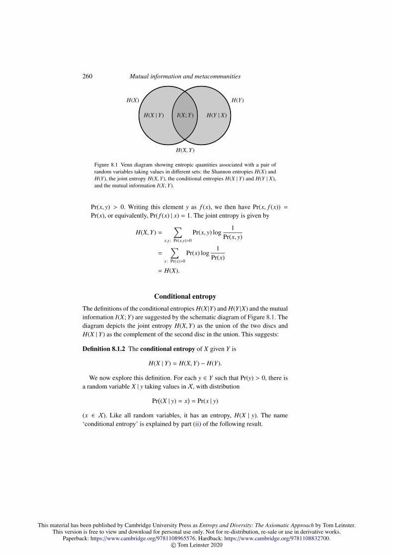
This material has been published by Cambridge University Press as Entropy and Diversity: The Axiomatic Approach by Tom Leinster.This version is free to view and download for personal use only. Not for re-distribution, re-sale or use in derivative works.
Paperback: https://www.cambridge.org/9781108965576. Hardback: https://www.cambridge.org/9781108832700.© Tom Leinster 2020
260 Mutual information and metacommunities
H(X,Y)
H(X) H(Y)
H(X | Y) I(X; Y) H(Y | X)
Figure 8.1 Venn diagram showing entropic quantities associated with a pair ofrandom variables taking values in different sets: the Shannon entropies H(X) andH(Y), the joint entropy H(X,Y), the conditional entropies H(X | Y) and H(Y | X),and the mutual information I(X; Y).
Pr(x, y) > 0. Writing this element y as f (x), we then have Pr(x, f (x)) =
Pr(x), or equivalently, Pr( f (x) | x) = 1. The joint entropy is given by
H(X,Y) =∑
x,y : Pr(x,y)>0
Pr(x, y) log1
Pr(x, y)
=∑
x : Pr(x)>0
Pr(x) log1
Pr(x)
= H(X).
Conditional entropy
The definitions of the conditional entropies H(X |Y) and H(Y |X) and the mutualinformation I(X; Y) are suggested by the schematic diagram of Figure 8.1. Thediagram depicts the joint entropy H(X,Y) as the union of the two discs andH(X | Y) as the complement of the second disc in the union. This suggests:
Definition 8.1.2 The conditional entropy of X given Y is
H(X | Y) = H(X,Y) − H(Y).
We now explore this definition. For each y ∈ Y such that Pr(y) > 0, there isa random variable X | y taking values in X, with distribution
Pr((X | y) = x
)= Pr(x | y)
(x ∈ X). Like all random variables, it has an entropy, H(X | y). The name‘conditional entropy’ is explained by part (ii) of the following result.
This material has been published by Cambridge University Press as Entropy and Diversity: The Axiomatic Approach by Tom Leinster.This version is free to view and download for personal use only. Not for re-distribution, re-sale or use in derivative works.
Paperback: https://www.cambridge.org/9781108965576. Hardback: https://www.cambridge.org/9781108832700.© Tom Leinster 2020
8.1 Joint entropy, conditional entropy and mutual information 261
Lemma 8.1.3 i. H(X | Y) =∑
x,y : Pr(x,y)>0
Pr(x, y) log1
Pr(x | y).
ii. H(X | Y) =∑
y : Pr(y)>0
Pr(y)H(X | y).
Proof For (i), first note that Pr(y) =∑
x Pr(x, y) for each y ∈ Y, and in partic-ular, Pr(y) > 0 if there exists an x such that Pr(x, y) > 0. Hence
H(Y) =∑
x,y : Pr(x,y)>0
Pr(x, y) log1
Pr(y). (8.1)
It follows that
H(X | Y) =∑
x,y : Pr(x,y)>0
Pr(x, y) log1
Pr(x, y)−
∑x,y : Pr(x,y)>0
Pr(x, y) log1
Pr(y)
=∑
x,y : Pr(x,y)>0
Pr(x, y) logPr(y)
Pr(x, y)
=∑
x,y : Pr(x,y)>0
Pr(x, y) log1
Pr(x | y),
proving (i). This in turn is equal to∑y : Pr(y)>0
Pr(y)∑
x : Pr(x|y)>0
Pr(x | y) log1
Pr(x | y)=
∑y : Pr(y)>0
Pr(y)H(X | y),
proving (ii).
The conditional entropy H(X | Y) is, therefore, the expected entropy of theconditional random variable X | y when y is chosen at random. It follows thatH(X | Y) ≥ 0, or equivalently, that H(X,Y) ≥ H(Y).
Examples 8.1.4 Consider again the four scenarios of Examples 8.1.1.
i. Suppose that X and Y are independent. Then by Example 8.1.1(i),
H(X | Y) = H(X), H(Y | X) = H(Y).
Knowing the value of Y gives no information on the value of X, nor viceversa. This is the situation shown in Figure 8.2(a).
ii. Suppose that Y is a one-element set. Then by Example 8.1.1(ii),
H(X | Y) = H(X,Y) − H(Y) = H(X),
H(Y | X) = H(X,Y) − H(X) = 0.

This material has been published by Cambridge University Press as Entropy and Diversity: The Axiomatic Approach by Tom Leinster.This version is free to view and download for personal use only. Not for re-distribution, re-sale or use in derivative works.
Paperback: https://www.cambridge.org/9781108965576. Hardback: https://www.cambridge.org/9781108832700.© Tom Leinster 2020
262 Mutual information and metacommunities
H(X) H(Y)
(a)
H(Y)
H(X)
(b)
Figure 8.2 Venn diagrams for the cases in which (a) the random variables X andY are independent; (b) Y is determined by X.
iii. Suppose that X = Y and X = Y . By Example 8.1.1(iii), H(X | Y) = 0. Thisis intuitively plausible: once we know the value of Y , we know the value ofX with certainty, so its probability distribution is concentrated on a singleelement and therefore has entropy 0. Similarly, H(Y | X) = 0.
iv. More generally, suppose that Y is determined by X (Figure 8.2(b)). Then byExample 8.1.1(iv),
H(X | Y) = H(X) − H(Y), (8.2)
H(Y | X) = 0.
Since H(X | Y) ≥ 0, we have
H(Y) ≤ H(X)
whenever Y is determined by X.
Remark 8.1.5 In most texts, Lemma 8.1.3(ii) is taken as the definition of con-ditional entropy, and the equation H(X | Y) = H(X,Y) − H(Y) that we took asour definition is proved as a theorem. This theorem is called the chain rule. Inother words, the chain rule states that
H(X,Y) = H(Y) +∑
y : Pr(y)>0
Pr(y)H(X | y). (8.3)
It is essentially the same as what we have been calling the chain rule throughoutthis text (beginning in Proposition 2.2.8). This can be seen as follows.
Write X = 1, . . . , k and Y = 1, . . . , n. Write w = (w1, . . . ,wn) ∈ ∆n forthe distribution of Y; thus, wi = Pr(Y = i) for each i ∈ Y. Also, for each i ∈ Yand j ∈ X, define pi
j by
wi pij = Pr(X = j,Y = i),
so that pi = (pi1, . . . , pi
k) ∈ ∆k is the distribution of the random variable X | i.
This material has been published by Cambridge University Press as Entropy and Diversity: The Axiomatic Approach by Tom Leinster.This version is free to view and download for personal use only. Not for re-distribution, re-sale or use in derivative works.
Paperback: https://www.cambridge.org/9781108965576. Hardback: https://www.cambridge.org/9781108832700.© Tom Leinster 2020
8.1 Joint entropy, conditional entropy and mutual information 263
(Here we have assumed that Pr(i) > 0; otherwise, choose pi ∈ ∆k arbitrarily.)Then w (p1, . . . ,pn) ∈ ∆nk is the joint distribution of X and Y . In this notation,equation (8.3) states that
H(w (p1, . . . ,pn)
)= H(w) +
∑i : wi>0
wiH(pi).
This is exactly the chain rule in our usual sense.
Mutual information
In Figure 8.1, the intersection of the two discs is labelled as I(X; Y), and theinclusion-exclusion principle suggests the formula
H(X,Y) = H(X) + H(Y) − I(X; Y).
We define I(X; Y) to make this true:
Definition 8.1.6 The mutual information of X and Y is
I(X; Y) = H(X) + H(Y) − H(X,Y).
Evidently I is symmetric:
I(X; Y) = I(Y; X). (8.4)
Alternative expressions for I, in terms of conditional rather than joint entropy,follow immediately from the definitions and are also suggested by the Venndiagram:
I(X; Y) = H(X) − H(X | Y) = H(Y) − H(Y | X). (8.5)
Mutual information can be expressed in two further ways still:
Lemma 8.1.7 i. I(X; Y) =∑
x,y : Pr(x,y)>0
Pr(x, y) logPr(x, y)
Pr(x) Pr(y).
ii. I(X; Y) =∑
y : Pr(y)>0
Pr(y)H((X | y) ‖ X
).
The right-hand side of (ii) refers to the random variables X | y and X takingvalues in X, and the relative entropy of the first with respect to the second.
Proof For (i), we have
I(X; Y) = H(X) − H(X | Y)
=∑
x,y : Pr(x,y)>0
Pr(x, y) log1
Pr(x)−
∑x,y : Pr(x,y)>0
Pr(x, y) logPr(y)
Pr(x, y),

This material has been published by Cambridge University Press as Entropy and Diversity: The Axiomatic Approach by Tom Leinster.This version is free to view and download for personal use only. Not for re-distribution, re-sale or use in derivative works.
Paperback: https://www.cambridge.org/9781108965576. Hardback: https://www.cambridge.org/9781108832700.© Tom Leinster 2020
264 Mutual information and metacommunities
by equation (8.1) and Lemma 8.1.3(i). Collecting terms, the result follows.To prove (ii), we use (i) and the equation Pr(x, y) = Pr(y) Pr(x | y):
I(X; Y) =∑
x,y : Pr(y)>0,Pr(x|y)>0
Pr(y) Pr(x | y) logPr(x | y)
Pr(x)
=∑
y : Pr(y)>0
Pr(y)H((X | y) ‖ X
),
as required.
The formula in (ii) can be interpreted as follows. For probability distribu-tions p and r on the same finite set, H(p ‖ r) can be understood as the informa-tion gained when learning that the distribution of a random variable is p, whenone had previously believed that it was r. Thus, H((X |y)‖X) is the informationgained about X by learning that Y = y. Consequently,∑
y : Pr(y)>0
Pr(y)H((X | y) ‖ X)
is the expected information about X gained by learning the value of Y . This isthe mutual information I(X; Y). Briefly put, it is the information that Y givesabout X.
For instance, if X and Y are independent, then knowing the value of Y givesus no clue as to the value of X, so one would expect that I(X; Y) = 0. Andindeed, X | y has the same distribution as X (for each y), so H
((X | y) ‖ X
)= 0,
giving I(X; Y) = 0. We examine the extremal cases more systematically inProposition 8.1.12.
Of course, Lemma 8.1.7(ii) has a counterpart with X and Y interchanged,and the symmetry property I(X; Y) = I(Y; X) of mutual information (equa-tion (8.4)) implies that∑
y : Pr(y)>0
Pr(y)H((X | y) ‖ X
)=
∑x : Pr(x)>0
Pr(x)H((Y | x) ‖ Y
).
That is: the information that Y gives about X is equal to the information that Xgives about Y . This explains the word ‘mutual’.
Examples 8.1.8 We consider again the four cases of Examples 8.1.1 and 8.1.4,using the results derived there.
i. If X and Y are independent then I(X; Y) = 0: neither variable gives anyinformation about the other.
ii. If Y is a one-element set then I(X; Y) = 0. From one viewpoint, knowingthe value of X gives no information about the value of Y , since the value of

This material has been published by Cambridge University Press as Entropy and Diversity: The Axiomatic Approach by Tom Leinster.This version is free to view and download for personal use only. Not for re-distribution, re-sale or use in derivative works.
Paperback: https://www.cambridge.org/9781108965576. Hardback: https://www.cambridge.org/9781108832700.© Tom Leinster 2020
8.1 Joint entropy, conditional entropy and mutual information 265
K L
X
Z
Y
Figure 8.3 Random subsets (Example 8.1.9). The subset Z is the whole lozenge,X = Z ∩ K is shaded as , and Y = Z ∩ L is shaded as .
Y is predetermined anyway. From the other, knowing the value of Y givesno information about the value of X (or indeed, about anything).
iii. If X = Y and X = Y then I(X; Y) = H(X) = H(Y). This is the maxi-mal value that I(X; Y) can take (by Proposition 8.1.12(iii) below), which isintuitively plausible: knowing X gives complete information about Y .
iv. Generally, if Y is determined by X, then I(X; Y) = H(Y). As in (iii), thistells us that knowledge of X gives certain knowledge of Y (even thoughknowledge of Y does not, in this case, give certain knowledge of X).
The Venn diagram of Figure 8.1 is not merely a metaphor or an analogy. Itdepicts a specific example:
Example 8.1.9 For this example, first note that joint entropy, conditional en-tropy and mutual information can be defined using logarithms to any base. Justas we write H(2)(X) = H(X)/ log 2 (Remark 2.2.1), let us write the base 2 ver-sion of joint entropy as H(2)(X,Y) = H(X,Y)/ log 2, and similarly for H(2)(X |Y)and I(2)(X; Y).
Fix finite subsets K and L of some set. Let Z denote a subset of K∪L chosenuniformly at random, and put
X = Z ∩ K, Y = Z ∩ L
(Figure 8.3). Then X and Y are uniformly distributed random variables takingvalues in the power sets P(K) and P(L) respectively, so
H(2)(X) = log2(2|K|
)= |K|,
H(2)(Y) = log2(2|L|
)= |L|.
The random variable (X,Y), which takes values in P(K)×P(L), is uniformlydistributed on the set of pairs
(A, B) ∈P(K) ×P(L) : A = C ∩ K and B = C ∩ L for some C ⊆ K ∪ L.

This material has been published by Cambridge University Press as Entropy and Diversity: The Axiomatic Approach by Tom Leinster.This version is free to view and download for personal use only. Not for re-distribution, re-sale or use in derivative works.
Paperback: https://www.cambridge.org/9781108965576. Hardback: https://www.cambridge.org/9781108832700.© Tom Leinster 2020
266 Mutual information and metacommunities
Such pairs are in one-to-one correspondence with subsets of K ∪ L, so theentropy of (X,Y) is equal to the entropy of the uniform distribution on P(K ∪L). Hence
H(2)(X,Y) = log2(2|K∪L|) = |K ∪ L|.
Then by definition of conditional entropy and mutual information,
H(2)(X | Y) = |K ∪ L| − |L| = |K \ L|,
H(2)(Y | X) = |K ∪ L| − |K| = |L \ K|,
I(2)(X; Y) = |K| + |L| − |K ∪ L| = |K ∩ L|.
So, this example realizes the various entropies shown in the Venn diagram ofFigure 8.1 as actual cardinalities.
Extremal cases
We finish this introduction to joint entropy, conditional entropy and mutualinformation by finding their maximal and minimal values in terms of ordinaryentropy. Here is the central fact.
Lemma 8.1.10 I(X; Y) ≥ 0, with equality if and only if X and Y are indepen-dent.
Proof Lemma 8.1.7(ii) states that
I(X; Y) =∑
y : Pr(y)>0
Pr(y)H((X | y) ‖ X
).
Given y ∈ Y such that Pr(y) > 0, Lemma 3.1.4 implies that H((X | y) ‖ X
)≥ 0,
with equality if and only if Pr(x | y) = Pr(x) for all x ∈ X. Thus, I(X; Y) ≥ 0,with equality if and only if Pr(x | y) = Pr(x) for all x, y such that Pr(y) > 0. Butthis condition is equivalent to X and Y being independent.
Remark 8.1.11 Given three random variables X, Y and Z with the same sam-ple space, one can define a threefold mutual information I(X; Y; Z) by the sameinclusion-exclusion principle that has guided us so far:
I(X; Y; Z) =(H(X)+H(Y)+H(Z)
)−(H(X,Y)+H(X,Z)+H(Y,Z)
)+H(X,Y,Z).
But in contrast to the binary case, I(X; Y; Z) is sometimes negative. For exam-ple, this is the case when all three random variables take values in 0, 1 and(X,Y,Z) is uniformly distributed on the four triples
(0, 0, 0), (0, 1, 1), (1, 0, 1), (1, 1, 0),

This material has been published by Cambridge University Press as Entropy and Diversity: The Axiomatic Approach by Tom Leinster.This version is free to view and download for personal use only. Not for re-distribution, re-sale or use in derivative works.
Paperback: https://www.cambridge.org/9781108965576. Hardback: https://www.cambridge.org/9781108832700.© Tom Leinster 2020
8.1 Joint entropy, conditional entropy and mutual information 267
with probability zero on the other four. For discussion of this and other multi-variate information measures, see Timme et al. [323], especially Section 4.2.
The following proposition gathers together the various maximal and mini-mal values and the conditions under which they are attained. All the results areas one would guess from the Venn diagrams of Figure 8.1 and 8.2.
Proposition 8.1.12 i. Joint entropy is bounded as follows:
a. maxH(X),H(Y) ≤ H(X,Y) ≤ H(X) + H(Y);b. H(X,Y) = maxH(X),H(Y) if and only if X is determined by Y or Y is
determined by X;c. H(X,Y) = H(X) + H(Y) if and only if X and Y are independent.
ii. Conditional entropy is bounded as follows:
a. 0 ≤ H(X | Y) ≤ H(X);b. H(X | Y) = 0 if and only if X is determined by Y;c. H(X | Y) = H(X) if and only if X and Y are independent.
iii. Mutual information is bounded as follows:
a. 0 ≤ I(X; Y) ≤ minH(X),H(Y);b. I(X; Y) = 0 if and only if X and Y are independent;c. I(X; Y) = minH(X),H(Y) if and only if X is determined by Y or Y is
determined by X.
Proof We begin with (ii), using Lemma 8.1.3(ii):
H(X | Y) =∑
y : Pr(y)>0
Pr(y)H(X | y).
For each y such that Pr(y) > 0, Lemma 2.2.4(i) implies that H(X | y) ≥ 0, withequality if and only if there is some x such that Pr(x | y) = 1. So, H(X | Y) ≥0, with equality if and only if X is determined by Y . For the upper bound,Lemma 8.1.10 gives
H(X) − H(X | Y) = I(X; Y) ≥ 0,
with equality if and only if X and Y are independent.For (i), we have
H(X,Y) − H(X) = H(Y | X) ≥ 0,
with equality if and only if Y is determined by X (by (ii)). Hence H(X,Y) ≥maxH(X),H(Y), and if equality holds then Y is determined by X or viceversa. Conversely, suppose without loss of generality that Y is determined by

This material has been published by Cambridge University Press as Entropy and Diversity: The Axiomatic Approach by Tom Leinster.This version is free to view and download for personal use only. Not for re-distribution, re-sale or use in derivative works.
Paperback: https://www.cambridge.org/9781108965576. Hardback: https://www.cambridge.org/9781108832700.© Tom Leinster 2020
268 Mutual information and metacommunities
X. We have H(X,Y) = H(X) by Example 8.1.1(iv) and H(Y) ≤ H(X) by Exam-ple 8.1.4(iv), so H(X,Y) = maxH(X),H(Y), as required. For the upper boundon H(X,Y), we have
H(X) + H(Y) − H(X,Y) = I(X; Y) ≥ 0
with equality if and only if X and Y are independent, by Lemma 8.1.10.For (iii), the lower bound and its equality condition were proved as
Lemma 8.1.10. The upper bound follows from the lower bound in (i) by sub-tracting from H(X) + H(Y):
maxH(X),H(Y) ≤ H(X,Y)
⇐⇒ H(X) + H(Y) −maxH(X),H(Y) ≥ H(X) + H(Y) − H(X,Y)
⇐⇒ minH(X),H(Y) ≥ I(X; Y),
with the same condition for equality as in (i).
Remark 8.1.13 Given random variables X and Y taking values in finite sets Xand Y respectively, there is a random variable X ⊗ Y taking values in X × Y,the independent coupling of X and Y , with distribution
Pr(X ⊗ Y = (x, y)
)= Pr(X = x) Pr(Y = y)
(x ∈ X, y ∈ Y). That is, if X has distribution p and Y has distribution r thenX ⊗ Y has distribution p ⊗ r. Then
H(X ⊗ Y) = H(X) + H(Y)
by Corollary 2.2.10, so the upper bound in Proposition 8.1.12(i) is equivalentto
H(X,Y) ≤ H(X ⊗ Y).
Another way to state this is as follows. Take probability distributions p on Xand r onY. Then among all probability distributions on X×Y with marginalsp and r, none has greater entropy than p ⊗ r.
This is a special property of Shannon entropy. It does not hold for any of theother Renyi entropies Hq or q-logarithmic entropies S q except, trivially, whenq = 0. Counterexamples are given in Appendix A.6. There is a substantial lit-erature on the entropy of couplings; see, for instance, Sason [300], Kovacevic,Stanojevic and Senk [195], and references therein.

This material has been published by Cambridge University Press as Entropy and Diversity: The Axiomatic Approach by Tom Leinster.This version is free to view and download for personal use only. Not for re-distribution, re-sale or use in derivative works.
Paperback: https://www.cambridge.org/9781108965576. Hardback: https://www.cambridge.org/9781108832700.© Tom Leinster 2020
8.2 Diversity measures for subcommunities 269
8.2 Diversity measures for subcommunities
In the next two sections, we introduce quantities measuring features of a largecommunity of organisms (a metacommunity) divided into smaller commu-nities (subcommunities), to answer the ecological questions posed in the in-troduction to this chapter. As before, we use terminology inspired by ecology,even though the mathematics applies far more generally to any types of object.
We have already discussed several times a special type of metacommunity,namely, a group of islands (Examples 2.1.6, 2.4.9, 2.4.11, etc.). There, the sub-communities are the islands, the metacommunity is the union of all of them,and a very strong assumption is made: that no species are shared between is-lands. Although this is a useful hypothetical extreme case, it is not realistic.In the metacommunities that we are about to consider, each species may bepresent in one, many, or all of the subcommunities, in any proportions.
In ecology, there is established terminology for measures of metacommunitydiversity:
• the alpha-diversity is the average diversity of the subcommunities (in somesense of ‘average’);
• the beta-diversity is the variation between the subcommunities;• the gamma-diversity is the diversity of the whole metacommunity (the
global diversity), ignoring its division into subcommunities.
These terms were introduced by the ecologist Robert Whittaker in an influen-tial paper of 1960 ([348], p. 320). As Tuomisto observed in a survey paper onbeta-diversity, ‘Obviously, Whittaker (1960) did not have an exact definitionof beta diversity in mind’ ([330], p. 2). However, a large number of specificproposals have been made for defining these three quantities mathematically.Some early work on the subject may have been inspired by analysis of variance(ANOVA) in statistics, where one seeks to quantify within-group and between-group variation. But the broad concepts of alpha-, beta- and gamma-diversityacquired their own independent standing long ago.
This section and the next are largely based on a paper of Reeve et al. [290]that sets out a comprehensive and non-traditional suite of diversity measuresfor metacommunities and their subcommunities. The system of measures ishighly flexible, incorporating both the parameter q (to allow different empha-sis on rare and common species) and the similarity matrix Z (to encode thedifferent similarities between species). Here, we confine ourselves to the veryspecial case where q = 1 and Z = I (thus, ignoring inter-species similarity).Even so, we will be able to see some of the power and subtlety of the system.
We begin by fixing our notation (Figure 8.4). The metacommunity consists

This material has been published by Cambridge University Press as Entropy and Diversity: The Axiomatic Approach by Tom Leinster.This version is free to view and download for personal use only. Not for re-distribution, re-sale or use in derivative works.
Paperback: https://www.cambridge.org/9781108965576. Hardback: https://www.cambridge.org/9781108832700.© Tom Leinster 2020
270 Mutual information and metacommunities
-subcommunities
?
6
spec
ies
P =
P11 · · · P1N...
...PS 1 · · · PS N
p =
p1...
pS
w =
(w1 · · · wN
)Figure 8.4 Notation for the relative abundances in a metacommunity.
of a collection of individuals, each of which belongs to exactly one of S species(numbered as 1, . . . , S ) and exactly one of N subcommunities (numbered as1, . . . ,N). We write Pi j for the proportion or relative abundance of individualsbelonging to the ith species and the jth subcommunity. Thus,
∑i, j Pi j = 1. We
adopt the convention that the index i ranges over the set 1, . . . , S of speciesand the index j ranges over the set 1, . . . ,N of subcommunities.
For each species i, write
pi =∑
j
Pi j,
which is the relative abundance of species i in the whole metacommunity. Then∑i pi = 1. For each subcommunity j, write
w j =∑
i
Pi j,
which is the relative size of subcommunity j in the metacommunity. Then∑j w j = 1.In purely mathematical terms, the matrix P defines a probability distribution
on the set 1, . . . , S × 1, . . . ,N, with marginal distributions
p = (p1, . . . , pS ), w = (w1, . . . ,wN).
To translate into the language of random variables, we will consider a randomvariable (X,Y) taking values in 1, . . . , S × 1, . . . ,N, with distribution P.Then X is a random variable with values in 1, . . . , S and distribution p, andY is a random variable with values in 1, . . . ,N and distribution w. Thus, X isa random species and Y is a random subcommunity.
What are the ecological meanings of the joint entropy, conditional entropyand mutual information of the random variables X and Y? And what are theroles of relative and cross entropy? We have seen that when measuring diver-sity, it is more appropriate to use the exponential of entropy than entropy itself

This material has been published by Cambridge University Press as Entropy and Diversity: The Axiomatic Approach by Tom Leinster.This version is free to view and download for personal use only. Not for re-distribution, re-sale or use in derivative works.
Paperback: https://www.cambridge.org/9781108965576. Hardback: https://www.cambridge.org/9781108832700.© Tom Leinster 2020
8.2 Diversity measures for subcommunities 271
(Section 2.4, especially Example 2.4.7). So it is better to ask: what are the eco-logical meanings of the exponentials of relative entropy, mutual information,and so on?
We now proceed to answer these questions, following throughout the nota-tion and terminology of Reeve et al. [290].
First, consider the two entropies defined for a pair of distributions on thesame set: relative and cross entropy. The jth subcommunity has species distri-bution
P• j/w j =(P1 j/w j, . . . , PS j/w j
),
which is the normalization of the jth column P• j of the matrix P. (Assume thatthe jth subcommunity is nonempty: w j > 0.) We write
α j(P) = D(P• j/w j) = exp H(P• j/w j)
for the diversity of order 1 of the jth subcommunity, and call it the subcom-munity alpha-diversity. Thus, α j(P) depends on the jth subcommunity only,and is unaffected by the rest of the metacommunity. Here D denotes the Hillnumber D1 of order 1 (as in Section 2.4); no other value of the parameter q isunder consideration.
As well as considering the jth subcommunity in isolation, we can compareits species distribution P• j/w j with the species distribution p of the whole meta-community, using the relative entropy H(P• j/w j ‖ p). Better, we can use theexponential of relative entropy, which is a relative diversity in the sense ofSection 3.3. Thus, we define the subcommunity beta-diversity β j(P) by
β j(P) = D(P• j/w j ‖ p) =∏
i
(Pi j
piw j
)Pi j/w j
. (8.6)
This is the diversity of the species distribution of the jth subcommunity rela-tive to that of the metacommunity. As established in Section 3.3, it reflects theunusualness or atypicality of the subcommunity in the context of the metacom-munity as a whole. For example, if the subcommunity is exactly representativeof the whole metacommunity then β j(P) takes its minimum possible value, 1.
(Reeve et al. also defined quantities called α j and β j, not discussed here. Thebars are used in that work to indicate normalization by subcommunity size.)
Alternatively, we can compare a subcommunity with the metacommunityusing cross entropy rather than relative entropy. The exponential D×(P• j/w j‖p)of the cross entropy is a cross diversity (again in the sense of Section 3.3), and

This material has been published by Cambridge University Press as Entropy and Diversity: The Axiomatic Approach by Tom Leinster.This version is free to view and download for personal use only. Not for re-distribution, re-sale or use in derivative works.
Paperback: https://www.cambridge.org/9781108965576. Hardback: https://www.cambridge.org/9781108832700.© Tom Leinster 2020
272 Mutual information and metacommunities
is called the subcommunity gamma-diversity,
γ j(P) = D×(P• j/w j ‖ p) =∏
i
(1pi
)Pi j/w j
. (8.7)
Thus, γ j(P) is the cross diversity of the species distribution of the jth subcom-munity with respect to that of the metacommunity. It is the average rarity ofspecies in the subcommunity, measuring rarity by the standards of the meta-community (and using the geometric mean as our notion of average). For ex-ample, if the subcommunity is exactly representative of the metacommunitythen γ j(P) is just the diversity of the metacommunity.
Other examples of relative diversity and cross diversity were given in Sec-tion 3.3, illustrating the ecological meanings of high or low values of β j(P) orγ j(P).
Equation (3.6) (p. 67) implies that
α j(P) · β j(P) = γ j(P). (8.8)
This identity can be understood as follows:
• α j(P) measures how unusual the average individual is within the subcom-munity;
• β j(P) measures how unusual the subcommunity is within the metacommu-nity;
• γ j(P) measures how unusual the average individual in the subcommunity iswithin the metacommunity.
Thus, equation (8.8) partitions the global diversity measure γ j(P) into compo-nents measuring diversity at different levels of resolution.
In the next section, we explain the connection between, on the one hand, thesubcommunity alpha-, beta- and gamma-diversities just defined, and, on theother, what ecologists usually call alpha-, beta- and gamma-diversity, whichare quantities associated with the metacommunity. We will use the language ofrandom variables. In that language, the subcommunity measures that we havejust defined are given by
α j(P) = exp(H(X | j)
),
β j(P) = exp(H
((X | j) ‖ X
)),
γ j(P) = exp(H×
((X | j) ‖ X
)),
since the distribution of the conditional random variable X | j is the speciesdistribution P• j/w j in the jth subcommunity.
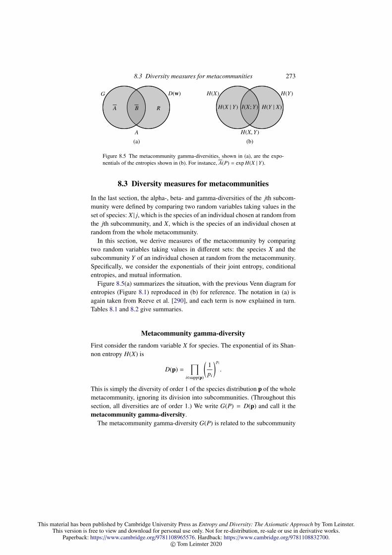
This material has been published by Cambridge University Press as Entropy and Diversity: The Axiomatic Approach by Tom Leinster.This version is free to view and download for personal use only. Not for re-distribution, re-sale or use in derivative works.
Paperback: https://www.cambridge.org/9781108965576. Hardback: https://www.cambridge.org/9781108832700.© Tom Leinster 2020
8.3 Diversity measures for metacommunities 273
G D(w)
A B R
A
(a)
H(X) H(Y)
H(X | Y) I(X; Y) H(Y | X)
H(X,Y)
(b)
Figure 8.5 The metacommunity gamma-diversities, shown in (a), are the expo-nentials of the entropies shown in (b). For instance, A(P) = exp H(X | Y).
8.3 Diversity measures for metacommunities
In the last section, the alpha-, beta- and gamma-diversities of the jth subcom-munity were defined by comparing two random variables taking values in theset of species: X | j, which is the species of an individual chosen at random fromthe jth subcommunity, and X, which is the species of an individual chosen atrandom from the whole metacommunity.
In this section, we derive measures of the metacommunity by comparingtwo random variables taking values in different sets: the species X and thesubcommunity Y of an individual chosen at random from the metacommunity.Specifically, we consider the exponentials of their joint entropy, conditionalentropies, and mutual information.
Figure 8.5(a) summarizes the situation, with the previous Venn diagram forentropies (Figure 8.1) reproduced in (b) for reference. The notation in (a) isagain taken from Reeve et al. [290], and each term is now explained in turn.Tables 8.1 and 8.2 give summaries.
Metacommunity gamma-diversity
First consider the random variable X for species. The exponential of its Shan-non entropy H(X) is
D(p) =∏
i∈supp(p)
(1pi
)pi
.
This is simply the diversity of order 1 of the species distribution p of the wholemetacommunity, ignoring its division into subcommunities. (Throughout thissection, all diversities are of order 1.) We write G(P) = D(p) and call it themetacommunity gamma-diversity.
The metacommunity gamma-diversity G(P) is related to the subcommunity
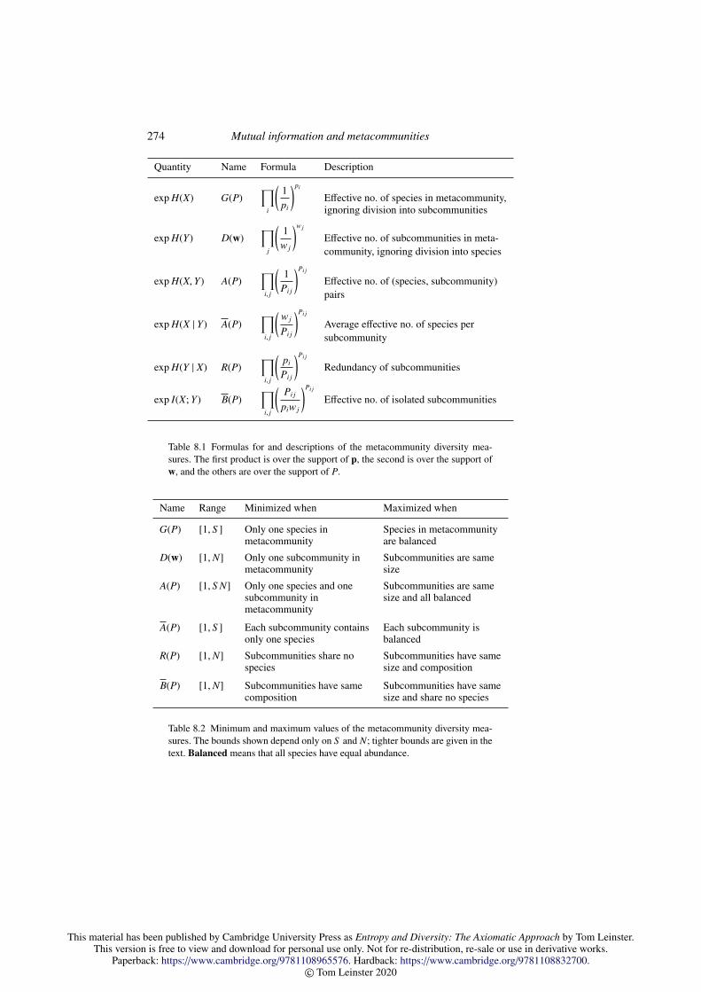
This material has been published by Cambridge University Press as Entropy and Diversity: The Axiomatic Approach by Tom Leinster.This version is free to view and download for personal use only. Not for re-distribution, re-sale or use in derivative works.
Paperback: https://www.cambridge.org/9781108965576. Hardback: https://www.cambridge.org/9781108832700.© Tom Leinster 2020
274 Mutual information and metacommunities
Quantity Name Formula Description
exp H(X) G(P)∏
i
(1pi
)pi
Effective no. of species in metacommunity,ignoring division into subcommunities
exp H(Y) D(w)∏
j
(1
w j
)w j
Effective no. of subcommunities in meta-community, ignoring division into species
exp H(X,Y) A(P)∏
i, j
(1
Pi j
)Pi j
Effective no. of (species, subcommunity)pairs
exp H(X | Y) A(P)∏
i, j
(w j
Pi j
)Pi j
Average effective no. of species persubcommunity
exp H(Y | X) R(P)∏
i, j
(pi
Pi j
)Pi j
Redundancy of subcommunities
exp I(X; Y) B(P)∏
i, j
(Pi j
piw j
)Pi j
Effective no. of isolated subcommunities
Table 8.1 Formulas for and descriptions of the metacommunity diversity mea-sures. The first product is over the support of p, the second is over the support ofw, and the others are over the support of P.
Name Range Minimized when Maximized when
G(P) [1, S ] Only one species in Species in metacommunitymetacommunity are balanced
D(w) [1,N] Only one subcommunity in Subcommunities are samemetacommunity size
A(P) [1, S N] Only one species and one Subcommunities are samesubcommunity in size and all balancedmetacommunity
A(P) [1, S ] Each subcommunity contains Each subcommunity isonly one species balanced
R(P) [1,N] Subcommunities share no Subcommunities have samespecies size and composition
B(P) [1,N] Subcommunities have same Subcommunities have samecomposition size and share no species
Table 8.2 Minimum and maximum values of the metacommunity diversity mea-sures. The bounds shown depend only on S and N; tighter bounds are given in thetext. Balanced means that all species have equal abundance.

This material has been published by Cambridge University Press as Entropy and Diversity: The Axiomatic Approach by Tom Leinster.This version is free to view and download for personal use only. Not for re-distribution, re-sale or use in derivative works.
Paperback: https://www.cambridge.org/9781108965576. Hardback: https://www.cambridge.org/9781108832700.© Tom Leinster 2020
8.3 Diversity measures for metacommunities 275
gamma-diversities γ1(P), . . . , γN(P) as follows:
G(P) =∏
i, j : i∈supp(p)
(1pi
)Pi j
=∏
j
γ j(P)w j
= M0
(w,
(γ1(P), . . . , γN(P)
)). (8.9)
Here we have used the definition of pi as∑
j Pi j and the formula (8.7) forγ j(P). So, the metacommunity gamma-diversity G(P) is the geometric meanof the subcommunity gamma-diversities γ j(P), weighted by the sizes of thesubcommunities.
In this sense, the subcommunity gamma-diversity γ j(P) is the mean contri-bution per individual of the jth subcommunity to the metacommunity diversity.
The metacommunity gamma-diversity is constrained by the bounds
1 ≤ G(P) ≤ S ,
by Lemma 2.4.3. It attains the lower bound G(P) = 1 when the metacommu-nity consists of a single species, and the upper bound G(P) = S when all Sspecies have equal abundance in the metacommunity (regardless of how theyare distributed across the subcommunities).
Now consider the random variable Y for subcommunities. The exponentialof H(Y) is
D(w) =∏
j∈supp(w)
(1
w j
)w j
.
It measures how evenly the population is distributed across the subcommuni-ties (regardless of how it is distributed across species). It is bounded by
1 ≤ D(w) ≤ N
(by Lemma 2.4.3 again), with D(w) = 1 when the metacommunity containsonly one nonempty subcommunity and D(w) = N when the populations of theN subcommunities are of equal size.
Metacommunity alpha-diversities
The joint entropy H(X,Y) has exponential
D(P) =∏
(i, j)∈supp(P)
(1
Pi j
)Pi j
.
This material has been published by Cambridge University Press as Entropy and Diversity: The Axiomatic Approach by Tom Leinster.This version is free to view and download for personal use only. Not for re-distribution, re-sale or use in derivative works.
Paperback: https://www.cambridge.org/9781108965576. Hardback: https://www.cambridge.org/9781108832700.© Tom Leinster 2020
276 Mutual information and metacommunities
Here we are treating the S × N matrix P as a probability distribution on theset 1, . . . , S × 1, . . . ,N. So, D(P) is the effective number of (species, sub-community) pairs, in the sense of Section 2.4. It is the species diversity thatthe metacommunity would have if individuals in different subcommunitieswere decreed to be of different species (as in the island scenario). We writeA(P) = D(P) and call it the raw metacommunity alpha-diversity.
Since A(P) measures diversity as if no species were shared between sub-communities, it overestimates the true diversity. Indeed, taking exponentials inthe inequalities
H(X) ≤ H(X,Y) ≤ H(X) + H(Y)
of Proposition 8.1.12(i) gives
G(P) ≤ A(P) ≤ D(w)G(P). (8.10)
The upper bound states that the factor of overestimation is at most D(w), theeffective number of subcommunities.
The minimum value A(P) = G(P) occurs when H(X,Y) = H(X), whichby Proposition 8.1.12(ii) means that Y is determined by X: the subcommunityis determined by the species. So, A(P) = G(P) when no species are sharedbetween subcommunities.
The maximum value A(P) = D(w)G(P) occurs when H(X,Y) = H(X) +
H(Y). By Proposition 8.1.12(i), this is true just when X and Y are independent.Equivalently, A(P) attains its maximum when the metacommunity is well-mixed, meaning that each of the subcommunity species distributions P• j/w j
is equal to the metacommunity species distribution p.In summary: A(P) does not overestimate G(P) at all when the subcommuni-
ties share no species, whereas the overestimation is most pronounced when allof the subcommunities have identical composition.
Since 1 ≤ G(P) ≤ S and 1 ≤ D(w) ≤ N, the inequalities (8.10) imply thecruder bounds
1 ≤ A(P) ≤ S N.
This conforms with the interpretation of A(P) as the effective number of(species, subcommunity) pairs. The minimum A(P) = 1 is attained when thereis only one species present and only one nonempty subcommunity. The maxi-mum A(P) = S N is attained when the metacommunity is well-mixed and thesubcommunities all have the same size.
Next consider conditional entropy. By Lemma 8.1.3(i), the conditional en-

This material has been published by Cambridge University Press as Entropy and Diversity: The Axiomatic Approach by Tom Leinster.This version is free to view and download for personal use only. Not for re-distribution, re-sale or use in derivative works.
Paperback: https://www.cambridge.org/9781108965576. Hardback: https://www.cambridge.org/9781108832700.© Tom Leinster 2020
8.3 Diversity measures for metacommunities 277
tropy H(X | Y) is given by
H(X | Y) =∑
i, j : Pr(i, j)>0
Pr(i, j) logPr( j)
Pr(i, j).
The normalized metacommunity alpha-diversity A(P) is its exponential:
A(P) = exp H(X | Y) =∏
i, j : Pi j>0
(w j
Pi j
)Pi j
. (8.11)
To understand A, we use one of the other formulas for conditional entropy:
H(X | Y) =∑
j : Pr( j)>0
Pr( j)H(X | j) (8.12)
(Lemma 8.1.3(ii)). The random variable X | j is the species of a random in-dividual from the jth subcommunity, so taking exponentials throughout equa-tion (8.12) gives
A(P) =∏
j : w j>0
α j(P)w j
= M0
(w,
(α1(P), . . . , αN(P)
)). (8.13)
Hence A(P) is the geometric mean of the individual subcommunity diversitiesα j(P), weighted by their sizes. It is therefore an alpha-diversity in the tradi-tional sense (Remark 3.3.9 and p. 269).
To find the maximum and minimum values of A, we take exponentialsthroughout the inequalities
0 ≤ H(X | Y) ≤ H(X)
(Proposition 8.1.12(ii)). This gives
1 ≤ A(P) ≤ G(P), (8.14)
with A(P) = 1 when each subcommunity contains at most one species andA(P) = G(P) when the metacommunity is well-mixed. Since G(P) ≤ S , wealso have the cruder bounds
1 ≤ A(P) ≤ S ,
with A(P) = S when each subcommunity contains all S species in equal pro-portions.
The raw and normalized metacommunity alpha-diversities, A(P) and A(P),are linked by the equation
A(P) = A(P)/D(w), (8.15)

This material has been published by Cambridge University Press as Entropy and Diversity: The Axiomatic Approach by Tom Leinster.This version is free to view and download for personal use only. Not for re-distribution, re-sale or use in derivative works.
Paperback: https://www.cambridge.org/9781108965576. Hardback: https://www.cambridge.org/9781108832700.© Tom Leinster 2020
278 Mutual information and metacommunities
Quantity Name (i) (ii) (iii) (iv)Well-mixed Only one Subcomms Isolatedmetacomm subcomm are species subcomms
exp H(X) G(P) D(p) D(p) D(p) D(p)
exp H(Y) D(w) D(w) 1 D(p) D(w)
exp H(X,Y) A(P) D(p)D(w) D(p) D(p) D(w)A(P)
exp H(X | Y) A(P) D(p) D(p) 1 A(P)
exp H(Y | X) R(P) D(w) 1 1 1
exp I(X; Y) B(P) 1 1 D(p) D(w)
Table 8.3 Summary of Examples 8.3.1 and 8.3.2.
which is the exponential of the definition
H(X | Y) = H(X,Y) − H(Y)
of conditional entropy.
Examples 8.3.1 Here we take the four running examples of Section 8.1 andtranslate them into ecological terms. The results below follow immediatelyfrom those examples, and are summarized in the first few rows of Table 8.3.
i. Suppose that the metacommunity is well-mixed. Then P = p⊗w and A(P) =
D(P) = D(p)D(w). Each subcommunity has the same species compositionas the metacommunity, so the mean subcommunity diversity A(P) is thesame as the metacommunity diversity G(P).
ii. Suppose that the metacommunity consists of a single subcommunity. ThenN = 1, w = (1), and P = p. The effective number A(P) of (species, subcom-munity) pairs is just the effective number D(p) of species, and since there isonly one subcommunity, the average subcommunity diversity A(P) is alsoD(p).
iii. Suppose that the subcommunities are exactly the species. Thus, N = S ,w = p, and P is the diagonal matrix with entries p1, . . . , pS . The effec-tive number A(P) of (species, subcommunity) pairs is again just D(p), butsince each subcommunity has a diversity of 1, the average subcommunitydiversity A(P) is now 1.
iv. Finally, suppose that all subcommunities are isolated (share no species).Nothing special can be said about A(P), the mean subcommunity diversity,since it is unaffected by the degree of overlap of species between subcom-munities. As always, A(P) = D(w)A(P).

This material has been published by Cambridge University Press as Entropy and Diversity: The Axiomatic Approach by Tom Leinster.This version is free to view and download for personal use only. Not for re-distribution, re-sale or use in derivative works.
Paperback: https://www.cambridge.org/9781108965576. Hardback: https://www.cambridge.org/9781108832700.© Tom Leinster 2020
8.3 Diversity measures for metacommunities 279
The redundancy of a metacommunity
We have already considered one conditional entropy, H(X | Y). The other,
H(Y | X) =∑
i, j : Pr(i, j)>0
Pr(i, j) logPr(i)
Pr(i, j),
has exponential
R(P) =∏
i, j : Pi j>0
(pi
Pi j
)Pi j
. (8.16)
This is the redundancy of the metacommunity. The word is meant in the fol-lowing sense: if some subcommunities were to be destroyed, how much of thediversity in the metacommunity would be preserved? High redundancy meansthat there is enough repetition of species across subcommunities that loss ofsome subcommunities would probably not cause great loss of diversity.
We now justify this interpretation. For each species i, consider the relativeabundances Pi1, . . . , PiN of that species within the N subcommunities, and nor-malize to obtain a probability distribution
Pi •/pi = (Pi1/pi, . . . , PiN/pi)
on the set 1, . . . ,N of subcommunities. (We assume in this explanation thatpi > 0.) Then D(Pi •/pi) measures the extent to which the ith species is spreadevenly across the subcommunities; for instance, it takes its maximum value Nwhen there is the same amount of species i in every subcommunity. This is the‘redundancy’ of the ith species.
To obtain a measure of the redundancy of the whole metacommunity, wetake the geometric mean ∏
i∈supp(p)
D(Pi •/pi)pi (8.17)
of the redundancies of the species, weighted by their relative abundances. Butthis is exactly R(P), since, using Lemma 8.1.3(ii),∏
i∈supp(p)
D(Pi •/pi)pi = exp( ∑
i∈supp(p)
piH(Pi •/pi))
= exp( ∑
i : Pr(i)>0
Pr(i)H(Y | i))
= exp H(Y | X)
= R(P).

This material has been published by Cambridge University Press as Entropy and Diversity: The Axiomatic Approach by Tom Leinster.This version is free to view and download for personal use only. Not for re-distribution, re-sale or use in derivative works.
Paperback: https://www.cambridge.org/9781108965576. Hardback: https://www.cambridge.org/9781108832700.© Tom Leinster 2020
280 Mutual information and metacommunities
In conclusion, R(P) is the average species redundancy (8.17): the effectivenumber of subcommunities across which a typical species is spread.
A different way to understand redundancy is through the equation
R = A/G, (8.18)
which is the exponential of the definition
H(Y | X) = H(X,Y) − H(X)
of conditional entropy. The gamma-diversity G(P) is the effective number ofspecies in the metacommunity, whereas A(P) is the effective number of speciesif we pretend that individuals in different subcommunities are always of differ-ent species. The amount by which A(P) overestimates G(P) reflects the extentto which species are, in reality, shared across subcommunities: thus, it mea-sures redundancy.
Bounds on the redundancy can be obtained by dividing inequalities (8.10)by G(P). This gives
1 ≤ R(P) ≤ D(w),
with the same extremal cases as for (8.10): redundancy takes its minimumvalue of 1 when no species are shared between subcommunities, and its maxi-mum value of D(w) when the species distributions in the subcommunities areall the same. It follows that
1 ≤ R(P) ≤ N,
with R(P) = N when the subcommunities have not only the same composition,but also the same size.
Metacommunity beta-diversity
Finally, consider the mutual information I(X; Y). By Lemma 8.1.7(i), its expo-nential B(P) is given by
B(P) =∏
i, j : Pi j>0
(Pi j
piw j
)Pi j
.
This is the metacommunity beta-diversity. (In Reeve et al. [290], it is calledthe ‘normalized’ beta-diversity, and there is also a ‘raw’ beta-diversity B(P),not treated here.) By the discussion of mutual information in Section 8.1, B(P)can be understood as the exponential of the amount of information that knowl-edge of an individual’s species gives us about its subcommunity – or equiva-lently, vice versa.

This material has been published by Cambridge University Press as Entropy and Diversity: The Axiomatic Approach by Tom Leinster.This version is free to view and download for personal use only. Not for re-distribution, re-sale or use in derivative works.
Paperback: https://www.cambridge.org/9781108965576. Hardback: https://www.cambridge.org/9781108832700.© Tom Leinster 2020
8.3 Diversity measures for metacommunities 281
Loosely, then, B(P) measures the alignment between subcommunity struc-ture and species structure. It is a beta-diversity in the traditional sense of Re-mark 3.3.9 and p. 269.
By Proposition 8.1.12(iii) on mutual information,
1 ≤ B(P) ≤ minG(P),D(w). (8.19)
The minimum B(P) = 1 is attained when X and Y are independent, thatis, the metacommunity is well-mixed. In that case, knowing an individual’sspecies does not help us to guess its subcommunity, nor vice versa. By Propo-sition 8.1.12(iii), there are two cases in which the maximum is attained. Oneis where X is determined by Y , that is, there is at most one species in eachsubcommunity. Then by Example 8.1.4(iv),
B(P) = G(P) ≤ D(w).
In this case, knowing the subcommunity to which an individual belongs en-ables us to infer its species with certainty. The other case in which the max-imum is attained is where Y is determined by X, that is, the subcommunitiesare isolated. Then
B(P) = D(w) ≤ G(P)
by Example 8.1.4(iv) again, and knowing an individual’s species enables us toinfer its subcommunity with certainty.
We can also interpret B as the effective number of isolated subcommunities.Indeed, since 1 ≤ D(w) ≤ N, the inequalities (8.19) imply that
1 ≤ B(P) ≤ N. (8.20)
The maximum B(P) = N occurs when the N subcommunities are isolatedand of equal size. We will see in Proposition 8.4.8 and Corollary 8.4.10 thatB satisfies a chain rule and a replication principle, supporting the effectivenumber interpretation.
For yet another viewpoint on B, recall from equations (8.5) that
H(X | Y) + I(X; Y) = H(X).
Taking exponentials throughout gives
A B = G, (8.21)
that is,
alpha-diversity × beta-diversity = gamma-diversity.
This equation partitions the diversity of the metacommunity (gamma) into two
This material has been published by Cambridge University Press as Entropy and Diversity: The Axiomatic Approach by Tom Leinster.This version is free to view and download for personal use only. Not for re-distribution, re-sale or use in derivative works.
Paperback: https://www.cambridge.org/9781108965576. Hardback: https://www.cambridge.org/9781108832700.© Tom Leinster 2020
282 Mutual information and metacommunities
components: the average diversity within subcommunities (alpha) and the vari-ation between subcommunities (beta). The general principle has a long history,going back to the foundational work of Whittaker (p. 321 of [348] and p. 232of [349]).
From equations (8.21), (8.15) and (8.18), it follows that
B(P) =G(P)
A(P)=
G(P)D(w)A(P)
=D(w)R(P)
,
giving
B(P) =D(w)R(P)
.
So when the subcommunity sizes w are fixed, the effective number B(P) ofisolated subcommunities is inversely proportional to the redundancy R(P).This is reasonable: R(P) measures overlap of species between subcommuni-ties, whereas B(P) measures how disjoint the subcommunities are.
(Matters are more subtle outside the case q = 1, Z = I to which we haveconfined ourselves. When q , 1 in the work of Reeve et al., the dependencybetween B and R breaks down, in the strong sense that the two quantities nolonger determine one another; they convey different information.)
Examples 8.3.2 We return to the four scenarios of Examples 8.3.1, findingthe redundancy R(P) and metacommunity beta-diversity B(P). The results aresummarized in Table 8.3.
i. A well-mixed metacommunity is maximally redundant (R(P) = D(w)),since all subcommunities are identical. For the same reason, the effectivenumber B(P) of isolated subcommunities is just 1.
ii. If the metacommunity consists of a single subcommunity (N = 1) then theredundancy R(P) and effective number B(P) of isolated subcommunitiesboth take their minimum values of 1.
iii. Suppose that the subcommunities are exactly the species. Then the meta-community is minimally redundant (R(P) = 1), reflecting the fact that eachspecies is present in just one subcommunity: losing any of the subcommu-nities means losing a species. And since subcommunities are species, theeffective number B(P) of isolated subcommunities is the effective numberD(p) of species.
iv. More generally, suppose that all subcommunities are isolated. The redun-dancy is minimal (R(P) = 1), since no species is repeated across subcom-munities. The effective number B(P) of isolated subcommunities is simplythe diversity D(w) of the subcommunity distribution w, which is reasonablesince, in fact, the subcommunities are isolated.

This material has been published by Cambridge University Press as Entropy and Diversity: The Axiomatic Approach by Tom Leinster.This version is free to view and download for personal use only. Not for re-distribution, re-sale or use in derivative works.
Paperback: https://www.cambridge.org/9781108965576. Hardback: https://www.cambridge.org/9781108832700.© Tom Leinster 2020
8.4 Properties of the metacommunity measures 283
Just as the metacommunity gamma-diversity G(P) is the geometric meanof the subcommunity gamma-diversities γ j(P), and just as the metacom-munity alpha-diversity A(P) is the geometric mean of the subcommunityalpha-diversities α j(P), the metacommunity beta-diversity B(P) is the geo-metric mean of the subcommunity beta-diversities β j(P). Indeed, recall fromLemma 8.1.7(ii) that
I(X; Y) =∑
j : Pr( j)>0
Pr( j)H((X | j) ‖ X
).
Taking exponentials throughout gives
B(P) =∏
j : w j>0
β j(P)w j
= M0
(w,
(β1(P), . . . , βN(P)
)), (8.22)
as claimed.We have seen that β j(P) measures how unusual the jth subcommunity is in
the context of the metacommunity. Taking the geometric mean over all sub-communities gives B(P), which is therefore an overall measure of the atypical-ity or isolation of the subcommunities within the metacommunity.
Further connections between beta-diversity and information-theoretic quan-tities are described in the first appendix of the paper [290] of Reeve et al.
8.4 Properties of the metacommunity measures
In this chapter so far, we have introduced a system of measures of the diversityand structure of a metacommunity, and explained their behaviour in a varietyof hypothetical examples. But just as a measure of the diversity of a singlecommunity should not be accepted or used until it can be shown to behavelogically (Section 2.4), the metacommunity measures should also be requiredto have sensible logical and algebraic properties. Here we show that they do.
Independence
We begin by showing that the alpha-diversity A and beta-diversity B are in-dependent – not in the sense of probability theory, but in the sense of certainknowledge. An informal example illustrates the idea. Assume for simplicitythat every person in the world is either dark-haired or fair-haired, and eitherbrown-eyed or blue-eyed. These two variables, hair colour and eye colour,are not independent in the probabilistic sense: people with dark hair are more

This material has been published by Cambridge University Press as Entropy and Diversity: The Axiomatic Approach by Tom Leinster.This version is free to view and download for personal use only. Not for re-distribution, re-sale or use in derivative works.
Paperback: https://www.cambridge.org/9781108965576. Hardback: https://www.cambridge.org/9781108832700.© Tom Leinster 2020
284 Mutual information and metacommunities
likely to have dark eyes. However, they are independent in a weaker sense:knowing an individual’s hair colour gives no certain knowledge of their eyecolour, nor vice versa. All four combinations occur.
The formal definition is as follows.
Definition 8.4.1 Let J, K and L be sets. Functions
K
J
κ 77
λ '' L
are independent if for all k ∈ κJ and ` ∈ λJ, there exists j ∈ J such thatκ( j) = k and λ( j) = `.
For κ and λ to be independent means that if I choose in secret an element j ofJ, and tell you the value of κ( j) ∈ K, you gain no certain information about thevalue of λ( j). (For by definition of independence, the image under λ of the fibreκ−1κ( j) is no smaller than the whole image λJ.) Of course, the same is alsotrue with the roles of κ and λ reversed. In the informal example above, J is theset of all people, K = dark hair, fair hair, and L = brown eyes, blue eyes.
We have discussed the general goal of decomposing any measure ofmetacommunity diversity (any ‘gamma-diversity’) into within-group (alpha)and between-group (beta) components. The alpha-diversity and beta-diversityshould be independent, otherwise the word ‘decomposition’ is not deserved:certain values of alpha would exclude certain values of beta, and vice versa.This requirement has been recognized in ecology since at least the 1984 workof Wilson and Shmida [357]. As Jost put it:
Since [alpha- and beta-diversity] measure completely different aspects ofregional diversity, they must be free to vary independently; alpha shouldnot put mathematical constraints on the possible values of beta, and viceversa. If beta depended on alpha, it would be impossible to compare betadiversities of regions whose alpha diversities differed.
([165], p. 2428.)We will show that the decomposition
A B = G
(equation (8.21)) passes this test. Since the number N of subcommunities isusually known in advance, but the number S of species may not be, we interpret

This material has been published by Cambridge University Press as Entropy and Diversity: The Axiomatic Approach by Tom Leinster.This version is free to view and download for personal use only. Not for re-distribution, re-sale or use in derivative works.
Paperback: https://www.cambridge.org/9781108965576. Hardback: https://www.cambridge.org/9781108832700.© Tom Leinster 2020
8.4 Properties of the metacommunity measures 285
independence as meaning that for each N ≥ 1, the functions
R∐S≥1
∆S N
A 77
B ''R
are independent. Here ∆S N is understood as the set of S × N matrices P ofnonnegative reals summing to 1, so that the disjoint union
∐S≥1 ∆S N is the set
of all such matrices P with N columns and any number of rows.Independence of these two functions means that given a metacommunity
divided into a known number N of subcommunities, knowledge of the meandiversity A(P) of the subcommunities does not restrict the range of possiblevalues of B(P), the effective number of isolated subcommunities. Thus, B(P)can still take all the values that it could have taken had we not known A(P).Equivalently, independence means that knowing the value of B(P) does notenable us to deduce anything about A(P). We prove this now.
Proposition 8.4.2 (Independence of alpha- and beta-diversities) For eachN ≥ 1, the functions
∐S≥1
∆S N
A //
B// R
are independent.
Proof We have already shown that A(P) ≥ 1 and 1 ≤ B(P) ≤ N for all P ∈∐S≥1 ∆S N (inequalities (8.14) and (8.20)). So it suffices to show that given any
a ∈ [1,∞) and b ∈ [1,N], there exist some S ≥ 1 and some S × N matrixP ∈ ∆S N such that A(P) = a and B(P) = b.
One way to do this is as follows. Choose an integer T ≥ a. The diversitymeasure D : ∆T → R is continuous (Lemma 2.4.4) with minimum 1 and max-imum T (Lemma 2.4.3), so we can choose some t ∈ ∆T such that D(t) = a.Similarly, we can choose some w ∈ ∆N such that D(w) = b.
Now consider a metacommunity made up of N subcommunities of relativesizes w1, . . . ,wN , with no shared species, where each subcommunity contains

This material has been published by Cambridge University Press as Entropy and Diversity: The Axiomatic Approach by Tom Leinster.This version is free to view and download for personal use only. Not for re-distribution, re-sale or use in derivative works.
Paperback: https://www.cambridge.org/9781108965576. Hardback: https://www.cambridge.org/9781108832700.© Tom Leinster 2020
286 Mutual information and metacommunities
T species in proportions t1, . . . , tT . Thus, there are T N species in all, and
P =
w1t1 0 0...
... · · ·...
w1tT 0 00 w2t1 0...
... · · ·...
0 w2tT 0
......
...
0 0 wN t1...
... · · ·...
0 0 wN tT
.
The species distribution P• j/w j in the jth subcommunity is
(0, . . . , 0, t1, . . . , tT , 0, . . . , 0),
so its diversity α j(P) is D(t) = a. But A(P) is an average of α1(P), . . . , αN(P)(equation (8.13)), so A(P) = a. Moreover, the subcommunities are isolated, soby Example 8.3.2(iv), B(P) = D(w) = b.
In the same sense, the average subcommunity diversity A and the redun-dancy R are independent:
Proposition 8.4.3 (Independence of alpha-diversity and redundancy) Foreach N ≥ 1, the functions
∐S≥1
∆S N
A //
R// R
are independent.
Proof The proof is similar to that of the last proposition. We have already seenthat A(P) ∈ [1,∞) and R(P) ∈ [1,N] for all P ∈
∐S≥1 ∆S N . So it suffices to
show that given a ∈ [1,∞) and r ∈ [1,N], there exist an integer S ≥ 1 and anS × N matrix P ∈ ∆S N such that A(P) = a and R(P) = r.
To prove this, choose an integer S ≥ a and distributions p ∈ ∆S ,w ∈ ∆N
such that D(p) = a and D(w) = r. Consider a well-mixed metacommunitymade up of N subcommunities of relative sizes w1, . . . ,wN , each with the sameS species in proportions p1, . . . , pS . Thus, P = p ⊗ w. By Examples 8.3.1(i)and 8.3.2(i), A(P) = D(p) = a and R(P) = D(w) = r.

This material has been published by Cambridge University Press as Entropy and Diversity: The Axiomatic Approach by Tom Leinster.This version is free to view and download for personal use only. Not for re-distribution, re-sale or use in derivative works.
Paperback: https://www.cambridge.org/9781108965576. Hardback: https://www.cambridge.org/9781108832700.© Tom Leinster 2020
8.4 Properties of the metacommunity measures 287
Identical subcommunities
When we were analysing the diversity of a single community, we argued thatany similarity-sensitive diversity measure should be unchanged if a species isreclassified into two identical smaller species, and we proved that the diversitymeasures DZ
q do indeed enjoy this property (Lemma 6.2.9, Example 6.2.10,and the text afterwards). It follows by continuity that if a species is divided intotwo nearly identical parts, the diversity increases only slightly. This is sensiblebehaviour, given that diversity is intended to measure the effective number ofcompletely dissimilar species (p. 183).
The same principle applies to B, the effective number of isolated subcom-munities in a metacommunity. Dividing a subcommunity into two smaller sub-communities of identical composition should not change B. In other words,the effective number of isolated subcommunities should not be changed by thepresence or absence of boundaries between subcommunities that are identical.The average subcommunity diversity A should be similarly unaffected.
In summary, then, the decomposition of global diversity into within-subcommunity and between-subcommunity components,
A B = G, (8.23)
should be unaffected by arbitrary decisions about where subcommunity bound-aries lie. This is best explained by example.
Example 8.4.4 Suppose that we are interested in the tree diversity of a coun-try that is divided into administrative districts with no ecological significance.Suppose further that in a particular pair of neighbouring districts, the distribu-tions of tree species are identical. In that case, the partitioning (8.23) of theoverall diversity into within- and between-district components should be thesame as if the neighbouring districts had been merged into one. The effectivenumber of isolated subcommunities should be invariant under the removal oraddition of ecologically irrelevant boundaries.
Example 8.4.5 Suppose that we are studying the various species of grass on ahillside. To investigate the varying abundances of different species at differentaltitudes, we divide the hillside into height bands (0–10m, 10–20m, etc.) andregard them as subcommunities.
The beta-diversity B measures the effective number of isolated or disjointsubcommunities, so if it turns out that the bottom two height bands have thesame species distribution, then B should be the same as if they were consideredas a single band (0–20m).
In short, we require that the decomposition (8.23) of metacommunity diver-

This material has been published by Cambridge University Press as Entropy and Diversity: The Axiomatic Approach by Tom Leinster.This version is free to view and download for personal use only. Not for re-distribution, re-sale or use in derivative works.
Paperback: https://www.cambridge.org/9781108965576. Hardback: https://www.cambridge.org/9781108832700.© Tom Leinster 2020
288 Mutual information and metacommunities
sity into alpha and beta components is ecologically meaningful, not an artefactof the particular subcommunity division chosen. As far as possible, the de-composition should be independent of resolution (that is, how fine or coarsethe subcommunity division may be). In general, the finer the division one uses,the more variation between subcommunities one will observe. But if a subcom-munity is ecologically uniform (has the same species distribution throughout)then dividing it further should make no difference to B or A.
We now give a formal statement and proof of the desired invariance prop-erty of A, B and G. To minimize notational overhead, we consider splitting asingle subcommunity into two rather than splitting every subcommunity intoan arbitrary number of smaller parts; but the general case follows by induction.
In the standard notation of this chapter, take an S × N matrix P ∈ ∆S N withspecies distribution p ∈ ∆S and subcommunity size distribution w ∈ ∆N , sothat pi =
∑j Pi j and w j =
∑i Pi j. Split the last subcommunity into two parts
of relative sizes t and 1 − t (where 0 ≤ t ≤ 1), and suppose that the two partshave the same species distribution. Then the new relative abundance matrix isthe S × (N + 1) matrix P′ given by
P′i j =
Pi j if 1 ≤ j ≤ N − 1,
tPiN if j = N,
(1 − t)PiN if j = N + 1.
Proposition 8.4.6 (Identical subcommunities) In the situation described,
A(P′) = A(P), B(P′) = B(P), G(P′) = G(P).
(In Reeve et al. [290], the splitting of a subcommunity into smaller partswith the same species distribution is called ‘shattering’, so the result is that A,B and G are invariant under shattering.)
The idea behind the proof is that A is the average diversity of the subcom-munity of an individual chosen at random, and this quantity is unchanged if awell-mixed subcommunity is split into smaller parts.
Proof Write p′ ∈ ∆S and w′ ∈ ∆N+1 for the row- and column-sums of P′.Then for each i ∈ 1, . . . , S ,
p′i =
N−1∑j=1
Pi j + tPiN + (1 − t)PiN =
N∑j=1
Pi j = pi,

This material has been published by Cambridge University Press as Entropy and Diversity: The Axiomatic Approach by Tom Leinster.This version is free to view and download for personal use only. Not for re-distribution, re-sale or use in derivative works.
Paperback: https://www.cambridge.org/9781108965576. Hardback: https://www.cambridge.org/9781108832700.© Tom Leinster 2020
8.4 Properties of the metacommunity measures 289
so p′ = p, and for each j ∈ 1, . . . ,N + 1,
w′j =
S∑i=1
P′i j =
w j if j ≤ N − 1,
twN if j = N,
(1 − t)wN if j = N + 1.
First, G(P′) = D(p′) = D(p) = G(P), so G(P′) = G(P). (This is also clearinformally, since the definition of metacommunity gamma-diversity G does notrefer to the division into subcommunities.)
Next, to calculate A(P′), consider the subcommunity alpha-diversitiesα j(P′). For each j ∈ 1, . . . ,N + 1 such that w′j > 0, the species distribution ofsubcommunity j is
P′• j/w
′j =
P• j/w j if 1 ≤ j ≤ N − 1,
P•N/wN if j ∈ N,N + 1,
giving
α j(P′) =
α j(P) if 1 ≤ j ≤ N − 1,
αN(P) if j ∈ N,N + 1.
Equation (8.13) then gives
A(P′) = M0
(w′,
(α1(P′), . . . , αN(P′), αN+1(P′)
))= M0
((w1, . . . ,wN−1, twN , (1 − t)wN
),(α1(P), . . . , αN(P), αN(P)
))= M0
((w1, . . . ,wN−1,wN),
(α1(P), . . . , αN−1(P), αN(P)
))(8.24)
= A(P),
where in equation (8.24) we used the repetition property of the power means(Lemma 4.2.11). Hence A(P′) = A(P).
Finally, by equation (8.23),
B(P′) =G(P′)
A(P′)=
G(P)
A(P)= B(P),
completing the proof.
Although A, B and G have the invariance property just established, the re-dundancy R and raw metacommunity alpha-diversity A do not:
Example 8.4.7 Consider a metacommunity consisting of a single subcommu-nity, as in Examples 8.3.1(ii) and 8.3.2(ii). Suppose that it is ecologically ho-mogeneous, and split it arbitrarily into new subcommunities of relative sizes

This material has been published by Cambridge University Press as Entropy and Diversity: The Axiomatic Approach by Tom Leinster.This version is free to view and download for personal use only. Not for re-distribution, re-sale or use in derivative works.
Paperback: https://www.cambridge.org/9781108965576. Hardback: https://www.cambridge.org/9781108832700.© Tom Leinster 2020
290 Mutual information and metacommunities
w1, . . . ,wN . Then the species distributions in the new subcommunities are iden-tical. As we see from columns (i) and (ii) of Table 8.3, the global diversity G,average subcommunity diversity A and effective number B of isolated subcom-munities are the same before and after the division.
On the other hand, the effective number A of (species, subcommunity) pairsis greater by a factor of D(w) in the newly divided metacommunity. This is be-cause A counts individuals of the same species but different subcommunities asbeing in different groups, and therefore depends directly on the subcommunitydivisions, however arbitrary they may be. The redundancy R is also greaterby a factor of D(w) in the divided metacommunity, because it too measuresproperties of the subcommunity division (namely, the effective number of sub-communities that a typical species is spread across). So it is reasonable thatA and R increase when a subcommunity is split into smaller units, even whenthat subcommunity is well-mixed.
Chain rule, modularity and replication principle
For measures of the diversity of a single community, we have seen that themost important algebraic properties are the chain rule and the principles ofmodularity and replication. Here we show that versions of these propertiesalso hold for the metacommunity measures.
Consider a group of islands, each divided into several regions (Figure 8.6).Each island can be considered as a metacommunity, and has associated with itall the metacommunity measures A, A, R, B, etc., discussed above. On the otherhand, the whole island group can be considered as a metacommunity made upof regions, ignoring the intermediate level of islands. Can the redundancy ofthe whole island group be computed from the redundancies and relative sizesof the individual islands? If so, how? And the same questions can be asked forall the other metacommunity measures.
To give a precise statement of the problem and its solution, we need somenotation and terminology.
We consider a multicommunity divided into m metacommunities, whichhave no species in common. The kth metacommunity (1 ≤ k ≤ m) is furtherdivided into Nk subcommunities and S k species; the subcommunities of eachmetacommunity may have species in common. There are N1 + · · · + Nm sub-communities and S 1 + · · ·+ S m species in the multicommunity as a whole. Therelative sizes (that is, relative population abundances) of the metacommunitiesare denoted by x1, . . . , xm, so that x = (x1, . . . , xm) ∈ ∆m.
Write Pk for the relative abundance matrix of the kth metacommunity di-vided into its subcommunities. Thus, Pk is an S k × Nk matrix. Write pk ∈ ∆S k

This material has been published by Cambridge University Press as Entropy and Diversity: The Axiomatic Approach by Tom Leinster.This version is free to view and download for personal use only. Not for re-distribution, re-sale or use in derivative works.
Paperback: https://www.cambridge.org/9781108965576. Hardback: https://www.cambridge.org/9781108832700.© Tom Leinster 2020
8.4 Properties of the metacommunity measures 291
metacommunity 1
x1
metacommunity 2
x2
· · ·
· · ·
metacommunity m
xm
︸ ︷︷ ︸multicommunity
Figure 8.6 Terminology for the chain rule, modularity principle and replicationprinciple. A multicommunity is divided into m metacommunities, with no speciesin common, of relative sizes x1, . . . , xm. Each metacommunity is further dividedinto subcommunities, which may have species in common. In the example shown,there are m = 4 metacommunities, divided into N1 = 4, N2 = 5, N3 = 2 and N4 =
3 subcommunities, respectively. We may choose to ignore the metacommunitylevel and view the multicommunity as divided into
∑k Nk = 14 subcommunities.
for the relative abundance distribution of species in the kth metacommunity,and wk ∈ ∆Nk for the relative sizes of its subcommunities. Since the meta-communities share no species, the relative abundance matrix P? of the mul-ticommunity (with respect to its division into subcommunities, ignoring themetacommunity level) is the matrix block sum
P? = x1P1 ⊕ · · · ⊕ xmPm (8.25)
=
x1P1 0 · · · 0
0 x2P2 . . ....
.... . .
. . . 00 · · · 0 xmPm
.
The relative abundance distribution p? of species in the multicommunity isgiven by
p? = x1p1 ⊕ · · · ⊕ xmpm = x (p1, . . . ,pm) ∈ ∆S 1+···+S m ,
and the relative size distribution w? of the N1 + · · ·+ Nk subcommunities in the
This material has been published by Cambridge University Press as Entropy and Diversity: The Axiomatic Approach by Tom Leinster.This version is free to view and download for personal use only. Not for re-distribution, re-sale or use in derivative works.
Paperback: https://www.cambridge.org/9781108965576. Hardback: https://www.cambridge.org/9781108832700.© Tom Leinster 2020
292 Mutual information and metacommunities
multicommunity is given by
w? = x1w1 ⊕ · · · ⊕ xmwm = x (w1, . . . ,wm).
The main result is:
Proposition 8.4.8 (Chain rule) With notation as above,
G(P?) = D(x) ·∏
k
G(Pk)xk ,
D(w?) = D(x) ·∏
k
D(wk)xk ,
A(P?) = D(x) ·∏
k
A(Pk)xk ,
A(P?) =∏
k
A(Pk)xk ,
R(P?) =∏
k
R(Pk)xk ,
B(P?) = D(x) ·∏
k
B(Pk)xk ,
where the products are over all k ∈ 1, . . . ,m such that xk > 0.
Proof The statement on gamma-diversity is simply the chain rule for the di-versity of a single community (Corollary 2.4.8):
G(P?) = D(p?)
= D(x (p1, . . . ,pm)
)= D(x) ·
∏k
D(pk)xk
= D(x) ·∏
k
G(Pk)xk .
The same argument gives the formula for D(w?). It also gives the formula forA(P?), as follows. When the matrices P? and P1, . . . , Pm are regarded as finiteprobability distributions, equation (8.25) implies that P? can be obtained fromx (P1, . . . , Pm) by permutation of its entries and insertion of zeros. By thesymmetry and absence-invariance of D, it follows that
D(P?) = D(x (P1, . . . , Pm)
).
The chain rule for D then gives
D(P?) = D(x) ·∏
k
D(Pk)xk ,

This material has been published by Cambridge University Press as Entropy and Diversity: The Axiomatic Approach by Tom Leinster.This version is free to view and download for personal use only. Not for re-distribution, re-sale or use in derivative works.
Paperback: https://www.cambridge.org/9781108965576. Hardback: https://www.cambridge.org/9781108832700.© Tom Leinster 2020
8.4 Properties of the metacommunity measures 293
or equivalently,
A(P?) = D(x) ·∏
k
A(Pk)xk .
This proves the first three equations. Since the last three left-hand sides canbe calculated from the first three (Figure 8.5), the rest of the proof is routine.Indeed, by equation (8.15),
A(P?) =A(P?)D(w?)
=∏
k
(A(Pk)D(wk)
)xk
=∏
k
A(Pk)xk ,
and similarly, by equation (8.18),
R(P?) =A(P?)G(P?)
=∏
k
(A(Pk)G(Pk)
)xk
=∏
k
R(Pk)xk .
Finally, by equation (8.21),
B(P?) =G(P?)
A(P?)= D(x) ·
∏k
(G(Pk)
A(Pk)
)xk
= D(x) ·∏
k
B(Pk)xk ,
completing the proof.
In particular, each multicommunity measure (such as A(P?)) is determinedby the corresponding metacommunity measures (such as A(P1), . . . , A(Pm))and the relative sizes of the metacommunities (x1, . . . , xm). This is the modu-larity property of the measures G, A, A, R and B.
The formulas in Proposition 8.4.8 can be restated more compactly in termsof the value measure σ1 (defined in Section 7.1) and the geometric mean M0.Write
A(P•) =(A(P1), . . . , A(Pm)
)∈ Rm,
and similarly for the other measures. Then Proposition 8.4.8 states:
Corollary 8.4.9 In the notation of Proposition 8.4.8,
G(P?) = σ1(x,G(P•)
), D(w?) = σ1
(x,D(w•)
), A(P?) = σ1
(x, A(P•)
),
A(P?) = M0(x, A(P•)
), R(P?) = M0
(x,R(P•)
),
B(P?) = σ1(x, B(P•)
).
Here, the first row consists of exponentials of ordinary and joint entropies,the second of exponentials of conditional entropies, and the last of the expo-nential of mutual information.
An essential distinction is clear. The formulas in the first and third rows arevalue measures, meaning that the multicommunity measure G(P?) aggregates

This material has been published by Cambridge University Press as Entropy and Diversity: The Axiomatic Approach by Tom Leinster.This version is free to view and download for personal use only. Not for re-distribution, re-sale or use in derivative works.
Paperback: https://www.cambridge.org/9781108965576. Hardback: https://www.cambridge.org/9781108832700.© Tom Leinster 2020
294 Mutual information and metacommunities
the measures G(P1), . . . ,G(Pm) of the islands of which the multicommunityis comprised, and similarly for D(w?), A(P?) and B(P?). Those in the sec-ond row are means: A(P?) averages the island measures A(P1), . . . , A(Pm), andsimilarly for R(P?).
The point is clarified by considering a specific case. Suppose that the m is-lands are identical in almost every way: they have the same size, the same num-ber S of species, the same division into subcommunities, and the same speciesdistribution within each subcommunity. The only difference is that each islanduses a disjoint set of species. Thus, G(Pk), D(wk), A(Pk), A(Pk), R(Pk) andB(Pk) are all independent of k ∈ 1, . . . ,m, and x = um.
Corollary 8.4.10 (Replication) In this situation,
G(P?) = mG(P1), D(w?) = mD(w1), A(P?) = mA(P1),
A(P?) = A(P1), R(P?) = R(P1),
B(P?) = mB(P1).
Example 8.4.11 Take a single island divided into subcommunities, then makea copy of it, using a disjoint set of species for the copy. In the new, largersystem consisting of both islands, four of the metacommunity measures aretwice what they were for a single island: the effective number G of species, thediversity of the relative size distribution of the subcommunities, the effectivenumber A of (species, subcommunity) pairs, and the effective number B ofisolated subcommunities.
But the other two remain the same. The mean diversity of the subcommuni-ties, A, is unchanged, because the subcommunities on the second island havethe same abundance distributions as those on the first. The redundancy, R, isalso unchanged, because the two islands have no species in common. Put an-other way, the average spread of species across subcommunities is the same inthe two-island system as on either island individually.
8.5 All entropy is relative
The title of this section has two meanings. First, the definition of the entropyof a probability distribution on a finite set is implicitly relative to the uniformdistribution. Hence on a general measurable space, ordinary entropy does noteven make sense; only relative entropy does. This point was discussed in Sec-tion 3.4.
Here we explore a different meaning: that all of the entropies associated

This material has been published by Cambridge University Press as Entropy and Diversity: The Axiomatic Approach by Tom Leinster.This version is free to view and download for personal use only. Not for re-distribution, re-sale or use in derivative works.
Paperback: https://www.cambridge.org/9781108965576. Hardback: https://www.cambridge.org/9781108832700.© Tom Leinster 2020
8.5 All entropy is relative 295
with a pair of random variables – cross, joint, conditional, and mutual infor-mation – can be reduced to relative entropy. This reduction sheds new light onthe subcommunity and metacommunity diversity measures.
We examine each type of entropy in turn, beginning with ordinary Shannonentropy. Let X be a random variable taking values in a finite set X, and let UXdenote a random variable uniformly distributed in X. We have already seenthat
H(X) = log|X| − H(X ‖ UX) (8.26)
(Example 3.1.2), which expresses ordinary entropy in terms of relative entropytogether with the cardinality |X| of the set X.
For cross entropy, let X1 and X2 be random variables taking values in thesame finite set X. By equations (3.6) and (8.26),
H×(X1 ‖ X2) = H(X1 ‖ X2) + H(X1)
= log|X| + H(X1 ‖ X2) − H(X1 ‖ UX), (8.27)
expressing cross entropy in terms of relative entropy and |X|.Now let X and Y be random variables, not necessarily independent, taking
values in finite sets X and Y respectively. Thus, the random variable (X,Y)takes values in X ×Y. By equation (8.26), the joint entropy of X and Y is
H(X,Y) = log|X| + log|Y| − H((X,Y) ‖ UX ⊗ UY
), (8.28)
where ⊗ denotes the independent coupling of random variables (as in Re-mark 8.1.13). Here we have used the observation that UX ⊗ UY is uniformlydistributed on X ×Y.
By the explicit formula for mutual information in Lemma 8.1.7(i),
I(X; Y) = H((X,Y) ‖ X ⊗ Y
). (8.29)
Thus, mutual information is not merely expressible in terms of relative en-tropy; it is an instance of relative entropy. By Lemma 3.1.4 on relative entropy,I(X; Y) ≥ 0 with equality if and only if (X,Y) and X ⊗ Y are identically dis-tributed, that is, X and Y are independent. This gives another proof of the lowerbound in Proposition 8.1.12(iii).
It remains to consider conditional entropy.
Lemma 8.5.1 Take random variables V and W on the same sample space,with values in finite sets V and W respectively. Also take random variablesV ′ and W ′, with values inV andW respectively. Then
H((V,W) ‖ V ′ ⊗W ′
)= H
((V,W) ‖ V ⊗W ′) + H(V ‖ V ′).

This material has been published by Cambridge University Press as Entropy and Diversity: The Axiomatic Approach by Tom Leinster.This version is free to view and download for personal use only. Not for re-distribution, re-sale or use in derivative works.
Paperback: https://www.cambridge.org/9781108965576. Hardback: https://www.cambridge.org/9781108832700.© Tom Leinster 2020
296 Mutual information and metacommunities
Equations of this type are called Pythagorean identities (as in Theorem 4.2 ofCsiszar and Shields [74]), because of the features that relative entropy shareswith a squared distance (Section 3.4).
Proof By definition, the right-hand side is∑v,w : Pr(V=v,W=w)>0
Pr(V = v,W = w) logPr(V = v,W = w)
Pr(V = v) Pr(W ′ = w)
+∑
v : Pr(V=v)>0
Pr(V = v) logPr(V = v)Pr(V ′ = v)
.
But since Pr(V = v) =∑
w Pr(V = v,W = w), the second term is equal to∑v,w : Pr(V=v,W=w)>0
Pr(V = v,W = w) logPr(V = v)Pr(V ′ = v)
.
Collecting terms and cancelling gives the result.
We return to our setting of random variables X and Y taking values in finitesets X and Y. By equations (8.26) and (8.29), we can express the conditionalentropy as
H(X | Y) = H(X) − I(X; Y)
= log|X| −H(X ‖ UX) + H
((X,Y) ‖ X ⊗ Y
),
which by Lemma 8.5.1 gives a formula for conditional entropy in terms ofrelative entropy:
H(X | Y) = log|X| − H((X,Y) ‖ UX ⊗ Y
). (8.30)
For example, if we fix X, Y and Y but allow X to vary, the conditional entropyH(X | Y) is greatest when the relative entropy H
((X,Y) ‖UX ⊗ Y
)is least. This
happens when (X,Y) has the same distribution as UX ⊗ Y , that is, when X isindependent of Y and uniformly distributed.
We have now reduced each of the various kinds of entropy to relative en-tropy. The purpose of this reduction is to illuminate the various measures ofsubcommunity and metacommunity diversity. In this setting, relative entropyis replaced by relative diversity (introduced in Section 3.3), and the concept ofvalue (Chapter 7) also plays an important part. The results are summarized inTable 8.4.
As before in this chapter, let P ∈ ∆S N be an S × N matrix representingthe relative abundances of S species in N subcommunities, write p ∈ ∆S forthe overall relative abundance vector of the species, and write w ∈ ∆N for therelative sizes of the subcommunities. We will often want to refer to the relative

This material has been published by Cambridge University Press as Entropy and Diversity: The Axiomatic Approach by Tom Leinster.This version is free to view and download for personal use only. Not for re-distribution, re-sale or use in derivative works.
Paperback: https://www.cambridge.org/9781108965576. Hardback: https://www.cambridge.org/9781108832700.© Tom Leinster 2020
8.5 All entropy is relative 297
α j(P) = σ(P• j, 1S
)β j(P) = D
(P• j ‖ p
)γ j(P) = σ
(P• j, P• j/p
)A(P) = σ(P, 1S ⊗ w) B(P) = D(P ‖ p ⊗ w) G(P) = σ(p, 1S )
A(P) = σ(P, 1S ⊗ 1N) R(P) = σ(P,p ⊗ 1N)
Table 8.4 The subcommunity and metacommunity measures expressed in termsof relative diversity D(− ‖ −) and value σ.
abundance distribution P• j/w j of species in the jth subcommunity, so let uswrite
P• j = P• j/w j = (P1 j/w j, . . . , PS j/w j) ∈ ∆S
for each j ∈ 1, . . . ,N such that w j > 0.We begin with beta-diversity. The subcommunity measure β j(P) is the rela-
tive diversity
β j(P) = D(P• j ‖ p
)by definition (equation (8.6)); its interpretation was discussed in Sections 3.3and 8.2. The metacommunity measure B(P), which is the effective number ofisolated subcommunities, is given by
B(P) = D(P ‖ p ⊗ w).
This is simply the exponential of equation (8.29) (taking (X,Y) to have distri-bution P). Here P is the distribution of (species, subcommunity) pairs, p ⊗ wis the hypothetical distribution of (species, subcommunity) pairs in which theoverall proportions of species and subcommunities are correct but the subcom-munities all have the same composition, and B(P) is the diversity of the firstrelative to the second. It is the divergence of our metacommunity from beingwell-mixed.
The minimal value of B(P), which is 1, is taken when the metacommunity iswell-mixed. Fixing w and letting P and p vary, the maximum value of B(P) isD(w) (inequality (8.19)). This maximum is attained when the metacommunityis as far as possible from being well-mixed, that is, when the subcommunitiesshare no species.
To interpret the other subcommunity and metacommunity measures in termsof relative diversity, we use the value measure
σ1 : ∆n × [0,∞)n → [0,∞)
(p, v) 7→
n∏i=1
( vi
pi
)pi
,
This material has been published by Cambridge University Press as Entropy and Diversity: The Axiomatic Approach by Tom Leinster.This version is free to view and download for personal use only. Not for re-distribution, re-sale or use in derivative works.
Paperback: https://www.cambridge.org/9781108965576. Hardback: https://www.cambridge.org/9781108832700.© Tom Leinster 2020
298 Mutual information and metacommunities
defined in Section 7.1. Since we are currently abbreviating D1 as D and work-ing exclusively with the parameter value q = 1, we also abbreviate σ1 as σ.Note that when v is a probability distribution on 1, . . . , n,
σ(p, v) =1
D(p ‖ v). (8.31)
We now consider the metacommunity gamma-diversity G(P). By equa-tion (8.26) for ordinary entropy in terms of relative entropy,
G(P) = D(p) =S
D(p ‖ uS ).
But the reciprocal of D(−‖−) is σ (equation (8.31)), which is homogeneous inits second argument, so
G(P) = σ(p, 1S )
where
1S = (1, . . . , 1) ∈ [0,∞)S .
The same conclusion also follows from Example 7.1.6, where we showed thatthe diversity of a species distribution p is the value of the community wheneach species is given value 1.
The gamma-diversity of the jth subcommunity, γ j(P), is by definition thecross diversity
γ j(P) = D×(P• j ‖ p
).
Directly from the definition of σ, we also have
γ j(P) = σ(P• j, P• j/p
). (8.32)
In this expression, the value Pi j/pi of species i is high if it is common in sub-community j but rare in the metacommunity as a whole. Thus, γ j(P) is highif subcommunity j is rich in species that are globally rare. This supports theearlier interpretation of γ j(P) as the contribution of subcommunity j to meta-community diversity (p. 275).
Taking the exponential of the formula (8.28) for joint entropy in terms ofrelative entropy gives
A(P) =S N
D(P ‖ uS ⊗ uN)= σ(P, 1S ⊗ 1N).
This is the effective number of (species, subcommunity) pairs. It takes no ac-count of the extent to which the same species appear in different subcommuni-ties, simply treating these S N pairs as separate classes. This formula is another
This material has been published by Cambridge University Press as Entropy and Diversity: The Axiomatic Approach by Tom Leinster.This version is free to view and download for personal use only. Not for re-distribution, re-sale or use in derivative works.
Paperback: https://www.cambridge.org/9781108965576. Hardback: https://www.cambridge.org/9781108832700.© Tom Leinster 2020
8.6 Beyond 299
instance of Example 7.1.6, which expressed the diversity of a single commu-nity in terms of value. So too is the value expression for the diversity α j(P) ofsubcommunity j in isolation:
α j(P) = D(P• j
)= σ
(P• j, 1S
).
The average subcommunity diversity A(P) and the redundancy R(P) are bothexponentials of conditional entropies, so by equation (8.30),
A(P) =S
D(P ‖ uS ⊗ w)= σ(P, 1S ⊗ w), (8.33)
R(P) =N
D(P ‖ p ⊗ uN)= σ(P,p ⊗ 1N). (8.34)
Hence by Lemma 7.1.3, the average subcommunity diversity A(P) is greatestwhen Pi j is proportional to (1S ⊗ w)i j = w j, that is, when each subcommunityhas a uniform species distribution. Similarly, the redundancy R(P) is great-est when Pi j is proportional to (p ⊗ 1N)i j = pi, that is, when each species isdistributed uniformly across subcommunities. These observations confirm theupper bounds on A(P) and R(P) obtained in Section 8.3.
8.6 Beyond
The entropies and diversities discussed in this chapter so far are all situated inthe case q = 1 and Z = I (hence, not incorporating any notion of similarity ordistance between species). In this short section, we sketch the definitions fora general q, omitting proofs and details. A more detailed development can befound in Reeve et al. [290], on which this section is based.
In generalizing from q = 1 to an arbitrary q ∈ [0,∞], we replace the Shan-non entropy H by the Renyi entropy Hq, and its exponential D by the Hillnumber Dq. The Renyi analogue of relative entropy has already been discussed(Section 7.2), and Renyi-type analogues of conditional entropy and mutual in-formation have appeared in other works such as Arimoto [17] and Csiszar [72].
In terms of diversity, q controls the comparative importance attached to rareand common species, and to smaller and larger subcommunities. (See the dis-cussion at the end of Section 4.3.) We obtain the q-analogues of each of α j,γ j, A, A, R and G by taking its expression in terms of value σ (Table 8.4) andreplacing σ by σq. The q-analogue of β j(P) is 1/σq
(P• j,p
), as Table 8.4 and
equation (8.31) would lead one to expect. But the situation for B is more subtle,and for this we refer to Reeve et al. [290].

This material has been published by Cambridge University Press as Entropy and Diversity: The Axiomatic Approach by Tom Leinster.This version is free to view and download for personal use only. Not for re-distribution, re-sale or use in derivative works.
Paperback: https://www.cambridge.org/9781108965576. Hardback: https://www.cambridge.org/9781108832700.© Tom Leinster 2020
300 Mutual information and metacommunities
The previously-established relationships
A = M0(w, (α1, . . . , αN)
),
B = M0(w, (β1, . . . , βN)
),
G = M0(w, (γ1, . . . , γN)
)(equations (8.13), (8.22) and (8.9)) continue to hold with M1−q in place of M0.Moreover, all of the bounds and extremal cases established in Section 8.3 andlisted in Table 8.2 remain true without alteration for general q, as proved in thesecond appendix of Reeve et al. [290].
Example 8.6.1 In the q = 1 setting, we proved that
1 ≤A(P)G(P)
≤ D(w)
(equation (8.10)), or equivalently,
0 ≤A(P)G(P)
− 1 ≤ D(w) − 1.
These inequalities persist for arbitrary q, and in particular for q = 0, wherethey reduce to the elementary statement that
0 ≤|supp(P)||supp(p)|
− 1 ≤ N − 1. (8.35)
Here, |supp(p)| is the number of species present in the metacommunity,|supp(P)| is the number of pairs (i, j) such that species i is present in sub-community j, and we are assuming that no subcommunity is empty (so that|supp(w)| = N).
For instance, suppose that our metacommunity is divided into just two sub-communities (N = 2), so that (8.35) reads
0 ≤|supp(P)||supp(p)|
− 1 ≤ 1. (8.36)
The middle term in (8.36) is known as the Jaccard index, after the earlytwentieth-century botanist Paul Jaccard [151]. (For a modern reference, seep. 172–3 of Magurran [238].) Traditionally, one writes a for the number ofspecies present in both subcommunities, b for the number present in the firstonly, and c for the number present in the second only; then the middle termin (8.36) is
(a + b) + (a + c)a + b + c
− 1 =a
a + b + c.

This material has been published by Cambridge University Press as Entropy and Diversity: The Axiomatic Approach by Tom Leinster.This version is free to view and download for personal use only. Not for re-distribution, re-sale or use in derivative works.
Paperback: https://www.cambridge.org/9781108965576. Hardback: https://www.cambridge.org/9781108832700.© Tom Leinster 2020
8.6 Beyond 301
In other words, the Jaccard index is the proportion of species in the meta-community that are present in both subcommunities. It is, therefore, a sim-ple measure of how much the two subcommunities overlap. The q-analogueA(P)G(P) − 1 therefore functions as a generalization of Jaccard’s index to an arbi-trary number of subcommunities and an arbitrary degree q of emphasis on rareor common species. (I thank Richard Reeve for this observation.)
Several good properties of the metacommunity measures were proved inSection 8.4: independence of A and B, independence of A and R, the identicalsubcommunities property, chain rules for the various metacommunity mea-sures, and the consequent modularity and replication principles. All of theseresults extend without change to an arbitrary q ∈ [0,∞], as shown in the sec-ond appendix of Reeve et al. [290].
In contrast, the equations
α jβ j = γ j, A B = G
are a special feature of the case q = 1. These relationships ultimately derivefrom the identity
M0(p, xy) = M0(p, x)M0(p, y)
(p ∈ ∆n, x, y ∈ [0,∞)n), which becomes false when M0 is replaced by M1−q.For arbitrary q, there appears to be no formula for G in terms of A and B.That is, although A and B are canonical measures of average diversity withinsubcommunities and of variation between them, they do not together determinethe diversity G of the metacommunity. As we have seen many times, and asShannon himself recognized, entropy of order 1 has uniquely good properties.
The challenge of partitioning metacommunity diversity into within- andbetween-subcommunity components, for arbitrary q, was taken up byJost [165, 168], who proposed formulas for alpha- and beta-diversities. Whenq = 1, they are equal to our A and B, but for q , 1, they disagree. Jost’smeasures satisfy the relationship
alpha × beta = gamma
for arbitrary q, but his beta-diversity does not have the ‘identical subcommuni-ties’ property of Proposition 8.4.6. (The second appendix of Reeve et al. [290]gives a counterexample.) That is, an artificial division of a subcommunity intotwo identically-composed smaller subcommunities can cause a change in thealpha- and beta-diversities that Jost proposed.
In summary, the generalization of the metacommunity and subcommunity

This material has been published by Cambridge University Press as Entropy and Diversity: The Axiomatic Approach by Tom Leinster.This version is free to view and download for personal use only. Not for re-distribution, re-sale or use in derivative works.
Paperback: https://www.cambridge.org/9781108965576. Hardback: https://www.cambridge.org/9781108832700.© Tom Leinster 2020
302 Mutual information and metacommunities
diversity measures from q = 1 to an arbitrary q ∈ [0,∞] is mostly straightfor-ward, as long as we abandon the idea that metacommunity gamma-diversitymust be determined by metacommunity alpha- and beta-diversities.
However, to incorporate a species similarity matrix Z into the measures re-quires more care. We do not discuss this generalization here; again, the readeris referred to Reeve et al. [290].
This material has been published by Cambridge University Press as Entropy and Diversity: The Axiomatic Approach by Tom Leinster.This version is free to view and download for personal use only. Not for re-distribution, re-sale or use in derivative works.
Paperback: https://www.cambridge.org/9781108965576. Hardback: https://www.cambridge.org/9781108832700.© Tom Leinster 2020
9
Probabilistic methods
Much of this book is about characterization theorems for entropies, diversitiesand means, and the conditions that characterize these quantities are mostlyfunctional equations. In this chapter, we will see how to solve certain functionalequations using results from probability theory, following the pioneering 2011work of Aubrun and Nechita [20]. The technique is demonstrated first withtheir startlingly simple characterization of the `p norms, and then with a similartheorem for the power means, different from the characterizations in Chapter 5.
Functional equations are completely deterministic entities, with no stochas-tic element. How, then, can the power of probability theory be brought to bear?
A simple analogy demonstrates the general idea. Suppose that we want tomultiply out the expression
(x + y)1000 = (x + y)(x + y) · · · (x + y)
as a sum of terms xayb. Which terms xayb appear, and how many of them arethere?
The standard answer is, of course, that all the terms in the expansion satisfya + b = 1000 with a, b ≥ 0, and that the number of such terms is exactly1000!/a!b!. But there is a different kind of answer: that most of the termsare of the form xayb where a and b are each about 500. To see this, we cancontemplate the process of multiplying out the brackets, in which one has togo through all 21000 ways of making 1000 choices between x and y. If we flip afair coin 1000 times, we usually obtain about 500 each of heads and tails, andthis is the reason why most values of a and b are about 500.
This alternative answer has several distinguishing features. It is approxi-mate, and the approximation is obtained by probabilistic reasoning. Depend-ing on the degree of precision required for the purpose at hand, and dependingon the meanings of ‘most’ and ‘about’, this approximation may be all that we
303

This material has been published by Cambridge University Press as Entropy and Diversity: The Axiomatic Approach by Tom Leinster.This version is free to view and download for personal use only. Not for re-distribution, re-sale or use in derivative works.
Paperback: https://www.cambridge.org/9781108965576. Hardback: https://www.cambridge.org/9781108832700.© Tom Leinster 2020
304 Probabilistic methods
need. It is also simpler than the first, precise, answer. All of these features arealso displayed by the probabilistic method described in this chapter.
For us, the key theorem from probability theory is a variational formula forthe moment generating function (Section 9.1). Conceptually, this formula canbe understood as the convex conjugate of Cramer’s large deviation theorem(Section 9.2). The probabilistic method is applied to characterize the `p normsin Section 9.3 and the power means in Section 9.4.
This chapter assumes some basic probability theory, but not much more thanthe language of random variables. The most technically sophisticated part, Sec-tion 9.2, is for context only and is not logically necessary for anything thatfollows.
9.1 Moment generating functions
In this short section, we give a variational formula for the moment generatingfunction of any real random variable. It can be found in Cerf and Petit [62],who call it a ‘dual equality’, a name explained in the next section. The proofgiven here is different from theirs.
Let X be a real random variable. The moment generating function of X isthe function
mX : R → [0,∞]λ 7→ E
(eλX),
where E denotes expected value.
Theorem 9.1.1 Let X, X1, X2, . . . be independent identically distributed realrandom variables. Write
Xr = 1r (X1 + · · · + Xr)
(r ≥ 1). Then
mX(λ) = supx∈R, r≥1
eλx Pr(Xr ≥ x
)1/r (9.1)
for all λ ≥ 0, where the supremum is over all real x and positive integers r.
We allow infinite values on either side of equation (9.1).The proof, given below, uses the elementary result of probability
theory known as Markov’s inequality (Grimmett and Stirzaker [128],Lemma 7.2(7)):
This material has been published by Cambridge University Press as Entropy and Diversity: The Axiomatic Approach by Tom Leinster.This version is free to view and download for personal use only. Not for re-distribution, re-sale or use in derivative works.
Paperback: https://www.cambridge.org/9781108965576. Hardback: https://www.cambridge.org/9781108832700.© Tom Leinster 2020
9.1 Moment generating functions 305
Lemma 9.1.2 (Markov) Let Z be a random variable taking nonnegative realvalues. Then for all z ∈ R,
E(Z) ≥ z · Pr(Z ≥ z).
This is intuitively clear: if one third of the people in a room are at least 60years old, then the mean age is at least 20.
For the proof, we use some standard notation: given S ⊆ R, let IS : R → Rdenote the indicator function (or characteristic function) of S , defined by
IS (x) =
1 if x ∈ S ,
0 otherwise.
Proof We have
Z ≥ z · I[z,∞)(Z),
by considering the cases Z ≥ z and Z < z separately. Hence
E(Z) ≥ E(z · I[z,∞)(Z)
)= z · Pr(Z ≥ z).
Proof of Theorem 9.1.1 Let λ ≥ 0. We prove equation (9.1) by showing thateach side is greater than or equal to the other.
First we show that
mX(λ) ≥ supx∈R, r≥1
eλx Pr(Xr ≥ x
)1/r.
Let x ∈ R and r ≥ 1; we must show that
E(eλX)r
≥ erλx Pr(Xr ≥ x
).
And indeed,
E(eλX)r
= E(eλ(X1+···+Xr)) (9.2)
= E(erλXr
)≥ erλx Pr
(erλXr ≥ erλx) (9.3)
≥ erλx Pr(Xr ≥ x
), (9.4)
where (9.2) holds because X, X1, X2, . . . are independent and identically dis-tributed, (9.3) follows from Markov’s inequality, and (9.4) holds because erλy
is increasing in y ∈ R.Now we prove the opposite inequality,
mX(λ) ≤ supx∈R, r≥1
eλx Pr(Xr ≥ x
)1/r. (9.5)
This material has been published by Cambridge University Press as Entropy and Diversity: The Axiomatic Approach by Tom Leinster.This version is free to view and download for personal use only. Not for re-distribution, re-sale or use in derivative works.
Paperback: https://www.cambridge.org/9781108965576. Hardback: https://www.cambridge.org/9781108832700.© Tom Leinster 2020
306 Probabilistic methods
The strategy is to show that E(eλX I[−a,a](X)
)is bounded above by the right-
hand side of (9.5) for each a > 0, then to deduce that the same is true ofE(eλX) = mX(λ) itself.
Let a > 0 and δ > 0 be real numbers. We can choose an integer d ≥ 1 andreal numbers v0, . . . , vd such that
−a = v0 < v1 < · · · < vd = a
and vk ≤ vk−1 + δ for all k ∈ 1, . . . , d. Then for all integers s ≥ 1,
E(eλX I[−a,a](X)
)s= E
(eλX1 I[−a,a](X1) · · · eλXs I[−a,a](Xs)
)(9.6)
≤ E(esλXs I[−a,a]
(Xs
))(9.7)
≤
d∑k=1
Pr(vk−1 ≤ Xs ≤ vk
)esλvk (9.8)
≤
d∑k=1
Pr(Xs ≥ vk−1
)esλvk−1 esλδ (9.9)
≤ esλδd supx∈R
esλx Pr(Xs ≥ x
),
where (9.6) holds because X, X1, X2, . . . are independent and identically dis-tributed, (9.7) holds because the mean of a collection of numbers in the in-terval [−a, a] also belongs to that interval, (9.8) follows from the definition ofexpected value, and (9.9) follows from the defining properties of v0, . . . , vd.Hence
E(eλX I[−a,a](X)
)≤ eλδd1/s sup
x∈Reλx Pr
(Xs ≥ x
)1/s
≤ eλδd1/s supx∈R, r≥1
eλx Pr(Xr ≥ x
)1/r.
This holds for all real δ > 0 and integers s ≥ 1, so we can let δ → 0 ands→ ∞, which gives
E(eλX I[−a,a](X)
)≤ sup
x∈R, r≥1eλx Pr
(Xr ≥ x
)1/r.
Finally, letting a→ ∞ and using the monotone convergence theorem gives thedesired inequality (9.5).
The following example is the only instance of Theorem 9.1.1 that we willneed.
Example 9.1.3 Let n ≥ 1 and c1, . . . , cn ∈ R. Let X, X1, X2, . . . be indepen-dent random variables with distribution 1
n∑n
i=1 δci , where δc denotes the pointmass at a real number c. Thus, the random variables take values c1, . . . , cn with

This material has been published by Cambridge University Press as Entropy and Diversity: The Axiomatic Approach by Tom Leinster.This version is free to view and download for personal use only. Not for re-distribution, re-sale or use in derivative works.
Paperback: https://www.cambridge.org/9781108965576. Hardback: https://www.cambridge.org/9781108832700.© Tom Leinster 2020
9.2 Large deviations and convex duality 307
probability 1/n each, adding probabilities if there are repeats among the ci.For instance, if n = 3 and (c1, c2, c3) = (7, 7, 8), then X takes value 7 withprobability 2/3 and 8 with probability 1/3.
The moment generating function of X is given by
mX(λ) = 1n (ec1λ + · · · + ecnλ)
(λ ∈ R). On the other hand, for r ≥ 1,
Pr(Xr ≥ x
)= 1
nr
∣∣∣(i1, . . . , ir) : ci1 + · · · + cir ≥ rx∣∣∣.
Hence by Theorem 9.1.1, for all λ ≥ 0,
ec1λ + · · · + ecnλ = supx∈R, r≥1
eλx∣∣∣(i1, . . . , ir) : ci1 + · · · + cir ≥ rx
∣∣∣1/r. (9.10)
This is a completely deterministic statement about real numbers c1, . . . , cn, λ.
Theorem 9.1.1 gives the value of mX(λ) for λ ≥ 0 only, but it is easy todeduce the value for negative λ:
Corollary 9.1.4 In the context of Theorem 9.1.1,
mX(λ) = supx∈R, r≥1
eλx Pr(Xr ≤ x
)1/r
for all λ ≤ 0.
Proof Apply Theorem 9.1.1 to −X and −λ, renaming x as −x.
9.2 Large deviations and convex duality
This section is not logically necessary for anything that follows, but places themoment generating function formula of Theorem 9.1.1 into a wider context.Briefly put, that formula is the convex conjugate of Cramer’s large deviationtheorem. Here we explain what this means and why it is true.
Cramer’s theorem
Let X, X1, X2, . . . be independent identically distributed real random variables,with mean µ, say. Given x ∈ R, what can be said about Pr
(Xr ≥ x
)for large
integers r?The law of large numbers implies that
Pr(Xr ≥ x
)→
1 if x < µ,
0 if x > µ

This material has been published by Cambridge University Press as Entropy and Diversity: The Axiomatic Approach by Tom Leinster.This version is free to view and download for personal use only. Not for re-distribution, re-sale or use in derivative works.
Paperback: https://www.cambridge.org/9781108965576. Hardback: https://www.cambridge.org/9781108832700.© Tom Leinster 2020
308 Probabilistic methods
as r → ∞ (assuming that E(|X|) is finite). However, it is silent on the questionof how fast Pr
(Xr ≥ x
)converges as r → ∞.
Consider, then, the central limit theorem. Loosely, this states that when ris large, the distribution of Xr is approximately normal. This enables us toestimate Pr
(Xr ≥ x
)for large r; but again, it does not help us with the rate of
convergence.More exactly, assume without loss of generality that µ = 0. Then for each
r ≥ 1, the random variable
√r Xr =
1√
r(X1 + · · · + Xr)
has mean 0 and the same variance (σ2, say) as X. The central limit theoremstates that as r → ∞, the distribution of
√r Xr converges to the normal dis-
tribution with mean 0 and variance σ2. This gives a way of estimating theprobability
Pr(
1√
r (X1 + · · · + Xr) ≥ x)
= Pr(Xr ≥
x√
r
)for any x ∈ R and large integer r. But the original question was about Pr
(Xr ≥
x), not Pr
(Xr ≥ x/
√r). In other words, we are interested in larger deviations
from the mean than those addressed by the central limit theorem.So, neither the law of the large numbers nor the central limit theorem tells
us the rate of convergence of Pr(Xr ≥ x
)as r → ∞. But large deviation theory
does. Roughly speaking, the basic fact is that for each x ∈ R there is a constantk(x) ∈ [0, 1] such that
Pr(Xr ≥ x
)≈ k(x)r
when r is large. If x > µ then k(x) < 1, so the decay of Pr(Xr ≥ x
)as r → ∞ is
exponential. The precise result is this.
Theorem 9.2.1 (Cramer) Let X, X1, X2, . . . be independent identically dis-tributed real random variables, and let x ∈ R. Then the limit
limr→∞
Pr(Xr ≥ x
)1/r
exists and is equal to
infλ≥0
E(eλX)eλx .
Part of this statement is an easy consequence of Markov’s inequality. Indeed,we used Markov’s inequality in equations (9.2)–(9.4) to show that
Pr(Xr ≥ x
)1/r≤E(eλX)
eλx

This material has been published by Cambridge University Press as Entropy and Diversity: The Axiomatic Approach by Tom Leinster.This version is free to view and download for personal use only. Not for re-distribution, re-sale or use in derivative works.
Paperback: https://www.cambridge.org/9781108965576. Hardback: https://www.cambridge.org/9781108832700.© Tom Leinster 2020
9.2 Large deviations and convex duality 309
for each r ≥ 1 and λ ≥ 0, so if the limit in Cramer’s theorem does exist thenit is at most the stated infimum. We do not prove Cramer’s theorem here, buta short proof can be found in Cerf and Petit [62] (who deduce it from Theo-rem 9.1.1 using the convex duality that we are about to discuss), or see standardprobability texts such as Grimmett and Stirzaker ([128], Theorem 5.11(4)).
Example 9.2.2 When X is distributed normally with mean µ and variance σ2,its moment generating function is
E(eλX) = exp
(λµ + 1
2λ2σ2).
HenceE(eλX)eλx = exp
( 12σ
2 · λ2 − (x − µ) · λ).
Minimizing E(eλX)/eλx over λ ≥ 0 therefore reduces to the routine task ofminimizing a quadratic. This done, Cramer’s theorem gives
limr→∞
Pr(Xr ≥ x
)1/r=
1 if x ≤ µ,
exp(−
(x − µ)2
2σ2
)if x ≥ µ.
As one would expect, this is a decreasing function of x but an increasing func-tion of both µ and σ.
As this example suggests, it is natural to split Cramer’s theorem into twocases, according to whether x is greater than or less than E(X):
Corollary 9.2.3 Let X, X1, X2, . . . be independent identically distributed realrandom variables.
i. For all x ≥ E(X),
limr→∞
Pr(Xr ≥ x
)1/r= inf
λ∈R
E(eλX)eλx ,
and for all x ≤ E(X),
limr→∞
Pr(Xr ≤ x
)1/r= inf
λ∈R
E(eλX)eλx .
(Note that both infima are over all λ ∈ R, in contrast to Theorem 9.2.1.)ii. For all x ≤ E(X),
limr→∞
Pr(Xr ≥ x
)1/r= 1,
and for all x ≥ E(X),
limr→∞
Pr(Xr ≤ x
)1/r= 1.
This material has been published by Cambridge University Press as Entropy and Diversity: The Axiomatic Approach by Tom Leinster.This version is free to view and download for personal use only. Not for re-distribution, re-sale or use in derivative works.
Paperback: https://www.cambridge.org/9781108965576. Hardback: https://www.cambridge.org/9781108832700.© Tom Leinster 2020
310 Probabilistic methods
Proof For both parts, we use the inequality ex ≥ 1 + x, which implies that
E(eλX)eλx = E
(eλ(X−x)) ≥ E(1 + λ(X − x)
)= 1 + λ
(E(X) − x
)(9.11)
for all λ, x ∈ R. We also use the fact that
E(e0X)e0x = 1 (9.12)
for all x ∈ R.For (i), let x ≥ E(X). When λ ≤ 0, (9.11) and (9.12) give
E(eλX)eλx ≥ 1 =
E(e0X)e0x , (9.13)
so the infimum in Theorem 9.2.1 is unchanged if we allow λ to range over allof R. This gives the first equation of (i). The second follows by applying thefirst to −X and −x, renaming λ as −λ.
For (ii), let x ≤ E(X). When λ ≥ 0, (9.11) and (9.12) again imply (9.13),so the infimum in Theorem 9.2.1 is 1. This gives the first equation of (ii), andagain, the second follows by applying the first to −X and −x.
Convex duality
To relate the formula for moment generating functions in Theorem 9.1.1 toCramer’s theorem, we use the principle of convex duality.
Definition 9.2.4 Let f : R → [−∞,∞] be a function. Its convex conjugate orLegendre–Fenchel transform is the function f ∗ : R→ [−∞,∞] defined by
f ∗(λ) = supx∈R
(λx − f (x)
). (9.14)
The theory of convex conjugates is developed thoroughly in texts such asBorwein and Lewis [47] and Rockafellar [296]. Here we give a brief summarytailored to our needs.
Examples 9.2.5 i. Let f : R → R be a differentiable function such thatf ′ : R→ R is an increasing bijection. Then for each λ ∈ R, the function
x 7→ λx − f (x)
has a unique critical point xλ = f ′−1(λ), which is also the unique globalmaximum. Hence
f ∗(λ) = λxλ − f (xλ).

This material has been published by Cambridge University Press as Entropy and Diversity: The Axiomatic Approach by Tom Leinster.This version is free to view and download for personal use only. Not for re-distribution, re-sale or use in derivative works.
Paperback: https://www.cambridge.org/9781108965576. Hardback: https://www.cambridge.org/9781108832700.© Tom Leinster 2020
9.2 Large deviations and convex duality 311
x
f (x)
gradient λ
(0,− f ∗(λ))xλ
Figure 9.1 The relationship between a differentiable function f and its convexconjugate f ∗ (Example 9.2.5(i)).
In graphical terms, for each real number λ, there is a unique tangent line tothe graph of f with gradient (slope) λ, and its equation is
y = λx − f ∗(λ)
(Figure 9.1). Thus, f ∗(λ) is the negative of the y-intercept of this tangentline. The convex conjugate f ∗ therefore describes f in terms of its envelopeof tangent lines.
ii. Let p, q ∈ (1,∞) be conjugate exponents, that is, 1/p + 1/q = 1. Then thefunctions x 7→ |x|p/p and x 7→ |x|q/q are convex conjugate to one another,as can be shown using (i).
iii. More generally, let f , g : R → R be differentiable functions such that f ′
and g′ are increasing and f ′(0) = 0 = g′(0). It can be shown that iff ′, g′ : R → R are mutually inverse then f and g are mutually convex con-jugate (Section I.9 of Zygmund [360]). At this level of generality, convexduality has also been called Young complementarity or Young duality, asin [360] or Section 14D of Arnold [18].
Lemma 9.2.6 For every function f : R → [−∞,∞], the convex conjugatef ∗ : R→ [−∞,∞] is convex.
Before we can prove this, we need to state what it means for a function into[−∞,∞] to be convex. If the function takes only finite values, or takes ∞ butnot −∞ as a value, or vice versa, then the meaning is clear. If it takes both−∞ and ∞ as values then the matter is more delicate; a careful treatment canbe found in Section 2.2.2 of Willerton [353] (ultimately derived from Law-vere [203]). Fortunately, we can avoid the issue here. If f ≡ ∞ then f ∗ ≡ −∞,

This material has been published by Cambridge University Press as Entropy and Diversity: The Axiomatic Approach by Tom Leinster.This version is free to view and download for personal use only. Not for re-distribution, re-sale or use in derivative works.
Paperback: https://www.cambridge.org/9781108965576. Hardback: https://www.cambridge.org/9781108832700.© Tom Leinster 2020
312 Probabilistic methods
in which case f ∗ is convex by any reasonable definition. Otherwise, f ∗ nevertakes the value −∞, so the problem does not arise.
Proof Let λ, µ ∈ R and p ∈ [0, 1]. Then
f ∗(pλ + (1 − p)µ
)= sup
x∈R
(pλx + (1 − p)µx − f (x)
)= sup
x∈R
(p[λx − f (x)] + (1 − p)[µx − f (x)]
)≤ sup
y,z∈R
(p[λy − f (y)] + (1 − p)[µz − f (z)]
)= p f ∗(λ) + (1 − p) f ∗(µ),
as required.
The examples above suggest that often f ∗∗ = f . By Lemma 9.2.6, this can-not be true unless f is convex. For finite-valued f , that is the only restriction:
Theorem 9.2.7 (Legendre–Fenchel) Let f : R → R be a convex function.Then f ∗∗ = f .
Proof This standard result can be found in textbooks on convex analysis; seeTheorem 4.2.1 of Borwein and Lewis [47] or Section 14C of Arnold [18], forinstance. A proof is also included as Appendix A.7.
Remarks 9.2.8 i. Theorem 9.2.7 is a very special case of the full Legendre–Fenchel theorem. For a start, we restricted to finite-valued functions, thusavoiding the semicontinuity requirement on f that is needed when values of±∞ are allowed. But much more significantly, the duality can be general-ized beyond functions on R to functions on a finite-dimensional real vectorspace X.
In that context, the convex conjugate of a function f : X → [−∞,∞]is a function f ∗ : X∗ → [−∞,∞] on the dual vector space X∗. The func-tion f ∗ is defined by the same formula (9.14) as before, now understandingthe term λx to mean the functional λ ∈ X∗ evaluated at the vector x ∈ X.For the Legendre–Fenchel theorem at this level of generality, see Theo-rem 4.2.1 of Borwein and Lewis [47], Theorem 12.2 of Rockafellar [296],or Fenchel [98].
ii. The Legendre–Fenchel theorem for vector spaces is itself an instance ofa more general duality still, recently discovered by Willerton [353]. It isframed in terms of enriched categories, as follows.
Let V be a complete symmetric monoidal closed category. In the restof this remark, all categories, functors, adjunctions, etc., are taken to be
This material has been published by Cambridge University Press as Entropy and Diversity: The Axiomatic Approach by Tom Leinster.This version is free to view and download for personal use only. Not for re-distribution, re-sale or use in derivative works.
Paperback: https://www.cambridge.org/9781108965576. Hardback: https://www.cambridge.org/9781108832700.© Tom Leinster 2020
9.2 Large deviations and convex duality 313
enriched in V . For any categories A and B and functor M : Aop × B → V ,there is an induced adjunction
[Aop,V ] [B,V ]op
between functor categories, in which both functors are defined by mappinginto M. For instance, given X ∈ [Aop,V ], the resulting functor B→ V is
b 7→ [Aop,V ](X,M(−, b)
)(b ∈ B). On the other hand, any adjunction restricts canonically to an equiv-alence between full subcategories, consisting of its fixed points. Here, thisgives a dual equivalence
C Dop (9.15)
between a full subcategory C of [Aop,V ] and a full subcategory D of[B,V ]. Pavlovic calls either of the categories C and Dop the nucleus ofM (Definition 3.9 of [271]).
Willerton showed that the Legendre–Fenchel theorem is a special caseof this very general categorical construction. Let V be the ordered set([−∞,∞],≥), regarded as a category in the standard way, and with monoidalstructure defined by addition. Any real vector space X gives rise to a cate-gory enriched in V : the objects are the elements of X, and Hom(x, y) ∈ V is0 if x = y and∞ otherwise. The usual pairing between a vector space and itsdual gives a canonical functor M : (X∗)op × X → V . Applying the generalconstruction above then gives a dual equivalence (9.15) between two en-riched categories. As Willerton showed, this is precisely the convex dualityestablished by the classical Legendre–Fenchel theorem for [−∞,∞]-valuedfunctions on finite-dimensional vector spaces.
The dual of Cramer’s theorem
As before, let X, X1, X2, . . . be independent identically distributed real randomvariables. In Corollary 9.2.3(i), Cramer’s theorem was restated as
infλ∈R
E(eλX)eλx =
limr→∞ Pr(Xr ≥ x
)1/r if x ≥ E(X),
limr→∞ Pr(Xr ≤ x
)1/r if x ≤ E(X).
Taking logarithms and changing sign, an equivalent statement is that
(log mX)∗(x) =
− limr→∞1r log Pr
(Xr ≥ x
)if x ≥ E(X),
− limr→∞1r log Pr
(Xr ≤ x
)if x ≤ E(X).
(9.16)

This material has been published by Cambridge University Press as Entropy and Diversity: The Axiomatic Approach by Tom Leinster.This version is free to view and download for personal use only. Not for re-distribution, re-sale or use in derivative works.
Paperback: https://www.cambridge.org/9781108965576. Hardback: https://www.cambridge.org/9781108832700.© Tom Leinster 2020
314 Probabilistic methods
It is a general fact that log mX , called the cumulant generating function ofX, is a convex function (Appendix A.8). So by taking convex conjugates oneach side of (9.16) and using the Legendre–Fenchel theorem, we will obtainan expression for log mX and, therefore, the moment generating function mX
itself.Specifically, equation (9.16) and the Legendre–Fenchel theorem imply that
for all λ ∈ R,
log mX(λ) =
max
supx≥E(X)
(λx + lim
r→∞1r log Pr
(Xr ≥ x
)), sup
x≤E(X)
(λx + lim
r→∞1r log Pr
(Xr ≤ x
)),
or equivalently,
mX(λ) = max
supx≥E(X)
eλx limr→∞
Pr(Xr ≥ x
)1/r, sup
x≤E(X)eλx lim
r→∞Pr
(Xr ≤ x
)1/r.
(9.17)Let λ ≥ 0. We analyse the second supremum in equation (9.17). The quantityeλx limr→∞ Pr
(Xr ≤ x
)1/r is increasing in x, so the supremum is attained whenx = E(X). But by Corollary 9.2.3(ii),
limr→∞
Pr(Xr ≤ E(X)
)1/r= 1,
so the second supremum is just eλE(X). On the other hand, Corollary 9.2.3(ii)also states that for all x ≤ E(X),
limr→∞
Pr(Xr ≥ x
)1/r= 1,
so the second supremum can be expressed as
supx≤E(X)
eλx limr→∞
Pr(Xr ≥ x
)1/r.
Hence by (9.17),
mX(λ) = supx∈R
eλx limr→∞
Pr(Xr ≥ x
)1/r. (9.18)
We have derived equation (9.18) as the convex dual of Cramer’s theorem. Itis very nearly the moment generating function formula of Theorem 9.1.1. Theonly difference is that where (9.18) has a limit as r → ∞, Theorem 9.1.1 has asupremum over r ≥ 1. However, Cerf and Petit showed that the two forms areequivalent:
limr→∞
Pr(Xr ≥ x
)1/r= sup
r≥1Pr
(Xr ≥ x
)1/r (9.19)

This material has been published by Cambridge University Press as Entropy and Diversity: The Axiomatic Approach by Tom Leinster.This version is free to view and download for personal use only. Not for re-distribution, re-sale or use in derivative works.
Paperback: https://www.cambridge.org/9781108965576. Hardback: https://www.cambridge.org/9781108832700.© Tom Leinster 2020
9.3 Multiplicative characterization of the p-norms 315
([62], p. 928). In this sense, Theorem 9.1.1 can also be regarded as the dual ofCramer’s theorem.
Remark 9.2.9 In their work, Cerf and Petit [62] travelled the opposite pathfrom the one just described. They started by proving Theorem 9.1.1, took con-vex conjugates, and thus, with the aid of (9.19), deduced Cramer’s theorem.
9.3 Multiplicative characterization of the p-norms
Here we show how probabilistic methods can be used to solve functional equa-tions, following Aubrun and Nechita [20]. We give a version of their theoremthat among all coherent ways of putting a norm on each of the vector spacesR0,R1,R2, . . ., the only ones satisfying a certain multiplicativity condition arethe p-norms.
Definition 9.3.1 Let n ≥ 0. A norm ‖ · ‖ on Rn is a function Rn → [0,∞),written as x 7→ ‖x‖, with the following properties:
i. ‖x‖ = 0 =⇒ x = 0;ii. ‖cx‖ = |c| ‖x‖ for all c ∈ R and x ∈ Rn;
iii. ‖x + y‖ ≤ ‖x‖ + ‖y‖ for all x, y ∈ Rn (the triangle inequality).
Example 9.3.2 Let n ≥ 0 and p ∈ [1,∞]. The p-norm or `p norm ‖ · ‖p on Rn
is defined by
‖x‖p =
( n∑i=1
|xi|p)1/p
for p < ∞, and for p = ∞ by
‖x‖∞ = max1≤i≤n|xi|
(x ∈ Rn). Then ‖x‖∞ = limp→∞ ‖x‖p, by Lemma 4.2.7 on power means: writing|x| = (|x1|, . . . , |xn|),
‖x‖p = n1/pMp(un, |x|)→ M∞(un, |x|) = ‖x‖∞
as p→ ∞.
Example 9.3.3 Let φ : [0,∞)→ [0,∞) be an increasing convex function suchthat φ−10 = 0. For n ≥ 0, put
Kn =
x ∈ Rn :
n∑i=1
φ(|xi|) ≤ 1,

This material has been published by Cambridge University Press as Entropy and Diversity: The Axiomatic Approach by Tom Leinster.This version is free to view and download for personal use only. Not for re-distribution, re-sale or use in derivative works.
Paperback: https://www.cambridge.org/9781108965576. Hardback: https://www.cambridge.org/9781108832700.© Tom Leinster 2020
316 Probabilistic methods
which is a convex subset of Rn. Then for x ∈ Rn, put
‖x‖ = infλ ≥ 0 : x ∈ λKn.
It can be shown that ‖ · ‖ is a norm on Rn (known as an Orlicz norm), whoseunit ball x ∈ Rn : ‖x‖ ≤ 1 is Kn. For instance, taking φ(x) = xp for somep ∈ [1,∞) gives the p-norm of Example 9.3.2.
Fix p ∈ [1,∞]. The p-norms on the sequence of spaces R0,R1,R2, . . . arecompatible with one another in the following two ways.
First, the p-norm of a vector is unchanged by permuting its entries or insert-ing zeros. For instance,
‖(x1, x2, x3)‖p = ‖(x2, 0, x3, x1)‖p. (9.20)
Generally, writing n = 1, . . . , n, any injection f : n→ m induces an injectivelinear map f∗ : Rn → Rm, defined by
( f∗x) j =
xi if j = f (i) for some i ∈ 1, . . . , n,
0 otherwise
(x ∈ Rn, j ∈ 1, . . . ,m). Then the p-norm has the property that
‖ f∗x‖p = ‖x‖p (9.21)
for all injections f : n→ m and all x ∈ Rn. For example, equation (9.20) is theinstance of equation (9.21) where f is the map 1, 2, 3 → 1, 2, 3, 4 definedby f (1) = 4, f (2) = 1, and f (3) = 3.
Second, the p-norm satisfies a multiplicativity law. Let x ∈ Rn and y ∈ Rm,and recall from equation (4.12) (p. 110) the definition of x ⊗ y ∈ Rnm. Then
‖x ⊗ y‖p = ‖x‖p ‖y‖p.
For instance,
‖(Ax, Ay, Az, Bx, By, Bz)‖p = ‖(A, B)‖p‖(x, y, z)‖p
for all A, B, x, y, z ∈ R.These two properties of the p-norms determine them completely, as we shall
see.
Definition 9.3.4 i. A system of norms consists of a norm ‖ · ‖ on Rn for eachn ≥ 0, such that for each n,m ≥ 0 and injection f : n→ m,
‖ f∗x‖ = ‖x‖
for all x ∈ Rn.

This material has been published by Cambridge University Press as Entropy and Diversity: The Axiomatic Approach by Tom Leinster.This version is free to view and download for personal use only. Not for re-distribution, re-sale or use in derivative works.
Paperback: https://www.cambridge.org/9781108965576. Hardback: https://www.cambridge.org/9781108832700.© Tom Leinster 2020
9.3 Multiplicative characterization of the p-norms 317
ii. A system of norms ‖ · ‖ is multiplicative if
‖x ⊗ y‖ = ‖x‖ ‖y‖
for all n,m ≥ 0, x ∈ Rn, and y ∈ Rm.
Examples 9.3.5 i. For each p ∈ [1,∞], the p-norm ‖ · ‖p is a multiplicativesystem of norms.
ii. Fix a function φ as in Example 9.3.3. The norms ‖ · ‖ defined there alwaysform a system of norms, but it is not in general multiplicative.
Remark 9.3.6 The notion of a system of norms can be recast in two equiva-lent ways. First, instead of only considering Rn for natural numbers n, we canconsider
RI = functions I → R = families (xi)i∈I of reals
for arbitrary finite sets I. (This was the approach taken in Leinster [212].) Wethen require the equation ‖ f∗x‖ = ‖x‖ to hold for every injection f : I → Jbetween finite sets. In particular, taking f to be a bijection, the norm on RJ
determines the norm on RI for all sets I of the same cardinality as J. So, thenorm on Rn determines the norm on RI for all n-element sets I. It follows thatthis apparently more general notion of a system of norms is equivalent to theoriginal one.
In the opposite direction, we can construe a system of norms as a norm onthe single space c00 of infinite real sequences with only finitely many nonzeroentries, subject to a symmetry axiom. (This was the approach taken in Aubrunand Nechita [20].) To state the multiplicativity property, we have to choose abijection between the set of nonnegative integers and its cartesian square, butby symmetry, the definition of multiplicativity is unaffected by that choice.
We now come to the main theorem of this section. In its present form, itwas first stated by Aubrun and Nechita [20]. The result also follows from The-orem 3.9 of an earlier paper of Fernandez-Gonzalez, Palazuelos and Perez-Garcıa [100] (at least, putting aside some delicacies concerning ‖ · ‖∞). Thearguments in [100] are very different, coming as they do from the theory ofBanach spaces. We will consider only Aubrun and Nechita’s method.
Theorem 9.3.7 Every multiplicative system of norms is equal to ‖ · ‖p for somep ∈ [1,∞].
The proof will rest on the moment generating function formula of Theo-rem 9.1.1. Specifically, we will need the following consequence of that theo-
This material has been published by Cambridge University Press as Entropy and Diversity: The Axiomatic Approach by Tom Leinster.This version is free to view and download for personal use only. Not for re-distribution, re-sale or use in derivative works.
Paperback: https://www.cambridge.org/9781108965576. Hardback: https://www.cambridge.org/9781108832700.© Tom Leinster 2020
318 Probabilistic methods
rem. Given v = (v1, . . . , vn) ∈ Rn and t ∈ R, write
N(v, t) =∣∣∣i ∈ 1, . . . , n : vi ≥ t
∣∣∣.Proposition 9.3.8 (Aubrun and Nechita) Let p ∈ [1,∞), n ≥ 0, and x ∈(0,∞)n. Then
‖x‖p = supu>0, r≥1
u · N(x⊗r, ur)1/rp
,
where the supremum is over real u > 0 and integers r ≥ 1.
This formula was central to Aubrun and Nechita’s argument in [20], al-though not quite stated explicitly there.
Proof In equation (9.10) (Example 9.1.3), put ci = log xi and λ = p. Then
xp1 + · · · + xp
n = supy∈R, r≥1
epy∣∣∣(i1, . . . , ir) : xi1 · · · xir ≥ ery∣∣∣1/r
= supu>0, r≥1
upN(x⊗r, ur)1/r
,
and the result follows by taking pth roots throughout.
We now embark on the proof of Theorem 9.3.7, roughly following Aubrunand Nechita [20], but with some simplifications described in Remark 9.3.10.In the words of Aubrun and Nechita, the proof proceeds by ‘examining thestatistical distribution of large coordinates of the rth tensor power x⊗r (r large)’([20], Section 1.1; notation adapted).
For the rest of this section, let ‖ · ‖ be a multiplicative system of norms.
Step 1: elementary results We begin by deriving some elementary propertiesof the norms ‖ · ‖. For n ≥ 0, write 1n = (1, . . . , 1) ∈ Rn.
Lemma 9.3.9 Let n ≥ 0 and x, y ∈ Rn.
i. If yi = ±xi for each i then ‖x‖ = ‖y‖.ii. If 0 ≤ x ≤ y then ‖x‖ ≤ ‖y‖.
iii. ‖1m‖ ≤ ‖1n‖ whenever 0 ≤ m ≤ n.
Proof For (i), the vector x ⊗ (1,−1) is a permutation of y ⊗ (1,−1), so bydefinition of system of norms,
‖x ⊗ (1,−1)‖ = ‖y ⊗ (1,−1)‖.
But by multiplicativity, this equation is equivalent to
‖x‖ ‖(1,−1)‖ = ‖y‖ ‖(1,−1)‖.
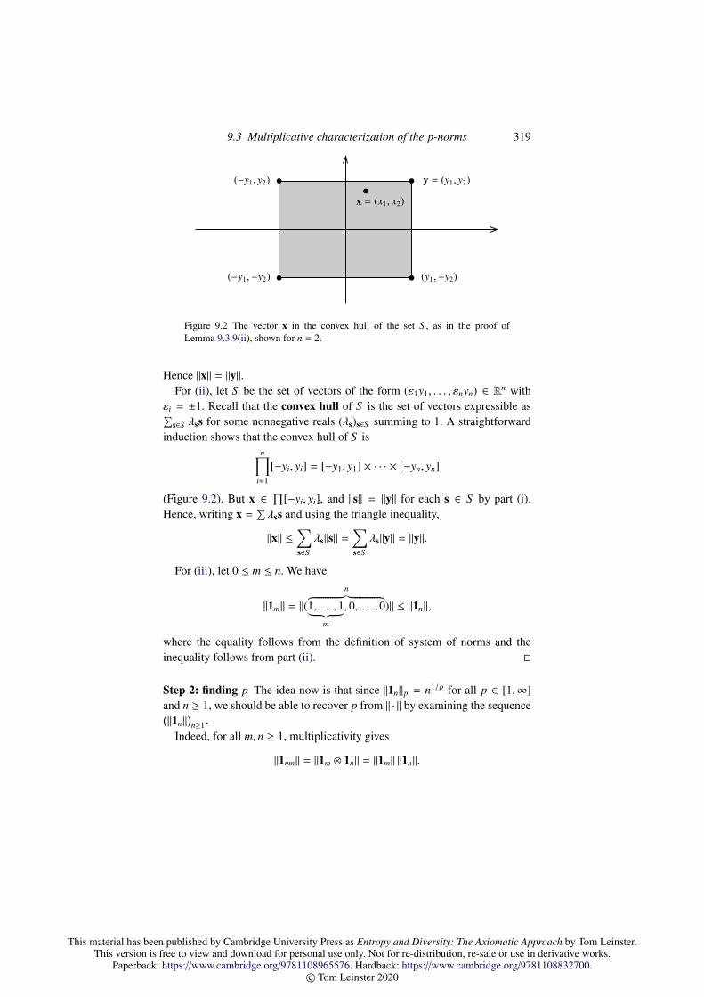
This material has been published by Cambridge University Press as Entropy and Diversity: The Axiomatic Approach by Tom Leinster.This version is free to view and download for personal use only. Not for re-distribution, re-sale or use in derivative works.
Paperback: https://www.cambridge.org/9781108965576. Hardback: https://www.cambridge.org/9781108832700.© Tom Leinster 2020
9.3 Multiplicative characterization of the p-norms 319
x = (x1, x2)
y = (y1, y2)
(y1,−y2)(−y1,−y2)
(−y1, y2)
Figure 9.2 The vector x in the convex hull of the set S , as in the proof ofLemma 9.3.9(ii), shown for n = 2.
Hence ‖x‖ = ‖y‖.For (ii), let S be the set of vectors of the form (ε1y1, . . . , εnyn) ∈ Rn with
εi = ±1. Recall that the convex hull of S is the set of vectors expressible as∑s∈S λss for some nonnegative reals (λs)s∈S summing to 1. A straightforward
induction shows that the convex hull of S isn∏
i=1
[−yi, yi] = [−y1, y1] × · · · × [−yn, yn]
(Figure 9.2). But x ∈∏
[−yi, yi], and ‖s‖ = ‖y‖ for each s ∈ S by part (i).Hence, writing x =
∑λss and using the triangle inequality,
‖x‖ ≤∑s∈S
λs‖s‖ =∑s∈S
λs‖y‖ = ‖y‖.
For (iii), let 0 ≤ m ≤ n. We have
‖1m‖ = ‖(
n︷ ︸︸ ︷1, . . . , 1︸ ︷︷ ︸
m
, 0, . . . , 0)‖ ≤ ‖1n‖,
where the equality follows from the definition of system of norms and theinequality follows from part (ii).
Step 2: finding p The idea now is that since ‖1n‖p = n1/p for all p ∈ [1,∞]and n ≥ 1, we should be able to recover p from ‖ · ‖ by examining the sequence(‖1n‖
)n≥1.
Indeed, for all m, n ≥ 1, multiplicativity gives
‖1mn‖ = ‖1m ⊗ 1n‖ = ‖1m‖ ‖1n‖.

This material has been published by Cambridge University Press as Entropy and Diversity: The Axiomatic Approach by Tom Leinster.This version is free to view and download for personal use only. Not for re-distribution, re-sale or use in derivative works.
Paperback: https://www.cambridge.org/9781108965576. Hardback: https://www.cambridge.org/9781108832700.© Tom Leinster 2020
320 Probabilistic methods
Moreover, Lemma 9.3.9(iii) implies that the sequence(‖1n‖
)n≥1 is increasing.
Hence by Theorem 1.2.1 applied to the sequence(log ‖1n‖
)n≥1, there exists
c ≥ 0 such that ‖1n‖ = nc for all n ≥ 1. Now
2c = ‖(1, 1)‖ ≤ ‖(1, 0)‖ + ‖(0, 1)‖ = 2 · ‖(1)‖ = 2 · 1c = 2,
so c ∈ [0, 1]. Put p = 1/c ∈ [1,∞]. Then
‖1n‖ = n1/p = ‖1n‖p
for all n ≥ 1.We will show that ‖x‖ = ‖x‖p for all n ≥ 0 and x ∈ Rn. By definition
of system of norms and Lemma 9.3.9(i), it is enough to prove this when x ∈(0,∞)n. The case n = 0 is trivial, so we can also restrict to n ≥ 1.
Step 3: the case p = ∞ This case needs separate handling, and is straightfor-ward anyway. We show directly that if p = ∞ (that is, if ‖1n‖ = 1 for all n ≥ 1)then ‖ · ‖ = ‖ · ‖∞.
Let x ∈ (0,∞)n, and choose j such that x j = ‖x‖∞. Then by Lemma 9.3.9(ii),
‖x‖ ≤ ‖(x j, . . . , x j)‖ = x j‖1n‖ = x j.
But also
‖x‖ ≥ ‖(0, . . . , 0︸ ︷︷ ︸j−1
, x j, 0, . . . , 0︸ ︷︷ ︸n− j
)‖ = ‖(x j)‖ = x j‖11‖ = x j.
Hence ‖x‖ = x j = ‖x‖∞, as required.So, we may assume henceforth that p ∈ [1,∞).
Step 4: exploiting the variational formula for p-norms We now use theformula for p-norms in Proposition 9.3.8: for x ∈ (0,∞)n,
‖x‖p = supu>0, r≥1
(ur N(x⊗r, ur)1/p
)1/r.
(This is where the probability theory is used, as Proposition 9.3.8 was derivedfrom the variational formula for moment generating functions.) Since m1/p =
‖1m‖ for all m, an equivalent statement is that
‖x‖p = supu>0, r≥1
∥∥∥(N(x⊗r, ur) ∗ ur)∥∥∥1/r. (9.22)
Here we have used the notation ∗ introduced after Definition 5.2.9.The expression (9.22) for ‖x‖p has the feature that it makes no mention of p.
We will use it to prove first that ‖x‖ ≥ ‖x‖p, then that ‖x‖ ≤ ‖x‖p.

This material has been published by Cambridge University Press as Entropy and Diversity: The Axiomatic Approach by Tom Leinster.This version is free to view and download for personal use only. Not for re-distribution, re-sale or use in derivative works.
Paperback: https://www.cambridge.org/9781108965576. Hardback: https://www.cambridge.org/9781108832700.© Tom Leinster 2020
9.3 Multiplicative characterization of the p-norms 321
Step 5: the lower bound Let x ∈ (0,∞)n. We show that ‖x‖ ≥ ‖x‖p. By (9.22)and multiplicativity, it is equivalent to show that
‖x⊗r‖ ≥∥∥∥(N(x⊗r, ur) ∗ ur)∥∥∥
for all real u > 0 and integers r ≥ 1. But this is clear, since by Lemma 9.3.9(ii)and the definition of system of norms,
‖x⊗r‖ ≥∥∥∥( nr︷ ︸︸ ︷
ur, . . . , ur︸ ︷︷ ︸N(x⊗r ,ur)
, 0, . . . , 0)∥∥∥ =
∥∥∥(N(x⊗r, ur) ∗ ur)∥∥∥.Step 6: the upper bound Let x ∈ (0,∞)n. We show that ‖x‖ ≤ ‖x‖p. Theargument is structurally very similar to the second part of the proof of Theo-rem 9.1.1, and uses the tensor power trick (Tao [322], Section 1.9).
Let θ ∈ (1,∞). We will prove that ‖x‖ ≤ θ‖x‖p. Since mini xi > 0, we canchoose an integer d ≥ 1 and real numbers u0, . . . , ud such that
mini
xi = u0 < u1 < · · · < ud = maxi
xi
and uk/uk−1 < θ for all k ∈ 1, . . . , d.Let r ≥ 1. We have the vector x⊗r ∈ Rnr
, and we define a new vectoryr ∈ R
nrby rounding up each coordinate of x⊗r to the next element of the
set ur1, . . . , u
rd. (Formally, define a map fr : [ur
0, urd] → [ur
0, urd] by fr(w) = ur
k,where k ∈ 1, . . . , d is least such that w ≤ ur
k. Then yr is obtained from x⊗r byapplying fr in each coordinate.)
By construction, x⊗r ≤ yr, and the number nk,r of coordinates of yr equal tour
k is at most N(x⊗r, urk−1). Hence
‖x⊗r‖ ≤ ‖yr‖ (9.23)
=∥∥∥(n1,r ∗ ur
1, . . . , nd,r ∗ urd)∥∥∥ (9.24)
≤
d∑k=1
∥∥∥((n1,r + · · · + nk−1,r) ∗ 0, nk,r ∗ urk, (nk+1,r + · · · + nd,r) ∗ 0
)∥∥∥ (9.25)
=
d∑k=1
‖(nk,r ∗ urk)‖ (9.26)
≤ d max1≤k≤d
‖(nk,r ∗ urk)‖ (9.27)
≤ dθr max1≤k≤d
‖(nk,r ∗ urk−1)‖ (9.28)
≤ dθr max1≤k≤d
∥∥∥(N(x⊗r, urk−1) ∗ ur
k−1)∥∥∥ (9.29)
≤ dθr‖x‖rp, (9.30)

This material has been published by Cambridge University Press as Entropy and Diversity: The Axiomatic Approach by Tom Leinster.This version is free to view and download for personal use only. Not for re-distribution, re-sale or use in derivative works.
Paperback: https://www.cambridge.org/9781108965576. Hardback: https://www.cambridge.org/9781108832700.© Tom Leinster 2020
322 Probabilistic methods
where (9.23) is by Lemma 9.3.9(ii), (9.24) is by symmetry and definitionof nk,r, (9.25) is by the triangle inequality, (9.26) is by definition of sys-tem of norms, (9.27) is elementary, (9.28) is by hypothesis on u0, . . . , ud andLemma 9.3.9(ii), (9.29) uses Lemma 9.3.9(iii), and (9.30) follows from (9.22).Hence by multiplicativity,
‖x‖ = ‖x⊗r‖1/r ≤ d1/rθ‖x‖p.
This holds for all integers r ≥ 1 and real numbers θ > 1. Letting r → ∞ andθ → 1 gives ‖x‖ ≤ ‖x‖p, completing the proof of Theorem 9.3.7.
Remark 9.3.10 The proof of Theorem 9.3.7 originally given by Aubrun andNechita relied on both Cramer’s theorem and the Legendre–Fenchel theorem.Effectively, they used Cramer’s theorem and convex duality to derive the mo-ment generating function formula of Theorem 9.1.1 in the specific case re-quired.
However, Cerf and Petit [62] showed how the moment generating functionformula can be proved without these tools. (In fact, they used it as part of theirproof of Cramer’s theorem.) The proof of the moment generating function for-mula given in Section 9.1 is similarly elementary. Our proof of Theorem 9.3.7works directly from the moment generating function formula, and does not,therefore, need Cramer’s theorem, the Legendre–Fenchel theorem, or even thenotion of convex conjugate.
Aubrun and Nechita went on to prove similar characterizations of the Lp
norms (Theorem 1.2 of [20]) and the Schatten p-norms (their Theorem 4.2).The main focus of the article of Fernandez-Gonzalez, Palazuelos and Perez-Garcıa [100] was also the Lp norms (their Theorem 3.1). We do not discussthese results further.
9.4 Multiplicative characterization of the power means
From the multiplicative characterization of the p-norms, we derive a multi-plicative characterization of the power means of order at least 1. It differs fromthe characterizations of power means in Section 5.5 in that it does not assumemodularity. Instead, it uses the multiplicativity condition of Definition 4.2.27,as well as a convexity axiom that provides the connection with norms.
Definition 9.4.1 A sequence of functions(M : ∆n × [0,∞)n → [0,∞)
)n≥1 is
convex if
M(p, 1
2 (x + y))≤ max
M(p, x),M(p, y)

This material has been published by Cambridge University Press as Entropy and Diversity: The Axiomatic Approach by Tom Leinster.This version is free to view and download for personal use only. Not for re-distribution, re-sale or use in derivative works.
Paperback: https://www.cambridge.org/9781108965576. Hardback: https://www.cambridge.org/9781108832700.© Tom Leinster 2020
9.4 Multiplicative characterization of the power means 323
for all n ≥ 1, p ∈ ∆n, and x, y ∈ [0,∞)n.
Example 9.4.2 The power mean Mt is multiplicative for all t ∈ [−∞,∞](Corollary 4.2.28). If t ∈ [1,∞] then Mt is also convex. To show this, it sufficesto prove the inequality in Definition 9.4.1 in the case where p has full support.In that case, Mt can be expressed in terms of ‖ · ‖t by the formula
Mt(p, x) = ‖p1/tx‖t
(x ∈ [0,∞)n), where both the power and the product of vectors are definedcoordinatewise. Now, for x, y ∈ [0,∞)n,
Mt(p, 1
2 (x + y))
=∥∥∥ 1
2 p1/tx + 12 p1/ty
∥∥∥t
≤ 12
∥∥∥p1/tx∥∥∥
t + 12
∥∥∥p1/ty∥∥∥
t
= 12(Mt(p, x) + Mt(p, y)
)≤ max
Mt(p, x),Mt(p, y)
,
by the triangle inequality for ‖ · ‖t. Thus, Mt is convex for t ∈ [1,∞].On the other hand, Mt is not convex for t ∈ [−∞, 1), since then
Mt
(( 12 ,
12), 1
2((1, 0) + (0, 1)
))= 1
2
but
maxMt
(( 12 ,
12), (1, 0)
),Mt
(( 12 ,
12), (0, 1)
)= Mt
(( 12 ,
12), (1, 0)
)=
( 1
2)1/t if t ∈ (0, 1),
0 if t ∈ [−∞, 0],
which is strictly less than 1/2.
The multiplicative characterization of the power means is as follows. For areview of the terminology used in (i), see Appendix B.
Theorem 9.4.3 Let(M : ∆n×[0,∞)n → [0,∞)
)n≥1 be a sequence of functions.
The following are equivalent:
i. M is natural, consistent, increasing, multiplicative, and convex;ii. M = Mt for some t ∈ [1,∞].
The proof follows shortly.
Remarks 9.4.4 i. We have already made some elementary inferences fromcombinations of the properties in part (i) of the theorem. In the proofof Lemma 4.2.11 (p. 107), we showed that naturality implies symmetry,absence-invariance and repetition. Since M is increasing, Lemma 5.5.3 then
This material has been published by Cambridge University Press as Entropy and Diversity: The Axiomatic Approach by Tom Leinster.This version is free to view and download for personal use only. Not for re-distribution, re-sale or use in derivative works.
Paperback: https://www.cambridge.org/9781108965576. Hardback: https://www.cambridge.org/9781108832700.© Tom Leinster 2020
324 Probabilistic methods
implies that M also has the transfer property. Moreover, M is homogeneous,since for all p ∈ ∆n, x ∈ [0,∞)n, and c ∈ [0,∞),
M(p, cx) = M(u1 ⊗ p, (c) ⊗ x
)= M
(u1, (c)
)M(p, x)
= cM(p, x),
by definition of ⊗, multiplicativity, and consistency.ii. Theorem 9.4.3 first appeared as Theorem 1.3 of Leinster [212]. There,
the result was stated with a superficially weaker consistency axiom: thatM(u1, (x)) = x for all x ∈ [0,∞). But in the presence of the naturality prop-erty, this easily implies full consistency: for naturality implies repetition (asjust noted), which in turn implies that
M(p, (x, . . . , x)
)= M
((p1 + · · · + pn), (x)
)= M
(u1, (x)
)= x
for all p ∈ ∆n and x ∈ [0,∞).
We now embark on the proof of Theorem 9.4.3. Certainly (ii) implies (i), byLemmas 4.2.14, 4.2.17 and 4.2.19, Corollary 4.2.28, and Example 9.4.2. Forthe converse, and for the rest of this section, let M be a sequence of functionssatisfying the conditions in Theorem 9.4.3(i). We will prove that M = Mt forsome t ∈ [1,∞].
Step 1: finding t The observation behind this step is that
Mt((p, 1 − p), (1, 0)
)= p1/t
for all p ∈ (0, 1).Define a function f : (0, 1)→ [0,∞) by
f (p) = M((p, 1 − p), (1, 0)
).
By multiplicativity and repetition (proved in Remark 9.4.4(i)),
f (p) f (r) = M((p, 1 − p), (1, 0)
)· M
((r, 1 − r), (1, 0)
)= M
((p, 1 − p) ⊗ (r, 1 − r), (1, 0) ⊗ (1, 0)
)= M
((pr, p(1 − r), (1 − p)r, (1 − p)(1 − r)
), (1, 0, 0, 0)
)= M
((pr, 1 − pr), (1, 0)
)= f (pr)
for all p, r ∈ (0, 1). By transfer (Remark 9.4.4(i)), f is increasing. If f (r) = 0for some r ∈ (0, 1) then for all p ∈ (0, 1),
f (p) = f (p/r) f (r) = 0 = p∞.
This material has been published by Cambridge University Press as Entropy and Diversity: The Axiomatic Approach by Tom Leinster.This version is free to view and download for personal use only. Not for re-distribution, re-sale or use in derivative works.
Paperback: https://www.cambridge.org/9781108965576. Hardback: https://www.cambridge.org/9781108832700.© Tom Leinster 2020
9.4 Multiplicative characterization of the power means 325
If not, then f defines an increasing multiplicative function (0, 1) → (0,∞), soby Corollary 1.1.16, there is some constant c ∈ [0,∞) such that f (p) = pc
for all p ∈ (0, 1). So in either case, there is a constant c ∈ [0,∞] such thatf (p) = pc for all p ∈ (0, 1). But
f( 1
2)
= M(u2, (1, 0)
)= M
(u2, (0, 1)
)by symmetry, so ( 1
2)c
= f( 1
2)
= maxM
(u2, (1, 0)
),M
(u2, (0, 1)
)≥ M
(u2,
( 12 ,
12))
= 12
by convexity and consistency. It follows that c ∈ [0, 1]. Put t = 1/c ∈ [1,∞]:then
M((p, 1 − p), (1, 0)
)= p1/t = Mt
((p, 1 − p), (1, 0)
)(9.31)
for all p ∈ (0, 1).
Step 2: constructing a system of norms Here we take our inspiration fromthe relationship
‖x‖t = n1/t Mt(un, (|x1|, . . . , |xn|)
)(x ∈ Rn) between the t-norm and the power mean of order t.
For each n ≥ 1, define a function ‖ · ‖ : Rn → [0,∞) by
‖x‖ = n1/t M(un, (|x1|, . . . , |xn|)
)(x ∈ Rn). To cover the case n = 0, let ‖ · ‖ : R0 → [0,∞) be the function whosesingle value is 0. The next few lemmas show that ‖ · ‖ is a multiplicative systemof norms.
Lemma 9.4.5 n−1/t = M(un, (1, 0, . . . , 0)
)for all n ≥ 1.
Proof By the defining property of t (equation (9.31)) and the repetition prop-erty of M, both sides are equal to M
((1/n, 1 − 1/n), (1, 0)
).
Lemma 9.4.6 For each n ≥ 0, the function ‖ · ‖ : Rn → [0,∞) is a norm.
Proof This is trivial when n = 0; suppose that n ≥ 1. We verify the threeconditions in the definition of norm (Definition 9.3.1).

This material has been published by Cambridge University Press as Entropy and Diversity: The Axiomatic Approach by Tom Leinster.This version is free to view and download for personal use only. Not for re-distribution, re-sale or use in derivative works.
Paperback: https://www.cambridge.org/9781108965576. Hardback: https://www.cambridge.org/9781108832700.© Tom Leinster 2020
326 Probabilistic methods
First, we have to prove that if 0 , x ∈ Rn then ‖x‖ , 0. We may assume bysymmetry that x1 , 0, and then
‖x‖ ≥ n1/t M(un, (|x1|, 0, . . . , 0)
)= n1/t |x1|M
(un, (1, 0, . . . , 0)
)= |x1| > 0
by definition of ‖x‖, the increasing and homogeneity properties of M, andLemma 9.4.5.
The homogeneity of M implies that ‖cx‖ = |c| ‖x‖ for all x ∈ Rn and c ∈ R.It remains to prove the triangle inequality, which we do in stages. First let
x, y ∈ Rn with ‖x‖, ‖y‖ ≤ 1 and xi, yi ≥ 0 for all i. Using the convexity of M,∥∥∥ 12 x + 1
2 y∥∥∥ = n1/t M
(un,
12 (x + y)
)≤ n1/t max
M(un, x),M(un, y)
= max
‖x‖, ‖y‖
≤ 1.
It follows that
‖λx + (1 − λ)y‖ ≤ 1 (9.32)
for all dyadic rationals λ = k/2` ∈ [0, 1], by induction on `. We now showthat (9.32) holds for all λ ∈ [0, 1]. Indeed, given λ ∈ [0, 1] and ε > 0, we canchoose a dyadic rational λ′ ∈ [0, 1] such that
λ ≤ (1 + ε)λ′, 1 − λ ≤ (1 + ε)(1 − λ′),
and then
‖λx + (1 − λ)y‖ ≤ ‖(1 + ε)λ′x + (1 + ε)(1 − λ′)y‖= (1 + ε)‖λ′x + (1 − λ′)y‖≤ 1 + ε,
where in the first inequality, we used the assumptions that M is increasing andxi, yi ≥ 0. This holds for all ε > 0, proving the claimed inequality (9.32).
Now take any x, y ∈ Rn with xi, yi ≥ 0 for all i. We will prove that
‖x + y‖ ≤ ‖x‖ + ‖y‖. (9.33)
This is immediate if x = 0 or y = 0. Supposing otherwise, put
x =x‖x‖
, y =y‖y‖
, λ =‖x‖
‖x‖ + ‖y‖.

This material has been published by Cambridge University Press as Entropy and Diversity: The Axiomatic Approach by Tom Leinster.This version is free to view and download for personal use only. Not for re-distribution, re-sale or use in derivative works.
Paperback: https://www.cambridge.org/9781108965576. Hardback: https://www.cambridge.org/9781108832700.© Tom Leinster 2020
9.4 Multiplicative characterization of the power means 327
Then ‖x‖ = ‖y‖ = 1, so by inequality (9.32) applied to x, y and λ,
‖x + y‖ = (‖x‖ + ‖y‖) ‖λx + (1 − λ)y‖ ≤ ‖x‖ + ‖y‖.
Finally, take any x, y ∈ Rn. To prove the triangle inequality (9.33), put x′ =
(|x1|, . . . , |xn|) and y′ = (|y1|, . . . , |yn|). Then ‖x‖ = ‖x′‖ and ‖y‖ = ‖y′‖ bydefinition of ‖ · ‖, and
‖x + y‖ ≤ ‖x′ + y′‖
since M is increasing. By the inequality proved in the previous paragraph,
‖x′ + y′‖ ≤ ‖x′‖ + ‖y′‖,
and the triangle inequality (9.33) follows.
Lemma 9.4.7 ‖ · ‖ is a multiplicative system of norms.
Proof We have just shown that ‖ · ‖ is a norm on Rn for each individual n.Symmetry of M implies symmetry of ‖ · ‖, so to show that ‖ · ‖ is a system ofnorms, it suffices to prove that
‖(x1, . . . , xn)‖ = ‖(x1, . . . , xn, 0)‖ (9.34)
for all n ≥ 1 and x ∈ Rn. By definition of ‖·‖ and Lemma 9.4.5, equation (9.34)is equivalent to
M(un, (|x1|, . . . , |xn|)
)M
(un, (1, 0, . . . , 0)
) =M
(un+1, (|x1|, . . . , |xn|, 0)
)M
(un+1, (1, 0, . . . , 0, 0)
) ,or equivalently,
M(un+1, (1, 0, . . . , 0, 0)
)· M
(un, (|x1|, . . . , |xn|)
)= M
(un, (1, 0, . . . , 0)
)· M
(un+1, (|x1|, . . . , |xn|, 0)
).
But by multiplicativity and symmetry, both sides are equal to
M(un(n+1), (|x1|, . . . , |xn|, 0, . . . , 0︸ ︷︷ ︸
n2
)),
proving (9.34).Finally, the system of norms ‖ ·‖ is multiplicative, by multiplicativity of M.
Step 3: using the norm theorem It now follows from Theorem 9.3.7 that‖ · ‖ = ‖ · ‖s for some s ∈ [1,∞]. Thus, ‖x‖s = n1/t M(un, x) for all n ≥ 1 andx ∈ [0,∞)n. But also, ‖x‖s = n1/sMs(un, x), so
n1/t M(un, x) = n1/sMs(un, x)

This material has been published by Cambridge University Press as Entropy and Diversity: The Axiomatic Approach by Tom Leinster.This version is free to view and download for personal use only. Not for re-distribution, re-sale or use in derivative works.
Paperback: https://www.cambridge.org/9781108965576. Hardback: https://www.cambridge.org/9781108832700.© Tom Leinster 2020
328 Probabilistic methods
for all n ≥ 1 and x ∈ [0,∞). Putting n = 2 and x = (1, 1), and using theconsistency of both M and Ms, gives s = t. Hence for all n ≥ 1 and x ∈ [0,∞)n,
M(un, x) = Mt(un, x).
Step 4: arbitrary weights We have now shown that M(un,−) = Mt(un,−) forall n ≥ 1. To extend the equality to arbitrary weights, we use Proposition 5.5.7,taking M′ = Mt there. The hypotheses of that proposition are satisfied, byRemark 9.4.4(i) and Lemma 4.2.6(i). Hence M = Mt.
This completes the proof of Theorem 9.4.3, the multiplicative characteriza-tion of the power means.
This material has been published by Cambridge University Press as Entropy and Diversity: The Axiomatic Approach by Tom Leinster.This version is free to view and download for personal use only. Not for re-distribution, re-sale or use in derivative works.
Paperback: https://www.cambridge.org/9781108965576. Hardback: https://www.cambridge.org/9781108832700.© Tom Leinster 2020
10
Information loss
Grothendieck came along and said, ‘No, the Riemann–Roch theorem isnot a theorem about varieties, it’s a theorem about morphisms betweenvarieties.’ – Nicholas Katz (quoted in [152], p. 1046).
This short chapter tells the following story. A measure-preserving map be-tween finite probability spaces can be regarded as a deterministic process. Assuch, it loses information. We can attempt to quantify how much informationis lost. It turns out that as soon as we impose a few reasonable requirementson this quantity, it is highly constrained: up to a constant factor, it must be thedifference between the entropies of the domain and the codomain. That is ourmain theorem.
This result is essentially another characterization of Shannon entropy, andfirst appeared in a 2011 paper of Baez, Fritz and Leinster [25]. The broad ideais to shift the focus from objects (finite probability spaces) to maps betweenobjects (measure-preserving maps). Entropy is an invariant of finite probabil-ity spaces; information loss is an invariant of measure-preserving maps. Theshift of emphasis from objects to maps is integral to category theory, and hasborne fruit such as the Grothendieck–Riemann–Roch theorem alluded to in theopening quotation, as well as the considerably more humble characterizationof information loss described here.
In full categorical generality, a map Xf−→ Y of any kind can be viewed
as an object X parametrized by another object Y. An object X can be viewed
as a map of a special kind, namely, the unique map X!X−→ 1 to the terminal
object 1 of the category concerned. In the case at hand, we associate with any
probability space X the unique measure-preserving map X!X−→ 1 to the one-
point space 1, and the information loss of the map !X is equal to the entropy ofthe space X. Thus, entropy is a special case of information loss.
An advantage of working with information loss rather than entropy (that is,
329
This material has been published by Cambridge University Press as Entropy and Diversity: The Axiomatic Approach by Tom Leinster.This version is free to view and download for personal use only. Not for re-distribution, re-sale or use in derivative works.
Paperback: https://www.cambridge.org/9781108965576. Hardback: https://www.cambridge.org/9781108832700.© Tom Leinster 2020
330 Information loss
maps rather than objects) is that the characterization theorems take on a newsimplicity. For instance, the conditions in our main result (Theorem 10.2.1)look just like the linearity or homomorphism conditions that appear throughoutmathematics. In contrast, the chain rule for entropy, while justifiable in manyother ways, has a more complicated algebraic form.
We begin with a review of measure-preserving maps, then define informa-tion loss (Section 10.1). After recording a few simple properties of informa-tion loss, we prove that they characterize it uniquely (Section 10.2). An analo-gous and even simpler result is then proved for q-logarithmic information loss(q , 1). Both of these theorems first appeared in the 2011 paper of Baez, Fritzand Leinster [25].
10.1 Measure-preserving maps
So far in this text, we have focused on probability distributions on finite setsof the special form 1, . . . , n. Here, it is convenient to use arbitrary finite sets.The difference is cosmetic, but does cause some shifts in notation, as follows.
Definition 10.1.1 i. Let X be a finite set. A probability distribution p on Xis a family (pi)i∈X of nonnegative real numbers such that
∑i∈X pi = 1. We
write ∆X for the set of probability distributions on X.ii. A finite probability space is a pair (X,p) whereX is a finite set and p ∈ ∆X.
The set ∆X is topologized as a subspace of the product space RX.
Definition 10.1.2 Let (Y, s) and (X,p) be finite probability spaces. Ameasure-preserving map (Y, s)→ (X,p) is a function f : Y → X such that
pi =∑
j∈ f −1(i)
s j (10.1)
for all i ∈ X.
An equivalent statement is that f : (Y, s) → (X,p) is measure-preserving ifand only if ∑
i∈V
pi =∑
j∈ f −1V
s j (10.2)
for all V ⊆ X. Indeed, (10.1) is the case of (10.2) where V = i, and (10.2)follows from (10.1) by summing over all i ∈ V.
Remarks 10.1.3 i. For any finite probability space (Y, s) and function f fromY to another finite set X, there is an induced probability distribution f s on

This material has been published by Cambridge University Press as Entropy and Diversity: The Axiomatic Approach by Tom Leinster.This version is free to view and download for personal use only. Not for re-distribution, re-sale or use in derivative works.
Paperback: https://www.cambridge.org/9781108965576. Hardback: https://www.cambridge.org/9781108832700.© Tom Leinster 2020
10.1 Measure-preserving maps 331
X, the pushforward of s along f . It is defined by the obvious generalizationof Definition 2.1.10:
( f s)i =∑
j∈ f −1(i)
s j
(i ∈ X). In these terms, a function f : (Y, s)→ (X,p) is measure-preservingif and only if f s = p.
ii. Finite probability spaces and measure-preserving maps form a categoryFinProb. We note in passing that by (i), the forgetful functor FinProb →FinSet is a discrete opfibration. In fact, FinProb is the category of elementsof the functor FinSet→ Set defined on objects byX 7→ ∆X and on maps bypushforward. (For the categorical terminology used here, see for instanceRiehl [294], Definition 2.4.1 and Exercise 2.4.viii.)
Although a measure-preserving map need not be literally surjective, it isessentially so, in the sense that all elements not in the image have probabilityzero.
Example 10.1.4 Let Y = a, a, a, b, c, c, . . . be the set of symbols in theFrench language, and let s ∈ ∆Y be their frequency distribution (as in Ex-ample 2.1.5). Let X = a, b, c, . . . be the 26-element set of letters, and p ∈ ∆X
their frequency distribution. There is a function f : Y → X that forgets ac-cents; for instance, f (a) = f (a) = f (a) = a. Then f : (Y, s) → (X,p) ismeasure-preserving and surjective.
Example 10.1.5 Let ` be the inclusion function 1 → 1, 2. Give 1 itsunique probability distribution (1) = u1, and give 1, 2 the distribution (1, 0).Then ` is measure-preserving but not surjective.
Any measure-preserving map between finite probability spaces can be fac-torized canonically into maps of the two types in these two examples: a sur-jection followed by a subset inclusion, where the subset concerned has totalprobability 1. Specifically, f : (Y, s)→ (X,p) factorizes as
(Y, s)f ′−→ ( fY,p′)
`−→ (X,p),
where p′ is the probability distribution on fY defined by p′i = pi for all i ∈ fY,the surjection f ′ is defined by f ′( j) = f ( j) for all j ∈ Y, and ` is inclusion.
A measure-preserving surjection simply discards information (such as theaccents in Example 10.1.4). It is a coarse-graining, in the sense of taking finely-grained information (such as letters with accents) and converting it into morecoarsely-grained information (such as mere letters). A measure-preserving in-clusion is essentially trivial, simply appending some events of probability zero.
This material has been published by Cambridge University Press as Entropy and Diversity: The Axiomatic Approach by Tom Leinster.This version is free to view and download for personal use only. Not for re-distribution, re-sale or use in derivative works.
Paperback: https://www.cambridge.org/9781108965576. Hardback: https://www.cambridge.org/9781108832700.© Tom Leinster 2020
332 Information loss
For any measure-preserving bijection f : (Y, s) → (X,p) between finiteprobability spaces, the inverse f −1 is also measure-preserving. We call suchan f an isomorphism, and write (Y, s) (X,p).
An important feature of probability spaces is that we can take con-vex combinations of them. Given w ∈ ∆n and finite probability spaces(X1,p1), . . . , (Xn,pn), we obtain a new probability space( n∐
i=1
Xi,
n∐i=1
wipi),
where∐Xi is the disjoint union of sets X1 t · · · t Xn and
∐wipi is the prob-
ability distribution on∐Xi that gives probability wi pi
j to an element j ∈ Xi.Convex combination of probability spaces is just composition of probability
distributions, translated into different notation. More exactly, ifXi = 1, . . . , ki
then∐Xi is in canonical bijection with 1, . . . , k1 + · · · + kn, and under this
bijection,∐
wipi corresponds to the composite distribution w (p1, . . . ,pn).The construction of convex combinations is functorial, that is, applies
not only to probability spaces but also to maps between them. Indeed, takemeasure-preserving maps
(Y1, s1)f1−→ (X1,p1)...
...
(Yn, sn)fn−→ (Xn,pn)
between finite probability spaces, and a probability distribution w ∈ ∆n. Thereis a function
n∐i=1
Yi
n∐i=1
fi//
n∐i=1
Xi
that maps j ∈ Yi to fi( j) ∈ Xi, and it is easily checked that∐
fi is a measure-preserving map
( n∐i=1
Yi,
n∐i=1
wisi) n∐
i=1fi//( n∐
i=1
Xi,
n∐i=1
wipi). (10.3)
It will be convenient to use the alternative notationn∐
i=1
wi fi or w1 f1 t · · · t wn fn
for the measure-preserving map∐n
i=1 fi of (10.3).

This material has been published by Cambridge University Press as Entropy and Diversity: The Axiomatic Approach by Tom Leinster.This version is free to view and download for personal use only. Not for re-distribution, re-sale or use in derivative works.
Paperback: https://www.cambridge.org/9781108965576. Hardback: https://www.cambridge.org/9781108832700.© Tom Leinster 2020
10.1 Measure-preserving maps 333
We defined Shannon entropy only for probability distributions on sets ofthe form 1, . . . , n, but, of course, the definition for general finite probabilityspaces (X,p) is
H(p) = −∑
i∈supp(p)
pi log pi,
where supp(p) = i ∈ X : pi > 0. Shannon entropy is isomorphism-invariant, meaning that H(p) = H(s) whenever (X,p) and (Y, s) are isomor-phic finite probability spaces.
Translated into this notation, the chain rule for Shannon entropy states that
H( n∐
i=1
wipi)
= H(w) +
n∑i=1
wiH(pi) (10.4)
for all w ∈ ∆n and finite probability spaces (X1,p1), . . . , (Xn,pn). The continu-ity property of entropy is that for each finite set X, the function
∆X → R
p 7→ H(p)(10.5)
is continuous.We now set out to quantify the information lost by a measure-preserving
map f , first exploring through examples how a reasonable definition of infor-mation loss ought to behave.
Example 10.1.6 If f is an isomorphism then f should lose no information atall. More generally, the same should be true if f is injective.
Example 10.1.7 The unique measure-preserving map (1, 2,u2) → (1,u1)forgets the result of a fair coin toss. Intuitively, then, it loses one bit of infor-mation.
Example 10.1.8 More generally, for any finite probability space (X,p), con-sider the unique measure-preserving map
f : (X,p)→(1,u1
),
which forgets the result of an observation drawn from the distribution p.Such an observation contains H(2)(p) bits of information (in the sense of Sec-tion 2.3), so the information lost by f should be H(2)(p) bits.
Example 10.1.9 Suppose that I draw fairly from a pack of playing cards, andtell you only the rank (number) of the card chosen. The information that Iam withholding is the suit, which needs log2 4 = 2 bits to encode. Thus, iff : Y → X is a four-to-one map from a 52-element set Y to a 13-element set

This material has been published by Cambridge University Press as Entropy and Diversity: The Axiomatic Approach by Tom Leinster.This version is free to view and download for personal use only. Not for re-distribution, re-sale or use in derivative works.
Paperback: https://www.cambridge.org/9781108965576. Hardback: https://www.cambridge.org/9781108832700.© Tom Leinster 2020
334 Information loss
X, and if we equip Y and X with their uniform distributions uY and uX, thenthe information loss of the measure-preserving map f : (Y,uY) → (X,uX)should be 2 bits.
Example 10.1.10 Take the measure-preserving map
f :(a, a, a, b, . . ., s
)→
(a, b, . . .,p
)of Example 10.1.4, representing the process of forgetting the accent on a letterin the French language. There are two quantities that we could reasonably callthe ‘amount of information lost’ by the process f .
First, we could condition on the underlying letter. To do this, we go throughthe 26 letters, we take for each letter the amount of information lost by forget-ting the accent on that letter, and we form the weighted mean. Write
r1 ∈ ∆3, r2 ∈ ∆1, . . . , r26 ∈ ∆1
for the accent distributions on each letter, so that s =∐26
i=1 piri. As in Exam-ple 10.1.8, the amount of information lost by forgetting the accent on an a (forinstance) should be H(2)(r1) bits. So, the expected amount of information lostby forgetting the accent on a random letter should be
26∑i=1
piH(2)(ri). (10.6)
This is one possible definition of the amount of information lost by f .Alternatively, we could define the information loss to be the amount of in-
formation we had at the start of the process minus the amount of informationthat remains at the end. This is
H(2)(s) − H(2)(p). (10.7)
But since s =∐
piri, the chain rule (10.4) tells us that the two quantities (10.6)and (10.7) are equal. So, our two ways of quantifying information loss areequivalent.
Motivated by these examples, we make the following definition.
Definition 10.1.11 Let
f : (Y, s)→ (X,p)
be a measure-preserving map of finite probability spaces. The informationloss of f is
L( f ) = H(s) − H(p).

This material has been published by Cambridge University Press as Entropy and Diversity: The Axiomatic Approach by Tom Leinster.This version is free to view and download for personal use only. Not for re-distribution, re-sale or use in derivative works.
Paperback: https://www.cambridge.org/9781108965576. Hardback: https://www.cambridge.org/9781108832700.© Tom Leinster 2020
10.1 Measure-preserving maps 335
As with other entropic quantities that we have encountered, the definition ofinformation loss depends on a choice of logarithmic base, and changing thatbase scales the quantity by a constant factor.
A deterministic process cannot create new information, and correspond-ingly, information loss is always nonnegative:
Lemma 10.1.12 Let f : (Y, s)→ (X,p) be a measure-preserving map of finiteprobability spaces. Then:
i. L( f ) =∑
j∈supp(s)
s j logp f ( j)
s j;
ii. L( f ) ≥ 0.
Proof By definition of measure-preserving map (Definition 10.1.2), p f ( j) ≥ s j
for all j ∈ Y. It follows that
j ∈ supp(s) =⇒ f ( j) ∈ supp(p). (10.8)
It also follows that log(p f ( j)/s j) ≥ 0 for all j ∈ supp(s), so part (ii) will followonce we have proved (i).
To prove (i), first note that by definition of measure-preserving map,
H(p) =∑
i∈supp(p)
pi log1pi
=∑
i∈supp(p), j∈Y : f ( j)=i
s j log1pi
=∑
j : f ( j)∈supp(p)
s j log1
p f ( j).
By (10.8), this sum is unchanged if we take j to range over supp(s) instead.Hence
L( f ) = H(s) − H(p)
=∑
j∈supp(s)
s j log1s j−
∑j∈supp(s)
s j log1
p f ( j)
=∑
j∈supp(s)
s j logp f ( j)
s j,
as claimed.
Remark 10.1.13 This result is also an instance of Lemma 8.1.3(i) on condi-tional entropy, as follows. Let V be a random variable taking values inY, with

This material has been published by Cambridge University Press as Entropy and Diversity: The Axiomatic Approach by Tom Leinster.This version is free to view and download for personal use only. Not for re-distribution, re-sale or use in derivative works.
Paperback: https://www.cambridge.org/9781108965576. Hardback: https://www.cambridge.org/9781108832700.© Tom Leinster 2020
336 Information loss
distribution s. Put U = f (V), which is a random variable taking values in X,with distribution f s = p. Then U is determined by V , so by Example 8.1.4(iv),
0 ≤ H(V | U) = H(V) − H(U) = H(s) − H(p) = L( f ).
On the other hand, by Lemma 8.1.3(i),
H(V | U) =∑
j,i : Pr( j,i)>0
Pr( j, i) logPr(i)
Pr( j, i)=
∑j : s j>0
s j logp f ( j)
s j.
Comparing the two expressions for H(V | U) gives another proof ofLemma 10.1.12.
This argument shows that information loss is a special case of conditionalentropy. But conditional entropy is also a special case of information loss.Indeed, let U and V be random variables with the same sample space, takingvalues in finite sets X andY respectively. Equip X×Y with the distribution of(U,V) and X with the distribution of U. Then the projection map
pr1 : X ×Y → X
(i, j) 7→ i
is measure-preserving. By definition, its information loss is
L(pr1) = H(U,V) − H(U) = H(V | U).
Hence H(V | U) = L(pr1), expressing conditional entropy in terms of informa-tion loss.
10.2 Characterization of information loss
In this section, we prove that information loss is uniquely characterized (up toa constant factor) by four basic properties.
First, a reversible process loses no information: L( f ) = 0 for all iso-morphisms f . This follows from the definition of L and the isomorphism-invariance of H.
Second, the amount of information lost by two processes in series is the sumof the amounts of information lost by each individually. Formally,
L(g f ) = L(g) + L( f ) (10.9)
whenever
(Y, s)f−→ (X,p)
g−→ (W, t)
This material has been published by Cambridge University Press as Entropy and Diversity: The Axiomatic Approach by Tom Leinster.This version is free to view and download for personal use only. Not for re-distribution, re-sale or use in derivative works.
Paperback: https://www.cambridge.org/9781108965576. Hardback: https://www.cambridge.org/9781108832700.© Tom Leinster 2020
10.2 Characterization of information loss 337
are measure-preserving maps of finite probability spaces. This is immediatefrom the definition of information loss.
Third, given n measure-preserving maps
(Y1, s1)f1−→ (X1,p1)...
...
(Yn, sn)fn−→ (Xn,pn)
and a distribution w ∈ ∆n, the amount of information lost by the convex com-bination
∐wi fi is given by
L( n∐
i=1
wi fi
)=
n∑i=1
wiL( fi). (10.10)
This follows from the chain rule (10.4):
L(∐
wi fi)
= H(∐
wisi)− H
(∐wipi
)=
H(w) +
∑wiH(si)
−
H(w) +
∑wiH(pi)
=
∑wiL( fi).
In particular, given measure-preserving maps
(Y, s)f−→ (X,p),
(Y′, s′)f ′−→ (X′,p′)
and a constant λ ∈ [0, 1],
L(λ f t (1 − λ) f ′
)= λL( f ) + (1 − λ)L( f ′).
Intuitively, this means that if we flip a probability-λ coin and, depending on theoutcome, do either the process f or the process f ′, then the expected informa-tion loss is λ times the information loss of f plus 1 − λ times the informationloss of f ′. So, while the previous property of L (equation (10.9)) concerned theinformation lost by two processes in series, this property (equation (10.10))concerns the information lost by two or more processes in parallel.
Fourth and finally, information loss is continuous, in the following sense. Letf : Y → X be a map of finite sets. For each probability distribution s onY, wehave the pushforward distribution f s onX, and f defines a measure-preservingmap
f : (Y, s)→ (X, f s)

This material has been published by Cambridge University Press as Entropy and Diversity: The Axiomatic Approach by Tom Leinster.This version is free to view and download for personal use only. Not for re-distribution, re-sale or use in derivative works.
Paperback: https://www.cambridge.org/9781108965576. Hardback: https://www.cambridge.org/9781108832700.© Tom Leinster 2020
338 Information loss
(Remark 10.1.3(i)). The statement is that the map
∆Y → R
s 7→ L((Y, s)
f−→ (X, f s)
)is continuous. This follows from the fact that all the maps in the (noncommu-tative) triangle
∆Ys7→ f s //
H
∆X
H~~R
are continuous.An equivalent way to state continuity is as follows. Let us say that an infinite
sequence ((Ym, sm)
fm−→ (Xm,pm)
)m≥1
of measure-preserving maps of finite probability spaces converges to a map
(Y, s)f−→ (X,p)
if (Ym
fm−→ Xm
)=
(Y
f−→ X
)for all sufficiently large m, and sm → s and pm → p as m→ ∞. Then continuityof L is equivalent to the statement that for any such convergent sequence,
L((Ym, sm)
fm−→ (Xm,pm)
)→ L
((Y, s)
f−→ (X,p)
)as m→ ∞.
The equivalence between these two formulations of continuity follows fromthe elementary fact that a map of metrizable spaces is continuous if and onlyif it preserves convergence of sequences.
We now state the main theorem, which first appeared as Theorem 2 of Baez,Fritz and Leinster [25].
Theorem 10.2.1 (Baez, Fritz and Leinster) Let K be a function assigninga real number K( f ) to each measure-preserving map f of finite probabilityspaces. The following are equivalent:
i. K has these four properties:
a. K( f ) = 0 for all isomorphisms f ;b. K(g f ) = K(g) + K( f ) for all composable pairs ( f , g) of measure-
preserving maps;

This material has been published by Cambridge University Press as Entropy and Diversity: The Axiomatic Approach by Tom Leinster.This version is free to view and download for personal use only. Not for re-distribution, re-sale or use in derivative works.
Paperback: https://www.cambridge.org/9781108965576. Hardback: https://www.cambridge.org/9781108832700.© Tom Leinster 2020
10.2 Characterization of information loss 339
c. K(λ f t (1 − λ) f ′
)= λK( f ) + (1 − λ)K( f ′) for all measure-preserving
maps f and f ′ and all λ ∈ [0, 1];d. K is continuous;
ii. K = cL for some c ∈ R.
The proof, given below, will use a version of Faddeev’s theorem:
Theorem 10.2.2 (Faddeev, version 2) Let I be a function assigning a realnumber I(p) to each finite probability space (X,p). The following are equiva-lent:
i. I is isomorphism-invariant, satisfies the chain rule (10.4), and is continuousin the sense of (10.5) (with I in place of H);
ii. I = cH for some c ∈ R.
Proof We have already observed that H satisfies the conditions in (i), and itfollows that (ii) implies (i).
Conversely, take a function I satisfying (i). Restricting I to finite sets of theform 1, . . . , n defines, for each n ≥ 1, a continuous function I : ∆n → R
satisfying the chain rule. Hence by Faddeev’s Theorem 2.5.1, there is someconstant c ∈ R such that I(p) = cH(p) for all n ≥ 1 and p ∈ ∆n. Next, take anyfinite probability space (Y, s). We have
(Y, s) (1, . . . , n,p
)for some n ≥ 1 and p ∈ ∆n, and then by isomorphism-invariance of both I andH,
I(s) = I(p) = cH(p) = cH(s),
as required.
Remark 10.2.3 The version of Faddeev’s theorem just stated is slightlyweaker than the earlier version, Theorem 2.5.1. To see this, take p ∈ ∆n and apermutation σ of 1, . . . , n. Then σ defines a measure-preserving bijection
σ :(1, . . . , n,pσ
)→
(1, . . . , n,p
).
In Theorem 10.2.2, therefore, the isomorphism-invariance axiom on I includesas a special case that I(pσ) = I(p) for all p ∈ ∆n and permutations σ. Thisis the symmetryaxiom that is traditionally included in statements of Faddeev’stheorem, but is not in fact necessary, as observed in Remark 2.5.2(ii). So, The-orem 10.2.2 is a restatement of that traditional, weaker form of Faddeev’s the-orem. The analogous restatement of the stronger Theorem 2.5.1 would involveordered probability spaces.
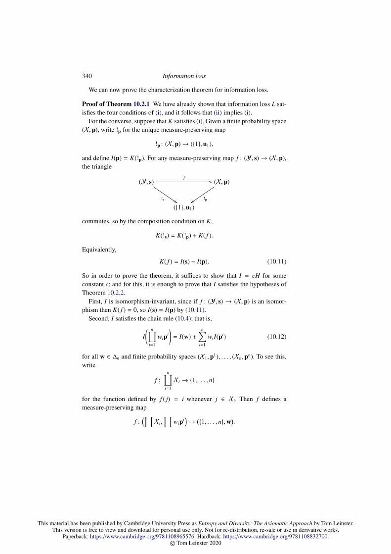
This material has been published by Cambridge University Press as Entropy and Diversity: The Axiomatic Approach by Tom Leinster.This version is free to view and download for personal use only. Not for re-distribution, re-sale or use in derivative works.
Paperback: https://www.cambridge.org/9781108965576. Hardback: https://www.cambridge.org/9781108832700.© Tom Leinster 2020
340 Information loss
We can now prove the characterization theorem for information loss.
Proof of Theorem 10.2.1 We have already shown that information loss L sat-isfies the four conditions of (i), and it follows that (ii) implies (i).
For the converse, suppose that K satisfies (i). Given a finite probability space(X,p), write !p for the unique measure-preserving map
!p : (X,p)→ (1,u1),
and define I(p) = K(!p). For any measure-preserving map f : (Y, s) → (X,p),the triangle
(Y, s)f //
!s $$
(X,p)
!pzz(1,u1)
commutes, so by the composition condition on K,
K(!s) = K(!p) + K( f ).
Equivalently,
K( f ) = I(s) − I(p). (10.11)
So in order to prove the theorem, it suffices to show that I = cH for someconstant c; and for this, it is enough to prove that I satisfies the hypotheses ofTheorem 10.2.2.
First, I is isomorphism-invariant, since if f : (Y, s) → (X,p) is an isomor-phism then K( f ) = 0, so I(s) = I(p) by (10.11).
Second, I satisfies the chain rule (10.4); that is,
I( n∐
i=1
wipi)
= I(w) +
n∑i=1
wiI(pi) (10.12)
for all w ∈ ∆n and finite probability spaces (X1,p1), . . . , (Xn,pn). To see this,write
f :n∐
i=1
Xi → 1, . . . , n
for the function defined by f ( j) = i whenever j ∈ Xi. Then f defines ameasure-preserving map
f :(∐Xi,
∐wipi
)→
(1, . . . , n,w
).

This material has been published by Cambridge University Press as Entropy and Diversity: The Axiomatic Approach by Tom Leinster.This version is free to view and download for personal use only. Not for re-distribution, re-sale or use in derivative works.
Paperback: https://www.cambridge.org/9781108965576. Hardback: https://www.cambridge.org/9781108832700.© Tom Leinster 2020
10.2 Characterization of information loss 341
We now evaluate K( f ) in two ways. On the one hand, by equation (10.11),
K( f ) = I(∐
wipi)− I(w).
On the other,
f =∐
wi !pi ,
so by hypothesis on K and induction,
K( f ) =∑
wiK(!pi ) =∑
wiI(pi).
Comparing the two expressions for K( f ) gives the chain rule (10.12) for I.Third and finally, for each finite set X, the function I : ∆X → R is continu-
ous, by continuity of K.Theorem 10.2.2 can therefore be applied, giving I = cH for some c ∈ R. It
follows from equation (10.11) that K = cL.
As observed in [25] (p. 1947), the charm of Theorem 10.2.1 is that the ax-ioms on the information loss function K are entirely linear. They give no hintof any special role for the function
p 7→ −p log p.
And yet, this function emerges in the conclusion.Another striking feature of Theorem 10.2.1 is that the natural conditions im-
posed on K force K( f ) to depend only on the domain and codomain of f . Thisis a consequence of condition (b) alone (on the information lost by a compositeprocess), as can be seen from the argument leading up to equation (10.11). Itis an instance of a general categorical fact: for any functor K from a categoryP with a terminal object to a groupoid, K( f ) = K( f ′) whenever f and f ′ aremaps in P with the same domain and the same codomain.
Theorem 10.2.1 has several variants. We can drop the condition that K( f ) =
0 for isomorphisms f if we instead require that K( f ) ≥ 0 for all f . (This wasthe version stated in Baez, Fritz and Leinster [25].) There is another version ofTheorem 10.2.1 for finite sets equipped with arbitrary finite measures insteadof probability measures (Corollary 4 of [25]). And there is a further variant forthe q-logarithmic entropies S q, which we give now.
For a measure-preserving map
f : (Y, s)→ (X,p)
between finite probability spaces, define the q-logarithmic information lossof f as
Lq( f ) = S q(s) − S q(p).

This material has been published by Cambridge University Press as Entropy and Diversity: The Axiomatic Approach by Tom Leinster.This version is free to view and download for personal use only. Not for re-distribution, re-sale or use in derivative works.
Paperback: https://www.cambridge.org/9781108965576. Hardback: https://www.cambridge.org/9781108832700.© Tom Leinster 2020
342 Information loss
The following characterization of Lq is identical to Theorem 10.2.1 except fora change in the rule for the information lost by two processes in parallel (con-dition (c) below) and the absence of a continuity condition. With some minordifferences, it first appeared as Theorem 7 of Baez, Fritz and Leinster [25].
Theorem 10.2.4 (Baez, Fritz and Leinster) Let 1 , q ∈ R. Let K be a func-tion assigning a real number K( f ) to each measure-preserving map f of finiteprobability spaces. The following are equivalent:
i. K has these three properties:
a. K( f ) = 0 for all isomorphisms f ;b. K(g f ) = K(g) + K( f ) for all composable pairs ( f , g) of measure-
preserving maps;c. K
(λ f t (1 − λ) f ′
)= λqK( f ) + (1 − λ)qK( f ′) for all measure-preserving
maps f and f ′ and all λ ∈ (0, 1);
ii. K = cLq for some c ∈ R.
No continuity or other regularity condition is needed, in contrast to Theo-rem 10.2.1.
Proof As for the proof of Theorem 10.2.1, but using the characterization the-orem for S q (Theorem 4.1.5) instead of Faddeev’s characterization of H (The-orem 2.5.1).

This material has been published by Cambridge University Press as Entropy and Diversity: The Axiomatic Approach by Tom Leinster.This version is free to view and download for personal use only. Not for re-distribution, re-sale or use in derivative works.
Paperback: https://www.cambridge.org/9781108965576. Hardback: https://www.cambridge.org/9781108832700.© Tom Leinster 2020
11
Entropy modulo a prime
Conclusion: If we have a random variable ξ which takes finitely manyvalues with all probabilities in Q then we can define not only the tran-scendental number H(ξ) but also its ‘residues modulo p’ for almost allprimes p ! – Maxim Kontsevich [193].
In this chapter, we define the entropy of any probability distribution whose‘probabilities’ are not real numbers, but integers modulo a prime p. Its en-tropy, too, is an integer mod p. We justify the definition by proving a charac-terization theorem very similar to Faddeev’s theorem on real entropy (Theo-rem 2.5.1), and by a characterization theorem for information loss mod p thatis also closely analogous to the real case.
In earlier chapters, we reached our axiomatic characterization of real infor-mation loss in three steps:
(I) characterize the sequence (log n)n≥1 (Theorem 1.2.2);(II) using (I), characterize entropy (Theorem 2.5.1);
(III) using (II), characterize information loss (Theorem 10.2.1).
Here, we follow three analogous steps to characterize entropy and informationloss modulo p (Sections 11.1 and 11.2). The analytic subtleties disappear, butinstead we encounter a number-theoretic obstacle.
With the definition of entropy mod p in place, we implement the idea pro-posed by Kontsevich in the quotation above. That is, we define a sense in whichcertain real numbers can be said to have residues mod p (Section 11.3). Theresidue map establishes a direct relationship between entropy over R and en-tropy over Z/pZ, supplementing the analogy between the Faddeev-type theo-rems over R and Z/pZ.
We finish by developing an alternative but equivalent approach to entropymodulo a prime (Section 11.4). It takes place in the ring of polynomials over
343
This material has been published by Cambridge University Press as Entropy and Diversity: The Axiomatic Approach by Tom Leinster.This version is free to view and download for personal use only. Not for re-distribution, re-sale or use in derivative works.
Paperback: https://www.cambridge.org/9781108965576. Hardback: https://www.cambridge.org/9781108832700.© Tom Leinster 2020
344 Entropy modulo a prime
the field of p elements. It is related more closely than the rest of this chapterto the subject of polylogarithms, which formed the context of Kontsevich’snote [193] and of subsequent related work such as that of Elbaz-Vincent andGangl [86, 87].
The results of this chapter first appeared in [217]. While [217] seems tohave been the first place where the theory of entropy mod p was developed indetail, many of the ideas had been sketched or at least hinted at in Kontsevich’snote [193], which itself was preceded by related work of Cathelineau [60, 61].The introduction to Elbaz-Vincent and Gangl [86] relates some of the history,including the connection with polylogarithms; see also Remark 11.4.8 below.
11.1 Fermat quotients and the definition of entropy
For the whole of this chapter, fix a prime p. To avoid confusion between theprime p and a probability distribution p, we now denote a typical probabilitydistribution by π = (π1, . . . , πn).
Our first task is to formulate the correct definition of the entropy of a prob-ability distribution π in which π1, . . . , πn are not real numbers, but elements ofthe field Z/pZ of integers modulo p.
A problem arises immediately. Real probabilities are ordinarily required tobe nonnegative, and the logarithms in the definition of entropy over Rwould beundefined if any probability were negative. So in the familiar real setting, thenotion of positivity seems to be needed in order to state a definition of entropy.But in Z/pZ, there is no sense of positive or negative. How, then, are we toimitate the definition of entropy in Z/pZ?
This problem is solved by a simple observation. Although Shannon entropyis usually only defined for sequences π = (π1, . . . , πn) of nonnegative realssumming to 1, it can just as easily be defined for sequences π of arbitrary realssumming to 1. One simply puts
H(π) = −∑
i∈supp(π)
πi log |πi|, (11.1)
where supp(π) = i : πi , 0. (See Kontsevich [193], for instance.) This ex-tended entropy is still continuous and symmetric, and still satisfies the chainrule. So, real entropy can in fact be defined without reference to the notion ofpositivity. (And generally speaking, negative probabilities are not as outlandishas they might seem; see Feynman [101] and Blass and Gurevich [42, 43].)
Thus, writing
Πn = π ∈ (Z/pZ)n : π1 + · · · + πn = 1,

This material has been published by Cambridge University Press as Entropy and Diversity: The Axiomatic Approach by Tom Leinster.This version is free to view and download for personal use only. Not for re-distribution, re-sale or use in derivative works.
Paperback: https://www.cambridge.org/9781108965576. Hardback: https://www.cambridge.org/9781108832700.© Tom Leinster 2020
11.1 Fermat quotients and the definition of entropy 345
it is reasonable to attempt to define the entropy of any element of Πn. We willrefer to elements π = (π1, . . . , πn) of Πn as probability distributions mod p, orsimply distributions. Geometrically, the set Πn of distributions on n elementsis a hyperplane in the n-dimensional vector space (Z/pZ)n over the field Z/pZ.
The function x 7→ log|x| is a homomorphism from the multiplicative groupR× of nonzero reals to the additive group R. But when we look for an analogueover Z/pZ, we run into an obstacle:
Lemma 11.1.1 There is no nontrivial homomorphism from the multiplicativegroup (Z/pZ)× of nonzero integers modulo p to the additive group Z/pZ.
Proof Let φ : (Z/pZ)× → Z/pZ be a homomorphism. The image of φ is a sub-group of Z/pZ, which by Lagrange’s theorem has order 1 or p. Since (Z/pZ)×
has order p − 1, the image of φ has order at most p − 1. It therefore has order1; that is, φ = 0.
In this sense, there is no logarithm for the integers modulo p. Nevertheless,there is an acceptable substitute. For integers n not divisible by p, Fermat’s lit-tle theorem implies that p divides np−1−1. The Fermat quotient of n modulo pis defined as
qp(n) =np−1 − 1
p∈ Z/pZ.
The resemblance between the formulas for the Fermat quotient and the q-logarithm (equation (1.17)) hints that the Fermat quotient might function assome kind of logarithm, and part (i) of the following lemma confirms that thisis so.
Lemma 11.1.2 The map qp : n ∈ Z : p - n → Z/pZ has the followingproperties:
i. qp(mn) = qp(m) + qp(n) for all m, n ∈ Z not divisible by p, and qp(1) = 0;ii. qp(n + rp) = qp(n) − r/n for all n, r ∈ Z such that n is not divisible by p;
iii. qp(n + p2) = qp(n) for all n ∈ Z not divisible by p.
Proof For (i), certainly qp(1) = 0. We now have to show that
mp−1np−1 − 1 ≡(mp−1 − 1
)+
(np−1 − 1
)(mod p2),
or equivalently, (mp−1 − 1
)(np−1 − 1
)≡ 0 (mod p2).
Since both mp−1 − 1 and np−1 − 1 are integer multiples of p, this is true.

This material has been published by Cambridge University Press as Entropy and Diversity: The Axiomatic Approach by Tom Leinster.This version is free to view and download for personal use only. Not for re-distribution, re-sale or use in derivative works.
Paperback: https://www.cambridge.org/9781108965576. Hardback: https://www.cambridge.org/9781108832700.© Tom Leinster 2020
346 Entropy modulo a prime
For (ii), we have
(n + rp)p−1 = np−1 + (p − 1)np−2rp +
p−1∑i=2
(p − 1
i
)np−i−1ri pi
≡ np−1 + p(p − 1)rnp−2 (mod p2).
Subtracting 1 from each side and dividing by p gives
qp(n + rp) ≡ qp(n) + (p − 1)rnp−2 (mod p),
and (ii) then follows from the fact that np−1 ≡ 1 (mod p). Taking r = p in (ii)gives (iii).
It follows that qp defines a group homomorphism
qp : (Z/p2Z)× → Z/pZ,
where (Z/p2Z)× is the multiplicative group of integers modulo p2. (The ele-ments of (Z/p2Z)× are the congruence classes modulo p2 of the integers notdivisible by p.) Moreover, the homomorphism qp is surjective, since the lemmaimplies that
qp(1 − rp) = qp(1) + r ≡ r (mod p)
for all integers r.Lemma 11.1.1 states that there is no logarithm mod p, in the sense that
there is no nontrivial group homomorphism (Z/pZ)× → Z/pZ. But the Fermatquotient is the next best thing, being a homomorphism (Z/p2Z)× → Z/pZ. Itis essentially the only such homomorphism:
Proposition 11.1.3 Every group homomorphism (Z/p2Z)× → Z/pZ is ascalar multiple of the Fermat quotient.
Proof It is a standard fact that the group (Z/p2Z)× is cyclic (Theorem 10.6 ofApostol [16], for instance). Choose a generator e. Since qp is surjective, it isnot identically zero, so qp(e) , 0.
Let φ : (Z/p2Z)× → Z/pZ be a group homomorphism. Put c = φ(e)/qp(e) ∈Z/pZ. Then for all n ∈ Z,
φ(en) = nφ(e) = ncqp(e) = cqp(en).
Since e is a generator, it follows that φ = cqp.
In Section 1.2, we proved characterization theorems for the sequence(log(n))n≥1. The next result plays a similar role for (qp(n))n≥1, p-n.

This material has been published by Cambridge University Press as Entropy and Diversity: The Axiomatic Approach by Tom Leinster.This version is free to view and download for personal use only. Not for re-distribution, re-sale or use in derivative works.
Paperback: https://www.cambridge.org/9781108965576. Hardback: https://www.cambridge.org/9781108832700.© Tom Leinster 2020
11.1 Fermat quotients and the definition of entropy 347
Theorem 11.1.4 Let f : n ∈ N : p - n → Z/pZ be a function. The followingare equivalent:
i. f (mn) = f (m) + f (n) and f (n + p2) = f (n) for all m, n ∈ N not divisible byp;
ii. f = cqp for some c ∈ Z/pZ.
Proof We have already shown that qp satisfies the conditions in (i), so (ii)implies (i). For the converse, suppose that f satisfies the conditions in (i).Then f induces a group homomorphism (Z/p2Z)× → Z/pZ, which by Propo-sition 11.1.3 is a scalar multiple of qp. The result follows.
In terms of the three-step plan in the introduction to this chapter, we havenow completed step (I): defining and characterizing the appropriate notion oflogarithm. We now begin step (II): defining and characterizing the appropriatenotion of entropy.
To state the definition, we will need an elementary lemma.
Lemma 11.1.5 Let a, b ∈ Z. If a ≡ b (mod p) then ap ≡ bp (mod p2).
Proof If b = a + rp with r ∈ Z, then
bp = (a + rp)p
= ap + pap−1rp +
p∑i=2
(pi
)ap−iri pi
≡ ap (mod p2).
Definition 11.1.6 Let n ≥ 1 and π ∈ Πn. The entropy of π is
H(π) =1p
(1 −
n∑i=1
api
)∈ Z/pZ,
where ai ∈ Z represents πi ∈ Z/pZ for each i ∈ 1, . . . , n.
Lemma 11.1.5 guarantees that the definition is independent of the choice ofa1, . . . , an.
We now explain and justify the definition of entropy mod p. In particular,we will prove a theorem characterizing the sequence of functions
(H : Πn →
Z/pZ)
uniquely up to a scalar multiple. This result is plainly analogous toFaddeev’s theorem for real entropy, and as such, is the strongest justificationfor the definition. But the analogy with the real case can also be seen in termsof derivations, as follows.
This material has been published by Cambridge University Press as Entropy and Diversity: The Axiomatic Approach by Tom Leinster.This version is free to view and download for personal use only. Not for re-distribution, re-sale or use in derivative works.
Paperback: https://www.cambridge.org/9781108965576. Hardback: https://www.cambridge.org/9781108832700.© Tom Leinster 2020
348 Entropy modulo a prime
The entropy of a real probability distribution π is equal to∑
i ∂(πi), where
∂(x) =
−x log x if x > 0,
0 if x = 0(11.2)
(as in Section 2.2). What is the analogue of ∂ over Z/pZ? Given the analogybetween the logarithm and the Fermat quotient, it is natural to consider −nqp(n)as a candidate. For integers n not divisible by p,
−nqp(n) =n − np
p.
The right-hand side is a well-defined integer even if n is divisible by p. Wetherefore define a map ∂ : Z→ Z/pZ by
∂(n) =n − np
p∈ Z/pZ. (11.3)
Thus,
∂(n) =
−nqp(n) if p - n,
n/p if p | n.
If n ≡ m (mod p2) then ∂(n) = ∂(m), so ∂ can also be regarded as a mapZ/p2Z → Z/pZ. Like its real counterpart, ∂ satisfies a version of the Leibnizrule (and for this reason, is essentially what is called a p-derivation [54, 55]):
Lemma 11.1.7 ∂(mn) = m∂(n) + ∂(m)n for all m, n ∈ Z.
Proof The proof is similar to that of Lemma 11.1.2(i). The statement to beproved is equivalent to
mn − mpnp ≡ m(n − np) + (m − mp)n (mod p2).
Rearranging, this in turn is equivalent to
0 ≡ (m − mp)(n − np) (mod p2),
which is true since m ≡ mp (mod p) and n ≡ np (mod p).
Using this lemma, we derive an equivalent expression for entropy mod p:
Lemma 11.1.8 For all n ≥ 1 and π ∈ Πn,
H(π) =
n∑i=1
∂(ai) − ∂( n∑
i=1
ai
),
where ai ∈ Z represents πi ∈ Z/pZ for each i ∈ 1, . . . , n.

This material has been published by Cambridge University Press as Entropy and Diversity: The Axiomatic Approach by Tom Leinster.This version is free to view and download for personal use only. Not for re-distribution, re-sale or use in derivative works.
Paperback: https://www.cambridge.org/9781108965576. Hardback: https://www.cambridge.org/9781108832700.© Tom Leinster 2020
11.1 Fermat quotients and the definition of entropy 349
Proof An equivalent statement is that
1 −∑
api ≡
∑(ai − ap
i ) −∑
ai −(∑
ai
)p
(mod p2).
Cancelling, this reduces to
1 ≡(∑
ai
)p(mod p2).
But∑πi = 1 in Z/pZ by definition of Πn, so
∑ai ≡ 1 (mod p), so
(∑ai)p≡ 1
(mod p2) by Lemma 11.1.5.
Thus, H(π) measures the extent to which the nonlinear derivation ∂ fails topreserve the sum
∑ai.
The analogy with entropy over R is now evident. For a real probability dis-tribution π, and defining ∂ : [0,∞)→ R as in equation (11.2), we also have
H(π) =∑
∂(πi) − ∂(∑
πi
).
In the real case, since∑πi = 1, the second term on the right-hand side van-
ishes. But over Z/pZ, it is not true in general that ∂(∑
ai) = 0, so it is nottrue either that H(π) =
∑∂(ai). (Indeed,
∑∂(ai), unlike H(π), depends on the
choice of representatives ai.) So in the formula
H(π) =∑
∂(ai) − ∂(∑
ai
)for entropy mod p, the second summand is indispensable.
Example 11.1.9 Let n ≥ 1 with p - n. Since n is invertible mod p, there is auniform distribution
un = (1/n, . . . , 1/n︸ ︷︷ ︸n
) ∈ Πn.
Choose a ∈ Z representing 1/n ∈ Z/pZ. By Lemma 11.1.8 and then the deriva-tion property of ∂,
H(un) = n∂(a) − ∂(na) = −a∂(n).
But ∂(n) = −nqp(n), so H(un) = qp(n). This result over Z/pZ is analogous tothe formula H(un) = log n for the real entropy of a uniform distribution.
Example 11.1.10 Let p = 2. Any distribution π ∈ Πn has an odd number ofelements in its support, since
∑πi = 1. Directly from the definition of entropy,
H(π) ∈ Z/2Z is given by
H(π) = 12(|supp(π)| − 1
)=
0 if |supp(π)| ≡ 1 (mod 4),
1 if |supp(π)| ≡ 3 (mod 4).

This material has been published by Cambridge University Press as Entropy and Diversity: The Axiomatic Approach by Tom Leinster.This version is free to view and download for personal use only. Not for re-distribution, re-sale or use in derivative works.
Paperback: https://www.cambridge.org/9781108965576. Hardback: https://www.cambridge.org/9781108832700.© Tom Leinster 2020
350 Entropy modulo a prime
In preparation for the next example, we record a useful standard lemma:
Lemma 11.1.11(
p−1s
)≡ (−1)s (mod p) for all s ∈ 0, . . . , p − 1.
Proof In Z/pZ, we have equalities(p − 1
s
)=
(p − 1)(p − 2) · · · (p − s)s!
=(−1)(−2) · · · (−s)
s!= (−1)s.
Example 11.1.12 Here we find the entropy of a distribution (π, 1 − π) on twoelements. Choose an integer a representing π ∈ Z/pZ. From the definition ofentropy, assuming that p , 2,
H(π, 1 − π) =1p(1 − ap − (1 − a)p) =
p−1∑r=1
(−1)r+1 1p
(pr
)ar.
But 1p
(pr
)= 1
r
(p−1r−1
), so by Lemma 11.1.11, the coefficient of ar in the sum is
simply 1r . We can now replace a by π, giving
H(π, 1 − π) =
p−1∑r=1
πr
r.
The function on the right-hand side was the starting point of Kontsevich’snote [193], and we return to it in Section 11.4.
In the case p = 2, we have H(π, 1 − π) = 0 for both values of π ∈ Z/2Z.
Example 11.1.13 Appending zero probabilities to a distribution does notchange its entropy:
H(π1, . . . , πn, 0, . . . , 0) = H(π1, . . . , πn).
This is immediate from the definition. But a subtlety of distributions mod p,absent in the standard real setting, is that nonzero probabilities can sum to zero.So, one might ask whether
H(π1, . . . , πn, τ1, . . . , τm) = H(π1, . . . , πn)
whenever τ1, . . . , τm ∈ Z/pZ with∑τ j = 0. The answer is trivially yes for
m = 0 and m = 1, and it is also yes for m = 2 as long as p , 2. (For if wechoose an integer a to represent τ1 then −a represents τ2, and ap + (−a)p = 0.)But the answer is no for m ≥ 3. For instance, when p = 3, we have
H(1, 1, 1, 1) = H(u4) = q3(4) = 13 (42 − 1) = −1

This material has been published by Cambridge University Press as Entropy and Diversity: The Axiomatic Approach by Tom Leinster.This version is free to view and download for personal use only. Not for re-distribution, re-sale or use in derivative works.
Paperback: https://www.cambridge.org/9781108965576. Hardback: https://www.cambridge.org/9781108832700.© Tom Leinster 2020
11.1 Fermat quotients and the definition of entropy 351
by Example 11.1.9, which is not equal to H(1) = 0, even though 1 + 1 + 1 = 0.
Distributions over Z/pZ can be composed, using the same formula as in thereal case (Definition 2.1.3). As in the real case, entropy mod p satisfies thechain rule:
Proposition 11.1.14 (Chain rule) We have
H(γ (π1, . . . ,πn)
)= H(γ) +
n∑i=1
γiH(πi)
for all n, k1, . . . , kn ≥ 1, all γ = (γ1, . . . , γn) ∈ Πn, and all πi ∈ Πki .
Proof Write πi =(πi
1, . . . , πiki
). Choose bi ∈ Z representing γi ∈ Z/pZ and
aij ∈ Z representing πi
j ∈ Z/pZ, for each i and j. Write Ai = ai1 + · · · + ai
ki.
We evaluate in turn the three terms H(γ(π1, . . . ,πn)
), H(γ), and
∑γiH(πi).
First, by Lemma 11.1.8 and the derivation property of ∂ (Lemma 11.1.7),
H(γ (π1, . . . ,πn)
)=
n∑i=1
ki∑j=1
∂(biai
j)− ∂
( n∑i=1
ki∑j=1
biaij
)
=
n∑i=1
ki∑j=1
(∂(bi)ai
j + bi∂(ai
j))− ∂
( n∑i=1
biAi)
=
n∑i=1
∂(bi)Ai +
n∑i=1
bi
ki∑j=1
∂(ai
j)− ∂
( n∑i=1
biAi).
Second, Ai ≡ 1 (mod p) since πi ∈ Πki , so biAi ∈ Z represents γi ∈ Z/pZ.Hence
H(γ) =
n∑i=1
∂(biAi) − ∂( n∑
i=1
biAi)
=
n∑i=1
∂(bi)Ai +
n∑i=1
bi∂(Ai) − ∂( n∑
i=1
biAi).
Third,n∑
i=1
γiH(πi) =
n∑i=1
bi
ki∑j=1
∂(ai
j)−
n∑i=1
bi∂(Ai).
The result follows.
There is a tensor product for distributions mod p, defined as in the real case(p. 38), and entropy mod p has the familiar logarithmic property:
Corollary 11.1.15 H(γ ⊗ π) = H(γ) + H(π) for all γ ∈ Πn and π ∈ Πm.

This material has been published by Cambridge University Press as Entropy and Diversity: The Axiomatic Approach by Tom Leinster.This version is free to view and download for personal use only. Not for re-distribution, re-sale or use in derivative works.
Paperback: https://www.cambridge.org/9781108965576. Hardback: https://www.cambridge.org/9781108832700.© Tom Leinster 2020
352 Entropy modulo a prime
11.2 Characterizations of entropy and information loss
We now state our characterization theorem for entropy mod p, whose closeresemblance to the characterization theorem for real entropy (Theorem 2.5.1)is the main justification for the definition.
Theorem 11.2.1 Let(I : Πn → Z/pZ
)n≥1 be a sequence of functions. The fol-
lowing are equivalent:
i. I satisfies the chain rule (that is, satisfies the conclusion of Proposi-tion 11.1.14 with I in place of H);
ii. I = cH for some c ∈ Z/pZ.
As in our sharper version of Faddeev’s theorem over R (Theorem 2.5.1), nosymmetry condition is needed.
Since H satisfies the chain rule, so does any constant multiple of H.Hence (ii) implies (i). We now begin the proof of the converse. For the restof the proof , let
(I : Πn → Z/pZ
)n≥1 be a sequence of functions satisfying the
chain rule.
Lemma 11.2.2 i. I(umn) = I(um) + I(un) for all m, n ∈ N not divisible by p;ii. I(u1) = 0.
Proof Both parts are proved exactly as in the real case (Lemma 2.5.3).
Lemma 11.2.3 I(1, 0) = I(0, 1) = 0.
Proof The proof that I(1, 0) = 0 is identical to the proof in the real case(Lemma 2.5.4), and I(0, 1) = 0 is proved similarly.
Lemma 11.2.4 For all π ∈ Πn and i ∈ 0, . . . , n,
I(π1, . . . , πn) = I(π1, . . . , πi, 0, πi+1, . . . , πn).
Proof First suppose that i , 0. Then
(π1, . . . , πi, 0, πi+1, . . . , πn) = π (u1, . . . ,u1︸ ︷︷ ︸
i−1
, (1, 0),u1, . . . ,u1︸ ︷︷ ︸n−i
).
Applying I to both sides, then using the chain rule and that I(u1) = I(1, 0) = 0,gives the result. The case i = 0 is proved similarly, now using I(0, 1) = 0.
As in the real case, we will prove the characterization theorem by analysingI(un) as n varies. And as in the real case, the chain rule will allow us to deducethe value of I(π) for more general distributions π:

This material has been published by Cambridge University Press as Entropy and Diversity: The Axiomatic Approach by Tom Leinster.This version is free to view and download for personal use only. Not for re-distribution, re-sale or use in derivative works.
Paperback: https://www.cambridge.org/9781108965576. Hardback: https://www.cambridge.org/9781108832700.© Tom Leinster 2020
11.2 Characterizations of entropy and information loss 353
Lemma 11.2.5 Let π ∈ Πn with πi , 0 for all i. For each i, let ki ≥ 1 be aninteger representing πi ∈ Z/pZ, and write k =
∑ni=1 ki. Then
I(π) = I(uk) −n∑
i=1
kiI(uki ).
Proof First note that none of k1, . . . , kn is a multiple of p, and since k repre-sents
∑πi = 1 ∈ Z/pZ, neither is k. Hence uki and uk are well-defined. By
definition of composition,
π (uk1 , . . . ,ukn ) = (1, . . . , 1︸ ︷︷ ︸k
) = uk.
Applying I and using the chain rule gives the result.
We now come to the most delicate part of the argument. Since H(un) =
qp(n), and since qp(n) is p2-periodic in n, if I is to be a constant multiple of Hthen I(un) must also be p2-periodic in n. We show this directly.
Lemma 11.2.6 I(un+p2 ) = I(un) for all natural numbers n not divisible by p.
Proof First we prove the existence of a constant c ∈ Z/pZ such that for alln ∈ N not divisible by p,
I(un+p) = I(un) − c/n. (11.4)
(Compare Lemma 11.1.2(ii).) An equivalent statement is that n(I(un+p)−I(un))is independent of n. For any n1 and n2, we can choose some m ≥ maxn1, n2
with m ≡ 1 (mod p), so it is enough to show that whenever 0 ≤ n ≤ m withn . 0 (mod p) and m ≡ 1 (mod p),
n(I(un+p) − I(un)
)= I(um+p) − I(um). (11.5)
To prove this, consider the distribution
π = (n, 1, . . . , 1︸ ︷︷ ︸m−n
).
By Lemma 11.2.5 and the fact that I(u1) = 0,
I(π) = I(um) − nI(un).
But also
π = (n + p, 1, . . . , 1︸ ︷︷ ︸m−n
),

This material has been published by Cambridge University Press as Entropy and Diversity: The Axiomatic Approach by Tom Leinster.This version is free to view and download for personal use only. Not for re-distribution, re-sale or use in derivative works.
Paperback: https://www.cambridge.org/9781108965576. Hardback: https://www.cambridge.org/9781108832700.© Tom Leinster 2020
354 Entropy modulo a prime
so by the same argument,
I(π) = I(um+p) − (n + p)I(un+p)
= I(um+p) − nI(un+p).
Comparing the two expressions for I(π) gives equation (11.5), thus proving theinitial claim.
By induction on equation (11.4),
I(un+rp) = I(un) − cr/n
for all n, r ∈ N with n not divisible by p. The result follows by setting r = p.
We can now prove the characterization theorem for entropy modulo p.
Proof of Theorem 11.2.1 Define f : n ∈ N : p - n → Z/pZ by f (n) =
I(un). By Lemma 11.2.2, f (mn) = f (m) + f (n) for all m, n not divisible byp. By Lemma 11.2.6, f (n + p2) = f (n) for all n not divisible by p. Hence byTheorem 11.1.4, f = cqp for some c ∈ Z/pZ. It follows from Example 11.1.9that I(un) = cH(un) for all n not divisible by p.
Since both I and cH satisfy the chain rule, Lemma 11.2.5 applies to both;and since I and cH are equal on uniform distributions, they are also equal onall distributions π such that πi , 0 for all i. Finally, applying Lemma 11.2.4 toboth I and cH, we deduce by induction that I(π) = cH(π) for all π ∈ Πn.
In the real case, the characterization theorem for entropy leads to a character-ization of information loss involving only linear conditions (Theorem 10.2.1).The same holds for entropy mod p, and the argument can be copied over fromthe real case nearly verbatim.
Thus, given a finite set X, we write ΠX for the set of families π = (πi)i∈X ofelements of Z/pZ such that
∑i∈X πi = 1. A finite probability space mod p is
a finite set X together with an element π ∈ ΠX. A measure-preserving mapf : (Y,σ)→ (X,π) between such spaces is a function f : Y → X such that
πi =∑
j∈ f −1(i)
s j
for all i ∈ X.As in the real case, we can take convex combinations of both probability
spaces and maps between them. Given two finite probability spaces mod p,say (X,π) and (X′,π′), and given also a scalar λ ∈ Z/pZ, we obtain anothersuch space,
(X t X′, λπ t (1 − λ)π′
). Given two measure-preserving maps
f : (Y,σ)→ (X,π),
f ′ : (Y′,σ′)→ (X′,π′)

This material has been published by Cambridge University Press as Entropy and Diversity: The Axiomatic Approach by Tom Leinster.This version is free to view and download for personal use only. Not for re-distribution, re-sale or use in derivative works.
Paperback: https://www.cambridge.org/9781108965576. Hardback: https://www.cambridge.org/9781108832700.© Tom Leinster 2020
11.3 The residues of real entropy 355
and an element λ ∈ Z/pZ, we obtain a new measure-preserving map
λ f t (1 − λ) f ′ :(Y tY′, λσ t (1 − λ)σ′
)→
(X t X′, λπ t (1 − λ)π′
),
exactly as in Section 10.1.The entropy of π ∈ ΠX is, naturally,
H(π) =1p
(1 −
∑i∈X
api
),
where ai ∈ Z represents πi ∈ Z/pZ for each i ∈ X. The information loss of ameasure-preserving map f : (Y,σ)→ (X,π) between finite probability spacesmod p is
L( f ) = H(σ) − H(π) ∈ Z/pZ.
Theorem 11.2.7 Let K be a function assigning an element K( f ) ∈ Z/pZ toeach measure-preserving map f of finite probability spaces mod p. The fol-lowing are equivalent:
i. K has these three properties:
a. K( f ) = 0 for all isomorphisms f ;b. K(g f ) = K(g) + K( f ) for all composable pairs ( f , g) of measure-
preserving maps;c. K
(λ f t (1 − λ) f ′
)= λK( f ) + (1 − λ)K( f ′) for all measure-preserving
maps f and f ′ and all λ ∈ Z/pZ;
ii. K = cL for some c ∈ Z/pZ.
Proof The proof is identical to that of the real case, Theorem 10.2.1, but withZ/pZ in place of R, Theorem 11.2.1 in place of Faddeev’s theorem, and allmention of continuity removed.
11.3 The residues of real entropy
Having found a satisfactory definition of the entropy of a probability distribu-tion mod p, we are now in a position to develop Kontsevich’s suggestion aboutthe residues mod p of real entropy, quoted at the start of this chapter. (Thatquotation was the sum total of what he wrote on the subject.)
Let π ∈ ∆n be a probability distribution with rational probabilities, say π =
(a1/b1, . . . , an/bn) with ai, bi ∈ Z. There are only finitely many primes thatdivide one or more of the denominators bi. If p is not in that exceptional setthen π defines an element of Πn, and therefore has a mod p entropy H(π) ∈

This material has been published by Cambridge University Press as Entropy and Diversity: The Axiomatic Approach by Tom Leinster.This version is free to view and download for personal use only. Not for re-distribution, re-sale or use in derivative works.
Paperback: https://www.cambridge.org/9781108965576. Hardback: https://www.cambridge.org/9781108832700.© Tom Leinster 2020
356 Entropy modulo a prime
Z/pZ. Kontsevich invites us to think of this as the residue class modulo p ofthe real entropy H(π) ∈ R.
Kontsevich phrased his suggestion playfully, but there is more to it thanmeets the eye. To explain it, let us write HR for entropy over the reals, Hp forentropy mod p, and ∆
(p)n for the set of real probability distributions π ∈ ∆n
such that each πi can be expressed as a rational number with denominator notdivisible by p. The proposal is that given π ∈ ∆
(p)n , we regard Hp(π) ∈ Z/pZ as
the residue mod p of HR(π) ∈ R.Now, different distributions can have the same entropy over R. For instance,
HR( 1
2 ,18 ,
18 ,
18 ,
18)
= HR( 1
4 ,14 ,
14 ,
14).
There is, therefore, a question of consistency: Kontsevich’s proposal onlymakes sense if
HR(π) = HR(γ) =⇒ Hp(π) = Hp(γ)
for all π ∈ ∆(p)n and γ ∈ ∆
(p)m . We now show that this is true.
Lemma 11.3.1 Let n,m ≥ 1 and let a1, . . . , an, b1, . . . , bm ≥ 0 be integers.Then
n∏i=1
aaii =
m∏j=1
bb j
j =⇒
n∑i=1
∂(ai) =
m∑j=1
∂(b j),
where the first equality is in Z, the second is in Z/pZ, and we use the conventionthat 00 = 1.
Here ∂ is the map Z → Z/pZ defined in equation (11.3). The analogueof this lemma for the real-valued map ∂ of equation (11.2) is trivial: simplydiscard the factors in the products for which ai or b j is 0, then take logarithms.But over Z/pZ, it is not so simple. The subtlety arises from the possibility thatsome ai or b j is not zero but is divisible by p. In that case,
∏aai
i =∏
bb j
jis divisible by p, so its Fermat quotient – the analogue of the logarithm – isundefined. A more detailed analysis is therefore required.
Proof Since 00 = 1 and ∂(0) = 0, it is enough to prove the result in the casewhere each of the integers ai and b j is strictly positive. We may then writeai = pαi Ai with αi ≥ 0 and p - Ai, and similarly b j = pβ j B j. We adopt theconvention that unless mentioned otherwise, the index i ranges over 1, . . . , nand the index j over 1, . . . ,m.
Assume that∏
aaii =
∏bb j
j . We have∏aai
i = p∑αiai
∏Aai
i

This material has been published by Cambridge University Press as Entropy and Diversity: The Axiomatic Approach by Tom Leinster.This version is free to view and download for personal use only. Not for re-distribution, re-sale or use in derivative works.
Paperback: https://www.cambridge.org/9781108965576. Hardback: https://www.cambridge.org/9781108832700.© Tom Leinster 2020
11.3 The residues of real entropy 357
with p -∏
Aaii , and similarly for
∏bb j
j . It follows that∏Aai
i =∏
Bb j
j , (11.6)∑αiai =
∑β jb j (11.7)
in Z. We consider each of these equations in turn.First, since p -
∏Aai
i , the Fermat quotient qp(∏
Aaii)
is well-defined, andthe logarithmic property of qp (Lemma 11.1.2(i)) gives
−qp
(∏Aai
i
)=
∑−aiqp(Ai).
Consider the right-hand side as an element of Z/pZ. When p | ai, the i-summand vanishes. When p - ai, the i-summand is −aiqp(ai) = ∂(ai). Hence
−qp
(∏Aai
i
)=
∑i : αi=0
∂(ai)
in Z/pZ. A similar result holds for∏
Bb j
j , so equation (11.6) gives∑i : αi=0
∂(ai) =∑
j : β j=0
∂(b j). (11.8)
Second,n∑
i=1
αiai =∑
i : αi≥1
αiai,
so p |∑αiai. Now
1p
∑αiai =
∑i : αi≥1
αi pαi−1Ai ≡∑
i : αi=1
Ai (mod p),
and if αi = 1 then Ai = ai/p = ∂(ai). A similar result holds for∑β jb j, so
equation (11.7) gives ∑i : αi=1
∂(ai) =∑
j : β j=1
∂(b j) (11.9)
in Z/pZ.Finally, for each i such that αi ≥ 2, we have p2 | ai and so ∂(ai) = 0 in Z/pZ.
The same holds for b j, so ∑i : αi≥2
∂(ai) =∑
j : β j≥2
∂(b j), (11.10)
both sides being 0. Adding equations (11.8), (11.9) and (11.10) gives the re-sult.

This material has been published by Cambridge University Press as Entropy and Diversity: The Axiomatic Approach by Tom Leinster.This version is free to view and download for personal use only. Not for re-distribution, re-sale or use in derivative works.
Paperback: https://www.cambridge.org/9781108965576. Hardback: https://www.cambridge.org/9781108832700.© Tom Leinster 2020
358 Entropy modulo a prime
We deduce that the real entropy of a rational distribution determines its en-tropy mod p:
Theorem 11.3.2 Let n,m ≥ 1, π ∈ ∆(p)n , and γ ∈ ∆
(p)m . Then
HR(π) = HR(γ) =⇒ Hp(π) = Hp(γ).
Proof We can write
π = (r1/t, . . . , rn/t), γ = (s1/t, . . . , sm/t),
where ri, s j and t are nonnegative integers such that p - t and
r1 + · · · + rn = t = s1 + · · · + sm.
By multiplying all of these integers by a constant if necessary, we may assumethat t ≡ 1 (mod p).
By definition,
e−HR(π) =∏
i
(ri/t)ri/t,
with the convention that 00 = 1. Multiplying both sides by t and then raisingto the power of t gives
tte−tHR(π) =∏
i
rrii .
By the analogous equation for γ and the assumption that HR(π) = HR(γ), itfollows that ∏
i
rrii =
∏j
ss j
j .
Lemma 11.3.1 now gives ∑i
∂(ri) =∑
j
∂(s j)
in Z/pZ. Since∑
ri = t =∑
s j, it follows that∑i
∂(ri) − ∂(∑
i
ri
)=
∑j
∂(s j) − ∂(∑
j
s j
).
But t ≡ 1 (mod p), so ri represents the element ri/t = πi of Z/pZ, so byLemma 11.1.8, the left-hand side of this equation is Hp(π). Similarly, the right-hand side is Hp(γ). Hence Hp(π) = Hp(γ).

This material has been published by Cambridge University Press as Entropy and Diversity: The Axiomatic Approach by Tom Leinster.This version is free to view and download for personal use only. Not for re-distribution, re-sale or use in derivative works.
Paperback: https://www.cambridge.org/9781108965576. Hardback: https://www.cambridge.org/9781108832700.© Tom Leinster 2020
11.4 Polynomial approach 359
It follows that Kontsevich’s residue classes of real entropies are well-defined. That is, writing
E(p) =
∞⋃n=1
HR(π) : π ∈ ∆
(p)n
⊆ R,
there is a unique map of sets
[ · ] : E(p) → Z/pZ
such that [HR(π)] = Hp(π) for all π ∈ ∆(p)n and n ≥ 1. We now show that this
map is additive, as the word ‘residue’ leads one to expect.
Proposition 11.3.3 The set E(p) is closed under addition, and the residue map
[ · ] : E(p) → Z/pZHR(π) 7→ Hp(π)
preserves addition.
Proof Let π ∈ ∆(p)n and γ ∈ ∆
(p)m . We must show that HR(π) + HR(γ) ∈ E(p) and
[HR(π) + HR(γ)] = [HR(π)] + [HR(γ)].
Evidently π ⊗ γ ∈ ∆(p)nm, so by the logarithmic property of HR,
HR(π) + HR(γ) = HR(π ⊗ γ) ∈ E(p).
Now also using the logarithmic property of Hp (Corollary 11.1.15),
[HR(π) + HR(γ)] = [HR(π ⊗ γ)]
= Hp(π ⊗ γ)
= Hp(π) + Hp(γ)
= [HR(π)] + [HR(γ)],
as required.
11.4 Polynomial approach
There is an alternative approach to entropy modulo a prime. It repairs a defectof the approach above: that in order to define the entropy of a distribution πover Z/pZ, we had to step outside Z/pZ to make arbitrary choices of integersrepresenting the probabilities πi, then show that the definition was independentof those choices. We now show how to define H(π) directly as a function ofπ1, . . . , πn.

This material has been published by Cambridge University Press as Entropy and Diversity: The Axiomatic Approach by Tom Leinster.This version is free to view and download for personal use only. Not for re-distribution, re-sale or use in derivative works.
Paperback: https://www.cambridge.org/9781108965576. Hardback: https://www.cambridge.org/9781108832700.© Tom Leinster 2020
360 Entropy modulo a prime
Inevitably, that function is a polynomial, by the classical fact that every func-tion Kn → K on a finite field K is induced by some polynomial in n variables.Indeed, there is a unique such polynomial whose degree in each variable isstrictly less than the order of the field:
Lemma 11.4.1 Let K be a finite field with q elements, let n ≥ 0, and letF : Kn → K be a function. Then there is a unique polynomial f of the form
f (x1, . . . , xn) =∑
0≤r1,...,rn<q
cr1,...,rn xr11 · · · x
rnn
(cr1,...,rn ∈ K) such that
f (π1, . . . , πn) = F(π1, . . . , πn)
for all π1, . . . , πn ∈ K.
Proof See Appendix A.9.
In particular, taking K = Z/pZ, entropy modulo p can be expressed as apolynomial of degree less than p in each variable. We now identify such apolynomial.
For each n ≥ 1, define h(x1, . . . , xn) ∈ (Z/pZ)[x1, . . . , xn] by
h(x1, . . . , xn) = −∑
0≤r1,...,rn<pr1+···+rn=p
xr11 · · · x
rnn
r1! · · · rn!.
Proposition 11.4.2 For all n ≥ 1 and (π1, . . . , πn) ∈ Πn,
H(π1, . . . , πn) = h(π1, . . . , πn).
Proof Let π1, . . . , πn ∈ Z/pZ. We will show that whenever a1, . . . , an are inte-gers representing π1, . . . , πn, then
1p
(( n∑i=1
ai
)p
−
n∑i=1
api
)(11.11)
is an integer representing h(π1, . . . , πn). The result will follow, since if π ∈ Πn
then∑πi = 1, so (
∑ai)p ≡ 1 (mod p2) by Lemma 11.1.5.
We have to prove that( n∑i=1
ai
)p
−
n∑i=1
api ≡ −p
∑0≤r1,...,rn<pr1+···+rn=p
ar11 · · · a
rnn
r1! · · · rn!(mod p2).

This material has been published by Cambridge University Press as Entropy and Diversity: The Axiomatic Approach by Tom Leinster.This version is free to view and download for personal use only. Not for re-distribution, re-sale or use in derivative works.
Paperback: https://www.cambridge.org/9781108965576. Hardback: https://www.cambridge.org/9781108832700.© Tom Leinster 2020
11.4 Polynomial approach 361
Since (p − 1)! is invertible in Z/p2Z, an equivalent statement is that
(p − 1)!( n∑
i=1
api −
( n∑i=1
ai
)p)≡
∑0≤r1,...,rn<pr1+···+rn=p
p!r1! · · · rn!
ar11 · · · a
rnn (mod p2).
(11.12)The right-hand side is
(∑ai)p−
∑ap
i , so equation (11.12) reduces to
((p − 1)! + 1
)( n∑i=1
api −
( n∑i=1
ai
)p)≡ 0 (mod p2).
And since (p − 1)! ≡ −1 (mod p) and∑
api ≡
∑ai ≡ (
∑ai)p (mod p), this is
true.
We have shown that h(π1, . . . , πn) = H(π1, . . . , πn) whenever∑πi = 1.
Lemma 11.4.1 does not imply that h is the unique such polynomial of degreeless than p in each variable, since this equation is only stated (and H is onlydefined) in the case where the arguments sum to 1. However, h has further goodproperties. It is homogeneous of degree p, which implies that the polynomialfunction H : (Z/pZ)n → Z/pZ induced by h is homogeneous of degree 1. Infact,
H(π) =
n∑i=1
∂(ai) − ∂(∑
i=1
ai
).
(This follows from the fact that the integer (11.11) represents h(π1, . . . , πn).)So in the light of Lemma 11.1.8 and the explanation that follows it, h is thenatural choice of polynomial representing entropy mod p.
We now establish several polynomial identities satisfied by h, which arestronger than the functional equations previously proved for H. The first isclosely related to the chain rule, as we shall see.
Theorem 11.4.3 Let n, k1, . . . , kn ≥ 0. Then h satisfies the following identityof polynomials in commuting variables xi j over Z/pZ:
h(x11, . . . , x1k1 , . . . , xn1, . . . , xnkn )
= h(x11 + · · · + x1k1 , . . . , xn1 + · · · + xnkn
)+
n∑i=1
h(xi1, . . . , xiki ).
Proof The left-hand side of this equation is equal to
−∑
0≤s1,...,sn≤ps1+···+sn=p
∑ xr1111 · · · x
r1k11k1· · · xrn1
n1 · · · xrnknnkn
r11! · · · r1k1 ! · · · rn1! · · · rnkn !, (11.13)
This material has been published by Cambridge University Press as Entropy and Diversity: The Axiomatic Approach by Tom Leinster.This version is free to view and download for personal use only. Not for re-distribution, re-sale or use in derivative works.
Paperback: https://www.cambridge.org/9781108965576. Hardback: https://www.cambridge.org/9781108832700.© Tom Leinster 2020
362 Entropy modulo a prime
where the inner sum is over all r11, . . . , rnkn such that 0 ≤ ri j < p and
r11 + · · · + r1k1 = s1, . . . , rn1 + · · · + rnkn = sn.
Split the outer sum into two parts, the first consisting of the summands in whichnone of s1, . . . , sn is equal to p, and the second consisting of the summands inwhich one si is equal to p and the others are zero. Then the polynomial (11.13)is equal to A + B, where
A = −∑
0≤s1,...,sn<ps1+···+sn=p
n∏i=1
∑ri1,...,riki≥0
ri1+···+riki =si
xri1i1 · · · x
rikiiki
ri1! · · · riki !,
B = −
n∑i=1
∑0≤ri1,...,riki<pri1+···+riki =p
xri1i1 · · · x
rikiiki
ri1! · · · riki !.
We have
A = −∑
0≤s1,...,sn<ps1+···+sn=p
1s1! · · · sn!
n∏i=1
∑ri1,...,riki≥0
ri1+···+riki =si
si!ri1! · · · riki !
xri1i1 · · · x
rikiiki
= −∑
0≤s1,...,sn<ps1+···+sn=p
1s1! · · · sn!
n∏i=1
(xi1 + · · · + xiki )si
= h(x11 + · · · + x1k1 , . . . , xn1 + · · · + xnkn )
and
B =
n∑i=1
h(xi1, . . . , xiki ).
The result follows.
We easily deduce the polynomial form of the chain rule.
Corollary 11.4.4 (Chain rule) Let n, k1, . . . , kn ≥ 0. Then h satisfies the fol-lowing identity of polynomials in commuting variables yi, xi j over Z/pZ:
h(y1x11, . . . , y1x1k1 , . . . , ynxn1, . . . , ynxnkn )
= h(y1(x11 + · · · + x1k1 ), . . . , yn(xn1 + · · · + xnkn )
)+
n∑i=1
ypi h(xi1, . . . , xiki ).
Proof This follows from Theorem 11.4.3 by substituting yixi j for xi j then us-ing the degree p homogeneity of h.

This material has been published by Cambridge University Press as Entropy and Diversity: The Axiomatic Approach by Tom Leinster.This version is free to view and download for personal use only. Not for re-distribution, re-sale or use in derivative works.
Paperback: https://www.cambridge.org/9781108965576. Hardback: https://www.cambridge.org/9781108832700.© Tom Leinster 2020
11.4 Polynomial approach 363
This polynomial identity provides another proof of the chain rule for entropymod p: given γ ∈ Πn and πi ∈ Πki as in Proposition 11.1.14, substitute yi = γi
and xi j = πij, then use the facts that
∑j π
ij = 1 and γp
i = γi for each i. (Here i isa superscript and p is a power.)
The entropy polynomial h(x) in a single variable is 0, by definition. But theentropy polynomial in two variables has important properties:
Corollary 11.4.5 The two-variable entropy polynomial h satisfies the cocyclecondition
h(x, y) − h(x, y + z) + h(x + y, z) − h(y, z) = 0
as a polynomial identity.
Similar results appear in Cathelineau [60] (p. 58–59), Kontsevich [193], andElbaz–Vincent and Gangl [87] (Section 2.3), and can be understood throughthe information cohomology of Baudot, Bennequin and Vigneaux [32, 342].
Proof Theorem 11.4.3 with n = 2 and (k1, k2) = (2, 1) gives
h(x, y, z) = h(x + y, z) + h(x, y)
(since h(z) is the zero polynomial), and similarly,
h(x, y, z) = h(x, y + z) + h(y, z).
The result follows.
We are especially interested in the case where the arguments of the entropyfunction sum to 1, and under that restriction, h(x, y) reduces to a simple form:
Lemma 11.4.6 If p , 2, there is an identity of polynomials
h(x, 1 − x) =
p−1∑r=1
xr
r,
and if p = 2, there is an identity of polynomials
h(x, 1 − x) = x + x2.
Proof The case p = 2 is trivial. Suppose, then, that p > 2. The result can beproved by direct calculation, but we shorten the proof using Example 11.1.12,which implies that
h(π, 1 − π) =
p−1∑r=1
πr
r
for all π ∈ Z/pZ. We now want to prove that this is a polynomial identity, not
This material has been published by Cambridge University Press as Entropy and Diversity: The Axiomatic Approach by Tom Leinster.This version is free to view and download for personal use only. Not for re-distribution, re-sale or use in derivative works.
Paperback: https://www.cambridge.org/9781108965576. Hardback: https://www.cambridge.org/9781108832700.© Tom Leinster 2020
364 Entropy modulo a prime
just an equality of functions. By Lemma 11.4.1, it suffices to show that thepolynomial
h(x, 1 − x) = −
p−1∑r=1
xr(1 − x)p−r
r!(p − r)!
has degree strictly less than p. Since it plainly has degree at most p, we needonly show that the coefficient of xp vanishes. That coefficient is
−
p−1∑r=1
(−1)p−r
r!(p − r)!.
For 1 ≤ r ≤ p − 1,
−(−1)p−r
r!(p − r)!= (−1)p−r (p − 1)!
r!(p − r)!= (−1)p−r 1
r
(p − 1r − 1
)= (−1)p−1 1
r
in Z/pZ, using first the fact that (p−1)! = −1 and then Lemma 11.1.11. Hencethe coefficient of xp in h(x, 1 − x) is
(−1)p−1∑
r∈(Z/pZ)×
1r.
But r 7→ 1/r defines a permutation of (Z/pZ)×, so the sum here is equal to∑p−1r=1 r, which is 0 since p is odd.
Following Elbaz-Vincent and Gangl [86], we write
£1(x) = h(x, 1 − x) =
∑p−1
r=1 xr/r if p , 2,
x + x2 if p = 2.(11.14)
(Elbaz-Vincent and Gangl omitted the case p = 2.) The function £1 is themod p analogue of the real function
x 7→ HR(x, 1 − x) = −x log x − (1 − x) log(1 − x). (11.15)
This may be a surprise, given the lack of formal resemblance between the ex-pressions (11.14) and (11.15). Indeed, the polynomial
∑p−1r=1 xr/r is the trunca-
tion of the power series of − log(1− x), not (11.15). Nevertheless, the Faddeevtheorem and its mod p counterpart (Theorems 2.5.1 and 11.2.1) establish atight analogy between the entropy functions over R and Z/pZ.
It is immediate from the definition of h that it is a symmetric polynomial, sothere is a polynomial identity
£1(x) = £1(1 − x). (11.16)
This material has been published by Cambridge University Press as Entropy and Diversity: The Axiomatic Approach by Tom Leinster.This version is free to view and download for personal use only. Not for re-distribution, re-sale or use in derivative works.
Paperback: https://www.cambridge.org/9781108965576. Hardback: https://www.cambridge.org/9781108832700.© Tom Leinster 2020
11.4 Polynomial approach 365
The polynomial £1 also satisfies a more complicated identity, whose signif-icance will be explained shortly. Following Kontsevich [193], Elbaz-Vincentand Gangl proved:
Proposition 11.4.7 (Elbaz-Vincent and Gangl) There is a polynomial iden-tity
£1(x) + (1 − x)p£1
( y1 − x
)= £1(y) + (1 − y)p£1
( x1 − y
).
Both sides of this equation are indeed polynomials, since £1 has degree atmost p. Elbaz-Vincent and Gangl proved it using differential equations (Propo-sition 5.9(2) of [86]), but it also follows easily from the cocycle identity:
Proof We work in the field of rational expressions over Z/pZ in commutingvariables x and y. Since h is homogeneous of degree p,
h(x, y) = (x + y)p£1
( xx + y
).
The identity to be proved is, therefore, equivalent to
h(x, 1 − x) + h(y, 1 − x − y) = h(y, 1 − y) + h(x, 1 − x − y).
Since h is symmetric, this in turn is equivalent to
h(x, 1 − x − y) − h(x, 1 − x) + h(1 − y, y) − h(1 − x − y, y) = 0,
which is an instance of the cocycle identity of Corollary 11.4.5.
Proposition 11.4.7 can be understood as follows. Any probability distribu-tion mod p can be expressed as an iterated composite of distributions on twoelements. Hence, the entropy of any distribution can be computed in terms ofentropies H(π, 1 − π) of distributions on two elements, using the chain rule. Inthis sense, the sequence of functions(
H : Πn → Z/pZ)n≥1
reduces to the single function H : Π2 → Z/pZ, which is effectively a functionin one variable:
F : Z/pZ → Z/pZπ 7→ H(π, 1 − π).
The same is true over R: the sequence of functions (H : ∆n → R)n≥1 reduces tothe single function F : [0, 1]→ R defined by F(π) = H(π, 1 − π).
On the other hand, given an arbitrary function F : Z/pZ → Z/pZ, one can-not generally extend it to a sequence of functions (Πn → Z/pZ)n≥1 satisfying

This material has been published by Cambridge University Press as Entropy and Diversity: The Axiomatic Approach by Tom Leinster.This version is free to view and download for personal use only. Not for re-distribution, re-sale or use in derivative works.
Paperback: https://www.cambridge.org/9781108965576. Hardback: https://www.cambridge.org/9781108832700.© Tom Leinster 2020
366 Entropy modulo a prime
the chain rule (nor, similarly, in the real case). Indeed, by expressing a dis-tribution (π, 1 − π − τ, τ) as a composite in two different ways, we obtain anequation that F must satisfy if such an extension is to exist. Assuming thesymmetry property F(π) = F(1 − π), that equation is
F(π) + (1 − π)F(
τ
1 − π
)= F(τ) + (1 − τ)F
(π
1 − τ
)(11.17)
(π, τ , 1). When the function F is π 7→ H(π, 1 − π), equation (11.17) alsofollows from Proposition 11.4.7.
Equation (11.17) is sometimes called the fundamental equation of infor-mation theory. (Over R, this functional equation has been studied since atleast the 1958 work of Tverberg [333]. The name seems to have come later,and appears in Aczel and Daroczy’s 1975 book [3].) Assuming that F is sym-metric, it is the only obstacle to the extension problem, in the sense that if Fsatisfies the fundamental equation then the extension can be performed.
In the real case, the function (11.15) is a solution of the fundamental equa-tion. In fact, up to a scalar multiple, it is the only measurable solution F of thefundamental equation such that F(0) = F(1) (Corollary 3.4.22 of Aczel andDaroczy [3]). It can be deduced that up to a constant factor, Shannon entropyfor finite real probability distributions is characterized uniquely by measurabil-ity, symmetry and the chain rule. This is the 1964 theorem of Lee mentionedin Remark 2.5.2(iii), proofs of which can be found in Lee [204] and Aczel andDaroczy [3] (Corollary 3.4.23).
In the mod p case, we know that the function F = £1 is symmetric andsatisfies the fundamental equation. Since any such function F can be extendedto a sequence of functions Πn → Z/pZ satisfying the chain rule, it follows fromTheorem 11.2.1 that up to a constant factor, £1 is unique with these properties.
Kontsevich [193] proposed calling £1 the 1 12 -logarithm, because the ordi-
nary logarithm satisfies a three-term functional equation (log(xy) = log x +
log y), the dilogarithm satisfies a five-term functional equation (as in Section 2of Zagier [359] or Proposition 3.5 of Elbaz-Vincent and Gangl [86]), and the1 1
2 -logarithm satisfies the four-term functional equation (11.17).
Remark 11.4.8 In his seminal note [193], Kontsevich unified the real andmod p cases with a homological argument, using a cocycle identity equiva-lent to the one in Corollary 11.4.5. In doing so, he established that
∑0<r<p π
r/ris the correct formula for the entropy of a distribution (π, 1 − π) mod p on twoelements (assuming, as he did, that p , 2). Although he gave no definition ofthe entropy of a distribution mod p on an arbitrary number of elements, hisarguments showed that a unique reasonable such definition must exist.
In this chapter, we have developed the framework hinted at by Kontse-

This material has been published by Cambridge University Press as Entropy and Diversity: The Axiomatic Approach by Tom Leinster.This version is free to view and download for personal use only. Not for re-distribution, re-sale or use in derivative works.
Paperback: https://www.cambridge.org/9781108965576. Hardback: https://www.cambridge.org/9781108832700.© Tom Leinster 2020
11.4 Polynomial approach 367
vich, and also provided the definition and characterization of information lossmod p. Two further features of this theory are apparent. The first is the stream-lined inclusion of the case p = 2. The second is the dropping of all symmetryrequirements. In axiomatic approaches to entropy based on the fundamentalequation of information theory (11.17), such as those of Lee [204] and Kont-sevich, the symmetry axiom F(π) = F(1 − π) is essential. Indeed, F(π) = π isalso a solution of (11.17), and the polynomial identity of Proposition 11.4.7 isalso satisfied by xp in place of £1(x). The symmetry axiom is used to rule outthese and other undesired solutions. This is why Lee’s characterization of realentropy H needed the assumption that H is a symmetric function. In contrast,symmetry is needed nowhere in the approach taken here.
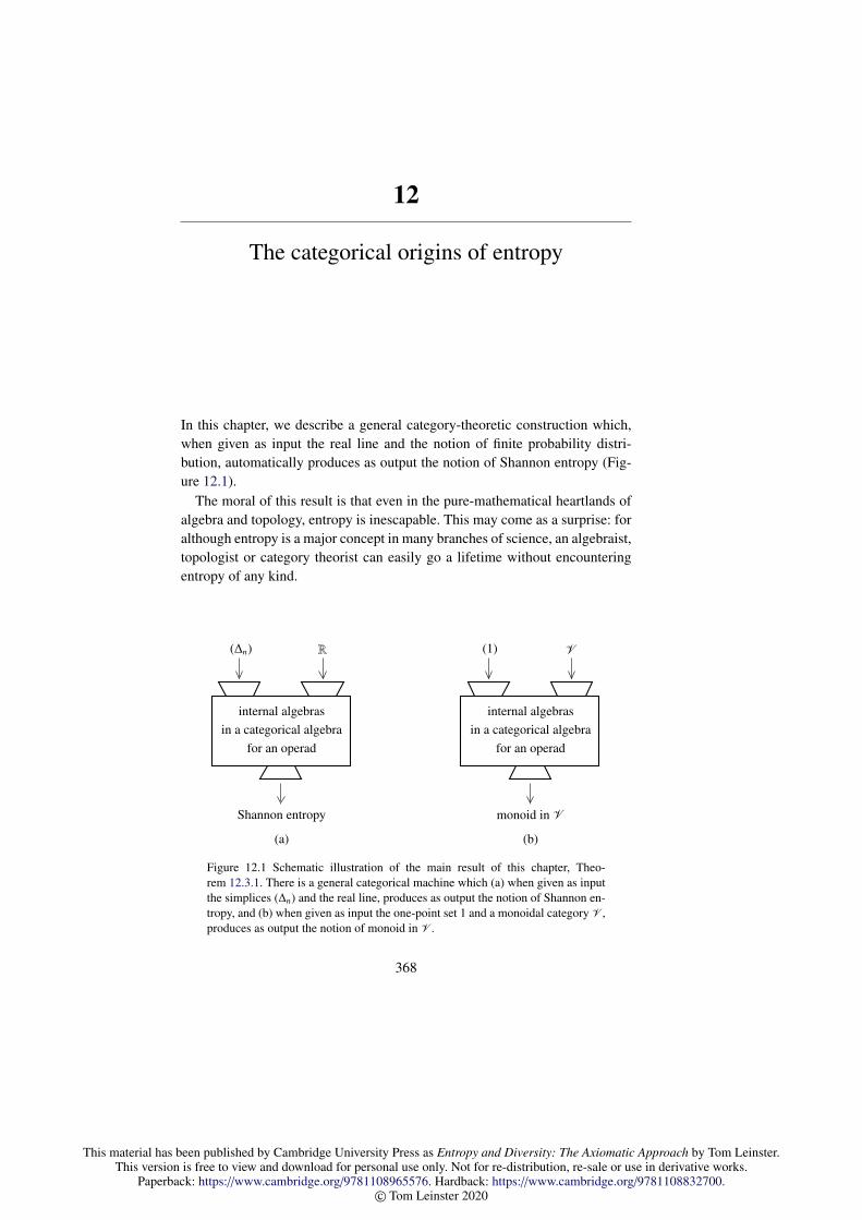
This material has been published by Cambridge University Press as Entropy and Diversity: The Axiomatic Approach by Tom Leinster.This version is free to view and download for personal use only. Not for re-distribution, re-sale or use in derivative works.
Paperback: https://www.cambridge.org/9781108965576. Hardback: https://www.cambridge.org/9781108832700.© Tom Leinster 2020
12
The categorical origins of entropy
In this chapter, we describe a general category-theoretic construction which,when given as input the real line and the notion of finite probability distri-bution, automatically produces as output the notion of Shannon entropy (Fig-ure 12.1).
The moral of this result is that even in the pure-mathematical heartlands ofalgebra and topology, entropy is inescapable. This may come as a surprise: foralthough entropy is a major concept in many branches of science, an algebraist,topologist or category theorist can easily go a lifetime without encounteringentropy of any kind.
internal algebrasin a categorical algebra
for an operad
(∆n) R
Shannon entropy
(a)
internal algebrasin a categorical algebra
for an operad
(1) V
monoid in V
(b)
Figure 12.1 Schematic illustration of the main result of this chapter, Theo-rem 12.3.1. There is a general categorical machine which (a) when given as inputthe simplices (∆n) and the real line, produces as output the notion of Shannon en-tropy, and (b) when given as input the one-point set 1 and a monoidal category V ,produces as output the notion of monoid in V .
368
This material has been published by Cambridge University Press as Entropy and Diversity: The Axiomatic Approach by Tom Leinster.This version is free to view and download for personal use only. Not for re-distribution, re-sale or use in derivative works.
Paperback: https://www.cambridge.org/9781108965576. Hardback: https://www.cambridge.org/9781108832700.© Tom Leinster 2020
12.1 Operads and their algebras 369
Yet the categorical construction described here is entirely general and natu-ral. It is not tailor-made for this particular purpose. Other familiar inputs pro-duce familiar outputs. And the inputs that we give to the construction here, thereal line R and the standard topological simplices ∆n, are fundamental objectsof pure mathematics. So, we are all but forced to accept Shannon entropy as anatural concept in pure mathematics too – quite independently of any motiva-tion in terms of information, diversity, thermodynamics, and so on.
The categorical construction involves operads and their algebras. The firsttwo sections set out some standard definitions, beginning with operads andalgebras themselves in Section 12.1. For an operad P, there are notions ofcategorical P-algebra A (a category acted on by P) and of internal algebra inA. With these definitions in place (Section 12.2), we can fulfil the promise ofthe first paragraph above (Theorem 12.3.1). Specifically, we show that for theoperad ∆ of simplices and the categorical ∆-algebra R, the internal algebras inR are precisely the scalar multiples of Shannon entropy.
In the final section, we describe the free categorical ∆-algebra containing aninternal algebra. The result proved is analogous to the classical theorem thatthe free monoidal category containing a monoid is the category of finite totallyordered sets. To reach this result involves a further climb up the mountain ofcategorical abstraction. But at the end of the path is a characterization of infor-mation loss that is entirely concrete. It is almost exactly the characterizationtheorem of Chapter 10.
This chapter assumes some knowledge of category theory, including theconcepts of product in a category, monoid in a monoidal category, and internalcategory in a category with finite limits.
12.1 Operads and their algebras
An operad is a system of abstract operations, somewhat like an algebraic the-ory in the sense of universal algebra, but more restricted in nature. Operads firstemerged in algebraic topology (Boardman and Vogt [44]; May [245]), whileindependently, the more general notion of multicategory was being developedin categorical logic (Lambek [199]). Nowadays, operads (like many other cat-egorical structures) have found application in a very wide range of subjects,from algebra to theoretical physics. Some samples of such applications can befound in Kontsevich [194], Loday and Vallette [232], and Markl, Shnider andStasheff [242].
Many introductions to operads are available, such as [232], [242], and Chap-

This material has been published by Cambridge University Press as Entropy and Diversity: The Axiomatic Approach by Tom Leinster.This version is free to view and download for personal use only. Not for re-distribution, re-sale or use in derivative works.
Paperback: https://www.cambridge.org/9781108965576. Hardback: https://www.cambridge.org/9781108832700.© Tom Leinster 2020
370 The categorical origins of entropy
θ
Figure 12.2 An element θ ∈ P4 of an operad P.
7→
θ
φ1 φ2 φ3
θ (φ1, φ2, φ3)
Figure 12.3 Composition in an operad: θ ∈ P3 composes with φ1 ∈ P2, φ2 ∈ P3
and φ3 ∈ P0 to give θ (φ1, φ2, φ3) ∈ P5.
ter 2 of [205]. Here we give only the definitions and results that are needed inorder to reach our goal.
An operad consists of a sequence (Pn)n≥0 of sets equipped with certain alge-braic structure obeying certain laws. It is useful to view the elements θ of Pn asabstract operations with n inputs and one output, as in Figure 12.2. A typicalexample will be given by Pn = A (A⊗n, A), for any object A of a monoidalcategory A . The algebraic structure on the sequence of sets (Pn)n≥0, and theequational laws that this structure obeys, are exactly those suggested by thisexample.
Definition 12.1.1 An operad P consists of:
• a sequence (Pn)n≥0 of sets;• for each n, k1, . . . , kn ≥ 0, a function
Pn × Pk1 × · · · × Pkn → Pk1+···+kn (12.1)
(Figure 12.3), called composition and written as
(θ, φ1, . . . , φn) 7→ θ (φ1, . . . , φn);
• an element 1P ∈ P1, called the identity,
satisfying the following axioms:

This material has been published by Cambridge University Press as Entropy and Diversity: The Axiomatic Approach by Tom Leinster.This version is free to view and download for personal use only. Not for re-distribution, re-sale or use in derivative works.
Paperback: https://www.cambridge.org/9781108965576. Hardback: https://www.cambridge.org/9781108832700.© Tom Leinster 2020
12.1 Operads and their algebras 371
θ
φ ψ
χ ξ ω
Figure 12.4 Every tree of operations in an operad P has a well-defined composite(in this case, an element of P9).
• associativity: for each n, ki, `i j ≥ 0 and θ ∈ Pn, φi ∈ Pki , ψi j ∈ P`i j ,(
θ (φ1, . . . , φn)) (
ψ11, . . . , ψ1k1 , . . . , ψn1, . . . , ψnkn)
= θ (φ1
(ψ11, . . . , ψ1k1
), . . . , φn
(ψn1, . . . , ψnkn
));
• identity: for each n ≥ 0 and θ ∈ Pn,
θ (1P, . . . , 1P︸ ︷︷ ︸n
) = θ = 1P (θ).
Every tree of operations such as that shown in Figure 12.4 has an unambigu-ous composite, obtained by repeatedly using the composition and identity ofthe operad. The associativity and identity axioms guarantee that the order inwhich this is done makes no difference to the outcome.
Examples 12.1.2 i. There is an operad 1 in which 1n is the one-element setfor each n ≥ 0. The composition and identities are uniquely determined.With the obvious notion of map of operads, 1 is the terminal operad.
ii. Fix a monoid M. There is an operad P(M) given by
P(M)n =
M if n = 1,
∅ otherwise
(n ≥ 0). There is no choice in how to define the composition of P(M) exceptwhen n = k1 = 1 (in the notation of (12.1)), and in that case it is defined tobe the multiplication of M. Similarly, the identity of the operad P(M) is theidentity of the monoid M.
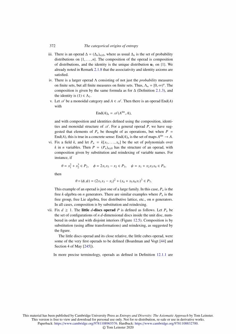
This material has been published by Cambridge University Press as Entropy and Diversity: The Axiomatic Approach by Tom Leinster.This version is free to view and download for personal use only. Not for re-distribution, re-sale or use in derivative works.
Paperback: https://www.cambridge.org/9781108965576. Hardback: https://www.cambridge.org/9781108832700.© Tom Leinster 2020
372 The categorical origins of entropy
iii. There is an operad ∆ = (∆n)n≥0, where as usual ∆n is the set of probabilitydistributions on 1, . . . , n. The composition of the operad is compositionof distributions, and the identity is the unique distribution u1 on 1. Wealready noted in Remark 2.1.8 that the associativity and identity axioms aresatisfied.
iv. There is a larger operad Λ consisting of not just the probability measureson finite sets, but all finite measures on finite sets. Thus, Λn = [0,∞)n. Thecomposition is given by the same formula as for ∆ (Definition 2.1.3), andthe identity is (1) ∈ Λ1.
v. Let A be a monoidal category and A ∈ A . Then there is an operad End(A)with
End(A)n = A (A⊗n, A),
and with composition and identities defined using the composition, identi-ties and monoidal structure of A . For a general operad P, we have sug-gested that elements of Pn be thought of as operations, but when P =
End(A), this is true in a concrete sense: End(A)n is the set of maps A⊗n → A.vi. Fix a field k, and let Pn = k[x1, . . . , xn] be the set of polynomials over
k in n variables. Then P = (Pn)n≥0 has the structure of an operad, withcomposition given by substitution and reindexing of variable names. Forinstance, if
θ = x21 + x3
2 ∈ P2, φ = 2x1x3 − x2 ∈ P3, ψ = x1 + x2x3x4 ∈ P4,
then
θ (φ, ψ) = (2x1x3 − x2)2 + (x4 + x5x6x7)3 ∈ P7.
This example of an operad is just one of a large family. In this case, Pn is thefree k-algebra on n generators. There are similar examples where Pn is thefree group, free Lie algebra, free distributive lattice, etc., on n generators.In all cases, composition is by substitution and reindexing.
vii. Fix d ≥ 1. The little d-discs operad P is defined as follows. Let Pn bethe set of configurations of n d-dimensional discs inside the unit disc, num-bered in order and with disjoint interiors (Figure 12.5). Composition is bysubstitution (using affine transformations) and reindexing, as suggested bythe figure.
The little discs operad and its close relative, the little cubes operad, weresome of the very first operads to be defined (Boardman and Vogt [44] andSection 4 of May [245]).
In more precise terminology, operads as defined in Definition 12.1.1 are

This material has been published by Cambridge University Press as Entropy and Diversity: The Axiomatic Approach by Tom Leinster.This version is free to view and download for personal use only. Not for re-distribution, re-sale or use in derivative works.
Paperback: https://www.cambridge.org/9781108965576. Hardback: https://www.cambridge.org/9781108832700.© Tom Leinster 2020
12.1 Operads and their algebras 373
1
2
3
1
2
21
34
θ
φ ψ
(a)
1
2
3
4 5
67
θ (φ, ψ)
(b)
Figure 12.5 (a) Operations θ ∈ P2, φ ∈ P3 and ψ ∈ P4 in the little 2-discs operadP (Example 12.1.2(vii)); (b) the composite operation θ (φ, ψ) ∈ P7.
called nonsymmetric operads of sets. Just as the definition of monoidal cate-gory has symmetric and nonsymmetric variants, so too does the definition ofoperad. We will concentrate on the nonsymmetric variant.
However, we will not only need operads of sets. Let E be any categorywith finite products (or indeed, any symmetric monoidal category, a level ofgenerality that we will not need). An operad in E is a sequence (Pn)n≥0 ofobjects of E together with maps (12.1) in E (encoding the composition) and amap 1→ P1 in E (encoding the identity), all subject to commutative diagramsexpressing the associativity and identity equations of Definition 12.1.1.
Details of this more general definition can be found in May [246], for in-stance, but we will need only two cases. The first is E = Set, the category ofsets. In that case, an operad in E is just an operad as in Definition 12.1.1. Thesecond is E = Top, the category of topological spaces. An operad in Top isjust an operad P of sets in which each set Pn is equipped with a topology andthe composition maps (12.1) are continuous. We will refer to operads in Topas topological operads.
Examples 12.1.3 i. The terminal operad 1 is a topological operad in a uniqueway.
ii. For a topological monoid M, the operad P(M) of Example 12.1.2(ii) is atopological operad in an evident way.
iii. Putting the standard topology on the simplices ∆n gives ∆ the structure of atopological operad.
iv. The little discs operad is also naturally a topological operad.

This material has been published by Cambridge University Press as Entropy and Diversity: The Axiomatic Approach by Tom Leinster.This version is free to view and download for personal use only. Not for re-distribution, re-sale or use in derivative works.
Paperback: https://www.cambridge.org/9781108965576. Hardback: https://www.cambridge.org/9781108832700.© Tom Leinster 2020
374 The categorical origins of entropy
An operad P is a system of abstract operations. An algebra for P is an inter-pretation of the elements of P as actual operations:
Definition 12.1.4 Let P be an operad of sets. A P-algebra is a set A togetherwith a map
αn : Pn × An → A(θ, (a1, . . . , an)
)7→ θ(a1, . . . , an)
for each n ≥ 0, satisfying two axioms:
θ (φ1, . . . , φn)(a11, . . . , a1k1 , . . . , an1, . . . , ankn
)= θ
(φ1(a11, . . . , a1k1
), . . . , φn(an1, . . . , ankn
))(12.2)
for all θ ∈ Pn, φi ∈ Pki and ai j ∈ A; and
1P(a) = a (12.3)
for all a ∈ A.
The definition of algebra extends easily from operads of sets to operadsin any category E with finite products: then A is an object of E and αn is amap in E , while the equations (12.2) and (12.3) are expressed as commutativediagrams in E (May [246]). In the only other case that concerns us here, E =
Top, an algebra for a topological operad P is a topological space A togetherwith a sequence of continuous maps(
Pn × An αn−→ A
)n≥0
satisfying equations (12.2) and (12.3).
Examples 12.1.5 i. Consider the terminal operad 1 of sets. A 1-algebra is aset A together with a map αn : An → A for each n ≥ 0, satisfying equa-tions (12.2) and (12.3). One easily deduces that a 1-algebra is exactly amonoid, with αn as its n-fold multiplication. If 1 is regarded as a topologi-cal operad then a 1-algebra is exactly a topological monoid.
ii. Fix a monoid M. An algebra for the operad P(M) is simply a set with a leftM-action. If M is a topological monoid then a P(M)-algebra is a topologicalspace with a continuous left M-action.
iii. Now consider the topological operad ∆ of simplices. Any convex subset Aof Rd, for any d ≥ 0, is a ∆-algebra in a natural way: given p ∈ ∆n anda1, . . . , an ∈ A, put
p(a1, . . . , an) = p1a1 + · · · + pnan ∈ A.

This material has been published by Cambridge University Press as Entropy and Diversity: The Axiomatic Approach by Tom Leinster.This version is free to view and download for personal use only. Not for re-distribution, re-sale or use in derivative works.
Paperback: https://www.cambridge.org/9781108965576. Hardback: https://www.cambridge.org/9781108832700.© Tom Leinster 2020
12.1 Operads and their algebras 375
Equations (12.2) and (12.3) express elementary facts about convex combi-nations.
We refer to this as the standard ∆-algebra structure on A.iv. The previous example admits a family of deformations, at least when A is
a linear subspace of Rd. For each q ∈ R, there is a ∆-algebra structure on Agiven by
p(a1, . . . , an) =∑
i∈supp ppq
i ai.
(Here the superscript q is a power but the superscript i is an index.) Theprevious example is the case q = 1.
v. The chain rule for a weighted mean M on an interval I nearly states that themaps (
M : ∆n × In → I)n≥0
give I the structure of an algebra for the operad ∆. More exactly, the chainrule is the composition axiom (12.2) for a ∆-algebra. For I to be a ∆-algebra,it must also satisfy the identity axiom (12.3), which is a special case ofconsistency: M(u1, (x)) = x for each x ∈ I.
vi. For any operad P of sets, a P-algebra amounts to a set A together with amap P→ End(A) of operads. Here, End(A) is the operad defined in Exam-ple 12.1.2(v), with A = Set. This makes precise the earlier assertion that analgebra for P is an interpretation of the elements of P as actual operations.
vii. Any d-fold loop space is an algebra for the little d-discs operad in a naturalway. This was one of the first examples of an algebra for an operad, thedetails of which can be found in Section 5 of May [245].
Let P be an operad in a finite product category E , and let A = (A, α) andB = (B, β) be P-algebras. A map of P-algebras from A to B is a map f : A→ Bin E such that the square
Pn × An 1× f n//
αn
Pn × Bn
βn
A
f// B
commutes for each n ≥ 0. This defines a category Alg(P) of P-algebras.
Remarks 12.1.6 The language of operations and algebras invites comparisonwith other categorical formulations of the concept of algebraic theory. System-atic comparisons can be found in Kelly [183], Section 2.8 of Gould [122], andChapter 3 of Avery [21]. Here, we just make the following observations.

This material has been published by Cambridge University Press as Entropy and Diversity: The Axiomatic Approach by Tom Leinster.This version is free to view and download for personal use only. Not for re-distribution, re-sale or use in derivative works.
Paperback: https://www.cambridge.org/9781108965576. Hardback: https://www.cambridge.org/9781108832700.© Tom Leinster 2020
376 The categorical origins of entropy
i. Let E be a finite product category satisfying the further mild condition thatit has countable coproducts over which the product distributes. (Set andTop are examples.) Then any operad P in E induces a monad TP on E ,with functor part given by
TP(A) =∐n≥0
Pn × An
(A ∈ E ). The category of algebras for the operad P is exactly the categoryof algebras for the monad TP. Non-isomorphic operads P sometimes inducethe same monad TP [206], although many aspects of an operad can still beunderstood through its induced monad.
ii. Remark (i) provides a semantic connection between operads and a differentconception of algebraic theory, monads. On the syntactic side, the definitionof operad can easily be adapted to give a definition of finitary algebraictheory, equivalent to any of the usual definitions (as given in Manes [240],for instance). Indeed, a finitary algebraic theory can be defined as an operadP together with, for each map of sets
f : 1, . . . ,m → 1, . . . , n,
a map f∗ : Pm → Pn, subject to equations expressing compatibility betweenthe operad structure and these maps f∗ (Tronin [326, 327]). The idea is thatf∗ transforms an m-ary operation into an n-ary operation by reindexing thevariables according to f . For instance, in the theory P of groups, Pn is theunderlying set of the free group on n generators (which can be regarded asthe set of n-ary operations defined on any group), and if f is the unique map1, 2 → 1 then f∗ : P2 → P1 sends the operation of multiplication to theoperation of squaring.
If we take the definition of finitary algebraic theory sketched in the pre-vious paragraph but restrict f to be a bijection, we obtain the definition ofsymmetric operad. (In much of the literature, ‘operad’ is taken to mean‘symmetric operad’ by default.) If we further restrict f to be an identity, werecover the definition of nonsymmetric operad.
iii. As the previous remark suggests, most algebraic theories cannot be de-scribed by an operad. For instance, there is no operad P of sets such thatAlg(P) is equivalent to the category of groups. For a proof of a strong ver-sion of this statement, see Lin [226].

This material has been published by Cambridge University Press as Entropy and Diversity: The Axiomatic Approach by Tom Leinster.This version is free to view and download for personal use only. Not for re-distribution, re-sale or use in derivative works.
Paperback: https://www.cambridge.org/9781108965576. Hardback: https://www.cambridge.org/9781108832700.© Tom Leinster 2020
12.2 Categorical algebras and internal algebras 377
12.2 Categorical algebras and internal algebras
Let P be an operad of sets. An algebra for P is a set acted on by P, but moregenerally, we can consider categories acted on by P. Such a structure is calleda categorical P-algebra.
More generally still, let E be a category with finite limits. Then there is thenotion of internal category in E (as in Chapter 2 of Johnstone [161]), and whenP is an operad in E , we can consider actions of P on such an internal category.
Definition 12.2.1 Let E be a category with finite limits and let P be an operadin E . A categorical P-algebra is an internal category in Alg(P).
It is straightforward to verify that Alg(P) has finite limits, computed as inE , so this definition does make sense. But it is also helpful to have at hand amore explicit form, as follows.
A categorical P-algebra A can be described as a pair of ordinary P-algebras,A0 and A1, together with domain and codomain maps
A1 ⇒ A0
and composition and identity maps
A1 ×A0 A1 → A1, 1→ A1,
all of which are required to be maps of P-algebras, as well as obeying the usualaxioms for an internal category. Here A0 is to be thought of as the object ofobjects of A, and A1 as the object of maps in A.
Equivalently, a categorical P-algebra is an internal category in E on whichP acts functorially. To see this, first note that for any object X of E and internalcategory A in E , we can define another internal category
X × A
in E . This is the product D(X)×A, where D(X) is the discrete internal categoryon X. Thus, its object of objects and object of maps are given by
(X × A)0 = X × A0, (X × A)1 = X × A1.
In this notation, a categorical P-algebra consists of an internal category A in E
together with internal functors
αn : Pn × An → A (12.4)
(n ≥ 0), satisfying analogues of the usual algebra axioms.As usual, we are principally concerned with the cases E = Set and E = Top,
where categorical algebras for an operad can be understood as follows.

This material has been published by Cambridge University Press as Entropy and Diversity: The Axiomatic Approach by Tom Leinster.This version is free to view and download for personal use only. Not for re-distribution, re-sale or use in derivative works.
Paperback: https://www.cambridge.org/9781108965576. Hardback: https://www.cambridge.org/9781108832700.© Tom Leinster 2020
378 The categorical origins of entropy
Examples 12.2.2 i. Let P be an operad in E = Set. A categorical P-algebraconsists of a small category A together with a functor
θ : An → A
for each n ≥ 0 and θ ∈ Pn. These functors are required to satisfy equa-tions (12.2) and (12.3) for objects ai j and a of A, and analogous equationsfor maps in A.
ii. Let P be an operad in E = Top. The categorical P-algebras can be describedas in (i), but with the following additions. A is now a topological cate-gory, so that A0 and A1 carry topologies with the property that the domain,codomain, composition and identity operations are continuous. Moreover,the structure maps
Pn × An0 → A0, Pn × An
1 → A1
of the P-algebras A0 and A1 are required to be continuous.iii. Here we consider the special case of categorical algebras with only one
object, over both Set and Top.First, let P be an operad of sets. Let A be a monoid, viewed as a one-
object category A. To give A the structure of a categorical P-algebra is togive the set A the structure of an ordinary P-algebra in such a way that foreach n ≥ 0 and θ ∈ Pn, the structure map
θ : An → A
is a monoid homomorphism. In short, a one-object categorical P-algebra isa monoid on which P acts by homomorphisms.
Similarly, when P is a topological operad, a one-object categorical P-algebra is a topological monoid on which P acts by continuous homomor-phisms.
Some specific examples now follow.
Examples 12.2.3 i. Consider the terminal operad of sets, 1. By the descrip-tion preceding equation (12.4), a categorical 1-algebra is a category onwhich 1 acts functorially, that is, a category A together with a functorAn → A, subject to certain axioms. These axioms give A the structure ofa monoid in Cat. Thus, a categorical 1-algebra is exactly a strict monoidalcategory.
Alternatively, working directly from Definition 12.2.1, a categorical 1-algebra is an internal category in Mon, the category of monoids. Again,this is just a strict monoidal category.

This material has been published by Cambridge University Press as Entropy and Diversity: The Axiomatic Approach by Tom Leinster.This version is free to view and download for personal use only. Not for re-distribution, re-sale or use in derivative works.
Paperback: https://www.cambridge.org/9781108965576. Hardback: https://www.cambridge.org/9781108832700.© Tom Leinster 2020
12.2 Categorical algebras and internal algebras 379
ii. Let M be a monoid, and form the operad P(M) of sets (Example 12.1.2(ii)).A categorical P(M)-algebra is a category equipped with a left M-action.
iii. Consider the topological operad ∆ of simplices. Let A be a linear subspace(or more generally, a convex additive submonoid) of Rd. Then A is a topo-logical monoid under addition. We have already considered the standard∆-algebra structure on the topological space A, given for p ∈ ∆n by
p : An → A(a1, . . . , an) 7→
∑ni=1 piai
(Example 12.1.5(iii)). Each of these maps p is a monoid homomorphism.Hence by Example 12.2.2(iii), A is a one-object categorical ∆-algebra.
iv. The same is true for the q-deformed algebra structure
(a1, . . . , an) 7→∑
i∈supp(p)
pqi ai
of Example 12.1.5(iv), for any q ∈ R.
For ordinary algebras for an operad, there is only one sensible notion of mapbetween algebras, but for categorical algebras, there are several. Indeed, let E
be a category with finite limits, let P be an operad in E , and let B and A becategorical P-algebras. Then B and A are, by definition, internal categories inAlg(P), and a strict map from B to A is an internal functor B→ A in Alg(P).Equivalently, it is an internal functor
G : B→ A
in E such that for all n ≥ 0, the square
Pn × Bn 1×Gn//
βn
Pn × An
αn
B
G// A
commutes, where βn and αn are the structure maps of B and A (as in equa-tion (12.4)).
However, this is a square of (internal) categories and functors, so we canalso consider variants in which the square is only required to commute up to aspecified natural isomorphism, or a natural transformation in one direction orthe other – subject, as usual, to coherence axioms. The particular variant thatwill concern us is the following.
Definition 12.2.4 Let E be a category with finite limits and let P be an operadin E . Let B and A be categorical P-algebras, with structure maps (βn) and (αn)
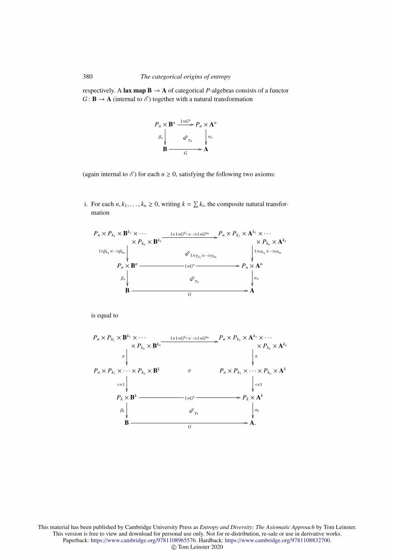
This material has been published by Cambridge University Press as Entropy and Diversity: The Axiomatic Approach by Tom Leinster.This version is free to view and download for personal use only. Not for re-distribution, re-sale or use in derivative works.
Paperback: https://www.cambridge.org/9781108965576. Hardback: https://www.cambridge.org/9781108832700.© Tom Leinster 2020
380 The categorical origins of entropy
respectively. A lax map B→ A of categorical P-algebras consists of a functorG : B→ A (internal to E ) together with a natural transformation
Pn × Bn 1×Gn//
βn
⇐γn
Pn × An
αn
B
G// A
(again internal to E ) for each n ≥ 0, satisfying the following two axioms:
i. For each n, k1, . . . , kn ≥ 0, writing k =∑
ki, the composite natural transfor-mation
Pn × Pk1 × Bk1 × · · ·
× Pkn × Bkn
⇐1×γk1×···×γkn
1×βk1×···×βkn
1×1×Gk1×···×1×Gkn //Pn × Pk1 × Ak1 × · · ·
× Pkn × Akn
1×αk1×···×αkn
Pn × Bn
⇐γnβn
1×Gn // Pn × An
αn
B
G// A
is equal to
Pn × Pk1 × Bk1 × · · ·
× Pkn × Bkn
1×1×Gk1×···×1×Gkn //Pn × Pk1 × Ak1 × · · ·
× Pkn × Akn
Pn × Pk1 × · · · × Pkn × Bk
×1
= Pn × Pk1 × · · · × Pkn × Ak
×1
Pk × Bk
⇐γkβk
1×Gk // Pk × Ak
αk
B
G// A.

This material has been published by Cambridge University Press as Entropy and Diversity: The Axiomatic Approach by Tom Leinster.This version is free to view and download for personal use only. Not for re-distribution, re-sale or use in derivative works.
Paperback: https://www.cambridge.org/9781108965576. Hardback: https://www.cambridge.org/9781108832700.© Tom Leinster 2020
12.2 Categorical algebras and internal algebras 381
ii. The composite natural transformation
B
G // A
1 × B
1P×1
= 1 × A
1P×1
P1 × B
⇐γ1β1
1×G // P1 × A
α1
B
G// A
is equal to the identity. (Here, 1P : 1 → P1 denotes the map encoding theidentity of the operad P.)
A strict map of P-algebras can equivalently be viewed as a lax map (G, γ) inwhich each of the maps γn is an identity.
Remark 12.2.5 Definition 12.2.4 can also be derived from the theory of 2-monads, as follows. We observed in Remark 12.1.6(i) that any operad P in E
induces a monad TP on E (under mild hypotheses on the category E ). In thesame way, it induces a 2-monad on Cat(E ), the 2-category of internal cate-gories in E . An algebra for that 2-monad is exactly a categorical P-algebra,and a lax map of algebras for the 2-monad (in the sense of Blackwell, Kellyand Power [41]) is exactly a lax map of categorical P-algebras.
As a general categorical principle, it is often worth considering the mapsinto an object from the terminal object. (In categories of spaces, this gives thenotion of point.) For any operad P in any category E with finite limits, there isa terminal categorical P-algebra 1. We consider the lax maps from 1 to othercategorical P-algebras.
Definition 12.2.6 Let E be a category with finite limits, let P be an operad inE , and let A be a categorical P-algebra. An internal algebra in A is a lax map1→ A of categorical P-algebras.
This definition is due to Batanin ([31], Definition 7.2). We will see that itgeneralizes the notion of internal monoid in a monoidal category. But first,we give an explicit description of internal algebras in the cases E = Set andE = Top.
Examples 12.2.7 i. Let E = Set. Take an operad P of sets and a categori-cal P-algebra A. An internal algebra in A consists of, first of all, a functor

This material has been published by Cambridge University Press as Entropy and Diversity: The Axiomatic Approach by Tom Leinster.This version is free to view and download for personal use only. Not for re-distribution, re-sale or use in derivative works.
Paperback: https://www.cambridge.org/9781108965576. Hardback: https://www.cambridge.org/9781108832700.© Tom Leinster 2020
382 The categorical origins of entropy
G : 1 → A. This simply picks out an object a of A. Next, the natural trans-formations γn in Definition 12.2.4 amount to a family of maps
γθ : θ(a, . . . , a︸ ︷︷ ︸n
)→ a,
one for each n ≥ 0 and θ ∈ Pn. The first coherence axiom in Defini-tion 12.2.4 states that the diagram
θ(φ1(a, . . . , a), . . . , φn(a, . . . , a)
) θ(γφ1 ,...,γφn )// θ(a, . . . , a)
γθ
θ (φ1, . . . , φn)(a, . . . , a)
γθ(φ1 ,...,φn )
// a
commutes for all θ ∈ Pn and φi ∈ Pki , and the second states that
γ1P : 1P(a)→ a
is equal to the identity on a.ii. An identical description of internal algebras applies when E = Top, with
the additional condition that for each n ≥ 0, the function
Pn → A1
θ 7→ γθ
is continuous. (Here A1 denotes the space of maps in the topological cate-gory A, as in Example 12.2.2(ii).)
iii. Now let E = Set, and let A be a one-object categorical P-algebra. As wesaw in Example 12.2.2(iii), A amounts to a monoid A on which P acts byhomomorphisms. An internal P-algebra in A consists of an element γθ ∈ Afor each n ≥ 0 and θ ∈ Pn, satisfying the coherence axioms in (i).
Writing γθ as γ(θ), we have a sequence of functions(γ : Pn → A
)n≥0.
The coherence axioms in (i) state that
γ(θ) · θ(γ(φ1), . . . , γ(φn)
)= γ
(θ (φ1, . . . , φn)
)(12.5)
for all n, k1, . . . , kn ≥ 0, θ ∈ Pn and φi ∈ Pki , and that
γ(1P) = 1. (12.6)
In summary, when A is a one-object categorical P-algebra correspondingto a monoid A, an internal P-algebra in A amounts to a sequence of mapsγ : Pn → A satisfying equations (12.5) and (12.6).

This material has been published by Cambridge University Press as Entropy and Diversity: The Axiomatic Approach by Tom Leinster.This version is free to view and download for personal use only. Not for re-distribution, re-sale or use in derivative works.
Paperback: https://www.cambridge.org/9781108965576. Hardback: https://www.cambridge.org/9781108832700.© Tom Leinster 2020
12.2 Categorical algebras and internal algebras 383
iv. For a topological operad P, internal algebras in a one-object categorical P-algebra admit exactly the same explicit description as in the previous exam-ple, with the added requirement that the maps γ : Pn → A are continuous.
We now give some specific examples.
Examples 12.2.8 i. Let 1 be the terminal operad of sets. As we have seen, acategorical 1-algebra is just a monoidal category. By the explicit descrip-tion in Example 12.2.7(i), an internal algebra in a categorical 1-algebra Aconsists of an object a ∈ A together with a map
γn : a⊗n → a
for each n ≥ 0, satisfying the equations given there. It follows easily that aninternal algebra in A is exactly a monoid in the monoidal category A.
As an alternative proof, note that for strict monoidal categories B andA, a lax map B → A of categorical 1-algebras is precisely a lax monoidalfunctor. This is immediate from the definitions. Hence an internal algebrain a strict monoidal category A is a lax monoidal functor 1 → A, andit is well-known that such functors correspond naturally to monoids in A(paragraph (5.4.1) of Benabou [34]).
An algebra for 1 is exactly a monoid (Example 12.1.5(i)), so it is logicalterminology that an internal algebra is exactly an internal monoid.
ii. Fix a monoid M. We saw in Example 12.2.3(ii) that a categorical P(M)-algebra is a category A with a left M-action; let us write the action as
M × A → A(m, a) 7→ m · a.
By the explicit description in Example 12.2.7(i), an internal P(M)-algebrain A consists of an object a ∈ A together with a map
γm : m · a→ a
for each m ∈ M, satisfying natural coherence axioms.
Missing from this list of examples is the case of internal algebras in a cat-egorical algebra for ∆, the operad of simplices. This is the subject of the nextsection, and will transport us directly to the concept of entropy.

This material has been published by Cambridge University Press as Entropy and Diversity: The Axiomatic Approach by Tom Leinster.This version is free to view and download for personal use only. Not for re-distribution, re-sale or use in derivative works.
Paperback: https://www.cambridge.org/9781108965576. Hardback: https://www.cambridge.org/9781108832700.© Tom Leinster 2020
384 The categorical origins of entropy
12.3 Entropy as an internal algebra
In this chapter so far, we have reviewed some established general conceptsin the theory of operads. We now apply them to the topological operad ∆ ofsimplices.
We saw in Example 12.2.3(iii) that the real line R, as a topological monoidunder addition, is a categorical ∆-algebra in a standard way:
(p, (x1, . . . , xn)
)7→
n∑i=1
pixi (12.7)
(p ∈ ∆n, x1, . . . , xn ∈ R). What are the internal algebras in the categorical∆-algebra R?
By Example 12.2.7(iv), an internal ∆-algebra in R amounts to a sequence offunctions
(γ : ∆n → R
)n≥0 satisfying certain axioms. It is in this sense that the
following theorem holds.
Theorem 12.3.1 Let ∆ be the topological operad of simplices, and equip Rwith its standard categorical ∆-algebra structure (12.7). Then the internal al-gebras in R are precisely the real scalar multiples of Shannon entropy.
In other words, a sequence of functions(γ : ∆n → R
)n≥0 defines an internal
algebra in R if and only if γ = cH for some c ∈ R.
Proof By Example 12.2.7(iv), an internal algebra in R is a sequence of func-tions
(γ : ∆n → R
)n≥0 with the following properties:
i. for all n, k1, . . . , kn ≥ 0 and w ∈ ∆n, p1 ∈ ∆k1 , . . . ,pn ∈ ∆kn ,
γ(w) +
n∑i=1
wiγ(pi) = γ(w (p1, . . . ,pn)
);
ii. γ(u1) = 0;iii. γ : ∆n → R is continuous for each n ≥ 0.
Condition (ii) is redundant, since it follows from (i) by taking n = k1 = 1 andw = p1 = u1. Hence by Faddeev’s Theorem 2.5.1, γ defines an internal algebraif and only if γ = cH for some c ∈ R.
This theorem can be deformed. In Example 12.2.3(iv), we defined a one-parameter family of categorical ∆-algebra structures on R, where for a realparameter q, the action of ∆ on R is(
p, (x1, . . . , xn))7→
∑i∈supp(p)
pqi xi (12.8)
(p ∈ ∆n, x1, . . . , xn ∈ R).

This material has been published by Cambridge University Press as Entropy and Diversity: The Axiomatic Approach by Tom Leinster.This version is free to view and download for personal use only. Not for re-distribution, re-sale or use in derivative works.
Paperback: https://www.cambridge.org/9781108965576. Hardback: https://www.cambridge.org/9781108832700.© Tom Leinster 2020
12.4 The universal internal algebra 385
Theorem 12.3.2 Let 1 , q ∈ R. Let ∆ be the operad of simplices, consideredas an operad of sets, and equip R with its q-deformed categorical ∆-algebrastructure (12.8). Then the internal algebras in R are precisely the real scalarmultiples of q-logarithmic entropy.
Proof By Example 12.2.7(iii), an internal algebra in R is a sequence of func-tions
(γ : ∆n → R
)n≥0 with the following properties:
i. for all n, k1, . . . , kn ≥ 0 and all w ∈ ∆n, p1 ∈ ∆k1 , . . . ,pn ∈ ∆kn ,
γ(w) +∑
i∈supp(w)
wqi γ(pi) = γ
(w (p1, . . . ,pn)
);
ii. γ(u1) = 0.
Condition (ii) is redundant, for the same reason as in the proof of Theo-rem 12.3.1. Condition (i) is satisfied if γ = cS q, by the chain rule (4.2) forq-logarithmic entropies. Conversely, condition (i) implies that
γ(w ⊗ p) = γ(w) +
( ∑i∈supp(w)
wqi
)γ(p)
for all w ∈ ∆n and p ∈ ∆k, by taking p1 = · · · = pn = p. Hence by Theo-rem 4.1.5, if γ defines an internal algebra then γ = cS q for some c ∈ R.
Continuity was not needed in this theorem, and in fact the structure maps∆n × R
n → R of the q-deformed ∆-algebra R are discontinuous when q ≤ 0.But they are evidently continuous when q > 0, so we have:
Corollary 12.3.3 Let q ∈ (0,∞). Let ∆ be the topological operad of sim-plices, and equip R with its q-deformed categorical ∆-algebra structure (12.8).Then the internal algebras in R are precisely the real scalar multiples of q-logarithmic entropy.
Proof The case q = 1 is Theorem 12.3.1, and all other cases follow fromTheorem 12.3.2.
12.4 The universal internal algebra
In algebra, an important role is played by free algebraic structures (groups,modules, etc.). But since one forms the free algebraic structure on a set, anda set is merely a cardinality (for these purposes at least), the possibilities arein a sense limited. Greater riches are to be found one categorical level up,where one can speak of the free categorical structure containing some specified
This material has been published by Cambridge University Press as Entropy and Diversity: The Axiomatic Approach by Tom Leinster.This version is free to view and download for personal use only. Not for re-distribution, re-sale or use in derivative works.
Paperback: https://www.cambridge.org/9781108965576. Hardback: https://www.cambridge.org/9781108832700.© Tom Leinster 2020
386 The categorical origins of entropy
internal algebraic structure. This leads to categorical characterizations of someimportant mathematical objects.
Examples 12.4.1 i. The free monoidal category containing a monoid isequivalent to the category of finite totally ordered sets (Mac Lane [234],Proposition VII.5.1). We will return to this example shortly. Informally, thestatement is that if we build a monoidal category by starting from noth-ing, putting in an internal monoid, then adjoining no more other objectsand maps than are forced by the definitions, and making no unnecessaryidentifications, then the result is the category of finite totally ordered sets.
ii. The free monoidal category containing an object A and an isomorphismA ⊗ A → A is equivalent to the disjoint union of the terminal categoryand Thompson’s group F, viewed as a one-object category (Fiore and Le-inster [102]).
(Thompson’s group is an infinite group with remarkable properties; it hasbeen rediscovered multiple times in diverse contexts. Cannon, Floyd andParry [58] provide a survey. A major open question, which has attractedan exceptional number of opposing claims and retractions, is whether F isamenable. Cannon and Floyd [57] report that even among experts, opinionis evenly split.)
iii. The free symmetric monoidal category containing a commutative Frobeniusalgebra is the category of compact oriented 1-manifolds and 2-dimensionalcobordisms between them (Theorem 3.6.19 of Kock [189], for instance).This result lies at the foundations of topological quantum field theory.
iv. The free finite product category containing a group is the Lawvere theory ofgroups. The same statement holds for any other algebraic structure in placeof groups (Lawvere [201]). This is essentially a tautology, but expressesa fundamental insight of categorical universal algebra: an algebraic theorycan be understood as a finite product category, and a model of a theory as afinite-product-preserving functor.
In this section, we construct the free categorical P-algebra containing aninternal algebra, where P is any given operad. We proceed as follows. First,we construct a certain categorical P-algebra FP. Then, we make precise whatit means for a categorical P-algebra to be ‘free containing an internal algebra’.Next, we prove that FP has that property. This last result, applied in the caseP = ∆, leads to a characterization of information loss.
We begin by constructing the categorical P-algebra FP, for an operad P ofsets.
The objects of FP are the pairs (n, θ) with n ≥ 0 and θ ∈ Pn. Where con-fusion will not arise, we write (n, θ) as just θ. For objects ψ = (k, ψ) and
This material has been published by Cambridge University Press as Entropy and Diversity: The Axiomatic Approach by Tom Leinster.This version is free to view and download for personal use only. Not for re-distribution, re-sale or use in derivative works.
Paperback: https://www.cambridge.org/9781108965576. Hardback: https://www.cambridge.org/9781108832700.© Tom Leinster 2020
12.4 The universal internal algebra 387
θ = (n, θ), a map ψ → θ in FP consists of integers k1, . . . , kn ≥ 0 and op-erations φ1 ∈ Pk1 , . . . , φ
n ∈ Pkn such that
k = k1 + · · · + kn, ψ = θ (φ1, . . . , φn).
We write this map as
〈φ1, . . . , φn〉θ : ψ→ θ. (12.9)
Thus, the set of objects of the category FP and the set of maps in FP are,respectively, ∐
n≥0
Pn,∐
n,k1,...,kn≥0
Pn × Pk1 × · · · × Pkn . (12.10)
Composition and identities in the category FP are defined using the composi-tion and identity of the operad P.
To give the category FP the structure of a categorical P-algebra, we mustconstruct from each operation π ∈ Pm a functor
π : (FP)m → FP.
On objects, π is defined by
π(θ1, . . . , θm) = π (θ1, . . . , θm).
To define the action of π on maps, take an m-tuple of maps
〈φ11, . . . , φ1n1〉θ1 : ψ1 → θ1
...
〈φm1, . . . , φmnm〉θm : ψm → θm
in FP. Then
π(〈φ11, . . . , φ1n1〉θ1 , . . . , 〈φm1, . . . , φmnm〉θm
)= 〈φ11, . . . , φ1n1 , . . . , φm1, . . . , φmnm〉π(θ1,...,θm), (12.11)
which is a map π(ψ1, . . . , ψm)→ π(θ1, . . . , θm) in FP.Verifying that FP satisfies the axioms for a categorical P-algebra is routine.
Lemma 12.4.2 Let P be an operad of sets.
i. The object 1P of FP is terminal.ii. Write !φ : φ → 1P for the unique map from an object φ of FP to 1P. Then
for any map
〈φ1, . . . , φn〉θ : ψ→ θ
This material has been published by Cambridge University Press as Entropy and Diversity: The Axiomatic Approach by Tom Leinster.This version is free to view and download for personal use only. Not for re-distribution, re-sale or use in derivative works.
Paperback: https://www.cambridge.org/9781108965576. Hardback: https://www.cambridge.org/9781108832700.© Tom Leinster 2020
388 The categorical origins of entropy
in FP, we have
〈φ1, . . . , φn〉θ = θ(!φ1 , . . . , !φn ).
The notation in (i) refers to the identity element 1P ∈ P1 of the operad P,which corresponds to the object 1P = (1, 1P) of the category FP. It is thisobject that is terminal.
Proof For (i), given any object φ of FP, it is immediate from the definition ofFP that there is a unique map φ→ 1P, namely,
!φ = 〈φ〉1P : φ→ 1P.
For (ii), take a map
〈φ1, . . . , φn〉θ : ψ→ θ
in FP. Since !φi is a map φi → 1P, the map θ(!φ1 , . . . , !φn ) has domain
θ(φ1, . . . , φn) = θ (φ1, . . . , φn) = ψ
and codomain
θ(1P, . . . , 1P) = θ (1P, . . . , 1P) = θ,
matching the domain and codomain of 〈φ1, . . . , φn〉θ. Now by definition of !φi
and by definition (12.11) of the P-action on maps in FP,
θ(!φ1 , . . . , !φn ) = θ(〈φ1〉1P , . . . , 〈φ
n〉1P
)= 〈φ1, . . . , φn〉θ(1P,...,1P)
= 〈φ1, . . . , φn〉θ,
as required.
The categorical P-algebra FP contains a canonical internal algebra. To spec-ify it, we use the description of internal algebras in Example 12.2.7(i). Its un-derlying object is the terminal object 1P. To give 1P the structure of an internalalgebra, we have to specify, for each n ≥ 0 and θ ∈ Pn, a map
θ(
1P, . . . , 1P︸ ︷︷ ︸n
)→ 1P.
The domain here is θ, and the codomain is terminal, so the only possible choiceis the unique map !θ : θ → 1P. This gives 1P the structure of an internal algebrain the categorical P-algebra FP. We refer to this internal algebra as (1P, !).
When P is a topological operad, the set of objects of FP and the set of mapsin FP (both given in (12.10)) each carry a natural topology. For instance, the setof maps in FP is a coproduct of product spaces. In this way, FP is an internal

This material has been published by Cambridge University Press as Entropy and Diversity: The Axiomatic Approach by Tom Leinster.This version is free to view and download for personal use only. Not for re-distribution, re-sale or use in derivative works.
Paperback: https://www.cambridge.org/9781108965576. Hardback: https://www.cambridge.org/9781108832700.© Tom Leinster 2020
12.4 The universal internal algebra 389
category in Top. Indeed, FP is a categorical P-algebra in the topological sense(by the description in Example 12.2.2(ii)) and (1P, !) is an internal algebra inFP in the topological sense (by the description in Example 12.2.7(iv).)
Remark 12.4.3 As for all of the operadic definitions and constructions in thischapter, the construction of FP can be generalized to an operad P in an ar-bitrary category E with suitable properties (in this case, finite products andcountable coproducts over which the products distribute). The general defini-tion is exactly as suggested by the case E = Top.
Examples 12.4.4 i. Consider the terminal operad 1 of sets. The objects ofthe category D = F1 are the natural numbers 0, 1, . . . A map k → n in Dis an ordered n-tuple of natural numbers summing to k, or equivalently, anorder-preserving map 1, . . . , k → 1, . . . , n. Thus, D is equivalent to thecategory of finite totally ordered sets. It is almost the same as the categoryusually denoted by ∆ in algebraic topology, the only difference being that italso contains the object 0 (corresponding to the empty ordered set).
By construction, D is a categorical 1-algebra, that is, a strict monoidalcategory. The monoidal structure is defined on objects by addition and onmaps by disjoint union. Moreover, D contains a canonical internal algebra,that is, internal monoid. It is the object 1 ∈ D with its unique monoid struc-ture: the multiplication is the unique map 1 + 1 = 2 → 1 in D, and theidentity is the unique map 0→ 1.
ii. Fix a monoid M and consider the operad P(M). Since P(M)n is empty forall n , 1, the objects of the category FP(M) are just the elements θ ∈ M. Amap ψ→ θ in FP(M) is an element φ ∈ M such that ψ = θφ. In other words,regarding the monoid M as a category with a single object ?, the categoryFP(M) is the slice M/?. For instance, when the monoid M is cancellative,FP(M) is the poset of elements of M ordered by divisibility.
iii. Now take the topological operad ∆. The objects of the category F∆ are thepairs (n,p) with n ≥ 0 and p ∈ ∆n. A map (k, s)→ (n,p) consists of naturalnumbers k1, . . . , kn summing to k together with probability distributions ri ∈
∆ki satisfying
s = p (r1, . . . , rn). (12.12)
This category has a more familiar description. As in (i) above, the n-tuple(k1, . . . , kn) amounts to an order-preserving map
f : 1, . . . , k → 1, . . . , n.
Then p is equal to the pushforward f s of the probability measure s along f .
This material has been published by Cambridge University Press as Entropy and Diversity: The Axiomatic Approach by Tom Leinster.This version is free to view and download for personal use only. Not for re-distribution, re-sale or use in derivative works.
Paperback: https://www.cambridge.org/9781108965576. Hardback: https://www.cambridge.org/9781108832700.© Tom Leinster 2020
390 The categorical origins of entropy
(See Definition 2.1.10.) Thus, f is a measure-preserving map(1, . . . , k, s
)→
(1, . . . , n,p
).
In Lemma 2.1.9, we showed that given s, p and k1, . . . , kn (or equivalentlys, p and f ), it is always possible to find distributions ri satisfying equa-tion (12.12). Furthermore, we showed that for i ∈ supp(p), the distributionri is uniquely determined, and for i < supp(p), we can choose ri freely in∆ki .
These observations together imply that up to equivalence, F∆ is the cat-egory whose objects are finite totally ordered probability spaces (X,p), inwhich a map (Y, s) → (X,p) is an order-preserving, measure-preservingmap f together with a probability distribution on f −1(i) for each i ∈ X suchthat pi = 0.
By construction, F∆ has the structure of a categorical ∆-algebra. On ob-jects, the ∆-action takes convex combinations of finite probability spaces,as in Section 10.1. The one-element probability space (1,u1) has a uniqueinternal algebra structure in F∆.
Remark 12.4.5 The category F∆ just described is nearly the categoryFinOrdProb of finite totally ordered probability spaces. There is a forget-ful functor F∆ → FinOrdProb, but it is not an equivalence, because of thecomplication associated with zero probabilities.
From the point of view of Bayesian inference, it is broadly unsurprisingthat such a complication arises. In that subject, special caution is reserved forprobabilities of exactly zero. The Bayesian statistician Dennis Lindley wrote:
leave a little probability for the moon being made of green cheese; it canbe as small as 1 in a million, but have it there since otherwise an armyof astronauts returning with samples of the said cheese will leave youunmoved. [. . . ] So never believe in anything absolutely, leave some roomfor doubt.
([228], p. 104.) He named this principle Cromwell’s rule, after the EnglishLord Protector Oliver Cromwell, who wrote to the Church of Scotland in 1650:
I beseech you, in the bowels of Christ, think it possible you may be mis-taken.
Further discussion can be found in Section 6.8 of Lindley [229].
We now make precise, and prove, the statement that FP is the ‘free categor-ical P-algebra containing an internal algebra’.
Let P be an operad of sets or topological spaces, and let E : B → A be

This material has been published by Cambridge University Press as Entropy and Diversity: The Axiomatic Approach by Tom Leinster.This version is free to view and download for personal use only. Not for re-distribution, re-sale or use in derivative works.
Paperback: https://www.cambridge.org/9781108965576. Hardback: https://www.cambridge.org/9781108832700.© Tom Leinster 2020
12.4 The universal internal algebra 391
a strict map of categorical P-algebras. An internal algebra in B is a lax map1 → B, and can be composed with E to obtain a lax map 1 → A. In this way,E maps internal algebras in B to internal algebras in A.
It will be convenient to use the explicit description of internal algebras de-rived in Example 12.2.7(i). There, we showed that an internal algebra (b, δ) inB consists of an object b and a family of maps δθ : θ(b, . . . , b) → b subjectto certain equations. In these terms, the induced internal algebra E(b, δ) in Aconsists of the object E(b) and the maps E(δθ).
We now state and prove the universal property of the categorical P-algebraFP equipped with its internal algebra (1P, !).
Theorem 12.4.6 Let P be an operad of either sets or topological spaces, letA be a categorical P-algebra, and let (a, γ) be an internal algebra in A. Thenthere is a unique strict map E : FP → A of categorical P-algebras such thatE(1P, !) = (a, γ).
This is a universal property of FP together with its internal algebra, andtherefore determines them uniquely up to isomorphism.
Proof To prove uniqueness, let E be a map with the properties stated. Letθ = (n, θ) be an object of FP; thus, n ≥ 0 and θ ∈ Pn. By definition of thecategorical P-algebra structure on FP,
θ = θ(1P, . . . , 1P).
Applying E to both sides gives
E(θ) = E(θ(1P, . . . , 1P)
)= θ
(E(1P), . . . , E(1P)
)= θ(a, . . . , a),
where the second equality holds because E is a strict map of categorical P-algebras, and the last is by hypothesis. Hence
E(θ) = θ(a, . . . , a), (12.13)
which determines E uniquely on the objects of FP.To show the same for maps, take a map
〈φ1, . . . , φn〉θ : ψ→ θ
in FP. By Lemma 12.4.2(ii),
〈φ1, . . . , φn〉θ = θ(!φ1 , . . . , !φn ).

This material has been published by Cambridge University Press as Entropy and Diversity: The Axiomatic Approach by Tom Leinster.This version is free to view and download for personal use only. Not for re-distribution, re-sale or use in derivative works.
Paperback: https://www.cambridge.org/9781108965576. Hardback: https://www.cambridge.org/9781108832700.© Tom Leinster 2020
392 The categorical origins of entropy
Applying E to both sides gives
E(〈φ1, . . . , φn〉θ
)= E
(θ(!φ1 , . . . , !φn )
)= θ
(E(!φ1 ), . . . , E(!φn )
)= θ(γφ1 , . . . , γφn ),
for the same reasons as in the argument for objects. Hence
E(〈φ1, . . . , φn〉θ
)= θ(γφ1 , . . . , γφn ), (12.14)
which determines E uniquely on the maps in FP. We have therefore proveduniqueness.
To prove existence, we define E on objects by equation (12.13) and on mapsby equation (12.14). Verifying that E satisfies the stated conditions (includingcontinuity in the topological case) is a series of routine checks.
Corollary 12.4.7 Let P be an operad of sets or topological spaces. Let A bea categorical P-algebra. Then there is a canonical bijection between internalalgebras in A and strict maps FP→ A of categorical P-algebras.
Thus, an internal algebra in A can be described as either a lax map 1 → Aor a strict map FP→ A.
Example 12.4.8 In the case P = 1, Theorem 12.4.6 states that for any strictmonoidal category A and monoid a in A, there is exactly one strict monoidalfunctor E : D → A that maps the trivial monoid 1 in D to the given monoid ain A.
Hence, Corollary 12.4.7 implies that given just a monoidal category A, themonoids in A correspond naturally to the strict monoidal functors D→ A. Wehave therefore recovered the classical fact that a monoid in A can be describedas either a lax monoidal functor 1 → A or a strict monoidal functor D → A(paragraph (5.4.1) of Benabou [34] and Proposition VII.5.1 of Mac Lane [234],for instance).
Now consider Theorem 12.4.6 in the case where P is the topological operad∆ and A is the topological monoid R. By Corollary 12.4.7, the strict mapsF∆ → A of categorical ∆-algebras are in natural bijection with the internal∆-algebras in A. By Theorem 12.3.1, these in turn correspond to real scalarmultiples of Shannon entropy. Together, these results imply that the strict mapsF∆→ A are naturally parametrized by R.
We now make this parametrization explicit. Since A has only one object, astrict map F∆→ A of categorical ∆-algebras amounts to a function
E : maps in F∆ → R

This material has been published by Cambridge University Press as Entropy and Diversity: The Axiomatic Approach by Tom Leinster.This version is free to view and download for personal use only. Not for re-distribution, re-sale or use in derivative works.
Paperback: https://www.cambridge.org/9781108965576. Hardback: https://www.cambridge.org/9781108832700.© Tom Leinster 2020
12.4 The universal internal algebra 393
satisfying certain conditions. Our final theorem classifies such functions.
Theorem 12.4.9 Let E be a function maps in F∆ → R. The following areequivalent:
i. E defines a strict map F∆ → R of categorical ∆-algebras in Top (withrespect to the standard categorical ∆-algebra structure on R);
ii. there is some c ∈ R such that for all maps f : s→ p in F∆,
E( f ) = c(H(s) − H(p)
).
Proof First assume (i). Applying E to the internal algebra (u1, !) in F∆ givesan internal algebra E(u1, !) in R (whose underlying object is necessarily theunique object of the category R). So by Theorem 12.3.1, there is some constantc ∈ R such that E(!p) = cH(p) for all n ≥ 1 and p ∈ ∆n.
Now take any map
〈r1, . . . , rn〉p : s→ p (12.15)
in F∆. Since u1 is terminal in F∆, there is a commutative triangle
s〈r1,...,rn〉p //
!s
p
!pu1
(12.16)
in F∆. Applying the functor E to this triangle gives
E(!s) = E(!p) + E(〈r1, . . . , rn〉p
), (12.17)
which by the result of the last paragraph gives
cH(s) = cH(p) + E(〈r1, . . . , rn〉p
),
proving (ii).To show that (ii) implies (i), let c ∈ R. By Theorem 12.3.1, cH defines an
internal algebra structure on the unique object of the category R. Now take amap (12.15) in F∆. By definition of E,
E(〈r1, . . . , rn〉p
)= c
(H(s) − H(p)
).
But s = p (r1, . . . , rn) by definition of the maps in F∆, so by the chain rule,
E(〈r1, . . . , rn〉p
)= c
n∑i=1
piH(ri) = p(cH(r1), . . . , cH(rn)
).
It follows from the proof of Theorem 12.4.6 that E is a strict map F∆ → R ofcategorical ∆-algebras.
This material has been published by Cambridge University Press as Entropy and Diversity: The Axiomatic Approach by Tom Leinster.This version is free to view and download for personal use only. Not for re-distribution, re-sale or use in derivative works.
Paperback: https://www.cambridge.org/9781108965576. Hardback: https://www.cambridge.org/9781108832700.© Tom Leinster 2020
394 The categorical origins of entropy
A result similar to Theorem 12.4.9 can also be proved for the q-logarithmicentropies, using the q-deformed categorical ∆-algebra structure on R and The-orem 12.3.2.
Theorem 12.4.9 bears a striking resemblance to the characterization of in-formation loss in Theorem 10.2.1. It states that the strict maps F∆ → R arethe scalar multiples of the information loss function. But where one theoremuses the category F∆, the other uses the category FinProb of finite probabil-ity spaces. The explicit description of F∆ in Example 12.4.4(iii) shows thatthere are three differences between F∆ and FinProb. First, the maps in F∆
are required to be order-preserving, whereas in FinProb there is no notion ofordering at all. Second, the category F∆ is skeletal (isomorphic objects areequal), but FinProb is not. Third, the maps in the category F∆ are not merelymeasure-preserving maps; they also come equipped with a probability distri-bution on the fibre over each zero-probability element of the codomain.
There is an analogue of Theorem 12.4.9 that comes close to Theorem 10.2.1;we sketch it now. It uses symmetric operads. As indicated in Remark 12.1.6(ii),a symmetric operad is an operad P together with an action of the symmetricgroup S n on Pn for each n ≥ 0, satisfying suitable axioms. For example, ifA is an object of a symmetric monoidal category then the operad End(A) ofExample 12.1.2(v) has the structure of a symmetric operad. The operad ∆ isalso symmetric in a natural way.
At the cost of some further complications, the notions of categorical P-algebra and internal algebra, and the construction of the free categorical P-algebra on an internal algebra, can be extended to symmetric operads P. Thefree categorical ∆-algebra Fsym∆ on an internal algebra is much like F∆, butthe maps are no longer required to be order-preserving. In other words, thefirst of the three differences between F∆ and FinProb vanishes for Fsym∆. Thesecond, skeletality, is categorically unimportant. So, the only substantial differ-ence between Fsym∆ and FinProb is the third: a map in Fsym∆ between finiteprobability spaces is a measure-preserving map together with a probability dis-tribution on each fibre over an element of probability zero.
The symmetric analogue of Theorem 12.4.9 states that the strict mapsFsym∆ → R of symmetric categorical ∆-algebras are precisely the scalar mul-tiples of information loss. Translated into explicit terms, this theorem is nearlythe same as the characterization of information loss in Theorem 10.2.1. Theonly difference is in the handling of zero probabilities. But the result can easilybe adapted in an ad hoc way to discard the extra data associated with elementsof probability zero, and it then becomes exactly Theorem 10.2.1. Historically,this categorical argument was, in fact, how the wholly elementary and concreteTheorem 10.2.1 was first obtained.

This material has been published by Cambridge University Press as Entropy and Diversity: The Axiomatic Approach by Tom Leinster.This version is free to view and download for personal use only. Not for re-distribution, re-sale or use in derivative works.
Paperback: https://www.cambridge.org/9781108965576. Hardback: https://www.cambridge.org/9781108832700.© Tom Leinster 2020
Appendix A
Proofs of background facts
This appendix consists of proofs deferred from the main text.
A.1 Forms of the chain rule for entropy
In Remark 2.2.11, it was asserted that although the chain rule
H(w (p1, . . . ,pn)
)= H(w) +
n∑i=1
wiH(pi)
for Shannon entropy appears to be more general (that is, stronger) than theversions used by some previous authors, straightforward inductive argumentsshow that it is equivalent to those special cases. Remark 4.1.6 made a similarassertion for the q-logarithmic entropies S q, where the equation becomes
S q(w (p1, . . . ,pn)
)= S q(w) +
∑i∈supp(w)
wqi S q(pi).
Here we prove those claims.In Lemma A.1.1 below, part (i) is the general form of the chain rule, parts (ii)
and (iv) are the special cases used by other authors, and part (iii) is an inter-mediate case that is helpful for the proof. Each of the four parts corresponds toa certain type of composition of probability distributions, depicted as a tree inFigure A.1.
Rather than working with sums over the support of w, in this lemma weadopt the convention that 0q = 0 for all q ∈ R.
Lemma A.1.1 Let q ∈ R. Let (I : ∆n → R)n≥1 be a sequence of symmetricfunctions. The following are equivalent:
395
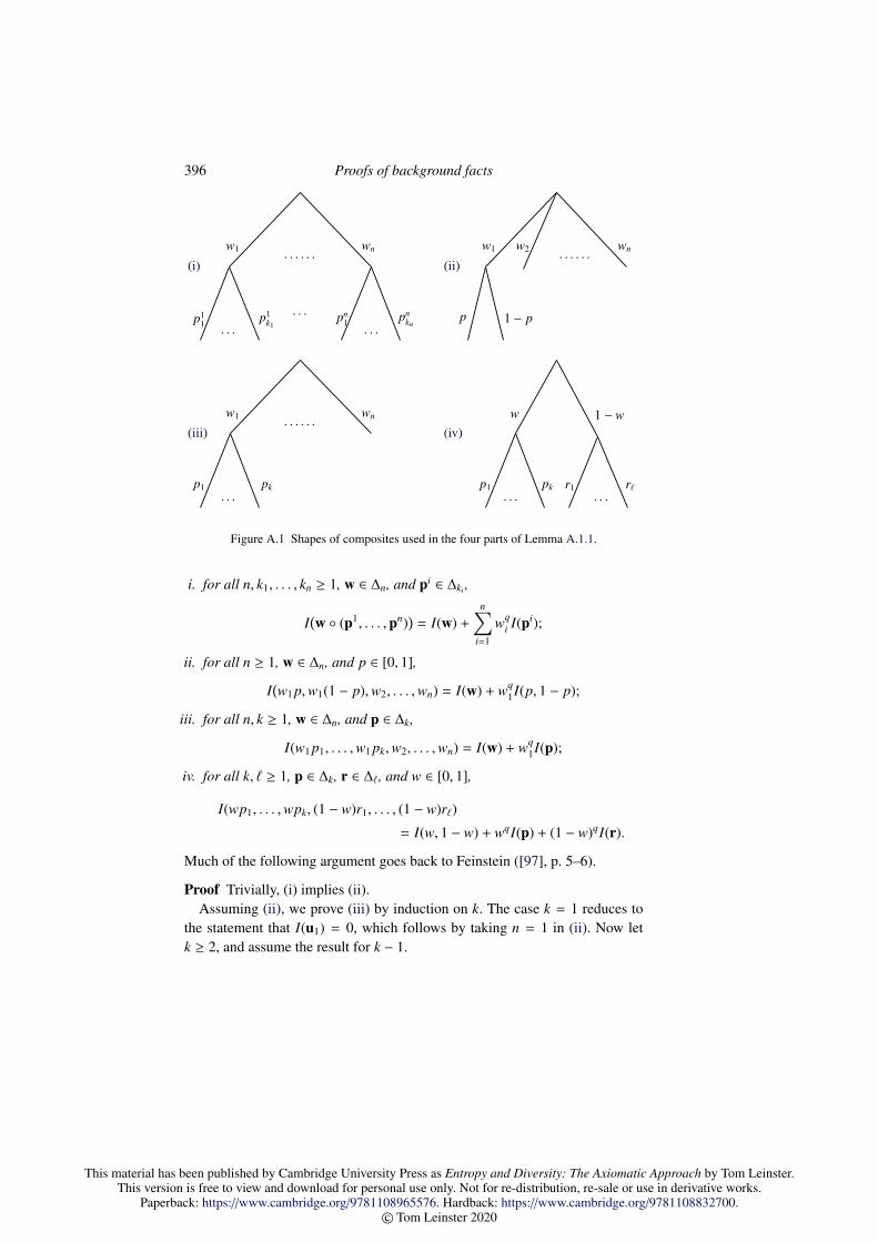
This material has been published by Cambridge University Press as Entropy and Diversity: The Axiomatic Approach by Tom Leinster.This version is free to view and download for personal use only. Not for re-distribution, re-sale or use in derivative works.
Paperback: https://www.cambridge.org/9781108965576. Hardback: https://www.cambridge.org/9781108832700.© Tom Leinster 2020
396 Proofs of background facts
· · · · · ·
· · ·
· · · · · ·
w1 wn
p11 p1
k1pn
1 pnkn
(i)· · · · · ·
w1 w2 wn
p 1 − p
(ii)
· · · · · ·
· · ·
w1 wn
p1 pk
(iii)
· · · · · ·
w 1 − w
p1 pk r1 r`
(iv)
Figure A.1 Shapes of composites used in the four parts of Lemma A.1.1.
i. for all n, k1, . . . , kn ≥ 1, w ∈ ∆n, and pi ∈ ∆ki ,
I(w (p1, . . . ,pn)
)= I(w) +
n∑i=1
wqi I(pi);
ii. for all n ≥ 1, w ∈ ∆n, and p ∈ [0, 1],
I(w1 p,w1(1 − p),w2, . . . ,wn) = I(w) + wq
1I(p, 1 − p);
iii. for all n, k ≥ 1, w ∈ ∆n, and p ∈ ∆k,
I(w1 p1, . . . ,w1 pk,w2, . . . ,wn) = I(w) + wq1I(p);
iv. for all k, ` ≥ 1, p ∈ ∆k, r ∈ ∆`, and w ∈ [0, 1],
I(wp1, . . . ,wpk, (1 − w)r1, . . . , (1 − w)r`)
= I(w, 1 − w) + wqI(p) + (1 − w)qI(r).
Much of the following argument goes back to Feinstein ([97], p. 5–6).
Proof Trivially, (i) implies (ii).Assuming (ii), we prove (iii) by induction on k. The case k = 1 reduces to
the statement that I(u1) = 0, which follows by taking n = 1 in (ii). Now letk ≥ 2, and assume the result for k − 1.
This material has been published by Cambridge University Press as Entropy and Diversity: The Axiomatic Approach by Tom Leinster.This version is free to view and download for personal use only. Not for re-distribution, re-sale or use in derivative works.
Paperback: https://www.cambridge.org/9781108965576. Hardback: https://www.cambridge.org/9781108832700.© Tom Leinster 2020
A.1 Forms of the chain rule for entropy 397
Let n ≥ 1, w ∈ ∆n, and p ∈ ∆k. By symmetry, we can assume that pk < 1.Using the inductive hypothesis, we have
I(w1 p1, . . . ,w1 pk,w2, . . . ,wn)
= I(w1(1 − pk) ·
p1
1 − pk, . . . ,w1(1 − pk) ·
pk−1
1 − pk,w1 pk,w2, . . . ,wn
)= I
(w1(1 − pk),w1 pk,w2, . . . ,wn
)+
(w1(1 − pk)
)qI( p1
1 − pk, . . . ,
pk−1
1 − pk
),
which by (ii) is equal to
I(w) + wq1
I(1 − pk, pk) + (1 − pk)qI
( p1
1 − pk, . . . ,
pk−1
1 − pk
).
But by the inductive hypothesis again, the term · · · is equal to
I((1 − pk) ·
p1
1 − pk, . . . , (1 − pk) ·
pk−1
1 − pk, pk
)= I(p),
completing the induction.Now assuming (iii), we prove (iv). Let k, ` ≥ 1, p ∈ ∆k, r ∈ ∆`, and w ∈
[0, 1]. Using (iii), we have
I(wp1, . . . ,wpk, (1 − w)r1, . . . , (1 − w)r`)
= I(w, (1 − w)r1, . . . , (1 − w)r`
)+ wqI(p).
By symmetry and (iii) again, this in turn is equal to
I(w, 1 − w) + (1 − w)qI(r) + wqI(p),
proving (iv).Finally, assume (iv). We prove (i) by induction on n. The case n = 1 just
states that I(u1) = 0, which follows from (iv) by taking k = ` = 1. Now letn ≥ 2, and assume the result for n − 1.
Let k1, . . . , kn ≥ 1, w ∈ ∆n, and pi ∈ ∆ki . By symmetry, we can assume thatw1 > 0. Write
p12 =
( w1
w1 + w2p1
1, . . . ,w1
w1 + w2p1
k1,
w2
w1 + w2p2
1, . . . ,w2
w1 + w2p2
k2
)∈ ∆k1+k2 .
Then
w (p1, . . . ,pn) = (w1 + w2,w3, . . . ,wn) (p12,p3, . . . ,pn),
This material has been published by Cambridge University Press as Entropy and Diversity: The Axiomatic Approach by Tom Leinster.This version is free to view and download for personal use only. Not for re-distribution, re-sale or use in derivative works.
Paperback: https://www.cambridge.org/9781108965576. Hardback: https://www.cambridge.org/9781108832700.© Tom Leinster 2020
398 Proofs of background facts
so by inductive hypothesis,
I(w (p1, . . . ,pn)
)= I(w1 + w2,w3, . . . ,wn) + (w1 + w2)qI(p12) +
n∑i=3
wqi I(pi). (A.1)
On the other hand, by (iv),
I(p12) = I( w1
w1 + w2,
w2
w1 + w2
)+
( w1
w1 + w2
)qI(p1) +
( w2
w1 + w2
)qI(p2).
Substituting this into (A.1), we deduce that I(w (p1, . . . ,pn)
)is equal to
I(w1 + w2,w3, . . . ,wn) + (w1 + w2)qI( w1
w1 + w2,
w2
w1 + w2
)+
n∑i=1
wqi I(pi). (A.2)
But applying the inductive hypothesis to the composite
w = (w1 + w2,w3, . . . ,wn) (( w1
w1 + w2,
w2
w1 + w2
),u1, . . . ,u1
)gives
I(w) = I(w1 + w2,w3, . . . ,wn) + (w1 + w2)qI( w1
w1 + w2,
w2
w1 + w2
)(recalling that I(u1) = 0). Hence the expression (A.2) reduces to
I(w) +
n∑i=1
wqi I(pi),
proving (i).
A.2 The expected number of species in a random sample
Here we prove the result stated in Example 4.3.6, which expresses the diversityindex of Hurlbert, Smith and Grassle in terms of the Hill numbers Dq(p).
Recall that we are modelling an ecological community with n species via itsrelative abundance distribution, and that HHSG
m (p) denotes the expected numberof different species represented in a random sample with replacement of mindividuals. The claim is that
HHSGm (p) =
m∑q=1
(−1)q−1(mq
)Dq(p)1−q.

This material has been published by Cambridge University Press as Entropy and Diversity: The Axiomatic Approach by Tom Leinster.This version is free to view and download for personal use only. Not for re-distribution, re-sale or use in derivative works.
Paperback: https://www.cambridge.org/9781108965576. Hardback: https://www.cambridge.org/9781108832700.© Tom Leinster 2020
A.3 The diversity profile determines the distribution 399
Define random variables X1, . . . , Xn by
Xi =
1 if species i is present in the sample,
0 otherwise.
Then∑n
i=1 Xi is the number of different species in the sample, so
HHSGm (p) = E
( n∑i=1
Xi
)=
n∑i=1
E(Xi)
=
n∑i=1
Pr(species i is present in the sample)
=
n∑i=1
(1 − (1 − pi)m)
,
as Hurlbert observed (equation (14) of [148]). It follows that
HHSGm (p) = n −
n∑i=1
m∑q=0
(mq
)(−pi)q
= n −m∑
q=0
(−1)q(mq
) n∑i=1
pqi
= n −(
m0
)n −
(m1
)1 +
m∑q=2
(−1)q(mq
)Dq(p)1−q
= m −m∑
q=2
(−1)q(mq
)Dq(p)1−q
=
m∑q=1
(−1)q−1(mq
)Dq(p)1−q,
as claimed.
A.3 The diversity profile determines the distribution
Here we prove the result claimed in Remark 4.4.9: two probability distributionson the same finite set have the same diversity profile if and only if one is apermutation of the other. Formally:

This material has been published by Cambridge University Press as Entropy and Diversity: The Axiomatic Approach by Tom Leinster.This version is free to view and download for personal use only. Not for re-distribution, re-sale or use in derivative works.
Paperback: https://www.cambridge.org/9781108965576. Hardback: https://www.cambridge.org/9781108832700.© Tom Leinster 2020
400 Proofs of background facts
Lemma A.3.1 Let n ≥ 1 and p, r ∈ ∆n. The following are equivalent:
i. Dq(p) = Dq(r) for all q ∈ [−∞,∞];
ii. there exists a subset Q ⊆ [−∞,∞), unbounded above, such that Dq(p) =
Dq(r) for all q ∈ Q;
iii. p = rσ for some permutation σ of 1, . . . , n.
This result first appeared as Proposition A22 of the appendix to Leinster andCobbold [218].
Proof (iii) implies (i) by the symmetry of the Hill numbers (Lemma 4.4.8),and (i) implies (ii) trivially. Now assuming (ii), we prove (iii) by induction onn. It is trivial for n = 1. Let n ≥ 2, assume the result for n−1, and take p, r ∈ ∆n
such that Dq(p) = Dq(r) for all elements q of some set Q ⊆ [−∞,∞) that isunbounded above. We may assume that −∞ < Q and 1 < Q (for if not, removethem).
We know that Dq(p) is continuous in q ∈ [−∞,∞], by Lemma 4.2.7 orLemma 6.2.4(i). Since Q is unbounded above,
limq∈Q, q→∞
Dq(p) = D∞(p) = 1/max1≤i≤n
pi.
The same is true for Dq(r). Hence by assumption, maxi pi = maxi ri. Choose kand ` such that pk = maxi pi and r` = maxi ri. Then pk = r`.
If pk = r` = 1 then p and r are both of the form (0, . . . , 0, 1, 0, . . . , 0), so oneis a permutation of the other. Assuming otherwise, define p′, r′ ∈ ∆n−1 by
p′ =
( p1
1 − pk, . . . ,
pk−1
1 − pk,
pk+1
1 − pk, . . . ,
pn
1 − pk
)and similarly for r′. Then for all q ∈ Q,
Dq(p′) = (1 − pk)q/(q−1)(∑
i,k
pqi
)1/(1−q)
= (1 − pk)q/(q−1)(Dq(p)1−q − pqk)1/(1−q)
.
Similarly,
Dq(r′) = (1 − r`)q/(q−1)(Dq(r)1−q − rq`
)1/(1−q).
But pk = r` and Dq(p) = Dq(r), so Dq(p′) = Dq(r′). This holds for all q ∈ Q,so by inductive hypothesis, p′ is a permutation of r′. It follows that p is apermutation of r, completing the induction.
This material has been published by Cambridge University Press as Entropy and Diversity: The Axiomatic Approach by Tom Leinster.This version is free to view and download for personal use only. Not for re-distribution, re-sale or use in derivative works.
Paperback: https://www.cambridge.org/9781108965576. Hardback: https://www.cambridge.org/9781108832700.© Tom Leinster 2020
A.4 Affine functions 401
A.4 Affine functions
Here we prove Lemma 5.1.7, which is restated here for convenience.
Lemma 5.1.7 Let α : I → J be a function between real intervals. The follow-ing are equivalent:
i. α is affine;ii. α
(∑λixi
)=
∑λiα(xi) for all n ≥ 1, x1, . . . , xn ∈ I and λ1, . . . , λn ∈ R such
that∑λi = 1 and
∑λixi ∈ I;
iii. there exist constants a, b ∈ R such that α(x) = ax + b for all x ∈ I;iv. α is continuous and α
( 12 (x1 + x2)
)= 1
2(α(x1) + α(x2)
)for all x1, x2 ∈ I.
Proof First we assume (i) and prove (ii). By induction,
α
( n∑i=1
pixi
)=
n∑i=1
piα(xi) (A.3)
for all n ≥ 1, p ∈ ∆n, and x ∈ In. Now let n ≥ 1, x1, . . . , xn ∈ I and λ1, . . . , λn ∈
R with∑λi = 1 and
∑λixi ∈ I. Assume without loss of generality that
λ1, . . . , λk ≥ 0, λk+1, . . . , λn < 0
for some k ∈ 1, . . . , n. Write
µ =
k∑i=1
λi = 1 −n∑
i=k+1
λi ≥ 1, w =
n∑i=1
λixi ∈ I.
Thenk∑
i=1
λi
µxi =
1µ
w +
n∑i=k+1
−λi
µxi.
The coefficients λ1/µ, . . . , λk/µ on the left-hand side are nonnegative and sumto 1, and the same is true of the coefficients 1/µ,−λk+1/µ, . . . ,−λn/µ on theright-hand side. Hence we can apply α throughout and use equation (A.3) onboth sides, giving
k∑i=1
λi
µα(xi) =
1µα(w) +
n∑i=k+1
−λi
µα(xi).
Rearranging gives
α(w) =
n∑i=1
λiα(xi),
proving (ii).

This material has been published by Cambridge University Press as Entropy and Diversity: The Axiomatic Approach by Tom Leinster.This version is free to view and download for personal use only. Not for re-distribution, re-sale or use in derivative works.
Paperback: https://www.cambridge.org/9781108965576. Hardback: https://www.cambridge.org/9781108832700.© Tom Leinster 2020
402 Proofs of background facts
Next we assume (ii) and prove (iii). If I is trivial, the result is trivial. Other-wise, we can choose distinct x1, x2 ∈ I. Put
a =α(x2) − α(x1)
x2 − x1, b =
α(x1)x2 − α(x2)x1
x2 − x1,
and define α′ : R → R by α′(x) = ax + b. We show that α(x) = α′(x) for allx ∈ I. First, this is true when x ∈ x1, x2, by direct calculation. Second, everyelement of I can be written as λ1x1 +λ2x2 for some λ1, λ2 ∈ Rwith λ1 +λ2 = 1.Since both α and α′ satisfy (ii), the result follows.
Trivially, (iii) implies (iv).Finally, assuming (iv), we prove (i). By continuity, it is enough to prove that
α(px1 + (1 − p)x2
)= pα(x1) + (1 − p)α(x2)
whenever x1, x2 ∈ I and p ∈ [0, 1] is a dyadic rational, that is, p = m/2n forsome integers n ≥ 0 and 0 ≤ m ≤ 2n. We do this by induction on n. It is trivialfor n = 0. Now let n ≥ 1 and assume the result for n − 1. Let x1, x2 ∈ I, let0 ≤ m ≤ 2n, and assume without loss of generality that m ≤ 2n−1 (otherwisewe can reverse the roles of x1 and x2). Then
α
(m2n x1 +
(1 −
m2n
)x2
)= α
(m
2n−1 ·12
(x1 + x2) +
(1 −
m2n−1
)x2
)(A.4)
=m
2n−1α(12
(x1 + x2))
+
(1 −
m2n−1
)α(x2) (A.5)
=m
2n−1 ·12(α(x1) + α(x2)
)+
(1 −
m2n−1
)α(x2) (A.6)
=m2nα(x1) +
(1 −
m2n
)α(x2), (A.7)
where (A.4) and (A.7) are elementary, (A.5) is by inductive hypothesis,and (A.6) is by (iv). This completes the induction and, therefore, the proof.
A.5 Diversity of integer orders
Here we prove the statement made in Example 6.1.7 on computation of thediversity DZ
q (p) for integers q ≥ 2: that in the notation defined there,
DZq (p) = µ
1/(1−q)q .
This material has been published by Cambridge University Press as Entropy and Diversity: The Axiomatic Approach by Tom Leinster.This version is free to view and download for personal use only. Not for re-distribution, re-sale or use in derivative works.
Paperback: https://www.cambridge.org/9781108965576. Hardback: https://www.cambridge.org/9781108832700.© Tom Leinster 2020
A.6 The maximum entropy of a coupling 403
Indeed, adopting the convention that all sums run over 1, . . . , n,
DZq (p)1−q =
∑i
pi
(∑j
Zi j p j
)q−1
=∑
i, j1,..., jq−1
piZi j1 p j1 Zi j2 p j2 · · · Zi jq−1 p jq−1
=∑
i1,i2,...,iq
pi1 pi2 · · · piq Zi1i2 Zi1i3 · · · Zi1iq
= µq,
as required.
A.6 The maximum entropy of a coupling
Let p and r be probability distributions on finite setsX andY, respectively. Weshowed in Remark 8.1.13 that among all distributions onX×Y with marginalsp and r, none has greater entropy than p ⊗ r. In other words,
H(P) ≤ H(p ⊗ r) (A.8)
for all probability distributions P on X×Y whose marginal distributions are pand r. It was also claimed there that unless q = 0 or q = 1, the inequality (A.8)fails when H is replaced by the Renyi entropy Hq or the q-logarithmic entropyS q. Here we prove this claim.
Since Hq and S q are increasing, invertible transformations of one another,it suffices to prove it for Hq. And since Renyi entropy is logarithmic (equa-tion (4.14)), the inequality in question can be restated as
Hq(P) ≤ Hq(p) + Hq(r). (A.9)
This is true for q = 0:
supp(P) ⊆ supp(p) × supp(r),
so
|supp(P)| ≤ |supp(p)| · |supp(r)|,
giving
H0(P) = log|supp(P)| ≤ log|supp(p)| + log|supp(r)| = H0(p) + H0(r).
Our task now is to show that except in the cases q = 0 and q = 1, the inequal-ity (A.9) is false. Thus, we prove that for each q ∈ (0, 1) ∪ (1,∞], there exist
This material has been published by Cambridge University Press as Entropy and Diversity: The Axiomatic Approach by Tom Leinster.This version is free to view and download for personal use only. Not for re-distribution, re-sale or use in derivative works.
Paperback: https://www.cambridge.org/9781108965576. Hardback: https://www.cambridge.org/9781108832700.© Tom Leinster 2020
404 Proofs of background facts
finite sets X and Y and a probability distribution P on X ×Y such that
Hq(P) > Hq(p) + Hq(r),
where p and r are the marginal distributions of P.We will treat separately the cases q ∈ (0, 1), q ∈ (1,∞), and q = ∞. In all
cases, we will take X = Y = 1, . . . ,N for some N. A probability distributionP on X×Y is then an N ×N matrix of nonnegative real numbers whose entriessum to 1, and its marginals p and r are given by the row-sums and column-sums:
pi =
N∑j=1
Pi j, r j =
N∑i=1
Pi j
(i, j ∈ 1, . . . ,N).First let q ∈ (0, 1). For each N ≥ 2, define an N × N matrix P by
P =
1 − (N − 1)(q−1)/q 0 · · · 0
0 (N − 1)(−q−1)/q · · · (N − 1)(−q−1)/q
......
...
0 (N − 1)(−q−1)/q · · · (N − 1)(−q−1)/q
.The entries of P sum to 1, and 1−(N−1)(q−1)/q ≥ 0 since q ∈ (0, 1), so P ∈ ∆N2 .We have
Hq(P) =1
1 − qlog
((1 − (N − 1)(q−1)/q)q
+ (N − 1)2(N − 1)−q−1)
≥1
1 − qlog
((N − 1)−q+1)
= log(N − 1).
The marginals of P are
p = r =(1 − (N − 1)(q−1)/q, (N − 1)−1/q, . . . , (N − 1)−1/q︸ ︷︷ ︸
N−1
),
so
Hq(p) = Hq(r) =1
1 − qlog
((1 − (N − 1)(q−1)/q)q
+ (N − 1) · (N − 1)−1)
<1
1 − qlog 2.
Hence
Hq(P) −(Hq(p) + Hq(r)
)> log(N − 1) −
21 − q
log 2→ ∞

This material has been published by Cambridge University Press as Entropy and Diversity: The Axiomatic Approach by Tom Leinster.This version is free to view and download for personal use only. Not for re-distribution, re-sale or use in derivative works.
Paperback: https://www.cambridge.org/9781108965576. Hardback: https://www.cambridge.org/9781108832700.© Tom Leinster 2020
A.6 The maximum entropy of a coupling 405
as N → ∞. In particular, Hq(P) > Hq(p) + Hq(r) when N is sufficiently large.Now let q ∈ (1,∞). For each N ≥ 2, define an N × N matrix P by
P =
0 1/2(N − 1) · · · 1/2(N − 1)
1/2(N − 1) 0 · · · 0...
......
1/2(N − 1) 0 · · · 0
.The entries of P are nonnegative and sum to 1, and
Hq(P) = Hq(u2(N−1)) = log(2(N − 1)
)→ ∞
as N → ∞. The marginals of P are
p = r =(1/2, 1/2(N − 1), . . . , 1/2(N − 1)︸ ︷︷ ︸
N−1
),
and
Hq(p) = Hq(r) =1
1 − qlog
((1/2)q + (N − 1) ·
(1/2(N − 1)
)q)
=1
1 − qlog
((1/2)q) +
11 − q
log(1 + (N − 1)1−q)
→1
1 − qlog
((1/2)q)
as N → ∞, since q > 1. Hence
Hq(P) −(Hq(p) + Hq(r)
)→ ∞
as N → ∞, which again implies that Hq(P) > Hq(p) + Hq(r) when N is suffi-ciently large.
Finally, let q = ∞. The same matrix P as in the previous case has
H∞(P) = log(2(N − 1)
),
H∞(p) = H∞(r) = log 2.
Hence
H∞(P) −(H∞(p) + H∞(r)
)= log
(2(N − 1)
)− 2 log 2→ ∞
as N → ∞. Once again, this implies that H∞(P) > H∞(p) + H∞(r) for suffi-ciently large N.
This material has been published by Cambridge University Press as Entropy and Diversity: The Axiomatic Approach by Tom Leinster.This version is free to view and download for personal use only. Not for re-distribution, re-sale or use in derivative works.
Paperback: https://www.cambridge.org/9781108965576. Hardback: https://www.cambridge.org/9781108832700.© Tom Leinster 2020
406 Proofs of background facts
A.7 Convex duality
Here we prove Theorem 9.2.7, which is restated here for convenience.
Theorem 9.2.7 (Legendre–Fenchel) Let f : R → R be a convex function.Then f ∗∗ = f .
Proof Let x ∈ R. By definition of convex conjugate,
f ∗∗(x) = supλ∈R
(λx − f ∗(λ)
)= sup
λ∈Rinfy∈R
(λ(x − y) + f (y)
). (A.10)
In particular,
f ∗∗(x) ≤ supλ∈R
(λ(x − x) + f (x)
)= f (x),
so it remains to prove that f ∗∗(x) ≥ f (x). In fact, we will show that there existsλ ∈ R such that
λ(x − y) + f (y) ≥ f (x) for all y ∈ R. (A.11)
By (A.10), this will suffice. Now, a real number λ satisfies (A.11) if and onlyif
supy∈(−∞,x)
f (x) − f (y)x − y
≤ λ ≤ infz∈(x,∞)
f (z) − f (x)z − x
,
so such a λ exists if and only if
f (x) − f (y)x − y
≤f (z) − f (x)
z − x(A.12)
for all y < x < z. We now prove this. Take y and z such that y < x < z. Thenx = py + (1 − p)z for some p ∈ (0, 1), and the inequality (A.12) to be provedstates that
f (x) − f (y)(1 − p)(z − y)
≤f (z) − f (x)
p(z − y),
or equivalently,
f (x) ≤ p f (y) + (1 − p) f (z).
This is true by convexity of f .

This material has been published by Cambridge University Press as Entropy and Diversity: The Axiomatic Approach by Tom Leinster.This version is free to view and download for personal use only. Not for re-distribution, re-sale or use in derivative works.
Paperback: https://www.cambridge.org/9781108965576. Hardback: https://www.cambridge.org/9781108832700.© Tom Leinster 2020
A.8 Cumulant generating functions are convex 407
A.8 Cumulant generating functions are convex
In Section 9.2, we used the fact that the cumulant generating function of anyreal random variable is convex. Here we prove this.
If we are willing to assume that the cumulant generating function is twicedifferentiable, then the result can be deduced from the Cauchy–Schwarz in-equality, as in Section 5.11 of Grimmett and Stirzaker [128]. But there is noneed to make this assumption. Instead, we use a more general standard inequal-ity:
Theorem A.8.1 (Holder’s inequality) Let Ω be a measure space, let p, q ∈(1,∞) with 1/p + 1/q = 1, and let f , g : Ω → [0,∞) be measurable functions.Then ∫
Ω
f g ≤(∫
Ω
f p)1/p(∫
Ω
gq)1/q
.
Here we allow the possibility that one or more of the integrals is∞.
Proof This is Theorem 6.2 of Folland [106], for instance.
Corollary A.8.2 Let X be a real random variable. Then the function
R → [0,∞]λ 7→ logE(eλX)
is convex.
Proof We have to prove that for all λ, µ ∈ R and t ∈ [0, 1],
logE(e(tλ+(1−t)µ)X
)≤ t logE
(eλX) + (1 − t) logE
(e µX),
or equivalently,
E(etλXe(1−t)µX
)≤ E
(eλX)t
E(e µX)1−t
.
This is trivial if t = 0 or t = 1. Supposing otherwise, write p = 1/t, q =
1/(1 − t), U = etλX , and V = e(1−t)µX . Thus, p, q ∈ (1,∞) with 1/p + 1/q = 1,and U and V are nonnegative real random variables on the same sample space.The inequality to be proved is that
E(UV) ≤ E(U p)1/p E(Vq)1/q,
which is just Holder’s inequality in probabilistic notation.
This material has been published by Cambridge University Press as Entropy and Diversity: The Axiomatic Approach by Tom Leinster.This version is free to view and download for personal use only. Not for re-distribution, re-sale or use in derivative works.
Paperback: https://www.cambridge.org/9781108965576. Hardback: https://www.cambridge.org/9781108832700.© Tom Leinster 2020
408 Proofs of background facts
A.9 Functions on a finite field
Here we prove Lemma 11.4.1, which is restated here for convenience.
Lemma 11.4.1 Let K be a finite field with q elements, let n ≥ 0, and letF : Kn → K be a function. Then there is a unique polynomial f of the form
f (x1, . . . , xn) =∑
0≤r1,...,rn<q
cr1,...,rn xr11 · · · x
rnn (A.13)
(cr1,...,rn ∈ K) such that
f (π1, . . . , πn) = F(π1, . . . , πn)
for all π1, . . . , πn ∈ K.
This result is standard. For instance, Section 10.3 of Roman [297] gives aproof in the case n = 1.
Proof Write K<q[x1, . . . , xn] for the set of polynomials of degree less than q ineach variable, that is, of the form (A.13). Write R( f ) : Kn → K for the functioninduced by a polynomial f in n variables. Then R defines a map
R : K<q[x1, . . . , xn]→ functions Kn → K.
We have to prove that R is bijective. Both domain and codomain have qqn
elements, so it suffices to prove that R is surjective.First define a polynomial δ by
δ(x1, . . . , xn) = (1 − xq−11 ) · · · (1 − xq−1
n ).
Then δ has degree q − 1 in each variable, and for a1, . . . , an ∈ K,
R(δ)(a1, . . . , an) =
1 if a1 = · · · = an = 0,
0 otherwise.
Now, given a function F : Kn → K, define a polynomial f by
f (x1, . . . , xn) =∑
a1,...,an∈K
F(a1, . . . , an)δ(x1 − a1, . . . , xn − an).
Then f has degree at most q − 1 in each variable and R( f ) = F, as required.
There are other proofs. For instance, one can prove that R is injective ratherthan surjective, showing by induction on n that its kernel is trivial. I thank ToddTrimble for pointing out to me the Lagrange interpolation argument above.

This material has been published by Cambridge University Press as Entropy and Diversity: The Axiomatic Approach by Tom Leinster.This version is free to view and download for personal use only. Not for re-distribution, re-sale or use in derivative works.
Paperback: https://www.cambridge.org/9781108965576. Hardback: https://www.cambridge.org/9781108832700.© Tom Leinster 2020
Appendix B
Summary of conditions
Here we list the main conditions on means, diversity measures and value mea-sures used in the text. For each condition, we give an abbreviated form of thedefinition and a reference to the point(s) in the text where it is defined in full.
Weighted means
The following conditions apply to a sequence(M : ∆n×In → I
)n≥1 of functions,
where I is a real interval. For the homogeneity and multiplicativity conditions,I is assumed to be closed under multiplication.
Name Abbreviated definition Reference
Absence- M((. . . , pi−1, 0, pi+1), (. . . , xi−1, xi, xi+1, . . .))invariant = M((. . . , pi−1, pi+1, . . .), (. . . , xi−1, xi+1, . . .)) Def 4.2.10
Chain rule M(w (p1, . . . ,pn), x1 ⊕ · · · ⊕ xn)= M(w, (M(p1, x1), . . . ,M(pn, xn))) Def 4.2.23
Consistent M(p, (x, . . . , x)) = x Def 4.2.16
Convex M(p, 12 (x + y)) ≤ maxM(p, x),M(p, y) Def 9.4.1
Homogeneous M(p, cx) = cM(p, x) Def 4.2.21
Increasing x ≤ y =⇒ M(p, x) ≤ M(p, y) Def 4.2.18
Modular M(w (p1, . . . ,pn), x1 ⊕ · · · ⊕ xn) depends
only on w and M(p1, x1), . . . ,M(pn, xn) Def 4.2.25
Multiplicative M(p ⊗ p′, x ⊗ x′) = M(p, x)M(p′, x′) Def 4.2.27
Natural M( f p, x) = M(p, x f ) Def 4.2.12
Quasiarithmetic M(p, x) = φ−1(∑ piφ(xi))
for some φ Def 5.1.1
409

This material has been published by Cambridge University Press as Entropy and Diversity: The Axiomatic Approach by Tom Leinster.This version is free to view and download for personal use only. Not for re-distribution, re-sale or use in derivative works.
Paperback: https://www.cambridge.org/9781108965576. Hardback: https://www.cambridge.org/9781108832700.© Tom Leinster 2020
410 Summary of conditions
Repetition M((. . . , pi, pi+1, . . .), (. . . , xi, xi, . . .))= M((. . . , pi + pi+1, . . .), (. . . , xi, . . .)) Def 4.2.10
Strictly increasing x ≤ y and xi < yi for some i ∈ supp(p)=⇒ M(p, x) < M(p, y) Def 4.2.18
Symmetric M(p, x) = M(pσ, xσ) Def 4.2.10
Unweighted means
The following conditions apply to a sequence(M : In → I
)n≥1 of functions,
where I is a real interval. For the homogeneity and multiplicativity conditions,I is assumed to be closed under multiplication.
Name Abbreviated definition Reference
Consistent M(x, . . . , x) = x Def 5.2.3
Decomposable M(x1
1, . . . , x1k1, . . . , xn
1, . . . , xnkn
)= M(a1, . . . , a1, . . . , an, . . . , an)where ai = M
(xi
1, . . . , xiki
)Def 5.2.9
Homogeneous M(cx) = cM(x) Def 5.2.13
Increasing x ≤ y =⇒ M(x) ≤ M(y) Def 5.2.5
Modular M(x1
1, . . . , x1k1, . . . , xn
1, . . . , xnkn
)depends only on k1, . . . , kn andM
(x1
1, . . . , x1k1
), . . . ,M
(xn
1, . . . , xnkn
)Def 5.2.12
Multiplicative M(x ⊗ y) = M(x)M(y) Def 5.2.18
Quasiarithmetic M(x) = φ−1(∑ 1nφ(xi)
)for some φ p. 140
Strictly increasing x ≤ y , x =⇒ M(x) < M(y) Def 5.2.5
Symmetric M(x) = M(xσ) Def 5.2.1
Diversity measures
The following conditions apply to a sequence(D : ∆n → (0,∞)
)n≥1 of func-
tions, that is, a diversity measure for communities modelled as finite probabil-ity distributions (without incorporating species similarity).

This material has been published by Cambridge University Press as Entropy and Diversity: The Axiomatic Approach by Tom Leinster.This version is free to view and download for personal use only. Not for re-distribution, re-sale or use in derivative works.
Paperback: https://www.cambridge.org/9781108965576. Hardback: https://www.cambridge.org/9781108832700.© Tom Leinster 2020
Summary of conditions 411
Name Abbreviated definition Reference
Absence-invariant D(. . . , pi−1, 0, pi+1, . . .)= D(. . . , pi−1, pi+1, . . .) Def 4.4.7
Continuous D : ∆n → (0,∞) is continuous Def 4.4.5
Continuous inpositive probabilities D : ∆n → (0,∞) is continuous Def 4.4.5
Effective number D(un) = n Def 2.4.5
Modular D(w (p1, . . . ,pn)) depends p. 56,only on w and D(p1), . . . ,D(pn) Def 4.4.14
Modular-monotone D(pi) ≤ D(pi) for all i =⇒
D(w(p1, . . . ,pn)) ≤ D(w (p1, . . . , pn)) Def 7.4.1
Multiplicative D(p ⊗ r) = D(p)D(r) Def 4.4.16
Normalized D(u1) = 1 p. 246
Replication principle D(un ⊗ p) = nD(p) p. 56,Def 4.4.18
Symmetric D(p) = D(pσ) p. 96
Value measures
The following conditions apply to a sequence(σ : ∆n × (0,∞)n → (0,∞)
)n≥1
of functions. Such a sequence is of the same type as a weighted mean on(0,∞), and the same terminology applies. We also use two further conditions.
Name Abbreviated definition Reference
Continuous in
positive probabilities σ(−, v) : ∆n → (0,∞) is continuous Def 7.3.1
Effective number σ(un, (1, . . . , 1)) = n Def 7.3.2
This material has been published by Cambridge University Press as Entropy and Diversity: The Axiomatic Approach by Tom Leinster.This version is free to view and download for personal use only. Not for re-distribution, re-sale or use in derivative works.
Paperback: https://www.cambridge.org/9781108965576. Hardback: https://www.cambridge.org/9781108832700.© Tom Leinster 2020
References
[1] J. Aczel. On mean values. Bulletin of the American Mathematical Society,54(4):392–400, 1948.
[2] J. Aczel. Lectures on Functional Equations and their Applications. AcademicPress, New York, 1966.
[3] J. Aczel and Z. Daroczy. On Measures of Information and Their Characteriza-tions, volume 115 of Mathematics in Science and Engineering. Academic, NewYork, 1975.
[4] R. L. Adler, A. G. Konheim, and M. H. McAndrew. Topological entropy. Trans-actions of the American Mathematical Society, 114:309–319, 1965.
[5] J. Aitchison. Simplicial inference. In M. A. G. Viana and D. S. P. Richards,editors, Algebraic Methods in Statistics and Probability, volume 287 of Contem-porary Mathematics, pages 1–22. American Mathematical Society, 2001.
[6] S. Alesker. Theory of valuations on manifolds: a survey. Geometric and Func-tional Analysis, 17:1321–1341, 2007.
[7] S. Alesker, S. Artstein-Avidan, and V. Milman. Characterization of the Fouriertransform and related topics. Comptes Rendus Mathematique Academie des Sci-ences. Paris, 346:625–628, 2008.
[8] S. Alesker and J. H. G. Fu. Integral Geometry and Valuations. Advanced Coursesin Mathematics CRM Barcelona. Birkhauser, Basel, 2014.
[9] L. Alseda, J. Llibre, and M. Misiurewicz. Combinatorial Dynamics and Entropyin Dimension One, volume 5 of Advanced Series in Nonlinear Dynamics. WorldScientific, 2nd edition, 2000.
[10] S. Amari. Differential geometry of curved exponential families—curvatures andinformation loss. The Annals of Statistics, 10(2):357–385, 1982.
[11] S. Amari. A foundation of information geometry. Electronics and Communica-tions in Japan, 66-A(6):1–10, 1983.
[12] S. Amari. Information Geometry and its Applications, volume 194 of AppliedMathematical Sciences. Springer, Japan, 2016.
[13] S. Amari and H. Nagaoka. Methods of Information Geometry, volume 191 ofTranslations of Mathematical Monographs. Oxford University Press, 1993.
[14] M. Ancrenaz, M. Gumal, A. J. Marshall, E. Meijaard, S. A. Wich, andS. Husson. Pongo pygmaeus. The IUCN Red List of Threatened Speciese.T17975A17966347, 2016.
412

This material has been published by Cambridge University Press as Entropy and Diversity: The Axiomatic Approach by Tom Leinster.This version is free to view and download for personal use only. Not for re-distribution, re-sale or use in derivative works.
Paperback: https://www.cambridge.org/9781108965576. Hardback: https://www.cambridge.org/9781108832700.© Tom Leinster 2020
References 413
[15] T. M. Apostol. Mathematical Analysis. Addison-Wesley, Reading, Mas-sachusetts, 1957.
[16] T. M. Apostol. Introduction to Analytic Number Theory. Undergraduate Textsin Mathematics. Springer, 1976.
[17] S. Arimoto. Information measures and capacity of order α for discrete memo-ryless channels. In Topics in Information Theory—2nd Colloquium, Keszthely,Hungary, 1975, pages 41–52. North-Holland, Amsterdam, 1977.
[18] V. I. Arnold. Mathematical Methods of Classical Mechanics, volume 60 ofGraduate Texts in Mathematics. Springer, 2nd edition, 1989.
[19] Y. Asao. Magnitude homology of geodesic metric spaces with an upper curvaturebound. Algebraic & Geometric Topology, to appear, 2021.
[20] G. Aubrun and I. Nechita. The multiplicative property characterizes `p and Lp
norms. Confluentes Mathematici, 3:637–647, 2011.[21] T. Avery. Structure and Semantics. PhD thesis, University of Edinburgh, 2017.[22] N. Ay, J. Jost, H. V. Le, and L. Schwachhofer. Information Geometry, volume 64
of Ergebnisse der Mathematik und ihrer Grenzgebiete. Springer, 2017.[23] J. Baez and J. Dolan. From finite sets to Feynman diagrams. In Mathematics
Unlimited—2001 and Beyond. Springer, Berlin, 2001.[24] J. Baez and T. Fritz. A Bayesian characterization of relative entropy. Theory and
Applications of Categories, 29:421–456, 2014.[25] J. Baez, T. Fritz, and T. Leinster. A characterization of entropy in terms of
information loss. Entropy, 13:1945–1957, 2011.[26] M. G. Bakker, J. M. Chaparro, D. K. Manter, and J. M. Vivanco. Impacts of bulk
soil microbial community structure on rhizosphere microbiomes of Zea mays.Plant Soil, 392:115–126, 2015.
[27] S. Banach. Sur l’equation fonctionnelle f (x + y) = f (x) + f (y). FundamentaMathematicae, 1:123–124, 1920.
[28] J. A. Barcelo and A. Carbery. On the magnitudes of compact sets in Euclideanspaces. American Journal of Mathematics, 140(2):449–494, 2018.
[29] A. R. Barron. Entropy and the central limit theorem. The Annals of Probability,14(1):336–342, 1986.
[30] B. H. Barton and E. Moran. Measuring diversity on the Supreme Court withbiodiversity statistics. Journal of Empirical Legal Studies, 10:1–34, 2013.
[31] M. A. Batanin. The Eckmann–Hilton argument and higher operads. Advancesin Mathematics, 217:334–385, 2008.
[32] P. Baudot and D. Bennequin. The homological nature of entropy. Entropy,17:3253–3318, 2015.
[33] C. Beck and F. Schlogl. Thermodynamics of Chaotic Systems: An Introduction,volume 4 of Cambridge Nonlinear Science Series. Cambridge University Press,1993.
[34] J. Benabou. Introduction to bicategories. In J. Benabou, R. Davis, A. Dold,S. Mac Lane, J. Isbell, U. Oberst, and J.-E. Roos, editors, Reports of the MidwestCategory Seminar, Lecture Notes in Mathematics 47. Springer, Berlin, 1967.
[35] A. Berarducci, P. Majer, and M. Novaga. Infinite paths and cliques in randomgraphs. Fundamenta Mathematicae, 216:163–191, 2012.
[36] P. Berezinski, B. Jasiul, and M. Szpyrka. An entropy-based network anomalydetection method. Entropy, 17:2367–2408, 2015.
This material has been published by Cambridge University Press as Entropy and Diversity: The Axiomatic Approach by Tom Leinster.This version is free to view and download for personal use only. Not for re-distribution, re-sale or use in derivative works.
Paperback: https://www.cambridge.org/9781108965576. Hardback: https://www.cambridge.org/9781108832700.© Tom Leinster 2020
414 References
[37] C. Berger and T. Leinster. The Euler characteristic of a category as the sum of adivergent series. Homology, Homotopy and Applications, 10(1):41–51, 2008.
[38] W. H. Berger and F. L. Parker. Diversity of planktonic Foraminifera in deep-seasediments. Science, 168:1345–1347, 1970.
[39] A. Bhattacharyya. On a measure of divergence between two statistical popula-tions defined by their probability distribution. Bulletin of the Calcutta Mathe-matical Society, 35(1):99–109, 1943.
[40] R. L. Bishop. Elasticities, cross-elasticities, and market relationships. The Amer-ican Economic Review, 42(5):780–803, 1952.
[41] R. Blackwell, G. M. Kelly, and A. J. Power. Two-dimensional monad theory.Journal of Pure and Applied Algebra, 59:1–41, 1989.
[42] A. Blass and Y. Gurevich. Negative probability. Bulletin of the European Asso-ciation for Theoretical Computer Science, 115:126–142, 2015.
[43] A. Blass and Y. Gurevich. Negative probabilities, II: What they are and what theyare for. Bulletin of the European Association for Theoretical Computer Science,125:152–168, 2018.
[44] J. M. Boardman and R. Vogt. Homotopy Invariant Algebraic Structures on Topo-logical Spaces, volume 347 of Lecture Notes in Mathematics. Springer, 1973.
[45] F. Borceux. Handbook of Categorical Algebra 2: Categories and Structures,volume 51 of Encyclopedia of Mathematics and its Applications. CambridgeUniversity Press, 1994.
[46] A. Borgoo, P. Jaque, A. Toro-Labbe, C. V. Alsenoy, and P. Geerlings. AnalyzingKullback–Leibler information profiles: an indication of their chemical relevance.Physical Chemistry Chemical Physics, 11:476–482, 2009.
[47] J. M. Borwein and A. S. Lewis. Convex Analysis and Nonlinear Optimization:Theory and Examples. Canadian Mathematical Society Books in Mathematics.Springer, New York, 2000.
[48] A. Boularias, J. Kober, and J. Peters. Relative entropy inverse reinforcementlearning. In G. Gordon, D. Dunson, and M. Dudık, editors, Proceedings ofthe Fourteenth International Conference on Artificial Intelligence and Statistics,volume 15 of Proceedings of Machine Learning Research, pages 182–189, FortLauderdale, FL, USA, 11–13 Apr 2011.
[49] G. E. P. Box and D. R. Cox. An analysis of transformations. Journal of the RoyalStatistical Society. Series B (Methodological), 26:211–252, 1964.
[50] J. F. Bromaghin, K. D. Rode, S. M. Budge, and G. W. Thiemann. Distancemeasures and optimization spaces in quantitative fatty acid signature analysis.Ecology and Evolution, 5:1249–1262, 2015.
[51] B. Buck and V. A. Macaulay, editors. Maximum Entropy in Action. OxfordUniversity Press, Oxford, 1991.
[52] D. Buck and E. Flapan. Predicting knot or catenane type of site-specific recom-bination products. Journal of Molecular Biology, 374:1186–1199, 2007.
[53] D. Buck and E. Flapan. A topological characterization of knots and links aris-ing from site-specific recombination. Journal of Physics A: Mathematical andTheoretical, 40:12377–12395, 2007.
[54] A. Buium. Differential characters of abelian varieties over p-adic fields. Inven-tiones Mathematicae, 122:309–340, 1995.
This material has been published by Cambridge University Press as Entropy and Diversity: The Axiomatic Approach by Tom Leinster.This version is free to view and download for personal use only. Not for re-distribution, re-sale or use in derivative works.
Paperback: https://www.cambridge.org/9781108965576. Hardback: https://www.cambridge.org/9781108832700.© Tom Leinster 2020
References 415
[55] A. Buium. Arithmetic analogues of derivations. Journal of Algebra, 198:290–299, 1997.
[56] M. A. Buzas and T. G. Gibson. Species diversity: benthonic Foraminifera inwestern North Atlantic. Science, 163:72–75, 1969.
[57] J. W. Cannon and W. J. Floyd. What is. . . Thompson’s group? Notices of theAmerican Mathematical Society, 58(8):1112–1113, 2011.
[58] J. W. Cannon, W. J. Floyd, and W. R. Parry. Introductory notes on RichardThompson’s groups. L’Enseignement Mathematique, 42:215–256, 1996.
[59] G. Carlsson. Topology and data. Bulletin of the American Mathematical Society,46(2):255–308, 2009.
[60] J.-L. Cathelineau. Sur l’homologie de SL2 a coefficients dans l’action adjointe.Mathematica Scandinavica, 63:51–86, 1988.
[61] J.-L. Cathelineau. Remarques sur les differentielles des polylogarithmes uni-formes. Annales de l’Institut Fourier, 46:1327–1347, 1996.
[62] R. Cerf and P. Petit. Short proof of Cramer’s theorem in R. American Mathe-matical Monthly, pages 925–931, December 2011.
[63] S. R. Chakravarty and W. Eichhorn. An axiomatic characterization of a gener-alized index of concentration. The Journal of Productivity Analysis, 2:103–112,1991.
[64] L. Chalmandrier, T. Munkemuller, S. Lavergne, and W. Thuiller. Effects ofspecies’ similarity and dominance on the functional and phylogenetic structureof a plant meta-community. Ecology, 96:143–153, 2015.
[65] A. Chao, C.-H. Chiu, and L. Jost. Phylogenetic diversity measures based on Hillnumbers. Philosophical Transactions of the Royal Society B, 365:3599–3609,2010.
[66] S. Cho. Quantales, persistence, and magnitude homology. PreprintarXiv:1910.02905, available at arXiv.org, 2019.
[67] J. Chuang, A. King, and T. Leinster. On the magnitude of a finite dimensionalalgebra. Theory and Applications of Categories, 31:63–72, 2016.
[68] K.-S. Chung, W.-S. Chung, S.-T. Nam, and H.-J. Kang. New q-derivative andq-logarithm. International Journal of Theoretical Physics, 33:2019–2029, 1994.
[69] T. M. Cover and J. A. Thomas. Elements of Information Theory. John Wiley &Sons, New York, 1st edition, 1991.
[70] H. Cramer. Mathematical Methods of Statistics. Princeton University Press,Princeton, New Jersey, 1946.
[71] N. Cressie and T. R. C. Read. Multinomial goodness-of-fit tests. Journal of theRoyal Statistical Society. Series B (Methodological), 46(3):440–464, 1984.
[72] I. Csiszar. Generalized cutoff rates and Renyi’s information measures. IEEETransactions on Information Theory, 41(1):26–34, 1995.
[73] I. Csiszar. Axiomatic characterizations of information measures. Entropy,10:261–273, 2008.
[74] I. Csiszar and P. C. Shields. Information theory and statistics: a tutorial. Foun-dations and Trends in Communications and Information Theory, 1(4):417–528,2004.

This material has been published by Cambridge University Press as Entropy and Diversity: The Axiomatic Approach by Tom Leinster.This version is free to view and download for personal use only. Not for re-distribution, re-sale or use in derivative works.
Paperback: https://www.cambridge.org/9781108965576. Hardback: https://www.cambridge.org/9781108832700.© Tom Leinster 2020
416 References
[75] F. Dahlqvist, V. Danos, I. Garnier, and O. Kammar. Bayesian inversion by ω-complete cone duality. In J. Desharnais and R. Jagadeesan, editors, 27th In-ternational Conference on Concurrency Theory (CONCUR 2016), pages 1–15.Schloss Dagstuhl–Leibniz-Zentrum fur Informatik, 2016.
[76] Z. Daroczy. Generalized information functions. Information and Control, 16:36–51, 1970.
[77] P.-T. De Boer, D. P. Kroese, S. Mannor, and R. Y. Rubinstein. A tutorial on thecross-entropy method. Annals of Operations Research, 134:19–67, 2005.
[78] C. Dellacherie and P.-A. Meyer. Probabilities and Potential, C: Potential Theoryfor Discrete and Continuous Semigroups, volume 151 of North-Holland Mathe-matics Studies. Elsevier, 2011.
[79] L.-Y. Deng. The cross-entropy method: a unified approach to combinatorialoptimization, Monte-Carlo simulation, and machine learning. Technometrics,48:147–148, 2006.
[80] B. Dennis and G. P. Patil. Profiles of diversity. In S. Kotz and N. L. Johnson,editors, Encyclopedia of Statistical Sciences, Vol. 7, pages 292–296. John Wiley,New York, 1986.
[81] P. J. DeVries, D. Murray, and R. Lande. Species diversity in vertical, horizontaland temporal dimensions of a fruit-feeding butterfly community in an Ecuado-rian rainforest. Biological Journal of the Linnean Society, 62:343–364, 1997.
[82] T. Downarowicz. Entropy in Dynamical Systems, volume 18 of New Mathemat-ical Monographs. Cambridge University Press, 2011.
[83] R. M. Dudley. Real Analysis and Probability, volume 74 of Cambridge Studiesin Advanced Mathematics. Cambridge University Press, 2002.
[84] S. Eguchi. A differential geometric approach to statistical inference on the basisof contrast functionals. Hiroshima Mathematical Journal, 15:341–391, 1985.
[85] S. Eguchi. Geometry of minimum contrast. Hiroshima Mathematical Journal,22:641–647, 1992.
[86] P. Elbaz-Vincent and H. Gangl. On poly(ana)logs I. Compositio Mathematica,130:161–214, 2002.
[87] P. Elbaz-Vincent and H. Gangl. Finite polylogarithms, their multiple analoguesand the Shannon entropy. In F. Nielsen and F. Barbaresco, editors, GeometricScience of Information 2015, volume 9389 of Lecture Notes in Computer Sci-ence, pages 277–285. Springer, 2015.
[88] K. E. Ellingsen. Biodiversity of a continental shelf soft-sediment macrobenthoscommunity. Marine Ecology Progress Series, 218:1–15, 2001.
[89] A. M. Ellison. Partitioning diversity. Ecology, 91:1962–1963, 2010.[90] P. Erdos. On the distribution function of additive functions. Annals of Mathe-
matics, 47:1–20, 1946.[91] P. Erdos. On the distribution of additive arithmetical functions and on some
related problems. Rendiconti del Seminario Matematico e Fisico di Milano,27:45–49, 1957.
[92] T. Ernst. A Comprehensive Treatment of q-Calculus. Birkhauser, Basel, 2012.[93] G. Everest and T. Ward. Heights of Polynomials and Entropy in Algebraic Dy-
namics. Universitext. Springer, London, 1999.[94] D. K. Faddeev. On the concept of entropy of a finite probabilistic scheme (in
Russian). Uspekhi Matematicheskikh Nauk, 11:227–231, 1956.

This material has been published by Cambridge University Press as Entropy and Diversity: The Axiomatic Approach by Tom Leinster.This version is free to view and download for personal use only. Not for re-distribution, re-sale or use in derivative works.
Paperback: https://www.cambridge.org/9781108965576. Hardback: https://www.cambridge.org/9781108832700.© Tom Leinster 2020
References 417
[95] D. P. Faith. Conservation evaluation and phylogenetic diversity. Biological Con-servation, 61:1–10, 1992.
[96] K. Falconer. Fractal Geometry. John Wiley & Sons, Chichester, 1990.[97] A. Feinstein. Foundations of Information Theory. McGraw–Hill, New York,
1958.[98] W. Fenchel. On conjugate convex functions. Canadian Journal of Mathematics,
1:73–77, 1949.[99] E. Fermi. Thermodynamics. Dover Books on Physics. Dover, New York, 1956.
[100] C. Fernandez-Gonzalez, C. Palazuelos, and D. Perez-Garcıa. The natural re-arrangement invariant structure on tensor products. Journal of MathematicalAnalysis and Applications, 343:40–47, 2008.
[101] R. P. Feynman. Negative probability. In B. Hiley and D. F. Peat, editors, Quan-tum Implications: Essays in Honour of David Bohm, pages 235–248. Routledge,1987.
[102] M. Fiore and T. Leinster. An abstract characterization of Thompson’s group F.Semigroup Forum, 80:325–340, 2010.
[103] T. M. Fiore, W. Luck, and R. Sauer. Euler characteristics of categories andhomotopy colimits. Documenta Mathematica, 16:301–354, 2011.
[104] T. M. Fiore, W. Luck, and R. Sauer. Finiteness obstructions and Euler character-istics of categories. Advances in Mathematics, 226:2371–2469, 2011.
[105] J. C. Fodor and J.-L. Marichal. On nonstrict means. Aequationes Mathematicae,54:308–327, 1997.
[106] G. B. Folland. Real Analysis: Modern Techniques and Their Applications. JohnWiley & Sons, New York, 2nd edition, 1999.
[107] B. Forte and C. T. Ng. On a characterization of the entropies of degree β. UtilitasMathematica, 4:193–205, 1973.
[108] M. Frechet. Pri la funkcia ekvacio f (x + y) = f (x) + f (y). L’EnseignementMathematique, 15:390–393, 1913.
[109] P. Freyd. Algebraic real analysis. Theory and Applications of Categories,20:215–306, 2008.
[110] B. Fruth, J. R. Hickey, C. Andre, T. Furuichi, J. Hart, T. Hart, H. Kuehl,F. Maisels, J. Nackoney, G. Reinartz, T. Sop, J. Thompson, and E. A. Williamson.Pan paniscus (errata version published in 2016). The IUCN Red List of Threat-ened Species e.T15932A102331567, 2016.
[111] S. Furuichi. Uniqueness theorems for Tsallis entropy and Tsallis relative entropy.IEEE Transactions on Information Theory, 51:3638–3645, 2005.
[112] P. Gacs. Quantum algorithmic entropy. Journal of Physics A: Mathematical andGeneral, 34:6859–6880, 2001.
[113] R. Ghrist. Barcodes: the persistent topology of data. Bulletin of the AmericanMathematical Society, 45:61–75, 2008.
[114] R. Ghrist. Elementary Applied Topology. Createspace, 2014.[115] H. Gimperlein and M. Goffeng. On the magnitude function of domains in Eu-
clidean space. American Journal of Mathematics, to appear, 2021.[116] C. Gini. Variabilita e mutabilita. Studi economico-giuridici della facolta di
Giurisprodenza della Regia Universita di Cagliari, Anno III, Parte II, 1912.[117] K. Gomi. Magnitude homology of geodesic space. Preprint arXiv:1902.07044,
available at arXiv.org, 2019.

This material has been published by Cambridge University Press as Entropy and Diversity: The Axiomatic Approach by Tom Leinster.This version is free to view and download for personal use only. Not for re-distribution, re-sale or use in derivative works.
Paperback: https://www.cambridge.org/9781108965576. Hardback: https://www.cambridge.org/9781108832700.© Tom Leinster 2020
418 References
[118] K. Gomi. Smoothness filtration of the magnitude complex. Forum Mathe-maticum, 32(3):625–639, 2020.
[119] I. J. Good. Some terminology and notation in information theory. Proceedingsof the IEE: Part C: Monographs, 103(3):200–204, 1956.
[120] I. J. Good. Maximum entropy for hypothesis formulation, especially formultidimensional contingency tables. The Annals of Mathematical Statistics,34(3):911–934, 1963.
[121] I. J. Good. Diversity as a concept and its measurement: comment. Journal of theAmerican Statistical Association, 77(379):561–563, 1982.
[122] M. Gould. Coherence for Categorified Operadic Theories. PhD thesis, Univer-sity of Glasgow, 2008.
[123] D. Govc and R. Hepworth. Persistent magnitude. Journal of Pure and AppliedAlgebra, 225:106517, 2021.
[124] M. Grabisch, J.-L. Marichal, R. Mesiar, and E. Pap. Aggregation Functions,volume 127 of Encyclopedia of Mathematics and its Applications. CambridgeUniversity Press, 2009.
[125] A. Gray. Tubes, volume 221 of Progress in Mathematics. Springer, Basel, 2ndedition, 2004.
[126] R. Greco, A. Di Nardo, and G. Aantonastaso. Resilience and entropy as in-dices of robustness of water distribution networks. Journal of Hydroinformatics,14:761–771, 2012.
[127] M. Grendar and R. K. Niven. The Polya information divergence. InformationSciences, 180:4189–4194, 2010.
[128] G. Grimmett and D. Stirzaker. Probability and Random Processes. OxfordUniversity Press, 3rd edition, 2001.
[129] M. Gromov. Metric Structures for Riemannian and Non-Riemannian Spaces.Birkhauser, Boston, 2001.
[130] M. Gromov. In a search for a structure, part 1: On entropy. Preprint, 2012.[131] Y. Gu. Graph magnitude homology via algebraic Morse theory. Preprint
arXiv:1809.07240, available at arXiv.org, 2018.[132] H. Hadwiger. Vorlesungen uber Inhalt, Oberflache und Isoperimetrie. Springer,
Berlin, 1957.[133] T. C. Hales. The NSA back door to NIST. Notices of the American Mathematical
Society, 61(2):190–192, 2014.[134] L. Hannah and J. Kay. Concentration in the Modern Industry: Theory, Measure-
ment, and the U.K. Experience. MacMillan, London, 1977.[135] G. Hardy, J. E. Littlewood, and G. Polya. Inequalities. Cambridge University
Press, Cambridge, 2nd edition, 1952.[136] J. Harte. Maximum Entropy and Ecology: A Theory of Abundance, Distribution,
and Energetics. Oxford Series in Ecology and Evolution. Oxford UniversityPress, 2011.
[137] T. Haszpra and T. Tel. Topological entropy: a Lagrangian measure of the state ofthe free atmosphere. Journal of the Atmospheric Sciences, 70:4030–4040, 2013.
[138] A. Hatcher. Algebraic Topology. Cambridge University Press, Cambridge, 2002.[139] J. Havrda and F. Charvat. Quantification method of classification processes:
concept of structural α-entropy. Kybernetika, 3:30–35, 1967.
This material has been published by Cambridge University Press as Entropy and Diversity: The Axiomatic Approach by Tom Leinster.This version is free to view and download for personal use only. Not for re-distribution, re-sale or use in derivative works.
Paperback: https://www.cambridge.org/9781108965576. Hardback: https://www.cambridge.org/9781108832700.© Tom Leinster 2020
References 419
[140] M. Hennessy and R. Milner. Algebraic laws for nondeterminism and concur-rency. Journal of the Association for Computing Machinery, 32(1):137–161,1985.
[141] R. Hepworth. Magnitude cohomology. Preprint arXiv:1807.06832, available atarXiv.org, 2018.
[142] R. Hepworth and S. Willerton. Categorifying the magnitude of a graph. Homol-ogy, Homotopy and Applications, 19(2):31–60, 2017.
[143] J. Hey. The mind of the species problem. Trends in Ecology and Evolution,16(7):326–329, 2001.
[144] M. O. Hill. Diversity and evenness: a unifying notation and its consequences.Ecology, 54(2):427–432, 1973.
[145] A. Hobson. A new theorem of information theory. Journal of Statistical Physics,1(3):383–391, 1969.
[146] D. A. Huffman. A method for the construction of minimum-redundancy codes.Proceedings of the I.R.E., 40:1098–1101, 1952.
[147] T. Humle, F. Maisels, J. F. Oates, A. Plumptre, and E. A. Williamson. Pantroglodytes (errata version published in 2016). The IUCN Red List of ThreatenedSpecies e.T15933A102326672, 2016.
[148] S. H. Hurlbert. The nonconcept of species diversity: a critique and alternativeparameters. Ecology, 52(4):577–586, 1971.
[149] A. R. Ives. Diversity and stability in ecological communities. In R. M. Mayand A. R. McLean, editors, Theoretical Ecology: Principles and Applications.Oxford University Press, Oxford, 2007.
[150] J. Izsak and L. Szeidl. Quadratic diversity: its maximization can reduce therichness of species. Environmental and Ecological Statistics, 9:423–430, 2002.
[151] P. Jaccard. Nouvelles recherches sur la distribution florale. Bulletin de la SocieteVaudoise des Sciences Naturelles, 40:223–270, 1908.
[152] A. Jackson. Comme appele du neant—as if summoned from the void: the lifeof Alexandre Grothendieck. Notices of the American Mathematical Society,51(9):1038–1056, 2004.
[153] F. H. Jackson. On q-functions and a certain difference operator. Transactions ofthe Royal Society of Edinburgh, 46:253–281, 1908.
[154] E. T. Jaynes. Where do we stand on maximum entropy? In R. D. Levine andM. Tribus, editors, The Maximum Entropy Formalism, pages 15–118. MIT Press,Cambridge, Massachussetts, 1979.
[155] E. T. Jaynes. Probability Theory: The Logic of Science. Cambridge UniversityPress, 2003.
[156] H. Jeffreys. Theory of Probability. The Clarendon Press, Oxford, 1st edition,1939.
[157] H. Jeffreys. An invariant form for the prior probability in estimation problems.Proceedings of the Royal Society of London. Series A, Mathematical and Physi-cal Sciences, 186:453–461, 1946.
[158] A. Jeziorski, A. J. Tanentzap, N. D. Yan, A. M. Paterson, M. E. Palmer, J. B.Korosi, J. A. Rusak, M. T. Arts, W. Keller, R. Ingram, A. Cairns, and J. P. Smol.The jellification of north temperate lakes. Proceedings of the Royal Society B,282:20142449, 2015.
This material has been published by Cambridge University Press as Entropy and Diversity: The Axiomatic Approach by Tom Leinster.This version is free to view and download for personal use only. Not for re-distribution, re-sale or use in derivative works.
Paperback: https://www.cambridge.org/9781108965576. Hardback: https://www.cambridge.org/9781108832700.© Tom Leinster 2020
420 References
[159] J. L. Johnson. Use of nucleic-acid homologies in taxonomy of anaerobic bacte-ria. International Journal of Systematic Bacteriology, 23(4):308–315, 1973.
[160] O. Johnson. Information Theory and the Central Limit Theorem. Imperial Col-lege Press, London, 2004.
[161] P. T. Johnstone. Topos Theory. Academic Press, London, 1977.[162] G. A. Jones and J. M. Jones. Information and Coding Theory. Springer Under-
graduate Mathematics Series. Springer, London, 2000.[163] J. Jost. Riemannian Geometry and Geometric Analysis. Universitext. Springer,
Berlin, 7th edition, 2017.[164] L. Jost. Entropy and diversity. Oikos, 113:363–375, 2006.[165] L. Jost. Partitioning diversity into independent alpha and beta components. Ecol-
ogy, 88(10):2427–2439, 2007.[166] L. Jost. GST and its relatives do not measure differentiation. Molecular Ecology,
17:4015–4026, 2008.[167] L. Jost. Mismeasuring biological diversity: response to Hoffmann and Hoffmann
(2008). Ecological Economics, 68:925–928, 2009.[168] L. Jost. Independence of alpha and beta diversities. Ecology, 91:1969–1974,
2010.[169] L. Jost, P. DeVries, T. Walla, H. Greeney, A. Chao, and C. Ricotta. Partitioning
diversity for conservation analyses. Diversity and Distributions, 16:65–76, 2010.[170] A. Joyal, M. Nielsen, and G. Winskel. Bisimulation from open maps. Informa-
tion and Computation, 127:164–185, 1996.[171] J. M. Joyce. Kullback–Leibler divergence. In M. Lovric, editor, International
Encyclopedia of Statistical Science, pages 720–722. Springer, Berlin, 2011.[172] B. Jubin. On the magnitude homology of metric spaces. Preprint
arXiv:1803.05062, available at arXiv.org, 2018.[173] V. Kac and P. Cheung. Quantum Calculus. Universitext. Springer, 2002.[174] R. Kaneta and M. Yoshinaga. Magnitude homology of metric spaces and order
complexes. Preprint arXiv:1803.04247, available at arXiv.org, 2018.[175] P. Kannappan and C. T. Ng. Measurable solutions of functional equations re-
lated to information theory. Proceedings of the American Mathematical Society,38:303–310, 1973.
[176] P. Kannappan and C. T. Ng. On functional equations connected with directeddivergence, inaccuracy and generalized directed divergence. Pacific Journal ofMathematics, 54(1):157–167, 1974.
[177] P. Kannappan and P. N. Rathie. On a characterization of directed divergence.Information and Control, 22:163–171, 1973.
[178] M. Kanter. Discrimination distance bounds and statistical applications. Proba-bility Theory and Related Fields, 86:403–422, 1990.
[179] R. M. Karp. Reducibility among combinatorial problems. In R. E. Miller andJ. W. Thatcher, editors, Complexity of Computer Computations, pages 85–103.Plenum Press, New York, 1972.
[180] R. E. Kass and L. Wasserman. The selection of prior distributions by formalrules. Journal of the American Statistical Association, 91:1343–1370, 1996.
[181] I. Katai. A remark on additive arithmetical functions. Annales Universitatis Sci-entiarum Budapestinensis de Rolando Eotvos Nominatae. Sectio Mathematica,10:81–83, 1967.
This material has been published by Cambridge University Press as Entropy and Diversity: The Axiomatic Approach by Tom Leinster.This version is free to view and download for personal use only. Not for re-distribution, re-sale or use in derivative works.
Paperback: https://www.cambridge.org/9781108965576. Hardback: https://www.cambridge.org/9781108832700.© Tom Leinster 2020
References 421
[182] G. M. Kelly. Basic Concepts of Enriched Category Theory, volume 64 of LondonMathematical Society Lecture Note Series. Cambridge University Press, Cam-bridge, 1982. Also Reprints in Theory and Applications of Categories 10:1–136,2005.
[183] G. M. Kelly. On the operads of J. P. May. Reprints in Theory and Applicationsof Categories, 13:1–13, 2005.
[184] D. F. Kerridge. Inaccuracy and inference. Journal of the Royal Statistical Society.Series B (Methodological), 23:184–194, 1961.
[185] C. J. Keylock. Simpson diversity and the Shannon–Wiener index as special casesof a generalized entropy. Oikos, 109(1):203–207, 2005.
[186] A. I. Khinchin. Mathematical Foundations of Information Theory. Dover, NewYork, 1957.
[187] M. Khovanov. A categorification of the Jones polynomial. Duke MathematicalJournal, 101:359–426, 2000.
[188] D. A. Klain and G.-C. Rota. Introduction to Geometric Probability. LezioniLincee. Cambridge University Press, Cambridge, 1997.
[189] J. Kock. Frobenius Algebras and 2D Topological Quantum Field Theories, vol-ume 59 of London Mathematical Society Student Texts. Cambridge UniversityPress, 2003.
[190] A. N. Kolmogorov. Sur la notion de la moyenne. Atti della Accademia Nazionaledei Lincei, Rendiconti, VI. Serie, 12:388–391, 1930.
[191] A. N. Kolmogorov. On certain asymptotic characteristics of completely boundedmetric spaces. Doklady Akademii Nauk SSSR, 108:385–388, 1956.
[192] A. N. Kolmogorov. On the notion of mean. In V. M. Tikhomirov, editor, SelectedWorks of A. N. Kolmogorov. Volume I: Mathematics and Mechanics, volume 25of Mathematics and Its Applications (Soviet Series), pages 144–146. SpringerScience and Business Media, Dordrecht, 1991.
[193] M. Kontsevich. The 1 12 -logarithm. Private note, 1995. Reprinted as appendix
of [86].[194] M. Kontsevich. Operads and motives in deformation quantization. Letters in
Mathematical Physics, 48(1):35–72, 1999.[195] M. Kovacevic, I. Stanojevic, and V. Senk. On the entropy of couplings. Infor-
mation and Computation, 242:369–382, 2015.[196] S. Kullback. Information Theory and Statistics. John Wiley & Sons, 1959.[197] S. Kullback. The Kullback–Leibler distance. The American Statistician,
41(4):340–341, 1987.[198] M. Laakso and R. Taagepera. “Effective” number of parties: a measure with
application to West Europe. Comparative Political Studies, 12:3–27, 1979.[199] J. Lambek. Deductive systems and categories II: standard constructions and
closed categories. In P. Hilton, editor, Category Theory, Homology Theory andtheir Applications, I (Battelle Institute Conference, Seattle, 1968), volume 86 ofLecture Notes in Mathematics. Springer, 1969.
[200] S. L. Lauritzen. Statistical manifolds. In Differential Geometry in StatisticalInference, volume 10 of Lecture Notes—Monograph Series, pages 163–216. In-stitute of Mathematical Statistics, Hayward, California, 1987.
This material has been published by Cambridge University Press as Entropy and Diversity: The Axiomatic Approach by Tom Leinster.This version is free to view and download for personal use only. Not for re-distribution, re-sale or use in derivative works.
Paperback: https://www.cambridge.org/9781108965576. Hardback: https://www.cambridge.org/9781108832700.© Tom Leinster 2020
422 References
[201] F. W. Lawvere. Functorial Semantics of Algebraic Theories. PhD thesis,Columbia University, 1963. Also Reprints in Theory and Applications of Cate-gories 5:1–121, 2004.
[202] F. W. Lawvere. Metric spaces, generalized logic and closed categories. Rendi-conti del Seminario Matematico e Fisico di Milano, XLIII:135–166, 1973. AlsoReprints in Theory and Applications of Categories 1:1–37, 2002.
[203] F. W. Lawvere. State categories, closed categories, and the existence semi-continuous entropy functions. IMA Preprint Series, 86, 1984. Institute for Math-ematics and its Applications, Minnesota.
[204] P. M. Lee. On the axioms of information theory. The Annals of MathematicalStatistics, 35:415–418, 1964.
[205] T. Leinster. Higher Operads, Higher Categories, volume 298 of London Mathe-matical Society Lecture Notes Series. Cambridge University Press, 2004.
[206] T. Leinster. Are operads algebraic theories? Bulletin of the London MathematicalSociety, 38:233–238, 2006.
[207] T. Leinster. General self-similarity: an overview. In L. Paunescu, A. Harris,T. Fukui, and S. Koike, editors, Real and Complex Singularities. World Scien-tific, Singapore, 2007.
[208] T. Leinster. The Euler characteristic of a category. Documenta Mathematica,13:21–49, 2008.
[209] T. Leinster. A maximum entropy theorem with applications to the measurementof biodiversity. Preprint arXiv:0910.0906, available at arXiv.org, 2009.
[210] T. Leinster. A general theory of self-similarity. Advances in Mathematics,226:2935–3017, 2011.
[211] T. Leinster. Integral geometry for the 1-norm. Advances in Applied Mathematics,49:81–96, 2012.
[212] T. Leinster. A multiplicative characterization of the power means. Bulletin ofthe London Mathematical Society, 44:106–112, 2012.
[213] T. Leinster. Notions of Mobius inversion. Bulletin of the Belgian MathematicalSociety, 19:911–935, 2012.
[214] T. Leinster. The magnitude of metric spaces. Documenta Mathematica, 18:857–905, 2013.
[215] T. Leinster. The magnitude of a graph. Mathematical Proceedings of the Cam-bridge Philosophical Society, 166:247–264, 2019.
[216] T. Leinster. A short characterization of relative entropy. Journal of MathematicalPhysics, 60(2):023302, 2019.
[217] T. Leinster. Entropy modulo a prime. Communications in Number Theory andPhysics, to appear, 2021.
[218] T. Leinster and C. A. Cobbold. Measuring diversity: the importance of speciessimilarity. Ecology, 93:477–489, 2012.
[219] T. Leinster and M. Meckes. Maximizing diversity in biology and beyond. En-tropy, 18(88), 2016.
[220] T. Leinster and M. Meckes. The magnitude of a metric space: from categorytheory to geometric measure theory. In N. Gigli, editor, Measure Theory in Non-Smooth Spaces, pages 156–193. De Gruyter Open, 2017.
[221] T. Leinster and E. Roff. The maximum entropy of a metric space. PreprintarXiv:1908.11184, available at arXiv.org, 2019.
This material has been published by Cambridge University Press as Entropy and Diversity: The Axiomatic Approach by Tom Leinster.This version is free to view and download for personal use only. Not for re-distribution, re-sale or use in derivative works.
Paperback: https://www.cambridge.org/9781108965576. Hardback: https://www.cambridge.org/9781108832700.© Tom Leinster 2020
References 423
[222] T. Leinster and M. Shulman. Magnitude homology of enriched categories andmetric spaces. Algebraic & Geometric Topology, to appear, 2021.
[223] T. Leinster and S. Willerton. On the asymptotic magnitude of subsets of Eu-clidean space. Geometriae Dedicata, 164:287–310, 2013.
[224] P. Lemey, M. Salemi, and A.-M. Vandamme. The Phylogenetic Handbook. Cam-bridge University Press, 2nd edition, 2009.
[225] M. Lesnick. Studying the shape of data using topology. The Institute Letter,pages 10–11, Summer 2013. Institute for Advanced Study, Princeton.
[226] Z. Lin. Are groups algebras over an operad? Mathematics Stack Exchange,2013. Available at https://math.stackexchange.com/q/366371.
[227] J. Lindhard and V. Nielsen. Studies in statistical dynamics. Matematisk-FysiskeMeddelelser: Kongelige Danske Videnskabernes Selskab, 38:1–42, 1971.
[228] D. V. Lindley. Making Decisions. Wiley, London, 2nd edition, 1985.[229] D. V. Lindley. Understanding Uncertainty. Wiley, Hoboken, 2006.[230] Y. V. Linnik. An information-theoretic proof of the central limit theorem with the
Lindeberg condition. Theory of Probability and its Applications, 4(3):288–299,1959.
[231] J. E. Littlewood. Lectures on the Theory of Functions. Oxford University Press,1944.
[232] J.-L. Loday and B. Vallette. Algebraic Operads. Grundlehren der Mathematis-chen Wissenschaften. Springer, 2012.
[233] N. Lusin. Sur les proprietes des fonctions mesurables. Comptes Rendus Hebdo-madaires des Seances de l’Academie des Sciences, 154:1688–1690, 1912.
[234] S. Mac Lane. Categories for the Working Mathematician. Graduate Texts inMathematics 5. Springer, New York, 1971.
[235] R. H. MacArthur. Patterns of species diversity. Biological Reviews, 40:510–533,1965.
[236] D. J. C. MacKay. Information Theory, Inference and Learning Algorithms. Cam-bridge University Press, 2003.
[237] M. C. Mackey and P. K. Maini. What has mathematics done for biology? Bulletinof Mathematical Biology, 77:735–738, 2015.
[238] A. E. Magurran. Measuring Biological Diversity. Blackwell, Oxford, 2004.[239] F. Maisels, R. A. Bergl, and E. A. Williamson. Gorilla gorilla (errata
version published in 2016). The IUCN Red List of Threatened Speciese.T9404A102330408, 2016.
[240] E. Manes. Algebraic Theories, volume 26 of Graduate Texts in Mathematics.Springer, Berlin, 1976.
[241] T. Manke, L. Demetrius, and M. Vingron. An entropic characterization of pro-tein interaction networks and cellular robustness. Journal of the Royal SocietyInterface, 3:843–850, 2006.
[242] M. Markl, S. Shnider, and J. Stasheff. Operads in Algebra, Topology andPhysics, volume 96 of Mathematical Surveys and Monographs. American Math-ematical Society, Providence, Rhode Island, 2002.
[243] A. Mate. A new proof of a theorem of P. Erdos. Proceedings of the AmericanMathematical Society, 18:159–162, 1967.

This material has been published by Cambridge University Press as Entropy and Diversity: The Axiomatic Approach by Tom Leinster.This version is free to view and download for personal use only. Not for re-distribution, re-sale or use in derivative works.
Paperback: https://www.cambridge.org/9781108965576. Hardback: https://www.cambridge.org/9781108832700.© Tom Leinster 2020
424 References
[244] A. E. Mather, L. Matthews, D. J. Mellor, R. Reeve, M. J. Denwood, P. Boerlin,R. J. Reid-Smith, D. J. Brown, J. E. Coia, L. M. Browning, D. T. Haydon, andS. W. J. Reid. An ecological approach to assessing the epidemiology of antimi-crobial resistance in animal and human populations. Proceedings of the RoyalSociety B, 279:1630–1639, 2012.
[245] J. P. May. The Geometry of Iterated Loop Spaces, volume 271 of Lecture Notesin Mathematics. Springer, 1972.
[246] J. P. May. Definitions: operads, algebras and modules. In J.-L. Loday, J. Stash-eff, and A. Voronov, editors, Operads: Proceedings of Renaissance Conferences,volume 202 of Contemporary Mathematics. American Mathematical Society,Providence, Rhode Island, 1997.
[247] R. L. Mayden. A hierarchy of species concepts: the denouement in the saga ofthe species problem. In M. F. Claridge, H. A. Dawah, and M. R. Wilson, editors,Species: The Units of Biodiversity, pages 381–424. Chapman & Hall, 1997.
[248] M. W. Meckes. Positive definite metric spaces. Positivity, 17:733–757, 2013.[249] M. W. Meckes. Magnitude, diversity, capacities, and dimensions of metric
spaces. Potential Analysis, 42:549–572, 2015.[250] M. W. Meckes. On the magnitude and intrinsic volumes of a convex body in
Euclidean space. Mathematika, 66:343–355, 2020.[251] R. S. Mendes, L. R. Evangelista, S. M. Thomaz, A. A. Agostinho, and L. C.
Gomes. A unified index to measure ecological diversity and species rarity. Ecog-raphy, 31:450–456, 2008.
[252] R. A. Mittermeier, J. U. Ganzhorn, W. R. Konstant, K. Glander, I. Tattersall,C. P. Groves, A. B. Rylands, A. Hapke, J. Ratsimbazafy, M. I. Mayor, E. E.Louis, Jr., Y. Rumpler, C. Schwitzer, and R. M. Rasoloarison. Lemur diversityin Madagascar. International Journal of Primatology, 29:1607–1656, 2008.
[253] J.-M. Morvan. Generalized Curvatures. Springer, Berlin, 2008.[254] H. J. Moulin. Fair Division and Collective Welfare. MIT Press, Cambridge,
Massachussetts, 2003.[255] M. Muresan. A Concrete Approach to Classical Analysis. CMS Books in Math-
ematics. Springer, New York, 2009.[256] H. Nagendra. Opposite trends in response for the Shannon and Simpson indices
of landscape diversity. Applied Geography, 22:175–186, 2002.[257] M. Nagumo. Uber eine Klasse der Mittelwerte. Japanese Journal of Mathemat-
ics, 7:71–79, 1930.[258] A. Nater, M. P. Mattle-Greminger, A. Nurcahyo, M. G. Nowak, M. de Manuel,
T. Desai, C. Groves, M. Pybus, T. Bilgin Sonay, C. Roos, A. R. Lameira,S. A. Wich, J. Askew, M. Davila-Ross, G. Fredriksson, G. de Valles, F. Casals,J. Prado-Martinez, B. Goossens, E. J. Verschoor, K. S. Warren, I. Singleton,D. A. Marques, J. Pamungkas, D. Perwitasari-Farajallah, P. Rianti, A. Tuuga,I. G. Gut, M. Gut, P. Orozco-terWengel, C. P. van Schaik, J. Bertranpetit,M. Anisimova, A. Scally, T. Marques-Bonet, E. Meijaard, and M. Krutzen. Mor-phometric, behavioral, and genomic evidence for a new orangutan species. Cur-rent Biology, 27(22):3487–3498, November 2017.
[259] S. Nee. More than meets the eye. Nature, 429:804–805, June 2004.
This material has been published by Cambridge University Press as Entropy and Diversity: The Axiomatic Approach by Tom Leinster.This version is free to view and download for personal use only. Not for re-distribution, re-sale or use in derivative works.
Paperback: https://www.cambridge.org/9781108965576. Hardback: https://www.cambridge.org/9781108832700.© Tom Leinster 2020
References 425
[260] M. Nicolau, A. J. Levine, and G. Carlsson. Topology based data analysis iden-tifies a subgroup of breast cancers with a unique mutational profile and excel-lent survival. Proceedings of the National Academy of Sciences of the USA,108(17):7265–7270, 2011.
[261] K. Noguchi. The Euler characteristic of acyclic categories. Kyushu Journal ofMathematics, 65:85–99, 2011.
[262] K. Noguchi. Euler characteristics of categories and barycentric subdivision.Munster Journal of Mathematics, 6:85–116, 2013.
[263] K. Noguchi. The zeta function of a finite category. Documenta Mathematica,18:1243–1274, 2013.
[264] M. Nygaard and G. Winskel. Domain theory for concurrency. Theoretical Com-puter Science, 316:153–190, 2004.
[265] OECD. Handbook of Biodiversity Valuation: A Guide for Policy Makers. Or-ganisation for Economic Co-operation and Development, Paris, 2002.
[266] N. Otter. Magnitude meets persistence. Homology theories for filtered simplicialsets. Preprint arXiv:1807.01540, available at arXiv.org, 2018.
[267] W. Parry. Entropy and Generators in Ergodic Theory. W. A. Benjamin, NewYork, 1969.
[268] G. P. Patil. Diversity profiles. In A. H. El-Shaarawi and W. W. Piegorsch, editors,Encyclopedia of Environmetrics. John Wiley & Sons, Chichester, UK, 2002.
[269] G. P. Patil and C. Taillie. A study of diversity profiles and orderings for a birdcommunity in the vicinity of Colstrip, Montana. In G. P. Patil and M. Rosen-zweig, editors, Contemporary Quantitative Ecology and Related Ecometrics,pages 23–48. International Co-operative Publishing House, Fairland, Maryland,1979.
[270] G. P. Patil and C. Taillie. Diversity as a concept and its measurement. Journalof the American Statistical Association, 77(379):548–561, 1982.
[271] D. Pavlovic. Quantitative concept analysis. In F. Domenach, D. I. Ignatov, andJ. Poelmans, editors, Formal Concept Analysis. ICFCA 2012, volume 7278 ofLecture Notes in Computer Science, pages 260–277. Springer, Berlin, 2012.
[272] S. Pavoine and M. B. Bonsall. Biological diversity: distinct distributions can leadto the maximization of Rao’s quadratic entropy. Theoretical Population Biology,75:153–163, 2009.
[273] S. Pavoine, S. Ollier, and D. Pontier. Measuring diversity from dissimilaritieswith Rao’s quadratic entropy: Are any dissimilarities suitable? Theoretical Pop-ulation Biology, 67:231–239, 2005.
[274] R. K. Peet. The measurement of species diversity. Annual Review of Ecologyand Systematics, 5:285–307, 1974.
[275] X. Pennec. Barycentric subspace analysis on manifolds. Annals of Statistics,46:2711–2746, 2018.
[276] A. Peres, P. F. Scudo, and D. R. Terno. Quantum entropy and special relativity.Physical Review Letters, 88(23):230402, 2002.
[277] O. L. Petchey and K. J. Gaston. Functional diversity: back to basics and lookingforward. Ecology Letters, 9:741–758, 2006.
[278] D. Petz. Characterization of the relative entropy of states of matrix algebras.Acta Mathematica Hungarica, 59:449–455, 1992.
[279] E. C. Pielou. Ecological Diversity. John Wiley & Sons, New York, 1975.
This material has been published by Cambridge University Press as Entropy and Diversity: The Axiomatic Approach by Tom Leinster.This version is free to view and download for personal use only. Not for re-distribution, re-sale or use in derivative works.
Paperback: https://www.cambridge.org/9781108965576. Hardback: https://www.cambridge.org/9781108832700.© Tom Leinster 2020
426 References
[280] E. C. Pielou. Mathematical Ecology. John Wiley & Sons, New York, 2nd edition,1977.
[281] A. Plumptre, M. Robbins, and E. A. Williamson. Gorilla beringei (er-rata version published in 2016). The IUCN Red List of Threatened Speciese.T39994A102325702, 2016.
[282] C. R. Rao. Information and the accuracy attainable in the estimation of statisticalparameters. Bulletin of the Calcutta Mathematical Society, 37:81–89, 1945.
[283] C. R. Rao. Diversity and dissimilarity coefficients: a unified approach. Theoret-ical Population Biology, 21:24–43, 1982.
[284] C. R. Rao. Diversity: its measurement, decomposition, apportionment and anal-ysis. Sankhya: The Indian Journal of Statistics, 44(1):1–22, 1982.
[285] C. R. Rao. Differential metrics in probability spaces. In Differential Geometryin Statistical Inference, volume 10 of Lecture Notes—Monograph Series, pages217–240. Institute of Mathematical Statistics, Hayward, California, 1987.
[286] P. N. Rathie and P. Kannappan. A directed-divergence function of type β. Infor-mation and Control, 20:38–45, 1972.
[287] A. Ratnaparkhi. Learning to parse natural language with maximum entropy mod-els. Machine Learning, 34:151–175, 1999.
[288] M. C. Reed. Mathematical biology is good for mathematics. Notices of theAmerican Mathematical Society, 62(10):1172–1176, 2015.
[289] D. Reem. Remarks on the Cauchy functional equation and variations of it. Ae-quationes Mathematicae, 91:237–264, 2017.
[290] R. Reeve, T. Leinster, C. A. Cobbold, J. Thompson, N. Brummitt, S. N. Mitchell,and L. Matthews. How to partition diversity. Preprint arXiv:1404.6520v3, avail-able at arXiv.org, 2016.
[291] A. Renyi. On measures of entropy and information. In J. Neymann, editor,4th Berkeley Symposium on Mathematical Statistics and Probability, volume 1,pages 547–561. University of California Press, 1961.
[292] A. Renyi. Probability Theory. North-Holland, Amsterdam, 1970.[293] C. Ricotta and L. Szeidl. Towards a unifying approach to diversity measures:
bridging the gap between the Shannon entropy and Rao’s quadratic index. The-oretical Population Biology, 70:237–243, 2006.
[294] E. Riehl. Category Theory in Context. Dover, New York, 2016.[295] C. P. Robert, N. Chopin, and J. Rousseau. Harold Jeffreys’s Theory of Probability
revisited. Statistical Science, 24:141–172, 2009.[296] R. T. Rockafellar. Convex Analysis. Princeton Mathematical Series. Princeton
University Press, Princeton, New Jersey, 1970.[297] S. Roman. Field Theory, volume 158 of Graduate Texts in Mathematics.
Springer, New York, 2nd edition, 2006.[298] G.-C. Rota. On the foundations of combinatorial theory I: theory of Mobius
functions. Zeitschrift fur Wahrscheinlichkeitstheorie und Verwandte Gebiete,2:340–368, 1964.
[299] R. D. Routledge. Diversity indices: which ones are admissible? Journal ofTheoretical Biology, 76:503–515, 1979.
[300] I. Sason. Entropy bounds for discrete random variables via maximal coupling.IEEE Transactions on Information Theory, 59(11):7118–7131, 2013.

This material has been published by Cambridge University Press as Entropy and Diversity: The Axiomatic Approach by Tom Leinster.This version is free to view and download for personal use only. Not for re-distribution, re-sale or use in derivative works.
Paperback: https://www.cambridge.org/9781108965576. Hardback: https://www.cambridge.org/9781108832700.© Tom Leinster 2020
References 427
[301] S. H. Schanuel. Negative sets have Euler characteristic and dimension. In Cate-gory Theory (Como, 1990), Lecture Notes in Mathematics 1488, pages 379–385.Springer, Berlin, 1991.
[302] M. J. Schervish. Theory of Statistics. Springer Series in Statistics. Springer, NewYork, 1995.
[303] R. Schneider. Convex Bodies: the Brunn–Minkowski Theory. Encyclopedia ofMathematics and its Applications 44. Cambridge University Press, Cambridge,2nd edition, 2014.
[304] I. J. Schoenberg. Metric spaces and positive definite functions. Transactions ofthe American Mathematical Society, 44:522–536, 1938.
[305] G. Segal. Classifying spaces and spectral sequences. Institut des Hautes EtudesScientifiques Publications Mathematiques, 34:105–112, 1968.
[306] C. E. Shannon. A mathematical theory of communication. Bell System TechnicalJournal, 27:379–423, 1948.
[307] C. E. Shannon. Prediction and entropy of printed English. Bell System TechnicalJournal, 30:50–64, 1951.
[308] M. Shiino. H-theorem with generalized relative entropies and the Tsallis statis-tics. Journal of the Physical Society of Japan, 67:3658–3660, 1998.
[309] K. Shimatani. The appearance of a different DNA sequence may decrease nu-cleotide diversity. Journal of Molecular Evolution, 49:810–813, 1999.
[310] J. E. Shore and R. W. Johnson. Axiomatic derivation of the principle of maxi-mum entropy and the principle of minimum cross-entropy. IEEE Transactionson Information Theory, 26(1):26–37, 1980.
[311] E. H. Simpson. Measurement of diversity. Nature, 163:688, 1949.[312] I. Singleton, S. A. Wich, M. Nowak, and G. Usher. Pongo abelii (er-
rata version published in 2016). The IUCN Red List of Threatened Speciese.T39780A102329901, 2016.
[313] V. V. Skachkov, V. V. Chepkyi, H. D. Bratchenko, and A. N. Efymchykov. En-tropy approach to the investigation of information capabilities of adaptive radioengineering system in conditions of intrasystem uncertainty. Radioelectronicsand Communications Systems, 58:241–249, 2015.
[314] W. Smith and J. F. Grassle. Sampling properties of a family of diversity mea-sures. Biometrics, 33(2):283–292, 1977.
[315] R. M. Solovay. A model of set theory in which every set of reals is Lebesguemeasurable. Annals of Mathematics, 92:1–56, 1970.
[316] A. R. Solow and S. Polasky. Measuring biological diversity. Environmental andEcological Statistics, 1:95–107, 1994.
[317] R. P. Stanley. Enumerative Combinatorics Volume 1. Cambridge Studies inAdvanced Mathematics 49. Cambridge University Press, Cambridge, 1997.
[318] V. Summers. Torsion in the Khovanov homology of links and the magnitudehomology of graphs. PhD thesis, North Carolina State University, 2019.
[319] H. Suyari. On the most concise set of axioms and the uniqueness theorem forTsallis entropy. Journal of Physics A: Mathematical and General, 35:10731–10738, 2002.
[320] K. Tanaka. The Euler characteristic of a bicategory and the product formula forfibered bicategories. Preprint arXiv:1410.0248, available at arXiv.org, 2014.

This material has been published by Cambridge University Press as Entropy and Diversity: The Axiomatic Approach by Tom Leinster.This version is free to view and download for personal use only. Not for re-distribution, re-sale or use in derivative works.
Paperback: https://www.cambridge.org/9781108965576. Hardback: https://www.cambridge.org/9781108832700.© Tom Leinster 2020
428 References
[321] I. J. Taneja and P. Kumar. Relative information of type s, Csiszar’s f -divergence,and information inequalities. Information Sciences, 166:105–125, 2004.
[322] T. Tao. Structure and Randomness: Pages from Year One of a MathematicalBlog. American Mathematical Society, 2008.
[323] N. Timme, W. Alford, B. Flecker, and J. M. Beggs. Synergy, redundancy, andmultivariate information measures: an experimentalist’s perspective. Journal ofComputational Neuroscience, 36:119–140, 2014.
[324] B. Tothmeresz. Comparison of different methods for diversity ordering. Journalof Vegetation Science, 6:283–190, 1995.
[325] M. Tribus and E. C. McIrvine. Energy and information. Scientific American,225(3):179–190, September 1971.
[326] S. N. Tronin. Abstract clones and operads. Siberian Mathematical Journal,43(4):746–755, 2002.
[327] S. N. Tronin. Operads and varieties of algebras defined by polylinear identities.Siberian Mathematical Journal, 47(3):555–573, 2006.
[328] C. Tsallis. Possible generalization of Boltzmann–Gibbs statistics. Journal ofStatistical Physics, 52:479–487, 1988.
[329] C. Tsallis. Generalized entropy-based criterion for consistent testing. PhysicalReview E, 58:1442–1445, 1998.
[330] H. Tuomisto. A diversity of beta diversities: straightening up a concept goneawry. Part 1. Defining beta diversity as a function of alpha and gamma diversity.Ecography, 33:2–22, 2010.
[331] P. J. Turnbaugh, M. Hamady, T. Yatsunenko, B. L. Cantarel, A. Duncan, R. E.Ley, M. L. Sogin, W. J. Jones, B. A. Roe, J. P. Affourtit, M. Egholm, B. Henrissat,A. C. Heath, R. Knight, and J. I. Gordon. A core gut microbiome in obese andlean twins. Nature, 457:480–484, 2009.
[332] P. J. Turnbaugh, C. Quince, J. J. Faith, A. C. McHardy, T. Yatsunenko, F. Niazi,J. Affourtit, M. Egholm, B. Henrissat, R. Knight, and J. I. Gordon. Organismal,genetic, and transcriptional variation in the deeply sequenced gut microbiomesof identical twins. Proceedings of the National Academy of Sciences of the USA,107:7503–7508, 2010.
[333] H. Tverberg. A new derivation of the information function. Mathematica Scan-dinavica, 6:297–298, 1958.
[334] R. Twarock, M. Valiunas, and E. Zappa. Orbits of crystallographic embedding ofnon-crystallographic groups and applications to virology. Acta Crystallograph-ica, A71:569–582, 2015.
[335] S. Umarov, C. Tsallis, and S. Steinberg. On a q-central limit theorem consistentwith nonextensive statistical mechanics. Milan Journal of Mathematics, 76:307–328, 2008.
[336] United Nations, Department of Economic and Social Affairs, Population Divi-sion. World population prospects: the 2017 revision. Custom data acquired viawebsite, 2017.
[337] I. Vajda. Axioms for a-entropy of a generalized probability scheme (in Czech).Kybernetika, 4(2):105–112, 1968.
[338] L. van den Dries. Tame Topology and O-minimal Structures, volume 248 ofLondon Mathematical Society Lecture Note Series. Cambridge University Press,1998.

This material has been published by Cambridge University Press as Entropy and Diversity: The Axiomatic Approach by Tom Leinster.This version is free to view and download for personal use only. Not for re-distribution, re-sale or use in derivative works.
Paperback: https://www.cambridge.org/9781108965576. Hardback: https://www.cambridge.org/9781108832700.© Tom Leinster 2020
References 429
[339] R. I. Vane-Wright, C. J. Humphries, and P. H. Williams. What to protect?—Systematics and the agony of choice. Biological Conservation, 55:235–254,1991.
[340] R. S. Varga and R. Nabben. On symmetric ultrametric matrices. In L. Reichel,A. Ruttan, and R. S. Varga, editors, Numerical Linear Algebra, pages 193–199.Walter de Gruyter, 1993.
[341] S. D. Veresoglou, J. R. Powell, J. Davison, Y. Lekberg, and M. C. Rillig. The Le-inster and Cobbold indices improve inferences about microbial diversity. FungalEcology, 11:1–7, 2014.
[342] J. P. Vigneaux. Topology of statistical systems: a cohomological approach toinformation theory. PhD thesis, Universite Paris Diderot, 2019.
[343] A. R. Wallace. Tropical Nature, and Other Essays. MacMillan and Co., London,1878.
[344] L. Wang, M. Zhang, S. Jajodia, A. Singhal, and M. Albanese. Modeling networkdiversity for evaluating the robustness of networks against zero-day attacks. InProceedings of the 19th European Symposium on Research in Computer Security(ESORICS 2014), pages 494–511, 2014.
[345] R. M. Warwick and K. R. Clarke. New ‘biodiversity’ measures reveal a decreasein taxonomic distinctness with increasing stress. Marine Ecology Progress Se-ries, 129:301–305, 1995.
[346] M. G. Watve and R. M. Gangal. Problems in measuring bacterial diversity and apossible solution. Applied and Environmental Microbiology, 62(11):4299–4301,1996.
[347] A. Wehrl. General properties of entropy. Reviews of Modern Physics, 50(2):221–260, 1978.
[348] R. H. Whittaker. Vegetation of the Siskiyou mountains, Oregon and California.Ecological Monographs, 30:279–338, 1960.
[349] R. H. Whittaker. Evolution and measurement of species diversity. Taxon,21:213–251, 1972.
[350] S. Willerton. Heuristic and computer calculations for the magnitude of metricspaces. Preprint arXiv:0910.5500, available at arXiv.org, 2009.
[351] S. Willerton. Is this graph of reciprocal power means always convex? Math-Overflow, 2014. Available at https://mathoverflow.net/q/176706.
[352] S. Willerton. On the magnitude of spheres, surfaces and other homogeneousspaces. Geometriae Dedicata, 168:291–310, 2014.
[353] S. Willerton. The Legendre–Fenchel transform from a category theoretic per-spective. Preprint arXiv:1501.03791, available at arXiv.org, 2015.
[354] S. Willerton. Spread: a measure of the size of metric spaces. InternationalJournal of Computational Geometry and Applications, 25(3):207–225, 2015.
[355] S. Willerton. On the magnitude of odd balls via potential functions. PreprintarXiv:1804.02174, available at arXiv.org, 2018.
[356] S. Willerton. The magnitude of odd balls via Hankel determinants of reverseBessel polynomials. Discrete Analysis, 2020(5), 2020.
[357] M. V. Wilson and A. Shmida. Measuring beta diversity with presence-absencedata. Journal of Ecology, 72:1055–1064, 1984.
[358] G. U. Yule. The Statistical Study of Literary Vocabulary. Cambridge UniversityPress, 1944.
This material has been published by Cambridge University Press as Entropy and Diversity: The Axiomatic Approach by Tom Leinster.This version is free to view and download for personal use only. Not for re-distribution, re-sale or use in derivative works.
Paperback: https://www.cambridge.org/9781108965576. Hardback: https://www.cambridge.org/9781108832700.© Tom Leinster 2020
430 References
[359] D. Zagier. The dilogarithm function. In P. Cartier, B. Julia, P. Moussa, andP. Vanhove, editors, Frontiers in Number Theory, Physics and Geometry II, pages3–65. Springer, Berlin, 2007.
[360] A. Zygmund. Trigonometric Series, volume I. Cambridge University Press, 2ndedition, 1959.

This material has been published by Cambridge University Press as Entropy and Diversity: The Axiomatic Approach by Tom Leinster.This version is free to view and download for personal use only. Not for re-distribution, re-sale or use in derivative works.
Paperback: https://www.cambridge.org/9781108965576. Hardback: https://www.cambridge.org/9781108832700.© Tom Leinster 2020
Index of notation
Standard notation
N the set 0, 1, 2, . . . of natural numbersZ the set . . . ,−1, 0, 1, . . . of integersQ,R,C the sets of rational, real and complex numbers[a, b] the interval x ∈ R : a ≤ x ≤ b[a, b) the interval x ∈ R : a ≤ x < b(a, b] the interval x ∈ R : a < x ≤ b(a, b) the interval x ∈ R : a < x < bbxc the greatest integer less than or equal to xdxe the least integer greater than or equal to xf |A the restriction of a function f : X → Y to a subset A ⊆ XMT the transpose of a matrix MPr(A) the probability of an event AE(X) the expected value of a real random variable Xlog natural (base e) logarithmdν/dµ Radon–Nikodym derivativeI identity matrix (see also I below)|S | the cardinality of a finite set S (see also | · | below)
Notation defined in the text
A, 276A, 277An, 65Alg, 375B, 280D, 53Dq, 114D(− ‖ −), 70D×(− ‖ −), 70
Dmax, 194dimM, 223End, 372expq, 113F, 386FinProb, 331G, 273h, 360H, 39, 259, 333, 347, 355
Hp, 356Hq, 111HR, 356H(2), 40H(−,−), 259H(2)(−,−), 265H(− | −), 260H(2)(− | −), 265H(− ‖ −), 63
431

This material has been published by Cambridge University Press as Entropy and Diversity: The Axiomatic Approach by Tom Leinster.This version is free to view and download for personal use only. Not for re-distribution, re-sale or use in derivative works.
Paperback: https://www.cambridge.org/9781108965576. Hardback: https://www.cambridge.org/9781108832700.© Tom Leinster 2020
432 Index of notation
Hq(− ‖ −), 237H×(− ‖ −), 67H(2)(− ‖ −), 66H(2)×(− ‖ −), 67HHSG, 116I, 84, 305I(−;−), 263I(2)(−;−), 265im, 250L, 334, 355Lq, 341lim inf, 25lnq, 28mX , 304Mt(−), 142Mt(−,−), 100Mφ, 135, 140N(−,−), 318p, 270p?, 291P, 270P?, 291pi, 270Pi j, 270P• j, 271P• j, 297P(M), 371Pr(x), 259qp, 345R, 279S q, 93S (2)
q , 95S q(− ‖ −), 98Set, 373
supp, 34, 333, 344Top, 373un, 34, 349UX, 295Vi, 219V ′i , 220w, 270w?, 292w j, 270Xr, 304ZB, 196(Z/p2Z)×, 346
α, 200α j, 271β j, 271γ j, 272∂, 42, 348∆, 372∆n, 34∆n, 34∆
(p)n , 356
∆X, 330λ, 19Πn, 344σ, 298σq, 226χ, 206ω, 201
, 34, 370πr, 38⊗, 38, 110(−)⊗d, 39
pσ, 65, 81, 196
xy, x/y, etc., 105x f , 106≤, 108⊕, 109, 190(−)(q), 123#, 129∗, 144( ), 159, 374∼, 181Zθ, 186| · |, 196, 208, 210, 217tA, 213C, 233X | y, 2601n, 298, 318f ∗, 310‖ · ‖p, 315f∗, 3161P, 370, 3881, 371( )0, 377( )1, 377X × A, 377〈· · ·〉θ, 387!, 387f s, 331∐
, 332t, 332, 355£1, 364

This material has been published by Cambridge University Press as Entropy and Diversity: The Axiomatic Approach by Tom Leinster.This version is free to view and download for personal use only. Not for re-distribution, re-sale or use in derivative works.
Paperback: https://www.cambridge.org/9781108965576. Hardback: https://www.cambridge.org/9781108832700.© Tom Leinster 2020
Index
absence-invarianceof diversity measure, 122, 187of mean, 106of value measure, 240
abundanceabsolute, 232meaning of, 33relative, 33relative vs. absolute, 53, 204
additive function, 16adjacency matrix, 173, 181adjacent, 176affine function, 136, 401age, 305Aitchison, John, 125algebra for operad, 374
categorical, see categorical algebra foroperad
map of, 375topological, 374
all entropy is relative, 63, 75, 294alpha-diversity, 74, 269
independent of beta-diversity, 285independent of redundancy, 286normalized metacommunity, 277raw metacommunity, 276, 277subcommunity, 271
analysis of variance, 269antimicrobial resistance, 6apes, 3, 117applied mathematics, 13approximation property, 164associative algebra, 211associativity, 37
in operad, 371of tensor product, 39
Aubrun, Guillaume, 11, 303, 315–322axiom of choice, 20
Baez, John, 86, 338, 342–Dolan cardinality, 209
balanced, 274ball, magnitude of, 220Barcelo, Juan Antonio, 220, 221Batanin, Michael, 381Bayesian inference, 390Bentham, Jeremy, 229Berarducci, Alessandro, 202Berger–Parker index, 115, 155, 175Bessel, Friedrich
capacity, 222polynomials, 221
beta-diversity, 74, 269independent of alpha-diversity, 285metacommunity, 280subcommunity, 271
Bhattacharyya angle, 78, 80binomial expansion, 303bipartite graph, 214birds, 3, 72, 117block, 49Boardman, Michael, 372Bonner, John, 13box-counting dimension, 223bushes, 174butterflies, 178
Canadian French, 68Cantor set, 223capacity, 222Carbery, Anthony, 220, 221cardinality, 206, 266
of groupoid, 209
433
This material has been published by Cambridge University Press as Entropy and Diversity: The Axiomatic Approach by Tom Leinster.This version is free to view and download for personal use only. Not for re-distribution, re-sale or use in derivative works.
Paperback: https://www.cambridge.org/9781108965576. Hardback: https://www.cambridge.org/9781108832700.© Tom Leinster 2020
434 Index
cards, playing, 34, 43, 333Cartan matrix, 211categorical algebra for operad, 377
free on internal algebra, 390internal algebra in, 381lax map of, 380one-object, 378, 382strict map of, 379, 392topological, 378
category, 207category theory, 7, 11, 207, 312, 368Cathelineau, Jean-Louis, 344, 363Cauchy, Augustin
functional equation, 16surface area theorem, 219
central limit theorem, 76, 308Cerf, Raphael, 304, 309, 315, 322Cesaro, Ernesto
limit, 27–Stolz theorem, 28
chain rulecomplicated nature of, 330for conditional entropy, 262for diversity, 190, 192forms of, 44, 88, 395for Hill numbers, 123, 124for means, 109, 375for metacommunity diversities, 292modulo a prime, 351, 362naming of, 262for power means, 109for q-logarithmic entropy, 96for relative entropy, 65for Shannon entropy, 42, 58for value measures, 241
change of variable, 106Chao, Anne, 234
–Chiu–Jost phylogenetic diversity, 199, 232characteristic function, 305Charvat, Frantisek, 95cherry-picking, 116Chuang, Joseph, 211classifying space, 208clique, 201, 202Cobbold, Christina, vi, 117, 170–192cocycle identity, 363, 366code, 45coin
-die-card process, 34, 43toss, 303, 333, 337
collective utility function, 228
community, 33reference, 70
complement, 201composition
associativity of, 37, 371in operad, 370of probability distributions, 34
computer network security, 7, 180concavity, 41concentration, 116conditional entropy, 260, 276, 279, 295
and information loss, 335conditional probability, 259conservation, 5, 6, 169, 224, 236consistent
unweighted mean, 143weighted mean, 108
continuousdiversity measure, 121measure of information loss, 337in positive probabilities, 121, 242
convergence, 338convex
body, 220combination, 332conjugate, 310, 406duality, 310, 406function, 311hull, 319mean, 322set, 216, 219
couplingindependent, 268maximum entropy of, 403
covering number, 201Cramer, Harald, 307, 308
dual of theorem, 313–Rao bound, 84
Cromwell, Oliver, 390cross diversity, 70, 271cross entropy, 67, 68, 271, 295, see also
relative entropycumulant generating function, 314, 407
Daroczy, Zoltan, 97decomposable, 144decomposition, 37decreasing, 22deformation, 91deformed ∆-algebra structure, 375, 379, 384derivation, 42
p-, 348

This material has been published by Cambridge University Press as Entropy and Diversity: The Axiomatic Approach by Tom Leinster.This version is free to view and download for personal use only. Not for re-distribution, re-sale or use in derivative works.
Paperback: https://www.cambridge.org/9781108965576. Hardback: https://www.cambridge.org/9781108832700.© Tom Leinster 2020
Index 435
determined by, 259deterministic process, 329, 335, 336
reversible, 336DeVries, Philip, 178diagonally dominant, 203die, 34, 43differential entropy, 75dimension, 8, 223disintegration, 38dissimilarity matrix, 181distance, 78distribution, 345divergence, see relative entropydiversity, 3, see also Hill number
absence-invariance of, 187bounds on, 183chain rule for, 190, 192continuity of, 184functional, 171, 177genetic, 171, 177identical species property, 188of integer order, 176, 402lexical, 7maximization of, 192modularity of, 191morphological, 177naturality of, 186of negative order, 175of order 1, 53of order q, 114partitioning of, 74, 269, 272, 281, 301phylogenetic, 171, 177range of, 183similarity-sensitive, see similarity-sensitive
diversitysymmetry of, 187taxonomic, 171, 177and value, 232
diversity measure, 3, see also Hill numberapplications of, 7, 179conditions on, 410image of, 250logical behaviour of, 10, 54, 57, 182, 186metacommunity, 273, 283subcommunity, 269
diversity profile, 116, 178is decreasing, 119, 182determines distribution, 122, 399non-convex, 120
Dolan, James, 209duality for power means, 105, 159
economics, 7, 115, 116, 228, 236effective number, 54, 242
Hill numbers are, 114of points, 212of political parties, 118of species, 9, 183, 274of subcommunities, 274, 281, 287
Elbaz-Vincent, Philippe, 363–365elimination of species, 197, 200, 204empirical distribution, 81endomorphism operad, 372, 375English language, 44, 50enriched category, 8, 209, 312entropy
base-2, 40via coding, 44deformations of, 91differential, 75via diversity, 52is inescapable, 368as internal algebra, 384Kolmogorov, 201on measure space, 75on metric space, 181, 206modulo a prime, 12, 343, 347, 355
characterization of, 352logarithmic property, 351polynomial form, 360
with negative probabilities, 344residue modulo a prime, 355, 358Shannon, 39, 259, 333
Erdos, Paul, 23, 25escort distribution, 123Esperanto, 19Euler characteristic, 7, 206–208, 219, 220Euler form, 211expected number of species in sample, 116,
398exponential family, 126exponential mean, 136extensive quantity, 53eye colour, 283
Faddeev, Dmitryentropy theorem, 58, 339mod p analogue of entropy theorem, 352
role of symmetry in, 367Faith’s phylogenetic diversity, 235Feinstein, Amiel, 27, 396Fenchel, Werner, 312, 406Fermat quotient, 345
characterization of, 347

This material has been published by Cambridge University Press as Entropy and Diversity: The Axiomatic Approach by Tom Leinster.This version is free to view and download for personal use only. Not for re-distribution, re-sale or use in derivative works.
Paperback: https://www.cambridge.org/9781108965576. Hardback: https://www.cambridge.org/9781108832700.© Tom Leinster 2020
436 Index
Fernandez-Gonzalez, Carlos, 317Fibonacci sequence, 15finite field, functions on, 360, 408Fiore, Marcelo, 386Fisher, Ronald
distance, 78, 80, 239information, 83, 239metric, 79, 238
forestEcuadorian, 178fire, 53mathematical, 234oak and pine, 204tropical, 169, 174
Forte, Bruno, 256Frechet, Maurice, 19French language, 35, 51, 68, 331, 334Fritz, Tobias, 86, 338, 342full support, 34functional diversity, 171, 177functional equation, 15, 303fundamental equation of information theory,
89, 97, 366
gamma-diversity, 74, 269metacommunity, 273subcommunity, 272
Gangl, Herbert, 363–365geckos, 71generalized mean, see power meangeneralized probability distribution, 89, 237genericity, 40genetic diversity, 171, 177genus, 36, 56geometric realization, 208Gimperlein, Heiko, 221, 222Gini, Corrado, 7, 95Goffeng, Magnus, 221, 222Gomi, Kiyonori, 216Good, Jack, 68, 95, 188graph
adjacency matrix of, 173bipartite, 214diversity on, 176, 181irreflexive, 201magnitude homology of, 215magnitude of, 215maximum diversity of, 199, 201reflexive, 173
grass, 287green cheese, 390Gromov, Misha, 76, 77, 199
Grothendieck, Alexander, 329group similarity, 176grouping rule, 44, see also chain rulegroupoid cardinality, 209groups, theory of, 376gut microbiome, 6, 53, 257
Hadwiger’s theorem, 219hair colour, 283Hankel determinants, 221Hardy, Godfrey Harold, 30, 133, 137, 139, 168Hausdorff–Young inequality, 134Havrda, Jan, 95Hepworth, Richard, 215, 216Hessian, 78hill, 76, 287Hill, Mark, 114, 118Hill number, 4, 114
absence-invariance of, 122bounds on, 120chain rule for, 123, 124characterization of, 127, 128, 247continuity of, 122difference between characterizations of,
225, 245image of, 250of integer order, 176, 402modularity of, 126monotonicity in order, 119multiplicativity of, 126of negative order, 121, 255range of, 250replication principle for, 127symmetry of, 122
Hobson, Arthur, 89Holder’s inequality, 407homeomorphism, 135homogeneous
unweighted mean, 145value measure, 240weighted mean, 109
homology, 208, see also magnitude homologyHuffman code, 48human species, 117Hurlbert, Stuart, 9, 399
–Smith–Grassle index, 116, 398
ideal code, 51idempotent, 143identical species, 188, 189identical subcommunities, 287, 288, 301identity in operad, 370, 371image of diversity measure, 250
This material has been published by Cambridge University Press as Entropy and Diversity: The Axiomatic Approach by Tom Leinster.This version is free to view and download for personal use only. Not for re-distribution, re-sale or use in derivative works.
Paperback: https://www.cambridge.org/9781108965576. Hardback: https://www.cambridge.org/9781108832700.© Tom Leinster 2020
Index 437
inclusion-exclusion principle, 9, 206, 215asymptotic, 222
increasingfunction or sequence, 22strictly, 22, 108, 143unweighted mean, 143, 155value measure, 240weighted mean, 108
indecomposable module, 211independence, see also independent
of alpha- and beta-diversities, 285of alpha-diversity and redundancy, 286number, 200
independentcoupling, 268functions, 284random variables, 259set of vertices in graph, 199
indicator function, 305inference, 82, 84, 179infinitesimal metric, 77information, 40information gain, see relative entropyinformation geometry, 78, 126information loss, 329, 334
characterization of, 336, 338, 342and conditional entropy, 335continuity of, 337modulo a prime, 355
characterization of, 355is nonnegative, 335q-logarithmic, 341
instantaneous code, 45insufficient reason, principle of, 85intensive quantity, 53internal algebra, 381
entropy as, 384q-logarithmic entropy as, 385schematic illustration, 368universal, 385, 390
intrinsic volume, 219`1, 220
invariance under reparametrization, 85inverse Simpson concentration, 115irreflexive, 201islands
and composition of distributions, 36diversity of group of, 55, 126, 127, 189, 232as metacommunities, 290, 294oil drilling on, 57as subcommunities, 269, 276
isolated, 73isomorphism-invariant, 333isomorphism of probability spaces, 332Ives, Anthony, 188
Jaccard index, 300Jeffreys, Harold, 84
prior, 84, 239joint entropy, 259, 275, 295Jones polynomial, 215Jost, Lou, 10, 54, 57, 284, 301
Kannappan, Palaniappan, 89, 98Katai, Imre, 25Katz, Nicholas, 329Khovanov homology, 215King, Alastair, 211Kolmogorov, Andrei, 133, 142, 145, 146, 149
entropy, 201Kontsevich, Maxim, 12, 343, 344, 355, 363,
366Kraft’s inequality, 46Kullback–Leibler distance, see relative
entropy
language p, 66large deviations, 307law of large numbers, 307Lawvere, F. William, 76, 199, 210
theory, 386lax map, 380Lee, Pan-Mook, 59, 366Legendre–Fenchel transform, 310, 312, 406Leibniz rule, see derivationletter, 35lexical diversity, 7limit inferior, 24Lindley, Dennis, 390linear category, 210linear function, 16little discs operad, 372, 373, 375Littlewood, John Edensor, 19, 30, 133, 137,
139, 168logarithm modulo a prime, 345logarithmic sequence, 23, 351`1 geometry, 218, 220loop in a graph, 173loop space, 375Louca, Nikoletta, 222`p norm, see p-normLusin’s theorem, 19
machine p, 66Mackey, Michael, 13

This material has been published by Cambridge University Press as Entropy and Diversity: The Axiomatic Approach by Tom Leinster.This version is free to view and download for personal use only. Not for re-distribution, re-sale or use in derivative works.
Paperback: https://www.cambridge.org/9781108965576. Hardback: https://www.cambridge.org/9781108832700.© Tom Leinster 2020
438 Index
magnitude, 8, 206of category, 208cohomology, 216determines dimension, 223determines surface area, 221determines volume, 221of enriched category, 210function, 214of graph, 215homology, 8, 215, 216inclusion-exclusion for, 222of matrix, 196vs. maximum diversity, 196, 222of metric space, 212, 217
Magurran, Anne, 57Maini, Philip, 13Majer, Pietro, 202maps vs. objects, 329Markov’s inequality, 305, 308Mate, Attila, 25mathematical anthropology, 11Mather, Alison, 6maximizing distribution, 194maximum clique problem, 202maximum diversity, 5, 222
computation of, 196and elimination of species, 197, 200, 204in geometry and analysis, 223vs. magnitude, 196, 222of matrix, 194with nonsymmetric similarity, 198theorem, 193, 206
maximum entropy, 205of coupling, 403
maximum likelihood, 82May, J. Peter, 372, 375mean, 133, 134
arithmetic, 101conditions on, 409, 410convex, 322curvature, 222geometric, 101harmonic, 101increasing, 108, 143, 155power, see power meanstrictly increasing, 108, 143, 149unweighted, 101, 142vs. value measure, 227weighted, 162weighted vs. unweighted, 166width, 219
measurability, 18of entropy, 59of relative entropy, 65
measure operad, 372measure-preserving map, 330
factorization of, 331modulo a prime, 354
Meckes, Mark, vi, 9, 192–206, 217, 218, 222,223
metacommunity, 5, 39, 269alpha-diversity, normalized, 277alpha-diversity, raw, 276, 277beta-diversity, 280chain rule, 292diversity measures, 273, 283
of order q, 299and relative diversity, 296
gamma-diversity, 273modularity principle, 293replication principle, 294
metric, 78entropy, 181, 201nonsymmetric, 76, 199space, 5, 8, 212
microbial systems, 6, 53, 171, 177, 179, 257Mill, John Stuart, 229Minkowski, Hermann
dimension, 223functional, see intrinsic volume
Mobius–Rota inversion, 209modularity
of diversity measure, 126of diversity of order 1, 56of Hill numbers, 126of metacommunity diversities, 293of similarity-sensitive diversity, 191of unweighted mean, 145of weighted mean, 110
modular-monotone, 246moment generating function, 304monad
from operad, 3762-, 381
monoidin monoidal category, 383, 386, 392operad from, 371, 373, 374, 379, 383, 389
monoidal category, 209moon, 390morphological diversity, 177Morse code, 45multicommunity, 290
This material has been published by Cambridge University Press as Entropy and Diversity: The Axiomatic Approach by Tom Leinster.This version is free to view and download for personal use only. Not for re-distribution, re-sale or use in derivative works.
Paperback: https://www.cambridge.org/9781108965576. Hardback: https://www.cambridge.org/9781108832700.© Tom Leinster 2020
Index 439
multiplicativecardinality is, 206characterization of p-norms, 315characterization of power means, 323diversity measure, 126Hill numbers are, 126magnitude is, 215, 218system of norms, 317unweighted mean, 148weighted mean, 110
mutual information, 263, 280, 295threefold, 266
Nagumo, Mitio, 133, 145naive model, 172, 178Nash collective utility function, 229naturality
of similarity-sensitive diversity, 186of weighted mean, 106
Nechita, Ion, 11, 303, 315–322Nee, Sean, 6negative
probability, 9, 344type, 217
nerve, 208von Neumann, John, 32Ng, Che Tat, 89, 256nonnegative vector, 196nontrivial interval, 137norm, 315, see also p-norm
Orlicz, 316normal distribution, 76, 205, 308, 309normalized, 246Novaga, Matteo, 202nucleus, 313numbers equivalent, 115
objects vs. maps, 329OECD, 169oil company, 571 1
2 -logarithm, 366operad, 12, 370
endomorphism, 372, 375for groups, nonexistent, 376internal, 373little discs, 372, 373, 375measure, 372monad from, 376from monoid, 371, 373, 374, 379, 383, 389polynomial, 372simplex, 37, 372–374, 379, 389symmetric, 376, 394terminal, 371, 373, 374, 378, 383, 389
topological, see topological operad2-monad from, 381
orderof diversity measure, 114, 174of escort distribution, 123finite total, 386, 389of Hill number, 114integer, 176, 402negative, 121, 255of power mean, 100on probability space, 339, 390, 394of Renyi entropy, 111of Renyi relative entropy, 237of value measure, 226
ordering, social welfare, 229ordinariness, 174, 182, 197Orlicz norm, 316Otter, Nina, 213, 216
Palazuelos, Carlos, 317panda, 224partition function, 124, 126partitioning of diversity, 74, 269, 272, 281, 301Patil, Ganapata P., 95, 118Pavlovic, Dusko, 313p-derivation, 348Perez-Garcıa, David, 317permutation-invariance, 65, see also
symmetric and symmetrypersistent homology, 13, 213, 216Petit, Pierre, 304, 309, 315, 322philosophy, political, 229phylogenetic
diversity, 171, 177, 232tree, 233
Pielou, Evelyn Chrystalla, 10, 116Pigou–Dalton principle, 229plague, 54p-norm, 225, 230, 315
characterization of, 317Polasky, Stephen, 9, 236politics, 118, 169, 229Polya, George, 30, 133, 137, 139, 168polylogarithm, 344polynomial
over finite field, 360, 408operad, 372Tutte, 215
positivedefinite, 203, 217semidefinite, 203vector, 196
This material has been published by Cambridge University Press as Entropy and Diversity: The Axiomatic Approach by Tom Leinster.This version is free to view and download for personal use only. Not for re-distribution, re-sale or use in derivative works.
Paperback: https://www.cambridge.org/9781108965576. Hardback: https://www.cambridge.org/9781108832700.© Tom Leinster 2020
440 Index
power mean, 11, 100absence-invariance of, 106chain rule for, 109characterization of
multiplicative, 323unweighted on (0,∞), 134, 151, 160unweighted on [0,∞), 134, 153, 161weighted on (0,∞), 139, 162, 167, 168weighted on [0,∞), 162, 168, 323
consistency of, 108continuity of, 101–103decomposability of, 144is decreasing in order, 104duality for, 105, 159homogeneity of, 109modularity of, 110multiplicativity of, 111naturality of, 107repetition for, 106symmetry of, 106with undefined arguments, 108unweighted, 101
principle of insufficient reason, 85prior, 63, 84probability distribution, 33, 330
generalized, 89, 237maximizing, 194modulo a prime, 344, 345operad, 37, 372–374, 379, 389
probability space, 330convex combination of, 332isomorphism of, 332modulo a prime, 354ordered, 339, 390, 394
projective module, 211pushforward, 38, 331Pythagorean identity, 296
q, see order and viewpoint parameterq-logarithm, 28
characterization of, 30history of, 29inverse of, 113
q-logarithmic entropy, 93characterization of, 96and information loss, 341as internal algebra, 385naming of, 95and Renyi entropy, 112, 195similarity-sensitive, 180, 191
q-logarithmic relative entropy, 98characterization of, 99
of order 1/2, 239and Renyi relative entropy, 238
quadratic entropy, 181quasiarithmetic mean, 135, 140
equality of, 137and power means, 139
quasilinear mean, 110, 135quermassintegral, see intrinsic volume
R, internal algebras in, 384, 385random
subset, 265variable, 258
Rao, C. RadhakrishnaCramer–Rao bound, 84quadratic entropy, 181
rarity, 52, 70, 114, 174rat, 224Rathie, Pushpa N., 98Rawls, John, 229reclassification of species, 188recursivity, 44, see also chain ruleredistribution of wealth, 230redundancy, 279, 282
independent of alpha-diversity, 286Reeve, Richard, 70, 74, 258–302reference community, 70reflexive, 173relative diversity, 70, 271, 296, 297relative entropy, 62, 63
asymmetry of, 64, 76, 77chain rule for, 65characterization of, 85and coding, 66and diversity, 70, 296and geometry, 74measurability of, 65and measure theory, 74as metric, 64, 76, 296names for, 62permutation-invariance of, 65q-logarithmic, see q-logarithmic relative
entropyRenyi, see Renyi relative entropyand statistics, 74and triangle inequality, 76, 77and value, 236vanishing of, 65
Renyi, Alfred, 89Renyi entropy, 4, 111
and q-logarithmic entropy, 112, 195similarity-sensitive, 180
This material has been published by Cambridge University Press as Entropy and Diversity: The Axiomatic Approach by Tom Leinster.This version is free to view and download for personal use only. Not for re-distribution, re-sale or use in derivative works.
Paperback: https://www.cambridge.org/9781108965576. Hardback: https://www.cambridge.org/9781108832700.© Tom Leinster 2020
Index 441
Renyi relative entropy, 237of order 1/2, 239and q-logarithmic relative entropy, 238
reparametrization, 85repetition, 106replication principle, 127, 191
for diversity of order 1, 56for Hill numbers, 127for metacommunity diversities, 294
residue class, 343, 356, 358additivity of, 359
resolution, 189, 288Ricotta, Carlo, 181Riemann, Bernhard
–Roch theorem, 329zeta function, 16
Riemannian manifold, 78Roff, Emily, 206Rota, Gian-Carlo, 209Routledge, Richard, 128
salinity, 257Schanuel, Stephen, 7, 207set theory, 20, 207Shannon, Claude, 32, 44, 58, 301
code, 47entropy, 39, 259, 333source coding theorem, 44, 49
shattering, 288Shulman, Michael, 216similarity
matrix, 172choice of, 174, 177, 205nonsymmetric, 198
of species, 5, 58, 169, 171similarity-sensitive
diversity, 174, 182q-logarithmic entropy, 180, 191Renyi entropy, 180
simplex, 34metric on, 77operad, 37, 372–374, 379, 389Riemannian structure on, 79vector space structure on, 125
Simpson, Edward, 95inverse concentration, 115
size, 7, 206of community, 36
social welfare function, 229Solovay, Robert, 20Solow, Andrew, 9, 236sparrows, 72
specialness, 52, 70, 114, 174, 231species, 33
classification of, 188elimination of, 197, 200, 204richness, 115, 121, 195, 256
standard ∆-algebra structure, 375, 379, 384,393
statistical manifold, 80Stolz–Cesaro theorem, 28strict map, 379strictly decreasing function, 22strictly diagonally dominant, 203strictly increasing
function, 22unweighted mean, 143, 149weighted mean, 108
subcommunity, 269alpha-diversity, 271beta-diversity, 271diversity measures, 269
of order q, 299and relative diversity, 296
effective number of isolated, 281, 287gamma-diversity, 272identical, 287, 288, 301loss, 279
subset, random, 265support, 34, 344surface area, 9, 219, 221, 222surprise, 40, 93Swiss French, 68symbol, 35symmetric, see also permutation-invariance
diversity measure, 96, 187entropy, 96operad, 376, 394similarity matrix, 198unweighted mean, 143value measure, 240weighted mean, 105
symmetry in Faddeev-type theorems, 58, 339,367
system of norms, 316Szeidl, Laszlo, 181
Taillie, Charles, 95Tao, Terence, 133, 134Taraxacum, 224taxicab metric, see `1 geometrytaxonomic diversity, 171, 177tensor power trick, 133, 157, 321tensor product, 38, 39, 351

This material has been published by Cambridge University Press as Entropy and Diversity: The Axiomatic Approach by Tom Leinster.This version is free to view and download for personal use only. Not for re-distribution, re-sale or use in derivative works.
Paperback: https://www.cambridge.org/9781108965576. Hardback: https://www.cambridge.org/9781108832700.© Tom Leinster 2020
442 Index
terminal operad, 371, 373, 374, 378, 383, 389thermodynamics, 40, 124Thompson’s group F, 386topological operad, 373
algebra for, 374categorical algebra for, 378
topological quantum field theory, 386transfer property, 164tree, see also forest
diversity, 287in operad, 371
triangle inequality, 315Trimble, Todd, 408trivial interval, 137Tsallis, Constantino, 95
entropy, see q-logarithmic entropyTuomisto, Hanna, 269Tutte polynomial, 2152-monad, 381
ultrametricmatrix, 203space, 173tree, 233
undefined arguments, 108, 242uniform distribution, 34, 40
modulo a prime, 349universal internal algebra, 385universal property, 11, 385, 391unweighted mean, see mean, unweightedutilitarianism, 229, 236utility, 228
valuation, 219value, 5, 224
and alpha-diversity, 298, 299and diversity, 232and gamma-diversity, 298measure, see value measuremedicinal, 236monetary, 236per individual, 227and redundancy, 299and relative diversity, 298and relative entropy, 236of a species, 231undefined, 242
value measure, 226absence-invariant, 240chain rule for, 241characterization of, 240, 242conditions on, 411homogeneous, 240
increasing, 240vs. mean, 227of order q, 226symmetric, 240
Vane-Wright, Richard, 6, 224vanishing, 65V -category, 209vector
nonnegative, 196operations, 105positive, 196
viewpointon diversity, 3, 116, 117parameter, 116, 170, 179, 194
Vogt, Rainer, 372volume, 8, 206, 221
Wallace, Alfred Russel, 169, 174weight measure, 217weighted mean, see mean, weightedweighting, 195Weil conjectures, 134welfare, 228well-mixed, 276Welwitschia, 224Whitney twist, 215Whittaker, Robert, 74, 269, 282Willerton, Simon, 120, 213, 215, 217, 218,
221, 312word length, 45
Young duality, 311Yule, G. Udny, 7
Zermelo–Fraenkel axioms, 20