entrepreneurship among baby boomers: recent...
TRANSCRIPT
GFLEC Working Paper Series
ENTREPRENEURSHIP AMONG BABY
BOOMERS: RECENT EVIDENCE FROM THE
HEALTH AND RETIREMENT STUDY
Annamaria Lusardi, Dimitris Christelis, and Carlo de Bassa
Scheresberg
WP 2016-4
September 30, 2016

1
Entrepreneurship among Baby Boomers:
Recent Evidence from the Health and
Retirement Study1
September 30, 2016
Annamaria Lusardi Principal Investigator
Global Financial Literacy Excellence Center (GFLEC)
George Washington University School of Business
Dimitris Christelis
University of Naples Federico II, CSEF, CEPAR and NETSPAR
Carlo de Bassa Scheresberg
Global Financial Literacy Excellence Center (GFLEC)
1 We thank the Kauffman Foundation for supporting this project. The authors are solely responsible
for any errors.
2
ABSTRACT
We study entrepreneurship among Baby Boomers using data from the US Health and
Retirement Study (HRS). Using two different definitions of entrepreneurship (being self-
employed and being a business owner), we compare entrepreneurs to non-entrepreneurs and
entrepreneurs who were age 52–65 in the 2012 HRS to their counterparts (i.e., those age 52–
65) in the 1998 HRS. We find that entrepreneurs are systematically different from the rest of
the population; specifically, they are more highly educated, healthier, wealthier, and more
likely to be white and male. When we compare the cohort of Baby Boomer entrepreneurs
surveyed in 2012 to entrepreneurs in the same age range in 1998, we find that Baby Boomer
entrepreneurs are older, are less likely to be white, have a higher level of education, have
fewer children and grandchildren, and are in poorer physical health. Finally, using partial
identification methods, we find some evidence for a positive causal impact of wealth on
business ownership, but only for the highest levels of wealth.

3
1. Introduction
The evolution of entrepreneurship patterns among Baby Boomers (i.e., those born
between 1946 and 1964) is an important topic in economic research, as Boomers have proven
to be prolific entrepreneurs.2 More generally, self-employment among older individuals is
becoming more prevalent and economically relevant because it provides flexibility not found
in salaried jobs, as well as a more gradual path toward retirement.3
Boomer entrepreneurship patterns are likely to be affected by factors and circumstances
such as health, expected lifespans, and financial status. We gather information on these
factors in order to study Baby Boomer entrepreneurship using the most recent available data
from the Health and Retirement Study (HRS), which is a nationally representative survey of
the US population age 50 and above and widely considered to be the richest source of
information for this population segment. In order to conduct this research, we use two
definitions of entrepreneurship that have been used extensively in the literature: self-
employment and business ownership, both of which are relevant for the analysis conducted in
this work.
Our main objectives are to better understand the determinants of entrepreneurship later in
life, how and whether they have changed over time given the many changes in the economy,
and what the implications of this analysis are for policy and programs. To do so, in the first
part of our paper, we compare Baby Boomers who are entrepreneurs (i.e., those who are
either self-employed or business owners) with Baby Boomers who are not. We focus on
factors such as age, gender, level of education, physical and mental health, family structure,
income, wealth, and preferences. This comparison sheds light on the dimensions in which
entrepreneurs are different from the rest of the population. We then examine whether Baby
Boomer entrepreneurs are different from a previous cohort of entrepreneurs. Specifically, we
compare Baby Boomer entrepreneurs (those who were 52 to 65 years old in 2012) to
entrepreneurs who were 52 to 65 years old in 1998, using the two corresponding waves of the
HRS.4 The comparison focuses on changes over time in the prevalence and characteristics of
entrepreneurship in this age group. We also examine what affects the probability of being an
entrepreneur and the likelihood of being an entrepreneur conditional on working, keeping
other variables constant. We assess not just the quantitative importance of these determinants
of entrepreneurship but also whether and how they have changed with respect to the 1998
2 See, e.g., Fairlie (2014). 3 For an early analysis of this issue, see Fuchs (1982). See also Kauffman Foundation (2015). 4 The choice of the age range is discussed in Section 4 below.
4
cohort. Finally, we assess the impact of wealth on entrepreneurship using a new estimation
technique that allows us to assess the causal link between household wealth and being an
entrepreneur by making a minimal set of assumptions about the data and the variables we
have available.
We show that the prevalence of entrepreneurship among those who are working increases
with age. In other words, the percentage of entrepreneurs among workers age 62–65 is higher
than it is among workers age 52–55. Moreover, late-life entrepreneurs have systematically
different characteristics from non-entrepreneurs; they are more likely to be white and male, to
be in good physical and psychological health, and to be wealthy. In addition, education is
positively associated with late-life entrepreneurship, but only for the Baby Boomer cohort
(those surveyed in the 2012 HRS). Looking at the change in characteristics between the 1998
cohort of 52- to 65-year-old entrepreneurs and the 2012 cohort, we find the Baby Boomer
entrepreneurs (the 2012 cohort) to be more ethnically diverse and better educated, and
advancing age and poor health seem less of an impediment to entrepreneurial activity in this
group than it did for the 1998 cohort. We also find that the factors influencing the probability
of an individual being an entrepreneur are more conducive to entrepreneurship in 2012 than
in 1998. This result could be due to changes in the economy, such as use of the Internet,
which can facilitate the operation of businesses. These findings have considerable policy
implications, as they point to impediments to entrepreneurship that policy makers can affect.
Finally, we find we find a positive causal link between wealth and business ownership, but
only for very high levels of wealth. This result indicates that low- and moderate-wealth Baby
Boomers find ways to finance the start-up and the operation of a business.
The structure of the paper is as follows. In section 2, we examine the existing literature
and discuss the factors that are likely to affect Baby Boomer entrepreneurship; in section 3,
we describe the features of the HRS data; in section 4, we describe and discuss the two
definitions of entrepreneurship we use in this work; in section 5, we perform a univariate
analysis of entrepreneurship; and in sections 6, 7, and 8, we perform a multivariate analysis.
In Section 9, we estimate the causal effect of wealth on entrepreneurship, using partial
identification methods. In section 10, we discuss our results.
2. Entrepreneurship in older age
Baby Boomers, i.e., individuals born between 1946 and 1964, have shown a strong
propensity for entrepreneurship throughout their lifetimes (Kauffman Foundation, 2015). As
5
they age, however, one would expect their entrepreneurial activity to progressively decline.
The pace of this decline should depend on several factors, which we discuss in this section,
and which have been examined by the existing literature on entrepreneurship.
The first factor is health. Clearly, entrepreneurship can be a physically and mentally
demanding activity, often requiring long hours of work. The negative association of health
problems with entrepreneurship has been documented in the literature (see, e.g., Fuchs, 1982;
Karoly, Zissimopoulos, 2007; Pagán, 2009; and Zissimopoulos and Karoly, 2004). Therefore,
one would expect that health problems, which tend to increase with age, would force many
Baby Boomers to stop their entrepreneurial activities. On the other hand, recent advances in
medicine might make it easier for individuals in poor health to continue to have a normal
working life than would have been the case in the past, and thus health problems could
become less of an impediment to entrepreneurship. In addition, entrepreneurship can be a
professional choice for people who need flexibility in their working hours, and such
flexibility might be important in the presence of health problems (see, e.g., Fuchs, 1982;
Karoly, Zissimopoulos, and Karoly, 2007; Pagán, 2009; and Zissimopoulos, 2004).
Therefore, age-related health problems faced by Baby Boomers could affect their
entrepreneurial activity to a lesser degree than was the case for previous generations.
A second factor, related to health, is longevity. A longer expected lifespan can be a
deterrent to retirement, as savings have to support consumption and medical expenses for a
longer period of time. As a result, some Boomer entrepreneurs might delay their exit from the
labor force in order to maintain or increase their savings so as to finance their retirement.
A third factor is family structure (Özcan, 2011). For example, divorce can force the
splitting or selling-off of assets and business(es) (spouses can provide important support or be
valuable employees of the firm). In addition, the presence of grandchildren could make some
entrepreneurs want to spend more time with them, thus limiting the time available to run a
business.
A fourth factor affecting Boomers’ entrepreneurship is their level of education. The Baby
Boomer generation was the first in which large numbers of individuals attended college, thus
accumulating higher human capital, on average, than its predecessors. Entrepreneurship is, in
turn, positively associated with human capital, as it requires the ability to recognize business
opportunities, manage people, take advantage of funding possibilities, negotiate with
customers and suppliers, and keep up with the latest developments and practices in the
relevant fields of economic activity. In fact, a positive association between late-life
entrepreneurship and higher levels of education has been documented by, among others,
6
Karoly and Zissimopoulos (2004), Zissimopoulos and Karoly (2007), Giandrea et al. (2008),
and Cahill et al. (2013). As a result, one would expect that Boomers’ relatively high level of
education should make it easier for them to sustain or start late-life entrepreneurial activities.
A fifth factor that should affect Boomers’ entrepreneurship is their wealth. Boomers are
currently at an age where they have accumulated considerable savings. In addition, they are
likely to have received, as inheritances, assets of previous generations, which should further
increase their own wealth. This accumulated wealth is likely to positively affect
entrepreneurship: A business owner is likely to use some of his or her own assets in order to
keep a business afloat when other sources of funding are not forthcoming, while a
prospective entrepreneur often needs to invest his or her own money in order to start a
business. Moreover, people at the top of the wealth distribution may be particularly interested
in business ownership. Several papers have documented a strong positive association between
wealth and entrepreneurial activity (see, e.g., Evans and Jovanovic, 1989; Holtz-Eakin et al.,
1994a, 1994b; Bruce et al., 2000; Hurst and Lusardi, 2004; Georgellis et al., 2005; and
Adelino et al., 2015). Hence, the literature suggests that the accumulated assets of the Baby
Boomers should help them with their entrepreneurial activities.
On the other hand, Baby Boomers have accumulated considerable debt (Lusardi and
Mitchell, 2013). In addition, the recent Great Recession has affected the home and portfolio
values of many Americans. While the US stock market has rebounded from its lows of 2009,
home values are still below their peaks of the mid-2000s in most areas. To the extent that
Boomers’ wealth was reduced during the Great Recession, their entrepreneurial activities
could suffer. However, recent evidence in Cahill et al. (2013) suggests that transitions into
self-employment among Boomers are strong even in the face of the Great Recession.
Lastly, an additional factor that could affect Boomers’ entrepreneurship is the availability
and cost of health insurance. This is especially so for those who would like to start a business
and leave salaried employment. The provision of health insurance by an employer could be a
deterrent to starting a business, as doing so would require getting health insurance
independently. In fact, Zissimopoulos and Karoly (2007) found that those who were covered
by employer-provided health insurance were less likely to transition into self-employment in
older age. On the other hand, some Boomers are already of an age at which they can be
covered by Medicare, and this could mitigate much of the uncertainty associated with age-
related medical expenses.
Below, we discuss how many of the aforementioned factors are likely to affect Boomers’
entrepreneurship and compare their prevalence among and effect on Boomers to those of an

7
older generation (the 1998 HRS cohort), consisting of individuals born between 1933 and
1947.
3. HRS Data
In order to examine entrepreneurship and changes in late-life entrepreneurship, we use
data from the HRS, which is a representative micro-data panel survey of the US population
age 50 and above. The survey has numerous modules that provide considerable information
on respondents’ lives, including their family situation, their physical and mental health, their
employment status, their assets and income, their expectations, and their social activities (for
more information on the HRS see, e.g., Hauser and Willis, 2004).
Our choice of the wave of the HRS to use in order to study Boomers’ entrepreneurship is
dictated by several factors. First of all, given that we are dealing with the Baby Boomers, our
chosen HRS wave needs to include as many individuals born between 1946 and 1954 as
possible. The HRS has a lower age threshold (i.e., age 50); hence, it has to be regularly
supplemented with refresher samples so as to keep it representative of the population close to
50. The last such refresher sample was introduced in the 2010 wave, which implies that it
covers those born up to 1960. Hence, in the 2012 and 2014 HRS waves, the youngest ages for
which representative samples exist are 52 and 54, respectively. On the oldest possible age
side, we would like to limit our analyses to those Boomers who are at or below age 65, which
is the most common retirement age, so as not to confound our analysis with factors that affect
the decision to retire. Given the Boomers’ earliest possible birth year of 1946, the oldest ages
we can examine in the 2010, 2012, and 2014 waves are 64, 66, and 68, respectively. After
considering all of the above, we chose the 2012 HRS wave, which allows us to examine
Boomers age 52 to 66, while also being of reasonably recent vintage. In addition, as already
explained, we dropped those who are age 66. Hence, our final sample in 2012 consists of
those age 52 to 65 (i.e., those born between 1947 and 1960), and it consists of 9,277
respondents.
Since we also want to do a comparison with a previous cohort and use a wave that has as
little overlap with the 2012 wave as possible, we chose the 1998 wave and those age 52 to 65
(i.e., those born between 1933 and 1946). This 1998 sample consists of 9,634 individuals. It
should also be noted that the 1998 wave is the first to contain a refresher sample after the
initial 1992 wave, which makes it again the one closest to the 2012 wave to contain a
representative sample, while having no overlap with the more recent data
8
4. Defining entrepreneurship
Defining entrepreneurship is not an easy task given that there is not a uniformly accepted
definition in the literature (see, e.g., the discussion in Parker, 2009). One standard definition
of entrepreneurship is self-employment. This definition, however, does not take into account
people who own a business and draw a salary from it. In addition, some self-employed
individuals might not consider themselves to be business owners, especially if their income is
low and the scale of their activity small. A second definition of entrepreneurship, which has
been widely used in the existing literature, is business ownership.5
In our data set, we work with both definitions of entrepreneurship: i.e., being self-
employed and owning a business. We include self-employment as it is a very common path
through which older individuals transition out of paid employment and it can be considered a
form of entrepreneurship. Self-employment status is well defined in the HRS via a series of
questions on respondents’ labor force status.
Business ownership status, on the other hand, is harder to identify in the HRS. Questions
are asked only at the household level and to the household’s financially knowledgeable
respondent; thus, we face the problem of how to determine which of the two members of a
couple owns the business. We experimented with several definitions of business ownership,
and we chose to use one based on information on business ownership, business income
received, other income earned, and labor force status. In Appendix A.1, we discuss in more
detail the five different definitions of business ownership we have considered.
In order to evaluate the validity of our definitions of business ownership, we compare
them with the definition of entrepreneurship reported in the Kauffman 2015 Index report (KI
henceforth) (Morelix et al., 2015), which uses monthly data from the Census Bureau’s
Current Population Survey (CPS). In that report, entrepreneurs are defined as those who
report working 15 hours or more in the family business (this question is asked at the
individual level in the CPS). It should be noted that the CPS sample is much larger than the
HRS sample, but the HRS has a wealth of information relevant to entrepreneurship at older
age that the CPS does not have. The results of our comparison are shown in Table 1 for those
age 55 to 64 (the only age range for which a comparison can be made) and for the years in
which the HRS and the CPS calculations overlap, i.e., every second year from 1996 to 2014.
It is clear that the HRS rate of self-employment (shown in column 2) is much larger than the
KI rate (column 4). On the other hand, our definition of business ownership (column 3)
5 For a more detailed discussion, see Hurst and Lusardi (2004).

9
brings the two rates quite close to each other, with the possible exception of years 1998,
2000, and 2002, in which the HRS rate is a bit lower than that of the KI. It is also notable that
the rate of business ownership exhibits a downward trend over time, similar to the KI rate.
We use both our measure of business ownership as well as self-employment in all of our
subsequent analyses, starting with the prevalence of each form of entrepreneurship for those
aged 52–65 in the two HRS waves examined, as shown in Table 2. We clearly see that there
is no significant change in entrepreneurship in the two waves, with the prevalence of self-
employment being 12.7% in both 1998 and 2012, and business ownership at 8% and 8.7% in
1998 and 2012, respectively. In Figures 1 and 2 we graph the prevalence of entrepreneurship
by age for the 2012 and 1998 HRS waves, respectively, and across the two definitions. We
note that entrepreneurship in the 2012 cohort peaks at age 56 to 61, while it is relatively flat
in the 1998 cohort, with a small drop in the oldest members of that group, i.e., those age 62–
65. On the other hand, the prevalence of entrepreneurship (both forms) among workers rises
with age. In other words, the older a professionally active person is, the more likely it is that
he or she will be an entrepreneur.
In addition, we find that the two definitions of entrepreneurship do not overlap much, as
shown in Table 3. Of the 2012 (1998) cohort who can be considered entrepreneurs using at
least one of the definitions, about 61% (57%) are either self-employed but not business
owners or business owners but not self-employed. In other words, those who are
entrepreneurs under both definitions are only about 39% of the 2012 sample of entrepreneurs
in any form (43% in 1998).
A lack of overlap in the two entrepreneurial categories could be due to the fact that many
who are self-employed might be in small-scale operations, which they do not consider to be
businesses, and thus do not declare themselves to be business owners during the HRS
interview. Similarly, some business owners do not consider themselves to be self-employed.
In Tables 4 and 5 we compare, for both the 2012 and 1998 waves, the characteristics of
those who are self-employed but not business owners to those who are business owners but
not self-employed. We also check whether the differences in subsample characteristics are
statistically significant, and we report the p-values for such tests.
We include in our analysis a number of demographic and economic characteristics. The
first characteristic we use is age, as this is a factor that is likely to significantly affect both
entry into and exit from entrepreneurship. For our subsample of respondents aged 52–65, we
divide age into four bands: 53–55, 56–59, 60–62, and 62–65.
10
In addition, we include an indicator for gender, as entrepreneurs historically have been
predominantly male, and we would like to examine whether this fact has changed in recent
years, and would thus be reflected among the 2012 HRS Baby Boomer cohort. We also
include an indicator for being white, as race and ethnicity could be another factor affecting
entrepreneurial activity.
As discussed in Section 2, one of the important factors affecting Boomers’
entrepreneurship is their financial situation; in particular, higher financial resources should
alleviate liquidity constraint problems. We thus examine the net worth of entrepreneurs (net
of the value of their own business), as well as their household income (net of any income
from business, self-employment, or trade).
Given that entrepreneurship is likely to be affected by educational attainment, we include
in our analysis five dummies for different educational levels: less than high school, general
education degree (GED), high school diploma, some college education, and college degree
(or higher education).
As an additional measure of human capital (in addition to education), we include scores
on two cognition tests.6 Respondents are read a list of ten words and then asked to repeat
them. They are then asked other questions, and after that, they are asked to recall the list of
ten words. The result is one score for immediate recall and one for delayed recall. We use the
sum of the two scores. In addition, respondents are asked to repeatedly subtract the number
seven from a given number, and we construct a numeracy score that is equal to the number of
correct answers to this test.
As a measure of physical health, we use the number of chronic conditions that the
respondent reports being diagnosed with. These include high blood pressure/hypertension,
diabetes/high blood sugar, cancer/malignant tumor of any kind (except skin cancer), chronic
lung disease (except asthma), heart attack, coronary heart disease, angina, congestive heart
failure or other heart problems, stroke/transient ischemic attack, and arthritis or rheumatism.
As a measure of mental health, we use the score on the Center for Epidemiologic Studies
Depression (CESD) scale. The CESD score is the sum of five “negative” indicators minus
two “positive” indicators. The negative indicators measure whether respondents experienced
the following sentiments all or most of the time: depression, everything is an effort, sleep is
restless, felt alone, felt sad, and could not get going. The positive indicators measure whether
respondents felt happy and enjoyed life all or most of the time.
6 See Wadeson (2008) for a review of the literature relating cognition to entrepreneurship.
11
Moreover, since family structure can affect entrepreneurship, we examine the marital
status of the Boomer entrepreneurs, as well as the number of children and grandchildren that
they have.
We use as a proxy for the rate of time preference an indicator of whether the respondent
smokes or not. Entrepreneurs could have a lower rate of time preference and also be more
patient than the general population, as entrepreneurial activity often requires long and careful
planning and offers delayed rewards.7
Finally, we use as a proxy for optimism the self-reported probability of survival up to age
75. Entrepreneurs are likely to be more optimistic than average (Puri and Robinson, 2013;
Dawson et al., 2012; Fraser and Greene, 2006), which helps them undertake the considerable
effort to run a business. Furthermore, the longer individuals expect to live, the more likely
they are to worry about whether their retirement income will be enough to support them for
the rest of their lives, which, in turn, makes them more likely to start or continue running a
business that will provide income in older age.
We find that business owners who are not self-employed are more likely to be white,
female, part of a couple, to have finished college (only in 2012), and to live in households
that have considerably higher income and net worth than those who are self-employed but not
business owners. On the other hand, those who are self-employed but not business owners are
more likely to be divorced or separated, to have not finished high school, and to be depressed
(only in 2012). In other words, we find differences in demographic and economic
characteristics between the non-overlapping sub-samples of entrepreneurs. These differences
should be taken into consideration when looking at the empirical analysis.
5. Univariate analysis
As discussed in Section 2, Boomers’ entrepreneurship patterns are likely to be affected by
a variety of factors. In this paper, we try to shed light on the importance of these factors by
running two types of analyses. First, we identify the demographic and economic
characteristics typical of late-life entrepreneurship by examining how entrepreneurs age 52–
65 differ from the rest of the population in this age range. Second, we look how the
characteristics of Boomer entrepreneurs (those sampled in the 2012 HRS) differ from those
of entrepreneurs in the previous generation (those sampled in the 1998 HRS).
7 See Lusardi (2014).
12
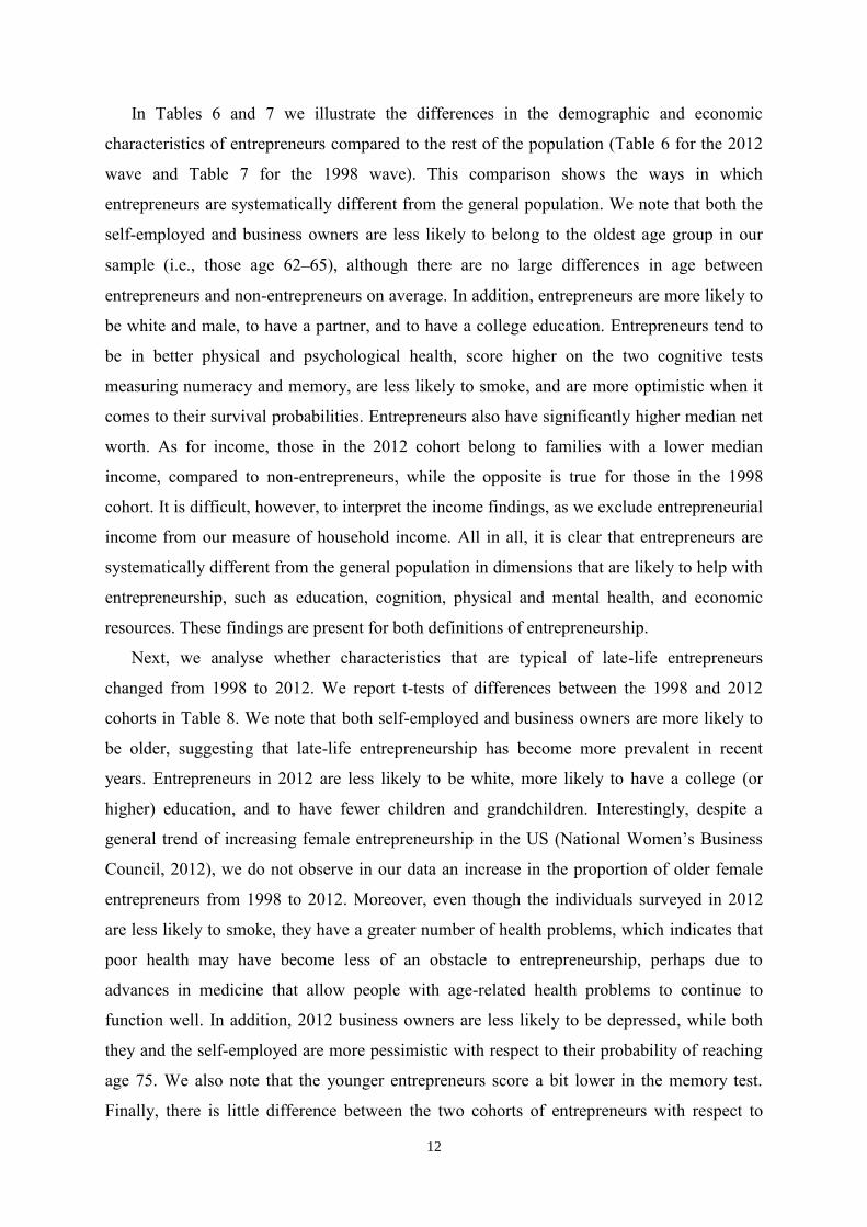
In Tables 6 and 7 we illustrate the differences in the demographic and economic
characteristics of entrepreneurs compared to the rest of the population (Table 6 for the 2012
wave and Table 7 for the 1998 wave). This comparison shows the ways in which
entrepreneurs are systematically different from the general population. We note that both the
self-employed and business owners are less likely to belong to the oldest age group in our
sample (i.e., those age 62–65), although there are no large differences in age between
entrepreneurs and non-entrepreneurs on average. In addition, entrepreneurs are more likely to
be white and male, to have a partner, and to have a college education. Entrepreneurs tend to
be in better physical and psychological health, score higher on the two cognitive tests
measuring numeracy and memory, are less likely to smoke, and are more optimistic when it
comes to their survival probabilities. Entrepreneurs also have significantly higher median net
worth. As for income, those in the 2012 cohort belong to families with a lower median
income, compared to non-entrepreneurs, while the opposite is true for those in the 1998
cohort. It is difficult, however, to interpret the income findings, as we exclude entrepreneurial
income from our measure of household income. All in all, it is clear that entrepreneurs are
systematically different from the general population in dimensions that are likely to help with
entrepreneurship, such as education, cognition, physical and mental health, and economic
resources. These findings are present for both definitions of entrepreneurship.
Next, we analyse whether characteristics that are typical of late-life entrepreneurs
changed from 1998 to 2012. We report t-tests of differences between the 1998 and 2012
cohorts in Table 8. We note that both self-employed and business owners are more likely to
be older, suggesting that late-life entrepreneurship has become more prevalent in recent
years. Entrepreneurs in 2012 are less likely to be white, more likely to have a college (or
higher) education, and to have fewer children and grandchildren. Interestingly, despite a
general trend of increasing female entrepreneurship in the US (National Women’s Business
Council, 2012), we do not observe in our data an increase in the proportion of older female
entrepreneurs from 1998 to 2012. Moreover, even though the individuals surveyed in 2012
are less likely to smoke, they have a greater number of health problems, which indicates that
poor health may have become less of an obstacle to entrepreneurship, perhaps due to
advances in medicine that allow people with age-related health problems to continue to
function well. In addition, 2012 business owners are less likely to be depressed, while both
they and the self-employed are more pessimistic with respect to their probability of reaching
age 75. We also note that the younger entrepreneurs score a bit lower in the memory test.
Finally, there is little difference between the two cohorts of entrepreneurs with respect to
13
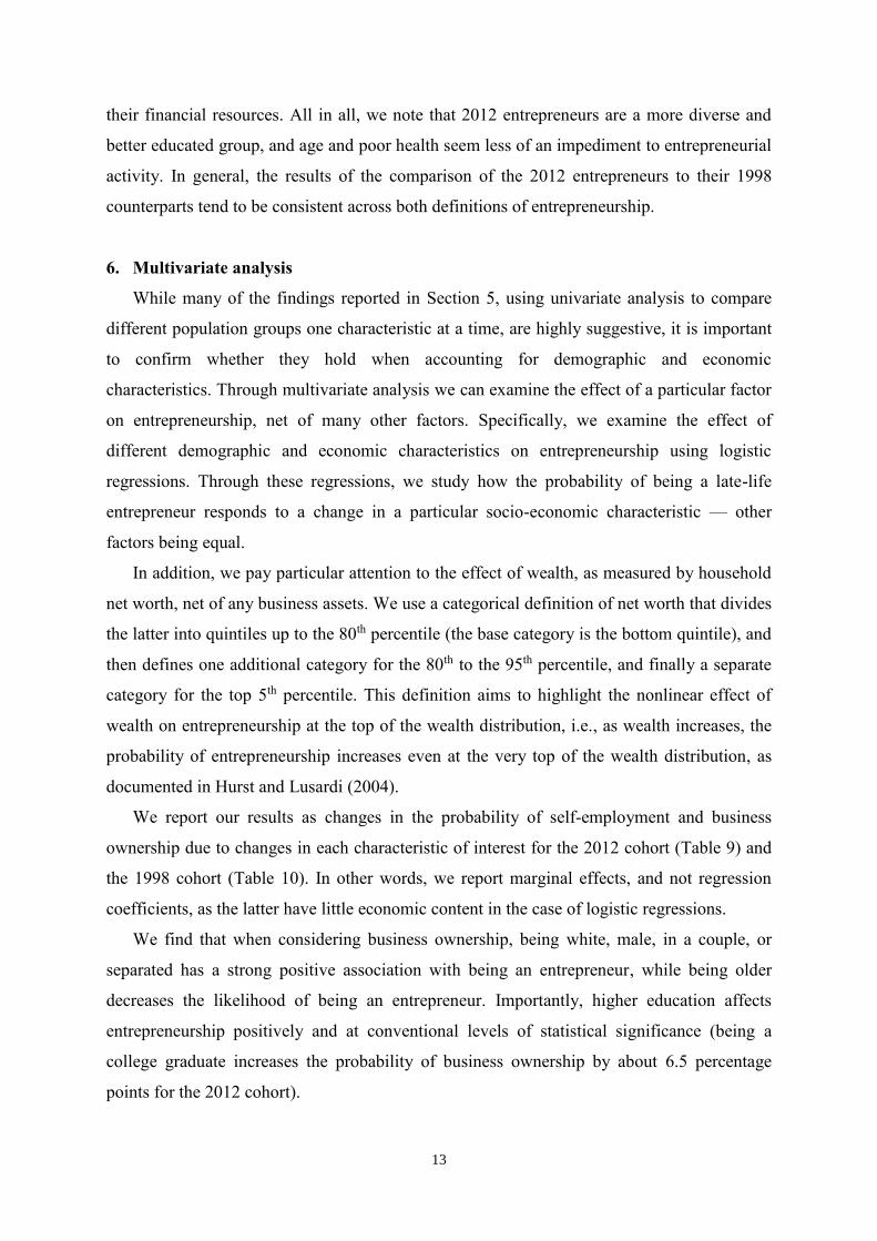
their financial resources. All in all, we note that 2012 entrepreneurs are a more diverse and
better educated group, and age and poor health seem less of an impediment to entrepreneurial
activity. In general, the results of the comparison of the 2012 entrepreneurs to their 1998
counterparts tend to be consistent across both definitions of entrepreneurship.
6. Multivariate analysis
While many of the findings reported in Section 5, using univariate analysis to compare
different population groups one characteristic at a time, are highly suggestive, it is important
to confirm whether they hold when accounting for demographic and economic
characteristics. Through multivariate analysis we can examine the effect of a particular factor
on entrepreneurship, net of many other factors. Specifically, we examine the effect of
different demographic and economic characteristics on entrepreneurship using logistic
regressions. Through these regressions, we study how the probability of being a late-life
entrepreneur responds to a change in a particular socio-economic characteristic — other
factors being equal.
In addition, we pay particular attention to the effect of wealth, as measured by household
net worth, net of any business assets. We use a categorical definition of net worth that divides
the latter into quintiles up to the 80th percentile (the base category is the bottom quintile), and
then defines one additional category for the 80th to the 95th percentile, and finally a separate
category for the top 5th percentile. This definition aims to highlight the nonlinear effect of
wealth on entrepreneurship at the top of the wealth distribution, i.e., as wealth increases, the
probability of entrepreneurship increases even at the very top of the wealth distribution, as
documented in Hurst and Lusardi (2004).
We report our results as changes in the probability of self-employment and business
ownership due to changes in each characteristic of interest for the 2012 cohort (Table 9) and
the 1998 cohort (Table 10). In other words, we report marginal effects, and not regression
coefficients, as the latter have little economic content in the case of logistic regressions.
We find that when considering business ownership, being white, male, in a couple, or
separated has a strong positive association with being an entrepreneur, while being older
decreases the likelihood of being an entrepreneur. Importantly, higher education affects
entrepreneurship positively and at conventional levels of statistical significance (being a
college graduate increases the probability of business ownership by about 6.5 percentage
points for the 2012 cohort).

14
Having physical health problems decreases the probability of entrepreneurship,8 and the
same is true for mental health problems (with the exception of business ownership among the
1998 cohort). The score on the memory test is also positively associated with
entrepreneurship for the 2012 group, while we find no economic or statistical association of
entrepreneurship with the number of children and grandchildren. Interestingly, optimism, as
proxied by the probability of survival up to age 75, is also positively associated with
entrepreneurship; an increase of 10 percentage points in this probability is associated with a
1.7 percentage increase in business ownership in the 2012 group.
As expected, higher household net worth has a strong positive effect on entrepreneurship,
and the effect is highly nonlinear: the probability of business ownership increases
significantly (by 1.6 percentage points for the 2012 cohort) even when wealth increases from
the 80th–95th percentile to the top 5th percentile.
Finally, we note that there is a negative association between household income and
entrepreneurship, but this is again a result of our definition of household income, which is net
of any entrepreneurial income. Hence, our results simply imply that the higher the non-
entrepreneurial income the less likely one is to be an entrepreneur.
To sum up, multivariate analysis confirms most of the findings of the univariate analysis
shown in Tables 6 and 7. Being an entrepreneur is positively affected by some characteristics
one would expect: being white and male and having a good education, better physical health,
optimism, and higher household net worth.
7. Taking into account the decision to work: a Heckman selection model
One important question to ask is what happens to the probability of being an
entrepreneur once we take into account the decision to work. Indeed, the decision to work
and the decision to become an entrepreneur can depend quite differently upon personal
characteristics or business conditions. For example, wealth can make it more likely that an
individual will leave the labor force, but once he/she decides to keep working, wealth can
make it easier to run a business.
Hence, we are interested in examining how a particular characteristic affects the
probability of entrepreneurship over and above its effect on the probability on working. This
conditional probability is interesting because it allows us to separate the effects of a given
8 See Zhang and Carr (2014) for additional evidence on the positive association between being in good health
and self-employment.
15
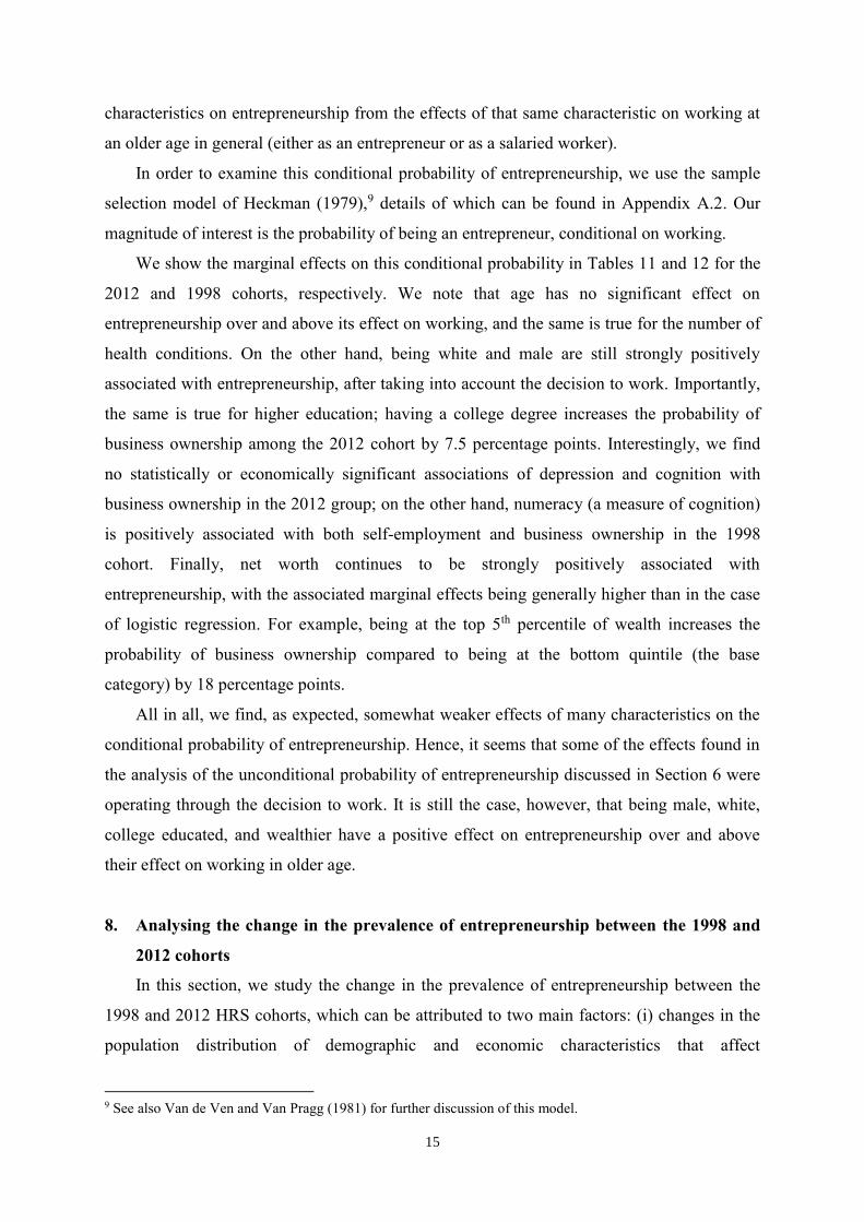
characteristics on entrepreneurship from the effects of that same characteristic on working at
an older age in general (either as an entrepreneur or as a salaried worker).
In order to examine this conditional probability of entrepreneurship, we use the sample
selection model of Heckman (1979),9 details of which can be found in Appendix A.2. Our
magnitude of interest is the probability of being an entrepreneur, conditional on working.
We show the marginal effects on this conditional probability in Tables 11 and 12 for the
2012 and 1998 cohorts, respectively. We note that age has no significant effect on
entrepreneurship over and above its effect on working, and the same is true for the number of
health conditions. On the other hand, being white and male are still strongly positively
associated with entrepreneurship, after taking into account the decision to work. Importantly,
the same is true for higher education; having a college degree increases the probability of
business ownership among the 2012 cohort by 7.5 percentage points. Interestingly, we find
no statistically or economically significant associations of depression and cognition with
business ownership in the 2012 group; on the other hand, numeracy (a measure of cognition)
is positively associated with both self-employment and business ownership in the 1998
cohort. Finally, net worth continues to be strongly positively associated with
entrepreneurship, with the associated marginal effects being generally higher than in the case
of logistic regression. For example, being at the top 5th percentile of wealth increases the
probability of business ownership compared to being at the bottom quintile (the base
category) by 18 percentage points.
All in all, we find, as expected, somewhat weaker effects of many characteristics on the
conditional probability of entrepreneurship. Hence, it seems that some of the effects found in
the analysis of the unconditional probability of entrepreneurship discussed in Section 6 were
operating through the decision to work. It is still the case, however, that being male, white,
college educated, and wealthier have a positive effect on entrepreneurship over and above
their effect on working in older age.
8. Analysing the change in the prevalence of entrepreneurship between the 1998 and
2012 cohorts
In this section, we study the change in the prevalence of entrepreneurship between the
1998 and 2012 HRS cohorts, which can be attributed to two main factors: (i) changes in the
population distribution of demographic and economic characteristics that affect
9 See also Van de Ven and Van Pragg (1981) for further discussion of this model.
16
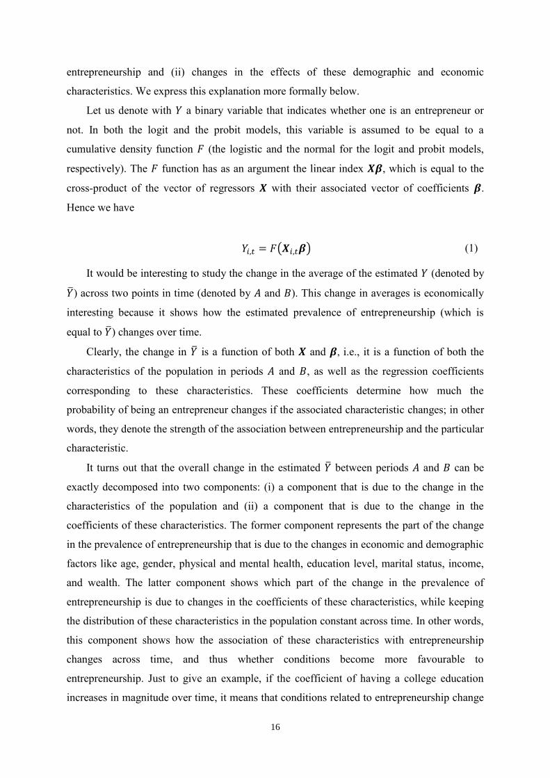
entrepreneurship and (ii) changes in the effects of these demographic and economic
characteristics. We express this explanation more formally below.
Let us denote with 𝑌 a binary variable that indicates whether one is an entrepreneur or
not. In both the logit and the probit models, this variable is assumed to be equal to a
cumulative density function 𝐹 (the logistic and the normal for the logit and probit models,
respectively). The 𝐹 function has as an argument the linear index 𝑿𝜷, which is equal to the
cross-product of the vector of regressors 𝑿 with their associated vector of coefficients 𝜷.
Hence we have
𝑌𝑖,𝑡 = 𝐹(𝑿𝑖,𝑡𝜷) (1)
It would be interesting to study the change in the average of the estimated 𝑌 (denoted by
�̅�) across two points in time (denoted by 𝐴 and 𝐵). This change in averages is economically
interesting because it shows how the estimated prevalence of entrepreneurship (which is
equal to �̅�) changes over time.
Clearly, the change in �̅� is a function of both 𝑿 and 𝜷, i.e., it is a function of both the
characteristics of the population in periods 𝐴 and 𝐵, as well as the regression coefficients
corresponding to these characteristics. These coefficients determine how much the
probability of being an entrepreneur changes if the associated characteristic changes; in other
words, they denote the strength of the association between entrepreneurship and the particular
characteristic.
It turns out that the overall change in the estimated �̅� between periods 𝐴 and 𝐵 can be
exactly decomposed into two components: (i) a component that is due to the change in the
characteristics of the population and (ii) a component that is due to the change in the
coefficients of these characteristics. The former component represents the part of the change
in the prevalence of entrepreneurship that is due to the changes in economic and demographic
factors like age, gender, physical and mental health, education level, marital status, income,
and wealth. The latter component shows which part of the change in the prevalence of
entrepreneurship is due to changes in the coefficients of these characteristics, while keeping
the distribution of these characteristics in the population constant across time. In other words,
this component shows how the association of these characteristics with entrepreneurship
changes across time, and thus whether conditions become more favourable to
entrepreneurship. Just to give an example, if the coefficient of having a college education
increases in magnitude over time, it means that conditions related to entrepreneurship change
17
across time in a way that makes a college-educated person more likely to become an
entrepreneur in the latter period than in the former.
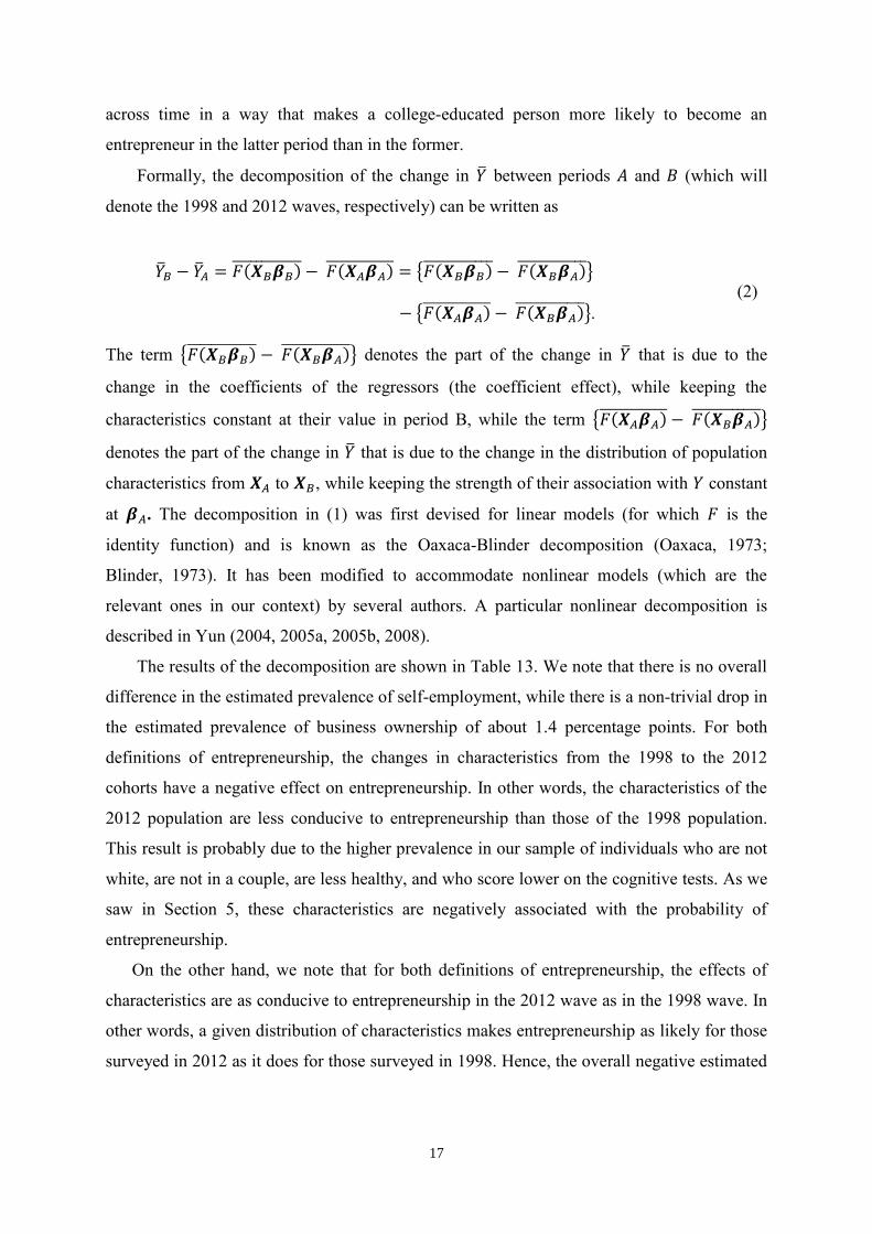
Formally, the decomposition of the change in �̅� between periods 𝐴 and 𝐵 (which will
denote the 1998 and 2012 waves, respectively) can be written as
�̅�𝐵 − �̅�𝐴 = 𝐹(𝑿𝐵𝜷𝐵)̅̅ ̅̅ ̅̅ ̅̅ ̅̅ ̅̅ − 𝐹(𝑿𝐴𝜷𝐴)̅̅ ̅̅ ̅̅ ̅̅ ̅̅ ̅̅ = {𝐹(𝑿𝐵𝜷𝐵)̅̅ ̅̅ ̅̅ ̅̅ ̅̅ ̅̅ − 𝐹(𝑿𝐵𝜷𝐴)̅̅ ̅̅ ̅̅ ̅̅ ̅̅ ̅̅ }
− {𝐹(𝑿𝐴𝜷𝐴)̅̅ ̅̅ ̅̅ ̅̅ ̅̅ ̅̅ − 𝐹(𝑿𝐵𝜷𝐴)̅̅ ̅̅ ̅̅ ̅̅ ̅̅ ̅̅ }.
(2)
The term {𝐹(𝑿𝐵𝜷𝐵)̅̅ ̅̅ ̅̅ ̅̅ ̅̅ ̅̅ − 𝐹(𝑿𝐵𝜷𝐴)̅̅ ̅̅ ̅̅ ̅̅ ̅̅ ̅̅ } denotes the part of the change in �̅� that is due to the
change in the coefficients of the regressors (the coefficient effect), while keeping the
characteristics constant at their value in period B, while the term {𝐹(𝑿𝐴𝜷𝐴)̅̅ ̅̅ ̅̅ ̅̅ ̅̅ ̅̅ − 𝐹(𝑿𝐵𝜷𝐴)̅̅ ̅̅ ̅̅ ̅̅ ̅̅ ̅̅ }
denotes the part of the change in �̅� that is due to the change in the distribution of population
characteristics from 𝑿𝐴 to 𝑿𝐵, while keeping the strength of their association with 𝑌 constant
at 𝜷𝐴. The decomposition in (1) was first devised for linear models (for which 𝐹 is the
identity function) and is known as the Oaxaca-Blinder decomposition (Oaxaca, 1973;
Blinder, 1973). It has been modified to accommodate nonlinear models (which are the
relevant ones in our context) by several authors. A particular nonlinear decomposition is
described in Yun (2004, 2005a, 2005b, 2008).
The results of the decomposition are shown in Table 13. We note that there is no overall
difference in the estimated prevalence of self-employment, while there is a non-trivial drop in
the estimated prevalence of business ownership of about 1.4 percentage points. For both
definitions of entrepreneurship, the changes in characteristics from the 1998 to the 2012
cohorts have a negative effect on entrepreneurship. In other words, the characteristics of the
2012 population are less conducive to entrepreneurship than those of the 1998 population.
This result is probably due to the higher prevalence in our sample of individuals who are not
white, are not in a couple, are less healthy, and who score lower on the cognitive tests. As we
saw in Section 5, these characteristics are negatively associated with the probability of
entrepreneurship.
On the other hand, we note that for both definitions of entrepreneurship, the effects of
characteristics are as conducive to entrepreneurship in the 2012 wave as in the 1998 wave. In
other words, a given distribution of characteristics makes entrepreneurship as likely for those
surveyed in 2012 as it does for those surveyed in 1998. Hence, the overall negative estimated
18
evolution of the business ownership rate over time is entirely due to the greater prevalence in
our sample of characteristics less favorable to entrepreneurship.
9. The causal effect of wealth on entrepreneurship
One important issue in the entrepreneurship literature is the investigation of the effect of
financial resources, and in particular wealth, on starting and maintaining a business. The
maintained hypothesis is that wealth should facilitate entrepreneurship as it is a source of
start-up funds that can alleviate liquidity constraints.10
The results from the multivariate analyses in Sections 6 and 7 point to a strong positive
association of wealth (defined as net the value of business assets) with entrepreneurship. It is
not clear, however, whether this association can be interpreted as causal, given that we are
estimating it using cross-sectional regressions. Hence, we turn to methods that can allow us to
better estimate the causal impact of wealth on entrepreneurship.
When trying to estimate the causal impact of wealth on entrepreneurship, one has to be
mindful of the possibility that unobservables that affect wealth accumulation could also affect
entrepreneurship. Such unobservables could include, e.g., competencies that enable one both
to accumulate wealth and run a business, or the propensity to take risks, which could lead
both to successful financial investment and the willingness to make a risky occupational
choice such as entrepreneurship. Hence, results from a simple regression of measures of
entrepreneurship on wealth are likely to lead to inconsistent estimates. In order to solve this
problem, one would need to use instrumental variables (IV) estimation methods; however,
instrumental variables that affect entrepreneurship but not wealth are not easy to come by,
and what has been used the literature to date has been often criticized.11
If exogenous instruments are not at hand, then one can use partial identification methods
that identify the causal effect of interest for the whole population. These methods, introduced
by Manski (1990, 1994), are nonparametric and produce bounds on the average treatment
effect (ATE henceforth). In other words, they locate the ATE in an identification region
instead of calculating a point estimate. Importantly, partial identification methods use
assumptions that are much weaker than those used in OLS and IV estimation methods.
A full discussion of the partial identification methodology can be found in Appendix
A.3. We describe here the assumptions we use to identify the average treatment effect of
wealth on entrepreneurship:
10 See the discussion of the effects of liquidity constraints on entrepreneurship in Hurst and Lusardi (2004). 11 See Hurst and Lusardi (2004).
19
1) The monotone treatment response (MTR) assumption, which states that
entrepreneurship is weakly increasing in wealth on average in our sample, i.e., not
necessarily for every individual in the sample. This is a reasonable assumption, as it
is difficult to think how higher wealth could decrease the probability of
entrepreneurship on average; after all, wealth facilitate the start of a business.
2) The monotone treatment selection (MTS) assumption, which states that those with
observed high wealth would be equally or more likely to be entrepreneurs than those
with observed lower wealth, for any given level of wealth, real or counterfactual.
This assumption is based on the fact that those with observed high wealth levels
would be expected to be more prone to entrepreneurship due to factors associated
with high wealth, such as a driven personality, family funds, and social networks
built through family and education. Importantly, the combination of the MTR and
MTS assumptions can be tested, as it implies that the observed pattern of
entrepreneurship in the sample is weakly positively correlated with wealth. This
clearly holds in our sample, as discussed in Section 5. Hence, we cannot reject the
combined MTR and MTS assumptions.
3) The monotone instrumental variables assumption (MIV). This assumption uses
variables that are weakly monotonically correlated with entrepreneurship. We choose
two different monotone instruments for entrepreneurship. First, as discussed in
Section 4, optimism is found to be positively associated with entrepreneurship in the
relevant literature. We use as a measure of optimism the probability of survival to
age 75 divided by the corresponding probability found in the US life tables, chosen
according to the age and sex of the respondent. Hence, larger values of this ratio are
more likely to denote optimism. We divide this variable in quartiles, as we need to
discretize it so as to be able to use it as a monotone instrument. The second
instrument that we use is a measure of cognition, namely the score on the delayed
recall test (recoded as a 4-level categorical variable). Entrepreneurship involves the
organization and mobilization of considerable resources so as to maintain a
prosperous business, as well as the quick perception of and reaction to changing
business conditions and opportunities. It is reasonable to assume that these tasks are
facilitated by higher cognition, and there is indeed evidence that entrepreneurs
perform better than non-entrepreneurs on cognitive tests at early ages (Levine and
Rubinstein, forthcoming). In addition, as discussed in Section 5, there is a strong
observed positive association between entrepreneurship and cognition in the HRS.
20
All in all, we believe that both our monotone instruments rest on assumptions that are
credible. They are surely much more credible than the assumption of the exogeneity
of an instrumental variable that is used in conventional estimation.
We show the results from our partial identification estimation methodology for the case
of a change in wealth from the first to the fifth quintile, i.e., the largest possible change in our
treatment variable. Due to space constraints, the remaining results for all other possible
definitions of change in wealth are available upon request from the authors.
Results are shown in Tables 14 (for 2012) and 15 (for 1998), both for self-employment
and business ownership. For each method (other than the ETS), we show the lower and upper
bounds of the treatment effect, as well as the associated lower and upper bounds of the 90%
and 95% confidence intervals.
The ETS estimate implies that the average difference in the probability of being an
entrepreneur in 2012 between those in the fifth and first wealth quintiles is about 14
percentage points and precisely estimated. The ETS treatment effect in 1998 is slightly large.
On the other hand, the ATE under NA has a predictably wide and thus uninformative
identification region, ranging from about -76 to about 82 percentage points in the case of
business ownership in 2012. This is to be expected, as making no assumptions on the data is
unlikely to lead to any useful conclusions.
Adding the MTR assumption makes the lower bound of the ATE equal to zero, while
leaving the upper bound unchanged. On the other hand, the combination of the MTS and
MTR assumptions considerably decreases the upper bound of the treatment effect, making it
equal to about 13 percentage points for the case of business ownership in 2012. The lower
bound of the treatment effect is still zero, which implies that under the MTR and MTS
assumptions, one cannot reject the hypothesis that wealth has no causal impact on
entrepreneurship.
Turning now to methods using instruments, when we combine the MTR assumption with
the use of the relative probability of survival to age 75 as a monotone instrument, the lower
bound of the ATE is still zero. The same is true when we add the MTS assumption to the
MTR and MIV assumptions, although in this case the upper bound of the treatment effect is
lowered to 11.9 percentage points for business ownership among the 2012 cohort.
When we add our second monotone instrument (i.e., delayed recall), the combination of
the MTR and MIV assumptions now results in a treatment effect that has a positive lower
bound for business ownership in the 2012 group that is equal to 1.4 percentage points and is
significant at 10%. Adding the MTS assumption to the MTR and MIV assumptions increases
21
the lower bound of the treatment effect to about 1.6 percentage points and decreases the
upper bound to about 5.2 percentage points for business ownership in the 2012 group.
It should be noted that when combining the MTR, MTS, and MIV (using two
instruments) assumptions, the bounds for some levels of expected potential outcomes cross in
a very large proportion of the bootstrap replications. This suggests that these three
assumptions have such identifying powers that the uncertainty due to the unobserved
counterfactual term in (9) is eliminated. In these cases, we estimate these potential outcomes
as a weighted average of the upper and lower bounds, as in Blundell et al. (2007).
In contrast to business ownership in the 2012 cohort, no combination of assumptions
leads to a lower bound of the treatment effect that is different from zero for self-employment
in the 2012 group. The same is true for both outcomes in the 1998 cohort, as well as for all
other possible definitions of the treatment effect of wealth (i.e., as differences between
various quantiles). This suggests that only when the treatment effect takes its maximum value
as the difference between the top and bottom wealth quantiles is there any evidence that
wealth has a causal impact on entrepreneurship. This result is consistent with the results in
Hurst and Lusardi (2004), who find that only very high levels of wealth have a positive
impact on entrepreneurship. We should also note that these results stand in contrast to the
strong associations between wealth and entrepreneurship resulting from the multivariate
analysis in Sections 7 and 8. Hence, we conclude that these results are likely to be only
associations, and driven by common factors that affect both entrepreneurship and wealth.
10. Discussion
In this paper, we have examined the characteristics of Baby Boomer entrepreneurship
using micro data from the HRS. We have compared Baby Boomer entrepreneurs to the rest of
the population, as well as to entrepreneurs in the same age group but in a different period of
time. We find that Boomer entrepreneurs are not representative of the older population; they
differ in characteristics such as ethnicity, gender, education, physical and mental health,
cognition, and economic resources. There are also changes over time, with Baby Boomer
entrepreneurs being older, more racially diverse, better educated, and in worse physical
health than the 1998 entrepreneurs.
These results point to the exceptional features that characterize entrepreneurs as well as
to the dynamic evolution of these features over time. In other words, these features are not
exclusive to a particular segment of the population, but rather can characterize more and
22
more people over time, and thus can lead to an expansion of entrepreneurship in society
provided that economic conditions are conducive to assuming entrepreneurial activities.
The fact that we find only a limited causal impact of wealth on entrepreneurship can be
interpreted as sign that business conditions are favorable enough that an entrepreneur does
not need high levels of wealth in order to start or maintain a business in older age. Reasons
for such favorable conditions could be
(i) the existence of the Internet, which allows the quick gathering and processing of
information, which is vitally important for taking advantage of business
opportunities;
(ii) medical advances, which allow people with physical limitations and health problems
to function well in a professional capacity, thus being able to meet the challenges
presented by entrepreneurial activity.
Our findings have a number of implications that are relevant to policy makers. First,
given that there is little evidence that wealth impacts entrepreneurship, credit supply to small
businesses does not seem to be a major constraint in 2012, consistent with evidence from
other studies. Hence, initiatives aimed at easing access to credit for small businesses should
be carefully examined for their impact.
Second, we find that even as recently as 2012, the share of minorities and women in
entrepreneurship is quite small. This fact points to the existence of potential significant
obstacles to entrepreneurship for these population groups, and thus policy makers could
consider measures that can lower such obstacles.
Third, it is clear from our data that business ownership among Boomers is very strongly
associated with college education. Hence, enabling access to college could help promote
entrepreneurship currently and in future years.
Fourth, to the extent that medical problems are an impediment to entrepreneurship,
policy initiatives that make health care less costly and more accessible are also likely to lead
to a larger number of entrepreneurs in the future.
23
References
Adelino, M., A. Schoar, and F. Severino (2015), “House prices, collateral, and self-
employment,” Journal of Financial Economics, 117, 288–306.
Blinder, A. S. (1973), “Wage discrimination: Reduced form and structural estimates,”
Journal of Human Resources, 8, 436–455.
Blundell, R., Gosling, A., Ichimura, H. and K. Meghir (2007), “Changes in the distribution of
male and female wages accounting for employment composition using bounds,”
Econometrica, 75, 323–363.
Bruce, D., Holtz-Eakin, D. and J. F. Quinn (2000), “Self-Employment and labor market
transitions at older ages,” Center for Retirement Research at Boston College Working
Paper 2000-13.
Cahill, K., M. Giandrea, and J. Quinn (2013), “New evidence on self-employment transitions
among older Americans with career jobs,” Bureau of Labor Statistics Working Paper
Series, WP-463.
Dawson, C. J., Meza, D., David, Henley, A. and G. R. Arabsheibani (2012),
“Entrepreneurship: cause or consequence of financial optimism?,” SSRN Scholarly
Paper No. 2157986. Available at <http://papers.ssrn.com/abstract=215798>
Evans, D. S. and B. Jovanovic (1989), “An estimated model of entrepreneurial choice under
liquidity constraints,” The Journal of Political Economy, 97, 808–827.
Fairlie, R. W. (2014), Kauffman Index of Entrepreneurial Activity.
Fraser, S. and F. J. Greene (2006), “The effects of experience on entrepreneurial optimism
and uncertainty,” Economica, 73, 169–192.
Fuchs, V. (1982), “Self-employment and labor force participation of older males,” Journal of
Human Resources, 17, 339–357.
Georgellis, Y., Sessions, J.G. and N. Tsitsianis (2005), “Windfalls, wealth and the transition
to self-employment,” Small Business Economics, 13, 407–428.
Giandrea, M. D., Cahill, K. E. and J. F. Quinn (2008), “Self-employment transitions among
older American workers with career jobs,” U.S. Bureau of Labor Statistics Working
Paper Series, WP-418.
Hauser, R. M. and R. J. Willis (2004), “Survey design and methodology in the Health and
Retirement Study and the Wisconsin Longitudinal Study,” Population and Development
Review, 30, 209–235.

24
Heckman, J. (1979), “Sample selection bias as a specification error,” Econometrica, 47, 153–
161.
Holtz-Eakin, D., Joulfaian, D. and H. S. Rosen (1994a), “Sticking it out: entrepreneurial
survival and liquidity constraints,” The Journal of Political Economy, 102, 53–75.
Holtz-Eakin, D., Joulfaian, D. and H. S. Rosen (1994b), “Entrepreneurial decisions and
liquidity constraints,” The RAND Journal of Economics, 25, 334–347.
Hurst, E. and A. Lusardi (2004), “Liquidity constraints, household wealth, and
entrepreneurship,” The Journal of Political Economy, 112, 319–47.
Imbens, G. W. and C. F. Manski (2004), “Confidence intervals for partially identified
parameters,” Econometrica, 72, 1845–57.
Karoly, L. A. and J. Zissimopoulos (2004), “Self-employment among older U.S. workers,”
Monthly Labor Review, 127, 24–47.
Kauffman Foundation (2015), “State of entrepreneurship: 2015 adddress,”
http://www.kauffman.org/~/media/kauffman_org/resources/2015/soe/2015_state_of_ent
repreneurship_address.pdf
Kreider, B. and J.V. Pepper (2007), “Disability and employment: Reevaluating the evidence
in light of reporting errors,” Journal of the American Statistical Association, 102, 432–
41.
Levine, R. and Y. Rubinstein (forthcoming), "Smart and illicit: who becomes an entrepreneur
and do they earn more?," Quarterly Journal of Economics.
Lusardi, A. (2014), “Planning and saving for retirement,” in Harper, S., and K. Hamblin
(eds), International Handbook on Ageing and Public Policy, Edward Elgar,
Northampton, MA, 2014, 474-489.
Lusardi, A. and O. Mitchell (2013), “Debt and debt management among older adults,” Global
Financial Literacy Excellence Center Working Paper 2013-2.
Manski, C. F. (1989), “Anatomy of the selection problem,” Journal of Human Resources, 24,
343–60.
Manski, C. F. (1990), “Nonparametric bounds on treatment effects,” American Economic
Review Papers and Proceedings, 80, 319–323.
Manski, C. F. (1994), “The selection problem,” in Advances in Econometrics: Sixth World
Congress, ed. by C. Sims. Cambridge, UK: Cambridge University Press, 143–170.
Manski, C. F. (1997), “Monotone treatment response,” Econometrica, 65, 1311–1334.
Manski, C. F. and J. V. Pepper (2000), “Monotone instrumental variables, with an application
to the returns to schooling,” Econometrica, 68, 997–1012.
25
Morelix, A., Russell, J., Fairlie, R.W. and E. J .Reedy (2015), “The Kauffman Index 2015:
main street entrepreneurship metropolitan area and city trends”, available at
<http://www.kauffman.org/microsites/kauffman-index/rankings/national?Report=Main
Street>
National Women’s Business Council (2012), “Women-owned businesses (WOBs): NWBC
analysis of 2012 Survey of Business Owners,”
< https://www.nwbc.gov/sites/default/files/FS_Women-Owned_Businesses.pdf>
Oaxaca, R. (1973), “Male–female wage differentials in urban labor markets,” International
Economic Review, 14, 693–709.
Özcan, B. (2011), “Only the lonely? The influence of the spouse on the transition to self-
employment,” Small Business Economics, 37, 465–492
Pagán, R. (2009), “Self-employment among people with disabilities: evidence for Europe,”
Disability and Society, 24, 217–229.
Parker, S. C. (2009), The Economics of Entrepreneurship, Cambridge: Cambridge University
Press
Puri, M. and D. T. Robinson (2013), “The economic psychology of entrepreneurship and
family business,” Journal of Economics & Management Strategy, 22, 423–444.
Van de Ven, W. P. M. M., and B. M. S. Van Pragg (1981), “The demand for deductibles in
private health insurance: A probit model with sample selection,” Journal of
Econometrics, 17, 229–252.
Wadeson, N. (2008), “Cognitive aspects of entrepreneurship: decision-making and attitudes
to risk,” in Basu, A., Casson, M., Wadeson, N. and B. Yeung (eds.) Oxford Handbook
of Entrepreneurship. Oxford: Oxford University Press.
Yun, M.-S. (2004), “Decomposing differences in the first moment,” Economics Letters, 82,
275–280.
Yun, M.-S. (2005a), “Hypothesis tests when decomposing differences in the first moment,”
Journal of Economic and Social Measurement, 30, 305–319.
Yun, M.-S. (2005b), “A simple solution to the identification problem in detailed wage de-
compositions,” Economic Inquiry, 43: 766–772. Errata 44, 198.
Yun, M.-S. (2008), “Identification problem and detailed Oaxaca decomposition: A general
solution and inference,” Journal of Economic and Social Measurement, 33, 27–38.
26
Zhang, T. and D. Carr (2014), “Does working for oneself, not others, improve older adults'
health? An investigation on health impact of self-employment,” American Journal of
Entrepreneurship, 7, 142–180.
Zissimopoulos, J. M. and L.A. Karoly (2007), “Transitions to self-employment at older ages:
The role of wealth, health, health insurance and other factors,” Labour Economics, 14,
69–295.
27
Appendix
A.1. On the definition of entrepreneurship
Given the existence in the HRS of information on business ownership only at the
household level, one could define as business owners both members of the couple (this is our
first possible definition of entrepreneurship), but this would most likely result in an over
count of entrepreneurs, as it would include partners who have little or nothing to do with the
business reported at the household-level. Such partners could, for example, be working as
salaried employees in a totally unrelated business, could have never worked in their lives, or
could be retired.
In order to deal with this issue, we construct a second category of business ownership that
excludes those who declare themselves to be fully retired, unemployed, or disabled. The
reason for this exclusion is that if respondents report any of these situations together with
business ownership, they are unlikely to be actively running a business. It most likely reflects
a passive form of ownership and thus is outside of the scope of our concept of
entrepreneurship. Hence, this exclusion removes from consideration partners in business-
owning couples who declare themselves to by professionally inactive.
Next, we exclude from business ownership those who are earning wage income, on the
grounds that their main occupation is not to run a business. This exclusion applies to all cases
of wage earners, even if both partners in a business-owning couple declare earning wage
income. However, if a self-employed person in a business-owning household reports that
his/her partner works in the family business, then the partner is still considered an
entrepreneur.12 This third possible definition of business ownership could be too restrictive,
as it could exclude entrepreneurs who draw a salary from their business, or those who might
have operate business on the side but still devoting quite a lot of their time to it.
A fourth possible definition of business ownership would be to add back to the pool of
entrepreneurs under the third definition those who belong to households that report earning
business income, even if they report earning wage income as well. It should be noted that the
earning of business income is reported at the household-level, just as business ownership.
Hence, this fourth definition might result in the over counting of business owners, as it would
include salaried employees who have no relationship with their partner’s business. On the
other hand, such salaried employees could help their partner in the operation of the business
12 This question is only asked to the self-employed, but not to those who belong to a business-owning household
without declaring themselves to be self-employed.
28
in their spare time. If so, one could argue that they should be considered entrepreneurs as
well.
Finally, a fifth possible definition of business ownership would exclude from the pool of
entrepreneurs under the fourth definition salaried partners in couples in which only one of the
two partners earns a salary. This way one could exclude from business ownership a salaried
partner who does not have anything to do with the business reported at the household level.
As can be gleaned from the above, defining entrepreneurship in the HRS is not a simple
task, and all five possible definitions can result in under- or over counting entrepreneurs in
particular circumstances. The results of our calculations as well as the entrepreneurship rate
reported in the Kauffman Index 2015 are shown in Table A.1 for those aged 55 to 64 (the
only age range for which a comparison can be made) and for the years in which the HRS and
the CPS calculations overlap, i.e. every second year from 1996 to 2014. First, we note that
the size of the HRS sample is much smaller than the CPS one (shown in columns 8 and 10,
respectively), which implies that the HRS statistics are more noisy. Be that as it may, it is
clear that the rate of self-employment (shown in column 2) as well as that of business
ownership under the first definition (simple business ownership, shown in column 3) in the
HRS are substantially larger than the rate reported in KI (shown in column 9. The same is
true for the second definition, i.e. after excluding those who are not working (column 4). On
the other hand, after excluding all those who report receiving salaried income (definition 3,
column 5), the HRS rate is substantially lower than the KI one. Putting back those who earn
business income at the household level (definition 4, column 6), brings the two indices quite
close to each other, with the possible exception of years 1998, 2000 and 2002, in which the
HRS rate is a bit lower than the KI one. Finally, excluding the single salaried partner in
business-owning couples (definition 5, column 7) brings the two rates even closer to each
other. It is also notable that both the fourth and fifth definition of business ownership exhibit
a definite downward trend of ownership over time, just as is the case with the KI rate.
Given the above results, the mainline definition of business ownership we use is the fifth
one. We use both this measure of business ownership as well as self-employment in all of our
subsequent analyses, starting with the prevalence of each form of entrepreneurship in the two
HRS waves examined and for those aged 52-65, as shown in Table 2. We clearly see that
there is no significant change in entrepreneurship in the two waves, with the prevalence of
self-employment being about 12.7% in both 1998 and 2012, and business ownership at about
between 8% and 8.5% in both 1998 and 2012. In Figures 1 and 2 we graph the prevalence of
entrepreneurship by age for the 2012 and 1998 HRS waves, respectively, and across the two

29
definitions. We note that entrepreneurship overall in the older population is in 2012 peaks at
ages 56 to 61, while it is relatively flat in 1998, with a small drop in the oldest age group, i.e.,
those age 62–65. On the other hand, the prevalence of entrepreneurship (both forms) among
workers rises with age. In other words, the older a professionally active person is, the more
likely it is that he or she will be an entrepreneur.
A.2. The Heckman selection model
The Heckman selection model consists of two equations: a probit sample selection
equation having as an outcome whether one works or not and a probit equation that models
the decision to be an entrepreneur, conditional on working. We have to do so because
working or not is a decision variable and we cannot look simply at the sample of workers
without taking into consideration the fact that it is a selected sample. Let us denote by 𝑌1 a
binary variable that indicates whether one is working or not. This variable can be thought of
as being a function of a latent continuous variable 𝑌1∗ which denotes the propensity to be
working. Let 𝑌1∗ be a function of a vector of regressors 𝒁 that has in turn an associated vector
of coefficients 𝜸. Hence, the equation for 𝑌1∗ can be written as
𝑌1,𝑖,𝑡∗ = 𝒁𝑖,𝑡𝜸 + 𝑢1,𝑖,𝑡 (A2.1)
where 𝑖 denotes the individual and 𝑡 the time period of observation, and 𝑢1 denotes a
standard normal error. We assume that 𝑌1 is equal to one if 𝑌1∗ is larger than zero, and equal
to zero otherwise, i.e.,
𝑌1,𝑖,𝑡 = 𝐼(𝑌1,𝑖,𝑡∗ > 0) (A2.2)
where I denotes the index function. Let us also assume that there is a binary variable 𝑌2 that
indicates whether one is an entrepreneur. This variable is in turn a function of a latent
continuous variable 𝑌2∗, which denotes the propensity to be an entrepreneur. Let 𝑌2
∗ be a
function of a vector of regressors 𝑿 that has, in turn, an associated vector of coefficients 𝜷.
Hence, the equation for 𝑌2∗ can be written as
𝑌2,𝑖,𝑡∗ = 𝑿𝑖,𝑡𝜷 + 𝑢2,𝑖,𝑡 (A2.3)
where 𝑢2 denotes a standard normal error. We assume that 𝑌2 is equal to one if 𝑌2∗ is larger
than zero, and equal to zero otherwise, i.e.,
30
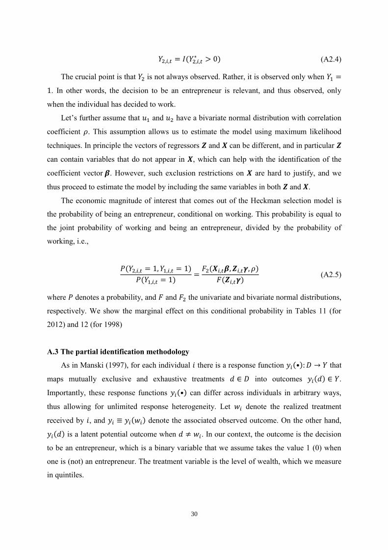
𝑌2,𝑖,𝑡 = 𝐼(𝑌2,𝑖,𝑡∗ > 0) (A2.4)
The crucial point is that 𝑌2 is not always observed. Rather, it is observed only when 𝑌1 =
1. In other words, the decision to be an entrepreneur is relevant, and thus observed, only
when the individual has decided to work.
Let’s further assume that 𝑢1 and 𝑢2 have a bivariate normal distribution with correlation
coefficient 𝜌. This assumption allows us to estimate the model using maximum likelihood
techniques. In principle the vectors of regressors 𝒁 and 𝑿 can be different, and in particular 𝒁
can contain variables that do not appear in 𝑿, which can help with the identification of the
coefficient vector 𝜷. However, such exclusion restrictions on 𝑿 are hard to justify, and we
thus proceed to estimate the model by including the same variables in both 𝒁 and 𝑿.
The economic magnitude of interest that comes out of the Heckman selection model is
the probability of being an entrepreneur, conditional on working. This probability is equal to
the joint probability of working and being an entrepreneur, divided by the probability of
working, i.e.,
𝑃(𝑌2,𝑖,𝑡 = 1, 𝑌1,𝑖,𝑡 = 1)
𝑃(𝑌1,𝑖,𝑡 = 1)=
𝐹2(𝑿𝑖,𝑡𝜷, 𝒁𝑖,𝑡𝜸, 𝜌)
𝐹(𝒁𝑖,𝑡𝜸) (A2.5)
where 𝑃 denotes a probability, and 𝐹 and 𝐹2 the univariate and bivariate normal distributions,
respectively. We show the marginal effect on this conditional probability in Tables 11 (for
2012) and 12 (for 1998)
A.3 The partial identification methodology
As in Manski (1997), for each individual 𝑖 there is a response function 𝑦𝑖(•): 𝐷 → 𝑌 that
maps mutually exclusive and exhaustive treatments 𝑑 ∈ 𝐷 into outcomes 𝑦𝑖(𝑑) ∈ 𝑌.
Importantly, these response functions 𝑦𝑖(•) can differ across individuals in arbitrary ways,
thus allowing for unlimited response heterogeneity. Let 𝑤𝑖 denote the realized treatment
received by 𝑖, and 𝑦𝑖 ≡ 𝑦𝑖(𝑤𝑖) denote the associated observed outcome. On the other hand,
𝑦𝑖(𝑑) is a latent potential outcome when 𝑑 ≠ 𝑤𝑖. In our context, the outcome is the decision
to be an entrepreneur, which is a binary variable that we assume takes the value 1 (0) when
one is (not) an entrepreneur. The treatment variable is the level of wealth, which we measure
in quintiles.
31
Let us examine for the sake of exposition two different levels of wealth, denoted by 𝑑1
and 𝑑2, respectively. Consequently, 𝑦𝑖(𝑑1) and 𝑦𝑖(𝑑2) are the two possible values of the
outcome for individual 𝑖. We would like to estimate the ATE of wealth on the decision to be
an entrepreneur, i.e.
𝐴𝑇𝐸 = 𝐸[𝑦(𝑑2)] − 𝐸[𝑦(𝑑1)] (A3.1)
Note that the ATE in (A3.1) represents the difference in two average outcomes that denote
probabilities of entrepreneurship, given that the latter is a binary variable. These average
outcomes are both evaluated using all population units while keeping all other observable and
unobservable variables fixed at their realized values (Manski 1997, p. 1322). In our context,
the ATE is equal to the difference in expected outcomes when every individual has a value of
wealth equal 𝑑2 as opposed to 𝑑1. By the law of iterated expectations, and given that
𝐸[𝑦(𝑑)|𝑤 = 𝑑] = 𝐸[𝑦|𝑤 = 𝑑], the expected outcome as a function of 𝑑 is equal to
𝐸[𝑦(𝑑)] = 𝐸[𝑦|𝑤 = 𝑑]𝑃(𝑤 = 𝑑) + 𝐸[𝑦(𝑑)|𝑤 ≠ 𝑑]𝑃(𝑤 ≠ 𝑑) (A3.2)
where 𝑃(𝑤 = 𝑑) denotes the probability that 𝑤 = 𝑑. The term 𝐸[𝑦(𝑑)|𝑤 ≠ 𝑑] in the right
hand side of (A3.2) is a counterfactual one because it denotes the expectation of the outcome
as a function of 𝑑 when the treatment actually received is different from 𝑑. On the other
hand, the remaining three terms in the right hand side of (A3.2) have sample analogues that
are observed in the data. Given that 𝐸[𝑦(𝑑)|𝑤 ≠ 𝑑] is unobserved, the unconditional
expectation 𝐸[𝑦(𝑑)] is also unobserved, i.e. it represents a potential outcome. Hence the ATE
in (A3.1) is equal to the difference between two average potential outcomes.
If one assumes that the counterfactual conditional expectation 𝐸[𝑦(𝑑)|𝑤 ≠ 𝑑] is equal to
the observed one when the treatment actually received is equal to 𝑑, i.e. if
𝐸[𝑦(𝑑)|𝑤 ≠ 𝑑] = 𝐸[𝑦|𝑤 = 𝑑] (A3.3)
then from (A3.2) it follows that
𝐸[𝑦(𝑑)] = 𝐸[𝑦|𝑤 = 𝑑] (A3.4)
Equation (A3.4) states that the unobserved potential outcome under 𝑑 is equal to the mean
outcome when the treatment actually received is equal to 𝑑. As the sample analogue of the
latter is observed in the data, one can estimate the unobserved potential outcome 𝐸[𝑦(𝑑)],
and then in turn the ATE defined in equation (A3.1), which is equal to
𝐴𝑇𝐸 = 𝐸[𝑦|𝑤 = 𝑑2] − 𝐸[𝑦|𝑤 = 𝑑1] (A3.5)

32
We refer to the estimate of the ATE in (A3.5) as the one under exogenous treatment selection
(ETS henceforth) because it is derived under the assumption that (A3.3) holds, which in turn
implies that individuals receiving different treatments (i.e. having different levels of wealth)
are not systematically different from each another. In other words, (A3.3) implies that
selection into treatment is exogenous.
Equation (A3.3) is likely to be true in the case of a randomized control trial, in which
treatment assignment is indeed exogenous. In observational data, however, (A3.3) might not
hold because treatment assignment is not random, especially when the treatment variable
reflects economic decisions taken by individuals, as is the case with wealth in our context.
Such decisions are unlikely to incur randomly, and thus there is no random assignment of the
treatment variable. Hence, the expected potential outcome 𝐸[𝑦(𝑑)] will most likely differ, for
all 𝑑, between individuals actually experiencing different levels of the treatment. In other
words, the fact that equation (A3.3) is unlikely to hold in our context is due to the
endogeneity of wealth. As already discussed, such endogeneity can be due to several factors,
which eventually all lead to non-random treatment assignment, i.e. to the violation of (A3.3).
Once one rules out the application of (A3.3), the problem of estimating the unobservable
potential outcome 𝐸[𝑦(𝑑)] arises. As a solution, Manski (1989) suggested bounding this
outcome from above and below. Let us denote the lower and upper bounds on 𝐸[𝑦(𝑑)],
computed using a particular method M, as 𝐿𝐵𝑀[𝑑] and 𝑈𝐵𝑀[𝑑], respectively.13 Given that
𝐿𝐵𝑀[𝑑] ≤ 𝐸[𝑦(𝑑)] ≤ 𝑈𝐵𝑀[𝑑], Manski (1990) points out that equation (A3.2) in turn
implies that one can bound the ATE using method M as follows:
𝐿𝐵𝑀[1] − 𝑈𝐵𝑀[0] ≤ 𝐴𝑇𝐸 ≤ 𝑈𝐵𝑀[1] − 𝐿𝐵𝑀[0] (A3.6)
The interval between the lower and the upper bound on the ATE is its identification region,
and since it is an interval the ATE is partly identified.
When calculating the upper and lower bounds on 𝐸[𝑦(𝑑)], a natural starting point is to
assume that, for any value 𝑑 of the treatment, the outcome space 𝑌 is bounded below and
above by finite values 𝑌𝑚𝑖𝑛 and 𝑌𝑚𝑎𝑥, respectively. In our application, since our outcome is a
0-1 variable denoting being an entrepreneur or not, 𝑌𝑚𝑖𝑛 = 0 and 𝑌𝑚𝑎𝑥 = 1.
As in Manski (1990), by using equation (A3.2) and after replacing the unobserved term
𝐸[𝑦(𝑑)|𝑤 ≠ 𝑑] by 𝑌𝑚𝑖𝑛 and 𝑌𝑚𝑎𝑥, one can bound 𝐸[𝑦(𝑑)] from below and above as follows:
13 It is important to note that one calculates the bounds of the potential outcome 𝐸[𝑦(𝑑)] for each value 𝑑 of the
treatment independently from all other treatment values.
33
𝐸[𝑦|𝑤 = 𝑑]𝑃(𝑤 = 𝑑) + 𝑌𝑚𝑖𝑛 𝑃(𝑤 ≠ 𝑑) =
𝐸[𝑦|𝑤 = 𝑑]𝑃(𝑤 = 𝑑)
≤ 𝐸[𝑦(𝑑)] ≤
𝐸[𝑦|𝑤 = 𝑑]𝑃(𝑤 = 𝑑) + 𝑌𝑚𝑎𝑥𝑃(𝑤 ≠ 𝑑) =
𝐸[𝑦|𝑤 = 𝑑]𝑃(𝑤 = 𝑑) + 𝑃(𝑤 ≠ 𝑑)
(A3.7)
The bounds in (A3.7) are obtained without imposing any assumptions on the data, other than
the existence of finite 𝑌𝑚𝑖𝑛 and 𝑌𝑚𝑎𝑥. We thus denote them as the no assumptions (NA)
bounds. Moreover, the NA bounds can be readily calculated using their sample analogues, as
these are observed in the data. As Manski (1989) points out, taking sample averages leads to
consistent estimates of 𝐸[𝑦|𝑤 = 𝑑], 𝑃(𝑤 = 𝑑) and 𝑃(𝑤 ≠ 𝑑).
It follows from (A3.7) that the distance between the NA upper and lower bound of
𝐸[𝑦(𝑑)] (i.e. the length of its identification interval) is equal to (𝑌𝑚𝑎𝑥 − 𝑌𝑚𝑖𝑛)𝑃(𝑤 ≠ 𝑑) =
𝑃(𝑤 ≠ 𝑑). Moreover, the distance between the upper and the lower bound of ATE computed
using the NA method is equal to 𝑌𝑚𝑎𝑥 − 𝑌𝑚𝑖𝑛 = 1 (Manski, 1990).
The NA identification region for the ATE is typically very wide, and always includes
zero. Hence, one has to make additional assumptions in order to make it narrower. The first
such assumption is that of monotone treatment response (MTR henceforth; see Manski,
1997). The MTR assumption states that for all sample units 𝑖, and for any two treatment
values 𝑑1 ∈ 𝐷 and 𝑑2 ∈ 𝐷 such that 𝑑2 > 𝑑1,
𝑦𝑖(𝑑2) ≥ 𝑦𝑖(𝑑1) (A3.8)
In our context, the MTR assumption implies that, for all individuals in our sample, having a
higher level of wealth does not decrease the propensity to be an entrepreneur. Importantly,
(A3.8) holds irrespective of the treatment actually received. Given that at each point in time
one observes only one outcome for each individual in the sample, one cannot test for the
validity of (A3.8) in isolation using the data at hand. However, the MTR assumption is a
weak inequality, i.e. it fully allows for the possibility that there is no effect of wealth on the
decision to be an entrepreneur.
In practice, we use a weaker, and thus more conservative, version of the MTR
assumption than the one in (A3.8). This weaker version states that for any treatment value
𝑑 ∈ 𝐷, and any two values 𝑑1 ∈ 𝐷 and 𝑑2 ∈ 𝐷 such that 𝑑2 > 𝑑1,
𝐸[𝑦(𝑑2)|𝑤 = 𝑑] ≥ 𝐸[𝑦(𝑑1)|𝑤 = 𝑑] (A3.9)
34
Equation (A3.9) implies that a higher level of wealth has a weakly positive effect on the
probability to be an entrepreneur, but not necessarily for every individual in the sample.
Furthermore, this average weak monotonicity holds for all subsamples that are defined by the
treatment actually received.14 Clearly, (A3.8) implies (A3.9), but the converse is not
necessarily true. The assumption that higher wealth is unlikely to reduce the probability to
become an entrepreneur is a reasonable one, as financial resources are likely to facilitate
entrepreneurship by alleviating liquidity constraints. Hence, we believe that the MTR
assumption is likely to hold in our context.
As Manski (1997) shows, the MTR assumption implies that the bounds on 𝐸[𝑦(𝑑)] can
be expressed as follows:
𝐸[𝑦|𝑤 < 𝑑]𝑃(𝑤 < 𝑑) + 𝐸[𝑦|𝑤 = 𝑑]𝑃(𝑤 = 𝑑) + 𝑌𝑚𝑖𝑛 𝑃(𝑤 > 𝑑) =
𝐸[𝑦|𝑤 < 𝑑]𝑃(𝑤 < 𝑑) + 𝐸[𝑦|𝑤 = 𝑑]𝑃(𝑤 = 𝑑)
≤ 𝐸[𝑦(𝑑)] ≤
𝑌𝑚𝑎𝑥𝑃(𝑤 < 𝑑) + 𝐸[𝑦|𝑤 = 𝑑]𝑃(𝑤 = 𝑑) + 𝐸[𝑦|𝑤 > 𝑑]𝑃(𝑤 > 𝑑) =
𝑃(𝑤 < 𝑑) + 𝐸[𝑦|𝑤 = 𝑑]𝑃(𝑤 = 𝑑) + 𝐸[𝑦|𝑤 > 𝑑]𝑃(𝑤 > 𝑑)
(A3.10)
The narrower identification region of 𝐸[𝑦(𝑑)] under MTR yields in turn a narrower
identification region of ATE resulting from (A3.10), which is now bounded below by zero
(Manski, 1997). This is to be expected, as the MTR assumption in (A3.9) rules out the
possibility that a higher level of the treatment induces a lower mean outcome, while allowing
for the possibility of a zero effect.
One can further narrow down the identification regions of 𝐸[𝑦(𝑑)] and by adding
another assumption to the MTR one, namely that of monotone treatment selection (MTS
henceforth), introduced by Manski and Pepper (2000, MP henceforth). The MTS assumption
states that for any treatment value 𝑑 ∈ 𝐷, and any two values 𝑑1 ∈ 𝐷 and 𝑑2 ∈ 𝐷 such that
𝑑2 > 𝑑1,
𝐸[𝑦(𝑑)|𝑤 = 𝑑2] ≥ 𝐸[𝑦(𝑑)|𝑤 = 𝑑1] (A3.11)
In our context, this assumption implies that those who are observed in the data to be
wealthier, are, on average and under any circumstances as defined by the actual level of
wealth, more likely to be entrepreneurs. This assumption could be justified, for example, if
being wealthier is due personality traits such as higher intelligence or a very driven
14 Given that (A3.9) holds for all values 𝑑 of the observed treatment 𝑤, it is clearly the case that the weak
monotonicity in (A3.9) applies also to the unconditional expectation, i.e. (A3.9) implies that 𝐸[𝑦(𝑑2)] ≥𝐸[𝑦(𝑑1)]. However, the converse need not be true.
35
personality. These characteristics could be associated with being an entrepreneur, and they
would manifest themselves even in the counterfactual situation in which those individuals
would have a lower level of wealth.
Another way to think about the MTS assumption is as a particular form of non-random
selection into treatment, i.e. a particular form of violation of (A3.3). If (A3.3) does not hold,
then those who choose different levels of the treatment are also systematically different with
respect to the outcome in general. The MTS assumption pins down the direction of this
difference, as it states that higher treatment levels lead to weakly higher expected outcomes.
One can test the joint validity of the MTR and MTS hypotheses using a result from
MP,15 namely that these two hypotheses jointly imply that for any two treatment values 𝑑1 ∈
𝐷 and 𝑑2 ∈ 𝐷 such that 𝑑2 > 𝑑1,
𝐸[𝑦|𝑤 = 𝑑2] ≥ 𝐸[𝑦|𝑤 = 𝑑1] (A3.12)
Equation (A3.12) states that the MTR and MTS assumptions jointly imply that the observed
mean outcomes are weakly increasing in the value of the treatment. In our data this is clearly
the case because entrepreneurship is associated with higher levels of wealth, as discussed in
Section 5. Hence, we cannot refute the validity of the joint MTR+MTS assumption.
As shown by MP, the MTR+MTS assumption implies that 𝐸[𝑦(𝑑)] can now be bounded
as follows:
𝐸[𝑦|𝑤 < 𝑑]𝑃(𝑤 < 𝑑) + 𝐸[𝑦|𝑤 = 𝑑]𝑃(𝑤 ≥ 𝑑)
≤ 𝐸[𝑦(𝑑)] ≤
𝐸[𝑦|𝑤 = 𝑑]𝑃(𝑤 ≤ 𝑑) + 𝐸[𝑦|𝑤 > 𝑑]𝑃(𝑤 > 𝑑)
(A3.13)
We note that the term 𝑌𝑚𝑖𝑛 𝑃(𝑤 > 𝑑) in the MTR lower bound in (A3.10) has now been
replaced by 𝐸[𝑦|𝑤 = 𝑑]𝑃(𝑤 > 𝑑), which can be estimated from the data. Correspondingly,
the term 𝑌𝑚𝑎𝑥 𝑃(𝑤 < 𝑑) in the MTR upper bound in (A3.10) has been replaced by 𝐸[𝑦|𝑤 =
𝑑]𝑃(𝑤 < 𝑑), which can also be estimated. As a result, the identification region of 𝐸[𝑦(𝑑)]
becomes again narrower. As MP show, the identification region of the ATE under
MTR+MTS, while narrower than the one under MTR, still has a lower bound equal to zero.
In addition to the MTR and MTS assumptions, we use the assumption of a monotone
instrumental variable (MIV henceforth), introduced by Manski and Pepper (2000), which
satisfies the following requirement for any pair of values 𝑧1, 𝑧2 of 𝑍 such that 𝑧2 > 𝑧1,
𝐸[𝑦(𝑑)|𝑍 = 𝑧2] ≥ 𝐸[𝑦(𝑑)|𝑍 = 𝑧1] (A3.14)
15 Their derivation can be found in p.1004 of MP.
36
Equation (A3.14) states that the MIV can influence the outcome in a given direction, while
the possibility of no influence whatsoever is also allowed for. Hence, the assumption of a
monotone instrumental variable is a much weaker than the assumption of an exogenous one.
It is important to note that (A3.14) captures only a positive association of 𝑍 with 𝑌; a causal
relationship is neither implied nor required.
Once one adds the MIV assumption to MTR, then for a given value 𝑧 of 𝑍 one can
calculate the maximum of the MTR lower bounds over all values of 𝑍 that are smaller or
equal to 𝑧. By (A3.14), this maximum lower bound cannot be larger than 𝐸[𝑦(𝑑)|𝑍 = 𝑧].
Similarly, one can calculate the minimum MTR upper bound over all values of 𝑍 larger or
equal to 𝑧, and (A3.14) implies that this minimum cannot be smaller than 𝐸[𝑦(𝑑)|𝑍 = 𝑧].
Hence the MTR +MIV assumption implies that
max𝑧1≤𝑧
𝐿𝐵𝑀𝑇𝑅[𝑑|𝑍 = 𝑧1] ≤ 𝐸(𝑦(𝑑)|𝑍 = 𝑧) ≤ min𝑧≥𝑧2
𝑈𝐵𝑀𝑇𝑅[𝑑|𝑍 = 𝑧2] (A3.15)
Once the bounds in (A3.15) have been computed for all 𝑧, one can take their weighted
average over all 𝑧 and bound the potential outcome 𝐸(𝑌(𝑑)) as follows:
∑ 𝑃(𝑍 = 𝑧) max𝑧1≤𝑧
𝐿𝐵𝑀𝑇𝑅[𝑑|𝑍 = 𝑧1]
𝑧
≤ ∑ 𝑃(𝑍 = 𝑧)𝐸[𝑦(𝑑)|𝑍 = 𝑧]
𝑧
= 𝐸[𝑦(𝑑)] ≤
∑ 𝑃(𝑍 = 𝑧) min𝑧≥𝑧2
𝑈𝐵𝑀𝑇𝑅[𝑑|𝑍 = 𝑧2]
𝑧
(A3.16)
Hence, by integrating 𝑍 out of the conditional expectation in (13) one can obtain bounds on
𝐸[𝑦(𝑑)].
As is the case with exogenous instruments, the weak monotonicity assumption in (A3.14)
is imposed on the unobserved potential outcome 𝐸[𝑦(𝑑)]; hence, it cannot be tested using the
observed data without imposing further assumptions. Another way to describe this situation is
that we only observe 𝐸[𝑦(𝑑)|𝑤 = 𝑑, 𝑍] and not 𝐸[𝑦(𝑑)|𝑍]. On the other hand, we also note
that the weak inequality in (A3.14) accommodates the possibility that the monotone
instruments have no effects on the outcome. As discussed in Section 9, we use two monotone
instruments, the relative probability of survival up to age 75, and the score on the delayed
recall test.
In order to conduct inferences on 𝐸[𝑦(𝑑)] and the ATE we compute confidence intervals
(CIs henceforth) that cover these magnitudes with 90% and 95% probability by using 200
37
bootstrap replications, as described in Imbens and Manski (2004). Given that the MIV
bounds involve optimization operations, the bootstrapped estimates of the bounds can be
biased. Therefore, we apply the bias correction procedure suggested by Kreider and Pepper
(2007).
The features of the bounds-based estimation method presented in this Section provide
many reasons why one would consider it a valid alternative to more commonly used methods,
e.g. OLS-, logit-, IV- or panel data-based ones, when trying to estimate the causal effect of
interest. First, bounds-based estimation is completely nonparametric, as it only involves
taking simple sample averages of the outcome and the treatment. Hence, it is not affected by
the problem of estimates resulting from local minima and maxima. Second, bounds-based
estimation leads to estimates of the ATE across all sample units, and not of the LATE as is
the case with IV estimation when the treatment effect is heterogeneous across the population.
Third, it allows for arbitrary forms of heterogeneity of the treatment effect because the ATE
is just an average magnitude across sample units. Hence, the treatment effect for each sample
unit can depend on any other variable in a fully flexible way. Such unlimited heterogeneity of
the treatment effect is not typically allowed for, as in most estimation methods one makes
particular assumptions about how the treatment variable enters into the specification.
Moreover, if one is interested in studying the heterogeneity of the treatment effect in
particular dimensions in the context of partial identification, then one can simply restrict
estimation to subsamples defined by particular combinations of values of control variables.
Fourth, as already discussed, the computation of the ATE takes the distribution of all
observables and unobservables in the sample as given. Hence, one does not need to worry
about: i) which variables to add in the empirical specification; ii) the manner in which they
appear; iii) whether they are endogenous or not. Fifth, bounds-based estimation
accommodates any form of endogeneity (e.g. due to both time-varying and time-invariant
unobservables or selectivity), as it allows for non-random selection into treatment in any
form. This also implies that one does not need to assume particular properties of an error
term, as is the case with regression methods. Sixth, partial identification methods use few and
quite mild assumptions to narrow the identification region of the estimates. Importantly, they
are completely transparent about how the addition of each assumption affects the
identification region. In contrast, most commonly used estimation methods typically impose
many assumptions on the empirical model at the same time, and thus it is typically not clear
how each assumption affects estimates. Seventh, partial identification methods allow the use
of monotone IVs, which can tighten identification regions. As is the case with standard IV
38
estimation, the assumptions behind these IVs cannot be tested without making further
assumptions. However, MIVs, which cannot be used in standard IV estimation, are based on
assumptions that are much weaker than those of exogenous IVs. Finally, in bounds-based
estimation one uses the data as a cross-section, and thus panel data are not required. One can
accommodate any dependencies among sample units (e.g. due to repeated observation or
features of the sampling process) through the appropriate clustering and stratification when
bootstrapping standard errors.
On the other hand, partial identification methods can sometimes lead to identification
regions that are wide, and thus do not allow one to draw strong conclusions about the effect
of interest. This is the price that sometimes one has to pay for imposing very few and weak
assumptions on the data. As Manski (1994) notes, the point identification obtained by more
commonly used estimation methods may give one a false certainty about results, as the
reduction in uncertainty is obtained through assumptions that are not testable, and that might
not hold in the data.
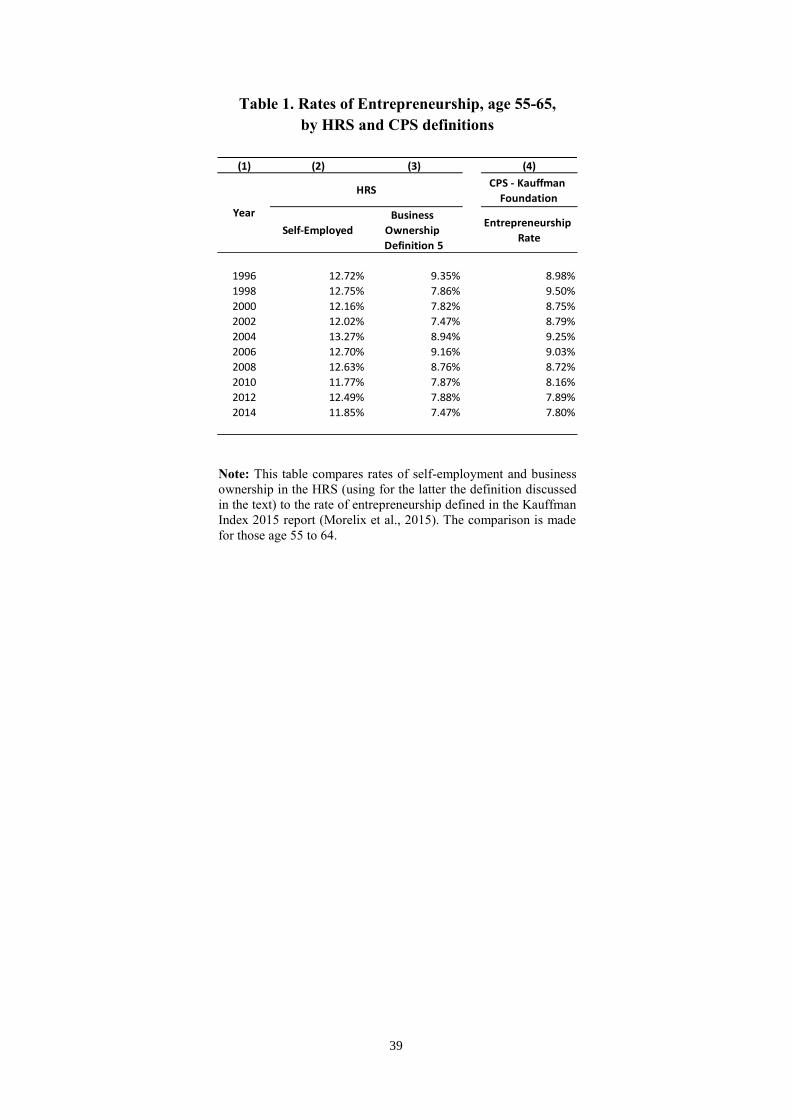
39
Table 1. Rates of Entrepreneurship, age 55-65,
by HRS and CPS definitions
(1) (2) (3) (4)
CPS - Kauffman
Foundation
Self-Employed
Business
Ownership
Definition 5
Entrepreneurship
Rate
1996 12.72% 9.35% 8.98%
1998 12.75% 7.86% 9.50%
2000 12.16% 7.82% 8.75%
2002 12.02% 7.47% 8.79%
2004 13.27% 8.94% 9.25%
2006 12.70% 9.16% 9.03%
2008 12.63% 8.76% 8.72%
2010 11.77% 7.87% 8.16%
2012 12.49% 7.88% 7.89%
2014 11.85% 7.47% 7.80%
Year
HRS
Note: This table compares rates of self-employment and business
ownership in the HRS (using for the latter the definition discussed
in the text) to the rate of entrepreneurship defined in the Kauffman
Index 2015 report (Morelix et al., 2015). The comparison is made
for those age 55 to 64.
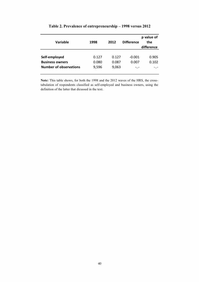
40
Table 2. Prevalence of entrepreneurship – 1998 versus 2012
Variable 1998 2012 Difference
p value of
the
difference
Self-employed 0.127 0.127 -0.001 0.905
Business owners 0.080 0.087 0.007 0.102
Number of observations 9,596 9,063 -..- -..-
Note: This table shows, for both the 1998 and the 2012 waves of the HRS, the cross-
tabulation of respondents classified as self-employed and business owners, using the
definition of the latter that dicussed in the text.
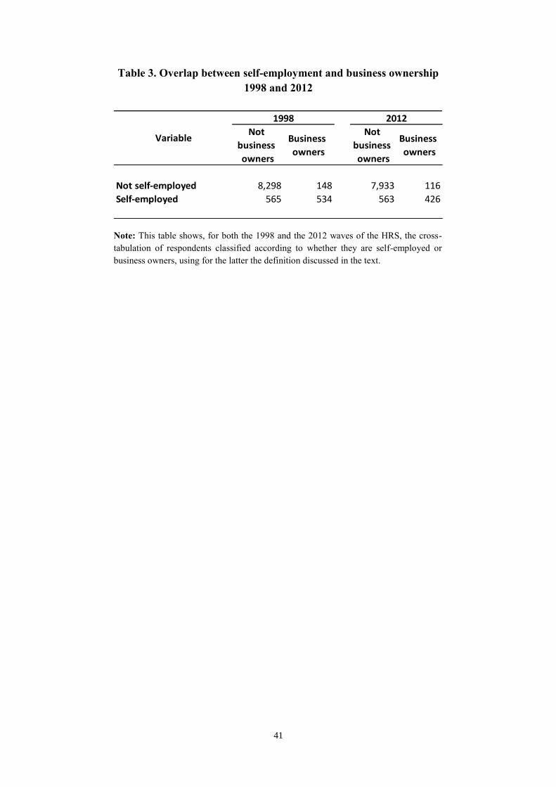
41
Table 3. Overlap between self-employment and business ownership
1998 and 2012
Not
business
owners
Business
owners
Not
business
owners
Business
owners
Not self-employed 8,298 148 7,933 116
Self-employed 565 534 563 426
Variable
1998 2012
Note: This table shows, for both the 1998 and the 2012 waves of the HRS, the cross-
tabulation of respondents classified according to whether they are self-employed or
business owners, using for the latter the definition discussed in the text.
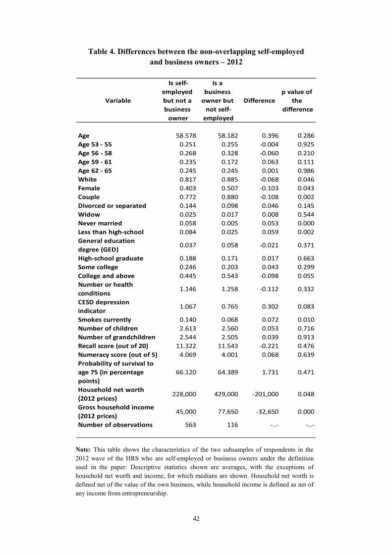
42
Table 4. Differences between the non-overlapping self-employed
and business owners – 2012
Variable
Is self-
employed
but not a
business
owner
Is a
business
owner but
not self-
employed
Difference
p value of
the
difference
Age 58.578 58.182 0.396 0.286
Age 53 - 55 0.251 0.255 -0.004 0.925
Age 56 - 58 0.268 0.328 -0.060 0.210
Age 59 - 61 0.235 0.172 0.063 0.111
Age 62 - 65 0.245 0.245 0.001 0.986
White 0.817 0.885 -0.068 0.046
Female 0.403 0.507 -0.103 0.043
Couple 0.772 0.880 -0.108 0.002
Divorced or separated 0.144 0.098 0.046 0.145
Widow 0.025 0.017 0.008 0.544
Never married 0.058 0.005 0.053 0.000
Less than high-school 0.084 0.025 0.059 0.002
General education
degree (GED)0.037 0.058 -0.021 0.371
High-school graduate 0.188 0.171 0.017 0.663
Some college 0.246 0.203 0.043 0.299
College and above 0.445 0.543 -0.098 0.055
Number or health
conditions1.146 1.258 -0.112 0.332
CESD depression
indicator1.067 0.765 0.302 0.083
Smokes currently 0.140 0.068 0.072 0.010
Number of children 2.613 2.560 0.053 0.716
Number of grandchildren 2.544 2.505 0.039 0.913
Recall score (out of 20) 11.322 11.543 -0.221 0.476
Numeracy score (out of 5) 4.069 4.001 0.068 0.639
Probability of survival to
age 75 (in percentage
points)
66.120 64.389 1.731 0.471
Household net worth
(2012 prices)228,000 429,000 -201,000 0.048
Gross household income
(2012 prices)45,000 77,650 -32,650 0.000
Number of observations 563 116 -..- -..-
Note: This table shows the characteristics of the two subsamples of respondents in the
2012 wave of the HRS who are self-employed or business owners under the definition
used in the paper. Descriptive statistics shown are averages, with the exceptions of
household net worth and income, for which medians are shown. Household net worth is
defined net of the value of the own business, while household income is defined as net of
any income from entrepreneurship.
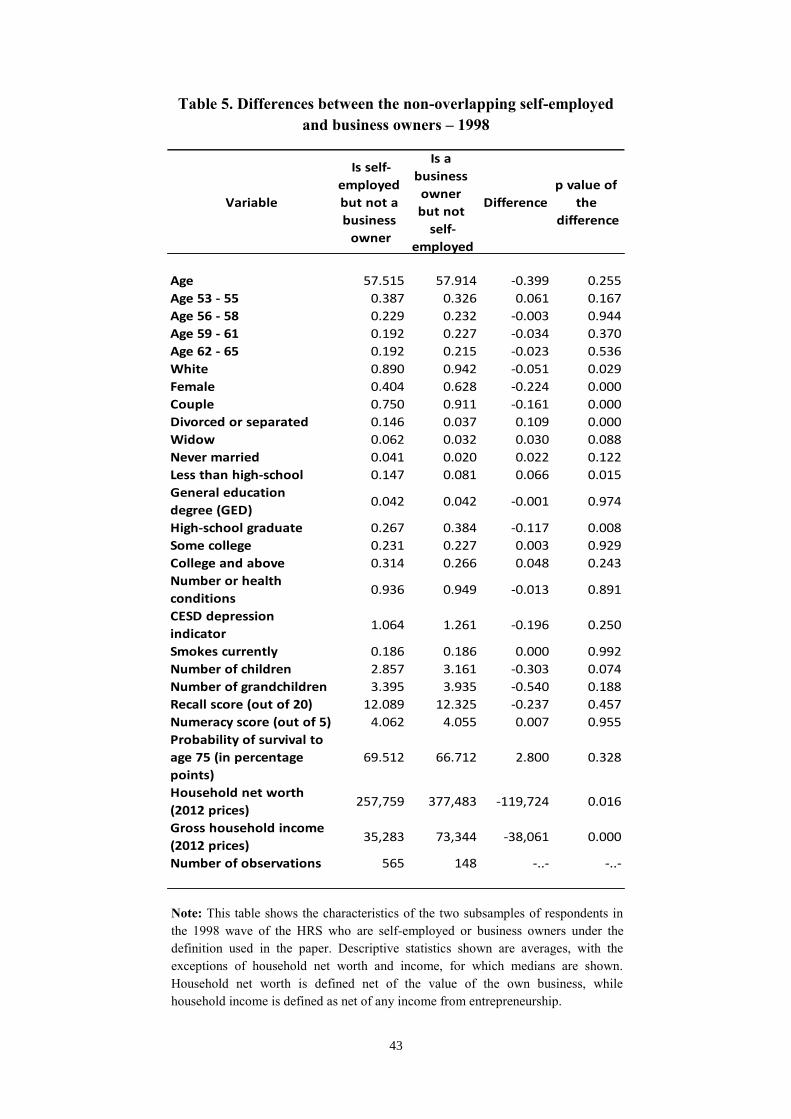
43
Table 5. Differences between the non-overlapping self-employed
and business owners – 1998
Variable
Is self-
employed
but not a
business
owner
Is a
business
owner
but not
self-
employed
Difference
p value of
the
difference
Age 57.515 57.914 -0.399 0.255
Age 53 - 55 0.387 0.326 0.061 0.167
Age 56 - 58 0.229 0.232 -0.003 0.944
Age 59 - 61 0.192 0.227 -0.034 0.370
Age 62 - 65 0.192 0.215 -0.023 0.536
White 0.890 0.942 -0.051 0.029
Female 0.404 0.628 -0.224 0.000
Couple 0.750 0.911 -0.161 0.000
Divorced or separated 0.146 0.037 0.109 0.000
Widow 0.062 0.032 0.030 0.088
Never married 0.041 0.020 0.022 0.122
Less than high-school 0.147 0.081 0.066 0.015
General education
degree (GED)0.042 0.042 -0.001 0.974
High-school graduate 0.267 0.384 -0.117 0.008
Some college 0.231 0.227 0.003 0.929
College and above 0.314 0.266 0.048 0.243
Number or health
conditions0.936 0.949 -0.013 0.891
CESD depression
indicator1.064 1.261 -0.196 0.250
Smokes currently 0.186 0.186 0.000 0.992
Number of children 2.857 3.161 -0.303 0.074
Number of grandchildren 3.395 3.935 -0.540 0.188
Recall score (out of 20) 12.089 12.325 -0.237 0.457
Numeracy score (out of 5) 4.062 4.055 0.007 0.955
Probability of survival to
age 75 (in percentage
points)
69.512 66.712 2.800 0.328
Household net worth
(2012 prices)257,759 377,483 -119,724 0.016
Gross household income
(2012 prices)35,283 73,344 -38,061 0.000
Number of observations 565 148 -..- -..-
Note: This table shows the characteristics of the two subsamples of respondents in
the 1998 wave of the HRS who are self-employed or business owners under the
definition used in the paper. Descriptive statistics shown are averages, with the
exceptions of household net worth and income, for which medians are shown.
Household net worth is defined net of the value of the own business, while
household income is defined as net of any income from entrepreneurship.
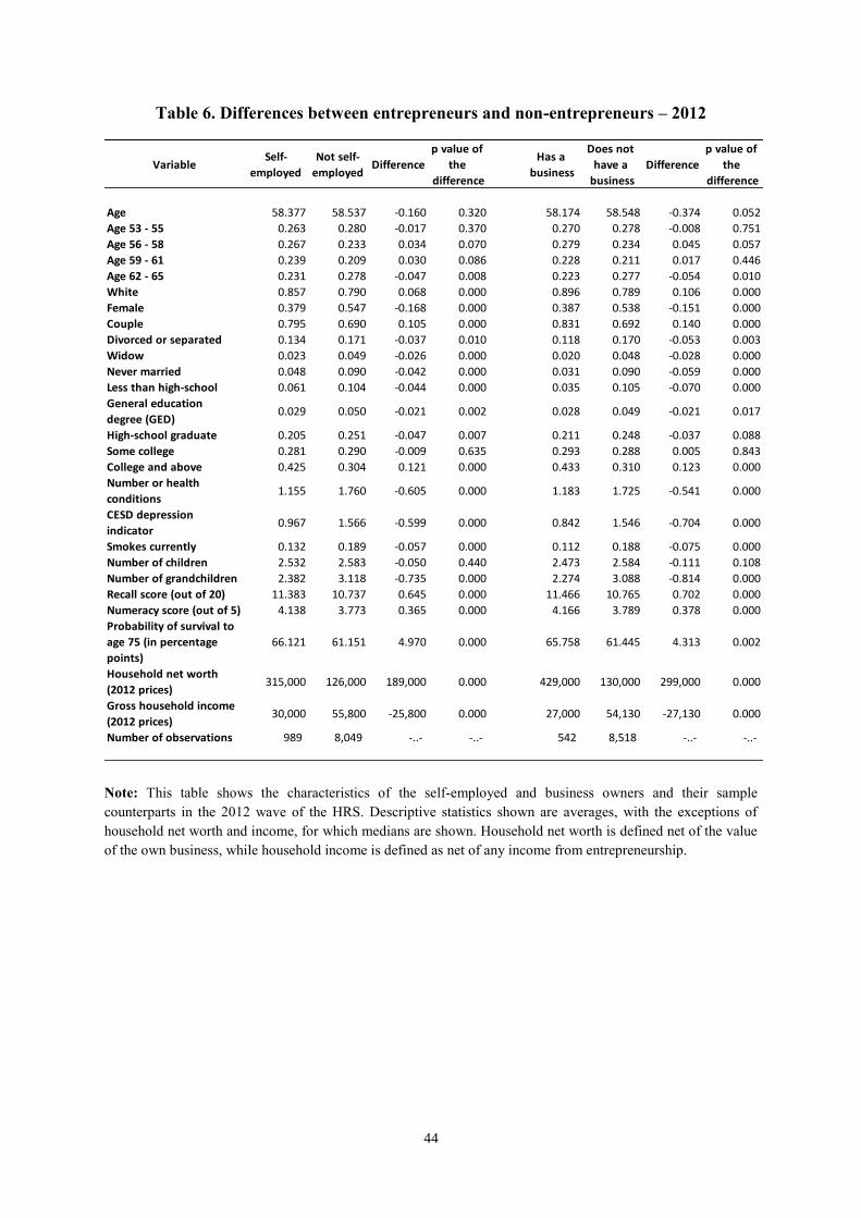
44
Table 6. Differences between entrepreneurs and non-entrepreneurs – 2012
VariableSelf-
employed
Not self-
employedDifference
p value of
the
difference
Has a
business
Does not
have a
business
Difference
p value of
the
difference
Age 58.377 58.537 -0.160 0.320 . 58.174 58.548 -0.374 0.052
Age 53 - 55 0.263 0.280 -0.017 0.370 . 0.270 0.278 -0.008 0.751
Age 56 - 58 0.267 0.233 0.034 0.070 . 0.279 0.234 0.045 0.057
Age 59 - 61 0.239 0.209 0.030 0.086 . 0.228 0.211 0.017 0.446
Age 62 - 65 0.231 0.278 -0.047 0.008 . 0.223 0.277 -0.054 0.010
White 0.857 0.790 0.068 0.000 . 0.896 0.789 0.106 0.000
Female 0.379 0.547 -0.168 0.000 . 0.387 0.538 -0.151 0.000
Couple 0.795 0.690 0.105 0.000 . 0.831 0.692 0.140 0.000
Divorced or separated 0.134 0.171 -0.037 0.010 . 0.118 0.170 -0.053 0.003
Widow 0.023 0.049 -0.026 0.000 . 0.020 0.048 -0.028 0.000
Never married 0.048 0.090 -0.042 0.000 0.031 0.090 -0.059 0.000
Less than high-school 0.061 0.104 -0.044 0.000 . 0.035 0.105 -0.070 0.000
General education
degree (GED)0.029 0.050 -0.021 0.002 . 0.028 0.049 -0.021 0.017
High-school graduate 0.205 0.251 -0.047 0.007 . 0.211 0.248 -0.037 0.088
Some college 0.281 0.290 -0.009 0.635 . 0.293 0.288 0.005 0.843
College and above 0.425 0.304 0.121 0.000 . 0.433 0.310 0.123 0.000
Number or health
conditions1.155 1.760 -0.605 0.000 . 1.183 1.725 -0.541 0.000
CESD depression
indicator0.967 1.566 -0.599 0.000 . 0.842 1.546 -0.704 0.000
Smokes currently 0.132 0.189 -0.057 0.000 . 0.112 0.188 -0.075 0.000
Number of children 2.532 2.583 -0.050 0.440 . 2.473 2.584 -0.111 0.108
Number of grandchildren 2.382 3.118 -0.735 0.000 . 2.274 3.088 -0.814 0.000
Recall score (out of 20) 11.383 10.737 0.645 0.000 . 11.466 10.765 0.702 0.000
Numeracy score (out of 5) 4.138 3.773 0.365 0.000 . 4.166 3.789 0.378 0.000
Probability of survival to
age 75 (in percentage
points)
66.121 61.151 4.970 0.000 65.758 61.445 4.313 0.002
Household net worth
(2012 prices)315,000 126,000 189,000 0.000 . 429,000 130,000 299,000 0.000
Gross household income
(2012 prices)30,000 55,800 -25,800 0.000 . 27,000 54,130 -27,130 0.000
Number of observations 989 8,049 -..- -..- 542 8,518 -..- -..-
Note: This table shows the characteristics of the self-employed and business owners and their sample
counterparts in the 2012 wave of the HRS. Descriptive statistics shown are averages, with the exceptions of
household net worth and income, for which medians are shown. Household net worth is defined net of the value
of the own business, while household income is defined as net of any income from entrepreneurship.
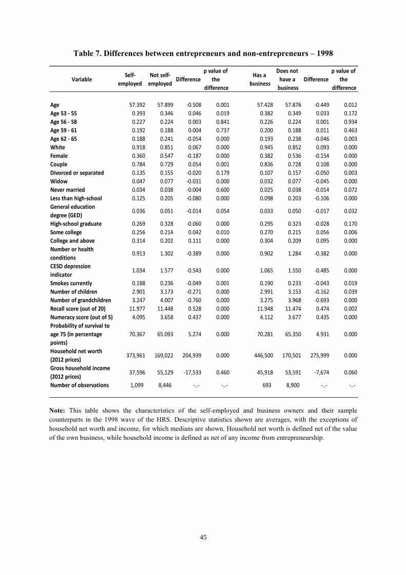
45
Table 7. Differences between entrepreneurs and non-entrepreneurs – 1998
Note: This table shows the characteristics of the self-employed and business owners and their sample
counterparts in the 1998 wave of the HRS. Descriptive statistics shown are averages, with the exceptions of
household net worth and income, for which medians are shown. Household net worth is defined net of the value
of the own business, while household income is defined as net of any income from entrepreneurship.
VariableSelf-
employed
Not self-
employedDifference
p value of
the
difference
Has a
business
Does not
have a
business
Difference
p value of
the
difference
Age 57.392 57.899 -0.508 0.001 . 57.428 57.876 -0.449 0.012
Age 53 - 55 0.393 0.346 0.046 0.019 . 0.382 0.349 0.033 0.172
Age 56 - 58 0.227 0.224 0.003 0.841 . 0.226 0.224 0.001 0.934
Age 59 - 61 0.192 0.188 0.004 0.737 . 0.200 0.188 0.011 0.463
Age 62 - 65 0.188 0.241 -0.054 0.000 . 0.193 0.238 -0.046 0.003
White 0.918 0.851 0.067 0.000 . 0.945 0.852 0.093 0.000
Female 0.360 0.547 -0.187 0.000 . 0.382 0.536 -0.154 0.000
Couple 0.784 0.729 0.054 0.001 . 0.836 0.728 0.108 0.000
Divorced or separated 0.135 0.155 -0.020 0.179 . 0.107 0.157 -0.050 0.003
Widow 0.047 0.077 -0.031 0.000 . 0.032 0.077 -0.045 0.000
Never married 0.034 0.038 -0.004 0.600 0.025 0.038 -0.014 0.072
Less than high-school 0.125 0.205 -0.080 0.000 . 0.098 0.203 -0.106 0.000
General education
degree (GED)0.036 0.051 -0.014 0.054 . 0.033 0.050 -0.017 0.032
High-school graduate 0.269 0.328 -0.060 0.000 . 0.295 0.323 -0.028 0.170
Some college 0.256 0.214 0.042 0.010 . 0.270 0.215 0.056 0.006
College and above 0.314 0.202 0.111 0.000 . 0.304 0.209 0.095 0.000
Number or health
conditions0.913 1.302 -0.389 0.000 . 0.902 1.284 -0.382 0.000
CESD depression
indicator1.034 1.577 -0.543 0.000 . 1.065 1.550 -0.485 0.000
Smokes currently 0.188 0.236 -0.049 0.001 . 0.190 0.233 -0.043 0.019
Number of children 2.901 3.173 -0.271 0.000 . 2.991 3.153 -0.162 0.039
Number of grandchildren 3.247 4.007 -0.760 0.000 . 3.275 3.968 -0.693 0.000
Recall score (out of 20) 11.977 11.448 0.528 0.000 . 11.948 11.474 0.474 0.002
Numeracy score (out of 5) 4.095 3.658 0.437 0.000 . 4.112 3.677 0.435 0.000
Probability of survival to
age 75 (in percentage
points)
70.367 65.093 5.274 0.000 70.281 65.350 4.931 0.000
Household net worth
(2012 prices)373,961 169,022 204,939 0.000 . 446,500 170,501 275,999 0.000
Gross household income
(2012 prices)37,596 55,129 -17,533 0.460 . 45,918 53,591 -7,674 0.060
Number of observations 1,099 8,446 -..- -..- 693 8,900 -..- -..-
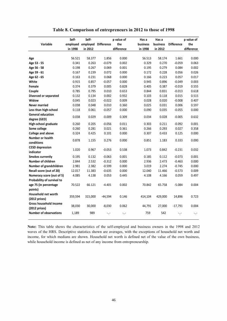
46
Table 8. Comparison of entrepreneurs in 2012 to those of 1998
Variable
Self-
employed
in 1998
Self-
employed
in 2012
Difference
p value of
the
difference
Has a
business
in 1998
Has a
business
in 2012
Difference
p value of
the
difference
Age 56.521 58.377 1.856 0.000 . 56.513 58.174 1.661 0.000
Age 53 - 55 0.341 0.263 -0.079 0.002 . 0.329 0.270 -0.059 0.063
Age 56 - 58 0.198 0.267 0.069 0.001 . 0.195 0.279 0.084 0.002
Age 59 - 61 0.167 0.239 0.072 0.000 . 0.172 0.228 0.056 0.026
Age 62 - 65 0.163 0.231 0.068 0.000 . 0.166 0.223 0.057 0.017
White 0.915 0.857 -0.057 0.000 . 0.945 0.896 -0.049 0.003
Female 0.374 0.379 0.005 0.828 . 0.405 0.387 -0.019 0.555
Couple 0.785 0.795 0.010 0.653 . 0.844 0.831 -0.013 0.618
Divorced or separated 0.132 0.134 0.002 0.932 . 0.103 0.118 0.015 0.515
Widow 0.045 0.023 -0.022 0.009 . 0.028 0.020 -0.008 0.407
Never married 0.038 0.048 0.010 0.360 0.025 0.031 0.006 0.597
Less than high-school 0.118 0.061 -0.057 0.000 . 0.090 0.035 -0.055 0.000
General education
degree (GED)0.038 0.029 -0.009 0.309 . 0.034 0.028 -0.005 0.632
High-school graduate 0.260 0.205 -0.056 0.011 . 0.303 0.211 -0.092 0.001
Some college 0.260 0.281 0.021 0.361 . 0.266 0.293 0.027 0.358
College and above 0.324 0.425 0.101 0.000 . 0.307 0.433 0.125 0.000
Number or health
conditions0.878 1.155 0.276 0.000 . 0.851 1.183 0.333 0.000
CESD depression
indicator1.020 0.967 -0.053 0.538 . 1.073 0.842 -0.231 0.032
Smokes currently 0.195 0.132 -0.063 0.001 . 0.185 0.112 -0.073 0.001
Number of children 2.844 2.532 -0.312 0.000 . 2.936 2.473 -0.463 0.000
Number of grandchildren 2.981 2.382 -0.599 0.000 . 3.019 2.274 -0.745 0.000
Recall score (out of 20) 12.017 11.383 -0.635 0.000 . 12.040 11.466 -0.573 0.009
Numeracy score (out of 5) 4.085 4.138 0.053 0.445 . 4.108 4.166 0.059 0.497
Probability of survival to
age 75 (in percentage
points)
70.522 66.121 -4.401 0.002 70.842 65.758 -5.084 0.004
Household net worth
(2012 prices)359,594 315,000 -44,594 0.146 414,104 429,000 14,896 0.723
Gross household income
(2012 prices)38,030 30,000 -8,030 0.062 44,791 27,000 -17,791 0.004
Number of observations 1,189 989 -..- -..- 759 542 -..- -..-
Note: This table shows the characteristics of the self-employed and business owners in the 1998 and 2012
waves of the HRS. Descriptive statistics shown are averages, with the exceptions of household net worth and
income, for which medians are shown. Household net worth is defined net of the value of the own business,
while household income is defined as net of any income from entrepreneurship.

47
Table 9. Logit results for entrepreneurship - 2012
Marginal
EffectStd. Error t statistic p value
Marginal
EffectStd. Error t statistic p value
Age 56 - 58 0.013 0.008 1.585 0.113 0.003 0.007 0.404 0.686
Age 59 - 61 0.012 0.009 1.352 0.176 -0.009 0.007 -1.270 0.204
Age 62 - 65 -0.015 0.010 -1.480 0.139 -0.015 0.008 -1.837 0.066
White 0.026 0.008 3.209 0.001 0.035 0.007 4.805 0.000
Female -0.057 0.007 -8.592 0.000 -0.032 0.005 -6.998 0.000
Couple 0.074 0.015 4.842 0.000 0.052 0.014 3.859 0.000
Divorced or separated 0.035 0.016 2.247 0.025 0.028 0.014 2.000 0.045
Widow 0.022 0.022 1.030 0.303 -0.008 0.021 -0.400 0.689
General education degree (GED) 0.041 0.019 2.193 0.028 0.054 0.019 2.908 0.004
High-school graduate 0.032 0.013 2.459 0.014 0.053 0.014 3.733 0.000
Some college 0.053 0.013 4.110 0.000 0.062 0.014 4.438 0.000
College and above 0.065 0.014 4.565 0.000 0.065 0.015 4.386 0.000
Number or health conditions -0.023 0.003 -8.055 0.000 -0.008 0.002 -3.979 0.000
CESD depression indicator -0.008 0.002 -3.958 0.000 -0.005 0.002 -3.142 0.002
Smokes currently -0.017 0.009 -1.944 0.052 -0.009 0.008 -1.178 0.239
Number of children 0.004 0.002 1.570 0.116 0.000 0.002 0.084 0.933
Number of grandchildren -0.001 0.001 -0.840 0.401 0.000 0.001 -0.256 0.798
Recall score (out of 20) 0.005 0.001 4.181 0.000 0.002 0.001 2.036 0.042
Numeracy score (out of 5) 0.002 0.003 0.898 0.369 0.002 0.002 0.911 0.362
Probability of survival to age 75 (in
percentage points)0.000 0.000 1.978 0.048 0.000 0.000 1.857 0.063
Household net worth - 2nd
quintile 0.026 0.010 2.638 0.008 0.033 0.010 3.323 0.001
Household net worth - 3d quintile 0.065 0.011 6.010 0.000 0.067 0.010 6.740 0.000
Household net worth - 80th
to 95th
percentile0.094 0.012 7.854 0.000 0.086 0.011 8.020 0.000
Household net worth - top 5th
percentile0.139 0.018 7.758 0.000 0.102 0.014 7.114 0.000
Gross household income - 2nd
quartile -0.114 0.010 -11.615 0.000 -0.073 0.009 -8.370 0.000
Gross household income - 3d quartile -0.154 0.009 -16.319 0.000 -0.096 0.008 -11.680 0.000
Gross household income - 4th
quartile -0.210 0.010 -20.760 0.000 -0.115 0.008 -14.463 0.000
Number of observations 7,918 7,924
Variable
Probability of being self-employed
(unconditional)
Probability of owning a business
(unconditional)
Notes: This table shows the marginal effects from a logit regression of a binary variable denoting self-
employment or business ownership on demographic and economic characteristics of the respondents in the
2012 wave of the HRS. Marginal effects represent the change in the unconditional probability of the outcome
due to a change in the regressor by one unit. The base (omitted) categories for the categorical regressors are
age 52–55, non-whites, males, those never married, those with less than high school education, non-smokers,
and households in the first quartiles of household net worth and gross income.
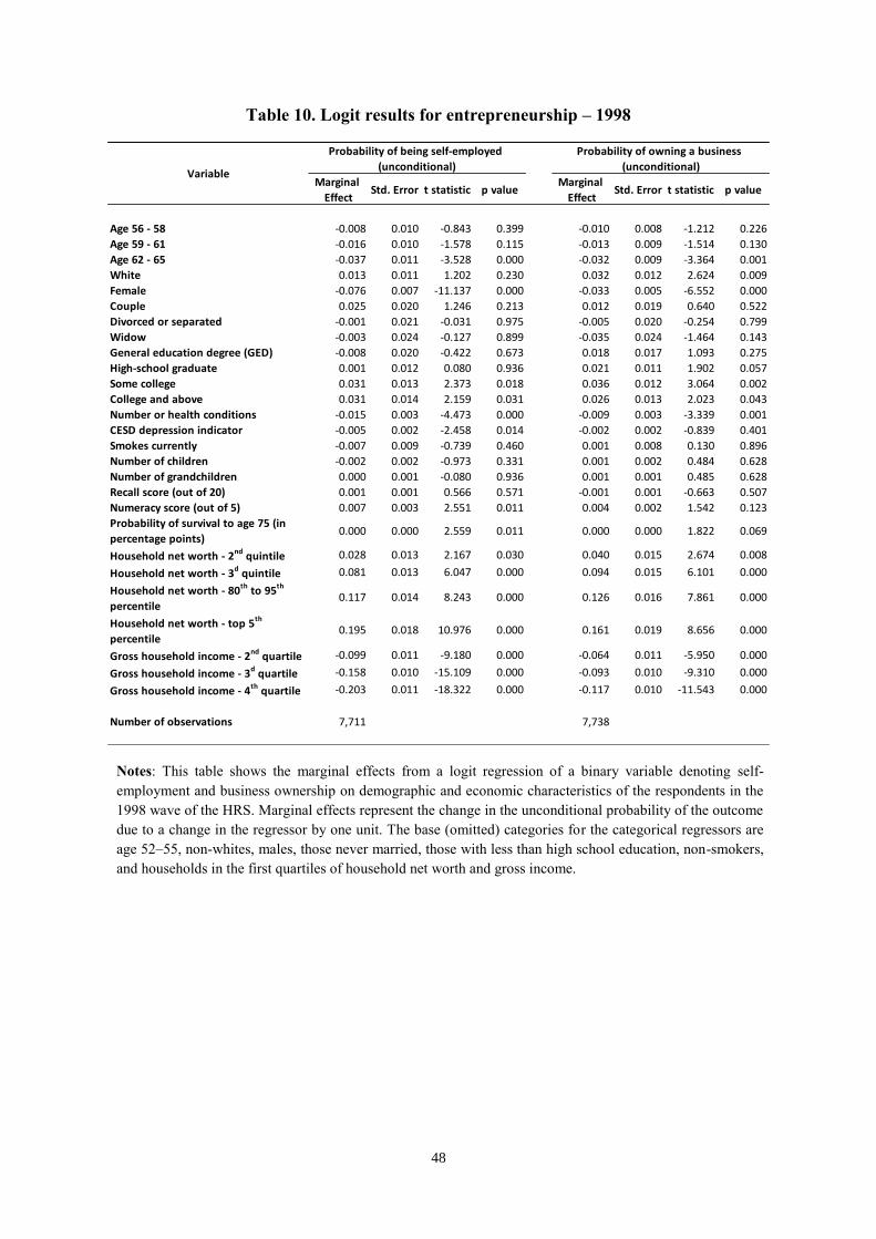
48
Table 10. Logit results for entrepreneurship – 1998
Marginal
EffectStd. Error t statistic p value
Marginal
EffectStd. Error t statistic p value
Age 56 - 58 -0.008 0.010 -0.843 0.399 -0.010 0.008 -1.212 0.226
Age 59 - 61 -0.016 0.010 -1.578 0.115 -0.013 0.009 -1.514 0.130
Age 62 - 65 -0.037 0.011 -3.528 0.000 -0.032 0.009 -3.364 0.001
White 0.013 0.011 1.202 0.230 0.032 0.012 2.624 0.009
Female -0.076 0.007 -11.137 0.000 -0.033 0.005 -6.552 0.000
Couple 0.025 0.020 1.246 0.213 0.012 0.019 0.640 0.522
Divorced or separated -0.001 0.021 -0.031 0.975 -0.005 0.020 -0.254 0.799
Widow -0.003 0.024 -0.127 0.899 -0.035 0.024 -1.464 0.143
General education degree (GED) -0.008 0.020 -0.422 0.673 0.018 0.017 1.093 0.275
High-school graduate 0.001 0.012 0.080 0.936 0.021 0.011 1.902 0.057
Some college 0.031 0.013 2.373 0.018 0.036 0.012 3.064 0.002
College and above 0.031 0.014 2.159 0.031 0.026 0.013 2.023 0.043
Number or health conditions -0.015 0.003 -4.473 0.000 -0.009 0.003 -3.339 0.001
CESD depression indicator -0.005 0.002 -2.458 0.014 -0.002 0.002 -0.839 0.401
Smokes currently -0.007 0.009 -0.739 0.460 0.001 0.008 0.130 0.896
Number of children -0.002 0.002 -0.973 0.331 0.001 0.002 0.484 0.628
Number of grandchildren 0.000 0.001 -0.080 0.936 0.001 0.001 0.485 0.628
Recall score (out of 20) 0.001 0.001 0.566 0.571 -0.001 0.001 -0.663 0.507
Numeracy score (out of 5) 0.007 0.003 2.551 0.011 0.004 0.002 1.542 0.123
Probability of survival to age 75 (in
percentage points)0.000 0.000 2.559 0.011 0.000 0.000 1.822 0.069
Household net worth - 2nd
quintile 0.028 0.013 2.167 0.030 0.040 0.015 2.674 0.008
Household net worth - 3d quintile 0.081 0.013 6.047 0.000 0.094 0.015 6.101 0.000
Household net worth - 80th
to 95th
percentile0.117 0.014 8.243 0.000 0.126 0.016 7.861 0.000
Household net worth - top 5th
percentile0.195 0.018 10.976 0.000 0.161 0.019 8.656 0.000
Gross household income - 2nd
quartile -0.099 0.011 -9.180 0.000 -0.064 0.011 -5.950 0.000
Gross household income - 3d quartile -0.158 0.010 -15.109 0.000 -0.093 0.010 -9.310 0.000
Gross household income - 4th
quartile -0.203 0.011 -18.322 0.000 -0.117 0.010 -11.543 0.000
Number of observations 7,711 7,738
Variable
Probability of being self-employed
(unconditional)
Probability of owning a business
(unconditional)
Notes: This table shows the marginal effects from a logit regression of a binary variable denoting self-
employment and business ownership on demographic and economic characteristics of the respondents in the
1998 wave of the HRS. Marginal effects represent the change in the unconditional probability of the outcome
due to a change in the regressor by one unit. The base (omitted) categories for the categorical regressors are
age 52–55, non-whites, males, those never married, those with less than high school education, non-smokers,
and households in the first quartiles of household net worth and gross income.

49
Table 11. Probit selection model results for entrepreneurship - 2012
Marginal
EffectStd. Error t statistic p value
Marginal
EffectStd. Error t statistic p value
Age 56 - 58 0.030 0.013 2.305 0.021 0.013 0.011 1.265 0.206
Age 59 - 61 0.044 0.014 3.132 0.002 0.005 0.012 0.409 0.682
Age 62 - 65 0.030 0.016 1.881 0.060 0.010 0.013 0.759 0.448
White 0.035 0.012 2.887 0.004 0.055 0.011 5.043 0.000
Female -0.060 0.010 -5.778 0.000 -0.034 0.007 -4.686 0.000
Couple 0.097 0.022 4.311 0.000 0.063 0.019 3.236 0.001
Divorced or separated 0.020 0.023 0.866 0.387 0.019 0.020 0.905 0.365
Widow 0.015 0.033 0.455 0.649 -0.017 0.030 -0.576 0.565
General education degree (GED) 0.045 0.029 1.584 0.113 0.076 0.026 2.907 0.004
High-school graduate 0.035 0.021 1.675 0.094 0.065 0.019 3.354 0.001
Some college 0.068 0.020 3.369 0.001 0.081 0.019 4.173 0.000
College and above 0.075 0.022 3.381 0.001 0.075 0.021 3.618 0.000
Number or health conditions -0.013 0.004 -2.978 0.003 -0.001 0.003 -0.384 0.701
CESD depression indicator -0.003 0.003 -1.041 0.298 -0.003 0.003 -1.085 0.278
Smokes currently -0.008 0.014 -0.584 0.559 -0.004 0.011 -0.345 0.730
Number of children 0.007 0.004 1.788 0.074 0.001 0.003 0.251 0.801
Number of grandchildren -0.001 0.002 -0.682 0.495 0.000 0.001 0.001 0.999
Recall score (out of 20) 0.006 0.002 3.206 0.001 0.002 0.001 1.222 0.222
Numeracy score (out of 5) 0.002 0.004 0.582 0.561 0.002 0.003 0.819 0.413
Probability of survival to age 75 0.000 0.000 1.923 0.055 0.000 0.000 1.523 0.128
Household net worth - 2nd
quintile 0.031 0.015 2.128 0.033 0.043 0.014 3.075 0.002
Household net worth - 3d quintile 0.100 0.016 6.123 0.000 0.096 0.014 6.941 0.000
Household net worth - 80th
to 95th
percentile0.161 0.018 8.843 0.000 0.137 0.015 8.969 0.000
Household net worth - top 5th
percentile0.272 0.030 9.166 0.000 0.180 0.023 7.742 0.000
Gross household income - 2nd
quartile -0.221 0.015 -14.552 0.000 -0.113 0.013 -8.471 0.000
Gross household income - 3d quartile -0.299 0.015 -20.007 0.000 -0.165 0.013 -12.303 0.000
Gross household income - 4th quartile -0.395 0.017 -23.172 0.000 -0.207 0.014 -15.060 0.000
Number of observations 7,918 7,921
Variable
Probability of being self-employed
(conditional on working)
Probability of owning a business
(conditional on working)
Notes: This table shows the marginal effects from a Heckman probit selection model regression of a binary
variable denoting self-employment and business ownership on demographic and economic characteristics of the
respondents in the 2012 wave of the HRS. Marginal effects represent the change in the probability of being self-
employed or an entrepreneur conditional on working in any a capacity due to a change in the regressor by one
unit. The base (omitted) categories for the categorical regressors are age 52–55, non-whites, males, those never
married, those with less than high school education, non-smokers, and households in the first quartiles of
household net worth and gross income.
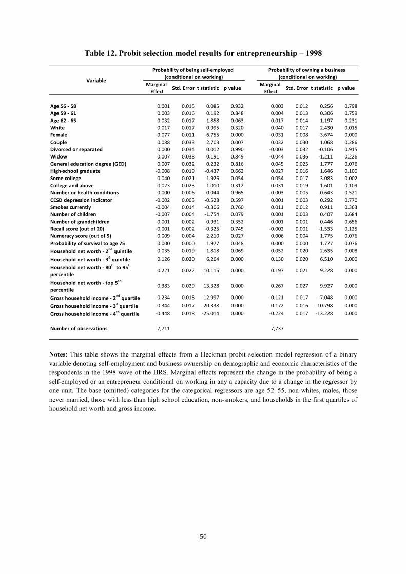
50
Table 12. Probit selection model results for entrepreneurship – 1998
Marginal
EffectStd. Error t statistic p value
Marginal
EffectStd. Error t statistic p value
Age 56 - 58 0.001 0.015 0.085 0.932 0.003 0.012 0.256 0.798
Age 59 - 61 0.003 0.016 0.192 0.848 0.004 0.013 0.306 0.759
Age 62 - 65 0.032 0.017 1.858 0.063 0.017 0.014 1.197 0.231
White 0.017 0.017 0.995 0.320 0.040 0.017 2.430 0.015
Female -0.077 0.011 -6.755 0.000 -0.031 0.008 -3.674 0.000
Couple 0.088 0.033 2.703 0.007 0.032 0.030 1.068 0.286
Divorced or separated 0.000 0.034 0.012 0.990 -0.003 0.032 -0.106 0.915
Widow 0.007 0.038 0.191 0.849 -0.044 0.036 -1.211 0.226
General education degree (GED) 0.007 0.032 0.232 0.816 0.045 0.025 1.777 0.076
High-school graduate -0.008 0.019 -0.437 0.662 0.027 0.016 1.646 0.100
Some college 0.040 0.021 1.926 0.054 0.054 0.017 3.083 0.002
College and above 0.023 0.023 1.010 0.312 0.031 0.019 1.601 0.109
Number or health conditions 0.000 0.006 -0.044 0.965 -0.003 0.005 -0.643 0.521
CESD depression indicator -0.002 0.003 -0.528 0.597 0.001 0.003 0.292 0.770
Smokes currently -0.004 0.014 -0.306 0.760 0.011 0.012 0.911 0.363
Number of children -0.007 0.004 -1.754 0.079 0.001 0.003 0.407 0.684
Number of grandchildren 0.001 0.002 0.931 0.352 0.001 0.001 0.446 0.656
Recall score (out of 20) -0.001 0.002 -0.325 0.745 -0.002 0.001 -1.533 0.125
Numeracy score (out of 5) 0.009 0.004 2.210 0.027 0.006 0.004 1.775 0.076
Probability of survival to age 75 0.000 0.000 1.977 0.048 0.000 0.000 1.777 0.076
Household net worth - 2nd
quintile 0.035 0.019 1.818 0.069 0.052 0.020 2.635 0.008
Household net worth - 3d quintile 0.126 0.020 6.264 0.000 0.130 0.020 6.510 0.000
Household net worth - 80th
to 95th
percentile0.221 0.022 10.115 0.000 0.197 0.021 9.228 0.000
Household net worth - top 5th
percentile0.383 0.029 13.328 0.000 0.267 0.027 9.927 0.000
Gross household income - 2nd
quartile -0.234 0.018 -12.997 0.000 -0.121 0.017 -7.048 0.000
Gross household income - 3d quartile -0.344 0.017 -20.338 0.000 -0.172 0.016 -10.798 0.000
Gross household income - 4th quartile -0.448 0.018 -25.014 0.000 -0.224 0.017 -13.228 0.000
Number of observations 7,711 7,737
Variable
Probability of being self-employed
(conditional on working)
Probability of owning a business
(conditional on working)
Notes: This table shows the marginal effects from a Heckman probit selection model regression of a binary
variable denoting self-employment and business ownership on demographic and economic characteristics of the
respondents in the 1998 wave of the HRS. Marginal effects represent the change in the probability of being a
self-employed or an entrepreneur conditional on working in any a capacity due to a change in the regressor by
one unit. The base (omitted) categories for the categorical regressors are age 52–55, non-whites, males, those
never married, those with less than high school education, non-smokers, and households in the first quartiles of
household net worth and gross income.
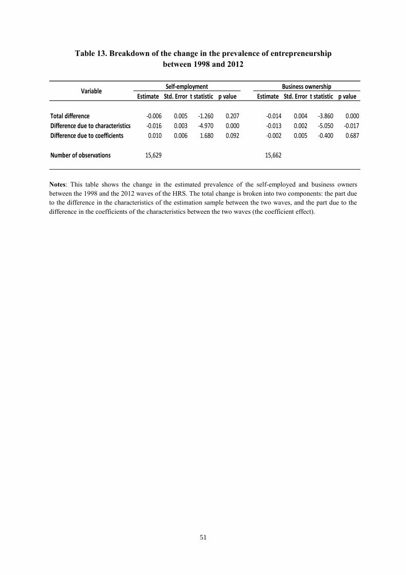
51
Table 13. Breakdown of the change in the prevalence of entrepreneurship
between 1998 and 2012
Estimate Std. Error t statistic p value Estimate Std. Error t statistic p value
Total difference -0.006 0.005 -1.260 0.207 -0.014 0.004 -3.860 0.000
Difference due to characteristics -0.016 0.003 -4.970 0.000 -0.013 0.002 -5.050 -0.017
Difference due to coefficients 0.010 0.006 1.680 0.092 -0.002 0.005 -0.400 0.687
Number of observations 15,629 15,662
VariableSelf-employment Business ownership
Notes: This table shows the change in the estimated prevalence of the self-employed and business owners
between the 1998 and the 2012 waves of the HRS. The total change is broken into two components: the part due
to the difference in the characteristics of the estimation sample between the two waves, and the part due to the
difference in the coefficients of the characteristics between the two waves (the coefficient effect).
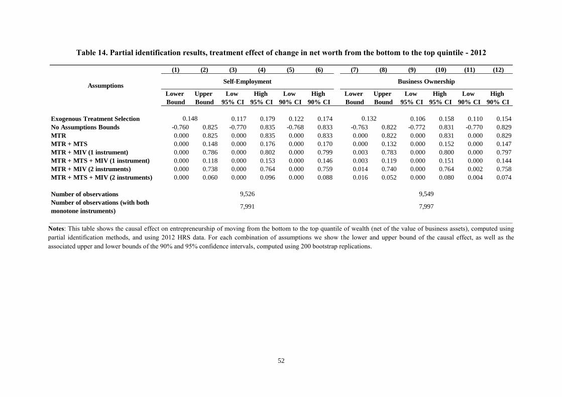
52
Table 14. Partial identification results, treatment effect of change in net worth from the bottom to the top quintile - 2012
(1) (2) (3) (4) (5) (6) (7) (8) (9) (10) (11) (12)
Lower
Bound
Upper
Bound
Low
95% CI
High
95% CI
Low
90% CI
High
90% CI
Lower
Bound
Upper
Bound
Low
95% CI
High
95% CI
Low
90% CI
High
90% CI
Exogenous Treatment Selection 0.117 0.179 0.122 0.174 0.106 0.158 0.110 0.154
No Assumptions Bounds -0.760 0.825 -0.770 0.835 -0.768 0.833 -0.763 0.822 -0.772 0.831 -0.770 0.829
MTR 0.000 0.825 0.000 0.835 0.000 0.833 0.000 0.822 0.000 0.831 0.000 0.829
MTR + MTS 0.000 0.148 0.000 0.176 0.000 0.170 0.000 0.132 0.000 0.152 0.000 0.147
MTR + MIV (1 instrument) 0.000 0.786 0.000 0.802 0.000 0.799 0.003 0.783 0.000 0.800 0.000 0.797
MTR + MTS + MIV (1 instrument) 0.000 0.118 0.000 0.153 0.000 0.146 0.003 0.119 0.000 0.151 0.000 0.144
MTR + MIV (2 instruments) 0.000 0.738 0.000 0.764 0.000 0.759 0.014 0.740 0.000 0.764 0.002 0.758
MTR + MTS + MIV (2 instruments) 0.000 0.060 0.000 0.096 0.000 0.088 0.016 0.052 0.000 0.080 0.004 0.074
Number of observations
Number of observations (with both
monotone instruments)
9,526 9,549
7,991 7,997
AssumptionsSelf-Employment Business Ownership
0.148 0.132
Notes: This table shows the causal effect on entrepreneurship of moving from the bottom to the top quantile of wealth (net of the value of business assets), computed using
partial identification methods, and using 2012 HRS data. For each combination of assumptions we show the lower and upper bound of the causal effect, as well as the
associated upper and lower bounds of the 90% and 95% confidence intervals, computed using 200 bootstrap replications.
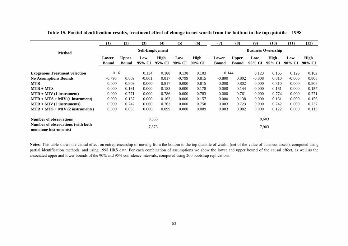
53
Table 15. Partial identification results, treatment effect of change in net worth from the bottom to the top quintile – 1998
(1) (2) (3) (4) (5) (6) (7) (8) (9) (10) (11) (12)
Lower
Bound
Upper
Bound
Low
95% CI
High
95% CI
Low
90% CI
High
90% CI
Lower
Bound
Upper
Bound
Low
95% CI
High
95% CI
Low
90% CI
High
90% CI
Exogenous Treatment Selection 0.134 0.188 0.138 0.183 0.123 0.165 0.126 0.162
No Assumptions Bounds -0.793 0.809 -0.801 0.817 -0.799 0.815 -0.800 0.802 -0.808 0.810 -0.806 0.808
MTR 0.000 0.809 0.000 0.817 0.000 0.815 0.000 0.802 0.000 0.810 0.000 0.808
MTR + MTS 0.000 0.161 0.000 0.183 0.000 0.178 0.000 0.144 0.000 0.161 0.000 0.157
MTR + MIV (1 instrument) 0.000 0.771 0.000 0.786 0.000 0.783 0.000 0.761 0.000 0.774 0.000 0.771
MTR + MTS + MIV (1 instrument) 0.000 0.137 0.000 0.163 0.000 0.157 0.000 0.138 0.000 0.161 0.000 0.156
MTR + MIV (2 instruments) 0.000 0.742 0.000 0.763 0.000 0.758 0.003 0.723 0.000 0.742 0.000 0.737
MTR + MTS + MIV (2 instruments) 0.000 0.055 0.000 0.099 0.000 0.089 0.003 0.082 0.000 0.122 0.000 0.113
Number of observations
Number of observations (with both
monotone instruments)
9,555 9,603
7,873 7,903
MethodSelf-Employment Business Ownership
0.161 0.144
Notes: This table shows the causal effect on entrepreneurship of moving from the bottom to the top quantile of wealth (net of the value of business assets), computed using
partial identification methods, and using 1998 HRS data. For each combination of assumptions we show the lower and upper bound of the causal effect, as well as the
associated upper and lower bounds of the 90% and 95% confidence intervals, computed using 200 bootstrap replications.
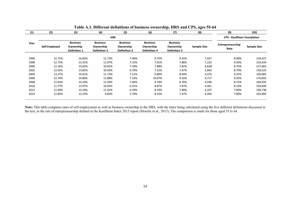
54
Table A.1. Different definitions of business ownership, HRS and CPS, ages 55-64
(1) (2) (3) (4) (5) (6) (7) (8) (9) (10)
Self-Employed
Business
Ownership
Definition 1
Business
Ownership
Definition 2
Business
Ownership
Definition 3
Business
Ownership
Definition 4
Business
Ownership
Definition 5
Sample SizeEntrepreneurship
RateSample Size
1996 12.72% 14.83% 11.72% 7.96% 9.75% 9.35% 7,437 8.98% 118,427
1998 12.75% 13.31% 11.07% 7.15% 7.91% 7.86% 7,222 9.50% 124,634
2000 12.16% 13.65% 10.81% 7.18% 7.88% 7.82% 6,638 8.75% 127,663
2002 12.02% 13.85% 10.43% 6.70% 7.52% 7.47% 5,842 8.79% 158,525
2004 13.27% 14.61% 11.73% 7.21% 9.89% 8.94% 5,476 9.25% 169,085
2006 12.70% 14.80% 11.88% 7.16% 10.07% 9.16% 4,717 9.03% 176,693
2008 12.63% 14.50% 11.50% 7.06% 9.74% 8.76% 4,540 8.72% 184,935
2010 11.77% 13.97% 10.65% 6.41% 8.87% 7.87% 4,461 8.16% 193,849
2012 12.49% 13.59% 11.02% 6.39% 8.74% 7.88% 6,107 7.89% 199,738
2014 11.85% 12.23% 9.82% 5.79% 8.52% 7.47% 6,356 7.80% 203,895
CPS - Kauffman Foundation
Year
HRS
Note: This table compares rates of self-employment as well as business ownership in the HRS, with the latter being calculated using the five different definitions discussed in
the text, to the rate of entrepreneurship defined in the Kauffman Index 2015 report (Morelix et al., 2015). The comparison is made for those aged 55 to 64.
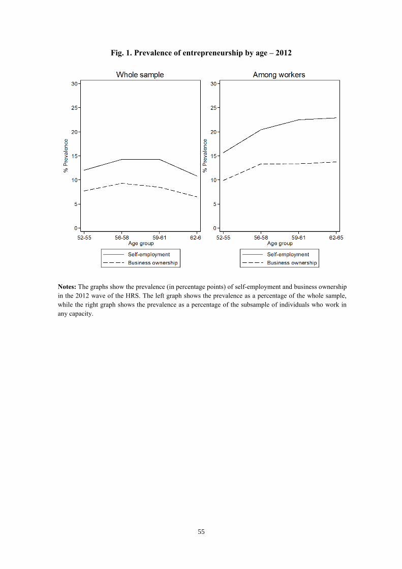
55
Fig. 1. Prevalence of entrepreneurship by age – 2012
Notes: The graphs show the prevalence (in percentage points) of self-employment and business ownership
in the 2012 wave of the HRS. The left graph shows the prevalence as a percentage of the whole sample,
while the right graph shows the prevalence as a percentage of the subsample of individuals who work in
any capacity.
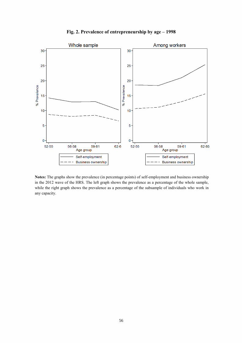
56
Fig. 2. Prevalence of entrepreneurship by age – 1998
Notes: The graphs show the prevalence (in percentage points) of self-employment and business ownership
in the 2012 wave of the HRS. The left graph shows the prevalence as a percentage of the whole sample,
while the right graph shows the prevalence as a percentage of the subsample of individuals who work in
any capacity.

This and other Global Financial Literacy Excellence Center working papers and publications are available online at
www.gflec.org
Global Financial Literacy Excellence Center The George Washington University
School of Business Duquès Hall, Suite 450
2201 G Street NW Washington, DC 20052
P: 202-994-7148 F: 202-994-8289