entitled - utoledo engineeringmjamali/theses/nishatha_thesis.pdfa thesis entitled target tracking...
TRANSCRIPT

A Thesis
entitled
Target Tracking Via Marine Radar
by
Nishatha Nagarajan
Submitted to the Graduate Faculty as partial fulfillment of the requirements for the
Master of Science Degree in Electrical Engineering
_____________________________________
Dr. Mohsin M. Jamali, Committee Chair
_____________________________________
Dr. Peter V. Gorsevski, Committee Member
_____________________________________
Dr. Richard G. Molyet, Committee Member
_____________________________________
Dr. Patricia R. Komuniecki, Dean
College of Graduate Studies
The University of Toledo
December 2012

Copyright 2012, Nishatha Nagarajan
This document is copyrighted material. Under copyright law, no parts of this document
may be reproduced without the expressed permission of the author.

iii
An Abstract of
Target Tracking Via Marine Radar
by
Nishatha Nagarajan
Submitted to the Graduate Faculty as partial fulfillment of the
requirements for the Master of Science in Electrical Engineering
The University of Toledo
December 2012
The growing energy needs have eventually increased the development of wind
turbines. The constructions of wind turbines have several potential impacts of which the
most significant factor is the increasing bird mortality rates due to collision and habitat
loss. Since then, radars have been deployed to study the behavior of birds towards wind
turbines. Radars employ target tracking for identifying the targets (birds) accurately and
efficiently. Several methods of tracking were developed to improve the tracking
efficiency of the radars over the years. Most widely used tracking techniques are Kalman
filter and particle filter. These filters use data with random errors and estimate accurate
values for the current state of the system. Kalman filter is a linear estimator which does
not depend on a set of past observations and hence efficient in real time applications. The
particle filter also known as sequential Monte Carlo method is a nonlinear estimator
which uses a set of particles with various weights for estimation. However, particle filters
have high computation time. Kalman and particle filters were developed over the years
creating various models for various types of systems. A block version of Compressive
Matching Pursuit (CoSaMP) algorithm used in signal reconstruction called BCoSaMP
was employed in tracking. It was seen to give a similar or better performance than

iv
particle filter with less computation time. The BCoSaMP algorithm with Kalman filter
estimation was developed which reduces the mean square error as compared to other
models in certain cases.
This thesis focuses on developing tracker models in radR. Kalman filter tracking
model based on linear data and Gaussian noise that operates over a variety of target
motions and velocities is developed. Particle filter is designed for nonlinear target motion
with non-Gaussian noise. BCoSaMP model that assumes data as sparse is applied for
target tracking and a modified BCoSaMP which replaces least square estimation with
Kalman filter estimation are also implemented. These models were tested with different
data sets and a comparative analysis is performed. The algorithms are tested on simulated
data and marine radar data in radR to compare the effects of the developed tracker
models with the conventional methods in radR. The hybrid algorithm is shown to have
better performance over the other models in the case of simulated track for some targets.
Particle filter has the highest detection rate with marine radar data.

v
Acknowledgements
I am very thankful to the almighty God for everything that I am today
I am most grateful to my advisor Dr. Mohsin Jamali for giving me the opportunity to
work in this project which has been a life cherishing experience. I would like to also
thank Dr. Peter Gorsevski and Dr. Richard Molyet for taking time to serve on my
committee. I am grateful for the continuous support given by Dr. Peter Gorsevski from
Department of Geospatial Sciences at BGSU, Dr. Joseph Frizado from Department of
Geology at BGSU and Dr. Verner Bingman from Department of Psychology at BGSU for
this project which is partially funded by the Department of Energy (Contract #DE-FG36-
06G086096). I would also like to thank all my lab mates especially Todd Schmuland and
Edris Amin for their help and support. I would also like to thank Dr. Jeremy Ross for
contributions to this work.
I am most grateful to know Shavin Thaddeus Shahnawaz and Vivek Sreedhar for all
their guidance and for being there to help me always. I am very lucky to have very
special friends in my life who have always been with me like Praneeth Nelapati, Sakina
Junaghadwala, Sreenadh Reddy, Gubbala Uday Kishore and Midde Vijaya Kumar.
My loving family has been the greatest blessing in my life. I am most thankful to my
loving mother Gajalakshmi and the coolest dad Nagarajan. I am very fortunate to have
the most wonderful sister Yamini Padma and my little brother Akul Akshit.

vi
Table of Contents
Abstract .............................................................................................................................. iii
Acknowledgements………………………………………………………………………..v
Table of Contents ............................................................................................................... vi
List of Tables .....................................................................................................................x
List of Figures ................................................................................................................... xii
1. Introduction……………….. ............................................................................................1
1.1 Methods for Bird Monitoring……………………………………………………...2
1.1.1 Visual Methods………………………………………………………………2
1.1.2 Acoustic Data………………………………………………………………...2
1.1.3 Radio Telemetry……………………………………………………………...3
1.1.4 Cameras………………………………………………………………………3
1.1.5 Radars………………………………………………………………………..4
1.1.5.1 Weather Radars…………………………………………………………5
1.1.5.2 Marine Radars…………………………………………………………6
1.2 Target Tracking……………………………………………………………………6
1.3 Current Research…………………………………………………………………..7
2. Radars in Avian Study………………………………………………………………….8
2.1 Introduction………………………………………………………………………..8
2.2 Marine Radars in Avian Study…………………………………………………….8

vii
2.3 Methods of Reducing Ground Clutter……………………………………………..9
2.4 Analysis of Marine Radar Data………………..……………………….…………9
2.5 Previous Radar Studies……………………………………..…………………...10
2.6 Summary…………..………………………………………………….………….14
3. Marine Radar and Radar Data Processing Software…………………………………..15
3.1 Introduction………………………………………………………………………15
3.2 Marine Radar…………………………………………………………………….16
3.3 Digitizing Card…………………………………………………………………..19
3.4 radR………………………………………………………………………………24
3.4.1 Radar Data Processing…………………………………………………….25
3.4.2 Blip Processing……………………………………………………………..28
3.5 Summary…………………………………………………………………………31
4. Tracker Models in radR……………………………………………………………….32
4.1 Introduction………………………………………………………………………32
4.2 Tracking Techniques…………………………………………………………….33
4.3 Tracker Models in radR………………………………………………………….34
4.4 Tracker Model…………………………………………………………………….35
4.4.1 Nearest Neighbor Model……………………………………………………37
4.4.2 Multi Frame Correspondence Model……………………………………….40
4.5 Summary…………………………………………………………………………46
5. Tracking Algorithms…………………………………………………………………..47
5.1 Introduction……………………………………………………………………....47
5.2 Literature Review of Target Tracking Algorithms………………………………49

viii
5.3 Track Initiation…………………………………………………………………..52
5.4 Data Association…………………………………………………………………53
5.5 Tracking by Data Fusion…………………………………………………………54
5.6 Target Trackers as Estimators……………………………………………………55
5.7 Kalman Filter (KF)………………………………………………………………56
5.7.1 Implementation of Kalman Filter Model in radR…………………………64
5.7.2 Variations of Kalman Filter……………………………………………….70
5.8 Particle Filter…………………………………………………………………….71
5.8.1 Sequential Importance Sampling (SIS)……………………………………72
5.8.2 Implementation of Particle Filter Tracker Model in radR…………………74
5.9 Compressive Sampling…………………………………………………………..80
5.9.1 CoSaMP……………………………………………………………………82
5.10 BCoSaMP………………………………………………………………………83
5.10.1 Algorithm…………………………………………………………………84
5.10.2 Implementation of BCoSaMP Tracker Model in radR…………………..86
5.11 Modified BCoSaMP……………………………………………………………92
5.12 Layout of Tracker Model in radR………………………………………………92
5.12.1 Update Function…………………………………………………………..93
5.13 Development of Tracker Models……………………………………………….94
5.13.1 Kalman Filter Tracker Model…………………………………………….96
5.13.2 Particle Filter Tracker Model……………………………………………..98
5.13.3 BCoSaMP Tracker Model……………………………………………….100
5.13.4 Modified BCoSaMP Tracker Model…………………………………….102

ix
5.14 Summary………………………………………………………………………102
6. Simulations and Results……………………………………………………………...104
6.1 Introduction……………………………………………………………………..104
6.2 Radar Data………………………………………………………………………105
6.3 Simulations of Tracker Models…………………………………………………108
6.4 Simulation of Four Tracker Models with Marine Radar Data………………….128
6.5 Summary………………………………………………………………………..137
7. Conclusion and Future Work………………………………………………………...139
7.1 Conclusion……………………………………………………………………...139
7.2 Future Work…………………………………………………………………….140
References……………………………………………………………………………....141

x
List of Tables
3.1 Models of Furuno Mark 3……………………………………………………………17
3.2 Types of radiator……………………………………………………………………..18
3.3 Specifications of the radar…………………………………………………………...18
3.4 Blip processing parameters…………………………………………………………..28
3.5 Plugins in radR………………………………………………………………………30
4.1 Functions in tracker model in radR………………………………………………….37
4.2 Parameters in the nearesrt neighbor model…………………………………………..40
4.3 Parameters in multi-frame correspondence model…………………………………..44
4.4 Parameters in tracks.csv file…………………………………………………………44
4.5 Sample data in tracks.csv file………………………………………………………..45
5.1 Input and output parameters for Kalman filter………………………………………64
5.2 Input data frame of targets in Kalman filter …..……………………………………..65
5.3 Input and output parameters for particle filter………………………………………75
5.4 Input data frame of targets in particle filter.……….………………………………..75
5.5 Input and output parameters for BCoSaMP…………………………………………87
5.6 Input data frame of targets in BCoSaMP...…………………………………………..87
6.1 Optimized blip processing parameters…………………………………………….129
6.2 Computation time of tracker models……………………………………………….136

xi
List of Figures
1-1 WSR88D data in identification of birds………………………………………………5
1-2 Target detection using marine radar data……………………………………………..6
3-1 Experimental setup…………………………………………………………………..15
3-2 Radar trailer and the slotted array antenna at Bowling Green………………………16
3-3 Parabolic antenna at University of Toledo…………………………………………..17
3-4 Block diagram of XIR3000C………………………………………………………..19
3-5 Heading and bearing signals in radar data…………………………………………..21
3-6 Digitizing card setup…………………………………………………………………21
3-7 Radar data in radar sample application………………………………………………22
3-8 Snapshot of parameters in radar sample application………………………………...23
3-9 Processing of data in radR…………………………………………………………...25
3-10 Blip processing……………………………………………………………………..27
3-11 Sample radar data in radR………………………………………………………….29
3-12 Sample radar data filtered using blip processing in radR………………………….30
3-13 Enabling plugin in radR……………………………………………………………31
4-1 Tracking flight paths of birds using radar…………………………………………...33
4-2 Types of bird tracks………………………………………………………………….33
4-3 Target tracking………………………………………………………………………34
4-4 Tracker models in radR……………………………………………………………..35

xii
4-5 Tracking in radR…………………………………………………………………….36
4-6 Algorithm for tracker model…………………………………………………………37
4-7 Nearest neighbor model with track 1 created using minimum distance ……………38
4-8 Sample data in radR………………………………………………………………….39
4-9 Snapshot of tracks created by nearest neighbor plugin in radR……………………..39
4-10 Digraph with five vertices………………………………………………………….41
4-11 Sample data in radR………………………………………………………………..43
4-12 Snapshot of tracks created by multi-frame correspondence plugin in radR……….43
5-1 Factors influencing tracking………………………………………………………...49
5-2 Track 1 &2 have the same possible target in the next state…………………………53
5-3 Example of target recognition by multiple radars…………………………………...54
5-4 Kalman filter design…………………………………………………………………61
5-5 Flowchart of Kalman filter design…………………………………………………..63
5-6 Input and output parameters for Kalman filter………………………………………64
5-7 Prediction stage in Kalman filter…………………………………………………….65
5-8 Update stage of Kalman filter………………………………………………………..66
5-9 Association of parameters within two stages………………………………………..67
5-10 Implementation of Kalman filter algorithm in radR……………………………….68
5-11 Flowchart of Kalman filter tracker model………………………………………….69
5-12 Kalman filter design in radR……………………………………………………….70
5-13 Sequential importance sampling particle filter……………………………………..74
5-14 Input and output parameters for the particle filter…………………………………74
5-15 Prediction for N particles…………………………………………………………..76

xiii
5-16 Update in particle filter…………………………………………………………….77
5-17 Association of parameters within two stages………………………………………78
5-18 Implementation of particle filter algorithm in radR………………………………..78
5-19 Flowchart of particle filter tracker model…………………………………………..79
5-20 Particle filter design in radR………………………………………………………..80
5-21 Flowchart of BCoSaMP algorithm…………………………………………………86
5-22 Input and output parameters for BCoSaMP………………………………………..87
5-23 Prediction of target position ……………………………………………………….88
5-24 Update in BCoSaMP algorithm……………………………………………………89
5-25 Association of parameters within two stages………………………………………90
5-26 Implementation of BCoSaMP algorithm in radR………………………………….90
5-27 Flowchart of BCoSaMP Model…………………………………………………….91
5-28 Modified BCoSaMP model for tracking…………………………………………...92
5-29 Algorithm of tracker model………………………………………………………..93
5-30 Layout of tracker model in radR……………………………………………………94
5-31 Developed tracker models in radR…………………………………………………95
5-32 Implementation of new algorithm in radR…………………………………………95
5-33 Comparison of current tracker models with Kalman filter…………………………97
5-34 Comparison of current tracker models with particle filter…………………………99
5-35 Comparison of current tracker models with BCoSaMP…………………………..101
5-36 New tracker models in radR………………………………………………………102
6-1 Study area-Ottawa National Wildlife Refugee……………………………………..105
6-2 Single simulated track at constant velocity………………………………………...106

xiv
6-3 Simulated multi-target tracks………………………………………………………106
6-4 Simulated multi-target tracks in radR environment………………………………..107
6-5 Snapshot of marine radar data……………………………………………………...108
6-6 Kalman filter single target tracking………………………………………………...109
6-7 Error rate of Kalman filter………………………………………………………….109
6-8 Multi target tracking using Kalman filter…………………………………………..110
6-9 Error rates for the four tracks………………………………………………………110
6-10 Kalman filter tracker model output in radR……………………………………….111
6-11 Kalman filter tracker model output with noise in radR…………………………..112
6-12 Particle filter single target tracking……………………………………………….113
6-13 Error rate of particle filter…………………………………………………………113
6-14 Multi target tracking using particle filter………………………………………….114
6-15 Error rates for the four tracks……………………………………………………..114
6-16 Particle filter tracker model output in radR……………………………………….115
6-17 Particle filter tracker model output with noise in radR…………………………..116
6-18 BCoSaMP single target tracking…………………………………………………117
6-19 Error rate of BCoSaMP tracking………………………………………………….117
6-20 Multi target tracking using BCoSaMP……………………………………………118
6-21 Error rates for the four tracks……………………………………………………..118
6-22 BCoSaMP tracker model output in radR………………………………………….119
6-23 BCoSaMP tracker model output with noise in radR……………………………...120
6-24 Modified BCoSaMP single target tracking……………………………………….121
6-25 Error rate of modified BCoSaMP tracking……………………………………….121

xv
6-26 Multi target tracking using modified BCoSaMP…………………………………122
6-27 Error rates for the four tracks……………………………………………………..122
6-28 Modified BCoSaMP tracker model output in radR………………………………123
6-29 Modified BCoSaMP tracker model output with noise in radR…………………..124
6-30 Error rates of four tracker models for a single track……………………………...125
6-31 Error rates of track 1 for four tracker models in multi target environment……….126
6-32 Error rates of track 2 for four tracker models in multi target environment……….126
6-33 Error rates of track 3 for four tracker models in multi target environment……….127
6-34 Error rates of track 4 for four tracker models in multi target environment……….127
6-35 Track of the balloon moving away from the radar………………………………..128
6-36 Kalman filter tracking of the balloon……………………………………………..130
6-37 Particle filter tracking of the balloon……………………………………………..130
6-38 BCoSaMP tracking of the balloon……………………………………………......131
6-39 Modified BCoSaMP tracking of the balloon……………………………………...131
6-40 Multi-frame correspondence tracking of the balloon……………………………..132
6-41 Track of the balloon moving towards the radar…………………………………..133
6-42 Kalman filter tracking of the balloon……………………………………………..133
6-43 Particle filter tracking of the balloon……………………………………………...134
6-44 BCoSaMP tracking of the balloon………………………………………………..134
6-45 Modified BCoSaMP tracking of the balloon……………………………………..135
6-46 Multi-frame Correspondence tracking of the balloon…………………………….135
6-47 Number of targets detected……………………………………………………….136

1
Chapter 1
Introduction
One of the major environmental issues of today is the increasing bird mortality rate
due to increase in large scale installation of wind turbines for generation of green energy.
There are 836 bird species in Migratory Bird Treaty Act of which 78 species are
endangered and 14 threatened in U.S. There are also various other reasons for the
increase in bird mortality rate such as cats, tall buildings, power transmission lines and
cell towers. The threat due to wind turbines increases exponentially with the increasing
need for energy [1]. The American Bird Conservancy has reported millions of bird deaths
each year and the deaths due to wind turbines alone contributing to 440,000 per year. The
deaths are caused due to collision or loss of habitat at the constructed site [2]. Due to
these reasons, there have been restrictions to build wind turbines and the necessity to
recognize the low risk sites before construction [3].
The potential wind farm sites generally are avoided if they happen to be stopover
areas used by birds for migration. Appropriate measures are needed to prevent potential
collision with wind turbines before construction. Thus it can be said that the increase in
the need for construction of wind turbines has increased the growth of avian study [1].
Avian study at wind turbines project [4] site help in selecting low risk sites based on:

2
Bird activity.
Migration parameters such as passage rates, altitudes, direction, speed etc.
Type of species and habitat.
1.1 Methods for Bird Monitoring:
Bird monitoring studies may be based on visual methods [5], acoustic signal
recording [6], cameras [7], radio telemetry [8], radars [9] and multiple sensors [10]. An
overview of these methods is provided in the following sections.
1.1.1 Visual Methods:
Direct observation is the oldest methods used for observing bird migrations [11]. A
visual method of monitoring bird densities in an area is called the point count method.
Birds are identified by visual observation or their song. A point count method includes
counting the number of birds in an area of certain radius around the observer. A radius of
20 m is generally used. The point count method helps in differentiating the bird species
and their abundance in an area. The procedure is repeated in the same area for a few days
to improve the accuracy of observations [5]. Bird studies were also conducted by moon
watching. In this method the observations were based on reflections of birds crossing the
disk of the moon [12].
1.1.2 Acoustic Data:
Acoustic data in avian studies were used to identify the species. With the availability
of high end recorders and software for identification, this became a popular method.
There are various software tools available for identifying species based on the spectral
characteristics. The acoustic data helps in providing the number of birds, call patterns and
peak passage rates. A recording system is set up on the wind turbine to collect data. The
3
data consists of bird sounds, turbine noise and other environmental noise. A recognition
system is capable of detecting bird songs and removing all other noise. If a bird is
detected then there is a possibility of occurred collision [6]. Acoustic data is preprocessed
to remove noise and feature extraction techniques are applied for bird detection. Features
may be extracted using Mel-Frequency Cepstral Coefficients (MFCC) [13], wavelet
transforms [14] and other techniques. More recently feature extraction methods such as
Spectrogram-based Image Frequency Statistics (SIFS) and Mixed MFCC and SIFS
(MMS) technique have been used. Extracted features are combined with various
classification methods for identification of birds [15]. A commercially available bat
recognition system such as Sonobat [16] and others [17] can be used for detection of bats.
1.1.3 Radio Telemetry:
Another method of tracking bird flight is by telemetry in which a device is attached to
the bird. In this method a radio transmitter is attached to the bird and the signal is tracked
to study the bird behavior. The radio transmitter consists of a high frequency transmitter,
power supply, antenna and material for mounting. Nowadays Platform Terminal
Transmitters (PTT) and Global Positioning System (GPS) transmitters which use
satellites to relay signals are also used. These transmitters are highly efficient for
monitoring birds. However birds have low survival rate when attached to such devices
[8].
1.1.4 Cameras:
A series of webcams have been used to track birds. The cameras are initially tested to
find limitations with respect to size, velocity and contrast of objects. The data obtained
from the camera is processed with background subtraction, stereo vision and lens

4
distortion techniques for target identification [7]. IR cameras are widely used because the
images are independent of lighting conditions and also provide the temperature
information. In IR cameras, the targets are detected by applying background subtraction
and connectivity of components helps in tracking. The background subtraction techniques
used to detect moving objects are Running Average (RA) [18], Running Gaussian
Average (RGA) [18] and Mixture of Gaussian (MOG) [18]. Thresholding method is
applied to detect birds using an adaptive thresholding of Otsu method called EOtsu which
is an extended version of Otsu method [19]. Then tracking is applied based on the
connectivity of the object. The objects with same area are given same label numbers and
morphology closure operator is used to create a track [20].
1.1.5 Radars:
Discovery of unwanted targets in radar data called as angels led to the evolution of
the study of ornithology [9]. Radars were first used for wind energy related avian study
during mid-1970s. Birds migrate mostly during the night where visual techniques cannot
be applied for detection and hence radars are used. It is also useful when there is less
visibility due to fog or clouds and also for detection over a wider range. Weather and
surveillance radars were used over large areas however high resolution images cannot be
obtained at wind sites and coverage area may not be available near the required wind site.
Marine radars which can provide high resolution image can be very useful. Tracking
radars are also used to track targets by locking the targets position. In the tracking mode,
it gives information on bird flight. In surveillance mode, it uses angle tracking for
multiple targets. Tracking radars are not widely available, expensive and requires
operator training. On the other hand marine radars are commercially available, less

5
expensive and comparatively easy to operate. Therefore marine radars are widely used in
avian study [9].
1.1.5.1 Weather Radars:
The weather radars can also be used to study the bird migration paths. Weather
Surveillance Radars (WSR88D) were established in 1988 for meteorological purposes all
across US. WSR88D is an S band radar and the maximum range coverage is 250 Km
[21]. WSR88D data is widely available and can be exploited to extract biological activity.
The signal processor provides three types of data which is the reflectivity, radial velocity
and spectrum width. The reflectivity and radial velocity data is filtered to detect birds
[22]. Low reflectivity in the image is removed and the radial velocity data is filtered
based on the bird velocity which is greater than insects. The velocity of birds are also
affected by winds that is if the bird is flying along the direction of wind then its velocity
is greater than the speed of tailwind and vice versa. The final targets obtained after
filtering are quantified to study bird densities and flight direction. Figure 1-1 shows the
target identification system used with the weather radar data [23]. However, weather
radars cannot provide a high resolution image at wind energy sites and hence marine
radars were used [9].
Figure 1-1. WSR88D data in identifying birds
WSR88D
Reflectivity
Radial
Velocity
Filtering Target
Identification
6
1.1.5.2 Marine Radars:
Marine radars are widely used in avian study due to their commercial availability,
higher resolution, easy maintenance, dependable, less expensive and provides altitude
information [9] [24].
The target detection in marine radars is difficult due to high amount of clutter and
noise. The ground clutter can be reduced in the marine radar by using protection shield
around the radar beam or by elevating the antenna mount [25]. To study the behavior of
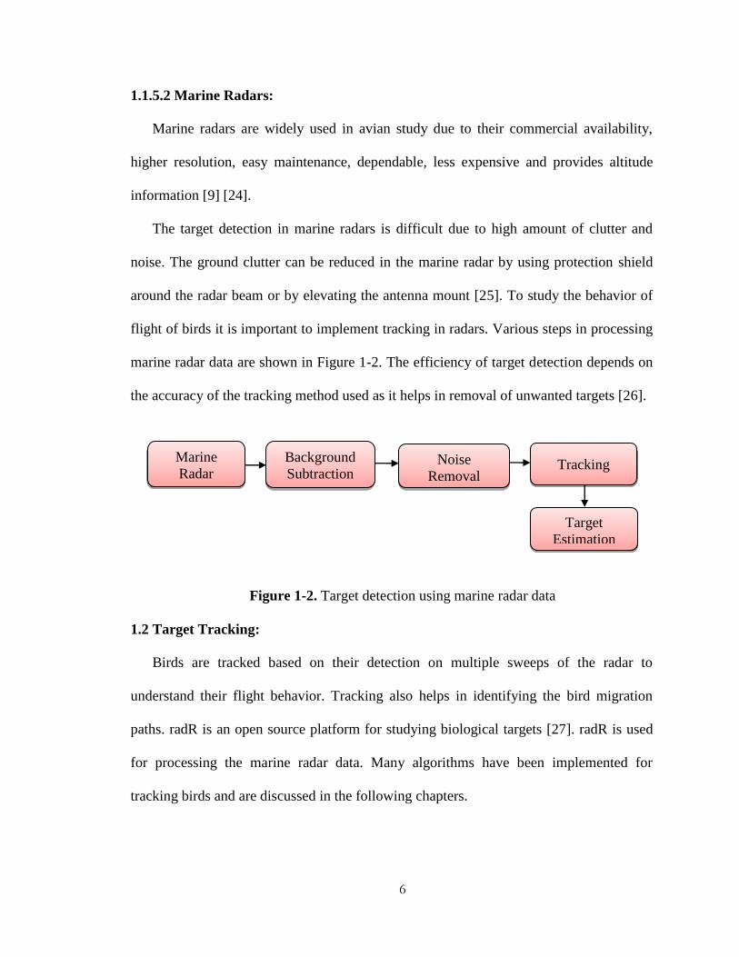
flight of birds it is important to implement tracking in radars. Various steps in processing
marine radar data are shown in Figure 1-2. The efficiency of target detection depends on
the accuracy of the tracking method used as it helps in removal of unwanted targets [26].
Figure 1-2. Target detection using marine radar data
1.2 Target Tracking:
Birds are tracked based on their detection on multiple sweeps of the radar to
understand their flight behavior. Tracking also helps in identifying the bird migration
paths. radR is an open source platform for studying biological targets [27]. radR is used
for processing the marine radar data. Many algorithms have been implemented for
tracking birds and are discussed in the following chapters.
Marine
Radar
Background
Subtraction Noise
Removal Tracking
Target
Estimation

7
1.3 Current Research:
In this research four tracker models have been developed in radR and their
performances with different data sets are compared. Tracker models are Kalman filter,
particle filter, BCoSaMP and modified BCoSaMP. Various chapters in this thesis are
structured as:
Chapter 2: Radars in Avian Study
Chapter 3: Equipment specifications and radR software used for data processing.
Chapter 4: Current tracking models in radR.
Chapter 5: Kalman filters, particle filters and BCoSaMP and modified BCoSaMP are
discussed.
Chapter 6: Simulation of tracker models.
Chapter 7: Conclusions and future work.

8
Chapter 2
Radars in Avian Study
2.1 Introduction
Radars are extensively used in the field of ornithology due to high detection ranges
and ability to detect birds during low visibility conditions. Originally Doppler radars
were used to detect the speed of bird flight. The tracking radars in the non-tracking mode
can help in detecting the density and the altitude of a single target or a flock of birds.
Later studies of tracking birds from reflectivity data were developed. Satellite tracking
radars were also used for wide range target tracking. However, in recent times weather
and marine radars are very popular for the study of bird migration patterns for
quantification of their activity [28].
Radars have the advantage of surveying larger areas beyond the detection capabilities
of visual techniques. They are used for identifying direction and speed of birds. However
a radar cannot recognize bird species or distinguish small birds flying at closer vicinity
from a large bird. Thus radars are used in studies where species identification is not
required [29].
2.2 Marine Radars in Avian Study:
Marine radars are popular in avian study due to their commercial availability, low cost
and higher resolution. Marine radars can be mounted on trailers to study the bird behavior

9
at required locations and clutter reduction screen is placed around the antenna. Shorter
pulse lengths have better target discrimination while long pulse lengths have greater
detection range. Depending on the range the pulse length can be selected. Simultaneous
visual and radar interpretations can be performed for accurate target recognition. Visual
observations are made with the help of binoculars and spotting scope. The target
detection by the radar depends on the settings. The settings of the radar are adjusted
depending on size of target such as large or smaller birds. Based on the sensitivity of the
radar the targets are identified [30]. Initially visual monitoring of the radar data was done
to identify targets and later on image analysis was used to analyze the collected radar
data. The radar data was collected by a personal computer and later image analysis
techniques were applied to analyze and quantify the bird information [29].
Data from the X-band marine radar with T bar antenna in the vertical mode can be
combined with the WSR88D data for the same time period to see any correlation between
two data sets [31]. The T bar antenna can be replaced by a parabolic antenna which can
provide 3D information [32].
2.3 Methods of Reducing Ground Clutter:
Ground clutter in marine radars can be reduced by using a clutter reducing screen
around the antenna. The screen is made of aluminum and is inserted on the lower end of
the antenna at 900 angle. Another method of reducing clutter is by elevating the antenna
by inserting a 50 mm wooden shim which increases the angle of elevation by 100. Twist
the waveguide for further increasing the elevation angle [32].
2.4 Analysis of Marine Radar Data:
Huansheng et al. has used the marine radar for target detection using filtering
10
techniques. The data obtained from the marine radar is the reflectivity information and
bird detection is performed using filtering techniques. Filtering of radar data is
implemented by applying background subtraction, median filtering, segmentation and
morphology [26].
Background subtraction can be applied to remove stationary objects from an image.
There are many background subtraction techniques such as running Gaussian average,
temporal median filter, mixture of Gaussians, Kernel Density Estimation (KDE),
sequential KD approximation, co-occurrence of image variations and Eigen backgrounds
[18]. Principal Component Analysis (PCA) belongs to the Eigen background method and
helps in identifying regular patterns in a data [33]. Random noise can be removed by
applying noise removal techniques such as median filtering, segmentation and image
morphology. Median filtering reduces noise while preserving edges as described by Ziv
Yaniv [34]. Image segmentation and morphology are given by Huang and Wu in [35] and
Wayne, Lin Wei-Cheng and Wu Ja-Ling in [36].
2.5 Previous Radar Studies:
Commercially available Mobile Avian Radar System (MARS) by Geo-Marine uses
X-band marine radar with T-bar antenna operating in vertical and horizontal modes. The
horizontal mode can provide range, direction and speed of the target. Radar in vertical
mode can provide altitude [38].
The types of radars used in the field of ornithology are fan beamed radars and pencil
beamed radars [38]. In 1998 Clemson University Radar Ornithology Laboratory
(CUROL) developed a bird detecting system called BIRDRAD. This consists of
FURUNO 2155BB radar. The T-bar antenna in vertical mode can only provide altitude

11
information of targets within the radar beam. Parabolic antenna was used for three
dimensional tracking of the bird targets [32]. Walls has used two marine radars
simultaneously. He has used X-band in vertical mode and S-band in the horizontal
scanning mode to study bird movements [39]. A custom built converter was used to
digitize the radar pulses and FORTRAN programs were used to obtain pulses that have
recognized targets. The data was stored in an ASCII and processing was done using R
1.9.0 [40].
The radar system was connected to a personal computer and radar data was stored.
Image analysis was then used to remove ground clutter and the birds were categorized
based on the parameters. The clutter can also be removed using the anti-sea clutter which
helps in detecting small targets. In vertical mode when the antenna points to the ground
the energy transmission was disabled using a blind sector [41]. Since slow flying birds
cover the radar viewing range in 30 seconds, therefore the area is scanned by the radar for
every 30 seconds. The birds are classified based on the size using Small-Bird Equivalents
(SBE) and also helps in determining the bird numbers [29]. Radar is calibrated to reduce
sensitivity to remove clutter at closer ranges without affecting the detection of birds [38].
Bertram et al has used FURUNO FR810D (940 MHz, 10 KW, 2 m antenna) marine
radar and has captured radar video using VHS video recorder. Image acquisition system
from the Play Technologies Snappy Video Snapshot has been used. The images were
converted to binary images and a histogram for the image was created. Bird activity was
defined by subtracting the percentage of white pixels from the image when no birds were
present. The bird numbers were estimated based on the area covered by birds by the area
of a known bird [42]. Burger [43] has classified birds into different species based on the

12
speed of flight, path and size. Weber [32] has used track information of targets and has
implemented classification algorithms.
DeTect Inc [44] [45] is developing software to determine wing beat frequency for
identification of bird species. If the bird is tracked by the radar beam then the fluctuations
in the target echo can be used to obtain the wing beat frequency. The wing beat
frequencies help in identifying the species and differentiating birds from bats. Fixed
vertical beam radar with beamwidth large enough to allow large as well as slow moving
birds within the beam for a few seconds is used to measure its wing beat frequency.
Mabee et al. [46] removed insect contamination using air speed. Small targets within
500 m of the radar range and targets with a velocity of <6 m/second has been filtered.
The airspeed is calculated using the formula given in [46]:
√
(2.1)
Where is the airspeed
is the groundspeed
is the wind velocity
is the angle between the target direction and wind vector direction
The target trails is turned on for 30 seconds which is just long enough to find out
direction and speed. Post processing of data is done using SAS V.8 and passage rates are
obtained. The average flight direction is given as [46]:
∑
(2.2)

13
∑
(2.3)
(2.4)
Where is the flight direction at ith
observation
n is the number of observations
Dispersion is calculated as:
Where r =1, when the direction is the same for all observations and r = 0, when there
is uniform distribution [41].
Marine radars have been used for bird detection as well as quantification by
McFarlane et al. [47]. The bird densities are calculated based on the probability of the
target being a bird based on distance between observer and target. Three assumptions
used in this method are certainty of detecting objects at observation point, detecting
objects at initial positions and exact measurements. The densities are quantified as birds
per square kilometer [47]. The wind effects on bird migration are studied as it has greater
influence on bird flights compared to other variables. The winds increase the ground
speed of birds and also causes drift in the migration path as reported by Kerlinger et. al.
[48].
Gauthreaux et al. [28] has equipped radar with a Geographical Positioning System
(GPS) to locate the latitude and longitude of the target. The marine radar results are
correlated with the WSR 88D data [28]. Gauthreaux et al. [49] have developed another
method of validation by comparing vertically pointing fixed beam radar with the thermal
camera data.

14
2.6 Summary:
Radars used in avian study and the extensive usage of marine radars in the field of
ornithology were discussed. Various techniques implemented to reduce clutter and the
data processing methods for bird identification in the marine radar data is also discussed.
The 3-D information of targets is obtained using a parabolic antenna and the t-bar
antenna can be used in the vertical mode to extract the altitude information of birds. In
the following chapter the experimental setup to collect data using marine radar and the
data processing software radR is discussed in detail. The processing of data in radR to
extract bird targets relies on various filtering parameters.

15
Chapter 3
Marine Radar and Radar Data Processing Software
3.1 Introduction
Marine radar is used for bird observation and quantification of their activity. The
radar data is collected using a digitizing card XIR3000B from Russell Technologies as
the slave display. The data collected is processed using open source radR software for
target detection and tracking. The experimental setup of the entire system is shown in
Figure 3-1. The marine radar is run all through the night from evening civil twilight to
morning civil twilight.
Figure 3-1. Experimental setup
The marine radar is connected to the digitizing card and as the antenna rotates the
signal is transmitted to the digitizer. The received signal is digitized and transmitted to a
16
laptop/PC through the USB and data is collected using radar sample application provided
by SDK of the XIR3000 card. radR is used for real time processing or post processing of
the saved files.
3.2 Marine Radar:
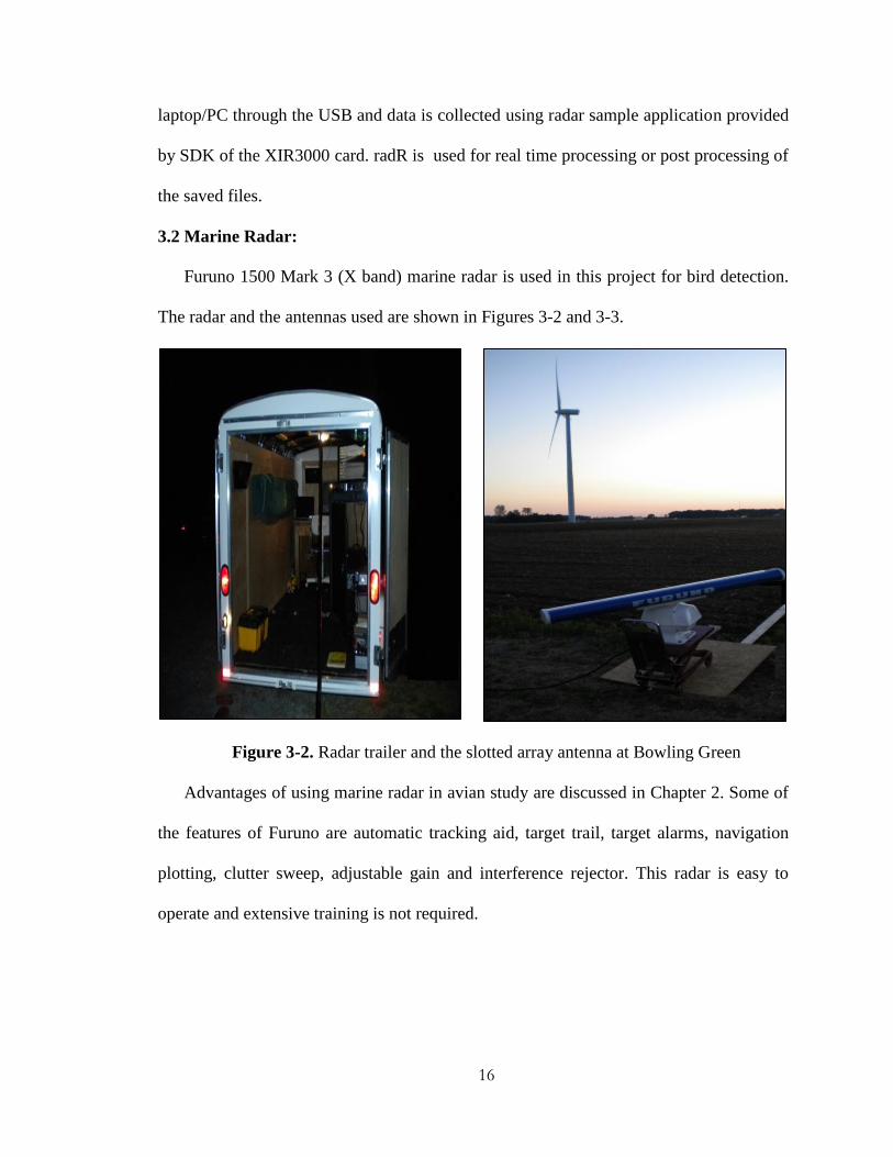
Furuno 1500 Mark 3 (X band) marine radar is used in this project for bird detection.
The radar and the antennas used are shown in Figures 3-2 and 3-3.
Figure 3-2. Radar trailer and the slotted array antenna at Bowling Green
Advantages of using marine radar in avian study are discussed in Chapter 2. Some of
the features of Furuno are automatic tracking aid, target trail, target alarms, navigation
plotting, clutter sweep, adjustable gain and interference rejector. This radar is easy to
operate and extensive training is not required.

17
Figure 3-3. Parabolic antenna at University of Toledo
There are different models of Furuno marine radars available which are given in
Table 3.1. These models are classified based on the input power and the radiator model.
Table 3.1: Models of Furuno Mark 3
Radar Model Power (KW) Radiator Type
FR- 1505 Mark 3 6 XN12AF,XN20AF
FR- 1510 Mark 3 12 XN12AF,XN20AF
FR- 1525 Mark 3 25 XN20AF
Radiators are available in various lengths and appropriate length should be selected
based on application. Specifications for different types of slotted waveguide are given in
Table 3.2.

18
Table 3.2: Types of radiator
Radiator Type XN12AF XN20AF XN24AF
Length (Ft.) 4 6.5 8
Beamwidth (H) 1.80
1.230
0.950
Beamwidth (V) 200
Sidelobe 100 -28 dB
Polarization Horizontal
Specifications of Furuno Mark 3 radar are given Table 3.3. It has an Automatic
Tracking Aid (ATA) which can plot up to 20 targets and the Electronic Plotting Aid
(EPA) allows plotting tracks for 10 targets. The radar map provides the geographical
information of the area.
The antennas used were slotted array and the parabolic antenna. The slotted array
antennas are widely used in navigation system due to emission of linear polarized waves
and greater efficiency.
Table 3.3: Specifications of the radar
Specifications of Marine Radar
Frequency 9410 MHz ± 30 MHz (X-band)
IF 60 MHz
Noise Figure 6 dB
Range Accuracy 1% Maximum Range
Bearing Accuracy ± 10
EPA 10 targets
ATA 20 targets
During the migratory seasons the data is collected using the acquired marine radar.
The data collection is divided into three time slots which are evening civil twilight,
morning civil twilight and night time observations. The slotted array antenna is used
during the morning and evening civil twilights with the antenna rotation around the
horizontal axis, it is the time when the birds ascend and descend. The horizontal beam
19
width is 1.230 and provides greater target discrimination, detectability and higher
resolution. This mode helps in detecting the height of targets and hence the ascend and
descend of targets can be detected accurately. The night time observations are performed
using the parabolic antenna which covers wider area and target are detected along with
heights and angle of arrival [50] [51].
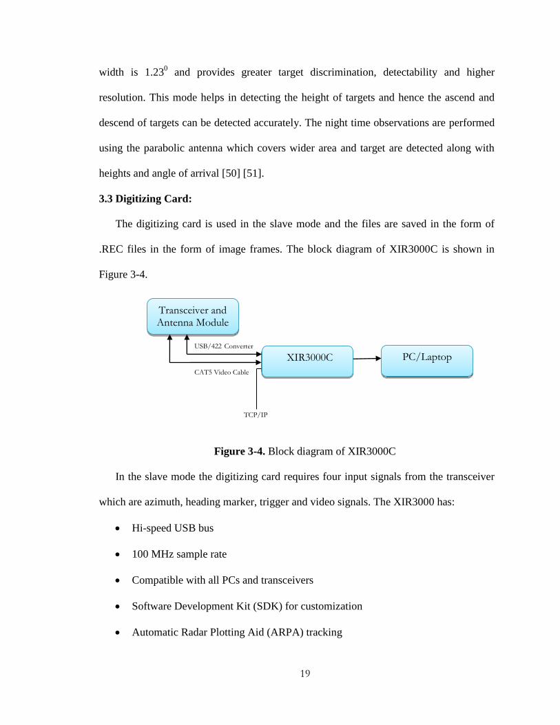
3.3 Digitizing Card:
The digitizing card is used in the slave mode and the files are saved in the form of
.REC files in the form of image frames. The block diagram of XIR3000C is shown in
Figure 3-4.
Figure 3-4. Block diagram of XIR3000C
In the slave mode the digitizing card requires four input signals from the transceiver
which are azimuth, heading marker, trigger and video signals. The XIR3000 has:
Hi-speed USB bus
100 MHz sample rate
Compatible with all PCs and transceivers
Software Development Kit (SDK) for customization
Automatic Radar Plotting Aid (ARPA) tracking
TCP/IP
USB/422 Converter
CAT5 Video Cable
Transceiver and Antenna Module
XIR3000C PC/Laptop

20
Ethernet with TCP/IP
The Russell Technologies Inc. Software Development Kit (RTI SDK) allows
flexibility in scale, image and display options. The SDK has following features:
Header, RTI DLL and library files
Radar sample application which allows viewing and saving of radar images
MS VC++ sample files
Clutter and interference suppression
Antenna Control Module (ACM)
The radar sample helps in displaying, saving and playback of files in the form of .REC
files. The .REC files can be processed using radR software developed for detecting
biological targets [52]. In this project XIR3000B digitizing card is used in slave mode
and has an input power of 12V. It is connected to the power supply at the transceiver and
the four input signals are initialized. The four input signals from the transceiver to the
digitizing card are:
Heading Marker: This signal appears once every sweep of the antenna and shows
the correct alignment of the antenna.
Trigger: This signal gives the time for the transceiver to transmit which helps the
XIR3000 card to start digitization process of the received signal.
Bearing: This gives the direction of the target.
Video: This is the data received by the digitizing card. Figure 3-5 shows the
heading marker and the bearing in radar data.

21
Figure 3-5. Heading and bearing signals in radar data
If these signals are not received correctly then ‘missing’ appears next to the signal in the
radar sample software [53].
The connections of the digitizing card in the slave mode are shown in Figure 3-6. The
input of the digitizing card is connected to the transceiver and the output is an USB
connection to the laptop or PC with radar sample application.
Figure 3-6. Digitizing card setup
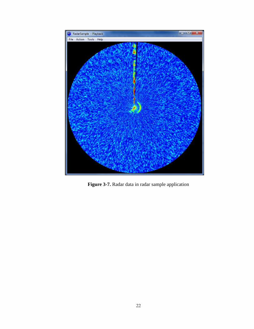
The snapshot of radar sample application is given in Figure 3-7 and the parameters
are shown in Figure 3-8 [52].
Target 1
Transceiver XIR3000B (Slave Mode)
PC/Laptop
4 input signals
12V DC USB
22
Figure 3-7. Radar data in radar sample application

23
Figure 3-8. Snapshot of parameters in radar sample application

24
3.4 radR:
radR is an open source software used for studying biological targets. The software
was developed by Taylor et al. It is easily down loadable and John Brzustowski of radR
development team happily provides answers to questions. radR is used for real time target
recognition and tracking developed using R language works with both Windows and
Linux operating systems [27]. This was especially designed for radar data processing. R
language is an extension of S language developed by Bell Laboratories [27]. The
programs are written in R and C language and interface is coded using tcl/tk by which
each scan of the radar data is processed and possible targets (blips) are obtained by noise
removal. radR has many plugins of which the ones used in the project are plugin for
reading the .REC files, antenna orientation, noise removal, blip processing, saving blips
and target tracking.
radR is not only used for post processing and saving files but also for real time
tracking. The radar data is processed in radR by setting the antenna parameters and
selecting the XIR3000 plugin for reading the data from the digitizing card. The data can
be saved by radR as a blip movie which contains only blips information. The XIR3000
plugin was developed for the XIR3000 digitizing card by Russell Technologies SDK and
similar plugins for acquiring data using other digitizing cards can also be developed [27].
radR is very useful for saving data in blip movie format which contains only the
required target information and the unwanted noise is removed thus saving memory in
the case of large data files. The steps for processing data in radR are shown in Figure 3-9
which shows the key steps involved in processing files that is parameter initialization,
plugin selections and saving output files.

25
Figure 3-9. Processing of data in radR
3.4.1 Radar Data Processing:
Initial steps involve running the batch file, antenna selection and XIR3000 reader
plugin. The data is read by the .REC file reader plugin called XIR3000. Initially the radR
application is launched and then the XIR3000 plugin is enabled which helps in batch
processing of the files. The antenna is selected based on the type of antenna, the beam
widths, angle above the ground and axis of rotation. Select the blip processing window
and set parameters for noise removal such as selecting the number of learning scans,
noise threshold, hot score and cold score, cell size and filtering based on a logical
expressing, minimum blip area, maximum blip area, minimum number of samples and
maximum number of samples, this process is called blip extraction. Adjacent hot cells are
called patches and those that satisfy the criteria of blips are saved as blips.
Step 1
• Run radR batch file
• Set antenna parameters
Step 2 • Load plugins required for processing
• Set parameters for blip processing
Step 3
• Run the data
• Save the processed data

26
Learning scans are the number of scan used in background subtraction technique. Hot
score and cold score are thresholds which differentiate bird targets from the background
noise. The blip area such as minimum and maximum area in meters square is defined.
Old stats weighing is a parameter that defines weights between past and present frame’s
background mean and mean deviances. Samples are the echo strength digitized sequence.
It is given in terms of d bits per sample giving a sample range from 0 to . Samples
per cell are the number of rows in one stats cell and pulses per cell are the number of
columns of one stats cell. The angular span is the number of columns along the angular
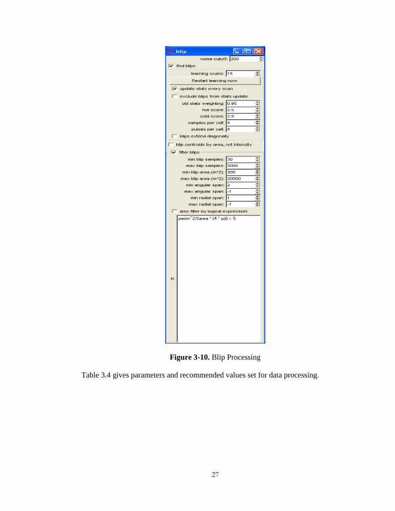
area and radial span is the number of rows along the range. Blips maximum and
minimum area in terms of square meters can be defined to remove large targets. Further
filtering of blips can be specified by a filtering criteria based on formulas defining the
targets. Cells that satisfy all the filtering criteria specified forms a blip. Figure 3-10 shows
blip processing given by radR.
27
Figure 3-10. Blip Processing
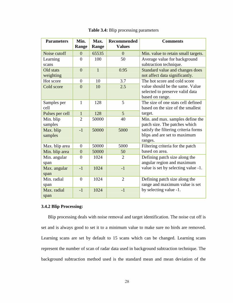
Table 3.4 gives parameters and recommended values set for data processing.
28
Table 3.4: Blip processing parameters
Parameters Min.
Range
Max.
Range
Recommended
Values
Comments
Noise cutoff 0 65535 0 Min. value to retain small targets.
Learning
scans
0 100 50 Average value for background
subtraction technique.
Old stats
weighting
0 1 0.95 Standard value and changes does
not affect data significantly.
Hot score 0 10 3.7 The hot score and cold score
value should be the same. Value
selected to preserve valid data
based on range.
Cold score 0 10 2.5
Samples per
cell
1 128 5 The size of one stats cell defined
based on the size of the smallest
target. Pulses per cell 1 128 5
Min. blip
samples
2 50000 40 Min. and max. samples define the
patch size. The patches which
satisfy the filtering criteria forms
blips and are set to maximum
ranges.
Max. blip
samples
-1 50000 5000
Max. blip area 0 50000 5000 Filtering criteria for the patch
based on area. Min. blip area 0 50000 50
Min. angular
span
0 1024 2 Defining patch size along the
angular region and maximum
value is set by selecting value -1. Max. angular
span
-1 1024 -1
Min. radial
span
0 1024 2 Defining patch size along the
range and maximum value is set
by selecting value -1. Max. radial
span
-1 1024 -1
3.4.2 Blip Processing:
Blip processing deals with noise removal and target identification. The noise cut off is
set and is always good to set it to a minimum value to make sure no birds are removed.
Learning scans are set by default to 15 scans which can be changed. Learning scans
represent the number of scan of radar data used in background subtraction technique. The
background subtraction method used is the standard mean and mean deviation of the
29
learning scans. Further filtering can be performed by selecting appropriate values for hot
score, cold score, area of the target and also with logical expressions.
Blips exceeding the user defined z-score value (threshold) are marked as hot.
Adjacent hot cells are combined and those that meet the filtering criteria are called blips.
Display options can be set to create blip trails of targets and colors for the display.
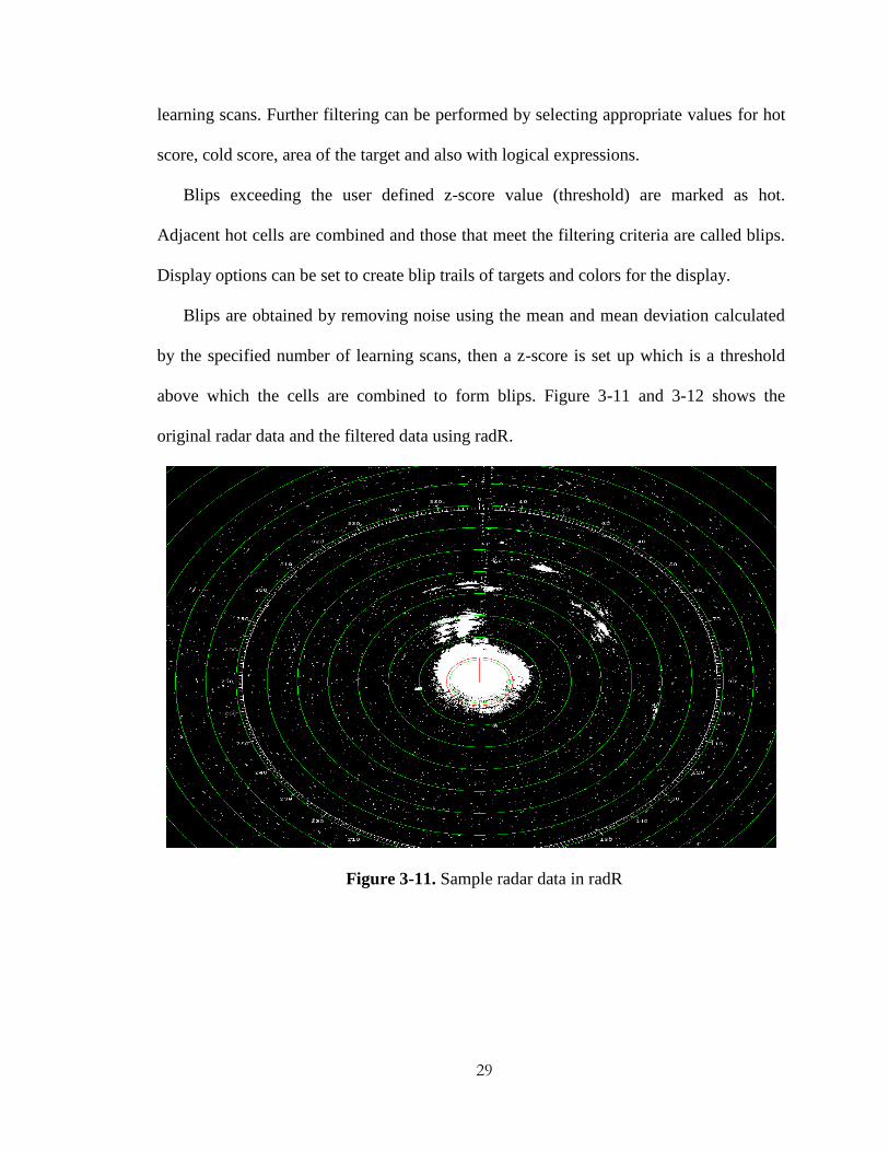
Blips are obtained by removing noise using the mean and mean deviation calculated
by the specified number of learning scans, then a z-score is set up which is a threshold
above which the cells are combined to form blips. Figure 3-11 and 3-12 shows the
original radar data and the filtered data using radR.
Figure 3-11. Sample radar data in radR

30
Figure 3-12. Sample radar data filtered using blip processing in radR
A console window is present in radR which helps in running commands while radR is
running or to run scripts on radR. The processed data can be saved in a movie format or
in a CSV file using save blips plugin. In Table 3.5, a list of radR plugins and their
applications are described [54].
Table 3.5: Plugins in radR
Plugins Applications
antenna Antenna selection
seascan Obtain data from Rutter Inc. Sigma S6 digitizing card
seascanarch Reads data saved by Rutter seascan software
xir3000 Obtain data from Russell Technologies Inc. XIR3000 USB video
processor
xir3000arch Reads data saved by RTI software
video Reads video data
declutter Noise removal
tracker Creating tracks of targets
zone Excludes data within the defined region
genblips Generation of artificial blips
saveblips Save blip information in .blips file
blipmovie Save data in blip movie format

31
Figure 3-13 shows a snapshot of enabling a plugin in radR.
Figure 3-13. Enabling plugin in radR
3.5 Summary:
The marine radar and the digitizing card XIR3000B used in the project are discussed.
The radar data is processed using radR software. Various plugins in radR and the
importance of blip processing parameters for accurate target identification is given in
detail. The following chapter discusses tracking and the current tracker models in radR.

32
Chapter 4
Tracker Models in radR
4.1 Introduction
Tracking provides the current and estimated flight path of any target of interest.
Tracking targets using radars may be very challenging due to the randomness of the data
and presence of large amount of noise commonly known as clutter. Tracking can also be
considered as filtering operation for removal of unwanted targets. Due to the randomness
in the radar data, tracking algorithms play a vital role in target detection and clutter
removal. This work focusses on analysis of the behavior of birds toward man-made
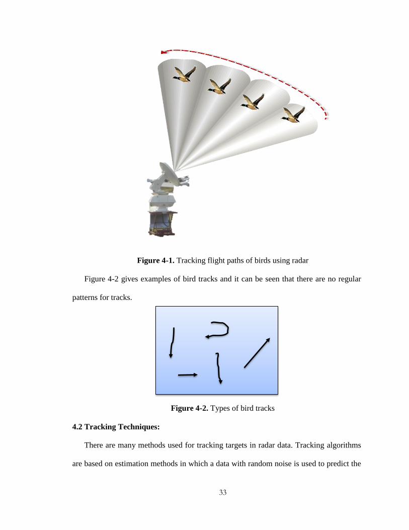
structures. Tracking will be used to determine bird migration patterns. Figure 4-1 shows
tracking of birds using radar.
33
Figure 4-1. Tracking flight paths of birds using radar
Figure 4-2 gives examples of bird tracks and it can be seen that there are no regular
patterns for tracks.
Figure 4-2. Types of bird tracks
4.2 Tracking Techniques:
There are many methods used for tracking targets in radar data. Tracking algorithms
are based on estimation methods in which a data with random noise is used to predict the

34
position of the target in the next time interval. Tracking methods use initial position,
velocity and acceleration and predict future position of the target. The efficiency of the
tracking method depends on the accuracy of initial conditions and the assumptions made
during their design. There are many methods that have been developed for different
systems, sources and target conditions. Some of the tracking techniques are maximum
likelihood, Bayes estimators, maximum a posteriori, minimum variance unbiased
estimator, Kalman filter, particle filter and Weiner filter [55].
4.3 Tracker Models in radR:
Tracking radars operate on the principle of locking the target's position and moving
along with it. It uses track while scan approach by which multiple targets are tracked by
search and scan technique [56]. Marine radars operate in surveillance mode and requires
target tracking algorithm for generation of target tracks. Figure 4-3 shows steps involved
in target tracking.
Figure 4-3. Target Tracking
Input target parameters
Track Initiation
Tracking Algorithm
Data Association
𝜃
Track 1
Track 2 Track 3
Track 1
Track 2
Track 3
Track 1
Track 2
Track 3

35
radR is used for processing radar data which is an open source software available for
recording and processing radar data. It has algorithms for recording, detecting, tracking
and saving target information. The tracker plugins currently in radR are the nearest
neighbor model and the multi-frame model. The nearest neighbor tracking is based on
minimum distance and multi-frame tracking is based on maximum gain. Figure 4-4
shows the two current tracker models in radR [54].
Figure 4-4. Tracker models in radR
Radar data processing via radR utilizes number of plugins. First of all the tracker
plugin is enabled and the appropriate tracker model is selected. The velocity of targets to
be tracked and the number of blips required to form a track can be selected in order to
remove unwanted targets. Run the data using the player and tracks are created as the files
are processed. The data is saved in the tracks.csv files with all the blip information such
as time stamp, track number, scan number, blip number, x-coordinates, y-coordinates, z-
coordinates, intensity, area, perimeter, radial span, angular span and number samples of
each blip.
4.4 Tracker Model:
The tracker model reads the previous frames as old data points. Current frame data is
stored as blips. The tracker model then uses current blips and performs matching with
previously stored blips. Tracks with matched blips are stored in the gain function. Blips
Tracker Models
Nearest Neighbor Model
Multi frame Model

36
without any match start their own track. The gain function is read by the tracker plugin
and tracks are plotted on the radR plot window. Figure 4-5 shows steps involved in radR.
Figure 4-5. Tracking in radR
The tracker model consists of various functions as shown in Table 4.1. Each function
performs a unique task. The update function updates each track by adding blips to the
existing track or starting a new track. The tracker algorithm is implemented in the update
function where matched blips are selected and are given in the form of gain function
which stores the column index of the matched blips. Get menu function obtains the user
input for controlling the tracking procedure based on the minimum number of blips
required to form a track and maximum speed. Set blip fresh time selects the expiry time
of the track and if the controls are changed while running the data then the tracks are
refreshed. Other functions are used to define the maximum speed of the track, select,
deselect, load and unload a plugin. Figure 4-6 shows the layout of the tracker model file
in radR.
Old point
(Previous frame)
Blips
(Current frame)
Tracker model
Track matches
(Gain function)
Tracker plugin

37
Table 4.1: Functions in tracker model in radR
Functions Comments
Update Tracking algorithm identifies best matched blip for each track.
Get menu It is used to control parameters to create track dynamically.
Select Select function defines the onset of a track.
Deselect Deselect function defines the expiry time for a track.
Load Load is used to enable the tracker model.
Unload Unload is used to disable a tracker model.
Set blip fresh time Defines the time for which a blip is retained in the frames.
Set track stale time Defines the time for which a track is active.
Figure 4-6. Algorithm for tracker model
4.4.1 Nearest Neighbor Model:
The nearest neighbor plugin creates tracks based on the minimum distance between
blips of the current frame to the ones on the previous frame [57]. Filtering is performed
based on velocity, turning angle and the blip size. Distance is calculated between blips in
the current and previous frames. All possible combination of distances is stored in a
Get menu function
Select function
Deselect function
Load function
Unload function
Set blip fresh time function
Set track stale time function
Update function Adds blips to tracks
Assign parameters
for track
Track onset
Track expiry
Load a plugin
Unload a plugin
Active blip time
Active track time
38
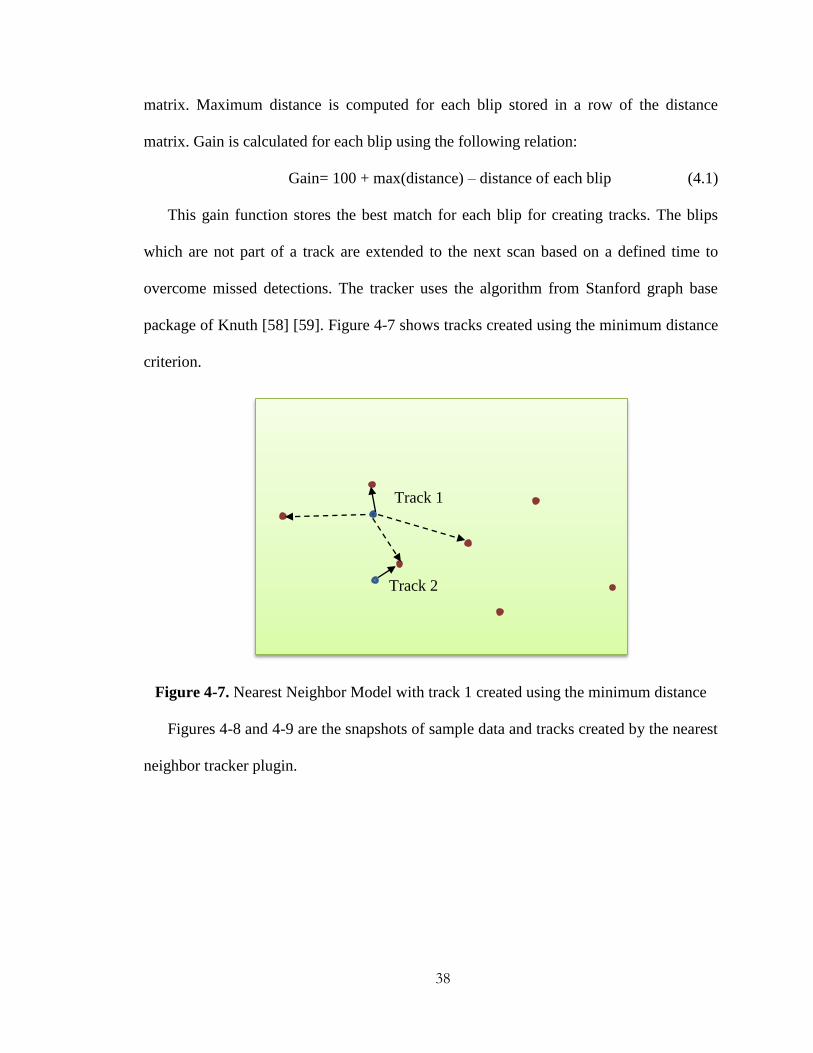
matrix. Maximum distance is computed for each blip stored in a row of the distance
matrix. Gain is calculated for each blip using the following relation:
Gain= 100 + max(distance) – distance of each blip (4.1)
This gain function stores the best match for each blip for creating tracks. The blips
which are not part of a track are extended to the next scan based on a defined time to
overcome missed detections. The tracker uses the algorithm from Stanford graph base
package of Knuth [58] [59]. Figure 4-7 shows tracks created using the minimum distance
criterion.
Figure 4-7. Nearest Neighbor Model with track 1 created using the minimum distance
Figures 4-8 and 4-9 are the snapshots of sample data and tracks created by the nearest
neighbor tracker plugin.
Track 1
Track 2

39
Figure 4-8. Sample data in radR
Figure 4-9. Snapshot of tracks created by Nearest Neighbor Plugin in radR
User selectable parameters in the nearest neighbor model in radR are given in Table
4.2.

40
Table 4.2: Parameters in the nearest neighbor model
Parameter Min.
Range
Max.
Range
Recommended
Values
Comments
How long a blip is
retained as a
possible track
starter
1 3600 4 Time for retaining blips
to find matches in
seconds.
How long track
stays active after
last blip
1 3600 10 Time to preserve a
track in seconds.
Maximum turning
rate (degrees per
second)
0 180 20 Turning rate is set to
remove fast
maneuvering targets.
Maximum rate of
change of blip area
(percent/s)
0 300 150 Rate of change of blip
area that are added to
tracks.
Maximum rate of
change of blip
intensity (percent/s)
0 300 150 Rate of change of blip
intensity that are added
to tracks
4.4.2 Multi Frame Correspondence Model:
This is a non-iterative greedy algorithm which matches targets based on a gain
function. The blips with maximum gain are added to the tracks [60]. Assume that the
length of the track to be T for m-points. In each track the first point has no backward
correspondence and the last point has no forward correspondence. Set of tracks for m-
points are given as:
A = (4.2)
Where A is a set of tracks for m-points in the frame F
is the track for each point
If , then it is said
is a response of a sensor or if then
is
due to sensor noise. D = (V, E) represents edge weighted graph where V is the vertices
and E is the edge of digraph D. In this graph, a directed path P is the number of
connected vertices of length k. Vertex disjoint path is denoted by c and is a path of

41
digraph D such that any path of c contains all the vertices of D and c does not have a
common vertex for any two paths. W(c) represents weights of all edges in c. The path
with the maximum weight is selected as a match or gain function. Figure 4-10 shows an
example of digraph. In this example there are five vertices V= a, b, c, d, e and assume
each edge with weight 1. A path for the graph from vertex a to c is given as P= a, b, c.
Consider the vertex c and the different paths to c from four vertices are Pa= a, b, c, Pb=
b, c, Pd= d, e, a, b, c or d, e, b, c and Pe= e, b, c. For each path cover, weights
are calculated and the path with maximum weight is selected.
Figure 4-10. Digraph with five vertices
Matching is performed corresponding to the maximum weight. Gain contains weights
of the digraph. Greedy algorithm is used to find the maximum weight path assuming
points in frame F are available up to time and gets updated as more frames are
available. Thus for every additional frame, tracks are extended to the new frame.
Algorithmic steps for multi-frame correspondence method are:
Step 1: Assume two frames, let r = 2
For each additional frame
Step 2: Create extension digraph D for the frames.
Step 3: Compute weights of edges using gain function
Step 4: For graph D calculate the maximum path.
Step 5: Replace false hypotheses
a
b c
d e

42
Step 6: backtracking is performed
Step 7: Increment r
End for loop
False hypothesis can be replaced using two methods namely false hypothesis
replacement and non-recursive false hypothesis replacement. False hypotheses
replacement deletes the false hypothesis from graph and the graph is checked again for
matches between all frames. The non-recursive false hypothesis replacement deletes the
false hypothesis and two-frame correspondence is solved. False hypothesis is replaced if
the gain is above the threshold value and its value is set to one otherwise it set to zero.
Gain function is given by the distance between actual positions to the predicted
position. It helps in obtaining matches close to the predicted value which is similar to the
nearest neighbor however the direction of motion is not considered which gives rise to
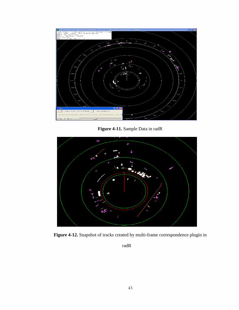
irregular paths [60]. The sample data and snapshot of multi-frame correspondence
tracking in radR are shown in Figures 4-11 and 4-12. User selectable parameters in the
multi-frame correspondence model in radR are given in Table 4.3.
43
Figure 4-11. Sample Data in radR
Figure 4-12. Snapshot of tracks created by multi-frame correspondence plugin in
radR

44
Table 4.3: Parameters in multi-frame correspondence model
Parameter Min.
Range
Max.
Range
Recommended
Values
Comments
Number of scans
to backtrack
2 100 2 For each additional scan the
tracks can be corrected by
backtracking.
Weight of
directional
coherence Vs.
proximity to
prediction
0 1 0.5 Parameters is set to 0.5 as
values <0.5 increases false
targets and >0.5 has low
detection rates.
Minimum gain of
blips to be a part
of a track
-150 150 10 A minimum gain value above
which the blips are added to
tracks.
Penalty for blips
missing in tracks
0 1 0.001 This parameter is not used in
the code and does not affect
data.
Tracks are stored in tracks.csv file with all the blip information. Parameters stored in this
file are given in Table 4.4.
Table 4.4: Parameters in tracks.csv file
Parameters Comments
scan no. The scan number of the blip.
track no. Each track is assigned a number.
date Date of the data collected.
time Time of occurrence of blip.
range Range of target in meters.
x, y, z coordinate x, y, z position of target in meters.
ns Number of samples for each target.
area Area of blip in square meters.
int Intensity of blips.
max Maximum intensity of the blip.
aspan Number of rows of stats cell along angular region
rspan Number of columns of stats cell along range.
perim Perimeter of the blip.
A sample of tracks.csv file is shown in Table 4.5.

45
per
im
16
1
15
6
16
1
14
7
14
3
rsp
an
9
9
9
9
9
asp
an
9
9
9
9
9
max
0.1
22
0.0
49
0.2
2
0.0
98
0.0
73
int
0.1
22
0.0
49
0.2
2
0.0
98
0.0
73
area
66
4
54
8
65
2
66
2
55
8
ns
81
81
81
81
81
z 18
6
17
3
18
4
15
2
14
0
y
-49
9
-41
5
-47
8
-48
0
-47
5
x
48
1
49
3
49
5
37
1
43
0
ran
ge
71
7
66
7
71
2
58
7
54
2
tim
e
stam
p
1.3
3E
+0
9
1.3
3E
+0
9
1.3
3E
+0
9
1.3
3E
+0
9
1.3
3E
+0
9
tim
e
3:3
1:4
0
3:3
1:4
5
3:3
1:5
1
3:3
1:5
8
3:3
2:0
1
dat
e
3/9
/20
12
3/9
/20
12
3/9
/20
12
3/9
/20
12
3/9
/20
12
bli
p
no
.
10
7
13
6
16
3
18
4
19
6
trac
k
no
.
11
0
11
0
11
0
11
0
11
0
scan
no
.
11
13
15
18
19
Tab
le 4
.5:
Sam
ple
dat
a in
tra
cks.
csv f
ile

46
4.5 Summary:
Current tracker models available in radR have been described. The multi-frame
correspondence tracker has less false alarm rates compared to the nearest neighbor
model. Many tracking algorithms have been implemented on radar data for efficient
target tracking and some of the methods are described in the following chapter. These
tracking algorithms are also called estimation techniques which use previous state data
with noise to predict the position of target in the current state.

47
Chapter 5
Tracking Algorithms
5.1 Introduction
Radar target tracking is performed by obtaining the position of the target by plan
position indicator and estimating the target positions in the consecutive scans. This
method is employed for single target tracking in tracking radars. Multi target tracking is
performed by estimators such as α-β filter by predicting the targets position in the current
state [61]. Tracking algorithms are implemented using range, azimuth, radial velocities
and angular velocities of targets. This data uses gating statistical distance method to
create threshold for detection [62]. Angle tracking of targets is done by predicting the
error covariance matrix and based on the prediction the radar beam is shifted to the
position which has the highest probability of detection [63].
Acceleration influences the target path and is frequently not considered as a reliable
parameter for tracking because it is highly nonlinear. However a technique called
centripetal acceleration along with radial velocity is used for tracking. Tracking based on
acceleration increases the performance of the estimation and provides better results with
just one sensor [64]. Noise is a very important factor that affects the radar data. It
increases false alarm rates and affects target identification. The effects of noise cannot be

48
accurately initialized in tracking algorithms as it is a random value for any system.
Thermal noise is present due to random motion of electrons in a system. Noise can also
come from different modules. A low noise amplifier is used to reduce the noise. These
logarithmic amplifiers may also have a constant noise. Parametric amplifiers are also
used to reduce noise. However in marine radar the use of these amplifiers does not make
a significant difference in noise level.
Bandwidth affects noise power and it is known that as the bandwidth decreases noise
power reduces. Target detection rate is less at low bandwidths as shorter pulses in the
radar are used for target discrimination and high resolution of data. Noises in the
environment occurs due to precipitation, man-made devices, sky noise, solar noise and
other services that are in the operational bandwidth of the radar.
Data that are not the targets of interest can be termed as clutter and can be removed
by observing consecutive scans. Most of the clutter is non-moving and can be removed
by background subtraction techniques. Polarization helps in reducing rain clutter. Near
water clutter occurs due to multipath reflection from sea waves and is called sea clutter.
This clutter slightly relies on polarization. Short range ringing clutter occurs due to
mismatched feeders, they reflect a part of the transmitter pulse and gives rise to high false
alarm rates. Feeders of longer lengths have been used to reduce short range ringing
clutter however; they mask the actual targets and affect the system’s performance in the
long run.
Interference occurs due to various devices operating in the same radar frequency
band. The sources may be internal or external. Significant increase in the signal power
reduces the effect of the interference noise on the signal. Signal processing is used such

49
as, moving target indicators, multiple sensor techniques and track before detect are some
of the methods used to increase the accuracy of detection and decrease the noise level in
data [65].
The efficiency of tracking depends on factors such as target parameters (position,
velocity and acceleration), target motion, algorithm selection and initiation of algorithm
design. Based on these factors many tracking methods have been developed. Figure 5-1
shows the factors influencing target tracking in a radar data.
Figure 5-1. Factors influencing tracking
5.2 Literature Review of Target Tracking Algorithms
Tracking can also incorporate targets crossing each other using the range time plots of
the radar image. Tracking is based on the range of targets with Monte Carlo simulations
Tracking
Algorithm
Parameters
Filter
Initiation
Target
Motion
Target
Tracking

50
combined with radial velocity. The target is tracked for longer times and provides higher
detection rates compared to tracking with only range [66].
Li et al used mixed coordinates and applied a pseudo measurement approach to find
the pseudo linear representation of nonlinear functions, however due to its low
performance it is replaced by difference based linearized models [67]. Bing-Fei Wu and
Jhy-Hong Juang discussed a design for target identification. First the track-maintainer
makes sure only one kind of target is selected at a particular time. Target tracker
identifies the target type based on other attributes such as speed and motion [68]. Particle
and Fuzzy logic particle filter has also been used [69].
Tracking using Interval Based Approach (TIBA) is another tracking method which
can be used in nonlinear tracking as particle filters are computationally expensive. This
method is dependent on the transmitter and receiver positions and by inserting Set
Inverter via Interval Analysis (SIVIA), TIBA performance is increased compared to all
the existing tracking algorithms. However, this method has a disadvantage of position
dependency of the transceivers [70].
Tracking targets that maneuver very fast in the presence of noise is performed using
gating techniques such as centralized gating and model based gating. The gating
techniques are improved as Model Probability Weighted Gating and two stage Model
Probability Weighted Gating are introduced whose performance is higher in case of
maneuvering targets and in the presence of clutter when compared to the existing gating
techniques [94]. Methods like variable structure multiple model particle filter and Elman
nearest neighbor improves accuracy compared to the standard filter designs and has
reliable prediction [95]. The mean square error for the predicted value can be analyzed

51
using Cramer-Rao Lower Bound (CRLB). A Boolean-convex optimization is combined
in the scheduling algorithm to minimize the CRLB. In Multiple Input Multiple Output
(MIMO) radar this method of combining sensor scheduling and waveform design
algorithm provides best tracking [71].
Target tracking and recognition are considered as two different procedures but can be
combined by using the orientation of the target. The orientation and the path of targets are
related and particle filter can be used for the joint estimation [72]. In the case of tracking
objects in the presence of noise there are higher possibilities of false alarm rates. In such
conditions the object is split into several blobs and combined. In the presence of a lot of
noise there could be a few missed or unwanted detections present with the valid target.
Multiple hypothesis represents the probability density of tracker as a number of modes
using piecewise Gaussians of the neighborhood and can be used to expand the detection
space. This method effectively tracks targets in the presence of noise [73].
Knowledge based tracking systems are used to reduce false alarms and better tracking
in the presence of multiple targets to obtain our targets of interests based on the
characteristics. This method has been combined with Extended Kalman Filter (EKF) for
nonlinear tracking due to low computation time and Interacting Multiple Model (IMM)
for maneuvering targets. Knowledge based algorithm helps reduce the false alarm rate
[74].
Multiple hypothesis tracking is also widely used tracking algorithm in which the
number of possible solutions is based on the likelihood function which can be modified
as a user defined value multiplied by the likelihood function. This modified method
works well in the presence of false targets as well as missed values [75]. Residual-Mean

52
Interacting Multiple Model (RMIMM) is an improved technique of Identity Management
algorithm. It uses residual mean of individual Kalman filters [76].
Interacting Multiple Model (IMM) and heuristic pulse interleaving algorithm are
proficient methods for multiple target tracking with single sensors. The heuristic pulse
interleaving algorithms are used for multiple target tracking on pulse Doppler phased
array radar which consists of two parts:
1. Selection of Pulse Repetition Frequency (PRF) which is used to reduce track time
2. Backward interleaving for task scheduling [77].
Interacting Multiple Model (IMM) which uses a number of filters is always one of the
best methods for multiple target tracking. This has been improved by increasing the
existing time of the models and reduces the complexity of the design. The algorithm
developed is called Switch-Time Conditioned IMM (STC-IMM) filter [78].
5.3 Track Initiation:
Efficiency of tracking algorithm depends on the basic initialization step which is done
using a regression model. This regression model collects information for a few scans. The
information extracted is the velocity of the target and direction of movement. This
information is used in the initialization step of a Kalman filter [79].
Another method for track initiation is achieved by using Hough transforms which is a
form of a Fourier transform. After target initiation the tracking algorithms such as alpha-
beta, alpha-beta-gamma, Kalman Filter, EKF, IMM can be used along with various data
association techniques. This method can be used for all tracking algorithms [80]. Further
reduction of false alarms is achieved by using track before detect method, which is a
process by which the weak targets are eliminated even before the tracking. The valid

53
targets are selected using particle filter on the raw measurements at the beginning of the
scan [81].
5.4 Data Association:
Data Association deals with track to target association and is very important in the
presence of multiple targets and noise. Figure 5-2 shows one target which can match with
two active tracks and the assignment depends on the technique called data association.
Figure 5-2. Track 1 & 2 have the same possible target at the next state
In tracking, associating the target to the tracks is very important and among all the
data association techniques the Global Nearest Neighbor (GNN) gives better results for
radar systems. Joint Probabilistic Data Association (JPDA) develops a set of probabilities
for targets matching the tracks and its performance is poor when there are very close
maneuvering targets present. Data association for maneuvering targets is performed by
converting the data to clusters. This reduces false alarm rates and also reduces the process
time. GNN technique along with clustering reduces the time and can be used in real time
tracking [82].
Joint Probabilistic Data Association (JPDA) is modified by reducing the complexity
resulting in Modified Approximate Joint Probability Density (MAJPDA) algorithm. This
Track
Track

54
method works very efficiently in the presence of clutter [75]. Munkres algorithm is also
used for target to track assignment and has less number of computations [83].
5.5 Tracking by data fusion:
Data fusion techniques which use multiple sensors have higher accuracy compared to
single sensor systems. Tracking in case of multiple radars uses centralized and
decentralized tracking methods with Bayesian Cramer Rao Bound (BCRB) analysis to
test their performance. Centralized technique has been used for accuracy and
decentralized to identify the source used in tracking [84]. Figure 5-3 shows tracking by
multiple sources.
Figure 5-3. Example of target recognition by multiple radars
In most cases fusion algorithms are used when more than one source of data is
available such as Infrared Search and Track (IRST) and radar measurements. Fusion
algorithm initially augments the measurements from two sources and then calculates the
weights for the measurements [85]. Infrared (IR) cameras cannot detect the distance of
the object but can give the azimuthal information, the size and shape of the object. Target
validation is highly reliable when many sensors are used. A neural network is used with
Radar 1 Radar 2
Radar 3

55
the input with all possible two dimensional projections of a particular object. The image
sensor and radar data are combined together to provide accurate target information [86].
Radar and acoustic data can also be combined to locate the targets location. The
targets and their velocities are given as state vectors for the particle filter. The
performance of the particle filter depends on the proposal function which determines the
weight of particles for estimation. A weighted model was implemented to overcome the
delay in acoustic data. Fusion method of acoustic data with radar data without the time
delay compensation method for determining state estimates are not accurate [87].
The effective use of sensors is performed by mapping individual sensor to each target
location. Partially Observable Markov Decision Process (POMDP) combines particle
filter for belief state estimation and sampling based Q-value approximation for
identifying the maximum probability of occurrence. Particle filter is used for the
conditions non Gaussian and nonlinear estimation [88].
5.6 Target Trackers as Estimators
Estimation is to predict the current value of a parameter of any system based on its
previous state input coupled with random noise. Assume population as a known quantity
only on a sample value then the sample is a random value subject to change. Since
sample is a random value the population is the quantity to be estimated. The conditions
that an estimator must satisfy are:
The average value of an estimator should be as close as possible to the true value
and hence unbiased
The estimator should be designed such that it converges over time
Minimum Variance

56
Let be the observed data with random noise for N observations of the model.
(5.1)
The pdf of the model is given as , where is the parameter to be estimated
from the data and the estimate of is given as which is represented by the
formula:
(5.2)
Where, g is the estimator used.
The design of the estimator depends on the value of .The final estimate is analyzed
to observe it’s deviation from the true value. Various estimators are designed to minimize
this difference value which is termed the mean square error [89].
5.7 Kalman Filter (KF):
In 1960 R.E. Kalman published a recursive estimation technique for linear filtering. It
uses a set of noisy data as input and produces state estimates with minimum error rate
[90]. Wiener filter shares similarity with Kalman filter which makes use of both auto
correlation and cross correlation of received signal to calculate the impulse response of
the filter.
Kalman filter is a very popular estimation technique used widely for linear tracking
but has certain drawbacks such as noise assumptions which are Gaussian and
independent. Alternative approach for linear tracking is a two stage linear filter. This
gives optimal results compared to a linear Kalman filter [91]. Gaussian sum filter is an
efficient linear tracker which uses mean and covariance of prior states. The disadvantages
of the filter are computation time and the memory problem. Non-Gaussian and
measurement-dependent functions are given as a weighted sum of Gaussian density

57
functions to reduce the computation time. The memory problem can be reduced by
removing some density functions or combining them or approximating the density into
one term. These improvements makes Gaussian sum filter more feasible for tracking
applications [92]. In most cases birds don’t follow a linear path and hence the prediction
of the target’s location may be inaccurate. In Kalman filters it is assumed that the target
velocity is constant. Maneuvering targets however have varying velocity and to overcome
this discrepancy in Kalman filter a velocity correction term is introduced. Accurate
prediction is obtained by calculating Doppler velocities from multiple sources. This
method provides estimates with less error when compared to the nonlinear Kalman filters
[93].
Kalman filter is designed by means of state space technique which enables use of
Kalman filter as smoother or filter or predictor [94]. Basic assumptions in a Kalman filter
are:
Linearity of a system: Kalman filter is used in systems which work well with the
linear assumption and small error rate. The non-linearity concept can be extended
from the basic Kalman filter model if the error rate is too high.
Uncorrelated white noise: White noise has the same power at all frequencies and
it makes the model less complicated for implementation. The use of Gaussian
noise which gives the amplitude in the form of a bell shape in appropriate for all
systems. Any set of random numbers when added are close to a Gaussian model
and is the best for first and second order statistics. The Kalman filter has only first
and second order statistics which make this assumption of noise perfect [90].
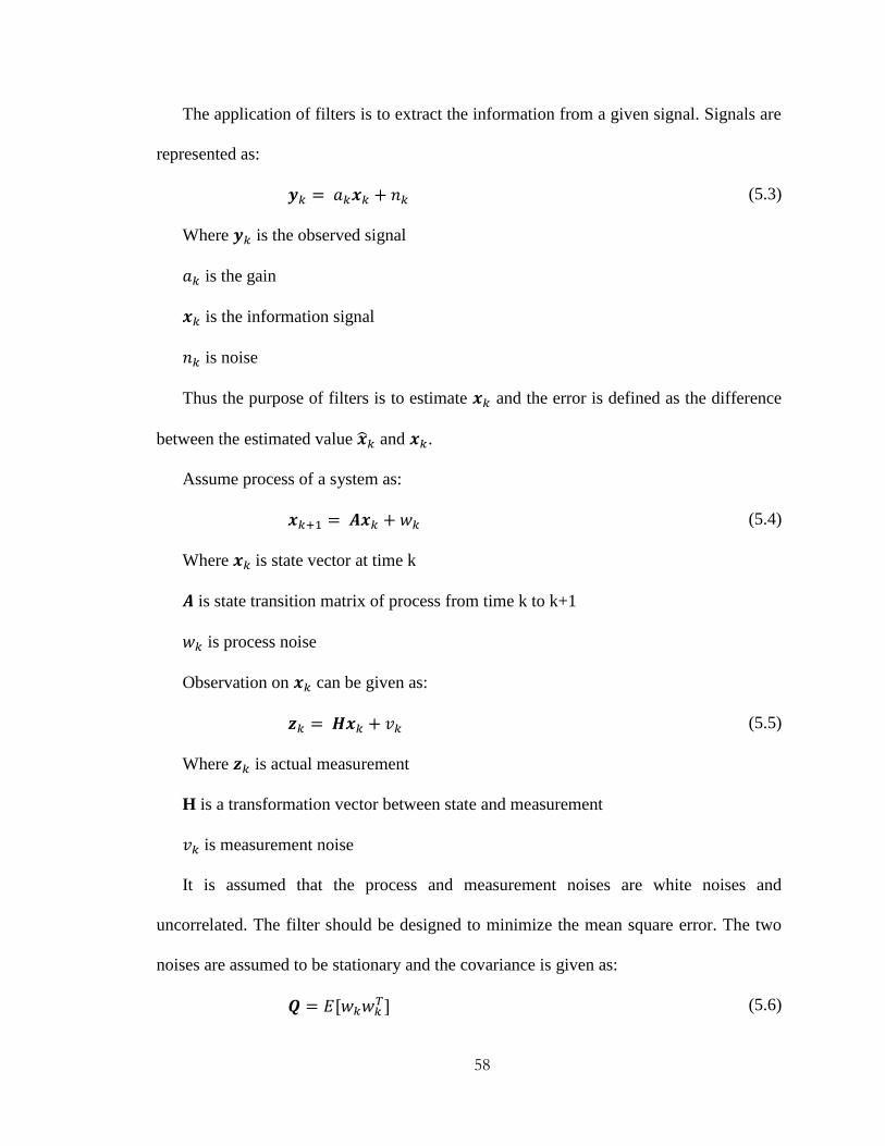
58
The application of filters is to extract the information from a given signal. Signals are
represented as:
(5.3)
Where is the observed signal
is the gain
is the information signal
is noise
Thus the purpose of filters is to estimate and the error is defined as the difference
between the estimated value and .
Assume process of a system as:
(5.4)
Where is state vector at time k
is state transition matrix of process from time k to k+1
is process noise
Observation on can be given as:
(5.5)
Where is actual measurement
H is a transformation vector between state and measurement
is measurement noise
It is assumed that the process and measurement noises are white noises and
uncorrelated. The filter should be designed to minimize the mean square error. The two
noises are assumed to be stationary and the covariance is given as:
(5.6)

59
(5.7)
Mean square error is:
(5.8)
is the error covariance given as:
(5.9)
Where is the estimate of
Let the prior estimate of as . An equation combining measurement with
previous estimated data is given as:
(5.10)
Where is the Kalman gain
is the innovation or measurement module
Substitute Equation (5.5) in Equation (5.10):
(5.11)
Substitute Equation (5.11) in Equation (5.9):
(5.12)
is error of prior estimate and is uncorrelated with measurement noise and
Equation (5.12) is re-written as:
*( )(
) +
(5.13)
Substitute Equation (5.7) and Equation (5.9) in Equation (5.12):
(5.14)

60
Where is prior estimate of
Equation (5.14) is the covariance update equation of Kalman filter. Expanding
Equation (5.14) gives:
(5.15)
Trace of matrix is the same as its transpose, hence:
(5.16)
Where is trace of
Differentiating Equation (5.16) with respect to :
(5.17)
Solving Equation (5.17) by equating it to zero gives:
(5.18)
Thus is derived as:
(5.19)
Equation (5.19) is the Kalman filter equation. The innovation defined in Equation
(5.10) has measurement predicted covariance given as:
(5.20)
Substituting Equation (5.19) in Equation (5.15):
(5.21)
Equation (5.21) is the update equation of error covariance matrix in terms of gain.
Equations (5.10), (5.19) and (5.21) is used in the estimation of . State projection is
calculated from:

61
(5.22)
In recursion process it is important to transfer the error covariance matrix to next time
interval given as:
(5.23)
Extension of Equation (5.9) to time k+1 is:
(5.24)
Errors and are uncorrelated where noise occurs from time k to k+1 and
till time k, hence:
(5.25)
Figure 5-4 shows the technique of Kalman filter design.
Figure 5-4. Kalman filter design
Thus the Kalman filter equations are summarized as the prediction and update
equations [94]. The prediction of the estimate is given as:

62
(5.26)
(5.27)
Where, shows the predicted position of target in the next state
is state transformation matrix
is the observed position of target in the current state
is the predicted covariance
is the covariance of the position of the target
is the covariance of process noise
The update equations of Kalman filter are:
(5.28)
(5.29)
(5.30)
Where, is the Kalman gain
H is the transformation matrix
R is the covariance of measurement noise
is the actual measurement
is the update position of target
is the updated covariance matrix
The – is named as measurement innovation or residual and the Kalman
gain reduces the posteriori error of the filter. The prediction stage predicts the position of
target in the next state and the measurement update equation updates the position based
on , the position of target in the current state. The gain and error estimation covariance

63
becomes stable with time if noise level is assumed to be constant. Noise assumptions play
a very important role in the filter design [95].
The Kalman filter was considered to give the best estimation for linear data. They are
popular due to its optimality, easy implementation and yields good results theoretically
and practically. Kalman filter is used only for linear estimations and not useful in the case
of nonlinear data. Figure 5-5 shows the flow chart of a linear Kalman filter.
Figure 5-5. Kalman Filter Design

64
5.7.1 Implementation of Kalman Filter Tracker Model in radR:
The Kalman filter algorithm is implemented in radR for tracking. The parameters
used and the equations are discussed. Figure 5-6 shows the input given to the Kalman
filter.
Figure 5-6. Input and output parameters for Kalman filter
The dimensions and the noise levels used in the filter design are given in Table 5.1. In
this Kalman design, the input is the x and y position of targets with positive and negative
velocities.
Table 5.1: Input and output parameters for Kalman filter
Kalman Parameters radR Parameters Explanation
* + *
+ is position and is velocity
Acceleration(t) acceleration
0.1*random noise process noise
0.1*random noise measurement noise
Input data obtained from radR for tracking is in the form of data frames. The data
frames store all the target information in the previous frame as old.pts and the current
frame as blips. An example of the data frame is given in Table 5.2. N is the number of
targets in the frame.

65
Table 5.2: Input Data frame of targets in Kalman filter
x y z t ns area int max aspan rspan perim range scan
1
2
.
.
.
N - - . . . . . . . . . . -
The input data frame is read into the Kalman filter algorithm for target tracking. The
estimated target positions of targets are then matched with targets in the current frame.
The Kalman filter as described in the previous section has two stages which are called
prediction and update.
The Kalman filter prediction involves the prediction of target position based on
transition matrices. The transition matrices are time dependent. In this design, the target
position, velocity, acceleration and process noise is used for prediction. The error
covariance and the current measurement are calculated based on the predicted value. The
implementation of equations in the tracker model is given in Equations (5.31), (5.32) and
(5.33). Figure 5-7 shows the two stages in the Kalman filter design.
Figure 5-7. Prediction stage in Kalman filter
Kalman filter equations are described in the previous section [96] and are:
Kalman Filter
Prediction Update Input Output

66
Where the prediction target position and t is the time interval between frames
The noise is assumed as random white noise. radR implementation of Kalman filter
prediction is given as:
The Kalman filter update stage involves computation of Kalman gain and updating of
the target position. Figure 5-8 shows the update stage of the Kalman filter.
Figure 5-8. Update stage of Kalman filter
Kalman Filter
Prediction Update Input Output

67
Kalman filter equations [96] are discussed in details in Section 5.7 and they are
incorporated in the radR as:
The radR implementation of Kalman filter update is given as:
The design of Kalman filter with the association of parameters within the two stages
is shown in Figure 5-9. Implementation of the algorithm is shown in Figure 5-10.
Figure 5-9. Association of parameters within two stages

68
Figure 5-10. Implementation of Kalman filter algorithm in radR
The algorithm is given in the form of a flow chart in Figure 5-11.
Plugins
radR
Tracker Plugin
Tracker Model
Kalman Filter
Input Output
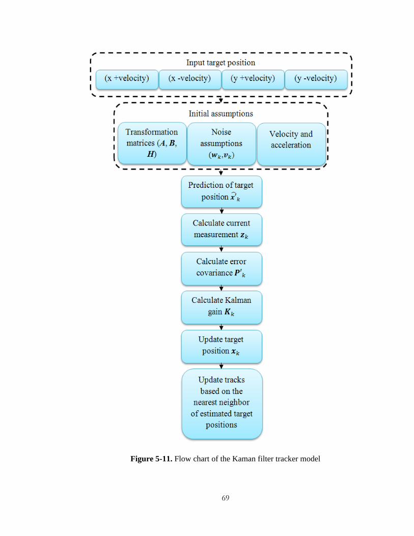
69
Figure 5-11. Flow chart of the Kaman filter tracker model

70
Kalman filter estimates values for each target with positive and negative velocities.
The nearest neighbor data association is applied to match the estimated values with the
targets in the current frame. Figure 5-12 shows the matching of estimated values.
Figure 5-12. Kalman filter design in radR
5.7.2 Variations of Kalman Filter:
Extended Kalman Filter (EKF) is a nonlinear version of the Kalman filter. EKF is a
Kalman filter that linearizes data about the mean and covariance similar to Taylor series
[95]. The system nonlinearities are approximated for the final state estimate using
appropriate linearization of the nonlinear model. Optimal approximation is obtained by
the linearization of the nonlinear model such that it is not affected in any domain [97-99].
In a system with high nonlinearity the EKF gives poor performance and thus
Unscented Kalman Filter (UKF) was developed [100-101]. It is an extended formulation
of unscented transformation. UKF is based on the idea that it is simpler to find
approximation of a probability distribution compared to a nonlinear function.
𝒙𝑘
Kalman filter estimation
Estimated Targets
Actual target position
Data Association
((x - velocity), (y + velocity))
((x -velocity), (y -velocity))
((x+ velocity), (y + velocity))
((x+ velocity), (y - velocity))

71
The UKF gives greater performance during high non linearity as the Gaussian random
variable is given as a number of points which obtains the mean and covariance of the
system with higher accuracy. The UKF can be used if EKF gives poor performance, for
all other cases EKF is a better option because of its low computation cost. The
performance of the EKF greatly depends on the accuracy of data linearization. However
the performance of UKF was found to be better than particle filters [102]. Kalman-Bucy
is the continuous time version of discrete Kalman filter and has been described in
Reference [103].
Ensemble Kalman Filter (EnKF) design uses an ensemble which is samples for a state
to create an analysis phase for the system. The analysis uses the same Kalman gain value
and hence reduces the computational cost. EnKF can be implemented only if the
ensemble of a system can be represented statistically. The size assumption of the
ensemble is also important as small sizes gives rise to under sampling [104]. The
ensemble Kalman filter is very efficient because of the low dimensions of matrices used.
These filters are divided into two and are called as perturbed observations and square root
filter [105].
5.8 Particle Filter
Tracking for nonlinear and non-Gaussian data can be performed by particle filter as
Kalman filter assumes data as Gaussian. In the presence of multiple targets within single
radar beam tracking becomes difficult as the discrimination of target is inaccurate.
Particle filters are used in this case by calculating the posterior density for different
values of targets which is converted to likelihood functions and helps to detect the
number of targets. This approach can simultaneously handle processing, data association

72
and tracking targets [108-110]. Particle filters are also known as sequential Monte Carlo
filters and are used when the system is nonlinear and non-Gaussian. Particles filters are a
version of point mass filters in which the particles are present in the place of higher
probability of occurrence. If for the Bayesian models in the design the integrals cannot be
analyzed then the posterior pdf can be represented as a set of randomly defined weights
[108-110]. Sequential importance filtering is a simple particle filter estimation method. In
this a recursively occurring Bayesian filter technique is used. The posterior density is
calculated as weights. The output is in the form of samples and their corresponding
weights.
5.8.1 Sequential Importance Sampling (SIS):
In this method the posterior density is defined as a set of samples with weights. Let
the initial position of the targets with their associated weights be
is a
user defined parameter which represents the number of particles. The posterior density
can be approximated as:
∑
(5.41)
is a set of all states up to time k
is the number of measurements available up to time k
Weights are assigned based on the concept of important sampling. Consider a system
with probability density which cannot be calculated appropriately. Let this
probability density be proportional to a value which is easy to analyze. The samples
for points are evaluated from importance density represented as Weight is
calculated as
and the weighted approximation for density is:

73
∑
(5.42)
If are derived from importance density then weights are defined as:
(
( )
) (5.43)
The weights are updated with the Equation (5.44):
( ( |
)
)
(5.44)
The filtered posterior density is given as:
∑
(5.45)
Figure 5-13 shows the algorithm of SIS particle filters in which number of particles
are assumed. The particles are initialized with posterior density and weights. The weights
of the particles are updated and they define the probability of occurrence of the particle in
the new state [109].

74
Figure 5-13. Sequential Importance Sampling Particle Filter
5.8.2 Implementation of Particle Filter Tracker Model in radR:
The particle filter algorithm is implemented in radR for tracking. Figure 5-14 shows
the structure of the particle filter.
Figure 5-14. Input and output parameters for the particle filter
The input and output parameters used in this design are given in Table 5.3.

75
Table 5.3: Input and output parameters for particle filter
Particle Filter
Parameters
radR Parameters Explanation
is the number of particles assumed
Number of particles around the initial
target position
Random weights with range (0:1)
∑
Posterior density is the summation of
product of updated weights and
predicted values for the particles.
Input data obtained from radR for tracking is in the form of data frames. The data
frames store all the target information in the previous frame as old.pts and the current
frame as blips. An example of the data frame is given in Table 5.4. N is the number of
targets in the frame.
Table 5.4: Input Data frame of targets in particle filter
x y z t ns area int max aspan rspan perim range scan
1
2
.
.
.
N - - . . . . . . . . . . -
The input data frame is read and the particle filter algorithm is computed for tracking
the targets. The estimated target positions of targets are then matched with targets in the
current frame. The particle filter as described in the previous section first initializes a
nonlinear system prediction for assumed number of particles and then their weights are

76
updated. The prediction for the particles is the initial part of the design. Figure 5-15
shows the two stages of the design.
Figure 5-15. Prediction for N particles
The initial stage involves prediction of values ( |
) and ( | ). Consider a
nonlinear system as:
Where is the input target position
and are the process and measurement noise
and are nonlinear functions of process and observation vector
is the current observed measurement
Equations (5.46) and (5.47) are used to predict the values of the system. Equations for
particle filter can be assumed as:
Particle Filter
Prediction for
N Particles Update
Input Output

77
h = 0.96
Equations (5.48) and (5.49) are implemented for Ns number of particles as:
The prediction is performed for both positive and negative velocity of targets in the
particle filter model. Weights are updated and the posterior density is calculated. Figure
5-16 shows the update part of the particle filter.
Figure 5-16. Update in particle filter
The weight update and posterior density is calculated as:
Implemented weight update and posterior density calculation in radR are:
Particle Filter
Prediction
for Ns
Particles
Update
weights and
posterior
density
Input Output

78
The posterior density is the estimated value of the target. The association of parameters
within the two stages is shown in Figure 5-17. Implementation of the algorithm is shown
in Figure 5-18.
Figure 5-17. Association of parameters within two stages
Figure 5-18. Implementation of Particle filter algorithm in radR
A flow chart of the particle filter algorithm is shown in Figure 5-19.
Plugins
radR
Tracker Plugin
Tracker Model
Particle Filter
Input Output

79
Figure 5-19. Flow chart of the particle filter tracker model

80
Particle filter estimates values for each target with positive and negative velocities.
The nearest neighbor data association is applied to match the estimated values with the
targets in the current frame. Figure 5-20 shows the matching of estimated values.
Figure 5-20. Particle filter design in radR
5.9 Compressive Sampling:
Data occurring in real time are generally sparse but most of the signal processing
methods ignores this fact. Compressive Sampling is based on the idea that for certain
signals a small number of samples within the signal are enough to represent the entire
signal. The signal reconstruction is based on how accurate the signal is approximated
from the available samples [111-113].
Consider vectors which has (quasinorm) defined as:
The signal x is sparse if ||x||o<=s, where s defines the sparsity of the signal. Sparsity
means non zero values in the signal. Sample is a function of the given signal. Many
𝒙𝑘
Particle filter estimation
Estimated Targets
Actual target position
Data Association
((x - velocity), (y + velocity))
((x -velocity), (y -velocity))
((x+ velocity), (y + velocity))
((x+ velocity), (y - velocity))

81
samples can be extracted for the signal and is called a sampling matrix ( ). Consider for
the given signal , m samples are extracted. The sampling matrix has (m, N)
dimensions. It is important to identify the measurements required to attain sparse signals.
Two dissimilar sparse signals should not be mapped to the same samples and Restricted
Isometry Property (RIP) is applied to preserve sparsity [111].
Restricted Isometry Property (RIP) helps in characterizing a matrix which contains
sparse vectors. Consider an observed signal represented as:
(5.57)
Where is the signal to be recovered
is observations at current state
is a matrix of dimensions
In sparse signals if , has to be reconstructed with good approximation. To
reconstruct accurately it should be a sparse signal and the known matrix should
satisfy the RIP. The Restricted Isometry Property (RIP) of is given as:
‖ ‖ ‖ ‖
‖ ‖ (5.58)
Where is the sampling matrix which is a linear function of the data.
is the least number of the sampling matrix which satisfies the RIP property [114].
Signal recovery algorithms are used to reconstruct a signal from a vector which
contains noisy data. A greedy pursuit algorithm can be used for signal reconstruction.
In greedy pursuits, approximations are based on a step by step process until an
optimal condition is reached. In these methods a signal is recovered recursively and
reconstructed using pseudo inverse. Some of the greedy methods are Orthogonal

82
Matching Pursuit (OMP), stage wise OMP (StOMP) and Regularized OMP (ROMP)
[115].
5.9.1 CoSaMP:
Compressive Sampling Matching Pursuit (CoSaMP) is a greedy pursuit method for
signal reconstruction [112-113]. Let be a sampling matrix of dimensions which
has a restricted isometry property The signal is a set of vectors given as ,
where e is noise. For precision given by parameter the CoSaMP gives an
approximation a that satisfies:
‖ ‖
√ ‖ ‖
‖ ‖ (5.59)
Where is the (s/2 ) – sparse approximation of x
is the precision parameter
e is the noise
a is the sparse approximation selected to satisfy the condition
Sparse approximation can be selected in two ways, one is by
where m is
the number of measurements of a signal of length N and another method is to vary the
range of values and select the best fit as the sparse level.
In CoSaMP the most important steps are:
Identification of largest components of the signal
Merging the identified values with the current approximation
Estimation using least squares method
Retaining only the largest components from the least square
Update the procedure till the required residue is obtained [111]

83
5.10 BCoSaMP:
Most signals obtained at real time are sparse. Signals are sampled through
compression techniques using linear projection of signal and a projection matrix is
formed. The Compressive Sampling Matching Pursuit algorithm (CoSaMP) is a greedy
approach and the state error decreases over the number of iterations [116].
BCoSaMP (Block CoSaMP) divides the projection matrix into grids. They are created
by the Doppler-delay plane given as (delay factor) and (Doppler factor). Target
tracking is based on grids. If the number of targets present is less than the Doppler-delay
plane then it is a sparse target data. If P is the position of target travelling with a velocity
v with the direction of arrival is then the delay and Doppler factor is given as:
(5.60)
⟨ ⟩
(5.61)
Where is the delay factor
is the position of target
is the speed of light in meters per second
is the Doppler factor
is the velocity of target
is the direction of arrival of the target
The predicted value of the target is given as:
*
+ (5.62)
Where is the predicted value
is the current value

84
is the noise level
The sparse model is created using the delay and Doppler grid which is given
as Consider M targets in these grid points then the measurement model at k
is given as:
∑∑
(
)
(5.63)
Where ∑ ∑
(
) is a sampling matrix which has the delay-Doppler factors of
targets within the grid
is the noise
Equation (5.63) can be modified as:
(5.64)
Where, is called the sampling matrix and *
(
)+
is the noise
Thus each block gives the sampling matrix of delay Doppler grid of the target. This is the
method of creating a block sparse signal for the given data to which the CoSaMP
algorithm is applied for tracking.
5.10.1 Algorithm:
Step 1: is the predicted value given in Equation (5.62)
Step 2: The residue is given as r = which is the current measurement
Step 3: Create state proxy p =
Here φ is the sampling matrix with φ =
This consists of all possible combinations of delay and Doppler factor.

85
Step 4: Ω = bsupp( )
Where bsupp is called block support which indicates non-zero block values
The largest blocks of the matrix are identified and if the number of targets is less than the
grid size, assume s = m where m is the number of targets
Choose the highest 2s block from the matrix as Ω, where s is the sparsity level
Step 5: T = Ω U bsupp( )
Merge the block supports with the predicted value
Step 6: = , is the state estimation using least squares
Step 7: Estimated value
=
Step 8: Residue
r = -
Step 9: Continue steps 3 to 8 till the required halting criteria of the residue is reached.
Step 10: Estimated value at the final stage is the target position at current state.
Residue r increases in the beginning and then it decreases at a certain point. This point
will be used as a termination criterion and program will be stopped [117]. Figure 5-21
shows the BCoSaMP algorithm.

86
Figure 5-21. Flowchart of BCoSaMP algorithm
5.10.2 Implementation of BCoSaMP Tracker Model in radR:
The BCoSaMP algorithm is implemented in radR for tracking. Figure 5-22 shows
various input given to the BCoSaMP algorithm.
Initializations:
Sparse Level S
System matrix
Current Measurement
Create State proxy
Select the blocks that have
high S levels and merge
State estimation based on
least squares method
Calculate residue
Until halting
criteria
Final estimated value
No
Yes

87
Figure 5-22. Input and output parameters for BCoSaMP
The input parameters used in the design are given in Table 5.5. The grid size is
defined based on many trials and choosing the size with the least error rate.
Table 5.5: Input and output parameters for BCoSaMP
BCoSaMP
Parameters
radR Parameters Explanation
Initial target position in terms of
Doppler factors
=(60* ) X (40* ) Grid in terms of range and time delay
S
S= number of targets within
grid
Number of targets within the grid
Sampling matrix consisting of
Doppler factors for the entire grid
Input data obtained from radR for tracking is in the form of data frames. The data
frames store all the target information in the previous frame as old.pts and the current
frame as blips. An example of the data frame is given in Table 5.6.
Table 5.6: Input Data frame of targets in BCoSaMP
x y z t ns area int max aspan rspan perim range scan
1
2
.
.
N . . . . . . . -

88
The input data frame is read and the BCoSaMP algorithm is implemented for the
targets. The estimated target positions of targets are then matched with targets in the
current frame.
The prediction of position of target is calculated similar to Kalman filter. Figure 5-23
shows the two stages of the design.
Figure 5-23. Prediction of target position
The prediction of target position is calculated using the formula:
where t is the sampling interval. t=0.8 is used for three nautical mile range for the
marine radar.
Implementation of target prediction in radR model:
The next stage involves the update of the target position. Figure 5-24 shows the
update stage of BCoSaMP.
BCoSaMP
Prediction Update Input Output
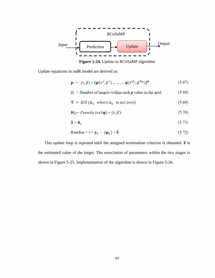
89
Figure 5-24. Update in BCoSaMP algorithm
Update equations in radR model are derived as:
This update loop is repeated until the assigned termination criterion is obtained. is
the estimated value of the target. The association of parameters within the two stages is
shown in Figure 5-25. Implementation of the algorithm is shown in Figure 5-26.
BCoSaMP
Prediction Update Input Output

90
Figure 5-25. Association of parameters within two stages
Figure 5-26. Implementation of BCoSaMP algorithm in radR
The algorithm is given in the form of a flow chart in Figure 5-27.
Plugins
radR
Tracker Plugin
Tracker Model
BCoSaMP
Input Output

91
Figure 5-27. Flow chart of BCoSaMP model
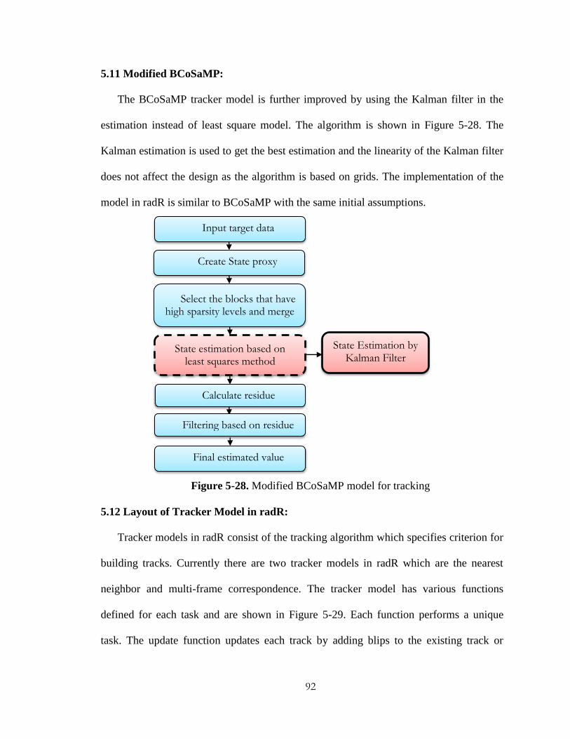
92
5.11 Modified BCoSaMP:
The BCoSaMP tracker model is further improved by using the Kalman filter in the
estimation instead of least square model. The algorithm is shown in Figure 5-28. The
Kalman estimation is used to get the best estimation and the linearity of the Kalman filter
does not affect the design as the algorithm is based on grids. The implementation of the
model in radR is similar to BCoSaMP with the same initial assumptions.
Figure 5-28. Modified BCoSaMP model for tracking
5.12 Layout of Tracker Model in radR:
Tracker models in radR consist of the tracking algorithm which specifies criterion for
building tracks. Currently there are two tracker models in radR which are the nearest
neighbor and multi-frame correspondence. The tracker model has various functions
defined for each task and are shown in Figure 5-29. Each function performs a unique
task. The update function updates each track by adding blips to the existing track or
Create State proxy
Select the blocks that have high sparsity levels and merge
State estimation based on least squares method
Calculate residue
Final estimated value
Input target data
State Estimation by Kalman Filter
Filtering based on residue

93
starting a new track. Other functions are used to define the maximum speed of the track,
select, deselect, load and unload a model. Get Menu function receives the user input for
controlling the tracking procedure based on the minimum number of blips required to
form a track and its maximum speed. Set blip fresh time selects the expiry time of the
track. If the player is stopped or paused the scans are reprocessed. The tracking algorithm
is implemented inside the update function. Gain array is created which stores the column
index of the matched blips. Details of two current tracker models in radR are discussed
in Chapter 4.
Figure 5-29. Algorithm for tracker model
5.12.1 Update Function:
The tracking algorithm is implemented inside the update function. Tracking algorithm
identifies appropriate tracks for each blip. Tracks are stored in a file called
Get menu function
Select function
Deselect function
Load function
Unload function
Set blip fresh time function
Set track stale time function
Update function Adds blips to tracks
Assign parameters for track
Track onset
Track expiry
Load a plugin
Unload a plugin
Active blip time
Active track time
Tracking algorithm

94
which_slots_full. Tail points of each track are saved in old.pts data frame and current
blips are available in blips data frame. Blip information is extracted from these data
frames using blips$parameter (e.g. blips$x for x-position) or old.pts$parameter. Tracking
algorithm builds tracks by matching each blip in the current frame to the active tracks.
Blips which have no matches start new tracks. Gain array is defined in this function
which stores the index of the matched blips. The blips which have no matches are
retained for three consecutive scans and are then terminated. Gain array obtained from
the tracker model file is used by tracker plugin to create tracks on the GUI. Figure 5-30
shows the layout of tracker model in radR.
Figure 5-30. Layout of tracker model in radR
5.13 Development of Tracker Models:
Four models were implemented in radR for tracking and are discussed in detail in the
following sections. Four tracking algorithms implemented in this work are Kalman filter,
particle filter, Block Compressive Sampling Matching Pursuit (BCoSaMP) and modified
Scan (t-1) Scan (t)
Tracker Plugin
old.pts blips
Tracking Algorithm
Matched blips
Saves & plots
tracks
Model for
building tracks

95
BCoSaMP. Figure 5-31 shows four tracker models developed in radR for different data
types.
Figure 5-31. Developed tracker models in radR
The nearest neighbor model is used as a template. The tracking algorithm is
implemented in the update function. Figure 6-4 shows the layout of the tracker model and
the existing tracking algorithm (Nearest Neighbor) is replaced by one of the newer
tracking algorithms as shown in Figure 5-32. Tracker models can then be created in radR.
Figure 5-32. Implementation of new algorithms in radR
Scan (t-1) Scan (t)
Tracker Plugin
old.pts blips
Tracking Algorithm
Matched blips
Implementation
of new
algorithms
Data
Linear & Gaussian
Non Linear & Non
Gaussian
Sparse data with least
square
Sparse data with Kalman
filter
Kalman Filter Particle Filter BCoSaMP Modified BCoSaMP

96
5.13.1 Kalman Filter Tracker Model:
The Kalman filter was discussed in Chapter 5. A linear discrete Kalman filter model
is used for tracking. Important steps in Kalman filter implementation are input target
location, initial assumptions, prediction stage, update stage and data association. Many
trials are made to make sure that the assumptions are appropriate for the environmental
conditions and the amount of noise levels in the data.
Steps for Kalman filter design includes the creation of file kalman.model.R in the
tracker plugin folder. The Kalman filter tracking algorithm is implemented inside the
update function. Input is taken as the data from the previous frame and is defined as
old.pts in radR. Gaussian noise has been assumed. The velocity of the bird target is set to
8 m/sec. The velocity can be varied based on wind conditions. The prediction and update
operations of Kalman filter provide the final estimation for each target. In multiple target
environment, there is a possibility of appearance of noise along with accurate bird tracks.
Estimated values are matched to the blips in the current frame based on the minimum
distance. Since the nearest neighbor technique is used for data association, every point
has a track and this inefficiency can be removed by setting a threshold value for the
distance. A gain function is created similar to the nearest neighbor tracker model in radR
and hence the tracks are updated according to the Kalman filter algorithm.
In this tracker model design, target with positive and negative velocities are assumed
to find appropriate tracking in all directions irrespective of the target’s motion. Various
steps of the Kalman filter design are shown in Figure 5-33. Outlines of nearest neighbor,
multi-frame and Kalman filter are also shown in Figure 5-33.

97
Figure 5-33. Comparison of current tracker models with Kalman filter
Multi-frame
Gain array with matched blips
Tracker plugin
Initial target
position
Positive and
negative
velocity
assumption
Noise
assumptions
Initialization of
transition
matrices
Target
prediction
Covariance
prediction,
Kalman gain
Update target
position
Nearest
neighbor data
association
Set max. distance,
max. speed, min.
gain
Gain calculation
Velocity
filtering
Set gain below
threshold to
zero
Set gain above
threshold to one
Target
prediction
Point to point
gain calculation
Save
correction and
extension
edges between
frames
Calculate gain
for additional
points in new
frame
Save max. path
cover
Track to point
gain calculation
Distance
between blips
in two frames
Gain
calculation
Velocity
filtering
Change in rate
of intensity
filtering
Change in rate
of area filtering
Change in rate
of turning
angle filtering
Bipartite
matching to
form tracks
Kalman filter Nearest Neighbor

98
5.13.2 Particle Filter Tracker Model:
The particle filter is implemented inside the update function. The implementation of
the model is similar to the Kalman filter tracker model. Initial parameters for particle
filter are the number of particles, weight assignment for each particle, the target initial
position, the nonlinearity of data and the assigned probability of detection based on
weight levels.
Steps for particle filter design include the creation of particle.model.R file in the
tracker plugin folder. The basic model of Sequential Importance Sampling (SIS) particle
filter is considered in this work with 100 particles. Initializations include input data which
is the position of targets, number of particles, pdf of each particle in the form of weights.
Second stage includes the filter design for N number of particles. Weights are
updated for each particle. The pdf is calculated to update the target position. Thus
estimates for the targets are obtained. The data association is the final stage of the design
and the nearest neighbor technique is used. A gain function is created with the matched
blips for tracking. To overcome the limitation of missed target detection, blips in the
frame are retained for at least three frames in the future scans. Comparison of current
tracker models with particle filter is given Figure 5-34.

99
Figure 5-34. Comparison of current tracker models with particle filter
Multi-frame
Gain array with matched blips
Tracker plugin
Initial target
position
Number of
particles and
weights
assigned
Target
prediction
Update the
weights
Update target
position
Nearest
neighbor data
association
Set max. distance,
max. speed, min.
gain
Gain calculation
Velocity
filtering
Set gain below
threshold to
zero
Set gain above
threshold to one
Target
prediction
Point to point
gain calculation
Save
correction and
extension
edges between
frames
Calculate gain
for additional
points in new
frame
Save max. path
cover
Track to point
gain calculation
Distance
between blips
in two frames
Gain
calculation
Velocity
filtering
Change in rate
of intensity
filtering
Change in rate
of area filtering
Change in rate
of turning
angle filtering
Bipartite
matching to
form tracks
Particle filter Nearest Neighbor

100
5.13.3 BCoSaMP Tracker Model:
The block compressive sampling matching pursuit algorithm is used for tracking
based on the sparse techniques. The algorithm is modified for the marine radar data as the
radar is assumed to be stationary in this work. The model is implemented inside the
update function in filename.model.R file. The data is assumed to be sparse. In case of
real time data, it is important to assign an appropriate residue function to avoid an infinite
loop.
Steps for BCoSaMP filter design include the creation of bcosamp.model.R file in the
tracker plugin folder. Initial steps required for this algorithm are conversion of the target
position, direction of arrival or bearing and velocity to Doppler models. The sampling
interval is selected based on the data range for prediction of target position. The grid size
is defined around the target based on the predicted value. The sparse level is defined
based on the number of targets present within the assigned grid. A sampling matrix
containing the Doppler factors for the defined grid is created. The second part of the filter
design includes formation of state proxy using the sampling matrix, identifying the
largest sparse blocks and merging with the predicted value.
The update stage is the least square estimation of the blocks. The residue is calculated
for the value obtained and the loop is stopped when the required termination criteria is
reached. The value of position is updated when the loop terminates giving the estimated
target position. Final estimated values are then converted back to Cartesian form and the
nearest neighbor data association is performed. A threshold is applied for each estimated
value based on the value of residue. Comparison of current tracker models with
BCoSaMP Algorithm is given in Figure 5-35.

101
Figure 5-35. Comparison of current tracker models with BCoSaMP Algorithm
Multi-frame
Gain array with matched blips
Tracker plugin
Initial target
position
Conversion of
position to
Doppler
factors
Define Sparsity
level
Assume grid
size and create
sampling
matrix
Least square
estimation
Nearest
neighbor data
association
Set max. distance,
max. speed, min.
gain
Gain calculation
Velocity
filtering
Set gain below
threshold to
zero
Set gain above
threshold to one
Target
prediction
Point to point
gain calculation
Save
correction and
extension
edges between
frames
Calculate gain
for additional
points in new
frame
Save max. path
cover
Track to point
gain calculation
Distance
between blips
in two frames
Gain
calculation
Velocity
filtering
Change in rate
of intensity
filtering
Change in rate
of area filtering
Change in rate
of turning
angle filtering
Bipartite
matching to
form tracks
BCoSaMP Nearest Neighbor
Residue
calculation

102
5.13.4 Modified BCoSaMP Tracker Model:
The modified BCoSaMP model is created similar to the BCoSaMP model with the
same assumptions. The least square estimation is replaced with Kalman filter estimation
for the model.
Figure 5-36 shows various models developed in radR environment and results are
discussed in the following sections.
Figure 5-36. New tracker models in radR
5.14 Summary:
Four tracker models are discussed and they have been implemented in radR. Four
tracker algorithms are Kalman filter, particle filter, BCoSaMP and modified BoCoSaMP.
Tracker algorithms incorporate various parameters and various assumptions are
described. Compressive Sampling Matching Pursuit (CoSaMP) is used for reconstruction

103
of sparse signals. It is proved to be robust and efficient method for signal recovery. This
technique is used for efficiently tracking multiple targets and its efficiency is proved to be
better than or equal to particle filter with less computation time [117]. The study area and
results with various types of data are discussed in the following chapter.
104
Chapter 6
Simulation and Results
6.1 Introduction:
Ottawa National Wildlife Refuge, OH was recommended as the study site by the
project team’s wildlife biologists. This wildlife refuge was established in 1961 to serve as
a habitat for migrating birds. The habitat at Ottawa Wildlife Refuge is protected to offer
nesting and stopover opportunities during migration period and habitat for birds [118].
The radar was set up at the location shown in Figure 6-1 along the coastline of western
Lake Erie basin to study behavior of birds. The marine radar was run all through the night
and the data was analyzed to study behavior of nocturnal migrating birds during the fall
and spring migration period.

105
Figure 6-1. Study area- Ottawa National Wildlife Refugee
Courtesy: Google Earth
Four tracking algorithms have been considered in this work and have been
implemented within radR. Performance of these implemented tracking algorithms is
evaluated and compared with currently available Multi-frame tracker model in radR and
is discussed in the following sections.
6.2 Radar Data:
The output of the tracking algorithms are analyzed with three types of data set. Single
simulated track at constant velocity of 8 m/sec for 25 scans. Figure 6-2 shows the
simulated track. Four simulated tracks occurring simultaneously for 25 scans in radR.
The four tracks are simulated in the radR and the graphical representation of the tracks is
shown in Figure 6-3.

106
Figure 6-2. Single simulated track at constant velocity
Figure 6-3. Simulated multi-target tracks

107
Figure 6-4 shows the tracks simulated with the enabling of target trails plugin.
Figure 6-4. Simulated multi-target tracks in radR environment
Marine radar data collected at the Ottawa National Wildlife Refuge on April 20, 2012
using T-bar antenna in the vertical mode from 4:13 AM to 6:45 AM was also used.
Various tracking algorithms are tested with different data sets and their performance is
analyzed. Snapshot of marine radar data is shown in Figure 6-5.

108
Figure 6-5. Snapshot of marine radar data
6.3 Simulations of Tracker Models:
Kalman filter tracking algorithm was tested with previously described simulated
tracks. Figure 6-6 shows the output of the Kalman filter tracking with the actual target
track. The error rate of the Kalman filter is shown in Figure 6-7. Kalman filter in case of
a single track estimates the target position with very less error rate. It can also be seen
that the error is decreasing with the increase in time.

109
Figure 6-6. Kalman filter single target tracking
Figure 6-7. Error rate of Kalman filter
0 5 10 15 20 250
0.5
1
1.5
2
2.5
3
3.5
4
4.5Kalman Filter Error
Number of scans
Err
or
(perc
enta
ge)

110
Figure 6-8 shows the output of the Kalman filter tracking with four target tracks. The
error rate of the Kalman filter is shown in Figure 6-9. It can also be seen that the error is
decreasing with the increase in time.
Figure 6-8. Multi target tracking using Kalman filter
Figure 6-9. Error rates for the four tracks
-800 -600 -400 -200 0 200 400 600 800-800
-600
-400
-200
0
200
400
600
800
1000
x coordinate (meters)
y co
ordi
nate
(m
eter
s)
Kalman Tracking
Simulated Data
Kalman Output
0 5 10 15 20 250
2
4
6
8
10
12
Number of scans
Err
or (
perc
enta
ge)
Kalman Filter Error
Track 1
Track 2
Track 3
Track 4
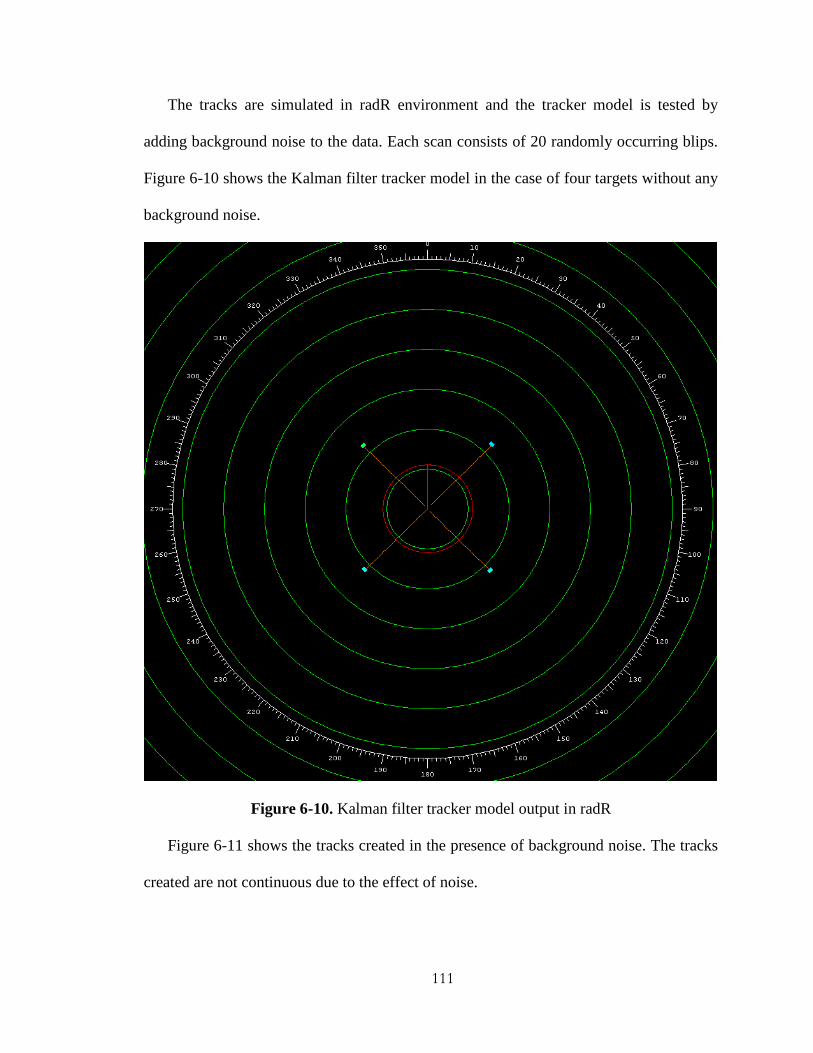
111
The tracks are simulated in radR environment and the tracker model is tested by
adding background noise to the data. Each scan consists of 20 randomly occurring blips.
Figure 6-10 shows the Kalman filter tracker model in the case of four targets without any
background noise.
Figure 6-10. Kalman filter tracker model output in radR
Figure 6-11 shows the tracks created in the presence of background noise. The tracks
created are not continuous due to the effect of noise.

112
Figure 6-11. Kalman filter tracker model output with noise in radR
Figure 6-12 shows the output of the particle filter tracking with the actual target track.
Figure 6-13 shows the error rate of particle filter estimated target track. Particle filter
in case of a single track estimates the target position more accurately than Kalman filter
model.
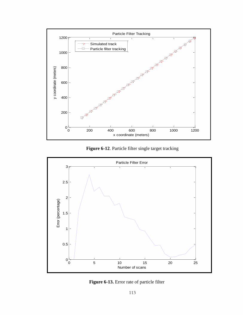
113
Figure 6-12. Particle filter single target tracking
Figure 6-13. Error rate of particle filter
0 200 400 600 800 1000 12000
200
400
600
800
1000
1200Particle Filter Tracking
x coordinate (meters)
y c
oord
inate
(m
ete
rs)
Simulated track
Particle filter tracking
0 5 10 15 20 250
0.5
1
1.5
2
2.5
3Particle Filter Error
Number of scans
Err
or
(perc
enta
ge)

114
Figure 6-14 shows the Particle filter estimated track for multi targets. Figure 6-15
gives the error rate of the four tracks.
Figure 6-14. Multi target tracking using particle filter
Figure 6-15. Error rates for the four tracks
-800 -600 -400 -200 0 200 400 600 800-800
-600
-400
-200
0
200
400
600
800
1000
x coordinate (meters)
y co
ordi
nate
(m
eter
s)Particle Filter Tracking
Simulated tracks
Particle filter tracking
0 5 10 15 20 250
2
4
6
8
10
12
14
Number of scans
Err
or (
perc
enta
ge)
Particle Filter Error
Track 1
Track 2
Track 3
Track 4

115
The tracks are simulated in radR environment and the tracker model is tested by
adding background noise to the data. Each scan consists of 20 randomly occurring blips.
Figure 6-16 shows the particle filter tracker model output in the case of four targets
without any background noise.
Figure 6-16. Particle filter tracker model output in radR
Figure 6-17 shows the tracks created in the presence of background noise. The tracks
created are not continuous due to the effect of noise.

116
Figure 6-17. Particle filter tracker model output with noise in radR
The BCoSaMP estimation of the target is shown in Figure 6-18. Figure 6-19 shows
the error rate of the estimated track.
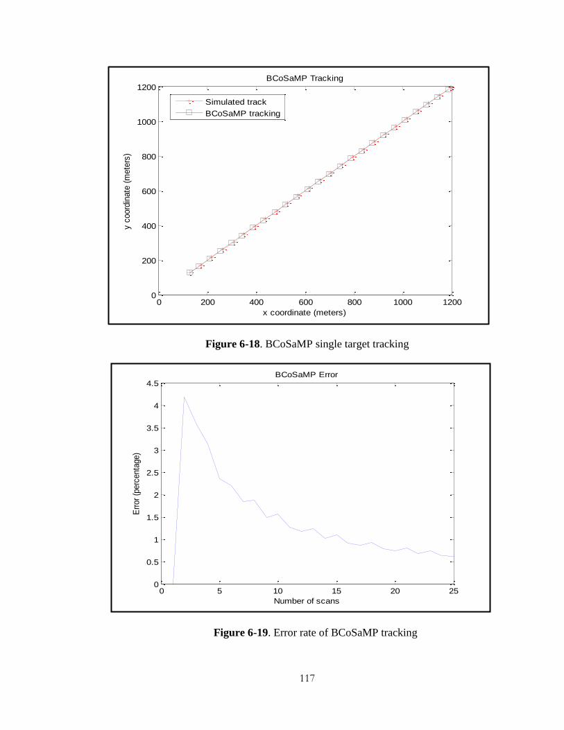
117
Figure 6-18. BCoSaMP single target tracking
Figure 6-19. Error rate of BCoSaMP tracking
0 200 400 600 800 1000 12000
200
400
600
800
1000
1200
x coordinate (meters)
y c
oord
inate
(m
ete
rs)
BCoSaMP Tracking
Simulated track
BCoSaMP tracking
0 5 10 15 20 250
0.5
1
1.5
2
2.5
3
3.5
4
4.5BCoSaMP Error
Number of scans
Err
or
(perc
enta
ge)

118
Figure 6-20 shows the BCoSaMP estimated track for multi targets. Figure 6-21 gives
the error rate of the four tracks.
Figure 6-20. Multi target tracking using BCoSaMP
Figure 6-21. Error rates for the four tracks
-800 -600 -400 -200 0 200 400 600 800-800
-600
-400
-200
0
200
400
600
800
x coordinate (meters)
y co
ordi
nate
(m
eter
s)BCoSaMP Tracking
Simulated tracks
BCoSaMP tracking
0 5 10 15 20 250
1
2
3
4
5
6
7
8
9
Number of scans
Err
or (
perc
enta
ge)
BCoSaMP Error
Track 1
Track 2
Track 3
Track 4
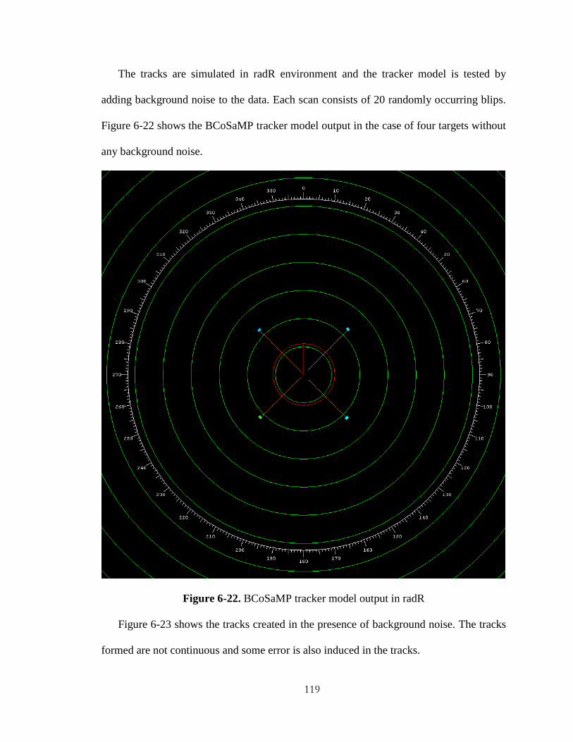
119
The tracks are simulated in radR environment and the tracker model is tested by
adding background noise to the data. Each scan consists of 20 randomly occurring blips.
Figure 6-22 shows the BCoSaMP tracker model output in the case of four targets without
any background noise.
Figure 6-22. BCoSaMP tracker model output in radR
Figure 6-23 shows the tracks created in the presence of background noise. The tracks
formed are not continuous and some error is also induced in the tracks.

120
Figure 6-23. BCoSaMP tracker model output with noise in radR
The modified BCoSaMP estimation of the target is shown in Figure 6-24. Figure 6-25
shows the error rate of the estimated track.

121
Figure 6-24. Modified BCoSaMP single target tracking
Figure 6-25. Error rate of modified BCoSaMP tracking
0 200 400 600 800 1000 12000
200
400
600
800
1000
1200
x coordinate (meters)
y c
oord
inate
(m
ete
rs)
Modified BCoSaMP Tracking
Simulated Track
Modified BCoSaMP
0 5 10 15 20 250
0.1
0.2
0.3
0.4
0.5
0.6
0.7
0.8Modified BCoSaMP Error
Number of Scans
Err
or
(perc
enta
ge)

122
Figure 6-26 shows the BCoSaMP estimated track for multi targets. Figure 6-27 gives
the error rate of the four tracks.
Figure 6-26. Multi target tracking using modified BCoSaMP
Figure 6-27. Error rates for the four tracks
0 5 10 15 20 250
1
2
3
4
5
6
7
8
9
Number of scans
Err
or (
perc
enta
ge)
Modified BCoSaMP Error Rate
Track 1
Track 2
Track 3
Track 4
-800 -600 -400 -200 0 200 400 600 800-800
-600
-400
-200
0
200
400
600
800
x coordinate (meters)
y co
ordi
nate
(m
eter
s)Modified BCoSaMP Tracking
Simulated track
Modified BCoSaMP tracking
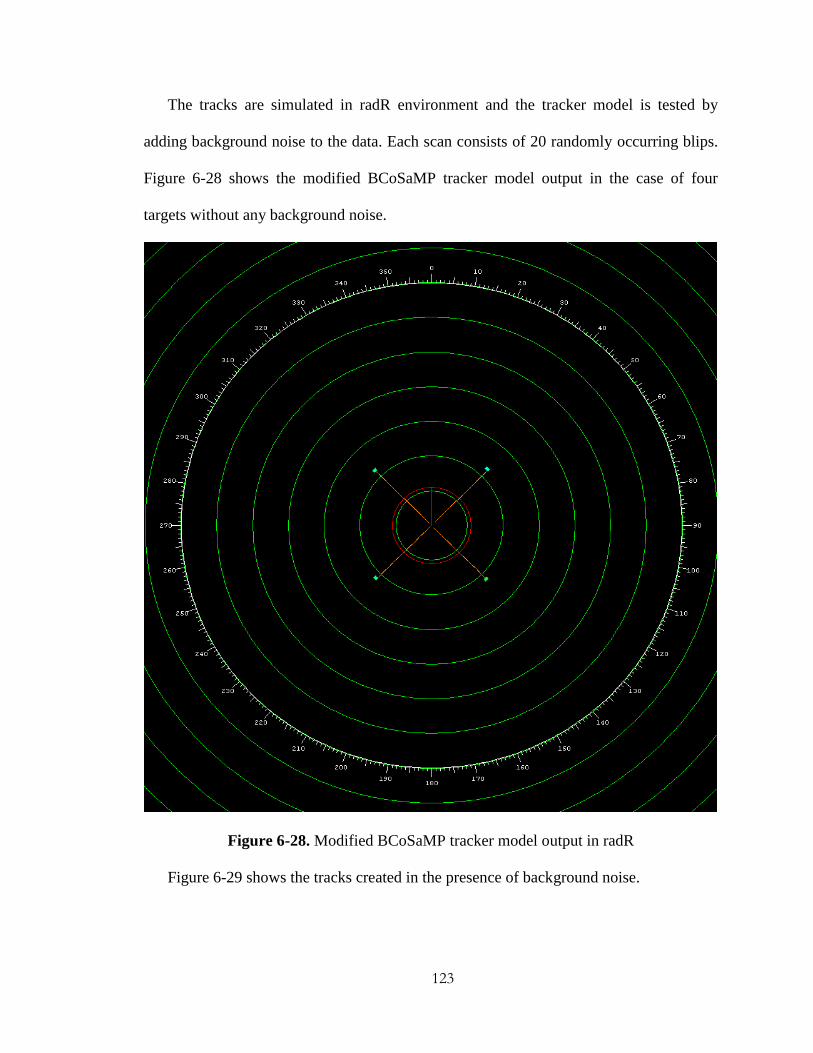
123
The tracks are simulated in radR environment and the tracker model is tested by
adding background noise to the data. Each scan consists of 20 randomly occurring blips.
Figure 6-28 shows the modified BCoSaMP tracker model output in the case of four
targets without any background noise.
Figure 6-28. Modified BCoSaMP tracker model output in radR
Figure 6-29 shows the tracks created in the presence of background noise.

124
Figure 6-29. Modified BCoSaMP tracker model output with noise in radR
The performance of four tracker models developed is analyzed with the error rates of
estimated tracks. Figure 6-30 shows the error rates in the case of single track. It can be
seen that the modified BCoSaMP has the least error compared to the other models.

125
Figure 6-30. Error rates of four tracker models for a single track
Figures 6-31 to 6-34 shows the error rates of each track in the simulated multi target
environment for the four tracker models. It can be seen that the particle filter has the
lowest error rate compared to other models with the increase in number of scans.
0 5 10 15 20 250
0.5
1
1.5
2
2.5
3
3.5
4
4.5
Number of scans
Err
or
(perc
enta
ge)
Error Rates of Tracking Algorithms
Kalman filter
Particle filter
BCoSaMP
Modified BCoSaMP

126
Figure 6-31. Error rates of track 1 for four tracker models in multi target environment
Figure 6-32. Error rates of track 2 for four tracker models in multi target environment
0 5 10 15 20 250
1
2
3
4
5
6
7
8
9
Number of scans
Err
or
(perc
enta
ge)
Error rate of track 1
Kalman filter
Particle Filter
BCoSaMP
Modified BCoSaMP
0 5 10 15 20 250
2
4
6
8
10
12
14
Number of scans
Err
or
(perc
enta
ge)
Error rate of track 2
Kalman filter
Particle Filter
BCoSaMP
Modified BCoSaMP

127
Figure 6-33. Error rates of track 3 for four tracker models in multi target environment
Figure 6-34. Error rates of track 4 for four tracker models in multi target environment
0 5 10 15 20 250
2
4
6
8
10
12
14
Number of scans
Err
or
(perc
enta
ge)
Error rate of track 3
Kalman filter
Particle Filter
BCoSaMP
Modified BCoSaMP
0 5 10 15 20 250
1
2
3
4
5
6
7
8
9
Number of scans
Err
or
(perc
enta
ge)
Error rate of track 4
Kalman filter
Particle Filter
BCoSaMP
Modified BCoSaMP

128
6.4 Simulation of Four Tracker Models with Marine Radar Data:
A balloon with a GPS is used to calibrate the radar as its path was tracked. The path
of the balloon was observed to be random on the radar screen with very low velocity. The
track of the balloon seen in the radar display is shown in Figure 6-35.
Figure 6-35. Track of the balloon moving away from the radar
The tracker models are used to identify if the balloon is being tracked and outputs are
shown in Figures 6-36 to 6-40. Due to low velocity and random motion of the balloon the
tracks formed are not continuous and a lot of noise also gets included when the tracks are
formed. The particle filter is the only model that estimates the target path closely with
noise included along with its path. The other models just track the balloon at certain
points along the track. The optimized values are given in Table 6.1.
100 200 300 400 500 600 700 80065
70
75
80
85
90
95
100
Range (meters)
Heig
ht
(mete
rs)
Track of target moving away from radar

129
Table 6.1: Optimized blip processing parameters
Parameters Optimized Values
Noise cutoff 0
Learning scans 15
Old stats weighting 0.95
Hot score 2.8
Cold score 2.8
Samples per cell 4
Pulses per cell 4
Min. blip samples 30
Max. blip samples 50000
Max. blip area 50000
Min. blip area 300
Min. angular span 2
Max. angular span -1
Min. radial span 2
Max. radial span -1
Tracker models with recommended blip processing parameters given in Chapter 3
and with a set of optimized values for blip processing are analyzed. Variation in blip
processing parameters does not affect tracking significantly. BCoSaMP model does not
track the target when the balloon is moving away from the radar for optimized blip
processing parameters.

130
Figure 6-36. Kalman filter tracking of the balloon
Figure 6-37. Particle filter tracking of the balloon
100 200 300 400 500 600 700 80040
60
80
100
120
140
160
180
Range (meters)
Heig
ht
(mete
rs)
Kalman filter tracking
Actual target track
Kalman filter track
Kalman tracking with optimized values
100 200 300 400 500 600 700 800 90040
60
80
100
120
140
160
180
200
Range (meters)
Heig
ht
(mete
rs)
Particle filter tracking
Actual target track
Particle filter tracking
Particle filter tracking with optimized values

131
Figure 6-38. BCoSaMP tracking of the balloon
Figure 6-39. Modified BCoSaMP tracking of the balloon
100 200 300 400 500 600 700 800
60
70
80
90
100
110
120
Range (meters)
Heig
ht
(mete
rs)
BCoSaMP Tracking
Actual target track
BCoSaMP tracking
100 200 300 400 500 600 700 80050
60
70
80
90
100
110
120
130
Range (meters)
Heig
ht
(mete
rs)
Modified BCoSaMP Tracking
Actual target track
Modified BCoSaMP tracking
Modified BCoSaMP tracking with optimized values

132
Figure 6-40. Multi-frame correspondence tracking of the balloon
Nearest neighbor model is not discussed because the tracks were very sensitive to
noise that the track of the balloon was overlapped with many false alarms making the
track of the balloon undetectable.
Figure 6-41 shows the track of the balloon moving towards the radar. Figures 6-42 to
6-46 show the tracks detected by the tracker models.
100 200 300 400 500 600 700 80040
60
80
100
120
140
160
180
Range (meters)
Heig
ht
(mete
rs)
Multi-frame Tracking
Actual target track
MF tracking
MF tracking with optimized values

133
Figure 6-41. Track of the balloon moving towards the radar
Figure 6-42. Kalman filter tracking of the balloon
100 200 300 400 500 600 70050
55
60
65
70
75
80
85
90
95Track of target moving towards radar
Range (meters)
Heig
ht
(mete
rs)
100 200 300 400 500 600 70050
100
150
200
Range (meters)
Heig
ht
(mete
rs)
Kalman filter tracking
Actual target track
Kalman filter track
Kalman tracking with optimized values

134
Figure 6-43. Particle filter tracking of the balloon
Figure 6-44. BCoSaMP tracking of the balloon
100 200 300 400 500 600 700 80040
50
60
70
80
90
100
110
Range (meters)
Heig
ht
(mete
rs)
Particle filter tracking
Actual target track
Particle filter tracking
Particle filter tracking with optimized values
100 200 300 400 500 600 70050
60
70
80
90
100
110
Range (meters)
Heig
ht
(mete
rs)
BCoSaMP Tracking
Actual target track
BCoSaMP tracking
BCoSaMP tracking with optimized values

135
Figure 6-45. Modified BCoSaMP tracking of the balloon
Figure 6-46. Multi-frame Correspondence tracking of the balloon
100 200 300 400 500 600 70050
60
70
80
90
100
110
Range (meters)
Heig
ht
(mete
rs)
Modified BCoSaMP tracking
Actual target track
Modified BCoSaMP tracking
Modified BCoSaMP tracking with optimized values
100 200 300 400 500 600 700 80050
60
70
80
90
100
110
Range (meters)
Heig
ht
(mete
rs)
Multi-frame tracking of target
Actual target track
MF tracking
MF tracking with optimized values

136
Tracker models are evaluated using marine radar data collected with T-bar antenna in
the vertical mode. The number of targets identified and the false alarm rates of the tracker
models are compared. Figure 6-47 shows the number of targets detected.
Figure 6-47. Number of targets detected
The computation time of various algorithms are given in Table 6.2:
Table 6.2: Computation time of the tracker models
Tracker Model Computation Time (minutes)
Multi-Frame 24
Kalman filter 75
Particle Filter 208
BCoSaMP 120
Modified BCoSaMP 180
The computation time is calculated for marine radar data that was collected for 2
hours 32 minutes.
0
500
1000
1500
2000
2500
Nu
mb
er o
f T
arg
ets
Target Detection with Marine Radar Data
True Tracks
False Alarms
Total

137
6.5 Summary:
The performance of various tracker models is discussed by simulating tracker models
with various data. Nearest neighbor tracker model is not discussed as it contains a lot of
noise and true tracks are lost when there is high amount of noise. The particle filter has
high computation time due to the use of large number of particles however in marine
radar data it was the only method to track the target accurately. Particle filter has the
highest detection rates but is affected by noise. The BCoSaMP also gives reliable output
as the false alarms are less and has detection rates close to particle filter. BCoSaMP can
be used when less computation time is required. These models help in increasing the data
processing reliability and accuracy compared to the current tracking models in radR.

139
Chapter 7
Conclusion and Future Work
7.1 Conclusion:
Radar tracking is used in the study of bird flight patterns. The work will help in
understanding the behavior of bird towards man-made structures. Tracking birds is
challenging in radar data due to noise, clutter and wide coverage area of the radar. Four
tracker models were developed considering a linear system, nonlinear system and sparse
data conditions to identify the most apt tracker model for radar data. The tracker models
performance is analyzed based on three types of data sets which are:
One simulated track: BCoSaMP and modified BCoSaMP have the least error
rate. The newly developed model has 1% error and gives the most ideal output.
Four simulated tracks with noise: In simulated data with four tracks show
various error rates for all models. The least error rate varies for each track. It is
also shown that addition of noise results in induced error in the created tracks.
Calibration of Marine radar data via balloon movement: The balloon was
detected well by the particle filter compared to other models. The number of
targets identified is high for particle filter but it is very sensitive to noise. The
BCoSaMP model also has reliable output as the identification rates are closer to
particle filter and has significantly less false alarms.

140
The analysis with various data shows that particle filter has the most optimum tracking
and high identification rates compared to the multi-frame model in radR. BCoSaMP also
gives reliable results based on the fact that there is significant decrease in false alarm
rates. The tracker models should be selected based on the data type and presence of noise.
These plugins are developed to aid in data processing ensuring higher reliability and
accuracy.
7.2 Future Work:
Tracker models can be further improved to reduce the false alarm rates. False alarms
can be reduced by defining a dynamic system to identify the noise levels. However
implementation for radar data can be challenging owing to the fact that noise levels are
time variant. In these models, only nearest neighbor data association is used this can also
be improved by using better data association techniques and additional gating techniques
for thresholding. The computation time can be reduced by parallelizing the tracker
algorithms.

141
References
[1] Migratory Bird Mortality Available from: http://www.fws.gov/birds/mortality-
fact-sheet.pdf
[2] American Bird Conservancy Available from:
http://www.abcbirds.org/abcprograms/policy/collisions/wind_farms.html
[3] Bird Fatalities at Wind Energy Sites:
http://www.fws.gov/midwest/GreatLakes/windpowerpresentations/Thelander.pdf
[4] David P. Young, Jr., Dale Strickland, Wallace P. Erickson, Kimberly J. Bay and
Ron Canterbury, Baseline Avian Studies Mount Storm Wind Power Project, Grant
County, West Virginia, April 23, 2004 from: http://www.west-
inc.com/reports/mount_storm_final.pdf
[5] Mark E. Hostetler and Martin B. Main, Florida Monitoring Program: Point Count
Method to Survey Birds from: http://edis.ifas.ufl.edu/pdffiles/UW/UW14000.pdf
[6] Verhoef, J.P., Westra, C.A., Korterink, H., and Curves, A., WT-Bird A Novel
Bird Impact Detection System from:
http://www.ecn.nl/docs/library/report/2002/rx02055.pdf
[7] Willem W. Verstraeten, Bart Vermeulen, Jan Stuckens, Stefaan Lhermitte,
Dimitry Van der Zande, Marc Van Ranst and Pol Coppin, Webcams for Bird Detection
and Monitioring: A Demonstartion Study, Sensors, 2010, Vol.10(4): p. 3480-3503.

140
[8] Radio Telemetry and bird movements from:
ftp://ftp.fao.org/docrep/fao/010/a1521e/a1521e07.pdf
[9] Brian A. Cooper, Use of Radar for Wind-Power Related Avian Research, National
Avian-Wind Power Planning Meeting Proceedings, 1995, from:
http://old.nationalwind.org/publications/wildlife/avian95/avian95-08.htm
[10] James P. Ferry and J. Oren Bumgarner, Community Detection and Tracking on
Networks from a Data Fusion Perspective, Jan 6, 2012, from:
http://arxiv.org/pdf/1201.1512.pdf
[11] Frederick C. Lincoln, Steven R. Peterson and John L. Zimmerman, U.S. Fish and
Wildlife Service, Migration of Birds, 1998, from:
http://library.fws.gov/Circulars/Mig_of_Birds_16_98.pdf
[12] Felix iechti and Bruno Bruderer, Quantification of Nocturnal Bird Migration by
Moonwatching: Comaprison with Radar and Infrared Observations, Journal of Field
Ornitology, 1995, Vol. 66(4): p. 457-652.
[13] Sirko Molau, Michael Pitz, Ralf Schluter and Hermann Ney, Computing Mel-
Frequency Cepstral Coefficients on the Power Spectrum, IEEE International Conference
on Acoustics, Speech and Signal Processing, 2001, Vol. 1:p. 73-76.
[14] Amara Graps, An Introduction to Wavelets, IEEE Computational Science and
Engineering, 1995, CA, Vol. 2(2):p. 50-61.
[15] S. Bastas, M. W. Majid, G. Mirzaei, J. Ross, M. Jamali, P. V. Gosevski, J.
Frizado, P. V. Bingman, A Novel Feature Extraction Algorithm for Classification of Bird
Flight Calls, IEEE International Symposium on Circuits and Systems on Circuits (ISCAS
2012), 2012.

141
[16] Sonobat from: http://sonobat.com
[17] G. Mirzaei, W. M. Majid, J. Ross, J. Frizado, P. V. Gosevski, and V. Bingman,
The application of Evolutionary Neural Network for Bat Echolocation Calls Recognition,
IEEE International Joint Conference on Neural Networks, 2011, p. 1106-1111.
[18] M. Piccardi, Background Subtraction Techniques: a review, IEEE International
Conference on systems, Man and Cybernetics, 2004, p. 3099-3104.
[19] R. C. Gonzalez, R. E. Woods, Digital Image Processing, Pearson, 2009.
[20] Golrokh Mirzaei, Mohammad Wadood Majid, Jeremy Ross, Mohsin M. Jamali,
Joseph Frizado, Peter V. Gorsevski, Verner P. Bingman, Avian Detection and Tracking
Algorithm using Infrared Imaging, IEEE International Conference on Electro/Information
Technology, 2012.
[21] WSR88D from: http://www.roc.noaa.gov/WSR88D
[22] Sidney A. Gauthreaux and Carroll G. Belser, Bird Movements on Doppler
Weather Surveillance Radar, Birding, December 2003, Vol. 35(6): pp. 616-628.
[23] Theodore R. Simons, Frank R. Moore and Sidney A. Gauthreaux, Mist Netting
Trans-Gulf Migrants at Coastal Stopover Sites: The Influence of Spatial and Temporal
Variability on Capture Data, Studies in Avian Biology, 2004, Vol.29: p.135-143.
[24] Adriaan M. Dokter, Felix Liechti, Herbert Stark, Laurent Delobbe, Pierre Tabary
and Iwan Holleman, Bird Migration Flight Altitudes Studied by a Network of
Operational Weather Radars, Journal of The Royal Society Interface, June 2 , 2010, p. 1-
14.
142
[25] Brian A. Cooper, Robert H. Day, Robert J. Ritchie and Clayton L. Cranor, An
Improved Marine Radar System for Studies of Bird Migration, Journal of Field
Ornithology, 1991, Vol. 62(3): p. 367-377.
[26] Ning Huansheng, Chen Weishi, Mao Xia and Li Jing, Bird-Aircraft Strike
Avoidance Radar, IEEE A&E Systems Magazine, January 2010, Vol. 25(1): p. 19-28.
[27] Philip D. Taylor, John M. Brzustowski, Carolyn Matkovich, Michael L.
Peckford and Dave Wilson, radR: An Open-source Platform for Acquiring and Analysing
Data on Biological Targets Observed by Surveillance Radar, BMC Ecology, 2010, from:
http://www.radr-project.org/
[28] Sidney A. Gauthreaux, Jr and Carroll G.Belser, Radar Ornithology and
Biological Conservation, The Auk, 2003, Vol. 120(2): p. 266-277.
[29] Edward J. Zakrajsek and John A. Bissonette, Nocturnal Bird-Avoidance
Modeling with Mobile-Marine Radar, 2001 Bird Strike Committee, Calgary, AB, 2001,
Available from:
http://digitalcommons.unl.edu/cgi/viewcontent.cgi?article=1029&context=birdstrike2001
[30] Brian A. Cooper, Robert H. Day, Robert J.Ritchie and Clayton L. Cranor, An
Improved Marine Radar System for Studies of Bird Migration, 1991, Journal of Filed
Ornithology, Vol. 62(3): p. 367-377.
[31] Kathleen E. Moore and Judith A Henningson, Intergration of NEXRAD, Marine
Radar, SODAR and Conventional Anemometry for Avian Risk Assessment, from:
https://ams.confex.com/ams/90annual/techprogram/paper_164352.htm
[32] Peter Weber, Tim J. Nohara and Sidney Gauthreaux, Affordable, Real-Time, 3-D
Avian Radar Networks for Centralized North American Bird Advisory Systems, Bird
143
Strike 2005, Vancouver, Canada, August 2005, from:
http://digitalcommons.unl.edu/cgi/viewcontent.cgi?article=1006&context=birdstrike2005
[33] Lindsay I Smith, A Tutorial on Principal Components Analysis, February 2002,
from: http://www.sccg.sk/~haladova/principal_components.pdf
[34] Ziv Yaniv, Median Filtering, from:
http://isiswiki.georgetown.edu/zivy/writtenMaterial/median.pdf
[35] Chin-Ya Huang and Mon-Ju Wu, Image Segmentation, 2006, from:
http://homepages.cae.wisc.edu/~ece533/project/f06/huang_wu_rpt.pdf
[36] Wayne, Lin Wei-Cheng and Wu Ja-Ling, Mathematical Morphology and its
Applications on Image Segmentation, June 2007, from: http://www.fmi.uni-
sofia.bg/courses/biomed/morphgeom/thesis_morphology.pdf
[37] Bird Monitoring using the Mobile Avian Radar System (MARS) by Geo-
Marine, Inc, 2004 from: http://www.boemre.gov/offshore/PDFs/CWFiles/67.pdf
[38] Heiko Schmaljohann, Felix Liechti, Erich Bachler, Thomas Steuri and Bruno
Bruderer, Quantification of Bird Migration by Radar – a Detection Probability Problem,
Journal Compilation at British Ornithologists Union, 2008, Vol. 150: p. 342-355.
[39] Richard Walls, Monitoring Avian Movement using Bird Detection Radar;
Impacts of Nocturnal Movement on Flight Safety at a Military Aerodrome, International
Bird Strike Committee, May 2005 from: http://www.int-
birdstrike.org/Athens_Papers/IBSC27%20WPVIII-4.pdf
[40] Michael L. Peckford and Philip D. Taylor, Within Night Correlations between
Radar and Ground Counts of Migrating Songbirds, Journal of Field Ornithology, 2008,
Vol. 79(2): p. 207-214

144
[41] Study Components Available from: http://www.acciona-
na.com/getattachment/837f72a6-dc5c-4eaa-995a-20794aa247bd/
[42] D. F. Bertram, L. Cowen and A. E. Burger, Use of Radar for Monitoring
Colonial Burrow-Nesting Seabirds, Journal of Field Ornithology, 1999, Vol. 70, No.2: p.
145-282.
[43] Alan E. Burger, Behavior and Numbers of Marbled Murrelets Measured with
Radar, Journal of Field Ornithology, Vol. 68(2): p. 208-223.
[44] DeTect Inc Available from: http://www.detect-inc.com/
[45] T. Adam Kelly, McLaughlin and Smith, New Ornithological Radar Technologies
for Bird and Bat Discrimination and Species Identification, 2007, Available from:
http://www.detect-
inc.com/downloads/Ornithological%20Radar%20Technologies%20for%20Bird%20&%2
0Bat%20Discrimination%20&%20Species%20Identification%20TAK%20et%20al%206
7.pdf
[46] Todd J. Mabee, Brian A. Cooper, Jonathan H. Plissner and David P. Young,
Nocturnal Bird Migration Over an Appalachian Rigde at a Proposed Wind Power Project,
Available from: http://onlinelibrary.wiley.com/doi/10.2193/0091-
7648%282006%2934%5B682:NBMOAA%5D2.0.CO;2/abstract
[47] Robert W. McFarlane and James Lester, Determination of Nearshore Seabird
Density on the Upper Texas Coast, 2005, from:
http://www.seco.cpa.state.tx.us/zzz_re/re_wind_projects-bird.pdf

145
[48] Paul Kerlinger and Sidney A. Gauthreaux, Jr., Seasonal Timing, Geographic
Distribution and Flight Behaviour of Broad-Winged Hawks During Spring Migration in
South Texas: A radar and Visual Study, October 1985, The Auk, Vol. 102: p. 735-743.
[49] Sidney Gauthreaux, Jr and CUROL Laboratory from :
http://old.nationalwind.org/events/wildlife/2006-3/presentations/birds/gauthreaux.pdf
[50] FURUNO Installation Manual Available from: FURUNO Electrical Co. LTD
[51] FURUNO Operator’s Manual Available from: FURUNO Electrical Co. LTD
[52] RTI IntegRadar XIR3000 Manual Available from: Russell Technologies Inc.
[53] RadarSample Usage Notes Available from: Russell Technologies Inc.
[54] radR Available from: http://www.radr-project.org/
[55] Methods of Estimation from:
http://web.as.uky.edu/statistics/users/viele/sta321s98/estimation/estimation.html
[56] Track Radar Systems Available from: http://ed-thelen.org/MMS-150-Ch04.pdf
[57] Apostolos N. Papadopoulos, Nearest Neighbor Search, Springer Publishers,
December 6, 2010.
[58] Knuth DE: The Stanford GraphBase: A platform for combinatorial Computing.
New York: ACM Press, 1993, from: http://www-cs-faculty.stanford.edu/~uno/sgb.html
[59] Knuth DE: The Stanford GraphBase package. Available from: http://www-cs-
faculty.stanford.edu/~knuth/sgb.html
[60] Shafique K, Shah M, A Noniterative Greedy Algorithm for Multiframe Point
Correspondence, IEEE Transactions on Pattern Analysis and Machine Intelligence, 2005,
Vol. 27(1): p. 51-65.

146
[61] D. M. Akbar Hussain, David Hicks, Daniel Ortiz-Arroyo, Shaiq A. Haq and Zaki
Ahmed, A Case Study: Kalman & Alpha-Beta Computation under High Correlation,
Proceedings of the International MultiConference of Engineers and Computer Scientists
2008, Hong Kong, 2008, Vol. 1: p. 19-21.
[62]Aaron D.Lanterman, Passive Radar Imaging and Target Recognition using
Illuminators of Opportunity, RTO SET Symposium, Norway, October 2004, Vol. 24: p.
1-9.
[63] Sun-Mog Hong and Young-Hun Jung, Optimal Scheduling of Track Updates in
Phased Array Radars, IEEE transactions on Aerospace and Electronic Systems, 1998,
Vol. 34(3): p. 1016-1022.
[64] David Bizup, A Centripetal Acceleration Statistic for Tracking Maneuvering
Targets with Radar, from:
http://www.dodccrp.org/events/7th_ICCRTS/Tracks/pdf/095.PDF
[65] John N. Briggs, Target Detection by Marine Radar, IEE Radar, Sonar,
Navigation and Avionics Series 16, 2004.
[66] Mathew Connor, Kathleen Haas and Alexander Volfson, Multiple Target
Tracking, 2008, from: http://www.wpi.edu/Pubs/E-project/Available/E-project-101608-
152650/unrestricted/Group31Final.pdf
[67] X. Rong Li and VesselinP.Jilkov, A Survey of Maneuvering Target Tracking –
Part III: Measurement Models, SPIE Conference on Signal and Data Processing of Small
Targets, CA, August 2001, from: http://coe.uno.edu/ee/ISL/Reprints/M3-distribute.pdf

147
[68] Bing-Fei Wu and Jhy-Hong Juang, Two Target Tracking Design Patterns for a
Real Time Phased Array Radar System, International Journal of Engineering and
Industries, September 2011, Vol. 2(3): p. 141-149.
[69] Hazem Kamel and K.H. Moustafa, High Performance Target Tracking Using
Tracker Fusion in a Track-While-Scan Radar, Conference on Aerospace Sciences and
Aviation Technology ASAT-13-CM-15, Egypt, May 2009, from:
http://www.mtc.edu.eg/ASAT13/pdf/CM15.pdf
[70] G.L. Soares, A. Arnold-Bos, L. Jaulin, J.A. Vasconcelos and C.A. Maia, An
Interval-based Target Tracking Approach for Range-only Multistatic Radar, IEEE
transactions on Magnetics, 2008, Vol. 44(6):p. 1350 - 1353.
[71] Bhavana Manjunath, Jun J. Zhang, Antonia Papandreou-Suppappola and Darryl
Morrell, Sensor Scheduling with Waveform Design for Dynamic Target Tracking using
MIMO Radar, Forty-Third Asilomar Conference on Signals, Systems and Computers,
Asilomar, 2009, p. 141-145.
[72] Vijay Venkataraman, Xin Fan and Guoliang Fan, Integrated Target Tracking and
Recognition via Joint Appearance-Motion Generative Models, IEEE Computer Society
Conference on Computer Vision and Pattern Recognition Workshops, June 2008, p. 1-8.
[73] Yunqian Ma, Qian Yu and Isaac Cohen, Multiple Hypothesis Target Tracking
Using Merge and Split of Graph's Nodes, ISVC’06 Proceedings of the Second
International Conferences on Advances in Visual Computing, 2006, Vol. 1:p. 783-792.
[74] A. Benavoli, L.Chisci, A.Farina, S. Immediata, L. Timmoneri and G. Zappa,
Knowledge-Based System for Multi-Target Tracking in a Littoral Environment, IEEE
transactions on Aerospace and Electronic Systems, July 2006, Vol. 42(3):p. 1100-1119.

148
[75] Curtis B. Storlie, Thomas C. M. Lee, Jan Hannig and Douglas Nychka, Tracking
of Multiple Merging and Splitting Targets: A Statistical Perspective, Statistica Sinica 19,
2009, p. 1-52.
[76] Inseok Hwang, Hamsa Balakrishnan, Kaushik Roy and Claire Tomlin, Multiple-
Target Tracking and Identity Management in Clutter, with Application to Aircraft
Tracking, American Control Conference, Vol. 4: p. 3422-3428.
[77] Dae-Sung Jang and Han-Lim Choi, Pulse Interleaving for Multi-target Tracking
on Pulse Doppler Phased Array Radar, 2011, from:
http://lics.kaist.ac.kr/files/JangChoi_RadarCon12.pdf
[78] Daniel Svensson, Target Tracking in Complex Scenarios, Sweden, 2010, from:
http://publications.lib.chalmers.se/records/fulltext/125955.pdf
[79] Markus Buhren and Bin Yang, Initialization Procedure for Radar Target
Tracking without Object Movement Constraints, ITST ’07.7th
International Conference
on ITS, 2007, p.1-6.
[80] Kiril Alexiev, A MATLAB Tool for Development and Testing of Track
Initiation and Multiple Target Tracking Algorithms, Information & Security, 2002, Vol.
9:p.166-174.
[81] Y. Boers and J.N. Driessen, Multitarget Particle Filter Track Before Detect
Application, IEEE Proceedings Radar, Sonar and Navigation, 2003, Vol. 151: p. 351-357.
[82] Pavlina Konstantinova, Milen Nikolov and Tzvetan Semerdjiev, A Study of
Clustering Applied to Multiple Target Tracking Algorithm, International Conference on
Computer Systems and Technologies- CompSysTech ‘2004, 2004, p. 1-6.

149
[83] Jehangir Khan, Smail Niar, Atika Menhaj, Yassin Elhillali and Jean Luc
Dekeyser, An MPSoC Architecture for the Multiple Target Tracking Application in
Driver Assistant System, ASAP ’08 Proceedings of the 2008 International Conference on
Application – Specific Systems, Architectures and Processors, 2008, p. 126-131.
[84] Godrich, H., Chiriac, V.M. Haimovich, A.M. Blum and R.S., Target Tracking in
MIMO Radar Systems: Techniques and Performance Analysis, IEEE Radar Conference,
2010, p.1111-1116.
[85] V.P.S. Naidu, Fusion of IRST and Radar Measurements for 3D Target Tracking,
IE(I) Journal-AS, July 2009, p. 10-16.
[86] Zhiqiang Hou and Chongzhao Han, A Target Tracking System based on Radar
and Image Fusion, 2003. Proceedings of the Sixth International Conference of
Information Fusion, 2003, Vol.2: p. 1426-1432.
[87] Volkan Cevher, Milind Borkar and James H. McClellan, A Joint Radar-Acoustic
Particle Filter with Acoustic Propagation Delay Compensation, 2008, from:
http://infoscience.epfl.ch/record/151450
[88] Edwin Chong and Louis L. Scharf, Intergrated Radar Imaging, Target Tracking,
and Sensor Scheduling, May 2006, from:
http://www.dtic.mil/dtic/tr/fulltext/u2/a448056.pdf
[89] Roberto Togneri, Estimation Theory for Engineers, August 2005,
http://www.ee.uwa.edu.au/~roberto/teach/Estimation_Theory.pdf
[90] Peter S. Maybeck, Stochastic Models, Estimation and Control, 1999, from:
http://www.cs.unc.edu/~welch/kalman/media/pdf/maybeck_ch1.pdf

150
[91] DusanKocur, Jan Gamec, Maria Svecova, Maria Gamcova and Jana Rovnakova,
Imaging Method: An Efficient Algorithm for Moving Target Tracking by UWB Radar,
Acta Polytechnica Hungarica, 2010, Vol. 7(3):p. 5-24.
[92] Wing Ip Tam, and D. Hatzinakos, An Adaptive Gaussian Sum Algorithm for
radar Tracking, IEEE Internation Conference on Communications, 1997, Vol. 3: p. 1351-
1355.
[93] Jong Hyun Lim, I-Jeng Wang, Andreas Terzis, Tracking a Non-cooperative
Mobile Target Using Low-Power Pulsed Doppler Radars, from:
http://hinrg.cs.jhu.edu/joomla/images/stories/radar.pdf
[94] Tony Lacey, Tutorial: The Kalman Filter from:
http://mpdc.mae.cornell.edu/Courses/UQ/kf1.pdf
[95] Greg Welch and Gary Bishop, An Introduction to the Kalman Filter, TR 95-041,
July 24, 2006, from: http://www.cs.unc.edu/~welch/media/pdf/kalman_intro.pdf
[96] Dan Simon, Kalman Filtering, Embedded Systems Programming, 2007,
Available from: jettronics.de/trac/projects/export/169/.../kalman-dan-simon.pdf
[97] Maria Isabel Ribeiro, Kalman and Extended Kalman Filters: Concept,
Derivations and Properties, 2004 from: http://users.isr.ist.utl.pt/~mir/pub/kalman.pdf
[98] Gabriel A. Terejanu, Extended Kalman Filter Tutorial, from:
http://users.ices.utexas.edu/~terejanu/files/tutorialEKF.pdf
[99] Maria Isabel Ribeiro, Kalman and Extended Kalman Filters: Concept, Derivation
and Properties, February 2004, from: http://users.isr.ist.utl.pt/~mir/pub/kalman.pdf

151
[100] Eric A. Wan and Rudolph van der Merwe, The Unscented Kalman Filter for
Nonlinear Estimation, IEEE 2000 Adaptive Systems for Signal Processing,
Communications and Control Symposium, 2000, p. 153-158.
[101] Gabriel A. Terejanu, Unscented Kalman Filter Tutorial, NY, from:
http://users.ices.utexas.edu/~terejanu/files/tutorialUKF.pdf
[102] Eleni N. Chatzi and Andrew W. Smyth, The Unscented Kalman Filter and
Particle Filter Methods for Nonlinear Structural System Identification with Non-
Collocated Heterogeneous Sensing, Journal of Structural Control and Health Monitoring,
NY, 2008, from: http://www.civil.columbia.edu/smyth/papers/stcdoc_rev_4.pdf
[103] Edita Kolarova, An Application of the Kalman-Bucy Filter to Electrical
Circuits, August 2007, from:
http://math.fce.vutbr.cz/~pribyl/workshop_2007/prispevky/KolarovaA.pdf
[104] S. Gillijins, O. Barrero Mendoza, J. Chandrasekar, B. L. R. De Moor, D. S.
Bernstein and A. Ridley, What is the Ensemble Kalman Filter and How Well Does it
Work?, American Control Conference, June 2006, from:
http://www.math.pitt.edu/~cbsg/Materials/Gillijns-etal.pdf
[105] E. Kalnay, Hong Li and T. Miyoshi, Introduction to Ensemble Kalman Filter,
JCSDA Summer Colloquium, 2009, from:
http://www.jcsda.noaa.gov/documents/meetings/2009summercoll/Kalnay1_KalmanFilter.
[106] Atef Isaac, Peter Willett and Yaakov Bar-Shalom, Quickest Detection and
Tracking of Spawning Targets Using Monopulse Radar Channel Signals, IEEE
Transactions on Signal Processing, August 2006, Vol. 56: p. 1302-1308.

152
[107] Richard Karlsson and Fredrik Gustafsson, Monte Carlo Data Association for
Multiple Target Tracking, from: http://www.control.isy.liu.se/~fredrik/reports/01iee.pdf
[108] Matthias Muhlich, Particle Filters an Overview from: http://user.uni-
frankfurt.de/~muehlich/sci/TalkBucurestiMar2003.pdf
[109] M. SanjeevArulampalam, Simon Maskell, Neil Gordon and Tim Clapp, A
Tutorial on Particle Filters for Online Nonlinear/Non-Gaussian Bayesian Tracking, IEEE
Transactions on Signal Processing, February 2002, Vol. 50(2): p. 174 - 188.
[110] Niclas Bergman, Recursive Bayesian Estimation: Navigation and Tracking
Applications, 1999, from:
http://www.control.isy.liu.se/research/reports/Ph.D.Thesis/PhD579.pdf
[111] D. Needell and J.A. Tropp, CoSaMP: Iterative Signal Recovery from
Incomplete and Inaccurate Samples, Information theory and Applications, July 2008,
from: http://users.cms.caltech.edu/~jtropp/papers/NT08-CoSaMP-Iterative-preprint.pdf
[112] Petros Boufounos, Marco F. Duarte and Richard G. Baraniuk, Sparse Signal
Reconstruction from Noisy Compressive Measurements using Cross Validation, from:
http://dsp.rice.edu/sites/dsp.rice.edu/files/publications/conference-paper/2007/sparse-ssp-
2007.pdf
[113] Irina F. Gorodnitsky, Bhaskar D. Rao, Sparse Signal Reconstruction from
Limited Data Using FOCUSS: A Re-weighted Minimum Norm Algorithm, IEEE
proceedings on signal processing, March 1997, Vol. 45(3):p. 600-616.
[114] Emmanuel J. Candes, The Restricted Isometry Property and Its Implications for
Compressed Sensing, Comptes Rendus Mathematique, 2008, Vol. 346:p. 589-592.

153
[115] Joel A. Tropp, Just Relax: Convex Programming Methods for Identifying
Sparse Signals in Noise, IEEE Transactions on Information Theory, 2006, Vol. 52:pp.
1030- 1051.
[116] Dr. Volkan Cevher and Andrew Waters, The CoSamp Algorithm, October 12,
2008, from: http://www.ece.rice.edu/~vc3/elec633/CoSaMP.pdf
[117] Satyabrata Sen and Arye Nehorai, Sparsity-Based Multi-Target Tracking Using
OFDM Radar, IEEE Transactions on Signal Processing, April 2011, Vol. 59(4):p. 1902-
1906.
[118] Ottawa Wildlife Refuge from:
http://www.fws.gov/refuges/profiles/index.cfm?id=31540