enhancing neural-network performance via assortativity

8/7/2019 Enhancing neural-network performance via assortativity

http://slidepdf.com/reader/full/enhancing-neural-network-performance-via-assortativity 1/9

a r X i v : 1 0 1 2 . 1 8 1

3 v 1

[ c o n d - m a t . d i s

- n n ] 8 D e c 2 0 1 0

Enhancing neural-network performance via assortativity

Sebastiano de Franciscis, Samuel Johnson, and Joaquın J. TorresDepartamento de Electromagnetismo y Fısica de la Materia, and

Institute Carlos I for Theoretical and Computational Physics,

Facultad de Ciencias, University of Granada, 18071 Granada, Spain.

The performance of attractor neural networks has been shown to depend crucially on the het-erogeneity of the underlying topology. We take this analysis a step further by examining the effectof degree-degree correlations – or assortativity – on neural-network behavior. We make use of amethod recently put forward for studying correlated networks and dynamics thereon, both ana-lytically and computationally, which is independent of how the topology may have evolved. Weshow how the robustness to noise is greatly enhanced in assortative (positively correlated) neuralnetworks, especially if it is the hub neurons that store the information.

PACS numbers: 64.60.aq, 84.35.+i, 89. 75.Fb, 87.85.dm

I. BACKGROUND

For a dozen years or so now, the study of complexsystems has been heavily influenced by results from net-

work science – which one might regard as the fusion of graph theory with statistical physics [1, 2]. Phenomenaas diverse as epidemics [3], cellular function [4], power-grid failures [5] or internet routing [6], among many oth-ers [7], depend crucially on the structure of the under-lying network of interactions. One of the earliest sys-tems to have been described as a network was the brain,which is made up of a great many neurons connected toeach other by synapses [8–11]. Mathematically, the firstneural networks combined the Ising model [12] with theHebb learning rule [13] to reproduce, very successfully,the storage and retrieval of information [14–16]. Neu-rons were simplified to binary variables (like Ising spins)representing firing or non-firing cells. By considering thetrivial fully-connected topology, exact solutions could bereached, which at the time seemed more important thanattempting to introduce biological realism. Subsequentwork has tended to focus on considering richer dynamicsfor the individual cells rather than on the way in whichthese are interconnected [11, 17, 18]. However, the topol-ogy of the brain – whether at the level of neurons andsynapses, cortical areas or functional connections – is ob-viously far from trivial [19–24].

The number of neighbors a given node in a networkhas is called its degree, and much attention is paid todegree distributions since they tend to be highly hetero-geneous for most real networks. In fact, they are oftenapproximately scale-free (i.e., described by power laws)[1, 2, 25, 26]. By including this topological feature ina Hopfield-like neural-network model, Torres et al. [27]found that degree heterogeneity increases the system’sperformance at high levels of noise, since the hubs (highdegree nodes) are able to retain information at levels wellabove the usual critical noise. To prove this analytically,the authors considered the configurational ensemble of networks (the set of random networks with a given de-gree distribution but no degree-degree correlations) and

showed that Monte Carlo (MC) simulations were in goodagreement with mean-field analysis, despite the approx-imation inherent to the latter technique when the net-work is not fully connected. A similar approach can alsobe used to show how heterogeneity may be advantageous

for the performance of certain tasks in models with aricher dynamics [28]. It is worth mentioning that this in-fluence of the degree distribution on dynamical behavioris found in many other settings, such as the more generalsituation of systems of coupled oscillators [29].

Another property of empirical networks that is quiteubiquitous is the existence of correlations between the de-grees of nodes and those of their neighbors [30, 31]. If theaverage degree-degree correlation is positive the networkis said to be assortative, while it is called disassortative if negatively correlated. Most heterogeneous networks aredisassortative [1], which seems to be because this is insome sense their equilibrium (maximum entropy) stategiven the constraints imposed by the degree distribution[32]. However, there are probably often mechanisms atwork which drive systems from equilibrium by inducingdifferent correlations, as appears to be the case for mostsocial networks, in which nodes (people) of a kind tendto group together. This feature, known as assortativity

or mixing by degree, is also relevant for processes takingplace on networks. For instance, assortative networkshave lower percolation thresholds and are more robust totargeted attack [31], while disassortative ones make formore stable ecosystems and are – at least according tothe usual definition – more synchronizable [33].

The approach usually taken when studying correlatednetworks computationally is to generate a network fromthe configuration ensemble and then introduce correla-tions (positive or negative) by some stochastic rewiringprocess [34]. A drawback of this method, however, isthat results may well then depend on the details of thismechanism: there is no guarantee that one is correctlysampling the phase space of networks with given correla-tions. For analytical work, some kind of hidden variablesfrom which the correlations originate are often consid-ered [35–38] – an assumption which can also be used to

http://arxiv.org/abs/1012.1813v1













































2

generate correlated networks computationally [37]. Thiscan be a very powerful method for solving specific net-work models. However, it may not be appropriate if one wishes to consider all possible networks with givendegree-degree correlations, independently of how thesemay have arisen. Here we get round this problem bymaking use of a method recently suggested by Johnson et

al. [32] whereby the ensemble of all networks with given

correlations can be considered theoretically without re-curring to hidden variables. Furthermore, we show howthis approach can be used computationally to generaterandom networks that are representative of the ensem-ble of interest (i.e., they are model-independent). In thisway, we study the effect of correlations on a simple neu-ral network model and find that assortativity increasesperformance in the face of noise – particularly if it is thehubs that are mainly responsible for storing information(and it is worth mentioning that there is experimentalevidence suggestive of a main functional role played byhub neurons in the brain [39, 40]). The good agreementbetween the mean-field analysis and our MC simulationsbears witness both to the robustness of the results as re-gards neural systems, and to the viability of using thismethod for studying dynamics on correlated networks.

II. PRELIMINARY CONSIDERATIONS

A. Model neurons on networks

The attractor neural network model put forward byHopfield [15] consists of N binary neurons, each withan activity given by the dynamic variable si = ±1.Every time step (MCS), each neuron is updated ac-

cording to the stochastic transition probability P (si →±1) = 12 [1 ± tanh(hi/T )] (parallel dynamics), where the

field hi is the combined effect on i of all its neighbors,hi =

j wijsj , and T is a noise parameter we shall call

temperature, but which represents any kind of randomfluctuations in the environment. This is the same asthe Ising model for magnetic systems, and the transi-tion rule can be derived from a simple interaction energysuch that aligned variables s (spins) contribute less en-ergy than if they were to take opposite values. However,this system can store P given configurations (memory

patterns) ξνi = ±1 by having the interaction strengths(synaptic weights) set according to the Hebb rule [13]:

wij

∝ P

ν=1

ξνi ξνj . In this way, each pattern becomesan attractor of the dynamics, and the system will evolvetowards whichever one is closest to the initial state it isplaced in. This mechanism is called associative memory ,and is nowadays used routinely for tasks such as imageidentification. What is more, it has been established thatsomething similar to the Hebb rule is implemented innature via the processes of long-term potentiation anddepression at the synapses [41], and this phenomenon isindeed required for learning [42].

To take into account the topology of the network, we

shall consider the weights to be of the form wij = ωijaij,where the element aij of the adjacency matrix repre-sents the number of directed edges (usually interpretedas synapses in a neural network) from node j to node i,while ω stores the patterns, as before:

ωij =1

k

P

ν=1

ξνi ξνj .

For the sake of coherence with previous work, we shallassume a to be symmetric (i.e., the network is undi-rected), so each node is characterized by a single degreeki =

j aij. However, all results are easily extended to

directed networks – in which nodes have both an in de-gree, kin

i =

j aij , and an out degree, kouti =

j aji

– by bearing in mind it is only a neuron’s pre-synapticneighbors that influence its behavior. The mean degreeof the network is k, where the angles stand for an av-erage over nodes: ·≡ N −1

i(·) [43].

B. Network ensembles

When one wishes to consider a set of networks whichare randomly wired while respecting certain constraints– that is, an ensemble – it is usually useful to define theexpected value of the adjacency matrix, E (a) ≡ ǫ [44].The element ǫij of this matrix is the mean value of aijobtained by averaging over the ensemble. For instance,in the Erdos-Renyi (ER) ensemble all elements (outsidethe diagonal) take the value ǫERij = k/N , which is theprobability that a given pair of nodes be connected byan edge. For studying networks with a given degree se-quence, (k1, ...kN ), it is common to assume the configu-

ration ensemble, defined as

ǫconf ij =kikjkN

This expression can usually be applied also when the con-straint is a given degree distribution, p(k), by integratingover p(ki) and p(kj) where appropriate. One way of de-riving ǫconf is to assume one has ki dangling half-edgesat each node i; we then randomly choose pairs of half-edges and join them together until the network is wiredup. Each time we do this, the probability that we join ito j is kikj/(kN )2, and we must perform the operationkN times. Bianconi showed that this is also the solu-tion for Barabasi-Albert evolved networks [46]. However,we should bear in mind that this result is only strictlyvalid for networks constructed in certain particular ways,such as in these examples. It is often implicitly assumedthat were we to average over all random networks witha given degree distribution, the mean adjacency matrixobtained would be ǫconf . As we shall see, however, thisis not necessarily the case [32].



3

101

102

101

102

k n n - < k >

k

k-0.5

k0.5

β=-0.5β=0

β=0.5

10-4

10-2

100

101 102 103

P ( k )

k-2.5

FIG. 1: Mean-nearest-neighbor functions knn(k) for scale-free networks with β = −0.5 (disassortative), 0.0 (neutral),and 0.5 assortative, generated according to the algorithm de-scribed in Sec. IIIB. Inset: degree distribution (the same inall three cases). Other parameters are γ = 2.5, k = 12.5,N = 104.

C. Correlated networks

In the configuration ensemble, the expected value of the mean degree of the neighbors of a given node isknn,i = k−1i

j ǫconf ij kj = k2/k, which is indepen-

dent of ki. However, as mentioned above, real networksoften display degree-degree correlations, with the result

that knn,i = knn(ki). If knn(k) increases with k, thenetwork is said to be assortative – whereas it is disassor-tative if it decreases with k (see Fig. 1). This is from themore general nomenclature (borrowed form sociology) inwhich sets are assortative if elements of a kind grouptogether, or assort. In the case of degree-degree corre-lated networks, positive assortativity means that edgesare more than randomly likely to occur between nodes of a similar degree. A popular measure of this phenomenonis Pearson’s coefficient applied to the edges [1, 2, 31]:r = ([klk

′

l] − [kl]2)/([k2l ] − [kl]

2), where kl and k′l are thedegrees of each of the two nodes belonging to edge l, and[

·]

≡(

k

N )−1l(

·) is an average over edges.

The ensemble of all networks with a given degree se-quence (k1,...kN ) contains a subset for all members of which knn(k) is constant (the configuration ensemble),but also subsets displaying other functions knn(k). Wecan identify each one of these subsets (regions of phasespace) with an expected adjacency matrix ǫ which simul-taneously satisfies the following conditions: i)

j kj ǫij =

kiknn(ki), ∀i (by definition of knn(k)), and ii)

j ǫij =

ki, ∀i (for consistency). An ansatz which fulfills these

requirements is any matrix of the form

ǫij =kikjkN

+

dν

f (ν )

N

(kikj)ν

kν − kνi − kνj + kν

,

(1)where ν ∈ R and the function f (ν ) is in general arbitrary

[32]. (If the network were directed, then ki = kini and

kj = koutj in this expression.) This ansatz yields

knn(k) =k2k +

dνf (ν )σν+1

kν−1

kν − 1

k

(2)

(the first term being the result for the configurationensemble), where σb+1 ≡ kb+1 − kkb. To provethe uniqueness of a matrix ǫ obtained in this way (i.e.,that it is the only one compatible with a given knn(k))assume that there exists another valid matrix ǫ′ = ǫ.Writing ǫ′ij − ǫij ≡ h(ki, kj) = hij, then Conditioni) implies that

j kjhij = 0, ∀i, while Condition ii)

means that

j hij = 0, ∀i. It follows that hij = 0,∀i, j. This means that ǫ is not just one possible way

of obtaining correlations according to knn(k); rather,there is a two-way mapping between ǫ and knn(k): everynetwork with this particular function knn(k) and noother ones are contained in the ensemble defined byǫ. Thanks to this, if we are able to consider randomnetworks drawn according to this matrix (whether wedo this analytically or computationally; see SectionIIIB), we can be confident that we are correctly takingaccount of the whole ensemble of interest. In otherwords, whatever the reasons behind the existence of degree-degree correlations in a given network, we canstudy the effects of these with only information on p(k)and knn(k) by obtaining the associated matrix ǫ. Thisis not to say, of course, that all topological propertiesare captured in this way: a particular network mayhave other features – such as higher order correlations,modularity, etc. – the consideration of which wouldrequire concentrating on a sub-partition of those withthe same p(k) and knn(k). But this is not our purposehere.

In many empirical networks, knn(k) has the formknn(k) = A + Bkβ, with A , B > 0 [2, 30] – the mix-ing being assortative if β is positive, and disassortativewhen negative. Such a case is fitted by Eq. (2) if

f (ν ) = C

σ2σβ+2

δ(ν − β − 1) − δ(ν − 1)

, (3)

with C a positive constant, since this choice yields

knn(k) =k2k + Cσ2

kβ

kβ+1 − 1

k

. (4)

Johnson et al. [32] obtained the entropy of ensemblesof networks with scale-free degree distributions ( p(k) ∼k−γ) and correlations given by Eq. (4), and found that



4

the most likely configurations (those maximizing the en-tropy) generally correspond to correlated networks. Inparticular, the expected mixing, all other things beingequal, is usually a certain degree of disassortativity –which explains the predominance of these networks in thereal world. They also showed that the maximum entropyis usually obtained for values of C close to one. Here,we shall use this result to justify concentrating on corre-

lated networks with C = 1, so that the only parameterwe need to take into account is β. It is worth mentioningthat Pastor-Satorras et al. originally suggested using thisexponent as a way of quantifying correlations [30], sincethis seems to be the most relevant magnitude. Becauseβ does not depend directly on p(k) (as r does), and canbe defined for networks of any size (whereas r, in veryheterogeneous networks, always goes to zero for large N due to its normalization [47]), we shall henceforth use βas our assortativity parameter.

So, after plugging Eq. (3) into Eq. (1), we find thatthe ensemble of networks exhibiting correlations given byEq. (4) (and C = 1) is defined by the mean adjacencymatrix

ǫij =1

N [ki + kj − k]

+σ2

σβ+2

1

N

(kikj)β+1

kβ+1 − kβ+1i − kβ+1j + kβ+1

.(5)

III. ANALYSIS AND RESULTS

A. Mean field

Let us consider the single-pattern case (P = 1, ξi =ξ1i ). Substituting the adjacency matrix a for its expected

value ǫ (as given by Eq. (5)) in the expression for the localfield at i – which amounts to a mean-field approximation– we have

hi =1

kξi

(ki − k) +

σ2σβ+2

(kβ+1 − kβ+1i )

µ0

+ kµ1 +σ2

σβ+2(kβi − kβ+1)µβ+1

,

where we have defined

µα ≡ kαi ξisikα

for α = 0, 1, β + 1. These order parameters measurethe extent to which the system is able to recall informa-tion in spite of noise [28]. For the first order we haveµ0 = m ≡ ξisi, the standard overlap measure in neu-ral networks (analogous to magnetization in magneticsystems), which takes account of memory performance.However, µ1, for instance, weighs the sum with the degreeof each node, with the result that it measures informationper synapse instead of per neuron. Although the overlapm is often assumed to represent, in some sense, the mean

firing rate of neurological experiments, it is possible thatµ1 is more closely related to the empirical measure, sincethe total electric potential in an area of tissue is likely todepend on the number of synapses transmitting actionpotentials. In any case, a comparison between the twoorder parameters is a good way of assessing to what ex-tent the performance of neurons depends on their degree– larger-degree model neurons can in general store infor-

mation at higher temperatures than ones with smallerdegree can [27].

Substituting si for its expected value according to thetransition probability, si → tanh(hi/T ), we have, for anyα,

kαi ξisi = kαi ξi tanh(hi/T );

or, equivalently, the following 3-D map of closed coupledequations for the macroscopic overlap observables µ0, µ1and µβ+1 – which describes, in this mean-field approxi-mation, the dynamics of the system:

µ0(t + 1) =

p(k) tanh[F (t)/(kT )]dk

µ1(t + 1) =1

k

p(k)k tanh[F (t)/(kT )]dk (6)

µβ+1(t + 1) =1

kβ+1

p(k)kβ+1 tanh[F (t)/(kT )]dk,

with

F (t) ≡ (kµ0(t) + kµ1(t) − kµ0(t))

+σ2

σβ+2[kβ+1(µβ+1(t) − µ0(t))

+ kβ+1(µ0(t) − µβ+1(t))].

This can be easily computed for any degree distribution p(k). Note that taking β = 0 (the uncorrelated case)the system collapses to the 2-D map obtained in Ref.[27], while it becomes the typical 1-D case for a homo-geneous p(k) – say a fully-connected network [15]. It isin principle possible to do similar mean-field analysis forany number P of patterns, but the map would then be

3P -dimensional, making the problem substantially morecomplex.

At a critical temperature T c, the system will undergothe characteristic second order phase transition from aphase in which it exhibits memory (akin to ferromag-netism) to one in which it does not (paramagnetism). Toobtain this critical temperature, we can expand the hy-perbolic tangent in Eqs. (6) around the trivial solution(µ0, µ1, µβ+1) ≃ (0, 0, 0) and, keeping only linear terms,write



6

0

0.5

1

0 1 2 3 4 5 6 7

µ 1

T

β=-0.5β=0

β=0.5

0

0.5

1

0 4 8 12

β=0.5

N=104

N=3x104

N=5x104

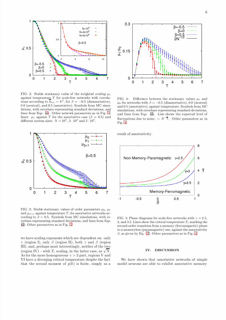
FIG. 2: Stable stationary value of the weighted overlap µ1against temperature T for scale-free networks with correla-tions according to knn ∼ kβ , for β = −0.5 (disassortative),0.0 (neutral), and 0.5 (assortative). Symbols from MC simu-lations, with errorbars representing standard deviations, and

lines from Eqs. (6). Other network parameters as in Fig. 1.Inset: µ1 against T for the assortative case (β = 0.5) anddifferent system sizes: N = 104, 3 · 104 and 5 · 104.

0

0.5

1

0 1 2 3 4 5 6 7

µ x

T

β=0.5

µ0µ1

µβ+1

FIG. 3: Stable stationary values of order parameters µ0, µ1and µβ+1 against temperature T , for assortative networks ac-cording to β = 0.5. Symbols from MC simulations, with er-rorbars representing standard deviations, and lines from Eqs.

(6). Other parameters as in Fig. 1.

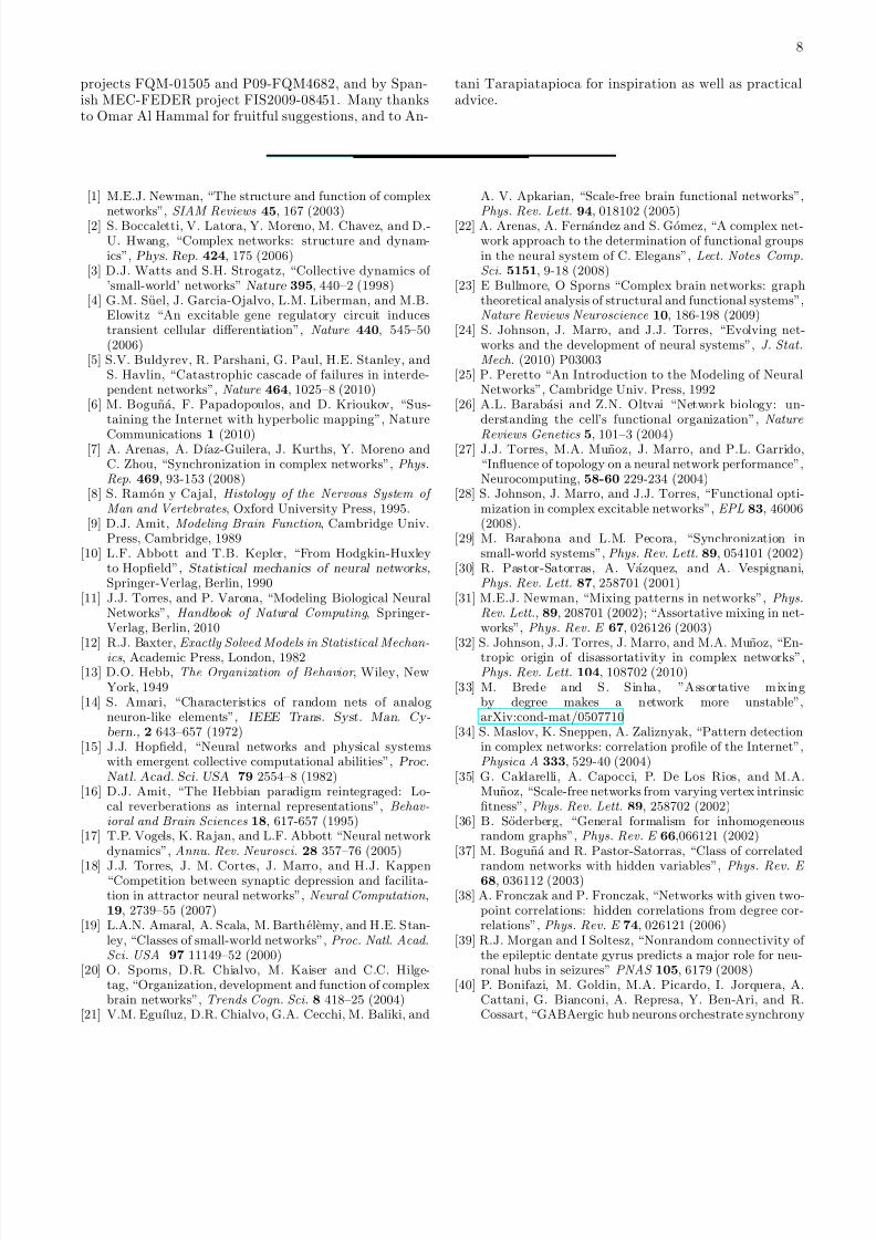
we have scaling exponents which are dependent on: onlyγ (region I), only β (region II), both γ and β (regionIII), and, perhaps most interestingly, neither of the two

(region IV) – with T c scaling, in the latter case, as√

N .As for the more homogeneous γ > 3 part, regions V andVI have a diverging critical temperature despite the factthat the second moment of p(k) is finite, simply as a

0

0.15

0.3

0 1 2 3 4 5 6 7

µ 1 - µ 0

T

β=-0.5β=0

β=0.52N

-1/2

FIG. 4: Difference between the stationary values µ1 andµ0 for networks with β = −0.5 (disassortative), 0.0 (neutral)and 0.5 (assortative), against temperature. Symbols from MCsimulations, with errorbars representing standard deviations,and lines from Eqs. (6). Line shows the expected level of

fluctuations due to noise, ∼ N −1

2 . Other parameters as inFig. 1.

result of assortativity.

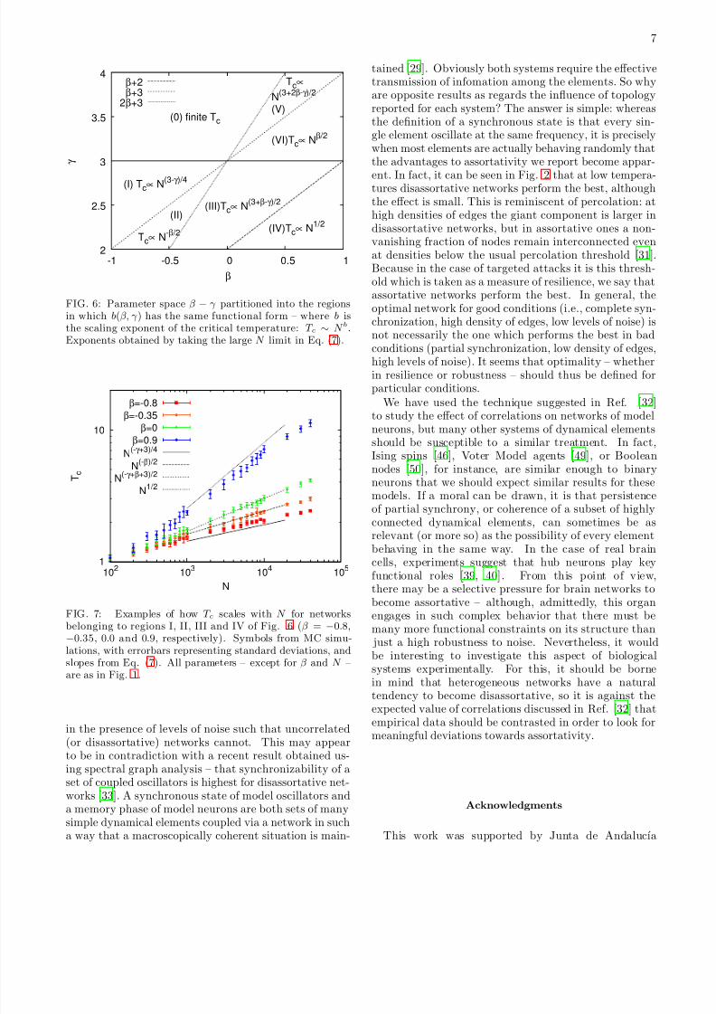
FIG. 5: Phase diagrams for scale-free networks with γ = 2.5,3, and 3.5. Lines show the critical temperature T c marking thesecond-order transition from a memory (ferromagnetic) phaseto a memoryless (paramagnetic) one, against the assortativityβ, as given by Eq. (7). Other parameters as in Fig. 1.

IV. DISCUSSION

We have shown that assortative networks of simplemodel neurons are able to exhibit associative memory



7

2

2.5

3

3.5

4

-1 -0.5 0 0.5 1

γ

β

(0) finite Tc

(I) Tc∝ N(3-γ )/4

(IV)Tc∝ N1/2

Tc∝ N-β /2

(II)(III)Tc∝ N

(3+β-γ )/2

(V)

Tc∝

N(3+2β-γ )/2

(VI)Tc∝ Nβ /2

β+2β+3

2β+3

FIG. 6: Parameter space β − γ partitioned into the regionsin which b(β, γ ) has the same functional form – where b isthe scaling exponent of the critical temperature: T c ∼ N b.Exponents obtained by taking the large N limit in Eq. (7).

1

10

102

103

104

105

T c

N

β=-0.8

β=-0.35

β=0

β=0.9

N(-γ +3)/4

N(-β)/2

N(-γ +β+3)/2

N1/2

FIG. 7: Examples of how T c scales with N for networksbelonging to regions I, II, III and IV of Fig. 6 (β = −0.8,−0.35, 0.0 and 0.9, respectively). Symbols from MC simu-lations, with errorbars representing standard deviations, andslopes from Eq. (7). All parameters – except for β and N –are as in Fig. 1.

in the presence of levels of noise such that uncorrelated(or disassortative) networks cannot. This may appearto be in contradiction with a recent result obtained us-ing spectral graph analysis – that synchronizability of aset of coupled oscillators is highest for disassortative net-works [33]. A synchronous state of model oscillators anda memory phase of model neurons are both sets of manysimple dynamical elements coupled via a network in sucha way that a macroscopically coherent situation is main-

tained [29]. Obviously both systems require the effectivetransmission of infomation among the elements. So whyare opposite results as regards the influence of topologyreported for each system? The answer is simple: whereasthe definition of a synchronous state is that every sin-gle element oscillate at the same frequency, it is preciselywhen most elements are actually behaving randomly thatthe advantages to assortativity we report become appar-

ent. In fact, it can be seen in Fig. 2 that at low tempera-tures disassortative networks perform the best, althoughthe effect is small. This is reminiscent of percolation: athigh densities of edges the giant component is larger indisassortative networks, but in assortative ones a non-vanishing fraction of nodes remain interconnected evenat densities below the usual percolation threshold [31].Because in the case of targeted attacks it is this thresh-old which is taken as a measure of resilience, we say thatassortative networks perform the best. In general, theoptimal network for good conditions (i.e., complete syn-chronization, high density of edges, low levels of noise) isnot necessarily the one which performs the best in badconditions (partial synchronization, low density of edges,high levels of noise). It seems that optimality – whetherin resilience or robustness – should thus be defined forparticular conditions.

We have used the technique suggested in Ref. [32]to study the effect of correlations on networks of modelneurons, but many other systems of dynamical elementsshould be susceptible to a similar treatment. In fact,Ising spins [46], Voter Model agents [49], or Booleannodes [50], for instance, are similar enough to binaryneurons that we should expect similar results for thesemodels. If a moral can be drawn, it is that persistenceof partial synchrony, or coherence of a subset of highlyconnected dynamical elements, can sometimes be as

relevant (or more so) as the possibility of every elementbehaving in the same way. In the case of real braincells, experiments suggest that hub neurons play keyfunctional roles [39, 40]. From this point of view,there may be a selective pressure for brain networks tobecome assortative – although, admittedly, this organengages in such complex behavior that there must bemany more functional constraints on its structure than

just a high robustness to noise. Nevertheless, it wouldbe interesting to investigate this aspect of biologicalsystems experimentally. For this, it should be bornein mind that heterogeneous networks have a naturaltendency to become disassortative, so it is against the

expected value of correlations discussed in Ref. [32] thatempirical data should be contrasted in order to look formeaningful deviations towards assortativity.

Acknowledgments

This work was supported by Junta de Andalucıa



8

projects FQM-01505 and P09-FQM4682, and by Span-ish MEC-FEDER project FIS2009-08451. Many thanksto Omar Al Hammal for fruitful suggestions, and to An-

tani Tarapiatapioca for inspiration as well as practicaladvice.

[1] M.E.J. Newman, “The structure and function of complex

networks”, SIAM Reviews 45, 167 (2003)[2] S. Boccaletti, V. Latora, Y. Moreno, M. Chavez, and D.-U. Hwang, “Complex networks: structure and dynam-ics”, Phys. Rep. 424, 175 (2006)

[3] D.J. Watts and S.H. Strogatz, “Collective dynamics of ’small-world’ networks” Nature 395, 440–2 (1998)

[4] G.M. Suel, J. Garcia-Ojalvo, L.M. Liberman, and M.B.Elowitz “An excitable gene regulatory circuit inducestransient cellular differentiation”, Nature 440, 545–50(2006)

[5] S.V. Buldyrev, R. Parshani, G. Paul, H.E. Stanley, andS. Havlin, “Catastrophic cascade of failures in interde-pendent networks”, Nature 464, 1025–8 (2010)

[6] M. Boguna, F. Papadopoulos, and D. Krioukov, “Sus-taining the Internet with hyperbolic mapping”, Nature

Communications 1 (2010)[7] A. Arenas, A. Dıaz-Guilera, J. Kurths, Y. Moreno and

C. Zhou, “Synchronization in complex networks”, Phys.Rep. 469, 93-153 (2008)

[8] S. Ramon y Cajal, Histology of the Nervous System of

Man and Vertebrates, Oxford University Press, 1995.[9] D.J. Amit, Modeling Brain Function , Cambridge Univ.

Press, Cambridge, 1989[10] L.F. Abbott and T.B. Kepler, “From Hodgkin-Huxley

to Hopfield”, Statistical mechanics of neural networks,Springer-Verlag, Berlin, 1990

[11] J.J. Torres, and P. Varona, “Modeling Biological NeuralNetworks”, Handbook of Natural Computing , Springer-Verlag, Berlin, 2010

[12] R.J. Baxter, Exactly Solved Models in Statistical Mechan-ics, Academic Press, London, 1982

[13] D.O. Hebb, The Organization of Behavior , Wiley, NewYork, 1949

[14] S. Amari, “Characteristics of random nets of analogneuron-like elements”, IEEE Trans. Syst. Man. Cy-bern., 2 643–657 (1972)

[15] J.J. Hopfield, “Neural networks and physical systemswith emergent collective computational abilities”, Proc.

Natl. Acad. Sci. USA 79 2554–8 (1982)[16] D.J. Amit, “The Hebbian paradigm reintegraged: Lo-

cal reverberations as internal representations”, Behav-ioral and Brain Sciences 18, 617-657 (1995)

[17] T.P. Vogels, K. Rajan, and L.F. Abbott “Neural networkdynamics”, Annu. Rev. Neurosci. 28 357–76 (2005)

[18] J.J. Torres, J. M. Cortes, J. Marro, and H.J. Kappen“Competition between synaptic depression and facilita-tion in attractor neural networks”, Neural Computation ,19, 2739–55 (2007)

[19] L.A.N. Amaral, A. Scala, M. Barthelemy, and H.E. Stan-ley, “Classes of small-world networks”, Proc. Natl. Acad.Sci. USA 97 11149–52 (2000)

[20] O. Sporns, D.R. Chialvo, M. Kaiser and C.C. Hilge-tag, “Organization, development and function of complexbrain networks”, Trends Cogn. Sci. 8 418–25 (2004)

[21] V.M. Eguıluz, D.R. Chialvo, G.A. Cecchi, M. Baliki, and

A. V. Apkarian, “Scale-free brain functional networks”,

Phys. Rev. Lett. 94, 018102 (2005)[22] A. Arenas, A. Fernandez and S. Gomez, “A complex net-work approach to the determination of functional groupsin the neural system of C. Elegans”, Lect. Notes Comp.Sci. 5151, 9-18 (2008)

[23] E Bullmore, O Sporns “Complex brain networks: graphtheoretical analysis of structural and functional systems”,Nature Reviews Neuroscience 10, 186-198 (2009)

[24] S. Johnson, J. Marro, and J.J. Torres, “Evolving net-works and the development of neural systems”, J. Stat.Mech. (2010) P03003

[25] P. Peretto “An Introduction to the Modeling of NeuralNetworks”, Cambridge Univ. Press, 1992

[26] A.L. Barabasi and Z.N. Oltvai “Network biology: un-derstanding the cell’s functional organization”, Nature

Reviews Genetics 5, 101–3 (2004)[27] J.J. Torres, M.A. Munoz, J. Marro, and P.L. Garrido,

“Influence of topology on a neural network performance”,Neurocomputing, 58-60 229-234 (2004)

[28] S. Johnson, J. Marro, and J.J. Torres, “Functional opti-mization in complex excitable networks”, EPL 83, 46006(2008).

[29] M. Barahona and L.M. Pecora, “Synchronization insmall-world systems”, Phys. Rev. Lett. 89, 054101 (2002)

[30] R. Pastor-Satorras, A. Vazquez, and A. Vespignani,Phys. Rev. Lett. 87, 258701 (2001)

[31] M.E.J. Newman, “Mixing patterns in networks”, Phys.Rev. Lett., 89, 208701 (2002); “Assortative mixing in net-works”, Phys. Rev. E 67, 026126 (2003)

[32] S. Johnson, J.J. Torres, J. Marro, and M.A. Munoz, “En-tropic origin of disassortativity in complex networks”,Phys. Rev. Lett. 104, 108702 (2010)

[33] M. Brede and S. Sinha, ”Assortative mixingby degree makes a network more unstable”,arXiv:cond-mat/0507710

[34] S. Maslov, K. Sneppen, A. Zaliznyak, “Pattern detectionin complex networks: correlation profile of the Internet”,Physica A 333, 529-40 (2004)

[35] G. Caldarelli, A. Capocci, P. De Los Rios, and M.A.Munoz, “Scale-free networks from varying vertex intrinsicfitness”, Phys. Rev. Lett. 89, 258702 (2002)

[36] B. Soderberg, “General formalism for inhomogeneousrandom graphs”, Phys. Rev. E 66,066121 (2002)

[37] M. Boguna and R. Pastor-Satorras, “Class of correlated

random networks with hidden variables”, Phys. Rev. E 68, 036112 (2003)

[38] A. Fronczak and P. Fronczak, “Networks with given two-point correlations: hidden correlations from degree cor-relations”, Phys. Rev. E 74, 026121 (2006)

[39] R.J. Morgan and I Soltesz, “Nonrandom connectivity of the epileptic dentate gyrus predicts a major role for neu-ronal hubs in seizures” PNAS 105, 6179 (2008)

[40] P. Bonifazi, M. Goldin, M.A. Picardo, I. Jorquera, A.Cattani, G. Bianconi, A. Represa, Y. Ben-Ari, and R.Cossart, “GABAergic hub neurons orchestrate synchrony

http://arxiv.org/abs/cond-mat/0507710

http://arxiv.org/abs/cond-mat/0507710



9

in developing hippocampal networks”, Science 326, 1419(2009)

[41] O. Paulsen and T.J. Sejnowski, “Natural patterns of ac-tivity and long-term synaptic plasticity”, Curr. Opin.

Neurobiol. 10 172–9 (2000)[42] A. Gruart, M.D. Munoz, and J.M. Delgado-Garcıa, “In-

volvement of the CA3-CA1 synapse in the acquisition of associative learning in behaving mice”, J. Neurosci. 26,1077–87 (2006).

[43] In directed networks the mean in degree and the meanout degree necessarily coincide, whatever the forms of thein and out distributions.

[44] As in statistical physics, one can consider the micro-canonical ensemble, in which each element (network) sat-isfies the constraints exactly, or the canonical ensem-ble, where the constraints are satisfied on average [45].Throughout this work, we shall refer to canonical ensem-

bles.[45] G. Bianconi, “Entropy of network ensembles”, Phys. Rev.

E 79, 036114 (2009)[46] G. Bianconi, “Mean-field solution of the Ising model on a

BarabsiAlbert network”, Phys. Lett. A 303 166–8 (2002)[47] S.N. Dorogovtsev, A.L. Ferreira, A.V. Goltsev, and

J.F.F. Mendes, “Zero pearson coefficient for strongly cor-related growing trees”, Phys. Rev. E 81, 031135 (2010)

[48] G. Bianconi, “The entropy of randomized network en-

sembles”, Europhys. Lett. 81, 28005 (2008)[49] K. Suchecki, V.M. Eguıluz, and M. San Miguel “Conser-

vation laws for the voter model in complex networks”,EPL, 69 , 228–34 (2005)

[50] T.P. Peixoto, “Redundancy and error resilience inBoolean Networks”, Phys. Rev. Lett. 104, 048701 (2010)

enhancing neural-network performance via assortativity

Documents