Philosophiae Doctor (PhD)Thesis 2016:62

Wei Liu

Enhancement of Coagulant Dosing Control in Water and Wastewater Treatment Processes

Forbedring av koagulant-doseringskontroll i renseprosesser for vann og avløp

Philosophiae Doctor (PhD

), Thesis 2016:62W

ei Liu

Norwegian University of Life Sciences Faculty of Environmental Science and TechnologyDepartment of Mathematical Sciences and Technology (IMT)

ISBN: 978-82-575-1382-5 ISSN: 1894-6402

Postboks 5003 NO-1432 Ås, Norway+47 67 23 00 00www.nmbu.no

Enhancement of Coagulant Dosing Control in Water and Wastewater Treatment Processes

Supervisory team Harsha Ratnaweera, Professor (main supervisor) Department of Mathematical Sciences and Technology Norwegian University of Life Sciences Arve Heistad, Associate Professor (co-supervisor) Department of Mathematical Sciences and Technology Norwegian University of Life Sciences Evaluation committee Joachim Fettig, Professor (first opponent) Department of Environmental Engineering and Applied Informatics University of Applied Sciences Ostwestfalen-Lippe, Hoexter, Germany Torleiv Bilstad, Professor (second opponent) Department of Mathematics and Science University of Stavanger, Norway Volha Shapaval, Associate Professor (committee coordinator) Department of Mathematical Sciences and Technology Norwegian University of Life Sciences

Summary

Chemical coagulation is one of the most important treatment processes in wastewater

treatment and drinking water treatment. Defining the optimal coagulant dosage is a vital operation

that decides the treatment efficiency and economy of the coagulation process. Chemical

coagulation is a well-defined process where the optimal coagulant dosage is dependent on the

influent quality, expressed by particle concentration, pH, temperature, colour or phosphate,

alkalinity, etc. However, no conceptual model has been developed due to the complexity of this

process and the research on coagulant dosage control has continued for decades (Ratnaweera and

Fettig, 2015). Among all the avenues of research, the model predictive control based on online

measurements is the most promising concept for coagulant dosage control. It presents various

methods of model calibration and well-defined testing procedures. A Feed-Forward (FF) model

based concept of a multi-parameter dosing control system for wastewater was originally proposed

by Ratnaweera et al. (1994) and then improved upon by Lu (2003) and Rathnaweera (2010).

According to previous results of full-scale tests, the multi-parameter dosing control system has

proven to provide acceptable effluent quality and improved economy on most occasions in several

wastewater treatment plants.

The multi-parameter dosing control system relies on many online instruments and

empirical models. Generally, there are four aspects challenging the performance and utilization of

the system. Firstly, it is necessary for the empirical model to prove universality of utilization,

which refers to the independence of diverse water sources and process dynamics. Secondly, the

performance of such a system is challenged by abnormal inlet variation. Heavy rain particularly

requires improvements of the model’s capacity of dosage prediction. Thirdly, different

requirements of treatment results should be met by the system, which needs to realise flexibility

of utilization with other treatment processes in both full-scale wastewater and drinking water

treatment. Fourthly, the model performance of real-time dosage control highly depends on data

accuracy of online measurements and therefore demands efficient error detection of said online

measurements. Hence, based on the existing multi-parameter dosing control system, this thesis

approaches the aforementioned challenges and improves upon the existing system by pursuing

full-scale tests and solutions.

ii

Drinking water treatment is one of the major application fields for the coagulation process.

This thesis extends the multi-parameter dosing control system originally developed for wastewater

treatment to drinking water treatment. The testing results show that the system provides more even

effluent results than flow-proportional dosing, and saves as much as 10 % coagulant consumption.

In view of control strategy, a feedback (FB) with outlet qualities is identified as a critical

factor for system improvement. It is especially applicable to managing extreme inlet variations

such as heavy rains, and also to achieve required outlet qualities presented by users. Thus, the

inclusion of an outlet turbidity and a set point combined with the existing feed-forward (FF) model

will improve the results. The testing results show that the model capacity improves by the dosage

adjustment of the feedforward-feedback (FB-FF) model, ranging from 66 % to 197 % of the FF

model. Consequently, related outlet quality can be more stable than the FF model, alongside

coagulant consumption showing further reductions in the range of 3.7 %-15.5 %.

Utilization of the FF-FB model is limited because the outlet sensor is always several hours

delayed in providing feedback information, due to the long hydraulic retention time of common

sedimentation tanks. Hence, this thesis proposes the development of an outlet software sensor

based on inlet sensors and the dosage. The software sensor can predict outlet turbidity before

coagulated water goes through the sedimentation tank, which serves as a timely feedback for

defining optimal dosage. The testing results show that the software sensor performs well within

the main working range.

Reliability of the FF-FB model is highly dependent on the operative status of online

instruments, which can fault and become out-of-order. In order to estimate and detect the potential

measurement errors this thesis proposes a model-based measurement error detection. According

to the testing results, the proposed detection method has a better efficiency to detect the

measurement errors than a traditional method (the normal variation range checking).

Consequently, the FB-FF model is enabled to work with accurate measurements of online

instruments.

In conclusion, the applicability of an automated dosing control system for drinking water

treatment and a concept to improve the system with the use of a FB-FF model is proposed. A

software sensor for outlet turbidity is proposed to enable the FB model. Since all control systems

iii

based on online measurements are critically dependent on the measurement accuracies, a new

concept to validate the measurement is proposed.

iv

Sammendrag

Kjemisk felling er en av de viktigste enhetsprosessene i både avløps- og

drikkevannsbehandling. Identifisering av optimal koagulantdose er sentralt i driften av

koaguleringsprosessen, og avgjørende for både rensegraden og driftsøkonomien i prosessen.

Kjemisk felling er en veldefinert prosess der den optimale koagulantdosen avhenger av kvaliteten

på innkommende vann, gitt ved partikkelkonsentrasjon, pH, temperatur, farge eller fosfatinnhold,

alkalinitet osv. Det finnes imidlertid ingen universielle konseptuell modell for å bestemme optimal

dose ettersom prosessen er svært kompleks. Dette har ført til årtier med forskning på regulering av

koagulantdosen (Ratnaweera og Fettig, 2015). Av de ulike forskningsretningene har prediktiv

regulering basert på online målinger vist seg svært populært, og inkluderer forskjellige metoder

for modellkalibrering og definerte testprosedyrer. Et konsept bestående av multi-parameter

doseringsregulering for avløpsrensing ble opprinnelig foreslått av Ratnaweera et al. (1994) og

forbedret av Lu (2003) og Rathnaweera (2010). Tidligere fullskala tester har vist at systemet for

multi-parameter doseringsregulering gir akseptabel kvalitet på behandlet vann og forbedret

driftsøkonomi i et antall avløpsbehandlingsanlegg.

Systemet for multi-parameter doseringsregulering avhenger av online målinger fra mange

instrumenter, samt empiriske modeller. Generelt kan det identifiseres fire aspekter som utfordrer

funksjonen og nytten til systemet. For det første må det demonstreres at den empiriske modellen

er universelt nyttig, dvs. at den fungerer uavhengig av hvilken vanntype og prosessdynamikk man

har. For det andre blir systemet utfordret av unormale variasjoner i innløpet, spesielt ved større

nedbørshendelser, noe som krever utvidet modellkapasitet. For det tredje må systemet kunne

oppfylle varierende lokale krav til rensegrad, noe som krever fleksibilitet når det gjelder bruk i

ulike behandlingsprosesser i både avløps- og drikkevannsbehandling. For det fjerde avhenger

funksjonen til sanntids doseringssystemer i stor grad av nøyaktigheten til online instrumenter, noe

som krever et effektivt system for å avdekke feil i målingene. Med utgangspunkt i det eksisterende

multi-parameter doseringssystemet vil avhandlingen ta tak i de ovenstående utfordringene og

forbedre systemet basert på testing og verktøy i fullskala.

Drikkevannsbehandling er et av de viktige anvendelsesområdene for kjemisk felling.

Denne avhandlingen utvider systemet for multi-parameter doseringsregulering, i utgangspunktet

utviklet for avløpsrensing, til drikkevannsbehandling. Testresultatene viser at systemet ga mer

v

stabil utløpskvalitet enn mengdeproporsjonal dosering og ga opptil 10 % besparelse i

koagulantforbruk.

Når det gjelder reguleringsstrategi, ble det benyttet en tilbakekobling (Feed Back, FB) som

inkluderte utløpsturbiditet og en skal-verdi i kombinasjon med den eksisterende modellen basert

på foroverkobling (Feed Forward, FF), som tar sikte på å håndtere unormal variasjon i innløpet,

spesielt ved tung nedbør, og samtidig oppnå brukerens ønskede utløpskvalitet. Testresultatene

viser at modellens kapasitet forbedres gjennom dosejusteringene til modellen basert på

foroverkobling-tilbakekobling (FF-FB), fra 66 % til 197 % av modellen basert på kun

foroverkobling. Det medfører at den tilhørende utløpskvaliteten kan holdes mer stabil. Samtidig

påvises det at koagulantforbruket ytterligere reduseres med 3.7 %-15.5 %.

Utnyttelsen av modellen basert på foroverkobling-tilbakekobling (FF-FB) begrenses av det

forhold at utløpssensoren alltid gir flere timers forsinket tilbakemelding på grunn av lange

hydrauliske oppholdstider i typiske sedimenteringbassenger. I denne avhandlingen ble det derfor

utviklet en soft-sensor basert på innløpssensorene og doseringsnivået. Soft-sensoren kan forutsi

utløpsturbiditeten før koagulert vann passerer sedimenteringstanken og kan derfor gi rettidig

tilbakemelding for å bestemme optimal dosering. Test-resultatene viser at soft-sensoren fungerte

godt innenfor det primære arbeidsområdet.

Påliteligheten til modellen basert på foroverkobling-tilbakekobling er svært avhengig av

driftsstatusen til online instrumenter. For å kunne detektere og estimere mulige feil i målingene,

ble det i denne avhandlingen utviklet et modellbasert system for feildetektering. Ifølge

testresultatene detekterer det foreslåtte systemet feil mer effektivt enn en tradisjonell metode (sjekk

basert på variasjon innenfor normalområdet), noe som gjør det mulig for modellen basert på

foroverkobling-tilbakekobling å arbeide med nøyaktige målinger fra online instrumenter.

Konkluderende foreslår tesen anvendelse av et automatisert doseringsstyresystem for

drikkevannbehandling, samt et konsept for å forbedre systemet med bruk av en FB-FF-modell. En

myksensor for utløp turbiditet foreslås for å muliggjøre anvendelse av en FB modell. Da alle

styresystemer basert på elektroniske målinger er kritisk avhengige av målenøyaktigheter, er et nytt

konsept for å validere målingen foreslått.

vi

Acknowledgements First of all, I would like to present my profound gratitude to my main supervisor prof.

Harsha Ratnaweera, for making me the world of water treatment accessible, offering me scientific

guidance and providing the opportunity to gain comprehensive knowledge. In addition, I deeply

appreciate his trust, patience and inspiration during my whole PhD period.

Sincere thanks are extended to Mr. Song Heping for his communication with wastewater

and drinking water treatment plants, which were highly supportive to my field work. I present my

great thanks to Mr Jiang Yuejie from Haining No.2 DWTP and Mr Ma Xuefan from Haining

Salcon DWTP, for their valuable support during my experiments.

I am glad to express my deep thanks to Mr Dejan Josik from INDAS Co Ltd., Serbia for

his professional assistance to develop the CDCS software and signal communication, alongside

his valuable online support.

I would like to show my deep gratitude to prof. Knut Kvaal for his guidance, knowledge

and advices on statistics and modelling.

I highly appreciate DOSCON AS, Norway, for offering hardware support - the Coagulant

Dosage Control System - and for funding my research. Without generous funding from DOSCON

AS it would not have been possible to complete my PhD research.

I am honoured to express my deep gratitude to the supervisor of my Master’s degree prof.

Li Yawei, for his recommendation of my PhD application as well as his great encouragements.

I am happy to offer thanks to my fellow PhD candidates Lelum Manamperuma, Pavlo

Kozminykh, Vegard Nilsen, Nataliia Sivchenko, Duo Zhang and Xiaodong Wang for every

discussion and help shared during our PhD lives. I would like to offer my thanks to Vegard again

for the translation of the summary of this thesis.

It is an honour for me to convey my appreciation to the Norwegian University of Life

Science (NMBU) and Department of Mathematical Sciences and Technology (IMT) for providing

me a rigorous course of study.

I offer my heartiest thanks to my parents and grandparents for their unlimited support,

which provided me with great confidence in pursuing my PhD. I am deeply thankful to my loving

wife Wenmin for her endless support, patience and understanding.

LIST OF ACRONYMS

LIST OF FIGURES

LISTOF TABLES

Table 1. Normal measurement range of each parameter. Table 2. Statistical results of experimental line and conventional line in N2DWTP. Table 3. Parameters of changes on coagulant consumption in Haining N2DWTP. Table 4. Parameters of changes on coagulant consumption in NRA WWTP. Table 5. Plug flow TUO simulation under the different distribution ratio.

Figure 1. Research framework of this thesis. Figure 2. Overview of Haining Number two DWT plant. Figure 3. Schematic of treatment process in N2DWTP. Figure 4. Inlet online instruments of N2DWTP. Figure 5. Overview of Haining Salcon DWT plant. Figure 6. Schematic of treatment process in SDWTP. Figure 7. Inlet online instruments of SDWTP. Figure 8. Schematic of treatment process in NRA WWTP. Figure 9. Inlet online instruments of NRA WWTP. Figure 10. Profile of the Coagulant dosage control system. Figure 11. Setting interface of variation validation. Figure 12. Setting interface of normal measurement range. Figure 13. The procedure of full-scale tests. Figure 14. Comparison of conventional dosing and modelled experimental dosing at

N2DWTP in stage of passive test. Figure 15. Comparison of conventional dosing and modelled experimental dosing at the

Salcon DWTP. Figure 16. Large variation of outlet turbidity during storms in active tests of N2DWTP. Figure 17. Large variation of outlet turbidity during wet weather in active tests of NRA

WWTP. Figure 18. Control strategy of combining feedforward and feedback. Figure 19. Statistics on passive test of the FF-FB model in N2DWTP. Figure 20. Statistics on passive test of the FF-FB model in NRA WWTP. Figure 21. Significance of mixing effect under different mixing percentage. Figure 22. Concept of the TUO software-sensor. Figure 23. Correlation between shifted TUO and TUO prediction. Figure 24. Concept of error detection of inlet measurements. Figure 25. Detection criterion of inlet measurement errors. Figure 26. Comparison of proposed detection method and the traditional method.

Contents 1. INTRODUCTION

1.1 Coagulant dosage control in practice

1.2 Developments in coagulant dosage control

1.3 Need for improvements in coagulation practice

1.3.1 Universality

1.3.2 Model capacity of coagulant dosage control

1.3.3 Flexibility of utilization

1.3.4 Data quality of online measurements

1.4 Research objectives

EXPERIMENTAL METHODS AND PROCEDURES

2.1 Introduction of full-scale processes

2.1.1 Haining Number two DWTP

2.1.2 Haining Salcon DWTP

2.1.3 Nedre Romerike WWTP

2.2 Introduction of hardware of the CDCS

2.3 Data preprocessing for model calibration

2.3.1 Matching outlet data with inlet

2.3.2 Measurement error elimination

2.4 Model calibration

2.5 Current online detection of measurement errors

3. RESULTS AND DISCUSSION

3.1 Testing the universality of the CDCS

3.1.1 Procedure of full-scale tests

3.1.2 Results of passive tests

3.1.3 Results of active tests

3.1.4 Dosage control during storms

3.1.5 Universality analysis of the CDCS

3.2 Improvement of model capacity

3.2.1 Concept of combining feedforward and feedback model

3.2.2 Validation of the FF-FB model

3.2.3 Effect on coagulant consumption

3.2.4 Improvement effect on the flexibility

ii

3.2.5 Limitation of the FF-FB model

3.3 Preconditions of TUO software sensor development

3.3.1 Definition of plug flow TUO

3.3.2 Simulation results of plug flow TUO

3.4 Development of TUO software Sensor

3.4.1 Concept of TUO software sensor

3.4.2 Testing of TUO software sensor

3.5 Improvement on error detection of inlet measurements

3.5.1 Concept of the detection method

3.5.2 Detecting criterion of inlet measurement errors

3.5.3 Comparison between the new method and the current method of error detection

3.6 Shorter period of the data collection

4. CONCLUSIONS

5. RECOMMENDATIONS FOR FURTHER STUDIES

6. REFERENCES

7. APENDIX-PUBLICATIONS

7.1 Better treatment efficiencies and process economics with real-time coagulant dosing control

7.2 Improvement of multi-parameter based Feed-Forward coagulant dosing control systems with Feed-Back functionalities

7.3 Feed-forward based software sensor for outlet turbidity of coagulation process

7.4 Model based measurement error estimation of coagulant dosage control system

1

1. INTRODUCTION

Chemical coagulation has been widely used in wastewater treatment plants (WWTP)

for the removal of particulate matter and phosphates, and in drinking water treatment plants

(DWTP) for the removal of particulate matter and Natural Organic matter (NOM) (AWWA,

2011). Considerable fractions of chemical oxygen demand (COD), total phosphorus (TP) and

NOM are found in particulate or colloidal fractions, thus can be highly reduced by a coagulation

process (Guida et al., 2007; Shutova et al., 2014). The removal process may occur according to

all four coagulation mechanisms, i.e. neutralizing charge on particles, compressing double

layers of charged particles, bridging particles together and by sweeping of flocs. These

coagulated particulate matters are in a stage of destabilization and increased size after

coagulation, and hence can be separated from liquid (Tchobanoglous et al., 1997). Furthermore,

dissolved phosphates (P) as a pollutant can be removed after reacting with a metal coagulant

and converting into particulate form, or by adsorption on to the other coagulated species.

A coagulation treatment process physically consists of coagulant dosing pumps, rapid

mixing units, flocculation chambers, and flocs separation units such as sedimentation tanks,

filtration and flotation systems. During the coagulation process, certain amount of coagulant is

dosed into raw water primarily leading to the growth of flocs in flocculation chambers under

the slow mixing. Finally particles with suitable size are separated.

Coagulation treatment plays an important role in water and wastewater treatment

because of several reasons. Firstly, the coagulation treatment has high efficiency of particles,

NOM and phosphate removal. Secondly, a full-scale coagulation process can be simply

operated through few control parameters (e.g. coagulant dosage). Thirdly, coagulation has a

short physical footprint of treatment process that in turn requires less land usage. Fourthly, in

order to meet various treatment requirements, a coagulation process is flexible to work with

other treatment processes, for example three combinations with biological treatment: pre-

precipitation, simultaneous precipitation and post-precipitation (Tchobanoglous et al., 1997).

Fifthly, less energy consumption and high tolerance of variations of treatment load are other

notable advantages of a coagulation process (Ratnaweera et al., 2002). Therefore, coagulation

is a competitive treatment process in both DWTP and WWTP.

2

1.1 Coagulant dosage control in practice

The optimal coagulant dosage is the least amount of coagulants required to achieve the

anticipated treated water quality. Based on coagulation mechanisms, the optimal coagulant

dosage depends on raw water quality such as particle concentration, pH, alkalinity, hardness,

temperature, phosphate concentration (in wastewater treatment), NOM (in drinking water),

ionic strength, etc. (Ratnaweera, 1991; Maier et al., 2004; Rathnaweera, 2010). Treated water

quality is the result of these parameters, features of the separation stage and coagulant dosage.

In laboratory, jar tests as the most common method are widely used for defining the optimal

dosage for a given water quality. However, it becomes time-consuming and impractical to deal

with rapid variation of the inlet water quality in full-scale treatment (Joo et al., 2000; Yu et al.,

2000). Ratnaweera (2004) pointed out that water quality varies frequently in WWT, which

could require a change in optimal dosages even within 15 minutes. Thus, it is necessary to

define the optimal dosage for the incoming water in real-time and automatically.

It is difficult to control coagulant dosage in full-scale treatment plants. Ratnaweera and

Fettig (2015) pointed out that universally accepted mathematical descriptions are still not

available for the coagulation process because of the complexities presented within the

coagulation process. Since influencing parameters are not changing proportionally, it is

impossible to simplify the relationship by replacing one parameter with others (Guo et al., 2009)

or by using one parameter for comprehensive coagulation control (Ratnaweera et al., 2005), if

one wants to run the process optimally and economically. Similar to most industrial processes,

the water quality of treated water can be used as FB for dosage adjustment, without having

much insight to the process dynamics. However, it is difficult to achieve in full-scale water and

wastewater treatment because of hours long retention time of sedimentation tanks, combined

with rapid change inlet qualities (Ratnaweera, 2004). Therefore, a number of researchers have

been focusing on coagulant dosage control – both on conceptual and empirical models, based

on inlet qualities (Dentel, 1991; Joo, et al., 2000; Baxter et al., 2001; Maier, 2004; Ratnaweera

et al., 2005; Rathnaweera, 2010).

Outlet particles and P concentration (if WWT), as the results of influence parameters

and dosage, are key control targets of the full-scale coagulation process. As the main operating

parameter, dosage should be controlled well to meet the effluent requirement.

In a coagulant dosing control system, it is important to involve user inputs to achieve

different outlet requirements. Since the coagulation process often works before other treatment

processes, the outlet quality should meet with requirements of the subsequent process. For

3

instance, too low P concentration or/and too low pH in the coagulation outlet could cause poor

performance in subsequent biological processes. This is because P is an essential element of

organism growth. Furthermore, according to the latest Norwegian regulation for WWTP,

overflow and bypass at the WWTP shall be included in the reporting of discharges. The WWTP

must achieve overall 94 % of total-P removal, and that cannot be achieved without over 96 %

of total-P removal of the portion which goes through the WWTP, so the annual average values

will be within the acceptable levels. For DWTP, outlet particle concentration of the coagulation

process can decide backwash frequency of downstream filtration treatment. Therefore, outlet

requirements of the coagulation processes are variable with different treatment plants and

dosage control should adapt to the different outlet requirements.

Dosage control also relates to operational cost, health and other issues. It is reported that

chemical cost could be up to 20 % of total operational cost (Hangouet et al., 2007), and some

reports show that the total operational cost is more or less equal to the cost of coagulant (VA

Support, 2012). Furthermore, Siriprapha et al. (2011) pointed out that the coagulation-

flocculation process usually generates large quantities of chemical sludge and Ødegaard (2009)

presented calculations for the sludge production in coagulation plants in Norway. Thus,

overdosage could yield unnecessarily high amounts of sludge, which leads to additional cost of

sludge treatment. There is also a concern on using coagulated sludge as fertilizer, as the plant

availability of phosphates. The overdosage results in stronger metal-P bond, which decreases

plant availability of P and reduces the benefit of the coagulated sludge accordingly

(Manamperuma et al., 2015). Furthermore, low pH in treated water resulted from overdosage

creates increased potential for corrosion in water transport systems. Maier et al. (2004) pointed

out that coagulation in drinking water treatment provides one of multiple barriers to protect

public health. The optimal dosage can significantly contribute to remove microorganisms and

hence reduce water borne illness among consumers.

1.2 Developments in coagulant dosage control

Researches on coagulant dosage control have been implemented for several decades.

Along with the development of online instruments and understanding of coagulation process,

methods of coagulant dosage control is being upgraded gradually (Jeppsson et al., 2002;

Vanrolleghem and Lee, 2003; Ratnaweera and Fettig, 2015). According to Schlenger et al.

(1996), process control can be classified into three stages: supervisory control, automatic

control and advanced control.

4

Flow-proportional and time-proportional dosage are two simplified methods. Namely,

coagulant feeding flow is proportional to incoming water flow and time. A survey among

Norwegian treatment plants indicated that over 80 % of DWTPs and WWTPs use flow

proportional, with or without over steering of pH, dosing control (Ratnaweera, 2004).

According to both outlet quality and results of jar tests, operators have to adjust the proportional

ratio regularly (Dentel, 1991). This scheme belongs to the supervisory control. Baxter et al.

(2002) pointed out that operators need to consider the results of jar tests and implement

corresponding operations. This scheme is suitable for raw water with relatively constant quality,

such as lake and reservoir as water source of DWTP. However, Ratnaweera and Fettig (2015)

points out that such a control scheme is not suited for real-time control of a continuous process,

especially when the raw water quality varies over a short period of time with considerable

amplitude.

In order to assist the flow-proportional dosage control, Stumm and O’Melia (1968) built

up a control chart to illustrate how the destabilization of particulate matter is decided by both

dosage and initial particle concentration. The control chart is helpful for operators to understand

the definition of an optimal dosage. A diagram of coagulation domain, initially developed by

Amirtharajah and Mills (1982), addresses that domination of each coagulation mechanism

(charge neutralization, double layers compression, bringing and sweep flocs) depends on

coagulation pH and dosage.

Based on DLVO theory (named after Derjaguin, Landau, Verwey and Overbeek), there

is an attractive force and a repulsive force between two particles that generates an energy barrier

when these two particles approach each other (Stumm and Morgan, 1995). Consequently,

particles naturally stabilize and disperse in water (Hunter, 2001). Feeding metal-iron coagulant

is the most common solution to destabilize particles, where charge neutralization is the

predominant mechanism (Amirtharajah and Mills, 1982). In order to indicate the degree of

charge neutralization, a streaming current detector (SCD) is able to provide an important

reference (Dentel et al., 1989). SCD can work online to evaluate whether dosage is adequate to

destabilize particles. SCD enables FB control through simple algorithms or linear models

(Walker et al., 1996; Baxter et al., 2002; Adgar et al., 2005; Oh and Lee, 2005). Based on

Henry’s Equation, zeta potential analyzer is able to indirectly detect net charges of particles

(Hunter, 1981; Sharp and Norris, 2015). It is often reported that SCD readings have a linear

relationship with zeta potential measurements (Ratnaweera and Fettig, 2015). However,

application of these electro-kinetic approaches are limited, because it proves to be useful mainly

5

when charge neutralization mechanism predominates (Stanly et al., 2000). Dentel (1995)

pointed out that the output of SCD sometimes exhibits a contradictory result for the coagulation

activation, because both surface charge of particles and charged functional groups on NOM

molecules are affected by pH. Consequently, although streaming current detectors are available

from a number of suppliers, there has been no standard calibration procedure so far (Ratnaweera

and Fettig, 2015).

Considering the complex physical dynamics and relationship between influence

parameters and dosage, model predictive control (MPC) relying on multiple online

measurements has been extensively studied and applied in full-scale coagulant dosage control

(Baxter et al., 1999; Yu et al., 2000; Zeng et al., 2003; Hamed et al., 2004; Ratnaweera et al.,

2005; Yu et al., 2011). As advanced control, MPC is more suitable for operating non-linear

multivariate system than experienced operators (AlGhazzawi and Lennox, 2009). Since the

conceptual model derived from chemical and physical features of coagulation process is still

not available, MPC of coagulant dosage has been carried out by empirical models so far

(Rietveld and Dudley, 2006; Maier et al., 2010; Ratnaweera and Fettig, 2015). Instead of

including all relevant influence parameters and knowing the dynamics of the physical process,

the empirical models are able to establish the relationship between a few online instruments and

dosage (Zeng et al., 2003; Maier et al., 2004). The empirical model can be classified into two

approaches: multivariate statistics and artificial intelligence (AI), both of which are driven by a

large number of historical data (Bloch and Denoeux, 2003; Fortuna et al., 2007). There are

many modelling methods belonging to these two approaches. Multivariate statistics approach

includes principle component regression (PCR), multiple linear regression (MLR), partial least

squares regression (PLSR), etc., whereas AI approach contains artificial neural networks

(ANN), expert system, fuzzy logic and genetic algorithms (Dellana and West, 2009). MPC

relies on the empirical model to become increasingly popular in coagulant dosage control.

Zhang and Stanley (1999) pointed out that it is difficult to realize coagulant dosage

control by traditional methods because of complex physical and chemical phenomena included

in the coagulation, flocculation and separation process. Whereas ANN as a proposed method

can overcome the complexities and predict the optimal dosage. The authors calibrated an ANN

model with 2 000 sets of operational data of a DWTP. The authors also suggest that the

proposed approach can be used for other DWTP after minor modification. Later, Stanley et al.

(2000) reported that the ANN model proved to be a useful method to predict coagulant dosage,

concluded from test results at two DWTPs.

6

Because empirical models are derived from historical data, data quality is a key factor

for the model performance. Joo et al. (2000) proved that data preprocessing is able to enhance

the performance of ANN models. Hence, the paper specified a procedure of the data

preprocessing. Input parameters of the model include temperature, pH, turbidity, and alkalinity.

Root mean square error (RMSE) is suggested as an indicator of model performance. Notably,

during rainy days especially in July and August, the authors point out that it is very difficult for

process operators to cope with the rapid fluctuation of inlet quality.

During the rainy season, Yu et al. (2000) observe that rapid change of inlet water quality

is a challenge for coagulant dosage control of DWT. The paper points out that daily data are

not adequate for model calibration, which could miss information of inlet quality. Hence, water

quality recorded every 15 minutes are used for the model calibration. Four online measurements

including inlet turbidity, inlet pH, inlet conductivity and outlet turbidity of settling tank are used

for inputs in the ANN model. Because an outlet parameter is involved into dosage prediction,

the model contains both FB and FF parameters. The best result of coefficient determination

(R2=0.97, an indicator of model performance) indicates that the dataset fits the model well.

Furthermore, the authors discover that a nonlinear model has better prediction results than a

linear model.

Pilot-scale tests of coagulant dosage control were carried out by Baxter et al. (2002).

Three-month operational data include temperature, particle counts, color, alkalinity, pH,

hardness, water flow, outlet turbidity and dosage. These pilot-scale tests proved that the ANN

model is able to achieve real-time dosage control based on online instruments. Because of the

pilot-scale tests, the authors highlights that the ANN model is able to cope with different

selected water flows. Moreover, the paper also illustrates that multiple models can be used for

achieving different user identified effluent targets. Further full-scale tests are highly suggested

by this paper.

Another notable pilot-scale test is carried out by Bloch and Denoeux (2003). The paper

demonstrates that the ANN model is an efficient tool for coagulant dosage control of DWT,

which leads to significant saving in coagulant usage. In addition, the paper points out that the

model performance highly depends on the quality and completeness of training data. Thus,

either pretreatment or longer period of the training data could improve the model performance.

Since high residual aluminium concentration in drinking water was reported to increase

risk of Alzheimer's disease, Maier et al. (2004) uses the ANN models to achieve two objectives:

predict treated water quality including the residual aluminium concentration and predict optimal

7

aluminium dosage. According to R2=0.90-0.98, prediction values are quite close to

measurements and training data fit the model well. Furthermore, a user-friendly platform with

a graphical user interface is developed with the aim of easy implementation of the ANN model

to a full-scale process.

Wu and Lo (2008) uses adaptive network-based fuzzy inference system (ANFIS) to

calibrate models. The ANFIS is the combination of both neural network and fuzzy logic

principles in order to take both advantages of them. The authors compare ANN model with

ANFIS model, which are calibrated from the same training dataset. From the results of R2, ANN

has a better performance than ANFIS in dealing with storms when inlet turbidity increases

suddenly. The authors also prove that RMSE of the model without data normalization is lower

than the one with normalization. This indicates that the data normalization is not necessary for

improving the ability of the ANN model (Wu and Lo, 2010).

Huang et al. (2009) highlights that performing heuristic reasoning is a limitation of the

ANN model while it is difficult for the fuzzy logic to design and adjust automatically. Thus, in

order to avoid both shortages, authors combine ANN with fuzzy logic. This research focuses

on coagulant dosage prediction of industry wastewater treatment (paper mill). The simulation

results show that the combined model (FNN) is able to achieve the expected removal efficiency.

Consequently, authors conclude that cost of coagulant consumption should be minimized by

full-scale tests of the FNN model.

According to the above brief introduction of developments, MPC plays an important

role in coagulant dosage control. AI approaches such as ANN, ANFIS and FNN are common

tools of model calibration while multivariate statistical approach has not been observed during

the literature review. Since there are several different indicators of particulate pollutants such

as turbidity, particle counts, color, UV245 etc., these parameters are flexible to be selected as

model inputs. Along with the development of online sensors, training data is obtained from

laboratory at an early stage and later by online measurements in pilot-scale or full-scale

treatment process. It is regularly reported that quality and competence of the training data are

key factors for model performance. Namely, deleting measurement errors and longer

operational data are important. R2 and RMSE as two indication parameters that are often used

for evaluating the model performance. Most researchers suggested that the model performance

should be tested further with pilot-scale or full-scale treatment process. Overall, MPC of

coagulation process is rapidly developing and able to achieve constant treated water quality and

better economy than comparable traditional methods.

8

Ratnaweera (1994) proposed a concept of coagulant dosage control based on statistical

approach, which was preliminary evaluated by Lu (2003) with a single model and later by

Rathnaweera (2010) with multiple models. This coagulant dosing control system (CDCS) was

based on monitoring of multiple parameters such as flow, inlet pH, inlet turbidity or suspended

solids, inlet conductivity, inlet temperature, inlet phosphate and coagulation pH.

According to Rathnaweera’s PhD thesis (2010), the testing results show that PLSR is

able to provide better model performance than MLR and PCR. The model structure is shown in

Equation 1. On the other hand, the author points out that recognizing and validating

measurement errors of online sensors are necessary. Thus, a software-based floating error

detection concept is proposed and hence multiple models excluding error parameters are used

for dealing with various measurement errors. The CDCS is carried out by the hardware-

Programmable Logical Controller (PLC), which can either work independently or work as

partner of supervisory control and data acquisition system (SCADA). The CDCS is tested with

one pilot-scale WWTP and three full-scale WWTPs. The testing results show that the system

performs well in achieving acceptable outlet quality and a considerable coagulant saving. The

highest saving of coagulant consumption has been over 31 % while maintaining the same

effluent quality.

Dosage= (WW flow, inlet TU, inlet pH, inlet conductivity, inlet phosphate, temperature,

interaction among variables, variables squares) Equation (1)

Conclusions from the above is that despite the significant focus and contribution on

development of CDCS, there are a number of unsolved challenges that need to be addressed.

The research idea for this PhD thesis is initiated around these needs, which are highlighted in

the next chapters.

1.3 Need for improvements in coagulation practice

According to the Chapter 1.2, there has been no conceptual model for coagulant dosage

control, which is derived from chemical and physical features of the coagulation process leading

to wide application (Ratnaweera and Fettig, 2015). The empirical models based on multi-

parameter measurements, as a current solution of coagulant dosing control, are facing the

following challenges.

1.3.1 Universality

Universality, as a feature of the control system, refers to the independence of various

water source and process dynamics. Since an empirical model is developed under conditions

9

such as a given water source, selected input parameters, limited sample amounts and a proposed

model structure, each kind of empirical models should be tested extensively in full-scale

treatment processes. Although previous research in Chapter 1.2 show that empirical models are

able to provide qualified performance, real-time dosing of full-scale tests are still rare. Hence,

it is necessary for each kind of empirical model to prove the universality in both WWTP and

DWTP.

1.3.2 Model capacity of coagulant dosage control

High tolerance on treatment load is one of the competitive advantages of the coagulation

process (Ratnaweera et al., 2002). Coagulant dosage, as the key manipulated variable of the

treatment process, should be controlled well to deal with shock treatment load. However, it is

frequently reported that model capacity of coagulant dosage control is not acceptable in DWT

during heavy rain when there is abnormal variation in inlet quality (Kan and Huang, 1998; Wo

and Lo, 2008; Liu et al., 2013). Such situations also happen to the municipal WWTP with

combined sewer systems during heavy rain and ice melting (Li et al., 2003; Scherrenberg,

2006). Hence, the abnormal situations of treatment load challenge empirical models and the

model capacity of coagulant dosage control should be enhanced accordingly.

1.3.3 Flexibility of utilization

In practice, coagulation processes have flexible application with other treatment

processes in both WWTP and DWTP. In WWTP, when a coagulation process works prior to

biological treatment, outlet quality of the coagulation process should meet with requirement

of the biological treatment. For example, outlet P of the coagulation process is a nutrient for

organism growth in the subsequent biological treatment. Hence, outlet P of the coagulation

process is not as low as possible but should be suitably controlled. In DWT, the particle

concentration of coagulation outlet is a key factor to decide backwash frequency of subsequent

filtration. Baxter et al. (2002) pointed out that drinking water treatment must constantly

balance the operational cost. Thus, the optimal dosage should be redefined considering the

balance between coagulant consumption and the backwash frequency of filtration. However,

a calibrated empirical model aims to generate targeted outlet water quality that is included in

the training dataset (Maier et al., 2004). Consequently, empirical models cannot change the

target of outlet water quality until it undergoes model recalibration with a different training

dataset. Furthermore, it is difficult for plant operators to access the empirical model and

modify the performance (Joo et al., 2000). Thus, it is necessary for empirical models to adjust

dosage for different outlet targets, achieving the flexibility of coagulation process.

10

1.3.4 Data quality of online measurements

Model performance on real-time dosage control depends on the formation of the model

itself determined during the model calibration, as well as data accuracy of online measurements.

Data quality of online measurements are highly related to the reliability of the multi-parameter

based MPC. Practically, online sensors cannot provide correct measurements all the time due

to fouling, aging, operational mistakes, etc. Consequently, measurement errors can lead to large

calculation deviations from the optimal dosage, which results in unacceptable outlet quality.

Hence, the potential online measurement errors challenge the reliability of the model

performance. Therefore, error detection of online measurements is critically important for the

multi-parameter based MPC.

1.4 Research objectives

Chapter 1.3 presents a number of challenges with the existing CDCS. The research in

this thesis presents analysis, causes and possible solutions for these challenges, using

mathematical and statistical models and full scale experiments. Aiming to enhance the existing

CDCS, Figure 1 shows the research framework of this thesis focusing on challenges of

universality, model capacity, flexibility, and reliability. Thus, research objectives of this thesis

is to solve these four challenges. Based on the possible solutions that papers present in the

appendix chapter, the thesis is to achieve its research objectives in chapter 3 by the following

procedure.

Figure 1, Research framework of this thesis. “FF-FB” indicates feedforward-feedback.

CDCS

Multi-parameter based Empirical model

Online measurements

Universality

Model capacity

Flexibility

Reliability

Extending with DWTPs (Paper I)

FF-FB Model (Paper II) Outlet Software Sensor (Paper III)

An efficient method of error detection Paper IV)

FF-FB Model with User Input (Paper II)

Components Challenges/Objectives Possible Solutions

11

The existing CDCS has showed good performance of dosage control during wastewater

treatment. The existing CDCS, based on empirical models, has to prove the universality with

different water sources and treatment requirement. Previously, the existing CDCS has been

tested in several WWTPs achieving acceptable results. Thus, one of the primary research

objective of this thesis is to test the CDCS with a full-scale drinking water treatment processes.

When the existing feed-forward (FF) based CDCS concept with the empirical model are

used in DWTPs, it sometimes experiences unexpected outlet quality during full-scale tests. This

is because the empirical model with existing inlet parameters cannot deal with those inlet

variations, which are quite different from what is included in the dataset of the model

calibration. Those inlet variations, so-called abnormal inlet variations, are a potential risk to the

performance of the existing CDCS. Thus, one of the research objectives here is to develop a

FF-FB model aiming to use FB control to compensate the dosage prediction. Furthermore,

taking advantage of feedback control, this thesis will use the set point of FB as a user input for

achieving the user’s desired outlet quality, which could strongly enhance the utilization

flexibility of the CDCS.

The hydraulic retention time is a significant limitation factor for implementing the FF-

FB model. This is because outlet measurements of common sedimentation tanks are always late

to FB considering rapid inlet variations. Thus, this research aims to develop an outlet software

sensor and to predict outlet measurement well in advance to the physical measurements, which

can serve as timely FB for the FF-FB model. However, the non-plug-flow in sedimentation

tanks could cause potential mixing effect and hence measurements of outlet turbidity could be

mixed results of different ideal values that is generated under condition of plug-flow. Therefore,

as a precondition of developing the software sensor, this thesis is to simulate plug-flow outlet

turbidity and test the mixing effect by comparing the simulated plug-flow outlet turbidity with

measured values.

In order to ensure the accurate dosage prediction, the error detection of online

measurements is an essential part of the CDCS. Based on results of the software sensor, this

research is to develop an efficient method of error detection of online measurements, aiming to

enable the enhanced CDCS to work under the normal inlet measurements. In order to prove

better efficiency of the newly developed method, this research is to compare the new method

with the current method by a proposed approach.

12

EXPERIMENTAL METHODS AND PROCEDURES

2.1 Introduction of full-scale processes

2.1.1 Haining Number two DWTP

Haining Number 2 DWT plant (N2DWTP) lies in Haining, Zhejiang province, China.

Overview of the plant is shown in the Figure 2. The plant capacity is 100 000 m3/d and the

treatment process consists of an aeration tank, coagulation process followed by sedimentation

tanks, sand filtration and chlorination disinfection. Schematic of treatment process is shown in

Figure 3. The treatment process is divided into two treatment lines in parallel. Each line of the

coagulation process is equipped with a coagulant dosing pump and hence dosage of each line

can be controlled individually. The water source is Changshan River, which passes by the plant.

Normally, water quality is relatively constant, whereas considerable variations happen during

storms.

Figure 2. Overview of Haining Number two DWT plant, Changshan River as water

source, aeration tank, coagulation process and sand filtration are marked.

Changshan River

Aeration tank Sand filtration

Coagulation

13

Figure 3. Schematic of treatment process in N2DWTP

Five online sensors are installed in the coagulation process. Three of them are located

at the inlet including turbidity sensor, conductivity sensor and pH sensor, shown in the Figure

4. Another pH sensor lies in flocculation chamber after coagulant dosing point. Another

turbidity sensor at outlet is responsible for measuring the treatment results. Inlet turbidity sensor

has normal measurement range of 0.01-4000 NTU, while the turbidity sensor with low

measurement range (0.001-9.999 NTU) is used for outlet measurement. All these online signals

primarily transfer to SCADA from sensor controllers, which is used for process operators to

monitor process status. Then these online signals transfer to the CDCS from SCADA. A

department of N2DWTP was responsible for cleaning and calibration of these online sensors.

Normally, maintenance frequency is once per week.

Figure 4. Inlet online instruments of N2DWTP. Including 3 inlet sensors: turbidity,

conductivity, pH as well as sensor controllers

N2DWTP is using poly aluminium chloride (PAC) as coagulant. Before real-time

dosage control by the CDCS, the plant used flow-proportional control. Referring to daily results

of jar-tests and online measurement of outlet quality, in the control room operators adjusted the

Aeration tank Coagulation Filtration Chlorination

Inlet Sludge Outlet

Controller

pH sensor

Conductivity sensor

Turbidity sensor

14

proportional ratio to reach the expected outlet quality. In this plant, outlet turbidity is used as

indicator of treatment results and expected range of outlet turbidity of coagulation process is

fixed to 2-3 NTU. Both outlets of two parallel treatment lines are equipped with turbidity

sensors. In order to ensure good treatment performance for 24 hours per day, operators are

divided into 5 groups where three groups work in daily monitoring and control. Because this

plant lies on the east coast of China, storms and typhoons happen sometimes and outlet turbidity

are observed to have sudden variation and large amplitude. Normally, operators cannot start to

adjust dosage until poor outlet quality is measured at the end of the sedimentation tank. Thus,

operators are always late for dealing with abnormal inlet variation. Consequently, the abnormal

treatment results will not disappear until all coagulated water with incorrect dosage flow out of

the sedimentation tank. During the full-scale tests, the CDCS controlled dosage for one of the

lines while dosage in the other line was manually controlled by the operators as before. Thus,

results of these two lines can be compared under the same water source and process conditions.

2.1.2 Haining Salcon DWTP

Haining Salcon DWTP (SDWTP) is located in the eastern part of Haining, 30km away

from N2DWTP. The plant overview is shown in the Figure 5. Capacity of this plant is 300 000

m3/d, treatment load during testing period was 150 000 m3/d. The treatment process includes

an aeration tank, coagulation process followed by sedimentation tank, sand filtration, carbon

filtration and UV disinfection. Schematic of treatment process is shown in the Figure 6. In the

coagulation process, there are four treatment lines in parallel and dosage of each line can be

controlled separately. The water source of SDWTP lies in the downstream of Changshan River,

compared to N2DWTP.

Figure 5. Overview of Haining Salcon DWT plant, Changshan River as water source,

aeration tank, coagulation process ant sand filtration are marked

Changshan River

Coagulation process

Aeration tank

Sand Filtration

15

Figure 6. Schematic of treatment process in SDWTP

Same online instruments as N2DWTP are installed in the coagulation process of

SDWTP. The Figure 7 shows inlet online sensors including turbidity, conductivity and pH. The

other pH sensor and turbidity sensor with low measurement range lie in the flocculation

chamber and the outlet respectively. Online measurement signals transfer in the same way as

N2DWTP, which are available for both plant operators and the CDCS. The maintenance of

online sensors is regularly carried out by plant workers.

Before testing the CDCS, coagulant dosage is manually controlled based on the daily

results of jar tests and outlet turbidity. Generally, the expected range of outlet turbidity is less

than 2 NTU. During full-scale tests, the expected range is often requested to change to meet the

requirement of subsequent filtration. This is because the different expected ranges were related

to backwash frequency of subsequent filtration. During the full-scale tests, dosage in one of the

lines was controlled by the CDCS. It was also observed that outlet turbidity of this coagulation

process remains difficult to control during storms.

Figure 7. Inlet online instruments of SDWTP. Three sensors are used for measuring turbidity,

conductivity and pH

Aeration tank Coagulation Filtration UV

Inlet Sludge Outlet

Controller

Turbidity sensor

Conductivity sensor

pH

16

2.1.3 Nedre Romerike WWTP

Nedre Romerike WWTP (NRA WWTP) is located in Lillestrøm Norway. This WWTP

is built in a tunnel of rock. The treatment capacity is 50 000m3/d, serving 110 000 PE. and

covering four municipalities. The water source is a combined sewer system, which includes

both municipal wastewater and rain water. Shown as the Figure 8, the treatment process consists

of a grit chamber, primary settling tank, biological treatment process (sequencing batch

reactor), coagulation process followed by sedimentation tank, and sludge treatment. The

coagulation process is separated into two parallel lines.

Figure 8. Schematic of treatment process in NRA WWTP

Online sensors are installed in the coagulation process for the dosage control. The Figure

9 illustrates a sampling tank, where inlet online sensors are installed. The other pH sensor is

placed in the flocculation chamber. One of the two TUO sensors is installed at the end of one

line and another is installed at the outlet of the coagulation process, where these two parallel

lines join together. The sampling tank and all sensors are frequently cleaned and calibrated by

plant workers. All these online signals first transfer to plant SCADA, then to the CDCS.

Grit chamber

Primary settling tank

Biological treatment

Coagulation process

Coagulant Dosing point

Sludge treatment Sludge disposal

Sludge disposal

Inlet Outlet

17

Figure 9. Inlet online instruments of NRA WWTP. Three sensors measure turbidity,

conductivity and pH

The whole treatment process requires the removal of 96 % of phosphors, 80 % of

nitrogen and 90 % of COD. The CDCS has been running since 2009, achieving constant outlet

water quality and considerable coagulant saving. NRA WWTP spends 2.5 million NOK/year

on coagulant consumption. There is a demand for this plant to save coagulant consumption.

Another demand is to stabilize outlet quality during wet weather. It has been observed that

outlet quality experiences big variation during heavy rain and ice melting. Therefore, it is

necessary to improve the current model capacity to be able to deal with the above situation.

2.2 Introduction of hardware of the CDCS

The CDCS physically used for full-scale tests is shown in the Figure 10 (Provided by

the DOSCON AS, Norway), which enables signal communication, dosage calculation, data

recording and measurement error detection. The main part of the CDCS is a PLC

(Programmable logical controller), which is a digital computer used for automation of industrial

electromechanical processes. Depending on whether DWTP or WWTP have SCADA, the

CDCS has two working modes. If without SCADA, the CDCS receives online measurement

signals from sensor controllers by means of current analog signals (4-20 mA), and dosage signal

is directly sent to dosing pump. If with SCADA, the CDCS works as a “slave” of SCADA. In

this mode, online signals primarily transfer to SCADA and then SCADA sends them to the

CDCS. In both working modes, there is no time delay during the signal transmission and dosage

calculation. Data including online measurements and dosage were recorded at 15 minute’

interval and the CDCS enables to download the data via USB. The CDCS panel is able to show

Sampling tank

Controllers

Sensors

Inlet and outlet

18

inlet measurements, dosage calculation and system settings, which are enabled to adjustments

via the touch screen.

Figure 10. Profile of the Coagulant dosage control system

Based on software TwinCAT (The Windows Control and Automation Technology)

(Beckhoff, 2015), various functions in the CDCS are programmed by the standard programming

language-IEC61131-3. After models of dosage control are available, they can be uploaded by

laptop.

2.3 Data preprocessing for model calibration

Since data quality is very important to the model performance, the original dataset

downloaded from the CDCS cannot be directly used for model calibration until it undergoes

data preprocessing in the following aspects. Windows Excel is used for data analysis and

preprocessing. After preprocessing, the dataset is separated into two parts that are used for

model calibration and validation.

2.3.1 Matching outlet data with inlet

Online measurement signals are continuously received by the CDCS and measurements

recorded at same time are written in the same row of the dataset. Because there is a hydraulic

retention time (HRT) of the sedimentation tank, the outlet measurement is not a real result of

inlet measurements and dosage even though they are in the same row of dataset. Thus, such

datasets cannot be used for model calibration until matching outlet measurement with inlet

measurement. Theoretically, HRT can be calculated with wastewater flow and volume of the

sedimentation tank. Since the real time HRT varies with the wastewater flow, each outlet

turbidity is shifted and matched with inlet quality in the dataset considering real-time HRT.

19

2.3.2 Measurement error elimination

Although online sensors are cleaned and calibrated frequently, measurement errors are

often observed because of the following reasons (Liu et al., 2016c). Firstly, particles, grease

and crystallized coating tend to stick on online sensors, which hinders the sensor to touch with

wastewater. Secondly, aging causes unstable working status and drift from true value. Thirdly,

due to communication interruption between online sensors and the CDCS, the measurement

values are not updated. Fourthly, human mistakes such as wrong calibration and irregular

operation also result in measurement errors. Hence, measurement errors in datasets appear in

different styles such as peaks, straight line and drift. The current method of error detection is

based on the normal variation range, which is fixed by referring to the normal distribution. The

measurement values beyond the normal distribution are deleted manually. According to the

dataset collected from N2DWTP, SDWTP and NRA WWTP, the data statistics show in Table

1. Qin, PHI, TUI, CNI, TMP and PHO respectively stand for water flow, inlet pH, inlet

turbidity, inlet conductivity, temperature, and coagulation pH. The table specifies the low

limitation and high limitation in the normal range.

Table 1, Normal measurement range of each parameter

Qin, L/s PHI

TUI, NTU

CNI, S/m

TMP, °C PHO

NR

A W

WTP

Mean 587 6.41 104 512 15.3 6.18 Standard deviation 262 0.16 48 122 3.0 0.22 Low limitation in the normal range 63 6.00 50 200 5.0 5.80 High limitation in the normal range 1400 7.00 300 900 25.0 6.80

Qin, m3/h PHI

TUI, NTU

CNI, μS/cm

TMP, °C PHO

N2D

WTP

Mean 1904 6.94 102 335 24 6.57 Standard deviation 505 0.18 46 242 8 0.23 Low limitation in the normal range 1000 6 30 100 4 5 High limitation in the normal range 2600 7.0 250 600 30 6.8

Qin, m3/h PHI

TUI, NTU

CNI, μS/cm

TMP, °C PHO

SDW

TP

Mean 1892 7.21 91 587 25 7.15 Standard deviation 661 0.19 23 96 7 0.21 Low limitation in the normal range 506 6.5 30 150 5 6.3 High limitation in the normal range 3000 7.5 150 785 32 7.3

20

2.4 Model calibration

It is concluded from previous research that PLSR is the best statistical method compared

to MLR and PCR (Rathnaweera, 2010). Based on the conclusion, this thesis uses PLSR as

method of model calibration. Software Unscrambler® X version 10.3 (Camo, 2015) is

responsible for PLSR. There are different types of algorithms such as Non-linear Iterative

Partial Least Squares algorithm (NIPALS), Kernel PLSR, orthogonal scores PLSR. Since being

best suited for the large number of samples (thousands of objects with few variables), Kernel

PLSR is selected (Lindgren et al., 1993; De Jong and Ter Braak, 1994; Dayal and MacGregor,

1997; Svante et al., 2001). Cross validation with uncertainty test is implemented after the

calibration (Amari et al., 1997).

This thesis uses R2 and RMSE as indicators for evaluating the model quality and

performance. R2 illustrates how well the training data or testing data fits for the model. R2=1

indicates that the data fit the model perfectly while R2=0 indicates no fit. RMSE represents the

deviations degree between prediction values and measurement values.

2.5 Current online detection of measurement errors

During full-scale tests, model performance depends on not only model accuracy but also

measurement quality. Two approaches are used for online detection of measurement errors.

Variation validation functions by checking whether sensors are actively working. If the

variation range of a parameter is less than the setting within a certain time frame, then this

parameter is defined as an erroneous parameter and the model without this parameter starts to

work. If the variation range of this error parameter is larger than the setting, then the main model

with this parameter restarts. The Figure 11 presents the setting interface for the variation

validation, which is a screenshot of the CDCS.

The second approach of measurement error detection is based on the normal

measurement range. Taking TUI as example, if TUI measurement is either lower or higher than

the normal variation range, then it is defined as an error parameter until the measurement value

returns to the normal range. When an error parameter appears, the model without this parameter

21

is activated. The normal measurement range is fixed by referring to the normal distribution.

The setting interface of this approach is shown in the Figure 12.

Figure 11. Setting interface of variation validation, the setting has three pages and this page

is only for one parameter-outlet suspended solid (SSO)

Figure 12. Setting interface of normal measurement range, this setting has two pages. MIN:

low limitation of measurements and MAX: high limitation of measurements

22

3. RESULTS AND DISCUSSION

3.1 Testing the universality of the CDCS

The universality is one of challenges for empirical models, which refers to the

independence of various water sources and process dynamics. In order to test the universality

of the CDCS, this thesis focuses on implementing coagulant dosing control of the CDCS with

two full-scale drinking water treatment processes, which have different water sources and

treatment requirements from the previous tests with wastewater treatment. The full-scale tests

were implemented in N2DWTP and SDWTP. Using the test results of these two DWTPs and

previous results in NRA WWTP, the universality of the CDCS is analyzed in the 1st paper of

this thesis (Liu et al., 2013).

3.1.1 Procedure of full-scale tests

The full-scale tests in two DWTPs are implemented according to the following

procedure. After the control system and the online sensors are installed and commissioned, the

full-scale tests start. The procedure of the full-scale tests include data collection, model

calibration, validation of dosage predictions, model modification, and full-scale tests. The

procedure is shown in the Figure 13. Validation of dosage prediction indicates that the model

is tested with a new dataset, and dosage prediction is compared to the real control dosage. If the

correlation between dosage predictions and real control dosage is acceptable then full-scale

tests start. Otherwise, the model should be re-calibrated with an extended dataset, collected over

a longer period of time. The full-scale tests are divided into two sub-stages; passive tests and

active tests. In the passive tests, dosage prediction from the CDCS is used for comparison with

real dosage instead of dosage control, a flow proportional dosage controlled by plant operators.

When dosage prediction in passive tests prove to be acceptable, the CDCS takes over the dosage

control and active tests start. The model is regularly recalibrated with newly extended datasets

to confirm if it is necessary to the update model for the CDCS.

Figure 13. The procedure of full-scale tests. The solid line presents compulsory actions while

the dotted line indicates non-compulsory actions

Data Collection

Model Calibration

Validation of Dosage Prediction

Modification

Full-scale test

Model Updating

Installation & Conditioning

23

In N2DWTP, data collection started from 1st January 2012. The period of passive tests

is from 8th March 2012 to 22nd April 2012 and then active tests starts. Since the CDCS receives

pumping frequency (Hz) as the dosage signal, DCSCS provides the frequency as output to

SCADA. In SDWTP, data collection started from 10th January 2012. The period of passive tests

is from 8th March 2012 to 14th May 2012. Before the active tests in both DWTP, coagulant flow

was proportional to water flow and the ratio was manually adjusted by plant operators

considering TUO and a daily report of jar tests.

3.1.2 Results of passive tests

In N2DWTP, the model was calibrated with the dataset collected before passive tests,

resulting in R2=0.80 and RMSE=1.3. The Figure 14 shows the result of passive tests over one

week with a sampling rate of 15 minutes. The blue line represents conventional dosage (signal

of flow-proportional dosage) while the red line indicates experimental dosage (dosage

prediction from the CDCS). The green line as well as the dotted yellow lines stand for TUO

and expected ranges of TUO. Since it is in the stage of passive tests, conventional dosage is the

real control signal and accordingly TUO is a result of the conventional dosage. According to

the comparison between flow proportional dosage and dosage prediction from the CDCS, both

dosages are similar. However, there are differences in some parts that are marked “A” and “B”

in the Figure 14. In part A, TUO is lower than the expected range (2.0-3.0 NTU) and therefore

the conventional dosage is over the optimal dosage, whereas the conventional dosage is under

the optimal dosage in part B because TUO is higher than the expected range. When comparing

the two dosages in part A and B, the experimental dosages are more close to optimal dosage

than the conventional one. Thus, if experimental frequency is used as a control signal in this

period, then TUO will become more stable and close to the expected range. Therefore, dosage

control of the CDCS presents better performance than the conventional dosage control in the

passive tests, which is a strong basis for the active tests.

24

Figure 14. Comparison of conventional dosing and modelled experimental dosing at N2DWTP

in stage of passive test. Conventional Frequency (blue line) is flow proportional dosing that

control dosing pump while experimental frequency is prediction from the CDCS. The thin

dashed line and left axis represent the outlet turbidity, while yellow dotted lines indicate the

expected outlet turbidity range (2.0-3.0 NTU).

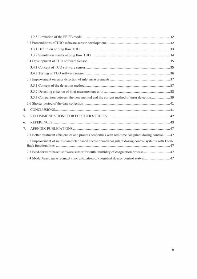
In SDWTP, the primary model for passive test was calibrated with R2=0.74 and

RMSE=53.5. The Figure 15 shows the result of passive tests over one week, comparing dosage

prediction from the CDCS and the conventional dosage. The sampling rate is 15 minutes.

SDWTP requested to obtain low TUO to reduce backwash frequency of the downstream

filtration process, therefore the expected TUO range is fixed to 0.7-1.3 NTU. At most times,

the experimental signal is able to follow the conventional signal. However, in part A the

experimental signal is much lower than the conventional signal. Since TUO is lower than the

expected range in part A, the conventional dosage as real control signal is higher than the

optimal dosage and it should be close to the experimental signal. Therefore, within a narrow

expected TUO range, the model performance is as good as the manual control by plant

operators. Similar to N2DWTP, results of the passive tests have displayed a strong basis for the

active tests.

25

Figure 15. Comparison of conventional dosing and modelled experimental dosing at the

Salcon DWTP. The thin dashed line and left axis represent the outlet turbidity, while the bold

dashed lines indicate the desired outlet turbidity range (0.7-1.3 NTU). The thin and dotted

lines refer to conventional dosage and estimated experimental dosages, respectively.

3.1.3 Results of active tests

Active tests were carried out in N2DWTP from May 2012. The CDCS was responsible

for controlling dosage in one parallel line (experimental line). Another parallel line

(conventional line) used flow-proportional dosage and the proportional ratio was decided by

plant operators. Since two lines have same inlet water quality, TUO differences between two

lines are related to dosage control. Average TUO (Avg. TUO) and standard deviation (STDEV)

are used as factors to evaluate dosage control. Table 2 shows statistical results of these two lines

(Liu et al., 2013). Over a period of one year with active tests, the model was recalibrated for

different expected TUO ranges. All monthly average TUO in the experimental line are within

the expected TUO. Some monthly average TUO in the conventional line are under the expected

TUO range, which are marked as red text. When comparing TUO stability of these two lines,

STDEV of the conventional line shows more stability in the beginning. However, STDEV of

the experimental line is lowering gradually and indicates stronger stability than the conventional

line towards the end. This could be due to the model updating with extended data. The model

with the longer training dataset leads to better performance. According to the data record in

plant SCADA, the average dosage of the experimental line is 10 % less than conventional line

during the active tests (Liu et al., 2013).

During the full-scale tests, SDWTP tested the relationship between outlet quality and

backwash frequency of subsequent filtration. Hence, expected TUO range was changed several

times. In order to deal with different expected TUO ranges, several models were calibrated.

Hence, full-scale tests in SDWTP mostly stayed in stage of passive tests under the testing

procedure.

26

Table 2, Statistical results of experimental line and conventional line in N2DWTP

Expected TUO range, NTU

Conventional line Experimental line Avg. TUO, NTU

STDEV Avg. TUO, NTU

STDEV

2012 22/4-21/5, 1st Month 1.5-2.3 1.76 0.43 1.90 0.54 2012 22/5-21/6, 2nd Month 1.5-2.3 1.35 0.51 1.88 0.72 2012 22/6-21/7, 3rd Month 1.5-2.3 1.34 0.39 1.55 0.66 2012 22/7-21/8, 4th Month 1.5-2.3 2.05 0.42 1.72 0.46 2012 22/8-21/9, 5th Month 1.5-2.3 1.85 0.30 1.53 0.36 2012 22/9-21/10, 6th Month 1.5-2.3 2.06 0.35 2.26 0.35 2012 22/10-21/11, 7th Month 1.5-2.3 1.99 0.48 2.09 0.39 2012 22/11-14/12, 8th Month 1.5-2.3 2.49 0.37 2.30 0.27 2013 15/12-14/01, 9th Month 2.3-3.0 2.38 0.43 2.50 0.26 2013 15/01-5/02, 10th Month 2.3-3.0 2.22 0.67 2.48 0.33 2013 20/02-20/03, 11th Month 2.3-3.0 2.56 0.51 2.64 0.37 2013 20/03-22/04, 12th Month 2.3-3.0 2.61 0.41 2.62 0.26

Note: STDEV: standard deviation, Avg: average.

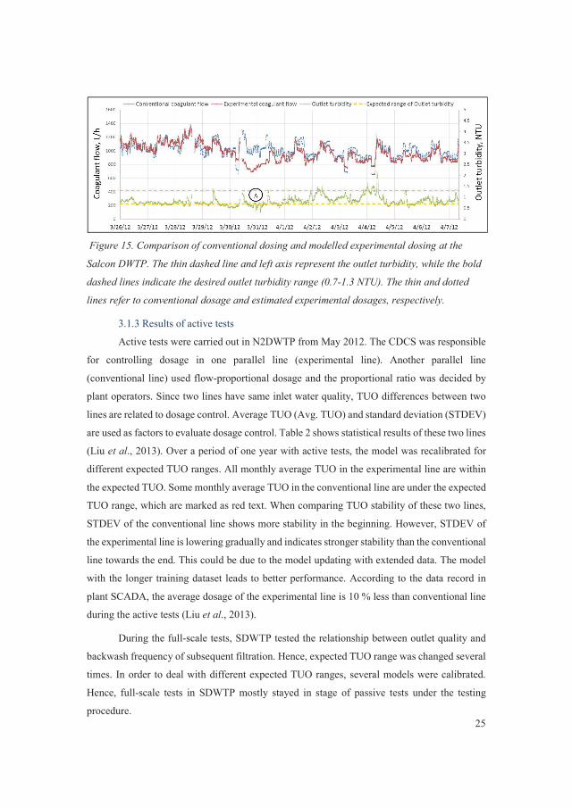
3.1.4 Dosage control during storms

It is often observed that the coagulation process experienced high TUO during storms

(Liu et al., 2013). In the Figure 16, such issues always occur in summer and dosage prediction

cannot respond to the high TUO, which are marked by “A”. Although the model was updated

with extended data that includes such a situation in 2012, the updated model still did not perform

well when storms happened again in 2013. In such situations, plant operators need to switch

control mode from the CDCS to manual control until TUO returns to the expected range. In

NRA WWTP, TUO often exceeds the requirement (less than 3 NTU) during heavy rain, as

shown in the Figure 17. In these two plants the model cannot identify such issues and adjust

dosage accordingly.

Figure 16. Large variation of outlet turbidity during storms in active tests of N2DWTP, The

situations with high TUO during storm are marked as “A”.

27

Figure 17. Large variation of outlet turbidity during wet weather in active tests of NRA

WWTP, The situations with high TUO during storm are marked as “A”.

3.1.5 Universality analysis of the CDCS

Based on the results of full-scale tests in two DWTPs, the CDCS is able to automatically

control dosage to provide acceptable and even more constant outlet quality. Simultaneously,

the CDCS displayed an ability of coagulant saving compared to manual control. Hence, the

CDCS proved to be a good solution of coagulant dosage control in DWTP. Therefore,

universality of the CDCS extended from WWTP to DWTP.

The full-scale tests showed that performance of the CDCS was unacceptable when

storms happened, which are observed not only in two DWTPs but also NRA WWTP. Such

issues indicates the limitation of model capacity of dosage control. Therefore, it is very

necessary to improve model capacity for dosage control during storms. In addition, the full-

scale tests in SDWTP displayed that the existing CDCS only focus on providing fixed outlet

quality. The expected outlet quality of the CDCS cannot change until model recalibration,

which is time-consuming. This is the reason why the full-scale tests in SDWTP mostly stayed

in stage of passive tests. Therefore, it is very necessary for the CDCS to improve the utilization

flexibility, which enables achieving different expected outlet turbidity without model

recalibration.

3.2 Improvement of model capacity

In order to improve the model capacity of dosage control and flexibility of achieving

different expected outlet turbidity, this section focuses on model improvement in view of

control strategy. The proposed solution is to add an outlet parameter into the existing FF model

to achieve feed-back control (Liu and Ratnaweera, 2016a), which is the 2nd paper of this thesis.

Firstly, measurement parameters of the CDCS are identified in view of control strategy;

28

secondly, the concept of combining FF and FB control is proposed; thirdly, the FF-FB model

is tested with operational data from N2DWTP and NRA WWTP.

3.2.1 Concept of combining feedforward and feedback model

In view of control strategy, the current model only uses the inlet quality but not outlet

quality as input variables, known as feed-forward (FF) systems or open-loop systems.

Theoretically, a FF model can react instantly to any measured disturbing variables (DVs, inlet

quality measured by online sensors) through manipulated variables (MVs, coagulant dosage)

and then controlled variables (CVs, outlet quality) will respond accordingly. In contrast, dosage

variation from a pure feed-back (FB) model only depends on outlet variables instead of inlet

variables, which means ignoring both measured and unmeasured disturbance from inlet. In

many situations, especially when the raw water source is a lake or a calm river, a FF model can

work efficiently in WWT or DWT even with a treatment process with high hydraulic delays

(Ingildsen et al., 2002). Furthermore, because a FF model is able to react at the very beginning

of a process, they lead to better economy by chemical and energy saving.

One disadvantage of the FF model is its low ability to handle situations with unmeasured

disturbance, leading to unexpected outlet quality. This is essential because there is no

compensation from outlet quality to dosage prediction. Earlier results in Chapter 3.1.4 show

that the FF model cannot respond to unexpected outlet quality during heavy rain (Liu et al.,

2013). Conversely, the advantage of the FB control is the ability to adjust dosage based on

measured error between set points and CVs. As a result, the unmeasured disturbance and related

inaccurate dosage can be compensated. Therefore, it is very necessary to incorporate the

advantages of these two control strategies with the purpose of improving model performance.

The Figure 18 shows the concept of the dosing control system combining FF with FB.

Figure 18. Control strategy of combining FF and FB

Equation 2 shows a FB as input parameter is added into the existing model, according

to the concept in Fig 18. Equation 3 shows how the FB parameter is calculated with outlet

Controller Coagulation process

Sensor

Set point Measured

error MVs CVs

DVs

+ -

Sensors

29

quality (either turbidity or suspended solid) and the set point, hence why both outlet quality and

the set point (presenting expected outlet turbidity) can influence dosage prediction.

Equation (2)

FB= ) Equation (3)

3.2.2 Validation of the FF-FB model

In N2DWTP, the FF-FB model is calibrated by dataset collected from May 2012 to

February 2013, achieving R2=0.75. Whereas the FF model (R2=0.71) is calibrated with the same

dataset, but excludes TUO. Hence, the R2 values indicate that the calibration data with TUO

provide better a fit to the FF-FB model. The Figure 19 shows the results of passive tests with

data collected from February 2013 to October 2013. The upper figure shows distributions of

TUO measurement, which includes 20 108 samples. The statistics in the lower figure shows the

dosage adjustment of the FF-FB model. The dosage adjustments are calculated with Equation

4. The results of dosage adjustments show that the FF-FB model is able to decrease the dosage

predicted by the FF model when TUO < 2.3 NTU (set point), while the adjusted dosage becomes

higher when TUO> the set point. Furthermore, the strength of this adjustment increases when

TUO becomes further away from the set point. In case of TUO > 3.8 NTU, dosage of the FF

model could not adjust adequately and the TUO starts to increase. This is because the plant

operators switched to flow-proportional dosing control and increased the dosage manually. As

a result of this, the difference between FF-FB model and real dosage is so small that dosage

adjustments show the weak strength. Otherwise, in range of 3.8-5.8 NTU, the dosage

adjustment of the FF-FB model should be approximately shown as dotted line bars. Therefore,

the FF model after adding a FB variable is able to correctly compensate the dosage prediction,

resulting in more stable TUO.

Equation (4)

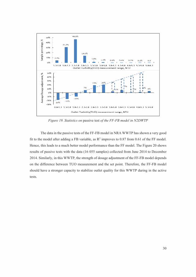
30

Figure 19. Statistics on passive test of the FF-FB model in N2DWTP

The data in the passive tests of the FF-FB model in NRA WWTP has shown a very good

fit to the model after adding a FB variable, as R2 improves to 0.87 from 0.61 of the FF model.

Hence, this leads to a much better model performance than the FF model. The Figure 20 shows

results of passive tests with the data (16 055 samples) collected from June 2014 to December

2014. Similarly, in this WWTP, the strength of dosage adjustment of the FF-FB model depends

on the difference between TUO measurement and the set point. Therefore, the FF-FB model

should have a stronger capacity to stabilize outlet quality for this WWTP during in the active

tests.

31

Figure 20. Statistics on passive test of the FF-FB model in NRA WWTP

3.2.3 Effect on coagulant consumption

Since the FF-FB model is able to adjust dosage to stabilize TUO, the coagulant

consumption will be changed accordingly. Based on statistics data in Table 4 and 5, this section

estimates potential changes of coagulant consumption under the FF-FB model control. In Table

3, the pump frequency as the system output is an indicator of coagulant flow, which is

proportional to the coagulant dosing flow. For N2DWTP, during the period of the passive tests

(9 months), the FF-FB model used 3.7 % less coagulant to prevent over-dosage. However, the

overall coagulant consumption with the FF-FB model to secure more stable TUO was 2.6 %

more than the FF model, because 12 809 data points originally had an under-dosage resulting

in TUO>2.3. Whereas in NRA WWTP the total consumption of the FF-FB model became less,

which could save 9.2 % coagulant during the passive tests (6 months). If the FB-FF model’s

task was only to reduce the over-dosage, the savings would be 15.5 %. Therefore, if inlet quality

is similar to the passive tests and TUO can work as a non-delayed FB variable, the FF-FB model

can provide approximately 9.2 % coagulant savings in future applications.

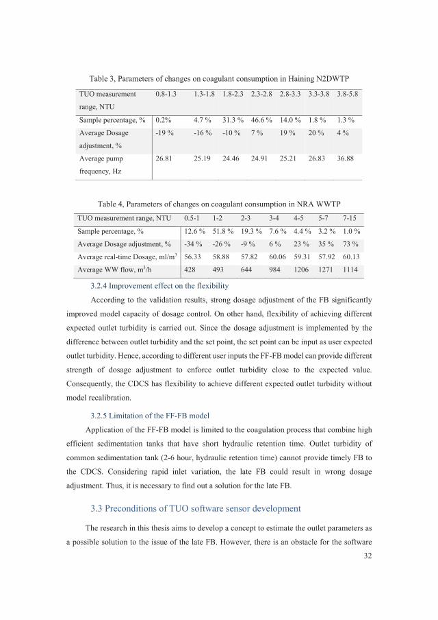
32

Table 3, Parameters of changes on coagulant consumption in Haining N2DWTP

Table 4, Parameters of changes on coagulant consumption in NRA WWTP

3.2.4 Improvement effect on the flexibility

According to the validation results, strong dosage adjustment of the FB significantly

improved model capacity of dosage control. On other hand, flexibility of achieving different

expected outlet turbidity is carried out. Since the dosage adjustment is implemented by the

difference between outlet turbidity and the set point, the set point can be input as user expected

outlet turbidity. Hence, according to different user inputs the FF-FB model can provide different

strength of dosage adjustment to enforce outlet turbidity close to the expected value.

Consequently, the CDCS has flexibility to achieve different expected outlet turbidity without

model recalibration.

3.2.5 Limitation of the FF-FB model

Application of the FF-FB model is limited to the coagulation process that combine high

efficient sedimentation tanks that have short hydraulic retention time. Outlet turbidity of

common sedimentation tank (2-6 hour, hydraulic retention time) cannot provide timely FB to

the CDCS. Considering rapid inlet variation, the late FB could result in wrong dosage

adjustment. Thus, it is necessary to find out a solution for the late FB.

3.3 Preconditions of TUO software sensor development

The research in this thesis aims to develop a concept to estimate the outlet parameters as

a possible solution to the issue of the late FB. However, there is an obstacle for the software

TUO measurement

range, NTU

0.8-1.3 1.3-1.8 1.8-2.3 2.3-2.8 2.8-3.3 3.3-3.8 3.8-5.8

Sample percentage, % 0.2% 4.7 % 31.3 % 46.6 % 14.0 % 1.8 % 1.3 %

Average Dosage

adjustment, %

-19 % -16 % -10 % 7 % 19 % 20 % 4 %

Average pump

frequency, Hz

26.81 25.19 24.46 24.91 25.21 26.83 36.88

TUO measurement range, NTU 0.5-1 1-2 2-3 3-4 4-5 5-7 7-15

Sample percentage, % 12.6 % 51.8 % 19.3 % 7.6 % 4.4 % 3.2 % 1.0 %

Average Dosage adjustment, % -34 % -26 % -9 % 6 % 23 % 35 % 73 %

Average real-time Dosage, ml/m3 56.33 58.88 57.82 60.06 59.31 57.92 60.13

Average WW flow, m3/h 428 493 644 984 1206 1271 1114

33

sensor development. In practice, water goes through the sedimentation tank by means of non-

plug flow (nonPF), which is not as ideal as plug-flow (PF). Hence, potential mixing effect could

exist under the nonPF. Consequently, TUO measurements present the mixing results of

different PF TUOs. Therefore, it is necessary to confirm if TUO measurements are accurate

results of inlet quality and dosage. In order to test the mixing effect, this section simulates PF

TUO and compares with TUO measurement (Liu and Ratnaweera, 2016b), as the 3rd paper of

this thesis. This section is a precondition of the software sensor development, which is

illustrated in the next chapter.

3.3.1 Definition of plug flow TUO

Definition of PF TUO in this thesis is based on tracer tests. Results of tracer tests were

previously carried out in NRA WWTP (Rathnaweera, 2010). After a certain dosage of tracer

(Rhodamin B) was added at inlet of sedimentation, results show that the tracer concentration at

outlet of the sedimentation tank distributes with time. Thus, PF TUO can be defined by the

distribution ratio and TUO measurement. This concentration distribution illustrates that each

water segment at time t0 tends to distribute a certain amount of itself to other nearby water

segments at times t±n, which is the process of converting PF TUO to nonPF TUO. Hence, PF

TUO at time t0 equals many distributions that provide to TUO measurements at time t0 and

t±n. Furthermore, the distribution of tracer concentration indicates the distribution range and

ratio of PF TUO. According to the concept, Equation 5 illustrates the definition of PF TUO,

where percentages present the distribution ratio and t±n indicates the distribution range.

In order to find out the significance of the distribution effect, PF TUO is simulated by

Equation 5 under different distribution ratio of water segments, which is shown in Table 5.

Considering the tracer test results, the longest mixing range in this paper is assumed as -90

minutes to +30 minutes. Since the water segments are measured every 15 minutes, the nine

segments are considered to represent the distribution ratio as noted in Table 5

PF TUOt0 = (TUOt-6*a % + TUOt-5*b % + TUOt-4*c % + TUOt-3*d % + TUOt-2*e % +

TUOt-1*c % + TUOt0*d % + TUOt+1*e % + TUOt+2*f %) Equation (5)

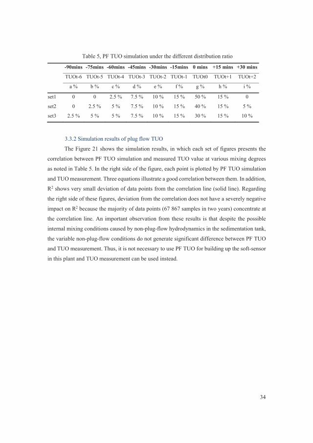
34

Table 5, PF TUO simulation under the different distribution ratio

-90mins -75mins -60mins -45mins -30mins -15mins 0 mins +15 mins +30 mins

TUOt-6 TUOt-5 TUOt-4 TUOt-3 TUOt-2 TUOt-1 TUOt0 TUOt+1 TUOt+2

a % b % c % d % e % f % g % h % i %

set1 0 0 2.5 % 7.5 % 10 % 15 % 50 % 15 % 0

set2 0 2.5 % 5 % 7.5 % 10 % 15 % 40 % 15 % 5 %

set3 2.5 % 5 % 5 % 7.5 % 10 % 15 % 30 % 15 % 10 %

3.3.2 Simulation results of plug flow TUO

The Figure 21 shows the simulation results, in which each set of figures presents the

correlation between PF TUO simulation and measured TUO value at various mixing degrees

as noted in Table 5. In the right side of the figure, each point is plotted by PF TUO simulation

and TUO measurement. Three equations illustrate a good correlation between them. In addition,

R2 shows very small deviation of data points from the correlation line (solid line). Regarding

the right side of these figures, deviation from the correlation does not have a severely negative

impact on R2 because the majority of data points (67 867 samples in two years) concentrate at

the correlation line. An important observation from these results is that despite the possible

internal mixing conditions caused by non-plug-flow hydrodynamics in the sedimentation tank,

the variable non-plug-flow conditions do not generate significant difference between PF TUO

and TUO measurement. Thus, it is not necessary to use PF TUO for building up the soft-sensor

in this plant and TUO measurement can be used instead.

35

Figure 21. Significance of mixing effect under different mixing percentage

3.4 Development of TUO software Sensor

Based on the above conclusion that the non-plug-flow conditions have insignificantly

impacted the composition of the outlet water portions, this section presents development of the

TUO software-sensor using shifted TUO measurement (Liu and Ratnaweera, 2016b).

3.4.1 Concept of TUO software sensor

In Figure 22, the proposed TUO software-sensor, encircled by the dotted line, lies in

front of the sedimentation tank, which can predict TUO measurement. According to simulation

results of PF TUO in Chapter 3.3.2, PF TUO can be generally represented by TUO

measurements (nonPF TUO) with small errors. Hence, the model of the TUO software-sensor

can be built up with existing inlet water parameters, dosage and TUO measurements instead of

PF TUO. Equation 6 shows the model structure of the software-senor. PLSR and Unscrambler®

(version 10.3) are used for building up the relationship between inlet parameters, dosage and

TUO measurement. Regarding dataset preparation, TUO measurements are shifted and

matched to inlet parameters considering the theoretical HRT.

36

Equation (6)

Figure 22. Concept of the TUO software-sensor (Instruments covered solid line present

physical online sensors whereas the TUO software-sensor within the dotted line)

3.4.2 Testing of TUO software sensor

A model of the TUO software-sensor was calibrated with the dataset collected in 2013.

R2=0.86, as coefficient determination of calibration, indicates that the dataset fits the model.

The Figure 23 shows the results of model validation with the dataset collected in 2014. X-axis

stands for TUO prediction with inlet parameter, while Y-axis shows the corresponding TUO

measurement (shifted TUO). Regarding the regression line, the slope (1.025) and intercept

(0.186, crossing point with Y-axis) shows that the correlation line is very close to an ideal line

Y=X, and R2 indicates that most data points centralize to the correlation line.

Figure 23. Correlation between shifted TUO and TUO prediction. The dotted line shows the

ideal fit.

37

According to the results of accuracy analysis (Liu et al., 2016b), accuracy of TUO

prediction is 84 % in the majority range 1-5 NTU. Even with somewhat higher relative errors,

the error in absolute values are less than 0.31 NTU for the working range (1-5 NTU), which is

promising.

In full-scale treatment, it is often not an objective to obtain the lowest possible TUO,

but an adequately good TUO. In most cases, TUO within 1-5 NTU is considered as an

acceptable optimal. Sensitivity of model performance, which depends on the majority of the

dataset, is not good enough when predicting TUO at low levels. Thus, the expected range of

TUO measurement is mostly overlapped with the optimal working range of TUO software-

sensor (1-5 NTU). When the TUO software-sensor is used as a FB for dosage control, the

adjusted dosage will cause a narrower range of TUO measurement, where the software-sensor

has a better performance.

3.5 Improvement on error detection of inlet measurements

Performance of the coagulant dosage control system highly depends on working status

of online sensors. Although routine maintenances (cleaning and calibration) are carried out

regularly by plant operators, measurement errors usually occur and challenge the reliability of

the dosage control system. Thus, measurement error detection is an essential part of the dosage

control system. Relying on the software sensor, this section is to build up a new method to

detect inlet measurement errors (Liu et al., 2016c), which is the 4th paper of this thesis.

3.5.1 Concept of the detection method

TUO measurements can be used as a reference in error detection of inlet measurements.

As an indicator of treatment results, TUO measurements can respond to any change of related

inlet parameters and dosage. Either under-dosage or over-dosage can cause TUO measurement

outside of the expected range. Thus, TUO is a key parameter for the coagulation process. In

practice, not only are turbidity sensors (or suspended solid sensors) sometimes double or triple

installed at a process outlet, the TUO laboratory measurements are often used to compare with

online TUO measurements to ensure its accuracy. Moreover, an improved working

environment at the process outlet, where most particles settle down, reduces the error

proneness of the TUO sensors. Therefore, TUO sensors are the most reliable instruments in

the dosage control system and are able to function as the reference in the error detection.

38

The software sensor, presented in Chapter 3.4, enables the simulation of TUO at given

inlet parameters and dosage. Hence, differences between TUO measurements and

corresponding TUO simulations are generated. This thesis considers that these differences are

caused by both model errors and inlet measurement errors. Model errors exist in all TUO

simulations with unpredictable fluctuations around the mean value. This thesis assumes that

model errors repeat within a certain range and the related differences are limited to the certain

range accordingly. However, the differences caused by inlet measurement errors are similar to

systematic errors, which happen occasionally with definite causes such as sensor faults, wrong

calibration, communication pause, etc. Thus, the proposed concept of the error detection is that

when the differences exceed the certain range that the model errors decide, the measurement

errors of inlet sensors are considered to be the cause. The Figure 24 describes the above

concept, where the red lines indicate that inlet measurement and model are sources of

difference.

Figure 24. Concept of error detection of inlet measurements, the red lines indicate

sources of difference

3.5.2 Detecting criterion of inlet measurement errors

Since there is an obvious boundary between model errors and inlet measurement errors,

this section defines a criterion of error detection based on the boundary (Liu et al., 2016c). The

Figure 25 shows the correlation between TUO measurement (Y-axis) and TUO simulation (X-

axis). Liu et al. (2016) proved that the model of TUO prediction is constant after several

recalibrations with different random selection samples, so that the slope and offset are constant

accordingly. Two lines (dotted lines) parallel with the correlation line are added to indicate the

boundary between model errors and inlet measurement errors. These two lines are expressed

by the Equation 7. Hence, these two lines can function as the detection criterion of inlet

measurement errors. Namely, if a plotted point (a TUO measurement, a TUO simulation) lies

between two lines described by Equation 8, there is an insignificant difference between TUO

Inlet Measurements Model

TUO Simulation

Difference Inlet measurement errors, if the difference is outside the certain range

NO inlet measurement error, if the difference is within the certain range.

Dosage

39

simulation and TUO measurement, hence inlet online sensors are working normally. Otherwise,

plotted points lying outside these two lines indicate measurement errors of inlet online sensors.

Equation 7

Equation 8

Figure 25. Detection criterion of inlet measurement errors, Solid line presents

correlation line between simulations (X-Axis) and measurements (Y-Axis) of outlet turbidity.

Based on the slope and the offset of the correlation line and defined range of model errors,

two dotted lines parallel with the correlation line are defined as proposed detection criterion.

Offset of additional lines=offset of correlation line ± K)

3.5.3 Comparison between the new method and the current method of error detection

In the previous section, the new detection method of inlet measurement errors was

developed based on the software sensor. In order to prove the better efficiency of the newly

developed method over the current method, the following section compares these two methods

(Liu et al., 2016c).

Two detection criterions (normal measurement range and variation validation) as the

current method are responsible for detecting inlet measurement errors. The outliers detected by

the normal variation range are assumed to influence TUO simulation and to generate significant

differences between TUO simulation and TUO measurement. All points in the Figure 26 are

checked with two current detection criterions and any point related to measurement errors are

marked. The plotted points marked with various shapes represent different erroneous

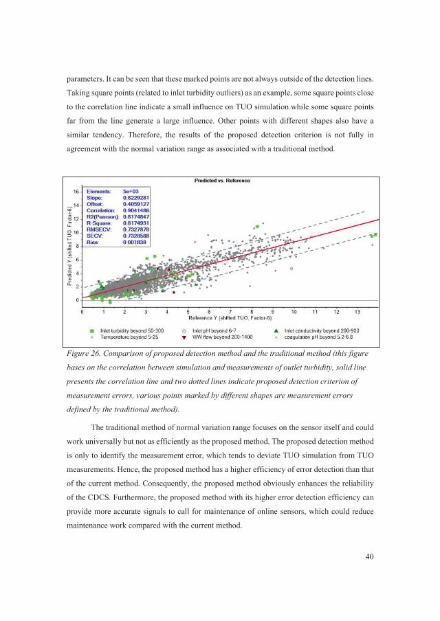
40

parameters. It can be seen that these marked points are not always outside of the detection lines.

Taking square points (related to inlet turbidity outliers) as an example, some square points close

to the correlation line indicate a small influence on TUO simulation while some square points

far from the line generate a large influence. Other points with different shapes also have a

similar tendency. Therefore, the results of the proposed detection criterion is not fully in

agreement with the normal variation range as associated with a traditional method.

Figure 26. Comparison of proposed detection method and the traditional method (this figure

bases on the correlation between simulation and measurements of outlet turbidity, solid line

presents the correlation line and two dotted lines indicate proposed detection criterion of

measurement errors, various points marked by different shapes are measurement errors

defined by the traditional method).

The traditional method of normal variation range focuses on the sensor itself and could

work universally but not as efficiently as the proposed method. The proposed detection method

is only to identify the measurement error, which tends to deviate TUO simulation from TUO

measurements. Hence, the proposed method has a higher efficiency of error detection than that

of the current method. Consequently, the proposed method obviously enhances the reliability

of the CDCS. Furthermore, the proposed method with its higher error detection efficiency can

provide more accurate signals to call for maintenance of online sensors, which could reduce

maintenance work compared with the current method.

41

3.6 Shorter period of data collection

According to the procedure of the CDCS implementation, data collection is the

essential step after the installation of online sensors and the CDCS. Previously, it was very

necessary to collect as much data as possible to obtain influent information, improve the

empirical model’s performance. Normally, this step needed a long time until the model

performance proved to be acceptable. Hence, it is a time-consuming method to undertake prior

to real dosage control. As an enhanced feature of the CDCS, this disadvantage can be

compensated by the FF-FB model. The effect of the FB control shows a strong ability to adjust

the inaccurate dosage that is calculated from the FF model. Thus, with the CDCS it is possible

to shorten the data collection period (calibration period) and start the active dosing control

earlier than before.

4. CONCLUSIONS

• The dosage control system was improved and verified in two DWTPs. Consistently

improved treated water qualities and operational economies, also under extreme

conditions, were documented in comparison to manual dosage control. The extended

tests from WWTPs to DWTPs expanded the application universality of the dosing

control system.

• The feedforward-feedback (FF-FB) model is built up by involving an outlet parameter

as feedback. The feedforward-feedback (FF-FB) model proved more able to provide

stronger capacities on dosage control than the previous feedforward (FF) model.

Moreover, the feedforward-feedback (FF-FB) model is able to provide further coagulant

savings compared to the previous feedforward model.

• The feedforward-feedback model with user input can achieve different outlet targets

that considerably improves utilization flexibility of the coagulant dosage control system.

• Non-plug-flow condition of the sedimentation tank assumes to mix treated water

batches, which is a potential obstacle for establishing a quantitative relationship

between treated water quality and inlet parameters. This thesis proposes a method for

simulating mixing effect and outlet turbidity under the plug-flow condition. It proved to

42

be a useful solution to confirm whether the mixing condition has a significant effect on

the outlet turbidity.

• The hydraulic retention time resulting from the conventional sedimentation tanks

hinders the application of the feedforward-feedback model. This thesis proposes a soft-

sensor for outlet turbidity. The software sensor can predict outlet turbidity before it is

measured. Hence, it can highly contribute the feedforward-feedback model to have wide

applications in the coagulation processes that involve conventional sedimentation tanks.

• Based on the outlet turbidity estimated by the software sensor, the novel method of inlet

measurement error detection was developed to have a higher efficiency of error

detection than previous methods. The novel method improved the reliability of the

dosage control system.

• The dosage control system is enhanced by several solutions that underpin the thesis

focus. An enhanced system with these solutions can enable a shorter period of data

collection and improved operational economy.

5. RECOMMENDATIONS FOR FURTHER STUDIES

• Implementing further full-scale tests with the enhanced CDCS, especially in DWTP

during storms.

• Involving more parameters as model inputs like phosphates, colour, hardness, etc.

• Developing other software sensors to predict different outlet parameters such as

phosphate, colour, remaining aluminium, etc.

• With a broad operational data base, further attempts should be made to develop

conceptual models.

43

6. REFERENCES

Adgar A., Cox C.S. & Jones C.A. 2005, ‘Enhancement of coagulation control using the streaming current detector’, Bioprocess Biosyst, vol. 27, pp. 349–357.

AlGhazzawi A. & Lennox B. 2009, ‘Model predictive control monitoring using multivariate statistics’, Journal of Process Control, vol.19, no.2, pp. 314-327.

Amari S., Murata N., Müller K.R., Finke M. & Yang H.H., 1997, ‘Asymptotic statistical theory of overtraining and cross-validation’, IEEE Transactions on Neural Networks, vol. 8, no. 5, pp. 985–996.

Amirtharajah A. & Mills K.M. 1982, ‘Rapid Mix Design for Mechanisms of Alum Coagulation’, Jour. AWWA, vol. 74, pp. 4-210.

American Water Works Association (AWWA). ‘Operational Control of Coagulation and Filtration Processes, in Manual of Water Supply Practices’, 3rd ed., AWWA: Denver, USA, 2011

Baxter C.W., Stanley S.J. & Zhang Q. 1999, ‘Development of a full-scale artificial neural network model for the removal of natural organic matter by enhanced coagulation’, Journal of Water SRT-Aqua, vol. 48, no. 4, pp. 129–136.

Baxter C.W., Zhang Q., Stanley S.J., Shariff R., Tupas R.T. & Stark H.L. 2001, ‘Drinking water quality and treatment: the use of artificial neural networks’, Canadian Journal of Civil Engineering, vol. 28, pp. 26–35.

Baxter C.W., Shariff R., Stanley S.J., Smith D.W., Zhang Q. & Saumer E.D. 2002, ‘Model based advanced process control of coagulation’, Water Science and Technology, vol. 45, no. 4-5, pp. 9-17.

Beckhoff, 2015, ‘New Automation Technology’, https://www.beckhoff.com/, (accessed 26 December 2015).

Bloch G. & Denoeux T. 2003, ‘Neural networks for process control and optimization: Two industrial applications’, ISA Trans, vol. 42, pp. 39–51.

Camo, 20015, ‘Bring data to life’, http://www.camo.com/, (accessed 22 December 2015). Dayal B.S. & MacGregor J.F. 1997, ‘Improved PLS algorithms’, J. Chemometrics, vol. 11,

no.1, pp. 73-85. De Jong S. & Ter Braak C. J. F. 1994, ‘Comments on the PLS kernel algorithm’ J.

Chemometrics, vol. 8, pp. 169-174. Dellana S.A. & West D. 2009, ‘Predictive modelling for wastewater application: Linear and

nonlinear approaches’, Environmental Modelling & Software, vol. 24, pp. 96-106 Dentel S.K. & Kingery K.M. 1898, ‘Theoretical principal of streaming current detection’,

Water Science and Technology, vol. 21, pp.443-453. Dentel S.K. 1991, ‘Coagulant control in water treatment’, Critical reviews in environmental

control, vol. 21, no.1, pp. 71-75. Dentel S.K. & Abu-Orf MM. 1995, ‘Laboratory and full-scale studies of liquid stream

viscosity and streaming current for characterization and monitoring of dewaterability’, Water Research, vol. 29, no.12, pp. 2663-2672.

Fortuna L., Graziani S., Rizzo A. & Xibilia M. ‘Soft Sensors for Monitoring and control of Industrial Process’, Springer Science, London, 2007.

Guida M., Mattei M., Della Rocca C., Melluso G. & Meric S. 2007, ‘Optimization of alum-coagulation/flocculation for COD and TSS removal from five municipal wastewater’, Desalination, vol. 211, pp. 113–127.

Guo Y.F., Ma J., Zhai X.D. & Fan Y. 2009, ‘Flocculent Dosage Optimizing in Water Treatment based on Nonlinear Mathematical Model’, International Conference on Environmental Science and Information Application Technology

44

Hamed M.M., Khalafallah M.G. & Hassanien E.A. 2004, ‘Prediction of wastewater treatment plant performance using artificial neural networks’, Environmental Modelling & Software, vol. 19, no. 10, pp. 919-928.

Hangouet J.P., Pujol R., Bourgogne P., Ropert D. & Lansalot G. 2007, ‘Optimizing chemical dosage in primary settling tanks’, Chemical Water and Wastewater Treatment IX, Proceeding of the 12th Gothenburg Symposium 2007, Hermann H. Hahn Erhard Hoffmann Hallvard Ødegaard (eds), IWA Publishing, London, pp.59-67.

Huang M.Z., Ma Y.W., Wan J.Q. & Wang Y. 2009, ‘Simulation of a paper mill wastewater treatment using a fuzzy neural network’, Expert Systems with Applications, vol. 36, no. 3, pp. 5064-5070.

Hunter R.J. ‘Zeta Potential in Colloids Science’, Academic Press, New York, 1981. Hunter R.J. ‘Foundations of Colloid Science’, Oxford University Press Inc., New York, 2001. Ingildsen P., Jeppsson U. & Olsson G. 2002, ‘Dissovled oxygen controller based on on-line

measurements of ammonium combinning feed-forward and feedback’, Water Science and Technology, vol. 45, no. 4-5, pp.453-460.

Jeppsson U., Alex J., Pons M.N., Spanjers H. & Vanrolleghem P.A. 2002, ‘Status and future treads of ICA in wastewater treatment-A European perspective’, Wat. Sci. Tech, vol. 45, no. 4-5, pp. 485-494.

Joo D.S., Choi D.J. & Park H.Y. 2000, ‘The effects of data preprocessing in the determination of coagulation dosing rate’, Wat. Res. vol. 34, no. 13, pp. 3295-3302.

Kan C.C. & Huang C. 1998, ‘Coagulation monitoring in surface water treatment facilities’, Water Science and Technology, vol. 38, no. 3, pp. 237–244.

Li J.G., Dhanvantari S., Averill D. & Biswas N. 2003, ‘Windsor combined sewer overflow treatability study with chemical coagulation’, Water Qual. Res. vol. 38, no. 2, pp. 317-334.

Lu L. 2003, ‘Model based control and simulation of wastewater coagulation’, PhD thesis, Agriculture University of Norway

Liu W., Ratnaweera H. & Song H.P. 2013, ‘Better treatment efficiencies and process economies with real-time coagulant dosing control’, 11th IWA conference on instrumentation control and automation, France

Liu W., & Ratnaweera H. 2016a, ‘Improvement of multi-parameter based Feed-Forward coagulant dosing control systems with Feed-Back functionalities’, Water Science and Technology (accepted)

Liu W., & Ratnaweera H. 2016b, ‘Feed-forward based software sensor for outlet turbidity of coagulation process’, Journal Sensors (submitted)

Liu W., Ratnaweera H. & Knut K, 2016, ‘Model based measurement error estimation of coagulant dosage control system’, Journal Water (submitted)

Lindgren F., Geladi P. & Wold S. 1993, ‘the kernel algorithm for PLS’, J. Chemometrics, vol. 7, no.1, pp. 45-59.

Maier H.R., Morgan N. & Chow W.K. 2004, ‘Use of artificial neural networks for predicting optimal alum doses and treated water quality parameters’, Environmental Modelling & software, vol. 19, no. 5, pp. 485-494.

Maier, H.R., Jain A., Dandy G.C. & Sudheer K.P. 2010, ‘Methods used for the development of neural networks for the prediction of water resource variables in river system: Current status and future directions’, Environmental Modelling & Software, vol. 25, pp. 891-909.

Manamperuma L., Ratnaweera H., Heistad A., Martsul A. & Vasenko L. 2015, ‘Impact on plant availability of phosphorus in sludge after coagulation’, Conference on Nutrient IWA, Removal and Recovery: moving innovation into practice 2015, Gdansk, Poland.

Oh J.I. & Lee S.H. 2005, ‘Influence of streaming potential on flux decline of microfiltration with in-line rapid pre-coagulation process for drinking water production’, J. Membr. Sci. vol. 254, pp. 39–47.

45

Rathnaweera S. 2010, ‘Modelling and Optimization of Wastewater Coagulation Process’, PhD thesis, Norwegian University of Life Sciences.

Ratnaweera H. 1991, ‘Influence of the degree of coagulant preploymerization on wastewater coagulation mechanisms’, Doctoral thesis, Norwegian Institute of Technology, Dissertation publishing, Michigan, USA.

Ratnaweera H., Blom H. & Aasgaard G., 1994, ‘Flexible coagulant dosing control system based on real-time wastewater quality monitoring’, Chemical water and wastewater treatment III, Hahn, H.H and Klute, R (eds), Springer-Verlag, Berlin, pp. 105-116.

Ratnaweera H., Lu L. & Lindholm O. 2002, ‘Simulation Program for Wastewater Coagulation, Chemical Water and Wastewater Treatment vii’, H.H.Hahn, E.Hoffmann and H. Oedegaard (eds), Gothenburg, Sweden, IWA publishing, London, pp. 253-260.

Ratnaweera H., Lei L., & Lindholm O. 2002, ‘Simulation program for wastewater coagulation’, Water Science and Technology, vol. 46, no. 5, pp. 27-33.

Ratnaweera H. 2004, ‘Coagulant dosing control-a review’, Chemical water and wastewater treatment VIII, HH Hahn, E Hoffmann, H Ødegaard (eds), IWA Publishing, London, pp. 3-13.

Ratnaweera H., Smoczy ski L., Lewandowski A. & Bielecka M. 2005, ‘Efficient Coagulant Dosing Control in Wastewater Treatment’, Pol. Acad. Sci. vol. 505, pp. 347–352.

Ratnaweera H. & Fettig J. 2015, ‘State of the Art of Online Monitoring and Control of the Coagulation Process’, Water, vol. 7, pp. 6574-6597.

Rietveld L. & Dudley J. 2006, ‘Models for Drinking water treatment-review state of the art’, Report TECHNEAU, European Commission under the Sixth Framework Programme.

Sharp E. & Norris R. 2015, ‘Using online zeta potential measurements for coagulation control: A first for the UK water industry’. In Proceedings of the 6th IWA Specialist Conference on Natural Organic Matter in Drinking Water, Malmö, Sweden.

Shutova Y., Baker A., Bridgeman J. & Henderson R.K. 2014, ‘Spectroscopic characterization of dissolved organic matter changes in drinking water treatment: From PARAFAC analysis to online monitoring wavelengths’, Water Res. vol. 54, pp. 159–169.

Scherrenberg S.M. 2006, ‘Treatment Techniques for Combined Sewer Overflows: A literature study of the available techniques’, Master Thesis, Delft University of Technology.

Schlenger D.L., Riddle W.F., Luck B.K. & Winter, M.H. 1996, ‘Automation Management Strategies for Water Treatment Facilities’, Denver, CO.: AWWARF and AWWA.

Siriprapha J., Sinchai K. & Suwapee T. 2011, ‘Evaluation of reusing alum sludge for the coagulation of industrial wastewater containing mixed anionic surfactants’, Journal of Environmental Sciences, vol. 23 no. 4, pp. 587-594.

Stumm W. & O’melia C.R. 1968, ‘Stoichiometry of Coagulation’ Jour. AWWA, vol. 60, no. 5, pp. 514-539.

Stumm W. & Morgan J. 1995, ‘Aquatic Chemistry: Chemical Equilibria and Rates in Natural Water’, John Wiley & Sons, Inc. New York.

Stanley SJ., Baxter CW. & Zhang Q. ‘Process Modelling and Control of Enhanced Coagulation’, AWWA research Foundation’, USA, 2000.

Svante W., Michael S. & Lennart E. 2001, ‘PLS-regression: a basic tool of Chemometrics’, Chemometrics and Intelligent Laboratory Systems, vol. 58, pp. 109–130.

Tchobanoglous G., Burton F. & Stensel D. 1997, ‘Water Engineering: Treatment and Reuse’, Edition 4, McGraw-Hill, Inc, New York.

Vanrolleghem P.A. & Lee D.S. 2003, ‘On-line monitoring equipment for wastewater treatment process, State of the art’, Water Science and Technology, IWA publishing, vol. 47 no.2, pp. 1.

Walker C.A., Kirby J.T. & Dentel S.T. 1996, ‘the Streaming Current Detector: A Quantitative Model’, Journal of Colloid and Interface Science, vol. 182, no. 1, pp. 71-81.

46

Wu G.D. & Lo S.L. 2008, ‘Predicting real-time coagulant dosage in water treatment by artificial neural networks and adaptive network-based fuzzy inference system’, Engineering Applications of Artificial Intelligence, vol. 21, no. 8, pp. 1189-1195.

Wu G.D. & Lo S.L. 2010, ‘Effects of data normalization and inherent-factor on decision of optimal coagulant dosage in water treatment by artificial neural network’, Expert Systems with Applications, vol. 37, no.7, pp. 4974-4983.

Yu R.F., Kang S.F., Liaw S.L. & Chen M. 2000, ‘Application of artificial neural network to control the coagulant dosing in water treatment plant’, Water Science and Technology, vol. 42, no. 3-4, pp. 403-408.

Yu W.Z., Gregory J., Campos L. & Li G. 2011, ‘The role of mixing conditions on floc growth, breakage and regrowth’, Chemical Engineering Journal, vol. 107, pp. 425-430.

Zeng G.M., Qin X.S., He L., Huang G.H., Liu H.L. & Lin Y.P. 2003, ‘A neural network predictive control system for paper mill wastewater treatment’, Engineering Applications of Artificial Intelligence, vol. 16, no. 2, pp. 288-291.

Zhang Q. & Stanley S. 1999, ‘Real-Time Water Treatment Process Control with Artificial Neural Networks’, J. Environ. Eng., vol. 125, no. 153, pp. 153-160.

47

7. APENDIX-PUBLICATIONS

7.1 Better treatment efficiencies and process economics with real-time coagulant

dosing control

Wei Liu, Harsha Ratnaweera, Heping Song

Paper presented at 11th IWA Conference on Instrumentation Control and Automation

(ICA2013), Narbonne, France, 2013

7.2 Improvement of multi-parameter based Feed-Forward coagulant dosing control

systems with Feed-Back functionalities

Wei Liu, Harsha Ratnaweera

Paper accepted by Journal Water Science and Technology

7.3 Feed-forward based software sensor for outlet turbidity of coagulation process

Wei Liu, Harsha Ratnaweera

Paper is submitted to International Journal of Research & Development

Organization

7.4 Model based measurement error estimation of coagulant dosage control system

Wei Liu, Harsha Ratnaweera and Knut Kvaal

Paper is submitted to International Journal of Environmental Science and Technology

Paper I

Better treatment efficiencies and process economics with

real-time coagulant dosing control

Wei Liu, Harsha Ratnaweera, Heping Song

Paper presented at 11th IWA Conference on Instrumentation Control and

Automation, Narbonne, France, 2013

Better treatment efficiencies and process economics with real-

time coagulant dosing control

L Wei*, H. Ratnaweera*, S. Heping**

*Norwegian University of Life Sciences, PO Box 5003-IMT, 1432 Aas, Norway. Email: wei.liu@umb.no

** Jiaxing ROSIM Co LtD, No1369 Chengnan Road, Jiaxing 314001, P.R. China.

ABSTRACT

Coagulation is the most widespread method for treatment of drinking water in the

world. Accurate dosing of coagulants is vital both for health and process economics. Inability

to estimate accurate dosages may result in poor treatment, high coagulant costs and negative

subsequent in downstream processes. The optimal dosage depends on not only flow and pH

but also particles, color and other impurities in raw water. By including these parameters in

the estimation of optimal dosage, one can achieve significant process and economic

improvements. A dosing control concept originally developed for wastewater treatment was

modified and tested at full-scale with very good results. The treatment efficiencies were not

only better but also proved possible to manage within desired outlet ranges, thus enabling a

dosing control tailored for desired outlet turbidities. A comparison of performances between

a flow proportional and multi-parameter based dosing control system is given with cost

savings, while securing improved outlet qualities.

Keywords: coagulation; dosing control; drinking water treatment

1. INTRODUCTION

Coagulation is the world’s most commonly used treatment method in drinking water

treatment. Aluminum is the most common coagulant but it has two major disadvantages:

Firstly, coagulation with aluminum functions within a narrow pH range, thus an optimal

dosage is required to obtain the best performance as well as to achieve less coagulant cost

(Gregory et al., 1997). Secondly, an overdosing of aluminum or dosing under a wrong pH

range might result in dissolved aluminum species in the treated water rather than the species

that are favorable for coagulation (Rebhun and Lurie, 1993). Since the aluminum in drinking

water is identified to be a potential risk factor for Alzheimer disease (Guidelines for drinking

water quality, 2008), non-optimal dosage may create a health risk.

Since conditions of the plant operation and coagulant are more or less constant for a

given plant, the optimal coagulant dosage is mainly dependent on parameters of water quality

that include the content of particles, color produced by Natural Organic Matter (NOM) and

coagulation pH (Edzwald J.K., 1993). However, most drinking water treatment plants

(DWTP) in the world use a flow proportional dosage, sometimes combined with pH (Dentel,

1991). Some smaller DWTPs even use constant, time proportional dosage. Although it won’t

be a problem for DWTPs using raw water from lakes with rather stable water qualities,

DWTPs using polluted and turbulent rivers as water source often experience rapid changes in

raw water quality, which challenges the estimation of optimal dosage. Because the importance

of these critical parameters is ignored, such practices often cause poor treatment results, high

coagulant dosage and high operational costs. Moreover, the high coagulant dosage may also

increase the filter load of downstream processes, which could results in process complications

and higher operational costs.

The general understanding of the coagulation process indicates that the optimal dosage

depends on water quality parameters like particles and colour, in addition to the commonly

used flow and pH. However, it has been a challenge to achieve better dosing control systems

due to the additional cost of online water quality instruments and the lack of suitable

algorithms. Although the online instruments are now much more accessible and affordable

than they were few years ago, suitable algorithms integrated with several parameters are still

scarce (Ratnaweera, 2004).

DOSCON has developed a concept using multi-parameter surveillance of water

quality for determination of the optimal coagulant dosage in real-time. Inputs used for dosage

prediction in the DOSCON system include inlet flow, turbidity, conductivity, temperature,

pH, and coagulation pH. The concept was initially developed for wastewater treatment

(Ratnaweera et al, 2005) and further improved later (Rathnaweera, 2010). This paper presents

its extension to drinking water treatment, which is verified by the full-scale tests.

The DWTPs, where the full-scale tests were conducted, had requirements of outlet

turbidity within the limit (less than 3 NTU) in coagulation process considering the conditions

for optimal performance of downstream treatment process. Until the experimental system was

installed, operators daily adjusted the coagulant dosage manually by judging the outlet quality

in the full-scale plant. Since the water quality varied regularly, it was a demanding task to

keep turbidity within the requested range, especially during the rainy seasons. This paper

presents the verification results of application of a multi-parameter based coagulant dosing

control system for DWTPs.

2. MATERIALS AND METHODS

The full-scale tests were conducted at two DWTPs near Shanghai, Haining DWTP2

(capacity: 100 000m3/day) and Salcon DWTP (capacity: 300 000 m3/day). Both DWTPs

receive water from the Changshan River where the water quality can vary significantly during

a rainy period or a typhoon. The existing dosing strategy of both plants was flow proportional

dosing.

Both DWTPs had some online instrumentation and were supplemented with others so

the turbidity, pH, conductivity, temperature and flow in the inlet and pH and turbidity in the

outlet were possible to monitor online. These signals were acquired in real-time by the

Supervisory Control and Data Acquisition (SCADA) system of the DWTPs that were then

processed by the DOSCON unit, consisting of an embedded PC and a range of algorithms.

Both plants have parallel treatment lines with the same water quality, hence it was possible to

carry out the experiment with one treatment line using the conventional (flow proportional)

dosing while a separate treatment line used the experimental (multi-parameter) dosing control

system. The system started to collect operational data, which was used as calibration sets, as

the generic algorithms of the DOSCON system need to be calibrated for each DWTP. After a

special selection process of suitable datasets, the data were analyzed and relevant models

constructed using software Unscrambler®.

3. RESULTS AND DISCUSSION

The ambition of the DWTPs was to keep the outlet turbidity just below 3 NTU. In

practice, the outlet turbidity was well below the anticipated values, because the plants were

unable to adjust dosage to result in exactly below 3 NTU with the conventional dosing control

system. The result was to use a slightly higher dosage than the optimal dosage to secure

effluent turbidities below required levels, which gave much lover effluent values at times.

Figure 3.1. Comparison of conventional dosing and modelled experimental dosing

at the Haining DWTP No 2. The thin dashed line and left axis represent the outlet turbidity,

while the bold dahsed lines indicate the desired outlet turbidity range (2.0-3.0 NTU). The

thin and dotted lines refer to conventional dosage and estimated experimental dosages,

respectively.

Figure 3.2. Comparison of conventional dosing and modelled experimental dosing at

the Salcon DWTP. The thin dashed line and left axis represent the outlet turbidity, while the

bold dashed lines indicate the desired outlet turbidity range (0.7-1.3 NTU). The thin and

dotted lines refer to conventional dosage and estimated experimental dosages, respectively.

Fig 3.1 and Fig 3.2 present the results under the traditional flow proportional dosing

control over a 10-day period in 2012, together with modelled dosing values using the

experimental concept. As it is seen from the figures, the outlet turbidity (thin dashed line),

on several occasions has gone beyond the desired range (bold dashed lines). A closer look at

the data reveals that those periods when the outlet turbidity is beyond the maximum values

the experimental dosage proposes a higher dosage than the conventional dosage. It also

shows the opposite when the outlet turbidity is too low, which confirms the superiority of

the experimental dosing concept.

Figure 3.3. Comparative results from the experiments at the Haining DWTP No 2.

The thin dashed line and left axis represent the outlet turbidity, while the bold dashed lines

indicate the desired outlet turbidity range (2.0-3.0 NTU). The thin and dotted lines refer to

conventional dosage and experimental dosages, respectively.

Figure 3.4. Comparative results from the experiments at the Salcon DWTP. The thin

and dotted lines refer to conventional dosage and estimated experimental dosages,

respectively, and dashed lines refer to outlet tubidities. The bold dashed lines indicate the

desired revised outlet turbidity range (1.0-1.8 NTU)

Fig. 3.3 depicts the comparative full-scale operational results of the DWTP No.2

during a two week period in 2012. The outlet turbidity exceeds desired maximum levels only

occasionally due to the initial stage of model calibration. The minimum and maximum peaks

of conventional dosing (thin line) is a result of sudden changes in the flow, especially when

the plant opens or closes one of the inlet water pumps to adjust water flow. Such variations

are not observed with the experimental line as it includes several other parameters. Fig. 3.4

presents a comparison between the experimental and conventional dosing at Salcon DWTP

over a 2 month period. The superiority of the experimental dosing concept is evident as the

outlet turbidity stays mostly within the desired ranges than in the line with conventional

dosing.

Table 1: Statistical data of experimental line and conventional line in last year

TUO: outlet turbidity, SEDEV: standard deviation

Anticipated range,

NTU

Conventional line Experimental line

TUO, NTU STDEV TUO, NTU STDEV

The 1st Month 1.5-2.3 1.76 0.43 1.90 0.54

The 2nd Month 1.5-2.3 1.35 0.51 1.88 0.72

The 3rd Month 1.5-2.3 1.34 0.39 1.55 0.66

The 4th Month 1.5-2.3 2.05 0.42 1.72 0.46

The 5th Month 1.5-2.3 1.85 0.30 1.53 0.36

The 6th Month 1.5-2.3 2.06 0.35 2.26 0.35

The 7th Month 1.5-2.3 1.99 0.48 2.09 0.39

The 8th Month 1.5-2.3 2.49 0.37 2.30 0.27

The 9th Month 2.3-3.0 2.38 0.43 2.50 0.26

The 10th Month 2.3-3.0 2.22 0.67 2.48 0.33

The 11th Month 2.3-3.0 2.56 0.51 2.64 0.37

The 12th Month 2.3-3.0 2.61 0.41 2.62 0.26

Figure 3.5. Turbidity comparison in DWTP2 with experimental (dotted) and conventional

lines (thin).

Fig. 3.5 presents the outlet turbidity data from DWTP No.2 over a longer period, for

4 months in 2012. The plant management suggested to keep the outlet turbidity between 1.5-

2.3 NTU of the anticipated range, thus the algorithms were calibrated accordingly. The results

from the last 12 months together with their standard deviations are shown in Table 1.

According to the data, outlet turbidity of the experimental line is getting more constant within

the anticipated range. In addition, a comparison of coagulant consumption between the two

lines indicates a 10% saving of coagulants.

CONCLUSIONS

• The experimental dosing system using a multi-parameter based dosing control

provided more stable outlet results compared with conventional flow-proportional dosing.

• The algorithms for coagulant dosing could be calibrated to result in the anticipated

outlet turbidity within a narrow range. The resulting outlet values were more accurately

achieved through experimental dosing compared with conventional dosing.

• The overall coagulant consumption in the experimental line was 10% lower than in

the conventional line, mainly due to more accurate dosing avoiding overdosing.

REFERENCES

Dentel S.K. 1991 Coagulant control in water treatment, Critical Reviews in Environmental Control, Volume 21, Issue 1, 41-135 pp.

Edzwald J.K. 1993 Coagulation in drinking water treatment: particles, organics and coagulants, Water Science and Technology. Volume 27, No.11, 21-35 pp.

Gregory J.E., Nokes, C. J., Fenton E. 1997 Optimising natural organic matter removal from low turbidity waters by controlled pH adjustment of aluminum coagulation, Water Research, Volume 31, Issue 12, 2949–2958 pp.

Guidelines for drinking water quality 2008. 3rd ed. Vol. 1, World Health Organization, Geneva, Switzerland.

Rathnaweera, S. 2010 Modelling and optimisation of wastewater coagulation process. PhD thesis, Dept. of Mathematical Sciences and Technology, Norwegian University of Life Sciences, Aas, Norway.

Ratnaweera H. 2004 Overview of coagulant dosing control . In: Chemical water and wastewater treatment VII, Hahn H.H., Hoffman E. and Ødegaard H. (Eds.), Volume VII, IWA publishing, London, 3-13pp.

Ratnaweera H., Smoczy ski L., Lewandowski A. 2005 Efficient coagulant dosing in wastewater treatment, Problems and Progress in Agricultural Sciences, Polish Academy of Sciences, Volume 505, 347-352 pp.

Rebhun R. and Lurie M. 1993 Control of organic matter by coagulation and floc separation, Water Science Technology, Volume 27, No.11, 1-20 pp.

ACKNOWLDGEMENT

The authors gratefully acknowledge the assistance given by the personnel at the Haining

DWTP No. 2 and Salcon DWTP during the experiments.

Paper II

Improvement of multi-parameter based Feed-Forward coagulant dosing

control systems with Feed-Back functionalities

Wei Liu, Harsha Ratnaweera

Paper accepted by Journal of “Water Science and Technology”

Improvement of multi-parameter based Feed-Forward coagulant dosing control

systems with Feed-Back functionalities

W. Liu*, H. Ratnaweera*

*Norwegian University of Life Sciences, PO Box 5003-IMT, 1432 Aas, Norway.

Email: wei.liu@nmbu.no

Abstract: Coagulant dosing control in drinking and wastewater treatment plants are

often limited to flow proportional concepts. The advanced multi-parameter based dosing

control systems have significantly reduced coagulant consumption and improved outlet

qualities. Due to the long retention time in separation stages, these models are mostly based

on Feed-Forward models. This paper demonstrates the improvement of such models with

Feed-Back concepts with simplifications making it possible to use even in systems with long

separation stages. Full-scale case studies from a drinking water treatment plant and a

wastewater treatment plant were presented. The model qualities were improved by the dosage

adjustment of the feedback model, ranging from 66% to 197% of the feedforward model.

Hence, the outlet qualities became more stable and coagulant consumption were further

reduced in the range of 3.7%-15.5%.

Keywords: feed-forward; feed-back; model; coagulation

1. Introduction

1.1 Background

Coagulation followed by separation is one of the most important treatment processes

for drinking water treatment (DWT) and wastewater treatment (WWT). In WWT, after dosing

a certain amount of coagulant, the destabilized particulate pollutants as well as precipitated

phosphates will be converted into larger and heavier flocs and hence separated from liquid in

subsequent separation processes. In DWT, colloids and particulate matter including Natural

Organic Matter (NOM) are separated. Pathogenic and toxic matters can also be removed

similarly during the coagulation process. Practically in full-scale treatment processes,

defining optimal coagulant dosage is a vital operation for performance of the coagulation

process (Baxter et al. 2002; Ratnaweera et al. 2005). Therefore, model predictive control

(MPC) of coagulant dosing has been studied in recent years and a number of studies conclude

that MPC is a more efficient way to gain stable treatment qualities than manual dosing control,

which can lead to better economy (Yu et al. 2000; Zeng et al. 2003; Chu et al. 2004; Ashraf

and Barry 2009; Maier et al. 2010).

However, the models commonly used in WWT are either flow proportional dosing or

flow proportional dosing to achieve the optimal pH. Rathnaweera (2010) has shown that the

efficiency of coagulation process can be improved with significant saving of coagulants when

including additional water quality parameters, even over 30% of the saving in WWT. Later

this control concept was adopted to full-scale DWT and achieved constant treatment

performance alongside 10% coagulant savings comparing to a parallel treatment line with the

same inlet water qualities, where has flow proportional dosing control (Liu et al. 2013).

However, along with the stringent treatment requirements for lower and more stable outlet

qualities and different desired range of outlet qualities, the limitation of the current control

system emerges. Moreover, the practical issue on unexpected inlet disturbance and increasing

variation of treatment efficiencies are challenging the reliability of the current control system

and leads to improve the system.

1.2 Description of the coagulant dosing control model

Although coagulation process followed by settling tank belongs to a multivariate

nonlinear system, it is well defined that outlet particle concentration highly depends on inlet

particle concentration represented by turbidity (TU) and/or suspended solid (SS), pH,

phosphate (for WWT), alkalinity, hardness, temperature as well as coagulant dosage. Because

of non-proportional variation of these parameters and due to the complexity of coagulation

process as well as the lack of universally accepted theoretical models, empirical models have

been widely used for full-scale coagulant dosing control comparing with the theoretical model

(Maier et al. 2010). Instead of converting the theory to mathematical formula and involving

all related parameters, empirical models are able to establish the relationship between

measured inlet variables and coagulant dosage by learning from large amount of data. Based

on current availability of online sensors, the model what author used for previous research is

shown in the following equation, which is empirical model and was validated in many full-

scale WWT and DWT plants with the better results mentioned above. (Rathnaweera, 2010;

Liu et al., 2013)

Dosage= (WW flow, inlet SS/TU, inlet pH, inlet conductivity, inlet phosphate, temperature,

interaction among variables, variables squares) Equation (1)

In view of control strategy on coagulation process, this model only uses the inlet

qualities but not outlet qualities as input variables, known as feed-forward (FF) systems or

open-loop systems. Theoretically, a FF model can react instantly with any measured

disturbing variables (DVs, inlet qualities measured by online sensors) through manipulated

variables (MVs, coagulant dosage) and then controlled variables (CVs, outlet qualities) will

be responding accordingly. In contrast, dosage variation from pure feed-back (FB) model only

depends on outlet variables instead of inlet variables, which means ignoring both measured

and unmeasured disturbance from inlet (Ogata 2010). In many situations, especially when the

raw water source is a lake or a calm rive, a FF model can work efficiently in WWT or DWT

even with a treatment process with high hydraulic delays (Ingildsen et al. 2002). Furthermore,

because a FF model is able to react at the very beginning of a process, they lead to better

economy by chemical and energy saving.

One disadvantage of a FF model is its low ability in handling situations with

unmeasured disturbance, leading to unexpected outlet qualities. This is essentially because

there is no compensation from outlet qualities to dosage prediction. Previous results of the

author shows that a FF model cannot response to unexpected outlet qualities during heavy

rain (Liu et al. 2013). Conversely, the advantage of FB control is the ability to adjust dosage

based on measured error between set point and CVs (Ogata 2010). As a result, the unmeasured

disturbance and related inaccurate dosage can be compensated (Vrecko et al. 2003).

Therefore, it is very necessary to incorporate the advantages of these two control strategies

with the purpose of improving model performance. Figure 1 shows the concept of the dosing

control system combining FF with FB. FB signals like the streaming current and pH after

coagulation are already used in some water works (Ratnaweera and Fettig, 2015). Both of

these signals provide valuable information on the status of colloidal charge. Because these

two signals do not consider the flow variations and mixing conditions, they do not always

represent the outlet quality and their applications are limited. Stanly et al. (2000) pointed out

that streaming current detectors (SCD) proves to be useful when the charge neutralization

mechanism predominates. Dentel (1995) also pointed out that the output of the SCD

sometimes exhibits a contradictory result for the coagulation activation, because surface

charge of particles and the charge of the functional groups on NOM molecules are affected

by pH. Although SCDs are available from a number of suppliers, there has been no standard

calibration procedure so far (Ratnaweera and Fettig, 2015). Hence, this paper considers

traditional outlet parameters such as outlet turbidity or suspended solid as feedback parameter

of coagulant dosage control

Figure 1, Control strategy of combining FF and FB.

1.3 Challenges

In coagulation processes, inlet wastewater qualities and WW flow can vary rapidly

even in less than 1 hour and the normal hydraulic retention time of a commonly used

sedimentation tank is over 2 hours. Thus, it is often too late for outlet quality to provide timely

FB to the dosing control system, which can lead to inaccurate and even wrong dosage during

rapid inlet variation. It is also a weakness that a black box system, what the empirical model

in this paper refers to, cannot display any theory, or logic between input and output. Namely,

the internal equations cannot be explained and changed purposefully. Therefore, two

difficulties provide challenges to combining FB variables with the FF system.

1.4 Objective

Focusing on the second challenge primarily, the objective of this paper is to improve

dosage accuracy and stabilize outlet qualities by combining FB with the current FF model

without considering the hydraulic retention time. Hence, this paper assumes that outlet

qualities are measured immediately after dosing coagulant and internal mixing during the

separation process are negligible. The following equations show the concept of this objective.

Dosage= (WW flow, inlet SS/TU, inlet pH, coagulation pH, inlet conductivity, inlet

phosphate, temperature+ interaction among variables, variables squares + FB)

Equation (2)

FB= (outlet TU/SS, set point) Equation (3)

2. Material and Method

Controller Coagulation process

Sensor

Set point Measured

error MVs CVs

DVs

+ -

Sensors

FF-FB model is calibrated respectively for a DWT plant and a WWT plant. The

datasets include inlet flow (Qin), inlet turbidity (TUI), inlet conductivity (CNI), inlet pH

(PHI), pH after coagulation (PHO), temperature (TMP), and outlet turbidity (TUO). These

water qualities were measured by online sensors and recorded at 15 mins’ interval.

A programmable logic controller (PLC), as hardware of the dosing control system,

can receive real time signals of water qualities via supervisory control and data acquisition

(SCADA, plant control system). After dosage is calculated by the PLC, the real time dosage

signal is sent out to dosing pump via SCADA. In order to ensure the online sensors work as

normal, plant workers clean and calibrate them once per week. Furthermore, several rules and

criteria in the PLC apply to check measurement errors of online sensors, and various models

with less input variables respond to different combinations of the measurement error

(Rathnaweera 2010).

The model in this paper was calibrated by software Unscrambler® version 10.3, which

is an efficient statistical tool to establish the relationship between many variables and response

parameters. This software includes several regression methods including Principle

Component Regression, Multiple Linear Regression and Partial Least Square Regression.

Among these, the Partial Least Square Regression was tested to be the best method for

coagulant dosage prediction by previous studies (Rathnaweera 2010). Furthermore, there are

four methods for the Partial Least Square Regression, including classical PLSR, NIPALS

(Non-linear Iterative Partial Least Squares), Kernel PLSR and Wide Kernel PLSR. Since the

Kernel PLSR is best suited for a large number of samples (Dayal and MacGregor 1997) and

the training data in this paper covers long-term samples, the Kernel PLSR is selected as the

calibration method. During the model calibration, the training data is standardized for

equalizing the weight of each variable to model. Cross validation is implemented after the

calibration. The software enables to identify the outlier data that do not fit for model and to

recalibrate model without the outliers to ensure better coefficient of determination (R2). The

model calibration is completed when the R2 is acceptable and suitable factors are selected

accordingly.

This paper presents results from two treatment plants in China and Norway. The first

plant is called “Number two DWT plant” (N2DWTP), located in Haining China, has a

treatment capacity of 100 000 m3/day, and the raw water is taken from the Changshan River

where the water quality is relatively constant. Sequentially, the main treatment process

includes an aeration tank, a coagulation process and a filtration process. The second plant,

Nedre Romerike WWTP (NRA), has a capacity of 110 000 PE., situated in Lillestrom

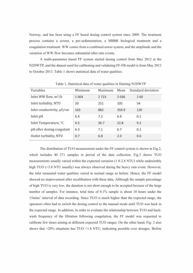
Norway, and has been using a FF based dosing control system since 2009. The treatment

process contains a screen, a pre-sedimentation, a MBBR biological treatment and a

coagulation treatment. WW comes from a combined sewer system, and the amplitude and the

variation of WW flow becomes substantial after rain events.

A multi-parameter based FF system started dosing control from May 2012 at the

N2DWTP, and the dataset used for calibrating and validating FF-FB model is from May 2012

to October 2013. Table 1 shows statistical data of water qualities.

Table 1, Statistical data of water qualities in Haining N2DWTP

The distribution of TUO measurement under the FF control system is shown in Fig.2,

which includes 40 271 samples in period of the data collection. Fig.2 shows TUO

measurements usually varied within the expected variation (1.8-2.8 NTU) while undesirably

high TUO (>3.8 NTU usually) was always observed during the heavy rain event. However,

the inlet measured water qualities varied in normal range as before. Hence, the FF model

showed no improvement after recalibration with these data. Although the sample percentage

of high TUO is very low, the duration is not short enough to be accepted because of the large

number of samples. For instance, total time of 0.1% sample is about 10 hours under the

15mins’ interval of data recording. Since TUO is much higher than the expected range, the

operators often had to switch the dosing control to the manual mode until TUO was back in

the expected range. In addition, in order to evaluate the relationship between TUO and back-

wash frequency of the filtration following coagulation, the FF model was requested to

calibrate few times aiming at different expected TUO ranges. On the other hand, Fig. 2 also

shows that >20% situations has TUO <1.8 NTU, indicating possible over dosages. Before

calibrating FF-FB models for Haining N2DWTP, the set point in Equation (3) is fixed to

TUO=2.3 NTU according to the plant’s usual desired value.

Figure 2, Distribution of outlet turbidity measurement under feedforward system

control in Haining number two drinking water treatment plant.

The dataset from NRA during December 2013 to December 2014 was used for the

analysis presented here. The set point is fixed to TUO=3.0 NTU as usual desired value. The

statistical data is shown in Table 2.

Table 2, Statistical data of water qualities in NRA WWTP

Fig.3 shows distribution of TUO measurement during the dosing control using the FF

model at NRA and the figure is based on 32 124 data points. The expected TUO range is 1-4

NTU. It is also observed that 25% TUO measurements were beyond the expected range, in

which 18.4% TUO measurement is higher than 4 NTU especially when inlet WW flow is

varying in high level.

Outlet Turbidity (TUO) measurement range,

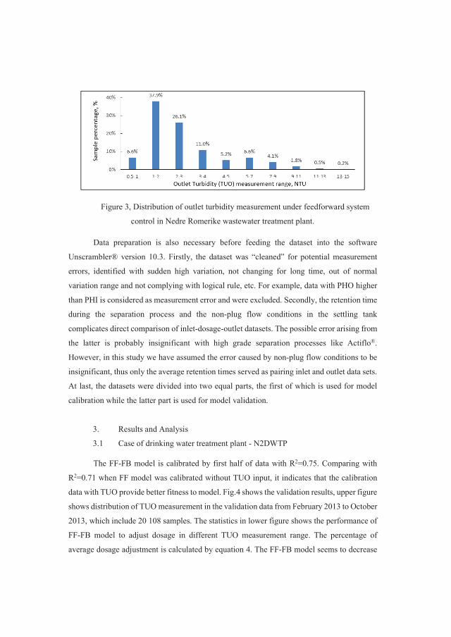
Figure 3, Distribution of outlet turbidity measurement under feedforward system

control in Nedre Romerike wastewater treatment plant.

Data preparation is also necessary before feeding the dataset into the software

Unscrambler® version 10.3. Firstly, the dataset was “cleaned” for potential measurement

errors, identified with sudden high variation, not changing for long time, out of normal

variation range and not complying with logical rule, etc. For example, data with PHO higher

than PHI is considered as measurement error and were excluded. Secondly, the retention time

during the separation process and the non-plug flow conditions in the settling tank

complicates direct comparison of inlet-dosage-outlet datasets. The possible error arising from

the latter is probably insignificant with high grade separation processes like Actiflo®.

However, in this study we have assumed the error caused by non-plug flow conditions to be

insignificant, thus only the average retention times served as pairing inlet and outlet data sets.

At last, the datasets were divided into two equal parts, the first of which is used for model

calibration while the latter part is used for model validation.

3. Results and Analysis

3.1 Case of drinking water treatment plant - N2DWTP

The FF-FB model is calibrated by first half of data with R2=0.75. Comparing with

R2=0.71 when FF model was calibrated without TUO input, it indicates that the calibration

data with TUO provide better fitness to model. Fig.4 shows the validation results, upper figure

shows distribution of TUO measurement in the validation data from February 2013 to October

2013, which include 20 108 samples. The statistics in lower figure shows the performance of

FF-FB model to adjust dosage in different TUO measurement range. The percentage of

average dosage adjustment is calculated by equation 4. The FF-FB model seems to decrease

the predicted dosage when TUO < 2.3 NTU (set point), while the dosage increases when

TUO> the set point. Furthermore, degree of this adjustment is increasing when TUO becomes

further away from the set point. In case of TUO > 3.8 NTU, dosage of the FF model could

not adjust the adequately and the TUO starts to increase. Then the plant operators switched to

original flow-proportional dosing control, which is manually -adjusted the dosage. Otherwise,

the dosage adjustment of the FF-FB model should be approximately shown as dot line bars in

range of 3.8-5.8 NTU.

Equation (4)

Therefore, the FF model after adding a FB variable seems able to compensate for

variations of the inlet qualities, resulting in more stable TUO.

Figure 4, Statistics on validation result of feedforward-feedback model in Haining

Number two drinking water treatment plant

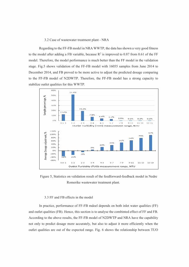
3.2 Case of wastewater treatment plant - NRA

Regarding to the FF-FB model in NRA WWTP, the data has shown a very good fitness

to the model after adding a FB variable, because R2 is improved to 0.87 from 0.61 of the FF

model. Therefore, the model performance is much better than the FF model in the validation

stage. Fig.5 shows validation of the FF-FB model with 16055 samples from June 2014 to

December 2014, and FB proved to be more active to adjust the predicted dosage comparing

to the FF-FB model of N2DWTP. Therefore, the FF-FB model has a strong capacity to

stabilize outlet qualities for this WWTP.

Figure 5, Statistics on validation result of the feedforward-feedback model in Nedre

Romerike wastewater treatment plant.

3.3 FF and FB effects in the model

In practice, performance of FF-FB mdoel depends on both inlet water qualities (FF)

and outlet qualities (FB). Hence, this section is to analyse the combinted effect of FF and FB.

According to the above results, the FF-FB model of N2DWTP and NRA have the capability

not only to predict dosage more accurately, but also to adjust it more efficiently when the

outlet qualities are out of the expected range. Fig. 6 shows the relationship between TUO

deviation from set-point (A-axis, presented by Equation 6) and dosage adjustment percentage

(Y-axis, presented by Equation 5). If the pure FB control of dosage, the relationship between

dosage adjustment percentage and TUO deviation from set-point should be a strict line like

y=ax. In order to show the relationship with small amount of samples, Fig.6a and 6b contain

10% of total samples respectively, which are random-selected.

Y-axis: Dosage adjustment percentage = (Dosage of FF-FB model - real Dosage)/ real

Dosage*100% Equation (5)

X-axis: Outlet deviation=Outlet measurement - Set point Equation (6)

Fig. 6a is from N2DWTP and Fig. 6b is from NRA WWTP. The relationship between

outlet quality deviation and dosage adjustment is not as linear as the strict line (y=ax). This

indicates that strengths of the dosage adjustment are not identical when the same TUO

deviations from the set point happen. This is because inlet water qualities are different even

under the same TUO deviations, which should generate vairous FF contributions to dosage

prediction and differ the strengths of the dosage adjustment. Thus, the relationship in Fig. 6a

and 6b pressent as the shape of a belt but not the strict line.

Figure 6, Relationship between outlet quality deviation from set-point and

dosage adjustment percentage. (Dosage adjustment percentage = (dosage prediction-real

dosage)/real dosage*100%, a. part is from Haining Number two drinking water

treatment plant and b. part is from Nedre Romerike wastewater treatment plant.

3.4 Changes on coagulant consumption

Since the FF-FB model is able to adjust dosage to constant TUO, the coagulant

consumption will be changed accordingly. Based on statistics data in Table 4 and 5, this

a.

section estimates potential changes on coagulant consumption under the FF-FB model

control. In Table 4, the pump frequency as the system output is an indictor to coagulant flow,

which is proportional to the coagulant dosing flow. For N2DWTP, during the period of

validation (9 months), the FF-FB model used 3.7 % less coagulants to prevent over-dosage.

However, the overall coagulant consumption with the FF-FB model to secure more stable

TUO was 2.6% more than the FF model, because 12 809 data points originally had an under-

dosage resulting in TUO>2.3. Whereas in NRA the total consumption of the FF-FB model

became less, which could save 9.2% coagulant during the validation period (6 months). If the

FB-FF model’s task only was to reduce the over-dosage, the savings would be 15.5%.

Therefore, if inlet qualities are similar to validation data and TUO can work as a non-delayed

FB variable, the FF-FB model can provide approximately 9.2% coagulant savings in future

applications.

Table 4, parameters of changes on coagulant consumption in Haining N2DWTP

Table 5, parameters of changes on coagulant consumption in NRA WWTP

4. Conclusions and Discussions

TUO measurement range, NTU 0.8-1.3 1.3-1.8 1.8-2.3 2.3-2.8 2.8-3.3 3.3-3.8 3.8-5.8

Sample percentage, % 0.2% 4.7% 31.3% 46.6% 14.0% 1.8% 1.3%

Average Dosage adjustment, % -19% -16% -10% 7% 19% 20% 4%

Average pump frequency, Hz 26.81 25.19 24.46 24.91 25.21 26.83 36.88

The options for the use of Feed-Forward (FF) and Feed-Forward combined with Feed-

Back (FF-FB) were discussed.

A concept to integrate the FB values to the existing FF models was presented. The

results of dosing control strategies based on the FB-FF models were superior to strategies

based on the FF-models. The increased efficiency of the model were documented with data

from full-scale tests both from drinking water and wastewater treatment plants.

The FF-FB models generated algorithms with better qualities compared with the FF

only models. If the objective of the FF-FB model based control was only to avoid over dosage,

it is possible to achieve savings in the range of 3.7-15.5%.

The possibility to generate more stable outlet qualities with the FF-FB model based

controls were demonstrated. The outlet qualities became more stable but the overall coagulant

consumption became only 9% less in WWTP while it increased by 3% in N2DWTP. The

latter was a result of longer periods with under dosage leading to poor outlet qualities, and an

increase in dosage was often required to produce better and consistent outlet qualities.

Since the empirical model has a strong ability to establish the relationship among

variables from historical data, the model performance can be improved by the data with more

accurate dosages. Considering the common retention time of sedimentation tanks and the

associated internal mixing may be a challenge. However, a simplifications applied in this

study shows a significant trend to improve the outlet quality. With reduced retention times in

separation stages, the model accuracy will obviously be better as it can include measured

outlet values in the models. Another solution could be the use of FF based soft sensors for

outlet qualities, enabling the use of the FF-FB models in the separation stages with longer

retention times (Liu and Ratnaweera 2015). However, the FF-FB model can still apply to

DWT plants because inlet quality changes are often scaled by hours and days rather than

minutes in most cases. The model could also apply to WWTP with high rate settling tanks

such as lamella, Actiflo etc., which reduce the settling time from hours to minutes.

Acknowledgement: Authors appreciate the assistance provided by Haining N2DWTP,

NRA WWTP, and DOSCON Co Ltd. (www.doscon.no) for providing access to the multi-

parameter based dosing control system.

Reference

Ashraf A. & Barry L. 2009, ‘Model predictive control monitoring using multivariate statistics’, Journal of Process, vol. 19, no.2, pp. 314-327

Baxter CW., Shariff R., Stanley SJ., Smith DW., Zhang Q. & Saumer ED. 2002, ‘Model-based advanced process control of coagulation’, Water Science and Technology, vol. 45, no. 4-5, pp. 9-17

Chu JZ., Jang SS., & Chen YN. 2004, ‘A Comparative Study of Combined Feedforward/Feedback Model Predictive Control for Nonlinear Systems’, Canadian Journal of chemical Engineering, vol. 82, pp. 1-10

Dayal, BS. & MacGregor, JF. 1997, ‘Improved PLS algorithms’, J. Chemometrics, vol.11, no.1, pp: 73-85

Dentel SK. and Abu-Orf MM. 1995, ‘Laboratory and full-scale studies of liquid stream viscosity and streaming current for characterization and monitoring of dewaterability’, Water Research, vol.29, no.12, pp: 2663-2672

Liu W., Ratnaweera H. & Song HP. 2013, ‘Better treatment efficiencies and process economies with real-time coagulant dosing control’, 11th IWA conference on instrumentation control and automation, France

Liu W. & Ratnaweera H. 2015, ‘Feed-forward based software-sensor for outlet turbidity of coagulation process’ (in preparation)

Ingildsen P., Jeppsson U. & Olsson G. 2002, ‘Dissolved oxygen controller based on on-line measurements of ammonium combining feed-forward and feed-back’, Water Science and Technology, vol. 45, no.4-5, pp. 453-460

Maier HR., Jain A., Dandy GC. & Sudheer KP. 2010, ‘Methods used for the development of neural networks for the prediction of water resource variables in river systems: Current status and future directions’, Environmental Modelling & Software vol. 25, no. 8, pp. 891-909

Ogata K. 2010 ‘Modern control engineering’, Fifth Edition, Pearson Education, New Jersey Rathnaweera S. 2010 ‘Modelling and optimization of wastewater coagulation process’, PhD

thesis, Dept. of Mathematical Sciences and Technology, Norwegian University of Life Sciences, Aas, Norway

Ratnaweera H., Smoczy ski L. & Lewandowski A. 2005, ‘Efficient coagulant dosing in wastewater treatment’, Problems and Progress in Agricultural Sciences, Polish Academy of Sciences, vol. 505, pp. 347-352

Ratnaweera H., and Fettig J. 2015, ‘State of the art of online monitoring and control of the coagulation process’, Water, vol.7, pp:6574-6597

Stanley, SJ., Baxter C.W. and Zhang, Q., 2000, Process Modelling and Control of Enhanced Coagulation, AWWA Research Foundation, Washington DC, USA

Vrecko D., Havla N. & Carlson B. 2003, ‘Feedforward-feedback control of an activated sludge process: a simulation study’, Water Science and Technology, vol. 47, no. 12, pp: 19-26

Yu FR., Kang SF., Liaw SL. & Chen MC. 2000, ‘Application of artificial neural network to control the coagulant dosing in water treatment plant’, Water Science and Technology, vol. 42, no. 3-4, pp. 403-408

Zeng GM., Qin XS., He L., Huang GH., Liu LH. & Lin YP. 2003, ‘A neural network predictive control system for paper mill wastewater treatment’, Engineering Application of Artificial Intelligence, vol. 16, no.2, pp. 121-129

Paper III

Feed-forward based software sensor for outlet turbidity of coagulation process

Liu Wei, Ratnaweera Harsha

The paper is submitted to International Journal of Research & Development

Organization

1

*

Variables Minimum Maximum

Mean Standard deviation

Inlet WW flow, m3/h 108.5 1466.3 643.7 294.4

TUI, NTU 41.7 411.1 101.7 32.9

CNI, S/cm 170.9 983.2 473.1 110.0

PHI 5.9 6.8 6.4 0.1

TMP, °C 7.6 22.0 15.6 3.6

PHO 5.3 6.7 6.1 0.2

TUO, NTU 0.5 14.9 2.8 2.1

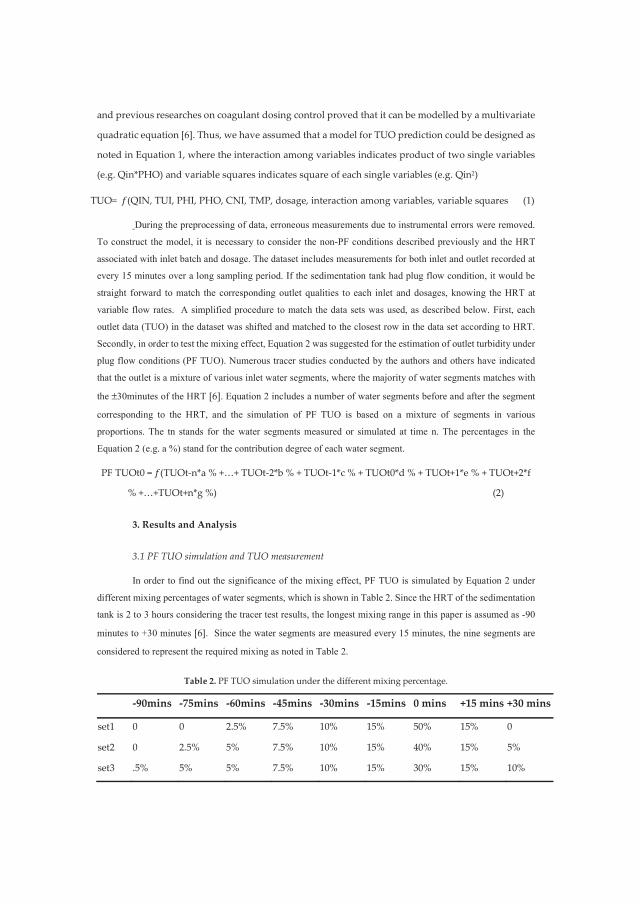
During the preprocessing of data, erroneous measurements due to instrumental errors were removed.

To construct the model, it is necessary to consider the non-PF conditions described previously and the HRT

associated with inlet batch and dosage. The dataset includes measurements for both inlet and outlet recorded at

every 15 minutes over a long sampling period. If the sedimentation tank had plug flow condition, it would be

straight forward to match the corresponding outlet qualities to each inlet and dosages, knowing the HRT at

variable flow rates. A simplified procedure to match the data sets was used, as described below. First, each

outlet data (TUO) in the dataset was shifted and matched to the closest row in the data set according to HRT.

Secondly, in order to test the mixing effect, Equation 2 was suggested for the estimation of outlet turbidity under

plug flow conditions (PF TUO). Numerous tracer studies conducted by the authors and others have indicated

that the outlet is a mixture of various inlet water segments, where the majority of water segments matches with

the ±30minutes of the HRT . Equation 2 includes a number of water segments before and after the segment

corresponding to the HRT, and the simulation of PF TUO is based on a mixture of segments in various

proportions. The tn stands for the water segments measured or simulated at time n. The percentages in the

Equation 2 (e.g. a %) stand for the contribution degree of each water segment.

In order to find out the significance of the mixing effect, PF TUO is simulated by Equation 2 under

different mixing percentages of water segments, which is shown in Table 2. Since the HRT of the sedimentation

tank is 2 to 3 hours considering the tracer test results, the longest mixing range in this paper is assumed as -90

minutes to +30 minutes . Since the water segments are measured every 15 minutes, the nine segments are

considered to represent the required mixing as noted in Table 2.

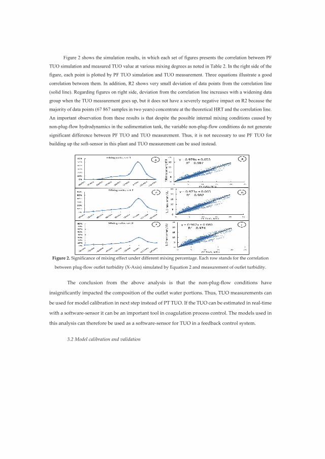
Figure 2 shows the simulation results, in which each set of figures presents the correlation between PF

TUO simulation and measured TUO value at various mixing degrees as noted in Table 2. In the right side of the

figure, each point is plotted by PF TUO simulation and TUO measurement. Three equations illustrate a good

correlation between them. In addition, R2 shows very small deviation of data points from the correlation line

(solid line). Regarding figures on right side, deviation from the correlation line increases with a widening data

group when the TUO measurement goes up, but it does not have a severely negative impact on R2 because the

majority of data points (67 867 samples in two years) concentrate at the theoretical HRT and the correlation line.

An important observation from these results is that despite the possible internal mixing conditions caused by

non-plug-flow hydrodynamics in the sedimentation tank, the variable non-plug-flow conditions do not generate

significant difference between PF TUO and TUO measurement. Thus, it is not necessary to use PF TUO for

building up the soft-sensor in this plant and TUO measurement can be used instead.

•

•

•

•

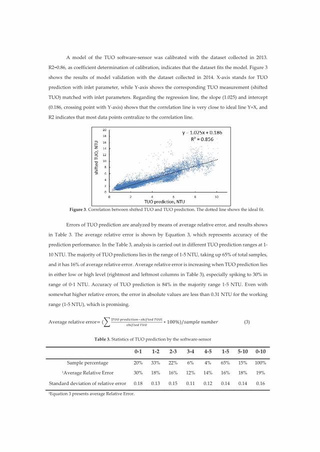
Paper IV

Model-based measurement error detection of coagulant dosage control system

Liu Wei, Ratnaweera Harsha, Knut Kvaal

The paper is submitted to International Journal of Environmental Science and

Technology

Model-based measurement error detection of a coagulant

dosage control system

Wei Liu1*, Harsha Ratnaweera12 and Knut Kvaal13

1 Norwegian University of Life Sciences, PO Box 5003-IMT, 1432 Aas, Norway.

*Author to whom correspondence should be addressed; E-Mail: wei.liu@nmbu.no; Tel.: +47-9396-

4044. 2 E-Mail: harsha.ratnaweera@nmbu.no 3 E-Mail: knut.kvaal@nmbu.no

Abstract: Online instruments are widely used in wastewater treatment plants and drinking water

treatment plants for process monitor and control. Although maintenances of online sensors are

important routine works, potential measurement errors of online sensors are challenging not only

monitoring of coagulation process but also coagulant dosage control system, what this paper is

focusing on. In order to estimate and detect the potential measurement error, this paper proposes a

concept of model-based measurement error detection. Based on the concept, this paper enables to

quantify the measurement errors and build up a novel detection method. In addition, the paper

compares the proposed detection method with a traditional method-the normal variation range. The

results show that the proposed method has a better efficiency to detect the measurement error.

Keywords: Error detection; model; coagulation, online sensors, normal distribution

1. Introduction

In order to monitor, simulate and control wastewater treatment and drinking water treatment,

online sensors are widely used. Relying on the online sensors, performance of each treatment section

can be monitored and corresponding operations can be carried out in time. Hence, measurement

accuracy of online sensors is very important to process monitor and control. Although online sensors

are regularly maintained, the measurement errors occur frequently (Thomann et al., 2002).

Consequently, the measurement errors lead to inaccurate or even wrong operation, which could result

in poor treatment efficiency and high operation costs. Accuracy of online measurements is still a weak

point in the control chain (Winkler et al., 2004; Rieger et al., 2005; Rieger and Vanrolleghem, 2008).

Therefore, the detection method of online measurement errors is necessary to study.

1.1 Background

In wastewater treatment plants (WWTPs) and drinking water treatment plants (DWTPs),

measurement errors of online sensors generate by several reasons. Firstly, particles, grease and

crystallized coating tend to stick on sensor surface, which hinders the sensors to touch with

wastewater. Secondly, aging issue causes unstable working status and measurement deviation from

true value. Thirdly, due to the communication interruption between online sensors and the plant

control system, the measurement values cannot be updated. Fourthly, human mistakes such as

inaccurate calibration and wrong settings also result in the measurement errors. In practice, since inlet

water quality continually changes with time, the measurement errors in the variation curve show as

different styles such as peak, constant, and drift.

Detection methods of the measurement errors are comprehensively studied, which are divided

into two categories in general. Model-free approach focuses on single parameter measurement instead

of considering the correlation among multiple parameters. Because of simple implementation, the

model free approach such as normal distribution, discordant test and Rosner test are widely used

(Rosner, 1983; Edward and Charles, 2014). Model based approach is to detect whether the correlation

among many parameters are either statistically correct or in agreement with chemical or physical

properties of the system (Robinson et al, 2005; Lo et al., 2016). Regarding the model-based approach,

the empirical model are becoming popular for measurement error detection and several methods prove

to be useful such as Artificial Neural Network (ANN), Partial Least Square Regression (PLSR) and

Principal Component Analysis (PCA) (MacGregor et al., 1994; Luo et al., 1999

Venkat et al., 2003).

The coagulation process, what this paper is focusing on, is a multivariate non-linear system

(Rathnaweera, 2010; Maier et al., 2010). The outlet quality of coagulation process, taking wastewater

treatment as example, highly depends on coagulant dosage and inlet parameters including pH,

turbidity, phosphate, temperature and so on. In order to achieve expected outlet quality (controlled

variable), coagulant dosage as a key manipulated variable should be close to optimum value to deal

with rapidly changeable inlet quality (disturbing variables) (Liu and Ratnaweera, 2016a). In other side,

erroneous online measurements of inlet quality leading to inaccurate the dosage prediction cause

unexpected outlet quality. Hence, outlet quality highly is dependent on working status of these inlet

sensors when the coagulant dosage control system is running. In practice, although routine

maintenances (clean and calibration) are regularly carried out by plant workers, measurement errors

of online sensors usually occur and are challenging the reliability of the dosage control system. Thus,

the error detection of inlet measurements is very necessary for a multi-parameter dosage control

system.

Modelling of coagulant dosage control has been widely studied (Maier et al., 2004;

Ratnaweera and Fettig, 2015). Since there has been no a conceptual model so far due to the complexity

of coagulation process, relationships between inlet parameters, dosage and outlet parameters are

generally expressed by empirical models (Ratnaweera and Fettig, 2015). Since the empirical models

are derived from large number of historical data instead of chemical and physical properties of

coagulation process, the equation embedded in empirical model is difficult to be explained by

chemical and physical knowledge (Maier et al., 2000). A multi-parameter dosage control system, using

PLSR as the method of model calibration, was tested and applied in many WWTPs and DWTPs

achieving acceptable results (Rathnaweera, 2010; Liu et al., 2013). Equation 1 presents model

structure of the multi-parameter dosage control system. By receiving online signals including

wastewater flow (QIN), inlet pH (PHI), inlet turbidity (TUI), pH after coagulation (PHO), inlet

conductivity (CNI), temperature (TMP) and outlet turbidity (TUO), the control system calculates real-

time coagulant dosage. Hence, basing on the modelling method and the model structure, this paper is

to develop a model-based measurement error detection for the coagulant dosage control system.

Dosage prediction = (QIN, TUI, PHI, PHO, CNI, TMP, TUO, interaction among variables,

variables squares) Equation (1)

Lo et al. (2016) pointed out that the process of sensor fault diagnosis can be classified into

four steps: (1) detection (detecting whether there are any faulty sensors in the system), (2) isolation

(determining which sensor(s) is (are) faulty), (3) identification (determining the type of faults that

occurred) and (4) recovery (estimating the correct output of the faulty sensors). The model-based

measurement error detection, what this paper proposes, belongs to the first step of the sensor fault

diagnosis.

1.2 Concept of the proposed error detection

Reference is a key factor of the proposed error detection in this paper. Since outlet quality

measured by outlet sensors indicates the treatment performance, outlet sensors has importance role in

coagulation process. Hence, this paper uses outlet sensor as the reference sensor of the proposed error

detection. In practice, in order to ensure working status of outlet online measurements, online sensors

are sometimes double or triple installed at process outlet so that difference between them can reveal

the potential measurement error. Furthermore, in order to check the accuracy of outlet online

measurements, laboratory measurements of grasping samples are often compared with online

measurements. Moreover, much better working environment at the process outlet, where most

particles settled down, reduces error possibilities of outlet sensors. Therefore, outlet sensors are some

of the most reliable instruments in the dosage control system, which is able to function as the reference

sensor of the error detection of inlet measurement. Since the coagulation process as testing field of

this paper is using turbidity to indicate outlet quality, the outlet turbidity sensor (TUO) is consider as

the reference sensor.

Based on the TUO software sensor as the result of authors’ previous research (Liu and

Ratnaweera, 2016b), it enables to simulate TUO at given inlet parameters and dosage. Hence, there

are differences between TUO measurements and corresponding TUO simulations. This paper

considers that these differences are caused by both model errors and inlet measurement errors. Model

errors are related to model accuracy, which causes unpredictable fluctuations of TUO simulation. This

paper is to prove model errors repeat within a certain range and the related differences caused by the

fluctuations are limited to the certain range. Thus, the proposed concept of the error detection is that

when the differences exceed the certain range what model errors decided, the measurement errors of

inlet sensors are considered to happen. Figure 1 describes the above concept, where dotted lines

indicate sources of differences.

Figure 1. Concept of error detection of inlet measurements, dotted lines indicate sources of

difference

1.3 Objectives and research procedure

Based on the TUO simulation model, this paper aims to i) define the difference range what is

caused by model error, ii) build up a detection criterion for inlet measurement errors, iii) compare the

proposed method with a traditional method-normal variation range what the current dosage control

system is using. The research is carried out by following procedure. Firstly, operation data was

collected from a full-scale coagulation process, measurement errors of each parameter are defined by

traditional method referring to the normal distribution and these errors of each parameter are marked

in dataset. Secondly, based on previous research on the TUO simulation model (Liu and Ratnaweera,

2016), TUO simulation model is calibrated with the dataset including the marked errors. Thirdly,

analyze the deviation of TUO simulations and define the range of model errors. At last, build up a

criterion of the error detection and compare it with the traditional method.

2. Materials and methods

The operation data was collected in Nedre Romerike (NRA) WWTP, located in Lillestrom

Norway. The capacity is 110 000 PE. and treatment process consists of a screen, a pre-sedimentation,

Inlet Measurements Model

TUO Simulation

DifferenceInlet measurement errors, if the difference is outside the certain range

NO inlet measurement error, if the difference is within the certain range.

Dosage

a MBBR biological treatment and a coagulation treatment. Figure 2 shows schematic of the treatment

process. The coagulation process includes two treatment lines in parallel. Inlet sensors mentioned

above are installed in one of lines before the coagulant dosing pump, the PHO sensor lies in the

flocculation chamber as a section of coagulation process, and one of two TUO sensors is installed at

the end of one line and another is installed at the outlet of the process where these two parallel lines

join. Online measurement signals are sent to supervisory control and data acquisition (SCADA,

WWTP control system) at first and then transfer to the dosing control system by means of Modbus

communication. These measurement signals are recorded at 15 minutes’ interval and there is no time

delay during the signal transferring. Normally, these online sensors are maintained once per week.

The operation data was collected from January 2013 to December 2014.

Figure 2, Schematic of treatment process in NRA WWTP, dash lines indicate the location of device

and online sensors

The current dosage control system contains two criteria as the error detection of inlet

measurements. The first criterion is to define whether inlet measurement values are within the normal

range. Variation checking, as the second criterion, is to detect whether each sensor is active to work

or signal communication pauses. Both two criteria belong to the univariate approach, which is used to

compared with the proposed error detection method.

The normal variation range is determined by referring to standard deviation of measurements,

mean value and historical observations. Based on the operation data, Figure 3 shows measurement

distribution of each parameter. Total amount of samples is 67 872. Height of each bar indicates

occurrence frequency within the total amount. Table 1 shows the normal range of each parameter.

Some measurements with short bar, lying outside of the normal variation range, are identified as inlet

measurement errors. Those errors defined by the normal variation range are marked in the dataset. The

research in this paper is carried out with the operation data.

Grit chamber

Primary settling tank

Biological treatment

Coagulation process

Coagulant Dosing pump

Sludge treatment Sludge disposal

Sludge disposal

Inlet sensors

Outlet sensors

Influence Effluent

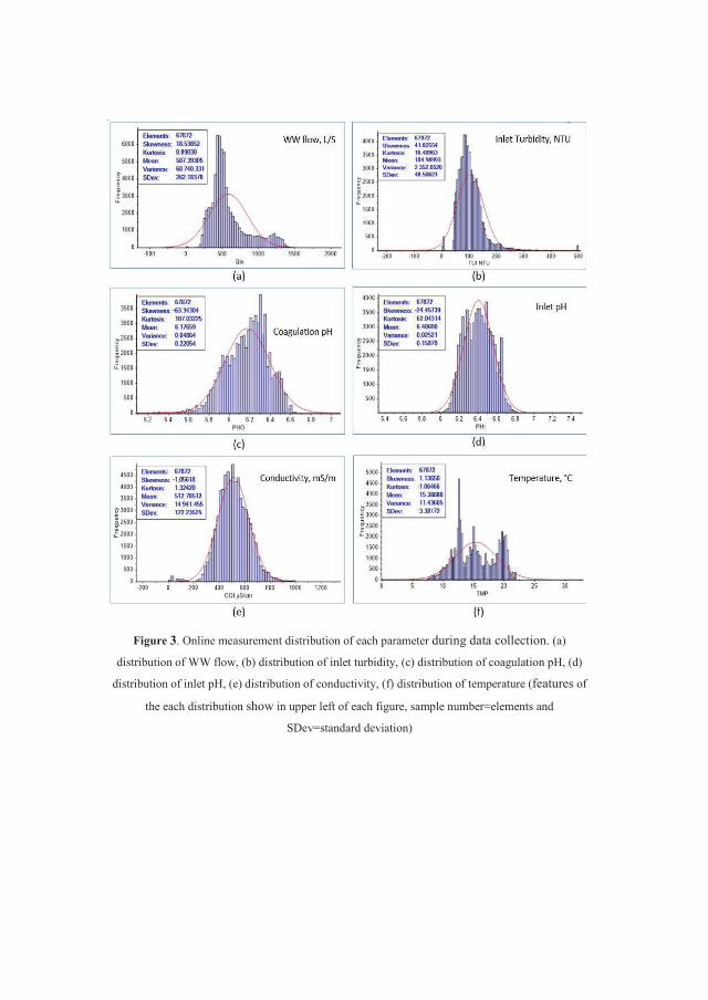
Figure 3. Online measurement distribution of each parameter during data collection. (a)

distribution of WW flow, (b) distribution of inlet turbidity, (c) distribution of coagulation pH, (d)

distribution of inlet pH, (e) distribution of conductivity, (f) distribution of temperature (features of

the each distribution show in upper left of each figure, sample number=elements and

SDev=standard deviation)

Table 1. Normal variation range of each parameter

PARAMETER QIN, L/S PHI TUI, NTU CNI, MS/M TMP, °C PHO

Partial Least square Regression (PLSR), as method of model calibration, applies to build up

the relationship among TUO, inlet parameters and dosages. The model structure is shown as Equation

2, where interactions among variables mean to product of two inlet parameters (e.g. Qin*PHO) and

squares are responsible for the non-linear relationship. PLSR is carried out by Software Unscrambler®

(version 10.3). Considering retention time of sedimentation tank, TUO measurements are not results

of inlet parameters and dosages, which are recorded at the same time and written in the same row of

dataset. Thus, before inputting the collected dataset in the software, TUO measurements are shifted

and matched to inlet parameters considering the hydraulic retention time.

TUO prediction = (QIN, TUI, PHI, PHO, CNI, TMP, dosage, interaction among variables,

variables squares) Equation (2)

3. Results and discussions

The TUO simulation model was calibrated by the above concept and method, which enables

to simulate TUO with given inlet parameters and dosage. Since random sample indicates that each

individual sample has same possibility to be selected, it has advantage of avoiding classification

interruption such as sampling time and data duration (Yates et al., 2008). Hence, in order to check

stability of model errors, certain amount of random samples are selected from total samples (67 872)

for the model calibration. Table 2 shows statistics results of five models. Four of them are calibrated

with different 5000 samples that are randomly selected from total samples, whereas one of them

is calibrated with total samples. The results show that there are small variations among these

five models. This not only indicates that the relationship among inlet parameters, dosage and TUO

is quite constant when models are calibrated with different small amount of data, but also results of

root mean square error (RMSE) reveal that model errors are so stable that the proposed method of

error detection can rely on. Due to small variations among these five models, model 4 is

selected to display the performance of TUO simulation, which is shown in figure 4 and plotted

with TUO simulations and TUO measurements. Equation 3 represents the correlation line (black line)

between TUO simulations (TUOs, shown as predicted Y on Y-axis in figure 4) and TUO

measurements (TUOm, shown as reference Y on X-axis figure 4), which is used for detection

criterion in chapter 3.2.

Table 2. Statistics of outlet turbidity simulation models with different sample selections

parameter Model 1

with 5000

random-

selected

sample

Model 2

with 5000

random-

selected

sample

Model 3 with

5000

random-

selected

sample

Model 4 with

5000

random-

selected

sample

Model 5 with

whole

samples

R2 0.817 0.823 0.823 0.817 0.814

slope 0.817 0.825 0.817 0.823 0.814

Offset 0.426 0.404 0.406 0.406 0.431

RMSE1 0.727 0.716 0.732 0.733 0.732 1 RMSE is abbreviation for Root Mean Square Error. Model with 5000 random-selected samples is

able to show constant results, comparing with 50 or 500 random-selected samples.

Figure 4. Correlation between simulations and measurements of outlet turbidity, black line presents

the correlation line.( Sample number=elements, Slope, Offset, R2= coefficient of determination and

RMSE=root mean square error as main parameters of the correlation line list in the upper left of the

figure)

TUOs=Slope*TUOm + Offset (3)

3.1 Defining the range of model errors

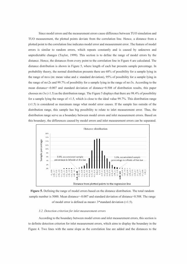
Since model errors and the measurement errors cause difference between TUO simulation and

TUO measurement, the plotted points deviate from the correlation line. Hence, a distance from a

plotted point to the correlation line indicates model error and measurement error. The feature of model

errors is similar to random errors, which repeats constantly and is caused by unknown and

unpredictable changes (Taylor, 1999). This section is to define the range of model errors by the

distance. Hence, the distances from every point to the correlation line in Figure 4 are calculated. The

distance distribution is shown in Figure 5, where length of each bar presents sample percentage. In

probability theory, the normal distribution presents there are 68% of possibility for a sample lying in

the range of m±s (m: mean value and s: standard deviation), 95% of possibility for a sample lying in

the range of m±2s and 99.7% of possibility for a sample lying in the range of m±3s. According to the

mean distance=-0.007 and standard deviation of distance=0.508 of distribution results, this paper

chooses m±3s (±1.5) as the distribution range. The Figure 5 displays that there are 98.4% of possibility

for a sample lying the range of ±1.5, which is close to the ideal value 99.7%. This distribution range

(±1.5) is considered as maximum range what model error causes. If the sample lies outside of the

distribution range, this sample has big possibility to relate to inlet measurement error. Thus, the

distribution range serve as a boundary between model errors and inlet measurement errors. Based on

this boundary, the differences caused by model errors and inlet measurement errors can be separated.

Figure 5. Defining the range of model errors based on the distance distribution. The total random

sample number is 5000. Mean distance=-0.007 and standard deviation of distance=0.508. The range

of model error is defined as mean± 3*standard deviation (±1.5).

3.2. Detection criterion for inlet measurement errors

According to the boundary between model errors and inlet measurement errors, this section is

to definite detection criterion for inlet measurement errors, which aims to display the boundary in the

Figure 4. Two lines with the same slope as the correlation line are added and the distances to the

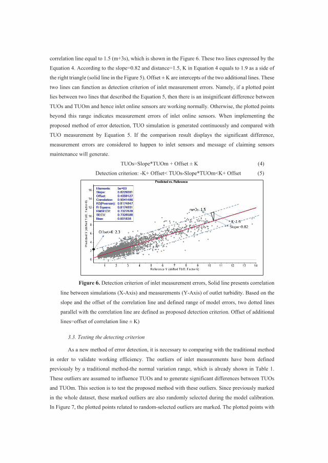
correlation line equal to 1.5 (m+3s), which is shown in the Figure 6. These two lines expressed by the

Equation 4. According to the slope=0.82 and distance=1.5, K in Equation 4 equals to 1.9 as a side of

the right triangle (solid line in the Figure 5). Offset ± K are intercepts of the two additional lines. These

two lines can function as detection criterion of inlet measurement errors. Namely, if a plotted point

lies between two lines that described the Equation 5, then there is an insignificant difference between

TUOs and TUOm and hence inlet online sensors are working normally. Otherwise, the plotted points

beyond this range indicates measurement errors of inlet online sensors. When implementing the

proposed method of error detection, TUO simulation is generated continuously and compared with

TUO measurement by Equation 5. If the comparison result displays the significant difference,

measurement errors are considered to happen to inlet sensors and message of claiming sensors

maintenance will generate.

TUOs=Slope*TUOm + Offset ± K (4)

Detection criterion: -K+ Offset< TUOs-Slope*TUOm<K+ Offset (5)

Figure 6. Detection criterion of inlet measurement errors, Solid line presents correlation

line between simulations (X-Axis) and measurements (Y-Axis) of outlet turbidity. Based on the

slope and the offset of the correlation line and defined range of model errors, two dotted lines

parallel with the correlation line are defined as proposed detection criterion. Offset of additional

lines=offset of correlation line ± K)

3.3. Testing the detecting criterion

As a new method of error detection, it is necessary to comparing with the traditional method

in order to validate working efficiency. The outliers of inlet measurements have been defined

previously by a traditional method-the normal variation range, which is already shown in Table 1.

These outliers are assumed to influence TUOs and to generate significant differences between TUOs

and TUOm. This section is to test the proposed method with these outliers. Since previously marked

in the whole dataset, these marked outliers are also randomly selected during the model calibration.

In Figure 7, the plotted points related to random-selected outliers are marked. The plotted points with

various shapes represent different inlet parameters. It can be seen that these random-selected outliers

do not always result in the obvious difference. Taking square points (related to inlet turbidity outliers)

as an example, some square points close to the correlation line indicate small influence to TUOs while

some square points far from the line generate the large influence. Other points with different shapes

also have such situation. Therefore, the results of proposed detection criterion is not fully in

accordance with the traditional method-the normal variation range.

This inconsistency is analyzed below. According to the TUO simulation model shown as

Equation 2, any single parameter has two ways to contribute TUOs. Firstly, the direct contribution is

carried out by the single parameter. Secondly, interactions among variables are combined

contributions with two parameters (e.g. PHO *dosage in equation 2). This combined contribution

could become insignificant when one of two parameters is varying in low level, whereas the combined

contribution could be significant when both parameters are varying in high level. Hence, a difference

between a TUOs and a TUOm depends on whether a parameter with the measurement error has a

significant influence. If an insignificant influence leads to the unobvious difference between TUOs

and TUOm, then it is unnecessary to identify the inlet measurement errors under such situation.

Therefore, the traditional method of normal variation range focuses on sensor itself and could work

universally but not as efficiently as the proposed method. The proposed detection method is only to

identify the measurement error, which tends to deviate TUOs from TUOm.

Figure 7. Comparison of proposed detection method and the traditional method (this

figure bases on the correlation between simulation and measurements of outlet turbidity, solid

line presents the correlation line and two dotted lines indicate proposed detection criterion of

measurement errors, various points marked by difference shapes are measurement errors defined

by the traditional method)

4. Conclusions

In order to detect potential inlet measurement errors for the coagulant dosage control system,

a concept of model-based measurement error detection is proposed in this paper. This concept is

implemented by the differences between measurements and simulations of outlet turbidity. This paper

considers that the differences are caused by model errors and inlet measurement errors. If the

differences are outside of the range what model errors decided, then inlet measurement errors are

considered to happen. The concept proved to be effective based on results. And following conclusions

can be drawn.

• The model error of the multi-parameter dosage control system can be quantified by the

difference between simulation and measurement of outlet turbidity. Moreover, model errors proved to

repeat constantly within the certain range.

• The range of model errors can be defined by means of probability theory and is able to

functions as detection criterion of inlet measurement errors.

• Proposed detection method of inlet measurement errors has a better efficiency than the

traditional method-the normal variation range.

This paper suggested that the sensitivity of the proposed error detection method should be

improved with shorter range of model errors, which can be achieved by improving model accuracy.

Since treatment results cannot be measured until coagulated water go through subsequent

sedimentation tank, there is a time delay for the proposed error detection. However, in practical, the

proposed detection method could be more efficient to claim maintenance of online sensors than the

weekly maintenance.

Acknowledgement: The authors appreciate the assistance provided by NRA WWTP, and DOSCON

Co Ltd. (www.doscon.no) for providing access to the multi-parameter based dosing control system.

Author Contributions: Wei Liu and Harsha Ratnaweera conceived and designed the experiments;

Wei Liu performed the experiments; Wei Liu analyzed the data; Knut Kvaal provided analysis tools

and knowledge on statistics; Wei Liu wrote the paper.

Reference

Edward, N.; Charles, F.; Essentials of Testing and Assessment: A Practical Guide to Counselors, Social Workers and Psychologists. 3rd ed.; Brooks Cole: California, USA, 2014; 34-39.

Liu, W.; Ratnaweera, H.; Song, HP. Better treatment efficiencies and process economies with real-time coagulant dosing control, 11th IWA conference on instrumentation control and automation, Narbonne, France, Sep. 2013.

Liu, W.; Ratnaweera, H. Improvement of multi-parameter based Feed-Forward coagulant dosing control systems with Feed-back functionalities, Water Science and Technology, 2016a, (in press)

Liu, W.; Ratnaweera H. Feed-forward based software sensor for outlet turbidity of coagulation process, Sensors. 2016b (Unpublished results).

Lo, C; Lynch, P.; Liu, M. Distributed model-based nonlinear sensor fault diagnosis in wireless sensor networks. Mechanical Systems and Signal Processing. 2016, 66-67, 470-484

Luo, R.; Misra, M.; Himmelblau, DM. Sensor fault detection via multiscale analysis and dynamic PCA. Ind. Eng. Chem. Res. 1999, 38, 1489–1495.

MacGregor, JF.; Jaeckle, C.; Kiparissides, C.; Koutoudi, M. Process monitoring and diagnosis by multi block PLS methods. AIChE J. 1994, 40, 826–838.

Maier, HR.; Jain A.; Dandy G.C. & Sudheer KP. Methods used for the development of neural networks for the prediction of water resource variables in river system: Current status and future directions’, Environ. Modell. Softw. 2000, 25, 891-909.

Maier, HR.; Morgan, B.; Chow, C. Use of Use of artificial neural networks for predicting optimal alum doses and treated water quality parameters. Environ. Modell. Softw. 2004, 19, 485-494.

Maier, HR.; Jain, A.; Dandy, G.C; Sudheer K. Mothod used for the development of neural networks for the prediction of water resource variables in river system: Current status and future direction. Environmental Modelling & Software, 2010, 25, 891-909.

Misra, M.; Kumar, S.; Qin, SJ. Seemann, D. Recursive on-line data compression and error analysis using wavelet technology. AIChE J. 2000, 46, 119–132.

Rathnaweera S. Modelling and optimization of wastewater coagulation process’, PhD thesis, Norwegian University of Life Sciences, Aas, Norway, 2010.

Ratnaweera, H.; Fettig, J. State of the Art of Online Monitoring and Control of the Coagulation Process. Water. 2015, 7, 6574-6597.

Rieger, L.; Thomann, M.; Gujer, W.; Siegrist, H. Quantifying the uncertainty of on-line sensors at WWTPs during field operation, Water Res. 2005, 39, 5162-5174.

Rieger, L.; Vanrolleghem, PA. MonEAU: a platform for water quality monitoring, Water Sci. Technol. 2008, 57, 1079-1086.

Robinson, RB.: Chris, D.; Odom, K. Identifying Outliers in Correlated Water Quality Data,. Environ. Eng. Sci. 2005, 131, 651-657.

Rosner, B. Percentage Points for a Generalized ESD Many-Outlier Procedure. Technometrics. 1983, 25, 165-172.

Thomann, M.; Rieger, L.; Frommhold, S.; Siegrist, H.; Gujer, W. An efficient monitoring concept with control charts for on-line sensors, Water Sci. Technol. 2002, 46 (4-5), 107-116.

Taylor JR. An Introduction to Error Analysis: The Study of Uncertainties in Physical Measurements. University Science Books. California, USA, 1999, 94-96.

Venkat, V.; Raghunathan, R; Kewen, Y.; Surya, NK. A review of process fault detection and diagnosis Part I: Quantitative model-based methods. Comput. Chem. Eng. 2003, 27, 293-311.

Winkler, S.; Rieger, L.; Saracevic, E.; Pressl, A.; Gruber, G. Application of ion-sensitive sensors in water quality monitoring, Water Sci. Technol. 2004, 50(11), 105-114.

Yates, DS.; David, SM.; Daren, SS. The Practice of Statistics, 3rd ed.; Freeman, New York, USA, 2008, 178-188