enhanced ensemble learning technique - computational vision
TRANSCRIPT

Enhanced Ensemble Learning Technique WithA Case Study Of Video Network Traffic
Forecasting
Mohamed Alaa El-Dien Mahmoud Hussein Aly
June 2005

Abstract
Ensemble learning technique attracted much attention in the past few years. In-stead of using a single predictor, this approach utilizes a number of diverse ac-curate predictors to do the job. Many methods have been proposed to build suchaccurate diverse ensembles, of which bagging and boosting were the most popular.Another method, called Feature Subset Ensembles (FSE), is thoroughly investi-gated in this work. This technique builds ensembles by assigning each individ-ual predictor in the ensemble a distinct feature subset from the pool of availablefeatures. Extensive comparisons are carried out to compareFSEwith other ap-proaches. In addition, several novel variations to the basicFSEare added. TheintroducedFSEvariants outperformed the other methods. Experiments were car-ried out using three different predictor types: least square error (LSE), artificialneural networks (ANN), andCARTregression trees.
A case study, the video traffic flow prediction, is investigated. This is a veryimportant application that can improve the efficiency and playback quality ofvideo streaming over the internet. We tried two approaches in order to tacklethis important problem. The first is an adaptive algorithm using Sparse Basis Se-lection technique. The second is the ensemble approach using Artificial NeuralNetworks (ANN). The former technique uses a novel sparse basis selection algo-rithm, and outperformed most known techniques. The latter is the first attempt toapply the ensemble methodology to address the video traffic prediction problem,and provided very encouraging results.

Acknowledgements
All thanks and praise go to ALLAH who gave me the strenght that enabled mefinish this work.
I am much grateful to my supervisor, Dr. Amir Atiya, who did not spare anyeffort to help me. He supported me all the way. He was patient and supportive,and provided many invaluable pieces of advice.
Many thanks are due to our department chairman, Dr. Nevin Darwish, for hergreat help, specially with formal departmental issues.
Finally, this work is dedicated to my Mother, Father, and all my family fortheir compelete support and prayers.
ii

Contents
1 Introduction 1
I Predictor Ensembles 3
2 Ensemble Learning 42.1 Introduction . . . . . . . . . . . . . . . . . . . . . . . . . . . . . 42.2 Predictor Ensembles . . . . . . . . . . . . . . . . . . . . . . . . 42.3 Diversity in Predictor Ensembles . . . . . . . . . . . . . . . . . . 62.4 Bagging . . . . . . . . . . . . . . . . . . . . . . . . . . . . . . . 72.5 Boosting . . . . . . . . . . . . . . . . . . . . . . . . . . . . . . . 82.6 Other Ensemble Creating Techniques . . . . . . . . . . . . . . . 102.7 Summary . . . . . . . . . . . . . . . . . . . . . . . . . . . . . . 10
3 Feature Subset Selection 113.1 Introduction . . . . . . . . . . . . . . . . . . . . . . . . . . . . . 113.2 Feature Selection Process . . . . . . . . . . . . . . . . . . . . . . 11
3.2.1 Subset Generation . . . . . . . . . . . . . . . . . . . . . 123.2.2 Subset Evaluation . . . . . . . . . . . . . . . . . . . . . . 133.2.3 Stopping Criteria . . . . . . . . . . . . . . . . . . . . . . 133.2.4 Result Validation . . . . . . . . . . . . . . . . . . . . . . 13
3.3 Sequential Feature Selection Algorithms . . . . . . . . . . . . . . 143.3.1 Sequential Forward Selection . . . . . . . . . . . . . . . 143.3.2 Sequential Floating Forward Selection . . . . . . . . . . . 14
3.4 Summary . . . . . . . . . . . . . . . . . . . . . . . . . . . . . . 17
4 Literature Survey 184.1 Introduction . . . . . . . . . . . . . . . . . . . . . . . . . . . . . 18
iii

4.2 Random Feature Subset Selection Approach . . . . . . . . . . . . 194.3 Traditional Feature Subset Selection Approach . . . . . . . . . . 214.4 Genetic Algorithm Approach . . . . . . . . . . . . . . . . . . . . 224.5 Manual Feature Subset Selection Approach . . . . . . . . . . . . 234.6 Correlation-Based Feature Subset Selection Approach . . . . . . . 244.7 Algorithm-Specific Feature Manipulation . . . . . . . . . . . . . 254.8 Summary . . . . . . . . . . . . . . . . . . . . . . . . . . . . . . 26
5 FSE Comparison and Variants 285.1 Introduction . . . . . . . . . . . . . . . . . . . . . . . . . . . . . 285.2 Datasets . . . . . . . . . . . . . . . . . . . . . . . . . . . . . . . 285.3 Comparison . . . . . . . . . . . . . . . . . . . . . . . . . . . . . 305.4 FSEVariations . . . . . . . . . . . . . . . . . . . . . . . . . . . 30
5.4.1 Sampling Functions . . . . . . . . . . . . . . . . . . . . 315.4.2 Weighting Functions . . . . . . . . . . . . . . . . . . . . 325.4.3 Training Set Subsampling . . . . . . . . . . . . . . . . . 325.4.4 Embedded Feature Selection . . . . . . . . . . . . . . . . 335.4.5 Feature Subset Selection Criteria . . . . . . . . . . . . . . 34
5.4.5.1 Feature Relevance Criteria . . . . . . . . . . . 345.4.5.2 Feature Correlation Criteria . . . . . . . . . . . 34
5.5 Summary . . . . . . . . . . . . . . . . . . . . . . . . . . . . . . 35
6 Experiments and Results 366.1 Introduction . . . . . . . . . . . . . . . . . . . . . . . . . . . . . 366.2 Experimental Setup . . . . . . . . . . . . . . . . . . . . . . . . . 36
6.2.1 Development Tools . . . . . . . . . . . . . . . . . . . . . 366.2.2 Predictors Types . . . . . . . . . . . . . . . . . . . . . . 36
6.2.2.1 Least Squares Error (LSE) . . . . . . . . . . . . 366.2.2.2 Artificial Neural Networks (ANN) . . . . . . . . 376.2.2.3 Classification and Regression Trees (CART) . . 37
6.2.3 Performance Measure . . . . . . . . . . . . . . . . . . . 376.3 Results and Discussions . . . . . . . . . . . . . . . . . . . . . . . 38
6.3.1 Comparisons . . . . . . . . . . . . . . . . . . . . . . . . 386.3.2 FSEVariants . . . . . . . . . . . . . . . . . . . . . . . . 46
6.3.2.1 Sampling Function . . . . . . . . . . . . . . . . 466.3.2.2 Weighting Function . . . . . . . . . . . . . . . 476.3.2.3 Training Set Subsampling . . . . . . . . . . . . 476.3.2.4 Embedded Feature Selection . . . . . . . . . . 48
iv
6.3.2.5 Feature Subset Selection Criteria . . . . . . . . 496.4 Summary . . . . . . . . . . . . . . . . . . . . . . . . . . . . . . 51
II Video Traffic Forecasting 55
7 Video Network Traffic Forecasting 567.1 Introduction . . . . . . . . . . . . . . . . . . . . . . . . . . . . . 567.2 MPEG Overview . . . . . . . . . . . . . . . . . . . . . . . . . . 577.3 Literature Survey . . . . . . . . . . . . . . . . . . . . . . . . . . 587.4 Summary . . . . . . . . . . . . . . . . . . . . . . . . . . . . . . 59
8 Sparse Basis Selection Approach to Video Traffic Forecasting 608.1 Introduction . . . . . . . . . . . . . . . . . . . . . . . . . . . . . 608.2 Sparse Basis Selection . . . . . . . . . . . . . . . . . . . . . . . 608.3 Adaptive Sparse Basis Selection . . . . . . . . . . . . . . . . . . 62
8.3.1 Preliminaries . . . . . . . . . . . . . . . . . . . . . . . . 628.3.2 The Forward Update . . . . . . . . . . . . . . . . . . . . 63
8.3.2.1 Determining Best Column Vector to Add . . . . 648.3.2.2 Updating the Matrices . . . . . . . . . . . . . . 66
8.3.3 The Backward Update . . . . . . . . . . . . . . . . . . . 678.3.4 A Summary of the Algorithm . . . . . . . . . . . . . . . 69
8.4 Experiments and Results . . . . . . . . . . . . . . . . . . . . . . 708.4.1 Video Streams . . . . . . . . . . . . . . . . . . . . . . . 708.4.2 Input Dictionaries . . . . . . . . . . . . . . . . . . . . . . 708.4.3 Simulation Results . . . . . . . . . . . . . . . . . . . . . 728.4.4 Discussion of the Results . . . . . . . . . . . . . . . . . . 73
8.5 Summary . . . . . . . . . . . . . . . . . . . . . . . . . . . . . . 77
9 Predictor Ensembles Approach to Video Traffic Forecasting 789.1 Introduction . . . . . . . . . . . . . . . . . . . . . . . . . . . . . 789.2 Experimental Setup . . . . . . . . . . . . . . . . . . . . . . . . . 78
9.2.1 Datasets . . . . . . . . . . . . . . . . . . . . . . . . . . . 789.2.2 Predictor Setup . . . . . . . . . . . . . . . . . . . . . . . 80
9.3 Results and Discussion . . . . . . . . . . . . . . . . . . . . . . . 819.4 Summary . . . . . . . . . . . . . . . . . . . . . . . . . . . . . . 88
v

III Conclusion 89
10 Conclusions and Future Work 9010.1 Introduction . . . . . . . . . . . . . . . . . . . . . . . . . . . . . 9010.2 Conclusions . . . . . . . . . . . . . . . . . . . . . . . . . . . . . 9110.3 Contributions . . . . . . . . . . . . . . . . . . . . . . . . . . . . 9110.4 Future Work . . . . . . . . . . . . . . . . . . . . . . . . . . . . . 92
Bibliography 93
vi

List of Tables
4.1 Summary of Feature Distribution Techniques . . . . . . . . . . . 27
5.1 Dataset Summary. Type ’S’ refers to synthetic datasets, and ’R’refers to real-world datasets. . . . . . . . . . . . . . . . . . . . . 29
6.1 Results for basicFSEs usingLSE predictors, whereK is theensemble size andn is the feature subset size . . . . . . . . . . . 40
6.2 Results for other techniques using LSE predictors . . . . . . . . . 416.3 Comparison results summary using LSE predictors . . . . . . . . 416.4 Results for basicFSEs usingANNs predictors, whereK is the
ensemble size andn is the feature subset size . . . . . . . . . . . 426.5 Results for other techniques using ANNs predictors . . . . . . . . 436.6 Comparison results summary usingANN predictors . . . . . . . . 436.7 Results for basicFSEs usingCART predictors, whereK is the
ensemble size andn is the feature subset size . . . . . . . . . . . 446.8 Results for other techniques using CART predictors . . . . . . . . 456.9 Comparison results summary usingCARTpredictors . . . . . . . 456.10 Summary for variation ofFSEusing sampling with replacement . 466.11 Summary for variation ofFSE using different weighting func-
tions. “Wt R” refers to relevance weighting, while “Wt E” is errorweighting . . . . . . . . . . . . . . . . . . . . . . . . . . . . . . 47
6.12 Summary for variation ofFSE using training set subsampling.“Bag” refers to using bagging, while “Bst” refers to using boosting 48
6.13 Summary for variation ofFSEusing embedded feature selection.“SFS” refers to usingSFSalgorithm, while “SFFS” refers to usingSFFSalgorithm . . . . . . . . . . . . . . . . . . . . . . . . . . . 49
6.14 Summary for variation ofFSE using feature relevance criteria.“P” refers to using the pure technique, while “H” refers to thehybrid one . . . . . . . . . . . . . . . . . . . . . . . . . . . . . . 50
vii

6.15 Summary for variation ofFSEusing feature correlation criteria.“P” refers to using the Pure technique, while “H” refers to thehybrid one . . . . . . . . . . . . . . . . . . . . . . . . . . . . . . 50
6.16 FSEs variations . . . . . . . . . . . . . . . . . . . . . . . . . . 526.17 Summary for all methods usingLSE predictors . . . . . . . . . . 526.18 Summary for all methods usingANN predictors . . . . . . . . . 536.19 Summary for all methods usingCART predictors . . . . . . . . . 54
8.1 Prediction Performance for the I-Frame Model (inNMSE) . . . . 748.2 Prediction Performance for the P-Frame Model (inNMSE) . . . . 748.3 Prediction Performance for the B-Frame Model (inNMSE) . . . . 75
9.1 Results forI-frame prediction, whereK is the ensemble size andn is the feature subset size . . . . . . . . . . . . . . . . . . . . . 82
9.2 Results forB-frame prediction, whereK is the ensemble size andn is the feature subset size . . . . . . . . . . . . . . . . . . . . . 83
9.3 Results forP -frame prediction, whereK is the ensemble size andn is the feature subset size . . . . . . . . . . . . . . . . . . . . . 84
9.4 I-frame results summary . . . . . . . . . . . . . . . . . . . . . . 859.5 B-frame results summary . . . . . . . . . . . . . . . . . . . . . 859.6 P -frame results summary . . . . . . . . . . . . . . . . . . . . . 869.7 I-frame comparison with Sparse Basis Selection and [9]’s method.
Bold entries are better than one method, andbold italic are betterthan the two methods. . . . . . . . . . . . . . . . . . . . . . . . . 86
9.8 B-frame comparison with Sparse Basis Selection and [9]’s method.Bold entries are better than one method, andbold italic are betterthan the two methods. . . . . . . . . . . . . . . . . . . . . . . . . 87
9.9 P -frame comparison with Sparse Basis Selection and [9]’s method.Bold entries are better than one method, andbold italic are betterthan the two methods. . . . . . . . . . . . . . . . . . . . . . . . . 87
viii

List of Figures
3.1 Feature Selection Process . . . . . . . . . . . . . . . . . . . . . 12
7.1 MPEG GOP sequence . . . . . . . . . . . . . . . . . . . . . . . 58
8.1 I -frame Prediction for Die Hard III . . . . . . . . . . . . . . . . . 758.2 B-frame Prediction for Die Hard III . . . . . . . . . . . . . . . . 768.3 P-frame Prediction for Die Hard III . . . . . . . . . . . . . . . . 76
ix

List of Algorithms
1 BAGGING . . . . . . . . . . . . . . . . . . . . . . . . . . . . . . 72 ADABOOST.R . . . . . . . . . . . . . . . . . . . . . . . . . . . . 93 Sequential Forward Selection . . . . . . . . . . . . . . . . . . . . 154 Sequential Floating Forward Selection . . . . . . . . . . . . . . . 165 Feature Subset EnsemblesFSE . . . . . . . . . . . . . . . . . . 31
x

Chapter 1
Introduction
This work studies the approach of ensemble learning in a regression context. Inthis method, the learning model is composed of a group of predictors instead of asingle predictor. The individual predictors should both be diverse and accurate toprovide enhanced performance. Many methods have been proposed to build suchaccurate diverse ensembles, of which bagging and boosting are the most popu-lar and successful. These two methods are based on subsampling the training setwhile giving all the features to each predictors. A new approach, Feature SubsetEnsembles (FSE), that is based on subsampling the available features, is exten-sively studied in this work. It is comprehensively compared to bagging, boosting,and sequential selection algorithms using six regression datasets. In addition, sev-eral effective novel variants are introduced to the basicFSEalgorithm.
We further discuss an important problem in current network multimedia ap-plications, namely video network traffic forecasting. It is of crucial importanceto enhancing the quality of service of video transmission over the network. Twoapproaches are used to tackle that problem. The first uses a novel sparse basisselection algorithm to adaptively predict video traffic. The second is using the en-semble approach and treating the problem as a conventional regression task. Thetwo approaches provided encouraging results and outperformed previously usedmethods.
This work is presented in two parts as follows. Part I deals with predictorensembles, comparesFSEto to other techniques, and proposes several variationsto it. Chapter 2 gives an overview of ensemble learning approach, discusses theimportance of diversity in predictor ensembles, and details bagging and boostingalgorithms. This is followed by an overview of feature selection process and dis-cussion of the two forward selection algorithms in chapter 3. Chapter 4 provides
1

a survey of ensemble methods based on feature selection. Then, chapter 5 detailsthe approach used in comparingFSE to other approaches and the different vari-ations introduced to the basicFSEmethod. The complete results together withconclusions are given in chapter 6.
Then, part II dicusses the case study of video traffic prediction. Chapter 7 of-fers an introduction to the general problem. It discusses its importance and givesan overview of MPEG coding technique. Chapter 8 introduces the general sparsebasis selection idea and details the approach used together with the results. Chap-ter 9 then explains the ensemble approach applied to the video traffic prediction.Finally, the general conclusions are given in chapter 10.
2

Part I
Predictor Ensembles
3

Chapter 2
Ensemble Learning
2.1 Introduction
Over the history of machine learning, one single learning model, that we will callpredictor, was built to solve a given problem at hand. From a set of candidatepredictors, only one is chosen to do the job. However, this single predictor maynot be the best one available. Moreover, helping it with other predictors can proveadvantageous in improving the prediction accuracy. The technique of using mul-tiple predictors for solving the same problem is known as Ensemble Learning. Ithas proved its effectiveness over the last few years and still attracts much research.
2.2 Predictor Ensembles
Machine learning aims at creating learning models (predictors) that are trainedusing a set of examples (training set) and can then act on other unknown exam-ples (test set) based on its training experience. The task can either be a classi-fication or a regression task. In a classification task, each example is associatedwith a discrete class label, which should be predicted correctly by the predictor.The regression task, on the other hand, associates a real-valued number with eachexample. There are two branches of learning algorithms: supervised and unsu-pervised learning. In unsupervised learning, the predictor is given a training setof unlabeled examples. The predictor has to figure out which example belongs towhich class and act accordingly. However, In supervised learning, the predictor isgiven a set of labeled examples and should produce a good representation of thistraining set.
4
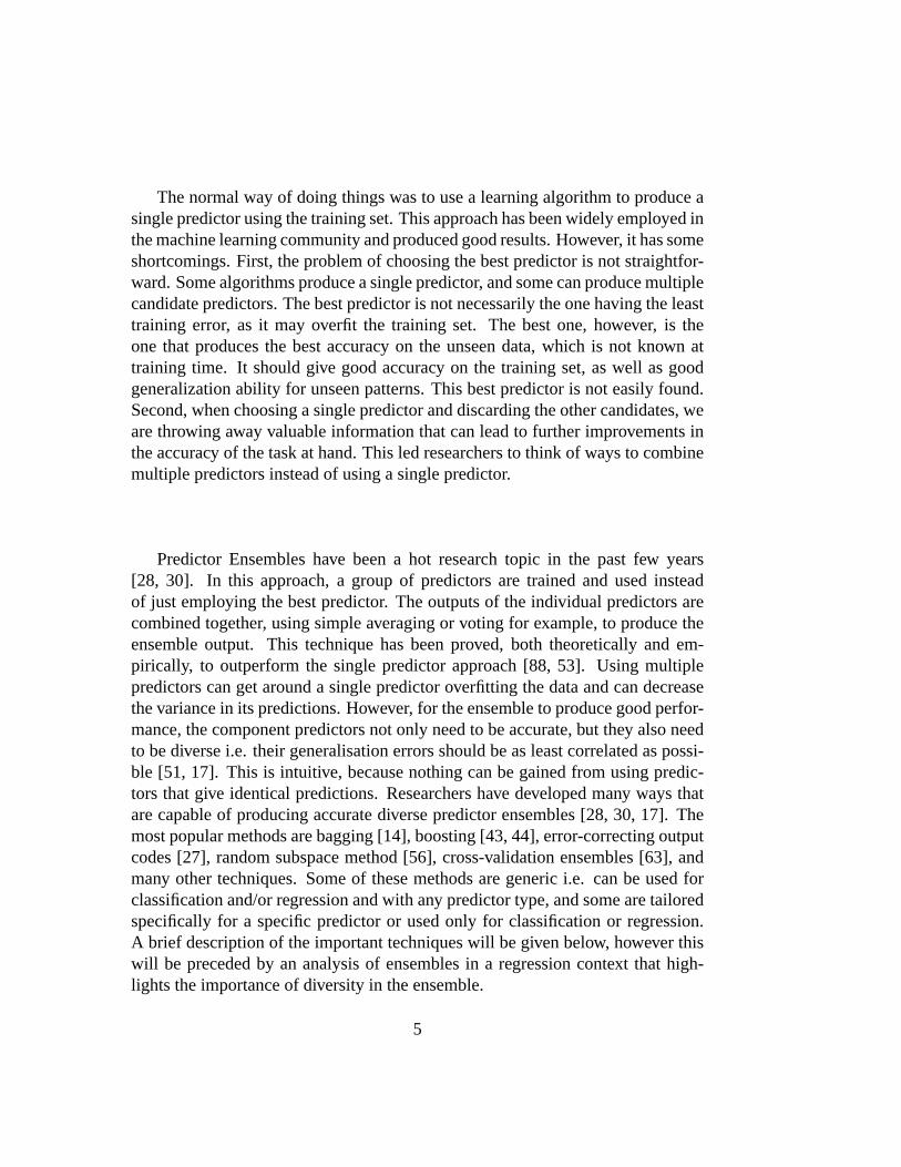
The normal way of doing things was to use a learning algorithm to produce asingle predictor using the training set. This approach has been widely employed inthe machine learning community and produced good results. However, it has someshortcomings. First, the problem of choosing the best predictor is not straightfor-ward. Some algorithms produce a single predictor, and some can produce multiplecandidate predictors. The best predictor is not necessarily the one having the leasttraining error, as it may overfit the training set. The best one, however, is theone that produces the best accuracy on the unseen data, which is not known attraining time. It should give good accuracy on the training set, as well as goodgeneralization ability for unseen patterns. This best predictor is not easily found.Second, when choosing a single predictor and discarding the other candidates, weare throwing away valuable information that can lead to further improvements inthe accuracy of the task at hand. This led researchers to think of ways to combinemultiple predictors instead of using a single predictor.
Predictor Ensembles have been a hot research topic in the past few years[28, 30]. In this approach, a group of predictors are trained and used insteadof just employing the best predictor. The outputs of the individual predictors arecombined together, using simple averaging or voting for example, to produce theensemble output. This technique has been proved, both theoretically and em-pirically, to outperform the single predictor approach [88, 53]. Using multiplepredictors can get around a single predictor overfitting the data and can decreasethe variance in its predictions. However, for the ensemble to produce good perfor-mance, the component predictors not only need to be accurate, but they also needto be diverse i.e. their generalisation errors should be as least correlated as possi-ble [51, 17]. This is intuitive, because nothing can be gained from using predic-tors that give identical predictions. Researchers have developed many ways thatare capable of producing accurate diverse predictor ensembles [28, 30, 17]. Themost popular methods are bagging [14], boosting [43, 44], error-correcting outputcodes [27], random subspace method [56], cross-validation ensembles [63], andmany other techniques. Some of these methods are generic i.e. can be used forclassification and/or regression and with any predictor type, and some are tailoredspecifically for a specific predictor or used only for classification or regression.A brief description of the important techniques will be given below, however thiswill be preceded by an analysis of ensembles in a regression context that high-lights the importance of diversity in the ensemble.
5

2.3 Diversity in Predictor Ensembles
Ensembles of identical predictors are of no use, because averaging or combiningtheir outputs does not change it. For ensembles to be better than a single predictor,the individual predictors should have uncorrelated errors regarding the test data.Krogh & Vedelsby [63] proved that, at a single data point, the square error of theensemble is guaranteed to be less than or equal to the average square error of thecomponent predictors:
(fens − d)2 =∑
i
wi(fi − d)2 −∑
i
wi(fi − fens)2, (2.1)
wherefensis the ensemble output and equals∑
i wi fi, fi is theith predictor output,wi is theith predictor weight such that
∑i wi = 1, andd is the actual value. As can
be seen in equation 2.1, the ensemble square error will be less than the individualsquare errors, only provided that they have diverse errors. The term on the right iscalled theAmbiguity Term, as it signifies the disagreement between the componentpredictors and the whole ensemble. The proof for equation 2.1 can be found in[63], but a simpler proof is also provided in [17], which is described below.
∑i
wi(fi − d)2 =∑
i
wi(fi − fens + fens − d)2
=∑
i
wi[(fi − fens)2 + (fens − d)2 + 2(fi − fens)(fens − d)]
=∑
i
wi(fi − fens)2 +
∑i
wi(fens − d)2 +
2∑
i
wi(fi − fens)(fens − d) (2.2)
=∑
i
wi(fi − fens)2 + (fens − d)2 +
2(fens − d)∑
i
wi(fi − fens) (2.3)
The rightmost term in 2.3 vanishes tozero as the sum of the weights∑
i wi =1. This leads to the result in 2.1 above. This result was quite encouraging to theensemble learning community, and it lead researchers into thinking of differentways to create diverse ensemble predictors. The next two sections describe twoof the most spread ensemble creation algorithms, namelybaggingandboosting.They both rely on the idea of sub-sampling the training set by creating a differenttraining set for each predictor, but they differ in the way this set is sampled.
6

2.4 Bagging
Bagging (an acronym forBootstrapaggregating) is one way of creating diversepredictor ensemble , and it can accomplish this through creating different trainingsets for each predictor. Bagging is based on the idea of bootstrap sampling [14]. Adifferent training set is presented to each predictor, by samplingm samples withreplacement from the original training set ofm patterns. Each sample is called abootstrap sample[38, 53], and that is where the algorithm got its name from. Bysampling with replacement, some patterns will be repeated more than once, otherswill be absent, however, on the average, 63.2% of the original training set will berepresented. After training all the individual predictors, the final ensemble outputis the simple average of the component predictors outputs. Algorithm 1 describesthe bagging procedure.
Algorithm 1 BAGGING
Inputs:a setS of m training patterns:S ={(xi,yi), i = 1, . . . ,m}, wherexi is theithvector of features andyi is theithtarget value,LEARN: a learning algorithm ,K: the number of predictors to return,
Outputs:an ensembleE of K predictors:E = {Ck, k = 1, . . . , K}
Procedure:1: for k = 1 : K do2: createTk {a bootstrap training set of sizem}3: Ck :=LEARN(Tk) {train the predictor}4: end for
Bagging has been shown to perform better than single predictors [14, 86, 67,99, 7, 29, 79, 88, 50]. It was also shown that it can perform better than otherensemble learning techniques, specially in noisy environments. The only require-ment for bagging to produce good diverse ensembles is the instability of the train-ing algorithm [14]. As long as the bootstrap sampling from the original trainingcauses the training algorithm to produce nonidentical predictors, then bagging isguaranteed, on the average, to produce better results.
The main advantage of bagging is its simplicity in application and its paral-lelizability. The individual predictors are independent of each other, and so they
7
can be created simultaneously. In addition, it is applicable to both classificationand regression, and does not need any change in the base learning algorithm. Inthe case of classification, simple majority voting can be used, and in case of re-gression a simple average of the outputs is employed.
2.5 Boosting
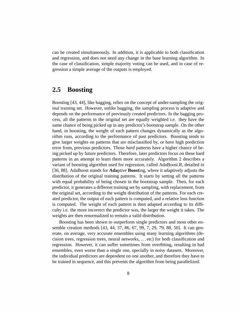
Boosting [43, 44], like bagging, relies on the concept of under-sampling the orig-inal training set. However, unlike bagging, the sampling process is adaptive anddepends on the performance of previously created predictors. In the bagging pro-cess, all the patterns in the original set are equally weighted i.e. they have thesame chance of being picked up in any predictor’s bootstrap sample. On the otherhand, in boosting, the weight of each pattern changes dynamically as the algo-rithm runs, according to the performance of past predictors. Boosting tends togive larger weights on patterns that are misclassified by, or have high predictionerror from, previous predictors. Thosehard patterns have a higher chance of be-ing picked up by future predictors. Therefore, later predictors focus on these hardpatterns in an attempt to learn them more accurately. Algorithm 2 describes avariant of boosting algorithm used for regression, called AdaBoost.R, detailed in[36, 88]. AdaBoost stands forAdaptive Boosting, where it adaptively adjusts thedistribution of the original training patterns. It starts by setting all the patternswith equal probability of being chosen in the bootstrap sample. Then, for eachpredictor, it generates a different training set by sampling, with replacement, fromthe original set, according to the weight distribution of the patterns. For each cre-ated predictor, the output of each pattern is computed, and a relative loss functionis computed. The weight of each pattern is then adapted according to its diffi-culty i.e. the more incorrect the predictor was, the larger the weight it takes. Theweights are then renormalized to remain a valid distribution.
Boosting has been shown to outperform single predictors and most other en-semble creation methods [43, 44, 37, 86, 67, 99, 7, 29, 79, 88, 50]. It can gen-erate, on average, very accurate ensembles using many learning algorithms (de-cision trees, regression trees, neural networks, . . . etc) for both classification andregression. However, it can suffer sometimes from overfitting, resulting in badensembles, even worse than a single one, specially in noisy datasets. Moreover,the individual predictors are dependent on one another, and therefore they have tobe trained in sequence, and this prevents the algorithm from being parallelized.
8

Algorithm 2 ADABOOST.RInputs:
a setS of m training patterns:S ={(xi,yi), i = 1, . . . ,m}, wherexi is theithvector of features andyiis theithtarget value,LEARN: a learning algorithm ,K: the number of predictors to return
Outputs:an ensembleE of K predictors:E = {Ck, k = 1, . . . , K}
Initialize:w
(1)i := 1/
∑mi=1 wi {initialize weights of training set}
Procedure:for k := 1, . . . , K do {loop on number of predictors}
construct a training setTk using the distributionw(k)
Ck :=LEARN(Tk) {train predictorCk using bootstrap sampleTk}y
(k)i := Ck(xi) for all i, i = 1, . . . ,m
Li :=|yi
(k)−yi|D
for all i, whereD := maxi=1...m |yi(k) − yi| {loss for each
pattern}L : =
∑mi=1 Liw
(k)i {average loss function}
βk := L1−L
{confidence measure}
w(k+1)i := w
(k)i β
(1−Li)k
w(k+1)i :=
w(k+1)i∑
iw
(k+1)i
{normalize weight so that it remains a distribu-
tion}end for
9

2.6 Other Ensemble Creating Techniques
Many more ensemble creating algorithms have been investigated by researchers,however the most two important are bagging and boosting. Bagging and boostingtry to create diverse ensembles by manipulating the distribution of the training setpresented to each individual predictor. Other techniques try to achieve the sameobjective by manipulating the output class labels [27], the input features [56],or by using algorithm-specific property that injects randomness into the differentpredictors [82, 99, 29]. As indicated, some of these techniques are applied tospecific algorithms and can not be used by any general learning algorithm, someare used only for classification and can not be used for regression, and some aregeneral to be used with any algorithm or application.
2.7 Summary
Ensemble learning employs a committee of predictors for solving the problem athand instead of just using one predictor. A group of predictors was proved to bebetter than single predictors for many practical problems. For the ensemble to beaccurate, the individual predictors need to be both accurate and different. Manyways are used to create accurate diverse ensembles, the two major of which arebagging and boosting.
10

Chapter 3
Feature Subset Selection
3.1 Introduction
Feature selection is a very important part of the preprocessing phase in machinelearning [59, 28, 61] and statistical pattern recognition [102, 58, 53, 66]. In manyreal world situations, we are faced with problems having hundreds or thousandsof features, some of which are irrelevant to the problem at hand. Feeding learningalgorithms with all the features can result in a deteriorating performance, as thealgorithm can get stuck trying to figure out which features are useful and whichare not. Therefore, feature selection is employed as a preliminary step, to selecteda subset of the input features, that contains potentially more useful features. Inaddition, feature selection tends to reduce the dimensionality of the feature space,avoiding the well-known dimensionality curse problem [53].
Feature selection is a non-trivial procedure, as the search space grows expo-nentially with the number of features e.g. forn features there are2ndifferentsubsets that should be examined and evaluated. Many different techniques havebeen proposed to solve this difficult problem. An overview of the feature selectionprocess is given below, followed by a description of sequential feature selectiontechniques that are used in this work. They are among the most robust and stablefeature selection algorithms.
3.2 Feature Selection Process
Feature selection consists of the four major steps [66] in figure 3.1. Subset gen-eration is a search procedure through the feature space that produces candidate
11
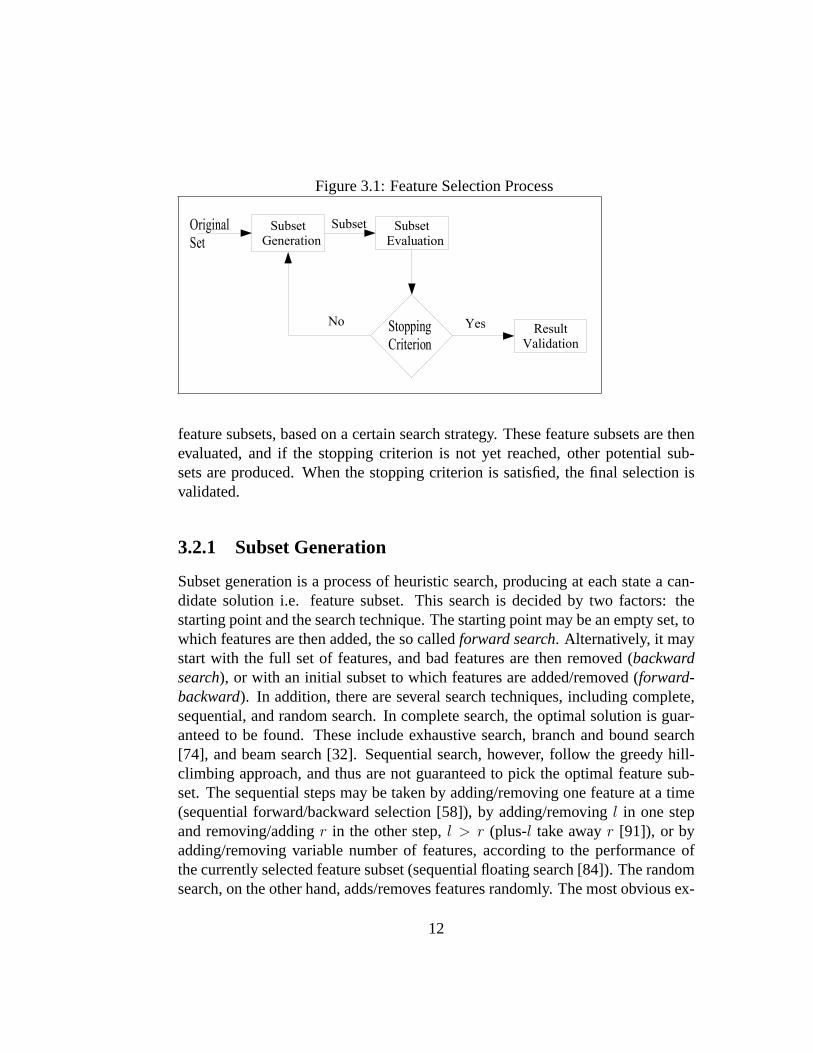
Figure 3.1: Feature Selection Process
Subset Generation
Subset Evaluation
ResultValidation
OriginalSet
No Yes
Subset
StoppingCriterion
feature subsets, based on a certain search strategy. These feature subsets are thenevaluated, and if the stopping criterion is not yet reached, other potential sub-sets are produced. When the stopping criterion is satisfied, the final selection isvalidated.
3.2.1 Subset Generation
Subset generation is a process of heuristic search, producing at each state a can-didate solution i.e. feature subset. This search is decided by two factors: thestarting point and the search technique. The starting point may be an empty set, towhich features are then added, the so calledforward search. Alternatively, it maystart with the full set of features, and bad features are then removed (backwardsearch), or with an initial subset to which features are added/removed (forward-backward). In addition, there are several search techniques, including complete,sequential, and random search. In complete search, the optimal solution is guar-anteed to be found. These include exhaustive search, branch and bound search[74], and beam search [32]. Sequential search, however, follow the greedy hill-climbing approach, and thus are not guaranteed to pick the optimal feature sub-set. The sequential steps may be taken by adding/removing one feature at a time(sequential forward/backward selection [58]), by adding/removingl in one stepand removing/addingr in the other step,l > r (plus-l take awayr [91]), or byadding/removing variable number of features, according to the performance ofthe currently selected feature subset (sequential floating search [84]). The randomsearch, on the other hand, adds/removes features randomly. The most obvious ex-
12

amples for random search are Genetic Algorithm approaches for feature selection[89, 47, 76].
3.2.2 Subset Evaluation
After generating candidate feature subsets, they have to be evaluated to select thebest solution. There are two approaches for feature subset evaluation: the filterand the wrapper models [61]. In the filter model, each feature subset is evaluatedbased on the intrinsic data between the features, independently of the learningalgorithm. The wrapper model, on the other hand, employs the learning algorithmas a black box in the evaluation process. The feature subset is evaluated based onits performance, using the learning algorithm, on a validation set, or usingk-foldcross-validation [59, 60] on the training set. Ink-fold cross-validation, the trainingset is partitioned intok equal subsets, and the learning algorithm is evaluatedkindependent times. In each time, one of thek subsets is used for testing, whileusing the otherk− 1 subsets for training. The final evaluation is an average of thek runs. The wrapper model is more computationally expensive than the featuremodel, however it usually gives better results.
3.2.3 Stopping Criteria
The stopping criteria are checked after each candidate subset is generated andevaluated, and the search procedure stops when they are satisfied. The criteriamay include: the end of the search process, some limit on the feature subset size,the number of iterations is reached, or deterioration of performance on the addi-tion/deletion of any further feature to the subset.
3.2.4 Result Validation
The best selected feature subset from the above steps has to be validated. Thevalidation can use prior knowledge about the problem, in case it is available. Oth-erwise, the performance of the selected set can be evaluated using the presenttraining set, or a separate validation set, or again usingk-fold cross-validation.
13

3.3 Sequential Feature Selection Algorithms
As described above, many techniques have been used for efficient feature selec-tion. Sequential feature selection, though considered sub-optimal, is among themost robust and widespread feature selection algorithms [59]. Two versions ofsequential feature selection will be described here: Sequential Forward Selection(SFS) and Sequential Floating Forward Selection (SFFS). The subset evaluationfollows the wrapper approach, in whichk-fold cross-validation is used to estimatethe feature subset performance. The training set is divided up intok equal parts.The training operation is performedk times, where each part is used once as atest set while training using the otherk − 1 parts. The final error estimation is theaverage of thek error estimates computed [60]. The stopping criteria employedis the deterioration of the subset performance i.e. the algorithm stops when theaddition of new features results in a reduced performance.
3.3.1 Sequential Forward Selection
SFSis considered among the simplest approaches for feature selection. It startswith an empty feature set, and adds one feature at a time. The feature added isthe one that optimizes the objective function value of the currently selected subsetincluding the newly added feature. Addition of new features continues until nofurther improvement in performance can be achieved. Performance is measuredusing 10-fold cross-validation on the training set. Algorithm 3 outlines theSFS.
3.3.2 Sequential Floating Forward Selection
Pudil et al. [84] introduced a modification on theSFSalgorithm, called the float-ing search methods. The difference added to theSFSis a backward eliminationstep after the addition of each new feature. Here, the forward addition is uncon-ditional i.e. the best new feature is added to the current subset regardless of thenew subset performance. However, the backward elimination step continues toremove features from the subset as long as this improves the performance. It wasshown thatSFFSperforms very well, compared to other sequential algorithms[58]. Algorithm 4 outlines theSFFS.
14

Algorithm 3 Sequential Forward SelectionInput:
S = {(xi, yi), i = 1, . . . ,m} {training set of m patterns andk fea-tures}A {a learning algorithm}
Output:Jbest = {j, j ∈ {1, . . . , k}} {the best feature subset}
Procedure:Jbest := φ {initialize to empty set}ηbest := eval(Jbest, S, A) {evaluate the subset using 10-fold cross-validationusing the algorithmA and the training setS}while (true) do
for k = 1, . . . , K do {for all the features}J := Jbest + k {add the feature to the subset}ηk := eval(J, S,A) {evaluate its performance}
end for(η, k) := maxk ηk {get the feature that achieves maximum perfor-mance}if η > ηbest then {if the best feature improves the performance}
Jbest := Jbest + k {add it to the subset}ηbest = η {updateηbest}
elsereturnJbest {exit and return the best subset feature}
end ifend while
15

Algorithm 4 Sequential Floating Forward SelectionInput:
S = {(xi, yi), i = 1, . . . ,m} {training set of m patterns andk fea-tures}A {a learning algorithm}
Output:Jbest = {j, j ∈ {1, . . . , k}} {the best feature subset}
Procedure:Jbest := φ {initialize to empty set}ηbestf := eval(Jbest, S, A) {evaluate the subset using 10-fold cross-validationusing the algorithmA and the training setS}while (true) do
{Step 1: unconditional forward selection step}for k = 1, . . . , K do {for all the features}
J := Jbest + k {add the feature to the subset}ηk := eval(J, S,A) {evaluate its performance}
end for(ηf , kbest) := maxk ηk {get the feature that achieves maximum perfor-mance}Jbest := Jbest + kbest {add the best feature to the subset}ηbestb = ηf {bestη in the backward step that follows}ηbestf = ηf {save the current performance}while ηbestb ≥ ηf do
{Step 2: the conditional backward elimination step}for k = 1, . . . , length(Jbest) do
J := Jbest − k {remove feature from the subset}ηk := eval(J, S,A) {evaluate the new subset}
end for(η, kbest) := maxk ηk {get the feature that achieves maximum perfor-mance}if η > ηbestb then
Jbest := Jbest − kbest {remove the worst feature}ηbestb = η {updateηbestb}
end ifend while{check if the last step deteriorated the performance}if ηbestb < ηbestf then
undo the last additionreturnJbest
end ifend while
16

3.4 Summary
Feature selection is considered an important preprocessing step in machine learn-ing problems. It tries to focus the attention of the learning algorithm on a smallsubset of features of potential importance to the problem at hand. Numerous ap-proaches have been used to get this small useful feature subset, of which sequen-tial feature selection techniques are among the most stable.
17

Chapter 4
Literature Survey
4.1 Introduction
Ensemble learning is a powerful tool in the field of machine learning. For a predic-tor ensemble to produce better performance, the constituent predictors have to beaccurate and diverse. Many directions have been investigated in order to achievediverse accurate ensembles. The approach focused on here is the manipulationof input features to the individual predictors. The idea of partitioning the inputfeatures among individual predictors arises from the idea of feature selection. Infeature selection problems, there exists a large number of features available thatcan not all be used in the learning process. Some way of choosing the most repre-sentative subset of these features must be employed. The disadvantage of featuresubset selection is that some features that may seem less important, and are thusdiscarded, may bear valuable information.
This is where Feature Subset Ensemble (FSE) comes into play. It simply par-titions the input features among the individual predictors in the ensemble. Hence,no information is discarded. It serves at uitilizing all the available information inthe training set, and at the same time not overloading a single predictor with allthe features, as this may lead to poor learning.
Some attempts have been made to find a systematic way of distributing theinput features among the different predictors. These techniques used random se-lection [55, 8, 56, 18], traditional feature selection algorithms [4, 49], genetic al-gorithm approach [78, 48, 77], manual selection of features [23], grouping basedon the correlation properties between features [65, 93, 80], and algorithm-specificfeature manipulation [99, 29, 16]. Most of these methods achieved encouraging
18
results and proved useful in the sample datasets they were applied to. These di-rections will be discussed in detail below.
4.2 Random Feature Subset Selection Approach
Ho [55, 56] proposed a technique calledRandom Subspace Method (RSM). Inthis technique, a subset of features was randomly selected for each predictor. Sheused C4.5 decision trees [85] as the base predictor. The number of features se-lected for each predictor was half the total number of features. Experiments wereundertaken to compare the RSM to bagging, boosting and single tree predictorsemploying all features. Four publicly available datasets from Project StatLog [12]were used. In each ensemble technique, a decision forest was grown up to100decision trees. RSM showed better performance than bagging, boosting, and sin-gle tree predictor. In addition, further experiments were conducted to assess theeffect of the feature subset size on the ensemble performance. She pointed out thatusing half the number of features produced acceptable results. The technique canbe used with any training algorithm other than decision trees, and can be appliedto either regression or classification. However, the feature subset size should notbe limited to half the number of features, as this depends on the correlation andredundancy between features.
Bay [8] introduced a similar idea, calledMultiple Feature Subsets (MFS). Inthis method, he applied random feature selection to nearest neighbor (NN) pre-dictors. Each NN predictor was trained using a random subset of features. Baynoticed that other ensemble learning techniques, e.g. bagging or boosting, thatdepend on subsampling the training set, failed to improve NN ensembles. There-fore, he worked on another method that manipulated input features instead ofinput patterns. Bay used two sampling functions: sampling with replacement andsampling without replacement. In sampling with replacement, a given feature canbe replicated within the same predictor. In sampling without replacement, how-ever, a given feature can not be assigned more than once to the same predictor.Each of the NN predictors used the same number of randomly selected features.The algorithm has two parameters, the feature subset size, and the ensemble size.The latter was fixed to 100 predictors, and the former is chosen using 10-foldcross-validation on the training set using 10 evenly spaced values. Bay devel-oped two versions of his approach: MFS1 (using sampling with replacement) andMFS2 (using sampling without replacement). The output of the predictors werecombined using simple voting. These two versions were compared to four other
19

algorithms: nearest neighbor (NN),k nearest neighbor (kNN), nearest neighborwith forward (FSS), and backward (BSS) sequential selection [102]. The value ofk in kNN was computed using 10-fold cross-validation on the training data. Thefeature selection used cross-validation for accuracy estimation, which is knownas the wrapper approach [59, 61]. Bay used 25 publicly available classificationdatasets from UCI repository [10] to evaluate the compared algorithms. Bay tookthe average of 30 independent runs for each algorithm, in each one2
3of the pat-
terns were selected as the training set and the remaining used as the test set. Bayreported that the two versions of his approach, MFS1 and MFS2, performed betterthan the other algorithms in all but two datasets. Bay’s approach was applied toclassification only, nevertheless it can be applied to both classification and regres-sion. In fact, it is the same idea of Random Subspace Method, but applied to adifferent predictor type.
Bryll et al. [18] also used a similar approach, which they calledAttributeBagging (AB). In this approach, each predictor is trained on a subset of randomlyselected features (without replacement). They proposed a framework, in whichthe size of the feature subset is determined first, and this parameter is problemdependent. Then, various subsets of that size are evaluated using the wrappermethod [61], and only the best of these subsets are used for voting. Bryll et al.evaluated their method on a hand-pose recognition dataset [97] using OC1 deci-sion tree algorithm [72]. The dataset consists of 29 attributes, 20 classes, 934training patterns, and 908 testing patterns. They tested different subset sizes andfound that using1
3of the attributes with an ensemble of 25 predictors gave the
best results. They tried both unweighted and weighted voting of the individualpredictors, where the weights were proportional to their accuracy on the train-ing set. The results reported were the average of 30 independent runs. Bryll etal. compared their approach to single OC1 trees, bagged OC1 ensembles, ID3,RIEVL and others. Their algorithm showed better results than all of these algo-rithms. AB is a generic approach that can be used with any learning algorithm,and for both classification and regression. However, it is not flexible enough, asits parameters, the attribute subset size and the ensemble size, are hand selectedand are not computed automatically from the training set.
The methods discussed above are nearly similar in that they assign featuresrandomly to each individual predictor. They differ in the way their parameters(subset and ensemble sizes) are estimated. In addition, they were tested only onclassification problems not regression tasks.
20

4.3 Traditional Feature Subset Selection Approach
Alkoot and Kittler [4] proposed an approach that uses traditional feature selec-tion algorithms in order to maximize the overall ensemble performance. Theyproposed three different variations for building the ensemble: the parallel system,the serial system, and the optimized conventional system. In the parallel system,eachexpert(the term they used for apredictor) is allowed, in turn, to take onefeature such that the overall ensemble performance is optimised on a validationset. In the serial system, in contrast, the first expert is allowed to take all the fea-tures that achieve the maximum ensemble accuracy on the validation set. If somefeatures remain, a second expert is used, and so on. The optimized conventionalsystem builds each expert independently, and then features are added/deleted fromthe ensemble as long as the ensemble performance is increased. Three differentpredictor algorithms were used: gaussian,k Nearest Neighbor (kNN), and Near-est Neighbor (NN). Two classification datasets were employed: Breast CancerWisconsin [10] from UCI repository, and Seismic from the University of Surrey.These approaches were compared only to single predictor, and no comparison toother ensemble learning techniques was carried out. Alkoot and Kittler reportedthat their algorithm performed, on the average, better than single predictor ap-proach.
Günter and Bunke [49] proposed an ensemble creation technique based onfeature selection algorithms. They tested their method in the context of handwrit-ten word recognition, using Hidden Markov Model (HMM) recognizer [69] as thebase predictor. In their approach, each predictor is given a well performing set offeatures using any existing feature selection algorithm. The only modification thatmust be made to the feature selection algorithm is to prevent identical feature sub-sets from being returned. Therefore, the feature selection algorithm tries to get thebest unrepeated feature subset with respect to a given objective, and given a list ofpreviously generated feature subsets. Günter and Bunke used two well known al-gorithms: floating sequential forward and backward search algorithms [84]. Eachpredictor uses one of the two floating search algorithms to get a unique featuresubset. Two objective functions were experimented: the recognition performanceon the validation set, and another one that combines a measure of the ensemblediversity with the above accuracy. Günter and Bunke compared their approach tofloating forward search, floating backward search, and random subspace method[56] using50% of the features. The ensemble size employed was 10 predictors.They reported that their approach outperformed the other techniques on the useddataset. This approach is generic, and can be used with any feature selection algo-
21

rithm other than the floating search algorithm, and on regression or classificationtasks. However, it was not compared to other ensemble creating techniques suchas bagging or boosting.
4.4 Genetic Algorithm Approach
Opitz [78] presented a Genetic Algorithm (GA) approach for ensemble creation,called Genetic Ensemble Feature Selection (GEFS). Opitz noted that GA can beused to search through the large space of feature subsets, and to select the best ofsuch subsets to create a powerful predictor ensemble, such that those subsets cre-ate a diverse ensemble. He argued that this task is an enormous problem, and canbe tackled using global optimization techniques such asGAs. In this technique, astartup population of Artificial Neural Networks (ANNs) is initially trained usingrandomly selected feature subsets (with replacement) with random subset sizes.Then, theGA is run on this population, using the genetic operators of mutationand cross-over, producing more fit children in each new population according to afitness function. The fitness function employed combines the individual network’saccuracy with its disagreement (diversity) with the entire ensemble. Experimentswere performed using 21 classification datasets from the University of WisconsinMachine Learning Repository and the UCI data set repository [10]. The results re-ported are the average of five independent iterations using standard 10-fold cross-validation on the datasets. For each fold an ensemble of 20 networks is created, fora total of 200 networks per dataset, each trained using standard back-propagationlearning algorithm. Opitz compared his approach to single network, bagging, andboosting (AdaBoost). The results reported that it compared favorably to baggingand boosting, as it outperformed bagging in 15 datasets, tied in 6; and outper-formed boosting in 16, tied in 4, and lost in 1. Obviously, the algorithm is genericand can be used with any predictor type other than Artificial Neural Networks,and also for regression or classification.
Guerra-Salcedo and Whitley [48] proposed anotherGA-based approach forensemble creation. However, they used table-based predictors, namely KMA [31]and Euclidean Decision Tables (EDT)[47]. They applied the CHC genetic searchalgorithm [39]. Experiments were carried out using three classification datasetsfrom Project StatLog [12] and UCI repository [10]. The datasets were called Seg-ment, LandSat, and DNA and had 19, 36, and 180 features respectively. In theirexperiments, they compared different combinations of ensemble building tech-niques with feature selection techniques. For ensemble building, they used all the
22
training set, bagging, and two versions of boosting. For feature subset selectionfor each predictor, they applied CHC genetic search, Random Subspace Method[56], and all available features. The results reported were the average of 10 inde-pendent runs over the 3 datasets. In each run, CHC was operated 50 times using50 different random splits of the training set into training and validation sets, andgenerated 50 good feature subsets. The fitness function employed used only theaccuracy of the individual predictors on the validation set, yet it did not considerany diversity measure inside the ensemble. The 50 generated feature subset weredistributed over 50 predictors. Guerra-Salcedo and Whitley reported that theirapproach exhibited encouraging results and outperformed, on the average, therandom subspace method and using all the features.
Oliveira et al. [77] also proposed aGA-based ensemble creation technique.Their technique also used aGA to find good feature subsets, however they em-ployed a hierarchical two-phase approach to ensemble creation. In the first phase,a set of good predictors are generated using Multi-Objective Genetic Algorithm(MOGA) search[76]. The base predictors used were Artificial Neural Networks(ANN), however any type of predictor can be used. The second phase searchesthrough the space created by the different combinations of these good predictors,again usingMOGA, to find the best possible combination i.e. the best ensemble.The objective function in the first phase was the accuracy of theANN measuredusing sensitivity analysis [71]. In the second phase, two objective functions wereused: one measuring the generalization error of the ensemble, and the other mea-suring its ambiguity [63]. The method was experimented in the context of hand-written digit recognition, using NIST SD19 database. Oliveira et al. comparedtheir method to singleANNpredictors, using three different feature sets. They re-ported that their method outperformed the singleANNand used about 5 predictorsin the ensemble, however no comparison to other ensemble creating method wascarried out.
4.5 Manual Feature Subset Selection Approach
Cherkauer [23] introduced a system called PLANNETT (Person-Level ArtificialNeural Networks for ExtraTerrestrial Terrain classification), which combines ANNsin order to achieve better accuracy in the difficult task of recognizing volcanoesin radar images of planet Venus. Experiments were carried out using four imagesfrom the Magellan space probe containing together 163 volcanoes that are labeledby human experts [90]. A total set of 119 features are extracted from each part of
23
the image that contain a potential volcano. These 119 features were divided into8 hand-selected feature subsets, each one given four ANNs. The ANNs given thesame subset differ in the number of hidden nodes, having either 0, 5, 10, or 20hidden nodes. The 32 networks are trained using standard backpropagation. Thefinal output of the ensemble is the simple average of the 32 ANNs. The PLAN -NETT system replaces the existing classification module in the JARTOOL systemdeveloped at NASA’s Jet Propulsion Laboratory [19]. Cherkauer reported that hisnew classification module, PLANNETT, outperformed the old one, achieving theaccuracy of a human planetary geologist. This method is problem-specific andcan not be applied systematically to any other dataset.
4.6 Correlation-Based Feature Subset Selection Ap-proach
Liao and Moody [65] proposed a technique calledInput Feature Grouping. Thefirst step in the technique is to group the input features into clusters based on theirmutual information, such that features in each group are greatly correlated to eachother, and are as little correlated with features in other groups as possible. In thesecond step, each member of the ensemble is given a representative of each fea-ture cluster. Liao and Moody applied their technique on an economic forecastingproblem having 9 input features. A hierarchical clustering algorithm [40] wasused to cluster the input features. The inputs were divided into four groups. Eigh-teen different ANNs were constructed, each given one feature from each of thefour groups. They compared their method with three other ensemble techniques:baseline, random selection, and bagging. In the baseline method they trained thenetworks using all the features, and they only differed in their initial weights.Twenty independent runs were performed for each of the four methods. Liao andMoody reported that their approach outperformed the other three methods.
Tumer and Oza [93, 80] presented an approach calledInput Decimation En-sembles (IDE). Their method is only applicable to classification tasks. For a clas-sification problem withL class labels, it constructsL predictors. Each predictoris given a subset of the input features, such that these features are the most cor-related with that class. The ensemble final output is the average of the individualpredictors output. They compared their method to a single predictor with all inputfeatures, and to Principal Component Analysis (PCA) ensembles [53], a well-known dimensionality reduction technique. They employed three real world [93]
24
and three synthetic [80] datasets. Artificial Neural Networks were used as the basepredictors, trained using standard backpropagation. Tumer and Oza reported thattheir method outperformed the single predictor and thePCAensemble, speciallyin datasets with large number of input features. However, they did not comparetheir method to other standard ensemble techniques.
4.7 Algorithm-Specific Feature Manipulation
Zheng and Webb [99] introduced an approach specific to the decision trees, spe-cially C4.5 [85] decision trees, and called itStochastic Attribute Selection Com-mittee (SASC). The key idea is to create diverse predictors by manipulating theattributes available at each decision in the tree. For each node, a subset of the at-tributes (features) is stochastically selected, and that node is restricted to make itsdecision from these attributes. They carried out experiments on 40 natural domainclassification datasets from UCI repository [10], and compared their approach tosingle C4.5 trees, bagging, and boosting. Two stratified 10-fold cross-validationswere run for each algorithm, and the average of the 20 runs were recorded. Zhengand Webb reported that SASC outperformed the single tree and bagging, on aver-age. Nevertheless, boosting was superior to both SASC and bagging. They arguethat their method, like bagging, is amenable to being parallelized, unlike boostingin which each tree depends on previous ones. In addition, bagging and SASCare more stable than boosting. Zheng and Webb investigated the idea further, bycombining SASC with bagging to form SASCBAG [98], combining SASC withboosting to form SASCB [101], or combining both bagging and boosting withSASC to form SASCMB [100]. All these methods were applied to C4.5 decisiontrees, and required modification to the base tree induction algorithm.
Dietterich [29] proposes a related approach to generate diverse C4.5 decisionforests. The method, at each internal node in the tree, identifies the best 20 pos-sible splits, and chooses one at random. Experiments were undergone on 33 clas-sification datasets from UCI repository [10]. The randomized C4.5 trees werecompared to single C4.5 trees, bagging, and boosting. He used ensembles of 200trees for both randomized C4.5 and bagging, and 100 for boosting. The threeensemble techniques outperformed, as expected, the single tree. Bagging and ran-domized C4.5 gave quite similar results, while boosting was superior in most ofthe datasets.
Breiman [16] presented an approach quite near to SASC, calledRandom Forests.In this approach, bagging is combined with random feature selection. Each tree
25

in the ensemble is trained using a different bootstrap sample of the training set,and the remaining out-of-bag patterns are used as a validation set. There are twoversions of the method regarding the random feature selection at each node. Thefirst, calledForest-RI, selects a random subset of features to split on. The sec-ond version,Forest-RC, takes a random combination of randomly selected inputs,and makes the split on these generated features. The base tree predictor used wasCART[13]. For classification, Breiman compared his method to a single tree, andAdaBoost using 20 classification datasets. For regression, Random Forests werecompared to bagging and adaptive bagging [15] using 8 regression datasets. Hereported that his method compared favorably to AdaBoost (in classification) andto adaptive bagging (in regression).
4.8 Summary
We investigated several techniques for creating diverse ensembles, which all reliedon manipulating input features. All, except two, of these techniques were imple-mented and tested on classification tasks, with some of them applicable only toclassification. Some of them were algorithm-specific i.e. can be used only withcertain type of learning algorithm. They were all reported to outperform singlepredictor, and other ensemble techniques, including bagging and boosting, spe-cially in datasets with many input features. This is due to the fact that featuredistribution among predictors tends to reduce the dimensionality of the problem.
Table 4.1 presents a summary of the techniques discussed. They are groupedinto categories according to the techniques used for distributing the features amongpredictors in the ensemble. The employed learning algorithm is listed for eachtechnique, together with the kind of task experimented,C for Classification andR for Regression. The applicability of the technique is denoted in the column la-beledGeneric, with yesfor completely generic techniques that can be used withany learning algorithm for either classfication or regression.
26

Table 4.1: Summary of Feature Distribution Techniques
Category Method Learning Algorithm Task Generic
Random FeatureSelection
RSM [56] C4.5 trees C yesMFS [8] NN C yesAB [18] OC1 trees C yes
Traditional FeatureSelection
[4] NN, kNN and Guassian C yes[49] HMM C yes
GA Feature SelectionGEFS [78] ANN C yes[47] KMA and EDT C yes[77] ANN C yes
Manual FS PLANNETT [23] ANN C yesCorrelation FeatureSelection
IFG [65] ANN R yesIDE [93, 80] ANN C C only
Algorithm-Specific FSSASC, SASCBAG,SASCB, andSASCMB[99, 98, 101, 100]
C4.5 trees C C4.5 only
Randomized C4.5[29]
C4.5 trees C C4.5 only
Random Forests[16]
CART C & R CART only
27

Chapter 5
FSE Comparison and Variants
5.1 Introduction
We adopted two approaches in this work. The first is to compare basic FeatureSubset Ensembles (FSE) based on random subset selection of features to threetypes of single-predictor systems and two well known ensemble systems. Thiscomparison focused on regression datasets. The comparison also tried to figureout the effect of training set size on the accuracy of these techniques. Secondly, wetried to introduce some variants to the basic random subset selection algorithm,in an attempt to increase its accuracy and reliability. These included changingthe predictors weights, using bagging, boosting, and forward selection algorithmsfrom within the random feature selection. Then, we tried to investigate other sys-tematic feature partitioning techniqus, in addition to the random feature selection.These included techniques based on feature correlation or on feature relevance.
5.2 Datasets
Our focus was on regression tasks, so we used six different regression datasets.Three of them were synthetic, and three were real-world datasets. Table 5.1 givesa summary of the datasets, showing the number of features and number of avail-able examples for each. The datasets were chosen such that they have a substantialnumber of features, in addition to a large number of patterns. This aids in perform-ing tests that can be near ground truth. The datasets are:
• bank32nh: a dataset from the Delve repository [1] synthetically generated
28

Table 5.1: Dataset Summary. Type ’S’ refers to synthetic datasets, and ’R’ refersto real-world datasets.
Dataset No. of Features No. of Patterns Type
bank32nh 32 8,192 Sailerons 40 13,750 S
syn 80 10,000 Shouse16h 16 22,784 R
comp 21 8,192 Rpole 48 15,000 R
from a simulation of how bank-customers choose their banks. Tasks arebased on predicting the fraction of bank customers who leave the bank be-cause of full queues. It consists of 8192 patterns and 32 features.
• ailerons: a synthetic dataset from the Weka Project [95]. This data setaddresses a control problem, namely flying an F16 aircraft. The attributesdescribe the status of the aeroplane, while the goal is to predict the controlaction on the ailerons of the aircraft. It consists of 40 features and 13750patterns.
• syn: a synthetically generated dataset. It consists of 80 features and 10,000patterns. The dataset is generated such that it contains 40 irrelevant features(with zero weights in the final target) and 40 relevant features (with weightschosen from a unifrom distributionU ∼ (−1, 1)). The features are alsodrawn from a multivariate normal distribution such that there is some corre-lation among the features. A noise term is added to the target, drawn froma normal distributionN ∼ (0, 1). The target output is a linear combinationof the inputs and the weights, in addition to the noise term.
• house16h:a real-world dataset from the Delve repository [1]. It predictsmedian house prices from the 1990 US census data. It consists of 22,784patterns and 16 features.
• comp: a natural domain dataset from the Delve repository [1]. It predicts acomputer system activity from system performance measures. It consists of8,192 patterns and 21 features.
29
• pole: a natural domain dataset from the Weka Project [95]. The data de-scribes a telecommunication problem. It consists of 15,000 patterns and 48features.
5.3 Comparison
In an attempt to better realize the usefulness ofFSE, we performed extensive ex-periments to assess their performance on six different regression datasets. Thealgorithm used was similar to Ho’s Random Subspace Method (RSM) [56], whichis also quite similar to Attribute Bagging (AB) [18] and Multiple Feature Subsets(MFS) [8]. Algorithm 5 describes the basic Feature Subset Ensembles (FSE) al-gorithm, the version used in this work. In this algorithm, the number of predictorsin the ensemble as well as the number of features per predictor are given as inputs.The sampling function to be used, i.e. sampling with or without replacement, isalso specified to the algorithm. The final ensemble output is the simple avarage ofthe individual predictors outputs, i.e. they all have equal weights. This algorithmwas compared to five different other algorihtms, three single-predictor and twoensemble techniques. It was compared to: a single predictor using all the features,a single predictor using Sequential Forward Selection (SFS) (algorithm 3), a sin-gle predictor using Sequential Floating Forward Selection (SFFS) (algorithm 4),bagging ensembles using all features (algorithm 1), and boosting (ADABOOST.R)ensembles with all features (algorithm 2).
All these algorithms are generic, in the sense that they can be used with anypredictor type. Therefore, to gain further insight into their operation in regressiontasks, we used three different predictor types; one linear and two non-linear. Thelinear is the famous Least Square Error predictor (LSE) [70]. The other two non-linear predictors are Artificial Neural Networks (ANN) [53] andCARTRegressionTrees [13].
5.4 FSE Variations
We tried out several variations on the basicFSEtrying to add more accuracy andstability. First, we tried two sampling functions: with and without replacement.Second, we tried to change the weighting scheme, to give higher emphasis on themore accurate predictors. Two weighting schemes were added beside the nor-mal equal weighting: weight according to training error and weight according
30
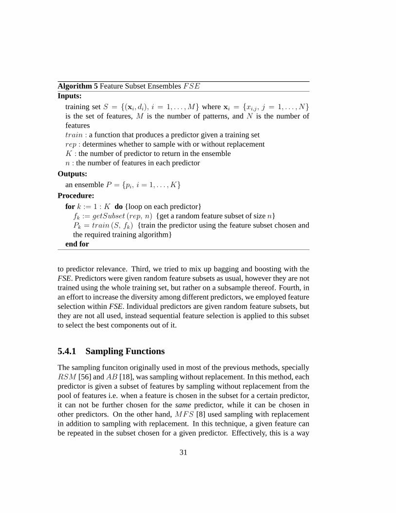
Algorithm 5 Feature Subset EnsemblesFSE
Inputs:training setS = {(xi, di), i = 1, . . . ,M} wherexi = {xi,j, j = 1, . . . , N}is the set of features,M is the number of patterns, andN is the number offeaturestrain : a function that produces a predictor given a training setrep : determines whether to sample with or without replacementK : the number of predictor to return in the ensemblen : the number of features in each predictor
Outputs:an ensembleP = {pi, i = 1, . . . , K}
Procedure:for k := 1 : K do {loop on each predictor}
fk := getSubset (rep, n) {get a random feature subset of sizen}Pk = train (S, fk) {train the predictor using the feature subset chosen andthe required training algorithm}
end for
to predictor relevance. Third, we tried to mix up bagging and boosting with theFSE. Predictors were given random feature subsets as usual, however they are nottrained using the whole training set, but rather on a subsample thereof. Fourth, inan effort to increase the diversity among different predictors, we employed featureselection withinFSE. Individual predictors are given random feature subsets, butthey are not all used, instead sequential feature selection is applied to this subsetto select the best components out of it.
5.4.1 Sampling Functions
The sampling funciton originally used in most of the previous methods, speciallyRSM [56] andAB [18], was sampling without replacement. In this method, eachpredictor is given a subset of features by sampling without replacement from thepool of features i.e. when a feature is chosen in the subset for a certain predictor,it can not be further chosen for thesamepredictor, while it can be chosen inother predictors. On the other hand,MFS [8] used sampling with replacementin addition to sampling with replacement. In this technique, a given feature canbe repeated in the subset chosen for a given predictor. Effectively, this is a way
31
of reducing the number of features chosen as these replicated features add no newinformation to the predictor. We experimented with both sampling techniques, inorder to see the effect of the sampling function on the output of the ensembles.
5.4.2 Weighting Functions
Many of the ensemble techniqes relied on equal weighting of the individual pre-dictors [30]. The predictors have equal votes (in case of classification) or equalweights in averaging (in case of regression). Furthermore, some ensemble tech-niques assigned weights to component predictors relative to their performance,either on the training set or on some validation set [18, 44]. This weighting mech-anism proved useful in some situations, specially in boosting, to give larger em-phasis on better predictors.
We tried out the above two weighting approaches: equal weighting and weight-ing according to predictor performance on the training set. In equal weighting,each predictork was assigned a weightwk = 1
K, whereK is the ensemble size.
In the second method, each predictor’s weight was computed using the softmaxformula:wk = exp(−ek)∑K
i=1exp(−ei)
, whereek is the training error for predictork.
In addition to these two techniques, we used a third weighting mechanism.This relied on the relevance of the features selected for each predictor. Thefeatures in the dataset were ranked according to their relevance [59], employ-ing a variant of sequential forward selection (SFS) algorithm with 10-fold cross-validation. The algorithm stops when all the features are selected in the subset,and bases its estimate of the subset performance on the result of 10-fold cross-validation [60]. Then, each predictor is given a weight according to the ranks ofthe features in its feature subset. The weight given to predictork is defined bywk =
w′k∑K
i=1w′
i
wherew′k =
∑ni=1 ri, ri is the rank of featurei, n is number of
features in each subset, andK is the total number of predictors. This weightingscheme measures the strength of each predictor in terms of the strength of featuresit has. It assigns larger weights to hopefully more relevant predictors, those thathave the most relevant features.
5.4.3 Training Set Subsampling
Training set subsampling has beeen proved effective in creating accurate diverseensembles. The two most successful ensemble techniques, bagging and boosting,are examples of training set subsampling. Therefore, we tried to embed both of
32
bagging and boosting intoFSE, as this has the potential to increase the diversityof the produced ensembles. This seemed attractive, as it combined two orthogonalapproaches, feature set subsampling and training set subsampling, and they bothperform well independently. Hence, we tried to test their behaviour when workingtogether.
When using bagging withinFSE, each predictor gets its own feature subset,and then trains on an independent bootstrap sample drawn from the original train-ing set. The advantage of this approach, like bagging, is that the individual pre-dictors are completely independent of each other, and can be created and trainedin parallel.
On the other hand, using boosting withinFSEis a bit more complicated. Theversion of boosting implemented is ADABOOST.R described in algorithm 2. Afterproviding each predictor with its feature subset, they are trained in sequence, witheach one given a different sample of the training set based on the performance ofthe previous predictors. Those patterns that exhibit higher error with the previouspredictor are given higher probability of beging represented in the sample of thenew predictor. Thus, harder patterns are given more emphasis than easier onesand the predictor can focus its attention to learning those hard-to-learn paterns.
5.4.4 Embedded Feature Selection
We tried yet another technique to help increase diversity ofFSE. In using ran-domly selected feature subset for each predictor, features can get mingled togetherin a way that might worsen that predictor’s performance. Some researchers al-ready used other feature selection techniques for building predictor ensembles,e.g. genetic algorithms [48, 77, 78] and other mechanisms [4, 49]. Hence, wethought of using feature selection after the random feature sampling. In this ap-proach, and after giving each predictor its random share of the features, a fea-ture selection algorithm is applied to choose the best out of those features. Twoalgorithms were tried: Sequential Forward SelectionSFS (algorithm 3) and Se-quential Floating Forward SelectionSFFS (algorithm 4). The former is a simpleand well-established feature selection algorithm. The latter has been proved moreaccurate and stable [58]. The versions of the algorithms employed use 10-foldcross-validation for error estimation and stop when the performance starts to de-teriorate.
33

5.4.5 Feature Subset Selection Criteria
In addition to the above variations to the basicFSE, we tried other systematic fea-ture subset selection criteria. The basicFSEuses random feature subsets for eachpredictor. We thought that having a more advanced feature selection criteria thatcan make use of the knowledge about the features, their relevance and correlation,has the potential of providing better results. Two criteria were tried out for featuresubset selection: feature relevance and feature correlation.
5.4.5.1 Feature Relevance Criteria
Each feature has some inherent strength with respect to the dataset it represents.Knowing those strong features can help us partition the features into strong di-verse subsets. The features relevances are determined as described earlier in sec-tion 5.4.2 using a variant of sequential forward selectionSFS algorithm. Then,this ranked feature list is divided into two equal lists: strong features list and weakfeatures list. Two techniques are employed to select feature subsets for the predic-tors, which we will call pure and hybrid techniques. In the pure technique, eachpredictor takes its subset randomly from either the strong list or the weak list. Halfthe predictors take all their features from the strong list, and the rest take theirsfrom the weak list. On the other hand, each predictor in the hybrid technique takeshalf its subset from the strong list and the other half from the weak list.
5.4.5.2 Feature Correlation Criteria
Correlation between features is a major issue in mahine learning. Using highlycorrelated features adds little information to the learning process. We tried tohave a measure of the corrlation between features, and wanted to roughly dividethem into a group correlated features and antoher of uncorrelated features. Weemployed a heuristic approach to achieve this objective. First, the correlationcorrelation coefficient matrix is calculated for the features from the training set.Then, the features are ranked descendingly according to the abosolute value oftheir mutual correlation. This is achieved by choosing the maximum correlationvalue, extracting the two features intersecting in this value, and adding them to theoutput list. Then, the next highest value is found, and so on. After that, the featurelist is again divided into two equal lists: the correlated list and the uncorrelated list.Likewise, two techniques are used to select feature subsets for the predictors fromthese two lists. In the pure technique, half the predictors take all their features
34

from the strong list and the rest take theirs from the weak list. In the hybrid, onthe other hand, each predictor chooses a mixture of features from the two lists.
5.5 Summary
We followed two approaches in this work. First, comparing basicFSE to othertechniques, both single-predictor and ensemble-based. Second, we added severalvariants to the basicFSEmethod in an attempt to improve its performance. Thesevariations aim at enhancing the performance and accuracy of basicFSE.Theyincluded using another sampling function, weighting functions, adding trainingset subsampling, adding embedded feature selection, and using systematic featureselection methods other than the random feature selection.
35

Chapter 6
Experiments and Results
6.1 Introduction
We carried out extensive experiments in two directions: comparison of theFSEwith other ensemble and non-ensemble techniques, and testing the variations in-troduced to the basicFSE. Three predictor types were used, and several runs wereaveraged to provide the final results stated below. The results emphasized the su-periority of basicFSEwith some predictor types, in addition to the effectivenessof theFSEvariants suggested in this work in improving its performance.
6.2 Experimental Setup
6.2.1 Development Tools
We used Mathworks Matlab 7 R14 as the programming environment for develop-ing the algorithms. We implementedFSE together with its variants,SFS, SFFS,bagging, and boosting. Matlab has built-in implementations forLSE, ANN, andCART trees predictors. Simulations were carried out on a Compaq Proliant MLserver with four Pentium Xion processors at 1.4GHz.
6.2.2 Predictors Types
6.2.2.1 Least Squares Error (LSE)
TheLSE [70] just tries to find the weight vector that minimizes the square errorin mapping the input patterns matrix onto the target vector. GivenX ∈ RM×N is
36

the input matrix withM patterns andN features,d ∈ RM×1is the target vector,LSEfinds the weight vectorw ∈ RN×1 such thatw = (XT X)−1XT d, whereXT
means the transpose of matrixX. This is equivalent to finding the projection ofthe target vector onto the column space of the input matrix. It is clear thatLSEhas no parameters to be set, and is considered the fastest predictor type used inthis work.
6.2.2.2 Artificial Neural Networks (ANN)
Artificial Neural Networks are well known general purpose predictors [53]. Theyhave been successfully used for both classification and regression tasks. There aremany types ofANNwith respect to their training methodology, network structure,number of layers, and interconnections between layers and neurons. The type ofnetworks used here is Feedforward Single Hidden Layer Multilayer PerceptronANNs. They contain an input layer, a single hidden layer, and one output layerwith no feedback connections between neurons. The size of the input layer equalsthe number of features in the dataset, and the output layer contains a single neu-ron. The number of hidden nodes was chosen to be 5 neurons. This size seemedsufficient for the training set size to prevent overfitting. The training algorithmemployed is the Levenberg-Marquardt backpropagation algorithm [46] with de-fault training settings.
6.2.2.3 Classification and Regression Trees (CART)
CART (Classification And Regression Trees) [13] are also general purpose pre-dictors used for both classification and regression. Given a training set, theCARTalgorithm builds a binary tree splitting the space according to the training data.Then, it can get the predicted value of any unknown input by following the pathfrom the root to the leaves of the tree.
6.2.3 Performance Measure
The normal performance measure employed in regression is the mean square er-ror. However, we noticed that this measure depends on the mean of the datasetvalues, and lower means square error in one dataset may be worse than a highermean square error in another dataset. Therefore, we adopted another performancemeasure, namely Normalized Mean Squared Error (NMSE), which is defined by
NMSE =∑
i(yi−yi)
2∑iy2
i× 100 %, whereyi is the predicted value andyi is the target
37

value. This measure normalizes the normal means square error by the square ofthe target value, and so give an error estimate relative to the mean of the dataset.
6.3 Results and Discussions
6.3.1 Comparisons
To be able to get a fair comparison betweenFSEand other techniques, we per-formed more than one run on the datasets. Ten independent runs for each datasetwere performed. In each of the runs, a random subset is chosen from the datasetfor training, with the remaining used for testing. The training set size was cho-sen to be 200 patterns. For each predictor type,FSEswere compared to a singlepredictor using all the features,SFS, SFFS, bagging, and boosting.
Four different ensemble sizes were attempted: 10, 25, 50, and 100. In addition,five different feature subset sizes were tried for FSEs. We tried{0.1, 0.3, 0.5, 0.7, 0.9}×N , whereN is the number of features in the dataset. Hence, 20 different combi-nations were performed for FSE; four different ensemble sizes and five differentsubset sizes for each ensemble size. We experimented with different subset sizesas the effective number of features is dataset dependent, and can not be fixed inadvance.
For these set of experiments, we employed the basic FSE algorithm, whereequal weighting is used and features are selected for each predictor using samplingwithout replacement. This means that a given feature can not be replicated withinthe same predictor, but can be selected for different predictors. Comparison resultsusing LSE predictors are shown in tables 6.1-6.2, whereK respresents the numberof individual predictors, andn denotes the number of features in each individualpredictor of the ensemble. Bold values represent the best result in each technique.Table 6.3 represents a summary for LSE predictors, where the best result for eachof FSE, bagging and boosting is shown. Tables 6.4-6.9 give the correspondingresults forANN andCARTpredictors.
The results reveal some interesting points. First, they show the superiority ofFSEover the other techniques when using the linearLSEpredictor. TheFSEwasfollowed by the sequential selection methods then came the bagging and boosting.Second, they indicate, as expected, that bagging and boosting outperform the othermethods when using non-linear predictors (ANN andCART). This can lend itselfto the non-linear and unstable nature of these predictors. This nature producesmore uncorrelated diverse ensembles, which helps increase their accuracy [14].
38

For theLSE predictor,FSE produced the best results in four out of the sixdatasets, and came the third in the remaining two datasets. Bagging was betterthan boosting in all but one dataset. Sequential selection techniques were alsobetter than bagging in five datasets. Boosting was the worst technique in all thedatasets.
This picture changes considerably when using non-linear predictors such asANN andCART. Bagging and boosting led, on the average, all other techniquesin these experiments. For theANN predictors, boosting was the best predictor infour datasets,FSEin one, andSFSin one. In five datasetsFSEwas the third, andin all the datasets bagging was the second. The sequential selection techniques didnot prove useful with this kind of predictor, but they were, on the average, betterthan the single predictor.
ForCARTpredictors,FSEwas the best in two, and the third in the remaining.Boosting was the best in two, the second in two and the third in two. Bagging wasthe first in two datasets and the second in the rest. Sequential selection methodslagged the other ensemble techniques.
39

Table 6.1: Results for basicFSEs usingLSE predictors, whereK is the ensem-ble size andn is the feature subset size
FSEDataset K
n 10 25 50 100
4 60.52 61.48 62.23 62.5910 52.19 52.76 50.44 51.55
bank32nh 16 45.06 45.77 44.92 44.3122 40.13 39.35 39.85 39.4728 38.83 38.65 38.64 38.374 9.54 9.78 9.93 9.6612 7.73 7.36 7.27 7.21
ailerons 20 5.46 5.70 5.55 5.5328 4.71 4.66 4.56 4.5936 4.41 4.43 4.34 4.378 71.56 71.86 70.10 70.9624 48.18 47.25 46.89 46.36
syn 40 40.85 39.78 39.55 39.1056 40.02 39.10 38.66 38.5872 43.55 43.09 42.72 42.722 39.01 37.82 37.68 37.835 35.08 34.25 34.75 33.81
house16h 8 36.79 35.22 33.69 33.5911 35.77 35.80 35.97 36.1314 39.35 38.90 39.63 39.023 34.49 35.73 35.39 34.398 18.73 18.06 17.67 18.72
comp 11 14.45 10.99 9.96 10.0515 7.05 6.18 6.15 6.1619 4.33 4.35 4.40 4.3555 69.91 69.23 67.81 68.9815 50.44 49.90 50.15 49.27
pole 24 43.28 41.44 41.49 41.2533 41.47 40.71 40.46 40.5143 44.73 44.26 44.50 44.40
40

Table 6.2: Results for other techniques using LSE predictors
Bagging Boosting Single SFS SFFSDataset K
10 40.47 51.46bank32nh 25 40.01 57.87 39.71 38.01 38.05
50 39.81 63.42100 39.79 66.5510 4.42 5.57
ailerons 25 4.36 6.48 4.43 4.35 4.3550 4.39 7.25100 4.37 7.4810 53.62 59.30
syn 25 49.37 56.28 47.81 42.50 43.4650 48.99 54.26100 48.65 53.7210 42.69 88.96
house16h 25 41.72 120.7 41.79 42.98 42.9850 40.86 110.9100 40.68 118.210 4.46 4.68
comp 25 4.47 4.77 4.36 3.77 3.7750 4.45 4.95100 4.44 5.2110 58.76 61.38
pole 25 53.26 47.04 47.43 40.87 41.4150 59.58 43.55100 51.58 43.45
Table 6.3: Comparison results summary using LSE predictors
DatasetAlg. bank32nh ailerons syn house16h comp pole
FSE 38.37 4.34 38.58 33.59 4.33 40.46Bagging 39.79 4.36 48.65 40.68 4.44 51.58Boosting 51.46 5.57 53.72 88.96 4.68 43.45Single 39.71 4.43 47.81 41.79 4.36 47.43SFS 38.01 4.35 42.50 42.98 3.77 40.87
SFFS 38.05 4.35 43.46 42.98 3.77 41.41
41

Table 6.4: Results for basicFSEs usingANNs predictors, whereK is the en-semble size andn is the feature subset size
FSEDataset K
n 10 25 50 100
4 76.85 84.98 65.91 61.7010 68.58 59.21 54.21 51.54
bank32nh 16 82.30 56.62 50.71 44.9222 62.35 46.83 41.71 42.7928 62.08 42.46 41.61 40.814 37.71 12.86 11.86 10.8612 26.73 15.25 10.31 10.67
ailerons 20 18.71 13.30 15.96 7.9028 20.26 8.33 7.19 5.6636 6.08 8.09 6.76 4.828 68.72 112.2 47.58 47.0624 80.40 38.97 33.74 33.56
syn 40 36.19 30.13 28.11 27.1856 31.39 27.39 26.30 25.5372 29.48 26.24 25.44 24.682 33.82 38.92 19167 43.785 162.0 80.84 43.06 50.98
house16h 8 234.1 89.67 57.44 50.6111 251.1 87.68 64.18 58.6814 246.9 75.20 83.39 70.853 7.47 3.31 3.37 2.097 7.43 2.82 1.75 1.53
comp 11 2.05 1.64 1.09 0.6815 0.85 0.56 0.55 0.3619 0.51 5.99 0.29 0.285 2257 41.64 328.8 28.6615 219.9 25.15 27.78 30.38
pole 24 153.0 62.45 26.63 29.8033 81.39 36.31 29.27 33.1543 63.32 37.25 27.83 29.63
42

Table 6.5: Results for other techniques using ANNs predictors
Bagging Boosting Single SFS SFFSDataset K
10 47.02 51.99bank32nh 25 41.75 42.99 113.9 181.9 64.07
50 41.41 39.83100 38.82 38.7810 7.30 5.71
ailerons 25 5.47 4.94 325.1 15.13 12.8650 4.98 4.42100 4.52 4.2110 30.35 31.88
syn 25 26.77 27.06 76.84 65.89 83.1450 26.18 26.18100 25.30 25.2010 76.32 33.89
house16h 25 70.29 26.64 971.3 92.48 103.450 49.85 27.29100 47.77 24.0310 0.94 0.45
comp 25 0.51 0.24 3.67 0.40 0.7250 0.51 0.19100 0.35 0.1810 42.05 676.2
pole 25 33.67 761.5 139.0 11.66 18.9650 27.29 4112100 30.17 2435
Table 6.6: Comparison results summary usingANN predictors
DatasetAlg. bank32nh ailerons syn house16h comp pole
FSE 40.81 4.82 24.68 43.78 0.28 25.15Bagging 38.82 4.52 25.30 47.77 0.35 27.29Boosting 38.78 4.21 25.20 24.03 0.18 676.2Single 113.9 325.1 76.84 971.3 3.67 139.0SFS 181.9 15.13 65.89 92.48 0.40 11.66
SFFS 64.07 12.86 83.14 103.4 0.72 18.96
43

Table 6.7: Results for basicFSEs usingCART predictors, whereK is the en-semble size andn is the feature subset size
FSEDataset K
n 10 25 50 100
4 65.89 64.23 62.83 61.8510 58.05 55.34 54.95 55.08
bank32nh 16 52.31 51.05 50.73 50.1022 53.82 50.32 49.90 49.4328 59.68 57.38 56.87 56.654 10.86 9.96 9.84 9.7412 8.35 8.17 7.87 7.69
ailerons 20 6.98 6.90 6.69 6.6028 6.81 6.57 6.43 6.4336 7.36 7.44 7.29 7.208 85.09 81.06 79.86 78.9524 76.50 70.80 70.09 69.21
syn 40 75.99 71.98 69.90 69.3856 79.76 78.27 75.29 75.6972 101.2 100.3 97.88 97.722 42.07 40.31 39.94 39.535 38.27 36.85 35.84 35.89
house16h 8 38.44 37.39 37.56 36.7011 41.98 40.63 40.68 39.7114 48.65 46.95 47.34 46.823 1.84 1.83 1.59 1.487 0.44 0.39 0.43 0.43
comp 11 0.18 0.20 0.20 0.1915 0.21 0.18 0.18 0.1719 0.22 0.22 0.22 0.225 58.04 53.63 54.52 54.7415 36.75 32.91 32.56 31.82
pole 24 21.48 19.80 20.42 19.2033 14.91 13.51 13.07 13.0243 12.74 11.75 11.72 11.75
44

Table 6.8: Results for other techniques using CART predictors
Bagging Boosting Single SFS SFFSDataset K
10 46.51 51.41bank32nh 25 44.22 46.37 75.98 68.21 68.49
50 43.43 44.84100 43.32 44.0310 5.69 6.27
ailerons 25 5.41 5.53 8.71 9.21 9.2250 5.24 5.30100 5.20 5.2710 73.03 77.19
syn 25 69.07 68.66 130.5 141.1 100.850 68.25 65.32100 67.08 63.4410 40.20 43.49
house16h 25 37.70 41.39 59.18 61.48 52.9250 37.33 40.64100 37.07 40.6910 0.18 2.79
comp 25 0.18 3.47 0.30 0.26 0.2650 0.17 3.30100 0.17 3.1010 10.04 23.48
pole 25 9.49 13.41 14.57 20.43 20.3950 9.45 8.92100 9.20 7.88
Table 6.9: Comparison results summary usingCARTpredictors
DatasetAlg. bank32nh ailerons syn house16h comp pole
FSE 49.90 6.43 69.21 35.84 0.17 11.72Bagging 43.32 5.20 67.08 37.07 0.17 9.20Boosting 44.03 5.27 63.44 40.64 3.10 7.88Single 75.98 8.71 130.5 59.18 0.30 14.57SFS 68.21 9.21 141.1 61.48 0.26 20.43
SFFS 68.49 9.22 100.8 52.92 0.26 20.39
45
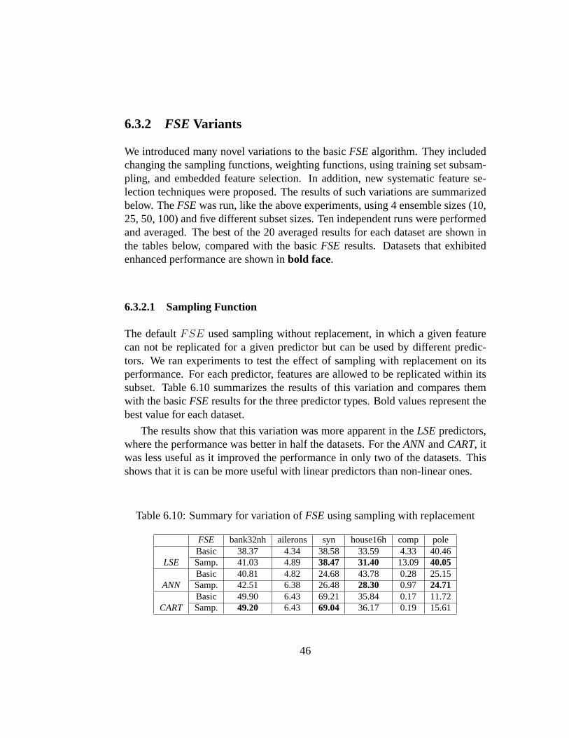
6.3.2 FSE Variants
We introduced many novel variations to the basicFSEalgorithm. They includedchanging the sampling functions, weighting functions, using training set subsam-pling, and embedded feature selection. In addition, new systematic feature se-lection techniques were proposed. The results of such variations are summarizedbelow. TheFSEwas run, like the above experiments, using 4 ensemble sizes (10,25, 50, 100) and five different subset sizes. Ten independent runs were performedand averaged. The best of the 20 averaged results for each dataset are shown inthe tables below, compared with the basicFSE results. Datasets that exhibitedenhanced performance are shown inbold face.
6.3.2.1 Sampling Function
The defaultFSE used sampling without replacement, in which a given featurecan not be replicated for a given predictor but can be used by different predic-tors. We ran experiments to test the effect of sampling with replacement on itsperformance. For each predictor, features are allowed to be replicated within itssubset. Table 6.10 summarizes the results of this variation and compares themwith the basicFSEresults for the three predictor types. Bold values represent thebest value for each dataset.
The results show that this variation was more apparent in theLSEpredictors,where the performance was better in half the datasets. For theANN andCART, itwas less useful as it improved the performance in only two of the datasets. Thisshows that it is can be more useful with linear predictors than non-linear ones.
Table 6.10: Summary for variation ofFSEusing sampling with replacement
FSE bank32nh ailerons syn house16h comp poleBasic 38.37 4.34 38.58 33.59 4.33 40.46
LSE Samp. 41.03 4.89 38.47 31.40 13.09 40.05Basic 40.81 4.82 24.68 43.78 0.28 25.15
ANN Samp. 42.51 6.38 26.48 28.30 0.97 24.71Basic 49.90 6.43 69.21 35.84 0.17 11.72
CART Samp. 49.20 6.43 69.04 36.17 0.19 15.61
46
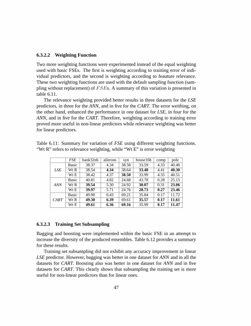
6.3.2.2 Weighting Function
Two more weighting functions were experimented instead of the equal weightingused with basic FSEs. The first is weighting according to training error of indi-vidual predictors, and the second is weighting according to feauture relevance.These two weighting functions are used with the default sampling function (sam-pling without replacement) ofFSEs. A summary of this variation is presented intable 6.11.
The relevance weighting provided better results in three datasets for theLSEpredictors, in three for theANN, and in five for theCART. The error weithing, onthe other hand, enhanced the performance in one dataset forLSE, in four for theANN, and in five for theCART. Therefore, weighting according to training errorproved more useful in non-linear predictors while relevance weighting was betterfor linear predictors.
Table 6.11: Summary for variation ofFSE using different weighting functions.“Wt R” refers to relevance weighting, while “Wt E” is error weighting
FSE bank32nh ailerons syn house16h comp poleBasic 38.37 4.34 38.58 33.59 4.33 40.46
LSE Wt R 38.54 4.34 38.64 33.48 4.41 40.30Wt E 38.42 4.37 38.50 33.99 4.35 40.51Basic 40.81 4.82 24.68 43.78 0.28 25.15
ANN Wt R 39.54 5.30 24.92 30.07 0.31 23.06Wt E 39.97 5.71 24.76 28.73 0.27 23.46Basic 49.90 6.43 69.21 35.84 0.17 11.72
CART Wt R 49.30 6.39 69.61 35.57 0.17 11.61Wt E 49.61 6.36 69.16 35.99 0.17 11.47
6.3.2.3 Training Set Subsampling
Bagging and boosting were implemented within the basic FSE in an attempt toincrease the diversity of the produced ensembles. Table 6.12 provides a summaryfor these results.
Training set subsampling did not exhibit any accuracy improvement in linearLSEpredictor. However, bagging was better in one dataset forANN and in all thedatasets forCART. Boosting also was better in one dataset forANN and in fivedatasets forCART. This clearly shows that subsampling the training set is moreuseful for non-linear predictors than for linear ones.
47

Table 6.12: Summary for variation ofFSEusing training set subsampling. “Bag”refers to using bagging, while “Bst” refers to using boosting
FSE bank32nh ailerons syn house16h comp poleBasic 38.37 4.34 38.58 33.59 4.33 40.46
LSE Bag 38.48 4.39 39.33 55.16 4.68 46.03Bst 51.60 5.52 43.30 100.20 4.79 43.17
Basic 40.81 4.82 24.68 43.78 0.28 25.15ANN Bag 42.97 4.46 39.61 67.36 0.37 44.00
Bst 41.84 4.77 40.13 72.98 0.37 74.61Basic 49.90 6.43 69.21 35.84 0.17 11.72
CART Bag 42.13 5.09 66.17 34.47 0.16 10.98Bst 49.08 5.33 63.57 37.05 0.17 11.28
6.3.2.4 Embedded Feature Selection
Sequential feature selection techniques were employed within the basic FSE tochoose the best feature subset for each predictor. Table 6.13 shows the summaryof these experiments.
The results clearly show that the embedded feature selection was very usefulfor the linearLSE predictors. EmbeddedSFSwas better in four datasets whileembeddedSFFSwas better in five of the six datasets. Likewise, it was also usefulfor the nonlinear predictors. ForANN, it improved the performace in three datasetsfor each ofSFSandSFFS, while in CART it improved the performance in twodatasets for each of the feature selection algorithms.
48

Table 6.13: Summary for variation ofFSE using embedded feature selection.“SFS” refers to usingSFSalgorithm, while “SFFS” refers to usingSFFSalgo-rithm
FSE bank32nh ailerons syn house16h comp poleBasic 38.37 4.34 38.58 33.59 4.33 40.46
LSE SFS 36.21 4.14 38.82 51.11 3.82 38.76SFFS 36.57 4.32 37.54 53.83 3.79 39.13Basic 40.81 4.82 24.68 43.78 0.28 25.15
ANN SFS 39.74 2.15 28.69 42.73 0.32 12.07SFFS 41.73 4.53 27.56 38.16 0.41 10.03Basic 49.90 6.43 69.21 35.84 0.17 11.72
CART SFS 49.77 7.56 85.38 38.89 0.17 12.67SFFS 68.61 7.21 100.1 39.04 0.16 11.19
6.3.2.5 Feature Subset Selection Criteria
Two new criteria, other than random selection, are used in the process of selectingfeature subsets for individual predictors. These are: feature relevance and featurecorrelation criteria.
6.3.2.5.1 Feature Relevance Criteria Features are divided according to theirrelevance into two lists: strong list and weak list. Features are drawn from thesetwo lists using two techniques: either all features come in turn from one of them(the pure technique), or features are selected from both lists (the hybrid tech-nique). In the pure technique, it is apparent that not all the subset sizes are possi-ble, as each predictor is given its subset from half the original number of features,therefore only subset sizes less than or equal to half the total number of featuresare available. Table 6.14 provides a summary of the results.
It is clear from the results that the pure technique did not prove much useful,as it failed to enhance the results in any dataset. However, the hybrid techniquewas more successful. It produced better results in two datasets usingLSE, in twousingANN, and in five usingCART.
49
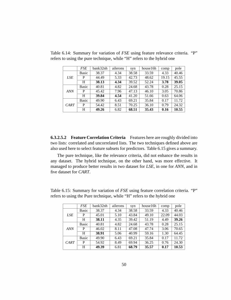
Table 6.14: Summary for variation ofFSEusing feature relevance criteria. “P”refers to using the pure technique, while “H” refers to the hybrid one
FSE bank32nh ailerons syn house16h comp poleBasic 38.37 4.34 38.58 33.59 4.33 40.46
LSE P 44.49 5.33 42.73 48.62 19.15 45.55H 38.13 4.34 39.52 52.24 3.78 39.05
Basic 40.81 4.82 24.68 43.78 0.28 25.15ANN P 45.42 7.96 47.13 46.10 3.05 70.86
H 39.84 4.54 41.20 51.66 0.63 64.06Basic 49.90 6.43 69.21 35.84 0.17 11.72
CART P 54.42 8.51 70.25 36.10 0.79 24.32H 49.26 6.82 68.51 35.43 0.16 10.55
6.3.2.5.2 Feature Correlation Criteria Features here are roughly divided intotwo lists: correlated and uncorrelated lists. The two techniques defined above arealso used here to select feature subsets for predictors. Table 6.15 gives a summary.
The pure technique, like the relevance criteria, did not enhance the results inany dataset. The hybrid technique, on the other hand, was more effective. Itmanaged to produce better results in two dataset forLSE, in one forANN, and infive dataset forCART.
Table 6.15: Summary for variation ofFSEusing feature correlation criteria. “P”refers to using the Pure technique, while “H” refers to the hybrid one
FSE bank32nh ailerons syn house16h comp poleBasic 38.37 4.34 38.58 33.59 4.33 40.46
LSE P 45.01 5.10 43.84 49.10 22.09 44.03H 38.11 4.35 39.42 51.19 4.49 39.26
Basic 40.81 4.82 24.68 43.78 0.28 25.15ANN P 46.02 8.11 47.08 47.74 3.06 70.65
H 38.91 5.06 40.99 59.16 1.30 64.45Basic 49.90 6.43 69.21 35.84 0.17 11.72
CART P 54.92 8.49 69.94 36.25 0.76 24.30H 49.39 6.81 68.79 35.57 0.17 10.53
50
6.4 Summary
Feature Subset Ensembles aim at utilizing all the available features by partitioningthem among the available predictors. We presented here an extensive comparisonwith other single-predictor and ensemble approaches using regression datasets forthe first time. In addition, we investigated several suggested variations to the basicFSEalgorithm, and new systematic partitioning methods. The results proved theeffectiveness of the basicFSEand the success of the added variants in improvingits performance even better.
A summary of all the results is provided here for convenience. Tables 6.17-6.19 brief the results for all the methods used. The naming ofFSEs is accordingto table 6.16. The results clearly show the success of the variations introducedinto the basicFSE. For theLSEpredictors,FSEvariants outperformed the othertechniques in six datasets, whileSFSwas the best in only one. In the six datasetsin which FSEwas superior, the embedded feature selection gave the best resultsin four , while sampling with replacement produced the best in one.
For theANN predictors, boosting was the leader. It outperformed the othersin three datasets, whileFSE was the best in the other datasets. This comes asno surprise, because boosting was reported to outperform other ensemble meth-ods. For theCARTpredictors, boosting again produced good results, but in onlytwo of the datasets.FSE variants were the best in four datasets. The baggingwithin FSEproved very useful, as it produced those four best results. Again thisseems intuitive, as training set subsampling works better for non-linear unstablepredictors.
51
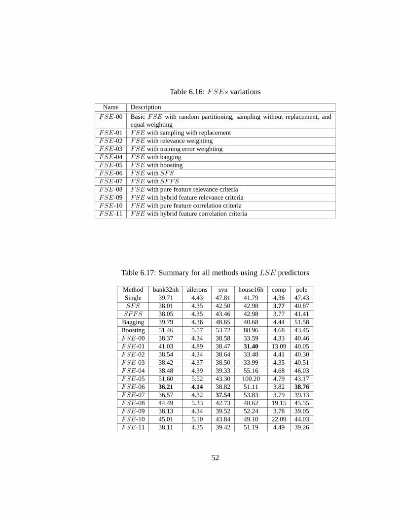
Table 6.16:FSEs variations
Name Description
FSE-00 Basic FSE with random partitioning, sampling without replacement, andequal weighting
FSE-01 FSE with sampling with replacementFSE-02 FSE with relevance weightingFSE-03 FSE with training error weightingFSE-04 FSE with baggingFSE-05 FSE with boostingFSE-06 FSE with SFSFSE-07 FSE with SFFSFSE-08 FSE with pure feature relevance criteriaFSE-09 FSE with hybrid feature relevance criteriaFSE-10 FSE with pure feature correlation criteriaFSE-11 FSE with hybrid feature correlation criteria
Table 6.17: Summary for all methods usingLSE predictors
Method bank32nh ailerons syn house16h comp poleSingle 39.71 4.43 47.81 41.79 4.36 47.43SFS 38.01 4.35 42.50 42.98 3.77 40.87
SFFS 38.05 4.35 43.46 42.98 3.77 41.41Bagging 39.79 4.36 48.65 40.68 4.44 51.58Boosting 51.46 5.57 53.72 88.96 4.68 43.45FSE-00 38.37 4.34 38.58 33.59 4.33 40.46FSE-01 41.03 4.89 38.47 31.40 13.09 40.05FSE-02 38.54 4.34 38.64 33.48 4.41 40.30FSE-03 38.42 4.37 38.50 33.99 4.35 40.51FSE-04 38.48 4.39 39.33 55.16 4.68 46.03FSE-05 51.60 5.52 43.30 100.20 4.79 43.17FSE-06 36.21 4.14 38.82 51.11 3.82 38.76FSE-07 36.57 4.32 37.54 53.83 3.79 39.13FSE-08 44.49 5.33 42.73 48.62 19.15 45.55FSE-09 38.13 4.34 39.52 52.24 3.78 39.05FSE-10 45.01 5.10 43.84 49.10 22.09 44.03FSE-11 38.11 4.35 39.42 51.19 4.49 39.26
52
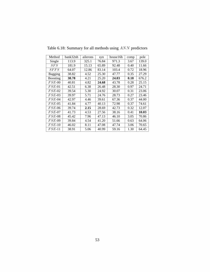
Table 6.18: Summary for all methods usingANN predictors
Method bank32nh ailerons syn house16h comp poleSingle 113.9 325.1 76.84 971.3 3.67 139.0SFS 181.9 15.13 65.89 92.48 0.40 11.66
SFFS 64.07 12.86 83.14 103.4 0.72 18.96Bagging 38.82 4.52 25.30 47.77 0.35 27.29Boosting 38.78 4.21 25.20 24.03 0.18 676.2FSE-00 40.81 4.82 24.68 43.78 0.28 25.15FSE-01 42.51 6.38 26.48 28.30 0.97 24.71FSE-02 39.54 5.30 24.92 30.07 0.31 23.06FSE-03 39.97 5.71 24.76 28.73 0.27 23.46FSE-04 42.97 4.46 39.61 67.36 0.37 44.00FSE-05 41.84 4.77 40.13 72.98 0.37 74.61FSE-06 39.74 2.15 28.69 42.73 0.32 12.07FSE-07 41.73 4.53 27.56 38.16 0.41 10.03FSE-08 45.42 7.96 47.13 46.10 3.05 70.86FSE-09 39.84 4.54 41.20 51.66 0.63 64.06FSE-10 46.02 8.11 47.08 47.74 3.06 70.65FSE-11 38.91 5.06 40.99 59.16 1.30 64.45
53
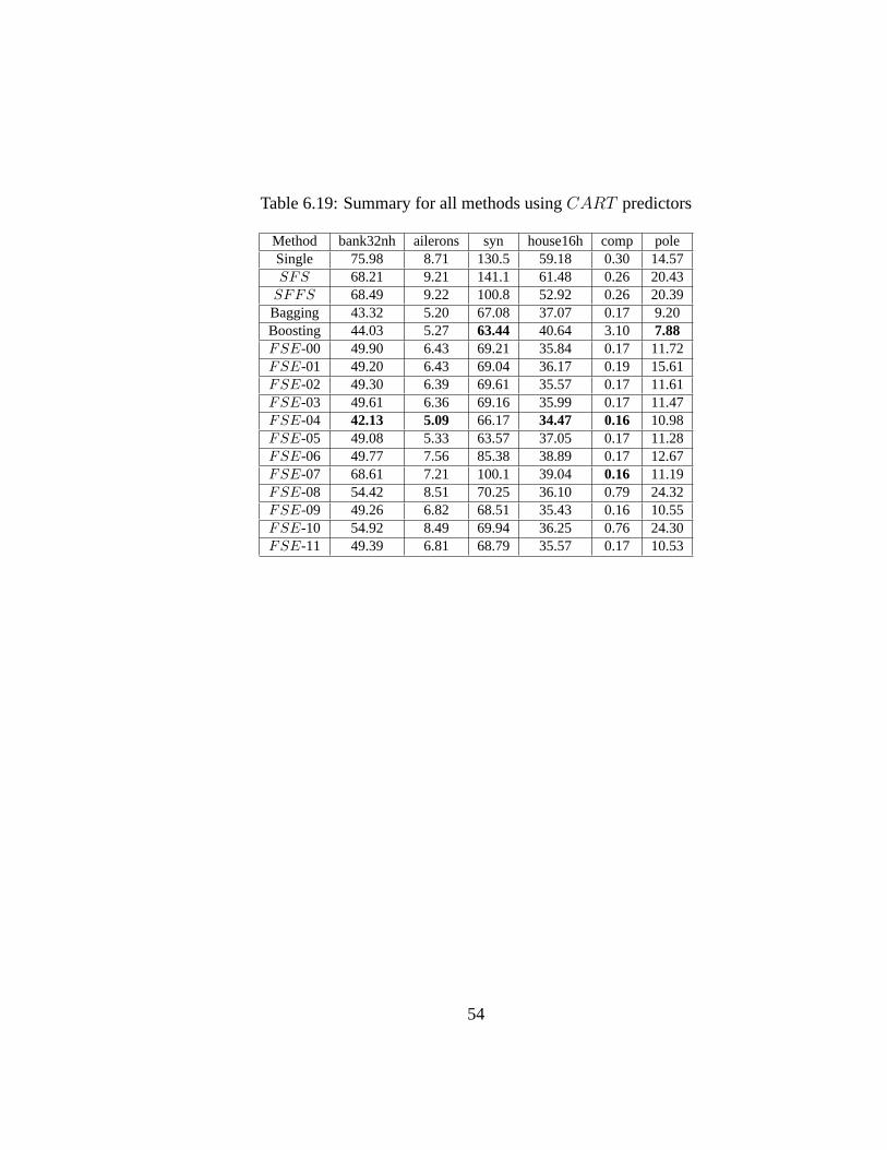
Table 6.19: Summary for all methods usingCART predictors
Method bank32nh ailerons syn house16h comp poleSingle 75.98 8.71 130.5 59.18 0.30 14.57SFS 68.21 9.21 141.1 61.48 0.26 20.43
SFFS 68.49 9.22 100.8 52.92 0.26 20.39Bagging 43.32 5.20 67.08 37.07 0.17 9.20Boosting 44.03 5.27 63.44 40.64 3.10 7.88FSE-00 49.90 6.43 69.21 35.84 0.17 11.72FSE-01 49.20 6.43 69.04 36.17 0.19 15.61FSE-02 49.30 6.39 69.61 35.57 0.17 11.61FSE-03 49.61 6.36 69.16 35.99 0.17 11.47FSE-04 42.13 5.09 66.17 34.47 0.16 10.98FSE-05 49.08 5.33 63.57 37.05 0.17 11.28FSE-06 49.77 7.56 85.38 38.89 0.17 12.67FSE-07 68.61 7.21 100.1 39.04 0.16 11.19FSE-08 54.42 8.51 70.25 36.10 0.79 24.32FSE-09 49.26 6.82 68.51 35.43 0.16 10.55FSE-10 54.92 8.49 69.94 36.25 0.76 24.30FSE-11 49.39 6.81 68.79 35.57 0.17 10.53
54

Part II
Video Traffic Forecasting
55

Chapter 7
Video Network Traffic Forecasting
7.1 Introduction
Multimedia network applications have gained much attention in the past years.Video-on-demand, teleconferencing,IP telephony, and online gaming are justsome of its applications. Multimedia applications need special considerationswhen being transmitted over the network, due to its delay sensitive nature. Someof the applications, e.g. video-on-demand and remote streaming, can tolerate rel-atively high end-to-end delay to allow for edge buffering, a technique used toalleviate the possibility of delay jitter. However, other applications are real-timeand can not withstand this delay, e.g. telephony and teleconferencing. Therefore,destination-side buffering can not be employed here. Other controls have to beused, namely Quality-of-Service(QoS)controls. They assign for each traffic typea certain bandwidth to provide proper delivery to the destination. Nevertheless,they need to know, even roughly, the amount of bandwidth that will be requiredfor the multimedia application. Hence, a robust solution for estimating multime-dia traffic beforehand has to be created.
A major fraction of network traffic involves multimedia applications. Manyresearch papers considered the problem of predicting network traffic. Most of themultimedia traffic comprises video traffic. Video traffic is encoded in many for-mats to convert the huge constant bit rate (CBR) traffic into manageable variablebit rate (VBR) traffic that can be handled efficiently through the network.MPEG(Moving Picture Expert Group) standard is the most widespread compression andcoding method for video streams. Hence, many techniques for predicting networktraffic have been applied to the problem of predictingMPEG-coded video traffic.
56

7.2 MPEG Overview
MPEG is the video compression standard of choice in present applications. MPEGstarted out with MPEG-1 (1992), a standard that aimed to provide video codingfor Video CD-ROMs (VCDs) at 1.5 Mbps. MPEG-2 (1995) was designed laterto provide higher bit rates suitable for High Definition Television (HDTV) at upto 20 Mbps. Later, MPEG-4 (1999) was designed to provide higher quality at bitrates as low as 10 Kbps.
MPEG divides the video stream into a number of pictures, called frames. Twodifferent types of compression methods are used to compress these frames. Intra-frame compression methods can be used to reduce spatial redundancy within thesame frame. Inter-frame compression is employed to reduce the temporal redun-dancy between consecutive frames. These techniques are used to produce threedifferent types of frames:
• I- frames: These are intra-frame compressed frames, where only informa-tion within the same frame is used.I-frames are created with techniquessimilar to JPEG-encoded images. They are considered key frames in the se-quence, allow for random access in the stream, and act as the base for othercompressed frames.
• P-frames: These are predictive frames, where inter-frame motion compen-sated compression is used. They depend on the previousI- or P-frame.
• B-frames: These are bi-directional frames, where bi-directional motioncompensated inter-frame compression is used. The depend on both the pre-vious and nextI- or P-frames, however, they are not used in subsequentpredictions. They provide the highest compression of all the frame types.
The coded frames are then packed into a deterministic periodic sequence, knownas Group of Pictures(GOP). The MPEG specifications do not define the exactorder of the three frame types. However, a typical GOP frame is as shown in figure7.1. The GOP in the figure consists of the sequence “IBBPBBPBBPBB”. EachGOP is characterized by two quantities:M , the distance between two successiveI-frames; andN , the distance between two successiveP-frames. The GOP in thefigure, for example, hasM = 12 andN = 3. As shown, every B-frame dependson the previous and nextI- or P-frame (as expressed by the arrows), and eachP-frame depends on the previousI- or P-frame. The order of transmission is also
57

Figure 7.1: MPEG GOP sequence
I PBB PBB PBB IBB
(a) GOP logical structure
I BBP BBP BBP BBI
(b) GOP order of transmission
shown in the figure, where theI- andP-frames must be transmitted before theirdependentB-frames.
Each of the sequences ofI-, B-, andP-frames have special characteristics.I-frames exhibit the least compression ratios, however, they are the most importantin the GOP, as the remaining frames rely on it. On the other hand,P- andB-framesshow more compression, but they are less important in the GOP. In addition, theyhave different statistical properties, which are used for their prediction. Therefore,when predicting MPEG-coded video, each type of frame is handled separately.
7.3 Literature Survey
Most of the research achieved in multimedia traffic forecasting can be classifiedinto two broad categories. The first deals with the development of stochasticsource models [6, 11, 45, 54, 64]. These approaches model video sources usingHidden Markov chains, statistical techniques, and correlations functions [41]. The
58
second category involves empirical modeling and prediction approaches. There isnot much work done in this category. Many of the proposed empirical modelsare linear. For example, Adas [2, 3] proposes two linear models: a Wiener-Hopfmodel and a Normalized Least Mean Square (NLMS) adaptive model. Yoo [96]develops an adaptive traffic prediction scheme for VBR MPEG video sourcesthat focuses on predicting the effects of scene changes. Both Adas’s and Yoo’sapproaches are adaptive, in the sense that they continually update the predictorweight coefficients with time. Chodorek and Chodorek [24] develop a linear pre-dictor for MPEG-coded video traffic based on partitioning of the phase-space intosub-regions.
Recognizing that nonlinearities in the traffic dynamics are present, a numberof researchers considered models such as neural networks. Chang and Hu [20]implemented a model called Pipelined Recurrent Neural Network (PRNN) for theadaptive traffic prediction of MPEG video signals over ATM networks. Doulamiset al. [33, 34] investigate the application of neural networks for nonlinear trafficprediction of VBR MPEG-coded video sources. In a recent work by Doulamiset al. [35], the authors propose an adaptable neural network architecture that canoperate off-line as well as on-line. In addition, in a recent paper, Bhattacharya etal. [9] proposed a feed-forward and a recurrent neural network model (also see[81]) for the multi-step-ahead prediction (MSP) of MPEG4-coded video sourcetraffic.
7.4 Summary
Multimedia applications are among the most important applications on computernetworks nowadays. Of these applications, real time applications are the mostcrucial. They can not tolerate large delays during transmission. Therefore, strictQoSmeasures are applied to guarantee smooth transfer of data. These measuresrequire accurate prediction for the traffic flow expected out of such applications.
59
Chapter 8
Sparse Basis Selection Approach toVideo Traffic Forecasting
8.1 Introduction
Atiya [5] proposed a novel algorithm for adaptive learnng using Sparse Basis Se-lection. We applied this algorithm to adaptive video traffic forecasting. The mainfeature of the algorithm is its adpatability. It can adapt to changing video char-acteristics, such as changing scene types, or when a new video is presented. Thealgorithm proposed is a novel technology developed in the signal processing co-munity, called Sparse Basis Selection [22, 25, 52, 62, 75, 68, 94]. It is based onhaving a large dictionary of basis signals. Assuming that the basis is combined lin-early, a selection algorithm chooses the most effective small set of basis signals.This technology has almost been confined to the signal processing community,and has applications in signal representation and data compression. The machinelearning community has started exploring these techniques in the last few years,including exploring its relationship with support vector machines [83, 92, 73, 62].
8.2 Sparse Basis Selection
Consider that we would like to represent a signal or a group of signals linearlyin terms of a number of basis functions. The traditional approach has been toconsider a fixed family of basis functions of varying parameters (such as sinusoidswith varying frequencies, or Gaussian functions of varying centers). It wouldbe desirable to have the signal represented by as small set of basis functions as
60

possible. In the sparse basis selection problem we consider a very large dictionaryof possible basis functions (to have a large choice). For example, we can have anumber of functions, such as sinusoids, Gaussians, sinc functions, wavelets, etc.From these we select a set of basis functions as small as possible that can representthe given signal(s) well.
This topic has generated a lot of research activity since the mid nineties. Themain contributions in the early phase of developing the idea can be found in [25,68, 75, 21]. Most of the work has focused on developing efficient algorithms forselecting the best basis functions from among the dictionary functions. Becauseof the combinatorial nature of the problem, it has been shown to beNP-hard, asdemonstrated by Natarajan [75]. Most developed methods produce suboptimalsolutions. A group of methods is based on first selecting the best vector, thenthe vector that together with the previously selected produces the best set and soon. Such approach is termedthe forward greedy selection approach. Anotherapproach,the backward greedy selection approach, starts with the full dictionary,and sequentially eliminates one vector after the other [26].
The problem with the forward selection approach is that once a vector is cho-sen, we are stuck with it and it can not be removed. On the other hand, backwardelimination algorithms are computationaly expensive. A good alternative wouldbe aforward-backwardgreedy approach [73]. In this method, a random subsetof vectors is intilly chosen. Then, at each step, the worst vector is removed fromthis subset and the best vector from the remaining pool is added to the subset.Atiya followed this approach and devised a computationally efficient technique toperform the forward-backward elimination step.
Despite the fact that sparse basis selection produces a linear combination ofthe chosen vector subset, it can be used to produce non-linear prediciton models.This can be accomplished through employing non-linear transformations of theinputs as additional inputs. A number of inputs are extracted from the originaltime series, such as differences, second derivatives, moving averages, absolutedifferences, ...etc. Then, non-linear functions can be applied to these inputs, suchas logarithms, sigmoids, square roots, exponentials, ...etc. By forming a linearcombination of these non-linear transformations of the inputs, we are effectivelyproducing a non-linear model.
61

8.3 Adaptive Sparse Basis Selection
Consider a pool ofK possible inputs. Letx(i) ∈ R1×K andy(i) ∈ R representrespectively the training set input vectors and target outputs (the values to be fore-casted), wherei indexes time. Let the size of the training set beN . Let us arrangethe input vectors in a matrixX ∈ RN×K with the rows beingx(i), and let us alsoarrange the target outputsy(i) in a column vectory. In the sparse basis selectionproblem the goal is to find a small numberJ << K of effective inputs that leadto minimum error. LetS ⊂ {1, 2, . . . , K} denote the set of selected inputs and letS ≡ {1, 2, . . . , K}−S represent the remaining inputs that were not selected. Thedeveloped algorithm is a forward/backward approach. The main steps are givenas
• Initialize with anyJ randomly selected inputsS.
• Remove the element ofS that increases the resulting error the least amount.
• Add the element fromS to S that reduces the resulting error the most.
• Repeat the past two steps until convergence i.e until the removed vector isthe same as the added vector.
The algorithm proposes a faster approach to update the currently selected vectorsand their weights as new data points arrive. It is an adaptive algorithm, in that asnew values arrive they increase the accuracy of the current model in a clever waywithout having to re-calculate everything from scratch. A detailed description ofthe algorithm follows.
8.3.1 Preliminaries
Consider a forward approach, at any step assume we have selected a number ofinputs (corresponding to the columnsXS) with |S| < J , and we would like toselect a vector fromS to add toS. The least square error solution for the weightvector is given as
w = (XST XS)−1XS
T y (8.1)
and the corresponding error is
E = yTP⊥XS
y = yT (I −XS(XST XS)−1XS
T )y (8.2)
62

where the matrixP⊥XS
represents the projection on the null space ofXS. Anefficient way to update the solution vector and compare the contribution of eachvector inS to determine which one to be added toS, is to consider the projectionof XS onto the null space ofXS, defined as
Z = P⊥XS
XS (8.3)
It can be shown that the best element (in terms of minimizing error) to move fromS to S is the one corresponding to columnz of Z that achieves maximum
κ(v) =|zT y|2
‖z‖2(8.4)
A proof will be given in Section 8.3.2.1. Natarajan [75] derived a clever algorithmto update the projected matrixZ every forward selection step to reflect the addedcolumn inXS.
8.3.2 The Forward Update
Assume that at timen − 1 we already have a selected set of inputsS. Also,assume that new measurements are now available at timen, and that we wouldlike to update the setS and its corresponding weight vectorw. To simplify thenotation, let
U ≡ XS (8.5)
V ≡ XS (8.6)
To make the method adaptive and have the recent data have a larger influence onthe selected vectors, we use a discounted error function:
E(n) =n∑
i=1
αn−i[uT (i)w − y(i)]2 (8.7)
whereuT (i) is theith row of U , andα is the discount weight. It is in the rangefrom 0 to 1 (usually close to 1).Let R denote the discount matrix, being ann × n diagonal withRii = αn−i Theprojection matrix is given by
PS = RU(UT RU)−1UT R (8.8)
63

and the minimum error is given by
E(n) ≡ yTP⊥S y = yT
[R−RU(UT RU)−1UT R
]y (8.9)
These formulas are given in a straightforward manner by adapting least squaretheory to the case of a discounted error function.
When new input/output measurements arrive at timen, two tasks have to beperformed. The first task is to examine each of the unselected vectors (the columnsof V ), and find the one vector leading to maximum reduction in error. This, ofcourse, will be done in a computationally efficient recursive manner. The secondtask, once determinining the best vector fromV to add toU , is to update therelevant matrices and variables to reflect this new addition. The algorithms solvingboth tasks are described in the next two subsections:
8.3.2.1 Determining Best Column Vector to Add
The main approach we follow is to compute the formula 8.4 for each of thecolumnsv of V in a recursive manner. This will be described here. Let us com-pute the new error at timen as a function of the error and other variables that areavailable at timen− 1. Define
D(n− 1) = (UT RU)−1 (8.10)
Upon moving forward in time, and getting a new training data point, each ofthe selected basis vectors (the columns ofU ) gets augmented by a new element.Denote the newU matrix as
Unew =
(U
uT (n)
)(8.11)
with U being the old one of timen− 1, anduT (n) being the new added row inU .The discount matrix of timen can be shown to be given by
Rnew = (αR 00T I
) (8.12)
whereR is the old discount matrix and0 = (0 0 . . . 0)T . The newD(n) can bewritten as
D(n) ≡ (UTnewRnewUnew)−1 =
(αUT RU + u(n)uT (n)
)−1(8.13)
64

Using the small-rank adjustment inversion formula [57], we get
D(n) =1
α(UT RU)−1 −
1α2 (U
T RU)−1u(n)uT (n)(UT RU)−1
1 + uT (n)(UT RU)−1u(n)/α(8.14)
For abbreviation, let
b(n) = (UT RU)−1u(n) (8.15)
Then
D(n) =1
αD(n− 1)− b(n)bT (n)
α2 + αbT (n)u(n)(8.16)
TheD(n) is a key variable in the adaptive update. The other two key quantitiesare:
C(n) = XT RX (8.17)
d(n) = XT Ry (8.18)
(rememberX is the matrix consisting of all vectors including selected and unse-lected ones). Upon moving forward in time, all these quantities get updated in astraightforward manner as follows:
C(n) = αC(n− 1) + x(n)xT (n) (8.19)
d(n) = αd(n− 1) + y(n)x(n) (8.20)
wherexT (n) is the new row added to matrixX corresponding to timen data point.These matrices will serve multiple purposes. To be able to extract components
of these, defineCQZ(n) as the submatrix ofC(n) consisting of rows indexed bysetQ and columns indexed by setZ. Of course, each ofQ or Z can be a singlenumber. An analogous definition will apply to the vectordQ(n), and generallythis convention will be used for any matrix or vector.
Assume that we consider adding to the pool of selected inputs an inputiv fromS (corresponding to column ofv of matrixV ) We can rewrite Eq. 8.4 as:
p(v) ≡ vTP⊥S y
vTP⊥S v
(8.21)
65

(noting that(P⊥S )2 = P⊥
S ), and we also have
E ′(n) = E(n)− p(v) (8.22)
whereE(n) andE ′(n) are respectively the error functions before and after addingthe new column. We get
p(v) =vT Ry − vT RUD(n)UT Ry
vT Rv − vT RUD(n)UT Rv(8.23)
We solve for (8.23) in a computationally efficient manner, as follows. First weupdate theC(n) andd(n) matrices with the new data point atn as in (8.44) and(8.45). Then we compute:
A1 = D(n)CSiv (8.24)
A2 = D(n)dS(n) (8.25)
We get
p(v) =div(n)− CT
SivA2
g(v)(8.26)
whereg(v) = Civiv(n)− CT
SivA1 (8.27)
One can see that the above method avoided any computations of orderN . Thelargest computation is of orderK2 (in the update of Eq. 8.44), even after comput-ing p(v) for all possible vectorsv. Another note is that one can use the fact thatD(n) is a rank-one adjustment of the previousD, whetherD of the previous datapointn−1 8.14, orD resulting from a column addition (Eq. 8.32 next Subsection)or deletion (Eq. 8.38 next Section). This can make the computations in (8.47) and(8.25) of orderJ(K − J) rather thanJ2(K − J) (with cycling over allv’s). Wewill not go into the details of this technique, to avoid being too much sidetrackedinto algorithmic details.
Oncep(v) is computed for allv, then the vectorv leading to minimump(v)will be chosen to be added to the setS.
8.3.2.2 Updating the Matrices
Assume columnv of matrix V delivered the lowest resulting error. It is nowrequired to augment the set of selected columnsU with the new additionv, andrecompute all necessary matrices and quantities. LetU ′ be the new augmentedUmatrix. Thus,
66

U ′ = ( U v ) (8.28)
Then, the matrixD(n) can be updated recursively, as will be shown next. LetD′(n) be the updated matrix. It is given by
D′(n) =
(UT RU UT RVvT RU vT Rv
)(8.29)
By the block-partitioned matrix inversion formula, we get
D′(n) =
(UT RU − UT RvvT RU)−1 − (UT RU)−1−UT Rvc
−vT RU(UT RU)−1
c1c
(8.30)
where
c = vT Rv − vT RU(UT RU)−1UT Rv (8.31)
The upper left submatrix in the above matrix can be evaluated using the small-rankadjustment inversion formula. We get
D′(n) =
(UT RU)−1 + (UT RU−UT RvvT RU)−1
c− (UT RU)−1−UT Rv
c
−vT RU(UT RU)−1
c1c
(8.32)
All quantities in the above formula are available as they have been computed inthe previous subsection. We get:
D′(n) =
D(n) +A1AT
1
g(v)A1
g(v)AT
1
g(v)1
g(v)
(8.33)
where everyA1 andv in the formula pertain to the vector that was selected tomove to chosen set.
8.3.3 The Backward Update
In the backward update we eliminate a column vector from the matrix of selectedvectorsU . By eliminating one vector at time, and checking the effect of eachelimination on the error, one can determine the best vector to eliminate. To derive
67

the backward update recursively, we utilize some of Reeves’s formulas [87] for thebackward basis update. Reeves has developed one of the most efficient backwardgreedy algorithms. Reeves showed that upon eliminating column numberk in U ,the error function becomes
Ek(n) = E(n) +
∣∣∣[(UT RU)−1UT Ry]k
∣∣∣2[(UT RU)−1
]kk
(8.34)
whereEk(n) denotes the error after eliminating thekth column,E(n) is the errorbefore eliminating any column, the subscript indexing in the RHS denotes the vec-tor or matrix row/column number (note that we have added the discounting effectto Reeves’s formulas). From the previous section, one see that all the quantitiesneeded here are readily available. For example[
(UT RU)−1]kk
= Dkk(n) (8.35)
whereDkk(n) is kth diagonal element ofD(n). Also,[(UT RU)−1UT Ry
]k
=[D(n)dS(n)
]k
=[A2
]k
(8.36)
We have to computeEk(n) for eachk = 1, . . . , J , and obtain thek that resultsin minimum Ek(n). Once decided which columnk to eliminate, the matricesand quantities used can be updated in a straightforward manner. We will followclosely Reeves’s derivation, adjusting it when needed to reflect the discounting.Let D(n) andD′(n) denote respectively the old value and the updated value of(UT RU)−1. Let us partitionD(n) as follows
D(n) = Π
(Gk gk
gTk Dkk(n)
)ΠT (8.37)
whereΠ represents a permutation matrix that moveskth column andkth row to thelast column and row respectively. The column vectorgk ∈ R(J−1)×1 representsthe kth column ofD(n) with the kth element of that column excluded (that iswithout the diagonal elementDkk(n)). Using the block matrix inversion formulawe get
D′(n) = Gk −gkg
Tk
Dkk(n)(8.38)
68

8.3.4 A Summary of the Algorithm
The algorithm with its forward update and backward update components can besummarized in the following steps:
1. Initialize: Start at timen = n0. Choose the setS randomly as anyJnumbers in{1, . . . , K}. Let S = {1, . . . , K} − S.
2. Compute initial variables:
D(n) = (XTS RXS)−1 (8.39)
C(n) = XT RX (8.40)
d(n) = XT Ry (8.41)
3. Forn = n0 + 1 to N do:
(a) Update the matrices:
D(n) =1
αD(n− 1)− b(n)bT (n)
α2 + αuT (n)b(n)(8.42)
whereb(n) = D(n− 1)u(n) (8.43)
C(n) = αC(n− 1) + x(n)xT (n) (8.44)
d(n) = αd(n− 1) + y(n)x(n) (8.45)
(b) ForI cycles do Steps c) then d):
(c) Backward recursion:Compute
k = argmaxk
[D(n)dS(n)
]k
Dkk(n)k ∈ S (8.46)
Removek from S: S ≡ S−{ k}, S = S∪{ k}. UpdateD(n) accord-ing to Eq. 8.37 and 8.38.
69

(d) Forward recursion:For allk ∈ S:
A1k = D(n)CSk (8.47)
A2 = D(n)dS(n) (8.48)
gk = Ckk(n)− CTSkA1k (8.49)
k = argmaxkdk(n)− CT
SkA2
gk
(8.50)
Move k from S to S: S ≡ S−{ k}, S = S∪{ k}. UpdateD(n) asfollows:
D(n) ≡=
(D(n) + A1kA
T1k
/gk A1k/gk
AT1k
/gk 1/gk
)(8.51)
8.4 Experiments and Results
8.4.1 Video Streams
In our experiments with Atiya’s algorithm, we used MPEG-4 coded video streamsavailable from the Technical University of Berlin [42]. There is a choice ofhigh/medium/low quality movie traces, and we chose the high quality versions.The traces provide the sizes (in bytes) ofI-frames,B-frames, andP -frames. Thetraces were divided into three independent time series:I-frames,B-frames, andP -frames, with different characteristics. Each time series was predicted indepen-dently of other series.
8.4.2 Input Dictionaries
We used the following inputs for the I-frame prediction model (note that the num-bering of the B-frames represents its order in the GOP):1. first backward differenceb(t) = f(t) − f(t − 1) whereb(t) is the input andf(t) is the frame size2. absoulute value of (1)3. exponential of (1) divided by the mean of (2)4. exponential of (2) divided by the mean of (2)5. sigmoid of (1) appropriately scaled, where sigmoid is the function1/(1 + e−x)
70

6. second backward differenceb(t) = f(t)− 2f(t− 1) + f(t− 2)7. spike-detecting input
b(t) =
1 if f(t)− f(t− 1) > mean|f(t)− f(t− 1)|−1 if f(t)− f(t− 1) < −mean|f(t)− f(t− 1)|0 otherwise
8. another spike-detecting input
b(t) =
1 if f(t)− f(t− 1) > std(f(t)− f(t− 1))−1 if f(t)− f(t− 1) < −std(f(t)− f(t− 1))0 otherwise
9. current frame minus the running average of past frames10. a binarization of (9)11-15. difference between two moving average windows, small window with sizes1, 3, 5, 8, and 12 and large window with sizes 2, 9, 15, 24, and 3616. mean of previous 12 frames (including I-, B- and P-frames)17. mean of previous 2 B-frames18. mean of previous 4 B-frames19. mean of previous (B3, B4, B7 and B8) frames20. mean of previous (B1, B2, B5 and B6) frames21. mean of previous 8 B-frames22. previous P-frame23. mean of previous 3 P-frames24. previous I-frame minus mean of 2 previous B-frames25-48. logarithm of (1-24) appropriately scaled49-72. exponential of (1-24) appropriately scaled73-96. square root of (1-24) appropriately scaled97-120. sigmoid of (1-24) appropriately scaled
The inputs for the P-frame model were as follows:1-16. the same as for the I-frames above but applied on P-frames17. previous P-frame minus mean of P-frames18. difference between previous 2 P-frames19. mean of previous 2 P-frames20. mean of previous 2 I-frames21. mean of previous 2 B-frames
71

22. mean of previous 4 B-frames23. mean of previous 8 B-frames24. previous I-frame minus mean of previous 2 B-frames25-48. logarithm of (1-24) appropriately scaled49-72. exponential of (1-24) appropriately scaled73-96. square root of (1-24) appropriately scaled97-120. sigmoid of (1-24) appropriately scaled
The inputs for the B-frame model were as follows:1-16. the same as for the I-frames above but applied on B-frames17. previous P-frame minus mean of P-frames18. mean of previous 2 P-frames19. mean of previous 3 P-frames20. mean of previous (B1,B2) for B1 and B2 frame types, similar input for otherB-frame types21. mean of (B5,B6) for B1 and B2 frames and vice versa, mean of (B7,B8) forB3 and B4 frames and vice versa22. previous I-frame minus mean of I-frames23. mean of previous 2 B-frames24. mean of previous 2 I-frames25-48. logarithm of (1-24) appropriately scaled49-72. exponential of (1-24) appropriately scaled73-96. square root of (1-24) appropriately scaled97-120. sigmoid of (1-24) appropriately scaled
8.4.3 Simulation Results
We used three of the traces: Aladdin, The Firm, and Star Wars IV as a kind oftraining set, to adjust some parameters of the algorithm, such as the adaption rateα, the number of selected basisJ , and the number of iterations for the backwardforward algorithmNITER. Based on these runs we selected these parameters asfollows: alpha = 0.999, J = 5, NITER = 30. We also used the training set todevelop the pool of inputs. Some of the inputs are initially screened for predictivepower using the training set, and are added to the pool if we felt they could beuseful.
We compared the results to those of the neural network prediction model de-veloped by Bhattacharya et al. [9]. We wish to note that if the algorithm is appliedstarting at timen = 1 we will encounter matrix ill-conditioning problems. The
72

reason is that in the outer product matrixUT RU becomes close to singular. Toavoid that, we start at some initial timen0 rather than timen = 1. In that case wewill have to obtain the matrices initially at timen0 by brute force rather than bythe recursive approach (see the algorithm in Section 8.3.4 Eq. 8.39-8.41). Subse-quently, we adapt them according to our recursive algorithm startingn = n0 + 1till the end of the trace (Step 3 in Section 8.3.4). For every video trace we usedn0 equals 500 for the I-frame time series, and equals 2000 for the P-frame and B-frame time series (the total size of the I-frame, P-frame, and B-frame time seriesfor one trace is typically around 7000, 20000, 60000). It is always safer to haven0
large enough. Because no prediction is performed in the interval 1 ton0, we triedto haven0 the smallest possible value that would still be sufficient to avoid theill-conditioning problem. We wanted the excluded initial part as small as possibleto have the comparison with [9] be as fair as possible.
We used a similar error measure as in [9], namely the normalized mean squareerror (it is essentiallySNR−1):
NMSE =
∑Nn=n0
(yn − yn)2∑Nn=n0
y2n
(8.52)
whereyn is the actual time series value,yn is the forecast, andN is the length ofthe trace. We used the following traces as out-of-sample test data for the proposedapproach: Die Hard III, Jurassic Park I, Lecture Room, Mr Bean, Silence of theLambs, Simpsons, and Skiing [42]. Tables 8.1, 8.2, and 8.3 show the predictionresults for respectively the I-frame model, the P-frame model, and the B-framemodel, for all traces including the training and out of sample traces. Also includedin the table are the results whenever available of [9], for comparison. Figures 8.1-8.3 show the prediction versus actual value for a portion of Die Hard III’s I-frame,P-frame, and B-frame time series respectively.
8.4.4 Discussion of the Results
One can see that for most traces the proposed approach produces considerablybetter prediction results than the results in [9]. The improvement is more pro-nounced for the P-frame and B-frame models. The exception is Lecture Room’sI-frame results, where the proposed approach gives 58.3% error. The reason is theill-conditioning problem. It was under control for all other traces, but in LectureRoom apparentlyn0 was not suffiient. In real forecasting situations we can usen0
as large as we want, and therefore the ill-conditioning problem can be completelyavoided.
73

Table 8.1: Prediction Performance for the I-Frame Model (inNMSE)
Trace NMSE(%) [9] (%)Aladdin* 2.50 2.6
Die Hard III 1.89 2.9Jurassic Park I 0.75 0.8Lecture Room 58.3 0.2
Mr Bean 2.22 -Silence of the Lambs 1.61 3.6
Simpsons 1.33 -Skiing 1.12 2.0
Starwars IV* 1.27 1.5The Firm* 1.28 -* indicates traces used for training.
Table 8.2: Prediction Performance for the P-Frame Model (inNMSE)
Trace NMSE(%) [9](%)Aladdin* 9.67 10.3
Die Hard III 4.10 9.0Jurassic Park I 3.36 4.0Lecture Room 1.36 6.9
Mr Bean 6.15 -Silence of the Lambs 4.05 11.0
Simpsons 25.20 -Skiing 2.33 6.2
Starwars IV* 9.05 9.2The Firm* 7.71 -* indicates traces used for training.
74

Table 8.3: Prediction Performance for the B-Frame Model (inNMSE)
Trace NMSE(%) [9](%)Aladdin* 9.25 8.2
Die Hard III 1.51 4.0Jurassic Park I 1.70 2.2Lecture Room 0.72 28.3
Mr Bean 3.08 -Silence of the Lambs 1.53 27.8
Simpsons 10.95 -Skiing 1.10 14.7
Starwars IV* 2.97 3.5The Firm* 1.23 -* indicates traces used for training.
Figure 8.1:I -frame Prediction for Die Hard III
6000 6100 6200 6300 6400 6500 6600 6700 6800 6900 7000
2000
4000
6000
8000
10000
12000
14000
Frame Number
Fra
me
Siz
e
I−Frames for DieHardIII
ActualPredicted
75
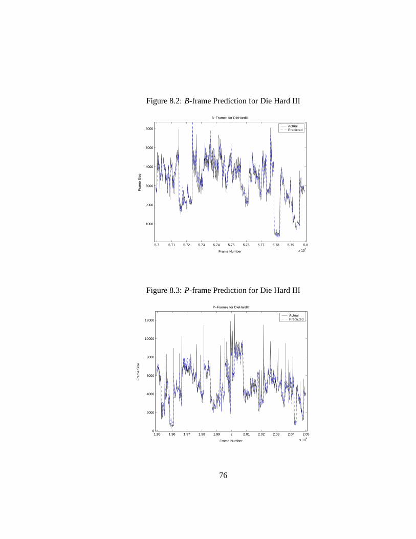
Figure 8.2:B-frame Prediction for Die Hard III
5.7 5.71 5.72 5.73 5.74 5.75 5.76 5.77 5.78 5.79 5.8
x 104
1000
2000
3000
4000
5000
6000
Frame Number
Fra
me
Siz
e
B−Frames for DieHardIII
ActualPredicted
Figure 8.3:P-frame Prediction for Die Hard III
1.95 1.96 1.97 1.98 1.99 2 2.01 2.02 2.03 2.04 2.05
x 104
0
2000
4000
6000
8000
10000
12000
Frame Number
Fra
me
Siz
e
P−Frames for DieHardIII
ActualPredicted
76

8.5 Summary
Sparse basis selection is a robust technique developed in the signal processingcommunity, and was adapted recently to the machine learning arena. We useda novel sparse learning algorithm to adaptively predict video traffic. Adaptabil-ity is in both changing weights of bases selected, as well as the selected basesthemselves. With the addition of each new data point, the set of selected bases isefficiently altered based on the new information available. This technique provedmuch successful and better than currently used prediction methods.
77
Chapter 9
Predictor Ensembles Approach toVideo Traffic Forecasting
9.1 Introduction
Ensemble learning techniques exhibited superior performance in many calssifica-tion and regression tasks. However, it has not been tried in the problem of videotraffic forecasting. We try to focus on the application of video traffic predictionusing predictor ensembles. This is done by considering the video traffic problemas a normal regression task. We tried Artificial Neural Network ensembles, as theyalready showed good performance in video traffic prediction [9]. Three ensembletechniques were used: bagging, boosting, and basicFSE.
9.2 Experimental Setup
9.2.1 Datasets
Video traces from Technical University of Berlin [42] were employed in theseexperiments. We used a subset of the input dictionaries extracted in the experi-ments of Sparse Basis Selection. We discarded the non-linear transformations ofthe generated features, as theANN is already a non-linear predictor and can adjustits weights to cope with the input features. Hence, each dataset is composed of 24features. The features for theI -frames were as follows:1. first backward differenceb(t) = f(t) − f(t − 1) whereb(t) is the input andf(t) is the frame size
78

2. absoulute value of (1)3. exponential of (1) divided by the mean of (2)4. exponential of (2) divided by the mean of (2)5. sigmoid of (1) appropriately scaled, where sigmoid is the function1/(1 + e−x)6. second backward differenceb(t) = f(t)− 2f(t− 1) + f(t− 2)7. spike-detecting input
b(t) =
1 if f(t)− f(t− 1) > mean|f(t)− f(t− 1)|−1 if f(t)− f(t− 1) < −mean|f(t)− f(t− 1)|0 otherwise
8. another spike-detecting input
b(t) =
1 if f(t)− f(t− 1) > std(f(t)− f(t− 1))−1 if f(t)− f(t− 1) < −std(f(t)− f(t− 1))0 otherwise
9. current frame minus the running average of past frames10. a binarization of (9)11-15. difference between two moving average windows, small window with sizes1, 3, 5, 8, and 12 and large window with sizes 2, 9, 15, 24, and 3616. mean of previous 12 frames (including I-, B- and P-frames)17. mean of previous 2 B-frames18. mean of previous 4 B-frames19. mean of previous (B3, B4, B7 and B8) frames20. mean of previous (B1, B2, B5 and B6) frames21. mean of previous 8 B-frames22. previous P-frame23. mean of previous 3 P-frames24. previous I-frame minus mean of 2 previous B-frames
and for theP-frames:1-16. the same as for the I-frames above but applied on P-frames17. previous P-frame minus mean of P-frames18. difference between previous 2 P-frames19. mean of previous 2 P-frames20. mean of previous 2 I-frames21. mean of previous 2 B-frames
79

22. mean of previous 4 B-frames23. mean of previous 8 B-frames24. previous I-frame minus mean of previous 2 B-frames
and for theB-frames:1-16. the same as for the I-frames above but applied on B-frames17. previous P-frame minus mean of P-frames18. mean of previous 2 P-frames19. mean of previous 3 P-frames20. mean of previous (B1,B2) for B1 and B2 frame types, similar input for otherB-frame types21. mean of (B5,B6) for B1 and B2 frames and vice versa, mean of (B7,B8) forB3 and B4 frames and vice versa22. previous I-frame minus mean of I-frames23. mean of previous 2 B-frames24. mean of previous 2 I-frames.
We used the following movie traces: Aladdin, Die Hard III, Starwars IV, TheFirm, Jurassic Park I, Lecture Room, Silence of The Lambs, Skiing, , Mr Bean,and Simpsons. The first four traces were used during training for adjusting theANNparameters, and the remaining six were used as the test set. Each video tracewas divided into three different sequences:I-, B-, andP -frames, and each waspredicted individually. The typical sizes for these traces are 7000, 20000, and60000 for theI -, P- andB-frames respectively. The training set size used was2000, 3500 and 2500 for theI -, P- andB-frames respectively. The rest of eachtrace is used as the test set.
9.2.2 Predictor Setup
We used Artificial Neural Networks for these experiments. The type ofANNsused was Recurrent Multilayer Perceptron (RMLP). They are like normal multi-layer perceptron networks, with the exception that each neuron contains feedbackconnection from its output. This helps to add memory capabilities to the network.They are proved very powerful in modeling complex dynamic systems [81]. Thenumber of input nodes are the number of features selected into each predictor,and the output layer consists of a single neuron. The hidden node contains 3 neu-rons. The networks were trained using the Levenberg-Marquardt backpropagationalgorithm [46] with default training settings.
We experimented with three ensemble techniques in addition to the single pre-
80

dictor. The ensemble methods were: bagging, boosting, and basicFSE i.e. FSEwith random feature subsets and equal weighting. For the ensemble techniques,we tried two ensemble sizes: 50 and 100. For theFSE, we tested for 4 fea-ture subset sizes: 7, 12, 17, and 21. The performance measure used is also theNMSE. The reported results are the average of two independent runs on eachvideo trace.
9.3 Results and Discussion
Tables 9.1-9.3 show the detailed prediction results forI-, B-, andP -frames forthe used movie traces. A summary of the results is presented in tables 9.4-9.6where the best result of each ensemble technique is presented. A comparison withthe sparse basis method and Bhattacharya’s approach [9] is presented in tables9.7-9.9, where only the best ensemble approach is depicted for each trace.
The ensemble results show some points. First, the basicFSEwas the superior,on the average, in the three ensemble techniques used. It was also better thanthe single predictor.FSEwas the best in five datasets for theI -frames, in sevendatasets for theB-frames, and in six datasets for theP-frames. It tied with baggingin one dataset forI -frames, and in three for theP-frames.
Second, the boosting results were worse than bagging for most of the videotraces. Boosting may sometimes suffer from overfitting as a result of focusing onhard examples, which may happen to be noise. It seems that these video tracesare highly unstable, and focusing on such hard patterns leads boosting ensemblesto overfit the data. Third, bagging was the second best technique. It lead in fourdatasets for theI -frames, in two forB-frames, and in one for theP-frames.
The comparison with the sparse and Bhattacharya’s techniques also show thesuccess of the ensemble approach in video traffic prediction. For theI -frames,the ensemble techniques produced comparable, but generally worse, results, as itoutperformed in only two video traces. For theB-frames, the ensemble approachwas apparently more effective. It was the superior in seven traces and the secondbest in one. It was also sucessful for theP-frames, as it produced the best resultsin three traces and was the second best in another two.
81

Table 9.1: Results forI-frame prediction, whereK is the ensemble size andn isthe feature subset size
FSE Bagging BoostingDataset K K K
n 50 100 50 100 50 100
7 5.47 5.5012 5.09 5.02 5.05 4.96 8.31 8.64
Aladdin 17 4.96 4.9121 5.22 5.177 6.34 6.52
Die 12 5.53 5.55 6.01 5.79 9.31 11.49Hard III 17 5.32 5.37
21 5.43 5.417 1.93 1.84
Jurassic 12 1.65 1.65 1.57 1.56 3.48 3.49Park I 17 1.58 1.58
21 1.59 1.587 0.16 0.16
Lecture 12 0.16 0.16 0.15 0.16 0.18 0.19Room 17 0.16 0.16
21 0.16 0.157 6.39 6.3912 6.75 6.36 8.35 8.77 10.38 10.89
Mr Bean 17 8.44 8.1021 9.29 9.367 0.16 0.16
Silence 12 0.14 0.14 0.16 0.17 2.19 2.39of The 17 0.14 0.14Lambs 21 0.14 0.14
7 2.90 2.88Simpsons 12 2.95 2.99 3.82 3.86 3.17 2.98
17 3.28 3.1421 3.74 3.167 4.77 4.82
Skiing 12 4.19 4.14 4.09 4.00 5.37 6.0317 4.05 4.0421 4.03 4.077 4.15 4.11
Star 12 3.59 3.64 3.23 3.25 12.34 11.88Wars IV 17 3.36 3.33
21 3.29 3.317 4.05 4.13
The 12 3.58 3.61 3.26 3.31 11.38 11.17Firm 17 3.39 3.45
21 3.39 3.4082

Table 9.2: Results forB-frame prediction, whereK is the ensemble size andn isthe feature subset size
FSE Bagging BoostingDataset K K K
n 50 100 50 100 50 100
7 7.22 7.0512 5.89 6.06 5.88 5.75 8.60 8.84
Aladdin 17 5.44 5.5621 5.84 5.577 1.17 1.16
Die 12 1.13 1.13 1.14 1.22 2.37 2.18Hard III 17 1.14 1.16
21 1.15 1.167 7.59 7.46
Jurassic 12 7.34 7.44 7.72 7.76 12.98 13.53Park I 17 7.57 7.61
21 8.03 7.987 0.10 0.10
Lecture 12 0.08 0.09 0.09 0.09 0.12 0.14Room 17 0.08 0.09
21 0.09 0.097 5.80 5.8312 5.21 5.43 4.92 4.74 7.35 6.36
Mr Bean 17 5.20 5.2821 5.10 5.127 0.28 0.28
Silence 12 0.27 0.26 0.31 0.30 1.85 1.98of The 17 0.29 0.28Lambs 21 0.31 0.29
7 2.95 2.99Simpsons 12 2.93 2.93 2.94 3.07 3.67 3.96
17 2.93 2.9721 3.02 2.977 1.93 1.92
Skiing 12 1.84 1.84 1.82 1.80 1.99 1.9917 1.81 1.8221 1.84 1.857 0.48 0.47
Star 12 0.50 0.53 1.28 1.07 1.03 0.97Wars IV 17 0.74 0.65
21 0.88 0.827 0.20 0.20
The 12 0.22 0.23 0.26 0.25 0.33 0.30Firm 17 0.31 0.34
21 0.40 0.4583

Table 9.3: Results forP -frame prediction, whereK is the ensemble size andn isthe feature subset size
FSE Bagging BoostingDataset K K K
n 50 100 50 100 50 100
7 11.60 11.5412 11.35 11.31 11.35 11.31 22.79 23.11
Aladdin 17 11.41 11.4321 11.50 11.497 5.77 5.76
Die 12 5.63 5.61 5.59 5.59 16.11 17.02Hard III 17 5.59 5.58
21 5.59 5.597 4.54 4.54
Jurassic 12 4.45 4.45 4.51 4.50 13.00 14.19Park I 17 4.48 4.48
21 4.52 4.537 0.46 0.46
Lecture 12 0.43 0.43 0.41 0.41 0.52 0.61Room 17 0.42 0.41
21 0.40 0.417 8.81 8.7912 9.17 9.13 10.95 10.29 43.54 45.32
Mr Bean 17 9.44 9.5221 9.73 9.747 1.18 1.19
Silence 12 1.15 1.14 1.12 1.12 9.83 9.49of The 17 1.13 1.13Lambs 21 1.12 1.12
7 5.79 5.76Simpsons 12 5.63 5.64 5.68 5.70 14.69 13.88
17 5.64 5.6321 5.66 5.657 7.44 7.43
Skiing 12 7.22 7.18 7.05 7.04 11.97 12.3517 7.12 7.0821 7.08 7.097 7.93 7.92
Star 12 7.83 7.85 7.92 7.95 166.4 155.9Wars IV 17 7.92 7.92
21 7.98 7.977 9.11 9.08
The 12 8.96 8.97 8.96 8.96 58.42 66.93Firm 17 8.96 8.95
21 8.96 8.9784

Table 9.4:I-frame results summary
AlgorithmDataset Single FSE Bag Boost
Aladdin 5.75 4.91 4.96 8.31Die Hard II 5.57 5.32 5.79 9.31
Jurassic Park I 1.66 1.58 1.56 3.48Lecture Room 0.18 0.15 0.15 0.18
Mr Bean 10.34 6.36 8.35 10.38Silence of The Lambs 0.16 0.14 0.16 2.19
Simpsons 4.43 2.88 3.82 2.98Skiing 4.29 4.03 4.00 5.37
Starwars IV 3.40 3.29 3.23 11.88The Firm 4.00 3.39 3.31 11.17
Table 9.5:B-frame results summary
AlgorithmDataset Single FSE Bag Boost
Aladdin 5.88 5.44 5.75 8.60Die Hard II 1.18 1.13 1.22 2.18
Jurassic Park I 8.91 7.34 7.72 12.98Lecture Room 0.11 0.08 0.09 0.12
Mr Bean 5.29 5.10 4.74 6.36Silence of The Lambs 0.34 0.26 0.30 1.85
Simpsons 2.76 2.93 2.94 3.67Skiing 1.88 1.81 1.80 1.99
Starwars IV 0.73 0.47 1.07 0.97The Firm 1.02 0.20 0.25 0.30
85

Table 9.6:P -frame results summary
AlgorithmDataset Single FSE Bagg Boost
Aladdin 11.63 11.31 11.31 22.79Die Hard II 5.63 5.58 5.59 16.11
Jurassic Park I 4.81 4.45 4.50 13.00Lecture Room 0.44 0.41 0.41 0.52
Mr Bean 9.79 9.13 10.29 43.54Silence of The Lambs 1.15 1.12 1.12 9.49
Simpsons 5.77 5.63 5.68 13.88Skiing 7.37 7.08 7.04 11.97
Starwars IV 8.09 7.83 7.92 155.9The Firm 8.98 8.95 8.96 58.42
Table 9.7: I-frame comparison with Sparse Basis Selection and [9]’s method.Bold entries are better than one method, andbold italic are better than the twomethods.
AlgorithmDataset Ensemble [9] Sparse
Aladdin 4.91 2.6 2.50Die Hard II 5.32 2.9 1.89
Jurassic Park I 1.56 0.8 0.75Lecture Room 0.15 0.2 58.3
Mr Bean 6.36 - 2.22Silence of The Lambs 0.14 3.6 1.61
Simpsons 2.88 - 1.33Skiing 4.00 2.0 1.12
Starwars IV 3.23 1.5 1.27The Firm 3.31 - 1.28
86

Table 9.8: B-frame comparison with Sparse Basis Selection and [9]’s method.Bold entries are better than one method, andbold italic are better than the twomethods.
AlgorithmDataset Ensemble [9] Sparse
Aladdin 5.44 8.2 9.25Die Hard II 1.13 4.0 1.51
Jurassic Park I 7.34 2.2 1.70Lecture Room 0.08 28.3 0.72
Mr Bean 4.74 - 3.08Silence of The Lambs 0.26 27.8 1.53
Simpsons 2.93 - 10.95Skiing 1.80 14.7 1.10
Starwars IV 0.47 3.5 2.97The Firm 0.20 - 1.23
Table 9.9: P -frame comparison with Sparse Basis Selection and [9]’s method.Bold entries are better than one method, andbold italic are better than the twomethods.
AlgorithmDataset Ensemble [9] Sparse
Aladdin 11.31 10.3 9.67Die Hard II 5.58 9.0 4.10
Jurassic Park I 4.45 4.0 3.36Lecture Room 0.41 6.9 1.36
Mr Bean 9.13 - 6.15Silence of The Lambs 1.12 11.0 4.05
Simpsons 5.63 - 25.20Skiing 7.04 6.2 2.33
Starwars IV 7.83 9.2 9.05The Firm 8.95 - 7.71
87

9.4 Summary
Video traffic prediction is an important and hard problem. We tried to apply theensemble technique, for the first time, to this application. We used basicFSE,bagging, and boosting.FSEmanaged to outperform the other techniques, baggingcame second, and boosting was the worst. The produced results were encouraging.They were generally worse inI -frame prediction, but generally superior inB- andP-frame forecasting.
88

Part III
Conclusion
89

Chapter 10
Conclusions and Future Work
10.1 Introduction
This work studied the approach of ensemble learning in a regression context. Inthis method, the learning model is composed of a group of predictors instead ofa single predictor. The individual predictors should both be diverse and accurateto provide enhanced performance. Many methods have been proposed to buildsuch diverse, of which bagging and boosting are the most popular and successful.These two methods are based on subsampling the training set while giving all thefeatures to all predictors. A new approach, Feature Subset Ensembles (FSE), thatis based on subsampling the available features is extensively studied in this work.It is comprehensively compared to bagging, boosting, and sequential selectionalgorithms using six regression datasets. In addition, several effective variationsare introduced to the basicFSEalgorithm.
We further discussed an important problem in current network multimediaapplications, namely video network traffic forecasting. It is of crucial importanceto enhancing the quality of service of video transmission over the network. Twoapproaches were used to tackle that problem. The first is using a novel sparsebasis selection algorithm to adaptively predict video traffic. The second is usingthe ensemble approach and treating the problem as a conventional regression task.The two approaches provided encouraging results and outperformed previouslyused methods.
90
10.2 Conclusions
This work provided a comparison of basicFSEwith bagging, boosting, and se-quential selection algorithms. The results showed the success of this technique,both with linear and non-linear predictors. The comparison also asserted the ef-fectiveness of bagging and boosting as two powerful ensemble techniques, andthat bagging can be sometime inferior to boosting but is more stable and resilientto overfitting the training data.
The variations added to the basicFSEwere successful in enhancing its accu-racy, which enabled it to outperform both bagging and boosting on the six useddatasets. The embedded feature selection was particularly successful with linearLSEpredictor, while bagging withinFSEwas helpful with non-linearCARTtrees.
The approach of sparse basis selection to video traffic prediction was also verysuccessful. It applied a novel sparse learning algorithm that recursively updatedthe selected bases and their weights on the arrival of new data. It produced resultssuperior to currently used techniques.
This work also applied the ensemble approach to video traffic forecasting.We tried basicFSE, bagging and boosting. TheFSEproduced the best results,followed by bagging and then boosting. This emphasized the effectiveness ofFSE as a robust ensemble technique. The generated results were encouraging,and outperformed other techniques, including the sparse approach, in many videotraces.
10.3 Contributions
This work introduced many valuable contributions in the area of ensemble learn-ing as well as in the area of video traffic forecasting.
• It provides the first comprehensive comparison of bagging, boosting andFSE in the context of regression problems. The experiments used bothlinear and non-linear predictors and employed six datasets with differentcharacteristics.
• It introdced many valuable variations to the basic FSE algorithm that man-aged to improve its performance for both linear and non-linear predictors.
• These experiments asserted the effectiveness ofFSEand its variants in pro-viding accurate ensembles that can outperform the well-known bagging andboosting.
91

• It introduced the use of sparse basis selection approach to the problem ofvideo traffic forecasting. It employed a novel adaptive approach to solvethis problem, that not only changes the weights of selected bases adaptivelyupon the arrival of new data points, but also changes the selected basesthemselves.
• The sparse basis selection approach provided excellent results on ten differ-ent video traces and outperformed other available methods.
• It introduced the use of ensemble learning approach to the video traffic pre-diction. It used bagging, boosting, and basic FSE, and treated the problemas a regular regression job.FSE, again, was the superior ensemble tech-nique.
• The ensemble approach achieved acceptable results, specially in theB- andP-frame prediction.
10.4 Future Work
Many interesting points arose from this work that deserve further investigation.
• Experimenting with more predictor types, and checking the relation of pre-dictor overfitting to the ensemble performance.
• Adding more enhancements toFSEthat can even improve its accuracy.
• Introducing an automated technique for choosing the bestFSEparameters(size of ensemble and size of feature subset).
• Checking combinations of introduced enhancements, e.g. using training setsubsampling with embedded feature selection.
• Enhancing the video traces dataset and improving the effectiveness of ex-tracted features.
• Improving video traffic prediction accuracy using other, possibly more pow-erful, ensemble approaches or using different predictors.
92

Bibliography
[1] Delve: Collections of data for developing, evaluating, and comparinglearning methods, Computer Science Department, University of Toronto,http://www.cs.toronto.edu/∼delve/index.html, 2004.
[2] A. M. Adas. Supporting real-time VBR using dynamic reservation basedon linear prediction. Technical Report GIT-CC-95/26, Georgia Institute ofTechnology, August 1995.
[3] Abdelnaser M. Adas. Using adaptive linear prediction to support real-timeVBR video under RCBR network service model.IEEE/ACM Transactionson Networks, 6(5):635–644, 1998.
[4] Fuad M. Alkoot and Joseph Kittler. Feature selection for an ensemble ofclassifiers. InProceedings of the4th Multiconference on Systematics, Cy-bernatics, and Informatics, pages 379–384, Orlando, Florida, 2000.
[5] Amir F. Atiya. New adaptive sparse basis selection algorithm. Technicalreport, Cairo University, Giza, Egypt, May 2004.
[6] J. J. Bae and T. Suda. Survey of traffic control schemes and protocols inATM networks. InProceedings of the IEEE ..., volume 79, pages 170–189,1991.
[7] Eric Bauer and Ron Kohavi. An empirical comparison of voting classi-fication algorithms: Bagging, boosting, and variants.Machine Learning,36(1-2):105–139, 1999.
[8] Stephen D. Bay. Combining nearest neighbor classifiers through multiplefeature subsets. InProceedings of the17th International Conference onMachine Learning, pages 37–45, Madison, WI, 1998.
93
[9] Aninda Bhattacharya, Alexander G. Parlos, and Amir F. Atiya. Predictionof MPEG-coded video source traffic using recurrent neural networks.IEEETransactions On Signal Processing, 51(8):2177–2190, August 2003.
[10] C.L. Blake and C.J. Merz. UCI repository of machine learning databases,University of California, Irvine, Dept. of Information and Computer Sci-ences, http://www.ics.uci.edu/∼mlearn/MLRepository.html, 1998.
[11] P. Bocheck and S. F. Chang. A content based video traffic model using cam-era operations. InProceedings of IEEE International Conference on ImageProcessing, pages 817–820, Lausanne, Switzerland, September 1996.
[12] P. Brazdil. Project StatLog, LIACC, University of Porto,http://www.liacc.up.pt/ML/statlog/datasets.html, 1999.
[13] L. Breiman, J. Friedman, R. A. Olshen, and C. J. Stone.Classification andRegression Trees. Chapman and Hall, 1984.
[14] Leo Breiman. Bagging predictors.Machine Learning, 24:124–140, 1996.
[15] Leo Breiman. Using adaptive bagging to debias regression. TechnicalReport TR 547, University of California, Berkeley, California, USA, 1999.
[16] Leo Breiman. Random forests.Machine Learning, 45(1):5–32, 2001.
[17] Gavin Brown, Jeremy Wyatt, Tachel Harris, and Xin Yao. Diversity cre-ation methods: A survey and categorisation.Pattern Recognition Society,2004.
[18] Robert Bryll, Ricardo Gutierrez, and Francis Quek. Attribute bagging: im-proving accuracy of classifier ensembles by using random feature subsets.Pattern Recognition Society, 2002.
[19] M. Burl, U. Fayyad, P. Perona, and P. Smyth. Automating the hunt for vol-canoes on venus. InProceedings of the IEEE Computer Society Conferenceon Computer Vision and Pattern Recognition, pages 302–309, Seattle, WA,1994. IEEE Computer Society Press.
[20] P. R. Chang and J. T. Hu. Optimal nonlinear adaptive prediction and mod-eling of MPEG video in ATM networks using pipelined recurrent neuralnetworks. IEEE Journal on Selected Areas in Communications, 15:1087–1100, August 1997.
94
[21] K. Chen, L. Wang, and H. Chi. Method of combining multiple classifierswith different features and their applications to text-independent speakeridentification. International Journal of Pattern Recognition and ArtificialIntelligence, 11(3):417–445, 1997.
[22] S. S. Chen, D. L. Donoho, and M. A. Saunders. Atomic decomposition bybasis pursuit.SIAM Journal on Scientific Computing, 20(1):33–61, 1999.
[23] Kevin J. Cherkauer. Human expert-level performance on a scientific imageanalysis task by a system using combined artificial neural networks. InPro-ceedings of the13th National Conference on Artificial Intelligence, pages15–21, Portland, OR, 1996. AAAI Press.
[24] A. Chodorek and R.R. Chodorek. An MPEG-2 video traffic predictionbased on phase space analysis and its application to on-line dynamic band-width allocation. InProceedings2nd European Conference on UniversalMultiservice Networks, pages 44–55, April 2002.
[25] R. R. Coifman and M. V. Wickerhauser. Entropy-based algorithms for bestbasis selection.IEEE Transactions on Information Theory, 38:713–718,1992.
[26] S. Cotter, K. Kreutz-Delgado, and B. Rao. Backward elimination for sparsevector subset selection.Signal Processing, 81:1849–1864, 2001.
[27] T. G. Dietterich and G. Bakiri. Solving multiclass learning problems viaerror correcting output codes.Journal of Artificial Intelligence Research,39:1–38, 1995.
[28] Thomas G. Dietterich. Machine learning research: Four current directions.AI Magazine, 18:97–136, 1997.
[29] Thomas G. Dietterich. An experimental comparison of three methods forconscructing ensembles of decision trees: Bagging, boosting, and random-ization. Machine Learning, pages 1–22, 1999.
[30] Thomas G. Dietterich. Ensemble methods in machine learning.LectureNotes in Computer Science, 1857:1–15, 2000.
[31] W. Dillon and M. Goldstein.Multivariate Analysis Methods and Applica-tions. John Wiley and Sons, 1984.
95

[32] J. Doak. An evaluation of feature selection methods and their applicationto computer security. Technical report, University of California, Davis,Computer Science Dept., California, USA, 1992.
[33] A. D. Doulamis, N. D. Doulamis, and S. D. Kollias. Nonlinear trafficmodeling of VBR MPEG-2 video sources. InProceedings IEEE Inter-national Conference on Multimedia and Expo, ICME, pages 1318–1321,July-August 2000.
[34] A. D. Doulamis, N. D. Doulamis, and S. D. Kollias. Recursive nonlinearmodels for on line traffic prediction of VBR MPEG coded video sources.In Proceedings of the IEEE-INNS-ENNS International Joint Conference onNeural Networks IJCNN, pages 114–119, July 2000.
[35] A. D. Doulamis, N. D. Doulamis, and S. D. Kollias. An adaptable neuralnetwork model for recursive nonlinear traffic prediction and modeling ofMPEG video sources.IEEE Transcations on Neural Networks, 14(1):150–166, January 2003.
[36] Harris Drucker. Improving regressors using boosting techniques. InPro-ceedings of the Fourteenth International Conference on Machine Learning,pages 107–115. Morgan Kaufmann, 1997.
[37] Harris Drucker and Corina Cortes. Boosting decision trees. InAdvancesin Neural Information Processing Systems, volume 8, pages 470–485. MITPress, 1996.
[38] B. Efron and R. Tibshirani, editors.An Introduction to the Bootstrap. Chap-man and hall, 1993.
[39] L. Eshelman. The CHC Adaptive Search Algorithm. How to have safesearch when engaging in nontraditional genetic recombination, pages 265–283. Morgan Kaufmann, 1991.
[40] B. Everitt. Cluster Analysis. Heinemann Educational Books, 1974.
[41] Chong Feng, Dan He, and Zhili Sun. A survey on network traffic forecast-ing. In ??, pages ?–?
[42] F. Fitzek and M. Reisselein. Mpeg–4 and h.263 video traces for net-work performance evaluation, Technical University of Berlin, http://www-tkn.ee.tu-berlin.de/research/trace/trace.html, 1998.
96
[43] Yoav Freund and Robert Shapire. A decision-theoretic generalization ofon-line learning and an application to boosting. InProceedings of the2nd
European Conference on Computational Learning Theory, pages 23–37,San Francisco, CA, 1995. Springer-Verlag.
[44] Yoav Freund and Robert Shapire. Experiments with a new boosting algo-rithm. In Proceedings of the13th International Conference on MachineLearning, pages 148–156, San Francisco, CA, 1996. Morgan Kaufmann.
[45] V. S. Frost and B. Melamed. Traffic modeling for telecommunications net-works. IEEE Communications Magazine, pages 70–81, March 1994.
[46] P. R. Gill, W. Murray, and M. H. Wright.Practical Optimization. LondonAcademic Press, 1981.
[47] César Guerra-Salcedo and Darrell Whitley. Genetic search for feature sub-set selection: A comparison between CHC and GENESIS. InProceedingsof the third annual Genetic Programming Conference. Morgan Kaufmann,1998.
[48] César Guerra-Salcedo and Darrell Whitley. Genetic approach to feature se-lection for ensemble creation. InProceedings of Genetic and EvolutionaryComputation Conference, pages 236–243, 1999.
[49] Simon Günter and Horst Bunke. Creation of classifier ensembles for hand-written word recognition using feature selection algorithms. InProceedingsof the8th IWFHR, pages 183–188, Niagara-on-the-lake, Canada, 2002.
[50] L. Hall, K. Bowyer, R. Banfield, D. Bhadoria, W. Kegelmeyer, and S. Es-chrich. Comparing pure parallel ensemble creation techniques against bag-ging. In The Third IEEE International Conference on Data Minin, pages533–536, 2003.
[51] L. Hansen and P. Salamon. Neural network ensembles.IEEE TransactionOn Pattern Analysis And Machine Intelligence, 12:993–1001, 1990.
[52] G. Harikumar, C. Couvreur, , and Y. Bresler. Fast optimal and suboptimalalgorithms for sparse solutions to linear inverse problems.
[53] Trevor Hastie, Robert Tibshirani, and Jerome Friedman.The Elements ofStatistical Learning: Data Mining, Inference, and Prediction. Springer-Verlag, 2001.
97

[54] D. P. Heyman and T. V. Lakshman. Source models for VBR broadcast-video traffic. IEEE/ACM Transactions on Networking, 4:40–48, February1996.
[55] T. K. Ho. Random decision forests. InProc. of the 3rd Int’l Conference onDocument Analysis and Recognition, pages 278–282, Montreal, Canada,August 1995.
[56] Tin Kam Ho. The random subspace method for cosntructing decisionforests. IEEE Transaction On Pattern Analysis And Machine Intelligence,20(8):832–844, August 1998.
[57] R. Horn and C. Johnson, editors.Matrix Analysis. Camridge UniversityPress, Cambridge, MA, 1985.
[58] Anil Jain and Douglas Zongker. Feature selection: Evaluation, applicaiton,and small sample performance.IEEE Transaction On Pattern Analysis AndMachine Intelligence, 19(2):153–158, 1997.
[59] George H. John, Ron Kohavi, and Karl Pfleger. Irrelevant features and thesubset selection problem. InProceedings of the11th International Con-ference on Machine Learning, pages 121–129, San Francisco, CA, 1994.Morgan Kaufmann.
[60] Ron Kohavi. A study of cross-validation and bootstrap for accuracy es-timation and model selection. InProceedings of the International JointConference on Artificial Intelligence, 1995.
[61] Ron Kohavi and George H. John. Wrappers for feature subset selection.Artificial Intelligence, 97(1-2):273–324, 1997.
[62] K. Kreutz-Delgado, J. Murray, B. Rao, K. Engan, T.-W. Lee, and T. Se-jnowski. Dictionary learning algorithms for sparse representation.NeuralComputation, 15(2):349–396, 2003.
[63] Anders Krogh and Jesper Vedelsby. Neural network ensembles, cross vali-dation, and active learning. InAdvances in Neural Information ProcessingSystems, volume 7, pages 231–238, Denver, CO, 1995. MIT Press.
[64] M. Krunz and H. Hughes. A traffic model for MPEG-coded VBR streams.In Proceedings of Joint International Conference on Measurement and
98

Modeling of Computer Systems, ACM SIGMETRICS, pages 47–55, May1995.
[65] Yuansong Liao and John Moody. Constructing heterogeneuos committeesusing input feature grouping: Application to economic forecasting. InAd-vances in Neural Information Processing Systems, volume 12. MIT Press,1999.
[66] Huan Liu and lei Yu. Toward integrating feature selection algorithms forclassification and clustering.IEEE Transaction On Knowledge and DataEngineering, 17(4):491–502, April 2005.
[67] Richard Maclin and David Opitz. An empirical evaluation of bagging andboosting. InProceedings of the14th National Conference on Artificial In-telligence, pages 546–551, Providence, RI, 1997. AAAI/MIT Press.
[68] S. G. Mallat and Z. Zhang. Matching pursuits with time-frequency dictio-naries. IEEE Transactions on Signal Processing, 41(12):3397–3415, De-cember 1993.
[69] U. Marti and H. Bunke. Using a statistical language model to improvethe performance of an HMM-based cursive handwriting recognition sys-tem. International Journal of Pattern Recognition and Artificial Intelli-gence, 15:65–90, 2001.
[70] Carl D. Meyer.Matrix Analysis and Applied Linear Algebra. SIAM, 2004.
[71] J. Moody and J. Utans. Principled architecture selection for neural net-works: Application to corporate bond rating prediction. InAdvances inNeural Information Processing Systems, volume 4. Morgan Kaufmann,1991.
[72] S. K. Murthy, K. Kasif, and S. Salzberg. A system for induction of obliquedecision trees.Journal of Artificial Intelligence Research, 2:1–32, 1994.
[73] P. Nair, A. Choudhury, and A. Keane. Some greedy learning algorithmsfor sparse regression and classification with mercer kernels.Journal ofMachine Learning Research, 3:781–801, 2002.
[74] P. M. Narendra and K. Fukunaga. A branch and bound algorithm for fea-ture subset selection.IEEE Transaction On Computers, 26(9):917–922,September 1977.
99

[75] B. K. Natarajan. Sparse approximate solutions to linear system.SIAMJournal on Computing, 24(2):227–234, April 1995.
[76] L. S. Oliveira, R. Sabourin, F. Bortolozzi, and C. Y. Suen. Feature selectionusing multi-objective genetic algorithms for hand written digit recognition.In Proceedings of the16th ICPR, pages 568–571, 2002.
[77] L. S. Oliveira, R. Sabourin, F. Bortolozzi, and C. Y. Suen. Feature selectionfor ensembles: A hierarchical multi-objective genetic algorith approach. InProceedings of the7th ICDAR, pages 676–680, 2003.
[78] David Opitz. Feature selection for ensembles. InProceedings of the16th
International Conference on Artificial Intelligence, pages 379–384, 1999.
[79] David Opitz and Richard Maclin. Popular ensemble methods: An empiricalstudy.Journal of Artificial Intelligence Research, 11:169–198, 1999.
[80] Nikunj C. Oza and Kagan Tumer. Input decimation ensembles: Decorre-lation through dimensionality reduction. InProceedings of the2nd Inter-national Workshop on Multiple Classifier Systems, pages 210–217, Cam-bridge, UK, 2001.
[81] A. G. Parlos, K. T. Chong, and A. F. Atiya. Application of the recur-rent multilayer perceptron in modelling complex process dynamics.IEEETransactions on Neural Networks: Special Issue on Dynamic RecurrentNeural Networks: Theory and Applications, 5:255–266, March 1994.
[82] Bambang Parmanto, Paul W. Munro, and Howard R. Doyle. Improvingcommittee diagnosis with resampling techniques. InAdvances in NeuralInformation Processing Systems, volume 8, pages 882–888. MIT Press,1995.
[83] T. Poggio and F. Girosi. A sparse representation for function approxima-tion. Neural Computation, 10(6):1445–1454, August 1998.
[84] P. Pudil, F. J. Ferri, J. Novovicová, and J. Kittler. Floating search methodsfor feature selection with nonmonotonic criterion functions. InProceedingsof the 12th IAPR International Conference on Pattern Recognition, pages279–283, 1994.
100
[85] J. R. Quinlan.C4.5: Programs for Mahine Learning. Morgan Kaufmann,1993.
[86] J. R. Quinlan. Bagging, boosting, and c4.5. InProceedings of the13th Na-tional Conference on Artificial Intelligence, pages 725–730, Denver, CO,1996. AAAI/MIT Press.
[87] S. J. Reeves. An efficient implementation of the backward greedy algo-rithm for sparse signal reconstruction.IEEE Signal Processing Letters,6(10):266–268, October 1999.
[88] Amanda J.C. Sharkey, editor.Combining Artificial Neural Nets: Ensembleand Modular Multi-Net Systems. Springer-Verlag, 1999.
[89] W. Siedlecki and J. Sklansky. A note on genetic algorithms for large-scalefeature selection.Pattern Recognition Letters, 10(11):335–347, November1989.
[90] P. Smyth, U. Fayyad, M. Burl, P. Perona, and P. Baldi. Inferring groundtruth from subjective labelling of venus images. InAdvances in NeuralInformation Processing Systems, volume 7, pages 1085–1092, Denver, CO,1995. MIT Press.
[91] S. D. Stearns. On selecting features for pattern classifiers. InThird Inter-national Conference on Pattern Recognition, pages 71–75, Coronado, CA,1976.
[92] J. A. K. Suykens, L. Lukas, and J. Vandewalle. Sparse approximation usingleast squares support vector machines. InProceedings of the IEEE Inter-national Symposium on Circuits and Systems (ISCAS 2000), pages 11757–11760, May 2000.
[93] Kagan Tumer and Nikunj C. Oza. Decimated input ensembles for improvedgeneralization. InProceedings of the International Joint Conference onNerual Networks, Washington, DC, 1999.
[94] K. Wang, C.-H. Lee, and B. Juang. Selective feature extraction via signaldecomposition.IEEE Signal Processing Letters, 4(1):8–11, January 1997.
[95] Ian H. Witten and Eibe Frank. Data Mining: Practical machine learn-ing tools with Java implementations, Morgan Kaufmann, San Francisco,http://www.cs.waikato.ac.nz/∼ml/weka/index.html, 2000.
101

[96] S. J. Yoo. Efficient traffic prediction scheme for real-time VBR MPEGvideo transmission over high-speed networks.IEEE Transactions onBroadcasting, 48:10–18, March 2002.
[97] Meide Zhao, F. Queck, and Xindong Wu. RIEVL: recursive inductionlearning in hand gesture recognition.IEEE Transaction On Pattern Analy-sis And Machine Intelligence, 20:1174–1185, 1998.
[98] Zijian Zheng. Generating classifier committees by stochastically selectingboth attributes and training examples. InProceedings of PRICAI, pages12–23, Berlin, 1998. Springer-Verlag.
[99] Zijian Zheng and Geoffrey I. Webb. Stochastic attribute selection com-mittees. InProceedings of the Australian Joint Conference on ArtificialIntelligence, pages 321–332, Berlin, 1998. Springer.
[100] Zijian Zheng and Geoffrey I. Webb. Stochastic attribute selection com-mittees with multiple boosting: Learning more accurate and more stableclassifier committees. Technical Report TR C98/13, Deakin University,Geelong, Victoria, Australia, May 1998.
[101] Zijian Zheng, Geoffrey I. Webb, and Kai Ming Ting. Integrating boost-ing and stochastic attribute selection committees for further improving theperformance of decision tree learning. InProceedings of the10th IEEEICTTAI, pages 216–223, Los Almitos, CA, 1998. IEEE Computer SocietyPress.
[102] Douglas Zongker and Anil Jain. Algorithms for feature selection: An eval-uation. InProceedings of the International Conference on Pattern REcog-nition, pages 18–22. IEEE, 1996.
102