Engineering Design Calculationswith Fuzzy Parameters

Kristin L. Wood∗

Department of Mechanical EngineeringThe University of Texas at Austin

Kevin N. Otto†

and Erik K. Antonsson‡

Engineering Design Research LaboratoryDivision of Engineering and Applied Science

California Institute of Technology

Received: March 1, 1991Revised: July 13, 1992

Abstract

Uncertainty in engineering analysis usually pertains tostochasticuncertainty,i.e., vari-ance in product or process parameters characterized by probability (uncertainty in truth).Methods for calculating under stochastic uncertainty are well documented. It has beenproposed by the authors that other forms of uncertainty exist in engineering design.Im-precision, or the concept of uncertainty in choice, is one such form. This paper considersreal-time techniques for calculating with imprecise parameters. These techniques utilizeinterval mathematics and the notion ofα-cuts from the fuzzy calculus. The extremes oranomalies of the techniques are also investigated, particularly the evaluation of singular ormulti-valued functions. It will be shown that realistic engineering functions can be usedin imprecision calculations, with reasonable computational performance.

1 Introduction

1.1 Uncertainty in Engineering Design

Engineering design may be viewed as a goal-directed process, with the generally recognizedstages of synthesis, evaluation, and decision [1, 3]. Other authors [19, 21] define engineeringdesign, instead, as a mapping of the functional description of an artifact or process to a formdescription. While these definitions focus on different aspects of design as a human activity,each implicitly assumes the need to compare and contrast alternative designs.

During the preliminary design stages, design alternatives are usually described only ap-proximately or imprecisely. Precise geometry, material properties, manufacturing processes,

∗Assistant Professor†Graduate Research Assistant‡Associate Professor, Mail Code: 104-44, Caltech, Pasadena, CA 91125

1

etc., are not specified or known. Conventional computer-aided design methods require highlyprecise descriptions in order to operate, making them difficult or impossible to use during theearly design process. This research focuses on the development of methods for representingand manipulating imprecise descriptions of designs to provide the designer with more infor-mation to compare alternatives during the preliminary design phase.

Using this premise, what types of uncertainty are encountered in preliminary design? Howcan we compute under uncertainty? Engineering design uncertainty is comprised ofdesignimprecision(uncertainty in choosing among alternatives) andstochastic uncertainty(usuallypertaining to manufacturing and measurement limitations) [23]. Stochastic uncertainty arisesfrom a lack of exact knowledge of a parameter due to some process the designer has no di-rect control or choice over. A manufacturing tolerance is an example of such an uncertainty.Stochastic uncertainties are usually represented and manipulated using the probability calculus(Cox [5], Jeffreys [11]).

Design imprecision, on the other hand, concerns the choice of design parameter valuesused to describe an artifact or process. For example, in the preliminary design of equipmentfor processing solid epoxy resin, pumps feed molten resin to an extrusion/applicator head. Theapplicator head conducts the molten resin to a belt assembly, which compresses and conveys theresin in sheet form through a chilling process. A thrasher then chops the sheets into “flakes”for storage and transportation. Although the process layout is well defined in this case, theapplicator and thrasher designs are imprecisely described, depending on the geometry, thermal,fluid, and other material properties of the resin. Given alternative designs for the applicator andthrasher, how can these alternatives be compared with respect to the imprecision?

We use the designer’s preference to quantify the imprecision with which design parametersare known. Preference, as used here, denotes either subjective or objective information thatmay be quantified and included in the evaluation of design alternatives. For instance, an ap-plicator design for the resin flaking process may include a wide range of material choices forthe applicator’s head structural supports. Preference of the material choice will depend on thecorrosion and thermal expansion properties. The following section describes a general methodfor representing and manipulating this type of information in engineering design calculations.

1.2 General Approach

In this research, we pursue asemi-automatedapproach to the design of such complex entities asa process. That is, we propose to aid the designer’s ability to make decisions in the preliminarydesign stage. The salient feature of this part of the preliminary design stage is uncertainty in themodel used. We model and manipulate such uncertainties in a computer-assisted environment,under the hypothesis that doing so will allow the designer to make faster and more-informeddecisions.

The model implies the designer arrives at candidate solutions by the designer’s own creativeinferencing, using, for example, traditional techniques of divergent thinking [1, 22]. Yet thesemodels so determined are not completely described, and the designer cannot determine whichcandidate offers the best alternative to pursue into the subsequent, expensive detailed-designstage.

Graphically, our computational model of the design process is depicted in Figure 1, calledthe Method of Imprecision. At the start of the process, the designer suggests possible solu-tions. These are subsequently transformed into formal candidate solution models upon whichcomputations can be performed. Each model includesdesign parameters, di, variables to bedetermined during the design process, andperformance parameters, pj, variables (parame-

2

u1, u2, ..., un

aImprecise Preference Functions

Model Interpretation

Model Formalization

The Imprecision Transformation

1 m

n21

pp

ddd

Preliminary Design Decisions

Physical Space Design Parameters

a a a

. . .

a a

. . .

Figure 1: The Method of Imprecision.

3

terized as functions of the design parameters) used to give an indication of the performanceachievable by the design.

Having determined conceptual models of the proposed candidates, the designer then spec-ifies the design parameters imprecisely. The degree to which a designer prefers a value of adesign parameter shall be denotedµ, termedpreference. This is a normalized ranking of thedesigner’s belief that the value will be used in the design. The specification ofµ (how mucha design parameter value will possibly satisfy the design) is based on the same foundations asused by the designer to hypothesize typical values. Usually this information comes from objec-tive sources such as corrosion data, geometric constraints, or material properties. It also comesfrom subjective sources as well, such as the belief in availability of components or impreciseknowledge of reliability. Imprecise specifications explicitly represent these forms, allowing thedesigner to justify preliminary design decisions.

Having performed this formalization, theImprecision Transformationis invoked to calcu-late the imprecise achievable performance. This calculation is performed over theentire setof imprecise values specified, allowing the designer to make more informative evaluations. Ithas been shown that using the fuzzy mathematics is a well suited method for imprecise designcalculations [25], rather than, for example, using the probability mathematics. The fuzzy math-ematics preserves peak preferences on the performance parameters with peak preferences onthe design parameters, a required feature for the transformation. The imprecision transforma-tion is based on Zadeh’sextension principle[27] to calculate the preference of any performanceparameter valuepj:

µ(pj) =

{sup {min {µ(d1), . . . , µ(dN )} | d1, . . . , dN : pj = fj(d1, . . . , dN )}

0 if {d1, . . . , dN | pj = fj(d1, . . . , dN )} = ∅ (1)

whered1, . . . , dN are values of the imprecise design parameters,pj = fj(d1, . . . , dN ) is aperformance parameter expressed as a function of the design parameters, andµ(di) is thedegree of preference for the design parameter valuedi used.

After having made the performance parameter preference calculations, the designer canobserve the imprecise performance achievable and proceed to judge the candidates. With sin-gle performance parameter designs, this process involves determining the preference of theperformance parameter at the one required performance value (thefunctional requirement).With multiple performance parameter designs, afigure of meritmust be introduced to combinethe different performance parameter preferences at each performance parameter’s functionalrequirement level. This involves trading off conflicting goals and is beyond the scope of thisdocument, but the interested reader should refer to [23, 26].

The design paradigm presented so far assumes the preliminary design process can be car-ried out in a forward manner. Of course, there will be iteration among the steps presented.Observations in the achievable performance will induce changes in the specified preferencesfor design parameter values. Hence there is a need for real-time calculation of the performanceparameter preferences induced from the design parameters. The next section will present acomputational model for evaluating the preference functions of performance parameters, in-troduce a more efficient algorithm for a restricted class of problems, and introduce an newalgorithm for more general functions involving extrema.

4

2 The Computational Model for Design Imprecision

2.1 Introduction

Previous publications [23, 24, 26] present a methodology by which uncertainties in preliminaryengineering design can be represented and manipulated. This section discusses the componentof the methodology that requires the computation of Zadeh’sextension principle[27], i.e.,fuzzy arithmetic for the purpose of this study. The entire computational structure and require-ments for implementing the methodology, including equation parsing, symbolic manipulation,and so on, is beyond the scope of this document.

2.2 Computation of the Extension Principle

Kaufmann and Gupta [12, 23] describe an analytical method of calculating a fuzzy output(application of Zadeh’sextension principle) from imprecise inputs. This method is based onα-cuts [12] and interval arithmetic [14]. Although the method is straight-forward in its ap-proach, the manipulation of symbols and the solution of expressions that include high orderpolynomials, both in the numerator and denominator (for extended division), make this methodinfeasible for computer-assisted design applications. This is compounded by the fact that theexact solution to the analytical application of theextension principlecan be shown to be equiv-alent to an unwieldy non-linear programming problem [2]. A discrete numerical approach istherefore necessary to meet the computational requirements for handling many design param-eters. This section will discuss a useful numerical technique, the LIA algorithm, and introducea number of extensions.

2.2.1 The LIA Algorithm

In reviewing the literature, many discrete and analytical methods exist for carrying out ex-tended operations with fuzzy sets (or fuzzy numbers). The Fuzzy Weighted Average (FWA)algorithm, as presented by W.M. Dong and F.S. Wong in [7], outlines a simple and efficientalgorithm that is useful for carrying out engineering design calculations. We extend this algo-rithm below for generalized real functions of fuzzy variables, referring to the extended formas thelevel interval algorithm(LIA). Comparing the algorithm to the analytical method out-lined in [12], LIA uses the interval analysis techniques as described; yet, LIA simplifies theprocess extensively by discretizing the membership functions of the input fuzzy numbers intoa prescribed number ofα-cuts. Performing interval analysis for eachα-cut and combining theresultant intervals, the output is a discretized fuzzy set, the performance parameter output ofinput preference functions for the case of a design calculation. Dong and Wong also includea combinatorial interval analysis technique in order to avoid the problems of the multiple oc-currence of variables for division and multiplication in an algebraic equation expression. Acondensed version of the algorithm from [7] has been provided below (where the terminologyhas been changed to reflect the application to design calculations). Later sections will describethe implementation and extension of this algorithm; hence its inclusion in this paper.

There are conditions which must be satisfied for application of the algorithm: the prefer-ence functions must satisfy the normality and convexity conditions and must be continuousover d; no singularities of the functions can occur overd (i.e., no division by zero can occur,and no zero arguments can occur infj(~d) for eachdi for the unary operations, such as thenatural logarithm and the square root); and only monotonic regions of multi-valued functions,

5

Table 1: Design Parameter Data for Column Equation.DPs (units) α = 0 α = 1 α = 0n 1.0 3.0 5.0l/r 60.0 100.0 160.0E (GPa) 75.0 150.0 225.0K (simply-supported) 1.0 1.0 1.0

e.g., sine and cosine, are computed for a givendi.1

The algorithm is as follows: forN real imprecise design parameters,d1, . . . , dN , let di

(i ∈ [1,N ]) be an element ofdi. Given a performance parameter represented by the mapping

p = f(d1, . . . , dN ) ∀di ∈ di

respectively, letP be the fuzzy output of the mapping. The following steps lead to the solutionof P .

1. For eachdi, discretize the preference function into a number ofα values,α1, . . . , αM ,whereM is the number of steps in the discretization.

2. Determine the intervals for each parameterdi, i = 1, . . . ,N at eachα−cut, αj , j =1, . . . ,M .

3. Using one end point from each of theN intervals for eachαj , combine the end pointsinto anN -ary array such that2N distinct permutations exist for the array.

4. For each of the2N permutations, determinepk = f(d1, . . . , dN ), k = 1, . . . , 2N . Theresultant interval for theα−cut,αj, is then given by

Pαj = [min(pk),max(pk)].

For N imprecise design parameters andM discrete preference levels, the complexity ofthis algorithm is given by

H ∼ M · 2N−1 · κ (2)

whereH equals the number of operations andκ equals the number of multiplications anddivisions inf(~d). Figure 2 shows the results of the analytical application of theextensionprinciple to the column-stress equation (Equation 3), along with the results using LIA.

σa =π2E

n(

Klr

)2 . (3)

The input parameters for the maximum allowable stressσa (Equation 3) are triangular prefer-ence functions as listed in Table 1. No noticeable differences can be seen in the figure; however,minimal error is of course encountered due to discretization and the precision of the computerused.

1Reference [23] discusses methods for relaxing the continuity and monotonicity conditions offj(~d).

6

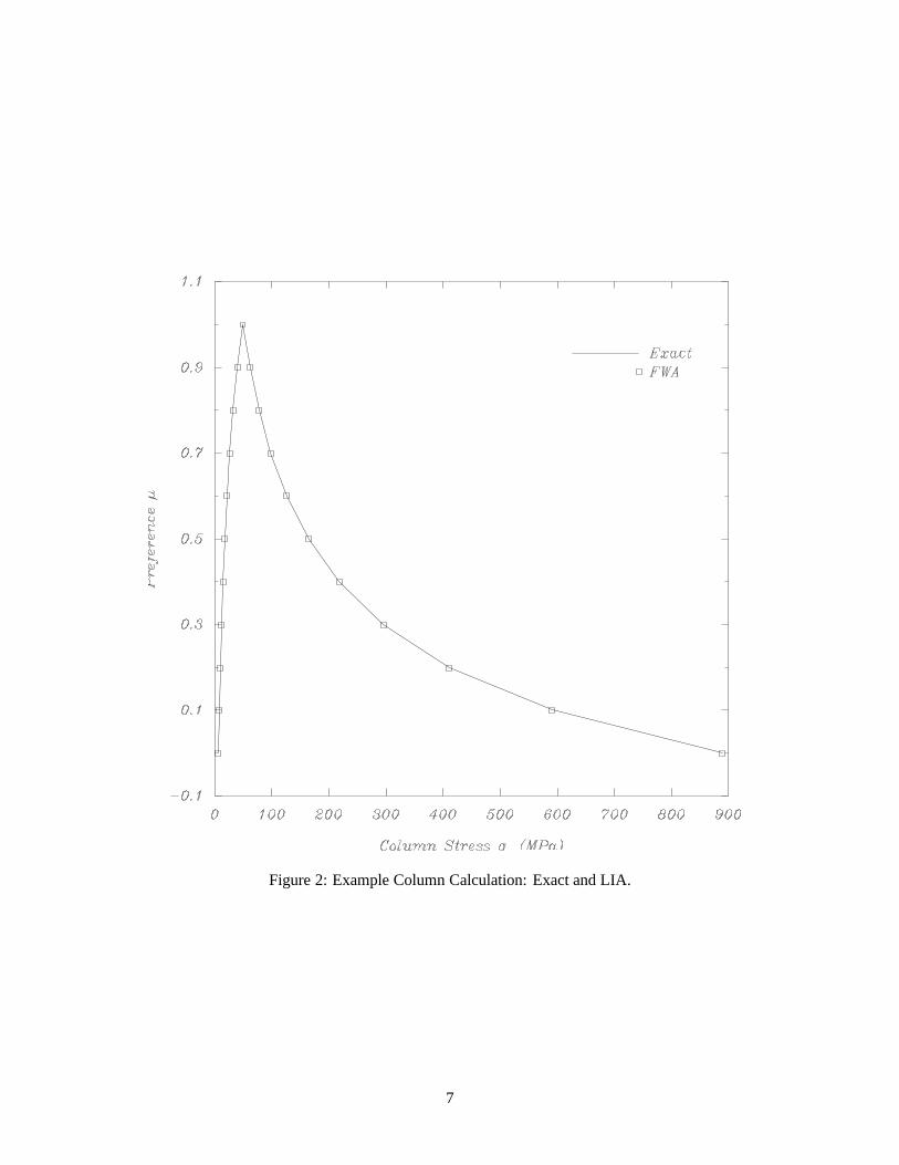
Figure 2: Example Column Calculation: Exact and LIA.

7

2.2.2 Implementation Scheme for LIA

For the LIA to be an efficient tool within real-time computer-assisted design, the implementa-tion scheme must be considered in detail. A computationally efficient implementation of Dongand Wong’s algorithm [7], written in pseudo-code, is shown in Figure 3.

The input arrayd contains the discretized elements for each input design parameter. Forexample, given two parameters,d1 andd2, and threeα-cuts,α = 0.0, α = 0.5, andα = 1.0,thed array is expressed as follows:

d = [d11, d12, d13, d14, d15, d16,d21, d22, d23, d24, d25, d26]

where the first index corresponds to the parameter number and the second to the elements in theparameter’s support due to theα-cuts. Figure 4 illustrates two (out of many possible) examplesof fuzzy parameters (preference functions) that can be expressed in thed array.

Considering the implementation scheme further, another array (integer mask), is estab-lished in order to step through thed input array. The method consists of a bitwise system todetermine the offset into the array. Employing this method conserves memory. Besides themasking system, the routinefunc() contains the actual algebraic expression, in the form of abinary tree, to be solved to obtain the fuzzy output. Infunc(), standard software engineeringand symbolic programming rules are applied to reduce the number of multiplications. Suchrules have lead to theconsts() function seen later in the code, which multiplies the result byany constants in the original expression that were not necessary in evaluating the variablesfminandfmax. The routineconsts() may save at least2N multiplications and/or divisions, where Nequals the number of fuzzy parameter inputs. Finally, thefwa() scheme calls another routine,table vals(). table vals() constructs a look-up table of the input parameters that form the dis-crete outputs lying on the actual membership curve at theα-cut levels (used to determine whichinputs combined to give a particular value in the output performance curve). Interpolation maybe employed to determine the values of the corresponding inputs for other points on the curve.

The algorithmic complexity of the implementation (repeated from Equation 2) may bedetermined. ForN design parameters, the complexity is of order

H ∼ M · 2N−1 · κ

whereH equals the number of operations andκ equals the number of multiplications anddivisions in the routinefunc(). From a practical standpoint, a minicomputer or workstation ex-ecutes this routine (binary operations only infunc()) essentially in real-time for at least fifteenfuzzy input parameters for one equation. When adding trigonometric functions to the expres-sion in func(), a time delay of seconds becomes apparent for around ten inputs.2 Overall, thecomplexity result demonstrates the relative efficiency of LIA and its implementation scheme.

2.2.3 Revising the LIA Approach

Reducing the Complexity In the previous sections of this paper, the LIA algorithm for de-sign calculations was presented in detail. Extensions to the algorithm in terms of implemen-tation and reducing the complexity of the functional expression have been shown. Althoughthe extended algorithm, as it stands, is usable forreal-timeengineering design calculations,

2These qualitative comments are generalizations of benchmarks taken from a Sun Microsystems 4/330 work-station. Of course, the comments here will vary somewhat depending on the expression infunc().

8

Inputs:(1) d, array of elements of input parameters.(2) N, number of fuzzy input parameters.(3) M, number of discrete points.

Outputs:(1) p, array containing imprecise result,p = f(d1, . . . , dN ).

extended-calculation(d,N,M)

BEGINinteger ialphacuts, i, j,

l, j lim, icut, ioffset;integer mask[noof input parameters];real fvar[noof input parameters],

f, fmin, fmax;

ialpha cuts = M / 2; /* No. of alpha cuts. *//* Create the bit masks to retrieve a value in the d array.*/for i = 0 to (N-1)

mask[i] =2i;for icut = 0 to (ialphacuts-1)BEGIN

for i=0 to N-1fvar[i] = d[i*M+icut];

fmin = func(fvar,N);fmax = fmin;j lim = 2N − 1;for j=1 to j limBEGIN

for l=0 to (N-1)BEGIN

if((mask[l] AND j) == mask[l])ioffset = M - icut - 1;

elseioffset = icut;

fvar[l] = d[l*M+ioffset];END;f = func(fvar,N);fmin = min(fmin,f);fmax = max(fmax,f);table vals(f,fmin,fmax,fvar,N,M,icut);

END;consts(fmin,fmax);p[icut] = fmin;p[M-icut-1] = fmax;

END;return results in p[], with impliedα values from ialphacuts;

END;

Figure 3: Extended Operations Algorithm: Pseudo-Code.

9

a1 = 0.0

a2 = 0.5

a3 = 0.0

a1 = 0.0

a2 = 0.5

a3 = 1.0

a

a

d26d25d24d23d22d21

0.0

d15

d14d13d12 d16d11

0.0

d

0.5

1.0

1.0

0.5

d

Figure 4: Example of the d Array.

10

its complexity can be reduced further. Adapting interval analysis methods [14] to theα-cutformulation of the algorithm is the key to the reduction in complexity.

Certain definitions and theorems as presented by Moore [14] are needed to construct andexplain the reduction in complexity of the LIA algorithm (as developed in this document).These definitions and theorems are provided in Appendix A, where Moore [14] can be refer-enced for the details and proofs.

Applying the Methods of Interval Analysis Using engineering design terminology andnomenclature, the problem is to compute the performance parameter resultspj, j = 1, 2, . . . ,mat eachα-cut for a class of real-valued design functionsDF (X0), wherepj = f(d1, d2, . . . , dn),andXα denotes the support of anα-cut across the design parameters. TheDF (X0) composethe arithmetic functions{+,−, /, ·} and unary functions{sin(·),cos(·), exp(·),ln(·),√·, etc.},i.e., all standard computing functions. Assuming that a functionf in the class of functionsDF (X0) is defined for allD ∈ X0, and assuming that no division by zero or unary opera-tion of zero for{ln(·) or

√·} occur, the interval extensionsF (~D) of f will be Lipschitz andinclusion monotonic.

Under these conditions, Theorem A.1 can be applied such that the performance parameteroutput interval at eachα-cut is obtained for arbitrarily sharp bounds (the excess width) foreach discretizedα-cut. Denote the output interval asPα

j (~Dα). When thedi, i = 1, 2, . . . , n,occur only once inf , only one computation is required (Theorem A.2) to obtain exact boundsfor Pα

j (~Dα) (within the precision of the computation). For multiple occurrences of thedi,a number of refinements can be applied to determine arbitrarily sharp bounds. Alternatively,as shown by Dong and Wong [7], a combinatorial interval analysis scheme can be used todetermine exact bounds for a functionf with multiple occurrences of variables.

To reduce the complexity of the LIA algorithm, two changes to Dong and Wong’s approachare required:

1. Apply Theorem A.2 and Theorem A.3 such that the permutations in the combinatorialstep of the LIA algorithm are applied only to the variables that are repeated.

2. Use interval arithmetic to determine the bounds instead of normal single-valued arith-metic.

These changes affect the LIA algorithm as follows. ForN real imprecise design parameters,d1, . . . , dN , letdi (i ∈ [1,N ]) be an element ofdi. Given a performance parameter representedby the mappingp = f(d1, . . . , dN ) ∀di ∈ di respectively, letP be the fuzzy output of themapping. The following steps lead to the solution ofP :

1. For eachdi, discretize the preference function into a number ofα values,α1, . . . , αM ,whereM is the number of steps in the discretization.

2. Determine the intervals for each parameterdi, i = 1, . . . ,N for eachα−cut, αj, j =1, . . . ,M .

3. Givenp unrepeated design parameters inf andN−p repeated DPs, separate the intervals

for the di as follows:~d = {d1, . . . , dp, dp+1, . . . , dN}, where the repeated variables are

contained in~d betweendp+1 anddN .

4. Using one end point from each of theN−p intervals for eachαj , combine the end pointsinto an(N − p)-ary array such that2N−p distinct permutations exist for the array.

11

5. For each of the2N−p permutations, determine through interval computationsPk =f(D1, . . . ,DN ), k = 1, . . . , 2N−p, wherePk denotes the interval at thekth permuta-tion for pk, similarly for D1, . . . ,DN . The resultant interval for theα−cut, αj, is thengiven by

Pαj = [min(pk),max(pk)].

The complexity of this modified algorithm is

H ∼ M · 2N−p−1 · υwhereN −p is the number of repeated design parameters in the performance expression andυequals the number of interval operations in the expressionf(di). As p approachesN , the newalgorithm is much more efficient than the original LIA; however, there does exist a trade-off inoverall complexity because the modified version of LIA uses interval operations whereas theoriginal does not. For implementations of the modified algorithm where the interval operationsare carried out in assembly code, the effect will not be dramatic. But when the interval oper-ations are implemented in subprogram calls, and whenp is much less thanN , the values ofκandυ should be calculated to determine whether the modified LIA or the original will performbetter.

2.2.4 Extending LIA for Internal Extrema

The LIA algorithm and extensions presented above are valid only for real-valued functionsf ,and corresponding interval extensionsF (X0) that do not include internal boundedextremaforthe intervals in question,X ∈ X0. This is because only the endpoints (at a givenα-cut) of theinput parametersdi i = 1, . . . , n are used in the computation. We now introduce an extensionto the LIA algorithm to determine the correct boundsPαj (~Dαj ) for a givenα-cut αj with thefollowing procedure:

1. For eachα-cut αj , determine if an internal extrema exists for theα-cut intervals ofdi

i = 1, 2, . . . , n, p = f(d1, d2, . . . , dn). This may be accomplished by either analyticallyor numerically solving

∂p

∂di= 0

for eachdi.

2. Denoting the extrema byξl, and denoting the values of thedi that make up a givenξl byεl,i, if everyεl,i lies withinXα, calculateξl.

3. If everyεl,i does not lie within theα-cut, letq span those that do not,εl,q, andm spanthose that do,εl,m. Denote the extrema withinXα asf(εl,i) = ξl. Denote the extremaon the boundary of theXα caused by the extrema outsideXα (but within X0) asξl =f(εdm,dn), wheredm span the design parameters such thatεdm are within theα-cut, anddn span the design parameters which are not within theα-cut, and use the values ofdn

as the extrema of theα-cut ondn.

4. If the above condition is true, compare the calculated extremaξl with Pαj from the LIAalgorithm such that

Pαj = [min(pαj , ξl),max(pαj , ξl)]

for all l.

12

Alternatively, Skelboe [20] developed an algorithm for computing interval expressions withinternal extrema. Skelboe’s approach, which implements Theorem A.3 and Theorem A.4, re-lies on a subdivision of the argument intervals of an expression and a subsequent recomputationof the expression with the new intervals. His approach can compute refinements of an intervalextension to arbitrarily sharp bounds. In the best case, the Skelboe algorithm can outperformthe LIA algorithm, even with extensions, when internal extrema are present. However, the com-plexity of the Skelboe algorithm is dependent on the subdivision structure and the placementof the internal extrema with respect to the subdivisions,e.g., a centered form for the intervalexpressions. Such a dependency causes the upper bound on complexity to greatly exceed thatof theguaranteedcomplexity of the extended LIA algorithm.

3 Anomalies in Imprecise Calculations

3.1 Introduction

The extended-operations algorithm (LIA) and extensions presented above provide a basis forcomputing with sets ofimpreciseparameters in preliminary engineering design. Even thoughthe algorithm and extensions, as discussed in this document, can be applied for standard com-puting functions, certain limitations apply (as presented above): the preference functions mustsatisfy the normality and convexity conditions and must be continuous overd; no singularitiesof the functions can occur overd (i.e., no division by zero can occur, and no zero argumentscan occur infj(~d) for eachdi for the unary operations, such as the natural logarithm and thesquare root); and only monotonic regions of multi-valued functions,e.g., sine and cosine, arecomputed for a givendi. This section will consider cases when one or more of these conditionsare violated.

3.2 Discontinuous Preference Functions

The extension principle is used to operate and compute on input sets, using the standard com-puting functions. Because of the set operations, the question arises: do there exist comput-ing functions which can operate on well-formed, continuous preference functions and createa preference function which is discontinuous? To study this question, consider the functionz : IR → IR | z(x) = 2.927x3 − 1.927x, (to be interpreted as a performance parameterp) which is a cubic equation passing through(−1,−1), (0, 0), and(1, 1) with two local ex-tremum, as shown in Figure 5.

Let X be a triangular imprecise number with preference functionµ(x|X), whereµ(x|X) =0 outside{x|x ∈ (−1, 1)}, equals1 at x = 0, and linearly increases toµ(0) = 1 from theendpointsµ(−1) = 0 andµ(1) = 0 (X is to interpreted as a design parameterd). SubstitutingX and the equation forz into the LIA algorithm, one obtains the resulting incorrect preferencefunction for Z, shown in Figure 6. The problem is the two local extremum in the functionz.Hence the algorithm of Section 2.2.4 must be applied.

SubstitutingX and the equation forz into the extended LIA algorithm for functions withextrema, one obtains the resulting preference function forZ, shown in Figure 7. Jump dis-continuities in preference occur atz = ±0.602. These result from the local extremum in thefunctionz, shown in Figure 5 (x = ±0.42). At z values just abovez = 0.602, only points inthe neighborhood ofx = 0.926 are in the pre-image of thesez; the map is one-to-one. Butat z values just belowz = 0.602, the pre-image contains points in the neighborhood of bothx = −0.42 andx = 0.926. Values ofz below the local extremum in Figure 5 (x = 0.42,

13

Figure 5: The cubic equationz = 2.927x3 − 1.927x.

14

Figure 6: Incorrect LIA solution forµ(z|Z).

15

Figure 7: Output preference functionµ(z|Z).

16

z = 0.602) have3 pointsx in their pre-image. Points in the neighborhood ofx = −0.42 havehigher preference than points in the neighborhood ofx = 0.926, and hence atz = 0.602 thereis a jump discontinuity in preference.

This type of discontinuity in output preference is easily understood; it arises from the mul-tiplicity of points in the map’s pre-image. The multiplicity here is finite, and can be dealt with.In particular, this is a demonstration of when the algorithm introduced in Section 2.2.4 must beapplied. Real concerns arise, however, when the output preference functions exhibit unbound-edness, either in support or in the number of discontinuities. Representation and calculation ofthe imprecise preference functions then becomes difficult, as will be demonstrated below.

3.3 Unbounded Preference Functions

Consider the possibility of functions which operate on well-formed imprecise numbers andcreate output preference functions whose support become unbounded. If such functions exist,they would fail when applying the methods of Section 2.

Consider an imprecise numberX of “about1/4, and possibly negative”,i.e., let X be a tri-angular imprecise number with preference functionµ(x|X), whereµ(1

4 ) = 1, andµ(x|X) = 0outside{x|x ∈ (1

4 − s, 14 + s)}, ands will be gradually increased to observe the variation in

calculation results. One expects such an imprecise number will become ill-defined with in-version (whens becomes large enough to encompass zero), since the inverse of points in theneighborhood of zero become unbounded.

The imprecise variableX centered at1/4 was systematically increased in support to in-clude negative numbers to observe the effects of inclusion of zero within the support. Theeffect on the output of the inverse functionz : IR → IR | z(x) = 1/x was observed. Substi-tuting X and the equation forz into the extension principle, one obtains the equation for thepreference of anyz as

µ(z) = µ(x), wherex : x = 1/z (4)

sincez = f(x) = 1/x is one to one.The results are shown in Figure 8. Ass increases, the preference functions forz begins

to extend to include non-zero preference for unbounded values; all calculations are performedwith the nominalX remaining at1/4. This is a case of a function which operates on a well-formed imprecise number and produces a preference function with unbounded support. Thisoccurs due toX including 0, a singularity of the functionz. Hence the output preference in-cludesz(0) = 1/0 = ∞. When the input preference functionµ(x|X) includes both positiveand negative points in the neighborhood of zero, the output preference functionµ(z) has sup-port over both positive and negative values in the “neighborhood” of infinity. Therefore theoutput preference function will appear as shown in Figure 8.

The LIA will fail, of course, since zero is a singularity ofz, and hence cannot occur inX. This result seems to indicate that using preference curves to represent designer uncertaintywill sometimes fail. But consider what the result indicates when the preference function isinterpreted as the degree of designer preference. The unbounded results onz are due to thepreferences stated onx. The problem has been incorrectly formulated, and must be reformu-lated to hedge the preferences onx away from the singular point zero, just as the designerwould have to do if imprecision were not used. This method warns the designer of the prob-lem, whereas using crisp or single valued calculations (in the example, just usingx = 1/4)would not.

17

Figure 8: Output preference functionsµ(z).

18

3.4 Singular Points and Preference Functions

Consider any function which operates on well-formed imprecise numbers and creates an outputpreference function requiring a limit process for evaluation. Such could be the case of a func-tion with a singularity within the support of the design parameter’s preference. To demonstratethis, consider

z : IR → [−1, 1] ⊂ IR | z(x) =

{sin(1/x) x 6= 00 x = 0

This function has a non-removable singularity atx = 0 (multiplying by(x−0)n will not createa locally regular function for anyn). Asx → 0, z(x) oscillates an unbounded number of timesbetween−1 and1. Refer to Figure 9. The question then arises as to the output preferencebehavior when the input imprecise numberX includes in its support the singular pointx = 0.

Let X be an imprecise number with preference functionµ(x|X), whereµ(x|X) = 0outside{x|x ∈ (−π + s, π)}, µ( s

2) = 1, ands is gradually decreased from32π to 0 to observethe variation in calculation results. SubstitutingX and the equation forz into the extensionprinciple, one obtains the equation for the preference of anyz as

µ(z) = sup{µ(x) | x : z = sin(1/x)} (5)

Figure 10 shows the corresponding output preference functions resulting from application ofEquation 5 to the imprecise numbersX .

When the support for the inputX does not include the singular point0 (i.e., s > π), theoutput preference function remains perfectly well defined. When the input preference functiondoes include the singular point for any support range, one would expect that the output pref-erence function would become not well defined, since, after all, the functionz itself becomesoscillatory (unstable). But note that the output preference function remains well defined. Thisis due to the supremum in the extension principle definition, and the selected input preferencefunction µ(x|X). There is always a pointx in eachz value’s pre-image such that the prefer-ence of thatx is greater than the singular point preference. Since this supremum preference isgreater than the singular point preference, the preference for allz are well defined. Hence thepreferenceµ(z) is well defined whenx = 0 does not have the peak preference among allx.Whenx = 0 has the peak preference, thesupdefinition must be explicitly used, since the pointwith maximum preference in the pre-image of anyz does not exist, only a least upper boundexists. All values ofz have in their pre-image pointsx arbitrarily close to zero. In this case, thepeak preference ofx = 0 would be the least upper bound of preference for allz, i.e., µ(z) = 1∀z.

Calculation of the preference forz = sin(1/x) poses difficulty. There are numerous andpossibly an infinite number of internal extrema within the support of the design parameter(depending ifx = 0 is in the support). Hence the methods of Section 2.2.4 are impractical asposed. They must be extended using a limiting process. That is, the support ofµ(x) must besplit into monotonic intervals ofz between the zeros of the slope ofz as discussed and solvedin Section 2.2.4. The difference here is that there are an unbounded number of such intervals.However, these intervals will become smaller in a limit as will their contribution toµ(z). Thelimiting process can be terminated with a convergence criteria. Alternatively, Equation 5 canbe directly solved using a limit process as well.

Given that functions exist which exhibit such computational difficulty, one must have anability to characterize them to know when the methods of Section 2 will fail. This problem’skey feature which causes the real time methods to fail is the presence of the singularity of the

19

Figure 9: The functionz = sin(1/x).

20

Figure 10: Output preference functionsµ(z).

21

functionz in the design parameterX ’s support. The same can be said of the previous exampleinvolving unbounded support (z = 1/x). In both cases, the output preference functions aredefined and exist, but they exhibit difficulty in representation or evaluation. These effects are adirect result of the singularity of the function being within the support of the design parameter.

Note in the case ofz = sin(1/x), the singularity requires particular care, in thatµ(z) isdefined, even though there is a singularity ofz within X. Any conclusions drawn by a designerwhen observing such a resulting preference curve forz may be misleading. The point is thatfailure to meet the criterion of using the real-time techniques of Section 2 indicate that thefunctions being considered (z) are incompatible with the specified design parameter preferencefunctions (µ(x|X)), and hence is a warning to the designer that the values desired forX shouldbe re-considered.

4 Interpretability of Imprecision Results

Consider the possible existence of continuous functions which operate on well-formed designparameter preference functions and with them create output performance parameter preferencefunctions which oscillate in preference from0 to 1 as the outputz approaches a limit valuez. The existence of any such function would question the viability of the entire proposedmethod, since such a function would be an interpretable mapping from a design parameter set,where the preferences are known, to an output set where the preferences are un-interpretable.Via construction, it will be shown (though not formally proven) that this is only possible forfunctions which are infinitely multi-valued (have an infinite number of branches), but neednot be singular. Any such functions which map specified preferences into un-interpretablepreferences are not due to the fuzzy extension principle, but are entirely due to multi-valuedcharacter of the function, and hence would exist whether the fuzzy mathematics were used ornot.

Such a functionz must convert a well-formed, convex input preference functionµ(x|X)into a preference function of the formµ(z) = 1/2 sin(1/z) + 1/2, or more simply behave likesin(1/z), i.e., behave un-interpretable in the neighborhood ofz = 0. Denotingz = f(x) andusing the extension principle (Equation 1), this producesf(x) = 1/ arcsin(µ(x|X)). Nowdefineµ(x) as a convex function over all real values with range[0, 1], such ase−x2

. Thesedefinitions constructz : IR → IR | z = 1/ arcsin(e−x2

), based onµ(z) andµ(x). Usingdifferent functions which exhibit the same behavior as the chosenµ(z) andµ(x) will constructa similarz, though it may not be as easily expressible. The createdz is defined over allx andcontains no singularities. It is, however, multi-valued. Refer to Figure 11. Takez to be all ofthe branches. Then the pre-image of each valuez has either zero or two pointsx.

To observe the effects ofz on an imprecise numberX, considerX whereµ(x|X) = 0outside{x|x ∈ (−1, 1)}, µ(0) = 1, andµ(x|X) smoothly increases to the peak at0 between−1 and1. SubstitutingX and the equation forz into the extension principle, the resultingµ(z)is shown in Figure 12.

Note that forz values in the neighborhood of zero, the preference function becomes arbi-trary, from0 through1 in preference, as was desired to exhibit. That is, moving aδ amount inthe neighborhood ofz = 0 will result in large changes inµ(z), from zero to one. Also notethe intervals onz where the preference function is not mapped from anyx (for example, allz values between−∞ andsin(1/π)). Thesez values require complexx; there are no realxin the pre-image of thesez. The number of such intervals in a neighborhood ofz becomesunbounded asz approaches zero (and the length of the each interval approaches zero length).

22

Figure 11:z = 1arcsin(e−x2) .

23

Figure 12: Output preference functionµ(z).

24

These intervals arise sincef is not a surjection;i.e., Z = f(IR) 6' IR, butZ ⊂ IR. Accordingto our interpretation of preference,µ(z) ' 0 for the values ofz having no real pointsx in thepre-image. We therefore defineµ(z) = 0 for such points to defineµ(z) ∀z, as reflected inEquation 1.

These results would suggest that a preference function could become un-interpretable,since this preference function became un-interpretable asz → 0. But this was entirely dueto the unbounded number of branches considered inz: z is not a function. For any particularbranch, however, the mapping is well defined. This result (infinitely many choices asz → 0)exists using crisp numbers as well as imprecise numbers.

Notez was constructed based on the desired output functionµ(z) (being un-interpretableat a value). The only way to exhibit this behavior was with a multi-valued function, where themulti-valued character arose as a direct consequence of the desired un-interpretability. Thusthe conclusion: only multi-valued functions can lead to un-interpretability, entirely due to theindecision on which branch one is using in the functionz itself, not in the fuzzy mathematics.Once a branch is selected, the problem reduces to a simple case which the methods of Section 2can accommodate. Replacing the specificsineused forµ(z) by any general periodic functionand replacing the specificµ(x) by a general convex imprecise number in the constructionwould demonstrate the conclusion for the general case (though this is not a formal proof).Overall, if the performance expression is interpretable, then the use of the fuzzy mathematicsin design calculations will also produce interpretable results.

5 Related Work

Other authors have considered general methods of applying the extension principle to fuzzynumbers. Kaufmann and Gupta [12] propose a method for analytical arithmetic with fuzzynumbers. They introduce the properties of fuzzy numbers, along with anα-cut formulation ofthe operations on number sets.

In [9] and again in [10], Dubois and Prade review the correctedness of usingα-cut cal-culations. This has been shown in earlier work by Negoit¸a and Ralescu [16], and as well byNguyen [17] for 2 variable problems, and in [18] by Nov´ak. It is presented clearly in a recentwork by Buckley and Qu [4].

Dong and Wong [7], as described above, present a computational algorithm for implement-ing the extension principle. The application domain for this algorithm emphasizes purely alge-braic expressions, with a particular focus on fuzzy weighted averages. In [7], Dong and Wongalso review the non-linear programming technique developed by Baas and Kwakernaak [2], ananalytical procedure for L-R membership functions due to Dubois and Prade [8], an investiga-tion of fuzzy number algebraic properties by Mizumoto and Tanaka [13], and an investigationof fuzzy algebra in terms of interval operations by Nakamura [15]. These techniques and in-vestigations will not be discussed here.

Dong and Shah [6] also present a computational algorithm for implementing the extensionprinciple. The application domain for this algorithm emphasizes purely algebraic expressions.They also introduce an algorithm for computing the extension principle with functions withbounded extrema, similar to the algorithm of Section 2.2.4. The algorithm as presented in [6],however, will compute incorrect bounds in dimensions higher than 1. The problem is that onemust consider combinations of the components of the vertex points with the components of thesingularity points, as is done in the algorithm of Section 2.2.4.

In a recent work, Buckley and Qu [4] address the use ofα-cuts to evaluate fuzzy equations,

25

as stated above. They rigorously demonstrate that (1) the multiple occurrence of fuzzy vari-ables in a functional expression and (2) fuzzy variables raised to an integer power may result ina larger interval than the exact solution for eachα-cut. These anomalies will occuronly whenusing the strict interval operations defined by Moore [14]. However, as shown in the previoussections, a combinatorial technique can be used to evaluate a function where either case (1)or (2) occur. The result, for eachα-cut, will be an interval with arbitrary sharp bounds in thesupport of the fuzzy parameter. This approach, as explained in this paper, treats case (2) as amultiple occurrence of a fuzzy variable.

6 Conclusions

A method to perform engineering design calculations under imprecision is described in thispaper. Interval and fuzzy calculi are used to realize an efficient algorithm for such calcula-tions, a necessity in real-time preliminary design activities. The LIA algorithm, proposed byWong and Dong [7], forms the basis for the computational approach. This algorithm has beenextensively modified in terms of the implementation scheme, the capability to handle internalextrema, and the reduction of combinatorial complexity through interval analysis techniques.

A number of simple examples are also included to illustrate possible anomalies with im-precise design calculations. These simple examples demonstrate the ill-conditioning that canoccur when operating on a fuzzy variable with simple functional equations. For all of the casesconsidered, an ill-conditioned state occurs when either there exists a singularity within the sup-port of the input membership function, or the function itself is infinitely multi-valued. Whilethese anomalies represent limiting conditions on the calculation method, design problems willnormally not exhibit either a singularity or infinitely multi-valued character in physical space.In the first case, a real-world design problem will be ill-defined or unstable if a singularityoccurs in a performance parameter calculation. For example, when the slenderness ratiol/rin Equation 3 approaches zero, the allowable stress in the column approaches infinity. A col-umn with zero slenderness ratio is obviously ill-defined for supporting a structural load. In thesecond case, a multi-valued function will be constrained by choosing the appropriate branchin physical space. For example, when the designer uses an equation involving the square rootfunction, the designer implicitly means the positive branch. Thus, the method described abovefor calculating under imprecision will be well-behaved and interpretable, provided that the lim-iting cases are avoided through careful problem formulation. The “care” needed is, of course,no more than is needed when a designer employs crisp (single-valued) calculation methods.

Acknowledgments

This material is based upon work supported, in part, by: The National Science Foundation un-der a Presidential Young Investigator Award, Grant No. DMC-8552695; The Caltech Programin Advanced Technologies, sponsored by Aerojet General, General Motors, and TRW; and anIBM Faculty Development Award. Mr. Otto is currently an AT&T-Bell Laboratories Ph.D.scholar, sponsored by the AT&T foundation. Any opinions, findings, conclusions or recom-mendations expressed in this publication are those of the authors and do not necessarily reflectthe views of the sponsors.

26

References

[1] M. Asimow. Introduction to Design. Prentice-Hall, Inc., Englewood Cliffs, N. J., 1962.

[2] S. Baas and H. Kwakernaak. Rating and ranking of multiple-aspect alternatives usingfuzzy sets.Automatica, 13:47–48, 1977.

[3] J. M. Becker. A Structural Design Process Philosophy and Methodology. PhD thesis,University of California, Berkeley, 1973.

[4] J. Buckley and Y. Qu. On usingα-cuts to evaluate fuzzy equations.Fuzzy Sets andSystems, 38:309–312, 1990.

[5] R. T. Cox. The Algebra of Probable Inference. Johns-Hopkins University Press, Balti-more, MD, 1961.

[6] W. Dong and H. Shah. Vertex method for computing functions on fuzzy variables.FuzzySets and Systems, 24(1):65–78, 1987.

[7] W. M. Dong and F. S. Wong. Fuzzy weighted averages and implementation of the exten-sion principle.Fuzzy Sets and Systems, 21(2):183–199, February 1987.

[8] D. Dubois and H. Prade.Fuzzy Sets and Systems: Theory and Applications. AcademicPress, New York, 1980.

[9] D. Dubois and H. Prade. Fuzzy numbers: An overview. InAnalysis of Fuzzy Information,volume 1, pages 3–39, Boca Raton, FL, 1987. CRC Press.

[10] D. Dubois and H. Prade.Possibility Theory: An Approach to the Computerized Process-ing of Information. Plenum Press, New York, 1988.

[11] H. Jeffreys.Theory of Probability. Clarendon Press, third edition, 1961.

[12] A. Kaufmann and M. M. Gupta.Introduction to Fuzzy Arithmetic: Theory and Appli-cations. Electrical/Computer Science and Engineering Series. Van Nostrand ReinholdCompany, New York, 1985.

[13] M. Mizumoto and K. Tanaka. Some properties of fuzzy numbers. In M.M. Gupta et.al., editor,Adavances in Fuzzy Sets: Theory and Applications, Amsterdam, 1984. NorthHolland.

[14] R. E. Moore.Methods and Applications of Interval Analysis. Society for Industrial andApplied Mathematics, Philadelphia, PA, 1979.

[15] Y. Nakamura. Extension of algebraic calculus on fuzzy numbers using alpha-level sets.In Fuzzy Information Processing Symposium (FIP-84), Kauai, Hawaii, 1984.

[16] C. V. Negoita and D. A. Ralescu.Applications of Fuzzy Sets to Systems Analysis. HalstedPress, New York, 1975.

[17] H. T. Nguyen. A note on the extension principle for fuzzy sets.Journal of Math. Anal.Appl., 64:369–380, 1978.

27

[18] Vil em Novak. Fuzzy Sets and Their Applications. Adam Hilger, Philadelphia, 1989.Published in English by IOP Publishing Ltd.

[19] G. Pahl and W. Beitz.Engineering Design. The Design Council, Springer-Verlag, NewYork, 1984.

[20] S. Skelboe. Computation of rational interval functions.BIT, 14:87–95, 1974.

[21] K. T. Ulrich and W. P. Seering. Synthesis of schematic descriptions in mechanical engi-neering.Research in Engineering Design, 1(1):3–18, 1989.

[22] I. Wilson and M. Wilson.From Idea to Working Model. J. Wiley and Sons, New York,1970.

[23] K. L. Wood. A Method for Representing and Manipulating Uncertainties in PreliminaryEngineering Design. PhD thesis, California Institute of Technology, Pasadena, CA, 1989.

[24] K. L. Wood and E. K. Antonsson. Computations with Imprecise Parameters in Engineer-ing Design: Background and Theory.ASME Journal of Mechanisms, Transmissions, andAutomation in Design, 111(4):616–625, December 1989.

[25] K. L. Wood, E. K. Antonsson, and J. L. Beck. Representing Imprecision in EngineeringDesign – Comparing Fuzzy and Probability Calculus.Research in Engineering Design,1(3/4):187–203, 1990.

[26] K. L. Wood, K. N. Otto, and E. K. Antonsson. A Formal Method for Representing Un-certainties in Engineering Design. In P. Fitzhorn, editor,First International Workshop onFormal Methods in Engineering Design, pages 202–246, Fort Collins, Colorado, January1990. Colorado State University.

[27] L. A. Zadeh. Fuzzy logic and approximate reasoning.Synthese, 30:407–428, 1975.

28

A Interval Analysis Definitions

Definition A.1 Let Λ and Υ be arbitrary sets, and letg : Λ → Υ be an arbitrary mapping(function) fromΛ into Υ. DenotingS(Λ) and S(Υ) as the families of subsets ofΛ and Υrespectively, theset-valued mapping, g : S(Λ) → S(Υ),

g(X ) = {g(x) : x ∈ X ,X ∈ S(Λ)}is theunited extensionof g. This can also be written as

g(X ) =⋃

x∈X{g(x)}.

Definition A.2 A rational interval function is a function whose interval values are definedby a specified finite sequence of interval arithmetic operations.

Definition A.3 Using Definition A.1, and the assumptions therein, the united extensiong :S(Λ) → S(Υ), has thesubset property:

X ,Y ∈ S(Λ) with X ⊆ Y =⇒ g(X ) ⊆ g(Y).

Definition A.4 Letf be a real valued function ofn real variablesx1, x2, . . . , xn. An intervalextensionof f is an interval valued functionF of n interval variablesX1,X2, . . . ,Xn with theproperty

F (x1, x2, . . . , xn) = f(x1, x2, . . . , xn), for real arguments.

Definition A.5 An interval valued functionF of the interval variablesX1,X2, . . . ,Xn is in-clusion monotonicif

Yi ⊆ Xi, i = 1, 2, . . . , n,

impliesF (Y1,Y2, . . . ,Yn) ⊆ F (X1,X2, . . . ,Xn).

United extensions, which all have the subset property, are inclusion monotonic. Interval arith-metic is inclusion monotonic, as are rational interval functions and the natural interval exten-sions of all the standard functions used in computing.

Definition A.6 An interval extensionF is Lipschitz in X0 if there is a constantL such thatw(F (X )) ≤ L · w(X ) ∀ X ⊆ X0.

Theorem A.1 If F (X ) is an inclusion monotonic, Lipschitz, interval extension forX ⊆ X0,then the excess width of a refinement,F(N)(X ), the union of interval values ofF on the ele-ments of a uniform subdivision ofX , is of order1/N . This gives

F(N)(X ) =N⋃

ji=1

F (X1,j1 , . . . ,Xn,jn) = f(X1, . . . ,Xn) + EN

and there is a constantK such that

w(EN ) ≤ K · w(X )/N,

whereEN is the error compared with the exact solution. IfF (X ) is in centered form, thecorresponding width of the error interval of theN th refinement is

w(EN ) ≤ Kc · w(X )/N2,

for someKc.

29

Theorem A.2 If there does not exist a multiple occurrence of the real variablesx1, x2, . . . , xn

in a given real valued functionf(x1, x2, . . . , xn), then the interval extensionF (X ) corre-sponding tof(x) is the united extension off for all X ⊆ X0.

Theorem A.3 Let F (X1, . . . ,Xj , . . . ,Xn) be a rational interval function. IfXj occurs onlyonce inF and

Xj =N⋃

i=1

X (i)j ,

then

F (X1, . . . ,Xj , . . . ,Xn) =N⋃

i=1

F (X1, . . . ,X (i)j , . . . ,Xn)

for all X ∈ X0.

Theorem A.4 Let F (X ) be a rational interval function written in centered form. Each ofthe interval variablesXp+1, . . . ,Xn occurs just once inF . Subdividing each of the intervalvariablesX1, . . . ,Xp so that

Xi =N⋃

j=1

X (j)i with w(X (j)

i ) =1N

w(Xi),

there is a positive numberK such that

N⋃i1=1

· · ·N⋃

ip=1

F (X (i1)1 , . . . ,X (ip)

p ,Xp+1, . . . ,Xn) = f(X1,X2, . . . ,Xn) + EN

where

w(EN ) ≤ K

N2w(X ).

30