engenharia civil - ulisboa · pablo gauna 2 acknowledgments to my parents, they have been the most...
TRANSCRIPT

Noise contour calculation from measured data
Runway 03/21 Lisbon Airport
Pablo Gauna Medrano
Dissertação para obtenção do Grau de Mestre em
Engenharia Civil
Júri
Presidente: Prof. Doutor Antunes Ferreira
Orientador: Prof.ª Doutora Rosário Macário
Vogais: Prof. Doutor Vasco Reis
Fevereiro 2012

Noise contour calculation from measured data
1

Pablo Gauna
2
Acknowledgments
To my parents, they have been the most important power source during all my studies,
especially during this thesis that signifies its finalization. Also my brothers Javi and Manu are
responsible of this achievement as they always relied on my possibilities and pushed me on to
continue. The help of the family is essential to archive the goals you propose yourself.
I´d like to thank especially to the professor Rosario Macario the opportunity given to me of doing
this thesis with her orientation. Also thanks to Vasco Reis, that attendend and helped me
carefully when Rosario was not available. Special thanks to Joana Riveiro, she has been a very
important help in the last part of my work. Cannot forget Rui Garcia from the laboratory and
Lourdes Farrusco from secretary when giving thanks to the personal of the IST.
These months in Lisbon supposed a big change to adapt to a new language and writing this
thesis in English has been a big challenge for me. Even this, coming to Lisbon has been an
incredible experience and I´ve had a great time here. Thanks to Ona for those pre-dinner beers,
to Javi for those coffees in the afternoon, to Ana for the surf mornings and to Bruno cause you
taught me so much. Special thanks to Maria that received me the best way possible when I
arrived. There are much more great people that I met in this city, thanks to all of them, you
made me always enjoy the time here.
This thesis supposes the finalization of my studies so I cannot forget the people that stayed with
me the previous years in Madrid. Jon, Ordas, Rafa, Diego, Jorge, Franpe, Kike, Miki, Alex,
Marcos, Raquel, Patricias, Nacho, Rodrigo, German, Joseba... and many others that made me
spend the best years in my life.
Thank you

Noise contour calculation from measured data
3
Pablo Gauna
4
Resumo
O ruído é nos dias de hoje o problema ambiental mais importante ao redor dos aeroportos.
Como o transporte aéreo esta a crescer continuamente, o numero de aviões sobrevoando as
cidades também esta a crescer e o problema de ruído não vai diminuir nos próximos anos. O
aeroporto de Lisboa é um exemplo excelente deste problema por estar localizado dentro da
cidade e porque as rotas operativas sobrevoam áreas muito populosas.
Atualmente para avaliar o impacto de ruído a ferramenta mais usada são os mapas do ruído
produzidos à volta dos aeroportos. Estes são calculados com base em relatórios de vôo
conjugados com elementos fornecidos pelos fabricantes de aviões.
Esta dissertação propõe um método para obter os mapas de ruído a partir da sua medição em
vez de usar os dados dos fabricantes de aviões. Não são precisas medições nas 24 horas do
dia porque são definidas as “horas típicas”, horas medias que dependem dos tipos dos aviões
e das partes do dia.
Para estudo futuro apresentamos uma proposta de redução de ruído do autor (Multiple
thresholds), baseada na definição de dois limiares (thresholds) para a pista 03, um para os
aviões tipo D e E e outro para os aviões tipo C ou menores. Salienta-se que o estudo proposto
é apenas valido para a manobra de aterragem.
Palavras-chave: Ruido, Mapas de ruido, Aeroporto de Lisboa, “Multiple threshold”

Noise contour calculation from measured data
5

Pablo Gauna
6
Abstract
Noise is nowadays the most important environmental affection in the airport surroundings. As
the air transport is growing continuously, the number of planes overflying the cities is also
increasing and the noise problem doesn´t seem to decrease in the next years. Lisbon airport is
an exceptional example of this problem as it is located into the city and its operational routes
pass over very populated areas.
To measure the noise impact nowadays the most used tool are the noise contours over a map
around the airport. Those noise contours are calculated from flight reports and data from the
aircraft manufacturers.
This dissertation tries to propose a method to obtain the noise contours for the runway 03/21
from Lisbon airport from measures instead of the data given by the different aircraft
manufacturers. Not 24 hour measures are needed to obtain the noise contours with this method
due to the definition of the “typical hours”, average hours depending on the aircraft type and the
part of the day.
As part of future study a proposal from the author (Multiple threshold), of defining two thresholds
in the 03 runway, one for D and E type planes and the other one for C or lower type planes, is
described as an idea for decrease the noise levels in the approximation maneuver to that
runway.
Keywords: Noise, Noise contour, Lisbon Airport, Multiple threshold

Noise contour calculation from measured data
7

Pablo Gauna
8
Index
Acronyms ..................................................................................................................................... 12
1. Introduction .......................................................................................................................... 14
1.1 Objectives .................................................................................................................... 15
1.2 The problem of noise ................................................................................................... 15
1.3 Method ......................................................................................................................... 16
1.4 Structure ...................................................................................................................... 17
2. Noise contour calculation .................................................................................................... 18
2.1 Computational contours .............................................................................................. 18
2.1.1 Overall guidance ...................................................................................................... 18
2.1.2 General specifications ............................................................................................. 20
2.1.3 General methodology for contour calculation .......................................................... 25
2.1.4 Software for contour calculation .............................................................................. 25
2.2 Noise contour from measured data ............................................................................. 26
2.2.1 Taxi noise measure ................................................................................................. 26
2.2.2 Noise contour using GPS ........................................................................................ 27
3. Noise ................................................................................................................................... 30
3.1 Noise characteristics ................................................................................................... 30
3.1.1 Intensity ................................................................................................................... 30
3.1.2 Frequency and A weighted ...................................................................................... 32
3.2 Noise indicators ........................................................................................................... 33
3.2.1 LAeq (Equivalent Continuous Sound level) ............................................................. 33
3.2.2 SEL/LAE (Sound Exposure Level) .......................................................................... 34
3.2.3 Indicators Lden & CNEL .......................................................................................... 35
3.2.4 EPNL ....................................................................................................................... 36
3.3 Airplane noise sources ................................................................................................ 37
3.3.1 Engine noise ............................................................................................................ 38
3.3.2 Airframe noise ......................................................................................................... 39
3.3.3 Jet planes noise certification ................................................................................... 39
4. Methodology ........................................................................................................................ 44

Noise contour calculation from measured data
9
4.1 Equipement ................................................................................................................. 45
4.2 Measure technique and measuring points selection ................................................... 45
4.3 Method requirements/considerations .......................................................................... 47
4.3.1 Airplane categories selection .................................................................................. 47
4.3.2 Typical hour calculation and landing and taking-off percents ................................. 48
4.3.3 Each point noise level calculation ........................................................................... 50
5. Contour calculation for Lisbon Airport ................................................................................. 54
5.1 Lisbon Airport .............................................................................................................. 54
5.1.1 Actions related with noise (Source: NAV Portugal, [35]) ......................................... 55
5.1.2 Operations in runway 03-21 .................................................................................... 57
5.1.3 Lisbon Noise contours ............................................................................................. 58
5.2 Contour calculation ...................................................................................................... 60
5.2.1 Lday calculation ....................................................................................................... 60
5.2.2 Lnight calculation ..................................................................................................... 66
5.2.3 Levening calculation ................................................................................................ 69
5.2.4 Lden ......................................................................................................................... 70
5.3 Contour plot ................................................................................................................. 72
6. Conclusions & proposal for future study.............................................................................. 74
6.1 “Multiple threshold” noise reduction proposal for further study ................................... 74
6.2 Conclusions ................................................................................................................. 76
Bibliography ................................................................................................................................. 78

Pablo Gauna
10
Figure index
Figure 1.1 Areas under road, aviation and rail infrastructure in the EU 11
Figure 2.1 Segmentation technique diagram 15
Figure 2.2 Flight path segments 17
Figure 2.3 Take-off start roll noise contour 19
Figure 2.4 Noise mapping procedures using measured noise and GPS data 22
Figure 3.1 A-Weighted frequency distribution 26
Figure 3.2 SEL representation 28
Figure 3.3 Airplane noise sources 31
Figure 3.4 Turbofan engine 32
Figure 3.5 Take-off and land noise sources 33
Figure 3.6 Chapter 4 Max accumulative noise level (Side-line + flyover + approach) 37
Figure 3.7 Chapter 4 Max accumulative noise level (Side-line + Flyover) 37
Figure 4.1 Noisemeter “Bluesolo 01dB Metravib” 39
Figure 4.2 Measure points placement 41
Figure 4.3 Method squeme 45
Figure 5.1. Lisbon airport runway distribution 47
Figure 5.2 SID for runway 21 50
Figure 5.3 Instrument approach chart for runway 03 51
Figure 5.4 Lden contour for the area of study 52
Figure 5.5 Contour calculation 53
Figure 5.6 Lday landing surface without central approximation 54
Figure 5.7 Approximation for central values, landing Lday 55
Figure 5.8 Lday landing surface with central approximation 56
Figure 5.9 Lday taking-off surface 56
Figure 5.10 Engine noise directivity for full throttle (red line) and 21.6% throttle (blue line) 57
Figure 5.11 Lday noise surface 59
Figure 5.12 Lnight landing surface with central approximation 60
Figure 5.13 Lday taking-off surface 61
Figure 5.14 Lnight noise surface 62
Figure 5.15 Lden noise surface 64
Figure 5.16 Lden measured noise contour 67
Figure 6.1 Possible two differentlanding flight tracks 69

Noise contour calculation from measured data
11
Figure 6.2 Possible displaced threshold 70
Figure 6.3 Comparative between noise under selective threshold 70
Figure 6.4 Comparison in the longitudinal axis of the ANA´s and measured noise contours 71
Table index
Table 3.1 Noise intensity levels 27
Table 3.2 Maximum noise levels chapter 2 36
Table 3.3 Maximum noise levels chapter 3 37
Table 4.1 Measure points placement 43
Table 4.2 Airplane categories characteristics 43
Table 4.3 Airport movements for 2009 45
Table 4.4 Airport annual movements depending on the part of the day 45
Table 4.5 Airport annual movements and percents depending on aircraft type 45
Table 4.6 Typical hours´ calculation 45
Table 4.7 Measures for taking-off operation, point 2 47
Table 5.1 Lday noise values for taking-off and landing 55
Table 5.2 Central point values for landing Lday 56
Table 5.3 New points´ values for Lday 57
Table 5.4 Lday noise values summary 60
Table 5.5 Lday final levels 60
Table 5.6 Lnight noise values for taking-off and landing 61
Table 5.7 New points´ values for Lnight 62
Table 5.8 Lnight noise values summary 63
Table 5.9 Lnight final values 64
Table 5.10 Levening noise values summary 65
Table 5.11 Lden noise values summary 66
Table 5.12 New points´ values for Lden 67

Pablo Gauna
12
Acronyms
ANA Aeroportos de Portugal
ICAO International Civil Aviation Organization
INM Integrated Noise Model
ANCON Aircraft Noise Contour Model
CEE Economic European Union/ Comunidad Economica Europea
MTOW Maximum Take-Off Weight
ECAC European Civil Aviation Conference
SAE Society of Automotive Engineers
BAA British Airport Authority
BAC British Aircraft Corporation
Tu Tupolev
NPD Noise Power Distance data
FAA Federal Aviation Administration
CAA Civil Aviation Authority
DETR Department of Environment, Transports and the Region
EU European Union
APU Auxiliar Power Unit
GPU Ground Power unit
TWY Taxi-way
RWY Runway
THR Threshold
ILS Instrumental Landing system
LMT Lisbon Meridian Time
SID Standard Instrumental Departure
AIP Aeronautical Information Publication
NDB Non-Directional Beacon
VFR Visual Flight Rules
FAP Final Approach Point
TAP Transportes Aéreos Portugueses, S.A.
Swiss Swiss International Air Lines AG

Noise contour calculation from measured data
13
Luft Deutsche Lufthansa
EASY Easy Jej Airline Company Limited
AE Air Europa Líneas Aéreas, S.A.U.
KLM Koninklijke Luchtvaart Maatschappij N.V.
SATA SATA International
Conti Continental Airlines
AF Air France
Ib Iberia Líneas Aéreas de España, S.A.
German Germanwings
Brit British Airways
Lingus Aer Lingus Group Plc
Brussels Brussels Airlines

Pablo Gauna
14
1. Introduction
Acoustic contamination is nowadays an inherent phenomenon to every urban area, and
constitutes an ambient factor of singular impact over the life quality of their inhabitants. In a
great number of instances, aircraft noise simply merges into the urban din, a cacophony of
buses, trucks, motorcycles, automobiles and construction noise. However, in locations closer to
airports and aircraft flight tracks, aircraft noise becomes more of a concern (source: FAA, 1985
[1]). Terrain transport is made by a “lineal” network, it means that for moving from A to B it is
needed a linear infrastructure between both points so the affection of noise produced by this
way of transport will extend along that entire infrastructure. Air transport is developed as a “point
to point” network, in this case it is not necessary an infrastructure along all the way from A to B
so the noise problem is concentrated in the surroundings of these points (the airports). As it is
shown in the figure below, the aviation infrastructure is the smallest in comparison with the rail
and road infrastructure, but comparing the sound levels normally produced by trains, roads and
airplanes, the one from air transport is the higher. Even the global affection of the aviation is
much smaller than the other ways of transport, airports are located in areas with high population
so the problem is local but important as aircraft noise is the one with the higher levels of
acoustic energy.
Figure 1.1 Areas under road, aviation and rail infrastructure in the EU (Source: A.Benito, 2009
[2])

Noise contour calculation from measured data
15
There are interdependencies between the emissions of local air pollutants and carbon dioxide
(CO2) from aircraft engines, which affect aircraft noise management strategies. Most of the
technological advances in aircraft design in the last twenty years have led to both a reduction in
noise and CO2 emissions but in some cases have resulted in an increase in emissions of local
air pollutants such as oxides of nitrogen (NOx). The challenge for the aviation industry is to
address these three issues simultaneously. Operational controls also need to be balanced. For
example, the adoption of a reduced thrust setting for an aircraft during take-off, can reduce NOx
emissions by up to 30 per cent or more in some cases compared to a full thrust setting. Many
airlines already employ „reduced thrust‟ as their standard operating procedure. Whilst this is
beneficial in the immediate vicinity of the airport, there can be a small increase in the noise
experienced by those further away from the airport under the departure flight path as the aircraft
decreases its angle of ascent (Source: Heathrow, 2010 [3]).
1.1 Objectives
Adapting the recommendations given by ICAO, ECAC, SAE1 and other works about
constructing noise contours, this document tries to achieve a method to calculate noise
contours around airports from measures made in the street. To test the availability of the
method, a study will be done for the runway 03/21 from Lisbon airport in its west side.
1.2 The problem of noise
Normally the airports inside a city were built many years ago on the outskirts. As the years
passed, the airport got into the city becoming a problem of noise. Aircraft operating today are
much quieter than they were 40, 30 or even 20 years ago and these will be replaced by even
quieter aircraft in the future. But even though each individual aircraft is quieter, there are more
planes flying now. This means that although the average level of noise is lower than before, the
frequency of aircraft movements and hence noise events has increased (Ref. [3]).
The problem of noise force the airports and air authorities to introduce operational restrictions or
taxes to the most noisiness airplanes and to reduce the operation of the airports in determined
parts of the day. Trying to coordinate all these policies from the different airports, ICAO
developed the “Balance Approach” in 2004 (Source: Doc 9829, AN/451) [7] and revised it in
2007. This document tries to address aircraft noise problems at individual airports in an
environmentally responsible way and to achieve the maximum environmental benefit most cost-
effectively.
As an example of the reduction in the affection of the noise, in the last 20 years at Heathrow,
the number of people who live within the 57dBA contour has fallen considerably as older aircraft
1 “Circ.205 ICAO”[4], “Doc.29 ECAC”[5], “SAE-AIR-1845 [6]”

Pablo Gauna
16
are replaced by newer quieter models. In 1980, there were 2,000,000 people living in the 57dBA
noise contour around Heathrow. By 2006, this had fallen to around 252,000 people. This is
despite a rapid growth in the number of operations from around 273,000 flights a year in 1980 to
477,000 flights in 2006 (Ref. [3]).
One of the first steps when analyzing the noise problem around an airport is to create a noise
contour map to have a clear idea of the impact over the different parts of the city of the noise
produced by the airplanes. Nowadays these noise contours are calculated by computer
programs such as INM or ANCON from previous flight reports, section (2.1.4).
Monitoring the noise with different measure stations is a common technique to control the sound
levels around airports with noise problems. In Schiphol airport in the Nederland there are 34
monitoring stations obtaining data continuously and storing it for further statistic work. It is
possible to see the lectures of the monitoring points in real time by the internet (Source:
Shiphol, 2011 [8]). Also the airport of Seattle-Tacoma has 25 stations to measure and it is also
able to see in real time the measured noise levels (Source: Seattle-Tacoma, 2011 [9]). Those
stations are not used to calculate the contours, they are used to check that the noise levels are
not changing from the ones predicted on the contour.
Noise related airport charges are levied by national governments, local governments or the
airport authority at airports experiencing problems to recover the costs applied to the alleviation
or prevention of noise impacts on the surrounding community. According to ICAO Doc. 9829 [7],
this application should follow the principles on such charges developed by ICAO Charges for
airports and Air Navigation Services (Doc.9082 [10]). Generally the guidance provides the
following principles related to charges:
Noise related charges should be levied only at airports experiencing noise problems
and should be designed to recover no more than the costs applied to their alleviation or
prevention.
Any noise related charges should be associated with the landing fee, and should take
into account the noise certification provisions of Annex 16 to the Convention
Noise related charges should be non-discriminatory between users and should not be
established at such levels as to be prohibitively high for the operation of certain aircraft.
1.3 Method
For the purpose of the document, the steps given will be the following:
Typical hour definition: Described in section (4.3.2), the typical hours will show the
amount and type of planes needed to be measured in each point
Measure points selection: The amount and the criteria used to select the points around
the affected zone is described in section (4.2).

Noise contour calculation from measured data
17
Measure: The needed measures are made in each point
Lden calculation: With the appropriate formulation the Lden noise indicator is
calculated from the previous measures
Contour plot: Noise contour is plotted over a map of the affected zone
1.4 Structure
This document is divided into six chapter:
Chapter 1: There is a little introduction to the noise problem around airports. The objectives and
method for the work are summarized.
Chapter 2: General specifications to calculate noise contours around airports are exposed and
some works made about calculating the contours from measured data are shown to obtain
useful information for the purpose of this study.
Chapter 3: Presents the noise indexes useful for this work and the noise problem in the source,
the planes.
Chapter 4: The methodology of the calculation process is described.
Chapter 5: Includes a little description of the Lisbon airport and the runway maneuvers in
concern to this work. The calculus are made in detail to obtain the noise contours and plot them
over a map of the affected zone.
Chapter 6: Shows the results analysis and a proposal for a future work to reduce the noise
affection.

Pablo Gauna
18
2. Noise contour calculation
Airport operations generally include different types of aeroplanes, various flight procedures and
a range of operational weights (Ref [6]). Because of the large quantity of aeroplane-specific
data and airport operational procedures, noise contours are needed to be calculated by
computers. Those calculations are usually repeated at each of a series of points around the
airport and then interpolations are made to trace outlines of equal noise index values (noise
contours) which are then used for study purposes (Ref [5]).
The number of aeroplane movements to be included in a study and the operational details for
each, are matters for selection. Clearly, a set of calculated noise contours is valid only for the
traffic assumptions on which it is based. At all airports, the pattern of operations vary from day
to day, depending on the weather, scheduling and many external factors. Generally the noise
index for which the contours are calculated is defined in terms of long-term average daily
values, typically over a period of some months (Ref [5]).
Here is going to be exposed a summary of the recommendations given by ICAO, ECAC and
SAE in their respective documents2 for calculating noise contours.
2.1 Computational contours
2.1.1 Overall guidance
From the respective data on noise and performance, the aeroplanes are grouped and
representative data are selected. The calculation grid is arranged over the affected zone and
the calculations of noise levels at the grid points, for the individual aeroplane movements and
the chosen noise descriptor, proceed according to the specifications given in section (2.1.2).
The noise levels at each grid point are summed or combined according to the formulation of the
chosen noise scale or index. Finally, interpolations are made between noise index values at the
grid points, to locate the contours.
2 “Circ.205 ICAO”[4], “Doc.29 ECAC”[5], “SAE-AIR-1845 [6]”

Noise contour calculation from measured data
19
For an airport to produce a set of noise contours, it will be required at least the following
information:
The aeroplane types which operate from the airport
Noise and performance data for each of the aeroplane types concerned
The routes followed by arriving and departing aeroplanes including dispersion across
nominal ground tracks
The number of movements per aeroplane type on each route within the period chosen
for the calculation including (depending on the actual index chosen) the time of day for
each movement
The operational data and flight procedures relating to each route(including aeroplane
masses, power settings, speeds and configuration during different flight segments)
Airport data (including average meteorological conditions, number and alignment of
runways)
In a number of detailed respects, the computation procedures remain at the discretion of the
user, since they may be specific to the airport or there might be constraints due to
computational capability. Such detailed aspects include the following:
The optimum number of aeroplane groups to be selected.
The formulation for combining noise levels from individual aeroplane movements
according to the chosen noise index.
The method of interpolation to be used between grid points, to locate the noise
contours.
All the calculations are based on the assumption that the aeroplane is following a straight flight
track with constant speed, constant height and constant power settings. These assumptions do
not correspond to the real maneuvers, so to have a complete reproduction of the overfly, the
flight track must be divided into segments to apply previous assumptions, this technique is
called segmentation. The flight path is divided into segments each of which fulfils the
requirements for using the noise data format (straight flight path, constant speed, and power
setting). The sound exposure level is calculated for each segment and corrected for the finite
length of the segment before the contributions from all segments are added. The use of
segmentation solves many of the computational problems, but the costs for high degree of
segmentation are increased computer time.

Pablo Gauna
20
Figure 2.1 Segmentation technique diagram
Other technique is the simulation. In this technique the instantaneous sound pressure level is
calculated at small time intervals as a function of time during a take-off or landing, and the
sound exposure level or maximum level is determined from the time history. The advantage of
the simulation is that it provides even better results than the segmentation, the disadvantage is
a substantial increase in computation time. Actually the simulation can be considered as
segmentation with a big number of very little segments.
2.1.2 General specifications
Aircraft grouping
As many types of aircraft are normally operating at an aerodrome, the amount of computations
would be tremendous if each individual aircraft type was included in a noise study. For some
aircraft, noise data are not available, i.e. old planes or small not commercial ones so introducing
those into a group is a good technique to take care of them. Big care should be taken when
composing the groups in order to keep the reliability of the study.
Grouping different aircraft types is made to identify certain characteristic parameters in order to
use a limited amount of specific aircraft noise and performance data for the calculation of noise
contours around the airport. When defining aircraft groups, is necessary to take care of
characteristic parameters related to the noise emission and performance of aircraft.

Noise contour calculation from measured data
21
In Doc. 29 of the ECAC (Ref [5]) the proposed grouping depends on the following noise related
and flight performance parameters:
Type of aircraft propulsion (jet ,fan or turbo-prop)
Number of engines (1, 2, 3 or 4)
By-pass ratio for fan engines
MTOW (Maximum Take Off Weight)
Noise certification (Annex16 ICAO)
For the BAA in its method “ANCON” (Source: OLLERHEAD, 1992 [11]), the aircrafts are divided
into 29 noise/performance categories. Some of the categories only include one airplane as i.e.
Boeing 757 or Airbus 310, but others include more than one because of their similar noise
characteristics i.e. BAC 1-11/ Tu-134.
Calculation grid
Noise contours are obtained by interpolation of discrete values of the noise index at the
intersection points of a regular observation grid centered on the airport. The quality of the
noise contours will depend on the choice of the grid spacing, especially in such zones where
sharp changes occur so it is needed a closer grid, but this increases the computation time.
These close grids shouldn‟t be used in areas with small noise level changes in order to optimize
the computer capacities.
Performance data
Noise-Power-Distance data (NPD)
The NPD data for specific aircraft (i.e. for particular airframe/engine combinations) is the basic
information about the produced noise by a plane depending on the aerodynamic characteristics,
thrust power and distance to the receptor. They are derived by the aircraft manufacturers,
usually as part of their noise certification flight test programs, together with information
describing the aircraft lift and drag characteristics and engine thrust characteristics. The data
are presented supposing an overfly with a speed of 160 Knots.
Flight path segmentation
Aeroplane flight profiles are required in order to allow the determination of slant distances from
the observation points to the flight paths. The variations of engine thrust, or other noise-related
thrust parameter and aeroplane speed along the flight path are also required in each segment.
The slant distances and thrusts are then used for entry into and interpolation of the noise-
power-distance data.

Pablo Gauna
22
For purposes of noise contour computations, take-off and approach flight paths are assumed to
be represented by a series of straight-line segments, as illustrated in below.
Figure 2.2 Flight path segments (Source: ECAC, 1997)
Noise from individual aeroplane movement
For a movement on an arrival or departure route, aeroplane positional information and corrected
engine thrusts are computed throughout the various flight operational segments. From a
selected point (co-ordinates x,y ) on the grid arranged on the ground around the airport, the
shortest distance to the flight path is calculated and the noise data (L) are interpolated for the
distance (d) and the thrust ( ). Corrections are applied for extra attenuation of sound during
propagation lateral to the direction of aeroplane for directivity behind the start of take-off
ground roll and for aeroplane speed ( ) and changes in the duration of the highest noise
levels where an aeroplane makes a turn in its flight path ). The calculation is expressed in
mathematical symbols as follows:
where ( ) is evaluated only behind the start of take-off ground roll, being zero everywhere else.
Duration correction
The NPD are presented for a constant speed of 160 Knots, to take account of the difference
from the real speed of the plane, the correction should be made according to the following
formula:
where Vref is the reference airspeed (160 Knots), V is the ground speed of the relevant flight
segment and is the duration correction.

Noise contour calculation from measured data
23
Lateral attenuation for calm wind conditions
Procedures for determining lateral attenuation for calm wind conditions (i.e., no wind), for an
average aeroplane, are given in SAE-AIR-1751 and Doc.29 ECAC [5]. This is the procedure
normally applied.
The adjustment consists of three equations which apply in the following cases :
when the aeroplane is on the ground
o for
for
where is the overground lateral attenuation in decibels as a function of the
horizontal lateral distance in meters.
when the aeroplane is airborne and the lateral (or sideline) distance is greater than
914m (3000 ft)
o for
0 for
where is in decibels and elevation angle
, is in degrees.
when the aeroplane is airborne and the lateral distance is less than 914 m.
o
Noise during take-off and landing roll ( )
Modeling of the noise at ground positions near the airport runway during the take-off roll
requires several modifications of the basic noise-power-distance data. The modifications result
from the fact that the aeroplane is on the ground accelerating from essentially zero velocity to its
initial climb speed, whereas the basic data (used for the noise in flight) are representative of
overfly operations at constant airspeed.
The recommended formulation for this calculation is described in detail in Doc. 29, ECAC,
chapter 8 [5]. As it will be necessary later in section (5.1.3), the typical form introduced to the
noise contour by the start take-off roll maneuver is presented in figure below.

Pablo Gauna
24
Figure 2.3 Take-off start roll noise contour (Source: ECAC, 1997)
Where the equivalent take-off-roll is the distance where this type of noise is relevant.
Corrections for track geometry ( )
Flight tracks are not always straight, they include turns as well. For the SEL noise descriptor, it
will in general not be sufficient to take into account only the contribution from the closest
segment, assuming a straight flypass. Close to a track such a simplification would normally be
satisfactory. However, in some sectors within the computation grid, significant errors would
occur. For instance the estimated SEL would be too low inside a turn, whereas it would be too
high outside the turn. So if the computation point is located on the outer of a turn a (negative)
correction is given but if the point is on the inside a (positive) correction is added.
The method to obtain those corrections is described in detail in Doc.29, ECAC Chapter 11 [5].
Summation of noise levels
The Sound Exposure Level is summed in each point according to the equation (3.4) from
section (3.2.2):
where
is the sound exposure level from the aircraft operation out of N,
W is the weighting factor depending on the time-of-day and in some countries time-of-week,
T is the reference time for LAeq in seconds. If the reference time is one day (24 hours), T is 86
400 sec.

Noise contour calculation from measured data
25
2.1.3 General methodology for contour calculation
To calculate the contours it is necessary to recover all the information required from the airport
operation and the aircraft manufacturers (2.1.1). The calculation grid and the aircraft grouping
are arranged, the SEL level for each plane is calculated from the performance data (2.1.2)
applying all the corrections exposed before for an individual movement (2.1.2). With the formula
(2.3) the LAeq levels are obtained in each point for all the operations for each hour. For the
Lden indicator calculation the formulation used is the one exposed on section (3.2.3). Once all
the noise levels are calculated in all the points of the grid, the contour is obtained interpolating
those values.
2.1.4 Software for contour calculation
There are a number of noise contour calculation softwares in use around the world today. Most
of them use common methodologies for noise prediction following the recommendations given
in sections (2.1.1, 2.1.2, 2.1.3). The FAA‟s Integrated Noise Model (INM) is well known amongst
noise modeling specialists. Countries that use INM include Australia, Belgium, Greece, Hong
Kong , Spain and USA. Other countries use variants of INM, for example, Denmark and Finland
use DANSIM, their own model, with the INM database. The latest version of INM includes 170
aircraft types in its database (Source: JOPSON, I; CAA [12]).
INM
The Integrated Noise Model (INM) is a computer model that evaluates aircraft noise impacts in
the vicinity of airports. It is developed based on the algorithm and framework from SAE AIR
1845 standard, which used Noise-Power-Distance (NPD) data to estimate noise accounting for
specific operation mode, thrust setting, and source-receiver geometry, acoustic directivity and
other environmental factors(Ref [1]). It was developed by the FAA and nowadays is one of the
most used programs to calculate noise contours around the airports (Source: C. Asensio, 2006
[13]).
The development of the INM has its justification on three points:
Nowadays all the transportation project requires a detailed environmental study
The only way to convey information to communities around an airport is to compute
potential noise levels before constructing the facility
Noise prediction is a tedious process for real airport as there are too many aircraft and
tracks that need to be analyzed in determining the noise at a point on the ground
The information required by the program is the airport configuration, approach and departure
profiles, flight tracks, fight operations, acoustic parameters, terrain elevation and population
points and gives as an output the noise contours and the population living within a given noise
metric.

Pablo Gauna
26
It is subject to the inaccuracies implicit in the model as well as those caused by erroneous or
precise input data. Regarding the latter, the existing errors and/or uncertainties, may be
amplified in the output results, to a greater or lower extent, in some cases offering unreliable
predictions predictions (Source: J. Clemente, 2004 [14]).
It has been revealed that the model has a greater sensitivity to factors that modify the flight
path, and a lower sensitivity to the other parameters. Thus, an error greater than 10% in the
variable “gross weight” offers an additional error of between 3 and 7 dB. However,
parameters such as the ID of the flaps hardly modify the results obtained for the least
favourable case by 1 dB (Ref [14]).
2.2 Noise contour from measured data
2.2.1 Taxi noise measure
Take off, landing or pass by operations can be modeled by INM, but it does not consider
aircrafts taxiing, which, in some cases, can be important to accurately evaluate and reduce
airports’ noise assessment. Aircraft taxiing noise emission can be predicted using other
prediction tools based on standards that describe sound attenuation during propagation
outdoors. But these tools require data inputs that are not known: directivity and sound power
levels emitted by aircraft during taxiing (Ref [13]).
For this purpose, measure time histories were used for the calculations of directivity and sound
power indexes (Source: C. Asensio, 2009 [15]). Studying the noise from measured data in this
case is forced by the fact that there is not information given by the aircraft manufacturers of the
noise emitted by the airplanes during the taxi maneuver.
The main steps given by C. Asensio in the document “Estimation of directivity and sound power
levels emitted by aircrafts during taxiing, for outdoor noise prediction purpose” (Ref [13]) are the
following:
A measurement surface grid must be defined to envelope the noise source.
The grid is used to locate microphone positions.
Linear averaged third octave band spectra must be measured for all microphone
locations.
Averaged surface sound pressure levels can be calculated.
Third octave bands sound power levels are obtained and can be A-weighted to obtain
overall levels.
In general, this method is adaptable to the purpose of this work, the idea of defining a grid,
measure, calculate the noise levels and plot the contour fits to the objectives previously
exposed. Some differences must be mentioned. For this study, the representation of the third

Noise contour calculation from measured data
27
octave band spectra is not necessary because the objective is to measure and represent overall
noise energy, without stopping on analizing it in different spectra band. Another difference will
be the amount of microphones, that in this work it will be only one microphone and not a
number of them as they have in the commented document. This means that they can measure
in several points at the same time while we have to go point by point.
2.2.2 Noise contour using GPS
While estimates of noise emissions and calculation of attenuation during propagation may
contain inaccuracy, comparing with sample noise mapping using measured data should be
required to confirm the validity of the assumptions used in the estimates. Moreover, in
monitoring and assessing the noise effects of existing noise sources, overall noise mapping
based on measurements may be preferred if we can do it accurately, effectively and
economically (Source: Dae Seung Cho, 2006 [16]).
The methodology used by Dae Seung Cho in the document “Noise mapping using measured
noise and GPS data” [16] follow the next squeme
Figure 2.4 Noise mapping procedures using measured noise and GPS data (Source: Dae
Seung Cho, 2006)
The system consists of a sound level meter, a GPS receiver, a database program to manage
the measured data, and a program to produce the noise map including a model of the area. All
the components of the system have their own interface functions to transfer one or more
measured data with minimal human interface. The system allows noise mapping for any
quantities of sound pressure levels measured at user-defined irregular locations by importing all

Pablo Gauna
28
the concurrently measured items from the sound level meter and producing noise contour maps
through triangulating the measured points and interpolating the results (Ref [16]).
This method is applied, as a test, to calculate the noise in the area of the Pusan national
university. They measure in 735 different points to calculate the contours by triangulating the
results. The noise they are measuring is continuous so they measure once in each point and
with the triangulation calculate the contour. In the case of this study, the airplane noise is not
continuous and each noise event doesn‟t have the same energy, so it is not possible to
measure only once in each point of measure.
An advantage of measured noise contours is that once the contour is calculated, if necessary
more information can be added to a specific area just making more measures and adding the
information to the previous ones. In case of computational contours, it is necessary to repeat all
tha calculus again.

Noise contour calculation from measured data
29

Pablo Gauna
30
3. Noise
Noise is generally defined as a disgusting sound, this definition has implicit a subjective
classification of the sound (Source: Standfeld & Matherson, 2003 [17]). The sound signal can
contain different characteristics but is only classified as noise when is related, directly or
indirectly, whit physiological or psychological adverse effects to the human body or is perceived
as a negative appreciation (such as useless, intrusive or disgusting) (Source: Coelho & Ferreira
2009 [18]).
The sound is produced by mechanical vibrations in an elastic material and transmitted by the air
to the human ear. The main characteristics used to describe a noise/sound are the intensity
(sound pressure level), the distribution of its energy in the audible frequency range (spectral
content) and its temporal behavior (statistic description). The combination of the different
characteristics of the sound, the intensity, the frequency spectrum and the temporal duration
(the human audition is on alert all the time, also when sleeping) of the signal sound makes its
description a really complex work (Ref [18]).
Suffering high noise levels during long periods of time has negative effect over the behavior and
health of the population. There are many different effects and sources of noise and individuals
experience each of them to varying degrees. The effects can include general distraction,
speech interference and sleep disturbance. Sometimes these effects can lead to annoyance
and possibly more overt reactions, like complaints. Research into the potential health effects of
noise is still unclear. Nevertheless the possibility that severe annoyance might induce stress
cannot be ignored (Ref [3]).
3.1 Noise characteristics
3.1.1 Intensity
The interval of sound intensities that the human ear is sensitive to is really wide. The intensity
depends on the square of the amplitude of the oscillations, or the difference between the
maximum and the minimum pressure that the sound wave can reach. The variation of the sound
pressure in the audible range is between 20 μPa and 20 Pa. The value of the 20 μPa is the
weakest sound that a person with all his audible skills is capable to hear, so it is known as the

Noise contour calculation from measured data
31
“audible limit”. The pressure of 20 Pa is so high that causes pain, this is the reason why it is
called the “pain limit”. Because of this wide range of sound amplitude values, the intensity is
represented in a logarithmic scale “Decibel” represented in the following formula and called the
sound pressure level:
Where:
Lp – Sound pressure level
P – Measured pressure
Pref – Reference pressure (20 μPa)
This expression determines a level or difference of intensity between two pressures (The one
wanted to be measured and the Pref= 20 μPa). The origin (0 dB) corresponds to the “audible
limit”. Below this value it is the real silence, but in the world we live the experimentation of the
real silence is really difficult, that‟s why the big majority of the people won´t reach to know the
real meaning of silence. Sounds above 130 dB produce dolorous sensations. Higher and
prolonged values can reach to destroy the eardrum.
Table 3.1 Noise intensity levels (Source: Jordà Puig, 1997 [19])
Description Level (dB) Intensity relation
Space rocket launch 190
Reactor Take-Off 150
Pain boundary 130
Big concert 120
Street with heavy traffic 70
Normal conversation 60
House in the city 40
Empty church 30
Audition boundary 0 1

Pablo Gauna
32
3.1.2 Frequency and A weighted
The frequency interval that a healthy ear is sensitive to is called “audible audio-frequency
spectrum”. Normally it takes from about 20 Hz to 16000 Hz. This interval can change between
persons and is affected by the age so old people lose the perception of the higher frequencies
(Source: ANA, 2007 [20]).
When a plane pass over a point is possible to appreciate the difference between tones when
the plane is approximating, that high tones are heard and when the plane is going away that the
tones are lower. This is due to the different noise emissions produced by the different parts of
the engine. The fan normally produces higher tones so it is easy to hear them when the plane is
seen from the front part but they are difficult to be heard from the back part because they are
covered by the jet noise, which normally has a stronger effect with no defined tones. The
contributions to the noise frequencies from the different parts of the engine are described in
section (3.3.1).
The human ear doesn‟t perceive all the frequencies the same well, it has a better sensitivity to
the middle range ones, where the human voice is expressed, and the high and low frequencies
are worse perceived. So as to reproduce this differences on perception, and give more
importance to the middle frequency sounds from the high and low values, it is used a weighted
called (A) to the sound measures (Ref [1]). This weighted is represented in the next figure:
Figure 3.1 A-Weighted frequency distribution (Source: MAXIM, 2005 [21])

Noise contour calculation from measured data
33
For example, if we have an intensity of 80 dB in 100 Hz the adjusted intensity will be 60.9
dB(A), but for the same intensity in the frequency of 2000 Hz the perception will be of 81.2
dB(A).
3.2 Noise indicators
The appear of the first reactor engines on the 50´s supposed a big increase on the air traffic
volume and the necessity of measuring the impact of this traffic on the populations near the
airports. These new engines were very noisy so the first indicators evaluate the effects of only
one overfly. Technological advantages permit on the 70´s a big reduction of the noise produced
by the reactors so the noise problem changed from each single event to consider all the airport
operations. Because of the higher number of events and the lower noise levels reached in each
event, the air traffic noise started to take continuous characteristics getting into the global noise
problem (Ref [18]). Noise indicators try to evaluate the noise produced by any activity (road
traffic, industry, air traffic…) with common standards so as to unify the criteria in noise concern.
At the beginnings nearly each country had each indicator, but because of the international face
of the air transport, it forced to unify the methods and the indicators. Some of those previous
indicators are the NEF (Noise Exposure Forecast) from the USA, the NNI (Noise and Number
Index) from England, I (Isopsophic) from France, B (total noise band) from Holland and Q
(perturbation index) from Germany (Ref [18]).
Below are exposed the LAeq, and the SEL/LAE because they will be necessary to calculate the
Lden. The EPNL is mentioned due to its use in jet airplane noise certification exposed on
section (3.2.4).
3.2.1 LAeq (Equivalent Continuous Sound level)
The Equivalent Continuous Sound level is the most common used indicator in ambient acoustic
because is representative of the relevant characteristics of the ambient sound (in audible
perception terms), is relevant for all the possible situations (noise types), and for its easy
implementation with a non-difficult calculus behind. As it is so common, it also allows an
efficient communication between legislators, technicians and general public (Ref [18]). It is well
known that the magnitude of LAeq correlates well with the effects of noise on any kind of human
activity (Source: Zaporozhetz, 1998 [22]).
Defined in the “Norma Portuguesa NP-1730” as the constant sound pressure level that
integrated in the considered time interval (T) presents the same sound energy that the signal in
analysis variant in time:
Where LAp in dB (A) is the sound pressure level whit the “A” adjustment.

Pablo Gauna
34
LAeq combines the sound energy, the duration and the total number of acoustic events in a
determined time interval. The concept of this indicator is referred to a average of energy, that is,
an integration of the energy quantified in a determined time interval, so it´s essential to refer that
time interval in which it is calculated. Measurement time can be, for example, one hour (LAeq,1h),
eight hours (LAeq,8h) twenty four hours (LAeq,24h) (Ref [18]).
3.2.2 SEL/LAE (Sound Exposure Level)
The Sound Exposure Level is defined as the constant noise level during one second that
contains the same acoustic energy in “A” weighted than the original sound in a determined time
interval (Ref [18]).
Where t2 –t1 is the interval of the noise event and t0 is the reference time (one second),p is the measured
pressure and p0 is the reference pressure (20 μPa).
Figure 3.2 SEL representation (Source: Stansted Airport, 2006)
This indicator characterizes the energy of a single noise event, for example, the flyover of a
plane. It is possible to calculate the equivalent continuous sound level (LAeq) for a total period
(T) with (A) adjustment from the SEL of each acoustic event in that period. The sound exposure
level for each event is weighted for the time-of-day and in some countries time-of-week in
accordance with the national method. The summation is defined in the Doc. 29 of the ECAC
(Ref. [5]) as follows

Noise contour calculation from measured data
35
where
is the sound exposure level from the aircraft operation out of N,
W is the weighting factor depending on the time-of-day and in some countries time-of-week,
T is the reference time for LAeq in seconds. If the reference time is one day (24 hours), T is 86
400 sec.
3.2.3 Indicators Lden & CNEL
So as to take a longer in time vision indicator of the impact produced by aeronautical noise in
the population, appeared the “compound indicators”. Those indicators have their base on the
“simple indicators” like LAeq but combined with different penalties in the different parts of the
day. These penalties are applied in the parts of the day in which the people are normally in their
houses or rooms so their sensibility to the noise is higher (or the tolerance in relation to the
noise sources is smaller) (Ref [18]).
Lden
One of those indicators is the Lden, this is a 24h noise indicator based on the LAeq but with a
penalty of 10 dB in night time. Originally used to evaluate the impact of the air traffic is widely
used in the USA ad EU (Ref [18]). The penalty of the sound levels during night time tries to
reflex the bigger disturb that is produced by the noise in the humans during their sleep time.
This indicator is defined from two “sub-indicators” Lday based on the LAeq,1h in the period from
05:00 to 21:00, and Lnight based also on the LAeq but with a penalty of 10 dB in the period
from 21:00 to 05:00. The result is the following formula:
Where:
Lden: The indicator that represents the noise level during all the day
Lday: LAeq,1h for hours between 05:00 and 21:00
Lnight: LAeq,1h for hours between 21:00 and 05:00
Nowadays this indicator includes the Levening “sub-indicator” as it is explained in the CNEL
below, and the resulting formula is the following:

Pablo Gauna
36
Where:
Lden: The indicator that represents the noise level during all the day
Lday: LAeq,1h for hours between 07:00 and 20:00
Le: LAeq,1h for hours between 20:00 and 23:00
Lnight: LAeq,1h for hours between 23:00 and 07:00
CNEL
Other “compound indicator” is the CNEL (Community Noise Equivalent Level) used to evaluate
the noise around the neighborhoods in the state of California. This indicator includes a new
“sub-indicator” Levening between the periods of Lday ad Lnight. Levening based also on the
LAeq but with a penalty of 5 dB is considered from 19:00 to 22:00 (in the USA). So the other
two “sub-indicators” (Lady and Lnight) have the following application periods, Lday form 7:00 to
19:00 (no penalty) and Lnight from 22:00 to 7:00 (10 dB penalty) (Ref. [18]). The result is:
Where:
CNEL: The indicator that represents the noise level during all the day in the state of California
Lday: LAeq,1h for hours between 07:00 and 19:00
Leve: LAeq,1h for hours between 19:00 and 22:00
Lnight: LAeq,1h for hours between 22:00 and 07:00
3.2.4 EPNL
The EPNL (Effective Perceived Noise Level) in units of EPNdB, is a single number evaluator of
the subjective effects of aircraft noise on the human beings. EPNL shall consist of
instantaneous PNL (Perceived Noise Level) corrected for spectral irregularities (the correction,
called “tone correction factor”, is made for the maximum tone at each increment of time) and for
duration. The calculation procedure for the EPNL for each half second as it is exposed on the
Annex 16 Vol.1 of ICAO [16] consists on the following five steps:
The 24 one-third octave bands of sound pressure level are converted to perceive
noisiness by means of a noy table. The noy values are combined and then converted to
instantaneous perceived noise levels, PNL(k).
A tone correction factor, C(k), is calculated for each spectrum to account for the
subjective response to the presence of spectral irregularities
The tone correction factor is added to the perceive noise level to obtain tone corrected
perceive noise levels, PNLT(k), at each one-half second increment of time.

Noise contour calculation from measured data
37
The instantaneous values of tone corrected perceived noise level are derived and the
maximum value, PNLTM, is determined
A duration correction factor, D, is computed by integration under the curve of tone
corrected perceived noise level versus time
Effective perceived noise level, EPNL, is determined by the following expression:
The calculus of the PNL is complex due to the necessity of using tables or frequency spectrums
on thirds octaves (Annex16 ICAO Vol.1 [16]). The EPNL is used nowadays in aircraft noise
certification because of its good correlation with the tonal components but is not so widely used
for noise contours.
3.3 Airplane noise sources
Noise is created by aircraft approaching or taking off from airports and by taxiing aircraft and
engine testing within the airport perimeter. Airframe noise results when air passes over the
aircraft‟s body (the fuselage) and its wings. This causes friction and turbulence, which makes
noise. The amount of noise created varies according to the way the plane is flown, even for
identical aircraft. Aircraft land with their flaps extended, this creates more friction (and produces
more noise) than a plane with its flaps up. Engine noise is created by the sound from the
moving parts of the engine and also by the sound of the air being expelled at high speed once it
has passed through the engine. Most of the engine noise comes from the exhaust or jet behind
the engine as it mixes with the air around it, although fan noise from the front of the engine can
also be audible on the ground. Aircraft manufactured today are much quieter than they were 40,
30 or even 20 years ago and these will be replaced by even quieter aircraft in the future. But
even though each individual aircraft is quieter, there are more planes flying now. This means
that although the average level of noise is lower than before, the frequency of aircraft
movements and hence noise events has increased (Ref [3]).
Figure 3.3 Airplane noise sources (Source: Airliners.com, 2012)

Pablo Gauna
38
3.3.1 Engine noise
Engine description
Nowadays the most used engine is the turbofan. This engine is composed by a turbojet with a
front fan that improves the performances in thrust, fuel consumption and noise reduction from
the original turbojet. On the front part there is low pressure ratio compressor (fan) followed by a
high pressure ratio compressor, a combustion chamber, a turbine and an exhaust nozzle. This
kind of engines are called “continuous combustion engines”. There are two different flows inside
the engine, one part of the air is only compressed by the fan and expanded in a nozzle, and the
other part is compressed also by the fan, taken inside the compressor burned in the combustion
chamber and expanded in the nozzle.
Figure 3.4 Turbofan engine (Source: bloodhoundssc.com (2012))
Jet noise
The jet noise is linked to the intense exhaustion of the burnt gases at high temperature that
come from the combustion chamber. Downstream of the aeroplane wings, the jet generates
strong turbulence as it enters a still area (relatively to the jet speed).
The main characteristics of this noise are the following:
the generation area is located rear of the engines, at a distance equivalent to a few
nozzle diameters
the noise directivity is strong, heading for the back of the aircraft
the noise generated does not contain remarkable tones, and its frequency band is quite
wide.
Fan noise
The noise produced by the fan results of the superimposition of a wide-band noise (as for the
jet) and noise with harmonics.

Noise contour calculation from measured data
39
The wide band noise is due to the boundary layer developing on the fan blades, and
more generally to the airflow around them.
The harmonics are originating in the intrinsic cycling character of the fan motion
(spinning motion). The most remarkable frequency is the fundamental, the value of
which is the number of blades times the fan rotation speed. The harmonics are
multiples of this fundamental.
When the engine rating is high (during takeoff for instance), the airflow around the fan
blades transitions to supersonic and these multiple pure tones are at the origin of the
so-called “buzz saw noise”.
Compressor noise
It is of the same kind than the fan noise, but the harmonics are less emergent due to interaction
phenomena.
3.3.2 Airframe noise
The airframe noise would be the noise produced by the aircraft, if all engines were made
inoperative. It is generated by the airflow surrounding the moving plane. The main sources are
the discontinuities of the aircraft structure, such as high-lift devices (flaps-slats), landing gear
wheels (when extended).
It was empirically determined that the noise emissions are dependent on the sixth power of the
aircraft‟s true airspeed. This noise produced from aerodynamic phenomena is most sensitive
during approach, when engine power is the lowest.
The following sketches illustrate the share between engine parts and airframe regarding
Figure 3.5 Take-off and land noise sources (A. Benito, 2009, Ref [2])
3.3.3 Jet planes noise certification
As part of the “type certification” of each plane model, the noise produced when operating is
part of concern according to the Annex 16 Volume 1 from ICAO [25] .The certification is given
according to noise level limits that the plane can produce when taking-off, landing and overflying

Pablo Gauna
40
the airport. There are three chapters (from 2 to 4) with different noise limits depending on the
year of the application for certificate of airworthiness for the prototype that was accepted. The
noise evaluation measure shall be the effective perceived noise level in EPNdB summarized the
calculus in section (3.2.4). Nowadays the majority of the planes operating in Lisbon airport are
under chapter 3 or chapter 4. In Europe Chapter 2 planes can not operate since 2002 as it is
exposed on the 2002/30/CEE [27].
ICAO annex 16 volume 1 chapter 2
This ICAO Chapter 2 is applicable to aircraft for which the application for certificate of
airworthiness for the prototype was accepted before 6 October 1977. As a consequence, all
relevant aircraft are nicknamed “Chapter 2”.
Noise measurement points
The points to measure the noise are the following:
Lateral noise measurement point
o The point on a line parallel to and 650 m from the runway center line, or
extended runway centerline, where the noise level is a maximum during take-
off.
Flyover noise measurement point
o The point on the extended centerline of the runway and at a distance of 6.5 km
from the start of roll.
Approach noise measurement point
o The point on the ground, on the extended center line of the runway, 120 m (395
ft) vertically below the 3° descent path originating from a point 300 m beyond
the threshold. On level ground this corresponds to a position 2 000 m from the
threshold.
Máximum noise levels
The maximum noise levels of those aeroplanes covered by Annex 16 Volume 1 Chapter 2, shall
not exceed the following:
Table 3.2 Maximum noise levels chapter 2(Source: Airbus, 2003)
MTOW (Kg) 0-34000 35000-272000 above
Max. Lateral noise
level (EPNdB)
102
91.83+6.64log(MTOM)
108
Max. Flyover noise
level
(EPNdB)
102
91.83+6.64log(MTOM)
108
Max. Approach
noise level
(EPNdB)
93
67.56+16.61log(MTOW)
108

Noise contour calculation from measured data
41
ICAO annex 16 volume 1 chapter 3
This ICAO Chapter 3 is applicable to aircraft for which the application for certificate of
airworthiness for the prototype was accepted on or after 6 October 1977 and before 1 January
2006. As a consequence, all relevant aircraft are nicknamed “Chapter 3”. This is the case of
most commercial airplanes.
Noise measurement points
The points to measure the noise are the following:
Lateral full-power reference noise measurement point
o The point on a line parallel to and 450 m from the runway centerline, where the
noise level is a maximum during take-off.
Flyover reference noise measurement point
o The point on the extended centerline of the runway and at a distance of 6.5 km
from the start of roll.
Approach reference noise measurement point
o The point on the ground, on the extended centerline of the runway 2 000 m
from the threshold. On level ground this corresponds to a position 120 m (394
ft) vertically below the 3° descent path originating from a point 300 m beyond
the threshold.
Maximum noise levels
Table 3.3 Maximum noise levels chapter 3 (Source: Airbus, 2003)
MTOW (Kg) 0-35000 35000-… above
Max. Lateral noise
level (EPNdB)
94
…400000
80.87+8.51log(MTOM)
103
Max. Flyover noise
level
2engines
3engines
4engines
(EPNdB)
89
89
89
…385000
66.65+13.29log(MTOW)
66.65+13.29log(MTOW)
71.65+13.29log(MTOW)
101
104
106
Max. Approach
noise level
(EPNdB)
98
…280000
86.7.75log(MTOW)
105

Pablo Gauna
42
Trade-offs
o If the maximum noise levels are exceeded at one or two measurement points:
The sum of excesses shall not be greater than 3 EPNdB
Any excess at any single point shall not be greater than 2 EPNdB
Any excesses shall be offset by reductions at the other point or points
ICAO annex 16 volume 1 chapter 4
This ICAO Chapter 4 is applicable to aircraft for which the application for certificate of
airworthiness for the prototype was accepted on or after 1 January 2006. As a consequence, all
relevant aircraft will be nicknamed “Chapter 4”.
Noise measurement points
The points to measure are the same as the ones in Chapter 3
Maximum noise levels
The maximum permitted noise levels are defined in ICAO Annex 16 Volume 1 Chapter 3, and
shall not be exceeded at any of the measurement points.
• The sum of the differences at all three measurement points between the maximum
noise levels and the maximum permitted noise levels specified in Chapter 3 shall not be less
than 10 EPNdB.
• The sum of the differences at any two measurement points between the maximum
noise levels and the corresponding maximum permitted noise shall not be less than 2 EPNdB.

Noise contour calculation from measured data
43
Chapter 4 versus chapter 3 limits
The following figures show the difference between chapter 3 and chapter 4 limits
Figure 3.6 Chapter 4 Max accumulative noise level (Side-line + flyover + approach) (Source:
Airbus, 2003)
Figure 3.7 Chapter 4 Max accumulative noise level (Side-line + Flyover) (Source: Airbus, 2003)

Pablo Gauna
44
4. Methodology
The purpose of the study is tocreate a method to create noise contours from measures in the
street. As it has been exposed before in chapter 2, the calculus of the noise contours is based
on the noise levels produced by each plane in each point of a grid so as to sum all the values
and interpolate the contours. In the study the contribution of each plane to each grid point is
going to be measured instead of taking that information from the NPD (Noise Power-distance
Data) as it is made in the different softwares. Another difference will be the amount of
information processed, as in the computational way it is possible to take into account all the
planes operating in the airport in a large period, in this study, which is more “manual”, the
number of measured planes is 489. To have a good representation with those 489 planes of
what happens in the airport in a large period of time, a “typical hour” is calculated from the flight
reports and the calculus are made supposing that all the hours are that “typical hour” one. Once
the noise levels are determined in each measured point, and the background noise is removed,
they are introduced in the Matlab program to make the interpolation and to obtain the contours.
The indicator that‟s going to be calculated is the Lden, this indicator represents the noise level
during all the day and it is obtained from the Lday, Levening and Lnight with the following
formula also given in section (3.2.3):
Where:
Lden: Noise indicator that represents the noise level during all the day
Lday: LAeq,1h for hours between 07:00 and 20:00
Leve: LAeq,1h for hours between 20:00 and 23:00
Lnight: LAeq,1h for hours between 23:00 and 07:00

Noise contour calculation from measured data
45
Lday, Levening and Lnoite are the LAeq indicators for the day, the evening and the night
periods. The LAeq is calculated from the SEL of several events as it was explained in section
(3.2.2).
Where:
LAeq: Equivalent Continuous Sound Level
SEL,j: Sound Explosure Level from each single event
N: Number of events in one hour
To complete strictly the (4.1) equation it would be necessary to measure in each point for 24
hours. Supposing that this is not possible, it is proposed another method so as to have a good
representation of the contours. This method is based on designing a “typical hour” in Lisbon
airport operations from the flight reports and suppose that all the hours in each period (day,
evening and night) have the same noise energy.
4.1 Equipement
The equipment used to measure the noise is a noisemeter “BLUESOLO 01dB Metravib”. This
equipment is able to measure the sound level in weighting (A) and the SEL directly in the
screen, so it is no necessary to use any cable or auxiliary equipment to obtain the data
necessary for the study. The equipment is correctly checked and calibrated by the metrology
department of the Metravib Company
Figure 4.1 Noisemeter “Bluesolo 01dB Metravib” (Source: 01db-metravib.com)
4.2 Measure technique and measuring points selection
To make a correct measure for each acoustic event is convenient to take care of some aspects
when selecting the points to measure or when placing the equipment respect from the plane
path. The noisemeter is hold by the hand separating it from the ground to avoid the reflection of
the sound and is also separated from the body to avoid the absorption or refraction of the sound
waves that the body could make. During the measure the equipment is pointing to the nearest
point of the flight path without moving it during all the event (plane flyover).
The place to make the measure must have a clear view of the plane when this is overflying the
city, trying not to have near buildings or trees. It is also important to remark that the flight paths
are different in height when taking-off and landing so, some buildings or trees that are not a

Pablo Gauna
46
problem during taking-off can be a problem during landing maneuver. The other issue to take
care of is the background noise that must be as low as possible because a high level of noise
around the measure point increases the energy measured in the event invalidating it. In a city it
is common to have high levels of noise in the streets, especially near the big roads. The points
selected are normally in open spaces without one of these big roads near it.
The points selected must also give a complete representation of the noise contour of the
runway 03-21 over the area affected between the airport and the “25 de Abril” bridge. The noise
over the bridge is not something to take care off due to two reasons, one is because the bridge
produces a much bigger amount of noise in its vicinity than the planes overflying it and the
second reason is because the planes in that point are not close enough to the ground to make
an important noise.
Near the runway the variation of the noise levels is more important that near the bridge, this can
be seen in the noise contour published by ANA(annex I). As the grid spacing used in the
calculation programs is different depending on the variation of the noise levels, section (2.1.2),
when looking for points to measure, it is important to have more points in the proximities of the
airport to take into account the stronger variation that suffer the contour.
The noise contour is supposed to be symmetric to the longitudinal axis of the runway. This is
true when calculating it with a computer because the calculus is made over a flat and horizontal
plane (in case of Lisbon airport this plane is located at a height of 114m). But due to the
different elevation of the real area the sound energy that reach to the ground will be less if the
measure is made in a low point than if it is made in a high point. It means that if the terrain is not
symmetric to the longitudinal axis of the runway the noise measures shouldn´t be symmetric.In
case of this sturdy, the measures made in points non-located on the axis will be considered
twice, once in its place and another symmetric to the longitudinal axis of the runway so the
obtained contour will be symmetric.
All the distances will be in meters, referred to the threshold, using the prolongation of the
runway 03-21 as the X axis, the Z axis perpendicular to the ground pointing to the sky and the Y
axis on the horizontal plane pointing to the south-west.
With all these considerations, the selected points are shown in the figure below.

Noise contour calculation from measured data
47
Figure 4.2 Measure points placement (Source: Google maps)
Table 4.1 Measure points placement
4.3 Method requirements/considerations
4.3.1 Airplane categories selection
For calculation softwares, aircraft grouping suppose a simplification on the data they use to
characterize each plane as they are grouped and supposed that all the planes in that group
have the same noise-power characteristics. As for this study that is not an available reason, the
aim of aircraft grouping will be the creation of the “typical hours.
The groups considered are the ones used in airport design defined by ICAO in Annex 14 [28].
Below are shown the different categories considering ICAO requirements (main gear wheel
span and wing span) and visual differences between categories used in the study to classify the
airplanes in the moment they are measured. These visual differences are taken from the “airport
plannings” of the main companies operating in Lisbon such as Boeing, Airbus and Embraer [29]
[30] [31].
Point 1 2 3 4 5 7 8 9 10 11 12 13
X (m) 1500 812.5 2400 1800 2475 3250 6537.5 5075 5550 4000 600 575
Y (m) -475 -137.5 0 -62.5 -400 0 0 0 -240 587 300 0

Pablo Gauna
48
Table 4.2 Airplane categories characteristics(Source: ICAO, 2004)
Type Main gear wheel
span
(m)
Wing span
(m)
Number of wheels
in each leg of the
main gear
Number of
engines
A 4.5 15 Variable
Variable
Variable
Variable B 6 24
C 9 36 2 2
D 9 52 4 2
E 14 65 6 2-4
F 16 80 4-6 4
The most similar type of planes are the C and D categories because they have two engines
under the wing but they have different number of wheels in the main gear so the problem is
solved. The only E category plane landing in Lisbon airport is the Airbus 340 which is easily
recognizable due to the four engines it has. There are no F category planes operating and the A
and B types will be mixed in an AB category. Because of the different noise level made by the
planes with engines in the tail these are going to create a new category for this study which will
be G category.
4.3.2 Typical hour calculation and landing and taking-off percents
Typical hours
Assuming that it is unviable to measure each hour of the day in each selected point for take-off
and landing operations, the “typical hour” tries to reproduce an average operations hour to refer
the calculus to it. There is going to be three different “typical hours”, one for the day period
(07:00 to 20:00), the other one for the evening period (20:00 to 23:00) and the third one for the
night period (23:00 to 07:00). Those periods are defined in the Decreto-Lei n. 146/2006 [32].
Those hours are calculated from the annual statistics report published by ANA (annex III) for the
latest year available, 2009 (Ref [33]). The amount of planes in an average hour is calculated
dividing all the operations in the year by the hours that the airport is in operation. For each plane
type the percent of operations over the total is calculated and the planes in the typical hour are
assigned according to those percents. The calculus are made below.

Noise contour calculation from measured data
49
Table 4.3 Airport movements for 2009 (Source: ANA, 2009)
ANA Statistics 2009
Annual Movements 136287
Day Movements 107910
Evening movements 18704
Night Movements 9673
Table 4.4 Airport annual movements depending on the part of the day (Source: ANA, 2009)
Movements Hours/year Planes/Hour
Day 107910 4745 22
Evening 18704 1095 17
Night 9673 2920 3
Table 4.5 Airport annual movements and percents depending on aircraft type (Source: ANA,
2009)
ANA Statistic 2009
G type movements 14992 11%
C type movements 91760 67.32%
D type movements 9825 7.209%
Rest movements 19710 14.46%
It is important to remark that “movement” is considered one take-off or one landing so for the
purpose of this study, that considers only one of the two maneuvers each time, the movements
are the half, 11 for day period each hour, 8 for evening period and 1.6 for night hours. The
numbers of planes for each group are the following.
Table 4.6 Typical hours´ calculation
Percentage over
total “Typical hour day”
“Typical hour
evening”
“Typical hour
night”
C type 67.32% 8 6 2
G type 11% 2 1 0
D type 7.2% 1 1 0
The three types of aircraft involved in the typical hours are the ones with bigger percents above
the overall number of planes. Those three types represent the 85% of the total, so if the typical
hour was compose only with their percents the results would be below the ones expected. To

Pablo Gauna
50
solve this problem one more C type plane is added to the “typical hour day” as it is the most
common in the airport.
Runway use percents for landing and taking-off
According to the “Plano de expansão de aeroporto de Lisboa” [34], in the year 2006 the runway
03 was used the 69,8% of the hours and the runway 21 was used the 30,2%. For the zone of
the study the use of the 03 means landing and the 21 taking-off. Those percents are necessary
to calculate the noise in each point as it is shown in the next point.
4.3.3 Each point noise level calculation
Between the days of 14 November, 2011and the 18 January, 2012 it was made a total of 489
measurements in 25 sessions. In each session at least 20 planes were measured, if there were
enough events to complete the “typical hour” in those 20 no more measures were made, if not
there were made as much measures as necessary. All the reports are exposed in Annex II.
In each point there is one session for landing and another one for taking-off so there will be a
LAeq value for each of the two operations. The planes selected to configure the LAeq are the
ones described in the “typical hour” depending if the calculus is for Lday, Leve or Lnight. The
values for taking-off and landing will be weighted according to the annual percent of taking-offs
and landings (69.8% landing, 30.2% taking-off) to obtain the final noise level in each point. In
the next scheme is represented the process.

Noise contour calculation from measured data
51
Figure 4.3 Method squeme
Here is an example from the POINT 2 on taking-off operation measured on 09 December, 2011.
For each plane the SEL is measured and stored in the noisemeter, the hour and the aircraft
type are noted in the moment of the measure. Later the aircraft data is contrasted with the flight
reports to ensure that the measure corresponds to the correct plane flyover.
The data obtained is the following.
Table 4.7 Measures for taking-off operation, point 2
TIME COMPANY TYPE SEL (dB(A))
14:38 TAP C 96,7
14:42 TAP G 91,8
14:46 Swiss C 98,4
14:54 Luft C 101
14:57 TAP C 97,6
15:01 TAP C 98,3
15:06 TAP C 96,9

Pablo Gauna
52
15:09 TAP G 91,5
15:15 EASY C 98,1
15:20 TAP C 97,6
15:22 Priv AB 92,4
15:24 TAP C 95,5
15:26 TAP C 97,3
15:28 EASY C 97
15:34 TAP G 90,8
15:36 TAP C 101
15:41 TAP C 97,3
15:44 TAP C 97
15:49 TAP C 95,5
15:57 AE C 97,3
16:06 TAP C 94,7
16:08 KLM C 100,5
16:12 TAP C 95,6
16:17 SATA D 99,4
In this case instead of the 20 planes measured typically there are 24, this is because there
weren´t any D type before the 24th measure. In case of having more values than the necessary,
as here, to compound the “typical hour” the values used are chosen random, in this case the
values in red are the ones necessary for the “day typical hour”. These values are introduced in
the equation (4.2) to obtain the result 72.74 dB(A). This noise level corresponds to the Lday for
take-off in the point 2. To obtain the Lnight in this same point it is only necessary to change the
measures selected before for the ones according to the “night typical hour” and introduce them,
in the equation (6.2) to get the result 68.44 dB(A). In case of Leve the result is 71.9 dB(A). The
rest of the calculus to reach to the Lden indicator value are detailed in sections (5.2.1; 5.2.2;
5.2.4).

Noise contour calculation from measured data
53

Pablo Gauna
54
5. Contour calculation for Lisbon Airport
In this section, the noise contour is going to be calculated according to the method explained in
the previous section. The Lday indicator calculus is explained in detail, in the calculus of the
Lnight there are some parts not so detailed and the Leve calculus is just a summary of the
results as it is the same procedure as the two previous ones. Finally the Lden is obtained and
plotted. The area in concern of this work is the part of the runway 03/21 from Lisbon airport
between it and the bridge “25 de Abril”. A little exposition of the airport, runway operations and
noise related actions is made in first instance.
5.1 Lisbon Airport
Lisbon airport is located in Portela de Sacavém, 7 km Northwest to the city centre. In
topographic terms the airport implantation area is relatively plain, placing in a height of
approximately 114 meters from the sea level. It has two runways, the 03/21 (3082X45) and the
17/35 (2304X45). Due to its integration in the urban media, all its surroundings are
characterized by a high population density, even higher in the East and the South. The
Northeast surroundings are areas with some industrial use, normally there are warehouses or
small industries.
Figure 5.1. Lisbon airport runway distribution (Source: Google maps)
In the prolongation of the runway 03-21 (the one in study) is remarkable to say that there are
two hospitals (Julio Mateos and Santa Maria) and the “cidade universitaria”, places that
shouldn´t be affected in that way by the noise from the airport as it is recommended in the

Noise contour calculation from measured data
55
“Decreto-Lei n. 146/2006” [32] in which specifies the application of noise studies and action
plans specially to “… places with habitational uses, schools, hospitals or similar…”.
Traffic in Lisbon airport is mainly composed of turbofan engine planes over chapter 3 of the
ICAO annex16 Vol.1 [25], increasing day by day the number of chapter 4 ones (Source: ANA,
2012). It is important to remember that chapter 2 planes cannot operate in the EU from 2002
[Ref 27]. The most used plane is the A320 and its family, a medium range plane, indicating that
the most important traffic is from the EU. There are also an important number of long range
planes with routes that connect, in the most of the cases, with the old Portuguese colonies
(Brazil, Angola…).
Lisbon, as an airport inside a city, has an important noise affection to the surrounding
populations. The planes passing over the city increases the noise levels that the people living in
certain areas have to suffer. There are other noise affections in a city, the most important ones
are streets and roads, but if apart from those appears also the aeronautical noise it could
become unacceptable. This is why Lisbon has a wide action program to study the problems and
to mitigate the noise impact where possible. Some of the actions carried out are exposed below.
5.1.1 Actions related with noise (Source: NAV Portugal, [35])
The monitoring of the noise in Lisbon airport has the following actions:
o Installation of a Noise Monitoring system, composed of 7 permanent stations,
distributed strategically around the airport (Pirescoxe, Alcântara, Camarate,
Cidade Universitária, Campolide, Alto de São João, Aeroporto) and 1 mobile
measuring unit to recover acoustic data to complete the recovered information
from the permanet stations, to reach areas where these ones doesn´t reach, or
to be used in punctual complain situations.
o Noise contours from the airport
o Semestral reports of noise monitoring (referred to summer and winter, IATA
periods)
Operating restrictions applied in Lisbon airport:
o Night traffic is restricted between 00:00 and 06:00 hours
o The maximum number of movements permitted during that period in a week
cannot exceed 91 movements
o At any case, the total number of movements per daily night period cannot
exceed :
Pablo Gauna
56
APU (Auxiliary Power Unit) use restrictions
o Use of APU on aircraft stands shall be limited as much as possible. Ground
power system is available on the aprons except “80”, “70” and “14” [38].
o Ground power unit (GPU) is not allowed on aircraft stands at aprons “10”, “11”
and “12” except when ground power system is out of service [38].
Engine test available only in specific places
o Engine test runs in the open air may only take place:
On TWY "U2"
RWY 17, between the THR and ILS critical area.
o Test runs are allowed only from 0600 to 2200 LMT on the condition that a
previous authorization was obtained from the airport air side operations.
Local flights (training, test…) with successive taking-off and landings, are only permitted
between 08:00 and 22:00
“Noise abatement” procedures applied to airplanes in approach procedures [37]
“Noise abatement” procedures applied to airplanes in taking-off procedures (SID´s
Standard Instrumental Departure)[36]
NAV Portugal adopt, if is possible, the following complementary restrictions:
o Preferential use of the 03 Runway for take-off (North direction), if wind direction
and intensity permits
o Authorization to approaches with an angle not inferior to
o Flat approaches flown with relatively high engine thrust at low altitude and great
distance from the airport are prohibited.
o Always the conditions permit, the airplanes in visual approach to the 03 or 35
runways, from the south, must make the descend to final approach altitude over
the river, until the airplane is aligned to the runway
o Always the conditions permit, the airplanes in visual approach the 21 runway,
coming from the south, must make the descend to final approach altitude over
the river and must maintain over the water the maximum time possible until the
plane is aligned to the runway
o New equipment acquisition, taking in concern the respect to the noise
emissions
o Prohibition, from April 2002, of operation to Chapter 2 airplanes (92/14/CEE
[27]), with the objective of the reduction of the noise in the source
o Construction of two fast exit taxiways to the 03 runway and one more to the 21,
permitting a reduction on the use of the reverse thrust and attenuating noise
impact
o Realization of studies about “Noise abatement” flight procedures, with the
objective of improving the ones now applying

Noise contour calculation from measured data
57
o Installation of jet bridges with electric feeding system (400 Hz) and air
conditioning to the airplanes so as to abandon the use of the APU (Auxiliary
Power Unit). It also benefits the air quality in the surroundings
5.1.2 Operations in runway 03-21
The zone under the study of this document is located between the airport and the bridge “25 de
Abril” under the flight track of the runway 03-21. When a runway is in use, the direction of the
landings and taking-offs depends on the wind direction and speed. As it is a benefit for the
operations near ground to have front wind, the 03 runway is used when the wind is coming from
the north east (for landing and for taking-off) and the 21 is used when the wind blows from the
southwest. The preferential use of this runway with calm wind conditions is the use of the 03 as
it was exposed before in section (4.3.2). The planes will pass over the place of the study when
taking-off using the 21 and when landing on 03.
The procedures of approach, land and take-off are rigorously described in the AIP (Aeronautical
Information Publication) of Portugal. Here is exposed a little summary of the procedures.
Take-off (21)
The take off over runway 21 is described in the SID (Standard Instrument Departure Chart, Ref
[36]) as an ascend from the runway to the NDB of Caparica to change, after that, the direction
depending on the route of the flight. It can be said that when measuring, the majority of the
planes didn´t reach to that point to start turning to their convenient heading, instead of that, they
used to turn above the bridge. This can occur if the flight control gives permission.
Figure5.2 SID for runway 21(Source: AIP Portugal, 2011)

Pablo Gauna
58
Land (03)
The landing over 03 runway is described on the Instrument Approach Chart (Ref [37]) for IFR
(instrumental Flight Rules). There is also the possibility of landing using VFR (Visual Flight
Rules) but normally all the commercial planes use the ILS (Instrumental Landing System) that
follows the flight path shown in the chart.
The flight path extends from the FAP (Final Approach Point, at 8.2 NM from the threshold) to
the threshold of the runway with of inclination. This indicates that all the measure zone is
under the same flight path for every plane, not as when taking-off that the climb rate depends
on the performance of each one.
Figure 5.3 Instrument approach chart for runway 03(Source: AIP Portugal,2011)
5.1.3 Lisbon Noise contours
The noise contours from Lisbon airport were made with the INM (Integrated Noise Model)
version 6.2 software based on the SAE-AIR-1845 [6] method of calculation, but also compatible
with the ECAC Doc.29 [5] and ICAO Circ.205 [4]. Noise indicators are the ones required by the
Regulamento geral do ruido, exposed in the Decreto-Lei nº.9 of January 17th 2007 [39] Lden
and Lnoite.
The contours expose the Lden and Lnoite (Lnight) levels from 45 to 80 dB(A) with color lines
each 5 dB(A) so as to have an easy idea of the different impact of the noise over the
represented area. The green circles are the position of the permanent measuring stations
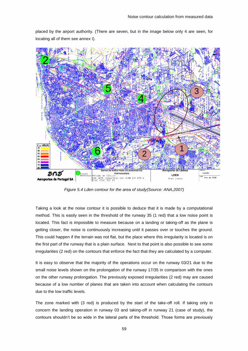
Noise contour calculation from measured data
59
placed by the airport authority. (There are seven, but in the image below only 4 are seen, for
locating all of them see annex I).
Figure 5.4 Lden contour for the area of study(Source: ANA,2007)
Taking a look at the noise contour it is possible to deduce that it is made by a computational
method. This is easily seen in the threshold of the runway 35 (1 red) that a low noise point is
located. This fact is impossible to measure because on a landing or taking-off as the plane is
getting closer, the noise is continuously increasing until it passes over or touches the ground.
This could happen if the terrain was not flat, but the place where this irregularity is located is on
the first part of the runway that is a plain surface. Next to that point is also possible to see some
irregularities (2 red) on the contours that enforce the fact that they are calculated by a computer.
It is easy to observe that the majority of the operations occur on the runway 03/21 due to the
small noise levels shown on the prolongation of the runway 17/35 in comparison with the ones
on the other runway prolongation. The previously exposed irregularities (2 red) may are caused
because of a low number of planes that are taken into account when calculating the contours
due to the low traffic levels.
The zone marked with (3 red) is produced by the start of the take-off roll. If taking only in
concern the landing operation in runway 03 and taking-off in runway 21 (case of study), the
contours shouldn‟t be so wide in the lateral parts of the threshold. Those forms are previously
1
3
2

Pablo Gauna
60
exposed on section (2.1.2). As in this study the contribution of the start of the take-off roll is not
going to be in analyzed, the resulting contours of the measures won´t have those forms besides
the threshold.
5.2 Contour calculation
The steps for this section will be:
Figure 5.5 Contour calculation process
5.2.1 Lday calculation
To calculate the Lday contour it is necessary to have the Lday calculated in each point the way
it is shown before in section (4.3.3). Once this value is calculated at all the points, they are
introduced in the Matlab program to obtain the noise surface with a linear interpolant.
The Lday for each point are the following.
Table 5.1 Lday noise values for taking-off and landing
*Measures in dB(A)
Point 1 2 3 4 5 7 8 9 10 11 12 13
Landing 58.17 65.68 67.71 65.08 57.7 64.95 61.04 64.334 59.68 55.05 61.509 73.9
Taking-Off 67.46 72.74 66.68 68.146 67.38 65.81 62.5 63.23
70.79 71.89
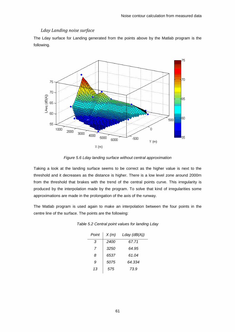
Noise contour calculation from measured data
61
Lday Landing noise surface
The Lday surface for Landing generated from the points above by the Matlab program is the
following.
Figure 5.6 Lday landing surface without central approximation
Taking a look at the landing surface seems to be correct as the higher value is next to the
threshold and it decreases as the distance is higher. There is a low level zone around 2000m
from the threshold that brakes with the trend of the central points curve. This irregularity is
produced by the interpolation made by the program. To solve that kind of irregularities some
approximations are made in the prolongation of the axis of the runway.
The Matlab program is used again to make an interpolation between the four points in the
centre line of the surface. The points are the following:
Table 5.2 Central point values for landing Lday
Point X (m) Lday (dB(A))
3 2400 67.71
7 3250 64.95
8 6537 61.04
9 5075 64.334
13 575 73.9

Pablo Gauna
62
Figure 5.7 Approximation for central values, landing Lday
This is the curve of the prolongation of the runway axis calculated from the four measured
points in the center line. The approximation given by the Matlab is the following.
Where:
Lday: Equivalent continuous sound level for one hour in day period (07:00-20:00)
x: Distance from the threshold
This equation is used to obtain more results in some points around the irregular zone (around
2000m from the threshold) and near the threshold. The new points are the following.
Table 5.3 New points´ values for Lday
Point X (m) Lday (dB(A))
1* 200 76.41
2* 800 72.72
3* 1800 68.61
4* 1900 68.31
As it is possible to see all the points are in the nearest zone to the runway, as it was said before
in that zone the changes in the noise levels are stronger that in the further zones. The necessity
of more points in those zones is another reason to make this approximation.
The resulting surface with the approximations is the following. This surface is going to be
considered the final one for Lday landing.

Noise contour calculation from measured data
63
Figure 5.8 Lday landing surface with central approximation
Lday Taking-off noise surface
The Lday surface for taking-off is calculated from the points in table 5.1 using the same
technique as in the landing surface. The taking-off surface is the following.
Figure 5.9 Lday taking-off surface
Taking a look at the taking-off surface is relevant that in the prolongation of the axis of the
runway the noise values are lower than in the outer parts. It was supposed in first instance that
could be a measurement error so some measures were repeated (Annex II, Point 4) with no
important changes from the values measured in the previous session in that same point. The

Pablo Gauna
64
lower levels in the center line can be due to the directivity of the sound on the source as it is
exposed in the “Airport planning” of the A321.
Figure 5.10 Engine noise directivity for full throttle (red line) and 21.6% throttle (blue
line)(Source: Airbus, 2011)
The points with a higher level of noise emissions are on the lateral parts of the plane, in the
center the noise is less important than besides the plane. This fact makes the take-off surface to
have the form previously exposed. It doesn´t occur when landing because, as it is possible to
see in the figure, when the engines are not at full throttle (blue line) the noise is stronger on the
front part in comparison with the sides of the plane. During the landing maneuver, as it was said
before, section (3.3.2), the airframe noise is as important as the engine noise, so the noise
surface takes the expected form shown before.
In this case is not necessary an approximation as the values in the center line have no
irregularities.
Lday noise surface
To configure the Lday surface from the previously calculated ones, it is necessary to know the
percentages of landing and taking-off of the runway over a significant period of time. In this case
that period is going to be one year. From section (4.3.2), the percent of taking-offs is 30.2% and
for landings is 69.8% for the area of study.
In each point the previously exposed noise levels (without the approximations) the values are
weighted with the percentages using

Noise contour calculation from measured data
65
Where:
Lday: Equivalent continuous sound level for one hour in day period (07:00-20:00)
LdayT_O: Lday value for take off maneuver. Table 5.1
LdayL: Lday value for land maneuver. Table 5.1
resulting the following levels.
Table 5.4 Lday noise values summary
Point Lday Land Lday Take-off Lday
1 58.17 67.46 63.3
2 65.68 72.74 69.16
3 67.71 66.68 67.42
4 65.08 68.146 66.25
5 57.7 67.38 63.14
7 64.95 65.81 65.22
8 61.04 62.5 61.53
9 64.334 63.23 64.03
12 61.509 70.79 66.63
13 73.9 71.89 73.38
These values are obtained from measures in the street where there is always a background
noise that is needed to be removed to obtain the noise contour produced by the overflying
planes. Even some care was taken when choosing the measuring points to avoid high levels of
background noise, it was inevitable to have during the day hours a noise level around 60 dB(A)
surrounding the measuring points. To take this noise out from the measure the following formula
is used:
Where:
Lday: The Lday value without background noise
Ldaym: The Lday value with background noise (from table 5.4)
Bkgr: Background noise level, 60 dB(A)
The Lday values without background noise are the following:
Table 5.5 Lday final levels
Point 1 2 3 4 5 7 8 9 12 13
Lday 60.57 68.6 66.55 65.07 60.26 63.67 56.27 61.84 65.57 73.18

Pablo Gauna
66
The surface generated with these points is the following.
Figure 5.11 Lday noise surface
5.2.2 Lnight calculation
To calculate the Lnight contour it is necessary to obtain the Lnight indicator in each point the
way shown in (4.3.3). Once those values are obtained they are introduced in the Matlab
program to calculate the noise surface with a linear interpolant. This is the same process as
with the Lday.
The Lnight for each point are the following.
Table 5.6 Lnight noise values for taking-off and landing
Lnight landing surface
As happens in the Lday landing surface it is necessary an approximation around the 2000m
from the threshold due to the program interpolation. The way to solve this problem is the same
Point 1 2 3 4 5 7 8 9 10 11 12 13
Landing 52.49 58.15 60.67 59.7 51.08 58.79 53.22 56.86 53.16 48.87 54.6 66.5
Taking-Off 63.82 68.44 58.05 59.34 59.17 57.54 54.86 56.14
64.33 63.3

Noise contour calculation from measured data
67
as in (5.2.1), introduce more points from an approximation of the central curve of the surface.
The approximation in this case is the following.
Where:
Lnight:: Equivalent continuous sound level for one hour in night period (23:00-07:00)
x: Distance from the threshold
The new introduced points are
Table 5.7 New points´ values for Lnight
Point X (m) Lnight (dB(A))
1* 200 68.58
2* 800 65.44
3* 1800 61.85
4* 1900 61.58
With these new points in the central curve the Lnight surface for landing is the following.
Figure 5.12 Lnight landing surface with central approximation
Lnight taking-off noise surface
The Lnight surface for taking-off is calculated from the points in table 5.6 using the same
technique as in the landing surface. The taking-off surface is the following.

Pablo Gauna
68
Figure 5.13 Lday taking-off surface
As it happens in the Lday taking-off surface, the central line values are lower than the ones
besides it. The reason is the same as the one exposed before in section (5.2.1).
Lnight noise surface
With the points calculated for taking-off and landing and with the percentages from section
(4.3.2), the Lnight value for each point is calculated according to the following equation.
Where:
Lnight: Equivalent continuous sound level for one hour in night period (23:00-07:00)
LnightT_O: Lnight value for take off maneuver. Table 5.6
LnightL: Lnight value for land maneuver. Table 5.6
Table 5.8 Lnight noise values summary
Point Lnight Land Lnight Take-off Lnight
1 52.49 63.82 59.30
2 58.15 68.44 64.09
3 60.67 58.05 60.03
4 59.7 59.34 59.59

Noise contour calculation from measured data
69
5 51.08 59.17 55.30
7 58.79 57.54 58.44
8 53.22 54.86 53.78
9 56.86 56.14 56.65
12 54.6 64.33 60.08
13 66.5 63.3 65.75
In this case the background noise is lower as in the night there is less activity in the streets. It is
normally around 53dB(A). Using the formula (5.4) in the same way as in section (5.2.1) the
results are the following:
Table 5.9 Lnight final values
Point 1 2 3 4 5 7 8 9 12 13
Lnight 58.14 63.73 59.072 58.52 51.44 56.99 45.96 54.2 59.13 65.51
The representation of the above values with a linear interpolant is the following.
Figure 5.14 Lnight noise surface
5.2.3 Levening calculation
For the Levening case no surfaces are going to be interpolated as they are a transition between
day and night noise levels, but not a representative contour of noise affection. The values in
each point are calculated from the “evening typical hour” the same way as the Lday and Lnight.
In this case the background noise is considered 57 dB(A).The results are the following.

Pablo Gauna
70
Table 5.10 Levening noise values summary
Point Levening Land Levening Take-off Levening Levening without
background noise
1 57.27 66.54 62.38 60.908
2 64.5 71.9 68.22 67.08
3 66.08 67.01 66.38 65.85
4 64.31 67.46 65.52 64.86
5 56.74 66.26 62.05 60.43
7 63.65 65.06 64.12 63.19
8 59.85 61.34 60.35 57.66
9 63.34 62.16 63.01 61.76
12 59.75 69.61 65.33 64.65
13 72.65 71.244 72.27 72.14
5.2.4 Lden
The Lden is the indicator that shows the global noise impact along the 24 hrs of the day. It
depends on the Lday, Levening and on the Lnight according to the formula (4.1).
Where:
Lden: The indicator that represents the noise level during all the day
Lday: LAeq,1h for hours between 07:00 and 20:00
Leve: LAeq,1h for hours between 20:00 and 23:00
Lnight: LAeq,1h for hours between 23:00 and 07:00
The Lden is going to be calculated in each point from the previously calculated Lday, Leve and
Lnight values. With the assumption that all the hours in each period are the “typical hour”, the
equation (5.7) changes to the following.
Where:
Lden: The indicator that represents the noise level during all the day
Lday: LAeq,1h for “Typical hour day”
Leve: LAeq,1h for “Typical hour evening”
Lnight: LAeq,1h for “Typical hour night”
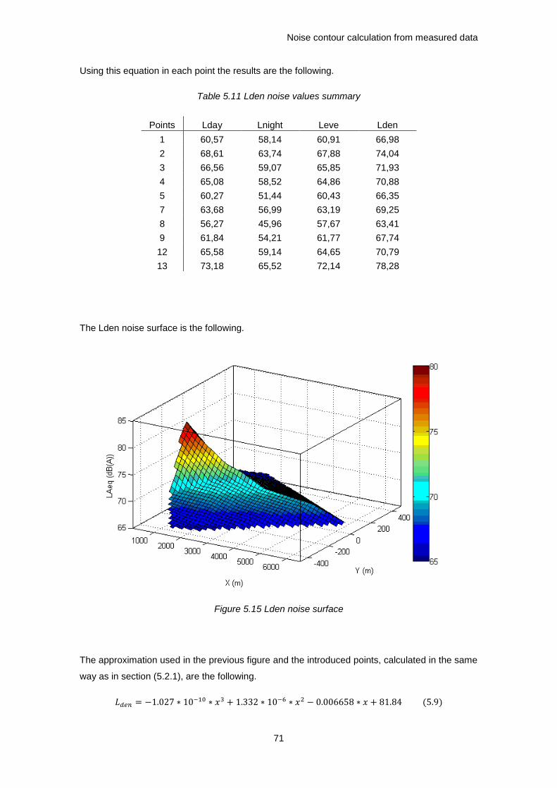
Noise contour calculation from measured data
71
Using this equation in each point the results are the following.
Table 5.11 Lden noise values summary
Points Lday Lnight Leve Lden
1 60,57 58,14 60,91 66,98
2 68,61 63,74 67,88 74,04
3 66,56 59,07 65,85 71,93
4 65,08 58,52 64,86 70,88
5 60,27 51,44 60,43 66,35
7 63,68 56,99 63,19 69,25
8 56,27 45,96 57,67 63,41
9 61,84 54,21 61,77 67,74
12 65,58 59,14 64,65 70,79
13 73,18 65,52 72,14 78,28
The Lden noise surface is the following.
Figure 5.15 Lden noise surface
The approximation used in the previous figure and the introduced points, calculated in the same
way as in section (5.2.1), are the following.

Pablo Gauna
72
Where:
Lden: Lden noise indicator
x: Distance from the threshold
Table 5.12 New points´ values for Lden
Point X (m) Lden (dB(A))
1* 200 80.56
2* 800 77.31
3* 1800 73.57
4* 1900 73.29
5.3 Contour plot
All the previously calculated surfaces have to be presented over a map of the zone affected to
show the real impact of the overflying planes. For this purpose, and with the help of the
AutoCAD program, the surfaces are presented over a map of the city of Libon. The results are
the following noise contours.
Figure 5.16 Lden measured noise contour

Noise contour calculation from measured data
73

Pablo Gauna
74
6. Conclusions & proposal for future study
6.1 “Multiple threshold” noise reduction proposal for further study
As it was shown in section (4.3.2) the majority of the time the area of study is affected by planes
in landing maneuver. This maneuver follows a straight line that starts on the threshold with 3º of
inclination until the FAP (5.1.2), all the planes over the same line.
Smaller planes need shorter distances for taking-off and for landing. The actual runways are
designed for the bigger plane able to operate into them, so for the smaller planes the runway is
bigger than the length they need.
A “multiple thresholds” technique is proposed as a measure to separate from the ground as
much as possible the planes that don‟t need the whole runway to operate by creating another
threshold only usable by those “little” planes. The proposed displacement for the case in study
is of 1200 m.
Figure 6.1 Possible two different landing flight tracks
Taking a look at the traffic in Lisbon, the bigger C type plane (that represents the 67.32% of the
whole traffic) is the A321 which needs a distance about 2000 meters for landing in the worst of
the cases according to its airport planning [29]. Supposing that the rest of the C and the G type
planes, as they are smaller, they can land in that distance, about the 68.32% of the traffic would
be into this measure, leaving the A340 and the D type planes operating with the actual runway
length. Placing the “secondary” threshold at 1200 meters from the actual, the “short” runway
would be of 2605 meters, even bigger than the runway 17/35 (2304 meters) in which C type
planes operate.

Noise contour calculation from measured data
75
Figure 6.2 Possible displaced threshold (Source: Google maps)
The displacement of 1200m means that planes overfly 62.8 meters higher the city so a
reduction of noise should be produced over the populated areas in study in this document. The
new noise contour is the same calculated before but displaced a distance near to 1200m (the D
and E type planes continue making the same noise as before).
Figure 6.3 Comparative between noise under selective threshold
Some technical difficulties must be studied to check the availability of this measure. There
should be different lights for both operations of the runway (shot and long), and the ILS has to
be studied in deep so as to know if it is possible to have two different Glide Paths with one
Localizer. Also the controllers and pilots must learn to operate with two thresholds in the same
runway.
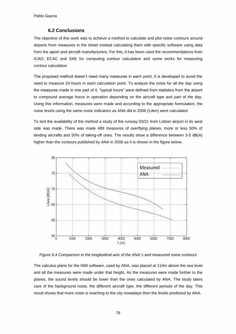
Pablo Gauna
76
6.2 Conclusions
The objective of this work was to achieve a method to calculate and plot noise contours around
airports from measures in the street instead calculating them with specific software using data
from the aiport and aircraft manufacturers. For this, it has been used the recommendations from
ICAO, ECAC and SAE for computing contour calculation and some works for measuring
contour calculation.
The proposed method doesn‟t need many measures in each point, it is developed to avoid the
need to measure 24 hours in each calculation point. To analyze the noise for all the day using
the measures made in one part of it, “typical hours” were defined from statistics from the airport
to compound average hours in operation depending on the aircraft type and part of the day.
Using this information, measures were made and according to the appropriate formulation, the
noise levels using the same noise indicators as ANA did in 2006 (Lden) were calculated.
To test the availability of the method a study of the runway 03/21 from Lisbon airport in its west
side was made. There was made 489 measures of overflying planes, more or less 50% of
landing aircrafts and 50% of taking-off ones. The results show a difference between 3-5 dB(A)
higher than the contours published by ANA in 2006 as it is shown in the figure below.
Figure 6.4 Comparison in the longitudinal axis of the ANA´s and measured noise contours
The calculus plane for the INM software, used by ANA, was placed at 114m above the sea level
and all the measures were made under that height. As the measures were made further to the
planes, the sound levels should be lower than the ones calculated by ANA. The study takes
care of the background noise, the different aircraft type, the different periods of the day. This
result shows that more noise is reaching to the city nowadays then the levels predicted by ANA.

Noise contour calculation from measured data
77
The problem of noise in Lisbon is not in near or easy solution. The fact of being in the middle of
the city obliges the planes to flyover it and disturb the people living or working there. As it was
shown in section (5.1.1) there is a big list of noise measures implemented to reduce that
affection to the surrounding areas of the airport.
The proposal of selective thresholds shows a reduction between four to one dB(A) in the noise
affection to the city. The implementation of this technique is not complex because there is not
new technology involved and the landing procedures stay nearly the same. The difficulty is to
develop it and teach the personal how to work in that new procedure situation.

Pablo Gauna
78
Bibliography
[1] FAA, Federal Aviation Administration, (1985); “Aviation noise effects”, March 1985.
ADA-154319
[2] BENITO, A. “Impacto ambiental del transporte aereo, Tipos de impactos ambientales”,
2009
[3] HEATHROW AIPORT (2009); “Environmental noise directive, Noise action plan 2010-
2015”, November 2009
[4] ICAO, Intenational Civil Aviation Organization, (1987); “Recommended Method for
Computing Contours around Airports”; Circ. 205-AN/1/25; 11 March 1987
[5] ECAC, European Civil Aviation Conference, (2007); “Report on standard method of
computing noise contours around civil airports”, Doc.29, 2nd
Edition, July 1997
[6] SAE, Society of Automobile Engineers, (1986); “Procedure for the Calculation of
Airplane Noise in the Vicinity of the Airports”, SAE_AIR_1845; March, 1986
[7] ICAO, International Civil Aviation Organization, (2008); “Guidance on the Balanced
Approach to aircraft noise management”, Doc.9829; AN/451; Second Edition; 2008
[8] SCHIPHOL AIRPORT:
http://www.schiphol.nl/SchipholGroup/CorporateResponsibility/EnvironmentAndNoise/N
oiseAndDisturbanceReduction.htm (15 December, 2011)
[9] SEATTLE-TACOMA AIRPORT: http://www32.webtrak-lochard.com/WebTrack/sea (15
December, 2011)
[10] ICAO, International Civil Aviation Organization, (2009); “Politicas de la OACI sobre
derechos aeroportuarios y por servicios de navegacion aerrea”, Doc. 9082, Octava
Edicion, 2009
[11] OLLERHEAD, J. B. “The CAA Aircraft Noise Contour Model: ANCON Version1”; DORA
report 9120, November 1992
[12] JOPSON, I; DR. RHODES, D; HAVELOCK, P; “Aircraft Noise model validation- How
accurate do we need to be?”; CAA Environmental Research and Consultancy
Department, Kingsway, London
[13] ASENSIO, C; PAVON, I; RUIZ, M; PAGAN, R; RECUERDO, M; “Estimation of
directivity and sound Power levels emitted by aircrafts during taxiing, for outdoor noise
prediction purpose”; Applied Acoustics, Volume 68, Issue 10, Octover 2007, 1263-1279

Noise contour calculation from measured data
79
[14] CLEMENTE, J; GAJA, E; CLEMENTE, G; REIG, A; “Sensitivity of the FAA Integrated
Noise Model to input parameters”; Applied Acoustics, Volume 66, Issue 3, March 2005,
263-276
[15] ASENSIO, C; PAVON, I; RUIZ, M; PAGAN, R; RECUERDO, M; “Aircrafts´ taxi noise.
Sound power level and directivity frequency band results”; Applied Acoustics, Volume
70, Issue 7, July 2009, 986-1008
[16] DAESEUNG CHO; JIN HYEONG KIM; DOUGLAS MANVELL; Noise mapping using
measured noise and GPS data”; Applied Acoustics, Volume 68, Issue 9, September
2007, 1054-1061
[17] STANSFELD, S.A, MATHERSON, M.P; “Noise pollution: non-auditory effects on
health”; British Medical Bulletin 2003; 68; 243-257
[18] COELHO, J.L.B, FERREIRA A.J; “Critérios para análise de relações exposição-impacte
do ruído de infra-estruturas de transporte”; Grupo de acústica e controlo do ruído do
Centro de Análise e Processamento de Sinais (CAPS); December 2009
[19] PUIG, S.J; “Audio digital y MIDI, Guias Monograficas”; Anaya Multimedia, Madrid 1997
[20] ANA,Aeroportos de Portugal; “Aeroporto de Lisboa, Mapa de ruido, Resumo não
técnico”; Março 2007
[21] MAXIM Integrated products; “Quantitative Analysis Yields Objective Measurement for
Audio Amplifier Click and Pop”; Application note 3687; November 29, 2005
[22] ZAPOROZHETS, O.I; TOKAREV, V. I; “Aircraft noise modeling for environmental
assessment around airports”; Applied Acoustics, Volume 55, Issue 2, Octover 1998, 99-
127
[23] OLLERHEAD, J. B. “The CAA Aircraft Noise Contour Model: ANCON Version1”; DORA
report 9120, November 1992
[24] STANSTED AIRPORT (2006); “ANCON Version 2 Model Overview”; Appendix A5; April
2006
[25] ICAO, International Civil Aviation Organization (2008); “Environmental protection;
Volume 1; Aircraft noise” Annex 16 to the Convention on International Civil Aviation,
Fifth Edition, July 2008
[26] AIRBUS INDUSTRIES (2003); “Getting grips with aircraft noise” Flight Operations
Support & Line Assistance; Blagnac, France; December 2003
[27] EUROPEAN UNION. Directiva 2002/30/CE del Parlamento Europeo y del Consejo
sobre el establecimiento de normas y procedimientos para la introducción de
restricciones operatives relacionadas con el ruido en los aeropuertos comunitarios.
March, 26th 2002
[28] ICAO, International Civil Aviation Organization (2004); “Aerodromes desing and
aerodromes operation”; Annex 14 to the Convention on International Civil Aviation,
Fourth Edition, July 2004
[29] AIRBUS INDUSTRIES. Airplane characteristics for Airport Planning for A318, A319,
A320, A321, A330, A300, A310, A340

Pablo Gauna
80
[30] BOEING CO. Airplane characteristics for Airport Planning for B737, B767, B757, B777,
MD80,MD90.
[31] EMBRAER. Airplane characteristics for Airport Planning for E134, E140, E145, E170,
E190, E195.
[32] Decreto-Lei n. 146/2006. Ministério do ambiente, do ordenamento do territorio e do
desenvolvimento regional. 31 July, 2006
[33] ANA, Aeroportos de Portugal (2010); Relatorio anual de estadísticas de tráfego 2009
[34] ANA, Aeroportos de Portugal (2006); Plano de expansão de aeroporto de Lisboa.
November 2006
[35] NAV Portugal (2004), “Noise abatement procedure”; E.P.E. AIC A 012-2004,. July
2004.
[36] AIP Portugal (2011). Standard departure chart- instrument for runway 21. June 2011
[37] AIP Portuga (2011)l. Instrument Approach Chart for runway 03. March 2011
[38] AIP Portugal (2011). Aircraft parking/ Docking chart. June 2011
[39] MINISTÉRIO DO AMBIENTE, DO ORDENAMENTO DO TERRITÓRIO E DO
DESENVOLVIMENTO REGIONAL. Decreto-Lei n.º 9/2007. January 2007
Noise contour calculation from measured data
81
Annex I
ANA´s Noise contours

Pablo Gauna
82

Noise contour calculation from measured data
83

Pablo Gauna
84

Noise contour calculation from measured data
85
Annex II
Measures

Pablo Gauna
86
Point 1
Take off (14/11/2011) Land (15/11/2011)
TIME COMPANY TYPE SEL TIME COMPANY TYPE SEL
1015 TAAG D 93,8 1445 TAP C 83,3
1020 TAP340 E 97 1448 AF C 84,9
1025 TAP C 95,9 1452 KLM C 83,8
1042 TAP MD G 92,7 1458 TAP C 83,7
1049 TAP D 95,4 1502 TAP C 82,7
1055 AF C 91,5 1505 AE C 84,8
1059 Conti D 92,4 1522 TAP C 82,7
1137 - Priv 83,5 1546 TAP 340 84,7
1139 - G 90,7 1550 TAP C 85,2
1202 TAP C 90,9 1603 Luft C 83,2
1220 Luft C 93,8 1909 TAP C 82,2
1226 White D 91,7 1611 TAP C 82
1229 Luft C 90,6 1614 TAP G 78,1
1231 Swiss C 96,8 1638 TAP C 84,3
1247 TAP C 91,8 1645 EASY C 83
1305 TAP C 93 1647 TAP D 84,4
1307 TAP C 91,8 1728 AF C 82,6
1312 - Priv 92 1731 EASY C 82,6
1319 Ib C 91,8 1329 GermanW C 90,5 1335 TAP MD G 87 1347 AF G 83,1 1354 SATA D 96,3

Noise contour calculation from measured data
87
Point 2
Take off (09/12/2011) Land (15/11/2011)
TIME COMPANY TYPE SEL TIME COMPANY TYPE SEL
1438 TAP C 96,7 1134 Luft C 91,2
1442 TAP G 91,8 1150 TAP C 92,3
1446 Swiss C 98,4 1203 TAP D 94,7
1454 Luft C 101 1207 EASY C 90,2
1457 TAP C 97,6 1211 Blanco C 90,1
1501 TAP C 98,3 1214 SATA C 90,5
1506 TAP C 96,9 1216 TAP G 85
1509 TAP G 91,5 1220 TAP G 85,2
1515 EASY C 98,1 1236 TAP G 85,7
1520 TAP C 97,6 1240 Brusels C 92,4
1522 Priv AB 92,4 1243 TAP G 86,2
1524 TAP C 95,5 1247 Ib C 91,1
1526 TAP C 97,3 1252 AF reg C 85,8
1528 EASY C 97 1259 Luft C 91,1
1534 TAP G 90,8 1300 TAP G 85,4
1536 TAP C 101 1304 TAP C 88,9
1541 TAP C 97,3 1315 Swiss C 91,4
1544 TAP C 97 1319 EASY C 91,6
1549 TAP C 95,5 1321 TAP C 91
1557 AE C 97,3 1322 TAP G 86,3
1606 TAP C 94,7 1326 TAP C 90,4
1608 KLM C 100,5 1329 TAP C 91
1612 TAP C 95,6 1331 Euroatlantic D 94,6
1617 SATA D 99,4 1335 TAP C 91,7
1344 TAP C 90,4
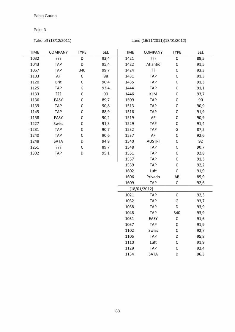
Pablo Gauna
88
Point 3
Take off (13/12/2011) Land (16/11/2011)(18/01/2012)
TIME COMPANY TYPE SEL TIME COMPANY TYPE SEL
1032 ??? D 93,4 1421 ??? C 89,5
1043 TAP D 95,4 1422 Atlantic C 91,5
1057 TAP 340 99,7 1424 ?? C 93,3
1103 AF C 88 1431 TAP C 91,3
1120 Brit C 90,4 1435 TAP C 91,3
1125 TAP G 93,4 1444 TAP C 91,1
1133 ??? C 90 1446 KLM C 93,7
1136 EASY C 89,7 1509 TAP C 90
1139 TAP C 90,8 1513 TAP C 90,9
1145 TAP C 88,9 1516 TAP C 91,9
1158 EASY C 90,2 1519 AE C 90,9
1227 Swiss C 91,3 1529 TAP C 91,4
1231 TAP C 90,7 1532 TAP G 87,2
1240 TAP C 90,6 1537 AF C 92,6
1248 SATA D 94,8 1540 AUSTRI C 92
1251 ??? C 89,7 1548 TAP C 90,7
1302 TAP D 95,1 1551 TAP C 92,8
1557 TAP C 91,3
1559 TAP C 92,2
1602 Luft C 91,9
1606 Privado AB 85,9
1609 TAP C 92,6
(18/01/2012)
1021 TAP C 92,3
1032 TAP G 93,7
1038 TAP D 93,9
1048 TAP 340 93,9
1051 EASY C 91,6
1057 TAP C 91,9
1102 Swiss C 92,7
1105 TAP D 95,8
1110 Luft C 91,9
1129 TAP C 92,4
1134 SATA D 96,3

Noise contour calculation from measured data
89
Point 4
Take off (12/12/2011) (18/01/2012) Land (17/11/2011)
TIME COMPANY TYPE SEL TIME COMPANY TYPE SEL
1453 TAP C 90,6 1552 Luft C 91,1
1457 Luft C 92,3 1554 Ib C 91,5
1500 TAP C 88,7 1556 TAP C 90,8
1503 EASY C 91,5 1601 TAP C 88,5
1508 TAP G 88 1644 EASY C 89,5
1510 TAP C 91,8 1701 TAP C 91,2
1512 TAP C 92,1 1714 EASY C 90,9
1514 TAP C 92,6 1721 TAP C 89,9
1517 TAP C 92 1731 AF C 90,1
1526 TAP C 89,7 1739 TAP D 93,2
1533 TAP C 93,3 1741 EASY C 89,4
1539 TAP G 86,7 1750 TAP G 84,7
1557 TAP D 94,2 1753 STAR C 91,8
1600 ???? C 92 1756 TAP C 90
1604 TAP D 99,2 1759 Privado B 88,3
1611 TAP C 91,2 1801 TAP C 89
1613 ???? C 93,6 1804 TAP C 92,9
1615 TAP D 96,6 1806 Brit C 90
1619 TAP C 91 1809 Blanco C 91,5
1621 TAP C 90,9 1814 EASY C 91,1
(18/01/2012)
1816 EASY C 90
1416 TAP C 93 1820 TAP G 86,7
1421 TAP G 93,4 1824 Lingus C 91,3
1429 TAP G 86,6 1831 TAP C 90,5
1430 TAP C 91,4 1436 TAP C 91,7 1440 Luft C 92,3 1444 TAP C 90,5 1450 TAP C 90,3 1500 TAP C 93,2 1503 ??? C 91,6
*The measure repeated on take-off maneuver the 18th of January was made with the intention of
checking if the non expected contour for take of came from a wrong measure. The results are
similar to the ones measured the 12th of December, so it wasn´t a problem in the measure.

Pablo Gauna
90
Point 5
Take off (18/12/2011) Land (18/11/2011)
TIME COMPANY TYPE SEL TIME COMPANY TYPE SEL
1227 Luft C 91,2 1037 STAR D 85,2
1231 Swiss C 92,1 1045 TAP C 82,1
1244 TAP C 93,6 1050 TAP C 82,5
1247 Luft C 89,5 1100 EASY C 82,4
1250 TAP D 95,6 1102 EASY C 82,5
1259 ???? C 93 1105 TAP D 85,1
1302 SATA D 96 1107 TAP G 79,3
1307 TAP G 92,6 1114 TAP D 88,7
1310 Ib C 91,2 1117 TAP C 83,6
1313 ??? C 92,2 1128 Luft C 84,6
1319 Brusels C 94,4 1134 TAP D 86,5
1321 TAP G 84,4 1137 Luft C 83,6
1324 ??? C 91,4 1140 TAP C 83,1
1345 TAP 340 96,1 1142 Swiss C 85
1350 TAP C 92,5 1151 TAP G 78,6
1352 TAP C 93,6 1154 TAP 340 84,3
1355 EASY C 91,1 1157 TAP G 79,1
1200 TAP C 83,2
1203 Brusels C 84,2
1205 Ib C 81,4

Noise contour calculation from measured data
91
Point 7
Take off (16/12/2011) Land (21/11/2011)
TIME COMPANY TYPE SEL TIME COMPANY TYPE SEL
1342 TAP D 92,4 1410 TAP C 89,4
1345 Priv AB 86,3 1411 TAP C 89,6
1358 TAP G 95,5 1419 STAR D 92,7
1410 TAP C 89,3 1424 TAP C 90,7
1416 German C 88 1427 Priv AB 85,1
1420 TAP C 89,4 1429 TAP C 90,9
1425 ??? C 90,7 1431 TAP C 88,2
1437 TAP C 88,5 1445 TAP C 91,2
1441 TAP G 83,7 1450 TAP C 91
1444 AF G 82,8 1452 TAP G 85,1
1453 TAP C 89,4 1455 STAR C 89
1455 Luft C 91,2 1507 TAP C 87,9
1504 Swiss C 87,7 1530 TAP C 88,4
1507 TAP C 90,7 1538 AE C 90,2
1517 TAP C 88,3 1543 AirBerlin C 91,5
1522 Easy C 87,2 1545 ??? C 89,3
1526 TAP C 88,7 1549 AE C 90,1
1529 TAP C 89,6 1551 TAP C 88,8
1531 TAP C 90,2 1555 TAP C 88,4
1540 EASY C 89,2 1558 Luft C 89,4
1601 KLM C 92,2
1604 TAP 340 90,9

Pablo Gauna
92
Point 8
Take off (15/12/2011) Land (23/11/2011)
TIME COMPANY TYPE SEL TIME COMPANY TYPE SEL
1148 TAP G 86,6 1120 Luft C 88,3
1202 TAP C 88,5 1129 SATA D 90
1208 TAP C 87,8 1131 TAP C 87,9
1212 EASY C 86,6 1139 Ib C 86,3
1230 Swiss C 88,1 1156 TAP D 91,9
1235 Luft C 87,4 1200 TAP C 87,3
1242 TAP C 87,4 1202 TAP G 84,6
1248 TAP D 92,5 1206 Brussels C 86,4
1251 TAP 340 94 1210 TAP D 92
1256 TAP C 86,2 1213 TAP C 87,1
1313 TAP G 79,7 1216 German C 84,9
1315 TAP C 81,5 1221 Easy C 86,5
1317 Brussels C 84,8 1224 TAP G 83,9
1340 German C 85,1 1238 TAP G 82
1348 EASY C 86,4 1249 TAP C 88,5
1350 TAP C 87 1300 TAP G 84,3
1355 TAP G 79,5 1309 TAP C 86,6
1413 TAP G 86,1 1315 TAP C 85,7
1419 EASY C 87,5 1317 TAP G 81,3
1424 TAP C 86 1321 TAP C 87,4
1324 TAP C 86,8
1327 TAP C 85,6
1339 Luft C 86,7
1348 TAP C 85,3
1352 TAP D 88,4
1354 TAP C 87,2
1356 TAP C 87

Noise contour calculation from measured data
93
Point 9
Take off (15/12/2011) Land (23/11/2011)
TIME COMPANY TYPE SEL TIME COMPANY TYPE SEL
1508 TAP C 86,8 1155 Luft C 88,7
1510 TAP G 85,1 1203 Brussels C 90,3
1513 TAP C 88,7 1206 TAP G 86,3
1519 TAP C 89,7 1209 TAP C 89,3
1523 ??? C 87,4 1228 Easy C 89,4
1536 TAP G 82,3 1231 TAP G 87,4
1548 KLM C 89,6 1246 Swiss C 89,8
1558 KLM C 87,6 1248 ?¿? G 84,2
1600 TAP C 88,5 1252 German C 88,2
1607 TAP C 86,4 1255 Luft C 91,6
1609 TAP D 91,6 1301 TAP C 88,3
1616 TAP D 88,1 1308 TAP C 90,3
1618 TAP D 91,6 1313 TAP C 89,7
1626 ??? C 86,6 1315 TAP C 88,9
1627 TAP C 86,4 1323 ?¿? D 94,1
1633 TAP C 88,7 1329 TAP C 89,9
1650 TAP G 88,1 1332 TAP C 89,5
1652 TAP D 91,1 1335 TAP C 90,7
1654 TAP D 92,9 1339 TAP C 90,3
1701 TAP D 91,6 1342 TAP G 85,1
1704 ??? C 88 1345 TAP G 84,8
1349 TAP C 90,7

Pablo Gauna
94
Point 10 Point 11
Land (25/11/2011) Land (25/11/2011)
TIME COMPANY TYPE SEL
1433 TAP C 84,8
1436 TAP C 88,5
1451 TAP C 85,4
1455 TAP G 79,9
1459 TAP C 83,9
1507 TAP C 86
1520 TAP G 80,4
1524 AE C 85,2
1527 TAP C 84,6
1529 AF C 86,6
1532 TAP C 83,5
1537 AirBerlin C 89
1553 TAP C 85,5
1558 TAP C 85,4
1600 TAP C 85,4
1607 Agroar C 86,3
1615 TAP D 81,5
1623 Luft C 84,3
1651 Ib C 86
1716 SATA D 87,6
TIME COMPANY TYPE SEL
1802 Brit C 79,2
1814 AerLingus C 80,9
1819 TAP 340 82,1
1822 Easy C 80,8
1826 TAP C 80,9
1828 TAP C 81,9
1831 Easy C 80,9
1833 TAP G 77,1
1836 TAP C 82,1
1839 ¿?¿ C 80,5
1842 TAP C 81,6
1845 TAP C 80,7
1848 TAP G 75,9
1852 TAP C 81
1855 Easy C 81,1
1857 Easy C 81,8
1901 TAP C 81,2
1903 AE C 82
1918 ¿?¿ D 82,3
1946 TAP G 76,5

Noise contour calculation from measured data
95
Point 12
Take off (12/12/2011) Land (19/12/2011)
TIME COMPANY TYPE SEL TIME COMPANY TYPE SEL
1230 Luft C 92,5 1127 Luft C 86,7
1233 Swiss C 98,5 1129 Swiss C 88,4
1235 TAP C 94,3 1132 TAP C 84,5
1238 Priv AB 85,3 1136 TAP D 89,5
1246 IB C 93,8 1147 SATA C 86
1249 SATA D 100,7 1206 TAP C 84,4
1254 EASY C 94,1 1208 Swiss C 89,3
1302 Priv AB 84,7 1216 TAP G 79,5
1305 TAP C 92,7 1224 Brus C 86,9
1311 TAP C 94,5 1229 EASY C 85,4
1317 TAP G 87,4 1236 German C 84,3
1319 GermanW C 93,8 1249 TAP C 85,5
1323 ??? C 98,8 1306 TAP C 84,4
1340 EASY C 92,1 1310 AF G 78,9
1345 TAP C 95,7 1314 TAP G 81,8
1348 SATA D 98 1320 TAP C 86,5
1351 AF C 87,3 1334 TAP G 80,3
1353 TAP C 94,5 1345 TAP G 82,2
1400 TAP C 94 1347 TAP C 84,2
1402 TAP C 93,7 1350 TAP G 80,5
1352 TAP D 87,4
1356 TAP C 84,9

Pablo Gauna
96
Point 13
Take off (12/12/2011) Land (19/12/2011)
TIME COMPANY TYOE SEL TIME COMPANY TYPE SEL
1558 TAP C 96,3 1029 TAP C 96,8
1603 TAP D 102,8 1033 Priv AB 96,5
1606 TAP C 96,7 1044 TAP C 98,8
1608 KLM C 94,8 1046 TAP C 97,4
1610 TAP C 92,9 1051 TAP G 93,9
1611 TAP G 92 1054 EASY C 98
1618 AE C 95,3 1056 TAP D 99,7
1620 TAP C 93,6 1059 TAP D 100,5
1621 ??? C 94,3 1114 ??? C 100,7
1630 TAP C 94 1121 Luft C 99,3
1639 TAP D 101 1126 TAP C 97,7
1644 TAP D 101 1129 EASY C 99
1649 TAP C 93,7 1132 TAP D 102,1
1653 IB C 91 1136 TAP D 102,4
1655 TAP D 100,6 1140 Luft C 98
1657 TAP D 101,1 1142 TAP D 100,9
1659 Luft C 97,6 1144 SATA C 98,3
1720 TAP G 95,2 1146 IB C 99,7
1730 EASY C 95,8 1149 TAP C 99,3
1735 EASY C 97,8 1159 TAP G 92,7
1744 TAP G 88,5

Noise contour calculation from measured data
97
Annex III
2009 ANA Statistics

Pablo Gauna
98

Noise contour calculation from measured data
99