energy use in the australian residential sector 1986-2020 ... · energy use in the australian...
TRANSCRIPT

ENERGY USE IN THE AUSTRALIAN RESIDENTIAL SECTOR
1986 – 2020

ii
ENERGY USE IN THE AUSTRALIAN RESIDENTIAL SECTOR
Published by the Department of the Environment, Water, Heritage and the Arts
© Commonwealth of Australia 2008
ISBN: 978-1-921298-14-1
This work is copyright. It may be reproduced in whole or part for study or training purposes, subject to the inclusion of an acknowledgement of the source and no commercial usage or sale. Reproduction for purposes other than those listed above requires the written permission from the Department of the Environment, Water, Heritage and the Arts (DEWHA). Requests and enquiries concerning reproduction and rights should be addressed to:
The Communications Director Department of the Environment, Water, Heritage and the Arts GPO Box 787 Canberra ACT 2601
This report was prepared by Energy Efficient Strategies for DEWHA. The views and opinions expressed in this publication are those of the authors and do not necessarily reflect those of the Australian Government or the Minister for the Environment, Water, Heritage and the Arts.
While reasonable efforts have been made to ensure that the contents of this publication are factually correct, the Commonwealth does not accept responsibility for the accuracy or completeness of the contents, and shall not be liable for any loss or damage that may be occasioned directly or indirectly through the use of, or reliance on, the contents of this publication.
Design: Giraffe Visual Communication Management
Main cover photo: Emma Cross All other photos courtesy of www.yourhome.gov.au unless otherwise referenced.

iii
CONTENTS
Executive Summary ix
Main findings ix
Trends by fuel type ix
Trends by end use ix
Trends in building shell efficiency x
Emerging trends x
Areas for further research xii
1 Introduction 2
1.1 Background 2
1.2 Scope of work 2
1.3 Project team and acknowledgements 3
2 Project overview 6
2.1 Project approach 6
2.2 Modelling overview 6
2.3 Appliance modelling methodology 7
2.4 Tracking appliance end uses 10
2.5 Housing stock modelling methodology 11
2.6 Space conditioning load modelling methodology 12
2.7 Areas identified for further research 13
3 Key results and trend analysis 20
3.1 Introduction 20
3.2 The national perspective 20
3.3 Breakdown by state 30
3.4 Appliances 40
3.5 Cooking 40
3.6 Water heating 40
3.7 Space conditioning 40
4 Results by end use 48
4.1 Overview 48
4.2 Space cooling equipment 48
4.3 Space heating equipment 49
4.4 Water heating 50
4.5 Cooking products 51
4.6 Major appliances 53
4.7 Information technology products 55
4.8 Home entertainment equipment 57
4.9 Other equipment 62

ENERGY USE IN THE AUSTRALIAN RESIDENTIAL SECTOR
iv
5 Population and household estimates 70
5.1 Overview of estimates 70
5.2 Estimates used for this study 70
6 Appliance modelling methodology 74
6.1 Overview 74
6.2 Attributes 74
6.3 User interaction with products 75
6.4 Climate and weather 77
6.5 Ownership and stock of appliances 79
6.6 Input assumptions by product type 82
7 Housing stock modelling methodology 100
7.1 Overview 100
7.2 Stock characteristics / categorisation 101
7.3 Base year estimates – 1986 103
7.4 Model inputs (Post -1986) 111
7.5 Adjustments to estimates of housing numbers 118
7.6 Floor area estimates 119
7.7 Division into climate zones 124
8 Space conditioning load modelling methodology 140
8.1 Overview 140
8.2 Modelling tools 140
8.3 Sample housing 141
8.4 Occupancy profiling 142
8.5 Zoning 145
8.6 Thermostat operation 149
8.7 Climate files 152
8.8 Miscellaneous settings and assumptions 155
9 Calibration of the stock model 160
9.1 Process overview 160
9.2 Overview of state total energy consumption – top-down vs bottom-up 161
10 Data sources and references 164
10.1 Overview of data sources 164
10.2 References 165

CONTENTS
v
Appendix A – Comparison of EES model outputs against top-down data sources 171
A.1 Overview 171
A.2 Australia 171
A.3 NSW and ACT 174
A.4 Victoria 177
A.5 Queensland 179
A.6 South Australia 179
A.7 Western Australia 181
A.8 Tasmania 181
A.9 Northern Territory 183
Appendix B – Air conditioner sub-model 185
B.1 Overview 185
B.2 Key air conditioner attributes 185
Appendix C – Refrigerator and freezer sub-model 189
C.1 Overview 189
C.2 Key refrigerator attributes that impact on energy consumption 189
Appendix D – Solar water heater performance attributes 195
D.1 Overview 195
D.2 Key solar water heater attributes 196
List of Tables 201
List of Figures 206

ENERGY USE IN THE AUSTRALIAN RESIDENTIAL SECTOR
vi
Appendices E – H can be found on the CD inside the back Cover
Appendix E – Model inputs - attributes 213
Appendix F – Model inputs - ownership 255
Appendix G – Model outputs 347
Appendix H – Model inputs - Housing stock details 371
All States 371
NSW 375
VIC 397
QLD 439
SA 441
WA 467
TAS 489
NT 511
ACT 533
Abbreviations – General
ABARE Australian Bureau of Agricultural and Resource Economics
ABS Australian Bureau of Statistics
AC Air conditioner
AGA Australian Gas Association
AGO Australian Greenhouse Office
BOM Bureau of Meteorology, Australia
CBA Cost Benefit Analysis
DEWHA Department of the Environment, Water, Heritage and the Arts
E3 Equipment Energy Efficiency Committee
EES Energy Efficient Strategies P/L
ERP Estimated Resident Population
ESAA Energy Supply Association of Australia
ETSA Electricity Trust of South Australia
HIA Housing Industry Association of Australia
MEPS Minimum Energy Performance Standards
NAEEEC National Appliance and Equipment Energy Efficiency Committee (now E3)
NatHERS Nationwide House Energy Rating Scheme
NEMMCO National Electricity Market Management Company
NGGI National Greenhouse Gas Inventory
NIEIR National Institute For Economic and Industrial Research
RIS Regulatory Impact Study
SEAV Sustainable Energy Authority of Victoria – formerly EEV (now Sustainability Victoria)

CONTENTS
vii
TMY Typical Meteorological Year
REC Renewable Energy Certificate
ORER Office of Renewable Energy Regulator
Abbreviations – Charts
The following abbreviations are used in this report to include a range of appliance types
Electrical Equipment
CD Clothes dryers (rotary electric)
CFLs Compact Fluorescent lights
CW front Clothes washers – front loading (drum) (horizontal axis)
CW top Clothes washers – top loading (agitator and impeller) (vertical axis)
DVD DVD (includes players and recorders, some with hard disk)
DW Dishwashers
FZ Freezers (separate – composite includes vertical and chest types)
Games Games consoles
Home ent. Home entertainment other (mostly other audio equipment)
Kettles Electric kettles (jugs) to boil water
Laptops Computers – laptop
Lighting Lighting (composite total lighting end use for the whole house)
Microwave Microwaves (separate) (conventional and convection combination)
Misc. ITS Miscellaneous IT equipment switched (printers, speakers)
Misc. ITU Miscellaneous IT equipment un-switched (other IT items)
Miscell. Other electricity (small miscellaneous loads, some secondary heating)
Monitors Monitors (used with desktop computers) (CRT and LCD type)
Other Sby Other standby (other products not already explicitly covered)
PC Computers – desktop (box only)
Pools Swimming pools – electricity / gas (includes pumps and heating)
RF Refrigerators (composite includes single door refrigerator-freezers)
Spas Spas – electricity / gas (includes pumps and heating)
STB FTA Set Top Box – free to air digital (simple converter boxes or DTAS)
STB PAY Set Top Box – subscription (pay TV – cable, microwave or satellite)
TV Television – composite of CRT, LCD, Plasma and Projection technologies
VCR Video Cassette Recorder (VCR) (includes combo DVD players)
Cooking Equipment (all items may be separate or part of a “range”)
Cook El Cooking – electric cook-top
Cook gas Cooking – mains gas cook-top
Cook LPG Cooking – LPG cook-top
Oven El Cooking – electric oven (separate or part of a range)
Oven gas Cooking – mains gas oven (separate or part of a range)
Oven LPG Cooking – LPG oven (separate or part of a range)

ENERGY USE IN THE AUSTRALIAN RESIDENTIAL SECTOR
viii
Water Heating Equipment
Electric Electric storage
Gas Inst Gas instantaneous (mains gas) (no storage)
Gas Stor Gas storage (mains gas)
LPG Inst Gas instantaneous (LPG)
LPG Stor Gas storage (LPG)
Solar El A Solar electric (flat plate thermal) – solar contribution
Solar El B Solar electric (flat plate thermal) – external boost fuel
Solar GI A Solar gas in line instantaneous boost – solar contribution
Solar GI B Solar gas in line instantaneous boost – external boost fuel
Solar GS A Solar gas in tank boost – solar contribution
Solar GS B Solar gas in tank boost – external boost fuel
Solar HP A Heat pump – solar contribution
Solar HP B Heat pump – external fuel
Space Conditioning Equipment
DuctC Cooling – AC ducted (composite cooling only and reverse cycle types)
Ductgas Heating – mains gas ducted
DuctRCH Heating – AC reverse-cycle ducted
El Resist Heating – electric resistive (mostly portable units run from GPOs)
Evap Cooling – evaporative (mostly central)
RCOC Cooling – AC cooling only non-ducted (split and window wall)
Room Gas Heating – mains gas non-ducted (room heater)
RoomLPG Heating – LPG gas non-ducted (room heater)
RRCC Cooling – AC reverse non-ducted (composite split and window wall)
RRCH Heating – AC reverse-cycle non-ducted
Wood C Heating – wood – closed combustion
Wood O Heating – wood – open combustion
Note: Mains gas is reticulated natural gas (mostly methane) in most cases.

ix
EXECUTIVE SUMMARY
EXECUTIVE SUMMARY
Climate change is recognised as one of the greatest challenges facing Australia, and the world today. The consumption of energy in the residential sector is a significant contributor to Australia’s stationary energy greenhouse gas emissions. It is therefore imperative that detailed and accurate quantification of energy consumption is used as a basis for the development of climate change response strategies.
Commissioned by the Australian Government, Energy Use in the Australian Residential Sector: 1986-2020 is the second national baseline study on residential energy use. The first study was published in 1999 and provided a quantitative foundation for the development of greenhouse response measures. The reports were produced on behalf of the Australian Government by energy planning and policy consultants Energy Efficient Strategies Pty Ltd (EES).
The study includes private residential dwellings, both those that are separate, such as single detached family homes, or attached, such as townhouses and apartments. Energy consumption estimates were made assuming a base-case scenario or ‘Business as Usual’ (BAU). This scenario incorporates the impact of Australian energy policy programs in place or finalised by mid 2007.
For the project, the consultants developed a bottom-up end-use model that tracked energy consumption at a state level from 1986 to 2005 with projections to 2020. This end-use model includes complex stock models of each major end-use, covering ownership, technical attributes and usage patterns.
The model separately tracked four main categories of end use; space conditioning, water heaters, cooking products and appliances. In addition, the four main fuel types of electricity, mains (natural) gas, LPG and wood were also tracked.
The energy contribution of solar water heating to total water heating energy requirements is explicitly estimated in this study. In all, nearly 60 different end-use and fuel combinations were separately modelled for each state and territory.
Main findingsBetween 1990 and 2020 the number of occupied residential households is forecast to increase from six million to almost 10 million, an increase of 61%. Over the same period, total residential floor area is set to rise from 685 million square metres to almost 1682 million square metres, an increase of 145%.
The study estimated that the residential sector energy consumption in 1990 was about 299 petajoules (PJ) (electricity, gas, LPG and wood) and that by 2008 this had grown to about 402 PJ and is projected to increase to 467 PJ by 2020 under the current trends. This represents a 56% increase in residential sector energy consumption over
the period 1990 to 2020. This increase coincides with a continuing trend towards an increased proportion of the total residential energy demand being met by electricity (which currently has a high greenhouse gas intensity) and a decrease in the use of wood (with a low greenhouse gas intensity). Although this study does not calculate the greenhouse emissions, it is likely that this predicted growth in energy use in the residential sector will result in a significant growth in greenhouse gas emissions.
Since 1990 the average energy consumption per Australian household has remained relatively constant apart from the influence of year-to-year climatic and weather variations that impact significantly on space conditioning energy demand. Projecting forward to 2020 there is expected to be about a 6% decline in energy consumption per household compared to 1990 levels. This decline is achieved despite expected increases in service delivery to households, particularly in terms of increases in the average size of houses and the types of space conditioning equipment and in a diverse range of appliance types, such as larger, more power-intensive televisions and an increase in standby energy consumption, lighting, computers and other home entertainment. The decline in energy consumption per household is primarily being driven by existing and planned energy programs designed to improve energy efficiency of appliances and the building shell.
The trend in per person residential energy consumption shows a steady but modest increase from 17 gigajoules (GJ) per person in 1990 to 20 GJ per person in 2020, or approximately a 20% increase over the study period. This increase in energy consumption per person is partly being driven by a decline in the number of persons per household, as there are some forms of fixed energy consumption that are associated with each household.
Trends by fuel typeThe contribution of electricity to total residential energy consumption is predicted to increase from 46% in 1990 to 53% in 2020. Natural gas consumption is also expected to increase from 30% of total energy consumption in 1990 to 37% in 2020, while wood is predicted to decease from 21% to only 8% over the same period. LPG use will remain relatively unchanged and is expected to contribute to 2% of energy use in 2020.
Trends by end useGrowth in electrical appliance energy consumption was the largest among major end-uses and was estimated to increase from 70.5 PJ in 1990 to 169.4 PJ in 2020, which represents an increase of 4.7% per annum. By 2020 energy use by electrical appliances is forecast to almost match space heating as the largest single energy end use in the average Australian household. Energy demand for space

ENERGY USE IN THE AUSTRALIAN RESIDENTIAL SECTOR
x
heating is forecast to continue to rise from 126.2 PJ in 1990 to 173.9 PJ in 2020, but at a slower rate in comparison to appliances (1.3% average growth per annum, 1990 to 2020).
Water heating is the only major energy use predicted to decline over the study period, principally as a result of various energy programs undertaken by Commonwealth and State/Territory Governments. After plateauing in 2002 at 92.4 PJ water heating energy use is expected to decline slowly to 83.5 PJ by 2020. The key drivers for changes in water heating energy are an increase in the share of gas and solar technologies with a corresponding decrease in electric storage hot water together with some additional impact from electric water heater mininmum energy performance standards (MEPS) in 1999. The gradually declining demand for hot water has also resulted from an increase in water-efficient appliances such as front-loading washing machines and low-flow shower heads combined with a decline in the number of people per household.
Of all the major end uses, space cooling is forecast to show the most rapid growth over the study period with an average growth of 16.1% per annum. This growth comes off a very low energy base of 3 PJ in 1990, so even with this high rate of growth, in total energy terms, by 2020 energy consumption for space cooling is only 17.7 PJ, or 4% of total residential energy consumption in that year. However, despite its low contribution to total energy consumption, space cooling is an end use that attracts considerable political and policy attention due to its very poor load factor and the potential to create major problems for the electricity generation, transmission and distribution systems on peak summer days.
Trends in building shell efficiencyAnalysis of the building approval data has revealed that the average size of new dwellings is increasing rapidly. From 1986 to 2020 the total floor area of residential dwellings is expected to increase by 280% while the number of households is only projected to increase by 177% over the same period.
The national trend for building shell energy efficiency (ie total potential space conditioning load per square metre of floor area), shows a modest but steady improvement over the study period, down from 280 megajoules (MJ) per square metre (m2) to approximately 200 MJ/m2. This improvement is being driven by policy initiatives that commenced in Victoria and the ACT in the 1990s and by 2005 had expanded to include all states through the Building Code of Australia (BCA). Unfortunately, the improvement in building shell efficiency over the study period has been outpaced by the rate of increase in average floor area. This has occurred to the extent that the potential space conditioning load is estimated to have increased from about 30 GJ to 35 GJ per household per annum from 1986 to 2005.
Emerging trends
Space conditioning
Energy demand for heating and cooling is projected to increase despite the introduction of minimum building shell performance standards in all jurisdictions. The main factors driving this trend are:
The floor area of the average new dwelling continues to significantly exceed that of the stock average, thereby driving up the average floor area of the stock of dwellings as a whole over time. In addition, householders continue to undertake renovations that increase the floor area of their existing dwellings, particularly the older detached dwellings.
Average floor areas are increasing despite declining average household sizes, so the floor area per occupant is increasing even faster.
The share of dwellings with whole-house heating systems, particularly gas heating, is projected to rise significantly over the remainder of the study period, especially in the states with colder climates.
The share of dwellings with space cooling installed is projected to continue to rise significantly over the remainder of the study period – the penetration of air conditioners has more than doubled in the past 10 years to about 65%. While the energy consumption for cooling is still relatively modest, this is projected to increase by a factor of five from 1990 to 2020 under current trends.
The recently introduced building shell performance standards in most states only affect approximately 2% of the total stock per annum and in reality provide only a modest level of improvement compared to the BAU case in terms of total energy consumption projections to 2020. Nonetheless, stringent building shell standards for new dwellings will have significant long-term energy impacts, which will continue to accrue beyond 2020. New housing built now with poor building shell efficiency will be a large long-term liability for future generations.
The study also found some evidence to suggest that emerging trends in the climate have been subtly limiting the growth in heating loads and accelerating the growth in cooling loads in all parts of Australia except the tropical north.
Water heating
In 1990 water heater usage accounted for approximately 84 PJ, this is estimated to have peaked at approximately 92 PJ in 2002 but is projected to slowly decline to 84 PJ by 2020, despite an increase in household numbers. The most significant trend over the study period for water heater energy use is the shift away from resistive electric heating (primarily storage systems) towards natural gas or combinations of solar with gas or electric boosting.
Increased natural gas use has coincided with the expansion of the natural gas network, which is growing steadily, but

EXECUTIVE SUMMARY
xi
still only covers 46% of Australian households (in 2005). Instantaneous gas units have also gained favour because of their compact size and their capacity to provide a continuous flow of hot water. Solar water heating systems have also gained popularity over recent years (although the installed base was relatively small up to 2003 with a national average of about 4%). This increasing trend is being driven largely by initiatives at the state level. Some of these schemes are also boosting the stock of heat pump solar water heaters, which may become more significant over time as the capital costs are likely to fall.
The application of MEPS, existing and emerging state and BCA requirements mandating the use of lower greenhouse intensive technologies (GWA 2007), and the various incentive schemes designed to encourage greater use of solar and heat pump technologies all combine to result in an overall downward trend in total energy consumption for water heaters from 2002 to 2020.
Refrigerators and freezers
Refrigerator and freezer energy use grew slowly at the start of the study period but has been in decline since 2004. In 1986 refrigerators and freezers usage combined accounted for approximately 26 PJ and by 2020 this is projected to have decreased to approximately 24 PJ. This decrease is predicted to occur despite an increase in total stock (refrigerators and freezers) from approximately 10 million units in 1986 to an estimated 17 million units by 2020 (70% increase).
Since the early 1990s the average energy consumption of new refrigerators and freezers has improved significantly, with a 40% reduction from 1993 to 2006 (EES 2006). These improvements have been driven by both the energy labelling program and by the introduction of MEPS requirements in 1999 followed by more stringent levels in 2005. The 2005 MEPS levels will continue to place downward pressure on energy growth for these products over the study period.
IT equipment
Energy use of personal computers, laptops, monitors and miscellaneous Information Technology (IT) equipment has been growing rapidly since the start of the study period. In 1986, energy use of IT equipment was negligible; this was estimated to have increased to nearly 8 PJ by 2005 and is projected to continue to rise to almost 15 PJ by 2020.
The main drivers for the increase in energy consumption have been:
An increase in the total number of households.
A rapid increase in ownership of personal computers, laptops and related equipment over the study period. Since 1986 ownership of personal computers has risen from virtually zero to 0.87 per household by 2005. Ownership is projected to rise to nominally 1.25 per household for personal computers and 0.65 for laptops by 2020.
For personal computers, on-mode power consumption has virtually doubled from approximately 50 watts to more than 100 watts at present.
Hours of use have almost doubled since the early 1990s from approximately 500 hours per annum to more than 900 hours per annum. This is projected to continue to rise to approximately 1200 hours per annum by 2020. There is a large potential for energy management of these products to reduce energy consumption.
Entertainment (games, set-top boxes and televisions)
Games consoles, set-top boxes and television (TV) energy use have been growing significantly in recent years. In particular, television energy use has been growing steadily since the start of the study period but is now projected to grow more rapidly over the remainder of the study period. In 1986 TV usage accounted for approximately 3 PJ and in 2005 was estimated to have increased to approximately 12 PJ and is projected to exceed 45 PJ by 2020 (without the introduction of MEPS and energy labelling.
The main drivers for the projected rapid increase in energy consumption are as follows:
The average number of televisions per household is projected to increase from approximately 1.5 in 1986 to a projected 2.1 by 2020. One in four households now buys a new television each year. Most secondary televisions are used intensively.
Hours of operation (which are higher than actual viewing hours) have been rising steadily over the study period from approximately 1500 per annum in 1986 to a projected 2800 hours by 2020 per TV.
Newer technologies such as plasma and LCD have been driving a trend towards a very rapid increase in average screen size. This trend has resulted in a rapid rise in energy consumption from an average on-mode consumption of approximately 65 W in 1986 to 100 W in 2005 and continuing to grow to an estimated 230 W by 2020.

ENERGY USE IN THE AUSTRALIAN RESIDENTIAL SECTOR
xii
Lighting
Lighting energy use had shown steady and relatively strong growth since the start of the study period but is expected to decline from 2010 to 2015 then begin to rise again for the remainder of the study period. In 1986 lighting energy usage was approximately 13 PJ and by 2005 this is estimated to have increased to nearly 25 PJ with a peak of just over 27 PJ in 2010. Following a dip in energy consumption post-2010, consumption is projected to rise again to approximately 25 PJ by 2020.
Apart from the growth in the number of households and the increase in floor areas of those households, the main drivers influencing the general upward trend in lighting energy consumption are:
Since the early 1990s there has been a strong growth in the use of quartz halogen (QH) low voltage lighting. This change in technology is greatly increasing energy consumption. Their relatively low efficiency (only marginally better than incandescent types) and high installation density means that energy consumption for these types has been rising rapidly.
Compact fluorescent lamps (CFLs) have been slowly gaining market share since their introduction in the late 1980s. The penetration of this relatively efficient technology (approximately 50-65 lumens/watt) is expected to increase rapidly with the announced phase out of incandescent lamps in 2009. This is expected to drive lighting energy consumption downwards for the following five years.
By 2015 it is expected that practically all standard incandescent lamps will have been removed from the stock and largely replaced by CFLs. Beyond 2015, increases in household numbers and the expected continuing popularity of QH lamps are projected to drive energy consumption upwards again.
Areas for further researchThe study identified a paucity of end-use data for residential energy use in Australia, particularly in regional areas. Some of the appliance energy consumption estimates used in this study rely on research that is 15 years old or, alternatively, on work undertaken in New Zealand.
Further research is recommended in a number of areas, including:
What drives particular user behaviour – there is wide variation in energy use patterns within households.
Future trends in new appliances – a program that identifies emerging products and evaluates their potential energy implications.
Trends in appliance lifetimes – this is a significant factor that influences the replacement rate and stock level.
Lighting – more work needs to be undertaken to collect data related to lighting types installed in new and existing
homes and their hours of operation. Emerging trends need to be better understood.
Refrigerators and Freezers – research is required into the relationship between measured energy consumption (in accordance with AS/NZS 4474.1) and actual consumption during normal use, particularly under various ambient (climatic) conditions.
Clothes washers – better information on the frequency of use of clothes washers, whether users under-load their machines, wash temperatures and connection modes for this appliance type is required.
Ducted losses – research is needed to establish the performance of the ducting in ducted gas and air conditioning systems and the rate of losses from such systems.
Evaporative coolers – while evaporative cooling systems can provide a low energy method of cooling, they can consume significant quantities of water. A technical review of their performance and suitability in a range of climates should be undertaken.
Hot water use – more data is needed on the actual use of hot water in households. It is known that there is a wide distribution of hot water consumption profiles across households, but the factors that drive this are poorly documented.
Home electronics – better data on the number, type and usage patterns of home electronics including televisions, gaming consoles, computers and their peripherals is urgently needed. Energy use of televisions is set to become one of the most significant end uses in the residential sector over the next 10 years.
High-rise housing – there is a need to improve data collection for high-rise and medium-density housing which use large amounts of energy for central services and communal areas.
Unoccupied homes – equate to about 10% of Australian homes. Energy use in these dwellings is not well understood and requires further research.

INTRODUCTION
SECTION 1
Source: S
ustainable Pty Ltd

INTRODUCTION
2
INTRODUCTION1
Background1.1 This project has been commissioned by the Department of the Environment, Water, Heritage and the Arts (DEHWA) to determine baseline energy consumption estimates attributable to the residential sector of the economy and to provide a firm, quantitative basis for the subsequent development of specific greenhouse response measures by industry and the Australian Government. This study was prepared by Energy Efficient Strategies. The first baseline study was produced in 1999 for the Australian Greenhouse Office (AGO) by Energy Efficient Strategies (EES 1999). The first baseline study was produced in 1999 for the Australian Greenhouse Office (AGO) by Energy Efficient Strategies (EES 1999).
This study estimates energy consumption in the residential sector over the period 1986 to 2020. The study examines all major stationary energy end uses (including electrical appliances and equipment, water heating and cooking) and fuel types in the residential sector. There is particular attention given to space heating and cooling in residential buildings: the interaction of the thermal performance of the building shell, heating and cooling regimes and the product type, fuel mix and energy efficiency of space heating and cooling equipment together with climate data. Fuels covered include electricity, mains gas (reticulated natural gas which is primarily methane), liquefied petroleum gas (LPG) (primarily propane) and wood for space heating. The energy contribution of solar water heating to total energy requirements is also explicitly estimated. Fuels not covered by this study include black coal, coke, brown coal briquettes, kerosene, heating oil, automotive diesel oil (ADO) or industrial diesel fuel (IDF). According to the Australian Bureau of Agricultural and Resource Economics (ABARE) (2007), in 2006 coal accounted for 0.1 PJ, briquettes 0.1 PJ and ADO 1.3 petajoules (PJ) while the other fuels were negligible. Wood for cooking and hot water has not been estimated, but these are considered to be small. Petroleum or ADO for mobile engines such as lawn mowers are not separately listed under the residential sector by ABARE and were not estimated in this study. Energy consumption of vehicles was also not covered.
The structure of this report is as follows:
Section 2 – Project overview
Section 3 – Key results and trend analysis
Section 4 – Results by end use
Section 5 – Population and household estimates
Section 6 – Appliance modelling methodology
Section 7 – Housing stock modelling methodology
Section 8 – Space conditioning load modelling methodology
Section 9 – Calibration of the stock model
Section 10 – Data sources and references
Appendices A – D.
Detailed tables of assumed input data as well as energy output tables for all states and years are available in Appendices E to H, which are available on the CD.
Scope of work1.2 As set out in the project proposal, this study is an update of the 1999 study and covers energy consumption from the following building classifications of the Building Code of Australia (BCA):
Class 1a (i) – detached houses.
Class 1a (ii) – attached dwellings (including town houses, terrace houses and villas).
Class 2 – buildings containing two or more sole occupancy units (flats).
These building types constitute the vast majority of residential building types in Australia.
The following dwellings (sometimes also called “residential” buildings) as defined under the BCA are not covered by this study:
Class 3a – boarding houses, guest houses and hostels.
Class 3b – residential parts of motels or hotels.
Class 3c – residential parts of schools or education institutions.
Class 3d – accommodation for the aged or disabled.
Class 3e – staff accommodation in health care buildings (eg hospitals).
Class 3f – residential parts of a detention centre.
Class 4 – dwellings in a non-residential building.
Many of these dwelling types are generally classified as non-private households under the Australian Census and are categorised as part of the commercial sector. These types of dwellings present areas of potential confusion between the residential and commercial sector, as energy bills for these (as well as long-term residences in caravan parks) are typically paid by commercial entities. Some of these areas such as aged accommodation are areas of emerging significance, as our society ages. While their total energy consumption is likely to be relatively small overall, special studies would be required to better understand these specialised types of residences.
At any one time, about 10% of residential dwellings are unoccupied (either between residents, between rental tenants or holiday/second homes) – while these may use some energy where they remain connected to an energy supply, this has not been quantified explicitly in this study. There is little or no data on the occupancy or energy consumption of these dwellings.
Unlike the 1999 baseline study, greenhouse gas emissions were not estimated as part of this report. Greenhouse gas

SECTION 1
3
emission estimates have been undertaken as part of the cross-sector analysis in the publication Australia’s National Greenhouse Gas Inventory (GWA 2008) using the end-use energy estimates provided by this report.
Energy embodied in construction materials and emissions associated with the construction or demolition process are not covered in this study.
Project team and 1.3 acknowledgements
This report was prepared by Lloyd Harrington and Robert Foster of Energy Efficient Strategies (EES) with assistance from George Wilkenfeld and Associates (NSW). Data analysis and modelling assistance was provided by Jack Brown and Robert Harrington of EES. Formatting and editing assistance was provided by Dianne Glass of EES.
Specific in-depth analysis for modelled water heater performance was commissioned by Graham Morrison (Thermal Design, NSW). The Australian Bureau of Statistics was commissioned to provide detailed information on housing construction data and also private appliance ownership cross tabulations at a state level from ABS4602.
The authors would also like to thank the contributions made by the following reviewers of the draft report for their constructive and insightful comments:
Alan Pears, Sustainable Solutions
Ian McNicol, Sustainability Victoria
Monica Oliphant, University of South Australia
Hugh Saddler, Energy Strategies
George Wilkenfeld, GWA
Tony Marker and Tim Farrell (DEWHA)
A number of organisations were contacted during the project and their cooperation and assistance is gratefully acknowledged.
We would also like to thank staff of:
ABARE
The Australian Bureau of Statistics
Energy SA
Tony Isaacs
Jim Woolcock
Angelo Delsante, CSIRO
Graham Morrison, Thermal Design
Robert Smith, Energy Australia
Anne Armansin, Origin Energy
Jason Veale, NSW Department of Infrastructure
Rob Enker, Building Control Commission, Victoria
David Mills, Department of Planning, Queensland
Tony Rowe, Department of Justice and Infrastructure, Tasmania
Bruce Harding – Department of Planning and Infrastructure, NT
John Kennedy – Australian Building Codes Board
Simon Tennant – Housing Industry Association
Mr Steve Beletich, SBA
John Todd, University of Tasmania
Chris Carson – Archicert
Notwithstanding the many individuals and organisations that have assisted during this project, the content and form of this report, and all of the views, conclusions and recommendations expressed therein, are those of EES and not those of DEWHA or any other organisation.
While the authors have taken every care to accurately report and analyse the data, the authors are not responsible for the source data, nor for any use or misuse of data or information provided in this report and nor for any loss arising from the use of this data. While we have used the most comprehensive data available to develop our estimates, some data gaps do exist and these present limitations regarding the accuracy of some of the estimates presented in this report.

4

PROJECT OVERVIEW
SECTION 2

PROJECT OVERVIEW
6
PROJECT OVERVIEW2
Project approach2.1 This study presents the results of a bottom-up end-use energy model that has been developed for the residential sector in Australia. The end-use model was developed using a very wide range of data sources and provides estimates at a state level for all major energy sources. The end-use model takes the following factors into account when estimating energy consumption by end use:
Number and the average size of households over time.
Number of each appliance type per household over time.
Key characteristics of new appliances entering the market each year, plus average appliance life and associated retirements which are used to give a stock average value in each year.
Data on usage patterns and other aspects of user behaviour and interaction that impact on energy consumption of appliances.
Impact of climate on space heating and cooling requirements (all households were divided into one of 10 national climate zones).
Information on new house construction at a state level (materials, size etc).
Interactions of climate on water heater energy (including hot-water requirements, cold-water temperatures and performance of solar systems).
In total, approximately 60 different end-use and fuel combinations were separately modelled using this approach.
Data was synthesised by means of an end-use model to estimate energy consumption from 1986 to 2020 under a base-case scenario (Business as Usual with existing energy program measures). The BAU scenario (also called baseline estimates in this report) incorporates the impact of energy policy programs that were in place or finalised by mid 2007. The programs that are included (or not included) by end-use are documented in the section on Appliance Modelling Methodology (Section 6). As far as possible, estimates for each end use were compared and verified against known third-party sources. As an overall check, total energy consumption estimates by fuel at a state level were compared to top-down data sources such as Australian Bureau of Agricultural and Resource Economics (ABARE), Australian Gas Association (AGA) and Energy Supply Association of Australia (ESAA). Some private utility data was also used for internal checking. While these comparisons were mostly satisfactory, there were some discrepancies, particularly since 2001, that cannot be explained in terms of known trends in household appliance ownership (refer to Section 9).
Modelling overview2.2 The end-use or bottom-up model is based on a stock model (Figure 1) which takes into account the average technical characteristics of both new appliances and buildings entering the stock and old ones leaving the stock to provide a stock-weighted average for each year during the modelling period.
The main inputs into the appliance end-use model are:
Appliance attributes – these are typically capacity or other attributes that affect energy consumption, including energy efficiency. Average attributes of new products by year that flow into the stock are estimated from 1966 to 2020. These were estimated from a wide range of sources, including energy labelling registration data, store measurements and other surveys (especially for standby attributes). See Section 6 and Appendix E for attributes by product and year.
Ownership – this is data on the presence of the total number of products that consume energy in households. Note that penetration (percent of households with one or more of the nominated appliance) and/or ownership (which is average stock per household) were both estimated where relevant. The ownership of some products varies considerably by state (eg space heating and cooling equipment, which are dependent on climate and availability of fuels) whereas other products are fairly uniform across all states (eg home entertainment equipment, refrigerators, but not freezers). Data from 1966 to 2020 is estimated at a state level, which in turn is used to estimate stock in each year. The main data sources were ABS surveys of household appliance ownership (ABS4602 as well as earlier ABS surveys) but other key sources were also used such BIS Shrapnel appliance market reports (BIS 2006) and The Sustainable Home survey for home entertainment and office equipment (Connection Research 2007) as well as various surveys commissioned by DEWHA (EES 2001, EES 2006a). See Section 6 and Appendix F for ownership by product, year and state.
Determination of appliance usage parameters (eg frequency and duration of use, climate impacts, temperature settings for washers etc) with projections to 2020. Note that usage parameters are applied to the installed stock for the relevant year (eg hours that people watch a TV in 2007 is applied to all TVs installed in the stock in 2007, which is made up of those purchased in previous years). These parameters were applied in the end-use stock model. Data sources for these were many and varied and include a range of ABS surveys, intrusive surveys conducted by EES on standby (EES 2006a), industry studies, end-use metering studies (eg BRANZ (2006) in NZ and Pacific Power (1994) in Australia) as well as selected state and overseas studies. See Section 6 for details.
The stock model is broken into four main modules: electrical appliances, cooking, water heating and space heating and cooling.

SECTION 2
7
Figure 1: Schematic of End-Use Model
APPLIANCE ATTRIBUTES
BY YEAR
USAGE PARAMETERS
END-USE STOCK MODEL
APPLIANCEMODULE
COOKINGMODULE
TOTAL ENERGYBY
YEAR, STATE, FUEL TYPEAND END USE
WATERHEATERMODULE
SPACE HEATAND COOLMODULE
HOUSING STOCK MODEL
THERMALSIMULATION MODEL
APPLIANCE OWNERSHIP BY
STATE AND YEAR
The hot water model takes into account the impact of factors that are influenced by climate such as hot water demand, cold water temperatures and the performance of solar systems in different climate zones.
The housing stock model is particularly complex, taking into account the key attributes of the building shell stock in each state based on construction approvals since 1986 as well as climate data. Dwellings in each state were allocated into one of 10 standard AccuRate climate zones which were selected to cover the major climate zones/population centres in Australia. Dwellings in each state were apportioned to each relevant climate zone on the basis of the number of households in each postcode area as reported by Australia Post. Appliance ownership data and occupancy information together with estimated zoning within the residential stock was applied to AccuRate thermal performance simulation output data to generate heating and cooling demand.
The end-use stock model has the capability of estimating the impact of selected end-use behavioural changes which applies to all stock, such as the tendency towards the use of cold water washing or hours of operation/frequency of use. The model also has the capability to quantify the impact of various alternative penetration scenarios (eg higher level of natural gas penetration), although this was not undertaken explicitly for this project, as it was beyond the scope of work. The model is particularly suitable to quantify the impact of future energy programs when compared to a business as usual or trend-line scenario, such as the impact of increased efficiency of new appliances.
Appliance modelling 2.3 methodology
The appliance stock model draws new products into the existing stock of products each year. The characteristics (attributes) of these new products and the number entering the pool are weighted and added to the pool of existing products. Each year, products are also retired from the pool of products according to the selected retirement function (age and distribution) for that product. The retirement function is based on a normal distribution curve which is used to define the average age and the standard deviation of the age for each product. Typically a standard deviation of three years is used for products with a life of 10 years or more or two years for products with shorter lives.
Mathematically, products enter the stock and remain there until they are retired at the end of their life. All products in the stock are equally affected by the usage factors which are applied each year (eg hours of watching a TV, share of cold washes are applied to current stock, not by the year that they entered the stock). The implied sales of new products in each year is estimated from the sum of the increase in the stock (based on ownership changes and household number increases) plus the replacement of retired stock. For some products the life is known with some certainty, but for most products, the average life is not well documented as this parameter is difficult to measure and few studies track the age of scrapped products that are finally leaving the stock. Many older appliances are retained and used or passed on to a relative or sold, so effectively they remain part of the total stock until they are effectively scrapped.
One approach used was to adjust the life to generate a sales stream that matches approximately the known sales of products. This is useful where the ownership and sales trends are known with a degree of certainty. However, this approach can be difficult for products that are rapidly changing their ownership or where a substantial proportion of the sales go in to sectors other than the residential sector (eg computers, air conditioners).
The retirement function for a 10-year life and a standard deviation of two years is depicted in Figure 2. Alternatively, retirements can also be depicted as a function of the stock remaining (Figure 3).
Any life and standard deviation of life can be selected for a product in the stock model, although the practical lower limit of life is five years and the upper limit is 25 years under the current configuration. The standard deviation needs to be limited for shorter life spans so that some products do not have a negative life. In the model itself, retirements are generated on an annual basis so these appear as more of a step function as depicted rather than a smooth curve (although in reality, sales and retirements are a continuous function).

PROJECT OVERVIEW
8
YEAR AFTER PURCHASE
RETIR
EM
EN
TS
INYEA
R
Example of stock average life of 10 yearswith a standard deviation of 2 years
25%
20%
15%
10%
5%
0%
1 2 3 4 5 6 7 8 9 10 11 12 13 14 15 16 17
0%
10%
20%
30%
40%
50%
60%
70%
80%
90%
100%
1 2 3 4 5 6 7 8 9 10 11 12 13 14 15 16 17
YEAR AFTER PURCHASE
STO
CK
REM
AIN
ING
Example of stock average life of 10 years with a standard deviation of 2 years
Figure 2: Retirement Function – Stock Model
Figure 3: Stock Remaining – Stock Model

SECTION 2
9
Changing the life of a product in the stock model mainly changes its turnover profile and the rate of change of key energy attributes. Long-lived products have relatively low sales (for their ownership) and the rate of change in the stock average attributes is slow. Conversely, a short life means high sales and a rapid diffusion of new products and their attributes into the stock. Of course it is important to get the average life of products reasonably close to reality so that the rate of change in energy efficiency and energy consumption is reflected as accurately as possible. The stock model only uses the stock turnover function to estimate the change in average characteristics (attributes) of the stock by year – the projected ownership and stock is always used to estimate the energy consumption of the product (not the implied stock numbers generated by the stock model). Of course, the ratio of actual stock to that projected by the model should be as close to unity as possible.
The stock model has been depicted graphically in Figure 4. The products installed in a particular year (called a cohort) are shown as a single colour (sloping wedges) and the stock in any particular year is made up of the stock that has been installed in previous years that is still remaining in the year of interest and is represented as a vertical line through the cohorts.
The assumed life and other key parameters are documented in the relevant sections below and quantified in the output tables at the end of this report.
The assumed standard deviation generally has only a small affect on the average attributes in any one year. However, it does smooth the impact of rapid changes in ownership and attributes (eg that may result from the introduction of MEPS) so as to be more realistic in terms of their diffusion into the stock.
In the current configuration, the stock model does not have the facility to alter the average age of appliances by year of installation. While this is mathematically possible and in fact may reflect to some degree the reduced age of some cheaper and lower quality products that have come on to the market in recent years, there is in fact no data to quantify any such trends in the average age of products. This could be considered as a future refinement if data becomes available.
Where different usage patterns or key characteristics are known to apply to different sub-classes of a product, these are split into sub-modules. Examples are separate modelling of top-loading and front-loading washing machines, tracking of individual groups for refrigerators and freezers (which are then re-aggregated for modelling purposes), separate modelling of various air conditioner types and separate tracking of the three main TV technology types.
0.0
5.0
1.0
1.5
2.0
2.5
3.0
1986
1988
1990
1992
1994
1996
1998
2000
2002
2004
2006
2008
2010
2012
2014
2016
2018
2020
YEAR
STO
CK
IN
STA
LLED
(M
ILLIO
NS
)
Appliance stock in 2006 is made up of appliances installed in previous years
Appliances installed in 1993 persist in the stock until about 2012 in this case
Figure 4: Graphical Depiction of the EES Stock Model

PROJECT OVERVIEW
10
Tracking appliance end 2.4 uses
Nearly 60 separate end-use types have been modelled for this project. For each of these end uses, the following input data is required for modelling:
Ownership from 1966 to 2020 by state (uniform state average assumed).
Appliance usage factors from 1986 to 2020 (these are mostly uniform at a national level, but some attributes are varied at a state level where data is available – eg dryer use is known to vary by state).
Appliance attributes from 1966 to 2020 (uniform national attributes are assumed).
Average appliance life and standard deviation (assumed to be uniform over time and across states).
In addition, for the years 1986 to 2004, actual hourly weather data was used to estimate space heating and cooling requirements as part of the housing stock model which is used as an input into the space heating and cooling model. This is quite important as for many states there is considerable energy consumption variation from year-to-year as a result of variations in weather. From 2005 onwards, the AccuRate “standard weather year” was used for all building shell simulations. This explains the smooth energy estimates from 2005 onwards. It should be noted that in some cases the AccuRate “standard weather year” was quite different to the average of years from 1986 to 2004 or the trends across those years, and therefore a small discontinuity appears across the years 2004 and 2005. This is examined in more detail in later sections.
The stock model estimates energy at a state level for the following end-use appliances and equipment:
Space cooling equipment
Cooling – AC cooling only non-ducted (split and window wall)
Cooling – AC ducted (cooling only and reverse cycle)
Cooling – AC reverse non-ducted (split and window wall)
Cooling – evaporative (mostly central)
Space heating equipment
Heating – electric resistive
Heating – LPG gas non-ducted1
Heating – mains gas ducted
Heating – mains gas non-ducted
Heating – reverse-cycle ducted
Heating – reverse-cycle non-ducted
1 All LPG gas heaters are assumed to be non-ducted – ducted LPG heaters are possible but rare.
Heating – wood – open combustion
Heating – wood – closed combustion
Water heaters
Water heater – electric2
Water heater – gas instant (LPG)
Water heater – gas instant (mains)
Water heater – gas storage (LPG)
Water heater – gas storage (mains)
Water heater – heat pump
Water heater – solar electric (flat plate thermal)
Water heater – solar gas in line instantaneous boost
Water heater – solar gas in tank boost
Cooking products
Cooking – electric cook-top
Cooking – electric oven
Cooking – LPG cook-top
Cooking – LPG oven
Cooking – mains gas cook-top
Cooking – mains gas oven
Major appliances
Clothes dryers
Clothes washers – front loading (drum)
Clothes washers – top loading (agitator and impeller)
Dishwashers
Freezers
Microwaves
Refrigerators
Information technology products
Computers – desktop
Monitors (used with desktop computers)
Computers – laptop
Miscellaneous IT equipment switched
Miscellaneous IT equipment unswitched
Home entertainment equipment
DVD (includes players and recorders)
Home entertainment – other (mostly audio equipment)
Games consoles
Set-top box – free-to-air digital
Set-top box – subscription
2 Electric water heating systems are assumed to be storage systems that have an average heat losses which is based on a sales weighted mix of tank sizes over time. Non-storage electric systems are rare.

SECTION 2
11
Television – composite average3
Video Cassette Recorder (VCR) (includes combo DVD)
Other equipment
Electric kettles
Lighting
Other electricity (small miscellaneous loads, some secondary heating)
Other standby (other products not already covered)
Swimming pools – electricity
Swimming pools – gas heating
Spas – electricity
Spas – gas heating
Water beds
Modelling was at the state level for all of the above appliances, but also at a regional climatic level for building shells to determine heating and cooling loads for space conditioning equipment (which was then re-aggregated to state level for stock modelling purposes). Modelling of the performance of solar water heaters was also done on a climate basis and re-aggregated back at state level for energy modelling.
Ownership for space heating and cooling products varied considerably at a state level, but data at a climate/regional level was not available so uniform ownership is assumed at a state level (although this may not be strictly true for some products like evaporative air conditioners or gas heaters which are concentrated in urban areas)4.
Housing stock modelling 2.5 methodology
The housing stock model draws upon available data to establish a profile of housing in Australia over the past 20 years with projections into the future.
3 For televisions the attributes and sales share are tracked for each of the three major technology types (CRT, LCD and plasma). The stock energy consumption has been estimated through a single composite stock model.
4 The stock model used for this study assumes uniform penetration, ownership and availability of fuels across each state. This is clearly a simplification, as the availability of natural gas, for example, is generally much lower in regional areas compared to capital cities. Climate zones across some states are also very different from capital cities in some cases. While there is some data available that could support the development of separate ownership data sets for capital cities and regional areas, this has not been done for this study. This would require an additional six sets of stock models to be developed (all states would have capital and regional models except for the NT and ACT) and it would add considerable complexity to the housing stock model. Potential problems of such an approach are that many of the main data sets which are used as inputs are only available at a state level (in fact all data sets except some of the recent ABS surveys) and regional breakdowns of top-down energy data are not available, so bottom-up and top-down reconciliation would still have to done at a state level. Some investigations of capital/regional differences could be undertaken if state agencies were interested in these specific investigations.
The available data allowed disaggregation of the stock as follows:
By jurisdiction (States and Territories).
By housing type (detached, semi-detached, low-rise flats, high-rise flats).
By wall construction (lightweight, brick veneer and heavyweight).
By floor type (suspended timber or concrete).
By insulation (none, ceiling only and both ceiling and wall).
The housing stock model was constructed in three steps. Firstly a “base year” was established. The base year of 1986 coincided with the last major survey of housing characteristics undertaken by the ABS (ABS8212). Secondly, from the base year (end of financial year 1986) to the end of the 2005 financial year, annual ABS data on new building activity collected from all local councils in Australia was used in conjunction with many secondary data sources to establish stock attributes for each state in each of the intervening years. Finally projections of housing stock numbers and share by housing type were made up until 2020 based on a “business as usual” case which assumed that current trends (construction types, sizes) would continue.
The housing stock model used in this study is detailed in Section 7. Figure 68 in Section 7 provides a summary of the housing stock model, which commenced in 1986. Data on new houses constructed from this year onwards (as collected by ABS) was added to the stock. There was an allowance for non-starts and some demolitions to provide an estimate of the total stock and their characteristics from 1986 to 2004. Unlike appliances, buildings have an average life of many decades (probably approaching 100 years in many cases), so a building shell model had to be specially developed.
The main inputs into the building shell model included:
New housing entering the stock – Detailed ABS data on number, construction and floor area of all new dwellings constructed between 1986 and 2005 based on local government approvals. Advice on likely future trends in floor area was received from the Housing Industry Association (HIA).
Retirements of existing stock – A retirement function based on known demolition rates reported in the Victorian jurisdiction was applied nationally to remove a small percentage (0.18%) of the existing stock each year.
Conversions of existing stock – Stock numbers for particular construction types were adjusted to account for the retrofitting of insulation to their roof spaces.
Augmentation of floor area through renovations – Floor areas were adjusted upwards annually according to the rate of floor area augmentation through renovations. Increases were based on several years of survey data collected by BIS Shrapnel.

PROJECT OVERVIEW
12
Various adjustments – Various adjustments were applied to the model to account for known disparities between ABS new housing approvals numbers and actual realisation rates, as well as year-to-year variations in vacancy rates as reported by the ABS. A final small adjustment was made to the stock to ensure that estimates matched census data for household numbers for most years (inter-censual data from 1986 to 2004 reported in ABS3101 were found to be slightly variable so this data was smoothed). The data also matches ABS3236 household number projections post 2001 to 2020.
Space conditioning load 2.6 modelling methodology
Energy use resulting from space heating and cooling end uses are dependent not only on the relative efficiencies of the space conditioning appliances themselves and the climate, but also on the behaviour of the occupants and the thermal performance characteristics of the building shell in which they operate.
Changes in the thermal performance characteristics of the building stock can result in altered levels of demand for both heating and cooling. Thermal performance of the building shell is governed by a number of major factors, in particular:
Floor area.
Insulation levels for ceilings, walls and to a minor degree, floors.
Thermal mass – primarily affected through choice of floor and internal wall construction materials.
Orientation, to the extent that it affects exposure to incident solar radiation, especially upon windows.
Glazing area, type and shading.
Infiltration (air leakage).
Behavioural – eg occupancy profiles and thermostat setting selections.
To effectively model these variables the latest thermal performance modelling tool produced by the CSIRO was used. The software was AccuRate but for this project some of the default settings were adjusted and a batching program to allow large numbers of runs was used.
The main inputs into this software were:
Design characteristics of a sample set of representative dwellings.
Various construction formats to match known variants within the stock.
Climate data (actual data from 1986 to 2004, standard AccuRate year from 2005).
User behavioural characteristics.
Occupancy profiles.
Thermostat settings.
The space conditioning load modelling used in this study is detailed in Section 8. Figure 80 in Section 8 provides a summary of the main inputs into the modelling.
Modelling was conducted on a range of selected sample dwelling types selected as representative of the building stock as a whole. These sample dwelling types were modelled through the full range of identified construction formats (see Section 7.2.4). In addition, each dwelling type was modelled through the four ordinal orientations and the results averaged.
In addition to the set of representative dwelling types adopted, a “performance based” type of construction was also included in the modelling. This form of construction allowed for any specified level of thermal performance to be applied to given sections of the stock, particularly newer stock affected by recent policy initiatives at both state and federal levels. These performance levels typically manifest themselves as “minimum star rating requirements”.
Table 1: Grouped Climate Zones
Grouped Heating Zone Name Grouped Cooling Zone Name Designated AccuRate Climate Zone
H1 (least heating) C10 (most cooling) 1 Darwin
H2 C9 5 Townsville
H3 C7 10 Brisbane
H4 C4 56 Mascot (Airport)
H5 C8 16 Adelaide
H6 C6 21 Melbourne RO
H7 C2 62 Moorabbin (Airport)
H8 C3 60 Tullamarine (Airport)
H9 C5 24 Canberra
H10 (most heating) C1 (least cooling) 65 Orange

SECTION 2
13
These performance levels had to be split into heating and cooling components based on the particular climate and then adjusted to conform to the assumptions regarding occupancy profiling and thermostat operation (see Sections 8.4 and 8.6, respectively) that were adopted in this study and that differ from the default settings in AccuRate.
Modelling was conducted in a total of 10 different climate zones for heating purposes and 10 different zones for cooling purposes (Table 1). These zones were selected in consultation with DEWHA as being representative of the range of climate zones found in Australia (weighted towards zones with maximum population densities). Modelled results from each climate zone were then weighted according to the prevalence of dwellings within that climate zone within each state and territory as determined from Australia Post data on households by postcode. Actual hourly Australian Climate Data Base (ACDB) weather data for the period 1986 to 2004 was used in the simulation process to ensure modelled results would match as closely as possible to actual energy demand for space conditioning in each of those years.
Some inputs into the AccuRate model (mostly relating to user behaviour) were modified from the default settings that are used for rating purposes, to better reflect actual user behaviour and climatic conditions. In particular these were:
Occupancy profiles.
Cooling thermostat operation.
Climate files.
These three aspects, along with other assumptions related to modelling inputs, are detailed in Section 8.
Areas identified for 2.7 further research
In undertaking this study significant gaps were identified in the knowledge base that underpins the estimates in this report. The following subsections detail some of the more significant gaps and recommends further research be undertaken in these areas which have been identified by the authors for further consideration.
End-use monitoring2.7.1
Many of the appliance energy consumption estimates in this study rely on outdated research undertaken in a limited number of states that are typically more than 15 years old or, alternatively, on work undertaken in New Zealand. There has never been a comprehensive Australia-wide residential sector end-use study for electricity or gas use. This study has highlighted the paucity of end-use data for residential energy use in Australia.
There is a desperate need for the ongoing collection of much more comprehensive end-use metering data to underpin policy analysis, program development and future research.
Modern, relatively inexpensive monitoring equipment with remote download options are now available, and this would make the task less expensive and more achievable.
With the Solar Cities program being geared to collect residential data throughout Australia, an opportunity exists for a cooperative effort on this front. A central repository of Australian end-use metering data would also be desirable.
Understanding user behaviour2.7.2
Further research into what drives particular user behaviour is important, especially for certain end uses such as air conditioners and space heating. There is wide variation in energy use within households. Data from a range of sources suggest that, for example, 5% of households consume up to 15% of household electricity. To underpin more focused policy development, over time, it will be useful to develop analysis of the energy-use patterns of different types of households, and to develop a better understanding of the causes for the range in usage.
User behaviour is most accurately ascertained from end-use metering data. This requires metering equipment that can accurately measure power in all modes and an understanding of the power levels in each of the relevant modes for the device being monitored (pre-testing prior to monitoring).
Current research under way by Macquarie University and CSIRO may shed further light on user behaviour with respect to cooling requirements, which will be invaluable.
Future trends – new appliances2.7.3
The emergence of new appliances could be significant drivers of demand. For example, micro-fridges and wine coolers using inefficient Peltier device cooling systems could be driven by aggressive marketing. At present these items do not have to meet MEPS nor carry energy labels. An active program that identifies emerging products and evaluates their potential energy implications before they build significant market shares would be beneficial. The other problem is that new end uses are being continuously developed in this electronic age and it is impossible to predict what these end uses may be or what future energy impacts they may have. So, ongoing monitoring of the market and appliances in homes is critical in order to obtain a clearer picture of energy trends and to develop programs to address future energy problems. Such research could also underpin projects to improve the efficiency of a variety of appliances. Ongoing liaison with the Australian Bureau of Statistics and other research bodies will be needed to ensure that ongoing surveys remain relevant and current trends are being monitored.

PROJECT OVERVIEW
14
Appliance lifetimes2.7.4
There is little data on trends in appliance lifetimes. This is a significant factor that influences the replacement rate and stock level. Further research is important, particularly on tracking secondary products in use in households and older products as they finally leave the stock. Research into average life by cohort would also be valuable, eg quantification whether or not low-cost products flooding the market have a shorter life than older products – this can affect future projections significantly.
Lighting2.7.5
Lighting represents a significant end use with very poor end-use data. As such, more work needs to be undertaken to collect data related to lighting types installed in new and existing homes and their hours of operation. Emerging trends also need to be better understood. It would appear that there has been a strong drift towards high-energy and high-illumination levels in the residential sector. This is despite improvements in efficiency and reduced costs of fluorescent technologies, however data is very limited. These factors will all have a large impact on future energy demand for lighting and the potential effectiveness of a range of future program measures. This is particularly important as a range of lighting efficiency programs are proposed in the coming years.
Anecdotal evidence suggests that in both separate and high density housing, there is an increase in outdoor lighting use for aesthetic and security reasons. This has not yet been well-documented (or modelled in this study), but some examples observed (by Alan Pears who reviewed this study) involve more energy use than for internal lighting of a typical home.
It is recommended that a walk through audit of a few hundred homes be undertaken to establish the current stock of lighting. This would be quick and relatively inexpensive as it would involve merely counting the number, location, type and power rating of all lighting fittings in each home together with a short questionnaire of householders. Some research on new building trends could be established with a survey of a range of major builders.
End-use metering would also be very valuable on some of the surveyed homes to calibrate any end-use models that may be developed with the data. As this would be likely to require wiring changes on household switchboards (to fit suitable metering equipment to cover all household lighting circuits) this would be best bundled with some other metering program. This should also be supplemented with some metering of individual lighting points through optical sensors which can record on and off times for individual lighting fixtures.
Refrigerators and freezers2.7.6
There is surprisingly little work that attempts to establish the relationship between energy consumption measured in
accordance with the test procedure AS/NZS4474.1 (which is the basis for energy labelling and MEPS in Australia and NZ) and actual energy consumption during normal use. The laboratory tested energy consumption is obviously known with great certainty and every model on the market is registered by government and information on sales weighted energy and efficiency by type is also very well documented. However, establishing the in-use energy consumption from the laboratory value is complex as the temperature-energy response curve for each model is different and no data on these curves is generally available. A related issue is that the energy efficiency established under test conditions (star rating) may not be valid for all ambient conditions or climate zones. So this is research that would be of value from a program perspective as well as an energy modelling perspective.
Clothes washer use and its response2.7.7
As for refrigerators, there is excellent data on the general performance parameters of new clothes washers through the energy labelling program as well as good market data to establish market trends and typical attributes. However, several aspects of clothes washers are not well documented and these can have a significant impact on energy consumption.
Firstly, it is known that typical users under-load their washers (in comparison to the rated capacity) – the Australian Consumers’ Association reports that a typical load is about 50% of rated capacity. This would appear to be an important input for modelling purposes. However, it is unclear how many washers in the stock have a capability for load sensing and, secondly, the response of those machines that can load sense is not known. Many older style washers have a manual water fill level selection but these are disappearing in favour of fully electronic controls. Washers without load sensing will use the same water and energy irrespective of the load size. Washers with load sensing will respond to the reduced load, but the savings in terms of water and energy are not known at this stage.
The standards committee responsible for clothes washers (which has a number of regulators and DEWHA staff as members) has agreed in principle to introduce part-load testing in the next few years and to examine options for reassessing the label energy efficiency (star rating) on the basis of full and part-load energy (and presumably water) performance. While there are still many technical details to be sorted out, this would appear to be a valuable step forward within the energy labelling program and resources to support this work should be made available.
In terms of end-use energy consumption modelling, the part-load work in the standards committee would need to be supported with surveys of such things as typical load sizes (and a load size distribution rather than just the average) and actual wash temperatures. The latter point is of growing importance with the increasing share of front loaders (drum machines) as the programs actually available may not

SECTION 2
15
permit true cold washing any more, which will have energy impacts. More research into connection modes for these types of washers (ie are all dual-connect models connected to hot and cold) is also important. Better information on the frequency of use is also required, and this can be best collected through end-use metering programs. Some data on the program selected (for models that heat water internally) can also be obtained from end-use metering.
Dishwasher connection modes2.7.8
As for refrigerators and clothes washers, there is excellent data on the general performance parameters of new dishwashers through the energy labelling program as well as good market data to establish market trends and typical attributes. However, it is known that a significant minority of dishwasher users have their appliances connected to a hot water supply (rather than a cold water supply) to take advantage of low-cost hot water systems (eg off-peak, gas, solar). This has a significant impact on total energy consumption of the dishwasher (every fill is a hot fill rather than only half the fills on average). It also affects the energy balance for this product (this reduces plug electricity but increases hot water load on the hot water system) which is important to understand from a modelling perspective. So, in-situ surveys of installation configuration would be valuable (this needs to be on-site inspection as most consumers will not know how their dishwasher is actually connected or may not remember).
Duct losses2.7.9
A review of data from the US suggests that duct losses (in terms of conduction and leaks) can be as high as 40%. Little data appears to be available for Australia and this is a potential concern given the increase in ducted gas and air conditioning systems. It is recommended that some primary research be undertaken to establish the performance of the stock of ducted systems. This should be based on field measurements of a range of representative systems (methodologies to measure such parameters are well established in the US). This may then provide opportunities to develop best practice design and installation programs and possibly even mandatory measures for installation if this is warranted.
Performance of evaporative cooling 2.7.10 systems
There is relatively poor data on the energy service provided by evaporative cooling systems. While these can provide a low energy method of cooling, they can consume significant quantities of water. They are also only suitable for a limited number of climate zones (hotter drier regions). A technical review of the performance of evaporative systems, with a particular reference to new technologies that can reduce fan and pump loads as well as water consumption while maintaining performance should be undertaken. This would
provide a basis for government to determine whether any active policies for these types of systems are warranted, for which regions they are recommended, and whether advice and information on system performance, should be provided to the public as part of the overall E3 strategy.
Hot water data2.7.11
Despite powerful tools for modelling of energy consumption of water heaters being available (eg AS4234 and TRNSYS), data on actual use of hot water in households is generally poor. Traditional utility data for controlled loads, which are mostly off-peak hot water, are not generally available in the public domain any more. Very few studies have monitored hot water loads in households. It is known that there is a wide distribution of actual hot water consumption across households, but the factors that drive this variation are not known. There is also some anecdotal evidence that households with water heaters such as gas instantaneous can effectively supply unconstrained amounts of hot water, but have a much higher hot water consumption (BRANZ 2005). So while such systems may be more efficient, they may result in an overall increase in total energy consumption.
There is also very poor data on key parameters such as cold water supply temperatures by time of year and the number of draw-offs per day, which is important for instantaneous gas systems (due to start-up losses).
End-use metering of hot water loads is generally more complex than simple electrical appliances and may require insertion of equipment in gas and/or water supply systems in households. But a targeted program would be very worthwhile to establish some of these patterns. Some information on usage patterns of mains powered instantaneous gas systems can be inferred from electrical metering with a short sampling duration.
State and national requirements for 2.7.12 hot water systems
The regulatory requirement for the installation of hot water systems in new homes at a state level is increasingly complex (GWA 2007b). These program activities will have long-term impacts on future penetration of various water heater types which will in turn affect future energy requirements. Some states are also planning to introduce requirements for replacement water heaters in existing homes. In addition to this, there are a number of national program requirements that can impact on water heaters, such as MEPS for gas and electric systems. There are also proposals to introduce performance requirements for water heaters into the Building Code of Australia. It is recommended that a watching brief on these activities be maintained and data collected on actual installation of hot water system by type at a state level be used to keep future ownership projections up to date.

PROJECT OVERVIEW
16
Televisions, monitors, computers and 2.7.13 related equipment
This study identified that energy use of televisions is set to become one of the most significant end uses in the residential sector over the next 10 years. As such, better data on number, type and usage patterns is urgently needed. In general, the whole home electronics area is one where better data on ownership and usage would be very useful as most large-scale surveys only record very limited information on these types of products.
Trends in energy use of televisions, gaming consoles and computers might also benefit from further analysis and sensitivity studies. There are complex trends and rapid technology developments in these areas. For example, while screen size and resolution are increasing, technologies are improving in efficiency and ‘‘breakthrough’’ technologies seem close (OLED and laser TV both seem likely to arrive from 2008 to 2010, and promise large reductions in energy consumption per square centimetre of screen area). The prevalence of integrated digital tuners in new televisions needs to be closely monitored as this will impact on future demand for digital set-top boxes to convert digital broadcasts for analogue televisions. Personal video products such as myvu (see www.myvu.com) may also replace some use of conventional televisions. At the same time, computer users may shift to multiple monitors and higher power consumption equipment – although industry sources claim that new processors use less energy as they manage their own operation more intelligently. Computers may be used as secondary televisions when fitted with tuners; information on this aspect needs to be monitored.
Computer use, together with their peripherals, is likely to account for significant future energy consumption. High penetration of broadband, computer networks, wireless systems and increasingly networks which include household appliances have the potential to increase standby and low power mode consumption substantially. Energy management for all of these products (including televisions) is critical in terms of reducing overall energy consumption.
Central services energy use2.7.14
High-rise housing and medium-density housing increasingly use large amounts of energy for central services and communal areas. Surveys for BASIX and in the City of Melbourne suggest that central services energy use can be half of total building energy use in residential towers5. These energy bills are usually paid by the body corporate or professional body corporate managers, so they may be allocated to the commercial sector. As these types of housing represent a significant (and growing) share of the residential sector, it is important to improve data collection and allocation.
5 Advice received from Alan Pears as part of the review process undertaken on this report.
Unoccupied dwelling energy use2.7.15
Unoccupied dwellings typically account for approximately 10% of the total stock of housing. The majority of unoccupied dwellings are assumed to be holiday homes but energy use in these dwellings is not well understood. Anecdotal observations indicate that many holiday homes have old refrigerators and off-peak electric hot water, as well as old appliances. If left on, these may have high standby energy losses. Further investigation is warranted.
Floor area trends2.7.16
Likely trends in floor areas need to be better understood. This study has assumed that new housing floor areas have plateaued but various factors such as land availability, affordability pressures, reductions in household numbers and demographic changes over the longer term may in fact drive the average floor areas of new dwellings downwards and possibly reduce the extent of renovation works that increase floor area. Improving the understanding of the significance of this trend would be useful.
Updating the baseline model2.7.17
While the preparation of the model for this report is a substantial undertaking, with some ongoing maintenance, it could provide a means of keeping end-use estimates reasonably up to date as new data comes to hand. For example, ABS will be undertaking a new national survey of households in mid 2008 and an updated version of ABS4602 will be available in late 2008 or early 2009, Similarly, updated reports from BIS Shrapnel will be available in 2008 and GfK sales data is continually being updated (on an annual basis). It will also provide a valuable tool for the evaluation of parts of the E3 energy programs for buildings and appliances.
Part of this updating or ongoing maintenance could be the incorporation of new or improved data (as recommended in this section) into the model as it becomes available.
Such a model upgrade may also consider whether separate ownership data for capital city and regional areas should be developed for selected states.
Review of climate zones and weather 2.7.18 for modelling
The climate zones used in this study were selected in consultation with DEWHA and aimed to provide the best coverage in terms of population across Australia. It was felt 10 climate zones presented a practical limit for this version of the report in terms of data processing and time requirements. On review of the data and workload, it may be desirable to include a few more selected climate zones in a future revision of the model (however, this would require more time for analysis and processing). The use of real weather data up to 2004 provided an excellent opportunity to examine actual

SECTION 2
17
year-to-year variations against modelled heating and cooling requirements. Given that Australian populations are highly urbanised and mostly concentrated in capital cities, a future revision of the study should consider adopting climate zones that cover all of the capital cities supplemented with other climate zones that provide adequate coverage for non-capital city areas. This would provide a sounder basis for calibration of the end-use model against actual consumption. Additional climate zones are not, however, likely to improve future average estimates for heating and cooling.
Weather data in ACDB format should be updated from time to time to give a longer time series of actual weather data. Also, the default AccuRate weather file which was used for modelling forward projections in this study should be reviewed in light of the available historic data to ensure that these are likely to be reasonably representative of expected current climate conditions. One issue that became apparent through this study was that in some of the climate zones (particularly southern states) there has been a decrease in heating requirements and an increase in cooling requirements over time. This could indicate the growing effects of urban heat islands or possibly global warming effects on climate, which could be considered in terms of future scenario modelling.
Peak loads2.7.19
Exploration of the contributions of residential energy to peak electricity (and gas – both via direct use of gas and gas-fired electricity) demand as an extension of this work is considered a very important area of further study, especially for air conditioning systems.
Top-down versus bottom-up data 2.7.20 comparisons
The widening gap between ABARE’s official data and the EES bottom-up estimate since 2001 for electricity is of concern (see Section 9 and Appendix A for more detailed discussion), especially because the ABARE trend for residential energy use is steeply upward (while ABARE’s commercial sector data shows a very surprising flat-lining or relative decline of commercial sector energy use over the same period).
Efforts to evaluate the impact of government policies are heavily dependent on having good quality data, so it is critical that any anomalies and uncertainties be resolved.

18

KEY RESULTS AND TREND ANALYSIS
SECTION 3

KEY RESULTS AND TREND ANALYSIS
20
3 KEY RESULTS AND TREND ANALYSIS
Introduction3.1 Estimates of Australian residential energy use presented in this section represent the key results from the EES end-use model. Detailed comparisons of these estimates with those published by ABARE are provided in Section 9.
All estimates are of delivered energy (also called Final Energy Consumption) as metered or delivered to the household. In particular, energy used to generate, transmit and distribute electricity energy is not estimated. While some of the energy sources covered can be considered as primary energy sources (solar, natural gas, LPG), natural gas and LPG in particular have some associated energy costs with their collection and distribution and this has not been considered in this study. Estimates include only operational energy use for appliances and equipment and do not cover any estimates for embodied energy that is used for the manufacturing of buildings, appliances and equipment or other consumables such as food. This section provides estimates of energy consumption only. Greenhouse gas emission estimates have been undertaken as part of the cross-sector analysis in the Australia’s National Greenhouse Gas Inventory (GWA 2008) using the end-use energy estimates provided by this report.
All years quoted in this report are financial years ending in June of the year quoted (eg 2007 means financial year from July 2006 to June 2007).
The national perspective3.2
Total residential energy use3.2.1
According to ABARE’s latest estimates of Australian energy consumption, by industry and fuel type, in 2007 the residential sector accounted for 451 PJ or 12% of Australia’s total energy consumption of 3642 PJ.
While these ABARE figures are of interest in terms of the national relevance of the residential sector in terms of energy use, the remainder of this report cites the key results from the end-use model developed by EES for this project. Readers should be aware that estimates of total energy use in the residential sector derived from the EES end-use model vary to some degree from those historical values reported by ABARE. This variation is partly due to the fact that some fuels are covered by the ABARE survey (such as coal and petroleum based products) which are not covered in the EES end-use model, but these are generally very minor. EES estimates for LPG only cover space heating, cooking and hot water while ABARE estimates also cover other residential uses such as recreation (camping and BBQs), so ABARE estimates are expected to be slightly higher. ABARE estimates for wood are comparable to EES estimates in 2006 but ABARE estimates are higher in earlier years. EES only
200
250
300
350
400
450
500
1990
1992
1994
1996
1998
2000
2002
2004
2006
2008
2010
2012
2014
2016
2018
2020
YEAR
EN
ER
GY C
ON
SU
MPTIO
N (PJ)
135% - 141% above 1990 levels
KYOTO Commitment Period (Green)
MODELLED PROJECTED
Figure 5: Trends in Residential Total Energy Consumption – Australia (EES)

SECTION 3
21
estimates wood use for space heating as it is estimated that wood use for cooking and hot water is small. ABARE and EES estimates for natural gas match fairly well for most years, although there were some discrepancies in some states (but the match with Victoria, which dominates total mains gas consumption, is generally good). ABARE and EES estimates for electricity are quite close for most states in most years, but there is a significant divergence from about 2001 in most states which cannot be explained in terms of the ownership and use of appliances. These discrepancies are examined in more detail in Section 9 and Appendix A of this report.
According to EES estimates, residential sector energy consumption in 1990 was about 298.8 PJ (ABARE estimate 308.8 PJ for the same fuels – 3% difference) and this is currently about 396.6 PJ (2007) (ABARE estimate 419.1 PJ for the same fuels – 5% difference) and is projected to increase to 467.4 PJ by 2020 under current trends (Figure 5). In this figure the Kyoto commitment period 2008-2012 is marked in grey. Estimated residential energy consumption during this period is 401.9 PJ (2008) to 421.2 PJ (2012) or between 135% and 141% higher than the level in 1990. Trends towards an increased proportion of the total residential energy demand being met by electricity and a decrease in the use of wood (see Section 3.2.2) indicate that growth in greenhouse gas emissions associated with this energy use will be at least as high as the growth in energy use (ie at least 135% above 1990 levels by 2008). The remaining figures quoted in this report are modelled values prepared by EES.
Energy use by fuel type3.2.2
The contribution of electricity to residential energy consumption is predicted to increase from 46% in 1990 to 53% in 2020 (Figure 6). Gas consumption is also expected to increase from 30% of total energy consumption in 1990 to 37% in 2020 while wood is predicted to decease from 21% to only 8% over the same period. LPG use will remain relatively unchanged and is expected to contribute to 2% of residential energy use in 2020. Trends from 1990 to 2020 are illustrated in Figure 7 and Table 2.
Energy use by major end use3.2.3
Figure 8 (1990), Figure 9 (2007) and Figure 10 (2020) provide snapshots of residential energy use by major end use. In each of these years electrical appliances and equipment constitute the single largest end use in terms of energy consumption. Mains gas space heating (mostly for Victoria) and also mains gas and electric water heating are also significant end uses in terms of total end-use energy consumption. Wood space heating was significant in 1990 (21%) but its share has been declining slowly and by 2020 wood space heating is projected to account for only 8% of total residential energy use.
From 1990 to 2020 the major trends in energy consumption by end use can be summarised as follows:
A significant increase in the share of energy use by electrical appliances (share increase from 24% to 36%).
7.5
63.8
246.4
173.6
9.1
89.2
138.3
38.2
0
50
100
150
200
250
300
ELECTRICITY MAINS GAS LPG WOOD
EN
ER
GY C
ON
SU
MPTIO
N (PJ) 1990
2020
FUEL TYPE
Figure 6: Residential Energy Consumption by Fuel Type – Australia 1990 and 2020 (EES)
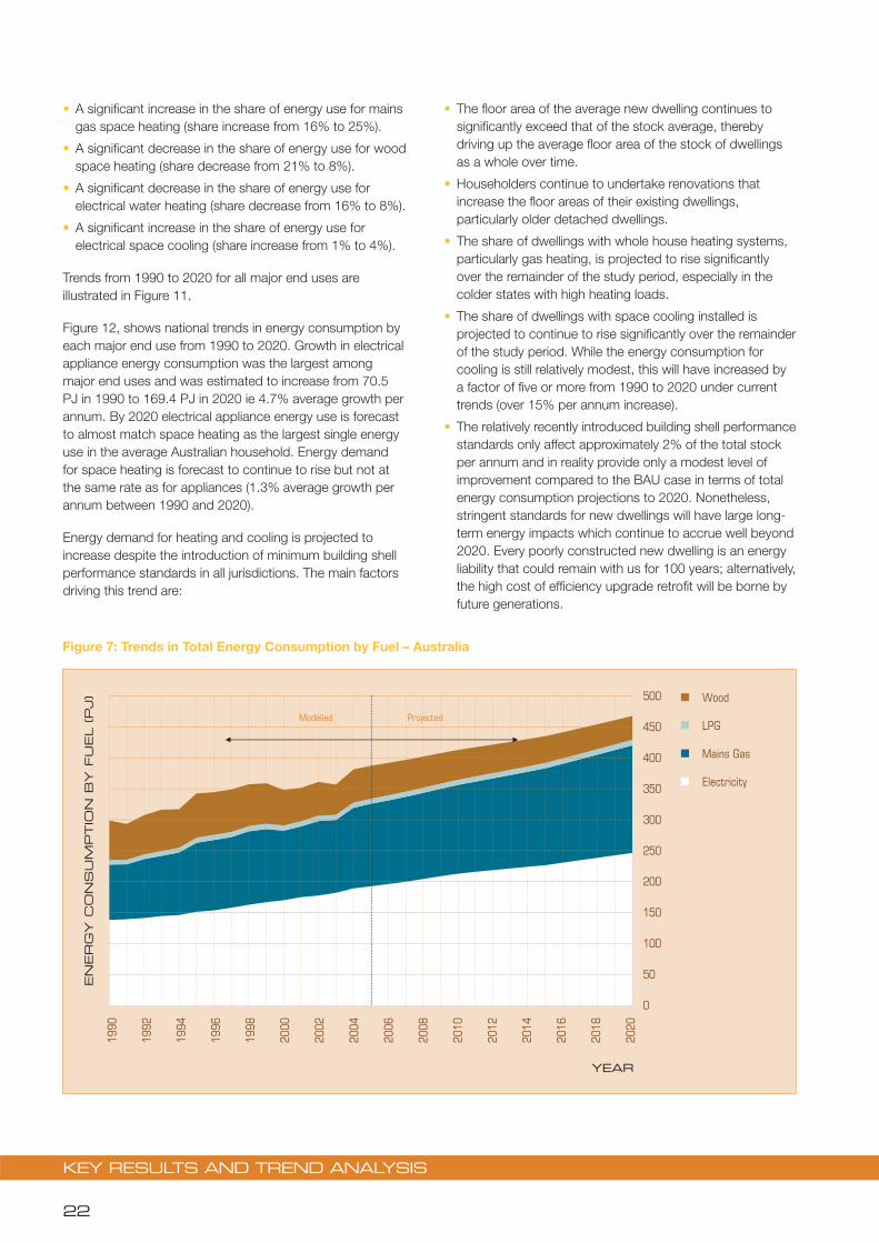
KEY RESULTS AND TREND ANALYSIS
22
A significant increase in the share of energy use for mains gas space heating (share increase from 16% to 25%).
A significant decrease in the share of energy use for wood space heating (share decrease from 21% to 8%).
A significant decrease in the share of energy use for electrical water heating (share decrease from 16% to 8%).
A significant increase in the share of energy use for electrical space cooling (share increase from 1% to 4%).
Trends from 1990 to 2020 for all major end uses are illustrated in Figure 11.
Figure 12, shows national trends in energy consumption by each major end use from 1990 to 2020. Growth in electrical appliance energy consumption was the largest among major end uses and was estimated to increase from 70.5 PJ in 1990 to 169.4 PJ in 2020 ie 4.7% average growth per annum. By 2020 electrical appliance energy use is forecast to almost match space heating as the largest single energy use in the average Australian household. Energy demand for space heating is forecast to continue to rise but not at the same rate as for appliances (1.3% average growth per annum between 1990 and 2020).
Energy demand for heating and cooling is projected to increase despite the introduction of minimum building shell performance standards in all jurisdictions. The main factors driving this trend are:
The floor area of the average new dwelling continues to significantly exceed that of the stock average, thereby driving up the average floor area of the stock of dwellings as a whole over time.
Householders continue to undertake renovations that increase the floor areas of their existing dwellings, particularly older detached dwellings.
The share of dwellings with whole house heating systems, particularly gas heating, is projected to rise significantly over the remainder of the study period, especially in the colder states with high heating loads.
The share of dwellings with space cooling installed is projected to continue to rise significantly over the remainder of the study period. While the energy consumption for cooling is still relatively modest, this will have increased by a factor of five or more from 1990 to 2020 under current trends (over 15% per annum increase).
The relatively recently introduced building shell performance standards only affect approximately 2% of the total stock per annum and in reality provide only a modest level of improvement compared to the BAU case in terms of total energy consumption projections to 2020. Nonetheless, stringent standards for new dwellings will have large long-term energy impacts which continue to accrue well beyond 2020. Every poorly constructed new dwelling is an energy liability that could remain with us for 100 years; alternatively, the high cost of efficiency upgrade retrofit will be borne by future generations.
0
50
100
150
200
250
300
350
400
450
500
1990
1992
1994
1996
1998
2000
2002
2004
2006
2008
2010
2012
2014
2016
2018
2020
YEAR
EN
ER
GY C
ON
SU
MPTIO
N B
Y F
UEL (PJ) Wood
LPG
Mains Gas
Electricity
Modelled Projected
Figure 7: Trends in Total Energy Consumption by Fuel – Australia

SECTION 3
23
Table 2: Total Energy Consumption in petajoules by Fuel by Year – Australia (EES)
Year Electricity Mains Gas LPG Wood Total
1990 138.3 89.2 7.5 63.8 298.8
1991 139.5 88.7 7.3 57.7 293.2
1992 141.5 95.0 7.6 63.3 307.3
1993 144.6 97.1 7.7 66.7 316.2
1994 146.1 101.0 7.6 62.2 316.9
1995 151.4 111.3 8.2 71.4 342.3
1996 153.7 113.6 8.2 68.9 344.5
1997 158.1 113.9 8.4 68.6 348.9
1998 162.9 118.4 8.5 67.4 357.2
1999 166.9 118.0 8.6 65.4 358.9
2000 170.1 112.2 8.4 57.3 348.1
2001 175.1 114.2 8.4 53.7 351.4
2002 177.8 120.0 8.7 54.5 361.0
2003 182.1 117.6 8.2 48.8 356.7
2004 189.2 130.0 8.4 53.6 381.2
2005 192.6 133.1 8.2 53.2 387.1
2006 196.3 134.9 8.3 52.3 391.7
2007 200.1 137.0 8.3 51.3 396.6
2008 204.3 139.0 8.3 50.2 401.9
2009 208.8 141.0 8.4 49.1 407.3
2010 213.1 143.1 8.4 48.1 412.7
2011 216.1 145.4 8.4 47.1 417.0
2012 218.8 147.9 8.5 46.1 421.2
2013 221.4 150.6 8.5 45.1 425.6
2014 224.1 153.4 8.6 44.1 430.2
2015 226.6 156.4 8.7 43.1 434.8
2016 230.6 159.6 8.8 42.1 441.1
2017 234.7 162.9 8.9 41.2 447.6
2018 238.6 166.3 9.0 40.2 454.1
2019 242.6 169.9 9.0 39.2 460.7
2020 246.4 173.6 9.1 38.2 467.4
Source: EES model outputs

KEY RESULTS AND TREND ANALYSIS
24
AppliancesElectricity, 69.0, 24%
Water heatingElectricity, 47.4, 16%
Water heatingMains Gas, 33.8, 11%
CookingMains Gas, 5.9, 2%
Space HeatingMains Gas, 48.0, 16%
AppliancesMains Gas, 1.5, 0%
Space CoolingElectricity, 3.0, 1%
Water heatingLPG, 2.9, 1%
CookingLPG, 1.1, 0%
Space HeatingWood, 63.8, 21%
CookingElectricity, 7.9, 3%
Space HeatingLPG, 3.5, 1%
Space HeatingElectricity, 10.9, 4%
AppliancesElectricity, 122.5, 31%
AppliancesMains Gas, 2.4, 1%
Water heatingMains Gas, 44.7, 11%
CookingMains Gas, 8.5, 2%
Space HeatingMains Gas, 81.3, 21%
Water heatingElectricity, 43.1, 11%
Space CoolingElectricity, 11.9, 3%
Space HeatingElectricity, 13.4, 3%
CookingElectricity, 9.3, 2%
Water heatingLPG, 2.9, 1%
CookingLPG, 1.8, 0%
Space HeatingWood, 51.3, 13%
Space HeatingLPG, 3.6, 1%
Figure 8: Breakdown of Energy for Major End Uses – 1990 Australia
Figure 9: Breakdown of Energy for Major End Uses – 2007 Australia
Note: Energy consumption shown in PJ followed by % share of total
Note: Energy consumption shown in PJ followed by % share of total

SECTION 3
25
Modelled ProjectedM e P t
0
50
100
150
200
250
300
350
400
450
500
1990
1992
1994
1996
1998
2000
2002
2004
2006
2008
2010
2012
2014
2016
2018
2020
YEAR
EN
ER
GY C
ON
SU
MPTIO
N (PJ) Wood Space Heating
LPG Space Heating
LPG Cooking
LPG Water heating
Mains Gas Space Heating
Mains Gas Cooking
Mains Gas Water heating
Mains Gas Appliances
Electricity Space Cooling
Electricity Space Heating
Electricity Cooking
Electricity Water heating
Electricity Appliances
AppliancesElectricity, 166.1, 36%
Water heatingMains Gas, 43.0, 9%
CookingMains Gas, 11.3, 2%
Space CoolingElectricity, 17.7, 4%
AppliancesMains Gas, 3.2, 1%
Space HeatingElectricity, 15.6, 3%
Water heatingElectricity, 37.6, 8%
Space HeatingMains Gas, 116.0, 25%
CookingElectricity, 9.4, 2%
Water heatingLPG, 2.8, 1%
Space HeatingWood, 38.2, 8%Cooking
LPG, 2.2, 0%
Space HeatingLPG, 4.1, 1%
Figure 10: Breakdown of Energy for Major End Uses – 2020 Australia
Figure 11: Trends in Total Energy Consumption by End Use – Australia
Note: Energy consumption shown in PJ followed by % share of total

KEY RESULTS AND TREND ANALYSIS
26
Figure 13: Trends in National Residential Floor Area and Number of Occupied Residential Households
Figure 12: Trends in Total Energy Consumption by Major End Use – Australia
Floor Area
OccupiedResidentialHouseholds
0
200
400
600
800
1000
1200
1400
1600
1800
1986
1988
1990
1992
1994
1996
1998
2000
2002
2004
2006
2008
2010
2012
2014
2016
2018
2020
YEAR
FLO
OR
AR
EA
(M
ILLIO
NS
OF M
2)
0.0
1.5
3.0
4.5
6.0
7.5
9.0
10.5
12.0
13.5
NU
MB
ER
HO
US
EH
OLD
S (M
ILLIO
N)
1990
1992
1994
1996
1998
2000
2002
2004
2006
2008
2010
2012
2014
2016
2018
2020
EN
ER
GY C
ON
SU
MPTIO
N (PJ) Appliances
Water Heating
Cooking
Space Heating
Space Cooling
Modelled Projected
YEAR
0
20
40
60
80
100
120
140
160
180
200

SECTION 3
27
The other major energy use, water heating, plateaued in 2004 and is expected to decline slowly to 2020. Notably this is the only major energy use predicted to decline over the study period, principally as a result of various energy programs undertaken by State and Federal governments. The key drivers for water heating are an increase in gas and solar technologies and declining demand for hot water from water-efficient appliances (front-loading washing machines and low-flow shower heads) as well as a decline in the number of people per household.
Cooking energy is forecast to undergo slow but steady growth of approximately 1.8% per annum over the study period, roughly in line with the growth in the number of households. There is a trend towards gas cook-tops and electric ovens which is driven by consumer preference and overall performance. Cooking energy consumption remains a modest share of total energy consumption.
Of all the major end uses, space cooling is forecast to show the most rapid growth over the study period with an average growth of about 16% per annum. This growth comes off a very low energy base of 3 PJ (1990), so even with this high rate of growth in total energy terms by 2020 energy consumption for space cooling is only 17.7 PJ or 4% of total residential energy consumption in that year.
However, despite its low contribution to total energy consumption, it is an end use that attracts considerable political and policy attention due to its very poor load factor and potential to create major problems for the electricity generation, transmission and distribution system on peak summer days. On summer days of maximum demand the space cooling loads typically account for one-third of total electrical system demand and in some states, such as SA, can account for as much as half the total system demand. Meet the cooling demand in the summer places a significant impost on governments in terms of infrastructure requirements. During extremely hot weather the electricity transmission and distribution system is at its lowest capacity. Various programs are examining options for “demand response” capability for air conditioners and other discretionary loads in order to redress some of these issues.
However, these are all peak load related issues and have negligible impact on overall energy consumption for these products. Building shell performance is the single most important driver for future air conditioning energy consumption, so performance requirements for new homes (or lack thereof) will ultimately drive future air conditioning demand. The rapid increase in air conditioner ownership over the past eight years was not foreshadowed and would appear to be driven by increasing wealth and lower costs for air conditioners. Perversely, perceptions of “climate change” making weather hotter together with an increase in the prevalence of extreme weather days may also be having some influence on the market.
Household projections and floor area3.2.4
As part of this study, estimates of household numbers and floor area were made from 1986 to 2020. Estimates for occupied residential households are presented in Table 10 (Section 5). Estimates for total floor area by state by year are presented in Table 3.
Figure 13 plots a time series from 1986 to 2020 of trends in national residential floor area (primary “y” axis, left) and national number of occupied residential households (secondary “y” axis, right). Growth in number of occupied households over the study period averages 1.7% per annum whereas over the same period, growth in total floor area averages 3.1% per annum (which equates to an effective increase in average per house floor area of 1.4% per annum).
Between 1990 and 2020 the number of occupied residential households is forecast to increase from six million to almost 10 million, an increase of 61%. Over the same period, total residential floor area is set to rise from 685 millions square metres to almost 1682 million square metres, an increase of 145%. Based on current trends, the average floor area of a dwelling in 2020 is estimated to be 50% higher than a dwelling in 1990, which has occurred despite declining household sizes (in terms of the number of occupants). This significant increase in floor area will impact significantly on some household energy end uses, in particular space conditioning and to a lesser extent lighting. Embodied energy per household would also undergo a significant increase over the study period, although this study makes no estimates of these impacts.
Energy trends per household and 3.2.5 per capital
By dividing the total residential energy consumption by the estimated number of households in the corresponding year, a trend in per household energy consumption can be derived.
Figure 14 shows that since 1990 energy consumption per household have remained fairly constant apart from the influence of year-to-year climatic variations that impact significantly on space conditioning energy demand. Projecting forward to 2020 there is expected to be a modest decline in energy consumption per household of approximately 6% compared to 1990 levels. This decline is achieved despite expected increases in service deliveries to households, particularly in space conditioning and in certain appliance types (eg larger more power intensive televisions, increased standby energy consumption, more lighting, more computers and other home entertainment). This decline is being driven mainly by existing and planned energy programs designed to improve appliance and building shell energy efficiency.
By comparison, if the total residential energy consumption in each year of the study period is divided by the population in the corresponding year, the trend in per person residential energy consumption shows a steady but modest increase from 17GJ/person in 1990 to 20GJ/person in 2020 or a 20% increase over the study period (Figure 15).

KEY RESULTS AND TREND ANALYSIS
28
Year NSW VIC QLD SA WA TAS NT ACT AUS
1986 202 155 98 54 54 18 4 9 594
1987 208 160 103 56 57 18 4 9 615
1988 214 164 109 57 60 19 5 10 637
1989 221 170 115 59 64 19 5 10 663
1990 227 174 121 61 66 20 5 10 685
1991 233 178 126 63 69 21 5 11 705
1992 240 182 133 64 72 21 5 11 729
1993 247 187 141 66 75 22 6 12 755
1994 255 193 150 68 79 22 6 12 785
1995 263 198 157 70 83 23 6 13 812
1996 270 202 163 71 86 23 6 13 834
1997 278 208 170 72 89 24 7 13 859
1998 287 214 177 74 92 24 7 14 888
1999 296 222 183 76 96 24 7 14 918
2000 305 231 191 78 100 25 7 15 952
2001 312 238 197 79 103 25 8 15 977
2002 322 247 205 81 107 26 8 15 1010
2003 331 255 214 83 111 26 8 16 1045
2004 341 264 223 86 116 27 8 17 1082
2005 349 273 232 88 121 27 9 17 1115
2006 359 281 242 90 126 28 9 18 1152
2007 369 290 252 91 130 29 9 18 1188
2008 380 298 262 93 135 29 10 18 1224
2009 390 306 271 95 139 30 10 19 1261
2010 400 315 282 97 144 30 10 19 1298
2011 411 323 292 99 149 31 11 20 1335
2012 421 332 302 101 154 31 11 20 1372
2013 432 340 313 103 158 32 11 21 1410
2014 443 349 323 105 163 33 12 21 1448
2015 453 357 334 107 168 33 12 22 1487
2016 464 366 345 109 173 34 12 22 1526
2017 475 375 356 111 178 34 13 23 1564
2018 486 384 367 112 183 35 13 23 1603
2019 497 393 378 114 188 35 13 24 1642
2020 507 401 390 116 193 36 14 24 1681
Table 3: Estimated Total Occupied Residential Floor Areas (million m2)

SECTION 3
29
Figure 14: Trends in Residential Energy Use per Household in Australia from 1990 to 2020
Figure 15: Trends in Residential Energy Use per Person in Australia from 1990 to 2020
30
35
40
45
50
55
1990
1991
1992
1993
1994
1995
1996
1997
1998
1999
2000
2001
2002
2003
2004
2005
2006
2007
2008
2009
2010
2011
2012
2013
2014
2015
2016
2017
2018
2019
2020
GJ / P
ER
HO
US
EH
OLD
Modelled Projected
YEAR
0
5
10
15
20
25
1990
1992
1994
1996
1998
2000
2002
2004
2006
2008
2010
2012
2014
2016
2018
2020
GJ / P
ER
PER
SO
N
Modelled Projected
YEAR

KEY RESULTS AND TREND ANALYSIS
30
Figure 16: Trends in Fuel Energy Consumption per Household
0
5
10
15
20
25
30
1990
1992
1994
1996
1998
2000
2002
2004
2006
2008
2010
2012
2014
2016
2018
2020
YEAREN
ER
GY C
ON
SU
MPTIO
N B
Y F
UEL (G
J/H
OU
SEH
OLD
) Electricity
Mains Gas
Wood
LPG
Modelled Projected
The trends in energy consumption per household by fuel show some interesting trends (Figure 16). At a national level, electricity, mains gas and LPG per household remain fairly steady from 1990 to 2020, while wood is projected to decrease significantly, mainly due to fuel switching away from this fuel for space heating. These trends are much more complex when examined at the state level.
The trend by major end use is more complex as shown in Figure 17. Electrical appliances are the only major end use that is showing strong growth at a household level. Mains gas space heating is fairly steady per household but is projected to show some growth particularly from 2010 onwards. Electric water heating, wood space heating and gas water heating are all showing strong decreases in energy per household, the first two due to fuel switching away to other fuel types and the latter due to the impact of new MEPS levels on energy consumption per appliance. Space cooling is also showing some growth, but from a low base. Other major end uses make fairly modest contributions to household energy consumption. Again, these trends at a state level are much more complex.
It could be observed that while existing and proposed energy programs are holding the line in terms of energy use at a household level, it is the significant increase in household numbers (61% increase from 1990 to 2020) that is driving the rapid growth of energy consumption of this sector as a whole (62% increase from 1990 to 2020). If population growth continues at present levels into the future (together
with an ongoing decline in household size), the inescapable conclusion is that, in the absence of substantial new policy measures, energy consumption from the residential sector will continue to rise at a significant rate.
Breakdown by state3.3 Table 4 and Figure 18 provide an overview of total energy consumption by state by year. Victoria, NSW and Queensland show steady growth over the study period. Despite having a lower population than NSW, Victoria has the highest energy consumption of any state. This higher than average per household energy consumption is primarily due to the extensive use of gas for space heating and the higher heating load from the cooler climate. In Victoria, winters are more severe than in NSW (or Queensland) and householders typically space heat their entire dwelling using ducted gas heating.
The following five tables with associated figures detail the energy consumption by major end use by state or territory. The major end uses detailed are:
Electrical Appliances (Table 5 and Figure 19)
Water Heating (Table 6 and Figure 20)
Cooking (Table 7 and Figure 21)
Space Heating (Table 8 and Figure 22)
Space Cooling (Table 9 and Figure 23).

SECTION 3
31
Table 4: Total Residential Energy Consumption in petajoules by State from 1990 to 2020
Year NSW VIC QLD SA WA TAS NT ACT AUS
1990 83.6 113.0 28.8 25.4 22.6 18.7 1.4 5.3 298.8
1991 82.4 110.4 29.1 24.4 22.5 17.7 1.4 5.2 293.2
1992 85.3 116.4 30.4 25.2 23.2 19.5 1.4 5.8 307.3
1993 89.4 115.9 31.3 26.3 24.9 20.6 1.4 6.5 316.2
1994 87.3 120.3 32.4 25.2 24.3 19.6 1.4 6.3 316.9
1995 92.9 132.5 34.5 26.6 26.8 20.8 1.5 6.7 342.3
1996 92.8 134.5 35.1 26.2 26.8 20.6 1.6 7.0 344.5
1997 95.0 133.4 36.8 26.8 27.4 20.5 1.7 7.2 348.9
1998 96.5 139.2 37.8 26.8 28.1 19.8 1.8 7.2 357.2
1999 97.8 137.6 38.3 27.3 28.4 20.1 1.9 7.6 358.9
2000 96.3 129.0 39.6 26.4 28.2 19.0 1.9 7.7 348.1
2001 96.4 131.1 41.1 26.8 28.4 17.8 1.9 7.8 351.4
2002 98.4 136.7 42.2 27.3 29.0 17.4 2.0 7.9 361.0
2003 97.7 133.3 43.4 27.0 28.9 16.2 2.1 8.1 356.7
2004 102.3 146.9 45.7 28.5 30.2 16.7 2.2 8.7 381.2
2005 103.7 149.0 46.6 28.4 31.5 16.6 2.2 9.1 387.1
2006 104.7 150.8 47.8 28.4 31.8 16.5 2.3 9.3 391.7
2007 105.9 152.7 49.0 28.5 32.2 16.5 2.3 9.6 396.6
2008 107.1 154.7 50.2 28.6 32.6 16.4 2.4 9.8 401.9
2009 108.5 156.7 51.5 28.8 33.0 16.4 2.4 10.0 407.3
2010 109.8 158.8 52.7 28.9 33.4 16.3 2.5 10.3 412.7
2011 110.7 160.7 53.6 29.0 33.7 16.2 2.5 10.5 417.0
2012 111.6 162.7 54.5 29.0 34.0 16.2 2.5 10.7 421.2
2013 112.5 164.8 55.4 29.1 34.2 16.1 2.6 10.9 425.6
2014 113.4 167.0 56.3 29.1 34.5 16.0 2.6 11.1 430.2
2015 114.3 169.3 57.2 29.2 34.8 16.0 2.7 11.4 434.8
2016 115.6 172.0 58.4 29.4 35.3 16.0 2.7 11.6 441.1
2017 117.0 174.8 59.7 29.5 35.8 15.9 2.8 11.9 447.6
2018 118.4 177.6 61.0 29.7 36.3 15.9 2.9 12.2 454.1
2019 119.8 180.6 62.3 29.9 36.8 15.9 2.9 12.5 460.7
2020 121.2 183.5 63.5 30.1 37.4 15.9 3.0 12.8 467.4

KEY RESULTS AND TREND ANALYSIS
32
Figure 18: Trends in Total Residential Energy Consumption by State from 1990 to 2020
Modelled ProjectedM e o e
0
20
40
60
80
100
120
140
160
180
200
1990
1992
1994
1996
1998
2000
2002
2004
2006
2008
2010
2012
2014
2016
2018
2020
YEAR
EN
ER
GY C
ON
SU
MPTIO
N (PJ) NSW
VIC
QLD
SA
WA
TAS
NT
ACT
Figure 17: Trends in Major End-Use Energy per Household – Australia
Modelled Projectedo l o e
0
2
4
6
8
10
12
14
16
18
1990
1992
1994
1996
1998
2000
2002
2004
2006
2008
2010
2012
2014
2016
2018
2020
YEAR
EN
ER
GY C
ON
SU
MPTIO
N (G
J/H
OU
SEH
OLD
) Electrical Appliances
Mains Gas Space Heating
Wood Space Heating
Electrical Water heating
Mains Gas Water heating
Electricity Space Cooling
Electricity Space Heating
Mains Gas Cooking
Electricity Cooking
LPG Space Heating
Mains Gas Appliances
LPG Water heating
LPG Cooking

SECTION 3
33
Table 5: Electrical Appliance Energy Consumption in petajoules by State from 1990 to 2020
Year NSW VIC QLD SA WA TAS NT ACT AUS
1990 24.4 18.0 11.9 6.1 6.4 1.9 0.6 1.1 70.5
1991 25.1 18.4 12.4 6.3 6.6 2.0 0.6 1.1 72.5
1992 25.8 18.8 13.1 6.4 6.8 2.1 0.6 1.2 74.8
1993 26.5 19.3 13.8 6.6 7.1 2.1 0.7 1.3 77.4
1994 27.3 19.9 14.6 6.8 7.5 2.2 0.7 1.3 80.2
1995 28.3 20.4 15.4 6.9 7.8 2.2 0.7 1.3 83.1
1996 29.2 20.9 16.1 7.1 8.1 2.3 0.7 1.4 85.9
1997 30.4 21.7 17.0 7.3 8.5 2.3 0.8 1.4 89.4
1998 31.7 22.6 17.9 7.5 8.9 2.4 0.8 1.5 93.3
1999 32.9 23.4 18.7 7.7 9.3 2.5 0.9 1.6 96.9
2000 34.1 24.3 19.4 8.0 9.8 2.5 0.9 1.6 100.5
2001 34.9 25.0 20.0 8.2 10.2 2.6 0.9 1.7 103.4
2002 36.2 25.9 20.7 8.5 10.6 2.6 0.9 1.7 107.1
2003 37.4 26.7 21.6 8.7 11.0 2.7 1.0 1.8 110.8
2004 38.6 27.5 22.6 9.0 11.4 2.8 1.0 1.8 114.7
2005 39.5 28.3 23.4 9.2 11.9 2.9 1.0 1.9 118.0
2006 40.4 29.0 24.3 9.3 12.3 2.9 1.1 1.9 121.2
2007 41.5 29.8 25.2 9.5 12.7 3.0 1.1 2.0 124.8
2008 42.7 30.7 26.2 9.8 13.2 3.1 1.1 2.0 128.8
2009 44.0 31.8 27.2 10.1 13.7 3.2 1.2 2.1 133.1
2010 45.3 32.8 28.3 10.3 14.2 3.2 1.2 2.1 137.5
2011 46.2 33.5 29.1 10.5 14.5 3.3 1.2 2.2 140.5
2012 47.0 34.1 29.8 10.6 14.8 3.3 1.2 2.2 143.2
2013 47.8 34.7 30.5 10.8 15.1 3.4 1.3 2.3 145.8
2014 48.6 35.2 31.2 10.9 15.4 3.4 1.3 2.3 148.3
2015 49.3 35.7 31.9 11.0 15.7 3.4 1.3 2.3 150.8
2016 50.5 36.6 32.9 11.2 16.1 3.5 1.3 2.4 154.6
2017 51.7 37.4 34.0 11.4 16.6 3.6 1.4 2.4 158.5
2018 52.8 38.3 35.0 11.6 17.0 3.6 1.4 2.5 162.2
2019 53.9 39.1 36.0 11.8 17.5 3.7 1.4 2.5 165.9
2020 55.0 39.8 37.0 12.0 17.9 3.7 1.5 2.6 169.4

KEY RESULTS AND TREND ANALYSIS
34
Figure 19: Electrical Appliance Energy Consumption Trends by State from 1990 to 2020
Figure 20: Water Heating Energy Consumption Trends by State from 1990 to 2020
0
10
20
30
40
50
60
1990
1992
1994
1996
1998
2000
2002
2004
2006
2008
2010
2012
2014
2016
2018
2020
YEAR
EN
ER
GY C
ON
SU
MPTIO
N (PJ) NSW
VIC
QLD
SA
WA
TAS
NT
ACT
0
5
10
15
20
25
30
35
1990
1992
1994
1996
1998
2000
2002
2004
2006
2008
2010
2012
2014
2016
2018
2020
YEAR
EN
ER
GY C
ON
SU
MPTIO
N (PJ) NSW
VIC
QLD
SA
WA
TAS
NT
ACT
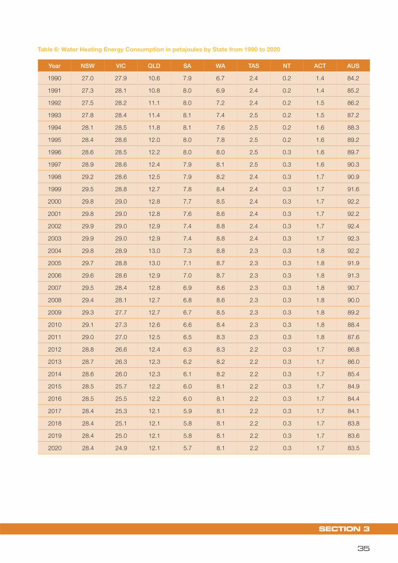
SECTION 3
35
Table 6: Water Heating Energy Consumption in petajoules by State from 1990 to 2020
Year NSW VIC QLD SA WA TAS NT ACT AUS
1990 27.0 27.9 10.6 7.9 6.7 2.4 0.2 1.4 84.2
1991 27.3 28.1 10.8 8.0 6.9 2.4 0.2 1.4 85.2
1992 27.5 28.2 11.1 8.0 7.2 2.4 0.2 1.5 86.2
1993 27.8 28.4 11.4 8.1 7.4 2.5 0.2 1.5 87.2
1994 28.1 28.5 11.8 8.1 7.6 2.5 0.2 1.6 88.3
1995 28.4 28.6 12.0 8.0 7.8 2.5 0.2 1.6 89.2
1996 28.6 28.5 12.2 8.0 8.0 2.5 0.3 1.6 89.7
1997 28.9 28.6 12.4 7.9 8.1 2.5 0.3 1.6 90.3
1998 29.2 28.6 12.5 7.9 8.2 2.4 0.3 1.7 90.9
1999 29.5 28.8 12.7 7.8 8.4 2.4 0.3 1.7 91.6
2000 29.8 29.0 12.8 7.7 8.5 2.4 0.3 1.7 92.2
2001 29.8 29.0 12.8 7.6 8.6 2.4 0.3 1.7 92.2
2002 29.9 29.0 12.9 7.4 8.8 2.4 0.3 1.7 92.4
2003 29.9 29.0 12.9 7.4 8.8 2.4 0.3 1.7 92.3
2004 29.8 28.9 13.0 7.3 8.8 2.3 0.3 1.8 92.2
2005 29.7 28.8 13.0 7.1 8.7 2.3 0.3 1.8 91.9
2006 29.6 28.6 12.9 7.0 8.7 2.3 0.3 1.8 91.3
2007 29.5 28.4 12.8 6.9 8.6 2.3 0.3 1.8 90.7
2008 29.4 28.1 12.7 6.8 8.6 2.3 0.3 1.8 90.0
2009 29.3 27.7 12.7 6.7 8.5 2.3 0.3 1.8 89.2
2010 29.1 27.3 12.6 6.6 8.4 2.3 0.3 1.8 88.4
2011 29.0 27.0 12.5 6.5 8.3 2.3 0.3 1.8 87.6
2012 28.8 26.6 12.4 6.3 8.3 2.2 0.3 1.7 86.8
2013 28.7 26.3 12.3 6.2 8.2 2.2 0.3 1.7 86.0
2014 28.6 26.0 12.3 6.1 8.2 2.2 0.3 1.7 85.4
2015 28.5 25.7 12.2 6.0 8.1 2.2 0.3 1.7 84.9
2016 28.5 25.5 12.2 6.0 8.1 2.2 0.3 1.7 84.4
2017 28.4 25.3 12.1 5.9 8.1 2.2 0.3 1.7 84.1
2018 28.4 25.1 12.1 5.8 8.1 2.2 0.3 1.7 83.8
2019 28.4 25.0 12.1 5.8 8.1 2.2 0.3 1.7 83.6
2020 28.4 24.9 12.1 5.7 8.1 2.2 0.3 1.7 83.5

KEY RESULTS AND TREND ANALYSIS
36
Year NSW VIC QLD SA WA TAS NT ACT AUS
1990 4.8 4.2 2.3 1.4 1.5 0.3 0.1 0.2 14.8
1991 4.9 4.3 2.4 1.4 1.5 0.4 0.1 0.2 15.1
1992 5.0 4.4 2.4 1.4 1.6 0.4 0.1 0.2 15.5
1993 5.1 4.5 2.5 1.4 1.6 0.4 0.1 0.2 15.9
1994 5.2 4.5 2.6 1.5 1.7 0.4 0.1 0.2 16.2
1995 5.3 4.6 2.7 1.5 1.7 0.4 0.1 0.3 16.6
1996 5.4 4.6 2.8 1.5 1.8 0.4 0.1 0.3 16.8
1997 5.4 4.7 2.8 1.5 1.8 0.4 0.1 0.3 17.0
1998 5.5 4.8 2.9 1.5 1.8 0.4 0.1 0.3 17.3
1999 5.6 4.8 3.0 1.5 1.9 0.4 0.1 0.3 17.6
2000 5.7 4.9 3.0 1.6 1.9 0.4 0.1 0.3 17.9
2001 5.8 5.0 3.1 1.6 1.9 0.4 0.1 0.3 18.1
2002 5.8 5.0 3.1 1.6 1.9 0.4 0.1 0.3 18.4
2003 5.9 5.1 3.2 1.6 2.0 0.4 0.2 0.3 18.6
2004 6.0 5.2 3.2 1.6 2.0 0.4 0.2 0.3 18.9
2005 6.0 5.2 3.3 1.7 2.1 0.4 0.2 0.3 19.1
2006 6.1 5.3 3.4 1.7 2.1 0.4 0.2 0.3 19.4
2007 6.2 5.3 3.4 1.7 2.1 0.4 0.2 0.3 19.7
2008 6.3 5.4 3.5 1.7 2.2 0.4 0.2 0.3 19.9
2009 6.3 5.5 3.6 1.7 2.2 0.4 0.2 0.3 20.2
2010 6.4 5.5 3.6 1.7 2.2 0.4 0.2 0.3 20.4
2011 6.5 5.6 3.7 1.7 2.3 0.4 0.2 0.3 20.7
2012 6.6 5.6 3.8 1.7 2.3 0.4 0.2 0.3 20.9
2013 6.7 5.7 3.8 1.7 2.3 0.4 0.2 0.3 21.2
2014 6.7 5.7 3.9 1.8 2.4 0.4 0.2 0.4 21.4
2015 6.8 5.8 4.0 1.8 2.4 0.4 0.2 0.4 21.7
2016 6.9 5.8 4.0 1.8 2.4 0.4 0.2 0.4 21.9
2017 7.0 5.9 4.1 1.8 2.5 0.4 0.2 0.4 22.2
2018 7.1 5.9 4.2 1.8 2.5 0.4 0.2 0.4 22.4
2019 7.1 6.0 4.3 1.8 2.5 0.4 0.2 0.4 22.7
2020 7.2 6.0 4.3 1.8 2.6 0.4 0.2 0.4 22.9
Table 7: Cooking Energy Consumption in petajoules by State from 1990 to 2020

SECTION 3
37
Figure 21: Cooking Energy Consumption Trends by State from 1990 to 2020
Figure 22: Space Heating Energy Consumption Trends by State from 1990 to 2020
0
1
2
3
4
5
6
7
8
1990
1992
1994
1996
1998
2000
2002
2004
2006
2008
2010
2012
2014
2016
2018
2020
YEAR
EN
ER
GY C
ON
SU
MPTIO
N (PJ) NSW
VIC
QLD
SA
WA
TAS
NT
ACT
0
20
40
60
80
100
120
1990
1992
1994
1996
1998
2000
2002
2004
2006
2008
2010
2012
2014
2016
2018
2020
YEAR
EN
ER
GY C
ON
SU
MPTIO
N (PJ) NSW
VIC
QLD
SA
WA
TAS
NT
ACT

KEY RESULTS AND TREND ANALYSIS
38
Table 8: Space Heating Energy Consumption in petajoules by State from 1990 to 2020
Year NSW VIC QLD SA WA TAS NT ACT AUS
1990 26.6 62.6 3.4 9.4 7.7 14.0 0.0 2.6 126.2
1991 24.0 59.3 2.8 8.2 7.1 13.0 0.0 2.4 116.7
1992 26.2 64.8 3.1 8.9 7.4 14.7 0.0 2.9 128.0
1993 29.1 63.3 2.9 9.8 8.4 15.7 0.0 3.5 132.7
1994 25.9 67.2 2.7 8.5 7.3 14.6 0.0 3.2 129.4
1995 30.1 78.5 3.5 9.6 9.1 15.7 0.0 3.5 150.1
1996 28.8 80.2 3.1 9.2 8.6 15.5 0.0 3.7 149.0
1997 29.3 78.0 3.7 9.6 8.7 15.4 0.0 3.8 148.5
1998 28.8 82.8 3.1 9.4 8.8 14.5 0.0 3.8 151.2
1999 28.6 80.1 2.6 9.6 8.3 14.8 0.0 4.0 148.0
2000 25.5 70.2 3.1 8.4 7.3 13.7 0.0 4.1 132.3
2001 23.8 71.4 3.2 8.3 6.7 12.5 0.0 4.1 130.0
2002 24.8 76.4 3.1 9.3 7.2 12.0 0.0 4.2 136.9
2003 22.3 71.9 3.2 8.3 6.3 10.7 0.0 4.2 126.9
2004 24.9 84.6 3.1 9.6 7.0 11.1 0.0 4.7 145.0
2005 25.4 85.9 3.3 9.2 7.7 11.0 0.0 5.0 147.6
2006 25.3 87.1 3.2 9.1 7.6 10.9 0.0 5.2 148.5
2007 25.2 88.4 3.2 9.1 7.5 10.8 0.0 5.4 149.5
2008 25.1 89.7 3.2 9.0 7.4 10.6 0.0 5.6 150.6
2009 25.0 90.9 3.2 9.0 7.3 10.5 0.0 5.8 151.7
2010 24.9 92.3 3.2 9.0 7.3 10.4 0.0 5.9 152.9
2011 24.9 93.8 3.2 9.0 7.2 10.2 0.0 6.1 154.4
2012 24.9 95.5 3.2 8.9 7.2 10.1 0.0 6.3 156.1
2013 24.9 97.3 3.2 8.9 7.1 10.0 0.0 6.5 157.9
2014 24.9 99.2 3.2 8.9 7.1 10.0 0.0 6.7 159.9
2015 25.0 101.1 3.2 8.9 7.1 9.9 0.0 6.9 162.0
2016 25.0 103.1 3.2 8.9 7.1 9.8 0.0 7.1 164.2
2017 25.1 105.2 3.2 9.0 7.1 9.7 0.0 7.3 166.6
2018 25.1 107.4 3.2 9.0 7.0 9.7 0.0 7.6 169.0
2019 25.2 109.5 3.2 9.0 7.0 9.6 0.0 7.8 171.4
2020 25.3 111.8 3.2 9.1 7.0 9.5 0.0 8.0 173.9
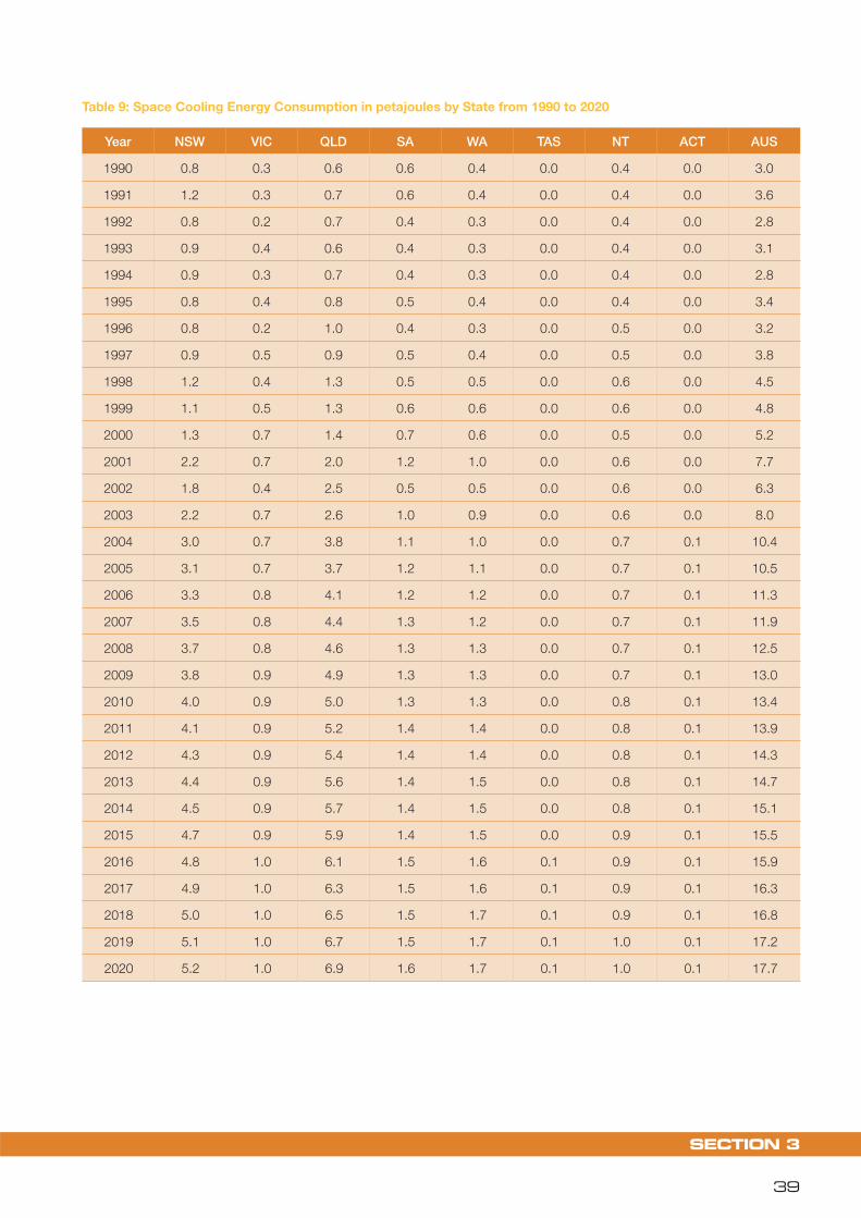
SECTION 3
39
Table 9: Space Cooling Energy Consumption in petajoules by State from 1990 to 2020
Year NSW VIC QLD SA WA TAS NT ACT AUS
1990 0.8 0.3 0.6 0.6 0.4 0.0 0.4 0.0 3.0
1991 1.2 0.3 0.7 0.6 0.4 0.0 0.4 0.0 3.6
1992 0.8 0.2 0.7 0.4 0.3 0.0 0.4 0.0 2.8
1993 0.9 0.4 0.6 0.4 0.3 0.0 0.4 0.0 3.1
1994 0.9 0.3 0.7 0.4 0.3 0.0 0.4 0.0 2.8
1995 0.8 0.4 0.8 0.5 0.4 0.0 0.4 0.0 3.4
1996 0.8 0.2 1.0 0.4 0.3 0.0 0.5 0.0 3.2
1997 0.9 0.5 0.9 0.5 0.4 0.0 0.5 0.0 3.8
1998 1.2 0.4 1.3 0.5 0.5 0.0 0.6 0.0 4.5
1999 1.1 0.5 1.3 0.6 0.6 0.0 0.6 0.0 4.8
2000 1.3 0.7 1.4 0.7 0.6 0.0 0.5 0.0 5.2
2001 2.2 0.7 2.0 1.2 1.0 0.0 0.6 0.0 7.7
2002 1.8 0.4 2.5 0.5 0.5 0.0 0.6 0.0 6.3
2003 2.2 0.7 2.6 1.0 0.9 0.0 0.6 0.0 8.0
2004 3.0 0.7 3.8 1.1 1.0 0.0 0.7 0.1 10.4
2005 3.1 0.7 3.7 1.2 1.1 0.0 0.7 0.1 10.5
2006 3.3 0.8 4.1 1.2 1.2 0.0 0.7 0.1 11.3
2007 3.5 0.8 4.4 1.3 1.2 0.0 0.7 0.1 11.9
2008 3.7 0.8 4.6 1.3 1.3 0.0 0.7 0.1 12.5
2009 3.8 0.9 4.9 1.3 1.3 0.0 0.7 0.1 13.0
2010 4.0 0.9 5.0 1.3 1.3 0.0 0.8 0.1 13.4
2011 4.1 0.9 5.2 1.4 1.4 0.0 0.8 0.1 13.9
2012 4.3 0.9 5.4 1.4 1.4 0.0 0.8 0.1 14.3
2013 4.4 0.9 5.6 1.4 1.5 0.0 0.8 0.1 14.7
2014 4.5 0.9 5.7 1.4 1.5 0.0 0.8 0.1 15.1
2015 4.7 0.9 5.9 1.4 1.5 0.0 0.9 0.1 15.5
2016 4.8 1.0 6.1 1.5 1.6 0.1 0.9 0.1 15.9
2017 4.9 1.0 6.3 1.5 1.6 0.1 0.9 0.1 16.3
2018 5.0 1.0 6.5 1.5 1.7 0.1 0.9 0.1 16.8
2019 5.1 1.0 6.7 1.5 1.7 0.1 1.0 0.1 17.2
2020 5.2 1.0 6.9 1.6 1.7 0.1 1.0 0.1 17.7

KEY RESULTS AND TREND ANALYSIS
40
Appliances3.4 Appliances and equipment represent a large range of diverse products in households. Many of these do not use substantial amounts of energy, but there are a few end uses that are of particular concern. Figure 24 provides details of trends in national electrical appliance energy usage by type of appliance.
The most important observations from Figure 24 are:
Television energy consumption is set to grow very rapidly (noting that this projection does not include MEPS levels or energy labelling proposed for 2010 as the levels are not yet finalised). This is being driven by the growth in LCD screen sales which will dominate the market within a few years and the average screen size is increasing rapidly.Refrigerator and freezer energy is declining due to the impact of 2005 MEPS and the ongoing pressure from energy labelling to reduce energy consumption.
Computers and related equipment will expand significantly (although most of the growth in ownership has already occurred, but there is potential through increased energy efficiency).
“Other standby” is likely to grow (noting that this does not include standby for individual products that are separately modelled). This is of significant concern as the mandatory one-watt target has already been modelled for most products.
Lighting is likely to grow significantly even with the incandescent lamp phase out which has been included in the projections.
Some of the underlying issues by end use are discussed in Section 4. More detail on modelling inputs is provided in Section 6.
Cooking3.5 Cooking energy contributed to only 5% of total energy consumption. The trend is for increasing gas cook-tops and increasing electric ovens, so energy is fairly evenly split between mains gas and electricity, with 10% LPG. However, the trends suggest that total electricity consumption will remain fairly steady (ovens increasing and cook-tops decreasing) while the gas consumption (natural gas and LPG) is forecast to grow slightly (Figure 25), mainly through increased use of gas cook-tops.
Water heating3.6 Water heating is a difficult end use to model as there are a wide range of possible water heater types. Solar systems are complex and have substantial energy interactions with both the user and the climate, which are difficult to model. There are a number of state-based programs that are likely to have a large impact on future ownership trends for the various water heater types. These issues are discussed in more detail in Section 6.
Figure 26 shows overall trends by water heater type. The analysis undertaken for this project is innovative in that the solar contribution for each solar water heater type is explicitly modelled and included in the total water heater energy (this is not included in the fuel consumption totals for Australia, shown as orange band at the top). By 2020 the solar contribution is projected to be nearly 8 PJ. This is despite the very modest increase in solar share forecast in the base case to 2020.
The projected hot water use per household is expected to decline gradually over time with declining household size and as improvements in water efficiency of clothes washers6 and shower heads take effect. Historically, electric water heaters have dominated the water heater market, but in recent years their share has declined and this trend is expected to continue. Energy consumption for electric storage water heaters is also continuing to decline slightly due to the impacts of both the 1999 and 2005 MEPS. Gas water heaters appear to have constant energy consumption over time, despite an increase in ownership. This is because efficiency improvements from MEPS (assumed to be introduced in 2008) more or less counteract growth in household numbers as well as fuel switching from electricity to gas. Solar water heaters are projected to grow and the solar contribution is substantially larger than the boost energy required to supplement these water heaters.
Space conditioning3.7
Space heating3.7.1
Space heating is one of the largest single end uses in the residential sector in Australia and currently accounts for 38% of total energy consumption (2007). The majority of the energy growth has been in mains gas. Victoria dominates national gas space heating energy consumption and there is a significant trend from room heating to central ducted space heating (mainly in Victoria) which has a higher zoning level and hence higher energy consumption per household. Wood as a heating fuel is declining slightly, although it is still significant. Electricity plays a small role in space heating (around 3.4% of total energy, 9% of space heating energy) although there is a shift from resistive heating to reverse-cycle air conditioning (heat pumps) within the electric fuel type, which suggests that the share of useful energy supplied by electricity for space heating is growing somewhat (the nominal efficiency of a heat pump is 2.5 to three times that of a resistive heater which is virtually 100%). However, electric heating is usually used in milder climates (apart from Tasmania) so the overall contribution to total energy is modest.
6 The share of front-loader (drum) clothes washer sales is approaching 50% in 2007. This will reduce the hot water used for warm washing as the total water consumption for this type is usually much lower than many top loaders, but also because in 2006 only 50% of front-loading models had the capability to be connected to hot and cold water supplies (meaning that any water heating is done using the electricity supply rather than the water heater). See Section 6 for more discussion.

SECTION 3
41
Figure 23: Space Cooling Energy Consumption Trends by State from 1990 to 2020
Figure 24: Trends in Electrical Appliance Energy by Type – Australia
0
1
2
3
4
5
6
7
8
1990
1992
1994
1996
1998
2000
2002
2004
2006
2008
2010
2012
2014
2016
2018
2020
YEAR
EN
ER
GY C
ON
SU
MPTIO
N (PJ) NSW
VIC
QLD
SA
WA
TAS
NT
ACT
0
20
40
60
80
100
120
140
160
180
1986
1988
1990
1992
1994
1996
1998
2000
2002
2004
2006
2008
2010
2012
2014
2016
2018
2020
YEAR
EN
ER
GY C
ON
SU
MPTIO
N (PJ) Miscell.
LightingOther SbyKettlesWaterbedSpasPoolsMisc. ITUMisc. ITSLaptopsMonitorsPCGamesHome entSTB PAYSTB FTADVDVCRTVMicrowaveDWCDCW frontCW topFZRF

KEY RESULTS AND TREND ANALYSIS
42
The impact of weather from year-to-year on energy consumption is quite marked for gas and wood, but less obvious for electric space heating and heat pumps, partly because these tend to be used more in milder climates with lower overall heating loads, but also because of the lower zoning levels for these types of heaters. Figure 27 depicts the trends in space heating energy. Note that after 2004 the default AccuRate weather input file has been used for every year from 2005 to 2020 (hence the smooth curve after this date).
Unlike other end uses examined in this study, space conditioning energy consumption is climate sensitive and as such varies significantly from state-to-state. For space heating, it is the cooler climates that generally dominate. Victoria, with a smaller population than NSW, accounts for a 59% share of national space heating energy consumption in 2007 compared with 17% for NSW (Figure 28). Tasmania with only 2.5 % of all households accounts for 7% of the space heating energy consumption. Victoria and Tasmania exhibit similar space heating energy consumption rates per household but Tasmania is a colder climate compared to Victoria.
This apparent anomaly is mainly a result of the fact that Victorian households generally demand higher standards of heating. Over 40% of Victorian households used central ducted gas heating in 2007 compared to virtually none in Tasmania. Tasmanian households do use a significant amount of wood heating (34.5% of homes in 2007 compared to 10% in Victoria) but taken together these two forms of whole house heating are significantly higher in Victoria (52%) compared to Tasmania (35%). The other heating types prevalent in Tasmania are not capable of whole house heating in most cases and so zoning factors reduce the estimated total energy.
Space cooling3.7.2
Space cooling is a product that attracts much attention from energy policy makers, but in fact is only responsible for a small share of total energy consumption (about 3% of total energy and 8.7% of electricity consumption in 2007). One of the issues that receive significant attention is their contribution to electricity supply system peak loads. However, this study does not examine that issue. Energy consumption for air conditioning is dominated by Queensland, with NSW also using significant energy. Most other states have relatively small total energy consumption for air conditioning over the projection period, despite large increases in penetration and ownership. This is due to the very modest cooling requirements in these other states.
Air conditioner ownership was almost flat through the 1990s, but from 1999 the ownership increased rapidly in most states. This rapid growth in ownership resulted in a commensurate growth in energy consumption, a trend expected to continue through to the end of the study period (Figure 29). The majority of units that make up the stock are split system (non-ducted) reverse cycle (the units make up the majority of the type RRCC). At present, total air conditioner sales are about one million units per year (noting that about one-third of these are commercial-sector sales).
As with space heating, space cooling energy consumption is climate sensitive and as such varies significantly from state-to-state. For space cooling, it is the warmer climates that generally dominate. In 2007, Queensland, with a smaller population than NSW, accounted for a 36% share of space cooling energy consumption compared to 29% for NSW (Figure 30).
Building shell efficiency3.7.3
The national trend for building shell efficiency (ie total potential space conditioning load per square metre of floor area), shows a modest but steady improvement over the study period, down from 280 MJ/m2 to approximately 200 MJ/m2 (Figure 31).
The national residential building shell efficiency improvement trend is being driven by policy initiatives that commenced in Victoria and ACT in 1990 and by 2005 had expanded to include all states through the BCA.
Unfortunately over the study period the rate of increase in average floor area has outpaced the rate of improvement in building shell efficiency to the extent that on a per household basis the potential space conditioning load (ie whole house heating and cooling in accordance with the default schedules of operation in the AccuRate software) is projected to increase from about 30 GJ to 35 GJ per household per annum (Figure 31) (secondary “y” axis, right, blue line).

SECTION 3
43
Figure 25: Trends in Cooking Energy by Type – Australia
Modelled Projectedo d r e
0
5
10
15
20
25
1986
1988
1990
1992
1994
1996
1998
2000
2002
2004
2006
2008
2010
2012
2014
2016
2018
2020
YEAR
CO
OK
ING
EN
ER
GY (PJ) Cook LPG
Oven LPG
Cook gas
Oven gas
Cook El
Oven El
0
10
20
30
40
50
60
70
80
90
100
1986
1988
1990
1992
1994
1996
1998
2000
2002
2004
2006
2008
2010
2012
2014
2016
2018
2020
YEAR
HO
T W
ATER
EN
ER
GY (PJ) Solar GI A
Solar GS A
Solar HP A
Solar El A
Solar GI B
Solar GS B
Solar HP B
Solar El B
LPG Inst
LPG Stor
Gas Inst
Gas Stor
Electric
Modelled Projectede r e
Figure 26: Trends in Water Heater Energy by Type – Australia

KEY RESULTS AND TREND ANALYSIS
44
Figure 28: Space Heating Share by State – 2007
Figure 27: Trends in Space Heating Energy by Fuel Type – Australia
NSW17%
VIC59%
QLD2%
SA6%
WA5%
TAS7%
NT
0%
ACT4%
Modelled Projected
0
20
40
60
80
100
120
140
160
180
200
1986
1988
1990
1992
1994
1996
1998
2000
2002
2004
2006
2008
2010
2012
2014
2016
2018
2020
YEAR
HEA
TIN
G E
NER
GY (PJ)
Wood O
Wood C
RoomLPG
Ductgas
Room Gas
DuctRCH
RRCH
El Resist
M e t

SECTION 3
45
Figure 30: Space Cooling Energy by Type State – 2008
Figure 29: Trends in Space Cooling Energy by Type – Australia
NSW29%
VIC7%
QLD36%
SA11%
WA10%
TAS0%
NT6%
ACT1%
Modelled Pr jected
0
2
4
6
8
10
12
14
16
18
20
1986
1988
1990
1992
1994
1996
1998
2000
2002
2004
2006
2008
2010
2012
2014
2016
2018
2020
YEAR
CO
OLIN
G E
NER
GY (PJ) Evap
DuctC
RCOC
RRCC
M e d

KEY RESULTS AND TREND ANALYSIS
46
Figure 31: Trends in Building Shell Efficiency in Australia from 1986 to 2020
Modelled ProjectedM d r d
0
50
100
150
200
250
300
350
400
1986
1988
1990
1992
1994
1996
1998
2000
2002
2004
2006
2008
2010
2012
2014
2016
2018
2020
YEAR
SH
ELL E
FFIC
IEN
CY (M
J/M
2)
0
5
10
15
20
25
30
35
40
SH
ELL E
FFIC
IEN
CY (G
J/H
HO
LD
) MJ/m2
GJ/H HoldTrend MJ/m2
Trend GJ/H Hold

RESULTS BY END USE
SECTION 4

RESULTS BY END USE
48
RESULTS BY END USE4
Overview4.1 This section provides selected details of energy demand by individual end use. Generally, end-use data in this section is presented at a national level, however, the data at a state level is presented in appendices of this report.
National trends in energy consumption by major end use (Figure 32) indicate that electrical appliances dominate total energy consumption throughout the study period. Electrical appliances not only represent the largest single end use in terms of energy consumption but have shown a strong growth trend in relative terms over the whole study period, rising from approximately one-quarter of all energy use in 1990 to one-third of all energy use projected for 2020. Given the high greenhouse gas coefficient for electricity production in most states, this means that electrical appliances dominate total greenhouse emissions from residential energy consumption.
Gas space heating is the next most significant end use, which has also shown significant growth over the study period. This growth is partly due to an expansion of the gas reticulation network and also the increase in the share of whole-house gas ducted heating (especially in Victoria). The increase in the use of gas for space heating also mirrors the decline in wood space heating energy over the same period.
Electric and gas water heating are the other two major end uses of energy. Energy consumption for both of these end
uses is projected to decline under the influence of various factors, including the impact of labelling and various MEPS programs, together with the expected increasing contribution of solar energy due to projected ownership increases in solar water heaters arising from recent changes in state policies for new homes.
Of the remaining end uses, space cooling is notable for its rapid growth over the study period, albeit from a modest base.
More details on the attributes and ownership by appliance type, together with other relevant data used for modelling inputs, are available in Section 6.
Space cooling equipment4.2 Since the late 1990s energy use by air conditioners has shown significant growth (Figure 33). This growth is being driven by substantial increases in ownership in all states, particularly of reverse-cycle room conditioners (primarily split-type systems).
In 1986 space cooling energy consumption accounted for approximately 3 PJ, this is estimated to have increased to approximately 10.5 PJ by 2005 and is projected to continue to increase to nearly 18.0 PJ by 2020.
Between 1994 and 2005, ABS survey data shows that ownership of all forms of air conditioner units rose from 0.395 to 0.762, ie almost double in about 10 years (approximately 4% increase per year). The drivers behind this growth have
Figure 32: Trends in Major End-Use Energy Consumption
0
20
40
60
80
100
120
140
160
180
1990
1992
1994
1996
1998
2000
2002
2004
2006
2008
2010
2012
2014
2016
2018
2020
YEAR
EN
ER
GY C
ON
SU
MPTIO
N (PJ) Electrical Appliances
Mains Gas Space Heating
Wood Space Heating
Electrical Water heating
Mains Gas Water heating
Electricity Space Cooling
Electricity Space Heating
Mains Gas Cooking
Electricity Cooking
LPG Space Heating
Mains Gas Appliances
LPG Water heating
LPG Cooking
Modelled Projected

SECTION 4
49
not been well researched but evidence suggests the following factors may be significant:
A significant decline in the real cost of air conditioning systems (air conditioning is no longer seen as a “luxury”) combined with general economic prosperity over the period have made air conditioners more affordable. To some extent this has been driven by the surge in low-cost products from China and other parts of Asia. However, data suggests that price falls over the past five years are now stabilising.
Relatively low fuel costs have meant that air conditioners are also seen as affordable to operate. In many areas without natural gas and only moderate heating loads they are probably the most cost-effective form of conventional heating readily available.
Housing designs over the past few decades have tended to minimise or eliminate shading to walls and windows thereby making these dwellings less comfortable during the summer. Dr Alan Pears, in his review of the draft report, also suggested that the decline in summer comfort levels may be driven by “the growth in the proportion of two-storey homes with insulated walls but poorly located and managed glazing. Top floor rooms are typically lightweight and have no linkage to the ground making them more sensitive to solar gains.”
Climate conditions over the past 10 years have included many of the hottest summers on record. Hot weather tends to drive impulse purchase of air conditioners. While the actual year-to-year weather will account for some of the increase in energy consumption, it is increases in ownership that are the main driver. Ironically high levels of awareness of climate change may have fuelled consumer
perceptions that things are getting hotter and that air conditioning is required to cope with these changes.
The large increases in ownership have effectively overshadowed the improvements in efficiency derived from labelling and MEPS schemes for air conditioners. MEPS was first introduced in 2001 with increases in stringency in 2004, 2006 and 2007 all factored into the estimates.
The relatively strong growth in ducted systems over the study period is of some concern. This suggests that a growing number of householders are demanding high levels of summer comfort throughout the entire dwelling. Such a trend that moves away from selected zone cooling (which has been the norm in Australia to date) to whole house cooling could significantly increase energy demand for cooling in the future.
Space heating equipment4.3 In 1986 space heating usage accounted for approximately 126 PJ, this is estimated to have increased to approximately 147 PJ by 2005 and is projected to continue to increase to nearly 174 PJ by 2020.
Since the commencement of the study period, ducted gas heating has continued to grow in significance, to the point where it now accounts for the single largest share of space heating energy use, a trend that is expected to continue until at least the end of the study period (Figure 34). This growth
Figure 33: Energy Consumption (PJ) – Space Cooling in Australia from 1986 to 2020
Modelled Projectedo e
0
1
2
3
4
5
6
7
8
9
1986
1988
1990
1992
1994
1996
1998
2000
2002
2004
2006
2008
2010
2012
2014
2016
2018
2020
YEAR
CO
OLIN
G E
NER
GY (PJ) RRCC
RCOC
DuctC
Evap

RESULTS BY END USE
50
has been largely at the expense of wood heating (particularly open combustion)7 and room gas heating.
As with space cooling it appears that householders are demanding higher standards of comfort, particularly in terms of the extent of space heating within their households (ie whole house rather than room only heating). This trend has been facilitated to some extent by the continued expansion of the natural gas network and the relatively low cost of natural gas.
As building shells improve over time, it may be more attractive for some households to use reverse-cycle air conditioners for heating in preference to gas, especially in milder climates, as the capital cost is often lower, running costs are low, and heating performance of reverse-cycle air conditioners is also improving. Where gas is not available, reverse-cycle air conditioning offers the lowest operating cost conventional heating system available (Pears 2007).
7 Dr Alan Pears has suggested that “the emergence of the pellet heater (very low pollution, more controllable) and the drive for ‘zero emission’ housing in UK suggests that wood heating (from sustainable sources, using pellet heating) could re-emerge as a key energy source in colder regions – as it is in the UK now. Given the high cost of LPG and changes in gas and gas distribution pricing, this option could be financially attractive in the future.”
Water heating4.4 In 1986 water heater usage accounted for approximately 84 PJ, this is estimated to have increased to approximately 92 PJ by 2005 but is projected decline slowly to 83.5 PJ by 2020.
The most significant trend over the study period for water heater energy use is the shift away from resistive electric heating towards natural gas or combinations of gas or electric with solar boosting of some description (Figure 35).
Increased natural gas use has coincided with the expansion of the natural gas network. When available, householders tend to show a preference for natural gas water heating over electric storage. Gas offers quick recovery rates and over recent years the cost of off-peak electricity has generally increased at a much faster rate than the cost of gas. Instantaneous gas units have also gained favour because of their compact size and their capacity to provide a continuous flow of hot water.
Solar boosted water heating has also gained favour over recent years (although the installed base was relatively small up to 2003). An increased trend towards the use of solar boosting is expected for the remainder of the study period. This trend is being driven largely by initiatives at the state level, particularly the provision of rebate schemes and requirements for new homes. Some of these schemes are also boosting the stock of heat pump type water heaters which may become more significant over time as the capital cost of such units is likely to fall.
Figure 34: Energy Consumption (PJ) – Space Heating in Australia from 1986 to 2020
Modelled Projectedo e
0
10
20
30
40
50
60
70
80
90
100
1986
1988
1990
1992
1994
1996
1998
2000
2002
2004
2006
2008
2010
2012
2014
2016
2018
2020
YEAR
HEA
TIN
G E
NER
GY (PJ) Wood C
Room Gas
Wood O
Ductgas
El Resist
RoomLPG
RRCH
DuctRCH

SECTION 4
51
The application of minimum energy performance standards (1999 and 2005 for electric and 2008 for gas), existing and emerging state and BCA requirements mandating the use of lower greenhouse intensive technologies (GWA 2007b) and the various incentive schemes designed to encourage greater use of solar and heat pump technologies all combine to result in an overall downward trend in total energy consumption for water heaters from 2002 to 2020.
Cooking products4.5
Cook-tops4.5.1
Relatively strong growth in energy consumption for cook-tops is projected over the study period (Figure 36). This is largely driven by the growth in the number of households over the same period. No improvement in the efficiency of cook-tops is expected over the study period, although a small improvement in standby power consumption is expected with the introduction of the minimum mandatory one watt target by 2012. Apart from standby, there are no energy programs directly covering major cooking appliances.
The most significant trend is the shift away from electric cook-tops towards gas, particularly natural gas. Even LPG is growing despite the fact that it is now generally more expensive to operate than electricity (mostly used in households where natural gas is not available). The preference for gas over electricity is likely to be driven by the greater availability of natural gas and a general preference amongst householders for cook-tops that use gas (improved control and performance).
The increased use of gas is at the expense of electricity. While this switch of fuel does not reduce total energy demand, it is expected to reduce greenhouse gas emissions.
A greater trend towards the eating of meals outside the home (restaurants etc) may temper future demand to some degree, but no downward trend in the primary demand for cooking has been modelled in this study due to lack of data.
However, if such a trend does in fact exist then the effect would simply be to shift energy consumption to the commercial sector.
Ovens4.5.2
Relatively strong growth in energy consumption for ovens is projected over the study period (Figure 37). This is largely driven by the growth in the number of households over the same period. No improvement in the efficiency of gas ovens is expected over the study period, although, a small improvement in standby power consumption is expected with the introduction of the minimum mandatory one watt target by 2012. A small improvement in electric oven heat losses is projected.
The preference for electric ovens compared to gas is expected to continue throughout the study period. In contrast to cook-tops, there is a significant consumer preference towards electric ovens away from gas ovens due to improved performance and versatility. The preferred combination is now a gas cook-top and an electric oven.
Figure 35: Energy Consumption (PJ) – Water Heaters by Fuel in Australia from 1986 to 2020
0
5
10
15
20
25
30
35
40
45
50
1986
1988
1990
1992
1994
1996
1998
2000
2002
2004
2006
2008
2010
2012
2014
2016
2018
2020
EN
ER
GY C
ON
SU
MPTIO
N (PJ) Electricity
Gas storage
GasInstantaneous
LPG
SolarContribution
YEAR

RESULTS BY END USE
52
Figure 36: Energy Consumption (PJ) – Cook-tops in Australia from 1986 to 2020
Figure 37: Energy Consumption (PJ) – Ovens in Australia from 1986 to 2020
0.0
1.0
2.0
3.0
4.0
5.0
6.0
7.0
8.0
9.0
1986
1988
1990
1992
1994
1996
1998
2000
2002
2004
2006
2008
2010
2012
2014
2016
2018
2020
EN
ER
GY C
ON
SU
MPTIO
N (PJ) Cook Electric
Cook Gas
Cook LPG
YEAR
YEAR
0.0
1.0
2.0
3.0
4.0
5.0
6.0
1986
1988
1990
1992
1994
1996
1998
2000
2002
2004
2006
2008
2010
2012
2014
2016
2018
2020
EN
ER
GY C
ON
SU
MPTIO
N (PJ) Oven Electric
Oven Gas
Oven LPG
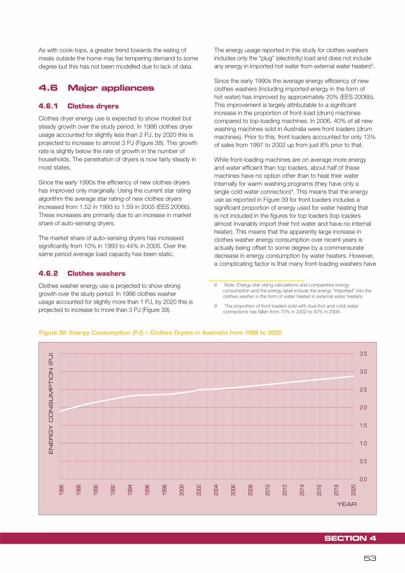
SECTION 4
53
As with cook-tops, a greater trend towards the eating of meals outside the home may be tempering demand to some degree but this has not been modelled due to lack of data.
Major appliances4.6
Clothes dryers4.6.1
Clothes dryer energy use is expected to show modest but steady growth over the study period. In 1986 clothes dryer usage accounted for slightly less than 2 PJ, by 2020 this is projected to increase to almost 3 PJ (Figure 38). This growth rate is slightly below the rate of growth in the number of households. The penetration of dryers is now fairly steady in most states.
Since the early 1990s the efficiency of new clothes dryers has improved only marginally. Using the current star rating algorithm the average star rating of new clothes dryers increased from 1.52 in 1993 to 1.59 in 2005 (EES 2006b). These increases are primarily due to an increase in market share of auto-sensing dryers.
The market share of auto-sensing dryers has increased significantly from 10% in 1993 to 44% in 2005. Over the same period average load capacity has been static.
Clothes washers 4.6.2
Clothes washer energy use is projected to show strong growth over the study period. In 1986 clothes washer usage accounted for slightly more than 1 PJ, by 2020 this is projected to increase to more than 3 PJ (Figure 39).
The energy usage reported in this study for clothes washers includes only the “plug” (electricity) load and does not include any energy in imported hot water from external water heaters8.
Since the early 1990s the average energy efficiency of new clothes washers (including imported energy in the form of hot water) has improved by approximately 20% (EES 2006b). This improvement is largely attributable to a significant increase in the proportion of front-load (drum) machines compared to top-loading machines. In 2006, 40% of all new washing machines sold in Australia were front loaders (drum machines). Prior to this, front loaders accounted for only 13% of sales from 1997 to 2002 up from just 8% prior to that.
While front-loading machines are on average more energy and water efficient than top loaders, about half of these machines have no option other than to heat their water internally for warm washing programs (they have only a single cold water connection)9. This means that the energy use as reported in Figure 39 for front loaders includes a significant proportion of energy used for water heating that is not included in the figures for top loaders (top loaders almost invariably import their hot water and have no internal heater). This means that the apparently large increase in clothes washer energy consumption over recent years is actually being offset to some degree by a commensurate decrease in energy consumption by water heaters. However, a complicating factor is that many front-loading washers have
8 Note: Energy star rating calculations and comparative energy consumption and the energy label include the energy “imported” into the clothes washer in the form of water heated in external water heaters.
9 The proportion of front loaders sold with dual (hot and cold) water connections has fallen from 70% in 2002 to 50% in 2006.
Figure 38: Energy Consumption (PJ) – Clothes Dryers in Australia from 1986 to 2020
0.0
0.5
1.0
1.5
2.0
2.5
3.0
3.5
1986
1988
1990
1992
1994
1996
1998
2000
2002
2004
2006
2008
2010
2012
2014
2016
2018
2020
YEAR
EN
ER
GY C
ON
SU
MPTIO
N (PJ)

RESULTS BY END USE
54
no option for the user to select a true “cold wash” program. That is, they have no program options that do not include at least some degree of internal water heating (often to 30oC is the coldest temperature program available). This is an unfortunate development given the historical popularity of cold washing in Australian households (approximately 70% of washes (ABS4602) (refer also to Section 6 for more details).
Dishwashers4.6.3
Dishwasher energy use is projected to show strong growth over the study period. In 1986 clothes washer usage accounted for slightly more than 1 PJ, by 2020 this is projected to increase to approximately 3 PJ (Figure 40).
Since the early 1990s the average energy and water consumption of new dishwashers has decreased by 40% (EES 2006b). These improvements in efficiency have however been more than offset by a significant increase in the number of households, together with a steady and ongoing increase in ownership of dishwashers.
Ownership since 1986 (19.8%) had more than doubled by 2005 (41.5%) and this is further expected to increase to more than 60% by 2020. Further efficiency gains over the coming years to 2020 are expected to be modest, hence a continued strong growth in energy use is projected.
Refrigerators and freezers4.6.4
Refrigerator and freezer energy use grew slowly at the start of the study period but is now starting to decline. In 1986 refrigerators and freezers usage together accounted for approximately 26 PJ, by 2020 this is projected to have decreased to approximately 24 PJ (Figure 41). This decrease is despite an increase in total stock (refrigerators and freezers) from approximately 10 million units in 1986 to an estimated 17 million units by 2020 (70% increase).
Since the early 1990s the average energy consumption of new refrigerators and freezers has improved significantly, with a 40% reduction from 1993 to 2006 (EES 2006b). These improvements have been driven by both the energy labelling program and by the introduction of MEPS requirements in 1999 followed by more stringent levels in 2005. The 2005 MEPS levels will continue to place downward pressure on energy growth for these products over the study period10.
Microwaves4.6.5
Microwave oven energy use has been growing rapidly since the start of the study period but is now reaching a plateau. In 1986 microwave usage accounted for less than 0.5 PJ, this is estimated to have increased to approximately 2.5 PJ by 2005 and is projected to remain steady until 2020 (Figure 42).
10 Monica Oliphant has observed that “As custom built kitchen ‘makeovers’/renovations increase, refrigerators can become boxed into a small space with poor ventilation. In the absence of regulations for builders and kitchen designers regarding this aspect, significant increases in the energy consumption of these products in the field could be the outcome.”
Figure 39: Energy Consumption (PJ) – Clothes Washers (CW) in Australia from 1986 to 2020
0.0
0.5
1.0
1.5
2.0
2.5
3.0
1986
1988
1990
1992
1994
1996
1998
2000
2002
2004
2006
2008
2010
2012
2014
2016
2018
2020
YEAR
EN
ER
GY C
ON
SU
MPTIO
N (PJ) CW top
CW front

SECTION 4
55
The main drivers for the increase in energy consumption have been, to a lesser extent, the increase in the number of households but more importantly the rapid rise in penetration of microwave ovens. Penetration since 1986 has increased from 30% to 91% in 2005.
Interestingly, about half of the energy consumption of these products is while in standby mode(s). Given that there is limited scope for further growth in ownership likely, the introduction of a standby MEPS (one watt in 2012) is expected to limit projected energy growth from 2005 to 2020 (this is included in the baseline estimates).
Information technology 4.7 products
Computers 4.7.1
Personal computer and laptop energy use has been growing rapidly since the start of the study period but is now slowing to a steady growth rate. In 1986 personal computer and laptop energy usage was negligible, this is estimated to have increased to nearly 3 PJ by 2005 and is projected to continue to rise to almost 6 PJ by 2020 (Figure 43).
The main drivers for the increase in energy consumption have been:
An increase in the number of households, but most importantly the rapid increase in ownership of personal computer and laptops over the study period. Ownership since 1986 (<0.01) had risen to 0.87 for personal
computers and 0.50 for laptops by 2005. Ownership is projected to rise to nominally 1.25 for personal computers and 0.65 for laptops by 2020.
There is some conflicting data regarding computer ownership in homes – some studies put the value at much higher levels.
For personal computers, on mode power consumption has virtually doubled from approximately 50 W to more than 50 W at present. With the advent of more powerful processors, this may continue to rise. But new low-energy variants (driven by demand for use in laptop computers) are now being used in some desktop systems, so future energy trends are not clear. Future labelling and MEPS programs for these products could drive power levels down significantly.
Hours of use have almost doubled since the early 1990s from approximately 500 hours per annum to more than 900 hours per annum. This is projected to continue to rise to approximately 1200 hours per annum by 2020 as they become more ubiquitous and the internet becomes an integral element of education and entertainment in the home.
Future trends in ownership are unclear – values could stabilise near current levels or could increase to as many as 1.5 to two computers per home. This is an area where trend analysis is highly uncertain. Natural energy efficiency improvements (driven by laptop design) and the impact of future programs like MEPS, energy labelling and Energy Star are expected to temper growth in energy use towards the end of the study period (although these programs are not included in the baseline estimates).
Figure 40: Energy Consumption (PJ) – Dishwashers in Australia from 1986 to 2020
0.0
0.5
1.0
1.5
2.0
2.5
3.0
3.5
1986
1988
1990
1992
1994
1996
1998
2000
2002
2004
2006
2008
2010
2012
2014
2016
2018
2020
YEAR
EN
ER
GY C
ON
SU
MPTIO
N (PJ)

RESULTS BY END USE
56
Miscellaneous IT equipment – switched 4.7.2 and unswitched
Miscellaneous Information Technology (IT) equipment energy use has been growing rapidly since the start of the study period. Unswitched equipment energy use has now peaked but switched equipment is expected to continue to grow strongly for the remainder of the study period. In 1986 miscellaneous IT equipment usage was negligible, this is estimated to have increased to nearly 3.5 PJ by 2005 and is projected to continue to double to approximately 7 PJ by 2020 (Figure 44).
The main drivers for the increase in energy consumption have been twofold:
An increase in the number of households but most importantly the rapid increase in ownership of miscellaneous IT equipment. There are currently a total of 3.2 of these devices per computer installed.
Hours of use have almost doubled since the early 1990s from approximately 500 hours per annum to more than 900 hours per annum. This is expected to continue to rise to approximately 1200 hours per annum by 2020. In many homes unswitched equipment (eg broadband connections, routers and switches) are being left in active modes for long periods and while power levels are modest, the energy consumption becomes significant where multiple units are present.
Modest efficiency improvements and the introduction of standby MEPS is not expected to temper much of the growth of unswitched miscellaneous IT equipment energy use.
Switched equipment energy use is expected to remain stable for the remainder of the study period.
Monitors4.7.3
Monitor energy use (used with desktop computers) has been growing rapidly since the start of the study period but is now reaching a plateau with some further growth expected late in the study period. In 1986 monitor energy usage was negligible, this is estimated to have increased to nearly 1.2 PJ by 2005 and is projected to continue to rise (after a small dip around 2012) to almost 1.4 PJ by 2020 (Figure 45).
The main drivers for the increase in energy consumption have been:
The increase in the number of households and strong growth in ownership of monitors (associated with desktop computers) since 1986. Ownership trends are linked to desktop computers.
Hours of use have almost doubled since the early 1990s from approximately 500 hours per annum to more than 900 hours per annum. This is expected to continue to rise to approximately 1200 hours per annum by 2020.
The changeover from CRT to LCD monitors through the period 2000 to 2010 has reduced energy consumption in this period.
Efficiency improvements (particularly following the replacement of CRT with LCD technology) and the impact of the MEPS and EnergyStar could further reduce future energy growth (although these are not assessed).
Figure 41: Energy Consumption (PJ) – Refrigerators/Freezers in Australia from 1986 to 2020
0.0
5.0
10.0
15.0
20.0
25.0
1986
1988
1990
1992
1994
1996
1998
2000
2002
2004
2006
2008
2010
2012
2014
2016
2018
2020
YEAR
EN
ER
GY C
ON
SU
MPTIO
N (PJ) RF
FZ

SECTION 4
57
Figure 42: Energy Consumption (PJ) – Microwaves in Australia from 1986 to 2020
0.0
0.5
1.0
1.5
2.0
2.5
3.0
1986
1988
1990
1992
1994
1996
1998
2000
2002
2004
2006
2008
2010
2012
2014
2016
2018
2020
YEAR
EN
ER
GY C
ON
SU
MPTIO
N (PJ)
Home entertainment 4.8 equipment
DVD, VCR and combination units4.8.1
VCR energy use showed rapid growth since the start of the study period but plateaued off in the mid 1990s following the introduction of DVD technology. In 1986 VCR energy usage was approximately 0.7 PJ, this is estimated to have increased to nearly 1.2 PJ by the mid 1990s but has been in decline ever since and is projected to fall to approximately 0.1 PJ by 2020 (Figure 46).
DVD energy use has shown rapid growth since their introduction in the mid 1990s but is now plateauing off. Commencing in the mid 1990s DVD energy usage is estimated to have risen to approximately 0.6 PJ by 2005 but is now projected to fall to approximately 0.45 PJ by 2020.
The main drivers for the increase in energy consumption by DVDs up until the present time have been twofold:
The rise and fall of ownership for VCRs is driving their energy consumption. The rapid increase in DVD ownership was also the main driver for their increase in energy consumption. Penetration of DVDs since 1995 (0%) had risen to 72% by 2005. Penetration is projected to rise to nominally 97% by 2020 (when ownership is projected to be 1.25 per household).
Hours of use have significantly increased since the mid 1990s from approximately 250 hours per annum to almost 400 hours per annum at present. This is expected to continue to rise to approximately 500 hours per annum by
2020. However, for both of these products their standby modes dominate the energy consumption and the one watt targets will reduce energy consumption in the long term.
The introduction of standby MEPS is expected to result in a projected fall in energy use for DVDs over the coming years until 2020. VCRs will have mostly disappeared by 2020.
Home entertainment – other4.8.2
Home entertainment-other includes mostly stereo components such as amplifiers, CD players, tuners, tape players, integrated and portable stereos etc.
Home entertainment-other energy use had shown rapid growth since the start of the study period but has now plateaued off. In 1986 home entertainment-other energy usage was approximately 0.5 PJ, this is estimated to have now increased to nearly 3.5 PJ but is projected to decline to approximately 2.0 PJ by 2020 (Figure 47).
Limited scope for growth in ownership coupled with the introduction of a standby MEPS in 2012 is driving the projected decline in energy usage from this end use for the remainder of the study period. Again, most of the energy consumption for these products is in standby and related low power modes. It is estimated that there are nearly four of these products per home.

RESULTS BY END USE
58
Games consoles4.8.3
Games console energy use has been growing rapidly since the start of the study period. In 1986 games console energy usage was negligible, this is estimated to have increased to just over 0.2 PJ by 2005 and is projected to continue to rise to just over 1.2 PJ by 2020 (Figure 48).
The main drivers for the increase in energy consumption have been threefold:
The increase in the number of households and the rise in ownership of games consoles. Ownership since 1986 (2%) had risen to approximately 30% by 2005. Ownership is projected to rise to nominally 45% by 2020.
On mode power consumption has increased from approximately 15 W in the 1990s to approximately 50 W by 2005 with a projected 120 W by 2020. Some of the newest and most popular models have very poor on mode energy consumption (150 W).
Standby power consumption has increased from approximately 14 W in the 1990s to approximately 43 W by 2005 with a projected 105 W by 2020. Fortunately most games consoles are either left in off mode or are disconnected when not in use.
Continued growth in penetration combined with significant increases in on mode and standby power consumption could result in continued strong growth in energy usage for games consoles throughout the study period.
Set-top boxes 4.8.4
Set-top boxes are broken into Pay television types (subscription) and free-to-air digital converters to allow the use of legacy analogue televisions with the digital free-to-air broadcasts.
Pay TV set-top box energy use has shown steady growth since their introduction in the mid 1990s but is now plateauing off. In 1995 Pay TV set-top box energy use was negligible, this is estimated to have increased to approximately 0.5 PJ by 2005 a level it is expected to maintain to 2020 (Figure 49).
Free-to-air TV set-top box energy use has shown extremely rapid growth since their introduction at the end of the 1990s but is expected to plateau around 2012. In 2000, free-to-air TV set-top box energy usage was negligible, this is estimated to have increased to approximately 0.5 PJ by 2005 and is expected to continue to grow to almost 2.5 PJ by 2012 after which it is projected to decline to less than 1.5 PJ by 2020.
The key driver for increasing energy use over the past 10 years has been the rapid uptake of these technologies. Pay TV set-top box penetration has risen steadily from nil to approximately 20% in 2005, this is projected to continue to rise to just over 30% by 2020. The growth in ownership of free-to-air set-top boxes is expected to be more prolific growing from nil in 2000 to a projected 0.88 peak around 2012 (penetration 76%). Pay TV set-top boxes are expected to improve in efficiency in the coming years.
0.0
1.0
2.0
3.0
4.0
5.0
6.0
7.0
1986
1988
1990
1992
1994
1996
1998
2000
2002
2004
2006
2008
2010
2012
2014
2016
2018
2020
YEAR
EN
ER
GY C
ON
SU
MPTIO
N (PJ) PC
Laptops
Figure 43: Energy Consumption (PJ) – Computers in Australia from 1986 to 2020

SECTION 4
59
Figure 45: Energy Consumption (PJ) – Monitors in Australia from 1986 to 2020
0.0
1.0
2.0
3.0
4.0
5.0
6.0
7.0
1986
1988
1990
1992
1994
1996
1998
2000
2002
2004
2006
2008
2010
2012
2014
2016
2018
2020
YEAR
EN
ER
GY C
ON
SU
MPTIO
N (PJ) Misc. ITS
Misc. ITU
Figure 44: Energy Consumption (PJ) – Miscellaneous IT in Australia from 1986 to 2020
0.0
0.2
0.4
0.6
0.8
1.0
1.2
1.4
1.6
1986
1988
1990
1992
1994
1996
1998
2000
2002
2004
2006
2008
2010
2012
2014
2016
2018
2020
YEAR
EN
ER
GY C
ON
SU
MPTIO
N (PJ)

RESULTS BY END USE
60
Figure 47: Energy Consumption (PJ) – Home Entertainment in Australia from 1986 to 2020
0.0
0.5
1.0
1.5
2.0
2.5
3.0
3.5
4.0
1986
1988
1990
1992
1994
1996
1998
2000
2002
2004
2006
2008
2010
2012
2014
2016
2018
2020
YEAR
EN
ER
GY C
ON
SU
MPTIO
N (PJ)
Figure 46: Energy Consumption (PJ) – DVD and VCR in Australia from 1986 to 2020
0.0
0.2
0.4
0.6
0.8
1.0
1.2
1.4
1986
1988
1990
1992
1994
1996
1998
2000
2002
2004
2006
2008
2010
2012
2014
2016
2018
2020
YEAR
EN
ER
GY C
ON
SU
MPTIO
N (PJ) DVD
VCR

SECTION 4
61
Beyond 2012, free-to-air set-top box ownership is expected to decline as most new TVs now being supplied with integrated digital tuners. This trend, along with the introduction of MEPS in all modes will significantly reduce the energy consumption associated with this end use (these programs have been included in the estimates). It must be noted that the projected take up of free-to-air digital set-top boxes (converters) is highly uncertain at this stage. DVD recorders with integrated digital tuners are now replacing the functions of VCRs and digital converter set-top boxes. Given that there are some 15 million analogue televisions in the stock at the moment, the take-up rate of these products will be dependent on how many televisions are retired by 2012, the prevalence of TVs with integrated digital tuners by that date and prevalence of other products that could perform the same function as a set top box (other products with a digital tuner that can be shared). All of these factors make the energy projections for this product somewhat uncertain.
Televisions4.8.5
Television energy use has been growing steadily since the start of the study period but is now projected to grow much more rapidly over the remainder of the study period. In 1986 TV usage accounted for approximately 3 PJ, by 2005 this is estimated to have increased to approximately 12 PJ in 2005 and is projected to exceed 45 PJ by 2020 (Figure 50).
The main drivers for the projected rapid increase in energy consumption are:
Penetration of TVs has been above 98% throughout the entire study period, however ownership has been rising with the average number of TVs per household increasing from approximately 1.5 in 1986 to a projected 2.1 by 2020. This effect, combined with increases in household numbers has resulted in a significant increase in stock levels. One in four households buy a new television each year (current sales of about two million units per annum).
Hours of viewing have been rising steadily over the study period from approximately 1500 per annum in 1986 to a projected 2800 hours by 2020 per TV. However, this data is based on limited end-use measurements and there are some uncertainties associated with it.
Since the late 1990s new technologies such as plasma, projection and particularly LCD’s have been gaining market share in favour of CRT, which until 2000 accounted for nearly all new televisions. By 2005 CRT screens accounted for 75% of all sales but by 2007 this is estimated to have fallen to less than 40%. LCDs are projected to have a 70% market share by 2010. All of these newer technologies have are driving a trend towards larger screen sizes. This trend has resulted in a rapid rise in energy consumption from an average on mode consumption of approximately 65W in 1986 to 100 W in 2005 and continuing to grow to an estimated 230 W by 2020. This threefold increase in power consumption, together with increases in hours of operation and increases in ownership is a major driver of increased energy consumption by TVs.
Figure 48: Energy Consumption (PJ) – Games Consoles in Australia from 1986 to 2020
0.0
0.2
0.4
0.6
0.8
1.0
1.2
1.4
1986
1988
1990
1992
1994
1996
1998
2000
2002
2004
2006
2008
2010
2012
2014
2016
2018
2020
YEAR
EN
ER
GY C
ON
SU
MPTIO
N (PJ)

RESULTS BY END USE
62
Active standby power consumption is expected to decline from an average of approximately five watts in the 1990s to less than one watt by 2020. This reduction is being driven by existing trends among manufacturers to reduce standby power consumption along with the one W standby target to be introduced in 2012. These modest savings are however dwarfed by the increases noted above. Energy labelling and MEPS may reduce future energy demand for televisions and the impacts have not been included in the baseline estimates.
Other equipment4.9
Electric kettles4.9.1
Electric kettle use has been growing modestly since the start of the study period. In 1986 electric kettle used 2 PJ of energy consumption, and was estimated to have increased to approximately 2.5 PJ by 2005 with projections to continue to rise to almost 3 PJ by 2020 (Figure 51).
With an estimated steady saturation of one kettle per household and little if any scope for efficiency improvement, electric kettles are expected to maintain a steady but modest growth in line with population growth throughout the study period.
Lighting4.9.2
Lighting energy use has shown steady and relatively strong growth since the start of the study period but is expected to
decline from 2010 to 2015 then begin to rise again for the remainder of the study period. In 1986 lighting energy usage was approximately 13 PJ and by 2005 this is estimated to have increased to nearly 25 PJ with a peak of just over 27 PJ expected in 2010. Following a dip in energy consumption post 2010, consumption is projected to rise again to approximately 25 PJ by 2020 (Figure 52).
Apart from the growth in the number of households and the increase in floor areas of those households, the main drivers influencing the general upward trend in lighting energy consumption are as follows:
Since the early 1990s there has been a strong growth in the use of quartz halogen (QH) lighting. While this type of lighting is slightly more efficient than standard incandescent lighting by a factor of 1.5 to two (approximately 15-20 lumens/watt compared to 10 lumens/watt) it is usually installed with a much higher lumen density (typically more than three times the lighting levels in lumens/m2). This results in a substantial increase in energy consumption.
Compact fluorescent lamps have been slowly gaining market share since their introduction in the late 1980s. The penetration of this relatively efficient technology (approximately 50-65 lumens/watt) is expected to increase rapidly with the announced phase out of incandescent lamps in 2009. This is expected to drive lighting energy consumption downwards for the following five years.
Beyond 2015 it is expected that practically all standard incandescent lamps will have been removed from the stock (largely replaced by CFLs). Beyond 2015 increases in household numbers and the expected continuing
Figure 49: Energy Consumption (PJ) – Set-top Boxes in Australia from 1986 to 2020
0.0
0.5
1.0
1.5
2.0
2.5
3.0
1986
1988
1990
1992
1994
1996
1998
2000
2002
2004
2006
2008
2010
2012
2014
2016
2018
2020
YEAR
EN
ER
GY C
ON
SU
MPTIO
N (PJ) STB FTA
STB PAY

SECTION 4
63
popularity of QH lamps is projected to drive energy consumption upwards again.
At this stage new technologies which may provide a viable high efficiency replacement for QH (possibly fluorescent or LED technology) appear likely, but these have not been factored into the baseline estimates as a timetable for their commercial viability is not known at this stage. Note that linear fluorescent lamps and their ballasts are already subjected to MEPS but these technologies are not prevalent in the residential sector (despite their superior efficiency).
Other electricity (small miscellaneous 4.9.3 loads)
Small miscellaneous loads include power tools, fish tanks, vacuum cleaners, small kitchen appliances (those not normally on standby), pumps, portable or plug based lamps (eg desk lamps or night lights), electric blankets, range-hoods, irons and so forth.
Small miscellaneous load energy use has been growing steadily since the start of the study period, basically in line with the growth of household numbers. In 1986 miscellaneous energy accounted for an estimated 5 PJ of energy consumption, this is estimated to have increased to approximately 7 PJ by 2005 and is projected to continue to rise to approximately 8.5 PJ by 2020 (Figure 53).
Other standby4.9.4
Other standby includes all equipment types that were not explicitly modelled as a separate appliance or product as part of the stock model but that used some power when connected to the mains. A list of the types of products covered can be found in Section 6.6.8.5.
Other standby energy use has been growing rapidly since the mid 1990s. In 1986 other standby energy usage accounted for less than 0.5 PJ of energy consumption, this is estimated to have increased to approximately 8 PJ by 2005 and is projected to continue to rise to more than 18 PJ by 2020 (Figure 54). This growth is despite many of these products having their energy reduced under the one watt MEPS standby requirements in 2012.
Swimming pools and spas4.9.5
Swimming pool energy use in the form of electricity for pumping applications and some heating and gas used for heating has been growing in line with ownership trends over the study period. From the mid 1980s to the mid 1990s ownership was basically static. From the mid 1990s ownership began to rise again slightly and this trend is projected to continue to the end of the study period. No significant improvements in efficiency have been factored in to the estimates.
In 1986 pool and spa energy usage accounted for approximately 6 PJ of energy consumption (electricity approximately 4.5 PJ and gas approximately 1.5 PJ), this is estimated to have increased to approximately 8.5 PJ by 2005 (electricity approximately 6.3 PJ and gas approximately 2.2 PJ) and is projected to continue to rise to more than 11 PJ by 2020 (electricity approximately 8 PJ and gas slightly more than 3 PJ) (Figure 55).
Water beds4.9.6
Water bed energy use (ie resistive electric heating) had shown modest growth from 1986 to the end of the 1990s. Beyond the 1990s, energy use by water beds has been in decline in line with ownership trends. In 1986 water bed energy usage was approximately 1.2 PJ, this is estimated to have peaked at approximately 1.4 PJ by the end of the 1990s and is projected to decline to less than 0.6 PJ by 2020 (Figure 56). The energy consumption per bed is assumed to be constant and the energy consumption tracks ownership (which is based on interpolated ABS data and has not been smoothed).

RESULTS BY END USE
64
Table 51: Energy Consumption (PJ) – Electric Kettles In Australia From 1986 to 2020
0.0
0.5
1.0
1.5
2.0
2.5
3.0
3.5
4.0
4.5
5.0
1986
1988
1990
1992
1994
1996
1998
2000
2002
2004
2006
2008
2010
2012
2014
2016
2018
2020
YEAR
EN
ER
GY C
ON
SU
MPTIO
N (PJ)
Figure 50: Energy Consumption (PJ) – Televisions in Australia from 1986 to 2020
0
5
10
15
20
25
30
35
40
45
50
1986
1988
1990
1992
1994
1996
1998
2000
2002
2004
2006
2008
2010
2012
2014
2016
2018
2020
YEAR
EN
ER
GY C
ON
SU
MPTIO
N (PJ)
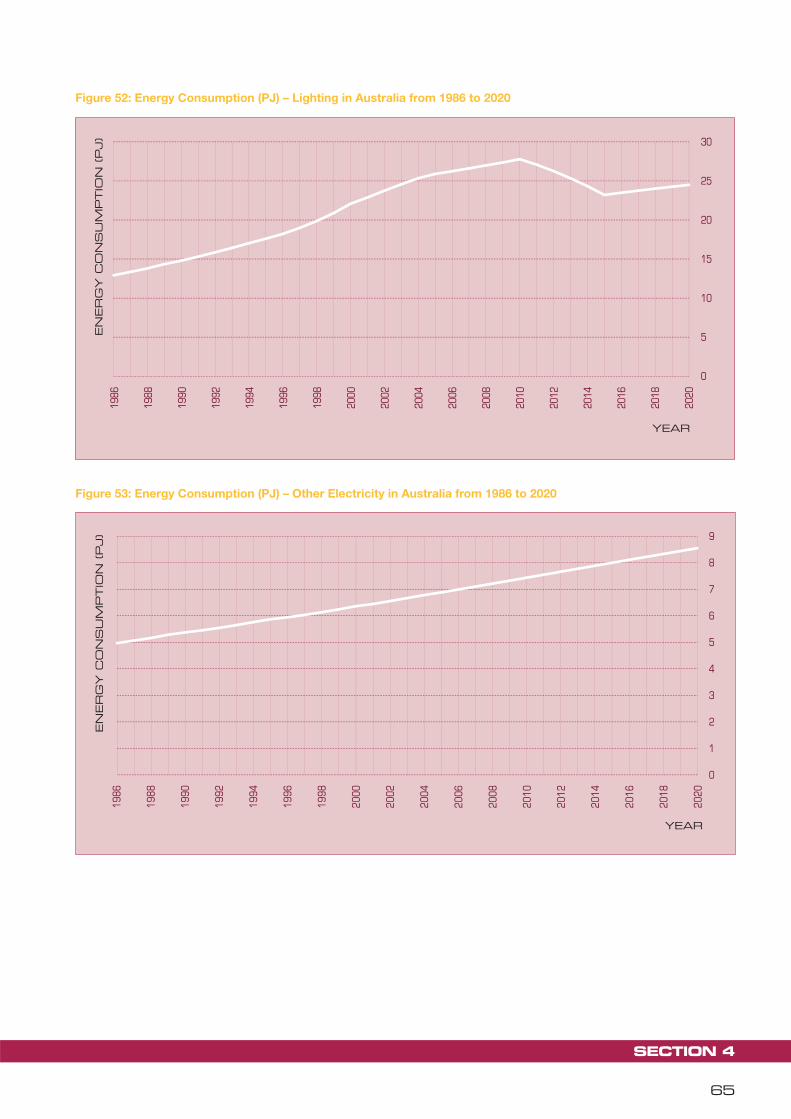
SECTION 4
65
Figure 52: Energy Consumption (PJ) – Lighting in Australia from 1986 to 2020
Figure 53: Energy Consumption (PJ) – Other Electricity in Australia from 1986 to 2020
0
5
10
15
20
25
30
1986
1988
1990
1992
1994
1996
1998
2000
2002
2004
2006
2008
2010
2012
2014
2016
2018
2020
YEAR
EN
ER
GY C
ON
SU
MPTIO
N (PJ)
0
1
2
3
4
5
6
7
8
9
1986
1988
1990
1992
1994
1996
1998
2000
2002
2004
2006
2008
2010
2012
2014
2016
2018
2020
YEAR
EN
ER
GY C
ON
SU
MPTIO
N (PJ)

RESULTS BY END USE
66
Figure 55: Energy Consumption (PJ) – Swimming Pools in Australia from 1986 to 2020
0
1
2
3
4
5
6
7
8
9
1986
1988
1990
1992
1994
1996
1998
2000
2002
2004
2006
2008
2010
2012
2014
2016
2018
2020
EN
ER
GY C
ON
SU
MPTIO
N (PJ) Electricity
Gas
YEAR
Figure 54: Energy Consumption (PJ) – Other Standby in Australia from 1986 to 2020
0
2
4
6
8
10
12
14
16
18
20
1986
1988
1990
1992
1994
1996
1998
2000
2002
2004
2006
2008
2010
2012
2014
2016
2018
2020
YEAR
EN
ER
GY C
ON
SU
MPTIO
N (PJ)

SECTION 4
67
Figure 56: Energy Consumption (PJ) – Water Beds in Australia from 1986 to 2020
0.0
0.2
0.4
0.6
0.8
1.0
1.2
1.4
1.6
1986
1988
1990
1992
1994
1996
1998
2000
2002
2004
2006
2008
2010
2012
2014
2016
2018
2020
YEAR
EN
ER
GY C
ON
SU
MPTIO
N (PJ)

68

POPULATION AND HOUSEHOLD ESTIMATES
SECTION 5

POPULATION AND HOUSEHOLD ESTIMATES
70
POPULATION AND 5 HOUSEHOLD ESTIMATES
Overview of estimates5.1 It is always difficult to get a consistent time series for household numbers and population in the residential sector. Historical data from ABS is mainly based on census data. However, the census value for households is always adjusted slightly to correct for missing data, visitors and people who are travelling and so forth.
Before documenting the estimates used in this report, it is useful to review the mains terms used.
Estimated Resident Population (ERP): These are estimates of the Australian population obtained by adding to the estimated population at the beginning of a period, the components of natural increase (on a usual residence basis) and net overseas migration less deaths. For states and territories, account is also taken of estimated interstate movements involving a change of usual residence. After each census, ABS usually makes estimates for the preceding inter-censual period by incorporating additional data obtained from the new census plus a range of other surveys conducted during this period. The estimates of ERP are based on adjusted census counts (which tend to under enumerate population) by place of usual residence, to which the number of Australian residents estimated to be temporarily overseas at the time of census. ERP is the key variable in terms of estimating population for modelling purposes. Note that overseas visitors were not included. The concept of ERP links people to a place of usual residence within Australia. Usual residence is that place where each person has lived or intends to live for six months or more in the reference year. Estimates of ERP are available from 1971.
Households: The definition of a household used by the Australian Bureau of Statistics (ABS) in its appliance surveys is “a group of persons who are the usual residents of a dwelling and who have some common provision for food and other housekeeping arrangements” (ABS8218.0).
One source of historical source of data for households was the Australian Bureau of Statistics Census of Population and Housing, which has been held at five-yearly intervals since 1961. Household types listed in the census include private, non-private (hotels, institutions, barracks, staff quarters etc) and unoccupied. This study is based on values for occupied private households. Prior to 1986, caravans were counted as non-private dwellings, but from 1986, they have been included as private occupied dwellings. The census also generally gives some limited information on the dwelling structure.
A dwelling is a building or structure in which people live. This can be a building such as a house, part of a building such as a flat, or it can be a caravan or even a tent. Houses under construction, derelict houses or converted garages are not counted as dwellings in the census.
A private dwelling is normally a house, flat or even a room, but it can also be a house or rooms attached to shops or offices. Private dwellings can be either occupied or non-occupied. This study has excluded non-occupied private dwellings. Occupied private dwellings can have more than one household, but this is fairly unusual in Australia, so households are seen as a proxy for dwellings.
Non-private dwellings are those dwellings not included in private dwellings, which provide a communal or transitory type of accommodation. These dwellings include hotels, motels, guest houses, prisons, religious and charitable institutions, defence establishments, residential parts of educational institutions, hospitals (including staff accommodation) and other communal dwellings. For this study, non-private dwellings have been excluded from the household estimates. These are generally associated with commercial sector energy consumption and include such things as prisons, hospitals and residential accommodation in commercial buildings. This study covers all households which live in Class one and two buildings as defined under the building Code of Australia.
Estimates used for this 5.2 study
For the original baseline study (EES 1999), the only household estimates available were from historical surveys (such as ABS8212 and ABS4602) and census estimates. For the 1999 study projections of household numbers used population projections from ABS3222.0 together with trend data on household sizes to provide an estimate of future household numbers.
In June 2004, ABS for the first time released projections of households at a state level to 2026 in its report Household and Family Projections (ABS3236.0). This study provides an integrated projection of households and population at a state level.
While population forecasts are also available in ABS3222.0, the ERP and household figures in ABS3236 have been used to ensure a consistent data set for historical and projected household numbers. ABS3236 has three projection series as follows:

SECTION 5
71
Series I – No change in propensities. Living arrangement propensities for 2001 remain constant to 2026.
Series II – Low rate of change in propensities. The linear trend in propensities from 1986 to 2001 continues at the full rate of change to 2006, half the rate of change to 2011, one-quarter the rate of change to 2016, and then remains constant to 2026.
Series III – Continuation of 1986 to 2001 rate of change in propensities. The linear trend in propensities from 1986 to 2001 continues at the full rate of change to 2026.
Propensities are essentially the proportion of the population broken down by five-year age groups and by living arrangements (such as couple with children, couple without children, one parent family, other families, group households, lone persons). The trends in these propensities were examined from census data in 1986 to 2001 and trends established and household estimates generated within the bounds of the projected ERP to 2021. Series III has been used for modelling in this report (continuation of current trends in the main propensities) as this appears to be the most realistic in terms of future household projections.
For data prior to 2001, the ABS has published some historical household data in ABS3101 which gives data on ERP and household estimates from 1991-2001 after adjustments to take into account census data. Unfortunately, the ABS3101 data appears to have some inconsistencies (some large state variability from year-to-year).
Prior to 1991, census data for households was used together with linear interpolation between census surveys. These census values were adjusted by the relevant adjustment factors at a state level to get consistent data between ABS3101 values and the overlapping census values.
Some small adjustments to the resulting ABS data for the period 1986 to 2006 have been made in order to smooth state variations from year-to-year and to better match known new housing approvals from ABS building approval data obtained from local councils. Details of these adjustments are set out in Section 7.
A table of the household numbers and the population by year and state are set out in Table 10.

POPULATION AND HOUSEHOLD ESTIMATES
72
Table 10: Estimated Number of Occupied Residential Households (‘000s)
Year NSW VIC QLD SA WA TAS NT ACT AUS
1990 2,072 1,544 1,030 537 564 172 47 94 6,060
1991 2,100 1,560 1,059 546 575 175 48 96 6,160
1992 2,133 1,578 1,097 554 588 178 50 99 6,277
1993 2,171 1,600 1,139 563 605 181 51 103 6,413
1994 2,210 1,624 1,189 571 625 184 52 106 6,562
1995 2,252 1,647 1,229 578 642 186 54 109 6,695
1996 2,283 1,663 1,255 581 653 187 55 110 6,787
1997 2,320 1,685 1,286 585 664 188 56 112 6,896
1998 2,360 1,713 1,319 591 677 189 58 114 7,022
1999 2,400 1,744 1,347 597 693 190 59 116 7,148
2000 2,440 1,784 1,381 605 710 192 60 118 7,290
2001 2,465 1,812 1,404 610 721 192 61 120 7,385
2002 2,503 1,848 1,435 618 736 194 62 122 7,518
2003 2,541 1,883 1,471 626 753 196 63 124 7,656
2004 2,577 1,916 1,510 634 771 198 64 127 7,797
2005 2,605 1,946 1,544 642 789 201 66 128 7,920
2006 2,640 1,972 1,581 647 805 202 68 130 8,045
2007 2,676 1,999 1,619 652 821 203 69 131 8,172
2008 2,711 2,027 1,658 657 837 205 70 133 8,298
2009 2,747 2,054 1,696 663 853 206 71 135 8,425
2010 2,782 2,082 1,734 668 869 207 72 137 8,551
2011 2,817 2,109 1,772 673 885 209 73 138 8,677
2012 2,853 2,137 1,810 678 901 210 75 140 8,803
2013 2,888 2,164 1,848 683 916 212 76 142 8,928
2014 2,923 2,191 1,886 688 932 213 77 143 9,053
2015 2,958 2,218 1,923 694 948 214 78 145 9,178
2016 2,993 2,245 1,961 699 964 216 79 147 9,303
2017 3,028 2,272 1,999 704 979 217 80 149 9,428
2018 3,063 2,299 2,036 709 995 218 81 150 9,552
2019 3,097 2,326 2,074 714 1,011 219 83 152 9,676
2020 3,132 2,353 2,111 719 1,026 221 84 154 9,800