energy transport by acoustic modes of harmonic lattices
TRANSCRIPT

Energy transport by acoustic modes of harmonic
lattices
Lisa Harris∗, Jani Lukkarinen†, Stefan Teufel‡, and Florian Theil∗
November 20, 2006
Abstract
We study the large scale evolution of a scalar lattice excitation u whichsatisfies a discrete wave-equation in three dimensions, ut(γ) = −∑
γ′ α(γ −γ′)ut(γ
′), where γ, γ ′ ∈ Z3 are lattice sites. We assume that the dispersion
relation ω associated to the elastic coupling constants α(γ − γ ′) is acoustic,i.e., it has a singularity of the type |k| near the vanishing wave vector, k = 0.
To derive equations that describe the macroscopic energy transport weintroduce the Wigner transform and change variables so that the spatialand temporal scales are of the order of ε. In the continuum limit, which isachieved by sending the parameter ε to 0, the Wigner transform disintegratesinto three different limit objects: the transform of the weak limit, the H-measure and the Wigner-measure. We demonstrate that these three limitobjects satisfy a set of decoupled transport equations: a wave-equation forthe weak limit of the rescaled initial data, a dispersive transport equationfor the regular limiting Wigner measure, and a geometric optics transportequation for the H-measure limit of the initial data concentrating to k = 0.
A simple consequence of our result is the complete characterization ofenergy transport in harmonic lattices with acoustic dispersion relations.
1 Introduction.
The energy transport by atomistic oscillations in crystalline solids is a centralquestion in solid state physics. To the first order approximation, the oscillations
∗Warwick University, Mathematics Institute, Coventry, CV4 7AL, UK†Zentrum Mathematik, Technische Universitat Munchen, Boltzmannstr. 3, D-85747 Garch-
ing, Germany‡Mathematisches Institut, Auf der Morgenstelle 10, 72076 Tubingen, Germany
1
can be described by a discrete wave equation
ut(γ) = −∑
γ′
α(γ − γ′)ut(γ′)
where u(γ) ∈ R is composed out of the displacements of the crystal atoms fromtheir equilibrium position, as will be discussed in Sec. 1.1. Solutions of the dis-crete wave equation preserve the Hamiltonian H(u, u) which is defined in equation(2.2). To analyze physically relevant properties of the crystal, such as its thermalconductivity, we first need to understand how energy is transported within thecrystal via purely harmonic vibrations. Such transport properties are determinedby the dispersion relation ω of the crystal, here ω(k) =
√
α(k), the “hat” denotinga discrete Fourier transform. If ω is not smooth, then depending on the wavelengthdifferent types of continuum energy transport equations can arise. We follow thebasic ideas of Luc Tartar who developed in the 1980s a mathematical frameworkthat can be used to analyze the weak limits of certain nonlinear quantities, theenergy density being one of them.
Our main interest is to characterize the macroscopic evolution of the energydensity. The starting point of our mathematical analysis is the Wigner transformwhich can be interpreted as a “wavenumber resolved” energy density. Let us leavethe details for Sec. 2.1, and only summarize the main findings here. The Wignertransform W ε = W ε[ψ] of the field ψ ∈ `2(Z
3) corresponding to a given normalmode allows defining the corresponding energy density, eε = eε[ψ], by the formula
eε(x) =
∫
T3
dkW ε(x, k), (1.1)
where ε > 0 denotes the “lattice spacing” and x ∈ R3 is a variable which interpo-lates between the points on the scaled lattice εZ3. Here T3 denotes the 3-torus,and we identify T
3 = R3/Z3. Thanks to the equality
∫
R3 dq∫
T3 dkW ε(x, k) =H(ut=0, ut=0) we are able to identify eε(x) as the energy density at position x ∈ Rd.
A limit of a sequence (W ε[ψε]), where ε tends to 0, is in general given by anon-negative Radon-measure µ ∈M+. For such limit measures to form a sensibleapproximation for the original dynamical system, the convergence property needsto be retained in the time-evolution. In addition, for such a description to beuseful, µt should also satisfy an autonomous evolution equation. However, this istypically not possible if the initial measure concentrates to the singular set of ω,i.e., to the points where ω is not smooth. Here we will augment the above Wignertransform scheme to encompass the most common type of singularity encounteredin solid state physics: the case when ω behaves like |k| near k = 0. Such modeswill occur in general within crystal models with short range interactions, andthey are particularly important as they are responsible for sound propagation in
2
the crystal. With some effort, it is likely that our results could be extended tocover any dispersion relation for which the singular set consists of isolated points.However, we will not explicitly spell out the general result here.
Our result can be seen as a generalization of the analysis in [1] where it is shownthat µt can be computed from µ0 by solving a dispersive linear transport equationprovided that µ has no concentrations at wavenumbers k where the dispersionrelation ω is not C1.
If the dispersion relation is not almost everywhere C1 (with respect to the initialWigner-measure), we have to resolve finer details of the asymptotic behavior ofthe sequence of initial conditions. More precisely, we show that if the sequenceof initial excitations is bounded and tight in `2(εZ
3) then for all t ∈ R there aretwo measures, a Wigner-measure µt on R3 ×T3
∗ and an H-measure µHt on R3 ×S2,
and an L2-function φt such that W ε[ψε(t/ε)] converges along a subsequence to(µt, µ
Ht , φt) in a certain weak sense (Theorem 3.2). The subsequence can be chosen
independently of t, and it will only be relevant for determining the limit of theinitial data, that is, (µ0, µ
H0 , φ0). For all other times t ∈ R, the measures µt, µ
Ht
and the L2-function φt can be determined using the transport equations
∂tµt(x, k) + 12π∇ω(k) · ∇xµt(x, k) = 0, k ∈ T
3∗ , (1.2)
∂tµHt (x, q) + 1
2π∇ω0(q) · ∇xµ
Ht (x, q) = 0, q ∈ S2 , (1.3)
∂2t φ = div( 1
(2π)2A0∇φ), (1.4)
together with the initial conditions
µ|t=0 = µ0, µH∣
∣
t=0= µH
0 , φ|t=0 = φ0, ∂tφ(t, q)|t=0 = −iω0(q)φ0(q). (1.5)
Here the constant matrix A0 and the function ω0 are determined by the Hessianof the square of the dispersion relation ω (defined in (2.6)) at k = 0, explicitly
A0 =1
2D2ω2(0), ω0(q) =
√
q · A0q. (1.6)
Equation (1.2) describes the propagation of energy along the harmonic latticewith the group velocity ∇ω(k)/(2π). Equation (1.4) is the wave equation which de-scribes the evolution of macroscopic fluctuations. Equation (1.3) is usually knownunder the name “geometric optics” and it describes the evolution of macroscopicfluctuations whose wavelength is much longer than the lattice spacing ε and muchsmaller than 1, the wavelength of the fluctuations resolved by φ.
It follows easily from our analysis that the sum of the energies of µ, µH and φ isa constant of motion and equals the limiting value of the total energy of the initialexcitations.
3

Standard results in semi-classical analysis show that the Wigner measure µ and∫
R3 dq W 1[φ](x, q) are non-negative. Hence, a key step in our analysis is to demon-strate that also µH has a sign. The measure µH is closely related to the H-measurewhich was introduced by L. Tartar in [2] and P. Gerard in [3], but in general itdiffers from the H-measure.
The Wigner transform, or the Wigner function, was originally introduced tostudy semi-classical behavior in quantum mechanics but it has been proven to bea useful tool in studying large scale behavior of wave equations, as well [4, 5]. Inparticular, the method of calculating continuous, macroscopic energy by findingthe limit object of a sequence of energies eε on rescaled lattice models is one thathas been widely used and justified in, for example, [1, 6, 7]. In [1], the Wignertransform of the normal modes is employed in solving the macroscopic transportof energy in the above harmonic systems for deterministic initial data. The samesystem is considered in [8] with random initial data and in a larger function space,however, excluding the type of concentration effects we study here.
The main use of the Wigner transform is that, unlike the energy density eε itself,it contains enough information so that it satisfies a closed equation in the limitε → 0. Indeed, it was shown in [1] that, as long as there is no concentration onthe singular set of the dispersion relation faster than ε1/2, the Wigner transformof the time-evolved state vector ψ(t/ε) converges to a limit measure µt on R × K.Here K is a suitable compactification of T3 \ S, S = the singular set, which allowsa continuous extension of the group velocity ∇ω. The measure µt is then provento satisfy the transport equation
∂tµt(x, k) + 12π∇ω(k) · ∇xµt(x, k) = 0. (1.7)
It was also shown in [1], that if the weak limit of the rescaled initial data exists,then the limit satisfies the continuum wave equation. However, removing theassumption about the rate of concentration, as well as combining the result witha non-zero weak limit for the initial data remain open questions.
In this paper we will show how to overcome the above difficulties in a physicallyrelevant class of models with a singular dispersion relation. In Section 2 we will firstpresent the microscopic dynamical model in detail. In Section 2.1 we will definethe Wigner transform, and discuss its relation to the energy of the microscopiclattice model. The main results will be presented in Section 3.
1.1 Relation with solid state physics
A crystal in solid state physics is a state of matter in which the atoms retain anearly perfect periodic structure over macroscopic times. The Hamiltonian modelused for the time-evolution in such a crystal is, to the first order accuracy, har-monic. If we assume that each periodic cell of the idealized perfectly periodic
4

crystal structure contains n atoms, then we can form a vector q(γ) ∈ R3n out
of the displacements of the atoms in the periodic cell labeled by γ ∈ Z3. The(classical) Hamiltonian equations of motion of this harmonic model are then
qi(γ, t) =1
mipi(γ, t), pi(γ, t) = −
∑
γ′,i′
A(γ − γ′)i,i′qi′(γ′, t) (1.8)
where γ ∈ Z3, i = 1, . . . , 3n, and mi denotes the mass of the atom whose displace-ment qi measures.
By the change of variables to qi(γ) = m1
2
i qi(γ), pi(γ) = m− 1
2
i pi(γ), these equa-tions can be transformed into a standard form whose force matrix is given byA(γ)i,i′ = m
−1/2i A(γ)i,i′m
−1/2i′ . The standard form equations can then be solved by
Fourier transform, and a diagonalization of the remaining multiplicative evolutionequations decomposes the 3n vector degrees of freedom into independent normalmodes, called phonons in solid state physics. Each normal mode is a complexscalar field on the crystal lattice, and its time-evolution is unitary and uniquelydetermined by the corresponding dispersion relation ωi(k) on T
3. More detailsabout the related mathematical issues can be found in [1, 8].
From the physical perspective it is highly relevant to understand energy trans-port in the case where ω is acoustic in the sense that it contains a |k| singularity.In this case ω is degenerate for large wave-numbers in the sense that the velocityat which long waves propagate converges to the speed of sound. In other words,the energy density can travel ballistically over large distance without experiencingdilution effects due to dispersion.
Acoustic dispersion relations arise in general from atomistic Hamiltonians withshort range harmonic interactions. For instance, for the type of interactions consid-ered in [1] all dispersion relations are Lipschitz continuous and piecewise analytic.In solid state physics, the modes are accordingly divided into optical and acousticdepending on this regularity: if the dispersion relation is regular at k = 0, thenthe mode is called optical, if it behaves as |k| at k = 0, then the mode is calledacoustic. The latter name arises as these modes are believed to be responsible forthe propagation of sound waves in the crystal.
The simplicity of the Fourier-picture is the reason that the dispersion relation isthe starting point of most of the more physically oriented publications. Obviously,within the context of harmonic defect-free crystals both approaches are completelyequivalent. In the beginning of Section 2 we will provide the mathematical detailswhich establish this equivalence on an elementary level.
Finally, let us remark that the discrete linear wave equation alone does not sufficeto determine the physically relevant properties of the crystal, such as its thermalconductivity. However, it forms the basis for perturbative treatments using which
5
these questions can be addressed. We refer to [9, 10, 11] for further details on thephysical aspects of the topic and to [12] for a review about related open problems.
Acknowledgments
We would like to thank Alexander Mielke and Herbert Spohn for several instructivediscussions. JL was supported by the Deutsche Forschungsgemeinschaft (DFG)projects SP 181/19-1 and SP 181/19-2.
2 The microscopic model
There are two mathematically equivalent descriptions of harmonic crystals. On theone hand, one can work with the Hamiltonian equations of motion and analyze theproperties of the solutions. At least formally anharmonic crystals can be discussedin the same way. On the other hand, one can utilize the periodicity and linearityto condense the Hamiltonian into the dispersion relation. While this approach isvery elegant, it cannot be used to directly analyze nonlinear models.
We will show in this chapter how for harmonic lattices the first approach reducesto the second one. Then we demonstrate how the tool of Wigner functions can bebrought to bear on the reduced description.
We assume that the scalar excitation ut(γ), γ ∈ Z3 satisfies the discrete wave
equation∂2
∂t2ut(γ) = −
∑
γ′∈Z3
α(γ − γ′)ut(γ′) (2.1)
with initial data (u|t=0, ∂tu|t=0) ∈ X = `2 × `2. The numbers α(γ − γ′) are theelastic coupling constants between the sites γ and γ ′. We assume that α is real andsymmetric (α(−γ) = α(γ)). Clearly system (2.1) can be written in a Hamiltonianform and the energy
E(u) = H(u, u) =1
2
∑
γ∈Z3
|u(γ)|2 +∑
γ∈Z3
∑
γ′∈Z3
u(γ)α(γ − γ′)u(γ′)
(2.2)
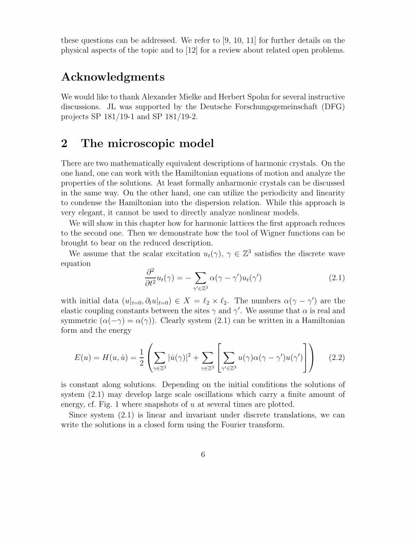
is constant along solutions. Depending on the initial conditions the solutions ofsystem (2.1) may develop large scale oscillations which carry a finite amount ofenergy, cf. Fig. 1 where snapshots of u at several times are plotted.
Since system (2.1) is linear and invariant under discrete translations, we canwrite the solutions in a closed form using the Fourier transform.
6

−60 −40 −20 0 20 40 60
−1
−0.8
−0.6
−0.4
−0.2
0
0.2
0.4
0.6
0.8
1
γ1
z t(γ1,0
)
−60 −40 −20 0 20 40 60−0.015
−0.01
−0.005
0
0.005
0.01
0.015
γ1
−60 −40 −20 0 20 40 60−0.01
−0.008
−0.006
−0.004
−0.002
0
0.002
0.004
0.006
0.008
0.01
γ1
Figure 1: Values of u(γ, t) along the axis γ2 = γ3 = 0 for t = 0, t = 0.1/ε, t = 0.9/εwith ε = 1
7∗10−1. The evolution is given by (2.1) with the nearest neighbor elastic
couplings (2.12), and the initial conditions are ut=0(0) = 1, ut=0(γ) = 0 for allγ 6= 0 and ut=0 ≡ 0.
Definition 2.1 We define the Fourier transform `2(Z3) → L2(T3) by extending
(Fγ→kψ)(k) = ψ(k) =∑
γ∈Z3
e−2πik·γψ(γ) (2.3)
from ψ with finite support to all of `2(Z3). Here T3 = R3/Z3 denotes the unit
3-torus. The inverse transform is pointwise convergently defined by the integral
(Fk→γψ)(γ) =
∫
T3
dk e2πik·γψ(k) = ψ(γ). (2.4)
where the measure dk is induced by the Lebesgue measure on [− 12, 1
2]3. In particular,
∫
T3 dk = 1.
If one applies the Fourier transform to equation (2.1) one obtains the simplersystem
∂
∂t
(
u(k, t)v(k, t)
)
=
(
0 1−ω2(k) 0
) (
u(k, t)v(k, t)
)
. (2.5)
The function ω : T3 → R is the dispersion relation and is related to the atomisticHamiltonian via the following formula
ω(k) =√
α(k) =
√
∑
γ∈Z3
α(γ) cos(2πγ · k). (2.6)
where we have employed the assumption α(γ) = α(−γ). Since α is real andsatisfies the above symmetry property, we find that ω is also real and symmetric,i.e. ω(k) = ω(−k).
7

Now diagonalizing the matrix on the right hand side of (2.5) motivates combiningthe real scalar fields u, v into the two complex fields ψ± = ψ±[u, v] ∈ `2(Z
3,C)defined by the formula
ψσ(k) =1√2
(ω(k)u(k) + iσv(k)) (2.7)
where σ = ±1. For all (u, v) ∈ X, we clearly have ψσ ∈ L2(T3), and thus ψσ ∈`2(Z
3). In addition, since we assumed ω(−k) = ω(k), we also have ψ−(γ) = ψ+(γ)for all γ. The transformation can always be inverted by applying
v = − i√2(ψ+ − ψ−), u =
1
ω√
2(ψ+ + ψ−). (2.8)
These fields are normal modes of the harmonic system, since (2.5) implies thatψ±(γ, t) = ψ±[u(t), v(t)](γ) satisfy the evolution equations
∂
∂t
(
ψ+(k, t)
ψ−(k, t)
)
= −i
(
ω(k) 00 −ω(k)
) (
ψ+(k, t)
ψ−(k, t)
)
, (2.9)
which are readily solved to yield for all t ∈ R, k ∈ R
ψ±(k, t) = e∓iω(k)tψ±(k, 0) . (2.10)
These are exactly the two evolution equations corresponding to a “phonon” modewith a dispersion relation ω.
After these reduction steps it is obvious that the dispersion relation ω fullydetermines the properties of the solutions. We will assume throughout this paperthat ω is of acoustic type in the following precise sense:
Definition 2.2 We call ω ∈ C(T3, [0,∞)) an acoustic dispersion relation if λ =ω2 satisfies:
1. λ ∈ C(3)(T3, [0,∞)).
2. λ(0) = 0, and the Hessian of λ is invertible at 0.
A dispersion relation is called regular acoustic, if it is acoustic and λ(k) > 0 fork 6= 0. The 3 × 3-matrix A0 is the Hessian of 1
2λ at k = 0 and ω0(q) =
√q · A0q.
These assumptions are fairly general: as discussed in the introduction, all stableharmonic interactions have non-negative eigenvalue functions λ, and for interac-tions of the type discussed in [1] ω =
√λ is Lipschitz continuous.
8

A prototype for the kind of dispersion relations we will consider here is thedispersion relation of the nearest neighbor square lattice:
ωnn(k) =[
3∑
ν=1
2(1 − cos(2πkν))]
1
2
. (2.11)
This is clearly a regular acoustic dispersion relation, in the sense of Definition 2.2,and for it A0 is proportional to a unit matrix and ω0(q) = 2π|q|. The correspond-ing elastic couplings are given by αnn(γ
′ − γ) = −∆γ′γ, where ∆ is the discreteLaplacian of the square lattice. Explicitly,
αnn(γ) =
6, if γ = 0,
−1, if |γ| = 1,
0, otherwise.
(2.12)
To allow the creation of macroscopic oscillations we work with sequences of initialconditions that depend on the scaling-parameter ε > 0 and consider the asymptoticbehavior of the solutions as ε tends to 0.
2.1 Energy density and the lattice Wigner transform
From now we will focus on analyzing asymptotic behavior of the fields ψ± as εtends to 0. As is carefully discussed in [1], generalizing the definitions of theenergy density and of the Wigner transform to the discrete setting is not completelyobvious. In an attempt to minimize unnecessary repetition of certain basic resultsrelated to Wigner transforms, we will resort here to the definitions used in [7] whichwill allow us to rely on the properties proven in Appendix B of that reference.However, we wish to keep in mind that this choice might not be optimal for allpurposes, and we refer the interested reader to the discussion and to the referencesin [1, 13] for further possibilities.
We employ here the definition that for any state (u, v), its energy density, eε =eε[u, v], scaled to a lattice spacing ε > 0, is the tempered distribution defined viathe complex fields ψσ = ψσ[u, v] in (2.7):
eε(x) =∑
γ∈Z3
δ(x− εγ)1
2
∑
σ=±1
|ψσ(γ)|2 (2.13)
where δ denotes the Dirac delta-distribution. This is a manifestly positive distri-
9

bution, and identifiable with a measure whose total mass equals the total energy:
∫
dx eε(x) =∑
γ∈Z3
1
2
∑
σ=±1
|ψσ(γ)|2 =1
2
∑
σ=±1
‖ψσ‖2
=1
4
∑
σ=±1
∫
dk |ω(k)u(k) + iσv(k)|2 = H(u, u) <∞. (2.14)
This justifies calling eε an energy density: it defines a distribution of the positivetotal energy between the lattice sites. The symmetry of ω implies that |ψ−(γ)| =|ψ+(γ)| and thus we can also identify the energy density directly with the norm-density of ψ+:
eε(x) =∑
γ∈Z3
δ(x− εγ)|ψ+(γ)|2. (2.15)
Then also for all ε > 0,
H(u, v) =
∫
dx eε(x) = ‖ψ+‖2`2(Z3) = ‖ψ+‖2
L2(T3) = ‖ψ−‖2L2(T3) (2.16)
which is conserved when (u, v) = (u(t), v(t)).
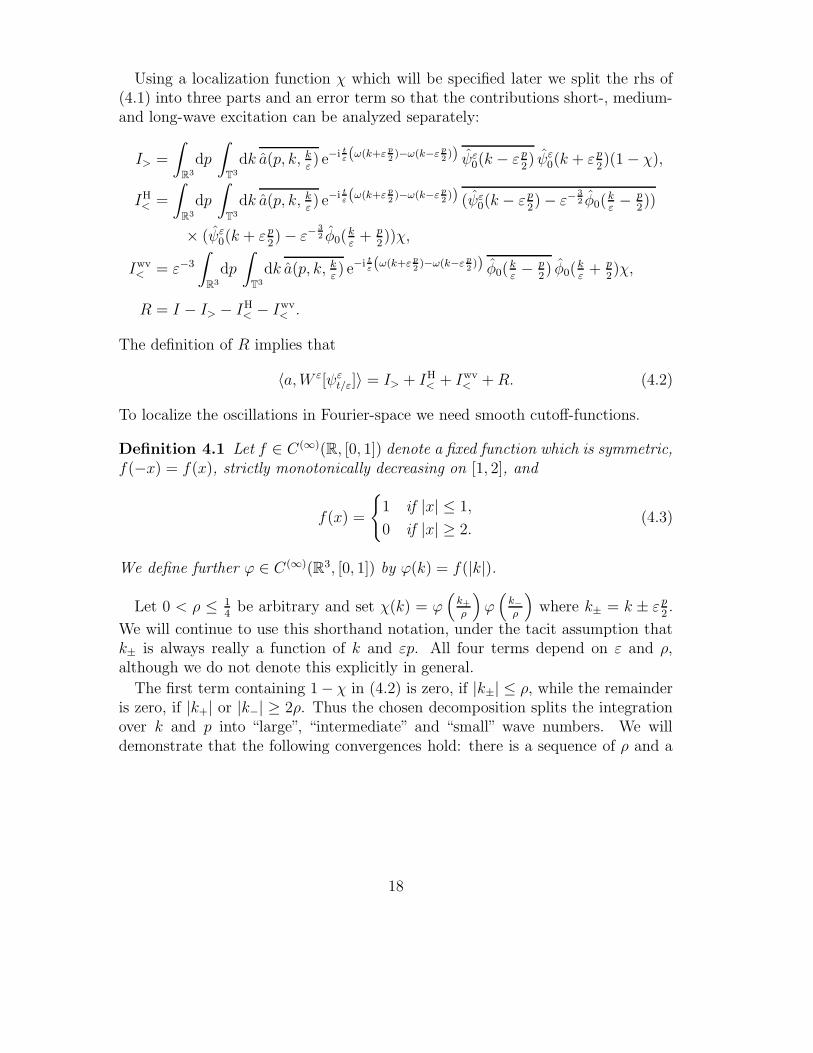
We have given an example of the time-evolution of the so defined energy densityin Fig. 2. The last panel in the figure contains the most obvious features whichare implied by the corresponding macroscopic evolution equation: the points ofdiscontinuity of the solution. The macroscopic initial data is given by µ0(dx, dk) =δ(x)1
2|ω(k)|2dxdk, which has no concentration at k = 0. Thus only (1.2) is relevant.
It is readily solved to yield as the energy density
e(x, t) =
∫
T3
dk δ(x− t 12π∇ω(k)) = t−3
∫
T3
dk δ(xt− 1
2π∇ω(k)) (2.17)
Evaluating such integrals has been considered, for instance, in Sec. 6.4 of [1].|∇ω(k)| has its maximum near the point of discontinuity of the gradient, at k = 0.This defines the outer circle outside which the solution must be zero. Inside thecircle, the solution has a finite density, apart from points which correspond tovalues of k for which the Hessian of ω is not invertible. We have computed thepositions of such points using Mathematica, and plotted the result in the last panelin Fig. 2. For a reader interested in the details of the computation, we point outthat considering the case x3 = 0 simplifies the problem, as it implies that eitherk3 = 0 or k3 = 1
2.
We are interested in the limiting behavior of eε[u(t/ε), u(t/ε)], as ε tends to 0.Since the velocity of the waves with wave vector k depends on k it is necessary to
10

γ1
γ 2
−128 0 128
−128
0
128
γ1
γ 2
−128 0 128
−128
0
128
γ1
γ 2
−128 0 128
−128
0
128
Figure 2: First three panels: Snapshots of the energy density |ψ+(γ, t)|2 in theplane γ3 = 0 at t = 0.1/ε, t = 0.3/ε and t = 0.95/ε, ε = 1
128, with initial data and
elastic constants as in Fig. 1. The plot is of the logarithm of the density, with allvalues less than a fixed cut-off shown white. Last panel: Plot of the restriction tothe plane x3 = 0 of the singular set of the solution to the transport equation (1.2)with the corresponding macroscopic initial data. As the solution is scale-invariant,no explicit length scale has been denoted.
11

work with an object that encodes the density of waves with wave vector k ∈ T3 at
x ∈ R3. This job is conveniently done by the Wigner-transform. In order to avoidcertain technical difficulties we are going to define our Wigner-transform only inthe sense of distributions, i.e., via a duality principle.
First we introduce the space of Schwartz functions.
Definition 2.3 Let Sd = S(Rd) denote the Schwartz space, and ‖·‖Sd,N the corre-sponding N :th Schwartz norm. Explicitly, with α denoting an arbitrary multi-indexand with 〈x〉 =
√1 + x2, then
‖f‖Sd,N = supx∈Rd
max|α|≤N
|〈x〉N∂αf(x)|. (2.18)
We also employ the shorthand notation S = S3.
To extract the relevant weak limits from the sequence ψε as ε tends to 0 we have tospecify a space of suitable test functions. Since we want to track the evolution ofthree different kinds of lattice vibrations (short-, medium- and long-wavelength) werequire a somewhat involved and non-standard notion of multiscale test functions.
Definition 2.4 We call a test function a ∈ C (∞)(R3 × T3 × R3) admissible, if itsatisfies the following properties:
1. supk,q,|α|≤N ‖∂αa(·, k, q)‖S,N <∞, for all N ≥ 0,
2. q 7→ a(x, k, q) is constant for all |k|∞ ≥ 14
and x ∈ R3.
3. There is a function b ∈ C(∞)(R3 × T3 × S2) such that for any N ≥ 0
sup|q|≥R,k∈T3
‖a(·, k, q) − b(·, k, q|q|
)‖S,N → 0, when R → ∞. (2.19)
The first condition can be summarized as follows: we assume the test-functionsto be Schwartz in x and smooth with bounded derivatives in k and q. The aboverequirements are not minimal. The second condition is only needed in order toguarantee that k 7→ a(x, k, k/ε) would always be smooth on T3. Also, takingarbitrarily large N in the last step is not necessary, most likely N = d + 3 = 6would suffice.
Having the notion of admissible test functions at our disposal we can define thecentral object of this paper: the Wigner transform.
Definition 2.5 Let ψ ∈ `2(Z3). We define the lattice Wigner transform W ε[ψ] at
scale ε > 0 by
〈a,W ε[ψ]〉 =
∫
R3
dp
∫
T3
dk a(p, k, kε) ψ(k − εp
2)ψ(k + εp
2), (2.20)
12

where a is an admissible test function and a = Fx→pa, i.e.,
a(p, k, q) =
∫
R3
dx e−2πip·xa(x, k, q). (2.21)
The L2-Wigner transform W(ε)cont
[φ] of a function φ ∈ L2(R3) at the scale ε > 0 isgiven by the distribution
b 7→ 〈b,W (ε)cont
[φ]〉 =
∫
R3×R3
dp dq b(p, q) φ(q − εp2)φ(q + εp
2) (2.22)
for all b ∈ S(R3, C(∞)(R3)), and with b = Fx→pb.
The test-function space S(R3, C(∞)(R3)) used above to define Wcont is obtained viathe family of seminorms pN (b) = sup|α|,|x|,|q|≤N |〈x〉NDαb(x, q)| with b ∈ C(∞)(R3×R3). This is a Frechet-space, and Wcont[φ] is a continuous functional on it for anyφ ∈ L2(R3), as the following estimate reveals:
|〈b,W (ε)cont[φ]〉| ≤ sup
p,q|〈p〉4b(p, q)| ‖φ‖2
∫
R3
dp 〈p〉−4. (2.23)
Although S6 is not dense in this test-function space, it is nevertheless enoughto know how Wcont acts on it. More precisely, if Wi = W
(ε)cont[φi], i = 1, 2, and
〈b,W1〉 = 〈b,W2〉 for all b ∈ S6, then W1 = W2. This follows straightforwardlyfrom an estimate similar to (2.23) using smooth cutoff functions to cut out theinfinity of the q-variable. In addition, we will also need the property that, ifb(x, q) = f(x), with f ∈ S3, then
〈b,W (ε)cont[φ]〉 =
∫
R3
dxf(x)|φ(x)|2. (2.24)
That is, at least formally,∫
R3 dq W(ε)cont[φ](x, q) = |φ(x)|2.
In [7] the Wigner transform of a lattice state was defined as a distributionW ε
latt ∈ S ′(R3 ×T3). The above definition is simply a refinement of this definition:formally for any ψ
W ε(x, k, q) = δ(
q − kε
)
W εlatt(x, k). (2.25)
This follows immediately from Eq. (B.6) of [7], after one realizes that if a is anadmissible test function, then (x, k) 7→ a(x, k, k/ε) belongs to S(R3 × T3) for anyε > 0. This identification immediately allows us to use the results in [7] and toprove that many of the basic properties of the usual Wigner transform carry overto the multi-scale Wigner transform. Particularly important for us is the followingrelation:
13

Proposition 2.6 For any f ∈ S(R3), the test function af (x, k, q) = f(x) is ad-missible, and for all ε > 0 and for all (u, v) ∈ X,
〈f, eε〉 = 〈af ,Wε[ψ]〉 (2.26)
where eε = eε[u, v] and ψ = ψ+[u, v].
Proof: By inspection, we find that a is a well-defined test-function, and ψ ∈`2. Then, by the above mentioned relation, 〈af ,W
ε[ψ]〉 = 〈Jf ,Wεlatt[ψ]〉 with
Jf(x, k) = f(x). On the other hand, it follows directly from the definition of W εlatt
(equation (B.2) in [7]) that
〈Jf ,Wεlatt[ψ]〉 =
∑
γ,γ′∈Z3
ψ(γ)ψ(γ′)
∫
T3
dk e2πik·(γ′−γ)f(ε(γ′ + γ)/2)
=∑
γ∈Z3
f(εγ)|ψ(γ)|2 = 〈f, eε〉. (2.27)
This proves (2.26). 2
The above Proposition can be formally summarized by the formula
eε(x) =
∫
T3
dk
∫
R3
dq W ε[ψ](x, k, q) (2.28)
which implies also (in the sense of choosing any suitable test-function sequenceapproaching pointwise 1)
∫
R3×T3×R3
dx dk dq W ε[ψ](x, k, q) = ‖ψ‖2`2(Z3). (2.29)
As noted earlier, analogous results hold for the L2-Wigner transform. Let us alsoremark here that, if the sequence W ε
latt[ψε](·, ·) converges, then the limit is given
by a non-negative Radon-measure [7]. The results of the next section will showthat also W ε
latt[ψε](·, ·/ε) has such a limit property.
3 Main results
The macroscopic evolution is obtained by sending ε to 0. Our objective is tocharacterize the asymptotic behavior of the Wigner function W ε[ψε]. The limitstrongly depends on the dispersion relation ω. We will consider here regular acous-tic dispersion relations, keeping in mind that in the case of a scalar field and nearestneighbor interactions in Z3 the dispersion relation ω is given by (2.11) which is
14

regular acoustic with ω0(q) = 2π|q|. The main achievement of this paper is thatcomplicated assumptions concerning the concentrations of the Wigner transformW ε in wave-number space as ε tends to 0 are no longer needed. The only remainingrequirements are boundedness and tightness of the sequence of initial excitations.
Assumption 3.1 We consider a sequence of values ε > 0 such that ε → 0. Foreach ε in the sequence we assume that there is given an initial data vector ψε
0 ∈`2(Z
3) such that
1. supε ‖ψε0‖ <∞.
2. The sequence ψε0 is tight on the scale ε−1:
limR→∞
lim supε→0
∑
|γ|>R/ε
|ψε0(γ)|2 = 0. (3.1)
After these preparations we are in a position to state our result. The main pointis that if ω is a regular acoustic dispersion relation the asymptotic behavior of theenergy density is characterized by precisely three different objects: the weak limit(macroscopic waves), the H-measure (short macroscopic waves) and the Wignermeasure (microscopic waves) and no assumption concerning energy concentrationsexcept those stated in Assumption 3.1 are required.
Theorem 3.2 Let ψε0 ∈ `2(Z
3) be a sequence which satisfies Assumption 3.1. Letω be a regular acoustic dispersion relation and define ψε
t ∈ `2(Z3) for all t ∈ R by
the formula
ψεt (k) = e−itω(k)ψε
0(k). (3.2)
Let also T3∗ = T
3 \ 0. Then there are positive, bounded Radon measures µ0, µH0
on R3 × T3∗ and R3 × S2, respectively, a function φ0 ∈ L2(R3) and a subsequence
(not relabeled) such that for all admissible test functions a and t ∈ R,
limε→0
〈a,W ε[ψεt/ε]〉 =
∫
R3×T3∗
dµt(x, k) b(x, k,k|k|
) (3.3)
+
∫
R3×S2
dµHt (x, q) b(x, 0, q) + 〈a0,W
(1)cont
[φt]〉 ,
where b(x, k, q) = limR→∞ a(x, k, Rq) for |q| = 1, a0(x, q) = a(x, 0, q), and φt, µt
and µHt are given by
φt(q) := e−itω0(q)φ0(q), (3.4)
∫
R3×T3∗
a(x, k) dµt(x, k) :=
∫
R3×T3∗
a(x+ t 12π∇ω(k), k) dµ0(x, k), (3.5)
∫
R3×S2
b(x, q) dµHt (x, q) :=
∫
R3×S2
b(x + t 12π∇ω0(q), q) dµH
0 (x, q) . (3.6)
15

Moreover, for all t the energy equality
limε→0
‖ψε0‖2 = µt(R
3 × T3∗) + µH
t (R3 × S2) + ‖φt‖2L2(R3) (3.7)
holds.
Remark 3.3 It is immediate from the definition that φ, µ and µH are weak solu-tions of the set of decoupled linear transport equations (1.2–1.4).
The proof of Theorem 3.2 also shows that the subsequences which are extractedin the statement of the theorem can be characterized by a simple condition. Inparticular, the initial state of the wave-equation, φ0, is determined as the weak-L2(R3) limit of the sequence of the functions (φε
0) with Fourier-transforms
φε0(q) =
ε3
2 ψε0(εq) if ‖q‖∞ ≤ 1
2ε,
0 otherwise.(3.8)
The exact characterization is contained in the following Corollary whose proof willbe given in Section 5.
Corollary 3.4 Let (ψε0) be a sequence which satisfies Assumption 3.1. Suppose
that φε0 converges weakly to φ0, and that limε→0〈a,W ε[ψε
0]〉 exists for every ad-missible testfunction a. Then there are unique positive, bounded Radon measuresµ0, µ
H0 on R3 × T3
∗ and R3 × S2, respectively, such that for every admissible test-function a
limε→0
〈a,W ε[ψε0]〉 =
∫
R3×T3∗
dµ0(x, k) b(x, k,k|k|
) (3.9)
+
∫
R3×S2
dµH0 (x, q) b(x, 0, q) + 〈a0,W
(1)cont
[φ0]〉 ,
where a0 and b are defined as in Theorem 3.2. In addition, then (3.3) holds for allt ∈ R along the original sequence ε with the initial macroscopic data determinedby the triplet (µ0, µ
H0 , φ0).
The measure µH is closely related to H-measures which have been introducedin the context of oscillatory solutions of partial differential equations by L. Tartar[2] and P. Gerard [3]. The precise nature of the connection of between µH andH-measures is irrelevant for the purpose of this paper, but for the convenience ofthe reader we include a brief discussion.
16

Definition 3.5 (H-measures) Let φε ∈ L2(Rd) be a sequence which convergesweakly to 0 as ε→ 0 and let ν ∈ M+(Rd×Sd−1) be a nonnegative Radon measure.If
limε→0
∫
Rd
Fx→k(a1φε)Fx→k(a2φε)ψ( k
|k|) dk =
∫
Rd
∫
Sd−1
dν(x, q) a1(x)a2(x)ψ(q)
for all a1, a2 ∈ C∞c (Rd) and ψ ∈ C(Sd−1), then ν is the H-measure generated by
the sequence φε.
The connection between µH and H-measures is established by the following
Proposition 3.6 Let φε ∈ L2(Rd) be a tight sequence converging weakly to 0 asε→ ∞ such that
limρ→0
limε→0
∫
ε|k|≥ρ
dk |φε(k)|2 = 0. (3.10)
If φε generates an H-measure ν as ε→ 0 and a is an admissible testfunction, then
limε→0
∫
R3
dp
∫
R3
dq a(p, εq, q) φε(q − p2)φε(q + p
2) =
∫
R3×S2
dν(x, q) a(x, 0, q). (3.11)
Proof: See [14] 2
Note that we will never assume that φε converges weakly to 0, hence we cannotdefine the H-measure associated to φε. Moreover, unlike the H-measure ν themeasure µH does not take the contribution of oscillations with wavelength 1/ε intoaccount. For these reasons µH differs from ν in general.
4 Proof of Theorem 3.2
Let a be an admissible testfunction and consider a fixed t ∈ R, when we need toinspect the ε→ 0 limit of
〈a,W ε[ψεt/ε]〉 =
∫
R3
dp
∫
T3
dk a(p, k, kε) e−i t
ε(ω(k+ε p
2)−ω(k−ε p
2)) ψε
0(k − εp2) ψε
0(k + εp2) .
(4.1)
First we identify the function φ0 which contains the contributions of the long-waveexcitations. Let φε
0 be defined by (3.8). Since lim supε→0 ‖φε0‖L2 = lim supε→0 ‖ψε
0‖`2
is bounded by Assumption 3.1 there exists a subsequence and a function φ0 ∈L2(R3) such that φε
0 converges weakly to φ0 in L2(R3).
17
Using a localization function χ which will be specified later we split the rhs of(4.1) into three parts and an error term so that the contributions short-, medium-and long-wave excitation can be analyzed separately:
I> =
∫
R3
dp
∫
T3
dk a(p, k, kε) e−i t
ε(ω(k+ε p
2)−ω(k−ε p
2)) ψε
0(k − εp2) ψε
0(k + εp2)(1 − χ),
IH< =
∫
R3
dp
∫
T3
dk a(p, k, kε) e−i t
ε(ω(k+ε p
2)−ω(k−ε p
2)) (ψε
0(k − εp2) − ε−
3
2 φ0(kε− p
2))
× (ψε0(k + εp
2) − ε−
3
2 φ0(kε
+ p2))χ,
Iwv< = ε−3
∫
R3
dp
∫
T3
dk a(p, k, kε) e−i t
ε(ω(k+ε p
2)−ω(k−ε p
2)) φ0(
kε− p
2) φ0(
kε
+ p2)χ,
R = I − I> − IH< − Iwv
< .
The definition of R implies that
〈a,W ε[ψεt/ε]〉 = I> + IH
< + Iwv< +R. (4.2)
To localize the oscillations in Fourier-space we need smooth cutoff-functions.
Definition 4.1 Let f ∈ C(∞)(R, [0, 1]) denote a fixed function which is symmetric,f(−x) = f(x), strictly monotonically decreasing on [1, 2], and
f(x) =
1 if |x| ≤ 1,
0 if |x| ≥ 2.(4.3)
We define further ϕ ∈ C(∞)(R3, [0, 1]) by ϕ(k) = f(|k|).
Let 0 < ρ ≤ 14
be arbitrary and set χ(k) = ϕ(
k+
ρ
)
ϕ(
k−
ρ
)
where k± = k ± εp2.
We will continue to use this shorthand notation, under the tacit assumption thatk± is always really a function of k and εp. All four terms depend on ε and ρ,although we do not denote this explicitly in general.
The first term containing 1− χ in (4.2) is zero, if |k±| ≤ ρ, while the remainderis zero, if |k+| or |k−| ≥ 2ρ. Thus the chosen decomposition splits the integrationover k and p into “large”, “intermediate” and “small” wave numbers. We willdemonstrate that the following convergences hold: there is a sequence of ρ and a
18

subsequence of ε such that
limρ→0
limε→0
I> =
∫
R3×T3∗
dµt(x, k) b(x, k,k|k|
), (4.4)
limρ→0
limε→0
IH< =
∫
R3×S2
dµHt (x, q) b(x, 0, q), (4.5)
limρ→0
lim supε→0
∣
∣
∣Iwv< − 〈a0,W
(1)cont[φt]〉
∣
∣
∣= 0, (4.6)
limρ→0
lim supε→0
|R| = 0. (4.7)
Clearly, equations (4.4 - 4.7) imply (3.3).
Large wave numbers.
We split I> further into two parts using
1 − ϕ(
k−
ρ
)
ϕ(
k+
ρ
)
= 1 − ϕ(
kρ
)2
+(
ϕ(
kρ
)
− ϕ(
k+
ρ
))
ϕ(
kρ
)
+(
ϕ(
kρ
)
− ϕ(
k−
ρ
))
ϕ(
k+
ρ
)
. (4.8)
Letting hρ(k) = 1−ϕ(
kρ
)2
, which is a smooth function, the integral then becomes
I> = I1> +R1, where
I1> =
∫
R3
dp
∫
T3
dk a(p, k, kε)hρ(k) e−i t
ε(ω(k+ε p
2)−ω(k−ε p
2)) ψε
0(k − εp2) ψε
0(k + εp2) .
(4.9)
The remainder R1 can be estimated using |ϕ| ≤ 1 and
ϕ(
k±
ρ
)
− ϕ(
kρ
)
= ± ε2ρ
∫ 1
0
ds p · ∇ϕ(
1ρ(k ± s ε
2p)
)
, (4.10)
which yield the bound, with a universal constant C,
|R1| ≤ C ερsupk,q
‖a(·, k, q)‖S,d+2‖ψε0‖2‖∇ϕ‖∞. (4.11)
Therefore, there is a constant c′ such that |R1| ≤ c′ε/ρ and thus R1 → 0 whenε→ 0 for all ρ.
We then consider I1>. The presence of hρ guarantees that the integrand is zero
unless |k| ≥ ρ. Thus we can change a(p, k, k/ε) to b(p, k, k/|k|) in the integrandwith an error R2 bounded by
|R2| ≤ C supk,|q|≥ρ/ε
‖a(·, k, q) − b(·, k, q|q|
)‖S,d+1‖ψε0‖2 (4.12)
19

where C is a universal constant. Therefore, the assumptions imply that R2 → 0when ε → 0 for all ρ. On the other hand, for |k| ≥ ρ and |p| < ρ/ε, inequality(A.2) implies that
∣
∣
1ε
(
ω(k + εp2) − ω(k − εp
2))
− p · ω(k)∣
∣ ≤ C3ε|p|2
|k|≤ C3
ερ|p|2. (4.13)
Therefore, using the estimate |eix − eiy| ≤ min(|x− y|, 2), valid for all x, y ∈ R, wefind that we can further change the t-dependent exponential in the integrand toe−itp·∇ω(k) with a error R3 bounded by
|R3| ≤ C supk,q
‖b(·, k, q)‖S,d+3
(
ερ|t| +
∫
|p|≥ρ/ε
dp〈p〉−d−3
)
(4.14)
for some constant C. Therefore, also limε→0R3 = 0 for all ρ. In summary, I1> =
I2> +R2 +R3, where R2, R3 are negligible, and
I2> = I2
>(ε, ρ) =
∫
R3
dp
∫
T3
dk b(p, k, k|k|
)hρ(k)e−itp·∇ω(k) ψε
0(k − εp2) ψε
0(k + εp2) .
(4.15)
Let us for a moment consider the lattice Wigner transform W εlatt of ψε
0, as definedin [7]. As pointed out after Definition 2.5, then for any testfunction f ∈ S(R3×T3),we get an admissible test-function by the formula af (x, k, q) = f(x, k) and thenalso 〈f,W ε
latt〉 = 〈af ,Wε[ψε
0]〉. Since ψε0 is a norm-bounded sequence, the sequence
W εlatt is weak-∗ bounded, and thus there is W 0
latt ∈ S ′(R3 × T3) and a subsequence
along which W εlatt
∗W 0
latt.
Since the sequence ψε0 is by assumption also tight on the scale ε−1, we can then
apply Theorems B.4 and B.5 of [7] and conclude that W 0latt is given by a positive,
bounded Radon measure µ on R3 × T3 such that for all continuous functionsf ∈ C(T3) and p ∈ R3,
limε→0
∫
T3
dk f(k)ψε0(k − εp
2) ψε
0(k + εp2) =
∫
R3×T3
dµ(x, k) f(k)e−2πip·x. (4.16)
As ∇ω(k) and k/|k| are continuous apart from k = 0, the function k 7→hρ(k)b(p, k,
k|k|
)e−itp·∇ω(k) is everywhere continuous for all ρ > 0 and p ∈ R3. There-fore, by the dominated convergence theorem, for all ρ we find
limε→0
I2> =
∫
R3
dp
∫
R3×T3
dµ(x, k) b(p, k, k|k|
)hρ(k)e−2πip·(x+t∇ω(k)(2π)−1)
=
∫
R3×T3
dµ(x, k) hρ(k)b(x + t 12π∇ω(k), k, k
|k|) . (4.17)
20

When ρ → 0, the integrand approaches pointwise b(x + t 12π∇ω(k), k, k
|k|) apart
from k = 0, when the limit is 0. Therefore, by the dominated convergence theorem
limρ→0
∫
R3×T3
dµ(x, k) hρ(k)b(x + t 12π∇ω(k), k, k
|k|)
=
∫
R3×T3∗
dµ(x, k) b(x + t 12π∇ω(k), k, k
|k|) =
∫
R3×T3∗
dµt(x, k) b(x, k,k|k|
). (4.18)
where we have defined the bounded, positive Radon measure µt using µ0 = µ|R3×T3∗
in the formula (3.5). We have shown that equation (4.4) holds.
Small wave-numbers and the remainder
After a change of variables q = kε
one obtains that
Iwv< =
∫
R3
dp
∫
T3/ε
dq a(p, εq, q) e−i tε(ω(εq+)−ω(εq−)) φ0(q−) φ0(q+)ϕ( εq+
ρ)ϕ( εq−
ρ) ,
(4.19)
where q± = q ± p2. We can immediately replace the integration region for the
q-integral by R3. To see this, note that the integrand is zero, unless |q ± p2| ≤ 2ρ
ε
for both signs. Since 2q = q+ + q−, this can happen only if also |q| ≤ 2ρε
≤ 12ε
,which implies that the integrand is zero if ‖q‖∞ > 1
2ε.
However, if |εq| ≤ 2ρ, then
|a(p, εq, q)− a(p, 0, q)| ≤ supk
|∇ka(p, k, q)| 2ρ, (4.20)
and thus we can replace in the integrand the function a(p, εq, q) by a(p, 0, q), withan error R′
1 which is bounded by Cρ with a constant C independent of ε and ρ.Thus we only need to consider the integral
I1< =
∫
R3
dp
∫
R3
dq a(p, 0, q) e−i tε(ω(εq+)−ω(εq−)) F ε,ρ(q−)F ε,ρ(q+), (4.21)
where F ε,ρ(q) = φ0(q)ϕ( εqρ). Next we use estimate (A.3), which implies that, if
now |p| ≤ 12ε
, then∣
∣
1ε(ω(εq+) − ω(εq−)) − ω0(q+) + ω0(q−)
∣
∣ ≤ C4ε|p| |q| . (4.22)
Following the same argument as earlier, we can then conclude that the t-dependentexponential can be changed to e−it(ω0(q+)−ω0(q−)), with an error R′
2 which satisfiesthe estimate
|R′2| ≤ C sup
q‖a(·, 0, q)‖S,d+2
(
|t|ρ +
∫
|p|≥(2ε)−1
dp 〈p〉−d−2
)
. (4.23)
21

Thus limρ→0 lim supε→0 |R′2| = 0 for all t. Finally, we need to change F ε,ρ to φ0,
with an error R′3 which can be bounded by C‖F ε,ρ −φ0‖. Since the bound goes to
zero when ε→ 0 and
Iwv< =
∫
R3
dp
∫
R3
dq a(p, 0, q) e−it(ω0(q+)−ω0(q−)) φ0(q−)φ0(q+) +R′1 +R′
2 +R′3,
(4.24)
equation (4.6) has been established.
Similar estimates can be employed to demonstrate the vanishing of the remain-der, equation (4.7). From the definition of R we get
R =
∫
R3
dp
∫
T3/ε
dq a(p, εq, q) e−i tε(ω(εq+)−ω(εq−))
(
φε0(q−) − φ0(q−)
)
φ0(q+)
× ϕ( εq+
ρ)ϕ( εq−
ρ) +
∫
R3
dp
∫
T3/ε
dq a(p, εq, q) e−i tε(ω(εq+)−ω(εq−))
× φ0(q−)(
φε0(q+) − φ0(q+)
)
ϕ( εq+
ρ)ϕ( εq−
ρ). (4.25)
We then apply the above estimates to remove the ε-dependence from all otherterms in the integrands, apart from the differences φε
0 − φ0. The error has a boundwhich vanishes when ρ→ 0. We are then left with
∫
R3
dη
∫
R3
dξ a(η − ξ, 0, 12(η + ξ)) e−it(ω0(η)−ω0(ξ))
(
φε0(ξ) − φ0(ξ)
)
φ0(η)
+
∫
R3
dη
∫
R3
dξ a(η − ξ, 0, 12(η + ξ)) e−it(ω0(η)−ω0(ξ)) φ0(ξ)
(
φε0(η) − φ0(η)
)
,
(4.26)
which vanishes as ε→ 0, since φε0 converges weakly to φ0. This establishes (4.7).
Intermediate wave-numbers
Changing coordinates q = kε
yields that
IH< =
∫
R3
dp
∫
T3/ε
dq a(p, εq, q) e−i tε(ω(εq+)−ω(εq−)) f ε,ρ(q−)f ε,ρ(q+) ,
where f ε,ρ(q) = ϕ(
εqρ
)
(φε0(q) − φ0(q)). Let M > 0 be arbitrary. We split off the
values |p| > M from the integral defining I3<. The difference R′
4 = R′4(ε, ρ,M) can
be bounded by C∫
|p|>Mdp 〈p〉−d−1 and thus limM→∞ supρ,ε |R′
4| = 0. We divide
the remaining integral over |p| ≤M further into two parts using the identity
1 = ϕ(
q−2M
)
ϕ(
q+
2M
)
+ 1 − ϕ(
q−2M
)
ϕ(
q+
2M
)
, (4.27)
22

where ϕ = 1 − ϕ. If |q| ≥ 5M , then |q±| ≥ 4M and the second part is zero. Itcan be checked by inspection that the sequence (f ε,ρ)ε is bounded and tight, andit has a weak limit zero. Of these properties only the tightness is non-obvious, butthis can also be easily deduced from the formula
f ε,ρ(x) = ρ3ε−3/2∑
γ∈Z3
ψε0(γ)ϕ(ρ(γ − 1
εx)) −
∫
R3
dy φ0(x+ ερy)ϕ(y). (4.28)
Therefore, by Lemma A.2, limε→0 ‖f ε,ρ‖L2(B6M ) = 0 for all M, ρ. This implies thatthe contribution of the second term, denoted by R′
5, satisfies limε→0 |R′5| = 0 for
all M, ρ.
We are thus a left with
I4< =
∫
|p|≤M
dp
∫
R3
dq a(p, 0, q) e−it(ω0(q+)−ω0(q−)) gε,ρ,M(q−)gε,ρ,M(q+), (4.29)
where gε,ρ,M(q) = ϕ(
q2M
)
f ε,ρ(q) and the integrand can be non-zero only for |q| ≥M . We thus only need to consider |q| ≥ M and |p| ≤ M . First we replace in theintegrand a(p, 0, q) by b(p, 0, q), q = q
|q|, with an error R′
6 which is bounded by
|R′6| ≤ C sup
k,|q|≥M
‖a(·, k, q) − b(·, k, q|q|
)‖S,d+1 (4.30)
for some constant C. Then we change e−it(ω0(q+)−ω0(q−)) to e−itp·∇ω0(q) with an error,R′
7 which can be estimated using (A.4) which proves that there is a constant Csuch that
|R′7| ≤ C |t|
Msupk,q
‖b(·, k, q)‖S,d+3. (4.31)
Therefore, I4< = I5
< +R′6 +R′
7, where
I5< =
∫
|p|≤M
dp
∫
R3
dq b(p, 0, q) e−itp·∇ω0(q) gε,ρ,M(q−)gε,ρ,M(q+). (4.32)
and limM→∞ supρ,ε |R′6 +R′
7| = 0 for all t.
Let
bt(x, q) = b(x + t 12π∇ω0(q), 0, q). (4.33)
Then bt ∈ S(R3 × S2), and it has an extension to a function Jt ∈ S6, i.e., there isJt such that Jt(x, q) = bt(x, q) for all |q| = 1. On the other hand, then
I5< =
∫
|p|≤M
dp
∫
R3
dq bt(p, q) gε,ρ,M(q−)gε,ρ,M(q+) = 〈Jt,Λε,ρ,M〉 (4.34)
23

where Λε,ρ,M ∈ S ′6 denotes the distribution
J 7→ 〈J,Λε,ρ,M〉 =
∫
|p|≤M
dp
∫
R3
dq J(p, q) gε,ρ,M(q−)gε,ρ,M(q+). (4.35)
Clearly, each Λε,ρ,M has support in R3 ×S2, and there is a constant C such thatfor all J, ε, ρ,M
|〈J,Λε,ρ,M〉| ≤ C‖gε,ρ,M‖2‖J‖S,d+1. (4.36)
However, since we have ‖gε,ρ,M‖ ≤ ‖f ε,ρ‖, where ‖f ε,ρ‖ is bounded in ε, Banach-Alaoglu theorem implies that the family (Λε,ρ,M)ε,ρ,M belongs to a weak-∗ sequen-tially compact set. Therefore, for every ρ,M there is a subsequence of (ε) and
Λρ,M such that Λε,ρ,M ∗ Λρ,M along this subsequence. In addition, for every ρ
there is Λρ and a sequence of integers M such that Λρ,M ∗ Λρ along this sequence.
Finally, there is Λ ∈ S ′6 and a sequence of integers N ≥ 4 such that for ρ = 1
N,
Λρ ∗ Λ.
All of the above distributions clearly must have support on R3 × S2. We willsoon prove that, in addition, for all f ∈ S6 and ρ
〈|f |2,Λρ〉 ≥ 0. (4.37)
This implies then that also 〈|f |2,Λ〉 ≥ 0. Therefore, by the Bochner-Schwartztheorem, there is a positive Radon measure µH on R6 such that for all testfunctionsJ , 〈J,Λ〉 =
∫
µH(dx, dk) J(x, k). Since also µH must have support on R3 × S2, wecan thus identify it with a positive Radon measure µH
0 on R3 ×S2. By consideringtestfunctions J(x, k) = e−δ2x2
in the limit δ → 0, it is also clear that µH0 must be
bounded. We then define the positive, bounded Radon measures µHt , t ∈ R, by
the formula (3.6). It follows from the construction of µHt that equation (4.5) holds
along the above sequences ρ, ε.
The main missing ingredient is provided by the following Lemma
Lemma 4.2 For p, q ∈ R3, let us denote q± = q± p2, q± = q±/|q±|, and q = q/|q|.
There is a constant C such that for all q, q ′ ∈ R3, and f ∈ S6
∣
∣
∣
∣
∫
R3
dx e−2πip·xf(x, q′)f(x, q)
∣
∣
∣
∣
≤ C〈p〉−d−1‖f‖2S,d+1. (4.38)
If, in addition, |q| ≥M and |p| ≤M , then also
∣
∣
∣
∣
Fx→p(|f |2)(p, q) −∫
R3
dx e−2πip·xf(x, q+)f(x, q−)
∣
∣
∣
∣
≤ 1MC〈p〉−d−1‖f‖2
S,d+2. (4.39)
24

Before proving the lemma we demonstrate that it implies inequality (4.37). Letthen f ∈ S6 be arbitrary. Define q±, q± as in Lemma 4.2, except that let here also0 = 0, and let
Iε,ρ,M,f =
∫
R3
dp
∫
R3
dq[
∫
R3
dx e2πip·xf(x, q+)f(x, q−)]
gε,ρ,M(q−)gε,ρ,M(q+).
(4.40)
Note that this integral is well-defined by (4.38). Then, by estimate (4.39) anduniform boundedness of gε,ρ,M , there is a constant c such that
∣
∣〈|f |2,Λε,ρ,M〉 − Iε,ρ,M,f∣
∣ ≤ c‖f‖2S,d+2
(∫
|p|≥M
dp 〈p〉−d−1 + 1M
)
. (4.41)
On the other hand, always Iε,ρ,M,f ≥ 0. To see this, consider first the case whengε,ρ,R ∈ S. Then gε,ρ,R ∈ S, and by changing variables from (q, p) to (q+, q−) in(4.40), and then using Fubini’s theorem to reorder the integrals, we find that
Iε,ρ,M,f =
∫
R3
dx|G(x)|2, with G(x) =
∫
R3
dq e2πiq·xf(x, q)gε,ρ,R(q) ∈ L2.
(4.42)
Since Iε,ρ,M,f depends L2-continuously on gε,ρ,R this implies that also for generalgε,ρ,R ∈ L2 we have Iε,ρ,M,f ≥ 0. Since the right hand side of (4.41) vanishes iffirst ε → 0 and then M → ∞, we must thus also have 〈|f |2,Λρ〉 ≥ 0. This proves(4.37).
The only remaining task is to prove Lemma 4.2. Consider first (4.38). If |p| ≤ 1,we have trivially a bound
∫
R3
dx |f(x, q′)| |f(x, q)| ≤ ‖f‖2S,d+1
∫
R3
dx 〈x〉−2d−2 ≤ c‖f‖2S,d+1. (4.43)
If |p| ≥ 1, we perform N partial integrations in the direction of p, that is in thedirection p = p
|p|, yielding
∫
R3
dx e−2πip·xf(x, q′)f(x, q) = 1(2πi|p|)N
∫
R3
dxe−2πip·x(p · ∇)N(
f(x, q′)f(x, q))
.
(4.44)
By the Leibniz rule,
(p · ∇)N(
f(x, q′)f(x, q))
=N
∑
n=0
(
N
n
)
(p · ∇)nf(x, q′)(p · ∇)N−nf(x, q) (4.45)
25

which is bounded by c′N 〈x〉−N‖f‖2S,N . Choosing N = d + 1 then yields (4.38) for
some constant. Adjusting the constant C so that the bound is true also for |p| ≤ 1proves that (4.38) is valid.
To prove (4.39), consider q, p as required in the Lemma. Let q(s) = q + s2p,
when |q(s)| ≥ |q|/2 > 0 for all |s| ≤ 1, and q(s) is thus well-defined and smooth.Therefore, for any g ∈ S6 and s0 ∈ [−1, 1],
g(x, q(s0)) − g(x, q) =
∫ s0
0
ds ddsg(x, q(s))
=
∫ s0
0
ds(
12|q(s)|
p− p·q(s)2|q(s)|
q(s))
· ∇qg(x, q)|q=q(s) (4.46)
implying
|g(x, q±) − g(x, q)| ≤ 2 |p||q|
sup|q|=1
|∇qg(x, q)|. (4.47)
Also for all g1, g2 ∈ S6,
g1(x, q)g2(x, q) − g1(x, q−)g2(x, q+)
= (g1(x, q) − g1(x, q−))g2(x, q) + g1(x, q−) (g2(x, q) − g2(x, q+)) . (4.48)
Following the steps made in the first part of the proof, and replacing the earlierestimates with the above more accurate ones when necessary, we can conclude thatthe constant C can be adjusted so that for these values of q, p also (4.39) holds.This completes the proof of equation (4.5).
Energy equality
The energy equality (3.7) follows by considering a sequence of testfunctions aδ =e−δ2x2
and taking δ → 0. To see this, first note that the right hand side of (3.7)is clearly independent of t, and thus it is enough to consider t = 0. Thanks toequation (2.26) and to the tightness of the sequence ψε
0 we obtain for this particulartestfunction that
limδ→0
limε→0
〈aδ,W ε[ψε0]〉 = lim
δ→0limε→0
〈aδ, eε〉 = limε→0
‖ψε0‖2
Equation (3.3) implies that
limε→0
〈aδ,W ε[ψε0]〉 =
∫
R3
dx aδ|φ0(x)|2 +
∫
R3
∫
T3
aδ(x) dµ0(x, k) +
∫
R3
∫
S2
aδ(x) dµH0 (x, k).
Sending δ to 0 yields that
limε→0
‖ψε0‖2 = ‖φ0‖2
L2(R3) + µ0(R3 × T
3) + µH0 (R3 × S2),
and the energy equality has been established. This finishes the proof of Theo-rem 3.2.
26

5 Proof of Corollary 3.4
Let I0 denote the original sequence of ε, and consider an arbitrary subsequenceI of I0. Since (ψε
0)ε∈I then also satisfies Assumption 3.1, we can conclude fromTheorem 3.2 that for every I there is a subsequence I ′ such that (3.3) holds for all twith the initial conditions given by some triplet (µI , µ
HI , φI). From the construction
of the subsequence in the proof of Theorem 3.2, we know that φI can be chosen asthe weak limit of φε
0 along the subsequence I ′. The first assumption thus impliesthat we can always choose φI = φ0. Let us also denote µ0 = µI0 and µH
0 = µHI0
,and to prove the stated uniqueness, we will prove that µI = µ0 and µH
I = µH0 for
all I.
Consider first an arbitrary a ∈ C(∞)c (R3 × T3
∗). Let a(x, k, q) = a(x, k) for k 6= 0and define a(x, 0, q) = 0. Then a is an admissible test-function with a0 = 0 =b(k, 0, q) and for any subsequence I we thus obtain, using the second assumption
∫
R3×T3∗
dµI(x, k) a(x, k) = limε∈I
〈a,W ε[ψε0]〉 =
∫
R3×T3∗
dµ0(x, k) a(x, k). (5.1)
Such a are dense in Cc(R3 × T3
∗), and thus µI = µ0 on R3 × T3∗.
Consider then an arbitrary b ∈ C(∞)c (R×S2). Let ϕ be a smooth cutoff function
as in Definition 4.1, and define a(x, k, q) = b(x, q/|q|) (1 − ϕ(2q)). Then a is anadmissible testfunction and indeed limR→∞ a(x, k, Rq) = b(x, q) for all |q| = 1. Bythe already proven results we then find that for any subsequence I
∫
R3×S2
dµHI (x, q) b(x, q) = lim
ε→0〈a,W ε[ψε
0]〉 −∫
R3×T3∗
dµ0(x, k) b(x,k|k|
)
− 〈a0,W(1)cont[φ0]〉 =
∫
R3×S2
dµH0 (x, q) b(x, q) . (5.2)
Therefore, also µHI = µH
0 , which concludes the uniqueness part of the proof of theCorollary.
Finally, define for t 6= 0 the triplet (µt, µHt , φt) using (µ0, µ
H0 , φ0) as the initial
data. By the above proved uniqueness, for any subsequence I, (3.3) holds alongthe subsubsequence I ′. As the right hand side is thus independent of I, this provesthat the limit also holds along the original sequence I0. This completes the proofof the Corollary.
A Technicalities
The proof of Theorem 3.2 relies on two simple lemmas which are provided here.The first lemma summarizes several properties of regular acoustic dispersion rela-tions.
27

Lemma A.1 Let ω be a regular acoustic dispersion relation and recall the defini-tions of λ, A0 and ω0. Then the following assertions are true.
1. ω ∈ C(3)(T3\ 0 ,R).
2. ∇λ(0) = 0 and A0 > 0.
3. There are constants C1, C2 > 0 such that for all |k|∞ ≤ 34,
ω(k) ≥ C1|k|, |∇λ(k)| ≤ C2|k| . (A.1)
In addition, ‖∇ω‖∞ <∞.
4. There is C3 such that, if ε > 0, p ∈ R3, and |k|∞ ≤ 12, with |k| > ε|p|, then
|ω(k + 12εp) − ω(k − 1
2εp) − εp · ∇ω(k)| ≤ C3ε
2 |p|2
|k|. (A.2)
5. There is C4 such that, if ε > 0 and p, q ∈ R3 with |p|, ‖q‖∞ ≤ 12ε−1, then for
q± = q ± 12p,
|ω(εq+) − ω(εq−) − ω0(εq+) + ω0(εq−)| ≤ C4ε2|p| |q| . (A.3)
6. There is C5 such that, if p, q ∈ R3 with q 6= 0 and |p| ≤ |q|, then forq± = q ± 1
2p,
|ω0(q+) − ω0(q−) − p · ∇ω0(q|q|
)| ≤ C5|p|2
|q|. (A.4)
Proof: The first item is obvious, and the second one follows from the assumptions,since 0 is a minimum. The second inequality in (A.1) follows by using item 2 and‖D2λ‖∞ <∞, when by Taylor expansion |∇λ(k)| ≤ C2|k| for all k ∈ R. To provethe first inequality, we first note that, by continuity, also ‖D3λ‖∞ < ∞. Thusthere is c′ such that for all k ∈ R3
|λ(k) − λ0(k)| ≤ c′|k|3, (A.5)
where λ0(k) = 12k · A0k. Since A0 > 0, there is c > 0 such that λ0(k) ≥ c2k2 for
all k. Thus there is δ′ > 0 such that for all |k| < δ′, we have |1− λ(k)/λ0(k)| ≤ 34,
and for these k therefore also ω(k) =√
λ(k) − λ0(k) + λ0(k) ≥ 12
√
λ0(k) ≥ c2|k|.
Since λ has no zeroes in the complement set, the constant can then be adjusted sothat (A.1) holds for all k with |k|∞ ≤ 3
4.
28

We still need to prove the third property, boundedness of ∇ω. For later use, letus, more generally, consider a non-negative f ∈ C (2)(R3), q ∈ R3, and k such thatf(k) 6= 0. Then we have
(q · ∇)√
f(k) =1
2√
f(k)q · ∇f(k), (A.6)
(q · ∇)2√
f(k) = − 1
4f(k)3/2(q · ∇f(k))2 +
1
2√
f(k)(q · ∇)2f(k). (A.7)
This implies that there is a constant C such that for all q ∈ R3 and k 6= 0, with
|k|∞ ≤ 34,
|q · ∇ω(k)|, |q · ∇ω0(k)| ≤ C|q| , (A.8)
|(q · ∇)2ω(k)|, |(q · ∇)2ω0(k)| ≤ C|q|2|k| . (A.9)
In particular, by periodicity therefore ‖∇ω‖∞ <∞.
To prove item 4, consider k, p, ε as in the claim, and define a function f(s) =ω(k+) − ω(k−) with k± = k ± s1
2p and s ∈ [−ε, ε]. Then |k±|∞ ≤ 3
2|k|∞ and
|k±| ≥ |k| − ε12p ≥ 1
2|k| > 0, and thus f belongs to C(3). In particular, f(0) = 0,
f ′(0) = p · ∇ω(k), and
f ′′(s) =1
2
[ 1
ω(k+)
(p
2· ∇
)2
λ(k+) − 1
ω(k−)
(p
2· ∇
)2
λ(k−)
− 1
2ω(k+)3
(p
2· ∇λ(k+)
)2
+1
2ω(k−)3
(p
2· ∇λ(k−)
)2]
. (A.10)
Using item 3, we find that there is C such that this is uniformly bounded byC|p|2/|k|. Then a Taylor expansion at the origin proves item 4.
Since for all k 6= 0,
ω(k) − ω0(k) =√
λ(k) −√
λ0(k) =λ(k) − λ0(k)
√
λ(k) +√
λ0(k), (A.11)
and then also
q · ∇(ω(k) − ω0(k))
=q · ∇λ(k) − q · ∇λ0(k)
ω(k) + ω0(k)− (λ(k) − λ0(k))
q · ∇ω(k) + q · ∇ω0(k)
(ω(k) + ω0(k))2. (A.12)
By Taylor expansion at the origin, we find that there is C ′ such that for all q ∈ R3,
|λ(k) − λ0(k)| ≤ C ′|k|3, |q · ∇λ(k) − q · ∇λ0(k)| ≤ C ′|k|2|q|, (A.13)
|(q · ∇)2λ(k) − (q · ∇)2λ0(k)| ≤ C ′|k| |q|2 . (A.14)
29

Thus there is also C such that for all q ∈ R3, and |k|∞ ≤ 3
4, with k 6= 0,
|q · ∇(ω(k) − ω0(k))| ≤ C|k| |q| , |(q · ∇)2(ω(k) − ω0(k))| ≤ C|q|2. (A.15)
Let us then consider q, p, ε satisfying the assumptions made in the final item.Since then ‖εq±‖∞ ≤ 3
4, we can apply the previous estimates. If p = 0, then
q− = q+ and the bound in (A.3) is trivially valid for any C4. Consider thusp 6= 0, and assume first that p is not proportional to q. Since then the linesegment [0, 1] 3 s 7→ εq + sεp/2 does not pass through the origin, the functions 7→ ω(εq+ sεp/2)−ω0(εq+ sεp/2) is in C(3)([0, 1]). We make a Taylor expansionof this function at s = 0, yielding
ω(εq + εp2) − ω0(εq + εp
2) = ω(εq)− ω0(εq) + εp
2· (∇ω(εq) −∇ω0(εq)) +R .
(A.16)
Here (A.15) implies |R| ≤ Cε2|p|2, since
R =
∫ 1
0
ds (1 − s)(
εp2· ∇
)2
(ω(εq + sεp2) − ω0(εq + sεp
2)) . (A.17)
This proves that (A.3) holds in this case for some constant C4. In final remainingcase p ∝ q, we choose a direction u orthogonal to q, and use the previous estimatewith p + δu instead of p for an arbitrary 0 < δ ≤ 1. Since the left hand side of(A.3) is continuous in δ, the bound must then hold also for δ = 0, proving thevalidity of the estimate also in this case.
To prove (A.4), we use the fact that by assumption |q±| ≥ 12|q| > 0, and thus
denoting q = q/|q|, we get
ω0(q+) − ω0(q−) = |q|(
ω0(q +p
2|q|) − ω0(q −p
2|q|))
= p · ∇ω0(q) +R (A.18)
where |R| ≤ C|p|2/|q|. We have thus completed the proof of the Lemma. 2
The second lemma recalls a well-known fact in Fourier analysis: the Fourier trans-form of a bounded and tight sequence of L2 functions converges strongly on com-pact sets. For the convenience of the reader we give a proof.
Lemma A.2 Let f ε ∈ L2(Rd) be a bounded and tight sequence of functions suchthat f ε 0 as ε→ 0. Then
limε→0
‖f ε‖L2(Ω) = 0. (A.19)
for every Ω ⊂ Rd with a finite measure.
30
Proof: Choose an arbitrary number β > 0. By tightness of f ε there exists anumber Rβ > 0 such that
lim supε→0
∫
|x|≥Rβ
dx |f ε(x)|2 ≤ β2. (A.20)
Define now
f ε,β(x) =
f ε(x) if |x| ≤ Rβ,
0 else.(A.21)
By the boundedness of f ε,β in L2(Rd) there exists gβ and a subsequence (ε′) suchthat f ε′,β gβ in L2(Rd) as ε′ → 0. Estimate (A.20) implies that lim supε→0 ‖f ε−f ε,β‖2
L2(R3) ≤ β2. Since also f ε 0, we have
‖gβ‖2 = limε′
|〈gβ, f ε′,β〉| ≤ ‖gβ‖ lim supε→0
‖f ε − f ε,β‖ (A.22)
and, therefore, ‖gβ‖L2(Rd) ≤ β.
Since gβ has support in a ball of radius Rβ, also gβ1 (x) = −2πixgβ(x) ∈ L2(Rd).
Therefore, gβ ∈ H1(Rd), and ∇gβ = gβ1 . Similarly, also f ε,β ∈ H1(Rd) and it is
straightforward to check that ∇f ε′,β ∇gβ in L2. Since Ω is assumed to be a setof finite measure, we have then limε′→0 ‖f ε′,β − fβ‖L2(Ω) = 0 (for a proof, see forinstance Theorem 8.6. in [15]). This result yields the following estimate for theoriginal sequence f ε:
lim supε′→0
‖f ε′‖L2(Ω)
≤ lim supε′→0
‖f ε′ − f ε′,β‖L2(Ω) + lim supε′→0
‖f ε′,β − fβ‖L2(Ω) + ‖fβ‖L2(Ω) ≤ 2β.
Since β can be arbitrarily small, we obtain that there must be a subsequence ε′′
such that limε′′→0 ‖f ε′′‖L2(Ω) = 0.
Since the assumptions on the sequence f ε are preserved for subsequences, we canconsider an arbitrary subsequence and apply the above result to it. Then we canconclude that for every subsequence there is a subsubsequence along which (A.19)holds. This implies that the limit (A.19) actually holds also along the originalsequence. 2
References
[1] A. Mielke, Macroscopic behavior of microscopic oscillations in harmonic lat-tices via Wigner-Husimi transforms, Arch. Ration. Mech. Anal. 181 (2006)401–448.
31

[2] L. Tartar, H-measures, a new approach for studying homogenisation, oscil-lations and concentration effects in partial differential equations, Proc. Roy.Soc. Edinburgh Sect. A 115 (1990) 193–230.
[3] P. Gerard, Compacite par compensation et regularite 2-microlocale. In Semi-nar Equation aux Derivees Partielles, Exp. No. VII. Ecole Polytechnique,Palaiseau, 1988-1989.
[4] L. Ryzhik, G. Papanicolaou, and J. B. Keller, Transport equations for elasticand other waves in random media, Wave Motion 24 (1996) 327–370.
[5] P. Gerard, P. A. Markowich, N. J. Mauser, and F. Paupaud, Homogenizationlimits and Wigner transforms, Commun. Pure Appl. Math. 50 (1997) 323–379.
[6] G. Francfort and P. Gerard, The wave equation on a thin domain: energydensity and observability , J. Hyperbolic Differ. Equ. 1 (2004) 351–366.
[7] J. Lukkarinen and H. Spohn, Kinetic limit for wave propagation in a ran-dom medium, Arch. Ration. Mech. Anal. 183 (2007) 93–162. Online athttp://dx.doi.org/10.1007/s00205-006-0005-9 .
[8] T. V. Dudnikova and H. Spohn, Local stationarity for lattice dynamics in theharmonic approximation, preprint (2005), arXiv.org: math-ph/0505031.
[9] N. W. Ashcroft and N. D. Mermin, Solid State Physics. Holt, Rinehart andWinston, New York, 1976.
[10] J. M. Ziman, Electrons and Phonons: The Theory of Transport Phenomenain Solids. Oxford University Press, London, 1967.
[11] H. Spohn, The phonon Boltzmann equation, properties and link to weaklyanharmonic lattice dynamics, J. Stat. Phys. 124 (2006) 1041–1104. Erratum,J. Stat. Phys. 123 (2006) 707.H. Spohn, Collisional invariants for the phonon Boltzmann equation, J. Stat.Phys. 124 (2006) 1131–1135.
[12] F. Bonetto, J. L. Lebowitz, and L. Rey-Bellet, Fourier’s law: a challenge totheorists. In A. Fokas, A. Grigoryan, T. Kibble, and B. Zegarlinski (eds.),Mathematical Physics 2000 , pp. 128–150, London, 2000. Imperial CollegePress.
[13] S. Teufel and G. Panati, Propagation of Wigner functions for the Schrodingerequation with a perturbed periodic potential . In P. Blanchard and
32

G. Dell’Antonio (eds.), Multiscale Methods in Quantum Mechanics, pp. 207–220, Boston, 2004. Birkhauser.
[14] L. Harris. In preparation.
[15] E. H. Lieb and M. Loss, Analysis. American Mathematical Society, Provi-dence, Rhode Island, second edition, 2001.
33