energy transfer of surface wind-induced currents to the ...ashkena/papers/jms-submitted-2016.pdf ·...
TRANSCRIPT

Energy transfer of surface wind-induced currents to the deep ocean
via resonance with the Coriolis force
Yosef Ashkenazya,∗
aDepartment of Solar Energy and Environmental Physics, BIDR, Ben-Gurion University, MidreshetBen-Gurion, 84990, Israel
Abstract
There are two main comparable sources of energy to the deep ocean—winds and tides. However,
the identity of the most efficient mechanism that transfers wind energy to the deep ocean is
still debated. Here we study, using oceanic general circulation model simulations and analytic
derivations, the way that the wind directly supplies energy down to the bottom of the ocean
when it is stochastic and temporally correlated or when it is periodic with a frequency that
matches the Coriolis frequency. Basically, under these, commonly observed, conditions, one of
the wind components resonates with the Coriolis frequency. Using reanalysis surface wind data
and our simple model, we show that about one-third of the kinetic energy that is associated
with wind-induced currents resides in the abyssal ocean, highlighting the importance of the
resonance of the wind with the Coriolis force.
Keywords: Ekman layer, inertial oscillations, deep ocean, resonance, Coriolis force
1. Introduction1
Deep ocean mixing is an essential process that maintains the deep ocean circulation; with-2
out it, the abyssal ocean would be stagnant (Munk, 1966; Munk and Wunsch, 1998; Wunsch3
and Ferrari, 2004). Differential heating is insufficient to maintain a closed and steady ocean4
circulation as the oceanic heat source is, on average, above the cooling source (Sandstrom,5
1908; Defant, 1961; Huang, 1999; Wunsch and Ferrari, 2004). There are two main comparable6
sources of deep ocean energy: winds and tides (Munk and Wunsch, 1998). They both increase7
the vertical mixing by several orders of magnitudes, maintaining the meridional overturning8
circulation. If only molecular diffusion is taken into account, ocean circulation would be re-9
stricted to the upper few meters of the ocean (Munk and Wunsch, 1998). There are additional10
∗Corresponding author: [email protected], Tel. +972 8 6596858, Fax +972 8 596921
Preprint submitted to Journal of Marine Systems November 14, 2016

sources of energy to the deep ocean, including bottom geothermal heating (Huang, 1999) and11
biomixing (Dewar et al., 2006). The different energy sources for the abyssal ocean all have one12
feature in common, namely, the large uncertainties associated with them (Munk and Wunsch,13
1998; Furuichi et al., 2008; Zhai et al., 2009).14
According to the seminal paper of Ekman (1905), wind-induced currents are restricted to15
the upper ocean (the first hundred meters or so) and decay exponentially with depth. However,16
this model is based on the simplistic assumption that the winds are constant, both in space17
and time. In fact, winds are stochastic by nature and vary on a wide range of temporal and18
spatial scales. They can generate internal waves, instabilities, and mesoscale eddies (Zhai et al.,19
2007; Danioux et al., 2008; Danioux and Klein, 2008) that eventually radiate into the abyssal20
ocean; interaction of the bottom topography with ocean circulation and eddies also contributes21
to ocean mixing (Munk and Wunsch, 1998). It was also shown that near-inertial energy is22
transported to the deep ocean via the “chimney effect” in which the energy is trapped within23
anticyclonic eddies and propagates downward to the deep ocean (Lee and Niiler, 1998; Zhai24
et al., 2005, 2007, 2009); see also recent review of Alford et al. (2016). Thus, although the25
Ekman layer model provides the basic understanding of the Coriolis force’s effect on surface26
currents, it is clear that the additional processes that are related to the wind must be taken27
into account.28
Winds are sometimes periodic. As such, when their frequency matches the inertial (Coriolis)29
frequency, they can resonate with the currents induced by them. This scenario was discussed in30
many previous studies (Pollard et al., 1973; Chang and Anthes, 1978; Price, 1981; Greatbatch,31
1983; Price, 1983; Greatbatch, 1984; Rudnick and Weller, 1993; Crawford and Large, 1996;32
Rudnick, 2003; Stockwell et al., 2004; McWilliams and Huckle, 2005; Mickett et al., 2010;33
Whitt and Thomas, 2015; Zhai, 2015), mainly in the framework of the depth-integrated Ekman34
layer model. Resonance conditions are satisfied when the winds at 30◦ latitude have a diurnal35
frequency, when the characteristic frequency of a storm matches the Coriolis frequency (Gill,36
1984; Crawford and Large, 1996), or when the tides’ frequency matches the Coriolis frequency.37
In addition, stochastic wind that has temporal correlations can lead to enhanced currents,38
depending on the strength of the correlation (Gonella, 1971; McWilliams and Huckle, 2005; Bel39
and Ashkenazy, 2013).40
Here we investigate the effect of the wind’s resonance with the Coriolis force on ocean cur-41
rents and, in particular, on the abyssal ocean’s kinetic energy (KE). We carry out oceanic42
general circulation model (GCM) simulations and provide analytic solutions and approxima-43
tions for the currents as a function of depth for a finite-depth ocean under the action of periodic44
2

and stochastic wind that exhibits temporal correlations. We show that in both cases, the wind-45
induced currents are significant in the deep ocean and contribute significant KE to the abyssal46
ocean. Unlike previous studies, we adopt here a simple and idealized approach that allows us to47
obtain analytic approximations for the currents as a function of depth, showing the relevance48
of the resonance in vast ocean areas and times. Yet, in our approach we ignore important49
processes that are related to the spatial variability of the wind (or to the wind stress curl) like50
the Sverdrup balance but this simplicity allows us to perform detailed analytic calculation.51
2. MITgcm results52
2.1. Numerical model (MITgcm) setup53
We used the Massachusetts Institute of Technology general circulation model (MITgcm)54
(MITgcm-group, 2010) to study oceanic circulation under the action of periodic and stochastic55
wind stress. We used a simple rectangular domain with doubly periodic boundary conditions56
in the lateral x and y directions and with bottom no-slip (zero velocity) boundary conditions.57
The ocean floor was flat. The horizontal grid resolution was 100 m, and the vertical grid58
resolution increased monotonically from 4 m at the top layer to 100 m at a depth of 200 m;59
then a constant vertical grid spacing of 100 m was used down to the bottom of the ocean (which60
is 1.2 km in the key example discussed in the main text). There were 100 × 100 grid points61
in the horizontal direction (10×10 km). The Coriolis parameter was taken to be constant and62
equal to the diurnal frequency (f = 2π/86400 = 7.27× 10⁻⁵ s−1). The only driving force was63
the wind stress, which was temporally variable but spatially constant. We studied the ocean64
current both when the ocean was stratified and when it had uniform density.65
2.2. MITgcm results–uniform density66
We first considered the case of a “box-like” basin with a flat bottom at a depth of 1.2 km and67
constant density. The water surface was forced by a periodic wind stress in the x-direction—68
the wind’s frequency exactly matched the Coriolis frequency such that resonance between the69
Coriolis force and the wind stress was expected. The simulation was initiated from motionless70
water. The KE as a function of time is presented in Fig. 1a. Two cases were considered—71
simulations both with and without the advection terms. Without the advection terms, the72
equations of motion were linear and eddies could not develop, while with the advection terms,73
the dynamics was nonlinear and eddies could develop. At the beginning of the simulation,74
the KE increased monotonically with time (Fig. 1a), and the currents were limited to the top75
∼100 m of the water column (Fig. 1b), becoming strong and almost uniform with time (Fig. 1c).76
3

0 50 100 1500
1
2
3
4
Ek(m
3/s2)
t (days)
(a)
No advectionWith advection
0 0.05 0.1 0.15 0.2 0.25 0.3
−1
−0.8
−0.6
−0.4
−0.2
0
|q | (m/s)
z(k
m)
(b)
t=20 dayst=170 days
x (km)
y(k
m)
t=20 days
1 m/s
(c)
η(m
m)
2 4 6 8 10
1
2
3
4
5
6
7
8
9
10
−0.02
−0.01
0
0.01
x (km)
y(k
m)
t=170 days
0.4 m/s
(d)
η(m
m)
2 4 6 8 10
1
2
3
4
5
6
7
8
9
10
−8
−6
−4
−2
0
2
4
6
8x 10
−3
Figure 1: Results of a constant density ocean forced by a zonal periodic wind stress whose frequency matches
the Coriolis frequency (resonance conditions). (a) Depth-integrated KE, 12
∫ 0
−H|q|2dz, as a function of time,
without (black curve) and with (red curve) the nonlinear advection terms; q = u+ iv where u, v are the zonaland meridional current components. Note the “collapse” of the KE at t ≈ 21 days for the run with the advectionterms; this collapse is associated with the transition from non-turbulent surface-limited flow to turbulent flowalong the entire depth. (b) Current speed (|q| =
√u2 + v2) as a function of depth just before (blue curve) and
after (green curve) the transition shown in the red curve in panel (a). (c) Sea surface height (color), η, andsurface current field (arrows) just before the transition—note the almost regular pattern and almost uniformcurrent. (d) Same as (c), after the transition—note the much smaller current speed and the turbulent flowpattern. The current field is quite uniform horizontally and rotates clockwise with the Coriolis frequency.
4
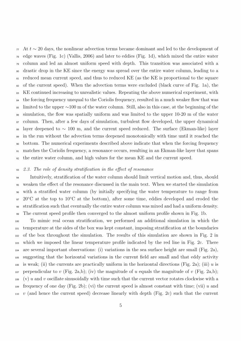
At t ∼ 20 days, the nonlinear advection terms became dominant and led to the development of77
edge waves (Fig. 1c) (Vallis, 2006) and later to eddies (Fig. 1d), which mixed the entire water78
column and led an almost uniform speed with depth. This transition was associated with a79
drastic drop in the KE since the energy was spread over the entire water column, leading to a80
reduced mean current speed, and thus to reduced KE (as the KE is proportional to the square81
of the current speed). When the advection terms were excluded (black curve of Fig. 1a), the82
KE continued increasing to unrealistic values. Repeating the above numerical experiment, with83
the forcing frequency unequal to the Coriolis frequency, resulted in a much weaker flow that was84
limited to the upper ∼100 m of the water column. Still, also in this case, at the beginning of the85
simulation, the flow was spatially uniform and was limited to the upper 10-20 m of the water86
column. Then, after a few days of simulation, turbulent flow developed, the upper dynamical87
layer deepened to ∼ 100 m, and the current speed reduced. The surface (Ekman-like) layer88
in the run without the advection terms deepened monotonically with time until it reached the89
bottom. The numerical experiments described above indicate that when the forcing frequency90
matches the Coriolis frequency, a resonance occurs, resulting in an Ekman-like layer that spans91
the entire water column, and high values for the mean KE and the current speed.92
2.3. The role of density stratification in the effect of resonance93
Intuitively, stratification of the water column should limit vertical motion and, thus, should94
weaken the effect of the resonance discussed in the main text. When we started the simulation95
with a stratified water column (by initially specifying the water temperature to range from96
20◦C at the top to 10◦C at the bottom), after some time, eddies developed and eroded the97
stratification such that eventually the entire water column was mixed and had a uniform density.98
The current speed profile then converged to the almost uniform profile shown in Fig. 1b.99
To mimic real ocean stratification, we performed an additional simulation in which the100
temperature at the sides of the box was kept constant, imposing stratification at the boundaries101
of the box throughout the simulation. The results of this simulation are shown in Fig. 2 in102
which we imposed the linear temperature profile indicated by the red line in Fig. 2c. There103
are several important observations: (i) variations in the sea surface height are small (Fig. 2a),104
suggesting that the horizontal variations in the current field are small and that eddy activity105
is weak; (ii) the currents are practically uniform in the horizontal directions (Fig. 2a); (iii) u is106
perpendicular to v (Fig. 2a,b); (iv) the magnitude of u equals the magnitude of v (Fig. 2a,b);107
(v) u and v oscillate sinusoidally with time such that the current vector rotates clockwise with a108
frequency of one day (Fig. 2b); (vi) the current speed is almost constant with time; (vii) u and109
v (and hence the current speed) decrease linearly with depth (Fig. 2c) such that the current110
5

x (km)
y(k
m)
(a)
η(m
m)
0.2 0.4 0.6 0.8 1
0.2
0.4
0.6
0.8
1
−6
−5
−4
−3
−2
0 1 2 3 4 5−6
−4
−2
0
2
4
6
velocity
(m/s)
t (days)
(b)
uv
|q |
−1 0 1 2 3 4 5 6
−1
−0.8
−0.6
−0.4
−0.2
0
u, v (m/s)
z(k
m)
uv
10 12 14 16 18 20
−1
−0.8
−0.6
−0.4
−0.2
0
T (oC)
(c)
0 0.005 0.01 0.015 0.020
1
2
3
4
5
x 10−3
Tz (oC/m)
|q| z
(1/s)
(d)
MITgcmτ0
2ρ0ν
τ0
2ρ0ν(1 − e−
aHT0
Tz)
Figure 2: (a) Section of (1 × 1 km of the 10 × 10 km domain) sea surface height (color) and surface current(arrows) under stratification conditions. The white arrows indicate the current field after six hours of the blackarrows, indicating clockwise rotation of the current field with the Coriolis frequency. (b) u (blue), v (green) andcurrent speed (red) as a function of time. (c) u (blue open circle), v (blue full circle) as a function of depth undertemperature stratification conditions (red curve). (d) Gradient in current speed as a function of stratificationtemperature gradient for the MITgcm simulations (blue open circles) and for the exponential fit (red curve)similar to Eq. (1). The filled green circle indicates the theoretically predicted current speed, τ0/(2ρ0ν), undervery strong stratification (Tz → ∞). Parameter values: τ0 = 0.1 N m−2, ρ0=1028 kg m−3, ν = 0.01 m2 s−1,ω0 = f = 2π/86400 s−1, H = 1.2 km, T0 = 15 ◦C, and a = 5.25.
6

vector direction is constant with depth; and (viii) the slope of linear decrease of the current111
speed from (vii) converges to a constant value for sufficiently strong stratification (Fig. 2d).112
It is clear that for sufficiently strong imposed stratification, the developed flow will not be113
able to break the stratification as the Richardson number will be very large and the stratified114
shear flow will be stable (Cushman-Roisin, 1994). We thus expect the slope |q|z (where q = u+iv115
— see the next section for more details) to converge exponentially to a limiting value with the116
level of stratification Tz. The two limits of this dependence can be deduced from our analysis:117
when Tz → 0 also |q|z → 0 (Fig. 1), and when Tz → ∞, Eq. (15) holds and |q|z = τ02ρ0ν
(see118
below). Thus, if ρz = const, then119
|q|z =τ0
2ρ0ν
(1− e
aHρ0ρz), (1)
where a is a constant that quantifies the decay rate and can be estimated from the simulated120
currents. It is possible to obtain the interior ocean profile by integrating Eq. (1)121
|q(z)| = τ02ρ0ν
(z +H)− τ02ρ0ν
eaHρ0ρz (z +H − h0) , (2)
where h0 is an additional constant that can be estimated from the simulations.122
In the following we consider two cases–one of uniform density and one of very strongly123
stratified ocean. In reality neither of these cases is valid as in the more realistic case the124
stratification is finite and internal wave dynamics and geostrophic turbulence should be taken125
into account. The specific exponential fit shown in Fig. 2d [following Eqs. (1) and (2)] is valid126
for the specifications listed in Sec. 2.1 and is probably different under different specifications.127
3. Model and solution procedure128
After a sufficiently long time, the simulated currents are almost uniform in the horizontal129
directions, in both the barotropic (constant density) and the stratified water column cases;130
see 2.3. We thus assumed, in the following, that the current’s components (u, v) very weakly131
depend on the horizontal dimensions (x, y) such that it is possible to omit the advection terms132
and the horizontal viscosity terms from the governing equations. Then, one is left with the133
Ekman model (Ekman, 1905):134
ut − fv = νuzz, (3)
vt + fu = νvzz, (4)
7

where t and z are the time and depth coordinates, f is the (constant) Coriolis frequency, and ν is135
the eddy-parameterized vertical viscosity coefficient. u and v, can be regarded as the velocities136
around the interior geostrophic currents (if these do exist) and thus the omission of the pressure137
gradient terms in Eqs. (3), (4). It is possible to obtain a single equation qt + ifq = νqzz, using138
a complex velocity variable, q = u + iv; we then applied a (time) Fourier Transform (FT) to139
obtain an equation with respect to the depth variable z:140
qzz − i(f + ω)q/ν = 0, (5)
where ω is the frequency variable and the “hat” indicates the FT.141
To close the solution of Eq. (5), we applied no-slip boundary conditions at the bottom of142
the ocean, q(z = −H) = 0, and at the surface, we linked the wind stress τ = τx + iτy (τx, τy are143
the x, y components of the wind-stress vector) to the surface currents by qz(z = 0) = τ /(ρ0ν)144
(Gill, 1982), where ρ0 is the ocean water density. The solution is then145
q =τ(1− i)d
2ρ0ν
e(1+i)(z+H)/d − e−(1+i)(z+H)/d
e(1+i)H/d + e−(1+i)H/d, (6)
where d =√
2ν/|f + ω| is the “spectral” Ekman layer depth.146
The FT of the second moment of the currents is given by147
|q|2 =|τ |2d22ρ20ν
2
cosh[2(z+H)
d
]− cos
[2(z+H)
d
]
cosh[2Hd
]+ cos
[2Hd
] . (7)
The frequency spectrum of the KE per unit area is then148
Ek =1
2
0∫
−H
|q|2dz =|τ |2d38ρ20ν
2
sinh(2Hd
)− sin
(2Hd
)
cosh(2Hd
)+ cos
(2Hd
) . (8)
The depth of the Ekman layer, d, diverges when ω = −f , and the wind-induced currents may149
reach the bottom of the ocean, depending on the frequency spectrum of the wind stress, τ .150
To explicitly find the currents, one must know the wind stress and must either apply an151
inverse FT or use Parseval’s theorem, i.e.,152
〈|q|2〉 =1
2π
∞∫
−∞
|q|2dω. (9)
8

We considered two cases, shown below: (i) a purely periodic wind stress, and (ii) stochastic153
wind stress with temporally decaying correlations.154
4. Periodic wind stress155
For simplicity, we chose the wind stress to be periodic only in the x direction such that156
τ(t) = τx,0 cos(ω0t) where τx,0 is the wind-stress amplitude in the x directions and ω0 is the157
frequency; below, for convenience, we drop the subscript x. The FT of the wind stress is then158
a sum of two δ functions and hence159
q(t) =
√2τ0
4ρ0ν
∑
j=+,−
d(jω0)sinh
[(1+i)(z+H)d(jω0)
]
cosh[(1+i)Hd(jω0)
] ei(jω0t−π4 ). (10)
The second moment of the currents is then160
〈q2〉 =τ 20
8ρ20ν2
∑
j=+,−
[d(jω0)]2cosh
[2(z+H)d(jω0)
]− cos
[2(z+H)d(jω0)
]
cosh[
2Hd(jω0)
]+ cos
[2H
d(jω0)
] , (11)
and the KE is161
Ek =τ 20
32ρ20ν2
∑
j=+,−
[d(jω0)]3
sinh[
2Hd(jω0)
]− sin
[2H
d(jω0)
]
cosh[
2Hd(jω0)
]+ cos
[2H
d(jω0)
] . (12)
Generally speaking, the depth of the Ekman layer, d, is much smaller than the depth of the162
ocean, H. In this case, the currents decay exponentially with depth and Eqs. (10)-(12) become163
independent of the ocean depth H; the current vector exhibits a periodic clockwise rotation164
with frequency ω0.165
In the case of “resonance,” the wind-stress frequency equals the Coriolis frequency (ω0 =166
−f) and the depth of the Ekman layer, d(ω0) =√
2ν/|f + ω0|, becomes infinite and, hence,167
much larger than the depth of the ocean. Thus, d(−f) → ∞ and d(f) =√ν/f . Then, based168
on Eq. (10), when the ocean is deep enough (i.e., H � d(f)), q may be approximated as169
q(t) =τ0
2ρ0ν
[d(f)√
2e(1+i)z/d(f)+i(ft−π/4) + (z +H)e−ift
](13)
such that both surface and bottom boundary conditions are satisfied. The current vector may170
9

be further approximated as171
[u(t), v(t)] = (z +H)τ0[cos(ft),− sin(ft)]/(2ρ0ν). (14)
Consequently, the current’s second moment and KE are172
|q|2 =τ 20
4ρ20ν2(z +H)2 (15)
Ek =τ 20
24ρ20ν2H3. (16)
Hence, under resonance conditions: (i) the current’s magnitude depends on the depth of the173
ocean and decreases linearly with depth to the bottom of the ocean, (ii) the current vector174
rotates clockwise with the Coriolis frequency, with a fixed magnitude, and (iii) the KE increases175
like H3.176
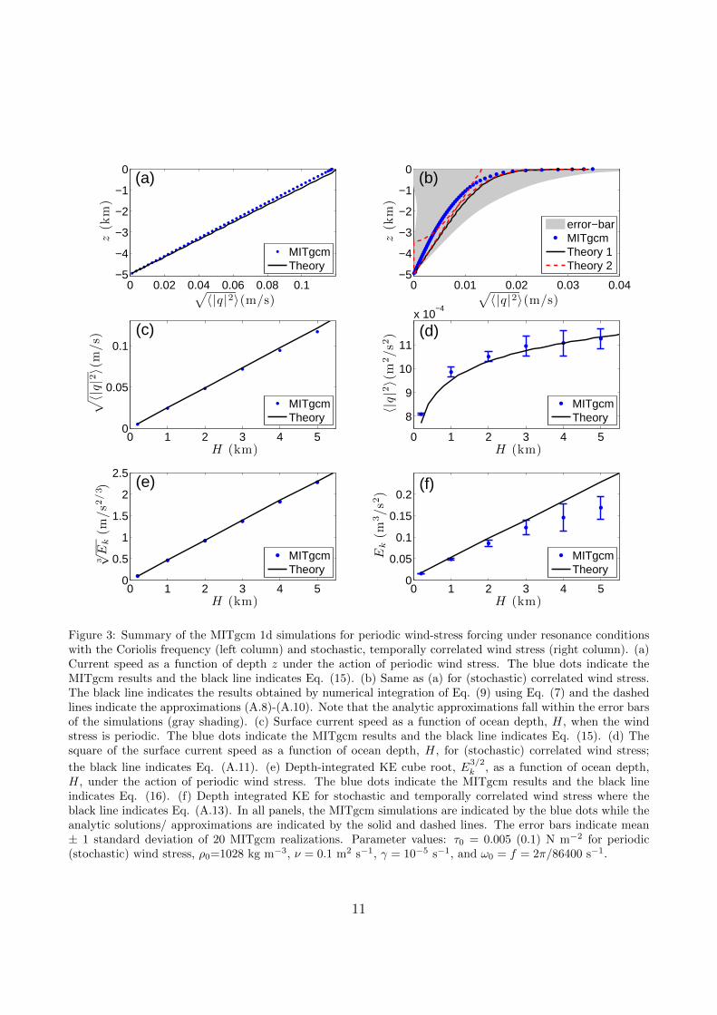
We validated the analytic solutions given above by comparing them with the MITgcm177
simulations. In these simulations, we focused on resonance conditions, excluding the spatial178
dependence. The results are shown in the left column of Fig. 3. The analytic solutions (black179
lines) are very close to the numerical ones (blue full circles), including (i) the clockwise rotation180
of the current vector with the Coriolis frequency (not shown), (ii) the linear decrease of the181
current speed with depth z (Fig. 3a), (iii) the linear increase of the surface current speed with182
the depth of the ocean, H (Fig. 3c), and (iv) the cubic dependence of the KE on the depth183
of the ocean, H (Fig. 3e). Under non-resonance conditions, the currents are limited to the184
surface Ekman layer and are independent of the depth of the ocean. It is important to note185
that when the current’s components u and v depend linearly on depth z, the viscosity terms186
in Eqs. (3),(4) vanish such that the equations take the form of the equations associated with187
the inertial oscillations that exhibit a clockwise rotation of the current vector with the Coriolis188
frequency.189
Resonance of the Coriolis force with other driving forces, such as diurnal winds or tides,190
is limited to a very narrow band of latitudes, questioning the overall effect of the resonance191
on real ocean circulation and energy. However, winds are stochastic in their nature such that192
one component of their frequency spectrum may resonate with the Coriolis force across the193
globe. This may lead to an enhancement of wind-induced currents over wide regions, possibly194
penetrating to the bottom of the ocean. We studied this hypothesis, as shown below.195
10
0 0.02 0.04 0.06 0.08 0.1−5
−4
−3
−2
−1
0
z(k
m)
√〈|q |2〉(m/s)
(a)
MITgcmTheory
−5
−4
−3
−2
−1
0
0 0.01 0.02 0.03 0.04
z(k
m)
√〈|q|2〉(m/s)
(b)
error−barMITgcmTheory 1Theory 2
0 1 2 3 4 50
0.05
0.1
H (km)
√〈|q|2〉(m/s)
(c)
MITgcmTheory
0 1 2 3 4 50
0.5
1
1.5
2
2.5
H (km)
3√E
k(m
/s2
/3 ) (e)
MITgcmTheory
0 1 2 3 4 5
8
9
10
11
x 10−4
H (km)
〈|q|2〉(m
2/s2) (d)
MITgcmTheory
0 1 2 3 4 50
0.05
0.1
0.15
0.2
H (km)
Ek(m
3/s2)
(f)
MITgcmTheory
Figure 3: Summary of the MITgcm 1d simulations for periodic wind-stress forcing under resonance conditionswith the Coriolis frequency (left column) and stochastic, temporally correlated wind stress (right column). (a)Current speed as a function of depth z under the action of periodic wind stress. The blue dots indicate theMITgcm results and the black line indicates Eq. (15). (b) Same as (a) for (stochastic) correlated wind stress.The black line indicates the results obtained by numerical integration of Eq. (9) using Eq. (7) and the dashedlines indicate the approximations (A.8)-(A.10). Note that the analytic approximations fall within the error barsof the simulations (gray shading). (c) Surface current speed as a function of ocean depth, H, when the windstress is periodic. The blue dots indicate the MITgcm results and the black line indicates Eq. (15). (d) Thesquare of the surface current speed as a function of ocean depth, H, for (stochastic) correlated wind stress;
the black line indicates Eq. (A.11). (e) Depth-integrated KE cube root, E3/2k , as a function of ocean depth,
H, under the action of periodic wind stress. The blue dots indicate the MITgcm results and the black lineindicates Eq. (16). (f) Depth integrated KE for stochastic and temporally correlated wind stress where theblack line indicates Eq. (A.13). In all panels, the MITgcm simulations are indicated by the blue dots while theanalytic solutions/ approximations are indicated by the solid and dashed lines. The error bars indicate mean± 1 standard deviation of 20 MITgcm realizations. Parameter values: τ0 = 0.005 (0.1) N m−2 for periodic(stochastic) wind stress, ρ0=1028 kg m−3, ν = 0.1 m2 s−1, γ = 10−5 s−1, and ω0 = f = 2π/86400 s−1.
11

5. Stochastic wind stress196
To study the effect of stochastic wind on ocean currents, we forced the model with a stochas-197
tic wind, whose temporal correlations decay exponentially,198
〈τ(t)τ(t+ t)〉 =τ 202e−γ|t| (17)
where τ0 is a parameter that quantifies the magnitude of the wind stress, and γ is a parameter199
that quantifies the decay rate of the temporal correlations (Bel and Ashkenazy, 2013; Ashkenazy200
et al., 2015). Similar to the above, for simplicity, we restricted the winds to be along the x201
direction. The FT of the wind stress (17) is202
|τ |2 =γτ 20
γ2 + ω2. (18)
We first used this wind stress to simulate currents using the MITgcm. The configuration was203
the same as the example presented above, i.e., a domain of 100 × 100 horizontal grid points204
with a resolution of 100 m and a 1.2-km-deep ocean, with doubly periodic boundary conditions.205
This configuration and forcing resulted in (spatially) almost uniform currents. We thus used the206
spatially independent Eqs. (3),(4) and the implicit solution (7) to gain greater understanding207
of the system’s dynamics. We developed, in Appendix A, analytic approximations for the208
dependence of the second moments of the current speed |q|2 on depth z, for the dependence209
of the surface current speed on ocean depth H, and for the dependence of the KE on ocean210
depth, Ek(H).211
We show that when the wind stress is stochastic with exponentially decaying temporal212
correlations, the current speed is not limited to the upper ocean but decreases linearly in the213
lower part of the ocean and vanishes only at the ocean floor; see Fig. 3b and Eq. (A.8). This is214
due to the “resonance” of the Coriolis force with the wind stress at the Coriolis frequency. At215
this frequency, the Ekman layer becomes infinite, leading to the penetration of wind-induced216
currents to the bottom of the ocean. The decrease is faster at the upper part of the ocean217
[Fig. 3b and Eqs. (A.9),(A.10)]. The MITgcm simulations exhibit a similar decrease with218
depth (full circles in Fig. 3b).219
The second moment of the surface current speed, |q|2 as a function ocean depth, H, is shown220
in Fig. 3d. The analytic approximation (A.11) indicates a logarithmic increase of |q|2 with H221
and is in good agreement with the MITgcm simulations (Fig. 3d). The analytic approximation222
of the KE, Eq. (A.15), points to a linear increase with the ocean depth, H. The agreement with223
12

the MITgcm simulations is satisfactory and better for shallower depths (Fig. 3f). In summary,224
under the action of temporally correlated stochastic wind stress, the currents are not confined225
in the upper ocean, as in the classical Ekman layer model, but extend to the bottom of the226
ocean.227
6. Implementation to the real ocean228
As the wind is stochastic and exhibits temporal correlations (Bel and Ashkenazy, 2013),229
the resonance of stochastic wind stress with the Coriolis force is relevant in extended regions230
of the globe. To get a rough idea of the effect of the resonance on the real ocean, we used the231
six-hourly winds of the NCEP-DOE reanalysis 2 (Kanamitsu et al., 2002). Yet, the analysis232
we present below does not meant to be realistic and is only aimed in highlighting the possible233
importance of Ekman resonance in the real ocean; this is unlike previous studies (e.g., Price234
et al., 1986) that presented realistic analysis on the effect of diurnal forcing on the ocean.235
Global-coverage (∼2.5◦) surface (10 m) winds of 36 years (1979-2014) were first transformed236
into wind stress based on Large and Yeager (2004):237
(τx, τy) = 10−3ρa(0.142U + 0.076U2 + 2.7)(ua, va), (19)
where ρa = 1.25 kg m−3 is the air density, U is the wind speed, and ua, va are zonal and238
meridional wind components. Then, we assumed, based on the data, that the auto-correlation239
function of the wind stress components follows:240
〈τx,y(t)τx,y(t+ t)〉 =1
2τx,y0 cos(ω0t) +
1
2τx,y1e
−γx,y |t|, (20)
where ω0 is the diurnal frequency. [We also estimated the KE based on the power spectrum of241
the wind stress and by directly numerically integrating Eq. (8) and obtained results that are242
very similar to the results described below. The advantage of using the present approach is243
the ability to estimate the contribution of the different components of the wind stress, namely244
the periodic and stochastic components of the wind stress (τx,y0 and τx,y1 respectively), and245
verify their relative importance.] Both τx,y0 and τx,y1 are calculated form the data: we first246
estimated τx,y0 from the FT of τx,y, then found τx,y1 from Eq. (20) at lag t = 0, then estimated247
the exponents γx,y from the auto-correlation function of the first four lags.248
The estimated exponents, γx,y, are shown in Fig. 4, and the two exhibit similar patterns.249
Generally speaking, the low latitudes (30◦S to 30◦N) are more correlated than the higher250
latitudes that are weakly correlated in regions of enhanced storm activity (e.g., the storm251
13

Figure 4: Temporal correlation exponents, (a) γx and (b) γy, in s−1, estimated based on the NCEP reanalysis2 surface (10 m) winds.
tracks and high mountains). The mean values of the exponents over the ocean are very similar252
to the mean value over the land and are 〈γx〉 = 10−5 s−1, 〈γy〉 = 1.2× 10⁻⁵ s−1.253
The different components of the wind stress are shown in Fig. 5. The correlated noise254
component, τ1 (Fig. 5a), is high in the regions of enhanced wind activity, such as the storm255
track and high mountains, and it roughly matches the regions of high correlation exponents256
γx,y shown in Fig. 4. τ1 is larger than the periodic wind component τ0 (Fig. 5b) by more257
than an order of magnitude. The periodic component is often large in regions of a large noise258
component, indicating that the periodicity is, in part, due to higher wind energy (power) in259
these regions. The mean wind-stress component, τm, is high only in the Southern Ocean and260
along the edge of Antarctica. The global mean values of τ1, τ0, τm over the ocean is 0.26,261
6.6 × 10⁻³, and 0.075 N m−2, respectively, and are very similar to the wind-stress values over262
14

Table 1: Summary of the different components of KE for NCEP-DOE and ERA-INTERIM reanalysis (in Joules).
NCEP-DOE ERA-INTERIMglobal mean deep ocean mean global mean deep ocean mean
Ek,1 7.27× 10¹⁷ 2.49× 10¹⁷ 2.66× 10¹⁷ 9.16× 10¹⁶
Ek,0 1.4× 10¹⁷ 6.04× 10¹⁶ 5.23× 10¹⁶ 2.51× 10¹⁶
Ek,m 6.44× 10¹⁵ 2.4× 10¹² 3.06× 10¹⁵ 1.31× 10¹¹
land.263
Given the wind-stress components, τx,y0,1,m, it is possible to calculate the KE that is asso-264
ciated with each of the components, based on the ocean depth at each grid point and based265
on Eqs. (7), (9). The KE of the entire water column is shown in Fig. 6. The KE associated266
with temporal correlation, Ek,1, is much larger than the other two components associated with267
the diurnal periodicity, Ek,0, and the mean wind stress, Ek,m. The global mean of the three268
components of the KE are listed in Table 1. [Analysis of the ERA-Interim (Berrisford et al.,269
2011) 6 hourly wind data yielded 2-3 times smaller KE; see Table 1.] While Ek,1 is significant270
in vast ocean regions, Ek,0 is very strong, as expected, around latitude 30◦. The estimated271
KE is obviously not realistic as it ignores all spatial dynamics and is about 1/5 of the realistic272
estimation of the global ocean KE ∼ 5.2× 10¹⁸J (vonStorch et al., 2012). The most important273
parameter is the viscosity coefficient, which was chosen to be 0.1 m2 s−1. We note that a smaller274
viscosity coefficient like 0.01 m2 s−1 (Cushman-Roisin, 1994) or even smaller (Gill, 1982) would275
yield much larger KE and the KE is inversely proportional of the viscosity coefficient; see Eq.276
A.15. It is reasonable that ν is much smaller at a depth where the eddy activity is weaker277
(similar to the effect of weak stratification on the diffusion coefficient, (Gargett, 1984)) such278
that the resultant currents will be stronger, leading to a larger KE.279
We have also calculated the KE of the deep ocean (deeper than 1 km) and found that280
a significant part is stored in the deep ocean. Fig. 7 depicts the ratio, r, between the deep281
ocean KE and the entire water column KE and, consistent with our predictions, the stochastic282
(Fig. 7a) and periodic (Fig. 7b) components of the wind stress account for tens of percentage283
points of the total KE. The deep ocean KE that resulted from the mean forcing (Fig. 7c) is,284
as expected, negligible; see Table 1. The ratio of global mean KE to the global mean deep285
ocean KE of the different components is r1 = 34%, r0 = 44% and rm = 0.04% indicating that286
indeed significant part of the KE is stored in the deep ocean; see Table 1. The ratio captures287
the pattern of the deep ridges as the KE depends on ocean depth H.288
The above calculations were based on the assumption that the ocean is strongly stratified.289
However, the deep ocean is only weakly stratified, such that one expects weaker currents and KE290
15

Figure 5: Wind-stress coefficient (in N m−2) of the (a) stochastic, τ1 =√τ2x,1 + τ2y,1, (b) periodic, τ0 =
√τ2x,0 + τ2y,0, and (c) mean, τm =
√〈τx〉2 + 〈τy〉2, components of the wind stress. Estimated based on the
NCEP reanalysis 2 surface (10 m) winds.
16

Figure 6: KE wind-stress coefficient (in N m−2) of the (a) stochastic, τ1, (b) periodic, τ0, and (c) mean, τm,components of the wind stress. Estimated based on the NCEP reanalysis 2 surface (10 m) winds.
17

Figure 7: Ratio between the KE of the deep ocean (deeper than 1 km) and the entire water column KE forthe (a) stochastic, (b) periodic, and (c) mean components of the wind stress. Estimated based on the NCEPreanalysis 2 surface (10 m) winds and the numerical integration of Eq. (8).
18

(see Fig. 2). The MITgcm simulations with an open boundary restoration of the temperature291
and salinity of the global and temporal mean of the Levitus atlas (Levitus, 1982) resulted in292
a linearly decreasing current speed in the few upper kms of the ocean and an almost uniform293
current speed in the abyssal ocean. However, the eddy viscosity coefficient may be smaller294
under such conditions due to the weaker eddy activity, probably leading to stronger currents295
and, hence, larger KE. Thus, the values given above only very roughly estimate the ocean’s296
KE.297
Following the above, our calculations indicate that the contribution of the stochastic wind298
stress is relevant in vast ocean regions and is much larger than the periodic wind stress compo-299
nent that is restricted to the 30◦ latitude. In addition, 34% of the energy due to the resonance300
of the Coriolis force with the stochastic part of the wind is absorbed in the deep ocean (deeper301
than 1 km). The contribution associated with the mean wind stress is much smaller than302
the contribution due to the stochastic and periodic parts of the wind stress, and is negligible303
in the deep ocean. While these estimations are based on realistic wind stress, they are very304
rough due to the simplistic assumptions of our approach, in particular due to the choice of the305
eddy-parameterized viscosity coefficient, ν, which depends on the eddy activity. In addition,306
we assumed that the eddy viscosity coefficient is constant both in time and space while, in fact,307
this is probably not the case. For example, the viscosity coefficient may drastically increase308
when a storm frequency matches the inertial frequency and the mixed layer deepens (Pollard309
et al., 1973). Moreover, dispersion, due to the variations in the Coriolis force (Anderson and310
Gill, 1979; D’Asaro, 1989) or other dispersion effects (Gill, 1984), also makes our estimation311
less accurate. In addition, it was shown that (a) stochastic winds in the Southern Ocean do312
not directly energize the deep ocean and that it is the work associated with the pressure field313
(Weijer and Gille, 2005) and (b) the wind energy input to the deep ocean may be drastically314
decreased due to dissipation processes and conversion to potential energy in the upper ocean315
(Furuichi et al., 2008; Zhai et al., 2009). Yet, our results indicate the penetration of wind316
energy to the deep ocean, even if the viscosity coefficient is large, and highlight the possible317
importance of the wind’s temporal variability on the transformation of wind KE to the deep318
ocean.319
7. Summary and conclusions320
In summary, we studied the role of the wind’s variability on deep ocean currents. We first321
showed, using the MITgcm, that when the wind is periodic with a frequency that matches322
the Coriolis frequency and when starting from rest, turbulent flow develops that eventually323
19
leads to the mixing of the entire water column and to a constant interior ocean current speed.324
Under stratification conditions imposed at the sides of the domain, the current speed decreases325
linearly with depth z and vanishes only at the bottom of the ocean. In all cases, the current326
field is almost laterally uniform, justifying the omission of the advection and lateral viscosity327
terms. We then provided an analytic solution for the currents under the action of periodic328
wind stress and found that the current speed decreases linearly with depth z and only vanishes329
at the ocean floor. The surface current speed depends linearly on the ocean depth, and the330
KE increases as a function of the cube of the ocean depth H. Under more realistic stochastic331
and temporally correlated wind stress, one of the wind’s frequencies resonates with the Coriolis332
force, causing the currents to reach the bottom of the ocean. We show, numerically and via333
analytic approximations, that the current speed in the deep ocean decreases linearly with depth334
z, that the second moment of the surface current increases logarithmically with the ocean depth335
H, and that the KE increases linearly as a function of ocean depth H. Thus, when considering336
the infinite depth Ekman layer model, an additional friction term must be included to avoid337
the singularity of the ocean currents (Kim et al., 2014; Ashkenazy et al., 2015).338
Under realistic global ocean bathymetry and realistic wind stress forcing, the contribution339
of the wind stress’s stochastic component is much larger than the contribution of the wind340
stress’s periodic component and the (temporal) mean wind stress, which is negligible. The341
stochastic component of the wind stress is significant in extended ocean areas, unlike the pe-342
riodic component which is significant only at 30◦ latitude, where the Coriolis force resonates343
with the diurnal winds. Moreover, around one-third of the KE is stored in ocean depths deeper344
than 1 km. While this is a very rough estimate due to the simplicity of the model, it indicates345
that the stochastic nature of the wind plays an important role in the energy budget of the deep346
ocean.347
8. Acknowledgment348
We thank Golan Bel, Georgy Burde, Hezi Gildor, Avi Gozolichiani, and Eli Tziperman for349
helpful discussions.350
Appendix A. Temporally correlated stochastic wind stress351
Given the FT of the of temporally correlated wind stress, Eq. (18), it is possible to find the352
FT of the second moment of the currents, using Eq. (7). The second moment of the currents353
is obtained by using the Parseval’s relation, Eq. (9). Eq. (7) is singular when ω = −f and the354
20

integral (9) around this point can be approximated as355
I2 =τ 20 (H + z)2
2πρ20ν2
ω2∫
ω1
γ
γ2 + ω2dω. (A.1)
Far from the point of singularity, Eq. (7) can be approximated as356
|q|2 ≈ |τ |2
ρ20ν
e2z/d
|f + ω| ≈|τ |2ρ20ν
1
|f + ω| . (A.2)
Then, when ω � −f , integral (9) can be approximated as357
I1 = − τ 202πρ20ν
ω1∫
ωl
γ
γ2 + ω2
1
f + ωdω, (A.3)
and when ω � −f , it can be approximated as358
I3 =τ 20
2πρ20ν
ωr∫
ω2
γ
γ2 + ω2
1
f + ωdω. (A.4)
The limits ω1,2 of I1,2,3 connect the different regions of the integral and are found based on the359
numerical results:360
ω1,2 = ∓ πνH2− f. (A.5)
The limits ωl,r are found such that the linear approximation of the exponent in Eq. (A.2) is361
zero,362
ωl,r = ∓ ν
2z2− f. (A.6)
Given the above limits, I2 is found to be363
I2 =τ 20 (H + z)2
2πρ20ν2
[tan−1
(πν
γH2− f
γ
)+ tan−1
(πν
γH2+f
γ
)]. (A.7)
I2 can be further approximated as364
I2 ≈τ 20 (H + z)2
ρ20ν
γ
f 2 + γ2. (A.8)
21
We find that I2 reproduces fairly well the second moment of the current speed close to the365
bottom.366
Close to the surface of the ocean, the second moment of the currents can be approximated367
by I1 + I3, which can be expressed, given the limits ωl,1,2,r, as follows:368
I1 =τ 20
4π(γ2 + f 2)ρ20ν[2f
(tan−1
(πν
γH2+f
γ
)− tan−1
(ν
2γz2+f
γ
))+
γ lnγ2H4 + (πν +H2f)2
4π2γ2z4 + (ν + 2fz2)2
](A.9)
I3 =τ 20
4π(γ2 + f 2)ρ20ν[2f
(tan−1
(ν
2γz2− f
γ
)− tan−1
(πν
γH2− f
γ
))+
γ lnγ2H4 + (πν −H2f)2
4π2γ2z4 + (ν − 2fz2)2
]. (A.10)
Thus, following Eq. (A.8), close to the bottom, the current speed decreases linearly with depth,369
z. A simple analysis of I1 + I3 of Eqs. (A.9),(A.10) indicates that close to the surface of the370
ocean, the decrease of current speed with depth z is approximately logarithmic.371
Based on I1 + I3 of Eqs. (A.9),(A.10), we approximate the second moment of the surface372
current (z = 0) as373
|q|2 ≈ τ 20π(γ2 + f 2)ρ20ν
[f tan−1
(f
γ
)+
γ ln
(√γ2 + f 2
ν
)+ 2γ lnH
]. (A.11)
Thus, |q|2 grows logarithmically with the ocean depth, H.374
It is possible to approximate the total KE in a way similar to the above treatment. Based375
on Eq. (8), the FT of the KE close to the singularity point (ω = −f) is approximated as376
Ek ≈|τ |2H3
6ρ20ν2, (A.12)
22
and given Eqs. (18), (9), the KE is then377
Ek ≈τ 20H
3
12πρ20ν2
ω2∫
ω1
γ
ω2 + γ2dω =
τ 20H3
12πρ20ν2
[tan−1
(3πν
2γH2− f
γ
)+ tan−1
(3πν
2γH2+f
γ
)], (A.13)
where the limits ω1,2 are378
ω1,2 = ∓ 3πν
2H2− f. (A.14)
As the depth of the ocean is usually much larger than the depth of the Ekman layer (i.e.,379
H2 � 3π4
2νf
), the KE can be further simplified,380
Ek ≈γτ 20
4ρ20ν(γ2 + f 2)H. (A.15)
Thus, when the wind stress is stochastic with exponentially decaying correlations, the KE381
increases linearly with the depth of the ocean H.382
Alford, M.H., MacKinnon, J.A., Simmons, H.L., Nash, J.D., 2016. Near-inertial internal gravity383
waves in the ocean. Annual review of marine science 8, 95–123.384
Anderson, D.L.T., Gill, A.E., 1979. Beta dispersion of inertial waves. J. Geophys. Res. 84,385
1836–1842.386
Ashkenazy, Y., Gildor, H., Bel, G., 2015. The effect of stochastic wind on the infinite depth387
Ekman layer model. Europhysics Lett. accepted.388
Bel, G., Ashkenazy, Y., 2013. The relationship between the statistics of open ocean currents389
and the temporal correlations of the wind. New J. Phys. 15, 053024.390
Berrisford, P., Dee, D., Poli, P., Brugge, R., Fielding, K., Fuentes, M., Kallberg, P., Kobayashi,391
S., Uppala, S., Simmons, A., 2011. The era-interim archive version 2.0. Shinfield Park,392
Reading.393
Chang, S.W., Anthes, R.A., 1978. Numerical simulations of the ocean’s nonlinear, baroclinic394
response to translating hurricanes. J. Phys. Oceanogr. 8, 468–480.395
Crawford, G.B., Large, W.G., 1996. A numerical investigation of resonant inertial response of396
the ocean to wind forcing. J. Phys. Oceanogr. 26, 873–891.397
23

Cushman-Roisin, B., 1994. Introduction to geophysical fluid dynamics. Prentice Hall. 1st398
edition.399
Danioux, E., Klein, P., 2008. A resonance mechanism leading to wind-forced motions with a 2400
f frequency. Journal of Physical Oceanography 38, 2322–2329.401
Danioux, E., Klein, P., Riviere, P., 2008. Propagation of wind energy into the deep ocean402
through a fully turbulent mesoscale eddy field. Journal of Physical Oceanography 38, 2224–403
2241.404
D’Asaro, E.A., 1989. The decay of wind-forced mixed layer inertial oscillations due to the β405
effect. Journal of Geophysical Research: Oceans 94, 2045–2056.406
Defant, A., 1961. Physical oceanography; volume 2 .407
Dewar, W.K., Bingham, R.J., Iverson, R., Nowacek, D.P., St Laurent, L.C., Wiebe, P.H., 2006.408
Does the marine biosphere mix the ocean? Journal of Marine Research 64, 541–561.409
Ekman, V.W., 1905. On the influence of the earth’s rotation in ocean-currents. Arch. Math.410
Astron. Phys. 2, 1–52.411
Furuichi, N., Hibiya, T., Niwa, Y., 2008. Model-predicted distribution of wind-induced internal412
wave energy in the world’s oceans. Journal of Geophysical Research: Oceans (1978–2012)413
113.414
Gargett, A., 1984. Vertical eddy diffusivity in the ocean interior. J. Mar. Res. 42, 359–393.415
Gill, A., 1984. On the behavior of internal waves in the wakes of storms. Journal of Physical416
Oceanography 14, 1129–1151.417
Gill, A.E., 1982. Atmosphere–ocean dynamics. Academic Press, London.418
Gonella, J., 1971. A local study of inertial oscillations in the up- per layers of the ocean. Deep419
Sea Res. 18, 775–788.420
Greatbatch, R.J., 1983. On the response of the ocean to a moving storm: The nonlinear421
dynamics. J. Phys. Oceanogr. 13, 357–367.422
Greatbatch, R.J., 1984. On the response of the ocean to a moving storm: Parameters and423
scales. J. Phys. Oceanogr. 14, 59–78.424
24

Huang, R.X., 1999. Mixing and energetics of the oceanic thermohaline circulation. J. Phys.425
Oceanogr. 29, 727–746.426
Kanamitsu, M., Ebisuzaki, W., Woollen, J., Yang, S.K., Hnilo, J., Fiorino, M., Potter, G., 2002.427
NCEP-DOE AMIP-II reanalysis (r-2). Bulletin of the American Meteorological Society 83,428
1631–1643.429
Kim, S.Y., Kosro, P.M., Kurapov, A.L., 2014. Evaluation of directly wind-coherent near-inertial430
surface currents off Oregon using a statistical parameterization and analytical and numerical431
models. J. Geophys. Res. 119, 6631–6654.432
Large, W.G., Yeager, S.G., 2004. Diurnal to decadal global forcing for ocean and sea-ice models:433
the data sets and flux climatologies. Citeseer.434
Lee, D.K., Niiler, P.P., 1998. The inertial chimney: The near-inertial energy drainage from the435
ocean surface to the deep ocean. J. Geophys. Res. 103, 7579–7591.436
Levitus, S.E., 1982. Climatological atlas of the world ocean. NOAA Professional Paper 13, US437
Government Printing Office, Washington DC.438
McWilliams, J.C., Huckle, E., 2005. Ekman layer rectification. J. Phys. Oceanogr. 36, 1646–439
1659.440
Mickett, J.B., Serra, Y.L., Cronin, M.F., Alford, M.H., 2010. Resonant forcing of mixed layer441
inertial motions by atmospheric easterly waves in the northeast tropical Pacific. J. Phys.442
Oceanogr. 40, 401–416.443
MITgcm-group, 2010. MITgcm User Manual. Online doc-444
umentation. MIT/EAPS. Cambridge, MA 02139, USA.445
http://mitgcm.org/public/r2 manual/latest/online documents/manual.html.446
Munk, W., 1966. Abyssal recipes. Deep Sea Res. 13, 707–730.447
Munk, W., Wunsch, C., 1998. Abyssal recipes ii: energetics of tidal and wind mixing. Deep448
Sea Res. 45, 1977–2010.449
Pollard, R.T., Rhines, P.B., Thompson, R.O.R.Y., 1973. The deepening of the wind-mixed450
layer. Geophys. Fluid Dyn. 3, 381–404.451
Price, J.F., 1981. Upper ocean response to a hurricane. J. Phys. Oceanogr. 11, 153–175.452
25
Price, J.F., 1983. Internal wave wake of a moving storm. part i. scales, energy budget and453
observations. J. Phys. Oceanogr. 13, 949–965.454
Price, J.F., Weller, R.A., Pinkel, R., 1986. Diurnal Cycling: Observations and models of the455
upper ocean response to diurnal heating, cooling, and wind mixing. J. Geophys. Res. 91,456
8411–8427.457
Rudnick, D.L., 2003. Observations of momentum transfer in the upper ocean: Did Ekman get458
it right?, in: Muller, P., Henderson, D. (Eds.), Near-Boundary Processes and Their Parame-459
terization, Proceedings of the 13th ’Aha Huliko’a Hawaiian Winter Workshop, University of460
Hawaii. pp. 163–170.461
Rudnick, D.L., Weller, R., A., 1993. Observations of superinertial and near-inertial wind-driven462
flow. J. Phys. Oceanogr. 23, 2359–2351.463
Sandstrom, J.W., 1908. Dynamicsche versuche mit meerwasser. Annalen der Hydrographie464
under Martimen Meteorologie 36, 6–23.465
Stockwell, R.G., Large, W.G., Milliff, R.F., 2004. Resonant inertial oscillations in moored buoy466
ocean surface winds. Tellus A 56, 536–547.467
Vallis, G.K., 2006. Atmospheric and Oceanic Fluid Dynamics. Cambridge University Press,468
Cambridge, U.K.469
vonStorch, J.S., Eden, C., Fast, I., Haak, H., Hernandez-Deckers, D., Maier-Reimer, E.,470
Marotzke, J., Stammer, D., 2012. An estimate of the lorenz energy cycle for the world471
ocean based on the storm/ncep simulation. J. Phys. Oceanogr. 42, 2185–2205.472
Weijer, W., Gille, S.T., 2005. Energetics of wind-driven barotropic variability in the southern473
ocean. Journal of Marine Research 63, 1101–1125.474
Whitt, D.B., Thomas, L.N., 2015. Resonant generation and energetics of wind-forced near-475
inertial motions in a geostrophic flow. J. Phys. Oceanogr. 45, 181–208.476
Wunsch, C., Ferrari, R., 2004. Vertical mixing, energy and thegeneral circulation of the oceans.477
Ann. Rev. Fluid Mech. 36, 281–314.478
Zhai, X., 2015. Latitudinal dependence of wind-induced near-inertial energy. J. Phys. Oceanogr.479
45, 3025–3032.480
26

Zhai, X., Greatbatch, R.J., Eden, C., 2007. Spreading of near-inertial energy in a 1/12 model481
of the north atlantic ocean. Geophysical research letters 34.482
Zhai, X., Greatbatch, R.J., Eden, C., Hibiya, T., 2009. On the loss of wind-induced near-483
inertial energy to turbulent mixing in the upper ocean. Journal of Physical Oceanography484
39, 3040–3045.485
Zhai, X., Greatbatch, R.J., Zhao, J., 2005. Enhanced vertical propagation of storm-induced486
near-inertial energy in an eddying ocean channel model. Geophys. Res. Lett. 32.487
27