Energy Policy (2004) 32:5, 635-645.

Managing electricity procurement cost and risk by a local distribution company

Chi-Keung Woo*a, Rouslan I. Karimova, Ira Horowitzb

a Energy and Environmental Economics, Inc., 353 Sacramento Street, Suite 1700

San Francisco CA 94111

b Warrington College of Business, University of Florida, Gainesville FL 32611-7169

Abstract

A local electricity distribution company (LDC) can satisfy some of its future

electricity requirements through self-generation and volatile spot markets, and the

remainder through fixed-price forward contracts that will reduce its exposure to the

inherent risk of spot-price volatility. A theoretical framework is developed for

determining the forward-contract purchase that minimizes the LDC’s expected

procurement cost, subject to a cost-exposure constraint. The answers to the questions of

“What to buy?” and “How to buy?” are illustrated using an example of a hypothetical

LDC that is based on a municipal utility in Florida. It is shown that the LDC’s

procurement decision is consistent with least-cost procurement subject to a cost-exposure

constraint, and that an internet-based multi-round auction can produce competitive price

quotes for its desired forward purchase.

Keywords: Electricity procurement; Cost risk management; Electricity market reform

__________

* Corresponding author. Phone: 415-391-5100, Fax: 415-391-6500.

Email address: ck@ethree.com (C.K. Woo)

1

1. Introduction

Electricity market reform and deregulation have created wholesale spot markets

that are characterized by high price volatility (Woo, 2001; Borenstein, 2002; Wilson,

2002). In some instances that volatility can be attributed to the fact that electricity cannot

be economically stored and must be generated instantaneously to meet real-time demand.

Hence, a relatively small supply reduction, say due to forced plant outages, can cause

sharp spot-price spikes that are traced out along what tend to be relatively price-inelastic

spot-market demand curves. Conversely, when market supply approaches full generation

capacity, relatively small demand increases, say due to rising summer temperatures or

falling winter temperatures, can result in substantial price increases that are traced out

along the full-capacity inelastic supply curve.

Local distribution companies (LDCs) have the mandate to supply electricity, upon

demand, to the customers with whom they have contracted. An LDC has three basic

options for acquiring that electricity: (1) generation through its own plant facility; (2)

spot-market purchases; and (3) fixed-price forward contracts. The last option is brought

into play, and the LDC satisfies some of its anticipated future requirements through

forward contracts, in order to better manage the electricity procurement-cost risk that

stems from spot-price volatility. By entering into a forward contract, the LDC may be

able to avoid the potentially disastrous financial consequences of over-reliance on the

spot market, which were so dramatically evidenced by the April 2001 bankruptcy of

Pacific Gas and Electric Company (PG&E), one of the largest utilities in the United

States.

2

The California electricity crisis of 2000-2001 led to Governor Davis signing

Assembly Bill 57 on September 25, 2002, which requires each of the three large investor-

owned utilities, PG&E, Southern California Edison (SCE), and San Diego Gas and

Electric (SDGE), to file a procurement plan to achieve the goal of stable, just and

reasonable rates. Each plan must contain the filing utility’s risk-management policy and

strategy, the cost risk of the utility’s resource portfolio, the quantity and type of hedging

products to be procured (e.g., forward contracts and options), and the competitive process

(e.g., bilateral negotiation, brokerage service, or auction) for procuring such products.

The idea of using forward contracts to manage procurement-cost risk is intuitively

appealing. Nevertheless, its implementation necessitates a decision as to the amount of

forward electricity the LDC should purchase. The decision can be based on subjective

managerial judgments, on simple rules of thumb (e.g., not less than 95% of the LDC’s

forecast total electricity requirement (CPUC, 2002, p. 32)), or, as proposed in this paper,

on the solution to a risk-constrained least-cost procurement problem. After deciding on

the least-cost forward purchase, the LDC then makes the purchase via a competitive

procurement process.

This paper defines the LDC’s procurement problem, which is succinctly described

by two related questions: “What to buy?” and “How to buy?” We show that the answer

to “What to buy?” solves a risk-constrained expected-cost minimization problem. The

answer provides the optimal forward-contract purchase, given management’s perception

of the LDC’s customers’ risk tolerance, its projection of spot prices and their volatility in

a future delivery period, and the range of likely forward-contract price quotes from

prospective sellers.

3

Knowing what to buy, however, does not guarantee least-cost implementation,

because the forward-contract price quoted by a prospective seller may not be the “best

deal” that the LDC could have obtained. To see this, consider the standardized forward

contracts for next-month delivery that are actively traded at major electricity hubs in the

United States (e.g., Mid-Columbia in Washington, California-Oregon-Border in Oregon,

and Palo Verde in Arizona). These standardized contracts apply to a multiple of a 50-

megawatt (MW) energy block size for (6x16) delivery at 100% rate during 06:00-22:00,

Monday through Saturday. If its desired purchase is a standardized forward contract, the

LDC can simply buy from the actively traded forward market with many competing

sellers.

The forward contract of the LDC’s interest, however, often deviates from a

standardized contract. Common deviations include: (a) a delivery point different from a

major hub; (b) a contract period longer than the next month; (c) daily delivery pattern

different from the (6x16) specification; and (d) an MW size that is not a multiple of 50

MW. Trading for non-standardized contracts is either non-existent or very thin. As a

result, the LDC may not easily receive a competitive price quote for non-standardized

contracts without using an auction.1 This paper answers “How to buy?” by describing an

internet-based multi-round auction.

The answers for “What to buy?” and “How to buy?” are illustrated through an

example of a hypothetical LDC that is based on a small utility located in Florida. They

show the LDC’s procurement decision to be consistent with least-cost procurement

subject to a cost-exposure constraint, and that an internet-based multi-round auction can

produce competitive price quotes for its desired forward purchase.

4

The paper proceeds as follows. Section 2 characterizes the constrained least-cost

electricity procurement that answers “What to buy?” Section 3 implements the answer for

our hypothetical LDC. Section 4 describes the internet-based auction that answers “How

to buy?” Section 5 concludes.

2. Constrained Least-Cost Electricity Procurement

Consider an LDC that is legally obligated to provide electricity to its customers

during some future period t1. For simplicity, we assume that the LDC has neither existing

power-purchase contracts nor generation capacity. Thus the LDC relies on either the spot

market in period t1 or a forward contract entered into in period t0 to acquire the electricity

that it resells to those customers. Incorporating existing contract costs or fuel costs

associated with generation adds computational complexity without substantially

improving our understanding of the procurement problem.

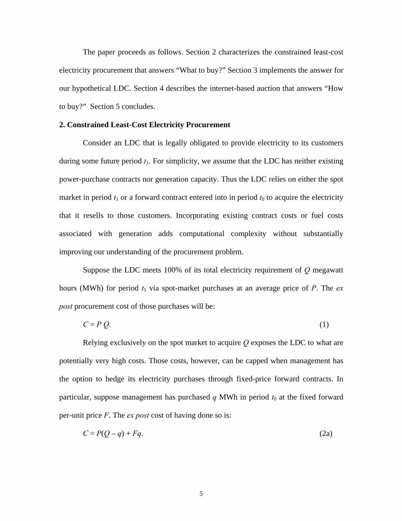
Suppose the LDC meets 100% of its total electricity requirement of Q megawatt

hours (MWh) for period t1 via spot-market purchases at an average price of P. The ex

post procurement cost of those purchases will be:

C = P Q. (1)

Relying exclusively on the spot market to acquire Q exposes the LDC to what are

potentially very high costs. Those costs, however, can be capped when management has

the option to hedge its electricity purchases through fixed-price forward contracts. In

particular, suppose management has purchased q MWh in period t0 at the fixed forward

per-unit price F. The ex post cost of having done so is:

C = P(Q – q) + Fq. (2a)

5

Equation (2a) shows that C converges to FQ as q approaches Q, and the forward

contract approaches meeting 100% of the LDC’s requirement. But while forward

contracting can reduce the cost effects of unanticipated spot-price changes, it cannot

eliminate the cost variations that are due to unanticipated changes in the consumer’s

demand for electricity, which the LDC is obligated to satisfy. That is, prior to its entering

into any forward contract, LDC management is forced to recognize that both P and Q are

random variables. Suppose for the moment that the expected values (variances) of those

random variables are known to be μP (σP2) and μQ (σQ

2), respectively, with a covariance

of σP,Q = ρσPσQ, where ρ is the correlation between P and Q. Casual observation leads

us to hypothesize ρ > 0. That is, spot-market demand changes tend to be more

responsible for spot-market price changes than supply changes. As we shall subsequently

demonstrate, the hypothesis is supported by the sample data that underlie our empirical

analysis.

At the time that it is considering its forward-contracting options, then, as far as

LDC management is concerned, the procurement cost C is also and necessarily a random

variable. When Q ≥ q, the LDC will purchase (Q – q) on the spot market at the price of P.

Suppose, however, that Q < q. In this event, as the owner of excess electricity, the LDC

enters the spot market as a seller, rather than as a buyer, and the P(Q – q) < 0 term in

equation (2a) reduces the procurement cost.

Rewrite equation (2a) as

C = PQ + (F – P)q. (2b)

Following Mood et al. (1974, p. 178), let E[PQ] = μPQ = μPμQ + ρσPσQ. The expected

procurement cost, μ, is then readily determined to be:

6

μ = μPQ + (F – μP) q. (3)

Since the forward-contract seller bears the spot-price risk, F commonly includes a

positive risk premium, so that (F – μP) > 0. Competition among sellers, however, serves

to drive F toward μP. Nonetheless, it is unlikely that F will be consistently below μP,

because from a seller’s perspective, the forward sale will on average be unprofitable

relative to the default alternative of a spot-market sale. Hence, we would expect dμ/dq =

(F - μP) > 0; or, μ increases with increases in q. To be sure, it is possible that a seller may

occasionally underestimate μP and make a forward-price offer below μP, in which case

dμ/dq < 0 and μ declines with increases in q.

For the purpose of risk management, the variance of C, ν = σ2, as a proxy

measure of risk, can be computed as follows (Mood et al., 1974, p. 179):

σ2 = σPQ2 + σP

2q2 - 2ρPQ,PσPQσPq. (4)

Here, σPQ2 denotes the variance of PQ and ρPQ,P denotes the correlation between PQ and

P.2 We expect ρPQ,P > 0 because P and Q are positively correlated.

The effect of the size of the forward contract on the procurement-cost variance is

seen through dν/dq = 2σP(σPq - ρPQ,PσPQ), which is negative (positive) when q is less

(greater) than ρPQ,PσPQ/σP. Moreover, σ2 is strictly convex in q because d2ν/dq2 = 2σP2 >

0. Thus, starting from an unhedged position of q = 0, a small forward purchase by the

LDC would reduce the cost variance. Additional forward purchases would minimize the

cost variance at q = ρPQ,PσPQ/σP. Forward purchases beyond this level, however, would

raise the cost variance.

Management’s problem can be formulated in the most straightforward fashion by

first making the convenient assumption that C is normally distributed. The validity of this

7

assumption in any specific application is necessarily subject to empirical verification. The

normality assumption is made here solely for expository purposes. If the normality

hypothesis is rejected, other familiar distributions (e.g., the t, the F, the chi-square, the

Gamma-2, etc.) can be put to the same test. Only the value of zα (assigned below) will be

affected. Indeed, in any actual application the distribution of C and the zα in question can

always be determined directly from the distributions of P and Q upon which management

will rely when making its contracting decision.

Suppose that management sets an upper-limit threshold of T on its procurement

cost C, such that the probability of C exceeding T is α. Denoting by zα the standard

normal variate so that, for example, at α = 0.05, zα = 1.645:

T = μ + zασ. (5)

Thus T is the cost exposure that an LDC would face under normal circumstances with a

probability of (1 – α). This definition of cost exposure is analogous to the value-at-risk

commonly used in financial risk management (Jorion, 1997).

How much forward electricity the LDC should buy depends on the risk tolerance

of the LDC’s customers, since the LDC only acts as a purchasing agent on their behalf.

Absent precise knowledge of customer risk preferences, however, management can use a

cost-exposure constraint to represent their risk tolerance:3

T < θμ. (6)

The multiplier θ reflects management’s perception of its customers’ tolerance for risk. If

management perceives that the LDC’s customers can tolerate a high cost exposure

relative to the expected-cost level, it would select a θ value substantially above 1. If,

8

however, management perceives low customer risk tolerance, it would select a θ value

close to 1 to reflect customer preference for a relatively small σ for a given value of zα.

Management’s problem is to choose q to minimize the expected procurement cost

described by equation (3), subject to the cost-exposure constraint given by equation (6),

as shown in Appendix A. Such an approach, however, may be seen as rather complicated

and abstruse by the LDC’s management or regulator. Moreover, the LDC’s procurement

report should contain data on cost expectation and exposure. Alternatively, management

can address the problem using a simple spreadsheet format that employs the following

heuristic procedure:

1. Set q at wμQ for delivery period t1, where 0 ≤ w ≤ 1 is a fraction of the

expected MWh requirement. In our illustration, we consider values of 0.0,

0.25, 0.50, 0.75, and 1.0.

2. Assume a forward price to compute the cost expectation and exposure for

each q value from Step 1. The range of assumed forward prices should reflect

μP and σP2.

3. Tabulate the results from Step 2.

3. Empirical Answer for “What to Buy?”

Our answer is based on the data collected for a municipal utility (MU) owned by

the residents of a city in Florida. (We cannot disclose the MU’s identity for contractual

reasons.) Interconnected to Florida Power and Light (FPL) and Florida Power Corp.

(FPC), the MU has limited generation and must procure electricity to meet its obligation

to serve its retail customers. With an annual peak of approximately 90 MW, the MU had

historically been buying most of its electricity requirement from FPL and FPC and the

9

remainder from the spot market. In August 2002, the MU decided to buy an energy block

at fixed price for daily delivery in October 2002 to reduce its exposure to the spot market

price volatility. The energy block is 20 MW for the peak hours of 12:00-20:00 and 15

MW for the shoulder hours of 07:00–12:00 and 20:00-23:00. Hence, the MU’s intended

purchase for October 2002 delivery is a fixed quantity of (20 MW x 8 hours per day + 15

MW x 8 hours per day) x 31 days = 8,680 megawatt-hours (MWh). Finally, the MU

decided that the entire forward purchase should be at a fixed price to be determined in an

auction to be held in September 2002.

We could have evaluated the MU’s forward purchase decision based on the fixed

quantity of 8,680 MWh. Such an evaluation, however, would not consider quantity

uncertainty, an important dimension of a typical procurement problem. Hence, for the

purpose of illustration, our example is a hypothetical LDC characterized by the following

assumptions:

• Its MWh requirement is the MU’s net MWh purchase (= total purchase less

sale) from the spot market.

• It faces the same spot purchase prices as the MU.

• Like the MU, it decides to use forward purchase to meet 100% of the assumed

requirement.

• Like the MU, it plans to use a procurement auction to find the “best” forward

price offer.

To evaluate this hypothetical LDC’s procurement decision, we first estimate the

components of μ and σ2, which, for our LDC, we denote u and s2, respectively. The

estimation entails the following steps:

10

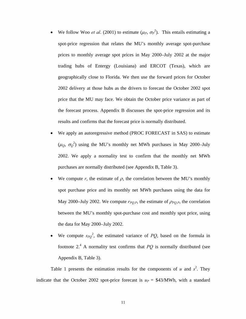
• We follow Woo et al. (2001) to estimate (μP, σP2). This entails estimating a

spot-price regression that relates the MU’s monthly average spot-purchase

prices to monthly average spot prices in May 2000–July 2002 at the major

trading hubs of Entergy (Louisiana) and ERCOT (Texas), which are

geographically close to Florida. We then use the forward prices for October

2002 delivery at those hubs as the drivers to forecast the October 2002 spot

price that the MU may face. We obtain the October price variance as part of

the forecast process. Appendix B discusses the spot-price regression and its

results and confirms that the forecast price is normally distributed.

• We apply an autoregressive method (PROC FORECAST in SAS) to estimate

(μQ, σQ2) using the MU’s monthly net MWh purchases in May 2000–July

2002. We apply a normality test to confirm that the monthly net MWh

purchases are normally distributed (see Appendix B, Table 3).

• We compute r, the estimate of ρ, the correlation between the MU’s monthly

spot purchase price and its monthly net MWh purchases using the data for

May 2000–July 2002. We compute rPQ,P, the estimate of ρPQ,P, the correlation

between the MU’s monthly spot-purchase cost and monthly spot price, using

the data for May 2000–July 2002.

• We compute sPQ2, the estimated variance of PQ, based on the formula in

footnote 2.4 A normality test confirms that PQ is normally distributed (see

Appendix B, Table 3).

Table 1 presents the estimation results for the components of u and s2. They

indicate that the October 2002 spot-price forecast is uP = $43/MWh, with a standard

11

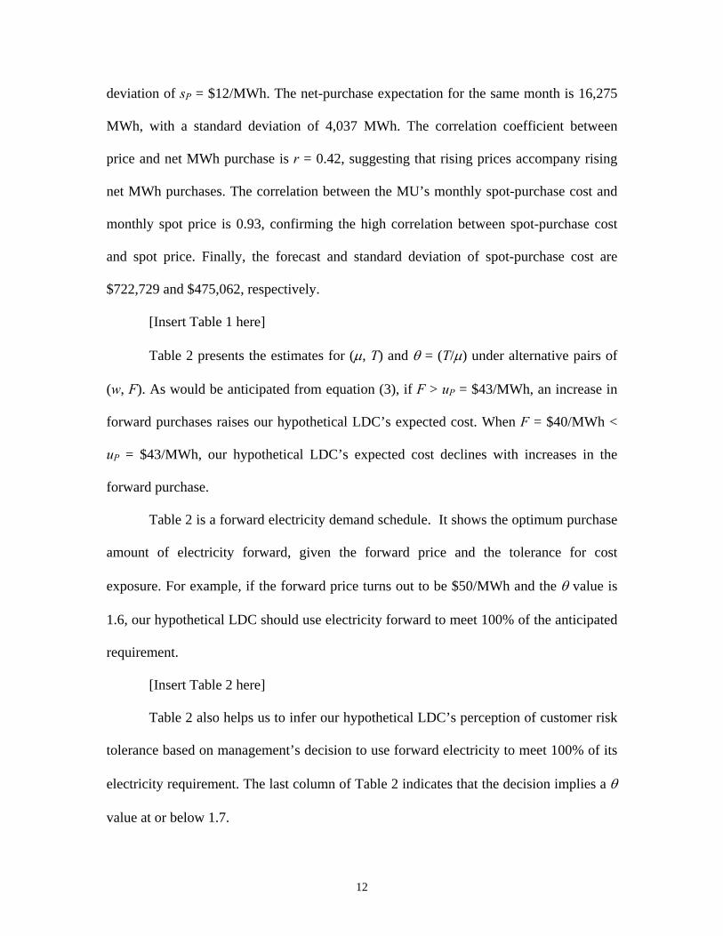
deviation of sP = $12/MWh. The net-purchase expectation for the same month is 16,275

MWh, with a standard deviation of 4,037 MWh. The correlation coefficient between

price and net MWh purchase is r = 0.42, suggesting that rising prices accompany rising

net MWh purchases. The correlation between the MU’s monthly spot-purchase cost and

monthly spot price is 0.93, confirming the high correlation between spot-purchase cost

and spot price. Finally, the forecast and standard deviation of spot-purchase cost are

$722,729 and $475,062, respectively.

[Insert Table 1 here]

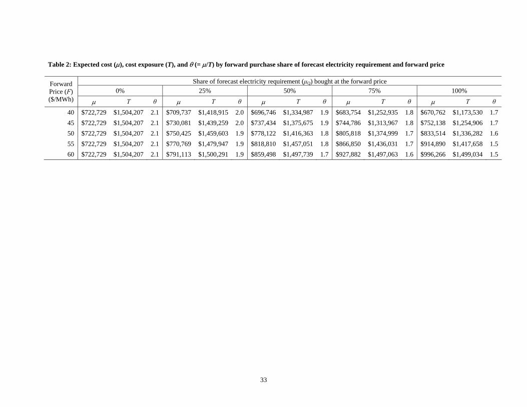
Table 2 presents the estimates for (μ, T) and θ = (T/μ) under alternative pairs of

(w, F). As would be anticipated from equation (3), if F > uP = $43/MWh, an increase in

forward purchases raises our hypothetical LDC’s expected cost. When F = $40/MWh <

uP = $43/MWh, our hypothetical LDC’s expected cost declines with increases in the

forward purchase.

Table 2 is a forward electricity demand schedule. It shows the optimum purchase

amount of electricity forward, given the forward price and the tolerance for cost

exposure. For example, if the forward price turns out to be $50/MWh and the θ value is

1.6, our hypothetical LDC should use electricity forward to meet 100% of the anticipated

requirement.

[Insert Table 2 here]

Table 2 also helps us to infer our hypothetical LDC’s perception of customer risk

tolerance based on management’s decision to use forward electricity to meet 100% of its

electricity requirement. The last column of Table 2 indicates that the decision implies a θ

value at or below 1.7.

12

4. Empirical Answer for “How to Buy?”

While our hypothetical LDC can use Table 2 to guide its forward purchase, it

cannot make the final decision without a binding forward-price quote. We assume that

like the MU, this LDC would hold an auction to obtain the quote. This section describes

the MU auction that answers “How to buy?”

4.1 The MU’s Extant Procurement Process

The MU held an internet-based procurement auction in September 2002, even

though it could have used its extant process to procure its desired forward contract. The

MU’s extant process is a request for offers (RFO) that solicits sealed offers from

suppliers, followed by final negotiation. Commonly used by LDCs for buying energy and

capacity, this kind of RFO process is equivalent to a single-round sealed-offer auction.

A single-round sealed-offer auction, however, may have several shortcomings

(Cameron et al., 1997). First, it may not inform a buyer like the MU of the “best deal”

available from the auction participants. While negotiation improves the final offer, its

outcome may still not be the result of the fierce head-to-head competition exemplified by

an open-offer auction, where a seller submits a price quote to outbid its competitors.

Second, it does not afford each seller the immediate opportunity to revise its price

offer to beat the offers from other sellers. Even if a seller regrets its high offer, it must

await the LDC’s notification for negotiation. But the notification may be a rejection of

the high-offer seller from further consideration by the LDC.

Third, unaware of other sellers’ offers that reflect their valuation of the forward

contract in question, a seller may be excessively cautious to avoid the “winner’s curse.”

13

This is especially true for a non-standardized contract for which reliable market-price

data do not exist due to thin or no trading.

Fourth, the final negotiation and its outcome have limited transparency and are

subject to “second guessing” by the LDC’s management and regulator. It is difficult to

document every detail in a negotiation. As a result, the LDC may find itself defending a

forward contract’s ex ante fixed price that turns out to be much higher than the ex post

spot price (Woo, et al., 2003).

Finally, the offer evaluation and final negotiation of the RFO process can be time

consuming, and its frequent use is difficult for contracts with delivery that begins in the

immediate future (e.g., one week from now) for a short duration (e.g., one month). The

time-consuming nature of an RFO often results in a cost premium in the sellers’ sealed

offers for committing to those offers for a relatively long period (e.g., ten days), while an

LDC such as the MU tries to nail down the best deal.

4.2 Internet-based Multi-round Auction

To remedy the potential shortcomings of the typical RFO process, the MU adopts

an internet-based multi-round auction whose design follows the Anglo-Dutch auction that

“often combines the best of both the [open-] and the sealed-bid worlds” (Klemperer,

2002, p. 182). The design allows for a time extension that eliminates the potential

advantage of last-minute bidding by a seller in an eBay-style auction with a fixed time

deadline. A likely cause for non-competitive quotes, the advantage enjoyed by the “bid

sniping” seller includes (a) not giving other sellers enough time to respond, (b) winning

without revealing its likely lower willingness-to-accept, and (c) avoiding a price war with

inexperienced auction participants (Roth and Ockenfels, 2002).

14

The MU’s auction aims to effect forward-price minimization, transparency, and

price discovery. Forward-price minimization requires fierce head-to-head competition

among a reasonably large number of sellers (e.g., 8 to 12). This degree of competition

may not occur when the MU transacts with a seller via one-to-one contact and

negotiation. Even if the MU can contact and negotiate with many sellers, the process is

time consuming and may not overcome the asymmetric information advantage enjoyed

by sellers who transact more frequently than the MU. Further, sellers are less inclined to

lower offer prices in bilateral negotiation than when faced with low binding-offer prices

in an auction. “[T]he value of negotiation skill is small relative to the value of additional

competition” (Bulow and Klemperer, 1996, p. 180).

Active and aggressive bidding by sellers cannot occur without the transparency

achieved when the auction rules are fixed in advance and applied to all sellers. An

opaque design reduces the number of participating sellers and induces conservative

bidding. An example of a transparent design is one that has the following properties: (a)

clearly defined non-price terms of a forward contract (e.g., size, delivery point, delivery

rate, contract period, etc.); (b) clearly defined auction rules that govern offer submission,

offer announcement, auction duration, and auction close; and (c) a simple selection rule

such as “Subject to the MU’s benchmark for price reasonableness, the lowest price-offer

wins.”

A transparent design eliminates the post-auction allegation of biased winner

selection. It also leads to transparent results with a detailed record that can withstand

close scrutiny by a third party. For example, a regulator may audit the MU’s procurement

15

decisions. The regulatory audit includes a review of the procurement process and an

examination of the procurement results.

Price discovery is important to both sellers and the MU. When sellers can see the

evolution of competing price offers, they can better infer the common price expectation

relative to their own private costs. The increased price information makes the sellers less

inclined to bid conservatively so as to avoid the winner’s curse, thus promoting price

competition. From the MU’s perspective, the auction helps uncover forward-contract

prices that are otherwise unavailable or unreliable due to thin trading and other market

imperfections (e.g., asymmetric information). This aids the MU to make a better-

informed purchase decision.

To achieve the objectives of forward-price minimization, transparency, and price

discovery, an independent auctioneer (www.genenergy.com), not affiliated with the

auction participants, performs a number of key preparatory steps prior to the auction date:

• The auctioneer assists the MU to clearly define the forward contract,

including the characteristics of electricity to be delivered and the relevant

terms and conditions. Absent a clear definition, contract ambiguity can have

two undesirable effects: (a) it can cause potential sellers to shade their price

offers; and (b) it can hinder contract enforcement by the MU in case of seller

non-performance.

• The auctioneer assists the MU to pre-qualify sellers, so as to only include

credit-worthy sellers that have a strong interest in the auction. As part of the

pre-qualification, the auctioneer requires sellers to contractually commit to the

offers that they make in the auction. Binding offers inform all participating

16

sellers that a price offer observed in the auction is “real,” an important input to

each seller’s own assessment of how low its offer must go to win the auction.

Similarly, binding offers provide the buyer with the surety that the winning

offer is indeed obtainable at the conclusion of the auction.

• The auctioneer assists the MU to set an objective price benchmark,

undisclosed to auction participants, against which all offers may be

considered. The MU’s benchmark for price reasonableness was uP =

$43/MWh in its September 2002 auction.

• The auctioneer discloses the upfront and clear criteria for selecting a winning

offer. If sellers know the criteria, they can control their fate and are likely to

make their best offers. In the context of the MU’s auction, the selection

criterion is: subject to the MU’s undisclosed price benchmark, the winner is

the pre-qualified seller with the lowest price offer.

• The auctioneer tests the auction process by asking pre-qualified sellers to

practice offer submission to its auction website. The test aims to ensure that

all auction participants understand the auction rules and that the auction will

proceed smoothly on the auction date.

Having completed the key preparatory steps, the auctioneer assists the MU to

implement an internet-based multi-round auction:

Round 1: Initial offering that lasts a preset duration (30 minutes). In Round 1, all

pre-qualified sellers submit their initial anonymous offers on the auctioneer’s

auction website. Only the lowest prevailing offer is observable, thereby allowing

the participants to assess the extent of price competition. During Round 1, pre-

17

qualified sellers may revise their initial offers. The revised offers are not required

to beat the lowest prevailing offer so as to (a) keep the sellers’ interest in

participating in the next round, and (b) produce a range of price offers that

approximates what may result from an RFO process. The range from (b) informs

the LDC if the auction is in fact superior to the RFO. The lowest offer at the

conclusion of Round 1 sets the prevailing best offer at the beginning of Round 2.

Round 2: Open offering that lasts a preset duration (15 minutes) with possible

extension. In Round 2, each seller can see the prevailing best offer. A seller may

choose not to submit a new price offer and its own lowest offer from Round 1

becomes its de facto Round 2 offer. Should the seller decide to submit a new

price offer on the auctioneer’s website, the new offer must beat the prevailing best

offer. The auctioneer updates and posts the prevailing best offer in real time as a

newly submitted valid offer arrives. A valid offer arriving in the remaining five

minutes of Round 2 automatically extends the round by another five minutes.

Round 2 closes at the later of the scheduled time or after five minutes of no

bidding activity. The auctioneer then identifies the three sellers with the lowest

price offers as the finalists for Round 3.

Round 3: Best and final sealed offering. In Round 3, the auctioneer invites the

finalists to submit their best and last offers. Each seller’s offer is “sealed,”

unobservable to the other two sellers. Each seller’s sealed offer must not exceed

the seller’s own prior offers in Round 2. By not requiring each seller’s sealed

offer to beat the lowest offer found at the end of Round 2, the MU has two backup

offers in the unlikely event that the winner with the lowest sealed offer in Round

18

3 fails to execute the transaction in a timely manner, despite the risk of legal

actions by the MU. As Round 3 creates uncertainty of losing, it mitigates

collusion and induces further price cuts.

The lowest forward-price quote at the end of Round 3 is $39/MWh, below (but

not statistically different from) the MU’s price benchmark of uP = $43/MWh. The auction

result of F = $39/MWh < uP = $43/MWh occurs for one or more of the following

plausible reasons. First, uP is the MU’s spot-price projection, while the F quote reflects

the auction winner’s spot-price forecast, one that is less than the MU’s. Second, both uP

and F reflect the best judgments of the MU and the auction winner. The MU assigns μP =

uP based on the price forecast in Appendix B. The auction winner determines F based on

its own assessment of future spot prices and what it may take to win. Randomness in

these assignments can partly explain F < uP. Third, the Round 3 winner may bid below uP

to secure a fixed price for its low-cost surplus generation. Finally, the F = $39/MWh

forward-price quote is a case of the winner’s curse.

The MU’s auction has yielded about 10% cost savings when compared to the

MU’s price benchmark. This percentage saving is acknowledged by an MU official who

opined that “the auction resulted in a savings of about 10%, compared with what the

muni[cipal utility] normally pays…” (MegaWatt Daily, 09/17/02, p.2). The same official

further remarked “[t]he process worked tremendously for us. I see this as something that

is going to catch on. … It’s very good for competition. It’s unmasking the prices and will

save us between $500,000 and $1 million annually” (Daytona Beach News Journal,

09/17/02).

19

Given the attractive forward-price offer, the MU signed the forward contract for

its desired electricity block on the same auction date. It took under four hours from the

first offer submitted in Round 1 to the MU’s contract execution. This is much shorter

than the 7-10 days under the MU’s extant RFO process. This shows the time-efficiency

of the internet-based auction for procuring a non-standardized forward contract.

5. Conclusion

What would our hypothetical LDC management have done when faced with the

same forward price quote of $39/MWh? Based on Table 2, it would have signed the

forward contract for 100% of its expected electricity requirement. Hence, the LDC

management’s contracting decision is consistent with least-cost procurement subject to a

cost-exposure constraint. Should the LDC management decide otherwise, Table 2 shows

that the LDC would have a higher expected procurement cost and a greater cost exposure.

This demonstrates the practical usefulness of our approach for managing electricity

procurement cost and risk.

What can an LDC’s management learn from this paper? First, a procurement

solution requires answers for two related questions: “What to buy?” and “How to buy?”

We answer “What to buy?” by solving a constrained least-cost procurement problem. We

then propose an internet-based multi-round auction as the answer for “How to buy?”

Second, we show that implementing the procurement solution requires knowledge

and skill that may exceed an LDC’s in-house capability. Our simple example of a

hypothetical LDC illustrates the complexities in the development and implementation of

least-cost procurement. When unsure, management should seek outside assistance

because of the potentially large monetary consequence of a procurement mistake.

20

Finally, we show that even though management may know little of the LDC’s

customers’ risk tolerance, it makes procurement decisions to meet its obligation to serve.

If the LDC could offer a menu of service options differentiated by price stability, its

customers would have the opportunity to self-select their desired options. A simple menu

might contain (1) service at the spot-market prices, and (2) service at a stable tariff

indexed to the forward prices of contracts that are competitively procured. For customers

choosing (1), the LDC would simply transfer purchases from the spot market. For

customers choosing (2), the LDC would contract forward electricity to meet the bulk of

their energy consumption. To be sure, the LDC would still face the cost risk due to the

random difference between the energy requirement under (2) and the related forward

purchases made.5 Nonetheless, the LDC’s pricing and forward-procurement decisions

would reflect individual customer decisions, instead of an inaccurate perception of

customers’ risk tolerance.6

Acknowledgement

We thank an anonymous referee whose detailed and very useful comments have

greatly improved the paper’s exposition. All errors are ours.

21

References

Borenstein, S (2002) ‘The trouble with electricity markets and California’s electricity

restructuring disaster’ Journal of Economic Perspectives 16 (1) 169-189.

Bulow, J and Klemperer, P (1996) ‘Auctions versus negotiations’ American Economic

Review 86 (1) 180-194.

CPUC (2002) Order Instituting Rulemaking to Establish Policies and Cost Recovery

Mechanisms for Generation Procurement and Renewable Resource Development:

Interim Order, Decision 02-10-062, October 25 San Francisco, California Public

Utilities Commission.

Cameron, L J, Cramton, P and Wilson, R (1997) ‘Using auctions to divest generation

assets’ Electricity Journal 10 (10) 22-31.

Chao, H P and Wilson, R (2002) ‘Multi-dimensional procurement auctions for power

reserves: Robust incentive-compatible scoring and settlement rules’ Journal of

Regulatory Economics 22(2): 161-183.

Cramton, P, Parece, A and Wilson, R (1997) Auction Design for Standard Offer Service

Boston, Charles River Associates.

Davidson, R and McKinnon, J G (1993) Estimation and Inference in Econometrics

Oxford, New York.

Hartman, R S, Doane, M J and Woo, C K (1991). ‘Consumer rationality and the status

quo’ Quarterly Journal of Economics 106 141-162.

Hillier, F S and Lieberman, G J (1986) Introduction to Operations Research (4th Edition)

Oakland, Holden-Day.

Jorion, P (1997) Value at risk Chicago, Irwin.

22

Klemperer, P (2002) ‘What really matters in auction design’ Journal of Economic

Perspectives 16 (1) 169-189.

Mood, A M, Graybill, F A and Boes, D C (1974). Introduction to the Theory of Statistics

New York, McGraw-Hill.

Roth, A and Ockenfels, A (2002) ‘Last-minute bidding and the rules for ending second-

price auctions: evidence from eBay and Amazon auctions on the internet’

American Economic Review 92 (4) 1093-1103.

Wilson, R (2002) ‘Architecture of power markets’ Econometrica 70(4): 1299-1340.

Wolfram, C (1999). ‘Electricity markets: should the rest of the world adopt the United

Kingdom’s reforms?’ Regulation 22 (4) 48-53.

Woo, C K, Horowitz, I and Hoang, K (2001) ‘Cross hedging and value at risk: wholesale

electricity forward contracts’ Advances in Investment Analysis and Portfolio

Management 8 283-301.

Woo, C K (2001) ‘What went wrong in California’s electricity market?’ Energy - The

International Journal 26 (8) 747-758.

Woo, C K, Karimov, R I and Lloyd, D (2003) ‘Did a local distribution company procure

prudently during the California electricity crisis?’ paper presented at the

International Conference on Energy Market Reform: Issues and Problems, Hong

Kong, April 15-17, 2003.

23

Appendix A: Constrained least cost procurement

Management’s problem is to choose q to minimize μ, subject to the constraint T =

μ + zασ ≤ θμ. Equivalently, the problem can be written as follows:

Maximize -μ q

Subject to: zασ - (θ - 1)μ ≤ 0.

Let λ denote a Lagrange multiplier. The Lagrangian may then be written as:

L = -μ -λ[zασ - (θ - 1)μ]. (A.1)

The solution to the problem will determine optimal values, q* and λ*, for the forward-

contract purchase and Lagrange multiplier, respectively. Recall ν = var(C) = σ2. Since

dσ/dq = (dν/dq)/2σ,

d2σ /dq2 = [(d2ν/dq2)ν - (dν/dq)2/2]/2ν1.5 = Δ/2ν1.5.

Thus, the sign of Δ will determine the sign of d2σ/dq2. Substituting the relevant

expressions for the variance and its first and second derivatives, and after carrying out

some uninteresting algebra, it is determined that:

Δ = 2σP2σPQ

2 (1 - ρPQ,P2) > 0.

Hence, like σ2, σ is also a strictly convex function of q that takes on its minimum value

where q = ρPQ,PσPQ/σP.

Because μ is a linear function of q and σ is a strictly convex function of μ, an

optimal solution resulting in μ* and σ* exists at q* and λ*, where the following first-

order Karush-Kuhn-Tucker conditions are satisfied (Hillier and Lieberman, 1986, p.

454):

-∂μ/∂q - λ[zα(∂σ/∂q) – (θ - 1)(∂μ/∂q)] ≤ 0; (A.2)

24

{-∂μ/∂q - λ[zα(∂σ/∂q) – (θ - 1)(∂μ/∂q)]}q* = 0; (A.3)

zασ * - (θ - 1)μ* ≤ 0; (A.4)

{zασ * - (θ - 1)μ*}λ* = 0; (A.5)

q* ≥ 0; (A.6)

λ* ≥ 0. (A.7)

If there is a feasible optimal solution, from (A.6) it will hold either at q* = 0 or at q* > 0.

And in either case, from (A.7), it will hold either at λ* = 0 or at λ* > 0. Thus, four

different sets (q*, λ*) must be evaluated.

(I) Zero forward purchase: q* = 0, with μ* = μPμQ + ρσPσQ and σ*2 = σPQ2. We

explore two cases based on the possible values of λ*:

Case (a): λ* = 0. From (A.2) we determine that -∂μ/∂q = μP – F ≤ 0; or, F ≥ μP.

And, after minor manipulation, we determine from (A.4) that zα ≤ [(θ - 1)(μPμQ +

ρσPσQ)]/σPQ. Thus, a non-binding cost-exposure constraint, which requires λ* = 0, is

only compatible with a zero forward-contract purchase, when zα is set sufficiently small,

given the level of the risk parameter, and when the forward-contract price is at least as

large as the expected spot price. Higher values of the risk parameter permit higher values

of zα.

Case (b): λ* > 0. From (A.5) we determine that zα = [(θ - 1)(μPμQ + ρσPσQ)]/σPQ.

Under a binding cost-exposure constraint, there is only a single value for zα that can yield

a zero forward-contract purchase, given the level of the risk parameter. Substituting that

zα back into (A.2) results in an additional inequality condition on the difference between

25

μP and F. Put otherwise, it would be a rare circumstance indeed if the zero forward-

contract purchase went hand in hand with a binding cost-exposure constraint.

(II) Strictly positive forward purchase: q* > 0 with μ*= μPQ + (F - μP)q* and σ*2

= σPQ2 + σP

2q*2 - 2ρPQ,PσPQσPq*. We explore two cases based on the possible values of

λ*:

Case (a): λ* = 0. From (A.3), this solution can only hold when F = μP. Further,

from (A.4), the solution will hold for any positive q* such that zα/(θ - 1) ≤ μ*/σ*. And,

with F = μP, the expected procurement cost will be equal to (μPμQ + ρσPσQ) regardless of

the amount of the forward-contract purchase. Further, the cost-exposure constraint may

or may not be binding.

Case (b): λ* > 0. In this case the cost-exposure constraint is necessarily binding

and q* is determined from (A.5) by solving the quadratic equation that results from

setting zα/(θ - 1) = μ*/σ*. The solution for λ* can then be determined from (A.3) to be:

λ* = [μP – F]/[zα(∂σ/∂q) – (θ - 1)(F - μP)].

Hence, a binding cost-exposure constraint will be compatible with a positive forward-

contract purchase whenever F < μP and ∂σ/∂q ≥ 0, because then and only then are both

numerator and denominator guaranteed to be positive. The former condition states that

the forward-contract price is less than the expected spot-market price. The latter

condition states that the forward-contract purchase will be at least as great as the

variance-minimizing purchase of q = ρPQ,PσPQ/σP. When F > μP, the numerator is

negative. Hence, q* ≤ ρPQ,PσPQ/σP will result in λ* > 0, as will any q* such that zα(∂σ/∂q)

> (θ - 1)(F - μP) > 0.

26

Appendix B: Spot price regression

This appendix justifies our use of a spot-price regression to assign the

hypothetical LDC’s purchase-price expectation and variance, and reports the spot-price

regression results.

B.1 Justification

Consider the simple case of a spot-price regression that relates the spot price P in

the LDC’s market without forward trading and the spot price S in an external market with

forward trading:

P = α + βS + ε..

Here, α and β are coefficients to be estimated, and ε is a random-error term with the

usual normality properties.

The LDC’s procurement cost per MWh can be reduced by its going to the external

market, buying β MWh of forward electricity at a price G, taking delivery, selling β

MWh at S, and earning a per-MWh profit of β(S – G). The LDC’s net per-MWh

procurement cost then will be [P - β(S – G)] = α + βS + ε – β(S – G) = α + βG + ε. Thus,

the LDC’s net cost is the spot-price regression evaluated at the forward price G,

justifying our use of a spot-price regression to assign the MU’s purchase-price

expectation and variance.

As (α, β) are not known, we use their OLS estimates (a, b) for the purpose of

forecasting. The net-cost forecast is (a + bG) whose variance is [MSE + var(a) + 2cov(a,

b)G + var(b)G2], where MSE = mean-squared-error of the spot price regression (Woo et

al., 2001).

27

B.2 Results

For our hypothetical LDC, the spot-price regression’s dependent variable is the

monthly average price for the MU’s historic purchases and the explanatory variables

(besides the intercept) are the monthly average of daily spot prices at Entergy (Louisiana)

and ERCOT (Texas), where electricity forwards are traded. The sample period is May

2000 to July 2002.

The regression estimates, however, can be spurious if the price series are random

walks, since they may drift apart over time (Davidson and McKinnon, 1993, pp. 669-

673). To guard against this possibility, we compute the Augmented Dickey-Fuller (ADF)

statistic to test the null hypothesis that a price series is a random walk. The critical value

of the ADF statistic at the 5% significance level is –2.86.

Table 3 reports summary statistics of the MU, Entergy and ERCOT monthly

average prices, the MU’s spot MWh purchases, and the MU’s spot purchase costs. The

same table also presents Shapiro-Wilk statistics for testing the null hypothesis of a

normally distributed price series, and the ADF statistics.

[Insert Table 3 here]

The summary statistics suggest that the distributions are skewed to the right, with

medians falling below means. The Shapiro-Wilk statistics indicate that the MU and

Entergy prices, as well as the MU’s net MWh purchases and spot purchase cost, are

normally distributed, while the ERCOT prices are not.

The ADF statistics indicate that all three of the price series follow random walks,

suggesting the possibility of a spurious regression where the MU price series and the

Entergy and ERCOT price series may diverge over time without limit. To test this

28

possibility, we estimate the regression and then apply a cointegration test to see if the

regression residuals are stationary rather than a random walk. The cointegration test

statistic is an ADF statistic whose critical value at the 5% significance level is –3.34.

Table 4 reports the spot-price regression results and the corresponding ADF

statistic. The adjusted R2 indicates that the estimated regression explains 84% of the MU

price variance. The coefficient estimates for the Entergy and ERCOT prices are

significant at the 5% level. The mean squared error is large at $127/MWh because of the

relatively small sample size. The ADF statistic of –5.4 indicates that the estimated

regression is not spurious.

[Insert Table 4 here]

To forecast the MU price for October 2002 delivery, we use the coefficient

estimates in Table 4 and the forward prices of $24.80/MWh and $27.80/MWh quoted on

September 9, 2002 for October delivery at Entergy and ERCOT, respectively. As

reported in Table 1, the resulting forecast is $43/MWh whose standard deviation is

$12/MWh.

29

End Notes

1. Using auctions for electricity procurement is common in a wholesale market managed

by a central agent. For example, the UK power pool in the early 1990s solicited supply

bids to serve the projected next-day aggregate demand, with all winning bidders being

paid the market-clearing price that equates the aggregate supply and demand (Wolfram,

1999). Another example is the now defunct California Power Exchange that invited

supply offers and demand bids and set the single market-clearing price to equate the

aggregate supply and demand (Woo, 2001). Also, the California Independent System

Operator (CAISO) conducts daily auctions to procure capacity reserve and real time

energy required by safe and reliable grid operation (Chao and Wilson, 2002). Finally, the

New England Electric System conducted auction for standard offer service to large

blocks of retail end-users (Cramton et al., 1997).

2. From equation (13) in Mood et al. (1974, p.180), σPQ2 = μQ

2 σP2 + μP

2 σQ2 + 2 μQ μP ρ

σP σQ - (ρ σP σQ)2 + E[(P - μP)2 (Q - μQ)2] + 2 μQ E[(P - μP)2 (Q - μQ)] + 2 μP E[(P - μP)

(Q - μQ)2].

3. Equation (6) attempts to address the lack of evidence on consumer risk tolerance, a

significant regulatory concern in California. “[I]n order to develop coherent procurement

strategies, the utilities must be able to evaluate potential transactions in terms of the costs

of the transaction against the elimination of potential price risk. Given the lack of record,

we require the utilities to provide a level of consumer risk-tolerance, along with a

justification for the level they propose…” Decision 02-10-062 (CPUC, 2002, p. 44).

4. The computation requires estimates for E[(P - μP)2 (Q - μQ)2], E[(P - μP)2 (Q - μQ)] and

E[(P - μP) (Q - μQ)2]. The estimation of E[(P - μP)2 (Q - μQ)2] entails (1) computing (P -

30

uP)2(Q - uQ)2 for each observation in the MU sample, and (2) finding the simple average

of the values found in (1). The other two estimates are derived in a similar manner.

5. This cost risk is likely small and its adverse effect on the LDC’s financial viability can

be eliminated by including a markup in the indexed tariff.

6. The LDC may first offer the menu as a pilot program for a sample of customers. Even

if management later decides to terminate the program, the customer-choice data allows it

to estimate its customers’ risk tolerance. The estimation entails discrete-choice modeling,

as done by Hartman et al. (1991) to infer consumer preference for reliability-

differentiated service options.

31

Table 1: Estimates for computing expected cost and cost exposure

Variable Estimate uP $43/MWh sP $12/MWh uQ 16,275 MWh sQ 4,037 MWh

rP,Q 0.42 rPQ,P 0.93 uPQ $722,729 sPQ $475,062

32

Share of forecast electricity requirement (μQ) bought at the forward price 0% 25% 50% 75% 100%

Forward Price (F) ($/MWh) μ T θ μ T θ μ T θ μ T θ μ T θ

40 $722,729 $1,504,207 2.1 $709,737 $1,418,915 2.0 $696,746 $1,334,987 1.9 $683,754 $1,252,935 1.8 $670,762 $1,173,530 1.7 45 $722,729 $1,504,207 2.1 $730,081 $1,439,259 2.0 $737,434 $1,375,675 1.9 $744,786 $1,313,967 1.8 $752,138 $1,254,906 1.7 50 $722,729 $1,504,207 2.1 $750,425 $1,459,603 1.9 $778,122 $1,416,363 1.8 $805,818 $1,374,999 1.7 $833,514 $1,336,282 1.6 55 $722,729 $1,504,207 2.1 $770,769 $1,479,947 1.9 $818,810 $1,457,051 1.8 $866,850 $1,436,031 1.7 $914,890 $1,417,658 1.5 60 $722,729 $1,504,207 2.1 $791,113 $1,500,291 1.9 $859,498 $1,497,739 1.7 $927,882 $1,497,063 1.6 $996,266 $1,499,034 1.5

Table 2: Expected cost (μ), cost exposure (T), and θ (= μ/T) by forward purchase share of forecast electricity requirement and forward price

33

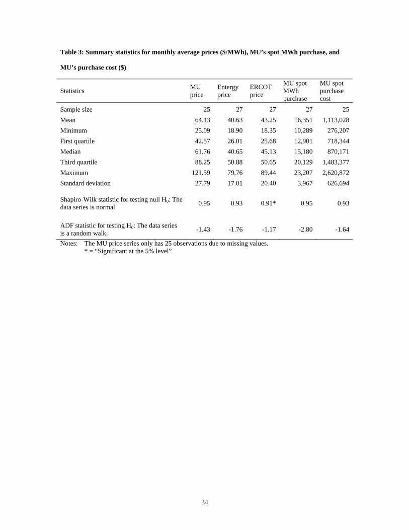
Table 3: Summary statistics for monthly average prices ($/MWh), MU’s spot MWh purchase, and

MU’s purchase cost ($)

Statistics MU price

Entergy price

ERCOT price

MU spot MWh purchase

MU spot purchase cost

Sample size 25 27 27 27 25 Mean 64.13 40.63 43.25 16,351 1,113,028 Minimum 25.09 18.90 18.35 10,289 276,207 First quartile 42.57 26.01 25.68 12,901 718,344 Median 61.76 40.65 45.13 15,180 870,171 Third quartile 88.25 50.88 50.65 20,129 1,483,377 Maximum 121.59 79.76 89.44 23,207 2,620,872 Standard deviation 27.79 17.01 20.40 3,967 626,694

Shapiro-Wilk statistic for testing null H0: The data series is normal 0.95 0.93 0.91* 0.95 0.93

ADF statistic for testing H0: The data series is a random walk. -1.43 -1.76 -1.17 -2.80 -1.64

Notes: The MU price series only has 25 observations due to missing values. * = “Significant at the 5% level”

34

Table 4: Spot price regression results

Independent Variable Coefficient

Intercept 4.10 Entergy price 0.80* ERCOT price 0.70* Adjusted R2 0.84 Mean squared error 127

ADF statistic for testing H0:The price series drift apart without limit -5.4*

Note: * = “Significant at the 5% level”

35