energy gradients in combined fragment molecular orbital and polarizable continuum model (fmo/pcm)...

Energy Gradients in Combined Fragment Molecular

Orbital and Polarizable Continuum Model

(FMO/PCM) Calculation

HUI LI,1DMITRI G. FEDOROV,

2TAKESHI NAGATA,

2KAZUO KITAURA,

2,3JAN H. JENSEN,

4MARK S. GORDON

5

1Department of Chemistry, University of Nebraska-Lincoln, Lincoln, Nebraska 685882National Institute of Advanced Industrial Science and Technology, 1-1-1 Umezono, Tsukuba,

Ibaraki 305-8568, Japan3Graduate School of Pharmaceutical Sciences, Kyoto University, Sakyo-ku,

Kyoto 606-8501, Japan4Department of Chemistry, University of Copenhagen, 2100 Copenhagen, Denmark

5Ames Laboratory, US-DOE and Department of Chemistry,Iowa State University, Ames, Iowa 50011

Received 27 October 2008; Revised 15 May 2009; Accepted 21 May 2009DOI 10.1002/jcc.21363

Published online 30 June 2009 in Wiley InterScience (www.interscience.wiley.com).

Abstract: The analytic energy gradients for the combined fragment molecular orbital and polarizable continuum

model (FMO/PCM) method are derived and implemented. Applications of FMO/PCM geometry optimization to

polyalanine show that the structures obtained with the FMO/PCM method are very close to those obtained with the

corresponding full ab initio PCM methods. FMO/PCM (RHF/6-31G* level) is used to optimize the solution structure

of the 304-atom Trp-cage miniprotein and the result is in agreement with NMR experiments. The key factors deter-

mining the relative stability of the a-helix, b-turn and the extended form in solution are elucidated for polyalanine.

q 2009 Wiley Periodicals, Inc. J Comput Chem 31: 778–790, 2010

Key words: fragment molecular orbital; polarizable continuum model; geometry optimization; polyalanine;

Trp-cage miniprotein; solution structure

Introduction

The fragment molecular orbital (FMO) method, developed by

Kitaura et al., is an ab initio based method that is able to treat

large systems of thousands of atoms.1 The distinctive feature of

FMO2,3 is the inclusion of the electrostatic field from the whole

system in each individual fragment calculation, and the use of the

systematic many-body expansion4 to incorporate interfragment

interactions. The fragment calculations are performed by self-con-

sistently polarizing the system, which is very important for highly

polar systems, such as proteins. Many common wave function

types have been incorporated into FMO,5–12 and the excited state

time-dependent density functional theory energy can also be com-

puted in gas phase and solution.13 Geometry optimizations14 and

molecular dynamics15,16 simulations can be performed with FMO,

and the method has been applied to a large number of processes

such as protein-ligand binding,17–19 protein-DNA interactions,20

explicit solvation,21,22 enzymatic reactions,23 excited states in

proteins24–26 and zeolite adsorption.27

Although considerable theoretical work has been invested

in developing computationally feasible methods for large

systems28–38 (see also refs. 39 and 40 for a review) in the gas phase,

few options are available for large solvated systems.41–46 As almost

all biological processes occur in solution, it is necessary to include

solvent effects in calculations on biological molecules. Continuum

solvent models are important computational methods for theoreti-

cal studies of condensed phase chemistry.47 In a continuum model

the solvent is treated as a dielectric medium while the solute is rep-

resented by a distribution of charges. The polarizable continuum

models (the earlier D-PCM48 and the recent Integral Equation For-

malism PCM, or IEF-PCM49), the conductor-like screening models

(COSMO50 and GCOSMO51 or conductor-like polarizable contin-

uum model, CPCM52,53 as its specific variant), the SS(V)PE54,55

Contract/grant sponsors: University of Nebraska-Lincoln, JSPS, Next

Generation SuperComputing Project, Nanoscience Program (MEXT,

Japan), Danish Research Agency; USA National Science Foundation

Petascale Applications grant

Correspondence to: H. Li; e-mail: [email protected] or D. G. Fedorov;

e-mail: [email protected]

q 2009 Wiley Periodicals, Inc.

models, as well as the SMxmodels,56 are popular continuum solva-

tion models.

An interface of FMO with the polarizable continuum model

(PCM) was developed for single point energy calculations.57

Geometry optimization of large biological molecules in solution

phase is also necessary because the solvent effects on the struc-

ture are usually very large. For example, salt bridges formed on

the surface of a protein usually dissociate in solution. Therefore,

gas phase geometry optimizations are not very meaningful for

studies of protein properties in solution. In this work, the

analytic energy gradients for the combined FMO/PCM method

are implemented and used for polypeptide and protein geometry

optimizations. The PCM has already been parallelized and

implemented to perform large-scale calculations for large biolog-

ical molecules.44,57 The combination of the FMO and PCM

methods, with fully functional energy gradients, will signifi-

cantly enhance the ab initio study of biological molecules.

The article is organized as follows. First, the PCM, FMO and

FMO/PCM methods are reviewed. Second, the theory and the

implementation of the FMO/PCM gradients are presented.

Finally the computational details and numerical results for a few

representative molecular systems are presented and discussed.

Theory

Polarizable Continuum Models

In both the PCM and conductor-like screening models

(COSMO) the solute molecule occupies a cavity in a bulk

solvent treated as a polarizable medium with a dielectric con-

stant e. The induced charge on the cavity surface is used to

describe the electrostatic interaction between the solute and the

bulk solvent. To solve the electrostatic boundary equation (i.e.

the Poisson equation) the continuous charge distribution on the

surface is divided into point charges at the centers of a finite

number of boundary surface elements, called tesserae. The

induced surface charges, denoted as a vector q, can be associ-

ated with the solute electrostatic potentials at the tesserae,

denoted as a vector V, by a matrix equation,

Cq ¼ �V ) q ¼ �C�1V (1)

where C is a geometric matrix whose elements differ depending

on the tessellation methods and various continuum model for-

malisms. In this article, the Polarizable Continuum Models (both

IEF-PCM49 and CPCM52,53) and RHF (including density func-

tional theory methods based on RHF type wave functions) are

considered. Although implemented within the IEF-PCM frame,

the CPCM should be regarded as a specific variant of the con-

ductor-like screening models (COSMO).50

The electrostatic interaction between the solute and the bulk

solvent, referred to as the PCM energy G, is defined as follows:

G ¼ 1

2VTq ¼ 1

2qTV ¼ � 1

2VTðC�1ÞTV ¼ � 1

2VTC�1V (2)

Based on the last expression of G in eq. (2), the first deriva-

tive of the PCM energy with respect to an atomic coordinate

x is [note that the standard equality (C21)x 5 2C21CxC21 is

used]:

Gx ¼ � 1

2ðVTÞxC�1V� 1

2VTðC�1ÞxV� 1

2VTC�1Vx

¼ 1

2ðVTÞxqþ 1

2VTC�1CxC�1V� 1

2VTC�1Vx

¼ 1

2ðVTÞxq� 1

2VTC�1Cxq� 1

2VTC�1Vx ð3Þ

Define

q ¼ �ðC�1ÞTV (4)

Equation (3) can be written as:

Gx ¼ 1

2ðVTÞxqþ 1

2ðqÞTCxqþ 1

2ðqÞTVx

¼ 1

2ðVTÞxðqþ qÞ þ 1

2ðqÞTCxq ð5Þ

If C is not symmetric (such as in the IEF-PCM method), q is

different from q. The evaluation of q requires a computational

cost similar to q. In the conductor-like screening model

(COSMO) and its specific variant CPCM, the matrix C is

symmetric, so

Gx ¼ ðVTÞxqþ 1

2qTCxq (6)

For IEF-PCM, eq. (6) can also be used as a good approxima-

tion.

The first term (VT)xq on the right side of eq. (6) represents

the (negative) forces on the PCM induced charges q in the

electrostatic field (VT)x created by the solute; the second term

(1/2)qTCxq represents the (negative) forces on the induced

charges in the electrostatic field created by other induced

charges and has a general expression such as q1q2/r212 when the

Cx matrix elements are explicitly written out. Due to the dis-

crete tessellation scheme used for numerical solution of the

Poisson boundary equation in PCM, neither the PCM energy

nor the gradients are continuous functions of the atomic

coordinates. However, using the GEPOL-AS and the variable-

tessera-number (VTN) approximations, nearly continuous IEF-

PCM and CPCM energy and gradients can be obtained, and

molecular geometry optimizations can be routinely

performed.53

The total nuclear gradients of a molecule are the sum of the

solvation energy gradients and the ‘‘gas phase’’ gradients. The

solute can be described either with classic electrostatic models

or various levels of quantum chemical models, or combined mo-

lecular mechanics and quantum mechanics models.58 For quan-

tum mechanical models, the RHF (or RHF based DFT) wave

function is determined variationally in the presence of the PCM

779Energy Gradients of FMO/PCM

Journal of Computational Chemistry DOI 10.1002/jcc

induced charges, and the ‘‘gas phase’’ nuclear gradients of the

solute molecule can be evaluated with the wave function deter-

mined in the presence of PCM charges.

It is common to perform empirical calculations together with

PCM to determine the free energy of cavitation of the solvent

(Gcav), free energies of dispersion (Gdis) and repulsion (Grep)

between the solute and the solvent.59,60 We denote the sum of these

energies by Gcdr. These three free energy terms depend only on the

geometrical parameters of the solute cavity and the predetermined

molecular mechanical interaction parameters, which are independ-

ent of the electronic state in the ab initio calculation. Since the

computational cost is relatively low for these molecular mechanical

calculations, a procedure has been implemented to numerically cal-

culate the gradients by displacing each coordinate separately by

1.03 1026 Bohr and then calculating the energy differences.53

FMO Method

The central idea of the FMO method is to break down a large

molecular system into many small fragments (also called mono-

mers), and perform feasible ab initio calculations for the frag-

ments and their combinations (e.g., dimers and trimers) in the

presence of other monomers. For the dimer-level FMO, that is

FMO2, the total energy of a large system is defined as:

E ¼XN

I

EI þXN

I>J

ðEIJ � EI � EJÞ (7)

where I and J run over all of the N fragments; EI is the SCF energy

of the Ith fragment in the external Coulomb field of the other N-1fragments; EIJ is the SCF energy of the I 1 J fragment pair

(dimer) in the external Coulomb field of the other N-2 fragments.

The computational procedure for the gas phase dimer-level

FMO (FMO2) is:

(a) Perform SCF calculations for the N fragments in the external

Coulomb fields of the other N-1 fragments, starting from

some initial guess of the electron density for each fragment.

(b) Repeat step (a) until all EI are converged.

(c) Perform SCF calculations for the close pairs of fragments

(dimers), in the external Coulomb fields of the N-2 frag-

ments; for far separated pairs the electrostatic interaction

approximation61 is used.

(d) Calculate E using eq. (7).

All of the other FMO2 properties can be defined similarly to

the energy. For example, the FMO2 energy gradient with respect

to a coordinate x is:

Ex ¼XN

I

ExI þ

XN

I>J

ðExIJ � Ex

I � ExJÞ (8)

Currently, the gradient calculation in the FMO method

includes the external Coulomb field derivative and is very close

to being analytic.62 Strictly speaking, one needs to add the

derivatives of the internal dimer energies [which are EIJ in

eq. (7) with the external Coulomb field subtracted] with respect

to the external monomer coordinates, since dimer calculations

are not fully variational with respect to the external monomer

density change; these terms contribute very little to the gradients

though, as the derivatives of the external Coulomb field itself

are computed.

FMO/PCM Method

An FMO/PCM calculation is similar to a full ab initio PCM

calculation: a molecular cavity is constructed for the solute (the

whole system instead of the FMO fragments) and tessellated.

The main difference is that in a full ab initio PCM calculation,

the solute potential V is determined directly from the total elec-

tron density, while in an FMO/PCM calculation V is determined

with the fragment potentials (e.g., VI and VIJ) that have been

computed from the fragment electron densities (note that V, VI,

and VIJ are vectors of the same size, given by the total number

of tesserae for the whole system). For example, V at the dimer

level is [c.f. eqs. (7) and (8)]:

V ¼XN

I

VI þXN

I>J

ðVIJ � VI � VJÞ (9)

The PCM solvent effect has been incorporated into the

FMO2 calculations at three levels. In FMO2/PCM[1], the PCM

is incorporated in the FMO2 scheme only at the monomer level

calculation: the PCM induced surface charges are determined

self-consistently with the monomer electron density in steps (a)

and (b) of the FMO2 procedure presented above. FMO2 dimer

calculations [steps (c) and (d)] are performed in the presence of

the PCM surface charges q determined at the monomer level.

There is a small cost for solving the PCM charges in the FMO2/

PCM[1] calculations, and the accuracy in the solvation energies

of polyalanine up to 40 residues is about 1–10 kcal/mol com-

pared to full ab initio RHF/PCM.57 FMO/PCM has been applied

to some interesting systems.63,64

In FMO2/PCM[1(2)], charges q are determined in the FMO2

scheme at the dimer level, but only once. After performing

FMO2/PCM[1], the PCM potential V is recomputed at the dimer

level with eq. (9), and used to solve for induced PCM surface

charges q. Then a new FMO2 iteration [all of the steps (a), (b),

(c) and (d)] is carried out in the presence of the fixed PCM

induced charges q. Thus, the cost of FMO2/PCM[1(2)] is nearly

double that of FMO/PCM[1], and the accuracy in the solvation

energies of polyalanine up to 40 residues is about 0–1.5 kcal/

mol compared to full ab initio RHF/PCM.57

In FMO2/PCM,2 the charges q are determined and incorpo-

rated into the FMO2 scheme at the dimer level calculation, and

iterated for �10 times to self-consistency. After each FMO2 cal-

culation [all steps (a), (b), (c) and (d)], PCM potentials V and

charges q are computed at the dimer level with eq. (9), and are

used for the next FMO2 calculation. Thus the cost of FMO/

PCM[2] is �10 times larger than that of FMO2/PCM[1], and the

accuracy is comparable to that of FMO2/PCM[1(2)]. The latter

is our recommended level for the energy calculations.

780 Li et al. • Vol. 31, No. 4 • Journal of Computational Chemistry


In all of the FMO2/PCM methods, the total energy of the

system is defined as:

E ¼XN

I

EI þXN

I>J

ðEIJ � EI � EJÞ � 1

2VTC�1Vþ Gcdr (10)

where EI, EJ, and EIJ are the FMO monomer and dimer ‘‘gas

phase’’ energies determined with the wave functions optimized

in the presence of the PCM surface charges. Clearly, due to the

two-body expansion in FMO and its interface with PCM, the

total energy obtained from eq. (10) is not truly variational. The

Gcdr term is independent of the ab initio method and is deter-

mined according to the molecular structure of the whole system.

At the size of polyalanine with 10 residues (112 atoms) there is

little time saving in doing an FMO calculation at the RHF level

compared to full ab initio. Due to the nearly linear scaling,

FMO offers a speed advantage for larger sizes.2 The PCM part

in the FMO/PCM method has a similar cost to that of full abinitio, because in FMO one treats the whole cavity in all frag-

ment calculations.

FMO/PCM Gradients

Similar to eq. (6), the total energy gradient for FMO2/PCM is

given by:

Ex ¼XN

I

ExI þ

XN

I>J

ðExIJ � Ex

I � ExJÞ þ ðVTÞxqþ 1

2qTCxqþ Gx

cdr

¼XN

I

ExI þ

XN

I>J

ðExIJ � Ex

I � ExJÞ þ

XN

I

ðVTI Þxq

þXN

I>J

½ðVTIJÞxq� ðVT

I Þxq� ðVTJ Þxq� þ

1

2qTCxqþ Gx

cdr ð11Þ

where ExI , E

xJ , and Ex

IJ are the FMO monomer and dimer ‘‘gas

phase’’ nuclear gradients determined with the wave functions

optimized in the presence of the PCM surface charges. Of

course, the evaluation of the FMO2/PCM gradients is performed

after the energy calculation in which the FMO2 wave function

and the PCM charges are determined.

Approximations are used to evaluate eq. (11): the same

approximations used for gas phase FMO2 gradients are adapted

for the FMO2 gradients in the FMO2/PCM interface by simply

using the wave function determined with the presence of the

PCM charges q, and the VTN53 approximation for full ab initioPCM gradients are adapted for the PCM in the FMO2/PCM

interface. The gradients for the cavitation, dispersion and repul-

sion terms (Gxcdr) for the FMO2/PCM method can be calculated

numerically using the same procedure described above.

Computational Methodology

The RHF/6-31G*, RHF/CPCM/6-31G* and FMO2-RHF/

CPCM[1]/6-31G* methods were used for geometry optimization

calculations with the criterion that the root mean square gradient

be smaller than 1024 au. In the solvated 1L2Y calculations,

diffuse functions (corresponding to the 6-311G* basis set) were

added to the two carboxyl groups. Some single point MP2 ener-

gies were calculated, based on the CPCM perturbed RHF wave

function, as proposed by Cammi.65 The gas phase optimized

structures of polyalanine were taken from previous work.14

In the authors’ experience, FMO and fully ab initio energy

curves follow each other quite closely, shifted by some value

related to the many-body charge transfer, exchange-repulsion

and their coupling.27,66 In this article the numerical accuracy of

the structures obtained with FMO2/PCM[1] is illustrated and

compared in detail. The energetics can be improved with FMO2/

PCM[1(2)], which is shown to have about a 1–2 kcal/mol

error.57

In all of the CPCM calculations, the simplified united-atom

radii (C 5 2.124 A, N 5 2.016 A, and O 5 1.908 A, no radius

for H) were used for molecular cavity construction with no

additional spheres. The GEPOL-AS tessellation scheme was

used with 240 initial tesserae per sphere. The solvent was

water with e 5 78.39. The apparent surface charges were deter-

mined by a semi-iterative DIIS procedure44,67 with no charge

renormalization.

In the FMO calculations reported here for polypeptides and

proteins, one residue per fragment division was always used. We

used the default calculation accuracy in FMO, and raised the

corresponding ab initio thresholds to match it. The threshold for

the FMO point charge approximation of the external Coulomb

field61 was changed from 2.0 to 2.5, to obtain better accuracy

for the FMO gradients.

Calculations were performed with the quantum chemistry

software package GAMESS,68,69 in which the FMO/PCM

method was implemented, and parallelized with the General

Distributed Data Interface, or GDDI.70 A Pentium4 cluster, with

34 3.2 GHz Pentium4 nodes equipped with 2 GB memory and

connected by Gigabit Ethernet, was used. For a timing example,

the calculation on the extended form of polyalanine with 10

residues, required 21.1, 10.9, and 19.1 min for MP2/CPCM,

FMO2-MP2/CPCM[1(2)] and FMO3-MP2/CPCM[1(2)], respec-

tively (single point energy).

Results and Discussion

Water Trimer (H2O)3

The FMO2 (gas phase and CPCM) and ab initio CPCM

gradients are approximations. Table 1 presents a detailed com-

parison between the numerical gradients and the approximate

analytic gradients for a cyclic water trimer (optimized at the

RHF/6-31G* level, Fig. 1) obtained at the various FMO2/CPCM

levels and RHF/CPCM methods. The total molecular energies

are also presented in Table 1 for comparison.

Despite its simplicity, water is more difficult to describe with

FMO than most bonded systems because it has significant

charge transfer. The FMO errors are mostly caused by the inter-

fragment charge transfer, rather than the detached bonds them-

selves.27,66

Table 1 clearly shows that the FMO2/CPCM energies differ

from the RHF/CPCM energy by �0.3 kcal/mol (this error is

caused by three-body quantum-mechanical effects, involving



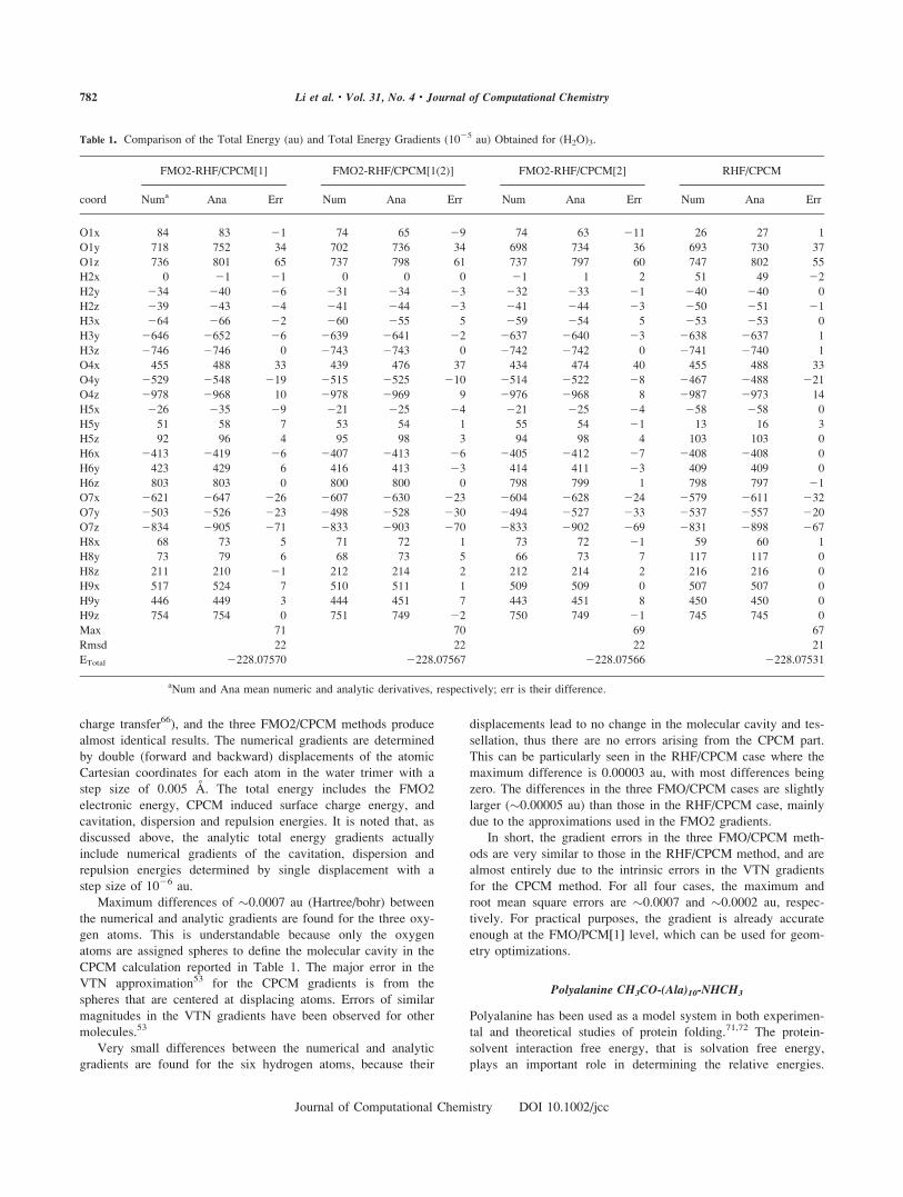
charge transfer66), and the three FMO2/CPCM methods produce

almost identical results. The numerical gradients are determined

by double (forward and backward) displacements of the atomic

Cartesian coordinates for each atom in the water trimer with a

step size of 0.005 A. The total energy includes the FMO2

electronic energy, CPCM induced surface charge energy, and

cavitation, dispersion and repulsion energies. It is noted that, as

discussed above, the analytic total energy gradients actually

include numerical gradients of the cavitation, dispersion and

repulsion energies determined by single displacement with a

step size of 1026 au.

Maximum differences of �0.0007 au (Hartree/bohr) between

the numerical and analytic gradients are found for the three oxy-

gen atoms. This is understandable because only the oxygen

atoms are assigned spheres to define the molecular cavity in the

CPCM calculation reported in Table 1. The major error in the

VTN approximation53 for the CPCM gradients is from the

spheres that are centered at displacing atoms. Errors of similar

magnitudes in the VTN gradients have been observed for other

molecules.53

Very small differences between the numerical and analytic

gradients are found for the six hydrogen atoms, because their

displacements lead to no change in the molecular cavity and tes-

sellation, thus there are no errors arising from the CPCM part.

This can be particularly seen in the RHF/CPCM case where the

maximum difference is 0.00003 au, with most differences being

zero. The differences in the three FMO/CPCM cases are slightly

larger (�0.00005 au) than those in the RHF/CPCM case, mainly

due to the approximations used in the FMO2 gradients.

In short, the gradient errors in the three FMO/CPCM meth-

ods are very similar to those in the RHF/CPCM method, and are

almost entirely due to the intrinsic errors in the VTN gradients

for the CPCM method. For all four cases, the maximum and

root mean square errors are �0.0007 and �0.0002 au, respec-

tively. For practical purposes, the gradient is already accurate

enough at the FMO/PCM[1] level, which can be used for geom-

etry optimizations.

Polyalanine CH3CO-(Ala)10-NHCH3

Polyalanine has been used as a model system in both experimen-

tal and theoretical studies of protein folding.71,72 The protein-

solvent interaction free energy, that is solvation free energy,

plays an important role in determining the relative energies.

Table 1. Comparison of the Total Energy (au) and Total Energy Gradients (1025 au) Obtained for (H2O)3.

FMO2-RHF/CPCM[1] FMO2-RHF/CPCM[1(2)] FMO2-RHF/CPCM[2] RHF/CPCM

coord Numa Ana Err Num Ana Err Num Ana Err Num Ana Err

O1x 84 83 21 74 65 29 74 63 211 26 27 1

O1y 718 752 34 702 736 34 698 734 36 693 730 37

O1z 736 801 65 737 798 61 737 797 60 747 802 55

H2x 0 21 21 0 0 0 21 1 2 51 49 22

H2y 234 240 26 231 234 23 232 233 21 240 240 0

H2z 239 243 24 241 244 23 241 244 23 250 251 21

H3x 264 266 22 260 255 5 259 254 5 253 253 0

H3y 2646 2652 26 2639 2641 22 2637 2640 23 2638 2637 1

H3z 2746 2746 0 2743 2743 0 2742 2742 0 2741 2740 1

O4x 455 488 33 439 476 37 434 474 40 455 488 33

O4y 2529 2548 219 2515 2525 210 2514 2522 28 2467 2488 221

O4z 2978 2968 10 2978 2969 9 2976 2968 8 2987 2973 14

H5x 226 235 29 221 225 24 221 225 24 258 258 0

H5y 51 58 7 53 54 1 55 54 21 13 16 3

H5z 92 96 4 95 98 3 94 98 4 103 103 0

H6x 2413 2419 26 2407 2413 26 2405 2412 27 2408 2408 0

H6y 423 429 6 416 413 23 414 411 23 409 409 0

H6z 803 803 0 800 800 0 798 799 1 798 797 21

O7x 2621 2647 226 2607 2630 223 2604 2628 224 2579 2611 232

O7y 2503 2526 223 2498 2528 230 2494 2527 233 2537 2557 220

O7z 2834 2905 271 2833 2903 270 2833 2902 269 2831 2898 267

H8x 68 73 5 71 72 1 73 72 21 59 60 1

H8y 73 79 6 68 73 5 66 73 7 117 117 0

H8z 211 210 21 212 214 2 212 214 2 216 216 0

H9x 517 524 7 510 511 1 509 509 0 507 507 0

H9y 446 449 3 444 451 7 443 451 8 450 450 0

H9z 754 754 0 751 749 22 750 749 21 745 745 0

Max 71 70 69 67

Rmsd 22 22 22 21

ETotal 2228.07570 2228.07567 2228.07566 2228.07531

aNum and Ana mean numeric and analytic derivatives, respectively; err is their difference.



Three conformers of CH3CO-(Ala)10-NHCH3, that is a-helix,b-turn and the extended form (see Fig. 2), were optimized with

the gas phase RHF/6-31G*, RHF/CPCM/6-31G* and FMO2-

RHF/CPCM[1]/6-31G* methods.

Table 2 presents the root mean square deviation (RMSD)

between some representative geometrical parameters optimized

using gas phase RHF/6-31G* and RHF/CPCM/6-31G*, and

those between RHF/CPCM/6-31G* and FMO2-RHF/CPCM[1]/

6-31G*, for the three conformers. For each conformer, the com-

parisons are made at the structure superposition that minimizes

the RMSD of the Cartesian coordinates (r in Table 2).

The RMSD of all the atoms (All atom r in Table 2) between

the gas phase RHF/6-31G* and RHF/CPCM/6-31G* optimized

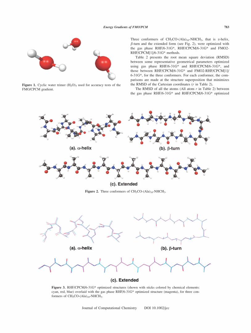
Figure 1. Cyclic water trimer (H2O)3 used for accuracy tests of the

FMO/CPCM gradient.

Figure 2. Three conformers of CH3CO-(Ala)10-NHCH3.

Figure 3. RHF/CPCM/6-31G* optimized structures (shown with sticks colored by chemical elements:

cyan, red, blue) overlaid with the gas phase RHF/6-31G* optimized structure (magenta), for three con-

formers of CH3CO-(Ala)10-NHCH3.



geometries are 0.297, 0.115, and 0.211 A, respectively, for the

three conformers, while those between the RHF/CPCM/6-31G*

and FMO2-RHF/CPCM[1]/6-31G* optimized geometries are

only 0.030, 0.048, and 0.026 A, respectively. Similar values and

changes can be seen for the heavy atoms. The RMSD of the 110

bond lengths (l in Table 2) between the gas phase RHF/6-31G*

and RHF/CPCM/6-31G* optimized geometries are 0.0042,

0.0038, and 0.0040 A, respectively, for the a-helix, b-turn and

extended conformers. As expected, smaller bond length RMSD

values are found between RHF/CPCM/6-31G* and FMO2-RHF/

CPCM[1]/6-31G* optimized geometries, implying that these two

geometries are similar to each other. The situation for the

RMSD in the bond angles and dihedral angles is similar to that

for the bond lengths.

The solvent effects upon the structure are the strongest in the

a-helix (Table 2 and Fig. 3), which is likely to be related to its

large dipole moment and thus large electrostatic interaction with

the solvent. The b-turn is fairly rigid due to its intramolecular

hydrogen bonds (which are retained upon solvation), so its struc-

ture changes little. The extended form overall is the least affected

upon solvation, despite the fact that it has the largest solvation

energy. This is better seen numerically in Table 2, where the first

three entrees compare RHF and RHF/CPCM; one can note that

the apparently larger deviation for the extended form is because

of the different scale (see Fig. 3) used to demonstrate the change

in the angles from residue to residue; the absolute values of the

angle changes is mostly the smallest for the extended form.

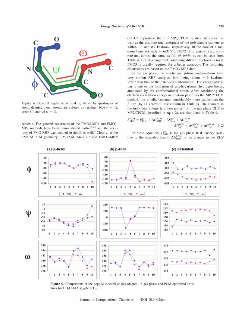
The dihedral angles in their standard biochemical definition

describe the relative orientation of adjacent pairs of amino acid

residues: / describes torsion about the N-Ca bond; x describes

torsion about the C1-N bond; w describes torsion about the Ca-C1

bond (see Fig. 4). Figure 5 shows the dihedral angles /, x, andw(in the gas phase and in solution phase. For the a-helix, the larg-est deformation upon solvation is for the three dihedral angles

around the 10th peptide bonds (between ALA-10 and the

��NHCH3 cap); it can be seen in Figure 5 that the ��NHCH3

group has the largest deviation from gas phase. For the b-turn, onthe contrary, the solvation effects are the largest for the middle

(turn) part, dihedral angles around the 4th, 5th, 6th, and 7th pep-

tide bonds (see Fig. 5). For the extended form interestingly the

whole structure is almost uniformly affected. Also, for all three

isomers one can observe the following general trend: / and xbecome more positive while w becomes more negative upon sol-

vation.

The accuracy of FMO/CPCM verses the fully ab initioCPCM can be seen in Table 2. The deviation is very small:

0.026-0.046 A over all coordinates, and 0.001-0.002 A and 0.23-

0.30 degree in bond lengths and angles, respectively. The dihe-

dral angles are reproduced by FMO with an error of about 0.75–

2.27 degrees.

Table 3 presents the H��O distances in the N��H��O¼¼C

hydrogen bonds in the a-helix and b-turn conformers optimized

using the three methods. On going from gas phase RHF/6-31G*

to solution phase RHF/CPCM/6-31G*, d1, d2, d7, d8, d9 of the

a-helix, d1, d3, d8, and d10 of the b-turn become slightly

shorter (by 0.05–0.1 A); d4 and d5 of the a-helix become signif-

icantly shorter (by �0.3 A); d3, d6 of the a-helix and d5 of the

b-turn become slightly longer (by 0.05–0.1 A). The differences

between the H��O distances obtained with RHF/CPCM/6-31G*

and FMO2-RHF/CPCM[1]/6-31G* methods are relatively small.

A maximum difference of 0.1 A is observed for d5 of the b-turn, while the others are all around or below 0.02 A. These dif-

ferences are very similar to those in gas phase.14 In general, the

FMO2/CPCM[1] results can be considered to be a very good

approximation to the full ab initio RHF/CPCM result.

One of the main questions in such a polyalanine study is

what are the relative energies of various structures such as the

a-helix, random coil, b-turn and unfolded conformations? To an-

swer this question requires the calculation of the electron corre-

lation energy.73 Second-order perturbation theory (MP2) calcula-

tions were performed for the three conformations of interest

here, and the results are presented in Table 4.

It is well known that the geometries are less sensitive than

the energies to the level of theory in quantum chemical calcula-

tions, and accurate higher-level single point energy calculations

on lower-level (but still acceptable) optimized geometries are

Table 2. RMSD of the Geometric Parametersa Optimized for CH3CO-(Ala)10-NHCH3 and Trp-Cage

Miniprotein 1L2Y.

Structure All atom r (A) Heavy atom r (A) l (A) h (deg) / (deg) w (deg) x (deg)

a-Helixb 0.297 0.268 0.0042 0.44 8.67 8.59 1.56

b-Turnb 0.115 0.101 0.0038 0.41 3.86 4.22 2.30

Extendedb 0.211 0.103 0.0040 0.60 1.93 4.99 1.72

a-Helixc 0.030 0.028 0.0014 0.23 1.41 1.39 0.88

b-Turnc 0.046 0.048 0.0021 0.30 1.40 2.27 2.08

Extendedc 0.026 0.026 0.0014 0.21 0.75 1.28 1.06

1L2Yd 2.156 2.026 0.0049 1.12 11.30 14.02 4.05

1L2Ye 1.107 1.013 0.0116 1.71 12.05 15.78 6.19

ar represents the Cartesian coordinate RMSD, l and h represent the covalent bond length and angle RMSD,

respectively. /, w, and x represent peptide dihedral angles.14

bDifference between gas phase RHF/6-31G* and RHF/CPCM/6-31G*.cDifference between RHF/CPCM/6-31G* and FMO2-RHF/CPCM[1]/6-31G*.dDifference between gas phase FMO2-RHF/6-31G* and FMO2-RHF/CPCM[1]/6-31G*.eDifference between the first model (NMR derived) in 1L2Y and FMO2-RHF/CPCM[1]/6-31G*.



sensible. The general accuracies of the FMO2-MP2 and FMO3-

MP2 methods have been demonstrated earlier5,74 and the accu-

racy of FMO-RHF was studied in detail as well.4 Clearly, at the

FMO2/CPCM geometry, FMO2-MP2/6-31G* and FMO3-MP2/

6-31G* reproduce the full MP2/CPCM relative stabilities (as

well as the absolute total energies) of the polyalanine isomers to

within 1.1 and 0.7 kcal/mol, respectively. In the case of a me-

dium basis set such as 6-31G*, FMO2 is in general very accu-

rate and almost the same as full ab initio, as can be seen from

Table 4. But if a larger set containing diffuse functions is used,

FMO3 is usually required for a better accuracy. The following

discussions are based on the FMO3-MP2 data.

In the gas phase, the a-helix and b-turn conformations have

very similar RHF energies, both being about 213 kcal/mol

lower than that of the extended conformation. The energy lower-

ing is due to the formation of amide-carbonyl hydrogen bonds,

attenuated by the conformational strain. After considering the

electron correlation energy in solution phase via the MP2/CPCM

method, the a-helix becomes considerably more stable than the

b-turn (by 14 kcal/mol: last column in Table 4). The changes in

the individual energy terms on going from the gas phase RHF to

MP2/CPCM, described in eq. (12), are also listed in Table 4.

EPCMMP2 ¼ Egas

RHF þ DGPCMRHF þ DEgas

corr þ DGPCMcorr

þ DGPCMcav þ DGPCM

disp þ DGPCMrep ð12Þ

In these equations EgasRHF is the gas phase RHF energy (rela-

tive to the extended form); DGPCMRHF is the change in the RHF

Figure 4. Dihedral angles /, w, and x, shown by quadruples of

atoms defining them. Atoms are colored by residues: blue (i 2 1),

green (i) and red (i 1 1).

Figure 5. Comparisons of the peptide dihedral angles (degree) in gas phase and PCM optimized struc-

tures for CH3CO-(Ala)10-NHCH3.



energy on going from the gas phase to solution phase (including

the CPCM electrostatic solvation energy); DEgascorr is the gas phase

MP2 correlation energy (relative to the extended form); DGPCMcorr

is the change in the MP2 correlation energy on going from the

gas phase to solution phase; DGPCMcav , DGPCM

disp and DGPCMrep are the

cavitation, and the solvent-solute dispersion and repulsion ener-

gies, respectively, which are independent of the ab initio elec-

tronic state. EPCMMP2 is the MP2/CPCM energy, relative to the gas

phase MP2 energy of the extended form.

Not surprisingly, the extended conformation gains more sol-

vation energy due to its larger surface as compared to the a-he-lix and b-turn. For example, the stabilizations (DGPCM

RHF ) for the

extended, b-turn and a-helix conformations are 267.7, 255.8,

and 260.4 kcal/mol, respectively; the solvent-solute dispersion

interaction DGPCMdisp for the extended, b-turn and a-helix confor-

mations are 2107.4, 289.1, and 287.7 kcal/mol, respectively.

However, the more compact b-turn and a-helix conformations

gain more electron correlation energy (DEgascorr) than the extended

form; 225.6 and 216.0, respectively, relative to the extended

form. The intramolecular solute dispersion energy change due to

solvation DGPCMcorr is quite similar in all three isomers (9–10 kcal/

mol). The cavitation energy and the repulsion terms are slightly

more positive for the extended form, compared to the other two

isomers, which is also a reflection of its larger volume and

surface.

On going from gas phase RHF to MP2/CPCM, the energy of

the a-helix relative to the extended form becomes even lower

due to a net gain in stability [220.6 kcal/mol, see Table 4],

while for the b-turn, the relative energy becomes higher due to a

net loss in stability (213.3 vs. 26.5 kcal/mol). In other words,

the solvent (water) stabilizes the a-helix most, and the b-turnleast, with the extended form between them.

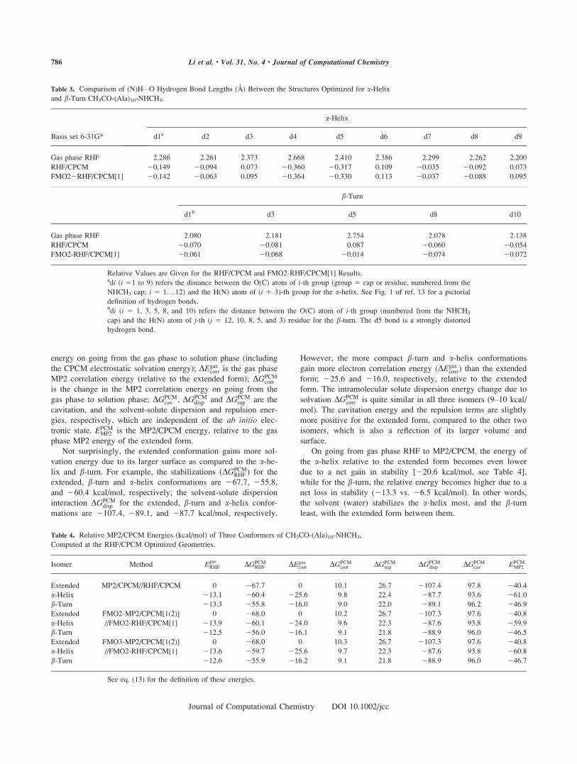
Table 3. Comparison of (N)H��O Hydrogen Bond Lengths (A) Between the Structures Optimized for a-Helixand b-Turn CH3CO-(Ala)10-NHCH3.

Basis set 6-31G*

a-Helix

d1a d2 d3 d4 d5 d6 d7 d8 d9

Gas phase RHF 2.286 2.261 2.373 2.668 2.410 2.386 2.299 2.262 2.200

RHF/CPCM 20.149 20.094 0.073 20.360 20.317 0.109 20.035 20.092 0.073

FMO22RHF/CPCM[1] 20.142 20.063 0.095 20.364 20.330 0.113 20.037 20.088 0.095

b-Turn

d1b d3 d5 d8 d10

Gas phase RHF 2.080 2.181 2.754 2.078 2.138

RHF/CPCM 20.070 20.081 0.087 20.060 20.054

FMO2-RHF/CPCM[1] 20.061 20.068 20.014 20.074 20.072

Relative Values are Given for the RHF/CPCM and FMO2-RHF/CPCM[1] Results.adi (i 51 to 9) refers the distance between the O(C) atom of i-th group (group 5 cap or residue, numbered from the

NHCH3 cap; i 5 1. . .12) and the H(N) atom of (i 1 3)-th group for the a-helix. See Fig. 1 of ref. 13 for a pictorial

definition of hydrogen bonds.bdi (i 5 1, 3, 5, 8, and 10) refers the distance between the O(C) atom of i-th group (numbered from the NHCH3

cap) and the H(N) atom of j-th (j 5 12, 10, 8, 5, and 3) residue for the b-turn. The d5 bond is a strongly distorted

hydrogen bond.

Table 4. Relative MP2/CPCM Energies (kcal/mol) of Three Conformers of CH3CO-(Ala)10-NHCH3,

Computed at the RHF/CPCM Optimized Geometries.

Isomer Method EgasRHF DGPCM

RHF DEgascorr DGPCM

corr DGPCMrep DGPCM

disp DGPCMcav EPCM

MP2

Extended MP2/CPCM//RHF/CPCM 0 267.7 0 10.1 26.7 2107.4 97.8 240.4

a-Helix 213.1 260.4 225.6 9.8 22.4 287.7 93.6 261.0

b-Turn 213.3 255.8 216.0 9.0 22.0 289.1 96.2 246.9

Extended FMO2-MP2/CPCM[1(2)] 0 268.0 0 10.2 26.7 2107.3 97.6 240.8

a-Helix //FMO2-RHF/CPCM[1] 213.9 260.1 224.0 9.6 22.3 287.6 93.8 259.9

b-Turn 212.5 256.0 216.1 9.1 21.8 288.9 96.0 246.5

Extended FMO3-MP2/CPCM[1(2)] 0 268.0 0 10.3 26.7 2107.3 97.6 240.8

a-Helix //FMO2-RHF/CPCM[1] 213.6 259.7 225.6 9.7 22.3 287.6 93.8 260.8

b-Turn 212.6 255.9 216.2 9.1 21.8 288.9 96.0 246.7

See eq. (13) for the definition of these energies.



It is interesting to observe that the correlation energy (or the

intramolecular dispersion in solute) is decreased in solution.

This was also observed earlier65 for very different systems and

thus may be a general trend. The orbital energy levels can shed

some light on this. In all isomers, occupied orbitals are stabi-

lized and virtual orbitals are destabilized on going from gas

phase to solution. The occupied orbital stabilization is easy to

understand: solvent adds an electrostatic interaction to the Fock

matrix, which lowers the orbital energies; the virtual orbitals

adjust to this change by a corresponding increase in their orbital

energies. The MP2 correlation energy65 can be represented as

the coupling term (two-electron integrals) divided by the sum of

two virtual-occupied orbital energy differences. An inspection of

the orbital energies shows that the solvent increases the HOMO-

LUMO gap by 0.0017, 0.105, and 0.0145 hartree (or 11.0, 65.7,

and 9.1 kcal/mol), in the extended form, a-helix and b-turn,respectively. Larger orbital energy differences lead to a smaller

(less negative) intramolecular dispersion energy in solution. It is

also interesting that a rather large change in the a-helix HOMO-

LUMO gap (which is brought about by its large dipole moment)

does not incur a much smaller change in the dispersion energy

(see DGPCMcorr in Table 4). This may be related to a reduced

orbital delocalization in solution, which was also observed

earlier,13 resulting in larger coupling matrix elements in the

correlation energy expression.

The data in Table 4 are computed at the CPCM optimized

geometries, and the terms in Table 5 add the deformation energy

due to the differences between the gas phase and solution opti-

mized structures. DG0solv defines the total direct solvation energy

of each isomer separately (CPCM minus gas phase, at the

CPCM geometry), and is computed by summing the relevant

data in Table 4,

DG0solv ¼ DGPCM

RHF þ DGPCMcorr þ DGPCM

rep þ DGPCMdisp þ DGPCM

cav (13)

DGsolv gives the actual solvation energy (for the solvation

process from the gas phase optimized structure),

DGsolv ¼ DG0solv þ DEdef

RHF þ DEdefcorr (14)

DEdefRHF and DEdef

corr are the deformation energy components

(RHF and MP2 correlation energy, respectively). They provide

an energy criterion for how much the structures change upon

solvation. The deformation energies are normally positive, as the

energies are evaluated in the gas phase, and the CPCM structure

has a higher gas phase energy, which is indeed observed at the

RHF level. The correlation contribution is negative, indicating

that the CPCM structure has a larger dispersion energy (despite

the weakening of the intramolecular dispersion due to solvent, at

the same geometry), because the CPCM structure is more com-

pact. Ideally, the structures should be optimized at the MP2

level (not currently feasible), in which case the total deformation

energy, DEdefelec 1 DEdef

corr, would most likely be positive (destabi-

lization).

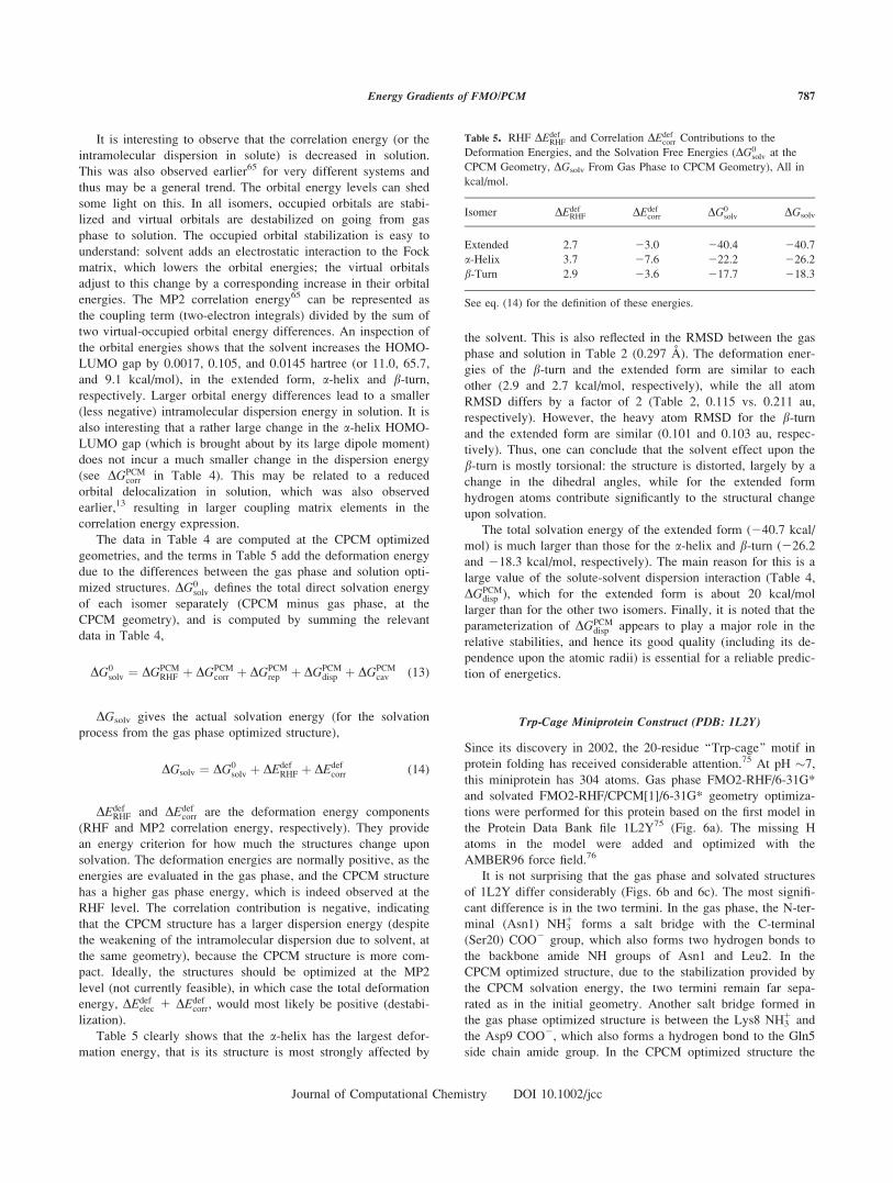
Table 5 clearly shows that the a-helix has the largest defor-

mation energy, that is its structure is most strongly affected by

the solvent. This is also reflected in the RMSD between the gas

phase and solution in Table 2 (0.297 A). The deformation ener-

gies of the b-turn and the extended form are similar to each

other (2.9 and 2.7 kcal/mol, respectively), while the all atom

RMSD differs by a factor of 2 (Table 2, 0.115 vs. 0.211 au,

respectively). However, the heavy atom RMSD for the b-turnand the extended form are similar (0.101 and 0.103 au, respec-

tively). Thus, one can conclude that the solvent effect upon the

b-turn is mostly torsional: the structure is distorted, largely by a

change in the dihedral angles, while for the extended form

hydrogen atoms contribute significantly to the structural change

upon solvation.

The total solvation energy of the extended form (240.7 kcal/

mol) is much larger than those for the a-helix and b-turn (226.2

and 218.3 kcal/mol, respectively). The main reason for this is a

large value of the solute-solvent dispersion interaction (Table 4,

DGPCMdisp ), which for the extended form is about 20 kcal/mol

larger than for the other two isomers. Finally, it is noted that the

parameterization of DGPCMdisp appears to play a major role in the

relative stabilities, and hence its good quality (including its de-

pendence upon the atomic radii) is essential for a reliable predic-

tion of energetics.

Trp-Cage Miniprotein Construct (PDB: 1L2Y)

Since its discovery in 2002, the 20-residue ‘‘Trp-cage’’ motif in

protein folding has received considerable attention.75 At pH �7,

this miniprotein has 304 atoms. Gas phase FMO2-RHF/6-31G*

and solvated FMO2-RHF/CPCM[1]/6-31G* geometry optimiza-

tions were performed for this protein based on the first model in

the Protein Data Bank file 1L2Y75 (Fig. 6a). The missing H

atoms in the model were added and optimized with the

AMBER96 force field.76

It is not surprising that the gas phase and solvated structures

of 1L2Y differ considerably (Figs. 6b and 6c). The most signifi-

cant difference is in the two termini. In the gas phase, the N-ter-

minal (Asn1) NH31 forms a salt bridge with the C-terminal

(Ser20) COO2 group, which also forms two hydrogen bonds to

the backbone amide NH groups of Asn1 and Leu2. In the

CPCM optimized structure, due to the stabilization provided by

the CPCM solvation energy, the two termini remain far sepa-

rated as in the initial geometry. Another salt bridge formed in

the gas phase optimized structure is between the Lys8 NH31 and

the Asp9 COO2, which also forms a hydrogen bond to the Gln5

side chain amide group. In the CPCM optimized structure the

Table 5. RHF DEdefRHF and Correlation DEdef

corr Contributions to the

Deformation Energies, and the Solvation Free Energies (DG0solv at the

CPCM Geometry, DGsolv From Gas Phase to CPCM Geometry), All in

kcal/mol.

Isomer DEdefRHF DEdef

corr DG0solv DGsolv

Extended 2.7 23.0 240.4 240.7

a-Helix 3.7 27.6 222.2 226.2

b-Turn 2.9 23.6 217.7 218.3

See eq. (14) for the definition of these energies.



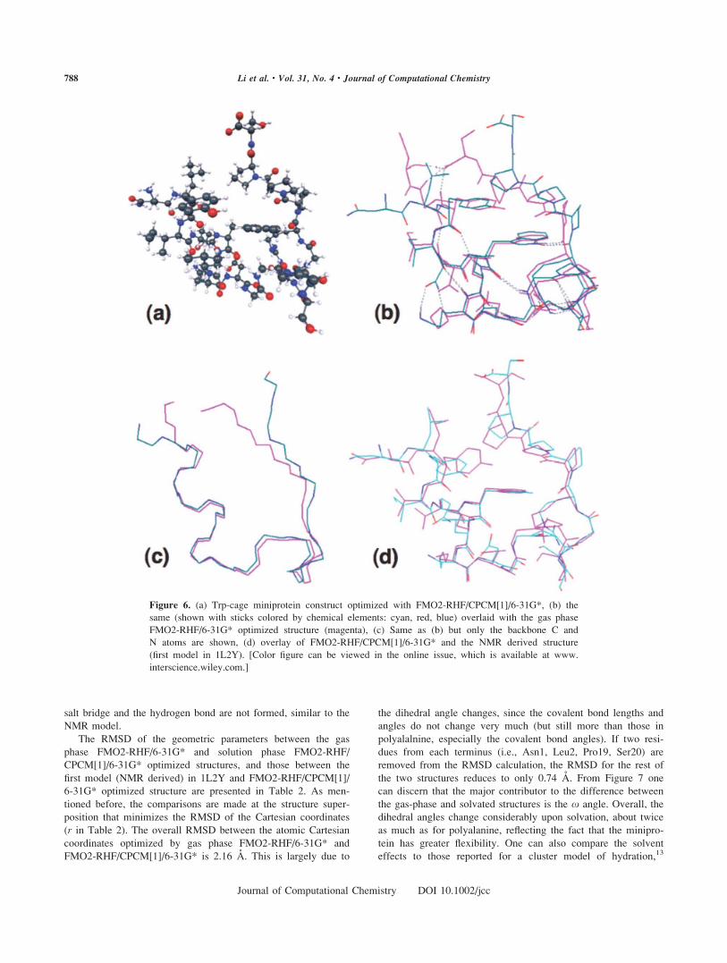
salt bridge and the hydrogen bond are not formed, similar to the

NMR model.

The RMSD of the geometric parameters between the gas

phase FMO2-RHF/6-31G* and solution phase FMO2-RHF/

CPCM[1]/6-31G* optimized structures, and those between the

first model (NMR derived) in 1L2Y and FMO2-RHF/CPCM[1]/

6-31G* optimized structure are presented in Table 2. As men-

tioned before, the comparisons are made at the structure super-

position that minimizes the RMSD of the Cartesian coordinates

(r in Table 2). The overall RMSD between the atomic Cartesian

coordinates optimized by gas phase FMO2-RHF/6-31G* and

FMO2-RHF/CPCM[1]/6-31G* is 2.16 A. This is largely due to

the dihedral angle changes, since the covalent bond lengths and

angles do not change very much (but still more than those in

polyalalnine, especially the covalent bond angles). If two resi-

dues from each terminus (i.e., Asn1, Leu2, Pro19, Ser20) are

removed from the RMSD calculation, the RMSD for the rest of

the two structures reduces to only 0.74 A. From Figure 7 one

can discern that the major contributor to the difference between

the gas-phase and solvated structures is the x angle. Overall, the

dihedral angles change considerably upon solvation, about twice

as much as for polyalanine, reflecting the fact that the minipro-

tein has greater flexibility. One can also compare the solvent

effects to those reported for a cluster model of hydration,13

Figure 6. (a) Trp-cage miniprotein construct optimized with FMO2-RHF/CPCM[1]/6-31G*, (b) the

same (shown with sticks colored by chemical elements: cyan, red, blue) overlaid with the gas phase

FMO2-RHF/6-31G* optimized structure (magenta), (c) Same as (b) but only the backbone C and

N atoms are shown, (d) overlay of FMO2-RHF/CPCM[1]/6-31G* and the NMR derived structure

(first model in 1L2Y). [Color figure can be viewed in the online issue, which is available at www.

interscience.wiley.com.]



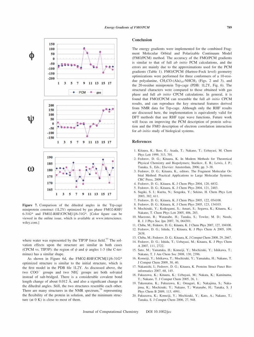
where water was represented by the TIP3P force field.77 The sol-

vation effects upon the structure are similar in both cases

(CPCM vs. TIP3P): the region of / and w angles 1-3 (the C-ter-

minus) has a similar shape.

As shown in Figure 6d, the FMO2-RHF/CPCM[1]/6-31G*

optimized structure is similar to the initial structure, which is

the first model in the PDB file 1L2Y. As discussed above, the

two COO2 groups and two NH31 groups are both solvated

instead of salt-bridged. There is a considerable covalent bond

length change of about 0.012 A, and also a significant change in

the dihedral angles. Still, the two structures resemble each other.

There are many structures in the NMR spectrum,75 representing

the flexibility of the protein in solution, and the minimum struc-

ture (at 0 K) is close to most of them.

Conclusion

The energy gradients were implemented for the combined Frag-

ment Molecular Orbital and Polarizable Continuum Model

(FMO/PCM) method. The accuracy of the FMO/PCM gradients

is similar to that of full ab initio PCM calculations, and the

errors are mainly due to the approximations used for the PCM

gradients (Table 1). FMO/CPCM (Hartree-Fock level) geometry

optimizations were performed for three conformers of a 10-resi-

due polyalanine, CH3CO-(Ala)10-NHCH3 (Figs. 2 and 3), and

the 20-residue miniprotein Trp-cage (PDB: 1L2Y, Fig. 6). The

structural characters were compared to those obtained with gas

phase and full ab initio CPCM calculations. In general, it is

found that FMO/CPCM can resemble the full ab initio CPCM

results, and can reproduce the key structural features derived

from NMR data for Trp-cage. Although only the RHF results

are discussed here, the implementation is equivalently valid for

DFT methods that use RHF type wave functions. Future work

will focus on improving the PCM description of protein solva-

tion and the FMO description of electron correlation interaction

for ab initio study of biological systems.

References

1. Kitaura, K.; Ikeo, E.; Asada, T.; Nakano, T.; Uebayasi, M. Chem

Phys Lett 1999, 313, 701.

2. Fedorov, D. G.; Kitaura, K. In Modern Methods for Theoretical

Physical Chemistry and Biopolymers; Starikov, E. B.; Lewis, J. P.;

Tanaka, S., Eds.; Elsevier: Amsterdam, 2006; pp. 3–38.

3. Fedorov, D. G.; Kitaura, K., editors. The Fragment Molecular Or-

bital Method: Practical Applications to Large Molecular Systems;

CRC Press, 2009.

4. Fedorov, D. G.; Kitaura, K. J Chem Phys 2004, 120, 6832.


6. Sugiki, S. I.; Kurita, N.; Sengoku, Y.; Sekino, H. Chem Phys Lett

2003, 382, 611.



9. Mochizuki, Y.; Koikegami, S.; Amari, S.; Segawa, K.; Kitaura, K.;

Nakano, T. Chem Phys Lett 2005, 406, 283.

10. Maezono, R.; Watanabe, H.; Tanaka, S.; Towler, M. D.; Needs,

R. J. J Phys Soc Jpn 2007, 76, 064301.

11. Chiba, M.; Fedorov, D. G.; Kitaura, K. J Chem Phys 2007, 127, 104108.

12. Fedorov, D. G.; Ishida, T.; Kitaura, K. J Phys Chem A 2005, 109,

2638.

13. Chiba, M.; Fedorov, D. G.; Kitaura, K. J Comput Chem 2008, 29, 2667.

14. Fedorov, D. G.; Ishida, T.; Uebayasi, M.; Kitaura, K. J Phys Chem

A 2007, 111, 2722.

15. Sato, M.; Yamataka, H.; Komeiji, Y.; Mochizuki, Y.; Ishikawa, T.;

Nakano, T. J Am Chem Soc 2008, 130, 2396.

16. Komeiji, Y.; Ishikawa, T.; Mochizuki, Y.; Yamataka, H.; Nakano, T.

J Comput Chem 2009, 30, 40.

17. Nakanishi, I.; Fedorov, D. G.; Kitaura, K. Proteins Struct Funct Bio-

informatics 2007, 68, 145.

18. Fukuzawa, K.; Kitaura, K.; Uebayasi, M.; Nakata, K.; Kaminuma,

T.; Nakano, T. J Comput Chem 2005, 26, 1.

19. Takematsu, K.; Fukuzawa, K.; Omagari, K.; Nakajima, S.; Naka-

jima, K.; Mochizuki, Y.; Nakano, T.; Watanabe, H.; Tanaka, S. J

Phys Chem B 2009, 113, 4991.

20. Fukuzawa, K.; Komeiji, Y.; Mochizuki, Y.; Kato, A.; Nakano, T.;

Tanaka, S. J Comput Chem 2006, 27, 948.

Figure 7. Comparison of the dihedral angles in the Trp-cage

miniprotein construct (1L2Y) optimized by gas phase FMO2-RHF/

6-31G* and FMO2-RHF/CPCM[1]/6-31G*. [Color figure can be

viewed in the online issue, which is available at www.interscience.

wiley.com.]



21. Komeiji, Y.; Ishida, T.; Fedorov, D. G.; Kitaura, K. J Comput Chem

2007, 28, 1750.

22. Mochizuki, Y.; Komeiji, Y.; Ishikawa, T.; Nakano, T.; Yamataka, H.

Chem Phys Lett 2007, 437, 66.

23. Ishida, T.; Fedorov, D. G.; Kitaura, K. J Phys Chem B 2006, 110,

1457.

24. Mochizuki, Y.; Nakano, T.; Amari, S.; Ishikawa, T.; Tanaka, K.;

Sakurai, M.; Tanaka, S. Chem Phys Lett 2007, 433, 360.

25. Ikegami, T.; Ishida, T.; Fedorov, D. G.; Kitaura, K.; Inadomi, Y.;

Umeda, H.; Yokokawa, M.; Sekiguchi, S. J Comput Chem [Epub

ahead of print: DOI 10.1002/jcc.21272].

26. Taguchi, N.; Mochizuki, Y.; Nakano, T.; Amari, S.; Fukuzawa, K.;

Ishikawa, T.; Sakurai, M.; Tanaka, S. J Phys Chem B 2009, 113,

1153.

27. Fedorov, D. G.; Jensen, J. H.; Deka, R. C.; Kitaura, K. J Phys Chem

A 2008, 112, 11808.

28. Imamura, A.; Aoki, Y.; Maekawa, K. J Chem Phys 1991, 95, 5419.

29. Yang, W. Phys Rev Lett 1991, 66, 1438.

30. Aoki, Y.; Suhai, S.; Imamura, A. Int J Quantum Chem 1994, 52, 267.

31. Gao, J. L.; Truhlar, D. G. Ann Rev Phys Chem 2002, 53, 467.

32. Zhang, D. W.; Zhang, J. Z. H. J Chem Phys 2003, 119, 3599.

33. Babu, K.; Gadre, S. R. J Comput Chem 2003, 24, 484.

34. Nikitina, E.; Sulimov, V.; Zayets, V.; Zaitseva, N. Int J Quantum

Chem 2004, 97, 747.

35. Makowski, M.; Korchowiec, J.; Gu, F. L.; Aoki, Y. J Comput Chem

2006, 27, 1603.

36. Paulus, B. Phys Reports-Rev Sec Phys Lett 2006, 428, 1.

37. Inaba, T.; Sato, F. J Comput Chem 2007, 28, 984.

38. Huang, L.; Massa, L.; Karle, J. Proc Natl Acad Sci USA 2008, 105,

1849.

39. Fedorov, D. G.; Kitaura, K. J Phys Chem A 2007, 111, 6904.

40. Gordon, M. S.; Mullin, J. M.; Pruitt, S. R.; Roskop, L. B.;

Slipchenko, L. V.; Boatz, J. A. J Phys Chem B (in press).

41. Rega, N.; Cossi, M.; Barone, V. Chem Phys Lett 1998, 293, 221.

42. York, D. M.; Lee, T.-S.; Yang, W. J Am Chem Soc 1996, 118,

10940.

43. Scalmani, G.; Barone, V.; Kudin, K. N.; Pomelli, C. S.; Scuseria,

G. E.; Frisch, M. J. Theor Chem Acc 2004, 111, 90.

44. Li, H.; Pomelli, C. S.; Jensen, J. H. Theor Chem Acc 2003, 109, 71.

45. Mei, Y.; Ji, C. G.; Zhang, J. Z. H. J Chem Phys 2006, 125, 094906.

46. Bondesson, L.; Rudberg, E.; Luo, Y.; Salek, P. J Phys Chem B

2007, 111, 10320.

47. Tomasi, J.; Mennucci, B.; Cammi, R. Chem Rev 2005, 105, 2999.

48. Miertus, S.; Scrocco, E.; Tomasi, J. Chem Phys 1981, 55, 117.

49. Cances, E.; Mennucci, B.; Tomasi, J. J Chem Phys 1997, 107, 3032.

50. Klamt, A.; Schuurmann, G. J Chem Soc Perkin Trans 2 1993, 799.

51. Truong, T. N.; Stefanovich, E. V. Chem Phys Lett 1995, 240, 253.

52. Barone, V.; Cossi, M. J Phys Chem A 1998, 102, 1995.

53. Li, H.; Jensen, J. H. J Comput Chem 2004, 25, 1449.

54. Chipman, D. M. Theor Chem Acc 2002, 107, 80.

55. Chipman, D. M.; Dupuis, M. Theor Chem Acc 2002, 107, 90.

56. Marenich, A. V.; Olson, R. M.; Kelly, C. P.; Cramer, C. J.; Truhlar,

D. G. J Chem Theory Comput 2007, 3, 2011.

57. Fedorov, D. G.; Kitaura, K.; Li, H.; Jensen, J. H.; Gordon, M. S.

J Comput Chem 2006, 27, 976.

58. Barone, V.; Improta, R.; Rega, N. Theor Chem Acc 2004, 111, 237.

59. Pierotti, R. A. Chem Rev 1976, 76, 717.

60. Floris, F. M.; Tomasi, J.; Ahuir, J. L. P. J Comput Chem 1991, 12, 784.

61. Nakano, T.; Kaminuma, T.; Sato, T.; Fukuzawa, K.; Akiyama, Y.;

Uebayasi, M.; Kitaura, K. Chem Phys Lett 2002, 351, 475.

62. Nagata, T.; Fedorov, D. G.; Kitaura, K. Chem Phys Lett 2009, 475,

124.

63. He, X.; Fusti-Molnar, L.; Cui, G. L.; Merz, K. M. J Phys Chem B

2009, 113, 5290.

64. Sawada, T.; Fedorov, D. G.; Kitaura, K. Int J Quantum Chem 2009,

109, 2033.

65. Cammi, R.; Mennucci, B.; Tomasi, J. J Phys Chem A 1999, 103,

9100.

66. Fedorov, D. G.; Kitaura, K. J Comput Chem 2007, 28, 222.

67. Pomelli, C. S.; Tomasi, J.; Barone, V. Theor Chem Acc 2001, 105,

446.

68. Schmidt, M. W.; Baldridge, K. K.; Boatz, J. A.; Elbert, S. T.;

Gordon, M. S.; Jensen, J. H.; Koseki, S.; Matsunaga, N.; Nguyen,

K. A.; Su, S. J.; Windus, T. L.; Dupuis, M.; Montgomery, J. A.

J Comput Chem 1993, 14, 1347.

69. Gordon, M. S.; Schmidt, M. W. In Theory and applications of

computational chemistry; Dykstra, C. E.; Frenking, G.; Kim, K. S.;

Scuseria, G. E., Eds.; Amsterdam: Elsevier, 2005.

70. Fedorov, D. G.; Olson, R. M.; Kitaura, K.; Gordon, M. S.; Koseki,

S. J Comput Chem 2004, 25, 872.

71. Peng, Y.; Hansmann, U. H. E. Biophys J 2002, 82, 3269.

72. van Giessen, A. E.; Straub, J. E. J Chem Phys 2005, 122, 024904.

73. Ozawa, T.; Okazaki, K. J Comput Chem 2008, 29, 2656.

74. Fedorov, D. G.; Ishimura, K.; Ishida, T.; Kitaura, K.; Pulay, P.;

Nagase, S. J Comput Chem 2007, 28, 1476.

75. Neidigh, J. W.; Fesinmeyer, R. M.; Andersen, N. H. Nat Struct Biol

2002, 9, 425.

76. Cornell, W. D.; Cieplak, P.; Bayly, C. I.; Gould, I. R.; Merz, K. M.;

Ferguson, D. M.; Spellmeyer, D. C.; Fox, T.; Caldwell, J. W.;

Kollman, P. A. J Am Chem Soc 1995, 117, 5179.

77. Jorgensen, W. L.; Chandrasekhar, J.; Madura, J. D.; Impey, R. W.;

Klein, M. L. J Chem Phys 1983, 79, 926.



energy gradients in combined fragment molecular orbital and polarizable continuum model (fmo/pcm)...

Documents