ENERGY-224

Reservoir Simulation

Project Report

Ala Alzayer

Autumn Quarter

December 3, 2014

Contents

1 Objective 2

2 Governing Equations 2

3 Methodolgy 3

3.1 BlockMesh . . . . . . . . . . . . . . . . . . . . . . . . . . . . . . . . . . . . . . . . . 3

3.2 SnappyHexMesh . . . . . . . . . . . . . . . . . . . . . . . . . . . . . . . . . . . . . . 4

3.3 Boundary Conditions . . . . . . . . . . . . . . . . . . . . . . . . . . . . . . . . . . . . 4

4 Simulation Results 5

4.1 Convergence Study . . . . . . . . . . . . . . . . . . . . . . . . . . . . . . . . . . . . . 6

4.2 Permeability . . . . . . . . . . . . . . . . . . . . . . . . . . . . . . . . . . . . . . . . 8

4.3 Tortuosity . . . . . . . . . . . . . . . . . . . . . . . . . . . . . . . . . . . . . . . . . . 8

4.4 REV Study . . . . . . . . . . . . . . . . . . . . . . . . . . . . . . . . . . . . . . . . . 9

4.5 Scalability . . . . . . . . . . . . . . . . . . . . . . . . . . . . . . . . . . . . . . . . . . 11

5 Summary 12

6 References 12

1

1 Objective

The main objective of this project is to investigate some of the basic parameters computed in

a direct numerical simulation for a single phase fluid at the pore scale. My focus will be on the

velocity distribution in complex geometry and how it can be used to get an idea of average upscaled

quantities such as absolute permeability. I will examine the effects of the choice of simulation model

used on these properties.

2 Governing Equations

The governing equation for the fluid flow in the pore space will be the mass and momentum balance

equations of Navier-Stokes, which for an incompressible fluid (neglecting gravity) are:

∇·v = 0 (1)

ρ

(∂v

∂t+ v· ∇v

)= −∇p+ µ∇2v (2)

The usual algorithm of choice to solve the pressure-velocity relationship would be the Pressure

Implicit Operator-Splitting (PISO) algorithm (Issa, 1985). This is a predictor-corrector method

which can handle transient problems. Given that the Reynolds number (ratio of intertial to viscous

forces) for the flow in the medium under investigation � 1, we can neglect the intertial effects and

get a more simplified equation:

0 = −∇p+ µ∇2v (3)

This is referred to as the Stokes equation which is a steady-state formulation; for that reason

the Semi-Implicit Method for Pressure Linked Equations (SIMPLE) algorithm (Patankar, 1980)

will be ideal for iteratively guessing/correcting the pressure-velocity fields. This algorithm does not

solve transient problems but should be faster than the PISO algorithm in solving Stokes problems

which is the case in this study. In addition to the equations of motions, the boundary condition

for the fluid/solid interface, where the solid is represented by the grains, is needed. We will impose

the condition that the fluid at the surface of the grains will have a zero velocity relative to the

boundary, this is referred to as the no-slip condition.

2

3 Methodolgy

OpenFOAMr software will be the tool used to simulate the fluid flow in the pore space. The

main steps to solve these kinds of problems will be to discretize the domain (which is not a trivial

task) and set the desired initial and boundary conditions. After that we feed the problem to

the simpleFoam solver (which utilizes the SIMPLE algorithm) to obtain a converged velocity and

pressure field. I will elaborate on the discretization part next since it is more important than one

might think. The combination of tools used in OpenFOAMr to mesh complex geometries are

blockMesh, which defines the background grid, and snappyHexMesh, which alters the grid to fit

the void space being modeled. I will elaborate on the two steps below.

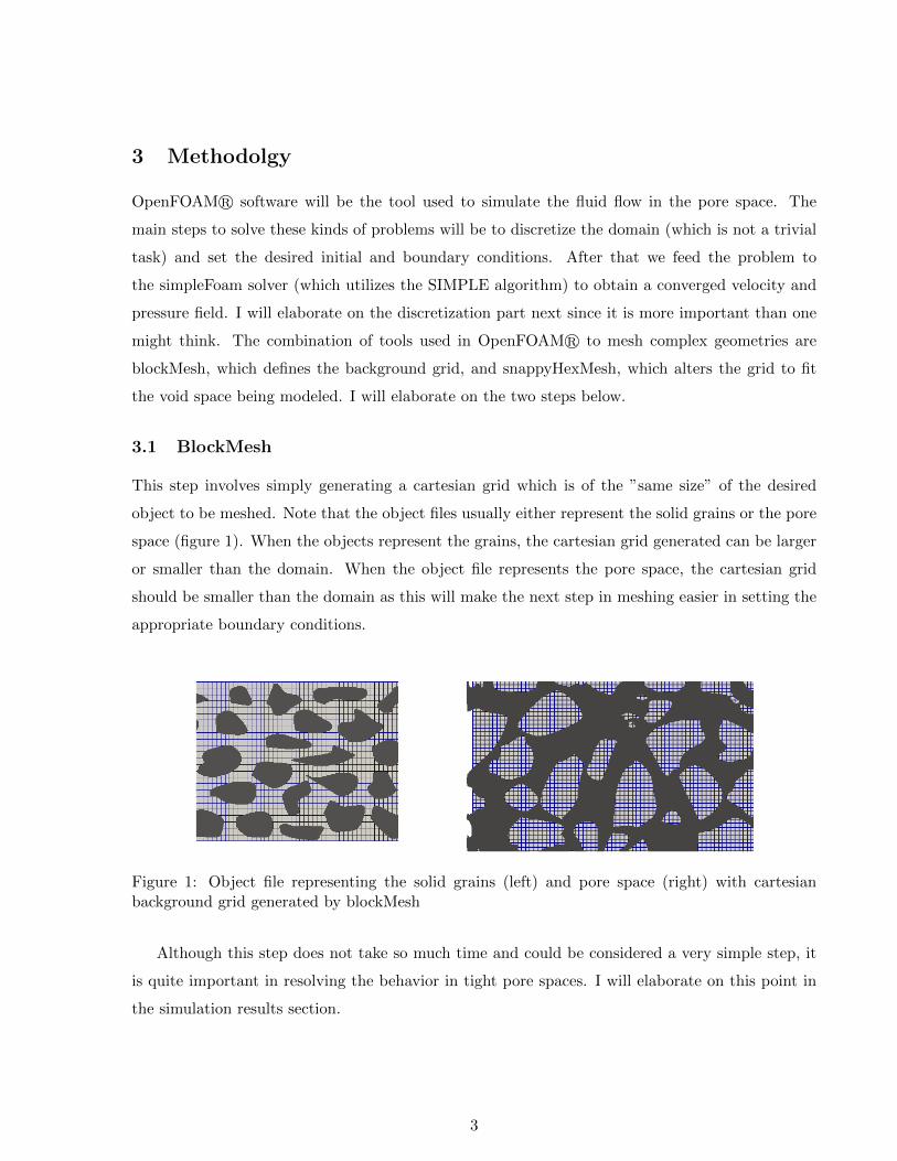
3.1 BlockMesh

This step involves simply generating a cartesian grid which is of the ”same size” of the desired

object to be meshed. Note that the object files usually either represent the solid grains or the pore

space (figure 1). When the objects represent the grains, the cartesian grid generated can be larger

or smaller than the domain. When the object file represents the pore space, the cartesian grid

should be smaller than the domain as this will make the next step in meshing easier in setting the

appropriate boundary conditions.

Figure 1: Object file representing the solid grains (left) and pore space (right) with cartesianbackground grid generated by blockMesh

Although this step does not take so much time and could be considered a very simple step, it

is quite important in resolving the behavior in tight pore spaces. I will elaborate on this point in

the simulation results section.

3

3.2 SnappyHexMesh

The next step after ensuring that the generated grid covers the desired domain involves cutting out

the grains. This will leave us with a mesh that only represents the pore space. The snappyHexMesh

tool does this in two steps as shown in figure 2. The first step involves removing the grid blocks

adjacent to the grains, the next step smoothens the edges and snaps the grid onto the surfaces of

the grains. The cells with faces touching the grains are all identified as an additional ”boundary”

in our domain to be specified.

Figure 2: The first (left) and second (right) step used in snappyHexMesh

This step is the more time consuming (as well as memory consuming) part of the meshing; the

snappyHexMesh step can take up to 12 hours on a single processor for a 2D sandstone image (0.6

mm × 1.83mm) and a cartesian grid with 3000×8000 cells.

3.3 Boundary Conditions

With the domain fully discretized, the only step left is to initialize the domain and set the boundary

conditions. The only constance we use is the kinematic viscosity of the fluid which in this case is

set to 1e-6 m2s−1. For the Stokes problem we are only concerned with velocity and pressure fields

and therefore initalize the internal domain with zero pressure and velocity, while the boundary

conditions are shown in Table 1 below.

Table 1: Boundary Conditions

Boundary Pressure [m2/s2] Velocity [m/s]

Inlet 1e-3 zero gradient

Outlet 0 zero gradient

Walls zero gradient 0 (no slip condition)

Grain Surfaces zero gradient 0 (no slip condition)

(Note: pressure is normalized by density)

4

4 Simulation Results

As mentioned before, with the domain discretized and initial/boundary conditions set, the sim-

pleFoam solver is used to iteratively guess/correct the pressure-velocity fields until convergence

(residual smaller than 1e-6). Since we are dealing with a steady state problem, the results will

include only the steady state pressure and velocity distributions which depend solely on the bound-

ary conditions and pore geometry. The two main geometries I am considering here are shown in

figure 3, I will refer to the one on the left as ”simple” case whereas the one on the right as ”SS2”

which is a sandstone slice used in the SUPRI-A group (courtesy of Soulaine). Both these models

are 2D slices of the pore geometry and therefore all simuations run are in the x-y plane. I am

showing the pressure distributions in both geometries which will practically be the same in all the

cases considered here. In the next part I will show the results of the convergence study done on

both these geometries which should highlight the importance of the grid used in modeling pore

scale flow.

Figure 3: Pressure distribution for simple (left) and SS2 (right) pore geometry

5

4.1 Convergence Study

The main parameters I am considering here are the average and maximum velocity of the domain

after convergence. I am normalizing the results for each case with that of the highest resolution

case (figure 4). Note the dashed black line which shows the number of pixels in the real image for

each geometry. We see that the significant difference in results are seen for any grid that has a

lower resolution than the actual image. After that we see that the simple geometry converges to

the solution faster than the SS2 case. This is expected as SS2 is much more complicated with a

wider distribution of pore throat sizes. This supports the current best practices which emphasizes

mesh quality even beyond the base image resolution (Soulaine, 2014). Ideally we would like to

capture the poiseuille flow regime in all the pore throats, which would require 5-10 cells resolution

atleast.

Figure 4: Convergence study of the simple (left) and the SS2 (right) geometry

One interesting observation here is that the average velocity seems to be more restrictive than

the maximum velocity, which is the opposite of what one would expect. However, when looking

at the velocity distribution in the different cases we see that the less resolved cases are capable of

capturing the high velocities in the small pore throats. On the other hand we see that due to the

low resolution the velocities can be overestimated in the large pores between the pore throats where

the high resolution model show more variation (figure 5). I included the 100×25 case just to show

the extreme case of when the grid resolution is less than the image size; we see a significant loss

of connectivity which should not even be considered a valid simulation model. Figure 6 shows the

same trend for the SS2 geometry. The significance of these results show the importance of having

a converged model especially when it comes to obtain effective parameters such as permeability.

6

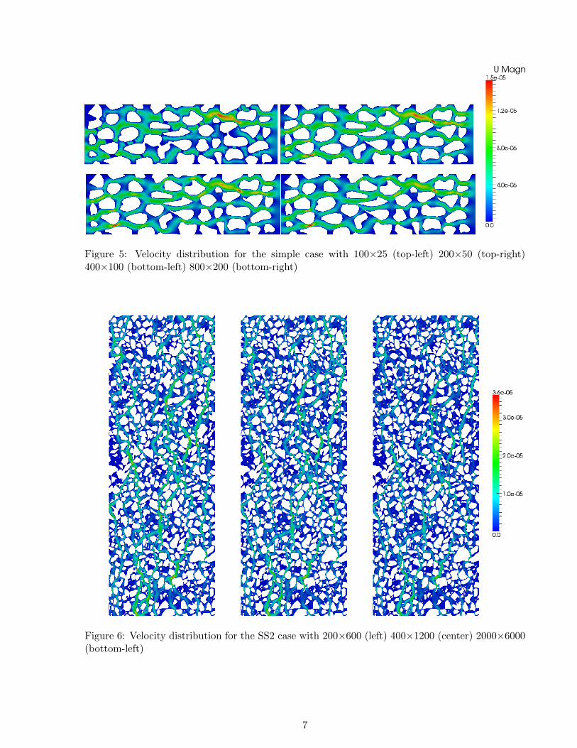
Figure 5: Velocity distribution for the simple case with 100×25 (top-left) 200×50 (top-right)400×100 (bottom-left) 800×200 (bottom-right)

Figure 6: Velocity distribution for the SS2 case with 200×600 (left) 400×1200 (center) 2000×6000(bottom-left)

7

4.2 Permeability

Absolute permeability is probably one of the most common effective parameters obtained from

direct numerical simulation at the pore scale. This is quite easy to do once an accurate velocity field

is obtained; previous section shows that caution needs to be taken when deciding that the model

being used is representative. Below I estimate the absolute permeabilities using the converged

models for the two geometries:

ksimple =µLx

∆P× 1

V

∫vvxdV =

(1e− 5)(9.2e− 4)(1.697e− 6)

(1e− 3)= 15.82 d

kss2 =µLy

∆P× 1

V

∫vvydV =

(1e− 5)(1.6e− 3)(1.28e− 6)

(1e− 3)= 20.75 d

If we use a less resolved model we can use an average velocity value that is 1.1 × the converged

value as seen in figure 4. This would result in permeabilities values of 17.4 and 22.83 darcies

respectively. This might not seem so severe for this case since the geometries being used, despite

being complex, are relatively homogeneous.

4.3 Tortuosity

Tortuosity is another average parameter which can be deduced from pore scale simulation. There

are relatively more sophisticated ways of computing the tortuosity of a medium by computing the

dispersion tensor. However, here an attempt was made to compute tortuosity using stream lines.

Once the velocity field is obtained we are able to trace particle paths (using the stream tracer

tool in ParaViewr). The simplest definition of tortuosity is the length of path traveled (length of

streamline) over the distance between the two points (length of domain). For this project, I only

traced 5 streamlines on the simple geometry case (figure 7) and took the average length of the 5

streamlines. This gives us an idea about the average tortuosity in this geometry:

τ =StreamlineLength

LengthofDomain=

0.1

0.092= 1.087

Ideally we would have a much larger number of streamlines to obtain a value which is more

representative. The next section will investigate the idea of a representative elementary volume

(REV) which plays an important role in estimating effective properties such as permeability and

tortuosity.

8

Figure 7: Variation of average porosity and speed (left) and the corresponding error (right) withincreasing sample size

4.4 REV Study

The use of effective properties such as porosity and permeability is based on the assumption that the

source of these averaged properties is statistically representative of the entire domain. The following

study is a simple investigation of the porosity and average velocity which could be considered as an

indication of permeability. This was conducted on a square domain obtained from stiching the SS2

geometery (Efros and Freeman, 2001). For this study a simulation was run on the whole domain

to obtain the velocity profile. The methodolgy presented was followed to make sure that we are

using a converged grid. We then used an averaging tool which can extract the results from a given

sample size of the domain and obtain the average porosity and velocity. A total of 24 samples were

taken from the domain; the results and relative errors compared to the full domain solution are

shown in Figure 8.

9

Figure 8: Variation of average porosity and speed (left) and the corresponding error (right) withincreasing sample size

If we assume that the sample size is considered an REV once the error is bounded by 2%

(arbitrary number), we can see that the two averaged properties differ in REV size (figure 8). This

confirms the well known idea that different averaged parameters might have different respective

REV sizes. Ideally the REV size should be representative of all required averaged parameters

(tortuosity, permeability, dispersion tensor...etc).

Figure 9: REV size for average porosity (left) and velocity (right) for a bounded error of 2%

10

4.5 Scalability

Despite the fact we are dealing with the millimeter scale, due to the size of the simulation grids

(O(107) cells) it is obvious how expensive these computations are. This brings us to concern

of computational speed where the importance of parallelizing comes into play. This is done in

OpenFOAMr by decomposing the full domain into multiple domains. These sub-domains are

then linked with one another through boundary conditions. Once the simulation are done the full

domain is reconstructed. The following strong scaling study was conducted on the SS2 geometry

with 1.92 million cells (figure 10).

Figure 10: Strong scaling for 1.92 million cell case showing speed up (left) and clock time (right)

From the results we can see that these simulation are scalable up to a point, which is expected.

We see that the speed up factor is almost a 1 to 1 relationship with the number of processors up to

64 processors where we see a deviation. That is exactly the point where each processor deals with

30,000 cells; which has been observed with OpenFOAMr to be the point where communication

time starts to counter the speed up resulting from decomposing the domain to multiple processors.

We also see the point at which we start to loose speed up (20,000 cells per processor).

11

5 Summary

Direct numerical simulation in complex geometry is a powerful tool for gaining insight of the

underlying physics of fluid flow in porous media, however care should be taken when dealing with

these models. We have highlighted the importance of the mesh starting from the background

cartesian grid, which could seem trivial. Having enough resolution to capture the flow in tight

pore throats is necessary for obtaining an accurate and representative overall velocity field, where

we saw that the average velocity is more restrictive than the maximum velocity with convergence.

The impact of that is seen in estimating effective properties such as absolute permeability.

Obtaining a REV is also a very important part of analyzing results from pore scale simulations.

In this study we looked at porosity and average velocity in a 2D relatively homogeneous sandstone.

This difference in REV size could be the case with other properties estimated which lie beyond the

scope of this study.

6 References

1. Issa. Solution of the implicitly discretised fluid flow equations by operator-splitting. Journal

of Computational Physics, 62:40-65, 1985.

2. Patankar. Numerical Heat Transfer And Fluid Flow. Taylor and Francis, 1980.

3. C. Soulaine notes on Direct numerical simulation in fully saturated porous media, 2014.

4. A.A. Efros and W.T. Freeman, ”Image Quilting for Texture Synthesis and Transfer,” Com-

puter Graphics (Proc. Siggraph 2001), ACM Press, New York, 2001, pp.341-346.

12