endogenous formation of financial dualism...
TRANSCRIPT

Hitotsubashi University Repository
Title Endogenous Formation of Financial Dualism
Author(s) Mallik, Rajlakshmi
Citation Hitotsubashi Journal of Economics, 48(2): 137-158
Issue Date 2007-12
Type Departmental Bulletin Paper
Text Version publisher
URL http://doi.org/10.15057/15183
Right

ENDOGENOUS FORMATION OF FINANCIAL DUALISM�
R6?A6@H=B> M6AA>@
NSHM Business School
Kolkata 700 053, India
Received August 2006; Accepted April 2007
Abstract
Starting with a given initial distribution of wealth holders (who are potential lenders) we
show the endogenous creation of financial dualism as experienced by many countries. As the
historic and contemporary country experiences suggest, the history of modern banking can be
traced back to the formation of the joint stock banks, which stand in contrast to the native
bankers. Typically the joint stock banks are initially formed by the local rich and attract
deposits and have a much broader area of operation, both geographically and across industries.
The depositors belong to the middle wealth segment. The native bankers on the other hand are
hardly ever in a position to receive deposits and typically consist of the small wealth holders
who continue to lend locally.
Key Words: Coalition, Diversification, Informal Lending, Joint Stock Bank, Risk Aversion,
Financial Dualism
JEL Classification: C72, G21, O17
I . Introduction
Why do we observe di#erent types of financial institutions in the credit markets of many
countries that are in their early phase of development?1 Why do indigenous banks consisting
of sole proprietorship and partnership firms co-exist with larger privately owned joint stock
commercial banks with a much larger capital base? The indigenous banks usually engage in
local lending while the joint stock banks constitute nation-wide network and have a much
broader area of operation both geographically and across industry. Again the joint stock banks
typically accept deposits, unlike the indigenous bankers. This raises the question, why is it that
some wealth holders prefer keeping deposits with banks for a fixed certain return, rather than
engaging in local banking like other wealth holders, or becoming share holders of the larger
joint stock bank?
� The author wishes to thank Prof. Abhirup Sarkar for valuable comments and suggestions. This paper has also
benefited from the comments of the participants at the seminars in Nottingham University, Keele University,
University of East Anglia and Cornell University. We thank two anonymous referees for their insightful comments
and suggestions, which has helped to improve the paper considerably. The usual disclaimer applies.1 For discussion on structure and issues pertaining to the credit markets in LDCs see Basu (1998).
Hitotsubashi Journal of Economics 48 (2007), pp.137-158. � Hitotsubashi University

These are some of the issues that this paper tries to address. The above observations find
historical and contemporary support in the country experiences of industrially advanced
countries like UK and Germany in their early stages of development in the 18th and 19th
centuries and India in the early 20th century.2 These countries saw modern banking develop in
the form of joint stock banks in the wake of legislative reforms as some of the private bankers
found it better to merge and take advantage of risk diversification instead of paying other
banks for investment services in other parts of the country. At the same time some of the
erstwhile wealth holders continued with their local lending operations.
In this paper we develop a static theoretical model that matches the country experiences
cited above. We consider an economy consisting of wealth holders with varying endowments
of an investment good and potential entrepreneurs with project plans. Each wealth holder has
a neighbouring entrepreneur about whose project he has complete information. The wealth
holders can invest in the neighbouring entrepreneur’s project (home project) or they can
diversify their portfolio by investing in other projects also. However he can not monitor the
other projects. To quote Deane (1979) writing on the economy of U.K. during the Industrial
Revolution, “Bankers often originated in industry or trade, or for example in the legal
profession...Often too, tax collectors became bankers. ...One of the consequences of this heteroge-
neous banking system was that when the pioneers of the industrial revolution went in search of
capital, they could hope to find local bankers who had access to enough personal knowledge about
the borrower on the one hand, and enough practical knowledge of the trade or industry concerned
on the other, to be able to take risks which a less personally involved banker would find
incalculable and therefore out of range.”
The only way the wealth holders can diversify is by colluding with the other wealth
holders through multilateral investments, which involve exchange of information among
wealth holders about their respective home projects. We assume that there is a court of law but
it is very costly in terms of time and expenses involved for an individual to move the court,
which makes unilateral diversification infeasible. Given that coalitions can be formed, other
isolated wealth holders may be tempted to keep deposits with these coalitions. Although
moving the court individually is costly, a group of depositors may still be able to take e#ective
advantage of the court of law. The formal model describing this economy is given in section
II.
In the context of such a model, which replicates a snapshot view of a traditional
economy,3 we show how financial dualism might emerge. We show the conditions that would
be conducive to the formation of the native system of banking, constituting the informal credit
market on the one hand along with the larger joint stock banks on the other.4 These joint stock
banks, unlike the indigenous bankers, are also deposit-taking institutions and are the forerun-
ners of the modern commercial banks constituting the formal credit market.
There is a large literature on sustainable coalition formation in the context of dynamic
models of repeated interaction. Some important contributions are Dutta et al. (1989),
2 Refer to Deane (1979), Kindleberger (1984) and Johnson (2000) for banking history of U.K. and Germany.
For India refer to Bhattacharya (1989) and Kaushal (1979). Also see Tun Wai (1956, 57).3 See Bhaduri (1977), Basu (1990) and Jain (1999) for the kind of economy being discussed here.4 There is a large literature on the endogenous growth of financial intermediation — i.e. how financial intermedi-
aries are formed endogenously (Ramkrishnan and Thakor, 1984). But we are not concerned with this issue, as this
does not distinguish between various types of financial intermediaries.
=>IDIHJ76H=> ?DJGC6A D; :8DCDB>8H [December+-2

Mookherjee and Ray (2001), Thomas and Worrall (1988), Coate and Ravallion (1993),
Kocherlakota (1996), Ligon, Thomas and Worrall (2002) and Genicot and Ray (2003).
Besley and Coate (1995) on the other hand have used a static model with an exogenously given
penalty function in the context of group lending. We take the latter approach, but with a
di#erent focus. We consider a static model of coalition formation by subsuming the future into
an exogenously given compensation function, and focus on the structure (size and investment)
of sustainable coalitions to analyse the formation of financial dualism. Our analysis of the
coalition formation problem, in section III, is based on the assumption that only people of
similar stature may collude. We show that two extreme sizes, “large” coalitions and “small”
coalitions will arise (i.e. be sustainable), where large and small refer to the number of wealth
holders forming the coalition.
Section IV then discusses the emergence of financial dualism. Subsection 2 of section IV
shows deposit keeping with a large coalition by non-members as a mutually beneficial activity
for a segment of the wealth holders giving birth to modern banking. Subsection 3 then
addresses the question whether given the option of keeping deposit for risk free return, some
wealth holders who are not members of the large coalition will still find it profitable to lend
locally. We discuss the robustness of our results with respect to some of the structural
assumptions in section V. Finally section VI concludes.
II . Model and Assumptions
We consider an economy consisting of wealth holders and entrepreneurs. The wealth
holders are distributed over the interval [0, WW] according to their endowment of investment
good or loanable funds W. Let f(W) and F(W) denote the density and distribution functions
of loanable funds respectively. The entrepreneurs do not have any endowments of their own
but only have access to a project. The projects yield a random return of q with probability p
and 0 with probability (1�p) per unit of loanable funds invested in a project. Thus project
returns are independent and identical across entrepreneurs. We assume that the projects are of
variable size and exhibit constant returns to scale. Moreover we assume that there exists
indivisibility in investment, the smallest unit of additional investment being one. The size of a
project can therefore take only integer values greater than or equal to one.
The entrepreneurs must borrow the investment good from the wealth holders in order to
undertake their projects. Each entrepreneur has a new identical project each year and
contracts are written for one period only. We assume that typically, each wealth holder has
inside information about one project, acquired over years, through long acquaintance with the
entrepreneur. We call this project the wealth holder’s home project. For his home project the
wealth holder knows whether the project has succeeded or failed. For the remaining projects
for which the wealth holder is an outsider, the cost of personal monitoring is infinity. We
assume that wealth holders are risk averse.
1. Investment Opportunities
Now the wealth holders are faced with four possible investment alternatives: (i) invest
only in home project (ii) unilateral diversification (iii) multilateral diversification through
2007] :C9D<:CDJH ;DGB6I>DC D; ;>C6C8>6A 9J6A>HB +-3

formation of coalition (iv) keeping deposits with another coalition. These are explained below.
Firstly, a wealth holder could lend his funds only for his home project. He then earns a
gross interest of r per unit of loanable funds if the project is successful and zero otherwise.
Here r�aq where a�(0, 1) is exogenously given.5 The bargaining power arises through the
personal relationship between the entrepreneur and the wealth holder and the fact that the
outside opportunities for both the parties are either limited or costly.
Risk Diversification and Information-Sharing Environment:
Alternatively, the wealth holder could diversify his investments and invest in other
projects as well. In that case the wealth holder under consideration will have to rely on other
wealth holders for information about their home projects for which he is an outsider. This
leaves scope for strategic default by other wealth holders (as they may lie about their home
projects in order to avoid making payments out of them). We make the following assumption
in this regard. Suppose wealth holder i invests in wealth holder j’s home project. Then if j lies,
he gets away with the lie with probability q. He gets caught with probability (1�q). That is,
there is the possibility of leakage of information, which occurs with probability (1�q).
However the information will make a di#erence to wealth holder i, only if there is a court
of law or some form of punishment or credible threat. In their absence i is not made any better
o# even if he finds out that j has lied as he is not able to recover his loan in either case. We
assume that there is a court of law but the cost borne is too high for any individual wealth
holder to move the court. Denoting by T the total transaction cost involved in a lawsuit, we
assume that T�r. Under the circumstances, risk diversification by one wealth holder, say i,
unilaterally, is bound to lead to strategic default by the other wealth holders, and yield a payo#of zero to wealth holder i. Thus it is not profitable for a wealth holder to diversify risk
unilaterally.
Hence, a potentially feasible investment strategy is risk diversification through formation
of coalition. A coalition refers to a group of wealth holders each with inside information about
one project and a stake in not only his home project but in the home projects of other members
of the coalition as well. We first focus only on coalitions in which the each wealth holder
invests an identical amount. A coalition is thus represented by the ordered pair (m, k) or (m,
w) where m�{2, 3, 4, .....} is the number of wealth holders forming the coalition. k denotes the
units of loanable funds invest by each wealth holder in each of the m projects and w�W
denotes each wealth holders aggregate investment in the coalition. Since there exists indivisi-
bilities in investment, therefore k�{1, 2, 3, ...} and as w�km therefore w�{2, 3, ......}. The
consequence of relaxing this assumption is discussed in subsection 1 of section V.
Since a coalition involves multilateral investments, it leaves each wealth holder with the
scope to impose some punishment on the defaulting members who get caught. Consider for
example the following environment. In case wealth holder j defaults and gets caught the other
wealth holders give j his due share. However, j has to distribute a fraction c of his total earnings
as compensation among the members belonging to the coalition, over and above giving them
their due share.
Question arises as to why the defaulting party will be willing to pay a fraction ‘c’ of his
payo# as compensation. Once again, a court of law exists. However unlike in case of an
5 a may be determined as a Nash bargaining solution between the wealth holder and the entrepreneur.
=>IDIHJ76H=> ?DJGC6A D; :8DCDB>8H [December+.*

individual, it is easier for a group of wealth holders to move the court as the entire group
shares the real and nominal costs for doing so. Denoting by t the transaction cost per
individual, we have t�T/(m�1), which cuts into the rate of return r. For large m, t is small.
Thus going to the court is feasible for the plainti# in this case as the transaction cost gets
shared. But in equilibrium they need not as the court is not attractive to the defaulting party.
Talking in terms of the actual punishment imposed, the defaulting party should be indi#erent
between the court and outside the court options. However they have to bear the social cost as
well, if they go to the court; this is because of the social stigma associated with it or its role in
making information catch public attention.6
The mere existence of a punishment strategy does not necessarily imply that it will take
away the incentive to default for each member of the coalition. In other words, because a
coalition leaves scope for punishment for default it does not necessarily mean that the coalition
will be sustainable. Hence a coalition enables the wealth holders to take advantage of risk
diversification by exchanging inside information about their respective home projects provided
truth telling by all members can be implemented as a Nash equilibrium.
Deposit Keeping:
This brings us to the third potentially feasible investment alternative. As long as
formation of a sustainable coalition is possible, the other wealth holders have the option of
keeping deposits with the coalition in exchange for a certain return. Thus we have two di#erent
groups of wealth holders being associated with the coalition in two di#erent capacities. The
first consists of the wealth holders who form the coalition and are essentially shareholders
earning an uncertain return on their investments. Each such wealth holder holds a share
contract since his return varies with the number of projects that are successful. Here by
projects we refer only to those projects that come within the realm of the coalition. The total
return to the coalition gets distributed among the wealth holders depending upon their share.
With equal shares each wealth holder gets the fraction 1/m of the total. The other group
consists of the depositors who keep their wealth with the coalition and earn a certain return.
Here again there is the possibility that the “coalition” might default on payment of
interest to depositors, which may be involuntary or strategic. With regard to the first
possibility the crucial question is about the depositors’ confidence in the banks ability to pay.
This depends, among other things, on the bank’s capacity to diversify risk. Prevention of
strategic default (from occurring with certainty) requires a court of law, which is a feasible
option for the depositor or plainti#, as the transaction cost gets shared by a whole body of
depositors (making t�r) just like in case of intra-coalition default. Thus e#ectively, there are
three investment options: (a) Investing in home project, (b) forming a self-enforcing coalition
as shareholders and (c) keeping deposits with a coalition.
III . Formation of Coalitions
In order to find out whether a coalition (m, k) is sustainable or not we compare the
6 For a traditional society, where social anonymity is still not significant, the social cost of non-compliance, even
if the dispute is not taken to the court, is likely to be substantial. Also see Ligon, Thomas and Worrall (2002).
2007] :C9D<:CDJH ;DGB6I>DC D; ;>C6C8>6A 9J6A>HB +.+

payo#s from telling truth and lying for one wealth holder, given that his project is successful
and all other wealth holders are telling the truth.7 Alternatively we could compare the gain in
expected utility from lying when he gets away with it with the loss in expected utility from
lying when he gets caught. Let u(.) be the utility derived from returns to investment. We
assume u(0)�0, u��0 and u��0. The last sign restriction follows from the assumption of risk
aversion. Let x�{1, 2, ��, m} denote the number of projects8 that are successful out of m
projects. Then x is Binomially distributed with parameters m and p: x�B(m, p).
Now when wealth holder j tells the truth he retains kr, which is the return to his share of
investment in his home project. He distributes the rest, (m�1)kr among the rest of the wealth
holders, who are shareholders in his home project. More over he receives kr from each of the
other (x�1) wealth holders whose home projects have been successful. Thus the utility
derived by him is u(xkr).
If j lies and doesn’t get caught then he retains the entire return from his home project i.e.
mkr. This includes the returns on his share, kr and the other wealth holders’ share (m�1)kr
as well. Moreover he receives (x�1)kr from the other wealth holders. Thus utility derived is
u((m�x�1)kr). On the other hand if j gets caught he distributes (m�1)kr out of the returns
from his home project. He receives kr from each of the other (x�1) wealth holders, whose
home projects have been successful, so that he is left with xkr. But as compensation he has to
pay the fraction c of xkr to other members of the coalition. So the utility derived by him is
u((1�c)xkr).
Remark 1: The utility derived by wealth holder j from telling the truth when there are x
successes including j’s home project and others are telling the truth is u(xkr). Wealth holder
j’s payo# when he lies and gets away with it is u((m�x�1)kr) and his payo# if he gets caught
is u((1�c)xkr). Thus for x successes, j’s gain in utility from lying is {u((m�x�1)kr)�u(xkr)} and his loss in utility from lying is {u(xkr)�u((1�c)xkr)}.
Now the conditional probability of occurrence of x successes given that wealth holder j’s
project is successful is P(x, m)�m�1 Cx�1 px�1(1�p)m�x. The joint probability of occurrence of
x successes given that j’s project is successful and j lies and gets away with it is qP(x, m).
Replacing q with (1�q) will yield the corresponding joint probability of x successes and j
lying and getting caught. Let E[U(G)] and E[U(L)] denote respectively, the expected utility
gain and expected utility loss from lying by wealth holder j when there are m wealth holders.
This assumes that j’s project is successful9 and that others are telling the truth. Letting Em
denote conditional expectation we may express E[U(G)] and E[U(L)] as follows.
Definition 1a: E[U(G)]�Sm
x�1
P(x, m)[u((m�x�1)kr)�u(xkr)]
7 Considering the payo#s from lying and truth telling when the project, for which the wealth holder under
consideration has inside information, is unsuccessful is not required as payo#s are the same. Hence the terms
cancel on both sides.8 We need not consider x�0 since u(0)�0 by assumption.9 The probability that j’s home project is successful is p. Therefore the joint probability of occurrence of x
successes including j’s home project is pP(x, m). Hence the probability that he derives [u((m�x�1)kr)�u(xkr)]
and [u(xkr)�u((1�c)xkr)] is qpP(x, m) and (1�q) pP(x, m) respectively. But when comparing E[(U(G)] and
E[(U(L)], p cancels on both sides. Hence we need to consider only the conditional probability rather than the
joint probability.
=>IDIHJ76H=> ?DJGC6A D; :8DCDB>8H [December+.,

�qEm[u((m�x�1)kr)�u(xkr)]
Definition 1b: E[U(L)]�Sm
x�1
P(x, m)[u(xkr)�u((1�c)xkr)]
�(1�q)Em[u(xkr)�u((1�c)xkr)]
We now state certain lemmas that describe the behaviour of E[U(G)] and E[U(L)] as m
increases for a given k (Lemmas 1 and 2) and k increases for a given m (Lemma 3). Thus
Lemmas 1 and 2 consider and compare coalitions of di#erent sizes (i.e. di#erent number of
wealth holders or members) but with the investment per project (for each member) being the
same. Lemma 3 considers coalitions of the same size but involving di#erent levels of
investment. In this model the wealth level of each wealth holder is given or fixed. Further the
indivisibility of investment implies that for a fixed w, coalition size must be such that w/m �k is a positive integer. Question is whether a wealth holder with a given amount of wealth can
form sustainable coalitions of di#erent sizes or not, among the set of feasible sizes. This may
be inferred by analysing the behaviour of E[U(G)] or E[U(L)] as m increases and k remain
fixed as in lemmas 1 and 2. This approach enables us to characterise the entire coalition space
into the set of sustainable and non-sustainable coalitions. Since a coalition may be alternatively
characterised by (m, k) or (m, w), finding the set of coalitions (m, k), which are sustainable,
enables us to find the set of sustainable coalitions (m, w). One can then infer which coalition
sizes are admissible for a wealth holder with a given amount of wealth, as shown in subsection
1 of section IV. Our analysis is based on the following assumption regarding relative risk
aversion (rR).
Assumption 1: rR�1.10
Lemma 1: E[U(L)] is strictly increasing in m, for a given k.
Proof: See appendix.
The monetary loss from lying, cxkr, is increasing in x and is independent of m. For rR�1, the loss in utility from lying is increasing in x as well, although the increase is less
pronounced. As m increases the probability of larger number of successes being realised
increases. Thus higher weights are attached to larger numbers in the sum and smaller weights
are attached to smaller numbers, making the expected utility loss larger.
Lemma 2: For a strictly concave u(.) and a given k, E[U(G)] is initially increasing but is
eventually non-increasing in m, for large m.
Proof: See appendix.
The monetary gain from lying, (m�1)kr, increases as larger numbers form the coalition.
The gain in utility from lying is increasing in m as well (for a given x), which we call the direct
e#ect of m. An increase in m however also increases the probability of larger number of
successes, x being realised. This we call the indirect e#ect of m. The structures of E[U(G)] and
E[U(L)] are similar but with this crucial di#erence that m directly enters into the argument
of the utility function in E[U(G)] while for E[U(L)] it does not.
The monetary gain from lying is independent of x. Thus given risk aversion, the utility
gain derived from lying reduces with x (for a given m). On the other hand, the monetary loss
from lying cxkr is increasing in x. For rR�1, the utility loss from lying is increasing in x as
10 The consequences of relaxing this assumption are discussed in subsection 2 of section V.
2007] :C9D<:CDJH ;DGB6I>DC D; ;>C6C8>6A 9J6A>HB +.-
well. Hence ignoring the direct e#ect of m explained above, as far as the combination of the
e#ect of x and indirect e#ect of m on them are concerned, this should be opposite for E[U(G)]
and E[U(L)]. It would make E[U(L)] increase with m. In case of E[U(G)] it would make
it fall11 but for the direct positive e#ect of m on E[U(G)]. Hence taking into consideration
both the direct and indirect e#ect of m on E[U(G)] we find that for small m the positive direct
e#ect of m on E[U(G)] dominates and makes E[U(G)] rise with m. For large m, as the
positive direct e#ect becomes weaker, the indirect e#ect of m makes E[U(G)] non-increasing
in m.
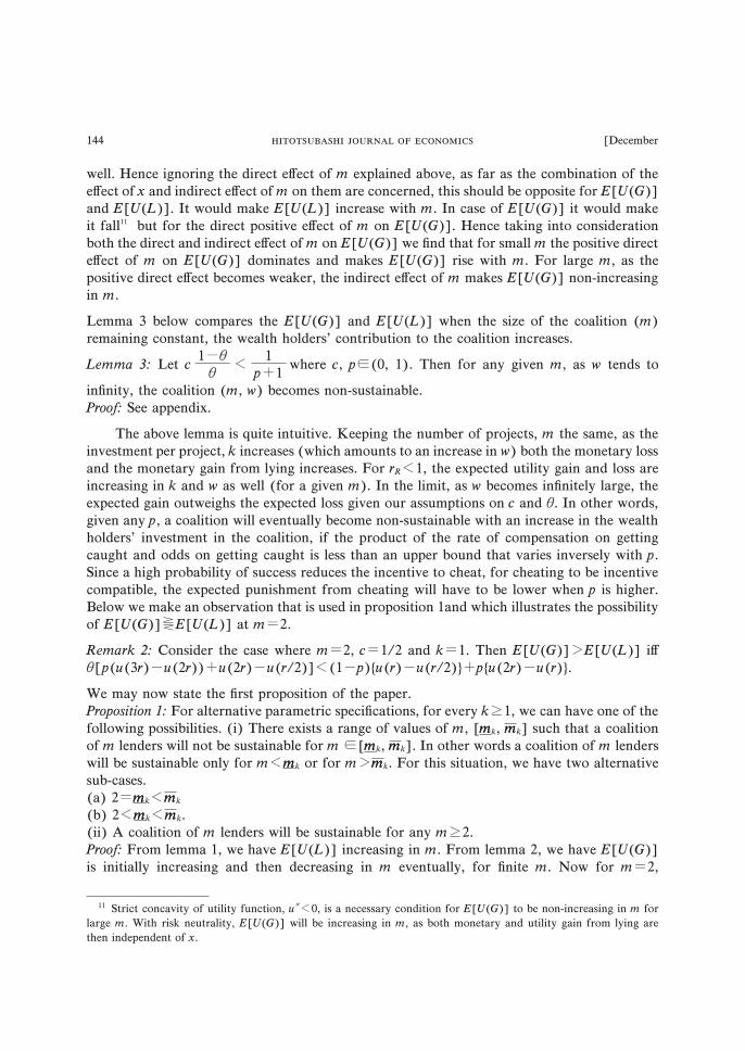
Lemma 3 below compares the E[U(G)] and E[U(L)] when the size of the coalition (m)
remaining constant, the wealth holders’ contribution to the coalition increases.
Lemma 3: Let c1�q
q� 1
p�1where c, p�(0, 1). Then for any given m, as w tends to
infinity, the coalition (m, w) becomes non-sustainable.
Proof: See appendix.
The above lemma is quite intuitive. Keeping the number of projects, m the same, as the
investment per project, k increases (which amounts to an increase in w) both the monetary loss
and the monetary gain from lying increases. For rR�1, the expected utility gain and loss are
increasing in k and w as well (for a given m). In the limit, as w becomes infinitely large, the
expected gain outweighs the expected loss given our assumptions on c and q. In other words,
given any p, a coalition will eventually become non-sustainable with an increase in the wealth
holders’ investment in the coalition, if the product of the rate of compensation on getting
caught and odds on getting caught is less than an upper bound that varies inversely with p.
Since a high probability of success reduces the incentive to cheat, for cheating to be incentive
compatible, the expected punishment from cheating will have to be lower when p is higher.
Below we make an observation that is used in proposition 1and which illustrates the possibility
of E[U(G)]�E[U(L)] at m�2.
Remark 2: Consider the case where m�2, c�1/2 and k�1. Then E[U(G)]�E[U(L)] i#q[p(u(3r)�u(2r))�u(2r)�u(r/2)]�(1�p){u(r)�u(r/2)}�p{u(2r)�u(r)}.
We may now state the first proposition of the paper.
Proposition 1: For alternative parametric specifications, for every k�1, we can have one of the
following possibilities. (i) There exists a range of values of m, [mmk, mmk] such that a coalition
of m lenders will not be sustainable for m�[mmk, mmk]. In other words a coalition of m lenders
will be sustainable only for m�mmk or for m�mmk. For this situation, we have two alternative
sub-cases.
(a) 2�mmk�mmk
(b) 2�mmk�mmk.
(ii) A coalition of m lenders will be sustainable for any m�2.
Proof: From lemma 1, we have E[U(L)] increasing in m. From lemma 2, we have E[U(G)]
is initially increasing and then decreasing in m eventually, for finite m. Now for m�2,
11 Strict concavity of utility function, u��0, is a necessary condition for E[U(G)] to be non-increasing in m for
large m. With risk neutrality, E[U(G)] will be increasing in m, as both monetary and utility gain from lying are
then independent of x.
=>IDIHJ76H=> ?DJGC6A D; :8DCDB>8H [December+..

E[U(G)]�E[U(L)] (according as a condition analogous to that stated in remark 2 holds or
does not hold). Therefore if at m�2, E[U(G)]�(�)E[U(L)], then E[U(G)] must cross
E[U(L)] curve once (twice). Hence, in either case mmk exists and mmk�2. This is the case stated
in (i)(a). Again if at m�2, E[U(G)]�E[U(G)], then (using lemmas 1 and 2) E[U(G)] will
cross E[U(L)] curve twice and in that case mmk exists and mmk�2. This is the case stated in (i)
(b). Alternatively the E[U(G)] curve will lie below E[U(L)] curve for all m, as stated in case
(ii).
Part (i)(a) of proposition 1 describes the situation where small coalitions (m�mmk) are
non-sustainable. So coalitions will be formed in equilibrium only if a large number of rich
wealth holders come together. The other sub-case which is the most illustrative of the
emergence of financial dualism tells us that coalitions of only small (m�mmk) and large (m�mmk) sizes may be observed. We discuss this possibility in greater detail throughout the rest of
the paper. Case (ii) refers to the situation where coalitions of all sizes are sustainable. Its
implications are discussed in subsection 2 of section V.
Corollary 1: (a) mmk is eventually increasing in k.
(b) As k��, mmk��.
(c) mmk is eventually decreasing in k.
Proof: Follows from lemma 3. Note that k�w/m.
Corollary 2: mmk and mmk is unique for every k.
Proof: Follows from lemmas 1 and 2.
IV . Emergence of the Formal and the Informal Sectors or Financial Dualism
1. Structure of Coalitions
The coalition space (m, w) illustrated in figure 1 consists of a set of discrete points along
each ray corresponding to m�2, 3, 4, .... . The curves marked as mmk and mmk based on
corollaries 1 and 2 delineate the space into the set of sustainable and non-sustainable
coalitions.12 As the latter will never be formed we will focus only on the coalitions that are
sustainable. Below we specify several subsets of the set of the sustainable coalitions S (which
are illustrated in figure 1).
A�{(m, w): w�wB and m�mm1 (�wB)}
A��{(m, w): wB�w�wC and m�mmk}
C�{(m, w): w�wC and m�mmk}
D�{(m, w): w�wC and m�mmk} where wB�kmmk and wC�kmmk for k�1 and the sets A, A�, C,
D are mutually exclusive and exhaustive with S�A�A��C�D.
In figure 1, the dark points belonging to the regions marked B(�A�A�), C and D
represent some of the elements of the set of sustainable coalitions. Since the coalitions in A and
those in A� do not di#er with respect to our later analysis, therefore we consider the union of
these two sets and call it B. As is obvious, the coalitions in C and D may be formed only by the
very rich, with wealth larger than wC. However, the coalitions in D are much larger than those
in C. Therefore, rich wealth holders can form a coalition in D only if there is su$ciently large
12 These curves cut each ray only once (corollary 2)
2007] :C9D<:CDJH ;DGB6I>DC D; ;>C6C8>6A 9J6A>HB +./

number of them. The coalitions in B, unlike C and D, may be formed by wealth holders with
wealth less than wC as well; these are also smaller in size compared to those in D. Thus smaller
coalitions may be formed either by large or small wealth holders. However, only the rich can
form the large coalitions in D. We now state certain lemmas.
Lemma 4: Individuals with W�wC will prefer forming coalitions (m, w)�D rather than C.
Proof: See appendix.
Lemma 4 states that forming larger coalitions is more desirable than forming smaller
coalitions. The result is intuitively clear as individuals are risk averse. Now suppose the initial
distribution of wealth is such that the number of individuals with wealth W�wC, is larger than
mm1 so as to allow the formation of a large coalition in D; but it is not large enough to allow the
formation of many large coalitions in D. In other words we consider a distribution such that:
Remark 3: Richer wealth holders form one single large coalition in D. The less wealthy, that
is individuals with wealth less than wC form small coalitions, in B.
2. Deposit Taking and the Formation of Bank
We denote the size of the coalitions corresponding to the di#erent zones indicated in
figure 1 by mi, i�B, C, D. Given that the rich form coalition in D, individuals with wealth less
than wC, face a third investment alternative; these individuals may now keep deposits with the
coalition in D, for a certain return rd, the gross interest on deposits.13 From now on, for ease
of exposition, we refer to the large coalition mentioned above, possibly deposit taking, as the
13 Note that the wealth holders forming coalitions in B will not keep deposits with coalitions formed by the rich
in C.
F><. 1
=>IDIHJ76H=> ?DJGC6A D; :8DCDB>8H [December+.0

“bank”.
Now given the option of keeping deposits with the bank, these wealth holders constituting
the smaller coalitions in B will ask for a risk premium from the entrepreneurs. Let z(�r) be
the rate of return (inclusive of risk premium) charged by the coalition (mB, w) from the
entrepreneurs. In the absence of deposit keeping, the rate of return on loans r(�aq) is
determined by Nash bargaining, between the entrepreneur and lender. Then z is defined by the
relation EmB
���
u����
xwz
mB
��
� ��u(wrd), given the rd chosen by the bank. Question is whether paying
z is feasible for the entrepreneur i.e. z�q? This is crucial since the wealth holders constituting
the smaller coalitions in B, will find keeping deposits with the bank attractive i# the answer is
no i.e. z�q. This is equivalent to the following condition:
EmB
���
u����
xwq
mB
��
� ��u(wrd) (1)
Thus we have,
Remark 4: Bank deposits are optimal for the smaller wealth holder i# the interest rate inclusive
of risk premium z is greater than q.
Question now arises as to how banks choose the risk free interest on deposits. For our analysis
we make the following assumption.
Assumption 2: rR is increasing in wealth.
z is increasing in rd. Further by assumption 2, z is increasing in w as well. Now as rd falls
the bank earns more per depositor. On the other hand, since z is increasing in both w and rd
therefore as rd falls, the critical level of w, above which wealth holders become depositors,
increases. Hence as rd falls, the number of depositors and the bank’s total deposits decrease. This
trade o# yields optimal value of rd�r�d at which the banks profit is maximum.
Remark 5: An optimal interest rate on deposits exists for the banks.
3. Possibility of Financial Dualism
We now check for the possibility of financial dualism. That is we check whether there will
always be some wealth holders who prefer keeping deposits with the large coalition in D
coexisting with other wealth holders who continue with local lending. For this, it is su$cient
to check the validity or otherwise of relation (1) for all w, given any rd. Again since z is
increasing in rd it is su$cient to check it for the highest possible value of rd�rrd�
EmD
���
u����
xr
mD
��
� ��pr�e�paq�e14; where the expected utility term is the maximum utility that
the bank can earn from return per unit of deposits. If local lending exists when return on
deposits is the highest then it will exist for lower returns on deposits as well.
Since we are interested in showing existence we need to show it for any one value of m.
Specifically we consider the case mB�2, which implies w�k2. Accordingly, we check whether,
for a given k,
14 Note that as mD��, rrd (mD) �pr. Hence rrd�pr�e, for large and finite m. This follows from the weak law
of large numbers.
2007] :C9D<:CDJH ;DGB6I>DC D; ;>C6C8>6A 9J6A>HB +.1

pu(2kq)�(1�p)u(kq)�u(2kpaq) (2)
For our analysis we consider the class of utility functions given below and focus on the case
A�0, (for which assumptions 1 and 2 hold):
u(v)�(A�v)b 0�b�1, A�0 and v�max[�A, 0]
For the above utility function (2) is equivalent to the following inequality
p(A�2kq)b�(1�p)(A�kq)b�(A�2pakq)b (3)
We now state lemma 5 which is based on inequality (3).
Lemma 5: For the class of utility functions stated above inequality in (3) is (a) satisfied for
large k (b) gets reversed for k�1.
Proof: See appendix.
Remark 6 below summarises the implications of the lemma.
Remark 6: (a) Moderate wealth holders (k reasonably large) will prefer keeping deposits with
bank rather than lending locally. (b)For small wealth holders (k small) there exists a value of
k (or at least one value of k) such that, the wealth holders with w�k2 will find it profitable
to engage in local lending and finance the home projects, rather than keeping deposits with the
bank. We christen these wealth holders as “informal lenders”.
The higher risk aversion of the relatively richer segment of wealth holders imply a larger
risk premium, which the entrepreneurs running the home project may not be able to pay. This
induces this middle segment to keep deposits with the bank. Thus at least for some wealth
holders belonging to the lowest end of the spectrum, the degree of risk aversion will not be
strong enough to make the risk premium infeasible for the local entrepreneurs. These wealth
holders will prefer funding the home project rather than keeping deposits with the bank
thereby establishing the basis for financial dualism. The above analysis is based on rd�rrd. The
argument may be extended and will hold more strongly for rd�rrd. Thus for the wealth holders
constituting small coalitions (partnerships), we get two cases. One segment of these wealth
holders, i.e. those belonging to the lowest part of the spectrum, will continue financing local
home projects as small cartels. These wealth holders will constitute the local informal lenders.
The other relatively richer segment (i.e. the middle segment of the spectrum) will keep
deposits with the large coalition formed by the richest segment of the wealth holders. These
wealth holders (the middle wealth segment) along with the richest will constitute the formal
credit market.
Proposition 2: We see the emergence of financial dualism with large wealthy coalitions acting
as deposit taking banks and smaller wealth holders either acting as local lenders or keeping
deposits with the bank.
4. Discussion
We start with a given distribution of wealth holders each with a home project. As wealth
holders do not have any information about other projects, unilateral diversification is not
feasible. We then consider the possibility of wealth holders diversifying their portfolios
through formation of coalitions by investing multilaterally and exchanging inside information
=>IDIHJ76H=> ?DJGC6A D; :8DCDB>8H [December+.2

about their respective home projects to avoid strategic default by entrepreneurs. This will work
only if truthful revelation of information by all wealth holders can be implemented as a
self-enforcing arrangement. We allow for such a possibility by incorporating payment of
compensation as a punishment for default (as court is the less attractive option).Our analysis
shows sustainable coalitions can be formed only when few wealth holders form small coalitions
or a large number of wealth holders form very large coalitions. As investment is indivisible,
large coalitions can be formed only by the very rich who have enough wealth to invest in all
the projects. However, sustainable small coalitions can be formed either by the rich or by the
poor.
If the number of rich wealth holders is small, then we see the existence of local lending
either by individuals or small coalitions as in a traditional society. These local bankers however
are not in a position to receive deposits. For example, the “country” banks of England or early
modern bankers in India. If the number of rich is large, who might be initially spread across
geographical regions, a large coalition in the nature of joint stock banking is born. The early
joint stock banks in England illustrate this natural development of the banking system when
not hampered by artificial barriers in the wake of Banking Copartnership Act 1826. Given that
such a large coalition exists with a large number of projects under its sponsorship and hence
with a well diversified investment base, other wealth holders who were previously forming
small coalitions will now have the option of taking advantage of risk diversification by keeping
deposits with the large coalition and earning a certain return. This latter option will not be
there if the rich were forming small coalitions
Given the broad investment base, banks can always o#er a return larger than r and still
make a profit. Further, given this opportunity of earning a fixed and certain return, the smaller
wealth holders who are members of small coalitions will ask for a return greater than r, as risk
premium. With risk aversion increasing in wealth, it is the relatively richer among this class of
small wealth holders who will ask for higher risk premia, which may be infeasible for the
entrepreneur. This class will therefore keep deposits with the bank. The lowest segment will
continue to lend locally as members of small coalitions resulting in a dualistic credit market.
In India, the emergence of modern banking can be traced to the establishment of Allahabad
Bank, the Alliance Bank of Simla and the Oudh Commercial bank during the second half of
the 19th century as joint stock banks with a system of receiving deposits regularly from the
public. While these joint stock banks emerged as the precursors of modern banking in India
some of the small indigenous bankers have continued to operate catering to the needs of mostly
small borrowers who are denied credit by the large banks.
The discussion so far primarily deals with the consequences of case (i) (b) of proposition
1. In the event that (i) (a) is realised, as the smaller coalitions are not sustainable, there is no
scope for risk diversification locally. So the chances of deposit keeping increase.15
15 The implication for case (ii) is ambiguous when rR�1 and increasing. Now smaller wealth holders forming
the smaller coalitions are likely to ask for higher risk premium because of less scope for diversification locally. But
at the same time their relative risk aversion is lower inducing them to ask for lower risk premium. Thus it is
di$cult to determine the extent of deposit keeping in this case.
2007] :C9D<:CDJH ;DGB6I>DC D; ;>C6C8>6A 9J6A>HB +.3

V. Robustness Considerations
We now explore the consequences of relaxing some of the assumptions considered earlier.
1. Coalitions with Di#erentiated Investments
We now raise the question whether wealth holders contributing di#erent amounts of
wealth can form sustainable coalitions. Here one can establish the following.
Proposition 3: A coalition among wealth holders who contribute widely di#erent amounts is not
sustainable. Hence rich will not collude with the significantly poor.
Proof: Let us consider a coalition with variable investments (m, ki) with k1�k and ki�k for
i�2, ...., m. The expected utility gain to wealth holder 1 from lying is E[U1(G)]�
qEm
���
u����
����
(m�x�1)k�Sm
2
hi
��
r���u(xkr)
���E[U(G)] (as in definition 1a). Also E[U1(G)]
is increasing in Sm
2
hi where hi�ki�k�0, i�2, ...., m. The expected utility loss is E[U1(L)]�
E[U(L)] (as in definition 1b). It follows that,
(a) if E[U(G)]�E[U(L)] then E[U1(G)]�E[U1(L)] and
(b) if E[U(G)]�E[U(L)] then E[U1(G)]�E[U1(L)] for some large value of Sm
2
hi
In other words, suppose a wealth holder investing k per project has the incentive to fink
when the remaining wealth holders invest identical amounts k. It follows that he has greater
incentive to fink if the investment per project for the remaining (m�1) wealth holders ki�k.
Thus if coalition (m, k) with equal contributions is non-sustainable then (m, ki) is also
non-sustainable. On the other hand if the coalition (m, k) is sustainable then (m, ki) will be
non-sustainable for large Sm
2
hi. As the utility function is assumed to be increasing throughout,
an initially sustainable coalition becomes unsustainable when the aggregate excess wealth of
the others, over the poorest wealth holder, crosses a certain limit.
Since the trigger is Sm
2
hi, the transition will take place whether one of the partners
contributes a very large additional amount or all (m�1) wealth holders contribute moderately
large additional amounts each. Moreover, the same transition will take place if instead of some
partners’ wealth increasing, some peoples’ wealth decrease. Hence, if the variation among the
contributions is too large, then a sustainable coalition can not be formed. Thus, any rich
wealth holder, when faced with a choice of partners in a coalition, will calculate the aggregate
excess wealth. If a potential partner has a much lower contribution to make, then this
aggregate will cross the threshold. Hence, this rich wealth holder will desist from forming such
a coalition. This concludes the proof of proposition 3.
Proposition 3 implies that even if we allow for coalition among wealth holders contribut-
ing di#erent amounts, this variation can not be very large for sustainability. Hence apart from
the di#erence that the set of sustainable coalitions will now include some partnerships with
moderately unequal contributions, allowing for variable investments does not qualitatively
alter the rest of our analysis
=>IDIHJ76H=> ?DJGC6A D; :8DCDB>8H [December+/*

2. Relaxing the Risk Aversion Assumptions
Empirical studies of risk aversion (Chou et. al., 1992, Barsky et. al., 1997, Heinemann,
2003, Meyer and Meyer, 2004) reveal that estimates of rR parameter can have any value both
larger and smaller than one, including negative values which implies that agents are risk
loving. These estimates are only average values. Thus actually there exists a distribution of
values for the rR parameter over the population of agents. Our model shows that if we consider
a population of heterogeneous agents with di#ering rR, then financial dualism is possible as long
as there exists a subset of the population with value of rR�1. The richer among these would
form banks while those with lower wealth would keep deposits with bank or lend locally. The
wealth holders for whom rR�1 may or may not form large coalitions. In latter case wealth
holders would finance local projects as in traditional financial system.
Secondly, in this model an increase in the degree of risk aversion causes both expected
utility gain and loss from lying to decrease, all other parameters held constant. This allows for
the possibility of a sustainable coalition becoming non-sustainable (if the decrease in E[U(G)]
is less than the decrease in E[U(L)]), which reduces risk diversification. Thus increase in risk
aversion need not necessarily lead to increase in risk diversification in an environment with
asymmetric information and strategic default. This is contrary to the standard literature,
which predicts a direct relationship between the two.
Finally, we consider the implications of relaxing assumption A.2. With risk aversion
decreasing in wealth, the behaviour of the middle and lowest segment of the wealth holders are
reversed. Now, the higher risk aversion of the lowest segment implies that this segment
becomes depositors as the higher risk premium may be infeasible. The relatively richer segment
of wealth holders outside the coalition (the middle segment), on the other hand, would ask for
a lower risk premium and lend locally, i.e. operate as informal lenders.
3. Endogenous Determination of Compensation for Sustainable Coalition
In our model c is exogenously given. Question may arise as to whether c can be
endogenously determined so as to make any coalition sustainable i.e. given any (m, k) does
there always exist a value of c�[0, 1] that will make (m, k) sustainable. We consider the
extreme case in which c�1. In this case, expected utility from returns on investment if an
wealth holder tells the truth is Em[u(xkr)]. The expected utility if he lies is
qEm[u((m�x�1)kr)] as with c�1 the wealth holder retains nothing if he lies and gets
caught. Comparing the expected utilities we find that for su$ciently large q(close to 1) the
expected utility from lying may be greater than the expected utility from telling truth, given
any (m, k). This means the coalition (m, k) would be non-sustainable even for c�1, which
implies it is non-sustainable for all c�1. Thus making c endogenous does not rule out the
possibility of non-sustainable coalitions.
4. Relaxing the Assumption of Binomial Distribution
This paper is based on the assumption of independent and identical projects. Giving up
independence is not interesting as it reduces the scope for risk diversification. Relaxing the
assumption of identical projects, allows for di#ering output and probability of success across
2007] :C9D<:CDJH ;DGB6I>DC D; ;>C6C8>6A 9J6A>HB +/+
projects leading to di#erent combinations of risk and return. This problem can be analysed
only in a simplified framework, as it is analytically intractable in a general model as ours.
While other probability distributions (eg.,Poisson and discrete version of Beta) that lend itself
to similar analysis exist (Marshall and Olkin; 1979) these distributions do not arise from
stochastic processes that match with the nature of projects considered.
VI . Conclusion
Starting with a given initial distribution of wealth holders (who are potential lenders) we
show the emergence of the formal sector consisting of joint stock banks and informal sector
consisting of indigenous bankers. This is done in terms of a model of the credit market where
each lender has inside information about a project’s returns i.e. whether it succeeded or failed.
These projects are carried out by entrepreneurs who otherwise play a passive role. Risk
spreading suggests lenders should invest in each other’s home projects. The trouble is a lender
could lie about whether his home project succeeded or not and he can be caught only with
some probability. Contract enforcement is imperfect. Three types of financial arrangements
are considered. A lender can just invest in his home project. Lenders can form a coalition and
members can punish other members if they are caught lying by imposing a fine. An
incentive-compatibility constraint is derived which shows the coalition sizes for which, a
member will not cheat. Finally, a lender can deposit money in one of the coalitions formed by
others.
Using the above model, we show for certain parametric configurations, the possible
existence of a large sustainable coalition of wealth holders emerging as the joint stock bank
along with informal lending by smaller coalitions. If a coalition is quite large then wealth
holders from the middle wealth class find it profitable to invest their money with the coalition
for a certain return. The coalition also benefits from this. Thus, we have deposit taking joint
stock banks owned by large number of big shareholders as large coalitions can be formed only
by the very wealthy. The small wealth holders however find it profitable to form small
coalitions giving birth to local cartels, of the type found in the informal sector. This segment
of wealth holders will continue financing local projects (as local moneylenders and indigenous
partnership banks) rather than keeping their wealth as deposits with the large coalition or
bank.
In other words, we highlight the endogenous creation of financial dualism. While dynamic
models of repeated interaction and static models using exogenously given penalty function
have been used in the literature for analyzing stable coalition formation in a wide range of
contexts such as rural cooperation, mutual insurance, foreign direct investment, self-enforcing
wage contracts, this paper models a process of coalition formation for explaining the source of
financial dualism. The latter being an important feature of the credit markets of less developed
countries, plays an important role in the design of credit policy for curbing the presence of the
informal lenders.
Our model of financial dualism captures the experience of the developed countries in
Europe, especially U.K. and Germany, during their early days of development and also the
experience of the developing countries like India. As these country experiences suggest, the
history of modern banking can be traced to the formation of the joint stock banks, which stand
=>IDIHJ76H=> ?DJGC6A D; :8DCDB>8H [December+/,

in contrast to the native bankers. Typically the joint stock banks are initially formed by the
local rich and attract deposits. The depositors belong to the middle wealth segment. The
indigenous bankers consisting of the small wealth holders are hardly ever in a position to
receive deposits. This is the formation of financial dualism that we model in this paper. We
finally discuss the robustness of our conclusions with respect to certain structural assumptions.
In particular we show that coalitions with widely di#erent contributions are not sustainable.
Consequences of alternative assumptions on risk aversion are also discussed.
AEE:C9>M
In lemmas 1 to 2, as the constant “k” operates only as a scale factor, for the sake of
notational simplicity we omit k in the utility expressions.
Proof of Lemma 1:
Nowd
dx[u(xr)�u((1�c)xr)� 1
x{u�(xr)xr�u�((1�c)xr)(1�c)xr}�0 i# u�(z)z is increas-
ing in z. This requires that u�(z)�u�(z)z�0 �� zu�(z)
u�(z)�1. Hence for rR�1, [u(xr)�
u((1�c)xr)] is strictly increasing in x. Further, as x�B(m, p), therefore using theorem 3.J.2
in Marshall and Olkin (1979) it follows that Em[u(xr)�u((1�c)xr)] is strictly increasing in
m. For functions of scalars, increasingness is equivalent to schur-convexity (refer to Marshall
and Olkin (1979), definition 3.A.1.). So the theorem is applicable in the present context. Hence
result follows.
In order to prove Lemma 2, we need certain results, which are demonstrated in Lemma
A.1 to Lemma A.3 below. But first we observe that using definition 1a and the Mean Value
Theorem expected utility gain may be expressed as E[U(G)]�Em[(m�1)kr u�(x(x, m))]
where xkr�x�(m�x�1)kr. Hence denoting Em[u�(x(x, m))] by y(m) we have E[U(G)]�(m�1)kry(m).
Lemma A.1: u�(x(x, m)) is strictly decreasing in x.
Proof: By Mean Value Theorem it follows that
u((m�x�1)r)�u(xr)�(m�1)r u�(x(x, m))
u((m�x)r)�u((x�1)r)�(m�1)r u�(x(x�1, m))
By concavity of the function u we have,
u((m�x�1)r)�u(xr)�u((m�x)r)�u((x�1)r)
� u�(x(x, m))�u�(x(x�1, m))
Given the above inequality, again by concavity of the function u w.r.t. the variable x we
have, x(x, m)�x(x�1, m). Therefore x is increasing in x.
This implies that u�(x(x, m)) is decreasing in x i.e. u(x(x, m)) is concave in x.
Lemma A.2: u�(x(x, m))is decreasing in m.
Proof: By Mean Value Theorem we have,
2007] :C9D<:CDJH ;DGB6I>DC D; ;>C6C8>6A 9J6A>HB +/-

u((m�x�1)r)�u(xr)�(m�1)r u�(x(x, m))
� u((m�x�1)r)�u(xr)
(m�1)r�u�(x(x, m))
Similarly,u((m�x)r)�u(xr)
mr�u�(x(x, m�1))
By concavity of the function u we have,
u((m�x�1)r)�u(xr)
(m�1)r� u((m�x)r)�(xr)
mr
� u�(x(x, m))�u�(x(x, m�1))
Given the above inequality, again by concavity of the function u w.r.t. the variable x we
have, x(x, m)�x(x, m�1). Hence x is increasing in m.
This implies that u�(x(x, m)) is decreasing in m i.e. u(x(x, m)) is concave in m.
Lemma A.3: y(m) is decreasing in m.
Proof: From lemma A.1, u�(x(x, m)) is strictly decreasing in x. Further from lemma A.2,
u�(x(x, m)) is also decreasing in m. Hence y(m) is strictly decreasing in m. This is because for
functions of scalars decreasingness is equivalent to schur-concavity (see definition 3.A.1. in
Marshall and Olkin, 1979). Hence theorem 3.J.2. of Marshall and Olkin (1979) will still
remain applicable and hold even more strongly for u�(x(x, m))decreasing in m. Details of this
demonstration are routine but tedious and we omit them here.
Proof of Lemma 2:
Di#erentiating16 E[U(G)]�(m�1)ry(m), with respect to m, yields
dE[U(G)]
dm�(m�1)ry�(m)�ry(m)
Now, for m�2,dE[U(G)]
dm�r{y�(m)�y(m)}
�r{Em[u�(.)]�o(pm�1)�Em[u�(.)]}
�r{Em[u�(.)�u�(.)]�o(pm�1)}
This is analogous to the change in order of integration and di#erentiation as in the Leibnitz
rule. Further, as the magnitude of the term o(pm�1) will be of very small order compared to
the other two terms, the sign of the derivative will be the same as that of [u�(.)�u�(.)].
Now rR�1 by assumption, i.e. � zu�(z)
u�(z)�1. x�1, m�2 and r�1. Now take z�x, corre-
sponding to E[U(G)] as discussed above. Then z belongs to the interval (xr, (m�x�1)r) and
so z�1). Hence � zu�(z)
u�(z)�1 � u�(z)�u�(z)�0. Therefore for m�2,
dE[U(G)]
dm�0.
16 Here we use the di#erential notation, for expositional simplicity. The actual derivation in terms of successive
di#erences would only complicate the algebra and not add qualitatively to our findings.
=>IDIHJ76H=> ?DJGC6A D; :8DCDB>8H [December+/.

AgaindE[U(G)]
dm�0 i# � y�(m)
y(m)� 1
m�1. As m��,
1
m�1�0. For strictly concave
u(.) i.e. u��0,y�(m)
y(m)is negative (by Lemma A.3) making the LHS, � y�(m)
y(m)positive and
strictly bounded away from zero. Hence the above inequality does not hold, that is, E[U(G)]
is non-increasing in m for large m, when rR�0 and u��0. Thus lemma 2 holds for strictly
concave u(.). Note that, this result will continue to hold for a general k�1.
Proof of Lemma 3:
(E[U(G)]
(w�S
m
x�1
qP(x, m)(
(w
���
u����
(m�x�1)wr
m
���u
����
xwr
m
��
��
�Sm
x�1
qP(x, m)���
u�����
(m�x�1)wr
m
��
(m�x�1)r
m�u�
����
xwr
m
��
xr
m
���0
and(E[U(L)]
(w�S
m
x�1
(1�q)P�(x, m)���
u�����
xwr
m
��
xr
m�u�
����
(1�c)xwr
m
��
(1�c)xr
m
���0
since� zu�(z)
u�(z)�1 by assumption. Thus both E[U(G)] and E[U(L)] are increasing in w, for
a given m.
Now let u�(z)�e�0 (e is an arbitrary small number) as z��. Then as w��,(E[U(G)]
(w�
Sm
x�1
qP(x, m)e(m�1)r
m
q(m�1)r
m(since S
m
x�1
P(x, m)�1)
and(E[U(L)]
(w� S
m
x�1
(1�q) P(x, m)ecxr
m
� (1�q)ecr
m Sm
x�1
P(x, m)x
� (1�q)ecr
m Sm�1
x�1�0
m�1 Cx�1 px�1(1�p)m�x{(x�1)�1}
� (1�q)ecr
m[(m�1)p�1]
Comparing slopes as w��,(E[U(G)]
(w� (E[U(L)]
(waccording as
(m�1)
(m�1)p�1�
(1�q)
qc. Now at m�2,
(m�1)
(m�1)p�1� 1
p�1�1 and as m��, it tends to
1
p�1. Thus
(m�1)
(m�1)p�1is increasing in m. Therefore to ensure that
(E[U(G)]
(w� (E[U(L)]
(was w�
�, it su$ces to assume that c1�q
q� 1
p�1.
Proof of Lemma 4:
The expected utility from the return on money invested in a coalition by an individual wealth
2007] :C9D<:CDJH ;DGB6I>DC D; ;>C6C8>6A 9J6A>HB +//

holder is Em[u(xkr)], where k�w/m. Now Em[xkr]�wrp which is constant as m increases.
Further Var[xkr]�(wr)2 p(1�p)
m, which is decreasing in m. Hence for any given w,
Em[u(xkr)] is increasing in m (as wealth holders are risk averse).17
Proof of lemma 5:
(a) Multiplying through inequality (2) by (1/k)b, yields,
p����
A
k�2q
����
b
�(1�p)����
A
k�q
����
b
�����
A
k�2pakq
����
b
As k��, A/k�0. Using this and simplifying, the above inequality may be expressed as,
2b{(pa)b�p}�1�p. Expressing p as (1�e) and a as (1�h) , where e and h are arbitrarily
small positive numbers, we may substitute (1�e�h) for pa , since eh�0.The inequality may
now be expressed as, 2b{(1�e�h)b�1�e}�e. Considering the first two terms only in the
Binomial Expansion of {1�e�h}b i.e. {1�b(e�h)}, and ignoring the remaining terms as (e�h) and b, are both small numbers, we have,
2b{e�b(e�h)}�e
As 2b�1, the above inequality will hold if b(e�h) is very small. This requires that the
probability of success p and the wealth holder’s share in home project’s output a be high
(implying that the wealth holder enjoys a strong bargaining position). Moreover this requires
that the degree of relative risk aversion be high. This is expected for large k since relative risk
aversion is increasing in wealth by assumption. Thus for large k, z�q. As entrepreneurs can
pay at most q, therefore, the wealth holders will keep deposits with the bank.
(b) Multiplying through inequality (3) by (1/A)b yields,
p����
1� 2q
A
����
b
�(1�p)����
1� q
A
����
b
�����
1� 2paq
A
����
b
For large A, 2q/A is small. In that case considering the first two terms of the Binomial
expansion of����
1� 2q
A
����
b
su$ces, since the remaining terms in the expansion will be of very
small magnitude. Hence putting����
1� 2q
A
����
b
�1� 2qb
A, the above inequality, after simplific-
ation, may be expressed as, 2p�(1�p)�2pa. Since a�1, this inequality does not hold.
Hence, for k�1, the inequality in (3) gets reversed to “�”.
17 For related concepts see Huang and Litzenberger (1988).
=>IDIHJ76H=> ?DJGC6A D; :8DCDB>8H [December+/0

R:;:G:C8:H
Barsky, Robert B., F. Thomas Juster, Miles S. Kimball and Matthew D. Shapiro (1997),
“Preference Parameters and Behavioural Heterogeneity: An Experimental Approach in
the Health and Retirement Study”, mimeo, Survey Research Center and Department of
Economics, University of Michigan.
Basu, K. (1998), Analytical Development Economics: The Less Developed Economy Revisited,
Oxford University Press.
Basu, K. (1990), Agrarian Structure and Economic Underdevelopment, Harwood Press, Chur.
Bhaduri, A. (1977), On the Formation of Usurious Interest Rates in Backward Agriculture,
Cambridge Journal of Economics, 1, pp.341-352.
Bhattacharya, D. (1989), A Concise History of Indian Economy, 3rd Edition, Prentice-Hall of
India Pvt. Ltd.
Besley, T. and S. Coate (1995), “Group Lending, Repayment Incentives and Social Collat-
eral”, Journal of Development Economics, 46, pp.1-18.
Chou, R., R. F. Engle and A. Kane (1992), “Measuring Risk Aversion from Excess Returns
on a Stock Index”, Journal of Econometrics, 52, pp.201-24.
Coate, S. and M. Ravallion (1993), “Reciprocity without Commitment”, Journal of Develop-
ment Economics, 40, pp.1-24.
Deane, P. (1979), The First Industrial Revolution, 2nd Edition, Cambridge University Press.
Dutta, B., D. Ray and K. Sengupta (1989), “Contracts with Eviction in Infinitely Repeated
Principal-Agent Relationships”, in Bardhan, Pranab, ed. The Economic Theory of Agrar-
ian Institutions, Oxford University Press
Genicot, G and D. Ray (2003), “Group Formation in Risk Sharing Arrangements”, Review of
Economic Studies, 70, pp.87-113.
Heinemann, Frank (2003), “Risk Aversion and Incentive E#ects: Comment”, mimeo, Univer-
sitat Munchen.
Huang, C. and R.H. Litzenberger (1988), Foundations for Financial Economics, Elsevier
Science, North-Holland, N.Y.
Jain, S., (1999), “Symbiosis vs. Crowding Out: the Interaction of Formal and Informal Credit
Markets in Developing Countries”, Journal of Development Economics, 59, pp.419-444.
Johnson, H.J. (2000), Banking Alliances, World Scientific Publishers, Singapore.
Kaushal, G. (1979), Economic History of India: 1757-1966, Kalyan Publishers.
Kindleberger, C.P. (1984), A Financial History of Western Europe, London: George Allen and
Unwin Ltd.
Kocherlakota, N.R. (1996), “Implications of E$cient Risk Sharing without Commitment”,
Review of Economic Studies, 63, pp.595-610.
Ligon, E., J.P. Thomas and T. Worrall (2002), “Informal Insurance Arrangements with
Limited Commitment: Theory and Evidence from Village Economies”, Review of Eco-
nomic Studies, 69, pp.209-244.
Marshall, A.W. and Olkin, I. (1979), Inequalities: Theory of Majorization and its Applications,
Academic Press.
Meyer, Donald J. and Jack Meyer (2004), “Relative Risk Aversion: What do We Know?,”
mimeo, Western Michigan University.
2007] :C9D<:CDJH ;DGB6I>DC D; ;>C6C8>6A 9J6A>HB +/1

Mookherjee, D. and D. Ray (2001), Readings in the Theory of Economic Development, Edited
volume, Blackwell Publishers.
Ramakrishnan, R. T. S. and Thakor, A.V. (1984), “Information, Reliability and a Theory of
Financial Intermediation”, Review of Economic Studies, LI, pp.415-432.
Thomas, J. and T. Worrall (1988), “Self-Enforcing Wage Contracts”, Review of Economic
Studies, 55, pp.541-554.
Tun Wai, U. (1956), “Interest Rates in the Organised Money Markets of Underdeveloped
Countries”, IMF Sta# Papers, pp.258-62.
Tun Wai, U. (1957), “Interest Rates outside the Organised Money Markets”, IMF Sta#Papers.
=>IDIHJ76H=> ?DJGC6A D; :8DCDB>8H+/2