econstorMake Your Publications Visible.

A Service of

zbwLeibniz-InformationszentrumWirtschaftLeibniz Information Centrefor Economics

Wolf, Nikolaus; Ritschl, Albrecht

Working Paper

Endogeneity of Currency Areas and Trade Blocs:Evidence from the Inter-War Period

Papers / Humboldt-Universität Berlin, Center for Applied Statistics and Economics (CASE),No. 2004,10

Provided in Cooperation with:CASE - Center for Applied Statistics and Economics, HumboldtUniversity Berlin

Suggested Citation: Wolf, Nikolaus; Ritschl, Albrecht (2003) : Endogeneity of Currency Areasand Trade Blocs: Evidence from the Inter-War Period, Papers / Humboldt-Universität Berlin,Center for Applied Statistics and Economics (CASE), No. 2004,10

This Version is available at:http://hdl.handle.net/10419/22184

Standard-Nutzungsbedingungen:

Die Dokumente auf EconStor dürfen zu eigenen wissenschaftlichenZwecken und zum Privatgebrauch gespeichert und kopiert werden.

Sie dürfen die Dokumente nicht für öffentliche oder kommerzielleZwecke vervielfältigen, öffentlich ausstellen, öffentlich zugänglichmachen, vertreiben oder anderweitig nutzen.

Sofern die Verfasser die Dokumente unter Open-Content-Lizenzen(insbesondere CC-Lizenzen) zur Verfügung gestellt haben sollten,gelten abweichend von diesen Nutzungsbedingungen die in der dortgenannten Lizenz gewährten Nutzungsrechte.

Terms of use:

Documents in EconStor may be saved and copied for yourpersonal and scholarly purposes.

You are not to copy documents for public or commercialpurposes, to exhibit the documents publicly, to make thempublicly available on the internet, or to distribute or otherwiseuse the documents in public.

If the documents have been made available under an OpenContent Licence (especially Creative Commons Licences), youmay exercise further usage rights as specified in the indicatedlicence.

www.econstor.eu

Endogeneity of Currency Areas and Trade Blocs:

Evidence from the Inter-War Period

Albrecht Ritschl*

Nikolaus Wolf+

First draft: August 2002

This version: September 29, 2003

Abstract

Empirical research on the gravity model of international trade in the wake of Rose (2000) affirms that currency union formation doubles or triples trade. However, currency unions could also be established precisely because trade among their members was already high. In OLS estimation, this would cause endogeneity bias. The present paper employs both fixed effects and binary choice methods to trace endogeneity in the formation of historical currency arrangements. Studying the formation of currency blocs in the 1930s, we find strong evidence of endogeneity. We work with country group fixed effects and find that already in the 1920s, trade within the later currency blocs was up to three times higher than on average. The formal establishment of these blocs had only insignificant or even negative ef-fects on the coefficients. We also employ a probit approach to predict membership in these later ar-rangements on the basis of data from the 1920s. Results are remarkably robust and again indicate strong self-selection bias. Evaluated against the control groups, treatment effects in the 1930s were mostly absent. Even the post-war currency arrangements are visible in the inter-war data. In line with the theory of optimum currency areas, our results caution against optimism about trade creation by currency unions.

Keywords: Currency blocs, gravity model, endogeneity, treatment effects

JEL Classification Code: F33, F15, N70

* Dept. of Economics and CASE, Humboldt University Berlin; and CEPR. <ritschl@wiwi.hu-berlin.de>. + London School of Economics, <n.wolf@lse.ac.uk>. We are grateful to Alberto Alesina, Marc Flandreau, Volker Nitsch, Andrew Rose, Torsten Persson, Harald

Uhlig, and conference and seminar participants in various places for helpful comments on earlier versions. Thanks also go to Kristina Strunz and Charlotte Moeser for excellent research assistance.

2

I. Introduction

What is the effect of currency unions on international trade? Recent empirical research by

Rose (2000; 2001) finds that trade within currency unions is two to three times larger than a

gravity model of international trade would predict. The gravity model, now a standard tool of

the trade literature (see e.g. Anderson (1979), Deardorff (1998), Anderson and van Wincoop

(2003)), establishes that other things equal, trade between any two countries mainly depends

on distance and relative size. Within this model, the measured effect of currency unions on

trade is usually large.

But there is also a competing view. It is motivated by the theory of optimal currency areas

(OCA), as introduced by Mundell (1961) and McKinnon (1963) and further developed by

Frankel and Rose (1997; Frankel and Rose (1998), Dixit (2000), and Alesina and Barro

(2002). OCA theory argues that trade integration may give rise to monetary integration, as the

degree of economic integration between two countries affects the possible welfare gains of a

monetary union. This may cause endogeneity bias: national currencies may have been aban-

doned and a currency union formed precisely because trade was already high.

Assessment of this issue is a typical problem in the analysis of treatment effects (on the key

issues, see Heckman et al. (1999). The analyst aims to find out about the effects of exposing

an observation unit to a treatment, be it a drug, a training program, or a currency arrangement.

Evaluating the effects of any treatment necessarily involves an unobservable counterfactual,

namely, the state of the treated observation unit had there been no treatment. There are two

principal ways to overcome this problem, either by making the comparison with the individ-

ual’s state before the beginning (or after the end) of the treatment, or by comparison with a

control group of other observation units not under treatment. The present paper looks into a,

possibly unique, historical case where both, the intertemporal and the cross-sectional ap-

proaches to identification can be applied without contamination.

The literature on currency arrangements has just begun to pay attention to the proper identifi-

cation of treatment effects. While initial work of Rose (2000) consisted in cross-section analy-

sis, recent work has fanned out along both the intertemporal and the cross-section dimension.

To use information over the cross section and over time simultaneously, it has become com-

mon to apply panel data techniques, see e.g. Glick and Rose (2002) and Rose (2001) for post-

war data and Flandreau and Maurel (2001) or López-Córdova and Meissner (2003) for data

3

from the classical gold standard. Recent work of Estevadeordal, Frantz and Taylor (2003)

provides a survey of existing applications with historical data. The key finding of Rose,

namely that the creation of a currency union has very large trade creating effects, usually sur-

vives in these specifications. To improve on the proper choice of a control group, Persson

(2001) has proposed a two-stage procedure to the gravity equation, akin to Heckman’s Heckit

estimator. In a first stage, a binary choice approach is employed to select a suitable control

group from common characteristics. In a second stage, the gravity equation measuring the

treatment effect is run for a subsample including the both treated and the control group. Re-

stricting comparison to this pre-selected control group, Persson (2001) finds the treatment ef-

fects of currency unions to become significantly smaller.

Identification of the treatment effects of a currency arrangement along the intertemporal di-

mension faces the problem of anticipation effects: trade among the future members of a cur-

rency arrangement may rise in the expectation that a formal arrangement will be established

in the future. In many cases, it is very difficult – if not impossible – to disentangle such re-

verse causation and endogeneity, since both would predict greater levels of trade before the

actual formation of a currency union. One of the key contributions of this paper is to examine

a historical episode in which new currency areas formed in the aftermath of a cataclysmic,

unexpected event. This allows us to discount anticipation effects, and interpret our results as

evidence in favor of endogeneity.

The cataclysmic event to which we refer is the Great Depression and the subsequent collapse

of the gold standard. In the aftermath of the Great Depression, the gold standard was replaced

by several regional currency blocs. If the formation of these regional currency blocs was un-

expected, anticipation effects are likely to be absent from the data. Then, information on trade

relations before the Great Depression could serve to identify the effects of the post-depression

currency arrangements.

There exists a solid body of literature which argues that the Great Depression was indeed an

unexpected event. Hamilton (1987; 1992) has argued that deflation after 1929 came unexpect-

edly. Dominguez, Fair and Shapiro (1988) examined the performance of contemporary busi-

ness-cycle forecasts through leading indicators, including a series by Irving Fisher, and found

that they fail to predict the recession. Ritschl and Woitek (2001) find that predicting the de-

pression from monetary variables is equally difficult. All these results imply that the gold

4

standard was still credible before 1929 and that anticipation of future currency blocs did not

influence agents’ behavior.

Eichengreen and Irwin (1995) estimate three separate cross-sectional gravity models for the

benchmark years of 1928, 1935, and 1938. They actually do find effects of the later currency

blocs in their regression for 1928, however without having a clear interpretation for this re-

sult. In parts of our paper we build on their results; however we pool our cross-section trade

data over the benchmark years. We estimate an augmented version of the gravity model as in

Glick and Rose (2002) and Estevadeordal, Frantz and Taylor (2003). This model can be

viewed as a reduced form of different models of trade with solid microfoundations, see

Anderson and van Wincoop (2003), Redding and Venables (2001), Eaton and Kortum (2002).

Essentially, we regress bilateral trade volumes between countries on a vector of controls,

given by the gravity model, and a set of dummy variables, designed to capture the impact of

currency arrangements between the countries.

One key contribution of our paper is to analyze the famous currency dummies a little closer.

First, in most of our paper we drop the assumption of Glick and Rose (2002) who chose to

pool all members of any currency union in their sample into one dummy variable, thus re-

stricting all currency unions to have the same average effect. We will rather adhere to the ap-

proach of Eichengreen and Irwin (1995) and measure the trade effect of each currency ar-

rangement separately. Nitsch (2002) has shown that doing so in Rose (2000)’s post-war data-

set, trade creation effects vary substantially. We will find similar effects. Second, we examine

the behavior of these dummies over time in order to identify the treatment effect of currency

arrangements intertemporally. For each currency area, we define two dummy variables. One is

our analog to Andrew Rose’s (2000) CU variable. It is equal to one while the formal currency

arrangement is operative. The second includes the same country group; however, it is equal to

one for the whole sampling period. Essentially, this second dummy is a country group fixed

effect. It captures any trade that is higher already before a currency bloc is formed (or after it

has dissolved).

Introducing country group dummies instead of country pair fixed effects for the trade among

members of a currency arrangement has two advantages. First, it allows direct comparison of

the group of countries under a currency arrangement with the same reference group before

treatment. Second, inclusion of country group dummies increases degrees of freedom and re-

5

duces potential collinearity problems. Including a full set of country-pair fixed effects in a

panel estimation might be desirable on theoretical grounds, see e.g. Anderson and van Win-

coop (2003). However, there is a deeper identification issue here: as country-pair fixed effects

on every trade pair pick up any other time-invariant pair characteristics (such as distance, lan-

guage, colonial ties, etc.), they make the estimation of a gravity model of trade essentially in-

feasible.1 Choosing country group instead of country pair fixed effects is a way to circumvent

this problem.

Estimating the gravity model in the presence of appropriate fixed effects, in this paper we ob-

tain strong evidence in favor of endogeneity. Most of the major currency and trade blocs that

formed in the 1930s are visible already in the data from the 1920s. The coefficients on the

country group dummies indicate that already prior to the Great Depression, trade among the

members of the later blocs was 2-3 times larger than predicted by the gravity model. Those

are precisely the orders of magnitude obtained by Rose and his coauthors. We find that con-

trolling for this endogeneity, the effects of actually establishing these currency arrangements

in the 1930s are most often insignificant or even negative.

A deep identification issue presents itself also in the cross-sectional dimension. Labor econo-

mists have pointed to the need for the evaluation of policy treatment effects against properly

chosen control groups, see Heckman et al. (1999) for a survey. All estimation methods can be

seen as a way of identifying the treatment effect on the treated against a counterfactual, the

state of the treated in the absence of treatment. As this counterfactual is inherently unobserv-

able, identifying assumptions need to be made to infer the counterfactual from observations

on something else. This can be either the group of the treated at different points in time, as-

suming other characteristics of this group to be constant over time. This is the rationale be-

hind fixed effect estimation, which assumes the group of the treated to be its own control

group.

Alternatively, a counterfactual can be constructed by suitable cross-sectional comparison. In

the cross-section domain, econometric comparison of the treated group with the control group

is prone to be contaminated by two effects. First, the treatment itself may have indirect effects

on the control group. In the context of trade and currency areas, these indirect effects may

1 This point is also made by Estevadeordal et al. (2003).

6

consist in trade diversion away from third parties. In the empirical literature on currency ar-

eas, the only paper we are aware of that controls for trade diversion is Eichengreen and Irwin

(1995), which finds strong such effects during the inter-war period. To the extent that indirect

effects are not fully controlled for, measurement of the treatment effect may be biased. Sec-

ond, the group of the treated may itself not have been randomly selected, leading to endogene-

ity bias. Fixed effect estimation is only an incomplete way to circumvent this problem, as it

critically depends on the time invariance over the panel of any factors causing endogeneity.

To tackle this issue, we follow Persson’s (2001) binary choice approach to control group se-

lection. The idea here is to find a probability, called the propensity score, that a given observa-

tion is being selected into the treatment group (the currency arrangement), given a vector of

fundamental characteristics. Persson employs this approach to construct a control group for

the gravity equation. In this paper we use levels of trade integration as estimated by a gravity

model to directly predict the formation of currency blocs in a binary choice model. From

Alesina and Barro (2002) we borrow the concept of core country in international trade. We

view the trade blocs emerging in the 1930s as hegemonic rivalry, and predict membership

from trade with the respective core country. To exclude indirect effects, we restrict ourselves

to trade data from the 1920s, prior to the establishment of currency areas in the 1930s. Again,

results confirm that the formation of the currency unions of the 1930s was endogenous: all the

major fault lines are visible already in the 1920s; the binary choice model predicts bloc forma-

tion quite well.

Endogeneity may be put to an even harder test. If path dependence of the various trade and

currency arrangements was prevalent in the inter-war period, it is natural to ask if post-war

European integration was foreshadowed in the inter-war data. It was indeed. Both the gravity

equation and the binary probit approach provide evidence of intense trade among the future

members of the postwar European blocs.

The remainder of this paper is structured as follows. Section II introduces the model setup and

also discusses data sources and methods. Section III provides a brief review of the historical

background. Section IV presents benchmark estimates for the gravity model and shows the

effects of endogeneity on the results. Section V carries out a number of robustness checks and

explores alternative specifications of the gravity equation. Section VI turns to the binary

choice approach. Section VII examines the possible endogeneity of Europe’s post-war institu-

tions, and Section VIII concludes with suggestions for further research.

7

II. Model Setup and Data Sources

The basic idea of the gravity model rests on the observation that other things equal, trade be-

tween any two countries is larger the closer they are located. It is customary to control for size

and for different per-capita levels of income, employing the log product of the respective

country GNPs and per-capita products. The standard gravity equation used by Rose (2000)

and many others is a variant of the following specification:

ijtijjtitjtitoijt uCONTROLSDISTayyaYYaaTRADE +++⋅+⋅+= ...321 (1)

where TRADEijt is the (log) volume of trade between countries i and j at time t and were Yit

and yit are, respectively, the (logs of) total and per-capital output in country i at time t. DISTij

is the log of geographical distance between the two countries, operationalized as the distance

between their respective capitals as the crow flies.

To this adds a set of binary control variables, which are intended to capture common charac-

teristics Z, such as common language, common colonial history, common membership in mul-

tilateral trade arrangements, and, importantly, a common land border:

∈

=otherwise0,,1 Zji

D INij (2)

One such control is Rose’s (2000) “CU dummy” for common currency union membership.

Evidently, estimation (1) in the presence of (2) from panel data is likely to be plagued by en-

dogeneity problems. Suppose we want to evaluate the effects of a currency arrangement be-

tween the country of origin i and the destination country j. For a complete answer, we would

need a counterfactual telling us how much these countries would have traded had there been

no currency arrangement.

Such a counterfactual is inherently unobservable. Whenever a currency arrangement is in ef-

fect, the observed data necessarily “overwrite” any counterfactual data that would have ob-

8

tained in the absence of a currency arrangement. Evaluation of a currency arrangement there-

fore rests on identifying assumptions about the unobserved counterfactual.

Estimation without any further controls, sometimes referred to as the between estimator, as-

sumes that the indicator variable in (2) fully identifies the treatment effect. Among other

things, this involves assuming that the country pairs in the treatment Z do not exhibit any

other common characteristics, 0~ =tZ , all t. On the contrary, the fixed effects or within estima-

tor takes care precisely of such common characteristics. Here, the identifying assumption is

that for each country pair under the treatment, the idiosyncratic characteristics ijZ~ are constant

over time and uncorrelated to both the controls and the residual: ijtij aZ =,~ , all t. In either case,

it is assumed that the unobserved counterfactual can be measured by observing the treated

country pairs before or after the treatment. In this manner, the country pairs under treatment

become their own control group in panel estimation.

In the next section, we will apply fixed effects to the analysis of endogeneity in the formation

of currency arrangements in the inter-war period. In contrast to the existing literature, we will

employ country group dummies instead of country or country pair fixed effects. The

specification to be estimated then becomes:

1011

=⇔=

++++=

DummyGroupCountrya

uWEffectTreatmentCUDummyGroupCountryaaTRADE

ij

ijttsijt δγ (3)

where W is a vector of nuisance terms. In eq. (3), the country group dummy measures the pre-

existing common characteristics of a group of countries that will enter into a currency ar-

rangement at some point during the observation period. In contrast, EffectTreatmentCUγ

measures the treatment effect of the currency arrangement itself. In the case of a currency un-

ion, it is equal to Rose’s (2000) CU variable, provided that common characteristics are prop-

erly being controlled for.

In the absence of anticipation effects, a simple classification establishes itself:

9

effect additional some ,endogenouspartly CU 0,0effect additional no ,endogenousentirely CU 0,0

effect full has CU 0,0effect no has CU0,0

1

1

1

1

≠≠=≠≠===

γγγγ

aaaa

(4)

Note that it is not relevant for the unbiasedness of the CU coefficient whether country group

dummies or country pair fixed effects (as in Glick and Rose, 2002) are chosen, as long all

country pairs in the relevant group are included: the country group dummy is a linear combi-

nation of the respective country pair fixed effects.

However, the choice between country pair fixed effects and country group dummies does mat-

ter crucially for the feasibility of estimating the gravity model (3). A complete set of country

pair fixed effects ija for all countries in the sample would exhaust all degrees of freedom, as it

completely characterizes the time-invariant cross-country variation through individual regres-

sion constants. As a way out, Estevadeordal, Frantz and Taylor (2003) suggest the use of

country instead of country pair fixed effects. This seems problematic, as does not seem to be

an obvious relation between the two, and the direction of possible bias is unclear. In contrast,

grouping the relevant countries as in (3) and introducing country pair fixed effects only for

countries not covered by a currency arrangement frees up degrees of freedom and allows for

unbiased estimation of the gravity model. This is true even if trade among countries not in a

currency arrangement is controlled for by a full set of country pair fixed effects.

Like any policy treatment, trade and currency arrangements may also have indirect effects on

the trade with non-members. Currency blocs do not just create trade among their members but

also may divert trade away from the outside world. In the literature on currency unions, no

explicit distinction is made between the two effects Eichengreen and Irwin (1995) are a nota-

ble exception). This can be problematic, as currency arrangements may differ quite markedly

in their external stance, and trade diversion may go either way. Failure to control for indirect

effects in the presence of trade diversion will result in omitted variable bias in the coefficient

on the currency union dummy of eq. (2).

To make the distinction and ensure that trade creation will not be obscured by trade diversion,

in some specifications we will employ an “outside” dummy OUTijD :

10

∉∧∈

=otherwise0

,1 ZjZiDOUT

ij (5)

This dummy variable is unity if one country in the pair is member of a given currency bloc Z

while the other is not. Negative coefficients on OUTijD indicate trade diversion away from third

countries. Controlling for trade diversion ensures that positive coefficients on INijD indeed

capture the parameter of interest, trade creation among members of the currency bloc. As be-

fore, we will trace endogeneity in trade diversion by allowing a structural break in this coeffi-

cient, as a currency arrangement goes into effect.

For the estimation of gravity models like (1) or (3), different literatures have adopted slightly

differing standards. In the literature on currency unions it is customary to employ the average

trade volume between countries i and j as the dependent variable. The literature on border ef-

fects in trade in the wake of McCallum (1995) has employed trade flows in either direction,

thus obtaining two observations per country pair. As Helliwell (1998) argues, this fully util-

izes the information from the difference in fob and cif prices that would be lost in averaging

over trade flows. Asymmetry in trade and transport costs is also theoretically important, as in

Anderson and van Wincoop (2003). In this paper, we adhere to this philosophy and include

each trade flow as a separate data point. To control for lack of statistical independence and for

bilateral trade arrangements outside the gravity model, in most of what follows we adhere to

Anderson and van Wincoop (2003) and include specifications with country-pair fixed effects

for those countries not covered by any groups.

A potential problem comes in through observed zero trade flows. With the customary loga-

rithmic specification of the gravity equation, zero trade flows cancel out in spite of their in-

formation content. Arguably, trade between any two countries will only seldom be identically

zero. Statistical offices commonly report trade volumes only beyond certain thresholds, which

introduce reporting bias toward zero if transaction volumes are very small. Eichengreen and

Irwin (1995) employed scaled ordinary least squares with log(1+trade) instead of log(trade)

as the left-hand-side variable. Nitsch (2002) has argued that zero trade observations might in-

troduce potentially large bias into the estimates of Rose (2000).

11

We tackle this issue explicitly and estimate one specification by Tobit, taking the lowest ob-

served value as the censoring point. As trade is naturally bounded at zero, we retain the log

specification to avoid bias. To exploit the information from the full data set, we also explore

an alternative and replace any zero observation on trade with a small constant, controlling for

the resulting bias by appropriate intercept and slope dummies for these cases. Both procedures

lead to similar results.

Our estimates combine two different data sets. Trade data were collected by the League of

Nations for the benchmark years of 1928, 1935, and 1938 as published in Hilgerdt (1942) and

converted to 1936 dollars. GNP data at purchasing power parities are available from Prados

de la Escosura (2000) for 29 countries, including the United States, Canada, and most of

Europe. We converted output data for the Soviet Union from Maddison (1995) to fit in with

the Prados data set. Per year, this provides 435 country pairs, or 870 observations. Pooled

over the three years, the data set includes 2610 observations. Further details on the data are

provided in the appendix.

III. Historical background

The onset of the Great Depression in Europe and North America triggered a sharp disintegra-

tion of international financial and trading networks. While world industrial production fell

within three years to about two-thirds of the 1929 level, world trade in 1932 had declined to

some mere 40 percent of the 1929 level (see League of Nations, 1939). At the same time the

direction and patterns of trade were shifted dramatically, changing the traditional multilateral

system into a patchwork of regional settlements. For example, the share of Britain’s exports to

the Commonwealth rose between 1928 and 1938 from 44.4 to about 50 percent, France

roughly doubled its import and export shares to colonies and protectorates, and Germany

massively increased her trade with South Eastern Europe and Latin America relative to that

with other regions (see Eichengreen and Irwin, 1995).

The obvious sources of trade reorientation were regional commercial and monetary arrange-

ments, substituting previous commitment to free trade and adherence to the Gold Standard.

However, these regional settlements did not emerge randomly, but rather along pre-existing

lines of political preference and economic dependence. When Britain left the Gold Standard in

12

September 1931, the countries for which Britain was a key export market got under pressure

to follow suit off gold. Moreover, after the Brussels Conference in 1920 and the Genoa Con-

ference in 1922 had encouraged holding foreign currency instead of gold, there was an incen-

tive for these countries to peg to sterling in order to avoid losses on their sterling reserves

(Feinstein, Temin and Toniolo, 1997, p. 151). Next, shortly after Britain had reneged its com-

mitment to free trade with the Import Duties Act, the Ottawa Agreements in 1932 established

preferential trading relations within the Commonwealth. Obviously, trade relations within the

Commonwealth had been tight already before 1932, and some authors doubt the importance

of those agreements, arguing that already earlier there had been a trend towards growing

complementarities between the British economy and the rest of the Empire (Schlote, 1952;

Thorbecke, 1960). Hence, the actual impact of the Ottawa Agreements on trade is subject to

dispute.

Other countries, including Germany, maintained their official gold parities, but restricted con-

vertibility trough a system of exchange controls rather than tariffs or quotas. The banking and

currency crisis in July 1931 and the sterling devaluation induced a shortage of foreign ex-

change in many countries. Especially South Eastern and Central European countries, which

exported raw materials and agricultural products, experienced a sharp deterioration in their

terms of trade while being restricted in access to foreign capital (Nyboe Andersen, 1946, p.

17). Already in November 1931, a conference of the Danubian countries in Prague held under

the auspices of the Bank for International Settlements led to the negotiation of clearing

agreements among pairs of exchange-control countries in South Eastern and Central Europe

designed to facilitate trade without requiring settlement in international reserves Eichengreen

(1995). Germany played a major part in these settlements for two reasons. First, Germany was

involved to these clearing agreements as a large regional creditor country, since her traditional

economic influence in the area was strengthened by the political and economic collapse of

Russia and by the break-up of the Habsburg Empire. But probably more important was Ger-

many’s role as one of the world’s largest debtor countries after 1918. Immediately after the

crisis of July 1931, the German government de facto abandoned the Gold Standard by intro-

ducing a rather provisional system of bilateral exchange controls, as other countries did.

However, with Germany’s economy starting to recover in 1933 and backed by the Nazi ideol-

ogy of autarky, the bilateral exchange controls were expanded into a systematic trade policy in

its own right (Nyboe Andersen, 1946). In several cases, these bilateral exchange devices

evolved into currency pegs to the Reichsmark during the late 1930s (Milward, 1981). As a

13

result, there were increasingly rigid trade ties between Central and South Eastern Europe and

Nazi Germany. The extent to which these arrangement diverted trade towards Germany is a

matter of dispute, see Ritschl (2001).

Finally, several countries tried to defend their gold standard parities. France, Belgium, Swit-

zerland, the Netherlands – all former members of the “Union Latine”, a predecessor of the

Gold Standard -, and Poland maintained their mutual exchange-rate stability until 1935/6. As

their gold currencies grew increasingly overvalued with respect to already devalued curren-

cies, the countries on Gold adopted ever more restrictive tariffs and import quotas to defend

these exchange rates. Moreover, the Gold bloc countries often applied “exchange-dumping

duties” against countries devaluing their currencies, thereby channelling their trade towards

other Gold bloc members (Eichengreen, 1992, ch. 12).

Hence, the observed changes in the patterns of international trade can be traced back to mas-

sive institutional changes with the onset of the Great Depression. But apparently, most of

these regional settlements emerged along the fault lines of pre-existing patterns of economic

and political relationships. This is most evident in the case of Southeast Europe, for which a

whole literature on the long-term consequences of the collapse of the Habsburg monarchy has

developed (for a well-known controversy among historians on this issue, see Milward (1981)

and Wendt (1981)). Any attempt to assess the impact of the arrangements that emerged in the

1930s should take this as a caveat.

IV. Endogeneity of Currency Areas and Trade Blocs: Main Results

This section provides results for the benchmark gravity equation (3) with controls for endoge-

neity as detailed in (4). Given that the Great Depression and the demise of the gold standard

were hard to predict, endogeneity of the currency arrangements of the 1930s should show up

in the 1928 data already. As stated above, the gold standard was almost universal before the

Great Depression. Among the countries in our sample, only the Soviet Union and Japan were

not on gold in 1928. After the Great Depression, everyone reneged on the gold standard, ex-

cept for five countries that carried on to 1935/6. As a substitute, regional currency and trade

blocs formed. The currency agreements and trade blocs we look at were the following (for the

classification and for further references, see Eichengreen and Irwin (1995)):

14

(i) Gold bloc: five countries that remained on the gold standard to 1936, namely

France, the Netherlands, Belgium (to 1935), Switzerland, and Poland

(ii) Sterling bloc: nine countries that left the gold standard in 1931/2 and tied their cur-

rencies to the British pound, namely Great Britain, Ireland, Norway, Denmark,

Sweden, Finland, Portugal, Australia, and New Zealand.

(iii) Commonwealth: five countries that formed a protectionist tariff area in the Ottawa

preferences of 1932, namely Great Britain, Ireland, Canada, Australia, and New

Zealand.

(iv) Reichsmark bloc: six countries formerly on the gold standard that had currency

pegs to the reichsmark around 1937/38, namely Germany, Austria, Hungary, Ro-

mania, Bulgaria, and Yugoslavia.

(v) Foreign exchange control: thirteen countries that maintained foreign exchange

agreements with multiple exchange rates with each other and with Germany,

namely Austria, Hungary, Romania, Yugoslavia, Turkey, Italy, Spain, Germany, the

Netherlands, Denmark, Norway, Sweden, and Finland (see Ellis, 1941).

Evidently, there existed major overlaps in bloc membership. This implies that the presence of

other, competing arrangements needs to be accounted for in order to evaluate the effects of

any single bloc properly. Moreover, not all blocs were currency areas, and where they were,

the relationship to a currency union was sometimes far less than obvious (as is the case with

the German-led reichsmark and foreign exchange control blocs).

Taking Rose (2000) literally, these arrangements would hardly qualify as currency unions.

Likewise, the character of the gold standard as a currency union could be questioned (but see

Flandreau and Maurel (2001) and López-Córdova and Meissner (2003)). All this would imply

that the effects of these arrangements were smaller than the magnitudes obtained by Rose

(2001; 2002). However, this is not the case, as Table 1 bears out.

(Table 1 about here)

In the regressions of Table 1, trade is adjusted for reporting bias in small trade volumes, as

discussed above. Regressors include additional slope dummies to control for the possible bias

this might introduce into the gravity model. Table 1 shows the coefficients on the various cur-

rency and trade blocs of the 1930s in pooled regressions for the benchmark years of 1928,

1935, and 1938. As motivated in the previous section, each of these coefficients is allowed to

15

have a structural break for the 1930s. The country group dummies XXX_in on the currency

and trade blocs are remarkably close to the CU coefficients reported by Rose, e.g. in Rose

(2002), ranging from 1.15 in one specification for the Reichsmark bloc to 1.25 for the Sterling

bloc. This appears to reproduce Rose’s results: trade among the members of a currency bloc is

about three times higher than the gravity model would predict (the range of our estimates is

from 16.3)15.1exp( ≈ to 49.3)25.1exp( ≈ ).

However, there is a catch to all this: the coefficients were obtained for the benchmark year of

1928, three years before the gold began to collapse. In 1928, none of the later currency ar-

rangements was operative; all countries in the sample except for the USSR and Japan were on

the gold standard. Even among the countries of the later gold bloc, trade was 1.6 to 1.8 times

higher in 1928 than for the rest of the sample, at least in the estimate with country fixed ef-

fects. Eichengreen and Irwin (1995) argue that all these later blocs were somehow active al-

ready in the 1920s. This may be true for the Commonwealth, although a shift to tariff protec-

tion that might explain this occurred only in 1932. We doubt, however, that a similar point

could be made for the other blocs under consideration.

As detailed in the previous section, Table 1 introduces structural breaks XXX_IN*YEARS1930

to the country group dummies for the 1930s. These breaks are equivalent to Rose’s currency

union dummies. Their coefficients measure the impact of actually introducing a currency ar-

rangement in the 1930s. Under the modified null and alternative hypotheses derived in the

previous section, a currency arrangement only had actual effects if this coefficient is signifi-

cantly different from zero. In Table 1, we do find significant effects; however, they may go

either way and sometimes cancel each other out. This is particularly true of the Common-

wealth and the Sterling bloc in the 1930s, whose membership overlapped strongly. Being in

the Sterling zone in the 1930s was a bad idea, although the coefficients from the 1920s pre-

dicted massive trade creation. However, the losses are outweighed by the benefits from the

Commonwealth. The same is true of Germany’s Reichsmark bloc. Being in this zone-to-be

was extremely beneficial during the gold standard of the 1920s, but no further gains were

made in the 1930s.

In contrast, trade among countries that stayed on gold clearly fared better in the 1930s than

the average. Once we control for the break-up of the gold bloc in 1936, we see that being a

member of the later gold bloc in 1928 implies no path dependence: trade among these coun-

16

tries in 1928 was just average. We find it remarkable, though, that the break-up (after-

treatment) effects of the gold bloc are so different from the pre-treatment fixed effect. There is

an asymmetry between before- and after-treatment, which invalidates the fixed effects model

of the gold bloc in the second and third column. In passing we note the trade creation effects

among the members of the German-dominated bilateral exchange control system, a result we

find surprising in the light of its devastating critique by Ellis (1941) and Child (1958).

The lower panel in Table 1 examines the trade diversion effects XXX_out of the various blocs.

Again we control for endogeneity. What stands out from the results is that there existed re-

verse trade diversion for some of the blocs in the 1920s: the positive coefficients indicate that

these countries traded more with the outside world than the gravity model would predict.

Some of the structural breaks, notably for the Sterling bloc, show a sign reversal for the

1930s. This is in fact what we should expect: these blocs were formed after the Great Depres-

sion in an international move toward protectionism (Eichengreen (1992a)). Hence, we should

see trade diversion increase. However, the converse is also often true. Most notably, the

Commonwealth trade bloc is trade-diverting already in 1928, again showing path dependence.

However, this tendency seems to be slightly reversed in the 1930s. The Commonwealth bloc

becomes more open relative to the – now worsened – international average, although the coef-

fieicnts are not significant. The same effect prevails in pronounced and significant fashion for

the exchange control bloc. Before the Great Depression, trade of its later members with the

outside world was significantly lower than on average. This tendency is reversed in the 1930s.

Rather than going into intensified autarky, the exchange control bloc appears to have been

trading more with the outside world in the 1930s than the average, contrary to received wis-

dom. We note in passing that a similar tendency toward more than average trade with non-

members is visible for the gold bloc: the countries that were “still fettered to gold” (Eichen-

green, 2002) scored remarkably well in international trade, only to become as protectionist as

the rest after the gold bloc fell apart.

Evidently, the results in Table 1 do not seem to be invariant to the choice of fixed effects. Es-

tevadeordal et al. (2003) have advocated using country fixed effects, which is what we do in

the first regression in Table 1 for the countries unaffected by the currency arrangements. Em-

ploying country pair fixed effects as in the third and fourth column of Table 1 appears to

lower the coefficients. However, this is not yet the standard specification estimated by Rose

17

and others, as it includes trade creation and trade diversion effects alongside each other. We

will now turn to more standard specifications.

V. Is Endogeneity Robust? Alternative Specifications

Endogeneity in our previous estimates might still be spurious. To exploit information about

near-zero trade flows in our sample, we forced all trade data underlying Table 1 to be strictly

positive. Also, we distinguished between trade creation and trade diversion effects. This en-

riches the results but is not a standard procedure. Table 2 presents an alternative specification

that includes only the trade creation effect, closer in spirit to the existing literature.

(Table 2 about here)

Estimates in Table 2 come in two groups. The first includes the trade data without zero values,

i.e. after correcting for reporting bias in official accounts. The second is more standard. It

simply excludes all zero trade observations (whose logs would be minus infinity) from the

regression. To control for the censoring bias in the OLS estimates, we complement these with

Tobit. Again, we present alternative sets of estimates, one with country fixed effects, one with

country-pair or bilateral fixed effects.

Dropping trade diversion effects from the specifications seems to have major effects: com-

pared to Table 1, nearly all the group dummies now take on higher values, close to the magni-

tudes found by Rose. All currency blocs of the 1930s are highly endogenous, except for the

exchange control bloc. Here as well as in the gold bloc of those countries that stayed on gold

to the mid-1930s, there is now significant trade creation during the 1930s. Notice that neither

the Sterling bloc nor the reichsmark bloc show any trade creation in the 1930s: with the ex-

ception of one biased OLS estimate, the signs on the respective coefficients are negative

throughout.

Endogeneity also yields quantitatively impressive results. For the Reichsmark zone, trade in

the 1920s was typically between 2.24 and 2.9 times higher in the 1920s than the gravity

model would predict. For the Sterling zone, this effect varies between 2.1 and 3.6. As a rule,

the coefficients appear to be markedly higher when small-size trade is excluded from the re-

gression. Also, in the specifications of Table 2 we find that coefficients are higher throughout

18

when country pair instead of country fixed effects are employed. On the other hand, correct-

ing for censored data through Tobit seems to have little effect on the results. Whatever these

refinements (we tried many more), they only strengthen the main result: currency blocs do not

necessarily create trade. Instead, trade often creates currency blocs.

VI. Does Trade Create Currency Blocs? A Binary Choice Approach

Thus far we have estimated the effect of currency arrangements on trade while controlling for

endogeneity. Evidence indicates that causation may go either way: as suggested by Rose, cur-

rency arrangements have considerable trade-creating effects. However, the persistence of

trade relations is quantitatively even more important. There are two possible interpretations

for this result: first, there is a case for path-dependent trade flows. Second and more excit-

ingly, the creation of currency arrangements seems to depend at least in part on the existing

pattern of international trade. The theory of optimal currency areas (OCA) developed by

Mundell (1961), and especially the contribution of McKinnon (1963) motivates us to take this

view seriously. Among other things, OCA theory suggests that the possible welfare gains of

adopting a common currency increase in the degree of economic integration between two

states. If this holds, one can predict future currency areas from historical trade patterns. Obvi-

ously we expect to find a lot of noise in this prediction: each currency arrangement has its

own political history, and even OCA theory tells us that trade integration is only part of the

story. But it might be an important one.

In this section we adopt a binary choice approach toward predicting currency bloc formation

from trade in 1928. Our approach is motivated by Persson’s (2001) criticism of the gravity

approach to currency unions. Persson (2001) proposed a two-step matching approach to tackle

the issue of endogeneity. He argues for the need to create a proper control group of trading

partners that may or may not be part of a same currency arrangement. Persson does this by

estimating the probability for a country pair to join a currency union, given a list of pairwise

characteristics as in the usual gravity equation. Similarly, Barro and Tenreyro (2003) estimate

the probability of a country pair to join a currency union in order to derive instruments for the

currency-union dummies in a gravity framework.

As in the previous sections, we exploit the dynamics of the panel to achieve exogeneity,

which allows us to directly assess the predictive power of today’s trade-flows for tomorrow’s

19

currency arrangements. That is, our approach differs from that of Persson (2001) and Barro

and Tenreyro (2003) in that we do not primarily use the binary choice approach to improve

the gravity estimates. Here, we do rather the opposite: we use a gravity model to assess the

impact of economic integration on the probability of joining a certain currency arrangement.

We want to predict the formation of currency arrangements from historical trade patterns, or

to be strict, from the history of economic integration between trading partners. Since the work

of Hamilton and Winters (1992), Frankel and Wei (1993), and Baldwin (1994), the gravity

model is the standard tool for assessing the degree of economic integration between countries.

The gravity variables permit estimation of potential trade levels between countries. Deviations

from observed trade may then be interpreted as a proxy for economic integration or lack

thereof. This provides a simple and straightforward way to test the OCA hypothesis. If the hy-

pothesis holds, the level of bilateral trade in 1928 should help to predict future membership in

the currency arrangements, even after controlling for the gravity variables as specified in sec-

tion III. As the currency arrangements in question were all formed during or after the Great

Depression, and as the Great Depression was unforeseen, trade in 1928 can safely be regarded

as exogenous.

From Alesina and Barro (2002) we borrow the idea that currency arrangements often form

around anchor countries. This concept has an obvious application to the political rivalry

among Europe’s powers since the late 19th century and after World War I. We would expect

any currency arrangements in the inter-war period to follow these political fault lines.

We estimate separate binary choice models for all currency blocs under consideration. The

dependent variable in these regressions is the binary country group dummy ZjiX INij ∈,,

defined above in eq. (2), which takes the value of one if both countries i and j will later be

members of the same currency arrangement. The regressors are the observed bilateral trade

flows of 1928, controlled for potential trade as implied by the 1928 gravity variables. Table 3

provides the resulting probit estimates for membership in the various currency arrangements.

( Table 3 about here)

Consider the reported coefficients on bilateral trade with potential anchor countries, which

capture the predictive power of economic integration in 1928 for future bloc membership. As

20

can be seen, most of the currency blocs of the 1930s can be well explained and predicted

through the concept of an anchor country. Countries that traded intensely with Britain in 1928

were highly likely to be members of the Sterling bloc in the 1930s. The same is true of the

Commonwealth. In the latter equation, language created an almost perfect match and was

therefore omitted. Countries with high German trade were likely to be members of the

reichsmark bloc in the 1930s. However, there is a high level of noise in some of these predic-

tions. Trade with anchor countries in 1928 does not help much to predict the future gold bloc

of the 1930s, which consisted of five European countries staying on gold to 1935/6. Actually,

this seems to reflect the fact that almost by definition, the gold bloc was not a preferential cur-

rency agreement but rather the continuation of the old multilateral trading system2. Trade pat-

terns predicting the exchange rate bloc are also surprising: lack of trade with Britain appears

to be far more important than trade with Germany, the supposed anchor country of that bloc.

Also, the coefficient on trade in general is negative in this equation. This coefficient captures

trade integration with other than the three anchor countries. Countries later in the exchange

control bloc were on the whole less integrated into the international economy. This implies

that trade dependence on Germany, which was instrumental in Germany’s aggressive trade

policies of the 1930s, was again path dependent, which confirms results of Ritschl (2001).

Thus, trade integration with the regional anchor countries in 1928 helps to predict the creation

of currency arrangements in the 1930s. There is obviously a significant amount of self selec-

tion along political and historical fault lines, which predetermined bloc formation and regional

trade creation in the 1930s. Indeed, the treatment effects of bloc creation in the 1930s almost

disappear when evaluated against the control groups created by self-selection (Table 4).

(Table 4 about here)

Table 4 examines trade creation in the gravity model again, just as in Table 2 above. Here,

however, attention is limited to the 1930s, and to the control groups created through the bi-

nary choice models in Table 3. Combining these and the group of the treated into a reference

group, Table 4 estimates trade creation in the 1930s among both the reference group and the

actually treated. Relative to the control group, trade creation among the actual members of

2 In the gold bloc equation, the border with Germany would have created an almost perfect match and was there-

fore omitted.

21

any trade or currency blocs is insignificant or even negative, except possibly for the Sterling

bloc. Note that this result is robust to changes in specifications and estimation methods.

Drawing the results of this section together, trade within the currency and trade blocs of the

1930s is predicted and quantitatively well explained by self-selection of trade relations with

anchor countries in the 1920s. Again, the treatment effect mostly disappears from the gravity

model once the proper comparisons to countries with similar characteristics are made. Not

only do currency areas create trade, but trade also creates currency areas. This is what the the-

ory of Optimum Currency Areas (OCA) has always predicted.

VII. Predicting Europe’s Post-War Integration

In this section, we briefly glance at the effects of including three institutions of post-war

Europe into our estimates. It seems obvious that World War II was such a major divide in

European economic trends that such an undertaking must be hopeless from the beginning.

Eichengreen and Irwin (1996) examined post-war European trade flows and found that data

from the early 1950s are generally poor predictors of later institutions like the EEC or the EU.

Surprisingly, the outlook from the inter-war period is better. Table 5 examines the effects of

extending the gravity equations from Table 1 and 2 to include the EEC, the EU, and the Euro-

zone.

(Table 5 about here)

Results again depend on whether or not trade diversion is included. On the whole, the EEC of

six members, founded in 1957 by France, Italy, the Benelux countries, and West Germany,

comes out very strongly and robustly. The trade creation coefficient is around .9 if trade crea-

tion and trade diversion are included separately. This means that in the inter-war years, mem-

bers of the later EEC already 2.5 times as much with each other as the gravity model would

predict, even taking into account all the institutions that existed back then. Notice the strong

reverse trade diversion effects: the later members of the EEC used to trade far more with third

countries than the gravity model would predict. Not accounting for trade diversion, the two

effects partially outweigh each other, thus obfuscating the double-faced nature of biases in

inter-war trade relations. In the last three columns of Table 5, the trade creation coefficient on

the EEC becomes far smaller. Trade creation plays no role for the EU of fifteen as of the year

22

2000. However, reverse trade diversion does. Looking at the Eurozone, there is even some

evidence of negative trade creation during the inter-war years. All these results come out more

or less unchanged upon changes in the specification and in controls. Quite evidently, the

dominant issue is with the EEC and its impressive degree of endogeneity. Taking the evidence

at face value, extending and deepening European integration runs into something like dimin-

ishing returns to path dependence.

We may also apply the binary probit approach to postwar integration. As in Table 3 above, we

employ the gravity model as a set of controls and use the concept of Europe’s three anchor

countries. To account for potential member countries that were locked out by the Cold War,

we control for all countries in the sample behind the Iron Curtain after 1945 (Table 6).

(Table 6 about here)

The probit models in Table 6 achieve very satisfactory hit rates. At a cutoff probability of 0.5,

more than 70% of all trade pairs within the respective arrangement are identified correctly.

Large parts of the explanatory power fall on the variables of the gravity model, including dis-

tance (shown) and output (not shown). We found this result to be quite robust to changes in

the specifications. We also note that the probits for 1928 do a much better job at predicting the

postwar arrangements than the trade and currency blocs of the 1930s. At the risk of over-

stretching the evidence, we see this as consistent with the view that Europe’s postwar institu-

tions were a hugely more rational way of organizing European trade and payments than the

makeshift arrangements of the 1930s, Eichengreen (1993; 1996).

VIII. Endogeneity of Currency Areas: Concluding Remarks

Data from the inter-war period suggest that currency areas are highly endogenous. In this pa-

per, we have studied the persistence of regional trade across the Great Depression, the col-

lapse of the Gold Standard, and the establishment of various regional currency and trade

blocs. These currency areas are not currency unions in the strict sense. Nevertheless, Andrew

Rose-type gravity equations on the effects of these currency arrangements reproduce the stan-

dard result of very high trade creation among their members. However, controlling for pre-

existing trade patterns before these currency areas were formed, we find strong evidence of

23

endogeneity: between half and more than 100% of the trade among the members of a currency

arrangement existed already before the arrangement was created.

The theory of Optimum Currency Areas would predict that not only do currency areas create

trade but that trade also creates currency areas. Our results lend strong support to that view. In

a panel data set with observations both from the 1920s, when the gold standard was in place,

and the 1930s, when the Great Depression had destroyed it, we find that trade among future

currency area members was already very high in the 1920s. In a gravity model with proper

controls, the actual effect of establishing a given arrangement in the 1930s is generally small

and sometimes even negative. This result is very robust to changes in specifications. Using a

binary choice model, we also find that trade patterns in the 1920s predicts currency area

membership in the 1930s quite well.

Path dependence of potential trade and currency areas seems to be an enduring phenomenon

in Europe across World War II. Using the methods employed for the 1930s, we find evidence

that strong trade patterns survived also into the postwar period. While there is a quantitatively

important role for the later EEC in European trade patterns already in the 1920s, the other

postwar arrangements play a less important role. Again, the binary probit approach yields very

robust results and does an even better job than for the 1930s.

Our results offer an easy and quantitatively important interpretation of Rose’s results: Trade

among the members of a currency areas may be two to three times higher than a gravity equa-

tion would predict. We obtain this result as well. But maybe this has nothing to do with trade

creation: almost all of it disappears once pre-existing trade flows are properly accounted for. It

seems that trade also creates currency areas, not just the other way round.

References: Alesina, Alberto, and Robert Barro (2002), “Currency Unions”, Quarterly Journal of

Economics CXVII, 409-36. Anderson, James E. (1979), “A Theoretical Foundation for the Gravity Equation”, American

Economic Review 69, 106-116. Anderson, James E., and Eric van Wincoop (2003), “Gravity with Gravitas: A Solution to the

Border Puzzle”, American Economic Review 93, 170-192. Baldwin, Richard (1994), Towards an Integrated Europe, London: CEPR. Barro, Robert J., and Silvana Tenreyro (2003), Economic Effects of Currency Unions, NBER

Working Paper 9435.

24

Child, Frank (1958), The Theory and Practice of Exchange Control in Germany, The Hague. Deardorff, Alan (1998), “Determinants of Bilateral Trade: Does Gravity Work in a Neoclassi-

cal World?” in: The Regionalization of the World Economy, ed. by Jeffrey A. Frankel, Chicago: University of Chicago Press for NBER, 7-32.

Dixit, Avinash (2000), “A Repeated Model of Monetary Union”, Economic Journal, 759-780. Dominguez, Kathryn, Ray Fair, and Matthew Shapiro (1988), “Forecasting the Depression:

Harvard versus Yale”, American Economic Review, 595-612. Eaton, Jonathan, and Samuel Kortum (2002), “Technology, Geography and Trade”, Econo-

metrica 70, 1741-79. Eichengreen, Barry (1992), Golden Fetters. The Gold Standard and the Great Depression

1919-1939, Oxford: Oxford University Press. Eichengreen, Barry (1995), A History of the International Monetary System: University of

California at Berkeley. Eichengreen, Barry (1993), Reconstructing Europe's Trade and Payments: The European

Payments System, Manchester: Manchester University Press. Eichengreen, Barry (1996), “Institutions and Economic Growth: Europe After World War II”

in: Economic Growth in Europe Since 1945, ed. by Nicolas Crafts and Gianni Toniolo, Cambridge: Cambridge University Press, 38-70.

Eichengreen, Barry, and Douglas Irwin (1995), Journal of International Economics 38, 1-24. Eichengreen, Barry, and Douglas Irwin (1996), The Role of History in Bilateral Trade Flows:

NBER Working Paper No. 5565. Ellis, Howard (1941), Exchange Control in Central Europe, Cambridge. Estevadeordal, A., B. Frantz, and Alan M. Taylor (2003), “The Rise and Fall of World Trade,

1870-1939”, Quarterly Journal of Economics 118, 359-407. Feinstein, Charles, Peter Temin, and G.ianni Toniolo (1997), The European Economy Between

the Wars, Oxford. Flandreau, Marc, and Mathilde Maurel (2001), Monetary Union, Trade Integration and Busi-

ness Fluctuations in 19th Century Europe: Just Do It, CEPR Working Paper 3087. Frankel, Jeffrey A, and Andrew K. Rose (1997), “Is EMU More Justifiable Ex Post Than Ex

Ante?”, European Economic Review 41, 753-60. Frankel, Jeffrey A, and Andrew K. Rose (1998), “The Endogeneity of the Optimum Currency

Area Criteria”, Economic Journal 108, 1009-1025. Frankel, Jeffrey A., and Shang-Jin Wei (1993), “Is There a Currency Bloc in the Pacific?” in:

Exchange Rates, International Trade and the Balance of Payments, ed. by Adrian Blundell-Wignall, Sidney: Reserve Bank of Australia.

Glick, Reuven, and Andrew K. Rose (2002), “Does a Currency Union Affect Trade? The Time Series Evidence”, European Economic Review 46, 1125-41.

Hamilton, Carl, and Alan Winters (1992), “Opening Up International Trade with Eastern Europe”, Economic Policy 14, 77-104.

Hamilton, James D. (1987), “Monetary Factors in the Great Depression”, Journal of Mone-tary Economics 19, 145-169.

Hamilton, James D. (1992), “Was the Deflation during the Great Depression Anticipated? Evidence from the Commodity Futures Market”, American Economic Review, 157-177.

Helliwell, John (1998), How Much Do National Borders Matter?, Washington, D.C.: Brook-ings Institution.

Hilgerdt, Folke (1942), The Network of World Trade, Geneva: League of Nations. League of Nations (1939a). Review of World Trade 1938. Geneva. League of Nations (1939b). International Trade Statistics 1938. Geneva.

25

Maddison, Angus (1995), Monitoring the World Economy, 1820-1990, Paris: OECD. McCallum, John (1995), “National Borders Matter: Canada-U.S. Regional Trade Patterns”,

American Economic Review 85, 615-623. McKinnon, Ronald (1963), “Optimum Currency Areas”, American Economic Review 53, 717-

725. Milward, Alan S. (1981), “The Reichsmark Bloc and the International Economy” in: Der

Führerstaat. Mythos und Realität, ed. by G. Hirschfeld and H. Kettenacker, Stuttgart, 377-413.

Mundell, Richard (1961), “A Theory of Optimum Currency Areas”, American Economic Re-view 51, 657-665.

Nitsch, Volker (2002), “Honey, I Just Shrunk the Currency Union Effect on Trade”, World Economy 25, 457-474.

Nyboe Andersen, Poul (1946), Bilateral Exchange Clearing Policy, Copenhagen. Persson, Torsten (2001), “Currency Unions and Trade: How Large Is the Treatment Effect?”,

Economic Policy 33, 435-48. Prados de la Escosura, Leandro (2000), “International Comparisons of Real Product, 1820-

1990: An Alternative Data Set”, Explorations in Economic History 37, 1-41. Redding, Stephen, and Anthony J. Venables (2001), “Economic Geography and International

Inequality”, in: CEP Discussion Paper Series No. 495, LSE. Ritschl, Albrecht (2001), “Nazi Economic Imperialism and the Exploitation of the Small:

Evidence from Germany's Secret Foreign Exchange Balances, 1938-40”, Economic History Review 54, 324-245.

Ritschl, Albrecht, and Ulrich Woitek (2001), “Did Monetary Forces Cause the Great Depres-sion? A Bayesian VAR Analysis for the U.S. Economy”, CEPR Discussion Paper 2947.

Rose, Andrew K. (2000), “One Money, One Market: Estimating the Effect of Common Currencies on Trade”, Economic Policy 30, 7-45.

Rose, Andrew K. (2001), “Currency Unions and Trade: The Effect is Large”, Economic Policy 33, 449-61.

Rose, Andrew K. (2002), “Honey, the Currency Union Effect on Trade Hasn't Blown Up”, World Economy 25, 475-479.

Rose, Andrew K., and Eric van Wincoop (2001), “National Money as a Barrier to Interna-tional Trade: The Real Case for Currency Union”, American Economic Review (Pa-pers and Proceedings) 91, 386-90.

Schlote, Werner (1952), British Overseas Trade from 1700 to the 1930s, Oxford: Basil Blackwell.

Thorbecke, Erik (1960), The Tendency Towards Regionalization in International Trade, The Hague: Martinus Nijhoff.

Wendt, Berndt-Juergen (1981), “Südosteuropa in der nationalsozialistischen Grossraumwirt-schaft. Eine Antwort auf Alan Milward” in: Der Führerstaat. Mythos und Realität, ed. by G. Hirschfeld and H. Kettenacker, Stuttgart, 414-28.

Table 1: Endogeneity of Inter-war Currency Blocks, Full Model, Panel 1928-1938

Dependent variable: log of zero-value adjusted trade volumeOLS with controls for small-scale bias

no additional country country pair fixed effectsfixed effects fixed effects

LOG(DIST) -0.290 -0.401 -0.295 -0.295-7.108 -9.827 -7.304 -7.161

COMMON_IN 0.095 0.820 0.158 0.1550.328 3.543 0.403 0.533

COMMON_IN(TREATMENT 1930s ) 0.770 0.750 0.758 0.7532.056 1.821 1.574 2.000

STERLING_IN 0.839 1.249 0.866 0.8654.944 7.497 5.094 5.088

STERLING_IN(TREATMENT1930s ) -0.239 -0.229 -0.216 -0.223-1.133 -1.124 -1.023 -1.059

GOLD_IN 0.019 0.564 0.112 0.1120.107 3.097 0.644 0.644

GOLD_IN(TREATMENT1930s ) 1.006 0.667 0.802 1.0034.630 3.205 3.865 4.708

GOLD_IN(AFTER TREATMENT 1938) -0.488 -0.484-3.973 -4.018

RM_IN 0.878 1.150 0.929 0.9266.104 7.727 6.464 6.428

RM_IN(TREATMENT1930s ) 0.099 0.060 0.118 0.1010.533 0.327 0.646 0.547

EXCH_IN -0.456 -0.127 -0.384 -0.387-3.978 -1.094 -3.357 -3.385

EXCH_IN(TREATMENT1930s ) 0.490 0.410 0.490 0.4833.518 3.051 3.569 3.524

(continued)

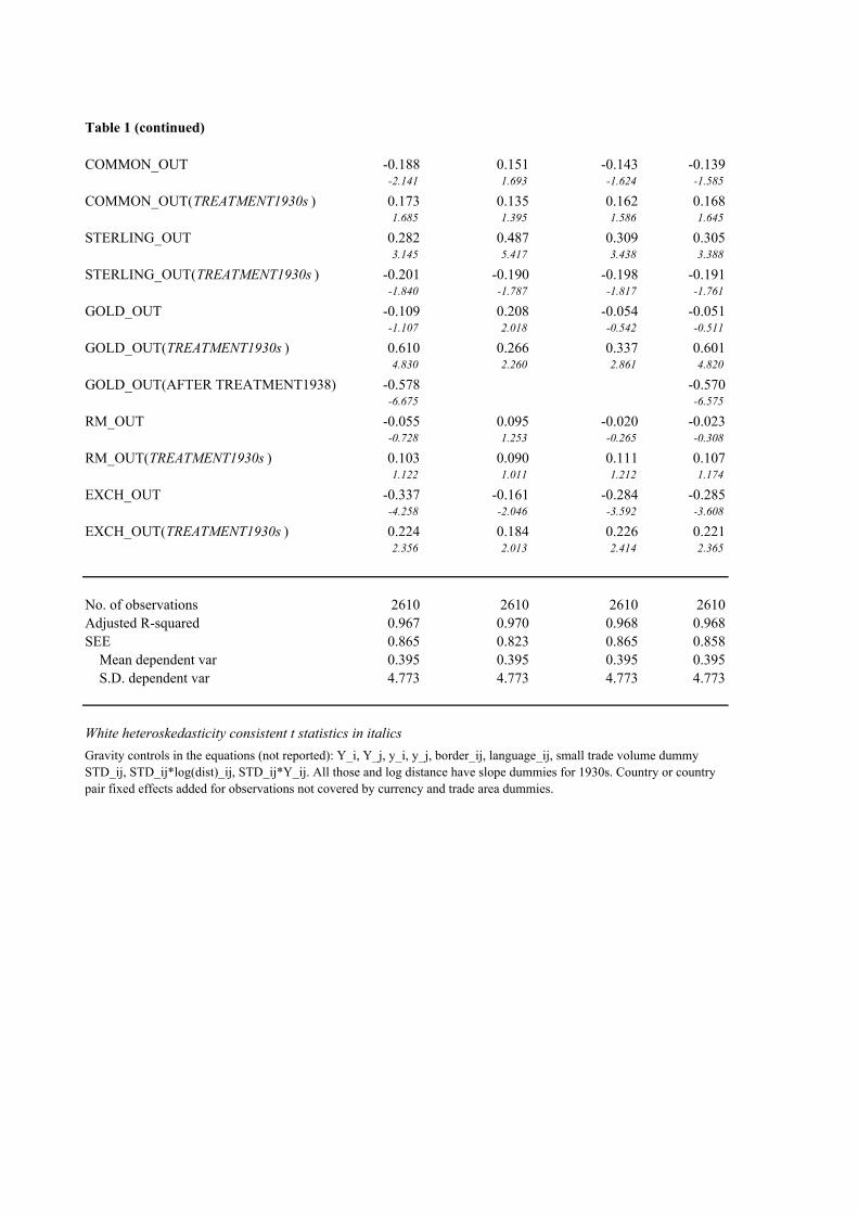
Table 1 (continued)

COMMON_OUT -0.188 0.151 -0.143 -0.139-2.141 1.693 -1.624 -1.585

COMMON_OUT(TREATMENT1930s ) 0.173 0.135 0.162 0.1681.685 1.395 1.586 1.645

STERLING_OUT 0.282 0.487 0.309 0.3053.145 5.417 3.438 3.388

STERLING_OUT(TREATMENT1930s ) -0.201 -0.190 -0.198 -0.191-1.840 -1.787 -1.817 -1.761

GOLD_OUT -0.109 0.208 -0.054 -0.051-1.107 2.018 -0.542 -0.511

GOLD_OUT(TREATMENT1930s ) 0.610 0.266 0.337 0.6014.830 2.260 2.861 4.820

GOLD_OUT(AFTER TREATMENT1938) -0.578 -0.570-6.675 -6.575

RM_OUT -0.055 0.095 -0.020 -0.023-0.728 1.253 -0.265 -0.308

RM_OUT(TREATMENT1930s ) 0.103 0.090 0.111 0.1071.122 1.011 1.212 1.174

EXCH_OUT -0.337 -0.161 -0.284 -0.285-4.258 -2.046 -3.592 -3.608

EXCH_OUT(TREATMENT1930s ) 0.224 0.184 0.226 0.2212.356 2.013 2.414 2.365

No. of observations 2610 2610 2610 2610Adjusted R-squared 0.967 0.970 0.968 0.968SEE 0.865 0.823 0.865 0.858 Mean dependent var 0.395 0.395 0.395 0.395 S.D. dependent var 4.773 4.773 4.773 4.773

White heteroskedasticity consistent t statistics in italicsGravity controls in the equations (not reported): Y_i, Y_j, y_i, y_j, border_ij, language_ij, small trade volume dummy STD_ij, STD_ij*log(dist)_ij, STD_ij*Y_ij. All those and log distance have slope dummies for 1930s. Country or country pair fixed effects added for observations not covered by currency and trade area dummies.

Table 2: Endogeneity of Inter-war Currency Blocks, Trade Creation Model, Panel 1928-1938

log of zero-volume adjusted trade log of trade

OLS with controls for small-scale bias Tobit OLS Tobit OLS Tobit OLScountry country pair country pair

fixed effects fixed effects fixed effects country fixed effects

LOG(DIST) -0.377 -0.585 -0.501 -0.482 -0.454 -0.658 -0.601 -0.601 -0.530-9.791 -10.557 -9.575 -10.735 -11.364 -11.831 -11.428 -10.879 -10.391

LOG(DIST)(TREATMENT1930s) -0.121 -0.063 -0.097 -0.169 -0.094 -0.131 -0.099 -0.162 -0.131-2.950 -2.290 -3.277 -3.413 -2.240 -3.979 -3.046 -4.717 -3.895

CU_IN 0.635 0.686 0.5283.684 4.898 4.328

CU_IN(TREATMENT1930s) 0.032 0.038 0.0320.410 0.448 0.370

COMMON_IN 0.694 1.656 1.819 1.075 1.002 2.261 2.060 2.483 2.2522.562 5.139 5.671 3.808 8.107 6.879 6.149 8.061 7.114

COMMON_IN(TREATMENT 1930s ) 0.488 0.477 0.314 0.573 -0.253 0.565 0.509 0.364 0.3131.393 1.334 0.843 1.545 -1.600 1.556 1.350 1.001 0.823

STERLING_IN 0.723 1.277 0.798 0.939 1.278 1.1906.586 9.711 6.026 3.490 9.325 8.989

STERLING_IN(TREATMENT1930s ) -0.208 -0.206 -0.256 0.836 -0.244 -0.253-1.507 -1.644 -1.517 2.485 -1.636 -1.723

GOLD_IN 0.105 0.414 0.049 -0.060 0.456 0.3801.013 2.244 0.453 -0.706 2.776 2.358

GOLD_IN(TREATMENT1930s ) 0.441 0.395 0.453 0.121 0.389 0.3443.715 2.928 3.553 1.258 3.128 2.470

RM_IN 0.821 0.863 0.953 0.559 1.054 0.9438.228 6.365 8.441 4.733 7.791 7.287

RM_IN(TREATMENT1930s ) -0.051 -0.071 -0.099 -0.430 -0.104 -0.083-0.378 -0.522 -0.649 -3.261 -0.823 -0.674

EXCH_IN -0.127 0.030 -0.107 0.089 0.163 0.043-1.690 1.947 -1.231 0.728 1.359 0.376

EXCH_IN(TREATMENT1930s ) 0.136 0.147 0.167 0.289 0.178 0.1801.514 1.686 1.557 2.091 1.868 1.846

No. of observations 2610 2610 2610 2136 2136 2136 2136 2136 2136Degrees of freedom 2579 2282 2288 2081 1867 1873Adjusted R-squared 0.969 0.986 0.981 0.747 0.780 0.861 0.875 0.845 0.859Mean dependent var 0.395 0.395 0.395 2.526 2.526 2.526 2.526 2.526 2.526SEE 0.839 0.612 0.653 0.843 141.554 0.900 0.634 0.661 0.672Censored obs. 229 229 229t statistics in italicsGravity controls (not reported) as in Table 1

country pair fixed effects

Table 3: Predicting Currency Bloc Membership from Binary Probit Model of Trade in 1928

Gold Bloc Commonwlth Sterling Bloc ExchCtrl Bloc RM Bloc

LOG(DIST) -1.581 0.828 0.378 -0.997 -0.270-3.784 3.328 2.713 -6.489 -0.911

LOG(TRADE 1928) 0.155 0.641 0.306 -0.197 0.9080.597 2.398 1.884 -2.240 4.495

LOG(TRADE 1928)*FR -0.054 -4.114 -4.322 -5.924 -2.891-0.430 0.000 0.000 0.000 0.000

LOG(TRADE 1928)*UK -2.597 0.297 0.757 -0.614 -2.2020.000 2.410 6.268 -4.545 0.000

LOG(TRADE 1928)*GE -2.672 -2.365 -2.249 0.120 0.3110.000 0.000 0.000 2.009 3.525

BORDER -1.856 1.002 0.814 -0.352 -0.589-2.415 1.265 1.690 -1.365 -1.637

BORDER*GE -6.613 -8.151 -1.572 -0.3320.000 0.000 -5.711 -0.749

LANGUAGE 1.347 -0.276 -1.136 0.7321.586 -0.618 -1.839 1.231

McFadden R-squared 0.570 0.641 0.580 0.390 0.539Log likelihood -40.951 -34.206 -104.301 -249.583 -77.641Restr. log likelihood -95.224 -95.224 -248.347 -409.201 -168.264LR statistic (19/18 df) 108.546 122.035 288.092 319.236 181.247Hannan-Quinn criter. 0.178 0.162 0.328 0.662 0.266

Obs. w/ depvar = 1 20 20 72 156 42Pred. as depvar = 1 [cutoff p = 0.4] 10 11 50 97 19% correct 50.0 55.0 69.4 62.18 45.24

Obs. w/ depvar = 0 850 850 798 714 828Pred. as depvar = 0 847 847 779 627 813% correct 99.7 99.7 97.6 87.82 98.2

z statistics in italicscontrols (nor reported): gravity eq., small-trade bias, GL index, country dummies for USSR, US, Argentina, Japan

Table 4: Treatment Effects Relative to Control Groups, Trade Creation Model, 1930s

log of zero-volume adjusted trade log of trade

OLS with controls for small-scale bias Tobitcountry country pair country country pair

fixed effects fixed effects fixed effects fixed effects

LOG(DIST) -0.552 -0.414 -0.659 -0.450283-19.706 -14.338 -18.782 -13.4873

GOLD BLOCREFERENCE GROUP 0.684 0.822 0.768 0.934

1.778 2.094 1.948 2.325TREATMENT EFFECT -0.062 -0.055 -0.116 -0.091

-0.158 -0.138 -0.291 -0.225REFERENCE GROUP_1938 -0.728 -0.801 -0.804 -0.903

-1.525 -1.631 -1.662 -1.812

TREATMENT EFFECT_1938 0.636 0.623 0.654 0.6341.308 1.248 1.329 1.257

COMMONWEALTHREFERENCE GROUP 0.960 0.728 2.251 1.732

1.972 1.690 11.379 8.270

TREATMENT EFFECT 0.189 0.238 -0.644 -0.4350.353 0.486 -2.101 -1.323

STERLING BLOCREFERENCE GROUP 0.148 -0.090 0.406 0.000

1.014 -0.654 1.832 0.001

TREATMENT EFFECT 0.356 0.462 0.236 0.4742.256 3.041 1.018 2.084

EXCHANGE CONTROL BLOCREFERENCE GROUP 0.013 0.052 0.050 0.088

0.205 0.840 0.662 1.155

TREATMENT EFFECT 0.051 0.041 0.019 0.0020.761 0.594 0.229 0.026

REICHSMARK BLOCREFERENCE GROUP 1.016 1.032 1.271 1.278

6.721 6.899 8.464 8.536

TREATMENT EFFECT -0.164 -0.129 -0.312 -0.271-0.956 -0.760 -1.787 -1.546

No. of observations 1740 1740 1421 1421Degrees of freedom 1713 1711 1398 1396Adjusted R-squared 0.973 0.970 0.729 0.684Mean dependent var 0.172 0.172 2.278 2.278SEE 0.763 0.809 0.807 0.873Censored obs. 172 172

Reference group includes control group and treatedt statistics in italicsGravity controls (not reported) as in Table 1

Table 5: Endogeneity of Europe's Postwar Institutions, Full Model, Panel 1928-1938

Dependent variable: Logarithm of zero-value adjusted trade volume Logarithm of tradeEstimation method: OLS with controls for small-scale bias Tobit

No additional fixed effects Country fixed effects Country pair fixed effects

LOG(DIST) -0.295 -0.196 -0.432 -0.312 -0.300 -0.214 -0.350 -0.243-6.996 -4.973 -10.214 -7.874 -7.061 -5.382 -7.100 -5.124

EEC OF SIX(1957)_IN 0.902 0.556 0.972 0.552 0.929 0.605 0.757 0.5317.235 4.824 8.079 4.714 7.439 5.254 5.231 4.073

EU OF FIFTEEN(2000)_IN 0.137 0.348 0.113 0.465 0.134 0.359 0.090 0.2671.348 3.244 1.160 4.412 1.311 3.324 0.733 2.112

EURO ZONE_IN -0.229 -0.281 -0.266 -0.356 -0.233 -0.291 -0.274 -0.377-2.715 -3.190 -3.367 -4.188 -2.749 -3.291 -2.523 -3.298

EEC57 OF SIX (1957)_OUT 0.399 0.202 0.484 0.244 0.413 0.232 0.418 0.2846.156 3.522 7.956 4.285 6.346 4.025 5.468 4.135

EU OF FIFTEEN(2000)_OUT 0.162 0.286 0.172 0.394 0.157 0.296 0.137 0.2392.658 4.441 3.149 6.440 2.573 4.563 1.773 2.931

EURO ZONE_OUT -0.072 -0.096 -0.083 -0.155 -0.056 -0.085 -0.069 -0.104-1.143 -1.461 -1.506 -2.545 -0.892 -1.275 -0.868 -1.224

Currency Arrangements in yes no yes no yes no yes nothe EquationTreatment Effects of Currency yes no yes no yes no yes noArrangements in the Equation

No. of observations 2610 2610 2610 2610 2610 2610 2136 2136No. of left-censored observations 229 229Adjusted R-squared 0.969 0.965 0.972 0.968 0.969 0.966 0.728 0.694SEE 0.850 0.896 0.799 0.859 0.842 0.885 0.873 0.928 Mean dependent var 0.395 0.395 0.395 0.395 0.395 0.395 2.526 2.526 S.D. dependent var 4.773 4.773 4.773 4.773 4.773 4.773 1.676 1.676

t statistics from White standard errors in italics (columns 1 to 6)z statistics from Hubert-White standard errors in italics (columns 7 and 8)EEC of 6: Trade between France, Germany, Italy, Netherlands,Belgium/Luxemburg

Euro zone: Trade between EU 15 members except for Denmark and Sweden

All gravity controls have slope dummies for 1930s. Cols. 2 to 8 with fixed effects for observations not covered by currency and trade area dummies.Gravity controls in the equations (not reported): Y_i, Y_j, y_i, y_j, border_ij, language_ij, small trade volume dummy STD_ij, STD_ij*log(dist)_ij, STD_ij*Y_ij.

EU of 15: Trade between EEC countries plus Portugal, Spain, Greece, Ireland, Britain, Denmark, Sweden, Finland, and Austria

Table 6: Predicting Postwar European Integration from Binary Probit Model of Trade in 1928

EEC of Six (1957) EU of Fifteen (2000) Euro Zone

LOG(DIST) -3.979 -1.436 -1.331-3.166 -8.272 -7.082

LOG(TRADE 1928) -0.129 -0.228 -0.136-0.288 -2.124 -1.229

LOG(TRADE 1928)*FR -0.008 0.079 0.104-0.076 1.132 1.514

LOG(TRADE 1928)*UK -2.415 0.116 -0.4960.000 1.783 -4.029

LOG(TRADE 1928)*GE -0.228 0.057 0.082-1.469 0.905 1.281

BORDER -1.422 -0.683 -0.837-1.668 -1.882 -2.309

LANGUAGE -3.516 -0.912 -0.629-2.279 -2.000 -1.229

McFadden R-squared 0.750 0.556 0.519Log likelihood -22.853 -157.594 -134.746Restr. log likelihood -91.249 -354.998 -280.138LR statistic 136.792 394.807 290.784Hannan-Quinn criter. 0.153 0.530 0.466

Obs. w/ depvar = 1 20 141 95Pred. as depvar = 1 14 103 55% correct 70.0 73.1 57.9

Obs. w/ depvar = 0 695 574 620Pred. as depvar = 0 692 533 601% correct 99.6 92.9 96.9

z statistics in italicscontrols (nor reported): gravity eq., country dummies for communist rule after World War II

EEC of 6: Trade between France, Germany, Italy, Netherlands,Belgium/Luxemburg

Euro zone: Trade between EU 15 members except for Denmark and SwedenCommunist rule: USSR, Poland, Chechoslovakia, Hungary, Yugoslavia, Bulgaria, Romania

p g pAustria