end-to-end speech separation with neural networks yi luo

End-to-end Speech Separation with Neural Networks

Yi Luo

Submitted in partial fulfillment of therequirements for the degree of

Doctor of Philosophyunder the Executive Committee

of the Graduate School of Arts and Sciences

COLUMBIA UNIVERSITY

2021

© 2021

Yi Luo

All Rights Reserved

Abstract

End-to-end Speech Separation with Neural Networks

Yi Luo

Speech separation has long been an active research topic in the signal processing community with

its importance in a wide range of applications such as hearable devices and telecommunication

systems. It not only serves as a fundamental problem for all higher-level speech processing tasks

such as automatic speech recognition, natural language understanding, and smart personal

assistants, but also plays an important role in smart earphones and augmented and virtual reality

devices.

With the recent progress in deep neural networks, the separation performance has been

significantly advanced by various new problem definitions and model architectures. The most

widely-used approach in the past years performs separation in time-frequency domain, where a

spectrogram or a time-frequency representation is first calculated from the mixture signal and

multiple time-frequency masks are then estimated for the target sources. The masks are applied

on the mixture’s time-frequency representation to extract the target representations, and then

operations such as inverse short-time Fourier transform is utilized to convert them back to

waveforms. However, such frequency-domain methods may have difficulties in modeling the

phase spectrogram as the conventional time-frequency masks often only consider the magnitude

spectrogram. Moreover, the training objectives for the frequency-domain methods are typically

also in frequency-domain, which may not be inline with widely-used time-domain evaluation

metrics such as signal-to-noise ratio and signal-to-distortion ratio.

The problem formulation of time-domain, end-to-end speech separation naturally arises to tackle

the disadvantages in the frequency-domain systems. The end-to-end speech separation networks

take the mixture waveform as input and directly estimate the waveforms of the target sources.

Following the general pipeline of conventional frequency-domain systems which contains a

waveform encoder, a separator, and a waveform decoder, time-domain systems can be design in a

similar way while significantly improves the separation performance. In this dissertation, I focus

on multiple aspects in the general problem formulation of end-to-end separation networks

including the system designs, model architectures, and training objectives. I start with a

single-channel pipeline, which we refer to as the time-domain audio separation network (TasNet),

to validate the advantage of end-to-end separation comparing with the conventional

time-frequency domain pipelines. I then move to the multi-channel scenario and introduce the

filter-and-sum network (FaSNet) for both fixed-geometry and ad-hoc geometry microphone

arrays. Next I introduce methods for lightweight network architecture design that allows the

models to maintain the separation performance while using only as small as 2.5% model size and

17.6% model complexity. After that, I look into the training objective functions for end-to-end

speech separation and describe two training objectives for separating varying numbers of sources

and improving the robustness under reverberant environments, respectively. Finally I take a step

back and revisit several problem formulations in end-to-end separation pipeline and raise more

questions in this framework to be further analyzed and investigated in future works.

2

Table of Contents

List of Tables . . . . . . . . . . . . . . . . . . . . . . . . . . . . . . . . . . . . . . . . . . v

List of Figures . . . . . . . . . . . . . . . . . . . . . . . . . . . . . . . . . . . . . . . . . . ix

Acknowledgments . . . . . . . . . . . . . . . . . . . . . . . . . . . . . . . . . . . . . . . . xiii

Chapter 1: Introduction to Speech Separation . . . . . . . . . . . . . . . . . . . . . . . . . 1

1.1 The Speech Separation Problem: A Brief Overview . . . . . . . . . . . . . . . . . 1

1.2 Existing Methods for Speech Separation . . . . . . . . . . . . . . . . . . . . . . . 2

1.2.1 Non-deep-learning Methods . . . . . . . . . . . . . . . . . . . . . . . . . 2

1.2.2 Deep-learning Systems . . . . . . . . . . . . . . . . . . . . . . . . . . . . 6

1.3 Evaluation Metrics for Speech Separation Systems . . . . . . . . . . . . . . . . . . 9

1.4 Datasets for Speech Separation . . . . . . . . . . . . . . . . . . . . . . . . . . . . 10

Chapter 2: Single-channel System: Time-domain Audio Separation Network . . . . . . . . 13

2.1 LSTM-TasNet: Applicability of End-to-end Separation . . . . . . . . . . . . . . . 13

2.1.1 System Pipeline . . . . . . . . . . . . . . . . . . . . . . . . . . . . . . . . 14

2.1.2 Design of the Separation Module . . . . . . . . . . . . . . . . . . . . . . . 15

2.1.3 Experiment Configurations and Results . . . . . . . . . . . . . . . . . . . 17

2.2 Conv-TasNet: Surpassing Ideal Magnitude Time-frequency Masking . . . . . . . . 19

i

2.2.1 Modifications upon LSTM-TasNet . . . . . . . . . . . . . . . . . . . . . . 20


2.3 DPRNN-TasNet: Stronger Long Sequence Modeling Ability . . . . . . . . . . . . 34

2.3.1 Modifications upon Conv-TasNet . . . . . . . . . . . . . . . . . . . . . . . 34


2.4 Discussions . . . . . . . . . . . . . . . . . . . . . . . . . . . . . . . . . . . . . . 39

Chapter 3: Multi-channel System: Filter-and-sum Network . . . . . . . . . . . . . . . . . 41

3.1 Two-stage FaSNet: Time-domain Adaptive Beamforming . . . . . . . . . . . . . . 41

3.1.1 System Pipeline . . . . . . . . . . . . . . . . . . . . . . . . . . . . . . . . 42

3.1.2 Design of Filter Separation and Extraction Modules . . . . . . . . . . . . . 45


3.2 TAC-FaSNet: Microphone-number-invariant and Geometry-independent Processing 53

3.2.1 Modifications upon the Two-stage FaSNet . . . . . . . . . . . . . . . . . . 55


3.3 iFaSNet: Implicit Filter-and-sum with Improved Feature Extraction . . . . . . . . . 61

3.3.1 Modifications upon the TAC-FaSNet . . . . . . . . . . . . . . . . . . . . . 61


3.4 Discussions . . . . . . . . . . . . . . . . . . . . . . . . . . . . . . . . . . . . . . 66

Chapter 4: Lightweight Model Design for Speech Separation . . . . . . . . . . . . . . . . 67

4.1 Related Works . . . . . . . . . . . . . . . . . . . . . . . . . . . . . . . . . . . . . 67

4.2 GC3: Group Communication with Context Codec for Ultra-lightweight Long Se-quence Modeling . . . . . . . . . . . . . . . . . . . . . . . . . . . . . . . . . . . 69

ii

4.2.1 Design of GC3 Module . . . . . . . . . . . . . . . . . . . . . . . . . . . . 70


4.3 Discussions . . . . . . . . . . . . . . . . . . . . . . . . . . . . . . . . . . . . . . 81

Chapter 5: Training Objectives for Speech Separation . . . . . . . . . . . . . . . . . . . . 82

5.1 Related works . . . . . . . . . . . . . . . . . . . . . . . . . . . . . . . . . . . . . 82

5.1.1 Training Methods for Separating Varying Numbers of Sources . . . . . . . 82

5.1.2 Training Methods for Separation in Reverberant Environments . . . . . . . 83

5.2 A2PIT: Separating Varying Numbers of Sources . . . . . . . . . . . . . . . . . . . 83

5.2.1 Motivation and Design . . . . . . . . . . . . . . . . . . . . . . . . . . . . 85

5.2.2 Detection of Invalid Outputs . . . . . . . . . . . . . . . . . . . . . . . . . 86


5.3 A2T: Distortion-controlled Separation in Noisy Reverberant Environments . . . . . 91

5.3.1 Motivation and Design . . . . . . . . . . . . . . . . . . . . . . . . . . . . 92


5.4 Discussions . . . . . . . . . . . . . . . . . . . . . . . . . . . . . . . . . . . . . . 102

Chapter 6: Rethinking the Problem Formulations of End-to-end Speech Separation . . . . . 104

6.1 Rethinking the Roles of Separation Layers in Speech Separation Networks . . . . . 104

6.1.1 Motivation and Experiment Design . . . . . . . . . . . . . . . . . . . . . . 104

6.1.2 Results and Discussions . . . . . . . . . . . . . . . . . . . . . . . . . . . 108

6.2 Empirical Analysis of Generalized Iterative Speech Separation Networks . . . . . . 111



iii

6.3 Empirical Analysis of the Effect of Separation Network Components under a Time-domain Training Objective . . . . . . . . . . . . . . . . . . . . . . . . . . . . . . 117



Conclusion and Future Works . . . . . . . . . . . . . . . . . . . . . . . . . . . . . . . . . . 129

References . . . . . . . . . . . . . . . . . . . . . . . . . . . . . . . . . . . . . . . . . . . . 158

iv

List of Tables

2.1 SI-SDR (dB) and SDR (dB) for different methods on WSJ0-2mix dataset. . . . . . 17

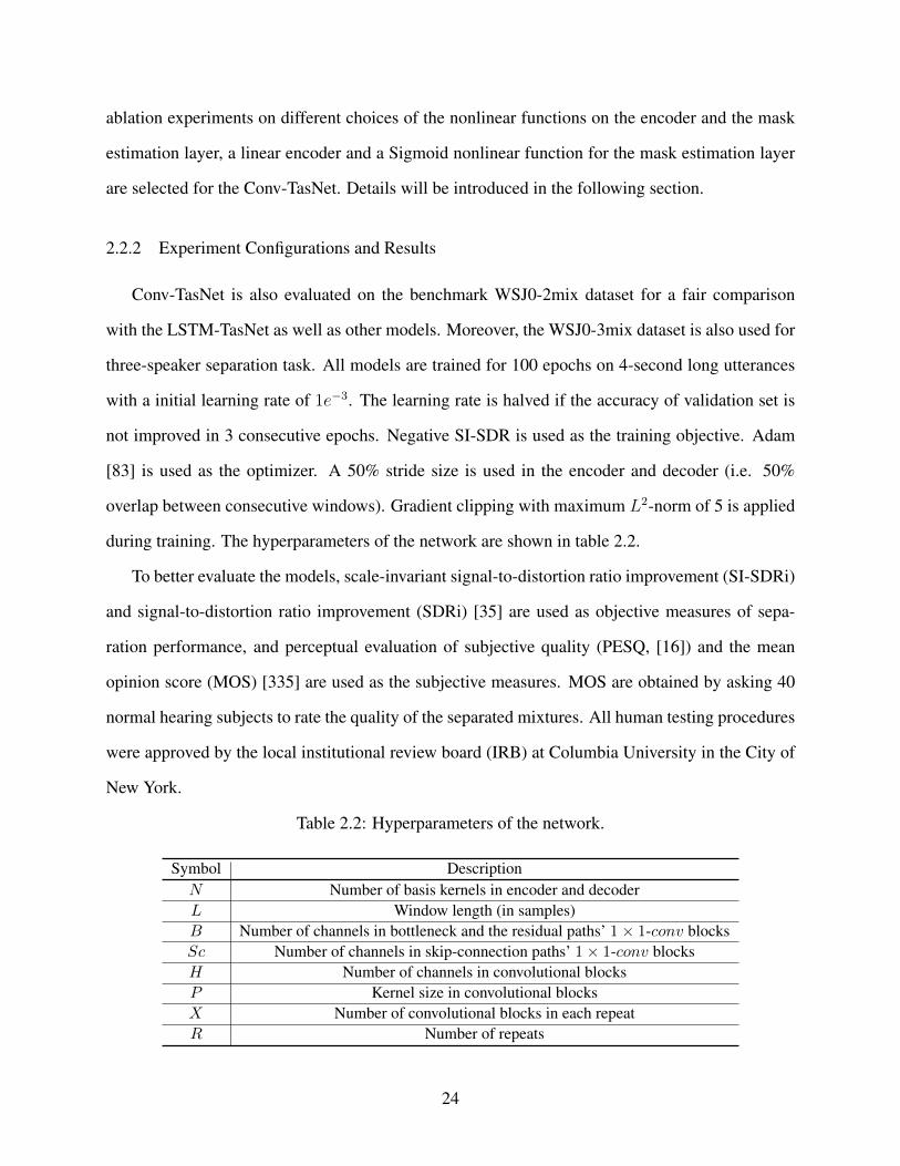
2.2 Hyperparameters of the network. . . . . . . . . . . . . . . . . . . . . . . . . . . . 24

2.3 Separation performance for different system configurations. SI-SDRi and SDRiare reported on decibel scale. . . . . . . . . . . . . . . . . . . . . . . . . . . . . . 26

2.4 The effect of different configurations in Conv-TasNet. “Norm” stands for the nor-malization method and “RF” stands for the receptive field. SI-SDRi and SDRi arereported on decibel scale. . . . . . . . . . . . . . . . . . . . . . . . . . . . . . . . 27

2.5 Comparison between Conv-TasNet and other methods on WSJ0-2mix dataset. SI-SDRi and SDRi are reported on decibel scale. . . . . . . . . . . . . . . . . . . . . 28

2.6 Comparison between Conv-TasNet and other systems on WSJ0-3mix dataset. SI-SDRi and SDRi are reported on decibel scale. . . . . . . . . . . . . . . . . . . . . 28

2.7 PESQ scores for the ideal T-F masks and Conv-TasNet on the entire WSJ0-2mixand WSJ0-3mix test sets. . . . . . . . . . . . . . . . . . . . . . . . . . . . . . . . 30

2.8 Mean opinion score (MOS, N=40) and PESQ for the 25 random selected utterancesfrom the WSJ0-2mix test set. . . . . . . . . . . . . . . . . . . . . . . . . . . . . . 30

2.9 Comparison of Conv-TasNet and different configurations of DPRNN-TasNet. SI-SDRi and SDRi are reported on decibel scale. . . . . . . . . . . . . . . . . . . . . 39

2.10 Comparison with other methods on WSJ0-2mix. SI-SDRi and SDRi are reportedon decibel scale. . . . . . . . . . . . . . . . . . . . . . . . . . . . . . . . . . . . . 39

2.11 SI-SDRi and WER results for noisy reverberant separation and recognition task.Window size is set to 32 samples for both models, and the chunk size is set to 100frames for DPRNN-TasNet. WER is calculated for both separated speakers. . . . . 40

3.1 Hyperparameters in two-stage FaSNet. . . . . . . . . . . . . . . . . . . . . . . . . 48

v

3.2 Performance of oracle beamformers. SI-SDRi is reported on decibel scale. CC:close-condition (development) set. OC: open-condition (evaluation) set. . . . . . . 50

3.3 Performance of oracle beamformers with different segment sizes for spatial covari-ance estimation. SI-SDRi is reported on decibel scale only on the OC set. . . . . . 50

3.4 Dependence of SI-SDRi on frame size for a 2-ch two-stage FaSNet in the ESE task. 51

3.5 Performance of two-stage FaSNet and tandem system in both ESE and ESS tasks. . 52

3.6 Performance of two-stage FaSNet on CHiME-3 evaluation dataset. SI-SDRi isreported on decibel scale. . . . . . . . . . . . . . . . . . . . . . . . . . . . . . . . 53

3.7 Performance of two-stage FaSNet on CHiME-3 evaluation dataset of real record-ings. WER is reported. . . . . . . . . . . . . . . . . . . . . . . . . . . . . . . . . 53

3.8 Experiment results on ad-hoc array with various numbers of microphones. SI-SDRi is reported on decibel scale. . . . . . . . . . . . . . . . . . . . . . . . . . . 60

3.9 Experiment results on 6-mic fixed geometry (circular) array. SI-SDRi is reportedon decibel scale. . . . . . . . . . . . . . . . . . . . . . . . . . . . . . . . . . . . . 60

3.10 Experiment results with various model configurations. SI-SDRi is reported ondecibel scale. . . . . . . . . . . . . . . . . . . . . . . . . . . . . . . . . . . . . . 65

3.11 Training and inference speeds of different model configurations. The speeds aremeasured on a single NVIDIA TITAN Pascal graphic card with a batch size of 4. . 66

4.1 Hyperparameters and their notations in GC3-related architectures. . . . . . . . . . 75

4.2 Comparison of DPRNN, GroupComm-DPRNN and GC3-DPRNN TasNet modelswith different hyperparameter configurations. MACs are calculated on 4-secondmixtures. . . . . . . . . . . . . . . . . . . . . . . . . . . . . . . . . . . . . . . . . 76

4.3 Comparison of GC3-DPRNN models with different model architectures for Group-Comm. . . . . . . . . . . . . . . . . . . . . . . . . . . . . . . . . . . . . . . . . . 77

4.4 Effect of group overlap ratio on model complexity and separation performance inGC3-DPRNN models. . . . . . . . . . . . . . . . . . . . . . . . . . . . . . . . . . 78

4.5 Comparison of DPRNN, TCN, Sudo rm -rf, and DPTNet architectures with andwithout GC3. The training and inference phase statistics are evaluated with a batchsize of 4. . . . . . . . . . . . . . . . . . . . . . . . . . . . . . . . . . . . . . . . . 79

vi

5.1 Confusion matrix for speaker counting for models trained for clean separation task. 89

5.2 Confusion matrix for speaker counting for models trained for noisy separation task. 89

5.3 Separation performance of various configurations on the clean separation task. SI-SDR is reported for one speaker utterances on decibel scale, and SI-SDRi is re-ported for the rest on decibel scale. . . . . . . . . . . . . . . . . . . . . . . . . . . 90

5.4 Separation performance of various configurations on the noisy separation task. SI-SDRi is reported in decibel scale. . . . . . . . . . . . . . . . . . . . . . . . . . . . 91

5.5 Comparison of DPRNN-TasNet models with objectives with and without A2T onthe noisy reverberant separation task. “OR” stands for the overlap ratio betweenthe two speakers. . . . . . . . . . . . . . . . . . . . . . . . . . . . . . . . . . . . 100

5.6 Comparison of WER from models trained with SNR with and without A2T. “OR”stands for the overlap ratio between the two speakers. . . . . . . . . . . . . . . . . 100

5.7 Comparison of DPRNN-TasNet models with direct-path RIR filter defined as the±20 ms of the first peak in the RIR filter. . . . . . . . . . . . . . . . . . . . . . . . 102

5.8 Comparison of WER from models trained with direct-path RIR filter defined as the±20 ms of the first peak in the RIR filter. . . . . . . . . . . . . . . . . . . . . . . . 102

6.1 Separation performance of different configurations in the SIMO-only and mixedSIMO-SISO designs across different overlap ratios between the two speakers. SI-SDR is reported in decibel scale. . . . . . . . . . . . . . . . . . . . . . . . . . . . 109

6.2 Separation performance of different configurations in the SISO-only design acrossdifferent overlap ratios between the two speakers. SI-SDR is reported in decibelscale. . . . . . . . . . . . . . . . . . . . . . . . . . . . . . . . . . . . . . . . . . . 110

6.3 Experiment results for different configurations in the iterative separation pipeline. . 114

6.4 Effect of layer-wise training objective. . . . . . . . . . . . . . . . . . . . . . . . . 115

6.5 Effect of iteration-specific SIMO modules with STFT/ISTFT. . . . . . . . . . . . . 116

6.6 Effect of different number of inference iterations and oracle bias information. . . . 116

6.7 Experiment results for learnable encoder/decoder with different configurations. . . 121

6.8 Experiment results for mag-spec configuration with different configurations. . . . . 121

vii

6.9 Experiment results for complex-spec configuration with different configurations. . . 121

6.10 Effect of nonnegative and unbounded magnitude time-frequency masks with 32 mswindow size. . . . . . . . . . . . . . . . . . . . . . . . . . . . . . . . . . . . . . . 121

6.11 Effect of window functions in mag-spec configuration with unbounded magnitudeT-F masks and 32 ms window size. . . . . . . . . . . . . . . . . . . . . . . . . . . 122

viii

List of Figures

2.1 LSTM-TasNet performs end-to-end separation with a three-module design. Agated nonnegative encoder maps the input mixture waveform into a hidden rep-resentation. A separation module consists of stacked LSTM layers maps the hid-den representation to a set of multiplicative masks. The masks are then appliedto the mixture hidden representation to estimate the hidden representations of thetarget sources. A linear decoder transforms the hidden representations back to thewaveforms. . . . . . . . . . . . . . . . . . . . . . . . . . . . . . . . . . . . . . . 16

2.2 Frequency response of row vectors (i.e. basis kernels) in decoder weight P in (a)causal and (b) noncausal configurations. . . . . . . . . . . . . . . . . . . . . . . . 18

2.3 (A): The block diagram of Conv-TasNet, which follows the encoder-separator-decoder design of LSTM-Tasnet. (B): The flowchart of Conv-TasNet. A linearencoder and decoder model the waveforms and a temporal convolutional network(TCN) separation module estimates the masks based on the encoder output. Differ-ent colors in the 1-D convolutional blocks in TCN denote different dilation factors.(C): The design of the 1-D convolutional block. Each block consists of a 1×1-convoperation followed by a depthwise convolution (D − conv) operation, with non-linear activation function and normalization added between each two convolutionoperations. Two linear 1× 1−conv blocks serve as the residual path and the skip-connection path respectively. . . . . . . . . . . . . . . . . . . . . . . . . . . . . . 23

2.4 Subjective and objective quality evaluation of separated utterances in WSJ0-2mix.(A): The mean opinion scores (MOS, N = 40) for IRM, Conv-TasNet and the cleanutterance. Conv-TasNet significantly outperforms IRM (p < 1e − 16, t-test). (B):PESQ scores are higher for IRM compared to the Conv-TasNet (p < 1e−16, t-test).Error bars indicate standard error (STE) (C): MOS versus PESQ for individualutterances. Each dot denotes one mixture utterance, separated using the IRM (blue)or Conv-TasNet (red). The subjective ratings of almost all utterances for Conv-TasNet are higher than their corresponding PESQ scores. . . . . . . . . . . . . . . 30

ix

2.5 (A): SDRi of an example mixture separated using LSTM-TasNet and causal Conv-TasNet as a function of the starting point in the mixture. The performance ofConv-TasNet is considerably more consistent and insensitive to the start point. (B):Standard deviation of SDRi across all the mixtures in the WSJ0-2mix test set withvarying starting points. . . . . . . . . . . . . . . . . . . . . . . . . . . . . . . . . 32

2.6 Visualization of the encoder and decoder basis functions, encoder representation,and source masks for a sample 2-speaker mixture. The speakers are shown in redand blue. The encoder representation is colored according to the power of eachspeaker at each basis function and point in time. The basis functions are sortedaccording to their Euclidean similarity and show diversity in frequency and phasetuning. . . . . . . . . . . . . . . . . . . . . . . . . . . . . . . . . . . . . . . . . . 33

2.7 Visualization of encoder and decoder basis functions and the magnitudes of theirFFTs. The basis functions are sorted based on their pairwise Euclidean similarity. . 33

2.8 System flowchart of dual-path RNN (DPRNN). (A) The segmentation stage splitsa sequential input into chunks with or without overlaps and concatenates them toform a 3-D tensor. In the implementation, the overlap ratio is set to 50%. (B)Each DPRNN block consists of two RNNs that have recurrent connections in dif-ferent dimensions. The intra-chunk bi-directional RNN is first applied to individ-ual chunks in parallel to process local information. The inter-chunk RNN is thenapplied across the chunks to capture global dependency. Multiple blocks can bestacked to increase the total depth of the network. (C) The 3-D output of the lastDPRNN block is converted back to a sequential output by performing overlap-addon the chunks. . . . . . . . . . . . . . . . . . . . . . . . . . . . . . . . . . . . . . 35

3.1 System flowchart for the two-stage FaSNet system. The first stage estimates theframe-level beamforming filters for the reference microphone based on the nor-malized correlation correlation coefficient (NCC) feature, and the second stageuses the cleaned reference microphone signal to estimate the beamforming filtersfor all remaining microphones. Cosine similarity is used as the NCC feature. . . . . 46

3.2 Beampattern examples for two different utterances in the ESS task. . . . . . . . . . 54

3.3 Flowchart for the TAC module. A transform module is shared across all the chan-nels to transform the input at each channel via a nonlinear mapping. An averagemodule applies average-pooling across the channels and applies another nonlinearmapping. A concatenate module concatenates the outputs from the transform andaverage stages and generates channel-dependent outputs. . . . . . . . . . . . . . . 56

x

3.4 Flowcharts of variants of FaSNet models. Only one output is illustrated for thesake of simplicity. (A) The original two-stage FaSNet. (B) The two-stage FaSNetwith TAC applied to every processing block in the second stage. (C) The single-stage FaSNet. (D) The single-stage FaSNet with TAC applied to every processingblock. . . . . . . . . . . . . . . . . . . . . . . . . . . . . . . . . . . . . . . . . . 57

3.5 Flowchart for the iFaSNet architecture. The modifications to the TAC-FaSNet arehighlighted, which include (A) the use of MISO design instead of the originalMIMO design, (B) the use of implicit filtering in the latent space instead of the orig-inal explicit filtering on the waveforms, (C) the use of feature-level NCC feature forcross-channel information instead of the original sample-level NCC feature, and(D) the use of context-aware filtering instead of the original context-independentfiltering. . . . . . . . . . . . . . . . . . . . . . . . . . . . . . . . . . . . . . . . . 62

4.1 Flowcharts for (A) standard sequence processing pipeline with a large sequencemodeling module; (B) GroupComm-based pipeline, where the features are splitinto groups with a GroupComm module for inter-group communication. A smallermodule for sequence modeling is then shared by all groups; (C) GC3-based pipeline,where the sequence is first segmented into local context frames, and each contextis encoded into a single feature. The sequence of summarized features is passedto a GroupComm-based module in (B). The transformed summarized features andthe original local context frames are passed to a context decoding module and anoverlap-add operation to generate the output with the same size as the input sequence. 70

5.1 Histograms of autoencoding SI-SDR (decibel scale) in different experiment con-figurations. . . . . . . . . . . . . . . . . . . . . . . . . . . . . . . . . . . . . . . . 90

5.2 Simplified illustrations for equal-valued contours in (A) SNR metric, and (B) SI-SDR metric. . . . . . . . . . . . . . . . . . . . . . . . . . . . . . . . . . . . . . . 94

5.3 Illustration of two possible linear mappings T (1)(·) and T (2)(·). T (1)(·) denotesthe one learned with A2T with a controlled distortion on the direct-path signal xd.T (2)(·) corresponds to an unconstrained mapping where the distortion on xd can besignificant. . . . . . . . . . . . . . . . . . . . . . . . . . . . . . . . . . . . . . . . 98

xi

6.1 Flowchart of different configurations on the separation models. (A) Standard sep-aration model with a single SIMO module that estimates C target sources. (B)A SIMO module first generates C intermediate features for the C sources, and aSISO module takes each of the feature as input and estimates the target sources.(C) A SISO encoder module first generates one intermediate feature from the in-put mixture. A SISO decoder module takes the feature as input and estimates thefirst target source. The input mixture, intermediate feature, and the target sourceare passed again to the decoder module to estimate the second target source. Suchprocedure is repeated until all sources are separated. . . . . . . . . . . . . . . . . . 106

6.2 Standard pipelines for iterative speech separation networks. (A) The separationoutputs at iteration i is used as auxiliary inputs at iteration i+1. (B) An output layeris added to each layer in the network to generate intermediate separation outputs,and the training objective is applied to each of them. (C) A single-input-multi-output (SIMO) separation module first separates the mixture into either outputs orintermediate features, and K single-input-single-output (SISO) post-enhancementlayers is further applied to each of the outputs to generate the targets. (D) Thecombination of the three aforementioned pipelines. . . . . . . . . . . . . . . . . . 112

6.3 Flowchart for a standard speech separation pipeline. An encoder first transformsthe mixture into a latent representation, and a linear bottleneck layer reduces itsdimension. A single-input-multi-output (SIMO) separation module generates Cfeatures correspond to the C target sources. Each output is concatenated with theencoder output and passed to another linear bottleneck layer for dimension reduc-tion, and a single-input-single-output (SISO) module is applied to estimate either amultiplicative mask for the encoder output or the latent representation for the targetsource directly. A decoder is finally used to reconstruct the target waveforms. . . . 118

6.4 Visualization of the learned window function and its frequency response. . . . . . . 122

xii

Acknowledgements

It all started from the afternoon of December 4, 2015 - I went to LabROSA’s office to seek for

some research opportunities on music information retrieval, and I met Zhuo Chen there and

learned about his ongoing work on Deep Clustering, one of the very first successful neural

network speech separation systems. I knew nothing about neural networks at that moment, but

Zhuo still kindly offered me the chance to help him extend the application of Deep Clustering to

the task of music separation. That was the start of my career on the research of source separation.

The works I’ve done as an assistant of Zhuo have led to my very first academic conference, my

very first transaction paper, and eventually a position in NAPLab as a PhD student. I would say

that my career and life would be completely different without Zhuo’s help - not only about that

afternoon, but also about all the suggestions and advice throughout these years. Words cannot

express how grateful I am, thank you so much for all the efforts.

It is my great honor to have Prof. Nima Mesgarani to be my PhD advisor. Nima is not only a

world-class researcher but also an extremely good mentor - he always knows the best way to

mentor different students according to their own aptitudes. Working with Nima is always a

pleasure. I can clearly remember the extremely detailed help from Nima in 2017 and 2018 when I

was a newly admitted PhD student and working on the first transaction paper and the first TasNet

models. Those days allowed me to know what I should do as both a PhD student and a researcher.

After that I got a clearer idea about the general problem of speech separation and gained more

experience on managing research projects, and then Nima offered me numerous suggestions on

xiii

how to become an independent researcher and gave me enough freedom to work on the problems

that I personally feel interesting. I would not be what I am now without all the efforts from Nima,

and I can say that NAPLab is the best place for me and I am really fortunate to be a member here

and being mentored by Nima.

I would like to thank the committee for my PhD defense: Prof. John Wright, Prof. Nima

Mesgarani, Prof. John Paisley, Prof. Julia Hirschberg, and Prof. Shih-Chii Liu, for your time,

encouragement, and insightful comments. I would like to also say thank you to all my

collaborators. Dr. Jonathan Le Roux and Dr. John Hershey, thank you for being my very first

collaborators and guided me to the world of source separation, I was really lucky enough to work

with both of you at the very beginning of my career. Dr. Takuya Yoshioka, thank you for

mentoring during my internship in Microsoft Research, I really enjoyed my days there and really

learned a lot from you. Prof. Shih-Chii Liu and Dr. Enea Ceolini, I really missed the days we

worked together. Really looking forward to meet you offline again and grab a beer together. Cong

Han, I have witnessed your growth as a researcher and it is really great that we have you in the lab.

NAPLab is a special place that we have people working on all different types of problems under a

same large topic - understanding how the brain processes speech, and building computational

models to analyze and mimic that. Every week’s lab meeting was always a fresh experience as we

can always expect some project from a different perspective than our own interest. I would like to

thank all our previous and current lab members for not only sharing those very interesting works

every week but also made our lab like a cozy home to stay. Zhuo, Bahar, Laura, James, Tasha,

Hassan, Rajath, Kathleen, Prachi, Menoua, Jingping, Sam, Ali, Cong, Vinay, and Xiaomin, thank

you for all the good memories in these years.

Special thanks to my parents for all the supports without asking for anything in return. I’m

returning home now, and it’s time for me to take up my duties for the family. Also special thanks

to Yuxuan Tang for supporting me throughout these year. Video chatting with you is now a daily

routine after these years, and you were always by my side in all my best memories. It’s almost the

end of the days we are apart, and let’s build more memories together in the rest of our lives.

xiv

Covid-19 had a significant influence on the world. I never thought before 2019 that I will spend

one and a half year working towards my PhD in my bedroom in China, and I never thought that

the ASRU 2019 workshop in Singapore was the last place I met Nima in person. This is an

unexpected experience for me and a hard time for the entire world. Thanks to Nima again for his

considerations on this situation and allowing me to work and even graduate remotely, and thanks

to Jingping on helping me with the packing and shipping of my belongings in NYC. Hope that the

world will return to normalcy soon.

xv

Chapter 1: Introduction to Speech Separation

In this chapter I will provide an introduction to the task of speech separation. I will first

make a brief overview on the non-deep-learning speech separation algorithms and methods, and

then show how recent developments on neural networks can either be applied to the conventional

algorithms or propose new problem formulations to the task. I will then introduce the commonly

used evaluation metrics and datasets for speech separation.

1.1 The Speech Separation Problem: A Brief Overview

The problem of speech separation has been investigated for decades [9], [19], [22], [25], [27],

[41], [215]. Its problem formulation is straightforward and simple: given a set of observations of

mixture signals {ym}Mm=1 where M denotes the number of channels or microphones available, C

target sources {xc}Cc=1 should be extracted or separated from the mixture signals. With a standard

assumption of additive sources, each mixture yi contains its observation of all the sources with an

optional additive noise signal:

ym =C∑c=1

xmc + nm (1.1)

where xmc and nm denote the c-th target source and the additive noise observed by them-th channel,

respectively. Depending on the number of available channels M , the speech separation problem

can be categorized into single-channel separation (M = 1) or multi-channel separation (M > 1).

The target sources {xc}Cc=1 can either be their observations in a certain channel, e.g., {x1c}Cc=1, or

the modulated signals generated from the target sources from all channels, e.g., via beamforming

algorithms [20], [38], [66], [142].

Real-world environments typically contain reverberations. A common definition of target

1

sources included both the direct-path signal, early reverberation signal, and the late reverbera-

tion signal, which requires the speech separation system to separation all signals that are directly

related to or generated by the clean target signal. For the task of joint speech separation and dere-

verberation, either the direct-path signal or the sum of direct-path signal and early reverberation

signal can be used as the target sources. In this dissertation, we assume that the late reverberation

is always included in the target sources except for certain methods in Chapter 3 and 5.

1.2 Existing Methods for Speech Separation

Due to the recent development of neural networks, speech separation systems can now be

broadly categorized by whether a deep neural network is applied. I first make an overview on

the methods that do not explicitly use neural networks, and then introduce the literature on deep

learning systems.

1.2.1 Non-deep-learning Methods

Non-deep-learning algorithms proposed for the speech separation problem can be roughly cat-

egorized into three categories: statistical methods, clustering methods, and factorization methods.

1. In statistical methods, the target speech signal is modeled with probability distributions such

as generalized Gaussian distributions [43], [46], [152], [178], [189] or methods such as inde-

pendent component analysis (ICA) [12], [21], [26], [37], [39], [56] and independent vector

analysis (IVA) [31], [40], [54], [70], [85], [141], [320], where the interference signal is

assumed to be statistically independent from the target speech. Maximum likelihood estima-

tion method is typically applied based on the known statistical distributions of the target.

A standard problem formulation for an ICA system is as follows. The mixture signal ym is

rewritten as the weighted summation of the sources {xmc }Cc=1:

ym =C∑c=1

hmc xmc (1.2)

2

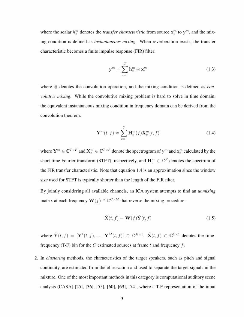
where the scalar hmc denotes the transfer characteristic from source xmc to ym, and the mix-

ing condition is defined as instantaneous mixing. When reverberation exists, the transfer

characteristic becomes a finite impulse response (FIR) filter:

ym =C∑c=1

hmc ~ xmc (1.3)

where ~ denotes the convolution operation, and the mixing condition is defined as con-

volutive mixing. While the convolutive mixing problem is hard to solve in time domain,

the equivalent instantaneous mixing condition in frequency domain can be derived from the

convolution theorem:

Ym(t, f) ≈C∑c=1

Hmc (f)Xm

c (t, f) (1.4)

where Ym ∈ CT×F and Xmc ∈ CT×F denote the spectrogram of ym and xmc calculated by the

short-time Fourier transform (STFT), respectively, and Hmc ∈ CF denotes the spectrum of

the FIR transfer characteristic. Note that equation 1.4 is an approximation since the window

size used for STFT is typically shorter than the length of the FIR filter.

By jointly considering all available channels, an ICA system attempts to find an unmixing

matrix at each frequency W(f) ∈ CC×M that reverse the mixing procedure:

X(t, f) = W(f)Y(t, f) (1.5)

where Y(t, f) = [Y1(t, f), . . . ,YM(t, f)] ∈ CM×1. X(t, f) ∈ CC×1 denotes the time-

frequency (T-F) bin for the C estimated sources at frame t and frequency f .

2. In clustering methods, the characteristics of the target speakers, such as pitch and signal

continuity, are estimated from the observation and used to separate the target signals in the

mixture. One of the most important methods in this category is computational auditory scene

analysis (CASA) [25], [36], [55], [60], [69], [74], where a T-F representation of the input

3

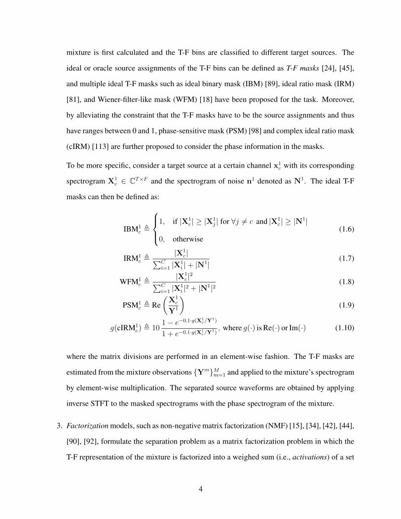
mixture is first calculated and the T-F bins are classified to different target sources. The

ideal or oracle source assignments of the T-F bins can be defined as T-F masks [24], [45],

and multiple ideal T-F masks such as ideal binary mask (IBM) [89], ideal ratio mask (IRM)

[81], and Wiener-filter-like mask (WFM) [18] have been proposed for the task. Moreover,

by alleviating the constraint that the T-F masks have to be the source assignments and thus

have ranges between 0 and 1, phase-sensitive mask (PSM) [98] and complex ideal ratio mask

(cIRM) [113] are further proposed to consider the phase information in the masks.

To be more specific, consider a target source at a certain channel x1c with its corresponding

spectrogram X1c ∈ CT×F and the spectrogram of noise n1 denoted as N1. The ideal T-F

masks can then be defined as:

IBM1c ,

1, if |X1

c | ≥ |X1j | for ∀j 6= c and |X1

c | ≥ |N1|

0, otherwise(1.6)

IRM1c ,

|X1c |∑C

i=1 |X1i |+ |N1|

(1.7)

WFM1c ,

|X1c |2∑C

i=1 |X1i |2 + |N1|2

(1.8)

PSM1c , Re

(X1c

Y1

)(1.9)

g(cIRM1c) , 10

1− e−0.1·g(X1c/Y

1)

1 + e−0.1·g(X1c/Y

1), where g(·) is Re(·) or Im(·) (1.10)

where the matrix divisions are performed in an element-wise fashion. The T-F masks are

estimated from the mixture observations {Ym}Mm=1 and applied to the mixture’s spectrogram

by element-wise multiplication. The separated source waveforms are obtained by applying

inverse STFT to the masked spectrograms with the phase spectrogram of the mixture.

3. Factorization models, such as non-negative matrix factorization (NMF) [15], [34], [42], [44],

[90], [92], formulate the separation problem as a matrix factorization problem in which the

T-F representation of the mixture is factorized into a weighed sum (i.e., activations) of a set

4

of basis signals:

W1,H1 = argminW1,H1

D(|Y1|,W1H1), s.t.W1,H1 ≥ 0 (1.11)

where W1 ∈ RT×K and H1 ∈ RK×F denote the nonnegative basis matrix and the nonneg-

ative activation matrix, respectively, and D(A,B) denotes a distance measure between the

two matrices A and B. K denotes the number of basis signals and also puts constraint on

the rank of the two matrices. Dictionary learning methods can be applied to learn the basis

signals W1 in advance [64], [65], [75], [77], and equation 1.11 is modified to only estimate

the activation matrix H1:

H1 = argminH1

D(|Y1|,W1H1), s.t.H1 ≥ 0 (1.12)

Sparsity constraints can also be enforced on the activation matrix H1 [13], [17], [28], [32],

[33], [106]:

H1 = argminH1

D(|Y1|,W1H1) + λ|H1|1, s.t.H1 ≥ 0 (1.13)

where | · |1 denotes the L1 norm and λ ∈ R denotes the weight of the sparsity term in

the optimization objective. The multi-channel extension to single-channel NMF is typically

formulated in complex-domain, and the basis signals are modified to include the spatial

properties of the different channels [50], [62], [63], [72], [103], [191].

Another important method for multi-channel speech separation is beamforming or spatial fil-

tering methods [5], [7], [14], [23], [53], [142]. A beamforming algorithm estimates M filters for

the M mixture observations to extract a target source by enhancing the signal coming from the

direction of the target source and filtering out the interference signals in other directions. The most

widely-used configuration is the linear filter-and-sum beamformer operated in frequency domain,

which has the same formulation as equation 1.5 where W(f) denotes the beamforming filter coeffi-

5

cients for all theC sources. Various filter-and-sum beamformers, such as the multi-channel Wiener

filter (MWF) beamformer, minimum variance distortionless response (MVDR) beamformer, and

linearly constrained minimum variance (LCMV) beamformer, have been proposed to satisfy cer-

tain constraints and requirements on the filtered sources.

1.2.2 Deep-learning Systems

There are mainly two ways that deep neural networks can be applied to the speech separation

task. The first way is to build new pipelines that purely rely on the modeling capacity of modern

neural networks without the conventional design paradigms. Thanks to the capacity of modern

deep neural networks, conventional operations in a standard speech separation pipeline, such as

STFT and T-F masking, may not be necessary and can be implicitly done within a neural network.

Such systems typically take the mixture waveform as the input and directly estimate the waveforms

of the target sources. After the success of 1-D CNN architectures on the task of sample-level speech

synthesis [130], various 1-D CNN architectures have been proposed and compared in the task of

waveform-level speech separation [211], [240], [294].

The second way is to replace certain stages or operations in the non-deep-learning methods by

a neural network. For methods that contain iterative parameter update procedures, e.g., various

NMF algorithms, the iterations can be unfolded as different layers in a deep neural network [79],

[105], [169]. Moreover, NMF algorithms can first be applied to learn the basis signals or the acti-

vations of the target sources, and a neural network can take both the mixture signals and the NMF

outputs as inputs and perform a better separation [82], [126], [160], [203]. Neural network designs

that directly apply the nonnegativity constraints to the intermediate feature like the NMF systems

have also been proposed [163], [167]. For methods that rely on handcrafted features, e.g., CASA

systems that use pre-calculated features for T-F bin classification, the feature extraction process

can be done by neural networks and can even be jointly optimized with the clustering process

[121], [123], [140], [198]. The T-F source assignments can also be directly generated by a neural

network without an explicit clustering process [80], [102], [148], [173]. The T-F representation for

6

T-F mask calculation is typically calculated by STFT, while other learnable signal transformations

defined by neural networks can also be designed to learn better signal representations [201], [214],

[243], [266], [280], [299].

The training of neural network speech separation models typically rely on the supervised train-

ing framework, where the target speakers are used as the training labels during the training phase.

A sequential order, or permutation, is then implicitly introduced to both the system outputs and

the training labels. When additional speaker-specific information is available, the permutation of

the system outputs can be easily determined, and the corresponding training label permutation can

be set to match that of the system outputs. However, when the speaker-specific information is not

available, the system output permutation can be different from the training label permutation, and

the training can fail due to this permutation mismatch.

Two important systems, deep clustering (DPCL) [121] and permutation invariant training

(PIT) [173], were proposed to solve this permutation problem and enabled the recent advanced

of deep learning separation systems. DPCL follows the problem formulation of CASA-based ap-

proaches where T-F masks are estimated from the mixture’s spectrogram. The masks are obtained

by performing K-means clustering on a set of discriminative embeddings generated by a neural

network. Each embedding corresponds to a T-F bin, and the training objective is designed to max-

imize the similarity between the embeddings whose T-F bins are dominated by the same source,

and minimize the similarity between the embeddings whose T-F bins are dominated by different

sources:

LDPCL = |V V T − Y Y T |2W (1.14)

where V ∈ RTF×K denotes the K-dimensional embeddings for all T-F bins, Y ∈ RTF×1 is the

IBM defined in equation 1.6 representing the oracle source assignments, and | · |W denotes the

Frobenius norm of a matrix. During inference phase, the embeddings are extracted and directly

sent to the K-means algorithm to achieve the classification assignments of the T-F bins, which

7

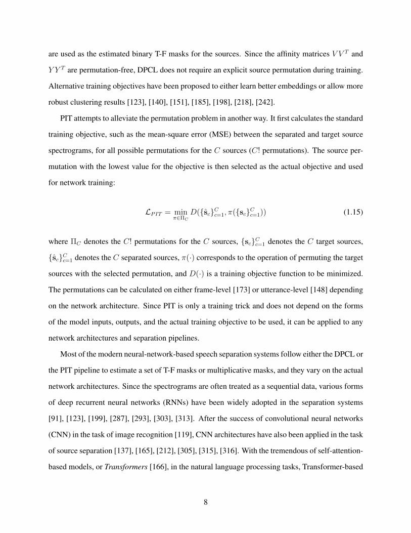
are used as the estimated binary T-F masks for the sources. Since the affinity matrices V V T and

Y Y T are permutation-free, DPCL does not require an explicit source permutation during training.

Alternative training objectives have been proposed to either learn better embeddings or allow more

robust clustering results [123], [140], [151], [185], [198], [218], [242].

PIT attempts to alleviate the permutation problem in another way. It first calculates the standard

training objective, such as the mean-square error (MSE) between the separated and target source

spectrograms, for all possible permutations for the C sources (C! permutations). The source per-

mutation with the lowest value for the objective is then selected as the actual objective and used

for network training:

LPIT = minπ∈ΠC

D({sc}Cc=1, π({sc}Cc=1)) (1.15)

where ΠC denotes the C! permutations for the C sources, {sc}Cc=1 denotes the C target sources,

{sc}Cc=1 denotes the C separated sources, π(·) corresponds to the operation of permuting the target

sources with the selected permutation, and D(·) is a training objective function to be minimized.

The permutations can be calculated on either frame-level [173] or utterance-level [148] depending

on the network architecture. Since PIT is only a training trick and does not depend on the forms

of the model inputs, outputs, and the actual training objective to be used, it can be applied to any

network architectures and separation pipelines.

Most of the modern neural-network-based speech separation systems follow either the DPCL or

the PIT pipeline to estimate a set of T-F masks or multiplicative masks, and they vary on the actual

network architectures. Since the spectrograms are often treated as a sequential data, various forms

of deep recurrent neural networks (RNNs) have been widely adopted in the separation systems

[91], [123], [199], [287], [293], [303], [313]. After the success of convolutional neural networks

(CNN) in the task of image recognition [119], CNN architectures have also been applied in the task

of source separation [137], [165], [212], [305], [315], [316]. With the tremendous of self-attention-

based models, or Transformers [166], in the natural language processing tasks, Transformer-based

8

models have also been tested on the separation task [265], [267], [268], [300]. While these sys-

tems were mainly proposed for single-channel separation, their extensions to the multi-channel or

multi-modal separation task can be straightforward by incorporating cross-channel or cross-modal

features into either the encoder or the separator module [171], [186], [219], [231], [257], [273],

[274], [304], [311].

Besides the use of cross-channel features to perform multi-channel speech separation with neu-

ral networks, conventional beamforming algorithms can also benefit from the advances in neural

source separation systems. Conventional beamforming algorithms often require a robust and ac-

curate estimation of the statistics of the target source. When the target and the interference are

partially-overlapped, this can be done by detecting the periods where only the target source is ac-

tive. However, when the two signals are fully-overlapped, the estimation of the target source can be

hard and inaccurate, resulting in a poor estimation of DOA or spatial features required to calculate

the beamforming filters. The so-called masked-based beamforming systems use the estimated T-F

masks at each channel as the estimate for the target sources for the calculation of spatial features

and beamforming filters [100], [117], [118], [122], [136], [143], [156], [157], [159], [170], [176],

[181], [188], [202], [333]. Mask-based beamforming systems have been successful in both syn-

thetic and real datasets and have been deployed to many devices and applications in the real world.

For separation systems that do not generate T-F masks, the separation outputs can also be directly

used for a selected conventional beamforming algorithm [205], [298], [319]. Moreover, the beam-

forming filters can also be directly learned by a neural network without the need of T-F masks

or conventional problem formulations of beamforming, leading to the so-called learning-based

beamforming systems [111], [125], [134], [135], [154], [161], [190], [241], [286].

1.3 Evaluation Metrics for Speech Separation Systems

The most widely-used evaluation metrics for modern speech separation systems are signal-

to-noise ratio (SNR), signal-to-distortion ratio (SDR) and scale-invariant signal-to-distortion ratio

(SI-SDR). These three metrics are designed to measure the signal quality of the separated sources

9

compared to the targets.

1. SNR between an estimated signal x and the clean target x is defined as:

SNR(x,x) = 10 log10

( ||x||22||x− x||22

)(1.16)

2. SDR has been used as a default metrics for source separation systems [35]. SDR allows

a linear distortion on the target source F(·), typically defined as the least-square mapping

between delayed versions of x and x, and is defined as:

SDR(x,x) = 10 log10

( ||F(x)||22||F(x)− x||22

)(1.17)

Existing toolboxes provide sample implementations to the metric [35], [87].

3. SI-SDR was proposed as a modification to SDR to not only address the misuse of the metric

but also improve its robustness and accuracy on the evaluation results [236]. SI-SDR is

defined as:

SI-SDR(x,x) = 10 log10

( ||αx||22||αx− x||22

)(1.18)

where α , xTx||x||22

is an optimal rescaling factor.

Beyond the three metrics, other evaluation metrics used for speech enhancement and source

separation systems such as perceptual evaluation of speech quality (PESQ) [16], short-time ob-

jective intelligibility (STOI) [58], and perceptual evaluation methods for audio source separation

(PEASS) [59], can also be applied to speech separation systems.

1.4 Datasets for Speech Separation

Most modern speech separation networks rely on simulated multi-speaker datasets for both

training and evaluation. Although different systems may create their own datasets, there are a few

10

benchmark datasets used by a variety of speech separation systems for fair performance compari-

son.

1. WSJ0-2mix [121]: WSJ0-2mix contains 30 hours of 8 kHz training data (20000 utterances)

that are generated from the Wall Street Journal (WSJ0) si_tr_s set. It also has 10 hours of

validation data (5000 utterances) and 5 hours of test data (3000 utterances) generated by

using the si_dt_05 and si_et_05 sets, respectively. Each mixture is artificially generated

by randomly selecting different speakers from the corresponding set and mixing them at

a random relative signal-to-noise ratio (SNR) between -5 and 5 dB. All the utterances are

assumed to be clean and anechoic, and all the mixtures contain a 100% overlap ratio between

the two speakers.

2. WHAM! & WHAMR! [256], [291]: The WSJ0 Hipster Ambient Mixtures (WHAM!) dataset

and its reverberant counterpart (WHAMR!) extend the anechoic and noise-free WSJ0-2mix

dataset with real-world noise and artificial reverberations. The WHAM! noise dataset is

split into 58 hours of training data (20000 utterances), 15 hours of validation data (5000

utterances), and 9 hours of test data (3000 utterances), respectively, following the original

configuration of wsj0-2mix dataset. The artificial reverberantions are generated by simulat-

ing the room impulse response (RIR) filters from random-sized rooms [208].

3. SMS-WSJ [229]: The Spatialized Multi-Speaker Wall Street Journal (SMS-WSJ) dataset

contains 33561, 982, and 1332 train, validation, and test mixtures, respectively, with highly

randomized configurations of artificial room sizes, RIR filters, and microphone and speaker

locations. It also contains truncated RIR filters that represent the early reflections and can

potentially be used for joint separation and dereverberation task.

4. LibriMix [269]: The LibriMix dataset is generated by clean speech utterances in the Lib-

rispeech dataset [109] and noise signals from WHAM!. It contains both two-speaker and

three-speaker mixtures with 170 and 186 hours of training data, respectively. It also contains

a partially-overlapped test set where the overlap ratio between the speakers are uniformly

11

sampled between 0% and 100%. This configuration is designed to mimic the realistic and

conversation-like scenarios.

5. LibriCSS [268]: The LibriCSS dataset is particularly designed for continuous speech sepa-

ration task, which is defined as the separation problem on long, unsegmented recordings. It

contains 10 hours of multi-channel audio recorded from real playbacks of utterances sam-

pled from the Librispeech dataset from a loud speaker in real meeting rooms. The recording

are split into 10 1-hour sessions, and each session is further segmented into 6 10-minute-

long mini-sessions with different overall speaker overlap ratios. Each mini-session contains

8 active speakers with a maximum overlap ratio of 40%. This dataset is purely proposed

for evaluation purpose, and the evaluation can be done at either utterance-level (with oracle

utterance boundaries) or session-level with both signal quality metrics and automatic speech

recognition accuracy.

Other public available datasets for the task of multi-talker speech recognition, e.g., the Compu-

tational Hearing in Multisource Environments (CHiME) datasets [51], [68], [73], [96], [180], can

also be used for speech separation systems. However, some of the datasets might not contain clean

target sources and the calculation of signal-quality metrics can be inaccurate, and the evaluation

of the speech separation systems in such conditions can be done by evaluating the word error rate

(WER) of the separated sources by a selected speech recognition engine.

12

Chapter 2: Single-channel System: Time-domain Audio Separation Network

In this chapter I will introduce a time-domain single-channel system, the time-domain audio

separation network (TasNet), for source separation. TasNet has a simple motivation of replac-

ing the complex-valued STFT with a real-valued, trainable module (namely the adaptive encoder

and decoder) jointly learned with the separation module, and use a time-domain training objec-

tive function to perform end-to-end optimization. According to how the adaptive encoder and

decoder and the separation module are designed, three versions of TasNet have been proposed:

the LSTM-TasNet [201] was the very first version of TasNet which validated the applicability of

such end-to-end training, the Conv-TasNet [243] was the second version of TasNet and was also

the first deep learning system that surpassed the performance of several ideal magnitude time-

frequency masks, and the DPRNN-TasNet [287] was the third version that significantly improved

the sequence modeling power and boosted the performance.

2.1 LSTM-TasNet: Applicability of End-to-end Separation

Prior to LSTM-TasNet, all state-of-the-art systems for speech separation operated on frequency

domain. LSTM-TasNet served as a step towards validating the applicability of end-to-end sepa-

ration by replacing the STFT and inverse STFT stages by learnable encoding and decoding mod-

ules, while keeping the separation module almost unchanged. Experiment results showed that

LSTM-TasNet can achieve better or on par performance comparing with other frequency-domain

networks, proving the applicability of the end-to-end separation paradigm.

13

2.1.1 System Pipeline

The problem of single-channel speech separation can be formulated in terms of estimating C

sources s1(t), . . . , sC(t) ∈ R1×T , given the discrete waveform of the mixture x(t) ∈ R1×T , where

x(t) =C∑c=1

sc(t) (2.1)

Following the same windowing process in STFT, the input mixture can be divided into over-

lapping windows of length L, represented by xk ∈ R1×L, where k = 1, . . . , T denotes the window

index and T denotes the total number of windows in the input. Instead of applying a discrete

Fourier transform on each xk, LSTM-TasNet transforms xk to a nonnegative hidden representation

via a gated layer:

xk =xk||xk||2

(2.2)

wk = ReLU(xkU)� σ(xkV) (2.3)

where wk ∈ R1×N is the hidden representation for xk, U,V ∈ RL×N are two learnable weight

matrices, ReLU(·) corresponds to the rectified linear unit function, σ(·) corresponds to the Sigmoid

function, || · ||2 denotes the L2-norm of a vector, and � denotes the Hadamard product. The L2-

norm normalization is applied to ensure that the calculation of wk is invariant to the input power.

Note that since the multiplication between xk and each column in U and V can be viewed as a

linear convolution operation, equation 2.3 can be viewed as an operation similar to DFT, and each

column in U and V can be formulated as a convolutional kernel of length L.

Given that wk is always nonnegative due to the gating operation, wk can be treated as a replace-

ment of the nonnegative magnitude spectrogram of the mixture, and C multiplicative mappings

similar to the time-frequency masks can be estimated by methods identical to the conventional

time-frequency masking systems. Given the sequence of hidden representations W ∈ RT×N , a

deep bi-directional LSTM (BLSTM) network is used as the separation module and applied on W

14

to estimateC nonnegative “multiplicative masks” Mc ∈ RT×N , , c = 1, . . . , C. The estimated hid-

den representation Sc for source c is then obtained by calculating the Hadamard product between

the mixture hidden representation W and the multiplicative mask Mc:

Sc,k = (Wk �Mc,k) · ||xk||2 (2.4)

The L2-norm of each frame is multiplied back to the masked hidden representations to reverse the

L2-norm normalization operation.

A linear transformation is finally applied to Sc to reconstruct the waveform of source c:

sc(t) = OLA(ScP) (2.5)

where P ∈ RN×L is the learnable weight matrix in the deecoder, and OLA stands for the overlap-

add operation on the neighbouring windows for waveform reconstruction.

The training objective function is the negative SI-SDR score between the separated outputs

sc(t) and the target outputs sc(t) under the permutation invariant training (PIT) framework:

L = −maxπ∈ΠC

SI-SDR({sc(t)}π, {sc(t)}) (2.6)

where {sc(t)}π denotes the permuted separated outputs {sc(t)} under the given index permuation

π, and ΠC denotes all the possible index permutations for the C sources. Figure 2.1 shows the

flowchart of LSTM-TasNet.

2.1.2 Design of the Separation Module

The separation module follows the standard design of deep recurrent networks in prior works.

A standard deep recurrent network contains stacked recurrent layers such as LSTM or GRU lay-

ers, either uni-directional or bi-directional, to capture hierarchical sequential dependencies within

the input sequence W. As the name indicates, LSTM-TasNet uses LSTM layers for sequence

15

Figure 2.1: LSTM-TasNet performs end-to-end separation with a three-module design. A gatednonnegative encoder maps the input mixture waveform into a hidden representation. A separationmodule consists of stacked LSTM layers maps the hidden representation to a set of multiplicativemasks. The masks are then applied to the mixture hidden representation to estimate the hiddenrepresentations of the target sources. A linear decoder transforms the hidden representations backto the waveforms.

modeling. A layer normalization operation is applied on the input sequence W to speed up and

stabilize the training process:

wk =g

σ⊗ (wk − µ) + b (2.7)

µ =1

N

N∑j=1

wk,j σ =

√√√√ 1

N

N∑j=1

(wk,j − µ)2 (2.8)

where parameters g ∈ R1×N and b ∈ R1×N are gain and bias vectors that are jointly optimized

with the network. This normalization step enables the separation network to be scale invariant to

the power of W, and W is used as the actual input sequence to the LSTM layers. A fully-connected

(FC) layer is applied on the output of the last LSTM layer to generate the C masks {Mc}Cc=1. A

Softmax function is used in the FC layer in order to mimic the property of T-F masks, hence the

unit summation constraint∑C

c=1 Mc = 1 satisfies. Moreover, an identity skip connection [120]

is added between every two LSTM layers in order to enhance the gradient flow and accelerate the

16

Table 2.1: SI-SDR (dB) and SDR (dB) for different methods on WSJ0-2mix dataset.

Method Causal SI-SDRi SDRiuPIT-LSTM [148] X – 7.0

LSTM-TasNet X 7.7 8.0DPCL++ [123] × 10.8 –DANet [140] × 10.5 –

uPIT-BLSTM-ST [148] × – 10.0BLSTM-TasNet × 10.8 11.1

training process.

2.1.3 Experiment Configurations and Results

LSTM-TasNet is evaluated on the benchmark WSJ0-2mix dataset described in Chapter 1.4.

The parameters of the network include the window length L, the dimension of the hidden rep-

resentation N , and the configuration of the deep LSTM separation network. Here L is set to 40

samples (5 ms at 8 kHz) and N is set to 500. The deep LSTM separation module contains 4

uni-directional or bi-directional LSTM layers, where for the uni-directional configuration there are

1000 hidden units in each layer, and for the bi-directional configuration there are 500 hidden units

in each direction. The FC layer contains 1000 hidden units that generates two 500-dimensional

multiplicative masks.

During training, the batch size is set to 128, and the initial learning rate is set to 3e−4 for the

causal system (uni-directional LSTM) and 1e−3 for the noncausal system (bi-directional LSTM).

The learning rate is halved if the performance on the validation set is not improved in 3 consecutive

epochs. The criteria for early stopping is no decrease in the cost function on the validation set for

10 epochs. Adam [83] is used as the optimization algorithm. Negative SI-SDR is used as the

training objective. No further regularization or training procedures were used.

Similar to prior works [123], [140], the curriculum training strategy [47] is applied for network

optimization. The training of the models starts on 0.5 second long utterances until convergence,

and is resumed on 4 second long utterances afterwards.

Table 2.1 shows the performance of LSTM-TasNet as well as three frequency-domain systems,

17

Deep Clustering (DPCL++, [123]), Permutation Invariant Training (PIT, [148]), and Deep Attrac-

tor Network (DANet, [140]). Here LSTM-TasNet represents the causal configuration with uni-

directional LSTM layers and BLSTM-TasNet corresponds to the system with bi-directional LSTM

layers. The best reported performance on WSJ0-2mix is reported for other systems. With causal

configuration, LSTM-TasNet significantly outperforms another frequency-domain causal system,

the uPIT model with LSTM as sequence modeling module. Under the noncausal configuration,

LSTM-TasNet outperforms all the other systems. As the deep LSTM module of LSTM-TasNet

is almost identical to the separation module in the three frequency-domain systems listed above,

the results proves the applicability of end-to-end separation comparing with frequency-domain

modeling.

(a)

(b)

Figure 2.2: Frequency response of row vectors (i.e. basis kernels) in decoder weight P in (a) causaland (b) noncausal configurations.

The decoder weight P can be treated as the basis kernels for waveform reconstruction. Fig-

ure 2.2 shows the frequency response of the basis signals in P sorted by their center frequencies

(i.e. the bin index corresponding to the the peak magnitude). There is clearly a continuous tran-

18

sition from low to high frequency, showing that the network has learned to perform a spectral

decomposition of the waveform, similar to the finding in other time-domain speech processing

systems [112]. The frequency bandwidths of the basis kernels also increase with their center fre-

quencies similar to mel-filterbanks. In contrast, the basis signals in LSTM-TasNet have a higher

resolution in lower frequencies compared to Mel and STFT. In fact, 60% of the basis signals have

center frequencies below 1 kHz, which may indicate the importance of low-frequency resolution

for accurate speech separation.

2.2 Conv-TasNet: Surpassing Ideal Magnitude Time-frequency Masking

While LSTM-TasNet already outperformed multiple frequency-domain speech separation meth-

ods in both causal and noncausal implementations, the use of the deep LSTM separation mod-

ule significantly limited its applicability. First, choosing smaller window size L in the encoder

increases the length of the mixture hidden representations T , which makes the training of the

stacked LSTM module unmanageable. Second, the large number of parameters in the deep LSTM

module significantly increases its computational cost and limits its applicability to low-resource,

low-power platforms such as wearable hearing devices. The third problem is caused by the long

temporal dependencies of LSTM networks which often results in inconsistent separation accu-

racy, for example, when changing the starting point of the mixture. To alleviate the limitations

of LSTM-TasNet, a fully-convolutional TasNet (Conv-TasNet) is proposed here that uses a convo-

lutional network for the separation module. Motivated by the success of temporal convolutional

network (TCN) models [124], [149], [179], Conv-TasNet uses stacked dilated 1-D convolutional

blocks to replace the deep LSTM networks for the separation step. The use of convolution allows

parallel processing on consecutive frames or segments to greatly speed up the separation process

and also significantly reduces the model size. To further decrease the number of parameters and

the computational cost, the original convolution operation is substituted with depthwise separable

convolution [115], [144]. With these modifications, Conv-TasNet significantly increases the sep-

aration accuracy over the LSTM-TasNet in both causal and noncausal configurations. Moreover,

19

the separation accuracy of Conv-TasNet surpasses the performance of ideal magnitude T-F masks,

including the ideal binary mask (IBM [29]), ideal ratio mask (IRM [48], [89]), and Winener filter-

like mask (WFM [98]) in both signal-to-distortion ratio (SDR) and subjective (mean opinion score,

MOS) measures.

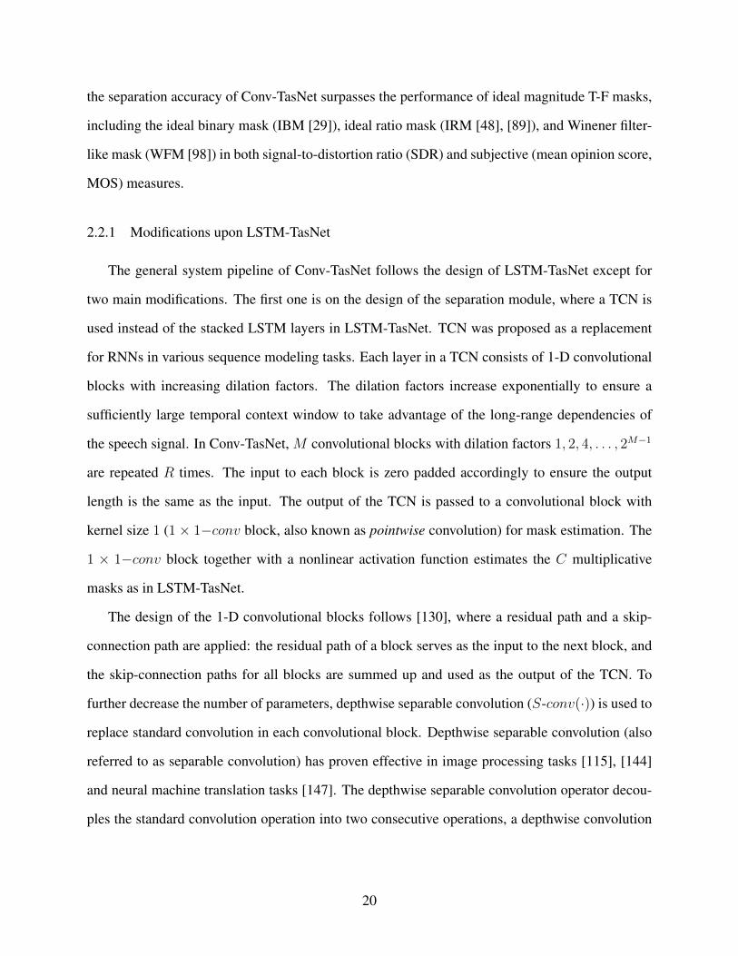
2.2.1 Modifications upon LSTM-TasNet

The general system pipeline of Conv-TasNet follows the design of LSTM-TasNet except for

two main modifications. The first one is on the design of the separation module, where a TCN is

used instead of the stacked LSTM layers in LSTM-TasNet. TCN was proposed as a replacement

for RNNs in various sequence modeling tasks. Each layer in a TCN consists of 1-D convolutional

blocks with increasing dilation factors. The dilation factors increase exponentially to ensure a

sufficiently large temporal context window to take advantage of the long-range dependencies of

the speech signal. In Conv-TasNet, M convolutional blocks with dilation factors 1, 2, 4, . . . , 2M−1

are repeated R times. The input to each block is zero padded accordingly to ensure the output

length is the same as the input. The output of the TCN is passed to a convolutional block with

kernel size 1 (1 × 1−conv block, also known as pointwise convolution) for mask estimation. The

1 × 1−conv block together with a nonlinear activation function estimates the C multiplicative

masks as in LSTM-TasNet.

The design of the 1-D convolutional blocks follows [130], where a residual path and a skip-

connection path are applied: the residual path of a block serves as the input to the next block, and

the skip-connection paths for all blocks are summed up and used as the output of the TCN. To

further decrease the number of parameters, depthwise separable convolution (S-conv(·)) is used to

replace standard convolution in each convolutional block. Depthwise separable convolution (also

referred to as separable convolution) has proven effective in image processing tasks [115], [144]

and neural machine translation tasks [147]. The depthwise separable convolution operator decou-

ples the standard convolution operation into two consecutive operations, a depthwise convolution

20

(D-conv(·)) followed by pointwise convolution (1× 1−conv(·)):

D-conv(Y,K) = concat(yj ~ kj), j = 1, . . . , N (2.9)

S-conv(Y,K,L) = D-conv(Y,K) ~ L (2.10)

where Y ∈ RG×M is the input to S-conv(·), K ∈ RG×P is the convolution kernel with size P ,

yj ∈ R1×M and kj ∈ R1×P are the rows of matrices Y and K, respectively, L ∈ RG×H×1 is

the convolution kernel with size 1, and ~ denotes the convolution operation. In other words, the

D-conv(·) operation convolves each row of the input Y with the corresponding row of matrix K,

and the 1 × 1−conv block linearly transforms the feature space. In comparison with the standard

convolution with kernel size K ∈ RG×H×P , depthwise separable convolution only contains G ×

P +G×H parameters, which decreases the model size by a factor of H×PH+P

≈ P when H � P .

A nonlinear activation function and a normalization operation are added after both the first

1 × 1-conv and D-conv blocks respectively. The nonlinear activation function is the parametric

rectified linear unit (PReLU) [99]:

PReLU(x) =

x, ifx ≥ 0

αx, otherwise(2.11)

where α ∈ R is a trainable scalar controlling the negative slope of the rectifier. The choice of the

normalization method in the network depends on the causality requirement. For noncausal config-

uration, a global layer normalization (gLN) operation is introduced to utilize the global sequence

21

information across both the channel and time dimensions:

gLN(F) =F− E[F]√V ar[F] + ε

� γ + β (2.12)

E[F] =1

NT

∑NT

F (2.13)

V ar[F] =1

NT

∑NT

(F− E[F])2 (2.14)

where F ∈ RN×T is a sequential feature, γ, β ∈ RN×1 are trainable parameters, and ε is a small

constant for numerical stability. This is identical to the standard layer normalization applied in

computer vision models where the channel and time dimension correspond to the width and height

dimension in an image [114]. In causal configuration, gLN cannot be applied since it relies on

the future values of the signal at any time step. Instead, a cumulative layer normalization (cLN)

operation is designed operation to perform step-wise normalization:

cLN(fk) =fk − E[f t≤k]√V ar[f t≤k] + ε

� γ + β (2.15)

E[f t≤k] =1

Nk

∑Nk

f t≤k (2.16)

V ar[f t≤k] =1

Nk

∑Nk

(f t≤k − E[f t≤k])2 (2.17)

where fk ∈ RN×1 is the k-th frame of the entire feature F, f t≤k ∈ RN×k corresponds to the feature

of k frames [f1, . . . , fk], and γ, β ∈ RN×1 are trainable parameters applied to all frames. To ensure

that the separation module is invariant to the scaling of the input, the selected normalization method

is applied to the encoder output w before it is passed to the separation module.

At the beginning of the separation module, a linear 1 × 1-conv block is added as a bottleneck

layer. This block determines the number of channels in the input and residual path of the subse-

quent convolutional blocks. For instance, if the linear bottleneck layer has B channels, then for

a 1-D convolutional block with H channels and kernel size P , the size of the kernel in the first

1× 1-conv block and the first D-conv block should be O ∈ RB×H×1 and K ∈ RH×P respectively,

22

and the size of the kernel in the residual paths should be LRs ∈ RH×B×1. The number of output

channels in the skip-connection path can be different than B and is denoted as LSc ∈ RH×Sc×1.

Figure 2.3 shows the flowchart of the entire system as well as the design of the 1-D convolutional

blocks.

Figure 2.3: (A): The block diagram of Conv-TasNet, which follows the encoder-separator-decoderdesign of LSTM-Tasnet. (B): The flowchart of Conv-TasNet. A linear encoder and decodermodel the waveforms and a temporal convolutional network (TCN) separation module estimatesthe masks based on the encoder output. Different colors in the 1-D convolutional blocks in TCNdenote different dilation factors. (C): The design of the 1-D convolutional block. Each block con-sists of a 1 × 1-conv operation followed by a depthwise convolution (D − conv) operation, withnonlinear activation function and normalization added between each two convolution operations.Two linear 1×1−conv blocks serve as the residual path and the skip-connection path respectively.

The second difference is the design of the encoder and the nonlinearity function in the mask

estimation layer of the separation module. LSTM-TasNet used a gated nonlinear encoder in order

to ensure that the mixture hidden representations are nonnegative. Moreover, the Softmax nonlin-

ear function was used in as the activation function in the mask estimation layer in LSTM-TasNet to

follow the unit-summation assumption in conventional magnitude T-F masks. However, whether

such assumptions are valid and lead to optimal separation performance is unknown. After multiple

23

ablation experiments on different choices of the nonlinear functions on the encoder and the mask

estimation layer, a linear encoder and a Sigmoid nonlinear function for the mask estimation layer

are selected for the Conv-TasNet. Details will be introduced in the following section.


Conv-TasNet is also evaluated on the benchmark WSJ0-2mix dataset for a fair comparison

with the LSTM-TasNet as well as other models. Moreover, the WSJ0-3mix dataset is also used for

three-speaker separation task. All models are trained for 100 epochs on 4-second long utterances

with a initial learning rate of 1e−3. The learning rate is halved if the accuracy of validation set is

not improved in 3 consecutive epochs. Negative SI-SDR is used as the training objective. Adam

[83] is used as the optimizer. A 50% stride size is used in the encoder and decoder (i.e. 50%

overlap between consecutive windows). Gradient clipping with maximum L2-norm of 5 is applied

during training. The hyperparameters of the network are shown in table 2.2.

To better evaluate the models, scale-invariant signal-to-distortion ratio improvement (SI-SDRi)

and signal-to-distortion ratio improvement (SDRi) [35] are used as objective measures of sepa-

ration performance, and perceptual evaluation of subjective quality (PESQ, [16]) and the mean

opinion score (MOS) [335] are used as the subjective measures. MOS are obtained by asking 40

normal hearing subjects to rate the quality of the separated mixtures. All human testing procedures

were approved by the local institutional review board (IRB) at Columbia University in the City of

New York.

Table 2.2: Hyperparameters of the network.

Symbol DescriptionN Number of basis kernels in encoder and decoderL Window length (in samples)B Number of channels in bottleneck and the residual paths’ 1× 1-conv blocksSc Number of channels in skip-connection paths’ 1× 1-conv blocksH Number of channels in convolutional blocksP Kernel size in convolutional blocksX Number of convolutional blocks in each repeatR Number of repeats

24

The first experiment on the configurations of Conv-TasNet is the nonnegativity of the encoder.

The non-negativity of the encoder output was enforced in [201] using a gated operation with ReLU

and Sigmoid nonlinear functions. This constraint was based on the assumption that the masking

operation on the encoder output is only meaningful when the mixture and target waveforms can be

represented with a nonnegative combination of the basis functions, since an unbounded encoder

representation may result in unbounded masks. However, by removing the nonlinear function

in the encoder, another assumption can be made: with an unbounded but highly overcomplete

representation of the mixture, a set of nonnegative masks can still be found to reconstruct the clean

sources. In this case, only U is used in the encoder and V is discarded, and the overcompleteness

of the representation, i.e. the ratio between N and L, becomes crucial. If there exist only a unique

weight feature for the mixture as well as for the sources, the non-negativity of the mask cannot be

guaranteed. Also note that in both assumptions, there is no constraint on the relationship between

the encoder and decoder basis functions U and P, meaning that they are not forced to reconstruct

the mixture signal perfectly. One way to explicitly ensure the autoencoder property is by choosing

P to be the pseudo-inverse of U (i.e. least square reconstruction). The choice of encoder/decoder

design affects the mask estimation: in the case of an autoencoder, the unit summation constraint

must be satisfied; otherwise, the unit summation constraint is not strictly required. To illustrate

this point, there are five possible encoder-decoder configurations:

1. Linear encoder with its pseudo-inverse (Pinv) as decoder, i.e. w = x(PTP)−1PT and x =

wP, with Softmax function for mask estimation.

2. Linear encoder and decoder where w = xU and x = wP, with Softmax or Sigmoid function

for mask estimation.

3. Encoder with ReLU activation and linear decoder where w = ReLU(xU) and x = wP,

with Softmax or Sigmoid function for mask estimation.

Separation performance of different configurations in table 2.3 shows that pseudo-inverse autoen-

coder leads to the worst performance, indicating that an explicit autoencoder configuration does

25

not necessarily improve the separation score in this framework. The performance of all other con-

figurations is comparable. Because linear encoder and decoder with Sigmoid function achieves a

slightly better accuracy over other methods, this configuration is used in all the following experi-

ments.

Table 2.3: Separation performance for different system configurations. SI-SDRi and SDRi arereported on decibel scale.

Encoder Mask Model size SI-SDRi SDRiPinv Softmax

1.5M

12.1 12.4

LinearSoftmax 12.9 13.2Sigmoid 13.1 13.4

ReLUSoftmax 13.0 13.3Sigmoid 12.9 13.2

The second experiment on the network configuration is on the effect of hyperparameters on the

overall performance. Table 2.4 shows the performance of the systems with different parameters,

from which several observations can be made:

(i) Encoder/decoder: Increasing the number of basis signals N in the encoder/decoder increases

the overcompleteness of the basis signals and improves the performance.

(ii) Hyperparameters in the 1-D convolutional blocks: A possible configuration consists of a

small bottleneck size B and a large number of channels in the convolutional blocks H .

This matches the observation in [207], where the ratio between the convolutional block and

the bottleneck H/B was found to be best around 5. Increasing the number of channels in

the skip-connection block improves the performance while greatly increases the model size.

Therefore, a small skip-connection block is selected as a trade-off between performance and

model size.

(iii) Number of 1-D convolutional blocks: When the receptive field is the same, deeper networks

lead to better performance, possibly due to the increased model capacity.

(iv) Size of receptive field: Increasing the size of receptive field leads to better performance,

which shows the importance of sequence modeling in the speech signal.

26

(v) Length of each segment: Shorter segment length consistently improves performance. Note

that the best system uses a filter length of only 2 ms ( Lfs

= 168000

= 0.002s), which makes it

very difficult to train a deep LSTM network with the same L due to the large number of time

steps in the encoder output.

(vi) Causality: Using a causal configuration leads to a significant drop in the performance. This

drop could be due to the causal convolution and/or the layer normalization operations.

Table 2.4: The effect of different configurations in Conv-TasNet. “Norm” stands for the normal-ization method and “RF” stands for the receptive field. SI-SDRi and SDRi are reported on decibelscale.

N L B H Sc P X R Norm Causal RF (s) Size SI-SDRi SDRi128 40 128 256 128 3 7 2 gLN × 1.28 1.5M 13.0 13.3256 40 128 256 128 3 7 2 gLN × 1.28 1.5M 13.1 13.4512 40 128 256 128 3 7 2 gLN × 1.28 1.7M 13.3 13.6512 40 128 256 256 3 7 2 gLN × 1.28 2.4M 13.0 13.3512 40 128 512 128 3 7 2 gLN × 1.28 3.1M 13.3 13.6512 40 128 512 512 3 7 2 gLN × 1.28 6.2M 13.5 13.8512 40 256 256 256 3 7 2 gLN × 1.28 3.2M 13.0 13.3512 40 256 512 256 3 7 2 gLN × 1.28 6.0M 13.4 13.7512 40 256 512 512 3 7 2 gLN × 1.28 8.1M 13.2 13.5512 40 128 512 128 3 6 4 gLN × 1.27 5.1M 14.1 14.4512 40 128 512 128 3 4 6 gLN × 0.46 5.1M 13.9 14.2512 40 128 512 128 3 8 3 gLN × 3.83 5.1M 14.5 14.8512 32 128 512 128 3 8 3 gLN × 3.06 5.1M 14.7 15.0512 16 128 512 128 3 8 3 gLN × 1.53 5.1M 15.3 15.6512 16 128 512 128 3 8 3 cLN X 1.53 5.1M 10.6 11.0

Table 2.5 compares the performance of the best configuration of Conv-TasNet with other state-

of-the-art methods on the same WSJ0-2mix dataset. For all systems, the best reported results in

the literature are listed. The numbers of parameters in different methods are based on reimple-

mentations, except for [194] which is provided by the authors. The missing values in the table

are either because the numbers were not reported in the study or because the results were calcu-

lated with a different STFT configuration. The previous LSTM-TasNet model is denoted by the

(B)LSTM-TasNet. While the BLSTM-TasNet already outperformed IRM and IBM, the noncausal

Conv-TasNet significantly surpasses the performance of all three ideal T-F masks in SI-SDRi and

27

SDRi metrics with a significantly smaller model size comparing with all previous methods. Ta-

ble 2.6 further compares the performance of Conv-TasNet with those of other systems on the

WSJ0-3mix dataset for three-speaker separation task. The noncausal Conv-TasNet system signif-

icantly outperforms all previous STFT-based systems in SDRi. While there is no prior result on

a causal algorithm for three-speaker separation, the causal Conv-TasNet significantly outperforms

even the other two noncausal STFT-based systems [123], [148].

Table 2.5: Comparison between Conv-TasNet and other methods on WSJ0-2mix dataset. SI-SDRiand SDRi are reported on decibel scale.

Method Size Causal SI-SDRi SDRiDPCL++ [123] 13.6M × 10.8 –

uPIT-BLSTM-ST [148] 92.7M × – 10.0DANet [140] 9.1M × 10.5 –

ADANet [198] 9.1M × 10.4 10.8cuPIT-Grid-RD [222] 47.2M × – 10.2CBLDNN-GAT[194] 39.5M × – 11.0

Chimera++ [218] 32.9M × 11.5 12.0WA-MISI-5 [220] 32.9M × 12.6 13.1

BLSTM-TasNet [200] 23.6M × 13.2 13.6Conv-TasNet-gLN 5.1M × 15.3 15.6uPIT-LSTM [148] 46.3M X – 7.0

LSTM-TasNet [200] 32.0M X 10.8 11.2Conv-TasNet-cLN 5.1M X 10.6 11.0

IRM – – 12.2 12.6IBM – – 13.0 13.5

WFM – – 13.4 13.8

Table 2.6: Comparison between Conv-TasNet and other systems on WSJ0-3mix dataset. SI-SDRiand SDRi are reported on decibel scale.

Method Size Causal SI-SDRi SDRiDPCL++ [123] 13.6M × 7.1 –

uPIT-BLSTM-ST [148] 92.7M × – 7.7DANet [140] 9.1M × 8.6 8.9

ADANet [198] 9.1M × 9.1 9.4Conv-TasNet-gLN 5.1M × 12.7 13.1Conv-TasNet-cLN 5.1M X 7.8 8.2

IRM – – 12.5 13.0IBM – – 13.2 13.6

WFM – – 13.6 14.0

28

The third experiment is on the joint subjective and objective evaluations of Conv-TasNet. Ta-

ble 2.7 shows the PESQ score for Conv-TasNet and IRM, IBM, and WFM, where IRM has the

highest score for both WSJ0-2mix and WSJ0-3mix dataset. However, since PESQ aims to predict

the subjective quality of speech, human quality evaluation can be considered as the ground truth.

Therefore, a psychophysics experiment is conducted in which 40 normal hearing subjects are asked

to listen and rate the quality of the separated speech sounds. Because of the practical limitations of

human psychophysics experiments, the subjective comparison of Conv-TasNet is restricted to the

ideal ratio mask (IRM) which has the highest PESQ score among the three ideal masks (table 2.7).

25 two-speaker mixture sounds as well as their separation output were randomly selected from the

two-speaker test set (WSJ0-2mix). To avoid a possible selection bias, the average PESQ scores for

the IRM and Conv-TasNet separated sounds for the selected 25 samples were ensured to equal to

the average PESQ scores over the entire test set (comparison of tables 2.7 and 2.8). The length of

each utterance was constrained to be within 0.5 standard deviation of the mean of the entire test

set. The subjects were asked to rate the quality of the clean utterances, the IRM-separated utter-

ances, and the Conv-TasNet separated utterances on the scale of 1 to 5 (1: bad, 2: poor, 3: fair, 4:

good, 5: excellent). A clean utterance was first given as the reference for the highest possible score

(i.e. 5). Then the clean, IRM, and Conv-TasNet samples were presented to the subjects in random

order. The mean opinion score (MOS) of each of the 25 utterances was then averaged over the 40

subjects.

Figure 2.4 and table 2.8 show the result of the human subjective quality test, where the MOS

for Conv-TasNet is significantly higher than the MOS for the IRM (p < 1e − 16, t-test). In

addition, the superior subjective quality of Conv-TasNet over IRM is consistent across most of

the 25 test utterances as shown in figure 2.4 (C). This observation shows that PESQ consistently

underestimates MOS for Conv-TasNet separated utterances, which may be due to the dependence

of PESQ on the magnitude spectrogram of speech [16] which could produce lower scores for time-

domain approaches.

The fourth experiment is on the sensitivity of LSTM-TasNet and Conv-TasNet on the mixture

29

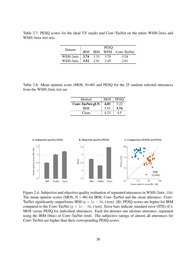
Table 2.7: PESQ scores for the ideal T-F masks and Conv-TasNet on the entire WSJ0-2mix andWSJ0-3mix test sets.

DatasetPESQ

IRM IBM WFM Conv-TasNetWSJ0-2mix 3.74 3.33 3.70 3.24WSJ0-3mix 3.52 2.91 3.45 2.61

Table 2.8: Mean opinion score (MOS, N=40) and PESQ for the 25 random selected utterancesfrom the WSJ0-2mix test set.

Method MOS PESQConv-TasNet-gLN 4.03 3.22

IRM 3.51 3.74Clean 4.23 4.5

Figure 2.4: Subjective and objective quality evaluation of separated utterances in WSJ0-2mix. (A):The mean opinion scores (MOS, N = 40) for IRM, Conv-TasNet and the clean utterance. Conv-TasNet significantly outperforms IRM (p < 1e− 16, t-test). (B): PESQ scores are higher for IRMcompared to the Conv-TasNet (p < 1e − 16, t-test). Error bars indicate standard error (STE) (C):MOS versus PESQ for individual utterances. Each dot denotes one mixture utterance, separatedusing the IRM (blue) or Conv-TasNet (red). The subjective ratings of almost all utterances forConv-TasNet are higher than their corresponding PESQ scores.

30

starting point. Unlike language processing tasks where sentences have determined starting words,

it is difficult to define a general starting sample or frame for speech separation and enhancement

tasks. A robust audio processing system should therefore be insensitive to the starting point of

the mixture. However, it has been empirically found that the performance of the causal LSTM-

TasNet is very sensitive to the exact starting point of the mixture, which means that shifting the

input mixture by several samples may adversely affect the separation accuracy. Here, a systematic

examination on the robustness of LSTM-TasNet and causal Conv-TasNet to the starting point of

the mixture is done by evaluating the separation performance for each mixture in the WSJ0-2mix

test set with different sample shifts of the input. A shift of s samples corresponds to starting

the separation at sample s instead of the first sample. Figure 2.5 (A) shows the performance

of both systems on the same example mixture with different values of input shift. Unlike LSTM-

TasNet, the causal Conv-TasNet performs consistently well for all shift values of the input mixture.

Moreover, the overall robustness for the entire test set are measured by the standard deviation of

SDRi in each mixture with shifted mixture inputs similar to figure 2.5 (A). The box plots of all

the mixtures in the WSJ0-2mix test set in figure 2.5 (B) show that causal Conv-TasNet performs

consistently better across the entire test set, which confirms the robustness of Conv-TasNet to

variations in the starting point of the mixture. One explanation for this inconsistency may be due to

the sequential processing constraint in LSTM-TasNet which means that failures in previous frames

can accumulate and affect the separation performance in all following frames, while the decoupled

processing of consecutive frames in Conv-TasNet alleviates the effect of occasional error.

Finally, a visualization can be made on all the intermediate outputs as well as the linear en-

coder and decoder weights in Conv-TasNet. Figure 2.6 visualizes all the internal variables of

Conv-TasNet for one example mixture sound with two overlapping speakers (denoted by red and

blue). The encoder and decoder basis functions are sorted by the similarity of the Euclidean dis-

tance of the basis functions found using the unweighted pair group method with arithmetic mean

(UPGMA) method [1]. The basis functions show a diversity of frequency and phase tuning. The

representation of the encoder is colored according to the power of each speaker at the correspond-

31

Figure 2.5: (A): SDRi of an example mixture separated using LSTM-TasNet and causal Conv-TasNet as a function of the starting point in the mixture. The performance of Conv-TasNet isconsiderably more consistent and insensitive to the start point. (B): Standard deviation of SDRiacross all the mixtures in the WSJ0-2mix test set with varying starting points.

ing basis output at each time point, demonstrating the sparsity of the encoder representation. As

can be seen in figure 2.6, the estimated masks for the two speakers highly resemble their encoder

representations, which allows for the suppression of the encoder outputs that correspond to the

interfering speaker and the extraction of the target speaker in each mask. The separated wave-

forms for the two speakers are estimated by the linear decoder, whose basis functions are shown in

figure 2.6. The separated waveforms are shown on the right.

To better understand the properties of the basis functions, the frequency responses of the filters

are shown in figure 2.7 for the best noncausal Conv-TasNet, sorted in the same way as figure 2.6.

The magnitudes of the FFTs for each filter are also shown in the same order. As seen in the figure,

the majority of the filters are tuned to lower frequencies. In addition, it shows that filters with the

same frequency tuning express various phase values for that frequency. This observation can be

seen by the circular shift of the low-frequency basis functions. This result suggests an important

role for low-frequency features of speech such as pitch as well as explicit encoding of the phase

information to achieve superior speech separation performance.

32

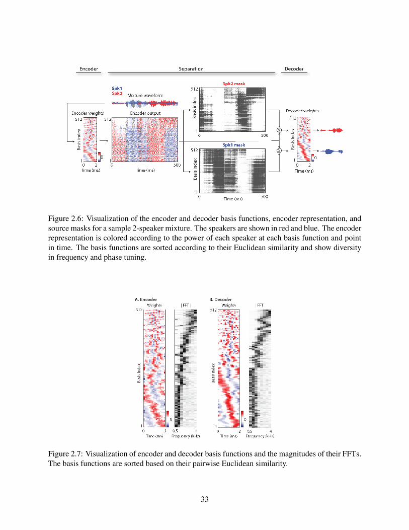
Figure 2.6: Visualization of the encoder and decoder basis functions, encoder representation, andsource masks for a sample 2-speaker mixture. The speakers are shown in red and blue. The encoderrepresentation is colored according to the power of each speaker at each basis function and pointin time. The basis functions are sorted according to their Euclidean similarity and show diversityin frequency and phase tuning.

Figure 2.7: Visualization of encoder and decoder basis functions and the magnitudes of their FFTs.The basis functions are sorted based on their pairwise Euclidean similarity.

33

2.3 DPRNN-TasNet: Stronger Long Sequence Modeling Ability

Conv-TasNet showed that improved separation performance can be achieved by using smaller

window size L. However, a smaller window comes at the cost of a significantly longer mixture

hidden representation [234], [243]. This poses an additional challenge as the sequential modeling

networks in LSTM-TasNet and Conv-TasNet might both have difficulties on learning such long-

term temporal dependency [196]. Moreover, unlike RNNs that have dynamic receptive fields,

TCNs with fixed receptive fields that are smaller than the sequence length are not able to fully

utilize the sequence-level dependency [179].

Dual-path RNN (DPRNN) is introduced here to replace TCN and tackle the aforementioned

issue in long sequence modeling. DPRNN organizes any kinds of RNN layers to model long se-

quential inputs in a very simple way. The intuition is to split the input sequence into shorter chunks

and interleave two RNNs, an intra-chunk RNN and an inter-chunk RNN, for local and global mod-

eling, respectively. In a DPRNN block, the intra-chunk RNN first processes the local chunks

independently, and then the inter-chunk RNN aggregates the information from all the chunks to

perform utterance-level processing. For a sequential input of length T , DPRNN with chunk size

K and chunk hop size P contains S chunks, where K and S corresponds to the input lengths for

the inter- and intra-chunk RNNs, respectively. When K ≈ S, the two RNNs have a sublinear

input length (O(√T )) as opposed to the original input length (O(T )), which greatly decreases the

optimization difficulty that arises when T is extremely large.

2.3.1 Modifications upon Conv-TasNet

The only difference between DPRNN-TasNet and Conv-TasNet is the use of DPRNN instead

of TCN. A DPRNN consists of three stages: segmentation, block processing, and overlap-add.

The segmentation stage splits a sequential input into overlapped chunks and concatenates all the

chunks into a 3-D tensor. The tensor is then passed to stacked DPRNN blocks to iteratively apply

local (intra-chunk) and global (inter-chunk) modeling in an alternate fashion. The output from the

34

last layer is transformed back to a sequential output with overlap-add method. Figure 2.8 shows

the flowchart of a DPRNN block.

Sequentialinput

...

�

�

�

�

�

��

2�

Bi-RNN

LayerNorm

(Bi-)RNN

FC FC

Overlap-Add Sequentialoutput

�

�

A.Segmentation B.DPRNNblock

C.Overlap-Add

LayerNorm

+ +

Figure 2.8: System flowchart of dual-path RNN (DPRNN). (A) The segmentation stage splits asequential input into chunks with or without overlaps and concatenates them to form a 3-D tensor.In the implementation, the overlap ratio is set to 50%. (B) Each DPRNN block consists of twoRNNs that have recurrent connections in different dimensions. The intra-chunk bi-directionalRNN is first applied to individual chunks in parallel to process local information. The inter-chunkRNN is then applied across the chunks to capture global dependency. Multiple blocks can bestacked to increase the total depth of the network. (C) The 3-D output of the last DPRNN block isconverted back to a sequential output by performing overlap-add on the chunks.

For a sequential input W ∈ RN×T where N is the feature dimension and T is the number of

time steps, the segmentation stage splits W into chunks of length K and hop size P . The first and

last chunks are zero-padded so that every sample in W appears and only appears in K/P chunks,

generating S equal size chunks Ds ∈ RN×K , s = 1, . . . , S. All chunks are then concatenated

together to form a 3-D tensor T = [D1, . . . ,DS] ∈ RN×K×S .

The segmentation output T is then passed to the stack of B DPRNN blocks. Each block

transforms an input 3-D tensor into another tensor with the same shape. Denote the input tensor

for block b = 1, . . . , B as Tb ∈ RN×K×S , where T1 = T. Each block contains two sub-modules

corresponding to intra- and inter-chunk processing, respectively. The intra-chunk RNN is always

bi-directional and is applied to the second dimension of Tb, i.e., within each of the S blocks:

Ub = [fb(Tb[:, :, i]), i = 1, . . . , S] (2.18)

where Ub ∈ RH×K×S is the output of the RNN, fb(·) is the mapping function defined by the RNN,

and Tb[:, :, i] ∈ RN×K is the sequence defined by chunk i. A linear fully-connected (FC) layer is

35

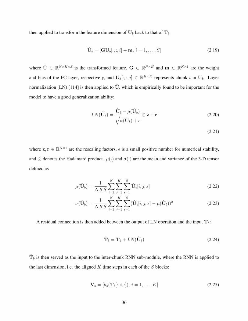
then applied to transform the feature dimension of Ub back to that of Tb

Ub = [GUb[:, :, i] + m, i = 1, . . . , S] (2.19)

where U ∈ RN×K×S is the transformed feature, G ∈ RN×H and m ∈ RN×1 are the weight

and bias of the FC layer, respectively, and Ub[:, :, i] ∈ RH×K represents chunk i in Ub. Layer

normalization (LN) [114] is then applied to U, which is empirically found to be important for the

model to have a good generalization ability:

LN(Ub) =Ub − µ(Ub)√σ(Ub) + ε

� z + r (2.20)

(2.21)

where z, r ∈ RN×1 are the rescaling factors, ε is a small positive number for numerical stability,

and � denotes the Hadamard product. µ(·) and σ(·) are the mean and variance of the 3-D tensor

defined as

µ(Ub) =1

NKS

N∑i=1

K∑j=1

S∑s=1

Ub[i, j, s] (2.22)

σ(Ub) =1

NKS

N∑i=1

K∑j=1

S∑s=1

(Ub[i, j, s]− µ(Ub))2 (2.23)

A residual connection is then added between the output of LN operation and the input Tb:

Tb = Tb + LN(Ub) (2.24)

Tb is then served as the input to the inter-chunk RNN sub-module, where the RNN is applied to

the last dimension, i.e. the aligned K time steps in each of the S blocks:

Vb = [hb(Tb[:, i, :]), i = 1, . . . , K] (2.25)

36

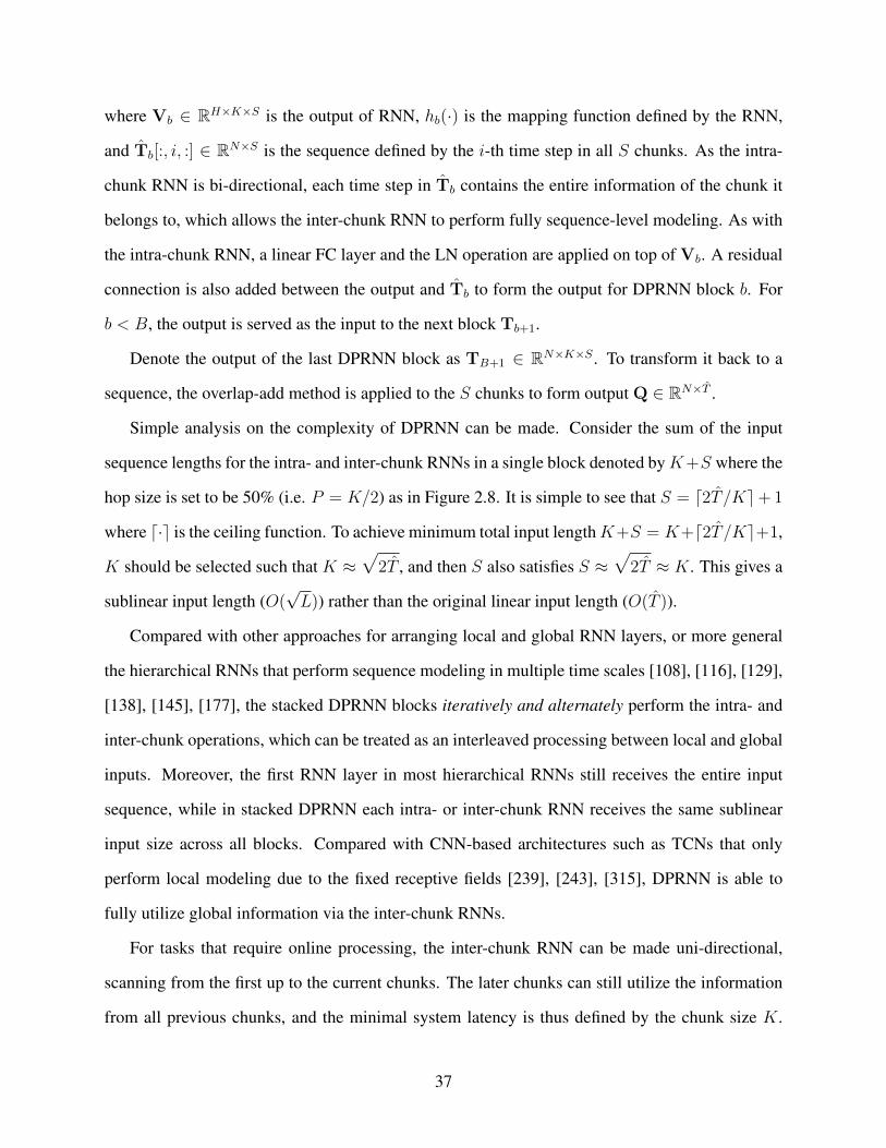
where Vb ∈ RH×K×S is the output of RNN, hb(·) is the mapping function defined by the RNN,

and Tb[:, i, :] ∈ RN×S is the sequence defined by the i-th time step in all S chunks. As the intra-

chunk RNN is bi-directional, each time step in Tb contains the entire information of the chunk it

belongs to, which allows the inter-chunk RNN to perform fully sequence-level modeling. As with

the intra-chunk RNN, a linear FC layer and the LN operation are applied on top of Vb. A residual

connection is also added between the output and Tb to form the output for DPRNN block b. For

b < B, the output is served as the input to the next block Tb+1.

Denote the output of the last DPRNN block as TB+1 ∈ RN×K×S . To transform it back to a

sequence, the overlap-add method is applied to the S chunks to form output Q ∈ RN×T .

Simple analysis on the complexity of DPRNN can be made. Consider the sum of the input

sequence lengths for the intra- and inter-chunk RNNs in a single block denoted byK+S where the

hop size is set to be 50% (i.e. P = K/2) as in Figure 2.8. It is simple to see that S = d2T /Ke+ 1

where d·e is the ceiling function. To achieve minimum total input lengthK+S = K+d2T /Ke+1,

K should be selected such that K ≈√

2T , and then S also satisfies S ≈√

2T ≈ K. This gives a

sublinear input length (O(√L)) rather than the original linear input length (O(T )).

Compared with other approaches for arranging local and global RNN layers, or more general

the hierarchical RNNs that perform sequence modeling in multiple time scales [108], [116], [129],

[138], [145], [177], the stacked DPRNN blocks iteratively and alternately perform the intra- and

inter-chunk operations, which can be treated as an interleaved processing between local and global

inputs. Moreover, the first RNN layer in most hierarchical RNNs still receives the entire input

sequence, while in stacked DPRNN each intra- or inter-chunk RNN receives the same sublinear

input size across all blocks. Compared with CNN-based architectures such as TCNs that only

perform local modeling due to the fixed receptive fields [239], [243], [315], DPRNN is able to

fully utilize global information via the inter-chunk RNNs.

For tasks that require online processing, the inter-chunk RNN can be made uni-directional,

scanning from the first up to the current chunks. The later chunks can still utilize the information

from all previous chunks, and the minimal system latency is thus defined by the chunk size K.

37

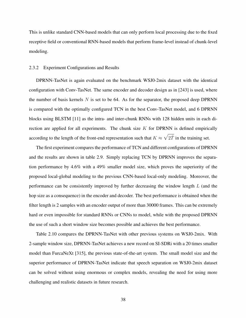
This is unlike standard CNN-based models that can only perform local processing due to the fixed

receptive field or conventional RNN-based models that perform frame-level instead of chunk-level

modeling.


DPRNN-TasNet is again evaluated on the benchmark WSJ0-2mix dataset with the identical

configuration with Conv-TasNet. The same encoder and decoder design as in [243] is used, where

the number of basis kernels N is set to be 64. As for the separator, the proposed deep DPRNN

is compared with the optimally configured TCN in the best Conv-TasNet model, and 6 DPRNN

blocks using BLSTM [11] as the intra- and inter-chunk RNNs with 128 hidden units in each di-

rection are applied for all experiments. The chunk size K for DPRNN is defined empirically

according to the length of the front-end representation such that K ≈√

2T in the training set.

The first experiment compares the performance of TCN and different configurations of DPRNN

and the results are shown in table 2.9. Simply replacing TCN by DPRNN improves the separa-

tion performance by 4.6% with a 49% smaller model size, which proves the superiority of the

proposed local-global modeling to the previous CNN-based local-only modeling. Moreover, the

performance can be consistently improved by further decreasing the window length L (and the

hop size as a consequence) in the encoder and decoder. The best performance is obtained when the

filter length is 2 samples with an encoder output of more than 30000 frames. This can be extremely

hard or even impossible for standard RNNs or CNNs to model, while with the proposed DPRNN

the use of such a short window size becomes possible and achieves the best performance.

Table 2.10 compares the DPRNN-TasNet with other previous systems on WSJ0-2mix. With

2-sample window size, DPRNN-TasNet achieves a new record on SI-SDRi with a 20 times smaller

model than FurcaNeXt [315], the previous state-of-the-art system. The small model size and the

superior performance of DPRNN-TasNet indicate that speech separation on WSJ0-2mix dataset

can be solved without using enormous or complex models, revealing the need for using more

challenging and realistic datasets in future research.

38

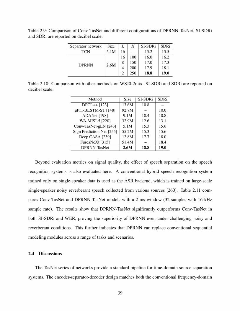
Table 2.9: Comparison of Conv-TasNet and different configurations of DPRNN-TasNet. SI-SDRiand SDRi are reported on decibel scale.

Separator network Size L K SI-SDRi SDRiTCN 5.1M 16 – 15.2 15.5

DPRNN 2.6M

16 100 16.0 16.28 150 17.0 17.34 200 17.9 18.12 250 18.8 19.0

Table 2.10: Comparison with other methods on WSJ0-2mix. SI-SDRi and SDRi are reported ondecibel scale.

Method Size SI-SDRi SDRiDPCL++ [123] 13.6M 10.8 –

uPIT-BLSTM-ST [148] 92.7M – 10.0ADANet [198] 9.1M 10.4 10.8

WA-MISI-5 [220] 32.9M 12.6 13.1Conv-TasNet-gLN [243] 5.1M 15.3 15.6Sign Prediction Net [255] 55.2M 15.3 15.6

Deep CASA [239] 12.8M 17.7 18.0FurcaNeXt [315] 51.4M – 18.4DPRNN-TasNet 2.6M 18.8 19.0

Beyond evaluation metrics on signal quality, the effect of speech separation on the speech

recognition systems is also evaluated here. A conventional hybrid speech recognition system

trained only on single-speaker data is used as the ASR backend, which is trained on large-scale

single-speaker noisy reverberant speech collected from various sources [260]. Table 2.11 com-

pares Conv-TasNet and DPRNN-TasNet models with a 2-ms window (32 samples with 16 kHz

sample rate). The results show that DPRNN-TasNet significantly outperforms Conv-TasNet in

both SI-SDRi and WER, proving the superiority of DPRNN even under challenging noisy and

reverberant conditions. This further indicates that DPRNN can replace conventional sequential

modeling modules across a range of tasks and scenarios.

2.4 Discussions

The TasNet series of networks provide a standard pipeline for time-domain source separation

systems. The encoder-separator-decoder design matches both the conventional frequency-domain

39

Table 2.11: SI-SDRi and WER results for noisy reverberant separation and recognition task. Win-dow size is set to 32 samples for both models, and the chunk size is set to 100 frames for DPRNN-TasNet. WER is calculated for both separated speakers.

Separator network Size SI-SDRi WERTCN 5.1M 7.6 28.7

DPRNN 2.6M 8.4 25.9%Noise-free reverberant speech – – 9.1%

systems and the newly proposed time-domain systems, where the difference mainly lies on the

operation selected in the encoder and decoder. Frequency-domain systems can also be trained with

time-domain training objectives to form an end-to-end pipeline by treating STFT and its inverse as

encoder and decoder and backpropagating together with the separator.

TasNet, as well as its extensions, can be applied to the separation of a wide range of nonspeech

signals. For example, TasNet has been applied to the separation of vocal and instrumental tracks,

seismic signals [297], electrocardiograms signals, and environmental sounds. The successful ap-

plications of TasNet on these topics show that advances in speech separation models have great

potential to reform the development of source separation systems in other domains and eventually

towards a universal source separation system.

40

Chapter 3: Multi-channel System: Filter-and-sum Network

In this chapter I will introduce a time-domain multi-channel system, the filter-and-sum network

(FaSNet), for multi-channel source separation. The concept of neural beamformers has been dis-

cussed and reviewed in Chapter 1.2, where a neural network is used to enhance the spatial filtering

process or even directly learn the spatial filters. The intuition of FaSNet is to replace the frequency-

domain spatial filtering process with a time-domain process, where the time-domain spatial filters

are directly learned by a neural network. However, there are two main differences compared with

the frequency-domain beamformers: first, FaSNet performs adaptive filter-and-sum beamforming

at frame-level, while conventional frequency-domain neural beamformers perform utterance-level

beamforming; second, FaSNet moves all the operations to time domain.

According to how the filter-and-sum operation is defined and how the filters are estimated,

three versions of FaSNet have been proposed: the two-stage FaSNet [241] was the first version of

FaSNet that performed a two-stage spatial filtering process in time domani, the TAC-FaSNet [286]

was the second version that achieved full invariance to microphone array configurations, which

was specially designed for ad-hoc array applications; the iFaSNet [289] was the third version of

FaSNet that defined the filter-and-sum operation in a hidden representation space instead of the

waveforms with improved cross-channel feature extraction.

3.1 Two-stage FaSNet: Time-domain Adaptive Beamforming

Prior to the two-stage FaSNet, all neural beamformers were applied in frequency domain with

an explicit formulation of a selected beamformer, e.g., MVDR or GEV beamformer. The two-stage

FaSNet performs end-to-end time-domain adaptive beamforming with two stages: the first stage

selects a reference microphone and estimates its beamforming filters for all the target sources, and

41

the second stage utilizes the outputs from the first stage to estimate the beamforming filters for

the remaining channels. The outputs from the first and second stages are summed to generate

the final separation outputs. Intuitively, the first stage in the two-stage FaSNet can be treated as

a pre-separation single-channel separation process with additional cross-channel features, and the

second stage can be viewed as a target speaker extraction process with each of the separated outputs

in the first stage.

3.1.1 System Pipeline

The problem of frame-level time-domain filter-and-sum beamforming is defined as estimating a

set of time-domain filters for a microphone array of N ≥ 2 microphones, such that the summation

of the filtered signals of all microphones provides the best estimation of a signal of interest in a

selected reference microphone. The signals xi are first split at each microphone into frames of L

samples with a hop size of H ∈ [0, L− 1] samples

xit = xi[tH : tH + L− 1], t ∈ Z, i = 1, . . . , N (3.1)

where t is the frame index, i is the index of the microphone and the operation x[a : b] selects the

values of vector x from index a to index b. To account for the time-difference of arrival (TDOA) of

the signal of interest at different microphones, the filter-and-sum operation is applied on a context

window around frame t for each microphone to generate the beamformed output at frame t

yt =N∑i=1

hit ~ xit (3.2)

where yt ∈ R1×L is the beamformed signal at frame t, xit = xi[tH − W : tH + 2W − 1] ∈

R1×(L+2W ) is the context window around xt for microphone i, hit ∈ R1×(2W+1) is the beamforming

filter to be learned for microphone i, and ~ represents the convolution operation. For frames where

tH < W or tH + 2W > l where l is the total length of the signal, zero is padded to the context

windows. The use of context window xit is to make sure the model can capture cross-microphone

42

delays of ±W samples, since the directions of the sources are always unknown. As shown in

[125], the use of the context window incorporates the estimation of cross-microphone delay into

the learning process of hit. The problem of filter-and-sum beamforming thus becomes estimating

hit given the observations of xi. For simplicity, the frame index t is dropped in the following

discussions where there is no ambiguity.

The first stage is to calculate the beamforming filter for the reference microphone which

is randomly selected from the array. Motivated by the GCC-PHAT feature [2], [10] in other

frequency-domain beamformers and tasks such as DOA and TDOA estimation, a frame-level nor-

malized cross-correlation (NCC) is calculated as the inter-channel feature. To be specific, let

x1 ∈ R1×(L+2W ) be the context window of the signal in the reference microphone, and xi ∈

R1×L, i = 2, . . . , N be the corresponding center frame of all the other microphones with same

index, then the NCC feature, which is defined as the cosine similarity here, is calculated between

x1 and xi: x1j = x1[j : j + L− 1]

f ij =x1j (xi)T

‖x1j‖2‖xi‖2

, j = 1, . . . , 2W + 1 (3.3)

where f i ∈ R1×(2W+1) is the cosine similarity between reference microphone and microphone i.

The NCC feature contains both the TDOA information and the content-dependent information of

the signal of interest in the reference microphone and the other microphones. In order to combine

the N − 1 such features f i, i = 2, . . . , N for all non-reference microphones in a permutation-free

manner (i.e. independent from microphone indexes), a mean-pooling operation is applied:

fi

=1

N − 1

N∑i=2

f i (3.4)

For channel-specific feature, a linear layer is applied on x1 ∈ R1×L, the center frame of x1, to

43

create a K-dimensional embedding R1 ∈ R1×K

R1 = x1U (3.5)

where U ∈ RL×K is the weight matrix. R1 is then concatenated with fi and passed to a separation

module to generate C beamforming filters h1c ∈ R1×(2W+1), c = 1, . . . , C where C is the number

of sources of interest:

{h1c}Cc=1 = H1

([R1, f ]

)(3.6)

where H1(·) is the mapping function defined by the separation module. h1c is then convolved with

x1 to generate the beamformed output of source c, y1c ∈ R1×L, for the reference microphone:

y1c = x1 ~ h1

c . (3.7)

The second stage is to estimate the beamforming filters hic, i = 2, . . . , N for all remaining

microphones. Using the output of each estimated sources of interest from the first stage y1c as the

cue, a similar procedure as above is applied to all the remaining microphones. For microphone i

with context window xi ∈ R1×(L+2W ), the NCC feature is calculated between it and y1c :

xij = xi[j : j + L− 1]

gic,j =xij(y1

c)T

‖xij‖2‖y1

c‖2

, j = 1, . . . , 2W + 1 (3.8)

An filter extraction module with its corresponding mapping function H2(·) is then used to

generate hic given gic ∈ R1×(2W+1) and the linear transformation Ri = xiU:

hic = H2

([Ri,gic]

)(3.9)

Note that all remaining microphones share the same extraction module for each of the target

44

sources. The filters hic are then convolved with xi and summed up to y1c to generate the final

beamformed output of source c

yc = y1c +

N∑i=2

xi ~ hic (3.10)

Finally, all segments in yc are transformed back to the full utterance y∗c ∈ R1×L through the

overlap-and-add operation.

The output of the two-stage FaSNet can also be passed to any single-channel enhancement sys-

tem for further performance improvement. As FaSNet directly generates waveforms, the tandem

system can still be trained end-to-end for either time-domain or frequency-domain objectives.

Similar to the TasNet models, the training objective of FaSNet can still be the negative SI-SDR

score under the PIT framework. For tasks where frequency-domain output is favored (e.g., ASR

tasks), mel-spectrogram with scale-invariant MSE (SI-MSE) loss is used as the training objective:

Yc =

∣∣∣∣STFT(

yc‖yc‖2

)∣∣∣∣Y∗c =

∣∣∣∣STFT(

y∗c‖y∗c‖2

)∣∣∣∣ (3.11)

LSI-MSE =1

C

C∑c=1

||YcM−Y∗cM||22 (3.12)

where Yc,Y∗c ∈ RT×F are the magnitude spectrograms of the target and estimated signals respec-

tively, and M ∈ RF×D is the mel-filterbank.

3.1.2 Design of Filter Separation and Extraction Modules

The filter separation module in the first stage and the filter extraction module in the second stage

are both TCN models proposed in the Conv-TasNet model in Chapter 2.2.1. The main difference

with the TCN applied for Conv-TasNet is the design of the output layer. Suppose that {p1c}Cc=1 ∈

R1×K denote the outputs of the last TCN block at the first stage and serve as the input to the output

45

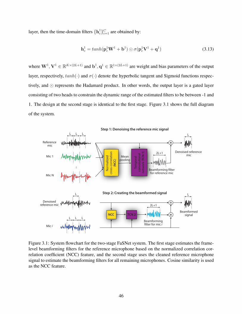
layer, then the time-domain filters {h1c}Cc=1 are obtained by:

h1c = tanh(p1

cW1 + b1)� σ(p1

cV1 + q1) (3.13)

where W1,V1 ∈ RK×(2L+1) and b1,q1 ∈ R1×(2L+1) are weight and bias parameters of the output

layer, respectively, tanh(·) and σ(·) denote the hyperbolic tangent and Sigmoid functions respec-

tively, and � represents the Hadamard product. In other words, the output layer is a gated layer

consisting of two heads to constrain the dynamic range of the estimated filters to be between -1 and

1. The design at the second stage is identical to the first stage. Figure 3.1 shows the full diagram

of the system.

...

L

Reference mic

Mic 1

Mic N

Nor

mal

ized

cr

oss-

corr

elat

ion

(NCC

)

Meanpooling

Tem

pora

l co

nvol

utio

nal

netw

ork

(TCN

1)

2L+1

Beamforming �lterfor reference mic

*

L

Denoised reference mic

Denoisedreference mic

Mic i

NCC TCN 2

2L+1

Beamforming�lter for mic i

+

L

Beamformedsignal

L

*

Step 1: Denoising the reference mic signal

Step 2: Creating the beamformed signal

Decoder

L

... ... ... ...Encoder ×

Mixturewaveform

Separatedwaveforms

L

Separation

LL

L LL

Deep vocoder

Encoder &separator

Single sourceencoder i

Iteration 1:

Iterations i = 2, ..., k:

X Y1c

Latent representationof source C, iteration i

Separated waveform of source C, iteration i

S 1c

^

S i-1c

^ Deep vocoderY i-1

c S ic

^

Input waveform

Figure 3.1: System flowchart for the two-stage FaSNet system. The first stage estimates the frame-level beamforming filters for the reference microphone based on the normalized correlation cor-relation coefficient (NCC) feature, and the second stage uses the cleaned reference microphonesignal to estimate the beamforming filters for all remaining microphones. Cosine similarity is usedas the NCC feature.

46


The evaluation of the two-stage FaSNet is applied on three tasks:

1. Echoic noisy speech enhancement (ESE): Speech denoising and dereverberation are jointly

performed in an echoic environment;

2. Echoic noisy speech separation (ESS): The direct path of two speakers are separated in a

noisy, echoic environment;

3. Multichannel noisy ASR: The 3rd CHiME challenge dataset [95] is selected for ASR task.

The direct-path speech signals for all sources of interest are always used as the target, which means

that the system attempts to perform joint denoising/separation and dereverberation.

For ESE and ESS tasks, simulated datasets are generated from a circular omni-directional

microphone array with a maximum of 4 microphones evenly distributed. The diameter of the

array is fixed to 10 cm. The positions of the sources (speakers and the noise) and the center of

the microphone array are randomly sampled, with the constraint that all sources should be at least

0.5 m away from the room walls. The height for all sources is fixed to 1 m. The room impluse

response (RIR) filters are then simulated with the image method [3], and specifically with the

gpuRIR toolbox [270]. The length and the width of the rooms are randomly sampled within the

range [3, 8] m with a fixed height of 3 m. The utterances in the datasets are sampled from the TIMIT

dataset [8]. Each speaker’s utterances are splitted into 7 training, 2 validation and 1 test samples,

and then the training, validation and test sets are generated within the corresponding categories to

include 20000, 5000 and 3000 rooms respectively. Each room contains two speakers and one noise

source, within which the noise is randomly sampled from first 80 samples in the 100 Nonspeech

Corpus [334] for training and validation sets and all 100 samples for the test set. For ESE, the

relative SNR between the speaker and the noise is randomly sampled between [−5, 15] dB. In

ESS, the relative SNR between the two speakers is randomly sampled between [−5, 5] dB and the

noise is randomly sampled between [−5, 15] dB with respect to the low energy speaker.

47

Table 3.1 shows the symbols for the hyperparameters in the two-stage FaSNet. Each TCN

has an identical design to [201] and contains R repeats of the 1-D convolutional blocks with P

blocks in each repeat, where R = 2 and P = 5 are used in all experiments. The size of the 1-D

convolutional kernel in each 1-D convolutional block is 3, and the input and hidden channels in

each block are set to 64 and 320, respectively. The embedding dimension K is set to 64. The

number of parameters in each TCN is thus 0.76M. For tandem systems with a single-channel

system for post-enhancement, the Conv-TasNet configuration [201] is adopted but the masking

layer is modified into a direct regression layer. The model size of the single-output Conv-TasNet

is 1.9M. The window size L and context size W are identical in all experiments.

Table 3.1: Hyperparameters in two-stage FaSNet.

Symbol DescriptionL Window size (in samples)P Number of convolutional blocks in each repeat in TCNR Number of repeats in TCNK Dimension of embeddings as well as the output of TCN

In the ASR and ESE tasks, each TCN estimates one beamforming filter at each frame, while in

the ESS task, each TCN estimates two beamforming filters corresponding to the two speakers.

In order to show the advantages and performance of the two-stage FaSNet, the model is com-

pared against a variety of classical beamformers. Both beamformers in the time- and frequency-

domain are considered. The comparison on the time-domain beamformers is carried out since it

represents a fairer comparison to FaSNet which is also based on the time domain. This comparison

is extended to more traditional and more robust frequency-domain beamformers which are vastly

used in practice. Four classes of beamformers are considered in the comparison. The first class

is time-domain (TD) beamformers and comprises time-domain multi-channel Wiener filter (TD-

MWF) and time-domain minimum variance distortionless response (TD-MVDR) beamformers

[67]. The second class is frequency-domain (FD) beamformers and considers the speech distor-

tion weigted MWF (SDW-MWF) and FD-MVDR beamformers [52]. For both of these classes

the eigen-decomposition method is used in order to estimate the steering vector [57] from the

48

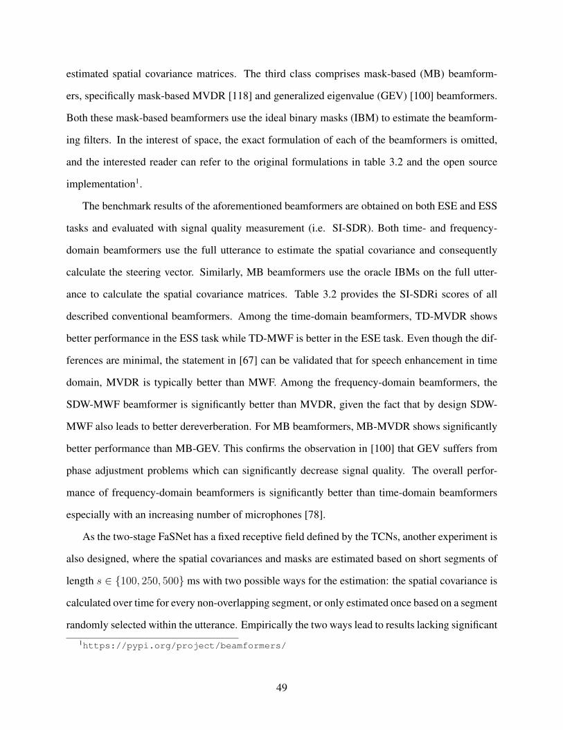
estimated spatial covariance matrices. The third class comprises mask-based (MB) beamform-

ers, specifically mask-based MVDR [118] and generalized eigenvalue (GEV) [100] beamformers.

Both these mask-based beamformers use the ideal binary masks (IBM) to estimate the beamform-

ing filters. In the interest of space, the exact formulation of each of the beamformers is omitted,

and the interested reader can refer to the original formulations in table 3.2 and the open source

implementation1.

The benchmark results of the aforementioned beamformers are obtained on both ESE and ESS

tasks and evaluated with signal quality measurement (i.e. SI-SDR). Both time- and frequency-

domain beamformers use the full utterance to estimate the spatial covariance and consequently

calculate the steering vector. Similarly, MB beamformers use the oracle IBMs on the full utter-

ance to calculate the spatial covariance matrices. Table 3.2 provides the SI-SDRi scores of all

described conventional beamformers. Among the time-domain beamformers, TD-MVDR shows

better performance in the ESS task while TD-MWF is better in the ESE task. Even though the dif-

ferences are minimal, the statement in [67] can be validated that for speech enhancement in time

domain, MVDR is typically better than MWF. Among the frequency-domain beamformers, the

SDW-MWF beamformer is significantly better than MVDR, given the fact that by design SDW-

MWF also leads to better dereverberation. For MB beamformers, MB-MVDR shows significantly

better performance than MB-GEV. This confirms the observation in [100] that GEV suffers from

phase adjustment problems which can significantly decrease signal quality. The overall perfor-

mance of frequency-domain beamformers is significantly better than time-domain beamformers

especially with an increasing number of microphones [78].

As the two-stage FaSNet has a fixed receptive field defined by the TCNs, another experiment is

also designed, where the spatial covariances and masks are estimated based on short segments of

length s ∈ {100, 250, 500} ms with two possible ways for the estimation: the spatial covariance is

calculated over time for every non-overlapping segment, or only estimated once based on a segment

randomly selected within the utterance. Empirically the two ways lead to results lacking significant

1https://pypi.org/project/beamformers/

49

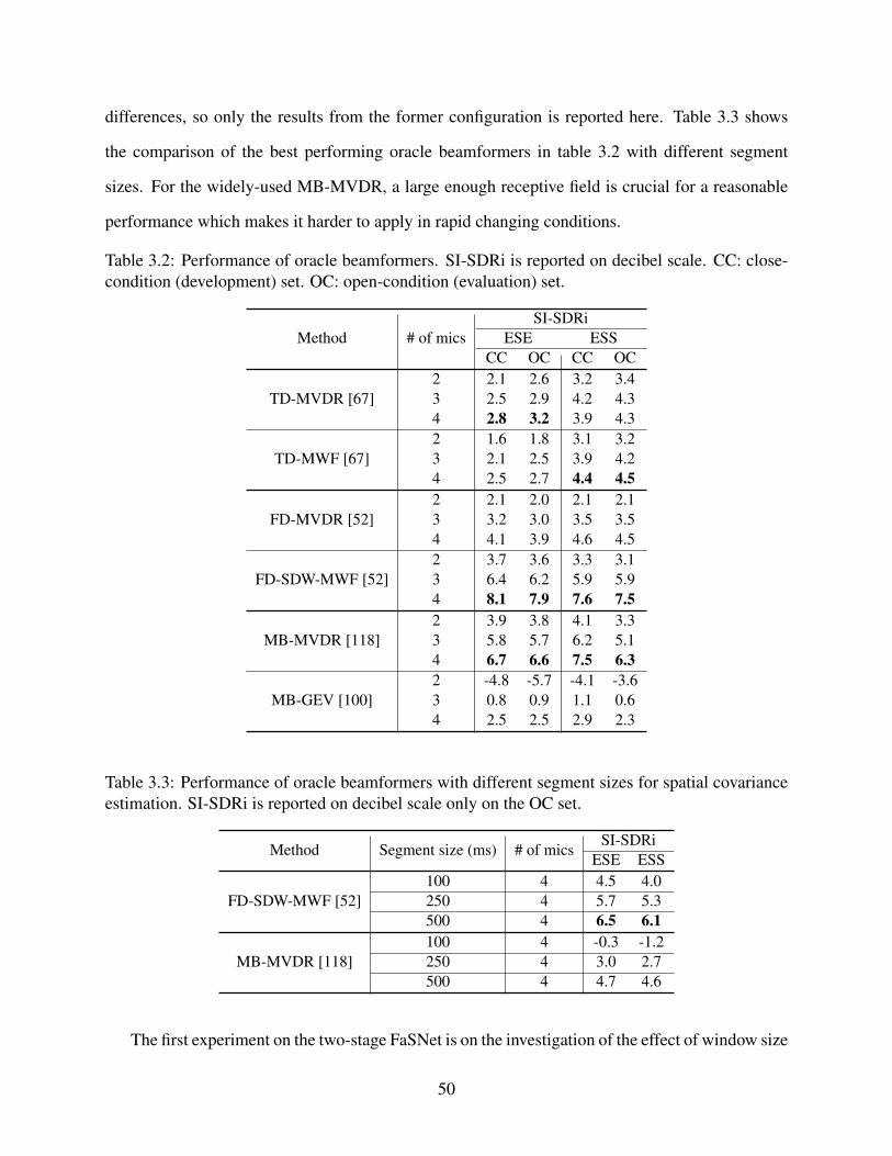
https://pypi.org/project/beamformers/

differences, so only the results from the former configuration is reported here. Table 3.3 shows

the comparison of the best performing oracle beamformers in table 3.2 with different segment

sizes. For the widely-used MB-MVDR, a large enough receptive field is crucial for a reasonable

performance which makes it harder to apply in rapid changing conditions.

Table 3.2: Performance of oracle beamformers. SI-SDRi is reported on decibel scale. CC: close-condition (development) set. OC: open-condition (evaluation) set.

Method # of micsSI-SDRi

ESE ESSCC OC CC OC

TD-MVDR [67]2 2.1 2.6 3.2 3.43 2.5 2.9 4.2 4.34 2.8 3.2 3.9 4.3

TD-MWF [67]2 1.6 1.8 3.1 3.23 2.1 2.5 3.9 4.24 2.5 2.7 4.4 4.5

FD-MVDR [52]2 2.1 2.0 2.1 2.13 3.2 3.0 3.5 3.54 4.1 3.9 4.6 4.5

FD-SDW-MWF [52]2 3.7 3.6 3.3 3.13 6.4 6.2 5.9 5.94 8.1 7.9 7.6 7.5

MB-MVDR [118]2 3.9 3.8 4.1 3.33 5.8 5.7 6.2 5.14 6.7 6.6 7.5 6.3

MB-GEV [100]2 -4.8 -5.7 -4.1 -3.63 0.8 0.9 1.1 0.64 2.5 2.5 2.9 2.3

Table 3.3: Performance of oracle beamformers with different segment sizes for spatial covarianceestimation. SI-SDRi is reported on decibel scale only on the OC set.

Method Segment size (ms) # of micsSI-SDRi

ESE ESS

FD-SDW-MWF [52]100 4 4.5 4.0250 4 5.7 5.3500 4 6.5 6.1

MB-MVDR [118]100 4 -0.3 -1.2250 4 3.0 2.7500 4 4.7 4.6

The first experiment on the two-stage FaSNet is on the investigation of the effect of window size

50

L. Table 3.4 shows how different frame sizes affect the system performance. It can be observed that

a longer window size leads to constantly better performance, which is expected as higher frequency

resolution can be achieved. As the system latency of the two-stage FaSNet is 2L, tradeoff between

performance and window size needs to be considered for applications that strictly require low-

latency processing. Here the best performing system, i.e. L = 16, is selected for all following

experiments.

Table 3.4: Dependence of SI-SDRi on frame size for a 2-ch two-stage FaSNet in the ESE task.

L2 4 8 16

CC 1.6 2.4 3.3 4.0OC 1.4 2.2 3.0 3.7

The second experiment compares the two-stage FaSNet with Conv-TasNet [201], the single-

channel separation model, as they share a same design on the separation modules. Table 3.5

provides the comparison across different number of microphones and causality settings. It can be

observed that in a noncausal setting, the two-stage FaSNet achieves on par performance with the

single-channel Conv-TasNet baseline of 4 microphones, while in a causal setting, it outperforms

Conv-TasNet even with only 2 microphones. Moreover, adding a post single-channel enhancement

network constantly improves the performance across almost all configurations on both tasks. The

4-channel tandem system is able to achieve on par performance with an MB-MVDR system with

oracle IBM, and is significantly better than the segment-level oracle MB-MVDR. This shows that

when comparing with frequency-domain beamformers which highly rely on a long segment for

robust spatial covariance estimation, the two-stage FaSNet has better potential for low-latency

processing on much shorter segments.

The third experiment evaluates the two-stage FaSNet on CHiME-3 dataset to investigate its

potential as the front-end for speech recognition systems. Table 3.6 shows the performance of the

two-stage FaSNet with respect to signal quality measure. Two different training targets, the rever-

berant clean signal or the original clean signal, are applied during training. Note that the original

clean source has an unknown shift with the oracle direct path signal in the reference microphone,

51

Table 3.5: Performance of two-stage FaSNet and tandem system in both ESE and ESS tasks.

Method Size Causal # of micsSI-SDRi

ESE ESSCC OC CC OC

Conv-TasNet 1.9M×

15.3 5.0 4.1 4.1

X 3.5 3.3 2.7 2.6

FaSNet 1.5M

×2 4.0 3.7 3.7 3.63 4.4 4.1 4.0 3.94 5.3 5.0 4.7 4.6

X2 3.8 3.5 3.2 3.13 4.1 3.8 3.5 3.44 4.5 4.3 3.9 3.8

Tandem 3.4M

×2 5.8 5.5 4.5 4.43 5.4 5.0 5.5 5.54 6.7 6.4 6.2 6.1

X2 4.8 4.5 3.9 3.83 5.3 5.0 4.1 4.04 4.7 4.4 4.5 4.4

so here a shift invariant training (SIT) strategy is applied, where the maximum SI-SNR between

the system output and the original clean signal with ±2 ms of shift is seleted for backpropagation.

The results show that the two-stage FaSNet is significantly better than the Conv-TasNet baseline

with both targets, further proving its effectiveness on real-world recordings. Table 3.7 compares

the word error rate (WER) of the two-stage FaSNet and the official CHiME-3 baseline system

on the recognition task. The officially provided DNN baseline recognizer is used as the backend

ASR system, although more advanced systems with fully end-to-end training may further boost the

performance. The table shows that when training with the original clean source as target and SI-

SNR as objective, the two-stage FaSNet is able to achieve 9.3% relative WER reduction (RWERR)

compared with the MVDR baseline, and when training with the mel-spectrogram of the original

clean signal as target with SI-MSE as objective, the two-stage FaSNet achieves a 14.3% RWERR.

This result proves that when training with a frequency-domain objective that favors ASR backends,

two-stage FaSNet can also serve as an effective ASR front-end.

Finally, to better understand the beampatterns of the estimated time-domain filters, figure 3.2

visualizes them for two example utterances in the ESS task. The figure shows the beampatterns

52

Table 3.6: Performance of two-stage FaSNet on CHiME-3 evaluation dataset. SI-SDRi is reportedon decibel scale.

Target Method Causal SI-SDRi

Reverberant cleanConv-TasNet × 8.7

FaSNet× 12.2X 10.6

Clean sourceConv-TasNet × 7.5

FaSNet× 11.6X 11.1

Table 3.7: Performance of two-stage FaSNet on CHiME-3 evaluation dataset of real recordings.WER is reported.

Method Target WER (%)Noisy - 32.53

Baseline - 32.48

FaSNetReverberant clean 32.23

Clean source 29.47Mel-spectrogram 27.89

estimated by the model at different frames of the utterances. The beampatterns are shown as a func-

tion of frequency and DOA. The two-stage FasNet learns specific beampatterns which are content-

dependent within each utterance, where different regions have different beampatterns. Specifically,

nonspeech regions receive filters with null pattern for both utterances, further proving the adapta-

tion ability of FaSNet across the utterance.

3.2 TAC-FaSNet: Microphone-number-invariant and Geometry-independent Processing

There are two core drawbacks in the two-stage FaSNet. First, the processing in the second stage

only makes use of the pairwise information of the output from the first stage and another remaining

channel, which prevents the system from utilizing the information from all microphones to make

a global decision during filter estimation. Second, failures in the first stage may greatly affect the

performance of the second stage. To allow the model to perform a single-stage filter estimation

while making use of the global information and being invariant to the microphone number and

permutation configurations, the transform-average-concatenate (TAC) is proposed to tackle the

53

0 0.5 1 1.5Time (s)

−0.002

0.000

0.002

0.004A

mpl

itud

e(a

u)

0 2 4 6 8Frequency (kHz)

0

45

90

135

180

DO

A(d

eg)



0.0 0.2 0.4 0.6 0.8 0 8 16 24 32 0 8 16 240 8 16 24

0 0.5 1 1.5Time (s)

−0.002

0.000

0.002

Am

plit

ude

(au)


0

45

90

135

180

DO

A(d

eg)



0.00 0.15 0.30 0.45 0 8 16 24 32 0 8 16 24 320 8 16 24 32

Figure 3.2: Beampattern examples for two different utterances in the ESS task.

disadvantages of the two-stage FaSNet.

A TAC module takes the feature from multiple channels as input. It first transforms each

channel’s feature with a sub-module shared by all channels, and then the outputs are averaged as a

global-pooling stage and passed to another sub-module for extra nonlinearity. The corresponding

output is then concatenated with each of the outputs of the first transformation sub-module and

passed to a third sub-module for generating channel-dependent outputs. It is easy to see that, with

54

parameter sharing at the transform and concatenate stages and the permutation-invariant property

of the average stage, TAC guarantees channel permutation and number invariant processing and is

always able to make global decisions.

3.2.1 Modifications upon the Two-stage FaSNet

There are three differences between the TAC-FaSNet and the two-stage FaSNet. First, the

TAC module is introduced and applied to ensure the microphone number and geometry invariant

property. Second, the two-stage design is replaced by a single-stage design to better utilize the

global information. Third, the TCN separation module is replaced by DPRNN blocks for better

sequential modeling ability.

To introduce the design of the TAC module, consider an N -channel microphone array with an

arbitrary geometry whereN ∈ {2, . . . , Nm} can vary between 2 and a pre-defined maximum num-

ber Nm ≥ 2. Each channel is represented by a sequential feature Zi ∈ RT×∗, i = 1, . . . , N where

T denotes the sequence length and ∗ denotes arbitrary feature dimensions. Only one-dimensional

features, i.e. Zi ∈ RT×K , are considered here for simplicity, although the proposed method can be

easily extended to higher dimensions.

A TAC module first transforms each channel’s feature with a shared sub-module. Although

any neural network architectures can be applied, here a simple fully-connected (FC) layer with

parametric rectified linear unit (PReLU) activation is applied at each time step:

f i,j = P (zi,j), j = 1, . . . , T (3.14)

where zi,j ∈ R1×K is the j-th time step in Zi, P (·) is the mapping function defined by the FC layer,

and f i,j ∈ R1×D denotes the output for channel i at time step j. All features f i,j, i = 1, . . . , N at

time step j are then averaged as a global-pooling stage, and passed to another FC layer with PReLU

55

activation:

f j = R(1

N

N∑i=1

f i,j) (3.15)

where R(·) is the mapping function defined by this FC layer and f j ∈ R1×D is the output at time

step j. f j is then concatenated with f i,j at each channel and passed to a third FC layer with PReLU

activation to generate channel-specific output gi,j ∈ R1×D:

gi,j = S([f i,j; f j]) (3.16)

where S(·) is the mapping function defined by this FC layer and [x; y] denotes the concatenation

operation of vector x and y. A residual connection is then added between the original input zi,j

and gi,j to form the output of the TAC module:

zi,j = zi,j + gi,j (3.17)

Figure 3.3 shows the flowchart of a TAC module.

Figure 3.3: Flowchart for the TAC module. A transform module is shared across all the channels totransform the input at each channel via a nonlinear mapping. An average module applies average-pooling across the channels and applies another nonlinear mapping. A concatenate module con-catenates the outputs from the transform and average stages and generates channel-dependentoutputs.

TAC is closely related to the recent progress in permutation invariant functions and functions

defined on sets [174]. Permutation invariant neural architectures have been widely investigated in

56

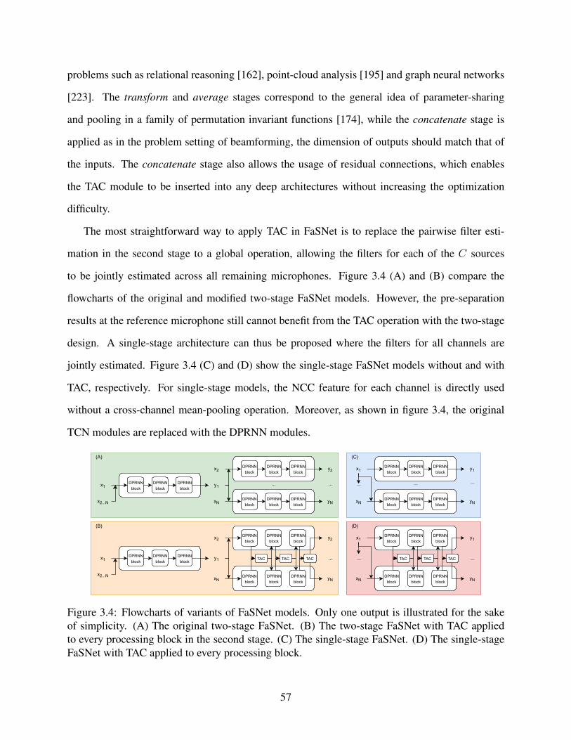
problems such as relational reasoning [162], point-cloud analysis [195] and graph neural networks

[223]. The transform and average stages correspond to the general idea of parameter-sharing

and pooling in a family of permutation invariant functions [174], while the concatenate stage is

applied as in the problem setting of beamforming, the dimension of outputs should match that of

the inputs. The concatenate stage also allows the usage of residual connections, which enables

the TAC module to be inserted into any deep architectures without increasing the optimization

difficulty.

The most straightforward way to apply TAC in FaSNet is to replace the pairwise filter esti-

mation in the second stage to a global operation, allowing the filters for each of the C sources

to be jointly estimated across all remaining microphones. Figure 3.4 (A) and (B) compare the

flowcharts of the original and modified two-stage FaSNet models. However, the pre-separation

results at the reference microphone still cannot benefit from the TAC operation with the two-stage

design. A single-stage architecture can thus be proposed where the filters for all channels are

jointly estimated. Figure 3.4 (C) and (D) show the single-stage FaSNet models without and with

TAC, respectively. For single-stage models, the NCC feature for each channel is directly used

without a cross-channel mean-pooling operation. Moreover, as shown in figure 3.4, the original

TCN modules are replaced with the DPRNN modules.10/22/2019 flowchart.drawio

1/1

DPRNNblock

DPRNNblock

DPRNNblock

x1 y1

DPRNNblock

DPRNNblock

DPRNNblock

x2...N

DPRNNblock

DPRNNblock

DPRNNblock

x2

xN

...

y2

yN

DPRNNblock

DPRNNblock

DPRNNblock

x1 y1

DPRNNblock

DPRNNblock

DPRNNblock

x2...N

DPRNNblock

DPRNNblock

DPRNNblock

x2

xN

y2

yN

TAC TAC TAC

...

...

DPRNNblock

DPRNNblock

DPRNNblock

DPRNNblock

DPRNNblock

DPRNNblock

x1

xN

... ...

y1

yN

...

DPRNNblock

DPRNNblock

DPRNNblock

DPRNNblock

DPRNNblock

DPRNNblock

x1

xN

y1

yN

TAC TAC TAC ......

(A)

(B)

(C)

(D)

Figure 3.4: Flowcharts of variants of FaSNet models. Only one output is illustrated for the sakeof simplicity. (A) The original two-stage FaSNet. (B) The two-stage FaSNet with TAC appliedto every processing block in the second stage. (C) The single-stage FaSNet. (D) The single-stageFaSNet with TAC applied to every processing block.

57


The two-stage FaSNet baseline and the TAC-FaSNet are evaluated on the task of multi-channel

two-speaker noisy speech separation with both ad-hoc and fixed geometry microphone arrays.

A multi-channel noisy reverberant dataset with 20000, 5000 and 3000 4-second long utterances is

simulated from the Librispeech dataset [109]. Two speakers and one nonspeech noise are randomly

selected from the 100-hour Librispeech dataset and the 100 Nonspeech Corpus [334], respectively.

An overlap ratio between the two speakers is uniformly sampled between 0% and 100% such

that the average overlap ratio across the dataset is 50%. The two speech signals are then shifted

accordingly and rescaled to a random relative SNR between 0 and 5 dB. The noise is repeated if

its length is smaller than 4 seconds, and the relative SNR between the power of the sum of the two

clean speech signals and the noise is randomly sampled between 10 and 20 dB. The transformed

signals are then convolved with RIRs generated by the image method [3] using the gpuRIR toolbox

[270]. The length and width of the room are randomly sampled between 3 and 10 meters, and the

height is randomly sampled between 2.5 and 4 meters. The reverberation time (T60) is randomly

sampled between 0.1 and 0.5 seconds. The echoic signals are summed to create the mixture for

each microphone. All microphone, speaker and noise locations in the ad-hoc array dataset are

randomly sampled to be at least 0.5 m away from the room walls. In the fixed geometry array

dataset, the microphone center is first sampled and then 6 microphones are evenly distributed

around a circle with diameter of 10 cm. The speaker locations are then sampled such that the

average speaker angle with respect to the microphone center is uniformly distributed between 0

and 180 degrees. The noise location is sampled without further constraints. The ad-hoc array

dataset contains utterances with 2 to 6 microphones, where the number of utterances for each

microphone configuration is set equal.

Single-channel baseline is also added here for a more comprehensive comparison. The first

stage in the two-stage FaSNet is used as a modification to the TasNet model, where the separation

is done by estimating filters for each context frame in the mixture instead of masking matrices

on a generated front-end. This model is referred to as TasNet-filter. For adding NCC features to

58

the single-channel baseline, three strategies are applied: (1) no NCC feature (pure single-channel

processing), (2) concatenate the mean-pooled NCC features (i.e. first stage in FaSNet), and (3)

concatenate all NCC features according to microphone indexes (similar to [231], only applicable in

fixed geometry array). For multi-channel models, the four aforementioned variants of FaSNets are

compared with a similar model size and complexity. The training target is always the reverberant

clean speech signals, which is different from the configuration in the two-stage FaSNet where the

direct path signal is used as the target. Moreover, the effect of the window size L is also examined,

while the context size W is always set to 16 ms (i.e. 256 samples at 16k Hz sample rate). The

details about the dataset generation as well as model configurations is available online2.

Table 3.8 shows the experiment results on the ad-hoc array configuration. Only the results on

2, 4 and 6 microphones are reported due to the space limit. For the TasNet-based models, minor

performance improvement can be achieved with the averaged NCC features, however increasing

the number of microphones does not necessarily improves the performance. For the original two-

stage FaSNet models, the performance is worse than TasNet with NCC feature even with TAC

applied at the second stage. As TasNet with averaged NCC feature is equivalent to the first stage in

the two-stage FaSNet, this observation indicates that the two-stage design cannot perform reliable

beamforming at the second stage in the ad-hoc array configuration. On the other hand, single-

stage FaSNet without TAC already outperforms both TasNet-based and two-stage FaSNet models,

showing that the pre-separation stage is unnecessary in this configuration. Adding TAC to the

single-stage FaSNet further improves the performance in all conditions and microphone numbers,

and guarantees that more microphones will not make the performance worse. The improvement

in conditions where the overlap ratio is high is rather significant. This shows that adding TAC

modules enables the model to estimate much better filters by using all available information.

Although TAC is designed for the ad-hoc array configuration where the permutation and the

number of microphones are unknown, experiments in a fixed geometry array configuration are

also conducted to investigate whether improvements can also be achieved. Table 3.9 shows the

2https://github.com/yluo42/TAC

59

https://github.com/yluo42/TAC

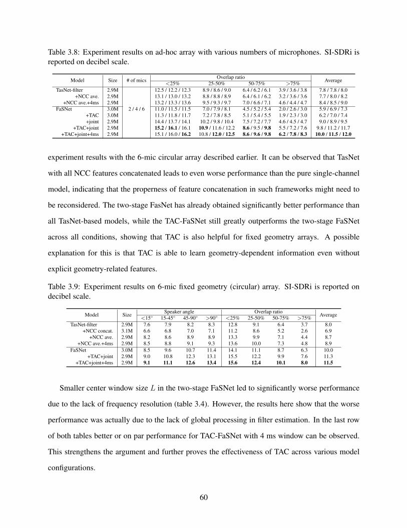
Table 3.8: Experiment results on ad-hoc array with various numbers of microphones. SI-SDRi isreported on decibel scale.

Model Size # of mics Overlap ratio Average<25% 25-50% 50-75% >75%

TasNet-filter 2.9M

2 / 4 / 6

12.5 / 12.2 / 12.3 8.9 / 8.6 / 9.0 6.4 / 6.2 / 6.1 3.9 / 3.6 / 3.8 7.8 / 7.8 / 8.0+NCC ave. 2.9M 13.1 / 13.0 / 13.2 8.8 / 8.8 / 8.9 6.4 / 6.1 / 6.2 3.2 / 3.6 / 3.6 7.7 / 8.0 / 8.2

+NCC ave.+4ms 2.9M 13.2 / 13.3 / 13.6 9.5 / 9.3 / 9.7 7.0 / 6.6 / 7.1 4.6 / 4.4 / 4.7 8.4 / 8.5 / 9.0FaSNet 3.0M 11.0 / 11.5 / 11.5 7.0 / 7.9 / 8.1 4.5 / 5.2 / 5.4 2.0 / 2.6 / 3.0 5.9 / 6.9 / 7.3

+TAC 3.0M 11.3 / 11.8 / 11.7 7.2 / 7.8 / 8.5 5.1 / 5.4 / 5.5 1.9 / 2.3 / 3.0 6.2 / 7.0 / 7.4+joint 2.9M 14.4 / 13.7 / 14.1 10.2 / 9.8 / 10.4 7.5 / 7.2 / 7.7 4.6 / 4.5 / 4.7 9.0 / 8.9 / 9.5

+TAC+joint 2.9M 15.2 / 16.1 / 16.1 10.9 / 11.6 / 12.2 8.6 / 9.5 / 9.8 5.5 / 7.2 / 7.6 9.8 / 11.2 / 11.7+TAC+joint+4ms 2.9M 15.1 / 16.0 / 16.2 10.8 / 12.0 / 12.5 8.6 / 9.6 / 9.8 6.2 / 7.8 / 8.3 10.0 / 11.5 / 12.0

experiment results with the 6-mic circular array described earlier. It can be observed that TasNet

with all NCC features concatenated leads to even worse performance than the pure single-channel

model, indicating that the properness of feature concatenation in such frameworks might need to

be reconsidered. The two-stage FasNet has already obtained significantly better performance than

all TasNet-based models, while the TAC-FaSNet still greatly outperforms the two-stage FaSNet

across all conditions, showing that TAC is also helpful for fixed geometry arrays. A possible

explanation for this is that TAC is able to learn geometry-dependent information even without

explicit geometry-related features.

Table 3.9: Experiment results on 6-mic fixed geometry (circular) array. SI-SDRi is reported ondecibel scale.

Model Size Speaker angle Overlap ratio Average<15° 15-45° 45-90° >90° <25% 25-50% 50-75% >75%

TasNet-filter 2.9M 7.6 7.9 8.2 8.3 12.8 9.1 6.4 3.7 8.0+NCC concat. 3.1M 6.6 6.8 7.0 7.1 11.2 8.6 5.2 2.6 6.9

+NCC ave. 2.9M 8.2 8.6 8.9 8.9 13.3 9.9 7.1 4.4 8.7+NCC ave.+4ms 2.9M 8.5 8.8 9.1 9.3 13.6 10.0 7.3 4.8 8.9

FaSNet 3.0M 8.5 9.6 10.7 11.4 14.1 11.1 8.7 6.3 10.0+TAC+joint 2.9M 9.0 10.8 12.3 13.1 15.5 12.2 9.9 7.6 11.3

+TAC+joint+4ms 2.9M 9.1 11.1 12.6 13.4 15.6 12.4 10.1 8.0 11.5

Smaller center window size L in the two-stage FaSNet led to significantly worse performance

due to the lack of frequency resolution (table 3.4). However, the results here show that the worse

performance was actually due to the lack of global processing in filter estimation. In the last row

of both tables better or on par performance for TAC-FaSNet with 4 ms window can be observed.

This strengthens the argument and further proves the effectiveness of TAC across various model

configurations.

60

3.3 iFaSNet: Implicit Filter-and-sum with Improved Feature Extraction

Both two-stage FaSNet and TAC-FaSNet are based on the problem formulation of an ex-

plicit filter-and-sum operation on the mixture waveforms. However, conventional time-domain

filter-and-sum beamformers have shown to be less effective than frequency-domain filter-and-sum

beamformers. Motivated by the TasNet framework where the masking in the frequency domain is

replaced by the masking in a learnable hidden representation, it is thus natural to consider the filter-

and-sum operation in a learnable representation rather than the waveform domain. Implicit FaSNet

(iFaSNet) marks an attempt to perform implicit filter-and-sum with improved cross-channel feature

extraction.

3.3.1 Modifications upon the TAC-FaSNet

iFaSNet contains four main modifications compared with the TAC-TasNet. First, the origi-

nal multi-input-multi-output (MIMO) formulation is compared with the multi-input-single-output

(MISO) formulation, where the filter is only estimated for the reference channel instead of all the

channels. Second, the filter estimation in a learnable latent space is investigated upon the original

waveform-domain. Third, better cross-channel features that are more suitable for the MISO and

latent-space filtering design are explored. Fourth, a context-aware processing is proposed to further

improve the model performance.

The training target for the standard FaSNet is typically the reverberant clean signals. In the

problem configuration where the time-domain filter-and-sum operation is applied, it implies that

the beamforming filters should not only enhance the signal coming from a certain direction, but

also reconstruct all the reverberation components. However, as reverberation may come from

all possible directions, the ideal beampattern of such beamforming filters might be hard or even

impossible to define. Although FaSNet applies frame-level beamforming where infinite optimal

frame-level filters may exist since the linear equation in equation (3.2) is underdetermined (L equa-

tions and M × (1 + 2W ) unknowns), finding such reverberation-preserving filters for all channels

61

C

Context encoding

D

··· Encoder ···

Feature-level NCC

···

DPRNN+TAC Context decoding

A

···

DecoderMultiply-

and-average

DB

Figure 3.5: Flowchart for the iFaSNet architecture. The modifications to the TAC-FaSNet arehighlighted, which include (A) the use of MISO design instead of the original MIMO design,(B) the use of implicit filtering in the latent space instead of the original explicit filtering on thewaveforms, (C) the use of feature-level NCC feature for cross-channel information instead of theoriginal sample-level NCC feature, and (D) the use of context-aware filtering instead of the originalcontext-independent filtering.

may still be unnecessary. It is natural to consider an alternative problem formulation rather than the

standard filter-and-sum formulation. Since the standard FaSNet estimates a set of filters for each

of the channels and can be viewed as a multi-input-multi-output (MIMO) system, a simple way

to bypass the issue of bad beampatterns is to change it into a multi-input-single-output (MISO)

system where only the filter for the reference channel is estimated. The features from all the

other channels are thus viewed as additional information to assist the separation on a (randomly)

selected reference channel. This reformulates the multi-channel separation problem back to the

single-channel separation problem, while the input to the model still contains the mixtures from

all channels. Figure 3.5 (A) shows the MISO module.

Most existing neural beamformers are mainly designed in the frequency domain due to the fact

that oracle frequency-domain beamformers typically have better performance than those in time

domain. As frequency-domain beamformers are typically formulated as a multiplication operation

on the spectrums, a similar operation can be defined in time-domain systems as a multiplication

operation on learnable features. Note that recent single-channel speech separation systems have

widely applied a set of learnable encoder and decoder to replace the short-time Fourier transform

62

(STFT) and estimated a multiplicative mask on the encoder outputs to match the formulation in

time-frequency masking systems. The formulation of implicit filtering can thus be connected to

the masking operation in such systems.

The extraction of the channel-wise features in the standard FaSNet is calculated on the context

of input mixture frame xi with a corresponding hop size (which is empirically set to L/2), which

results in a sequence of encoder outputs [f it−C , . . . , fit, . . . , f

it+C ] ∈ R(1+2C)×N where t denotes the

frame index and C denotes the context size. The estimated filter with shape R1×N is only applied

to f it, while all encoder outputs of the context are used as the input the filter estimation modules. A

decoder with its weight P ∈ RN×L is applied to transform the filtered feature back to waveforms.

Figure 3.5 (B) shows the newly-added decoder module.

The cross-channel feature in standard FaSNet is calculated by time-domain normalized cross

correlation (tNCC) defined in equation (3.8). The rationale behind tNCC is to capture both the de-

lay information across channels and the source-dependent information for different targets. How-

ever, whether tNCC is still a good feature in the implicit filtering formulation is unknown. Since

implicit filtering operates in the feature space and does not explicitly requires the information of

sample-level delay, it is necessary to modify tNCC such that it better explores the cross-channel

information in the feature level. Here the tNCC is modified to a feature-level NCC (fNCC) feature.

Denote the context feature [f it−C , . . . , fit, . . . , f

it+C ] as Fi

t, fNCC calculates the cosine similarity be-

tween the contextual feature in the reference channel F1t and the contextual feature in all channels

{Fit}Mi=1:

qit = F1t F

iTt (3.18)

where Fit denotes the column-normalized feature of Fi

t where each column has a unit length, and

qit ∈ R(1+2C)×(1+2C) denotes the fNCC feature at time t for channel i. qit is then flatten to a vector

of shape 1× (1 + 2C)2. For the default setting in FaSNet where W = L = 16 ms = 256 samples

with a 50% hop size, C = 2 and (1 + 2C)2 = 25 � 1 + 2W = 513. Figure 3.5 (C) shows the

63

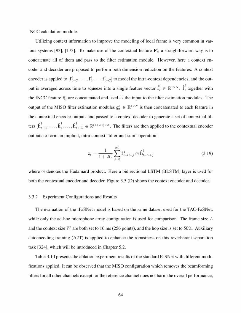
fNCC calculation module.

Utilizing context information to improve the modeling of local frame is very common in var-

ious systems [93], [173]. To make use of the contextual feature Fit, a straightforward way is to

concatenate all of them and pass to the filter estimation module. However, here a context en-

coder and decoder are proposed to perform both dimension reduction on the features. A context

encoder is applied to [f it−C , . . . , fit, . . . , f

it+C ] to model the intra-context dependencies, and the out-

put is averaged across time to squeeze into a single feature vector fi

t ∈ R1×N . fi

t together with

the fNCC feature qit are concatenated and used as the input to the filter estimation modules. The

output of the MISO filter estimation modules g1t ∈ R1×N is then concatenated to each feature in

the contextual encoder outputs and passed to a context decoder to generate a set of contextual fil-

ters [h1

t−C , . . . , h1

t , . . . , h1

t+C ] ∈ R(1+2C)×N . The filters are then applied to the contextual encoder

outputs to form an implicit, intra-context “filter-and-sum” operation:

z1t =

1

1 + 2C

2C∑j=0

f1t−C+j � h

1

t−C+j (3.19)

where � denotes the Hadamard product. Here a bidirectional LSTM (BLSTM) layer is used for

both the contextual encoder and decoder. Figure 3.5 (D) shows the context encoder and decoder.


The evaluation of the iFaSNet model is based on the same dataset used for the TAC-FaSNet,

while only the ad-hoc microphone array configuration is used for comparison. The frame size L

and the context size W are both set to 16 ms (256 points), and the hop size is set to 50%. Auxiliary

autoencoding training (A2T) is applied to enhance the robustness on this reverberant separation

task [324], which will be introduced in Chapter 5.2.

Table 3.10 presents the ablation experiment results of the standard FaSNet with different modi-

fications applied. It can be observed that the MISO configuration which removes the beamforming

filters for all other channels except for the reference channel does not harm the overall performance,

64

Table 3.10: Experiment results with various model configurations. SI-SDRi is reported on decibelscale.

Model Size # of mics Overlap ratio Average<25% 25-50% 50-75% >75%

FaSNet 2.9M

2 / 4 / 6

15.0 / 15.3 / 14.8 10.7 / 11.1 / 11.6 8.6 / 9.2 / 9.3 5.4 / 7.0 / 7.0 9.7 / 10.8 / 10.9+MISO 2.9M 14.8 / 15.5 / 15.7 10.4 / 11.3 / 11.9 8.5 / 9.0 / 9.4 5.0 / 6.8 / 7.1 9.5 / 10.8 / 11.2+fNCC 3.0M 14.5 / 14.8 / 14.4 10.1 / 11.0 / 11.3 8.3 / 8.9 / 9.0 4.9 / 6.7 / 6.9 9.3 / 10.4 / 10.6

+MISO+fNCC 2.9M 15.0 / 15.7 / 15.7 10.6 / 11.4 / 12.2 8.4 / 9.4 / 9.6 5.3 / 7.4 / 8.0 9.7 / 11.1 / 11.6+MISO+implicit 2.9M 14.2 / 14.9 / 15.2 9.8 / 10.9 / 11.3 7.7 / 8.1 / 8.7 4.6 / 5.7 / 6.1 8.9 / 10.0 / 10.6

+MISO+implicit+fNCC 3.0M 15.3 / 16.0 / 16.1 10.9 / 11.8 / 12.5 8.5 / 9.6 / 10.1 5.7 / 7.6 / 8.3 9.9 / 11.4 / 12.0+MISO+implicit+fNCC+context 3.0M 15.6 / 16.4 / 16.5 11.2 / 12.4 / 12.9 9.0 / 10.1 / 10.3 5.8 / 7.9 / 8.8 10.2 / 11.8 / 12.3

and the performance in the 6 microphone setting is even improved. This results supports the previ-

ous discussion that jointly using explicit filter-and-sum formulation and setting reverberant clean

signals as training targets might not be a proper configuration. For the role of the cross-channel

features in different model settings, the results show that using fNCC together with the original

MIMO configuration leads to worse performance than using the original tNCC feature, while us-

ing fNCC together with the MISO configuration can improve the separation performance in high

overlapped utterances. This shows that proper cross-channel features should be selected to keep

inline with the system’s problem formulation in order to achieve a good performance. Applying

MISO configuration together with tNCC feature and implicit filtering achieves even worse perfor-

mance than the baseline FaSNet, while changing the tNCC feature to fNCC feature results in a

performance boost. Since fNCC is calculated on the contextual encoder outputs and the implicit

filtering configuration estimates multiplicative filters on the center frame of the contextual encoder

outputs, this further verifies that matching the problem formulation with a proper cross-channel

feature is crucial for a good overall performance. The last ablation experiment verifies the effec-

tiveness of the context encoder and decoder modules. With a slightly increased model size, the

intra-context filter-and-sum formulation can further improve the performance upon the implicit

filtering formulation, which shows that exploring contextual information is beneficial. This can

also be related to recent literature in multi-tap beamformers where the beamforming filters are

estimated for a context of frames [311].

Table 3.11 compares the training and inference speed for different model configurations. When

the MISO, implicit filtering, and fNCC feature are applied, the training and inference speeds are 2

times and 2.2 times faster, respectively. Adding the context encoder and decoder modules makes

65

Table 3.11: Training and inference speeds of different model configurations. The speeds are mea-sured on a single NVIDIA TITAN Pascal graphic card with a batch size of 4.

Model Training speed Inference speedFaSNet 268.0 ms 98.1 ms

+MISO 222.6 ms 93.2 ms+fNCC 331.7 ms 105.7 ms

+MISO+fNCC 333.0 ms 105.8 ms+MISO+implicit 187.9 ms 96.6 ms

+MISO+implicit+fNCC 132.2 ms 44.2 ms+MISO+implicit+fNCC+context 156.7 ms 52.5 ms

the network slightly slower, but the training and inference speeds are still 1.7 times and 1.9 times

faster than the standard FaSNet, respectively. The results show that iFaSNet does not sacrifice

complexity for performance.

3.4 Discussions

The FaSNet series of work are mainly designed for the ad-hoc microphone array configura-

tion where the microphone number and geometry information are assumed unknown. As FaSNet

applies end-to-end training with a time-domain objective, the comparison between FaSNet and

conventional beamformers as well as frequency-domain neural beamformers needs to consider

either the signal quality or the effect on ASR performance.

In practical applications, the TAC module requires cross-channel feature synchronization in the

average stage. While in ad-hoc microphone array this does not contain the cost of synchronization,

in ad-hoc device configurations where multiple devices with varying numbers of microphones in

each device, how such synchronization across devices should be performed needs further investi-

gation.

66

Chapter 4: Lightweight Model Design for Speech Separation

Model size and complexity remain the biggest challenges in the deployment of speech en-

hancement and separation systems on low-resource devices such as earphones and hearing aids.

Although methods such as compression, distillation and quantization can be applied to large mod-

els, they often come with a cost on the model performance. In this chapter I will introduce two

simple yet effective methods to design ultra-lightweight low-complexity speech separation mod-

els, namely the group communication (GroupComm) method [288] and the context codec method

[289], [326]. GroupComm splits a high-dimensional feature into groups of low-dimensional fea-

tures and applies a module to capture the inter-group dependency. A model can then be applied to

the groups in parallel with a significantly smaller width. A context codec is applied to decrease the

length of a sequential feature, where a context encoder compresses the temporal context of local

features into a single feature representing the global characteristics of the context, and a context

decoder decompresses the transformed global features back to the context features. Combining the

two methods gives the GC3 design for general lightweight sequence modeling module design.

4.1 Related Works

Tremendous efforts have been made to propose novel model architectures and model compres-

sion techniques. Early deep neural networks used for source separation contained stacked recurrent

layers such as LSTM layers with a relatively large number of hidden units [80], [123], [148], [173],

[198], and the corresponding model sizes were typically over tens of millions of parameters with

high model complexity. Convolutional neural networks (CNNs) have also been explored in both

time-frequency domain [137], [146], [165], [204], [302], [312] and time domain [211], [214],

[240], [243], [248], [305], [316], and researchers have begun to focus on decreasing the model size

67

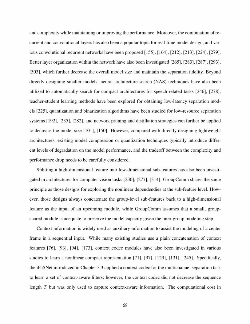
and complexity while maintaining or improving the performance. Moreover, the combination of re-

current and convolutional layers has also been a popular topic for real-time model design, and var-

ious convolutional recurrent networks have been proposed [155], [164], [212], [213], [224], [279].

Better layer organization within the network have also been investigated [265], [283], [287], [293],

[303], which further decrease the overall model size and maintain the separation fidelity. Beyond

directly designing smaller models, neural architecture search (NAS) techniques have also been

utilized to automatically search for compact architectures for speech-related tasks [246], [278],

teacher-student learning methods have been explored for obtaining low-latency separation mod-

els [225], quantization and binarization algorithms have been studied for low-resource separation

systems [192], [235], [282], and network pruning and distillation strategies can further be applied

to decrease the model size [101], [150]. However, compared with directly designing lightweight

architectures, existing model compression or quantization techniques typically introduce differ-

ent levels of degradation on the model performance, and the tradeoff between the complexity and

performance drop needs to be carefully considered.

Splitting a high-dimensional feature into low-dimensional sub-features has also been investi-

gated in architectures for computer vision tasks [230], [277], [314]. GroupComm shares the same

principle as those designs for exploring the nonlinear dependendies at the sub-feature level. How-

ever, those designs always concatenate the group-level sub-features back to a high-dimensional

feature as the input of an upcoming module, while GroupComm assumes that a small, group-

shared module is adequate to preserve the model capacity given the inter-group modeling step.

Context information is widely used as auxiliary information to assist the modeling of a center

frame in a sequential input. While many existing studies use a plain concatenation of context

features [76], [93], [94], [173], context codec modules have also been investigated in various

studies to learn a nonlinear compact representation [71], [97], [129], [131], [245]. Specifically,

the iFaSNet introduced in Chapter 3.3 applied a context codec for the multichannel separation task

to learn a set of context-aware filters; however, the context codec did not decrease the sequence

length T but was only used to capture context-aware information. The computational cost in

68

iFaSNet is thus even higher than that without context codec. The main role of the context codec in

the GC3 framework is to decrease the computational cost in the actual sequence modeling module

by decreasing the sequence length.

4.2 GC3: Group Communication with Context Codec for Ultra-lightweight Long Sequence

Modeling

Group communication (GroupComm) [288] is a module motivated by subband and multiband

processing models such as frequency-LSTM (F-LSTM) [107], [168], [175], [238], which can eas-

ily change a model into an ultra-lightweight counterpart. GroupComm splits a high-dimensional

feature, such as a spectrum, into groups of low-dimensional features, such as subband spectra,

and uses the same model across all the groups for weight sharing. Another inter-group module

is applied to capture the dependencies within the groups, so that the processing of each group al-

ways depends on the global information available. Compared with conventional F-LSTM or other

similar architectures that explicitly model time and frequency dependencies where the subband

features are concatenated back to the fullband feature [127], [132], [222], GroupComm does not

perform such concatenation but simply applies a small module to communicate across the groups.

Moreover, the low-dimensional features enable the use of a smaller module, e.g., CNN or RNN

layer, than the original high-dimensional feature, and together with weight sharing the total model

size can be significantly reduced. A context codec module is applied together with GroupComm

to maintain the performance while further decrease the number of MAC operations, accelerate the

training speed and alleviate the memory consumption in both training and inference time. A con-

text codec module contains a context encoder and a context decoder, where the context encoder

summarizes the temporal context of local features into a single feature representing the global char-

acteristics of the context, and a context decoding module transforms the compressed feature back

to the context features. Squeezing the input contexts into higher-level representations corresponds

to a nonlinear downsampling step that can significantly decrease the length of a feature sequence.

Note that compared with other architectures that perform iterative downsampling and upsampling

69

steps [211], [305], the context codec is only applied once and all remaining modeling steps are ap-

plied on the downsampled features, which enables a smaller memory footprint and faster training

speed. The combination of GroupComm and Context Codec is called the GC3 design.

SeparationModuleSeparation

ModuleN

TSeparation

Module N

T N

T

K=N/M

T

T

N

(A) (B)

(C)

GroupComm Module

SeparationModule

N

T

N

T

···

N

C

N

C

DPRNN/TCN/ Transformer/···

GroupComm Module

SeparationModuleR N

1

N

···

R

N

1

N

···

R

···

N

C

N

C

R

BLSTM GroupComm Module

ContextEncoder

BLSTM GroupComm Module

ContextDecoder

DPRNN/TCN/ Transformer/···

Figure 4.1: Flowcharts for (A) standard sequence processing pipeline with a large sequence mod-eling module; (B) GroupComm-based pipeline, where the features are split into groups with aGroupComm module for inter-group communication. A smaller module for sequence modeling isthen shared by all groups; (C) GC3-based pipeline, where the sequence is first segmented into localcontext frames, and each context is encoded into a single feature. The sequence of summarizedfeatures is passed to a GroupComm-based module in (B). The transformed summarized featuresand the original local context frames are passed to a context decoding module and an overlap-addoperation to generate the output with the same size as the input sequence.

4.2.1 Design of GC3 Module

Given a high-dimensional feature vector h ∈ RN , h can be decomposed into K groups of low-

dimensional feature vectors {gi}Ki=1 with gi ∈ RM . N = KM when there is no overlap between

the groups. A group communication (GroupComm) module is applied across the group of vectors

to capture the inter-group dependencies:

{gi}Ki=1 = F({gi}Ki=1) (4.1)

70

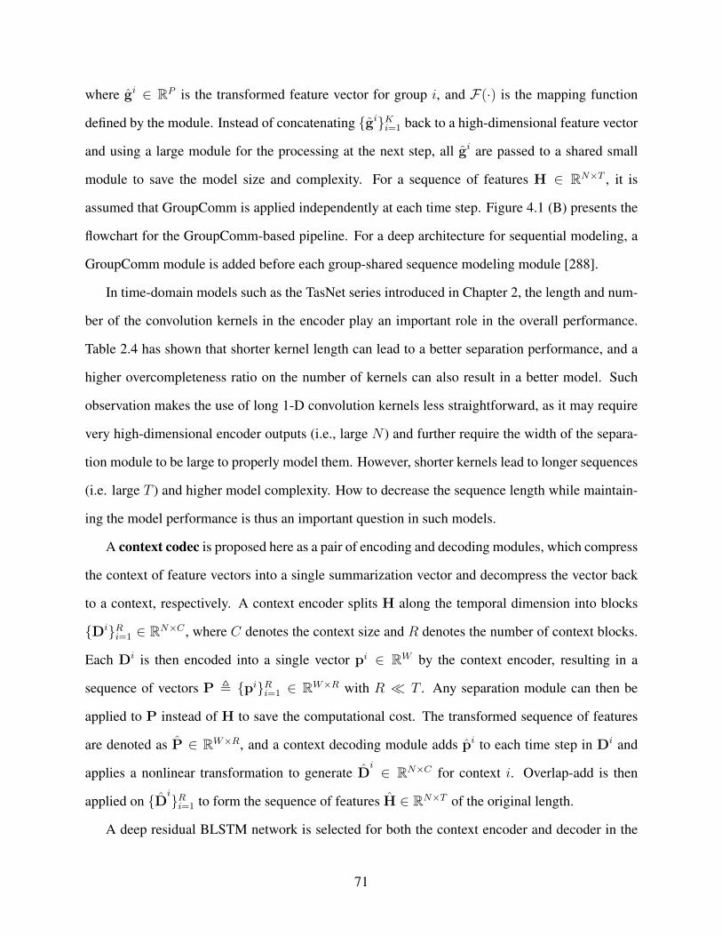
where gi ∈ RP is the transformed feature vector for group i, and F(·) is the mapping function

defined by the module. Instead of concatenating {gi}Ki=1 back to a high-dimensional feature vector

and using a large module for the processing at the next step, all gi are passed to a shared small

module to save the model size and complexity. For a sequence of features H ∈ RN×T , it is

assumed that GroupComm is applied independently at each time step. Figure 4.1 (B) presents the

flowchart for the GroupComm-based pipeline. For a deep architecture for sequential modeling, a

GroupComm module is added before each group-shared sequence modeling module [288].

In time-domain models such as the TasNet series introduced in Chapter 2, the length and num-

ber of the convolution kernels in the encoder play an important role in the overall performance.

Table 2.4 has shown that shorter kernel length can lead to a better separation performance, and a

higher overcompleteness ratio on the number of kernels can also result in a better model. Such

observation makes the use of long 1-D convolution kernels less straightforward, as it may require

very high-dimensional encoder outputs (i.e., large N ) and further require the width of the separa-

tion module to be large to properly model them. However, shorter kernels lead to longer sequences

(i.e. large T ) and higher model complexity. How to decrease the sequence length while maintain-

ing the model performance is thus an important question in such models.

A context codec is proposed here as a pair of encoding and decoding modules, which compress

the context of feature vectors into a single summarization vector and decompress the vector back

to a context, respectively. A context encoder splits H along the temporal dimension into blocks

{Di}Ri=1 ∈ RN×C , where C denotes the context size and R denotes the number of context blocks.

Each Di is then encoded into a single vector pi ∈ RW by the context encoder, resulting in a

sequence of vectors P , {pi}Ri=1 ∈ RW×R with R � T . Any separation module can then be

applied to P instead of H to save the computational cost. The transformed sequence of features

are denoted as P ∈ RW×R, and a context decoding module adds pi to each time step in Di and

applies a nonlinear transformation to generate Di ∈ RN×C for context i. Overlap-add is then

applied on {Di}Ri=1 to form the sequence of features H ∈ RN×T of the original length.

A deep residual BLSTM network is selected for both the context encoder and decoder in the

71

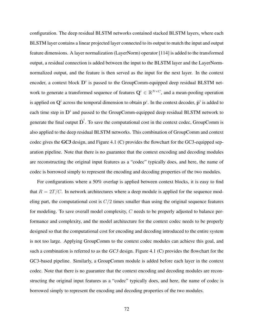
configuration. The deep residual BLSTM networks contained stacked BLSTM layers, where each

BLSTM layer contains a linear projected layer connected to its output to match the input and output

feature dimensions. A layer normalization (LayerNorm) operator [114] is added to the transformed

output, a residual connection is added between the input to the BLSTM layer and the LayerNorm-

normalized output, and the feature is then served as the input for the next layer. In the context

encoder, a context block Di is passed to the GroupComm-equipped deep residual BLSTM net-

work to generate a transformed sequence of features Qi ∈ RN×C , and a mean-pooling operation

is applied on Qi across the temporal dimension to obtain pi. In the context decoder, pi is added to

each time step in Di and passed to the GroupComm-equipped deep residual BLSTM network to

generate the final output Di. To save the computational cost in the context codec, GroupComm is

also applied to the deep residual BLSTM networks. This combination of GroupComm and context

codec gives the GC3 design, and Figure 4.1 (C) provides the flowchart for the GC3-equipped sep-

aration pipeline. Note that there is no guarantee that the context encoding and decoding modules

are reconstructing the original input features as a “codec” typically does, and here, the name of

codec is borrowed simply to represent the encoding and decoding properties of the two modules.

For configurations where a 50% overlap is applied between context blocks, it is easy to find

that R = 2T/C. In network architectures where a deep module is applied for the sequence mod-

eling part, the computational cost is C/2 times smaller than using the original sequence features

for modeling. To save overall model complexity, C needs to be properly adjusted to balance per-

formance and complexity, and the model architecture for the context codec needs to be properly

designed so that the computational cost for encoding and decoding introduced to the entire system

is not too large. Applying GroupComm to the context codec modules can achieve this goal, and

such a combination is referred to as the GC3 design. Figure 4.1 (C) provides the flowchart for the

GC3-based pipeline. Similarly, a GroupComm module is added before each layer in the context

codec. Note that there is no guarantee that the context encoding and decoding modules are recon-

structing the original input features as a “codec” typically does, and here, the name of codec is

borrowed simply to represent the encoding and decoding properties of the two modules.

72


GC3 is evaluated on the same single-channel separation task with the identical dataset de-

scribed in Chapter 3.2.2. The TasNet framework is used as the backbone network design for all

experiments. All models use 2 ms window size in the waveform encoder and decoder and ReLU

nonlinearity as the activation function for the mask estimation layer. For GroupComm-based and

GC3-based models, a GroupComm module is added before each layer in the separator, and the

width of the layers is modified according to the number of groups K. The mask estimation layer

in GroupComm-based and GC3-based models is shared by all the groups. The number of groups

in the context codec is also set to be the same as that in the separator blocks. The notations for the

hyperparameters can be found in table 4.1. The implementation of all models is available online1.

Three model architectures are compared for the GroupComm module:

1. BLSTM: A standard residual BLSTM layer is applied to all the groups to model the intra-

group dependencies.

2. Transform-average-concatenate (TAC) [286]: TAC was proposed for the multichannel speech

separation task with ad-hoc microphone arrays where no microphone indexing or geometry

information is known in advance. The design particularly matches the need in the Group-

Comm module where “group indices”, i.e., the sequential order of the features in different

groups, does not exist. For the group of features {gi}Ki=1, a fully-connected (FC) layer with

parametric rectified linear unit (PReLU) activation [99] is applied for the transformation

step:

f i = P (gi) (4.2)

where P (·) is the mapping function defined by the first FC layer and f i ∈ RD denotes the

output for group i. All f i are then averaged and passed to the second FC layer with PReLU

1https://github.com/yluo42/GC3

73

https://github.com/yluo42/GC3

activation for the averaging step:

f = R(1

K

K∑i=1

f i) (4.3)

where R(·) is the mapping function defined by the second FC layer and f ∈ RD is the output

for this step. f is finally concatenated with the output of the transformation step, f i, and

passed to a third FC layer with PReLU activation to generate the final output gi:

gi = S([f i; f ]) (4.4)

where S(·) is the mapping function defined by the third FC layer and [x;y] denotes the

concatenation operation of vectors x and y. A residual connection is finally added between

the module input gi and output gi.

3. Multi-head Self Attention (MHSA) [166]: MHSA is widely used in various sequence model-

ing tasks and has already proven its effectiveness in multiple speech-related problems [166],

[184], [233], [237], [252]. MHSA explicitly models the relationship between each pair of

group features and thus can capture sequence-level dependencies. Following the standard

definition of MHSA, the concatenation of group features {gi}Ki=1 is rewritten into a matrix

G ∈ RK×M and apply a MHSA layer:

Hn = Softmax(QnK

Tn√

dk)Vn (4.5)

G′n = [H1; · · · ; Hn]Wo (4.6)

where n is the number of attention heads, Wqn,W

kn,W

vn ∈ RM×dk are the linear transfor-

mation matrices for head n, Qn = GWqn, Kn = GWk

n, and Vn = GWvn are the linear

transformations for query, key and value, respectively, Hn ∈ RK×dk is the output at head n,

and Wo is the linear transformation matrix for the output. Both the concatenation operation

74

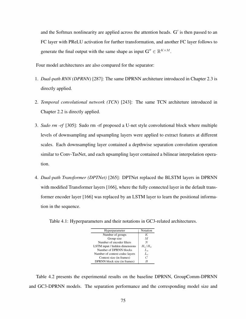
and the Softmax nonlinearity are applied across the attention heads. G′ is then passed to an

FC layer with PReLU activation for further transformation, and another FC layer follows to

generate the final output with the same shape as input G′′ ∈ RK×M .

Four model architectures are also compared for the separator:

1. Dual-path RNN (DPRNN) [287]: The same DPRNN architeture introduced in Chapter 2.3 is

directly applied.

2. Temporal convolutional network (TCN) [243]: The same TCN architeture introduced in

Chapter 2.2 is directly applied.

3. Sudo rm -rf [305]: Sudo rm -rf proposed a U-net style convolutional block where multiple

levels of downsampling and upsampling layers were applied to extract features at different

scales. Each downsampling layer contained a depthwise separation convolution operation

similar to Conv-TasNet, and each upsampling layer contained a bilinear interpolation opera-

tion.

4. Dual-path Transformer (DPTNet) [265]: DPTNet replaced the BLSTM layers in DPRNN

with modified Transformer layers [166], where the fully connected layer in the default trans-

former encoder layer [166] was replaced by an LSTM layer to learn the positional informa-

tion in the sequence.

Table 4.1: Hyperparameters and their notations in GC3-related architectures.

Hyperparameter NotationNumber of groups K

Group size MNumber of encoder filters N

LSTM input / hidden dimensions Hi/Ho

Number of DPRNN blocks Ls

Number of context codec layers Lc

Context size (in frames) CDPRNN block size (in frames) B

Table 4.2 presents the experimental results on the baseline DPRNN, GroupComm-DPRNN

and GC3-DPRNN models. The separation performance and the corresponding model size and

75

Table 4.2: Comparison of DPRNN, GroupComm-DPRNN and GC3-DPRNN TasNet models withdifferent hyperparameter configurations. MACs are calculated on 4-second mixtures.

Model K M N Hi / Ho Ls Lc C B SI-SDR (dB) Model size MACsDPRNN 1 128 128 64 / 128 6 – – 100 9.0 2.6M 22.1G

GroupComm-DPRNN

2 64 128 64 / 128 4

– – 100

9.5 2.6M (99.4%) 43.4G (196.4%)4 32 128 32 / 64 4 9.4 663.0K (25.3%) 22.4G (101.4%)8 16 128 16 / 32 4 8.9 175.5K (6.7%) 11.9G (53.8%)

168 128 8 / 16 4 8.1 51.9K (2.0%) 6.6G (29.9%)

6 8.9 73.5K (2.8%) 9.6G (43.4%)

16 256 16 / 32 2 8.1 100.7K (3.8%) 12.4G (56.1%)4 9.7 183.9K (7.0%) 23.7G (107.2%)

324 128 4 / 8 6 7.6 26.0K (1.0%) 5.7G (25.8%)

10 8.5 37.6K (1.4%) 9.1G (41.2%)

8 256 8 / 16 2 7.9 38.7K (1.5%) 7.2G (32.6%)4 8.6 60.3K (2.3%) 13.2G (59.7%)

GC3-DPRNN

4 32 128 32 / 64 4 1

32 24 8.9

881.5K (33.7%)

9.2G (41.6%)16 32 8.8 10.6G (48.0%)8 50 8.8 13.3G (60.2%)4 64 9.3 18.6G (84.2%)

8 16 128 16 / 32 6 1

32 24

8.7 314.4K (12.0%) 5.4G (24.4%)2 9.3 369.9K (14.1%) 8.1G (36.7%)

16 8 128 8 / 16 8 2 8.9 124.1K (4.7%) 5.4G (24.4%)16 256 16 / 32 6 1 9.0 322.9K (12.3%) 10.9G (49.3%)

32 4 128 4 / 8 14 2 8.3 57.1K (2.2%) 3.6G (16.3%)8 256 8 / 16 8 9.2 132.6K (5.1%) 10.7G (48.4%)

complexity for the three types of models are reported. Model complexity is measured by the

number of MAC operations (MACs), and the MACs for all models are calculated by an open-

source toolbox2. First notice that when K is small (e.g. K ≤ 4), the GroupComm-DPRNN

models can achieve higher performance than plain DPRNN with smaller model size at the cost of

an on par or higher model complexity. This is due to the extra MAC operations introduced by the

GroupComm module. A largerK leads to fewer MAC operations; however, the depth of the model

has to be modified accordingly to maintain the performance. Different hyperparameter settings are

explored such that for each K a model with less than 5% relative performance degradation can

be obtained. Among all the GroupComm-DPRNN models, the model with K = 16, N = 128

and Ls = 6 achieves on par performance as the standard DPRNN model with 2.8% model size

and 43.4% MAC operations, and the model with K = 32, N = 128 and Ls = 10 only has 5%

performance degradation with 1.4% model size and 41.2% MAC operations. These models show

that GroupComm is effective in decreasing both the model size and complexity without sacrificing

the performance. Moreover, experiments on the effect of model width in terms of N and Hi/Ho

2https://github.com/Lyken17/pytorch-OpCounter

76

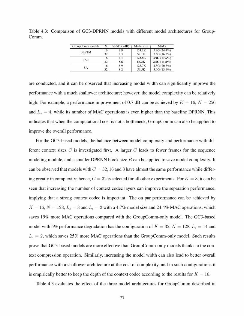
https://github.com/Lyken17/pytorch-OpCounter

Table 4.3: Comparison of GC3-DPRNN models with different model architectures for Group-Comm.

GroupComm module K SI-SDR (dB) Model size MACs

BLSTM 16 8.9 124.1K 5.4G (24.4%)32 8.3 57.1K 3.6G (16.3%)

TAC 16 9.1 123.8K 3.9G (17.6%)32 8.6 56.3K 2.6G (11.8%)

SA 16 8.9 123.7K 4.5G (20.3%)32 8.2 56.5K 3.0G (13.4%)

are conducted, and it can be observed that increasing model width can significantly improve the

performance with a much shallower architecture; however, the model complexity can be relatively

high. For example, a performance improvement of 0.7 dB can be achieved by K = 16, N = 256

and Ls = 4, while its number of MAC operations is even higher than the baseline DPRNN. This

indicates that when the computational cost is not a bottleneck, GroupComm can also be applied to

improve the overall performance.

For the GC3-based models, the balance between model complexity and performance with dif-

ferent context sizes C is investigated first. A larger C leads to fewer frames for the sequence

modeling module, and a smaller DPRNN block size B can be applied to save model complexity. It

can be observed that models withC = 32, 16 and 8 have almost the same performance while differ-

ing greatly in complexity; hence, C = 32 is selected for all other experiments. ForK = 8, it can be

seen that increasing the number of context codec layers can improve the separation performance,

implying that a strong context codec is important. The on par performance can be achieved by

K = 16, N = 128, Ls = 8 and Lc = 2 with a 4.7% model size and 24.4% MAC operations, which

saves 19% more MAC operations compared with the GroupComm-only model. The GC3-based

model with 5% performance degradation has the configuration of K = 32, N = 128, Ls = 14 and

Lc = 2, which saves 25% more MAC operations than the GroupComm-only model. Such results

prove that GC3-based models are more effective than GroupComm-only models thanks to the con-

text compression operation. Similarly, increasing the model width can also lead to better overall

performance with a shallower architecture at the cost of complexity, and in such configurations it

is empirically better to keep the depth of the context codec according to the results for K = 16.

Table 4.3 evaluates the effect of the three model architectures for GroupComm described in

77

Table 4.4: Effect of group overlap ratio on model complexity and separation performance in GC3-DPRNN models.

Group overlap SI-SDR (dB) Model size MACs0% 9.1

123.8K3.9G (17.6%)

25% 9.0 4.9G (22.0%)50% 9.4 6.9G (31.3%)

Chapter 4.2.1. For the TAC architecture, the hidden dimension for transform and average layers is

set to 3Ho. For the MHSA architecture, four attention heads with the hidden dimension dk set toM

are applied. Such configurations are applied to match the overall model sizes with a BLSTM layer.

The hyperparameter configurations of the two GC3-based models marked in bold in table 4.2 with

K = 16 and 32 are selected. The results show that although MHSA achieves on par performance

as BLSTM in both configurations, TAC obtains even better performance with the fewest MAC

operations. Since the number of MAC operations in TAC is fewer than those in both BLSTM and

MHSA and the transformation and concatenation steps in TAC can be run in parallel across groups,

TAC is used as the default module for GroupComm in all remaining experiments.

The default group segmentation configuration in all experiments above assumes no overlap

between groups. However, a 50% overlap is always applied in sequence segmentation operations

such as context segmentation in the context codec and block segmentation in DPRNN modules.

It is thus interesting to see whether adding overlap between groups can improve the performance.

Table 4.4 provides the separation performance as well as the model size and complexity for differ-

ent overlap ratios between groups. It can be observed that adding a 25% percent overlap between

groups increases the number of MAC operations while not leading to an better performance, but

a 50% overlap between groups can improve the overall performance. Compared with the model

in table 4.2 with a similar performance (K = 8, N = 128, Lc = 2), such a model has a smaller

model size and fewer MAC operations. This shows that compared with using a smaller number

of groups K, adding proper overlap between groups is a more effective method for improving the

performance.

To evaluate GC3 on the four model architectures for the separator, the hyperparameters are

selected so that all four models have on-par model size when no GroupComm or context codec are

78

Table 4.5: Comparison of DPRNN, TCN, Sudo rm -rf, and DPTNet architectures with and withoutGC3. The training and inference phase statistics are evaluated with a batch size of 4.

Model SI-SDR (dB) PESQ STOI Model size MACs Training Training Inference Inferencememory (GB) speed (ms) memory (GB) speed (ms)

Mixture -0.4 1.91 0.77 – – – – – –DPRNN [287] 9.0 2.33 0.80 2.6M 22.1G 3.0 193.4 24.9 59.7

+ GC3 9.1 2.36 0.82 123.8K (4.7%) 3.9G (17.6%) 4.2 211.3 6.3 57.2TCN [243] 7.1 2.21 0.80 2.5M 10.3G 3.2 254.6 14.4 53.8

+ GC3 8.9 2.35 0.82 191.2K (7.6%) 3.4G (33.0%) 3.8 194.1 6.6 49.3Sudo rm -rf [305] 6.8 2.15 0.79 2.4M 9.5G 4.6 234.8 14.4 53.5

+ GC3 8.7 2.34 0.81 60.0K (2.5%) 3.2G (33.7%) 3.7 200.3 5.3 47.4DPTNet [265] 8.1 2.20 0.79 2.8M 21.8G 4.8 256.2 21.2 78.6

+ GC3 8.5 2.32 0.81 128.6K (4.6%) 3.9G (17.9%) 4.8 272.5 6.2 76.7

applied:

1. TCN: TCNs with 6 convolutional blocks were selected in each TCN. The same number of

TCN layers and convolutional blocks is applied for the GC3-equipped modification.

2. Sudo rm -rf : The default configuration of the original literature is selected, which contains

5 downsampling and upsampling layers in each U-net block. 8 blocks are used for both

baseline and GC3-equipped modification.

3. DPTNet: The default configuration of the original literature is selected, which contains 6

Transformer layers. 8 Transformer layers is selected for the GC3-equipped DPTNet, which

is similar to the configuration for GC3-DPRNN. The learning rate warm-up configuration is

also set the same as the recommended configuration, where the first 4000 iterations are used

for the warm-up stage.

The other hyperparameters are kept the same as the selected best GC3-DPRNN model in Ta-

ble 4.3. Table 4.5 presents the separation performance as well as the model size and complexity

of the four architectures with their GC3-equipped modifications. First, the plain DPRNN archi-

tecture achieves the best performance among the four architectures and is even better than the

plain DPTNet, which indicates that transformer-based architectures might not be always superior

than recurrent neural networks. TCN does not have satisfying performance because of the limited

receptive field in the configuration (253 frames or 0.253s), as it has been shown that large recep-

tive fields for TCN lead to better separation performance [243]. Although the selected Sudo rm

79

-rf configuration has a large enough receptive field to cover the entire sequential feature, it ob-

tains an even worse separation performance with on-par model size and complexity as the TCN

architecture. Although [305] reported that the Sudo rm -rf architecture achieved constantly better

performance than DPRNN and TCN architectures, the results here indicates that its performance

on the more challenging noisy reverberant environments needs to be revised. Moreover, although

all four architectures achieve significant SI-SDR improvement with respect to the unprocessed

mixture, the improvement on wideband PESQ and STOI scores are moderate. One possible reason

for this phenomenon is the inconsistency between the time-domain and frequency-domain evalu-

ation metrics [243], as all the models are trained with the time-domain objective (negative SNR)

while the calculation of PESQ and STOI are both in frequency domain.

For DPRNN and DPTNet, GC3-equipped modifications can achieve a same level of separation

performance with significantly smaller model sizes and number of MAC operations. For CNN-

based architectures (TCN and Sudo rm -rf), GC3-equipped modifications can further achieve sig-

nificantly higher SI-SDR scores. Since the context codec squeezes the long sequence by a factor

of C/2 (16 for C = 32), the effective temporal receptive field of the TCN separator is significantly

larger (0.253 × 16 = 4.05s) and thus can better capture the temporal dependencies. Since it has

also been reported in [305] that a deeper Sudo rm -rf architecture can lead to better overall sep-

aration performance, introducing GC3 to Sudo rm -rf might also be equivalent to increasing the

model depth and improves the performance. More in-depth analysis on the reason behind the per-

formance improvements in different architectures is left for future work. Nevertheless, the results

prove that GC3 can be easily deployed in to various architectures and maintain its effectiveness.

Beyond the model size and number of MAC operations, the memory footprint and the training

and inference speed are also important indicators for model complexity, as small models can also

be slow and require enormous memory. To compare such training and inference phase statistics

of different models, the batch-level training and inference phase memory footprints and running

speeds are evaluated on a single NVIDIA TITAN X Pascal graphic card with a batch size of 4.

80

The memory footprint is calculated via an opensource toolbox 3. It can be observed that the GC3-

equipped models, e.g. DPRNN and TCN, increase the training phase memory footprint but do

not affect the training speed, and an acceleration can even be observed in the GC3-equipped TCN

model. The inference phase memory footprint for all four architectures with GC3 applied are sig-

nificantly lower than the ones without GC3, however the inference speed are all on-par or only

slightly faster than the baselines. The reason for this might be because the effective model depth

for a GC3-equipped model is larger than the baseline which prevents the model from easy paral-

lelization. The results show that although the number of intermediate outputs introduced by the

deeper separation module and the GroupComm modules may increase the training phase memory

footprint, GC3 can always decrease the inference phase memory footprint without sacrificing the

inference speed.

4.3 Discussions

Note that the application of model binarization or quantization techniques are not jointly con-

sidered with GC3. Such techniques can significantly decrease the model storage size and MAC

operations without changing the model architecture, although they typically lead to certain levels

of performance degradation [250]. Applying GC3 together with such techniques may require an in-

crease in the overall model size to achieve on par performance, and the actual model configuration

may be directly related to the target platform to which the model will be deployed. Moreover, the

GroupComm module can be used as a prototype module in any neural architecture search (NAS)

algorithm [197] to search for better both model architecture and layer organization, balancing the

model size, complexity and performance.

3https://github.com/Stonesjtu/pytorch_memlab

81

Chapter 5: Training Objectives for Speech Separation

In this chapter I will introduce two training objectives for speech separation in different con-

ditions. Both objectives rely on auxiliary autoencoding, which adds an autoencoding loss to the

standard training objectives, e.g., SNR and SI-SDR, to tackle certain problems in speech separa-

tion. The auxiliary autoencoding permutation invariant training (A2PIT) [290] was proposed for

separating varying numbers of sources in the mixtures with a single network, which was based on

a design principle called do nothing is better than do wrong things. The auxiliary autoencoding

training (A2T) [324] was designed for improving the system robustness in reverberant environ-

ments, which put constraints on the search space of the network during optimization to find better

separation results.

5.1 Related works

5.1.1 Training Methods for Separating Varying Numbers of Sources

Various methods have been proposed to tackle the problem of separating varying numbers of

sources in an end-to-end model. A most simple way is to assume a maximum number of sources

in a mixture, which is denoted by N , and let the model to always generate N outputs [148],

[239]. For mixtures having M sources where M < N , N −M outputs are invalid and need to

be properly designed and effectively detected. The invalid outputs are typically forced to have a

significantly smaller energy than the valid outputs, and a energy threshold can then be applied to

filter out those outputs. Another approach first estimates the speaker embedding for each active

source with an output-length-free model, e.g. a sequence-to-sequence generative model, and then

performs speaker extraction based on the embeddings [249]. A third category of methods perform

separation in an iterative way, where in each iteration only one target source is separated from the

82

residual mixture [193], [210], [247], [251]. The iteration stops when there is no source left, and

the stop time can be determined by either an energy threshold or another trained discriminator. It

has been shown that under various circumstances, the number of sources in the mixture can be

effectively estimated and the separation performance can be guaranteed. Moreover, clustering-

based approaches have been extensively applied in frequency-domain separation systems, where

the T-F masks are treated as the cluster assignment matrices and the number of clusters can be

dynamically decided for different mixtures [121], [123], [140], [151], [218], [242].

5.1.2 Training Methods for Separation in Reverberant Environments

Both end-to-end systems and T-F domain systems for anechoic speech enhancement and sepa-

ration can be directly applied in the reverberant scenarios [268]. For systems that do not attempt to

perform joint enhancement/separation and dereverberation, a mapping function is typically learned

between the reverberant mixture and the reverberant clean signals with either single-channel or

multi-channel input [231], [241], [273], [286]. The evaluation of such systems is also done by

comparing the system outputs with the reverberant clean signals. One exception is the convolu-

tive transfer function invariant signal-to-distortion ratio (CI-SDR) [263], which is essentially the

standard SDR metric, where the adaptive FIR filter is applied to the separation outputs before

the calculation of the SI-SDR metric. Experiment results in a multi-channel separation task with

MVDR beamforming showed that CI-SDR is beneficial for both signal quality measured in SDR

and speech recognition measured in WER.

5.2 A2PIT: Separating Varying Numbers of Sources

There are various drawbacks in each category of the existing methods. For the fixed-output-

number method, the training targets for the invalid outputs are typically low- or zero-energy sig-

nals. However, such targets cannot be jointly used with energy-invariant training objectives, such

as scale-invariant signal-to-distortion ratio (SI-SDR) [236], which has proven to be a better training

objective in many scenarios [284]. Moreover, the detection of invalid outputs typically relies on a

83

pre-defined energy threshold, which may cause trouble when the mixture also has very low energy.

For the speaker extraction method, the speaker embeddings are typically estimated at utterance

level and require a long enough context, which makes the method hard to apply to online or causal

systems. For methods that utilize additional target speaker enrollments for speaker embedding

extraction, the generalization ability on unseen speakers is also limited. For the iterative method,

the run-time complexity linearly increases as the number of sources increases, and stop time de-

tection is typically performed at utterance level as well. When there is noise in the mixture, it is

also unclear in which iteration should the noise be cancelled. Moreover, none of the methods has

a “fault tolerance” mechanism when the estimated number of sources is different than the actual

number. What should the model append to the output if it estimates fewer sources than the actual

case? How should the model remove invalid outputs if it generates more? How can such decision

process or control flow be effectively incorporated into the training of the model? These questions

are important for a practical and robust system.

A simple training method based on the fixed-output assumption is proposed here by designing

proper training targets for the invalid outputs. The fixed-output-number assumption is adopted as

in real-world conversations such as meeting scenarios, the maximum number of simultaneously

active speakers is almost always fewer than three [30], [259], thus a maximum number of speakers

can typically be pre-assumed. Instead of using low-energy auxiliary targets for invalid outputs,

the mixture itself is used as auxiliary targets to force the invalid outputs to perform autoencoding.

With the permutation invariant training (PIT) framework [173] for speech separation, the training

objective is referred to it as the auxiliary autoencoding permutation invariant training (A2PIT).

A2PIT not only allows the model to perform valid output detection in a self-supervised way without

additional modules, but also achieves “fault tolerance” by the “do nothing is better than do wrong

things” principle. As the mixture itself can be treated as the output of a null separation model, i.e.

perform no separation at all, the auxiliary targets force the model to generate outputs not worse

than doing nothing. Moreover, the detection of invalid outputs in A2PIT can be done at frame-level

based on the similarity between the outputs and the mixture, which makes it possible to perform

84

single-pass separation and valid source detection in real-time.

5.2.1 Motivation and Design

There are two main issues in the energy-based method for invalid output detection. First, it

cannot be jointly used with energy-invariant objective functions like SI-SDR. Second, once the

detection of invalid speakers fails and the noise signals are selected as the targets, the outputs

can be completely uncorrelated with any of the targets, which is unpreferred for applications that

require high perceptual quality or low distortion. It is defined as the problem of lacking “fault

tolerance” mechanism for unsuccessful separation.

To allow the models to use any objective functions and to have such “fault tolerance” ability,

the mixture signal itself is selected as the auxiliary targets instead of random noise signals. For

mixtures with N outputs and M < N targets, N −M mixture signals are appended to the targets

and PIT is applied to find the best output permutation with respect to the targets. The A2PIT loss

with the best permutation then becomes:

Lobj = Lsep + LAE (5.1)

where Lsep ∈ R is the loss for the valid outputs and LAE ∈ R is the auxiliary autoencoding loss for

the invalid outputs with the input mixture as targets. As autoencoding is in general a much simpler

task than separation, proper gradient balancing method should be applied on the two loss terms for

successful training. Recall that SI-SDR is defined as:

SI-SDR(x, x) = 10 log10

||αx||22||x− αx||22

(5.2)

where α = xx>/xx> corresponds to the optimal rescaling factor towards the estimated signal. Let

85

a , xx>, b , xx> and c , xx>, the definition can be rewritten as:

SI-SDR(x, x) = 10 log10

(b2/a

c− 2b2/a+ b2/a

)= 10 log10

(1

ac/b2 − 1

), 10 log10

(c(x, x)2

1− c(x, x)2

) (5.3)

where c(x, x) , b/√ac = xx>/

√(xx>)(xx>) is the cosine similarity between x and x. The

scale-invariance behavior of SI-SDR can be easily observed by the nature of cosine similarity, and

SI-SDR(x, x) → +∞ as |c(x, x)| → 1. It’s easy to see that the second term in the derivative of

SI-SDR with respect to the cosine similarity, |∂ SI-SDR(x, x)/∂ c(x, x)|, approaches infinity as

|c(x, x)| approaches 1. Using it for LAE may let the system to easily collapse to a local minimum

which have very high performance on the auxiliary autoencoding term while fail to separate the

sources. Based on this concern, an α-skewed SI-SDR (α-SI-SDR) is proposed here:

α-SI-SDR(x, x) , 10 log10

(c(x, x)2

1 + α− c(x, x)2

)(5.4)

where the scale of the gradient with respect to the cosine similarity term is controlled by α ≥ 0,

and α = 0 corresponds to the standard SI-SDR. For multiple-speaker utterances, α = 0.3 is

empirically set for LAE and α = 0 is set for Lsep. For single-speaker utterances, the training target

for separation is equivalent (when there is no noise) or very close (when there is noise) to the input

mixture. In this case, α = 0.3 is also set for Lsep.

5.2.2 Detection of Invalid Outputs

During inference phase, the detection of invalid outputs can be performed by calculating the

similarity, e.g. SI-SDR score, between all outputs and the input mixture, and a threshold calcu-

lated from the training set can be used for the decision. For the “fault tolerance” mechanism, the

following method is applied for selecting the valid outputs:

86

1. If the estimated number of outputsK is smaller than the actual numberM ,M−K additional

outputs are randomly selected from the N −K remaining outputs.

2. If the estimated number of outputs K is larger than the actual number M , M outputs are

randomly selected from the K outputs.

Another benefit for A2PIT is that it also allows frame-level detection of the invalid outputs for

causal applications. Frame-level detection calculates accumulated similarity starting from the first

frame of the outputs, and is able to dynamically change the selected valid outputs as the similarity

scores become more reliable. For streaming-based applications that require a real-time playback

of the separation outputs, e.g. hearable devices, the change of the output tracks can also be easily

done by switching the outputs at frame-level.


A simulated single-channel noisy speech separation dataset with the Librispeech dataset [109]

is used for the experiments. 40 hours of training data, 20 hours of validation data, and 12 hours of

test data are generated from the 100-hour training set, development set, and test set, respectively.

The number of speakers are evenly sampled between 1 and 4 to make sure the dataset is balanced

to the varying numbers of speakers. All utterances are 6-second long with a sample rate of 16k Hz.

For utterances with more than one speaker, an overlap ratio between all the speakers is uniformly

sampled between 0% and 100% and the speech signals are shifted accordingly. The speech signals

are then rescaled to a random absolute energy between -2.5 and 2.5 dB. A noise signal is randomly

selected from the 100 Nonspeech Corpus [334], and is repeated if its length is less than 6 seconds.

The noise signal is then rescaled to a random absolute energy between -20 and -10 dB. Both the

clean and noisy mixtures are used to report the performance of A2PIT in the two scenarios.

The DPRNN-TasNet introduced in Chapter 2.3 is used for all experiments. The same hyper-

parameter settings of 2 ms window configuration is applied with the only difference that 3 instead

of 6 DPRNN blocks is applied. The total number of parameters is thus 1.3M. The baseline model

uses the standard SI-SDR as the training objective, and all other models use the proposed A2PIT

87

together with α-SI-SDR. All models are trained for a maximum of 100 epochs with the Adam

optimizer [83]. The initial learning rate is 1e− 3 and is decayed by a factor of 0.98 for every two

epochs. No other regularizers or training tricks are applied. The DPRNN-TasNet models trained

for each of the speaker count configurations are used as the baseline models, and these results

represents how well the models can achieve when the number of speakers is known and a specific

model is trained on such mixtures. For separating varying numbers of sources, the DPRNN-TasNet

models are trained on three configurations:

1. 2+3 speakers: the 2 and 3 speaker mixtures are used for both training and evaluation, and the

number of outputs N is set to 3. This is to mimic the behavior under certain cases when the

maximum number of active sources is bounded by 3 (e.g. meeting scenarios). It is denoted

as the 2+3 model.

2. 2+3+4 speakers: the 2, 3 and 4 speaker mixtures are used for both training and evaluation,

and the number of outputs N is set to 4. This is to increase the difficulty of both the separa-

tion and speaker count. It is denoted as the 2+3+4 model.

3. 1+2+3+4 speakers: all training and evaluation datasets are used. It is denoted as the 1+2+3+4

model.

Each configuration contains both the clean and noisy scenarios, which results in a total of 6

different configurations.

Table 5.1 and 5.2 show the confusion matrices for all 6 configurations. Note that each of the

speaker number has a test set of 1800 utterances. First notice that for the 2+3 model, the prediction

of speaker count can be done with a very high accuracy in both clean and noisy separation tasks.

For the 2+3+4 model, the detection of 3 speaker mixtures is worse than that of both 2 and 4

speaker mixtures, and the error mostly comes from the misclassification into 4 speaker mixtures.

For the 1+2+3+4 model, the detection of the 1 speaker mixtures almost always fail (detects no

speakers in the mixture). With the autoencoding threshold, the model predicts no valid outputs for

most of the times. This is somehow expected as in the clean separation task, the mixture itself is

88

Table 5.1: Confusion matrix for speaker counting for models trained for clean separation task.

Model PredictionOracle

1 spk 2 spk 3 spk 4 spk2+3

model2 spk – 1712 5 –3 spk – 88 1795 –

2+3+4model

2 spk – 1718 10 03 spk – 82 1435 264 spk – 0 355 1774

1+2+3+4model

1 spk 2 0 0 02 spk 5 1746 13 23 spk 0 62 1454 444 spk 0 0 333 1756

Table 5.2: Confusion matrix for speaker counting for models trained for noisy separation task.

Model PredictionOracle

1 spk 2 spk 3 spk 4 spk2+3

model2 spk – 1716 26 –3 spk – 83 1774 –

2+3+4model

2 spk – 1711 16 03 spk – 87 1530 874 spk – 1 254 1713

1+2+3+4model

1 spk 31 4 0 02 spk 5 1670 8 03 spk 0 125 1485 274 spk 0 0 307 1773

89

equivalent to the separated output, and in the noisy separation task, the separated output may still

have very high similarity score with respect to the mixture because of the high SNR configuration.

For tasks such as automatic speech recognition, this will not be an issue as the acoustic models

are typically noise robust, while for tasks that require perceptual quality, the outputs need to be

further evaluated. Beyond the 1 speaker mixtures, the accuracy for speaker counting for other

cases remains high. Another interesting observation is that the models occasionally predict zero

speakers (e.g. 2-speaker utterances in all models for noisy separation). This can only happen when

the autoencoding SI-SDR of all outputs are larger than the pre-defined threshold. It indicates that

in certain utterances the separation may completely fail and the model converges to always perform

autoencoding. A better solution to this issue is left for future works.

Figure 5.1: Histograms of autoencoding SI-SDR (decibel scale) in different experiment configura-tions.

Table 5.3: Separation performance of various configurations on the clean separation task. SI-SDRis reported for one speaker utterances on decibel scale, and SI-SDRi is reported for the rest ondecibel scale.

ModelOutput

selectionSI-SDR SI-SDRi

1 spk 2 spk 3 spk 4 spkBaseline Oracle 64.8 11.5 8.0 5.7

2+3model

Oracle – 12.0 8.8 –Predicted – 11.6 8.7 –

2+3+4model

Oracle – 11.8 9.1 7.1Predicted – 11.7 8.1 7.1

1+2+3+4model

Oracle 39.8 11.9 9.1 7.2Predicted 44.2 11.8 8.5 7.2

90

Table 5.4: Separation performance of various configurations on the noisy separation task. SI-SDRiis reported in decibel scale.

ModelOutput

selectionSI-SDRi

1 spk 2 spk 3 spk 4 spkBaseline Oracle 6.9 10.8 7.5 5.4

2+3model

Oracle – 11.2 8.7 –Predicted – 11.2 8.7 –

2+3+4model

Oracle – 11.1 8.8 7.0Predicted – 10.8 8.2 6.9

1+2+3+4model

Oracle 4.8 11.1 8.8 6.9Predicted 4.2 11.0 8.4 6.9

Table 5.3 and 5.4 provide the separation performance on the clean and noisy separation tasks,

respectively. For the one speaker utterances in the clean separation task, SI-SDR instead of SI-

SDRi is reported as the input is already the clean target itself. It can be observed that A2PIT can

almost always improve the separation performance on all configurations with both clean and noisy

data, and the gains for 3 and 4 speaker cases are significant. It can be concluded from the results

that A2PIT is able to achieve on par or better overall separation performance on both clean and

noisy separation tasks. Even with predicted output selection, the fault tolerance ability introduced

by A2PIT allows the model to control the performance degradation. These results confirms the

effectiveness of A2PIT.

5.3 A2T: Distortion-controlled Separation in Noisy Reverberant Environments

Using the reverberant clean signal as both the training and evaluation targets introduces new

challenges to the current training and evaluation configurations. One core problem, which is re-

ferred to as the equal-valued contour problem, occurs in many widely-used metrics such as signal-

to-noise ratio (SNR) and scale-invariant signal-to-distortion ratio (SI-SDR). Equal-valued contour

problem denotes the issue that given a reference signal and a metric, there are infinite numbers of

estimated signals that can achieve the same performance. Certain estimations among this “contour”

might be more preferred than the others, however an end-to-end model may lack the ability to dis-

tinguish the “good” estimations from the “bad” ones. As an example of the equal-valued contour

91

problem in reverberant separation, consider an ideal model that always separates the direct-path

targets from the reverberant mixture. When evaluated by the signal-level metric between the sepa-

ration outputs and the reverberant targets, the model will not obtain a high performance especially

when the energy of the late reverberation component is large (e.g. with a large reverberation time).

However, such an ideal model can achieve very good performance on both word-error-rate (WER)

and subjective perceptual quality measures. Suppose there is another model that achieves similar

performance as this ideal model when evaluated by the signal-level metric while performs noisy,

distorted separation, it is easy to imagine that this model will achieve a much worse performance.

The equal-valued contour problem mainly comes from the training configurations where a sin-

gle end-to-end training objective is used without further regularizations on the distortion introduced

to components such as the direct-path signals. It is natural to investigate how such regularizations

can be incorporated into the training procedure in a simple way. The focus here is on the end-

to-end systems where the separation is done by applying a linear mapping, e.g. a multiplicative

mask, on the input mixture. This framework includes many recently proposed systems, including

the TasNet-series of works in Chapter 2 and any linear neural beamformers in Chapter 3. With the

linearity between the input and output, an additional auxiliary autoencoding loss is added, which

forces the linear mapping to also perform autoencoding on the direct-path target signal. For exam-

ple, given a mixture signal which contains one target signal x and K ≥ 1 additional interference

signals {ni}Ki=1, standard training configuration attempts to optimize the model to learn a linear

mappingM(·) such thatM(x +∑K

i=1 ni) ≈ x. The auxiliary autoencoding term corresponds to

the reconstruction of the direct-path signal of x, denoted by xd, i.e. M(xd) ≈ xd. This training

configuration is referred to as the auxiliary autoencoding training (A2T).

5.3.1 Motivation and Design

The problem formulation of end-to-end reverberant speech enhancement and separation is

briefly reviewed first. Given M channels of inputs and C signal-of-interests (SOIs), the mixture

92

signal at channel i is represented as:

yi =C∑j=1

x(j)i + ni, i ∈ 1, . . . ,M (5.5)

where x(j)i ∈ R1×T is the j-th SOI at channel i and ni ∈ R1×T is the interference at channel i.

In reverberant environment, each SOI is obtained by convolving a clean signal c(j)i ∈ R1×(T−K+1)

with a room impulse response (RIR) filter h(j)i ∈ R1×K :

x(j)i = c

(j)i ∗ h(j)

i (5.6)

By decomposing the RIR filter h(j)i into a direct path RIR hd

(j)i and a late reverberation RIR hr

(j)i ,

the SOI x(j)i can be decomposed into a direct path signal x(j)

d,i and a late reverberation signal x(j)r,i :

x(j)i = c

(j)i ∗ h(j)

i

= c(j)i ∗ (hd

(j)i + hr

(j)i )

, x(j)d,i + x

(j)r,i

(5.7)

The task of speech enhancement or separation is to extract the SOIs given the mixtures. Here

the end-to-end systems that generate a linear mapping T (·) between the mixture and each estimated

SOI is considered:

{x(j)}Cj=1

= T({yi}Mi=1

)(5.8)

In typical configurations, the training objective is to minimize the discrepancy between the

estimated and the target SOIs at a specific reference microphone:

Lobj =C∑j=1

D(x(j),x

(j)1

)(5.9)

93

where D(·) is a metric on the two signals, and it is assumed that the first channel is selected as the

reference channel without loss of generality.

(A) SNR

(B) SI-SDR

Figure 5.2: Simplified illustrations for equal-valued contours in (A) SNR metric, and (B) SI-SDRmetric.

The equal-valued contour problem can then be demonstrated in two widely-used metrics,

94

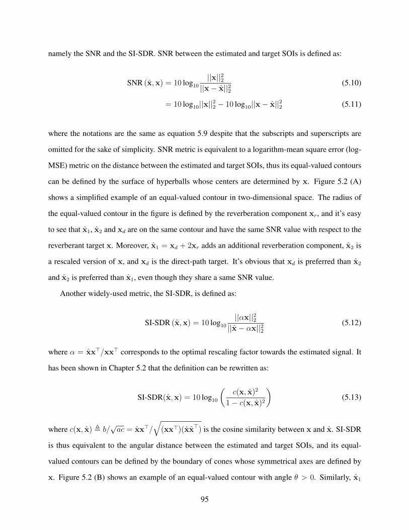
namely the SNR and the SI-SDR. SNR between the estimated and target SOIs is defined as:

SNR (x,x) = 10 log10

||x||22||x− x||22

(5.10)

= 10 log10||x||22 − 10 log10||x− x||22 (5.11)

where the notations are the same as equation 5.9 despite that the subscripts and superscripts are

omitted for the sake of simplicity. SNR metric is equivalent to a logarithm-mean square error (log-

MSE) metric on the distance between the estimated and target SOIs, thus its equal-valued contours

can be defined by the surface of hyperballs whose centers are determined by x. Figure 5.2 (A)

shows a simplified example of an equal-valued contour in two-dimensional space. The radius of

the equal-valued contour in the figure is defined by the reverberation component xr, and it’s easy

to see that x1, x2 and xd are on the same contour and have the same SNR value with respect to the

reverberant target x. Moreover, x1 = xd + 2xr adds an additional reverberation component, x2 is

a rescaled version of x, and xd is the direct-path target. It’s obvious that xd is preferred than x2

and x2 is preferred than x1, even though they share a same SNR value.

Another widely-used metric, the SI-SDR, is defined as:

SI-SDR (x,x) = 10 log10

||αx||22||x− αx||22

(5.12)

where α = xx>/xx> corresponds to the optimal rescaling factor towards the estimated signal. It

has been shown in Chapter 5.2 that the definition can be rewritten as:

SI-SDR(x,x) = 10 log10

(c(x, x)2

1− c(x, x)2

)(5.13)

where c(x, x) , b/√ac = xx>/

√(xx>)(xx>) is the cosine similarity between x and x. SI-SDR

is thus equivalent to the angular distance between the estimated and target SOIs, and its equal-

valued contours can be defined by the boundary of cones whose symmetrical axes are defined by

x. Figure 5.2 (B) shows an example of an equal-valued contour with angle θ > 0. Similarly, x1

95

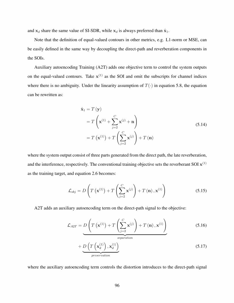
and xd share the same value of SI-SDR, while xd is always preferred than x1.

Note that the definition of equal-valued contours in other metrics, e.g. L1-norm or MSE, can

be easily defined in the same way by decoupling the direct-path and reverberation components in

the SOIs.

Auxiliary autoencoding Training (A2T) adds one objective term to control the system outputs

on the equal-valued contours. Take x(1) as the SOI and omit the subscripts for channel indices

where there is no ambiguity. Under the linearity assumption of T (·) in equation 5.8, the equation

can be rewritten as:

x1 = T (y)

= T

(x(1) +

C∑j=2

x(j) + n

)

= T(x(1))

+ T

(C∑j=2

x(j)

)+ T (n)

(5.14)

where the system output consist of three parts generated from the direct path, the late reverberation,

and the interference, respectively. The conventional training objective sets the reverberant SOI x(1)

as the training target, and equation 2.6 becomes:

Lobj = D

(T(x(1))

+ T

(C∑j=2

x(j)

)+ T (n) ,x(1)

)(5.15)

A2T adds an auxiliary autoencoding term on the direct-path signal to the objective:

LA2T = D

(T(x(1))

+ T

(C∑j=2

x(j)

)+ T (n) ,x(1)

)︸︷︷︸

separation

(5.16)

+D(T(x

(1)d

),x

(1)d

)︸︷︷︸

preservation

(5.17)

where the auxiliary autoencoding term controls the distortion introduces to the direct-path signal

96

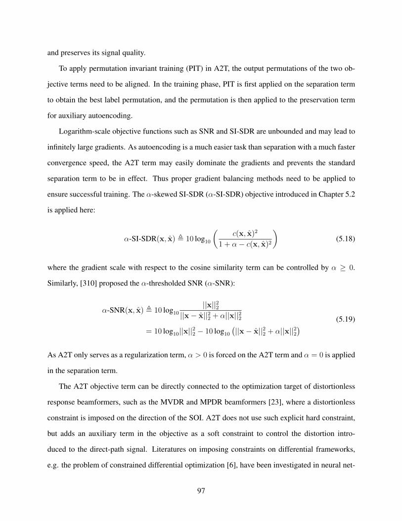
and preserves its signal quality.

To apply permutation invariant training (PIT) in A2T, the output permutations of the two ob-

jective terms need to be aligned. In the training phase, PIT is first applied on the separation term

to obtain the best label permutation, and the permutation is then applied to the preservation term

for auxiliary autoencoding.

Logarithm-scale objective functions such as SNR and SI-SDR are unbounded and may lead to

infinitely large gradients. As autoencoding is a much easier task than separation with a much faster

convergence speed, the A2T term may easily dominate the gradients and prevents the standard

separation term to be in effect. Thus proper gradient balancing methods need to be applied to

ensure successful training. The α-skewed SI-SDR (α-SI-SDR) objective introduced in Chapter 5.2

is applied here:

α-SI-SDR(x, x) , 10 log10

(c(x, x)2

1 + α− c(x, x)2

)(5.18)

where the gradient scale with respect to the cosine similarity term can be controlled by α ≥ 0.

Similarly, [310] proposed the α-thresholded SNR (α-SNR):

α-SNR(x, x) , 10 log10

||x||22||x− x||22 + α||x||22

= 10 log10||x||22 − 10 log10

(||x− x||22 + α||x||22

) (5.19)

As A2T only serves as a regularization term, α > 0 is forced on the A2T term and α = 0 is applied

in the separation term.

The A2T objective term can be directly connected to the optimization target of distortionless

response beamformers, such as the MVDR and MPDR beamformers [23], where a distortionless

constraint is imposed on the direction of the SOI. A2T does not use such explicit hard constraint,

but adds an auxiliary term in the objective as a soft constraint to control the distortion intro-

duced to the direct-path signal. Literatures on imposing constraints on differential frameworks,

e.g. the problem of constrained differential optimization [6], have been investigated in neural net-

97

Figure 5.3: Illustration of two possible linear mappings T (1)(·) and T (2)(·). T (1)(·) denotes the onelearned with A2T with a controlled distortion on the direct-path signal xd. T (2)(·) corresponds toan unconstrained mapping where the distortion on xd can be significant.

works [110], however soft constraints have shown better performance and easier implementation

than hard constraints [153]. Moreover, unlike MVDR/MPDR which are designed only for multi-

channel systems, A2T can be easily applied to any end-to-end system which satisfies the linearity

assumption of the mapping.

On the other hand, forcing the outputs to meet the A2T constraint may help with the general-

ization of the model. Figure 5.3 shows two example mappings T (1)(·) and T (2)(·) with and without

A2T, respectively. When the distortion introduced to the direct-path xd is significant, the mapping

on the other sources and the noise, i.e. e = y − x, needs to compensate for the distortion in order

to map to the SOI x. As the SOI and the interferences are in general uncorrelated, learning such

a mapping may hurt the performance and the generalization ability of the system. Another point

to clarify is that empirically T (2)(·) might not be the usual case for models without A2T, as the

experiment results will show that standard objectives inherently preserve the direct-path signal to

some extent. Nevertheless, properly adding the A2T term can almost always achieve on par or

better separation performance with a significantly lower distortion on the direct-path signal. This

indicates that A2T is able to find “better” outputs on the equal-valued contours.

98

For the consideration of extra computational costs during training, applying autoencoding on

the direct-path signal only requires the calculation of the linear transform on the direct-path targets.

The complexity for the backward pass is slightly increased as the gradients with respect to the A2T

term also need to be backpropagated, but the overall increase on the computational cost is minor.


The evaluation of the iFaSNet model is based on the same dataset used for the TAC-FaSNet

in Chapter 3.2, while only the ad-hoc microphone array configuration is used for comparison.

As the utterances in the dataset are randomly truncated and not suitable for speech recognition

evaluation, another test set with 500 utterances simulated where the utterances are not truncated.

In order to approximately match the length of the mixtures in the training set, the utterances are

randomly sampled from the test-clean subset whose length is no longer than 4 seconds. All other

configurations are the same as the original dataset.

DPRNN-TasNet is selected for all the models with the identical configuration in Chapter 2.3.

The evaluation of the separation performance is done by both SNR and SI-SDR metrics. To evalu-

ate the distortion introduced to the direct-path signals, the target-SNR (TSDR) and target-SI-SDR

(TSI-SDR) is also applied, which are calculated between the transformed direct-path signal T (xd)

and the direct-path signal xd:

TSNR (x,x) = SNR (T (xd),xd) (5.20)

TSI-SDR (x,x) = SI-SDR (T (xd),xd) (5.21)

The evaluation of the speech recognition performance is done by word error rate (WER). The

recognition engine used is directly taken from the pre-trained transformer model on Librispeech

data from ESPNet [221]1.

Table 5.5 shows the experiment results of models trained with different objective functions,

1https://github.com/espnet/espnet/tree/master/egs/librispeech/asr1

99

Table 5.5: Comparison of DPRNN-TasNet models with objectives with and without A2T on thenoisy reverberant separation task. “OR” stands for the overlap ratio between the two speakers.

Objective αSNR / TSNR / SI-SDR / TSI-SDR (dB)

OR ∈ [0, 25)% OR ∈ [25, 50)% OR ∈ [50, 75)% OR ∈ [75, 100]% OverallSNR – 14.0 / 18.4 / 13.7 / 18.3 10.3 / 12.9 / 9.7 / 12.6 8.0 / 10.3 / 6.9 / 9.7 6.1 / 8.4 / 4.5 / 7.7 9.6 / 12.5 / 8.7 / 12.1

+ A2T

0 -0.4 / 60.6 / -0.4 / 62.1 -0.4 / 60.1 / -0.4 / 61.9 -0.4 / 59.6 / -0.4 / 61.7 -0.5 / 58.8 / -0.5 / 61.3 -0.4 / 59.8 / -0.4 / 61.80.01 12.8 / 26.0 / 12.6 / 26.0 8.3 / 23.3 / 7.9 / 23.4 5.3 / 23.4 / 4.8 / 23.5 2.8 / 24.0 / 2.3 / 24.3 7.3 / 24.2 / 6.9 / 24.30.03 13.8 / 23.0 / 13.5 / 23.2 9.8 / 18.9 / 9.3 / 19.0 7.3 / 16.9 / 6.4 / 16.9 5.2 / 15.6 / 3.9 / 15.7 9.0 / 18.6 / 8.3 / 18.70.1 14.0 / 21.4 / 13.7 / 21.5 10.1 / 16.8 / 9.5 / 16.8 7.8 / 14.6 / 6.9 / 14.5 5.9 / 13.1 / 4.5 / 13.0 9.5 / 16.5 / 8.7 / 16.50.3 14.2 / 20.3 / 13.9 / 20.4 10.5 / 15.7 / 10.0 / 15.6 8.2 / 13.2 / 7.2 / 13.1 6.2 / 11.5 / 4.8 / 11.2 9.8 / 15.2 / 9.0 / 15.11 14.2 / 19.3 / 13.9 / 19.2 10.4 / 14.5 / 9.9 / 14.4 8.1 / 12.0 / 7.1 / 11.8 6.0 / 10.1 / 4.5 / 9.8 9.7 / 14.0 / 8.9 / 13.83 14.3 / 18.9 / 14.0 / 18.9 10.5 / 13.5 / 9.9 / 13.3 8.1 / 10.9 / 7.2 / 10.5 6.1 / 9.0 / 4.5 / 8.5 9.8 / 13.1 / 8.9 / 12.8

10 14.1 / 18.5 / 13.7 / 18.4 10.2 / 13.0 / 9.6 / 12.7 7.8 / 10.3 / 6.7 / 9.7 5.7 / 8.3 / 4.0 / 7.5 9.4 / 12.6 / 8.5 / 12.1SI-SDR – – / – / 13.9 / 16.9 – / – / 9.8 / 10.5 – / – / 6.9 / 7.6 – / – / 4.4 / 5.5 – / – / 8.8 / 10.2

+ A2T

0 – / – / -0.5 / 62.2 – / – / -0.4 / 62.2 – / – / -0.4 / 62.3 – / – / -0.5 / 62.5 – / – / -0.4 / 62.30.01 – / – / 12.4 / 27.0 – / – / 7.6 / 24.9 – / – / 4.3 / 26.3 – / – / 1.8 / 28.3 – / – / 6.6 / 26.60.03 – / – / 13.2 / 23.5 – / – / 8.9 / 19.7 – / – / 5.9 / 19.0 – / – / 3.4 / 19.8 – / – / 7.9 / 20.50.1 – / – / 13.6 / 21.3 – / – / 9.7 / 16.9 – / – / 6.9 / 14.6 – / – / 4.4 / 13.1 – / – / 8.7 / 16.50.3 – / – / 14.0 / 20.8 – / – / 9.8 / 16.0 – / – / 7.0 / 13.6 – / – / 4.5 / 11.9 – / – / 8.8 / 15.61 – / – / 13.9 / 19.8 – / – / 9.9 / 14.9 – / – / 7.2 / 12.3 – / – / 4.7 / 10.5 – / – / 8.9 / 14.43 – / – / 13.9 / 19.5 – / – / 9.9 / 14.4 – / – / 7.3 / 11.9 – / – / 4.8 / 10.0 – / – / 9.0 / 14.0

10 – / – / 14.1 / 19.4 – / – / 9.9 / 14.0 – / – / 7.3 / 11.5 – / – / 4.6 / 9.5 – / – / 9.0 / 13.6

Table 5.6: Comparison of WER from models trained with SNR with and without A2T. “OR” standsfor the overlap ratio between the two speakers.

Objective αWER (%)

OR ∈ [0, 25)% OR ∈ [25, 50)% OR ∈ [50, 75)% OR ∈ [75, 100]% OverallSNR – 15.5 20.8 38.4 60.2 34.2

+ A2T0.3 15.3 17.5 36.4 57.7 32.11 15.2 18.4 36.5 58.8 32.63 14.8 20.5 34.5 59.5 32.8

Noisy reverberant – – – – – 17.7Clean reverberant – – – – – 8.1

with and without A2T, and with different values of α for gradient balancing in the A2T term. For

the models trained with SI-SDR, the SNR and TSNR scores are not reported as SI-SDR does not

preserve the scale of the outputs. First notice that the models trained with original SNR and SI-SDR

objectives are able to inherently control the distortion introduced to the direct-path signals to some

extent, and in low-overlapped utterances the distortion is significantly lower than high-overlapped

utterances. On the one hand, the performance of TSNR and TSI-SDR in low-overlapped utterances

is expected as in the nonoverlapped regions the separation model is equivalent to an autoencoding

model. On the other hand, the worse performance in high-overlapped utterances shows that the

equal-valued contour problem is practical and the separated outputs might not be the preferred

ones. Moreover, SI-SDR objective even leads to a lower TSI-SDR score than the SNR objective

across all overlap ratios. Since the SNR objective is also able to preserve the output scale, the

100

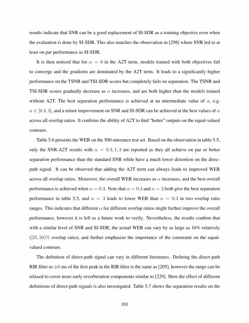
results indicate that SNR can be a good replacement of SI-SDR as a training objective even when

the evaluation is done by SI-SDR. This also matches the observation in [298] where SNR led to at

least on par performance as SI-SDR.

It is then noticed that for α = 0 in the A2T term, models trained with both objectives fail

to converge and the gradients are dominated by the A2T term. It leads to a significantly higher

performance on the TSNR and TSI-SDR scores but completely fails on separation. The TSNR and

TSI-SDR scores gradually decrease as α increases, and are both higher than the models trained

without A2T. The best separation performance is achieved at an intermediate value of α, e.g.

α ∈ [0.3, 3], and a minor improvement on SNR and SI-SDR can be achieved at the best values of α

across all overlap ratios. It confirms the ability of A2T to find “better” outputs on the equal-valued

contours.

Table 5.6 presents the WER on the 500-utterance test set. Based on the observation in table 5.5,

only the SNR-A2T results with α = 0.3, 1, 3 are reported as they all achieve on par or better

separation performance than the standard SNR while have a much lower distortion on the direc-

path signal. It can be observed that adding the A2T term can always leads to improved WER

across all overlap ratios. Moreover, the overall WER increases as α increases, and the best overall

performance is achieved when α = 0.3. Note that α = 0.3 and α = 3 both give the best separation

performance in table 5.5, and α = 3 leads to lower WER than α = 0.3 in two overlap ratio

ranges. This indicates that different α for different overlap ratios might further improve the overall

performance, however it is left as a future work to verify. Nevertheless, the results confirm that

with a similar level of SNR and SI-SDR, the actual WER can vary by as large as 16% relatively

([25, 50)% overlap ratio), and further emphasize the importance of the constraint on the equal-

valued contours.

The definition of direct-path signal can vary in different literatures. Defining the direct-path

RIR filter as±6 ms of the first peak in the RIR filter is the same as [205], however the range can be

relaxed to cover more early reverberation components similar to [229]. Here the effect of different

definitions of direct-path signals is also investigated. Table 5.7 shows the separation results on the

101

Table 5.7: Comparison of DPRNN-TasNet models with direct-path RIR filter defined as the±20 ms of the first peak in the RIR filter.

Objective αSNR / TSNR / SI-SDR / TSI-SDR (dB)

OR ∈ [0, 25)% OR ∈ [25, 50)% OR ∈ [50, 75)% OR ∈ [75, 100]% OverallSNR – 14.0 / 18.7 / 13.7 / 18.6 10.3 / 13.1 / 9.7 / 12.8 8.0 / 10.5 / 6.9 / 10.0 6.1 / 8.6 / 4.5 / 7.8 9.6 / 12.8 / 8.7 / 12.3

+ A2T (±20 ms)0.3 14.1 / 20.3 / 13.8 / 20.3 10.2 / 15.3 / 9.7 / 15.2 7.9 / 12.8 / 6.9 / 12.7 5.9 / 10.9 / 4.3 / 10.7 9.6 / 14.9 / 8.7 / 14.71 14.1 / 19.4 / 13.8 / 19.4 10.4 / 14.2 / 9.8 / 14.0 7.9 / 11.5 / 6.9 / 11.1 5.8 / 9.5 / 4.2 / 9.1 9.6 / 13.7 / 8.7 / 13.43 14.0 / 19.1 / 13.7 / 19.2 10.1 / 13.7 / 9.5 / 13.5 7.8 / 11.0 / 6.7 / 10.7 5.8 / 9.0 / 4.1 / 8.6 9.4 / 13.3 / 8.5 / 13.0

Table 5.8: Comparison of WER from models trained with direct-path RIR filter defined as the±20 ms of the first peak in the RIR filter.

Objective αWER (%)

OR ∈ [0, 25)% OR ∈ [25, 50)% OR ∈ [50, 75)% OR ∈ [75, 100]% OverallSNR – 15.5 20.8 38.4 60.2 34.2

SNR+A2T (±6 ms) 0.3 15.3 17.5 36.4 57.7 32.1

SNR+A2T (±20 ms)0.3 14.8 19.2 38.2 62.1 34.01 15.4 19.2 36.5 61.1 33.43 15.0 19.3 36.8 60.2 33.2

same datasets as above, while the direct-path RIR filter is defined as ±20 ms of the first peak in

the RIR filter. Interestingly, the separation performance measured by SNR and SI-SDR are both

worse than those in table 5.5, and the autoencoding performance measured by TSNR and TSI-

SDR, although on a different definition of direct-path signal, are also worse. The reason might be

that autoencoding on the ±20 ms direct-path signal also suffers the equal-valued contour problem,

as the early reverberations may also cause minor distortions on the overall reconstruction. The

recognition performance presented in table 5.8 also show that the WERs on ±20 ms A2T are

in general worse than those on ±6 ms A2T, while still better than the standard SNR objective.

Moreover, unlike the observation in ±6 ms A2T that a larger α leads to worse WER, a larger α

here leads to better performance. The reason behind this observation is yet to be revealed. To

summarize, A2T prefers a more aggressive definition of direct-path signal.

5.4 Discussions

Both A2PIT and A2T make use of the concept of auxiliary autoencoding. Since the two training

objectives are designed for different purposes, they can be jointly applied in the separation of

varying number of sources in a reverberant environment, which better matches the requirements in

real-world applications.

102

On the other hand, A2T requires the linearity assumption in the separation process, which

might contradict with certain problem definitions which I will introduce in the next chapter. Al-

though A2T is only evaluated on the end-to-end single-channel separation task, its application on

mask-based neural beamformers might also be promising, as the masking operation is a linear

operation and mask-based beamformers have proven effective in tasks such as ASR. Moreover,

although the auxiliary autoencoding loss in A2T is applied on the direct-path signal, it can also

be applied on the interference signal to put constraints on the equal-valued contours on the entire

SOI. The effect of such application is left for future works.

103

Chapter 6: Rethinking the Problem Formulations of End-to-end Speech

Separation

The previous chapters put the focus on new designs for model architectures and training objec-

tives. In this chapter, I take a step back and empirically revisit some of the problem formulations

in the end-to-end separation pipeline. I select three topics in the general end-to-end separation

pipeline: (1) the role and necessity of separation layers [323], where an explicit “separation” op-

eration defined as a single-input-multi-output (SIMO) operation happens at the end of the “separa-

tion” layers; (2) the performance of generalized iterative separation [325], where multiple rounds

of separation is cascaded to form a multi-pass separation procedure; (3) the effect of end-to-end

training, where a time-domain training objective is applied to networks with both time-domain and

frequency-domain encoder and decoder. The dataset used for all the experiments in this chapter is

identical with the one in Chapter 3.2.

6.1 Rethinking the Roles of Separation Layers in Speech Separation Networks

6.1.1 Motivation and Experiment Design

Speech separation models can be broadly categorized into single-input-single-output (SISO)

systems and single-input-multi-output (SIMO) systems. A SISO system usually consists a stack of

one to one mapping layers, extracting one speaker from the mixture at each time. SISO networks

are typically designed for guided source separation (GSS) or speech enhancement tasks [88], [183],

[217], [232], [258], [262], where a bias is often needed to distinguish the target speaker. When

there are more than one source that need to be estimated, the single output separation needs to

be performed multiple times, one for each source. In certain iterative separation methods, a mask

can be estimated from the last layer in the model representing one target source, and a residual

104

signal can be calculated by subtracting the separated output from the mixture [251]. The residual

signal is then used as the input for next iteration. In contrast, the SIMO systems are the standard

design for blind source separation (BSS) [148], [211], [293], [313], which target at separating C

sources simultaneously. To fulfill this task, on top of the one to one mapping layers, there always

exists one or more one-to-many mapping layers that convert the single input signal to multiple

source output, i.e. one to many mapping. For example, in standard masking-based BSS models,

C masks are generally estimated from the last layer in the network. In [227], though named as

“MIMO” network, the system is essentially a SIMO system where the input feature consist of

multi-microphone information.

Researchers have also explored the combination of SIMO and SIMO architecture for further

performance improvement. A commonly applied integration is to use a SISO network for post-

enhancement module on the output of the SIMO separation result [148], [228], [256], [261], while

typically the two modules are not jointly optimized. However, as the combination systems usually

contain a significantly larger parameter size which could also results in potential performance im-

provement for a pure SIMO network, little is known about the roles of SIMO and SISO modules

in a BSS separation system. Why performance improvements can be achieved by incorporating

the SISO modules? For a given model size, how to properly arrange the sizes of SIMO and SISO

modules to achieve a best performance? Are SIMO modules always necessary? Those are the

motivations for an empirical analysis on different model configurations, including the standard

SIMO-only model, the mixed SIMO-SISO models, and the SISO-only models, on their effective-

ness on the separation performance.

The three configurations are compared with a similar model architecture. For model configu-

ration, the same DPRNN-TasNet architecture introduced in Chapter 2.3 is adopted in all formu-

lations. The linear mapping function defined by the waveform encoder in the DPRNN-TasNet is

denoted as E(·), and the waveform encoder and decoder in Figure 6.1 are omitted for the sake of

simplicity.

Figure 6.1 (A) shows the flowchart for the SIMO-only model design, which is the default

105

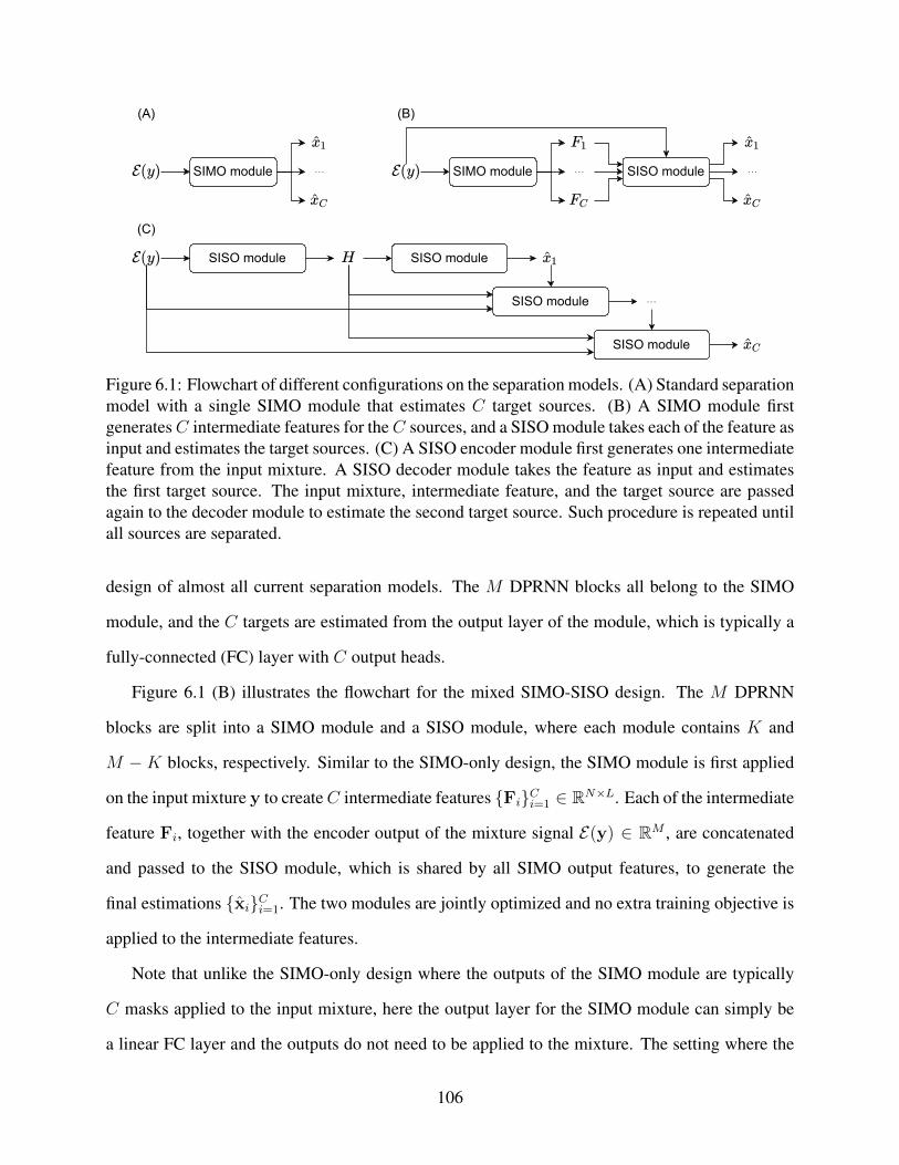
SIMO module SISO module··· ···SIMO module ···

(A) (B)

(C)

SISO module SISO module

SISO module ···

SISO module

Figure 6.1: Flowchart of different configurations on the separation models. (A) Standard separationmodel with a single SIMO module that estimates C target sources. (B) A SIMO module firstgeneratesC intermediate features for theC sources, and a SISO module takes each of the feature asinput and estimates the target sources. (C) A SISO encoder module first generates one intermediatefeature from the input mixture. A SISO decoder module takes the feature as input and estimatesthe first target source. The input mixture, intermediate feature, and the target source are passedagain to the decoder module to estimate the second target source. Such procedure is repeated untilall sources are separated.

design of almost all current separation models. The M DPRNN blocks all belong to the SIMO

module, and the C targets are estimated from the output layer of the module, which is typically a

fully-connected (FC) layer with C output heads.

Figure 6.1 (B) illustrates the flowchart for the mixed SIMO-SISO design. The M DPRNN

blocks are split into a SIMO module and a SISO module, where each module contains K and

M −K blocks, respectively. Similar to the SIMO-only design, the SIMO module is first applied

on the input mixture y to createC intermediate features {Fi}Ci=1 ∈ RN×L. Each of the intermediate

feature Fi, together with the encoder output of the mixture signal E(y) ∈ RM , are concatenated

and passed to the SISO module, which is shared by all SIMO output features, to generate the

final estimations {xi}Ci=1. The two modules are jointly optimized and no extra training objective is

applied to the intermediate features.

Note that unlike the SIMO-only design where the outputs of the SIMO module are typically

C masks applied to the input mixture, here the output layer for the SIMO module can simply be

a linear FC layer and the outputs do not need to be applied to the mixture. The setting where the

106

outputs from the SIMO module are indeed the C masks and the masked mixture encoder output is

directly used as {Fi}Ci=1 is also tested. {Fi}Ci=1 is directly added to the SISO outputs to form the

final separated sources. This matches the standard pipeline in pre-separation and post-enhancement

models, where the SIMO module servers as the pre-separation module and the SISO module is the

post-enhancement module. Empirically such setting leads to identical performance as the simpler

pipeline in Figure 6.1 (B).

Figure 6.1 (C) presents the flowchart for the SISO-only design. Since no SIMO module is

present in the entire model, iterative separation has to be applied in order to separate all C targets.

TheM layers in the SISO module are split intoK encoder layers andM−K decoder layers, where

the encoder layers are applied only once and the decoder layers are applied in every iteration. In

other words, the encoder layers map the mixture into a latent representation shared by all iterations,

and the decoder layers separate different targets based on the representation.

The mixture y is passed to the encoder and a SISO feature extractor to generate one sequence

of intermediate feature H ∈ RN×L. In the first iteration, the encoder output of the mixture E(y),

the intermediate feature H, and an all-zero feature with the same shape as E(y) are passed to

decoder layers to generate the first output x1. In the j-th iteration where j > 1, E(y), H and

the encoder output of the residual signal E(y −∑j−1k=1 xk) are concatenated and passed to a SISO

feature decoder layers to generate the j-th output xj . Note that here the number of target sources

is assumed known in advance, but the same procedure can also be applied in the task of separating

unknown number of speakers.

The iterative SISO-only design can be connected to the GSS framework, where the bias in-

formation comes from the residual signal in the previous iteration. The main difference here is

that in GSS frameworks the bias information is typically related to the target to be extracted, e.g.

speaker-related feature or content-related feature, while in the SISO-only design the bias informa-

tion is related to all the signals that have not been separated. There could be other configurations

of feature fusion, e.g. using all the separated signals instead of the residual signal as the bias.

Also note that in a recent literature, a newly proposed training method, the serialized output

107

training (SOT) [281], applies the SISO-only configuration without iterative separation. SOT is

designed for multi-talker automatic speech recognition (ASR), and it concatenates all target output

sequences in to a single sequence as the training target. Together with an encoder-decoder archi-

tecture, the decoder sequentially generates the predicted labels for all speakers. Although SOT can

also be extended to the task of speech separation, one main difference between ASR and separation

is that the length of the output sequences in separation tasks is always the same as the input, while

the length of the output sequences in ASR tasks can vary for different speakers. Such generative

decoding mechanism might have trouble in the separation outputs as the total length of the output

sequence can be significantly longer than that in ASR tasks.

6.1.2 Results and Discussions

The total number of DPRNN blocks M in the DPRNN-TasNet is set to 6 in all models. The

window size in the waveform encoder and decoder is set to 2 ms (32 samples), and the number

of filters in the encoder and decoder is always 128. The input size and hidden size of the LSTM

layers in the DPRNN blocks are set to 64 and 128, respectively. Note that in the mixed SIMO-

SISO design, the SIMO module can contain no DPRNN blocks but simply a single FC layer to

generate the C intermediate features. In this case, the SISO module contains all 6 DPRNN blocks

similar to the SISO-only design. This configuration is excluded from the SISO-only design as it

does not perform iterative separation. The training procedure is the same as the one introduced in

Chapter 5.2.

Table 6.1 presents the separation performance of the models in the SIMO-only and mixed

SIMO-SISO designs across different overlap ratios between the speakers. The first row presents

the standard SIMO-only design, which is also the design for the original DPRNN-TasNet. All

other rows show the performance of mixed SIMO-SISO design with different numbers of blocks

in each module. First notice that despite the configuration of 0 SIMO blocks, all other SIMO-

SISO configurations lead to better performance than the standard SIMO-only design. Moreover,

best performance is achieved at the 4-block configuration, and the 2- and 3-block configurations

108

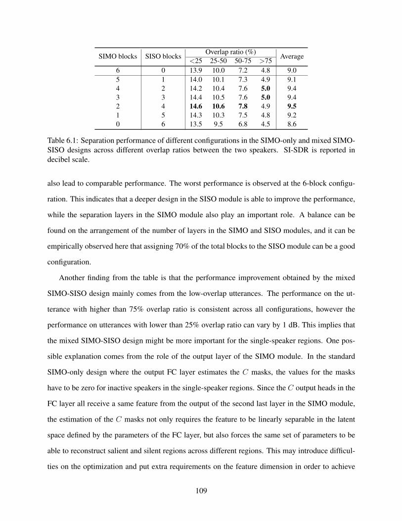
SIMO blocks SISO blocksOverlap ratio (%)

Average<25 25-50 50-75 >75

6 0 13.9 10.0 7.2 4.8 9.05 1 14.0 10.1 7.3 4.9 9.14 2 14.2 10.4 7.6 5.0 9.43 3 14.4 10.5 7.6 5.0 9.42 4 14.6 10.6 7.8 4.9 9.51 5 14.3 10.3 7.5 4.8 9.20 6 13.5 9.5 6.8 4.5 8.6

Table 6.1: Separation performance of different configurations in the SIMO-only and mixed SIMO-SISO designs across different overlap ratios between the two speakers. SI-SDR is reported indecibel scale.

also lead to comparable performance. The worst performance is observed at the 6-block configu-

ration. This indicates that a deeper design in the SISO module is able to improve the performance,

while the separation layers in the SIMO module also play an important role. A balance can be

found on the arrangement of the number of layers in the SIMO and SISO modules, and it can be

empirically observed here that assigning 70% of the total blocks to the SISO module can be a good

configuration.

Another finding from the table is that the performance improvement obtained by the mixed

SIMO-SISO design mainly comes from the low-overlap utterances. The performance on the ut-

terance with higher than 75% overlap ratio is consistent across all configurations, however the

performance on utterances with lower than 25% overlap ratio can vary by 1 dB. This implies that

the mixed SIMO-SISO design might be more important for the single-speaker regions. One pos-

sible explanation comes from the role of the output layer of the SIMO module. In the standard

SIMO-only design where the output FC layer estimates the C masks, the values for the masks

have to be zero for inactive speakers in the single-speaker regions. Since the C output heads in the

FC layer all receive a same feature from the output of the second last layer in the SIMO module,

the estimation of the C masks not only requires the feature to be linearly separable in the latent

space defined by the parameters of the FC layer, but also forces the same set of parameters to be

able to reconstruct salient and silent regions across different regions. This may introduce difficul-

ties on the optimization and put extra requirements on the feature dimension in order to achieve

109

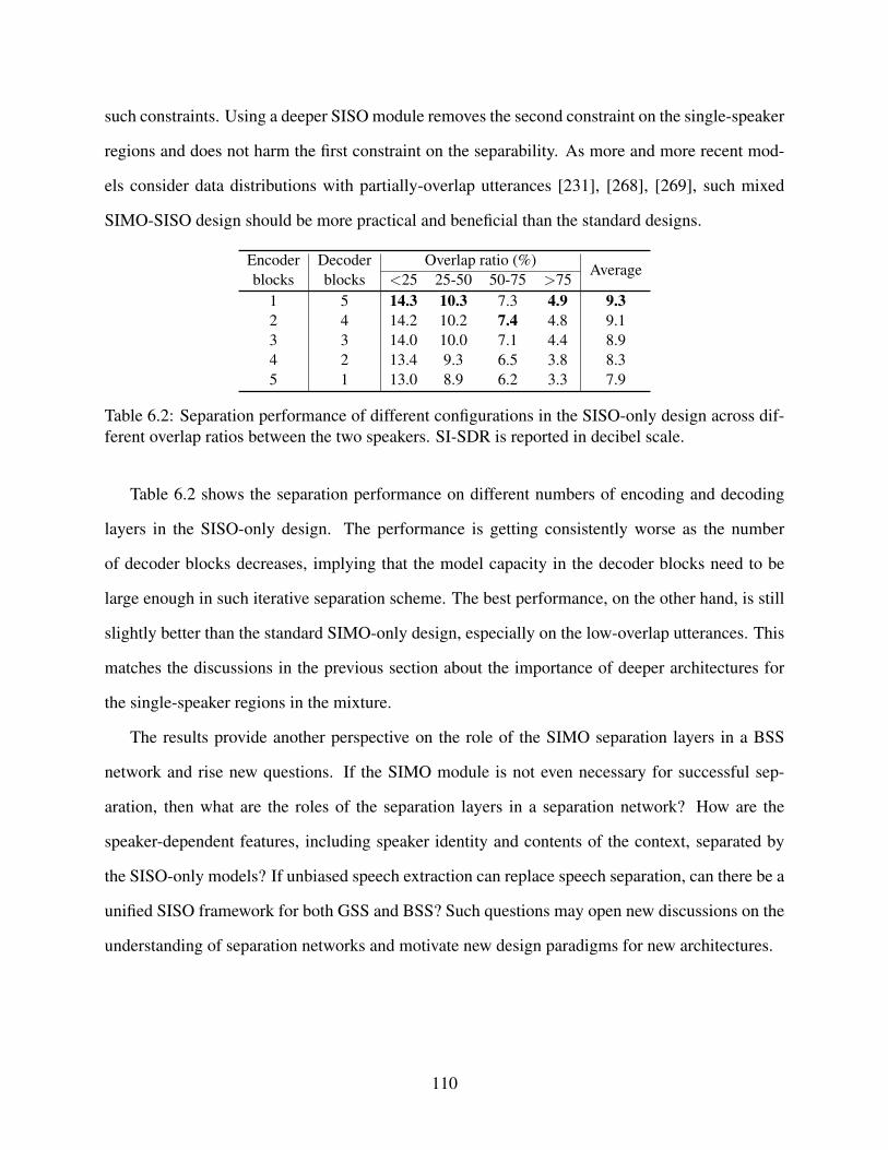
such constraints. Using a deeper SISO module removes the second constraint on the single-speaker

regions and does not harm the first constraint on the separability. As more and more recent mod-

els consider data distributions with partially-overlap utterances [231], [268], [269], such mixed

SIMO-SISO design should be more practical and beneficial than the standard designs.

Encoder Decoder Overlap ratio (%)Average

blocks blocks <25 25-50 50-75 >751 5 14.3 10.3 7.3 4.9 9.32 4 14.2 10.2 7.4 4.8 9.13 3 14.0 10.0 7.1 4.4 8.94 2 13.4 9.3 6.5 3.8 8.35 1 13.0 8.9 6.2 3.3 7.9

Table 6.2: Separation performance of different configurations in the SISO-only design across dif-ferent overlap ratios between the two speakers. SI-SDR is reported in decibel scale.

Table 6.2 shows the separation performance on different numbers of encoding and decoding

layers in the SISO-only design. The performance is getting consistently worse as the number

of decoder blocks decreases, implying that the model capacity in the decoder blocks need to be

large enough in such iterative separation scheme. The best performance, on the other hand, is still

slightly better than the standard SIMO-only design, especially on the low-overlap utterances. This

matches the discussions in the previous section about the importance of deeper architectures for

the single-speaker regions in the mixture.

The results provide another perspective on the role of the SIMO separation layers in a BSS

network and rise new questions. If the SIMO module is not even necessary for successful sep-

aration, then what are the roles of the separation layers in a separation network? How are the

speaker-dependent features, including speaker identity and contents of the context, separated by

the SISO-only models? If unbiased speech extraction can replace speech separation, can there be a

unified SISO framework for both GSS and BSS? Such questions may open new discussions on the

understanding of separation networks and motivate new design paradigms for new architectures.

110

6.2 Empirical Analysis of Generalized Iterative Speech Separation Networks


The design of a wide range of speech separation networks follows a general one-pass pipeline,

where the input mixture waveform is passed to a neural network to directly estimate the target

sources [80], [121], [173], [187], [201], [243]. On the other hand, recent developments on the

multi-pass or iterative pipeline have shown improved separation performance [123], [148], [234],

[253], [306]. Conventional iterative separation pipelines were typically designed by certain it-

erative algorithms, such as Expectation-Maximization (EM) and nonnegative matrix factorization

(NMF) [49], [105], [169], where multiple iterations are required for the algorithms to converge and

achieve a satisfying performance. In neural network-based systems, an iterative speech separation

pipeline can be defined as a system that contains multiple rounds of the separation process, where

(1) each iteration performs a full separation pipeline, and (2) the separation outputs from a previous

iteration can be used as additional information in an upcoming iteration. In single-channel appli-

cations, the iterative pipeline has proven better than one-pass pipelines with comparable model

complexity [234], [306]. In multi-channel applications, the iterative pipeline can improve the per-

formance of either a vocal activity detector (VAD) or a beamformer [183], [253], [333]. Different

features such as speaker-specific embeddings can also be extracted from the previous separation

outputs and serve as the additional feature for following iterations [216], [254], [307], [313].

A common configuration for such iterative separation pipeline is that the training objective,

typically the discrepancy between the estimated and target sources, is applied to all the iterations.

By unfolding the iterations into additional layers or modules in a deeper network, such training

objective corresponds to a layer-wise objective in one-pass pipelines [293], [303]. Moreover, the

objective can be further extended to models where a post-enhancement stage is applied to each of

the separation outputs [118], [148], [171], [241], [272]. This gives a generalized iterative separa-

tion pipeline where the same training objective is applied to different parts of the network. Differ-

ent model design and architecture configurations in such generalized iterative separation pipelines

111

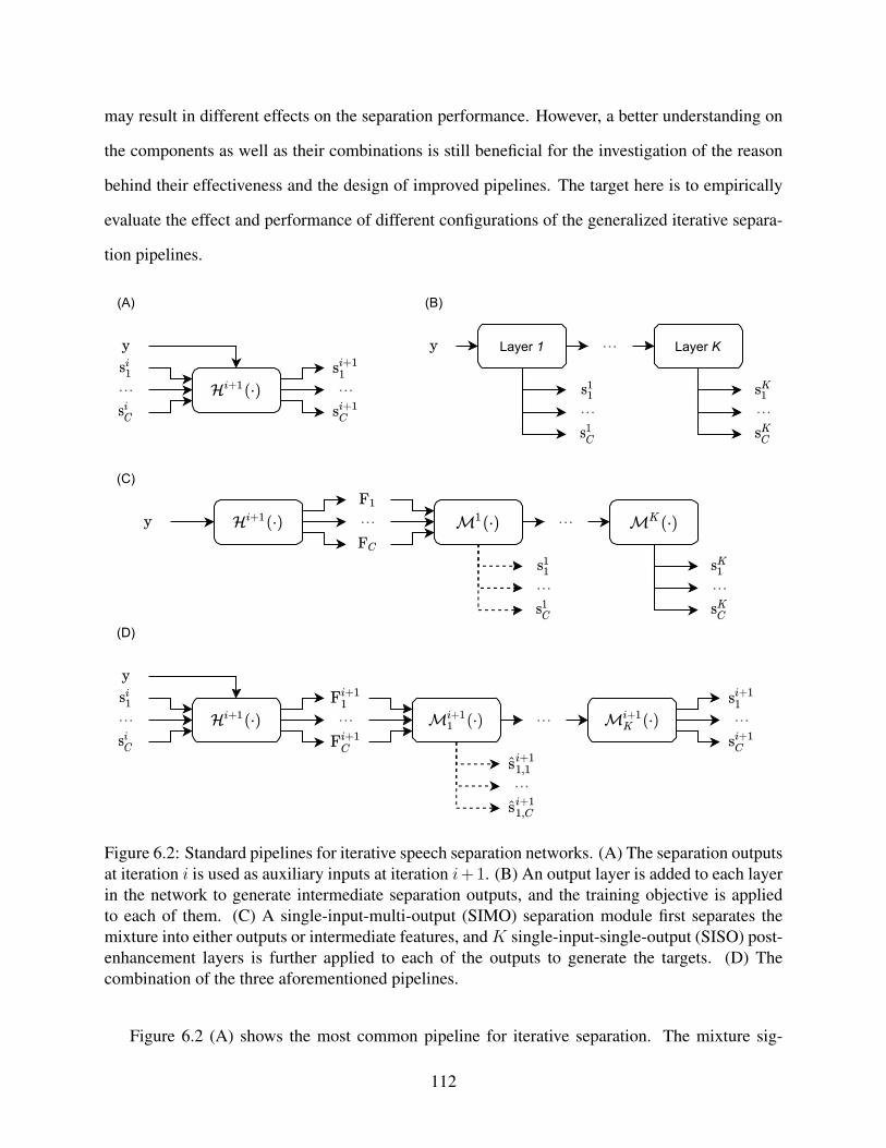
may result in different effects on the separation performance. However, a better understanding on

the components as well as their combinations is still beneficial for the investigation of the reason

behind their effectiveness and the design of improved pipelines. The target here is to empirically

evaluate the effect and performance of different configurations of the generalized iterative separa-

tion pipelines.

···

Layer 1

···

Layer K···

··· ···

··· ···

··· ···

(A) (B)

(C)

······ ··· ···

···

(D)

Figure 6.2: Standard pipelines for iterative speech separation networks. (A) The separation outputsat iteration i is used as auxiliary inputs at iteration i+ 1. (B) An output layer is added to each layerin the network to generate intermediate separation outputs, and the training objective is appliedto each of them. (C) A single-input-multi-output (SIMO) separation module first separates themixture into either outputs or intermediate features, and K single-input-single-output (SISO) post-enhancement layers is further applied to each of the outputs to generate the targets. (D) Thecombination of the three aforementioned pipelines.

Figure 6.2 (A) shows the most common pipeline for iterative separation. The mixture sig-

112

nal y, together with the separation output from i-th iteration {sic}Cc=1, is passed to the (i + 1)-th

single-input-multi-output (SIMO) mapping H(i+1)(·) defined by a neural network, to generate the

separation outputs at the (i+1)-th iteration {si+1c }Cc=1. For the first iteration, {s0

c}Cc=1 are initialized

as zero signals. The output permutation at the i-th iteration is used as the input permutation at the

(i+ 1)− th iteration, and empirically this can maintain the output permutation across all iterations

without affecting the separation performance.

There are two optional designs in this pipeline. First, the model parameters across different

iterations can be either shared or different. This can be related to the general definition of time-

invariant and time-variant systems. Second, when performing backpropagation, the gradient of the

input to the (i+1)-th iteration can either pass to the i-th iteration or be discarded. In the latter case,

each iteration can be viewed as an independent process, and the output from the previous iteration

can be treated as additional bias information for data augmentation.

Figure 6.2 (B) shows a typical generalized iterative separation pipeline where the training ob-

jective is applied to all the layers in the separator. For the k-th layer where K = 1, . . . , K, a

shared output layer is applied to its output to generate intermediate separation outputs {skc}Cc=1.

The pipeline is defined as a generalized iterative separation network because all layers in the sepa-

rator are directly optimized with the same training objective to minimize the discrepancy between

the (intermediate) separation outputs and the target sources, hence layer k with k ≥ 2 can be

treated as iterative separation layers receiving separation outputs from layer k − 1. This is unlike

the standard pipeline where the training objective is only applied to the output at layer K and the

outputs at other layers do not have a clear and explicit meaning.

Figure 6.2 (C) shows the pipeline with a pre-separation module and a post-enhancement mod-

ule. The pre-separation module receives the mixture as input and generates C outputs {Fc}Cc=1

for the C target sources. Note that {Fc}Cc=1 can either be intermediate features or the estimated

targets themselves. Each feature Fc is then passed to a post-enhancement module with K SISO

layers for output refinement, and the separation outputs can be generated from either each SISO

layer (i.e., layer-wise objective) or the last SISO layer only. It is defined as a generalized iterative

113

separation pipeline when the training objective is applied to each of the post-enhancement lay-

ers. Moreover, the training objective can also be applied to {Fc}Cc=1 when they correspond to the

separation outputs.

Figure 6.2 (D) shows a combined pipeline for the three pipelines above. The separation-

enhancement pipeline is inserted into the standard iterative pipeline, where the SISO enhancement

layers together with optional layer-wise objectives are jointly applied together with the SIMO sep-

aration module. The outputs at the k-th SISO enhancement layer at the (i+ 1)-th iteration become

{si+1k,c }Cc=1.

For the experiments, the combined pipeline is used following the same architecture in Chap-

ter 6.1. Both time-domain and frequency-domain models are evaluated by selecting either learn-

able encoder and decoder or short-time Fourier transform (STFT) and its inverse (ISTFT). For

STFT/ISTFT, only the magnitude spectrogram is used as the input, and the mixture’s phase spec-

trogram is directly used for the ISTFT of the separation outputs. The window size for the learn-

able encoder/decoder and STFT/ISTFT is set to 2 ms (32 points) and 32 ms (512 points), respec-

tively. The number of filters in the encoder and decoder for the learnable encoder/decoder and

STFT/ISTFT is set to 128 and 257, respectively. A linear bottleneck layer with 64 hidden units is

always applied to the encoder output for dimension reduction. The number of hidden units in each

of the LSTM layers in the DPRNN modules is set to 128. The segment size for DPRNN is set to

100 frames and 24 frames for the learnable encoder/decoder and STFT/ISTFT, respectively.


Table 6.3: Experiment results for different configurations in the iterative separation pipeline.

SIMO layers SISO layers Iteration Effective network depth Output detach SI-SDR (dB)Time domain Freq domain

3 01 3 –

8.7 8.42 1 9.0 8.71 2 9.2 9.1

1 2 2 63 9.8 9.67 9.7 9.5

2 4 1 – 10.0 9.5

1 2 3 93 10.1 9.87 9.6 9.5

3 6 1 – 10.2 9.4

114

Table 6.3 shows the experiment results of the networks with different configurations. The

model parameters are assumed shared across all iterations in the models. Each SIMO and SISO

layer corresponds to a DPRNN block, and 0 SISO layers means that the output of the SIMO layers

are the separation outputs. First notice that for both time-domain and frequency-domain models,

a deeper SISO module leads to better performance. Since Chapter 6.1 already showed that a deep

SISO module improves the performance of time-domain networks, here the results further confirm

that frequency-domain networks can also benefit from this configuration. For iterative networks

with the number of iterations larger than 1, they are also compared with one-pass models with a

same effective network depth. The “output detach” column corresponds to the configuration where

the gradient is constrained within each iteration (which can be implemented by detach function in

Pytorch or stop_gradient function in Tensorflow). It can be observed that for the 2-iteration con-

figuration, both time-domain and frequency-domain models have comparable performance with

their corresponding one-pass models. Moreover, detaching the gradient from the previous output

leads to a minor improvement. For the 3-iteration configuration, the improvement introduced by

gradient detachment becomes more salient, and the frequency-domain model even outperform the

one-pass counterpart. The results here show that the iterative separation pipeline can serve as an

effective way to reduce the storage requirement of the separation networks.

Table 6.4: Effect of layer-wise training objective.

SIMO layers SISO layers Iteration SI-SDR (dB)Time domain Freq domain

1 2 3 9.9 9.43 6 1 10.1 9.2

Table 6.4 provides the separation performance of the iterative systems with layer-wise training

objective. The output at each SISO layer in each iteration is passed to the shared mask estimation

layer to generate the separated waveforms, and the negative SNR objective is applied to all out-

puts in the entire pipeline. The configuration where output detachment is applied and parameters

are shared across iterations is selected here. Comparing the results with the ones in Table 6.3,

layer-wise objective does not further improve the performance in either one-pass or iterative con-

figurations. [293] and [303] reported that layer-wise objective leads to a performance improvement

115

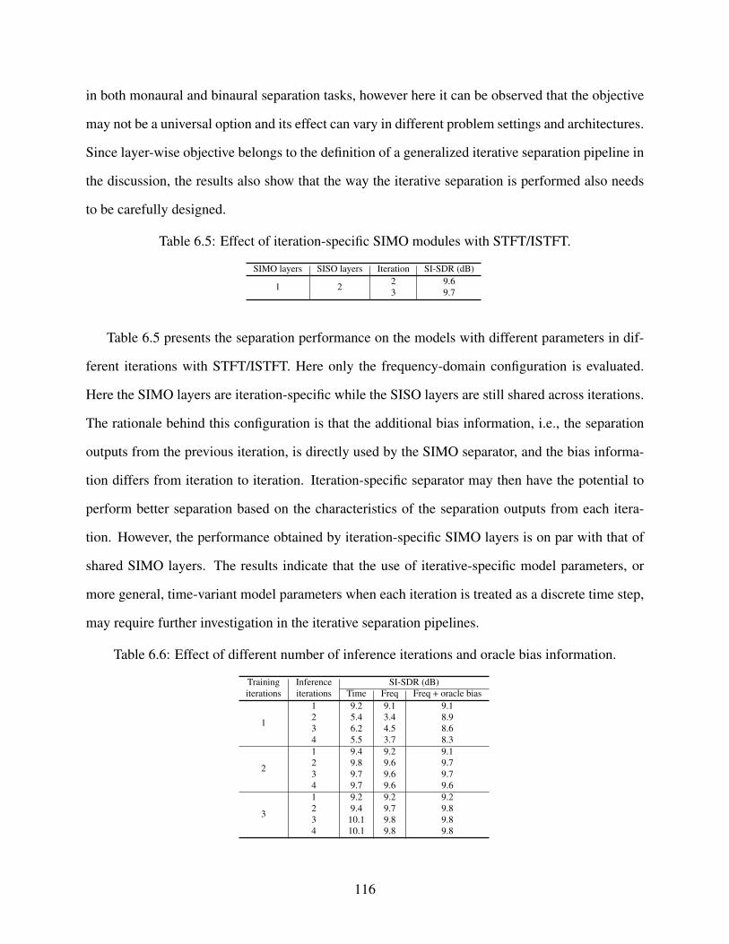
in both monaural and binaural separation tasks, however here it can be observed that the objective

may not be a universal option and its effect can vary in different problem settings and architectures.

Since layer-wise objective belongs to the definition of a generalized iterative separation pipeline in

the discussion, the results also show that the way the iterative separation is performed also needs

to be carefully designed.

Table 6.5: Effect of iteration-specific SIMO modules with STFT/ISTFT.

SIMO layers SISO layers Iteration SI-SDR (dB)

1 2 2 9.63 9.7

Table 6.5 presents the separation performance on the models with different parameters in dif-

ferent iterations with STFT/ISTFT. Here only the frequency-domain configuration is evaluated.

Here the SIMO layers are iteration-specific while the SISO layers are still shared across iterations.

The rationale behind this configuration is that the additional bias information, i.e., the separation

outputs from the previous iteration, is directly used by the SIMO separator, and the bias informa-

tion differs from iteration to iteration. Iteration-specific separator may then have the potential to

perform better separation based on the characteristics of the separation outputs from each itera-

tion. However, the performance obtained by iteration-specific SIMO layers is on par with that of

shared SIMO layers. The results indicate that the use of iterative-specific model parameters, or

more general, time-variant model parameters when each iteration is treated as a discrete time step,

may require further investigation in the iterative separation pipelines.

Table 6.6: Effect of different number of inference iterations and oracle bias information.

Training Inference SI-SDR (dB)iterations iterations Time Freq Freq + oracle bias

1

1 9.2 9.1 9.12 5.4 3.4 8.93 6.2 4.5 8.64 5.5 3.7 8.3

2

1 9.4 9.2 9.12 9.8 9.6 9.73 9.7 9.6 9.74 9.7 9.6 9.6

3

1 9.2 9.2 9.22 9.4 9.7 9.83 10.1 9.8 9.84 10.1 9.8 9.8

116

Table 6.6 measures the effect of different inference iterations. For the models trained with 1,

2, and 3 iterations with 1 SIMO layer and 2 SISO layers, their performance is evaluated with 1

to 4 iterations in the inference phase. This experiment is conducted to look into the effect of a

mismatched number of iterations on the training and inference phases. It can be observed that

the model trained with 1 iteration completely fails when more than 1 iteration is applied in the

inference phase, which is expected since the bias information starting from the second iteration

is completely unseen for the SIMO separation. When the model is trained for no fewer than 2

iterations, the inference phase performance becomes stable even if the inference phase iteration is

larger than the training phase iteration. Moreover, the evaluation is done on the performance of the

frequency-domain model when the oracle bias information, i.e., the clean target sources, is used for

the SIMO module, and an auxiliary training objective is added to the overall training objectives.

Adding this oracle bias information allows the model trained with 1 iteration to perform much

better in inference phase and does not harm the performance of the models trained with 2 and 3

iterations. However, no obvious performance improvement is achieved by the auxiliary loss. How

to further improve the separation performance of those iterative models remains an important topic

to explore.

6.3 Empirical Analysis of the Effect of Separation Network Components under a Time-

domain Training Objective


Different configurations can be adjusted in the three components of a typical end-to-end speech

separation system: an encoder, a separator, and a decoder. On the one hand, short-time Fourier

transform (STFT) and its inverse can also be seamlessly incorporated to the end-to-end training

pipelines [226], [234]. On the other hand, the output of the separator can either be a set of multi-

plicative masks applied to the mixture’s latent representation, or the target sources’ latent represen-

tations that can be directly decoded. These two types of outputs match to masking-based configura-

tion and the regression-based configuration. It has been shown that regression-based configuration

117

can be beneficial than masking-based configuration in various problem settings [266], [293]. The

target here is to empirically revisit the effect of different combinations of the component-level

configurations on the separation performance.

SIMO modules

SISO modules

Linear bottleneck

Encoder (Learnable / STFT)

Decoder (Learnable / ISTFT)··· ··· ···Linear

bottleneckMixture

Source 1

Source C

···

Figure 6.3: Flowchart for a standard speech separation pipeline. An encoder first transforms themixture into a latent representation, and a linear bottleneck layer reduces its dimension. A single-input-multi-output (SIMO) separation module generates C features correspond to the C targetsources. Each output is concatenated with the encoder output and passed to another linear bot-tleneck layer for dimension reduction, and a single-input-single-output (SISO) module is appliedto estimate either a multiplicative mask for the encoder output or the latent representation for thetarget source directly. A decoder is finally used to reconstruct the target waveforms.

Figure 6.3 shows the general pipeline for an end-to-end speech separation system, which is

identical to the pipeline introduced in Chapter 2. An encoder first transforms the mixture wave-

form into a latent representation. A layer normalization operation [114] is then applied on the

representation, and a linear bottleneck layer reduces the feature dimension of the representation.

The feature is then sent to a single-input-multi-output (SIMO) module to generate 2 outputs. Each

of the outputs is then concatenated with the normalized mixture latent representation and sent to

another linear bottleneck layer for dimension reduction, and a single-input-single-output (SISO)

module follows to estimate either a multiplicative mask applied to the mixture’s latent represen-

tation or the latent representation of the target signals directly. A decoder is finally applied to

reconstruct the target waveforms.

Within the DPRNN-TasNet framework, different configurations of the pipeline are evaluated:

1. Encoder/Decoder: Both learnable encoder/decoder and STFT/ISTFT can be used. For learn-

able encoder/decoder, 1-D linear convolutional/transposed-convolutional layers identical to

the ones in Chapter 2.2 are used. For STFT/ISTFT, either the magnitude spectrogram (i.e.,

mag-spec configuration) or the concatenation of real and imaginary parts of the complex-

118

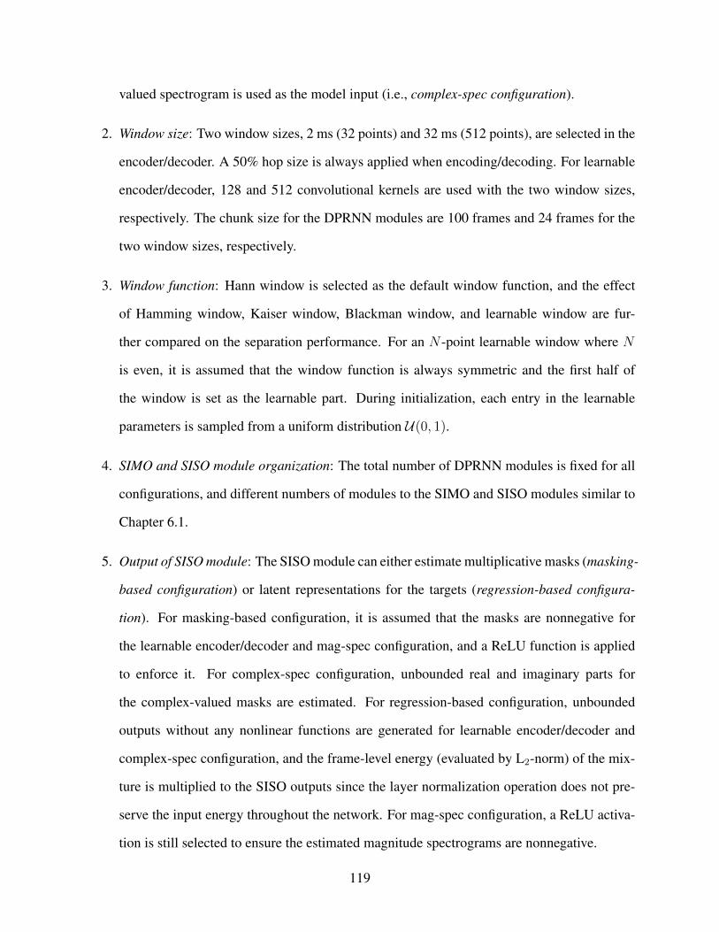
valued spectrogram is used as the model input (i.e., complex-spec configuration).

2. Window size: Two window sizes, 2 ms (32 points) and 32 ms (512 points), are selected in the

encoder/decoder. A 50% hop size is always applied when encoding/decoding. For learnable

encoder/decoder, 128 and 512 convolutional kernels are used with the two window sizes,

respectively. The chunk size for the DPRNN modules are 100 frames and 24 frames for the

two window sizes, respectively.

3. Window function: Hann window is selected as the default window function, and the effect

of Hamming window, Kaiser window, Blackman window, and learnable window are fur-

ther compared on the separation performance. For an N -point learnable window where N

is even, it is assumed that the window function is always symmetric and the first half of

the window is set as the learnable part. During initialization, each entry in the learnable

parameters is sampled from a uniform distribution U(0, 1).

4. SIMO and SISO module organization: The total number of DPRNN modules is fixed for all

configurations, and different numbers of modules to the SIMO and SISO modules similar to

Chapter 6.1.

5. Output of SISO module: The SISO module can either estimate multiplicative masks (masking-

based configuration) or latent representations for the targets (regression-based configura-

tion). For masking-based configuration, it is assumed that the masks are nonnegative for

the learnable encoder/decoder and mag-spec configuration, and a ReLU function is applied

to enforce it. For complex-spec configuration, unbounded real and imaginary parts for

the complex-valued masks are estimated. For regression-based configuration, unbounded

outputs without any nonlinear functions are generated for learnable encoder/decoder and

complex-spec configuration, and the frame-level energy (evaluated by L2-norm) of the mix-

ture is multiplied to the SISO outputs since the layer normalization operation does not pre-

serve the input energy throughout the network. For mag-spec configuration, a ReLU activa-

tion is still selected to ensure the estimated magnitude spectrograms are nonnegative.

119

Beyond the configurations above, the encoder bottleneck layer and the SISO bottleneck layer

always contain 64 hidden units, and each LSTM in the DPRNN modules always has 128 hidden

units.


Table 6.7, 6.8 and 6.9 provide the separation performance of models with different pipeline con-

figurations. The experiments are first conducted with the total number of DPRNN modules fixed to

3, and then the model sizes are doubled for the best organizations. For learnable encoder/decoder

configuration, regression-based configuration leads to better performance than masking-based con-

figuration with 2 ms window, and the performance improves as the number of SISO layers in-

creases. Moreover, increasing the total model size further improves the separation performance

in both configurations. However, masking-based configuration performs consistently better than

regression-based configuration with 32 ms window, and the performance does not increase with a

larger network size. For the mag-spec configuration, the performance of both masking-based and

regression-based configurations are stable across the two window sizes, while masking-based con-

figuration prefers a larger window and regression-based configuration prefers a smaller window.

The best performance is also achieved by the masking-based configuration with 32 ms window,

which is similar to the best performance in learnable encoder/decoder configuration with a much

lower model complexity due to the use of a larger window size. For the complex-spec config-

uration, a similar overall performance as the learnable encoder/decoder can be observed, while

the performance for masking-based configuration is slightly higher. The best performance is still

achieved by regression-based configuration with 2 ms window, but it is still slightly worse than

that with learnable encoder/decoder.

Then the necessity of the nonnegativity constraint in magnitude T-F masks is revisited. The

ReLU nonlinearity in the output layer is removed and the performance of unbounded magnitude

masks is evaluated. Table 6.10 shows that the performance of nonnegative masks and unbounded

masks has little or no difference in different model and window sizes, which indicates that the

120

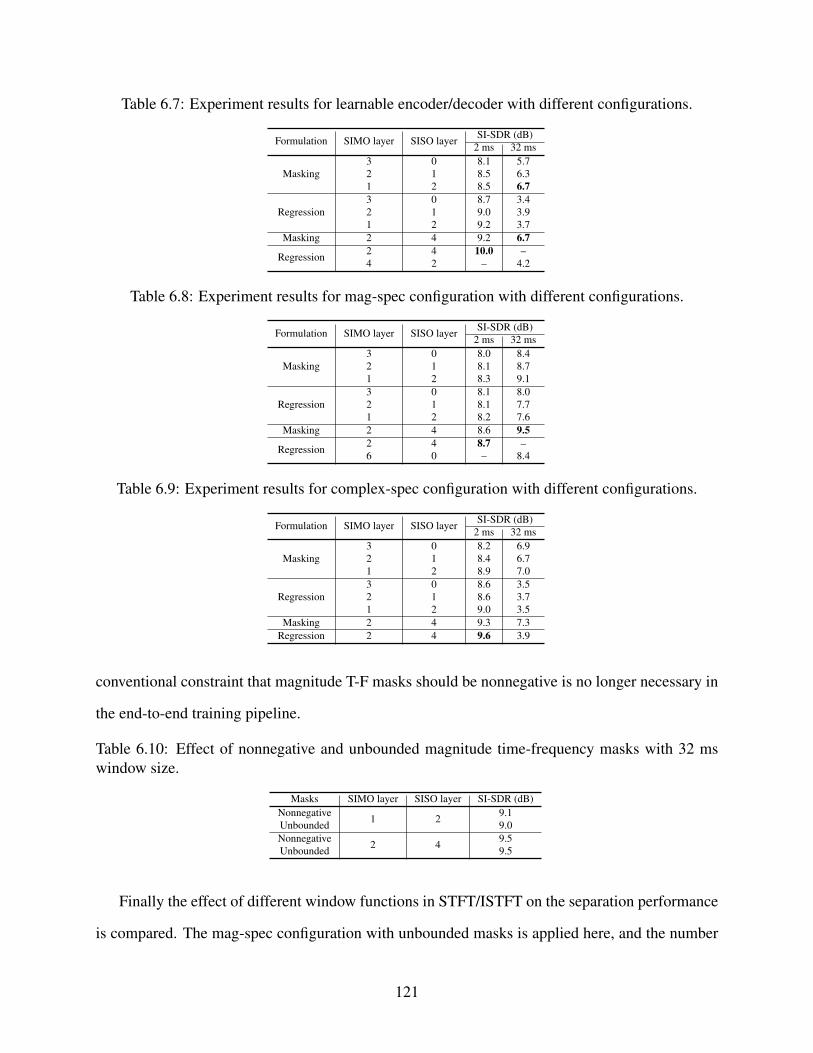
Table 6.7: Experiment results for learnable encoder/decoder with different configurations.

Formulation SIMO layer SISO layer SI-SDR (dB)2 ms 32 ms

Masking3 0 8.1 5.72 1 8.5 6.31 2 8.5 6.7

Regression3 0 8.7 3.42 1 9.0 3.91 2 9.2 3.7

Masking 2 4 9.2 6.7

Regression 2 4 10.0 –4 2 – 4.2

Table 6.8: Experiment results for mag-spec configuration with different configurations.


Masking3 0 8.0 8.42 1 8.1 8.71 2 8.3 9.1

Regression3 0 8.1 8.02 1 8.1 7.71 2 8.2 7.6

Masking 2 4 8.6 9.5

Regression 2 4 8.7 –6 0 – 8.4

Table 6.9: Experiment results for complex-spec configuration with different configurations.


Masking3 0 8.2 6.92 1 8.4 6.71 2 8.9 7.0

Regression3 0 8.6 3.52 1 8.6 3.71 2 9.0 3.5

Masking 2 4 9.3 7.3Regression 2 4 9.6 3.9

conventional constraint that magnitude T-F masks should be nonnegative is no longer necessary in

the end-to-end training pipeline.

Table 6.10: Effect of nonnegative and unbounded magnitude time-frequency masks with 32 mswindow size.

Masks SIMO layer SISO layer SI-SDR (dB)Nonnegative 1 2 9.1Unbounded 9.0Nonnegative 2 4 9.5Unbounded 9.5

Finally the effect of different window functions in STFT/ISTFT on the separation performance

is compared. The mag-spec configuration with unbounded masks is applied here, and the number

121

of SIMO and SISO DPRNN layers are set to 1 and 2, respectively, according to the best config-

urations above. It can be observed that the choice of window function does affect the separation

performance, while the model without a window function has the worst performance. Interestingly,

the learnable window function achieves a relatively better performance comparing with all other

well-defined window functions even with a random initialization. Figure 6.4 visualizes the learned

window function and its frequency response.

Table 6.11: Effect of window functions in mag-spec configuration with unbounded magnitude T-Fmasks and 32 ms window size.

Window SI-SDR (dB)None 8.5Hann 9.0

Hamming 9.1Kaiser 8.6

Blackman 8.8Learnable 9.2

Figure 6.4: Visualization of the learned window function and its frequency response.

Multiple analysis and discussions can be made based on the results above:

1. It can be found from the results that proper organizations of SIMO and SISO modules can

improve the separation performance in both masking-based and regression-based config-

urations. This matches the observation in Chapter 6.1. Moreover, the SISO module can

122

be considered as a neural vocoder jointly optimized with the separator in regression-based

configurations, which builds connections to the recent works on synthesis-based speech en-

hancement and separation methods [244], [266], [271], [292].

2. Compare the performance of masking-based configuration between learnable encoder/decoder

and complex-spec configurations, the performance of complex-spec configuration is consis-

tently better than the learnable encoder/decoder across both window sizes. Since the main

differences between the complex-spec configuration and the learanble encoder/decoder are

the use of fixed orthogonal basis kernels (i.e., sinusoids) and the minimum mean-square error

(MMSE) estimation of the waveform in ISTFT [4], it implies that domain-specific knowl-

edge can still be beneficial in the design of encoder and decoder. Moreover, the performance

in small window size is significantly better than that in large window size, which matches

the observation in previous studies [234], [287].

3. In contrast to the results above, the performance of mag-spec configuration with large win-

dow is better than that with small window. Moreover, its performance in large window is

also better than the complex-spec configuration. Since the phase spectrogram is unmodi-

fied in this pipeline, it becomes more interesting to investigate the role phase information

in masking-based pipelines. It has been shown in other literature that T-F domain training

objectives can be successfully applied with complex-valued input and outputs [133], [239],

[308], hence it is necessary to learn more about the behavior of STFT/ISTFT representa-

tions with a time-domain objective. The conventional definition of magnitude T-F masks

also needs to be reconsidered, as in end-to-end pipelines the ISTFT process as well as the

overlap-add operation for waveform reconstruction both contributes to the backpropagation

process and can greatly change the behavior of magnitude T-F masks. As an evidence,

unbounded magnitude masks achieve same performance as nonnegative magnitude masks.

Note that since a negative-valued mask corresponds to a phase shift of π as −eiθ = ei(θ+π),

such unbounded masks can be viewed as constrained complex-valued masks where the phase

123

at each T-F bin can be modified by either 0 degree or 180 degree. These results indicate that

the conventional definition and analysis of T-F masks needs a revision in the end-to-end

pipeline, and the role and effect of T-F masking needs to be reconsidered.

4. One core advantage for regression-based configuration is that it bypasses the issue in masking-

based configuration which binds the separation outputs with the mixture’s encoder output. It

can be observed that regression-based configuration performs consistently better in a smaller

window than a larger window, and the best system across all possible configurations (10.0

dB SI-SDR) is achieved by the regression-based configuration with a small window size.

This shows that when properly configured, regression-based configuration has the potential

to outperform masking-based configuration. This matches the conclusion in a prior work

[266].

5. The performance comparison on different encoder/decode types gives a mixed conclusion.

On the one hand, both learnable encoder/decoder and complex-spec configurations use a

phase information different than the mixture phase during reconstruction, which confirms

that the ability for accurate phase reconstruction can lead towards a better separation per-

formance. On the other hand, the performance gap between small and large windows in

those two encoder/decoder configurations is significantly larger than that in mag-spec con-

figuration, which implies again that it is not always beneficial to modify the phase when

a large window is selected. Another observation is that the performance of learnable en-

coder/decoder and the complex-spec configuration is comparable across all experiments.

This also implies that the actual choice of kernel parameters in the learnable encoder/decoder

might not be an important factor, especially in the regression-based configuration where the

output waveforms are directly generated.

6. [264] has considered trainable STFT window functions in the speech enhancement task.

However, it used different window functions for STFT and ISTFT without symmetric con-

straint and applied a frequency-domain training objective, and did not compare the perfor-

124

mance with different types of existing window functions. Here it is further confirmed that

the choice of window function is indeed a factor that can be optimized, and certain window

functions may not even be helpful (e.g., the Kaiser window). Moreover, it is showed that the

learned window function does “look like” a standard window function with random initial-

ization and without a nonnegativity constraint. It is obvious that its frequency response is not

ideal comparing with other well-defined window functions such as the Hann or Hamming

windows, however it achieves a slightly better performance than any other windows. This

also serves as a proof showing that the behavior of STFT/ISTFT can be complicated in the

end-to-end training pipeline.

125

Conclusion and Future Works

This dissertation focused on advancing the state-of-the-art methods on the problem of speech

separation with neural networks. The contributions of this dissertation can be categorized into

three classes: problem formulations, network architectures, and training objectives.

1. Problem formulations: The formulation of end-to-end speech separation in time domain

was proposed and validated. STFT and its inverse were replaced by real-valued, learnable

1-D convolutional and transposed convolutional layers, and time-domain training objectives

were applied to directly optimize the evaluation metrics. In the single-channel scenario, the

TasNet framework introduced in Chapter 2 has achieved higher performance than multiple

oracle T-F masks and has become a benchmark in the general problem of speech separation.

In the multi-channel scenario, the FaSNet framework introduced in Chapter 3 has achieved

superior performance compared to multiple oracle beamformers in terms of signal quality

measures. Moreover, by revisiting the commonly-used model configurations for speech

separation in Chapter 6, additional questions were raised for a better understanding on the

intrinsic mechanisms of the end-to-end speech separation pipelines.

2. Network architectures: Multiple network architectures were proposed to not only improve

the separation performance but also decrease the model complexity. The TCN and DPRNN

architectures introduced in Chapter 2 have been widely adopted in the community, and the

GC3 architecture introduced in Chapter 4 has the potential to become a general design

paradigm in low-resource platforms and applications.

126

3. Training objectives: Training objectives were proposed in Chapter 5 to improve the

robustness of the separation networks under reverberation and to allow the systems to

separate arbitrary numbers of sources with a single model. Both of the proposed training

objectives, A2T and A2PIT, utilized the idea of auxiliary autoencoding loss, and a

modification to the commonly-used SI-SDR and SNR functions were also proposed to

control the range of the gradients when the auxiliary autoencoding loss was applied.

There remains many interesting problems in the general context of speech separation to solve:

1. Separation of unsegmented speech: The systems introduced in this dissertation were all

evaluated on utterance-level datasets, where the length of the mixtures are typically small

than 10 seconds. Real-world communications often involve unsegmented speech with

time-varying characteristics of speaker overlaps, speaker locations, and speaker activations.

How to properly perform speech separation in such long recordings is a critical problem for

the deployment of speech separation systems to real-world applications such as meeting

transcription systems. Recent studies have started investigating this direction [267], [268],

[275], [309], [321], [322], [328], [331], [332], and it is expected that the development of the

systems on this task can be accelerated when more realistic meeting-style data with

multiple overlapped speakers is collected and released [330].

2. Separation under strong reverberation: Although the A2T training objective was proposed

to improve the system robustness under reverberation, it did not significantly improve the

overall separation performance in terms of signal quality. It is unclear whether time-domain

training objectives such as SNR and SI-SDR are still good training objectives under strong

reverberation, since such objectives do not consider frequency-dependent properties of the

sources and are highly phase-sensitive. Recent works have attempted to propose new

time-domain training objectives for reverberant speech separation [263], while the proposed

function has the same drawback as the SDR metric introduced in Chapter 1.3. On the other

hand, current model architectures for reverberant speech separation are almost always

127

identical to the ones for anechoic speech separation, and new model architectures that better

reflect the properties of the reverberant signals may be beneficial in this task. It it thus

worth exploring new training objectives and model architectures for this problem.

3. Separation with preserved spatial cues: Spatial cues are important features that allow

human beings to precisely perceive the spatial location of the sound sources. Preserving the

spatial cues during separation can result in a more realistic hearing experience in either

real-world or virtual environments. Recent works have started to investigate this problem

with different neural network architectures on various artificially simulated binaural speech

datasets [276], [303], [318]. However, the performance of such systems on real-world

conversations with moving sources remains unclear, and whether the existing systems

satisfy the latency and complexity requirements in real-world devices and applications also

needs further verification. Moreover, spatial cues can be hard to accurately measure in

noisy reverberant environments, and how to properly define both the evaluation metrics and

the training objectives of the systems is also an interesting problem.

4. Separation as a front-end: The recognition of overlapped speech can be done by a

multi-talker ASR system without an explicit speech separation model [172], [182], [281],

[317]. However, it is natural to first apply a speech separation model as a front-end module

and use a standard single-channel ASR system as a back-end [139], [206], [209], [227],

[295], [296]. Current pipelines that use a separation model as a front-end still cannot

achieve on-par performance as a plain ASR system trained on clean single-speaker

utterances, and it is important to continue investigating this direction and mitigate the

performance gap.

5. Multi-modal speech separation: The entire dissertation focused on the audio-only speech

separation task. Researchers have also studied the design of multi-modal source separation

models in the audio-visual [186], [257], [274], [327], audio-textual [104], [285], [336], and

audio-motion [158], [301] modalities. There are two main directions to further explore this

128

topic. The first one is to continue developing novel system designs to better connect the

data from different modalities in a joint embedding space, and existing works in

multi-modal data modeling and understanding have shown potentials on it [61], [84], [86],

[128], [329]. The second one is how to alleviate the inconsistency between different

modalities. Consider a meeting-style conversation with speakers moving their heads while

talking. A camera may miss the location of the speaker’s face, and a sound localization

module may generate rapidly changing DOA information with a moving head. A separation

system that relies on these two features may easily get confused when the face information

is lost or when the DOA information has a clear mismatch with the location of the face.

How to ensure the robustness of the multi-modal system with such inaccurate or even

inconsistent features is an important topic for practical applications.

6. A theoretical understanding on end-to-end separation: Chapter 6 has empirically analyzed

the effect of different model configurations with a time-domain training objective. It is

natural to further explore a theoretical understanding on the behaviors of the models,

especially on the role of different encoder and decoder configurations in the entire

separation pipelines.

129

References

[1] R. R. Sokal, “A statistical method for evaluating systematic relationship,” University ofKansas science bulletin, vol. 28, pp. 1409–1438, 1958.

[2] C. Knapp and G. Carter, “The generalized correlation method for estimation of time delay,”IEEE/ACM Transactions on Audio, Speech, and Language Processing (TASLP), vol. 24,no. 4, pp. 320–327, 1976.

[3] J. B. Allen and D. A. Berkley, “Image method for efficiently simulating small-room acous-tics,” The Journal of the Acoustical Society of America, vol. 65, no. 4, pp. 943–950, 1979.

[4] D. Griffin and J. Lim, “Signal estimation from modified short-time fourier transform,”IEEE Transactions on Acoustics, Speech, and Signal Processing, vol. 32, no. 2, pp. 236–243, 1984.

[5] R. Mucci, “A comparison of efficient beamforming algorithms,” IEEE/ACM Transactionson Audio, Speech, and Language Processing (TASLP), vol. 32, no. 3, pp. 548–558, 1984.

[6] J. C. Platt and A. H. Barr, “Constrained differential optimization,” in Neural InformationProcessing Systems, 1988, pp. 612–621.

[7] B. D. Van Veen and K. M. Buckley, “Beamforming: A versatile approach to spatial filter-ing,” IEEE assp magazine, vol. 5, no. 2, pp. 4–24, 1988.

[8] J. S. Garofolo, L. F. Lamel, W. M. Fisher, J. G. Fiscus, and D. S. Pallett, “Timit acoustic-phonetic continous speech corpus cd-rom. nist speech disc 1-1.1,” NASA STI/Recon tech-nical report n, vol. 93, 1993.

[9] G. J. Brown and M. Cooke, “Computational auditory scene analysis,” Computer Speech &Language, vol. 8, no. 4, pp. 297–336, 1994.

[10] M. S. Brandstein and H. F. Silverman, “A robust method for speech signal time-delayestimation in reverberant rooms,” in Acoustics, Speech and Signal Processing (ICASSP),1997 IEEE International Conference on, IEEE, vol. 1, 1997, pp. 375–378.

[11] S. Hochreiter and J. Schmidhuber, “Long short-term memory,” Neural computation, vol. 9,no. 8, pp. 1735–1780, 1997.

[12] T.-W. Lee, M. S. Lewicki, M. Girolami, and T. J. Sejnowski, “Blind source separation ofmore sources than mixtures using overcomplete representations,” IEEE Signal ProcessingLetters, vol. 6, no. 4, pp. 87–90, 1999.

130

[13] P. Bofill and M. Zibulevsky, “Underdetermined blind source separation using sparse rep-resentations,” Signal processing, vol. 81, no. 11, pp. 2353–2362, 2001.

[14] S. Gannot, D. Burshtein, and E. Weinstein, “Signal enhancement using beamforming andnonstationarity with applications to speech,” IEEE Transactions on Signal Processing,vol. 49, no. 8, pp. 1614–1626, 2001.

[15] D. D. Lee and H. S. Seung, “Algorithms for non-negative matrix factorization,” in Ad-vances in neural information processing systems, 2001, pp. 556–562.

[16] A. W. Rix, J. G. Beerends, M. P. Hollier, and A. P. Hekstra, “Perceptual evaluation ofspeech quality (PESQ)-a new method for speech quality assessment of telephone networksand codecs,” in Acoustics, Speech and Signal Processing (ICASSP), 2001 IEEE Interna-tional Conference on, IEEE, vol. 2, 2001, pp. 749–752.

[17] M. Zibulevsky and B. A. Pearlmutter, “Blind source separation by sparse decompositionin a signal dictionary,” Neural computation, vol. 13, no. 4, pp. 863–882, 2001.

[18] L. Benaroya, L. M. Donagh, F. Bimbot, and R. Gribonval, “Non negative sparse represen-tation for wiener based source separation with a single sensor,” in Acoustics, Speech andSignal Processing (ICASSP), 2003 IEEE International Conference on, IEEE, vol. 6, 2003,pp. VI–613.

[19] G. Hu and D. Wang, “Monaural speech separation,” in Advances in neural informationprocessing systems, 2003, pp. 1245–1252.

[20] N. Mitianoudis and M. E. Davies, “Using beamforming in the audio source separationproblem,” in Seventh International Symposium on Signal Processing and Its Applications,2003. Proceedings., IEEE, vol. 2, 2003, pp. 89–92.

[21] S. Araki, S. Makino, A. Blin, R. Mukai, and H. Sawada, “Underdetermined blind separa-tion for speech in real environments with sparseness and ICA,” in Acoustics, Speech andSignal Processing (ICASSP), 2004 IEEE International Conference on, IEEE, vol. 3, 2004,pp. iii–881.

[22] P. Divenyi, Speech separation by humans and machines. Springer Science & BusinessMedia, 2004.

[23] H. L. Van Trees, Optimum array processing: Part IV of detection, estimation, and modula-tion theory. John Wiley & Sons, 2004.

[24] O. Yilmaz and S. Rickard, “Blind separation of speech mixtures via time-frequency mask-ing,” IEEE Transactions on Signal Processing, vol. 52, no. 7, pp. 1830–1847, 2004.

131

[25] G. J. Brown and D. Wang, “Separation of speech by computational auditory scene analy-sis,” in Speech enhancement, Springer, 2005, pp. 371–402.

[26] S. Choi, A. Cichocki, H.-M. Park, and S.-Y. Lee, “Blind source separation and indepen-dent component analysis: A review,” Neural Information Processing-Letters and Reviews,vol. 6, no. 1, pp. 1–57, 2005.

[27] D. P. Ellis, “Evaluating speech separation systems,” in Speech Separation by Humans andMachines, Springer, 2005, pp. 295–304.

[28] P. D. O’grady, B. A. Pearlmutter, and S. T. Rickard, “Survey of sparse and non-sparsemethods in source separation,” International Journal of Imaging Systems and Technology,vol. 15, no. 1, pp. 18–33, 2005.

[29] D. Wang, “On ideal binary mask as the computational goal of auditory scene analysis,” inSpeech separation by humans and machines, Springer, 2005, pp. 181–197.

[30] Ö. Çetin and E. Shriberg, “Analysis of overlaps in meetings by dialog factors, hot spots,speakers, and collection site: Insights for automatic speech recognition,” in Ninth Interna-tional Conference on Spoken Language Processing, 2006.

[31] T. Kim, T. Eltoft, and T.-W. Lee, “Independent vector analysis: An extension of ICA tomultivariate components,” in International Conference on Independent Component Analy-sis and Signal Separation, Springer, 2006, pp. 165–172.

[32] Y. Li, S.-I. Amari, A. Cichocki, D. W. Ho, and S. Xie, “Underdetermined blind source sep-aration based on sparse representation,” IEEE Transactions on Signal Processing, vol. 54,no. 2, pp. 423–437, 2006.

[33] M. N. Schmidt and R. K. Olsson, “Single-channel speech separation using sparse non-negative matrix factorization,” in Ninth International Conference on Spoken LanguageProcessing, 2006.

[34] P. Smaragdis, “Convolutive speech bases and their application to supervised speech sep-aration,” IEEE/ACM Transactions on Audio, Speech, and Language Processing (TASLP),vol. 15, no. 1, pp. 1–12, 2006.

[35] E. Vincent, R. Gribonval, and C. Févotte, “Performance measurement in blind audiosource separation,” IEEE/ACM Transactions on Audio, Speech, and Language Processing(TASLP), vol. 14, no. 4, pp. 1462–1469, 2006.

[36] D. Wang and G. J. Brown, Computational auditory scene analysis: Principles, algorithms,and applications. Wiley-IEEE Press, 2006.

132

[37] M. E. Davies and C. J. James, “Source separation using single channel ICA,” Signal Pro-cessing, vol. 87, no. 8, pp. 1819–1832, 2007.

[38] I. Himawan, I. McCowan, and M. Lincoln, “Microphone array beamforming approach toblind speech separation,” in International Workshop on Machine Learning for MultimodalInteraction, Springer, 2007, pp. 295–305.

[39] Z. Koldovsky and P. Tichavsky, “Time-domain blind audio source separation using ad-vanced ICA methods,” in Eighth Annual Conference of the International Speech Commu-nication Association, 2007.

[40] I. Lee, T. Kim, and T.-W. Lee, “Independent vector analysis for convolutive blind speechseparation,” in Blind speech separation, Springer, 2007, pp. 169–192.

[41] S. Makino, T.-W. Lee, and H. Sawada, Blind speech separation. Springer, 2007, vol. 615.

[42] P. Smaragdis, “Convolutive speech bases and their application to supervised speech sep-aration,” IEEE/ACM Transactions on Audio, Speech, and Language Processing (TASLP),vol. 15, no. 1, pp. 1–12, 2007.

[43] E. Vincent, “Complex nonconvex Lp norm minimization for underdetermined source sep-aration,” in International Conference on Independent Component Analysis and Signal Sep-aration, Springer, 2007, pp. 430–437.

[44] T. Virtanen, “Monaural sound source separation by nonnegative matrix factorization withtemporal continuity and sparseness criteria,” IEEE/ACM Transactions on Audio, Speech,and Language Processing (TASLP), vol. 15, no. 3, pp. 1066–1074, 2007.

[45] D. Wang, “Time-frequency masking for speech separation and its potential for hearing aiddesign,” Trends in amplification, vol. 12, no. 4, pp. 332–353, 2008.

[46] S. Arberet, A. Ozerov, R. Gribonval, and F. Bimbot, “Blind spectral-gmm estimation forunderdetermined instantaneous audio source separation,” in International Conference onIndependent Component Analysis and Signal Separation, 2009, pp. 751–758.

[47] Y. Bengio, J. Louradour, R. Collobert, and J. Weston, “Curriculum learning,” in Proc.ICML, 2009, pp. 41–48.

[48] Y. Li and D. Wang, “On the optimality of ideal binary time–frequency masks,” SpeechCommunication, vol. 51, no. 3, pp. 230–239, 2009.

[49] M. I. Mandel, R. J. Weiss, and D. P. Ellis, “Model-based expectation-maximization sourceseparation and localization,” IEEE/ACM Transactions on Audio, Speech, and LanguageProcessing (TASLP), vol. 18, no. 2, pp. 382–394, 2009.

133

[50] A. Ozerov and C. Févotte, “Multichannel nonnegative matrix factorization in convolutivemixtures for audio source separation,” IEEE/ACM Transactions on Audio, Speech, andLanguage Processing (TASLP), vol. 18, no. 3, pp. 550–563, 2009.

[51] H. Christensen, J. Barker, N. Ma, and P. D. Green, “The CHiME corpus: A resource anda challenge for computational hearing in multisource environments,” in Eleventh AnnualConference of the International Speech Communication Association, 2010.

[52] S. Doclo, S. Gannot, M. Moonen, and A. Spriet, “Acoustic beamforming for hearing aidapplications,” Handbook on array processing and sensor networks, pp. 269–302, 2010.

[53] A. B. Gershman, N. D. Sidiropoulos, S. Shahbazpanahi, M. Bengtsson, and B. Ottersten,“Convex optimization-based beamforming,” IEEE Signal Processing Magazine, vol. 27,no. 3, pp. 62–75, 2010.

[54] J. Hao, I. Lee, T.-W. Lee, and T. J. Sejnowski, “Independent vector analysis for source sep-aration using a mixture of gaussians prior,” Neural computation, vol. 22, no. 6, pp. 1646–1673, 2010.

[55] G. Hu and D. Wang, “A tandem algorithm for pitch estimation and voiced speech segre-gation,” IEEE/ACM Transactions on Audio, Speech, and Language Processing (TASLP),vol. 18, no. 8, pp. 2067–2079, 2010.

[56] Z. Koldovsky and P. Tichavsky, “Time-domain blind separation of audio sources on thebasis of a complete ICA decomposition of an observation space,” IEEE/ACM Transactionson Audio, Speech, and Language Processing (TASLP), vol. 19, no. 2, pp. 406–416, 2010.

[57] E. Sarradj, “A fast signal subspace approach for the determination of absolute levels fromphased microphone array measurements,” Journal of Sound and Vibration, vol. 329, no. 9,pp. 1553–1569, 2010.

[58] C. H. Taal, R. C. Hendriks, R. Heusdens, and J. Jensen, “A short-time objective intelligibil-ity measure for time-frequency weighted noisy speech,” in Acoustics, Speech and SignalProcessing (ICASSP), 2010 IEEE International Conference on, IEEE, 2010, pp. 4214–4217.

[59] V. Emiya, E. Vincent, N. Harlander, and V. Hohmann, “Subjective and objective qualityassessment of audio source separation,” IEEE/ACM Transactions on Audio, Speech, andLanguage Processing (TASLP), vol. 19, no. 7, pp. 2046–2057, 2011.

[60] K. Han and D. Wang, “An SVM based classification approach to speech separation,” inAcoustics, Speech and Signal Processing (ICASSP), 2011 IEEE International Conferenceon, IEEE, 2011, pp. 4632–4635.

134

[61] J. Ngiam, A. Khosla, M. Kim, J. Nam, H. Lee, and A. Y. Ng, “Multimodal deep learning,”in ICML, 2011.

[62] H. Sawada, H. Kameoka, S. Araki, and N. Ueda, “Formulations and algorithms for multi-channel complex nmf,” in Acoustics, Speech and Signal Processing (ICASSP), 2011 IEEEInternational Conference on, IEEE, 2011, pp. 229–232.

[63] ——, “New formulations and efficient algorithms for multichannel NMF,” in 2011 IEEEWorkshop on Applications of Signal Processing to Audio and Acoustics (WASPAA), IEEE,2011, pp. 153–156.

[64] I. Tošic and P. Frossard, “Dictionary learning,” IEEE Signal Processing Magazine, vol. 28,no. 2, pp. 27–38, 2011.

[65] T. Xu and W. Wang, “Methods for learning adaptive dictionary in underdetermined speechseparation,” in 2011 IEEE International Workshop on Machine Learning for Signal Pro-cessing, IEEE, 2011, pp. 1–6.

[66] H. Adel, M. Souad, A. Alaqeeli, and A. Hamid, “Beamforming techniques for multichannelaudio signal separation,” arXiv preprint arXiv:1212.6080, 2012.

[67] M. Bai, J.-G. Ih, and J. Benesty, “Time-domain MVDR array filter for speech enhance-ment,” in Acoustic Array Systems: Theory, Implementation, and Application. IEEE, 2013,ch. 7, pp. 287–314, ISBN: 9780470827253.

[68] J. Barker, E. Vincent, N. Ma, H. Christensen, and P. Green, “The PASCAL CHiME speechseparation and recognition challenge,” Computer Speech & Language, vol. 27, no. 3,pp. 621–633, 2013.

[69] K. Hu and D. Wang, “An unsupervised approach to cochannel speech separation,”IEEE/ACM Transactions on Audio, Speech, and Language Processing (TASLP), vol. 21,no. 1, pp. 122–131, 2013.

[70] Y. Liang, G. Chen, S. Naqvi, and J. A. Chambers, “Independent vector analysis with mul-tivariate student’s t-distribution source prior for speech separation,” Electronics Letters,vol. 49, no. 16, pp. 1035–1036, 2013.

[71] T. Mikolov, I. Sutskever, K. Chen, G. S. Corrado, and J. Dean, “Distributed representa-tions of words and phrases and their compositionality,” in Advances in neural informationprocessing systems, 2013, pp. 3111–3119.

[72] H. Sawada, H. Kameoka, S. Araki, and N. Ueda, “Multichannel extensions of non-negative matrix factorization with complex-valued data,” IEEE/ACM Transactions onAudio, Speech, and Language Processing (TASLP), vol. 21, no. 5, pp. 971–982, 2013.

135

[73] E. Vincent, J. Barker, S. Watanabe, J. Le Roux, F. Nesta, and M. Matassoni, “The second‘CHiME’speech separation and recognition challenge: Datasets, tasks and baselines,” inAcoustics, Speech and Signal Processing (ICASSP), 2013 IEEE International Conferenceon, IEEE, 2013, pp. 126–130.

[74] Y. Wang and D. Wang, “Towards scaling up classification-based speech separation,”IEEE/ACM Transactions on Audio, Speech, and Language Processing (TASLP), vol. 21,no. 7, pp. 1381–1390, 2013.

[75] T. Xu, W. Wang, and W. Dai, “Sparse coding with adaptive dictionary learning for under-determined blind speech separation,” Speech Communication, vol. 55, no. 3, pp. 432–450,2013.

[76] Y. Xu, J. Du, L.-R. Dai, and C.-H. Lee, “An experimental study on speech enhancementbased on deep neural networks,” IEEE Signal Processing Letters, vol. 21, no. 1, pp. 65–68,2013.

[77] G. Bao, Y. Xu, and Z. Ye, “Learning a discriminative dictionary for single-channelspeech separation,” IEEE/ACM Transactions on Audio, Speech, and Language Processing(TASLP), vol. 22, no. 7, pp. 1130–1138, 2014.

[78] U. Hamid, R. A. Qamar, and K. Waqas, “Performance comparison of time-domain andfrequency-domain beamforming techniques for sensor array processing,” in Proceedings of2014 11th International Bhurban Conference on Applied Sciences & Technology (IBCAST)Islamabad, Pakistan, 14th-18th January, 2014, IEEE, 2014, pp. 379–385.

[79] J. R. Hershey, J. L. Roux, and F. Weninger, “Deep unfolding: Model-based inspiration ofnovel deep architectures,” arXiv preprint arXiv:1409.2574, 2014.

[80] P.-S. Huang, M. Kim, M. Hasegawa-Johnson, and P. Smaragdis, “Deep learning for monau-ral speech separation,” in Acoustics, Speech and Signal Processing (ICASSP), 2014 IEEEInternational Conference on, IEEE, 2014, pp. 1562–1566.

[81] C. Hummersone, T. Stokes, and T. Brookes, “On the ideal ratio mask as the goal of com-putational auditory scene analysis,” in Blind source separation, Springer, 2014, pp. 349–368.

[82] T. G. Kang, K. Kwon, J. W. Shin, and N. S. Kim, “NMF-based target source separationusing deep neural network,” IEEE Signal Processing Letters, vol. 22, no. 2, pp. 229–233,2014.

[83] D. Kingma and J. Ba, “Adam: A method for stochastic optimization,” arXiv preprint:1412.6980, 2014.

136

[84] R. Kiros, R. Salakhutdinov, and R. Zemel, “Multimodal neural language models,” in Inter-national conference on machine learning, PMLR, 2014, pp. 595–603.

[85] Y. Liang, J. Harris, S. M. Naqvi, G. Chen, and J. A. Chambers, “Independent vector analy-sis with a generalized multivariate gaussian source prior for frequency domain blind sourceseparation,” Signal Processing, vol. 105, pp. 175–184, 2014.

[86] J. Mao, W. Xu, Y. Yang, J. Wang, Z. Huang, and A. Yuille, “Deep captioning with multi-modal recurrent neural networks (m-rnn),” arXiv preprint arXiv:1412.6632, 2014.

[87] C. Raffel, B. McFee, E. J. Humphrey, J. Salamon, O. Nieto, D. Liang, D. P. Ellis, andC. C. Raffel, “Mir_eval: A transparent implementation of common MIR metrics,” in InProceedings of the 15th International Society for Music Information Retrieval Conference,ISMIR, Citeseer, 2014.

[88] E. Vincent, N. Bertin, R. Gribonval, and F. Bimbot, “From blind to guided audio sourceseparation: How models and side information can improve the separation of sound,” IEEESignal Processing Magazine, vol. 31, no. 3, pp. 107–115, 2014.

[89] Y. Wang, A. Narayanan, and D. Wang, “On training targets for supervised speech sep-aration,” IEEE/ACM Transactions on Audio, Speech and Language Processing (TASLP),vol. 22, no. 12, pp. 1849–1858, 2014.

[90] Z. Wang and F. Sha, “Discriminative non-negative matrix factorization for single-channelspeech separation,” in Acoustics, Speech and Signal Processing (ICASSP), 2014 IEEE In-ternational Conference on, IEEE, 2014, pp. 3749–3753.

[91] F. Weninger, J. R. Hershey, J. Le Roux, and B. Schuller, “Discriminatively trained recurrentneural networks for single-channel speech separation,” in 2014 IEEE Global Conferenceon Signal and Information Processing (GlobalSIP), IEEE, 2014, pp. 577–581.

[92] F. Weninger, J. L. Roux, J. R. Hershey, and S. Watanabe, “Discriminative NMF and itsapplication to single-channel source separation,” in Fifteenth Annual Conference of theInternational Speech Communication Association, 2014.

[93] Y. Xu, J. Du, L.-R. Dai, and C.-H. Lee, “A regression approach to speech enhancementbased on deep neural networks,” IEEE/ACM Transactions on Audio, Speech, and LanguageProcessing (TASLP), vol. 23, no. 1, pp. 7–19, 2014.

[94] S. Araki, T. Hayashi, M. Delcroix, M. Fujimoto, K. Takeda, and T. Nakatani, “Exploringmulti-channel features for denoising-autoencoder-based speech enhancement,” in Acous-tics, Speech and Signal Processing (ICASSP), 2015 IEEE International Conference on,IEEE, 2015, pp. 116–120.

137

[95] J. Barker, R. Marxer, E. Vincent, and S. Watanabe, “The third ‘chime’ speech separationand recognition challenge: Dataset, task and baselines,” Automatic Speech Recognition andUnderstanding (ASRU), 2015 IEEE Workshop on, pp. 504–511, 2015.

[96] ——, “The third ‘CHiME’speech separation and recognition challenge: Dataset, task andbaselines,” in 2015 IEEE Workshop on Automatic Speech Recognition and Understanding(ASRU), IEEE, 2015, pp. 504–511.

[97] X. Chen, X. Qiu, C. Zhu, P. Liu, and X.-J. Huang, “Long short-term memory neural net-works for chinese word segmentation,” in Proceedings of the 2015 Conference on Empiri-cal Methods in Natural Language Processing, 2015, pp. 1197–1206.

[98] H. Erdogan, J. R. Hershey, S. Watanabe, and J. Le Roux, “Phase-sensitive and recognition-boosted speech separation using deep recurrent neural networks,” in Acoustics, Speechand Signal Processing (ICASSP), 2015 IEEE International Conference on, IEEE, 2015,pp. 708–712.

[99] K. He, X. Zhang, S. Ren, and J. Sun, “Delving deep into rectifiers: Surpassing human-level performance on imagenet classification,” in Proceedings of the IEEE internationalconference on computer vision, 2015, pp. 1026–1034.

[100] J. Heymann, L. Drude, A. Chinaev, and R. Haeb-Umbach, “BLSTM supported GEV beam-former front-end for the 3rd chime challenge,” in Automatic Speech Recognition and Un-derstanding (ASRU), 2015 IEEE Workshop on, IEEE, 2015, pp. 444–451.

[101] G. Hinton, O. Vinyals, and J. Dean, “Distilling the knowledge in a neural network,” arXivpreprint: 1503.02531, 2015.

[102] P.-S. Huang, M. Kim, M. Hasegawa-Johnson, and P. Smaragdis, “Joint optimization ofmasks and deep recurrent neural networks for monaural source separation,” IEEE/ACMTransactions on Audio, Speech and Language Processing (TASLP), vol. 23, no. 12,pp. 2136–2147, 2015.

[103] D. Kitamura, N. Ono, H. Sawada, H. Kameoka, and H. Saruwatari, “Efficient multichannelnonnegative matrix factorization exploiting rank-1 spatial model,” in Acoustics, Speechand Signal Processing (ICASSP), 2015 IEEE International Conference on, IEEE, 2015,pp. 276–280.

[104] L. Le Magoarou, A. Ozerov, and N. Q. Duong, “Text-informed audio source separation.example-based approach using non-negative matrix partial co-factorization,” Journal ofSignal Processing Systems, vol. 79, no. 2, pp. 117–131, 2015.

[105] J. Le Roux, J. R. Hershey, and F. Weninger, “Deep NMF for speech separation,” in Acous-tics, Speech and Signal Processing (ICASSP), 2015 IEEE International Conference on,IEEE, 2015, pp. 66–70.

138

[106] J. Le Roux, F. J. Weninger, and J. R. Hershey, “Sparse NMF–half-baked or well done?”Mitsubishi Electric Research Labs (MERL), Cambridge, MA, USA, Tech. Rep., no.TR2015-023, vol. 11, pp. 13–15, 2015.

[107] J. Li, A. Mohamed, G. Zweig, and Y. Gong, “LSTM time and frequency recurrence for au-tomatic speech recognition,” in Automatic Speech Recognition and Understanding (ASRU),2015 IEEE Workshop on, IEEE, 2015, pp. 187–191.

[108] J. Li, M.-T. Luong, and D. Jurafsky, “A hierarchical neural autoencoder for paragraphs anddocuments,” arXiv preprint: 1506.01057, 2015.

[109] V. Panayotov, G. Chen, D. Povey, and S. Khudanpur, “Librispeech: An ASR corpus basedon public domain audio books,” in Acoustics, Speech and Signal Processing (ICASSP),2015 IEEE International Conference on, IEEE, 2015, pp. 5206–5210.

[110] D. Pathak, P. Krahenbuhl, and T. Darrell, “Constrained convolutional neural networks forweakly supervised segmentation,” in Proceedings of the IEEE international conference oncomputer vision, 2015, pp. 1796–1804.

[111] T. N. Sainath, R. J. Weiss, K. W. Wilson, A. Narayanan, M. Bacchiani, et al., “Speaker lo-cation and microphone spacing invariant acoustic modeling from raw multichannel wave-forms,” in Automatic Speech Recognition and Understanding (ASRU), 2015 IEEE Work-shop on, IEEE, 2015, pp. 30–36.

[112] T. N. Sainath, R. J. Weiss, A. Senior, K. W. Wilson, and O. Vinyals, “Learning the speechfront-end with raw waveform CLDNNs,” in Sixteenth Annual Conference of the Interna-tional Speech Communication Association, 2015.

[113] D. S. Williamson, Y. Wang, and D. Wang, “Complex ratio masking for monaural speechseparation,” IEEE/ACM Transactions on Audio, Speech, and Language Processing (TASLP),vol. 24, no. 3, pp. 483–492, 2015.

[114] J. L. Ba, J. R. Kiros, and G. E. Hinton, “Layer normalization,” arXiv preprint: 1607.06450,2016.

[115] F. Chollet, “Xception: Deep learning with depthwise separable convolutions,” arXivpreprint, 2016.

[116] J. Chung, S. Ahn, and Y. Bengio, “Hierarchical multiscale recurrent neural networks,”arXiv preprint: 1609.01704, 2016.

[117] H. Erdogan, T. Hayashi, J. R. Hershey, T. Hori, C. Hori, W.-N. Hsu, S. Kim, J. Le Roux, Z.Meng, and S. Watanabe, “Multi-channel speech recognition: LSTMs all the way through,”in CHiME-4 workshop, 2016.

139

[118] H. Erdogan, J. R. Hershey, S. Watanabe, M. I. Mandel, and J. Le Roux, “Improved MVDRbeamforming using single-channel mask prediction networks.,” in Proc. Interspeech, 2016,pp. 1981–1985.

[119] K. He, X. Zhang, S. Ren, and J. Sun, “Deep residual learning for image recognition,” inProceedings of the IEEE conference on computer vision and pattern recognition, 2016,pp. 770–778.

[120] ——, “Identity mappings in deep residual networks,” in European Conference on Com-puter Vision, Springer, 2016, pp. 630–645.

[121] J. R. Hershey, Z. Chen, J. Le Roux, and S. Watanabe, “Deep clustering: Discriminativeembeddings for segmentation and separation,” in Acoustics, Speech and Signal Processing(ICASSP), 2016 IEEE International Conference on, IEEE, 2016, pp. 31–35.

[122] J. Heymann, L. Drude, and R. Haeb-Umbach, “Neural network based spectral mask esti-mation for acoustic beamforming,” in Acoustics, Speech and Signal Processing (ICASSP),2016 IEEE International Conference on, IEEE, 2016, pp. 196–200.

[123] Y. Isik, J. Le Roux, Z. Chen, S. Watanabe, and J. R. Hershey, “Single-channel multi-speakerseparation using deep clustering,” Proc. Interspeech, pp. 545–549, 2016.

[124] C. Lea, R. Vidal, A. Reiter, and G. D. Hager, “Temporal convolutional networks: A unifiedapproach to action segmentation,” in European Conference on Computer Vision, Springer,2016, pp. 47–54.

[125] B. Li, T. N. Sainath, R. J. Weiss, K. W. Wilson, and M. Bacchiani, “Neural network adap-tive beamforming for robust multichannel speech recognition.,” in Proc. Interspeech, 2016,pp. 1976–1980.

[126] H. Li, S. Nie, X. Zhang, and H. Zhang, “Jointly optimizing activation coefficients of con-volutive NMF using dnn for speech separation.,” in Proc. Interspeech, 2016, pp. 550–554.

[127] J. Li, A. Mohamed, G. Zweig, and Y. Gong, “Exploring multidimensional LSTMs forlarge vocabulary ASR,” in Acoustics, Speech and Signal Processing (ICASSP), 2016 IEEEInternational Conference on, IEEE, 2016, pp. 4940–4944.

[128] L. Ma, Z. Lu, and H. Li, “Learning to answer questions from image using convolutionalneural network,” in Proceedings of the AAAI Conference on Artificial Intelligence, vol. 30,2016.

[129] S. Mehri, K. Kumar, I. Gulrajani, R. Kumar, S. Jain, J. Sotelo, A. Courville, and Y. Ben-gio, “SampleRNN: An unconditional end-to-end neural audio generation model,” arXivpreprint: 1612.07837, 2016.

140

[130] A. v. d. Oord, S. Dieleman, H. Zen, K. Simonyan, O. Vinyals, A. Graves, N. Kalchbren-ner, A. Senior, and K. Kavukcuoglu, “Wavenet: A generative model for raw audio,” arXivpreprint: 1609.03499, 2016.

[131] D. Pathak, P. Krahenbuhl, J. Donahue, T. Darrell, and A. A. Efros, “Context encoders:Feature learning by inpainting,” in Proceedings of the IEEE conference on computer visionand pattern recognition, 2016, pp. 2536–2544.

[132] T. N. Sainath and B. Li, “Modeling time-frequency patterns with LSTM vs. convolutionalarchitectures for lvcsr tasks,” Proc. Interspeech, pp. 813–817, 2016.

[133] D. S. Williamson, Y. Wang, and D. Wang, “Complex ratio masking for monaural speechseparation,” IEEE/ACM Transactions on Audio, Speech, and Language Processing (TASLP),vol. 24, no. 3, pp. 483–492, 2016.

[134] X. Xiao, S. Watanabe, E. S. Chng, and H. Li, “Beamforming networks using spatial co-variance features for far-field speech recognition,” in Signal and Information ProcessingAssociation Annual Summit and Conference (APSIPA), 2016 Asia-Pacific, IEEE, 2016,pp. 1–6.

[135] X. Xiao, S. Watanabe, H. Erdogan, L. Lu, J. Hershey, M. L. Seltzer, G. Chen, Y. Zhang, M.Mandel, and D. Yu, “Deep beamforming networks for multi-channel speech recognition,”in Acoustics, Speech and Signal Processing (ICASSP), 2016 IEEE International Confer-ence on, IEEE, 2016, pp. 5745–5749.

[136] C. Boeddeker, P. Hanebrink, L. Drude, J. Heymann, and R. Haeb-Umbach, “Optimizingneural-network supported acoustic beamforming by algorithmic differentiation,” in Acous-tics, Speech and Signal Processing (ICASSP), 2017 IEEE International Conference on,IEEE, 2017, pp. 171–175.

[137] P. Chandna, M. Miron, J. Janer, and E. Gómez, “Monoaural audio source separation us-ing deep convolutional neural networks,” in International conference on latent variableanalysis and signal separation, Springer, 2017, pp. 258–266.

[138] S. Chang, Y. Zhang, W. Han, M. Yu, X. Guo, W. Tan, X. Cui, M. Witbrock, M. A.Hasegawa-Johnson, and T. S. Huang, “Dilated recurrent neural networks,” in Advances inNeural Information Processing Systems, 2017, pp. 77–87.

[139] Z. Chen, J. Droppo, J. Li, and W. Xiong, “Progressive joint modeling in unsuper-vised single-channel overlapped speech recognition,” IEEE/ACM Transactions on Audio,Speech, and Language Processing (TASLP), vol. 26, no. 1, pp. 184–196, 2017.

[140] Z. Chen, Y. Luo, and N. Mesgarani, “Deep attractor network for single-microphone speakerseparation,” in Acoustics, Speech and Signal Processing (ICASSP), 2017 IEEE Interna-tional Conference on, IEEE, 2017, pp. 246–250.

141

[141] S. Erateb, M. Naqvi, and J. Chambers, “Online IVA with adaptive learning for speechseparation using various source priors,” in 2017 Sensor Signal Processing for DefenceConference (SSPD), IEEE, 2017, pp. 1–5.

[142] S. Gannot, E. Vincent, S. Markovich-Golan, and A. Ozerov, “A consolidated perspectiveon multimicrophone speech enhancement and source separation,” IEEE/ACM Transactionson Audio, Speech, and Language Processing (TASLP), vol. 25, no. 4, pp. 692–730, 2017.

[143] J. Heymann, L. Drude, C. Boeddeker, P. Hanebrink, and R. Haeb-Umbach, “Beamnet:End-to-end training of a beamformer-supported multi-channel ASR system,” in Acoustics,Speech and Signal Processing (ICASSP), 2017 IEEE International Conference on, IEEE,2017, pp. 5325–5329.

[144] A. G. Howard, M. Zhu, B. Chen, D. Kalenichenko, W. Wang, T. Weyand, M. Andreetto,and H. Adam, “Mobilenets: Efficient convolutional neural networks for mobile vision ap-plications,” arXiv preprint: 1704.04861, 2017.

[145] S. Ishiwatari, J. Yao, S. Liu, M. Li, M. Zhou, N. Yoshinaga, M. Kitsuregawa, and W. Jia,“Chunk-based decoder for neural machine translation,” in Proceedings of the 55th AnnualMeeting of the Association for Computational Linguistics (Volume 1: Long Papers), 2017,pp. 1901–1912.

[146] A. Jansson, E. Humphrey, N. Montecchio, R. Bittner, A. Kumar, and T. Weyde, “Singingvoice separation with deep u-net convolutional networks.,” in ISMIR, 2017, pp. 745–751.

[147] L. Kaiser, A. N. Gomez, and F. Chollet, “Depthwise separable convolutions for neuralmachine translation,” arXiv preprint: 1706.03059, 2017.

[148] M. Kolbæk, D. Yu, Z.-H. Tan, and J. Jensen, “Multitalker speech separation with utterance-level permutation invariant training of deep recurrent neural networks,” IEEE/ACM Trans-actions on Audio, Speech, and Language Processing (TASLP), vol. 25, no. 10, pp. 1901–1913, 2017.

[149] C. Lea, M. D. Flynn, R. Vidal, A. Reiter, and G. D. Hager, “Temporal convolutional net-works for action segmentation and detection,” in proceedings of the IEEE Conference onComputer Vision and Pattern Recognition, 2017, pp. 156–165.

[150] J.-H. Luo, J. Wu, and W. Lin, “Thinet: A filter level pruning method for deep neural net-work compression,” in Proceedings of the IEEE international conference on computer vi-sion, 2017, pp. 5058–5066.

[151] Y. Luo, Z. Chen, J. R. Hershey, J. Le Roux, and N. Mesgarani, “Deep clustering and con-ventional networks for music separation: Stronger together,” in Acoustics, Speech and Sig-nal Processing (ICASSP), 2017 IEEE International Conference on, IEEE, 2017, pp. 61–65.

142

[152] P. Magron, R. Badeau, and B. David, “Phase-dependent anisotropic gaussian model for au-dio source separation,” in Acoustics, Speech and Signal Processing (ICASSP), 2017 IEEEInternational Conference on, IEEE, 2017, pp. 531–535.

[153] P. Márquez-Neila, M. Salzmann, and P. Fua, “Imposing hard constraints on deep networks:Promises and limitations,” arXiv preprint arXiv:1706.02025, 2017.

[154] Z. Meng, S. Watanabe, J. R. Hershey, and H. Erdogan, “Deep long short-term memoryadaptive beamforming networks for multichannel robust speech recognition,” in Acoustics,Speech and Signal Processing (ICASSP), 2017 IEEE International Conference on, IEEE,2017, pp. 271–275.

[155] G. Naithani, T. Barker, G. Parascandolo, L. Bramsl, N. H. Pontoppidan, T. Virtanen, et al.,“Low latency sound source separation using convolutional recurrent neural networks,” in2017 IEEE Workshop on Applications of Signal Processing to Audio and Acoustics (WAS-PAA), IEEE, 2017, pp. 71–75.

[156] T. Ochiai, S. Watanabe, T. Hori, and J. R. Hershey, “Multichannel end-to-end speech recog-nition,” arXiv preprint: 1703.04783, 2017.

[157] T. Ochiai, S. Watanabe, T. Hori, J. R. Hershey, and X. Xiao, “Unified architecture formultichannel end-to-end speech recognition with neural beamforming,” IEEE Journal ofSelected Topics in Signal Processing, vol. 11, no. 8, pp. 1274–1288, 2017.

[158] S. Parekh, S. Essid, A. Ozerov, N. Q. Duong, P. Pérez, and G. Richard, “Motion informedaudio source separation,” in Acoustics, Speech and Signal Processing (ICASSP), 2017IEEE International Conference on, IEEE, 2017, pp. 6–10.

[159] L. Pfeifenberger, M. Zöhrer, and F. Pernkopf, “DNN-based speech mask estimation foreigenvector beamforming,” in Acoustics, Speech and Signal Processing (ICASSP), 2017IEEE International Conference on, IEEE, 2017, pp. 66–70.

[160] T. Pham, Y.-S. Lee, S. Mathulaprangsan, and J.-C. Wang, “Source separation using dic-tionary learning and deep recurrent neural network with locality preserving constraint,”in 2017 IEEE International Conference on Multimedia and Expo (ICME), IEEE, 2017,pp. 151–156.

[161] T. N. Sainath, R. J. Weiss, K. W. Wilson, B. Li, A. Narayanan, E. Variani, M. Bacchiani,I. Shafran, A. Senior, K. Chin, et al., “Multichannel signal processing with deep neuralnetworks for automatic speech recognition,” IEEE/ACM Transactions on Audio, Speech,and Language Processing (TASLP), vol. 25, no. 5, pp. 965–979, 2017.

[162] A. Santoro, D. Raposo, D. G. Barrett, M. Malinowski, R. Pascanu, P. Battaglia, and T. Lil-licrap, “A simple neural network module for relational reasoning,” in Advances in neuralinformation processing systems, 2017, pp. 4967–4976.

143

[163] P. Smaragdis and S. Venkataramani, “A neural network alternative to non-negative audiomodels,” in Acoustics, Speech and Signal Processing (ICASSP), 2017 IEEE InternationalConference on, IEEE, 2017, pp. 86–90.

[164] L. Sun, J. Du, L.-R. Dai, and C.-H. Lee, “Multiple-target deep learning for LSTM-RNNbased speech enhancement,” in 2017 Hands-free Speech Communications and MicrophoneArrays (HSCMA), IEEE, 2017, pp. 136–140.

[165] N. Takahashi and Y. Mitsufuji, “Multi-scale multi-band densenets for audio source separa-tion,” in 2017 IEEE Workshop on Applications of Signal Processing to Audio and Acoustics(WASPAA), IEEE, 2017, pp. 21–25.

[166] A. Vaswani, N. Shazeer, N. Parmar, J. Uszkoreit, L. Jones, A. N. Gomez, Ł. Kaiser, andI. Polosukhin, “Attention is all you need,” in Advances in neural information processingsystems, 2017, pp. 5998–6008.

[167] S. Venkataramani, C. Subakan, and P. Smaragdis, “Neural network alternatives toconvo-lutive audio models for source separation,” in 2017 IEEE 27th International Workshop onMachine Learning for Signal Processing (MLSP), IEEE, 2017, pp. 1–6.

[168] Q. Wang, J. Du, L.-R. Dai, and C.-H. Lee, “Joint noise and mask aware training for DNN-based speech enhancement with sub-band features,” in 2017 Hands-free Speech Commu-nications and Microphone Arrays (HSCMA), IEEE, 2017, pp. 101–105.

[169] S. Wisdom, T. Powers, J. Pitton, and L. Atlas, “Deep recurrent nmf for speech separationby unfolding iterative thresholding,” in 2017 IEEE Workshop on Applications of SignalProcessing to Audio and Acoustics (WASPAA), IEEE, 2017, pp. 254–258.

[170] X. Xiao, S. Zhao, D. L. Jones, E. S. Chng, and H. Li, “On time-frequency mask estima-tion for MVDR beamforming with application in robust speech recognition,” in Acoustics,Speech and Signal Processing (ICASSP), 2017 IEEE International Conference on, IEEE,2017, pp. 3246–3250.

[171] Y. Xu, J. Du, Z. Huang, L.-R. Dai, and C.-H. Lee, “Multi-objective learning and mask-based post-processing for deep neural network based speech enhancement,” arXiv preprintarXiv:1703.07172, 2017.

[172] D. Yu, X. Chang, and Y. Qian, “Recognizing multi-talker speech with permutation invarianttraining,” Proc. Interspeech, pp. 2456–2460, 2017.

[173] D. Yu, M. Kolbæk, Z.-H. Tan, and J. Jensen, “Permutation invariant training of deep modelsfor speaker-independent multi-talker speech separation,” in Acoustics, Speech and SignalProcessing (ICASSP), 2017 IEEE International Conference on, IEEE, 2017, pp. 241–245.

144

[174] M. Zaheer, S. Kottur, S. Ravanbakhsh, B. Poczos, R. R. Salakhutdinov, and A. J. Smola,“Deep sets,” in Advances in neural information processing systems, 2017, pp. 3391–3401.

[175] X. Zhang and D. Wang, “Deep learning based binaural speech separation in reverber-ant environments,” IEEE/ACM Transactions on Audio, Speech, and Language Processing(TASLP), vol. 25, no. 5, pp. 1075–1084, 2017.

[176] X. Zhang, Z.-Q. Wang, and D. Wang, “A speech enhancement algorithm by iteratingsingle-and multi-microphone processing and its application to robust ASR,” in Acoustics,Speech and Signal Processing (ICASSP), 2017 IEEE International Conference on, IEEE,2017, pp. 276–280.

[177] H. Zhou, Z. Tu, S. Huang, X. Liu, H. Li, and J. Chen, “Chunk-based bi-scale decoder forneural machine translation,” arXiv preprint: 1705.01452, 2017.

[178] J. Azcarreta, N. Ito, S. Araki, and T. Nakatani, “Permutation-free CGMM: Complex gaus-sian mixture model with inverse wishart mixture model based spatial prior for permutation-free source separation and source counting,” in Acoustics, Speech and Signal Processing(ICASSP), 2018 IEEE International Conference on, IEEE, 2018, pp. 51–55.

[179] S. Bai, J. Z. Kolter, and V. Koltun, “An empirical evaluation of generic convolutional andrecurrent networks for sequence modeling,” arXiv preprint: 1803.01271, 2018.

[180] J. Barker, S. Watanabe, E. Vincent, and J. Trmal, “The fifth ’CHiME’speech separationand recognition challenge: Dataset, task and baselines,” in Interspeech 2018-19th AnnualConference of the International Speech Communication Association, 2018.

[181] C. Boeddeker, H. Erdogan, T. Yoshioka, and R. Haeb-Umbach, “Exploring practical as-pects of neural mask-based beamforming for far-field speech recognition,” in Acoustics,Speech and Signal Processing (ICASSP), 2018 IEEE International Conference on, IEEE,2018, pp. 6697–6701.

[182] X. Chang, Y. Qian, and D. Yu, “Monaural multi-talker speech recognition with attentionmechanism and gated convolutional networks.,” in Proc. Interspeech, 2018, pp. 1586–1590.

[183] Z. Chen, X. Xiao, T. Yoshioka, H. Erdogan, J. Li, and Y. Gong, “Multi-channel overlappedspeech recognition with location guided speech extraction network,” in 2018 IEEE SpokenLanguage Technology Workshop (SLT), IEEE, 2018, pp. 558–565.

[184] L. Dong, S. Xu, and B. Xu, “Speech-transformer: A no-recurrence sequence-to-sequencemodel for speech recognition,” in Acoustics, Speech and Signal Processing (ICASSP), 2018IEEE International Conference on, IEEE, 2018, pp. 5884–5888.

145

[185] L. Drude, T. von Neumann, and R. Haeb-Umbach, “Deep attractor networks for speakerre-identification and blind source separation,” in Acoustics, Speech and Signal Processing(ICASSP), 2018 IEEE International Conference on, IEEE, 2018, pp. 11–15.

[186] A. Ephrat, I. Mosseri, O. Lang, T. Dekel, K. Wilson, A. Hassidim, W. T. Freeman, and M.Rubinstein, “Looking to listen at the cocktail party: A speaker-independent audio-visualmodel for speech separation,” ACM Transactions on Graphics (TOG), vol. 37, no. 4, pp. 1–11, 2018.

[187] S.-W. Fu, T.-W. Wang, Y. Tsao, X. Lu, and H. Kawai, “End-to-end waveform utteranceenhancement for direct evaluation metrics optimization by fully convolutional neural net-works,” IEEE/ACM Transactions on Audio, Speech and Language Processing (TASLP),vol. 26, no. 9, pp. 1570–1584, 2018.

[188] J. Heymann, M. Bacchiani, and T. N. Sainath, “Performance of mask based statisticalbeamforming in a smart home scenario,” in Acoustics, Speech and Signal Processing(ICASSP), 2018 IEEE International Conference on, IEEE, 2018, pp. 6722–6726.

[189] N. Ito, C. Schymura, S. Araki, and T. Nakatani, “Noisy cGMM: Complex gaussian mixturemodel with non-sparse noise model for joint source separation and denoising,” in 2018 26thEuropean Signal Processing Conference (EUSIPCO), IEEE, 2018, pp. 1662–1666.

[190] M. J. Jo, G. W. Lee, J. M. Moon, C. Cho, and H. K. Kim, “Estimation of MVDR beam-forming weights based on deep neural network,” in Audio Engineering Society Convention145, Audio Engineering Society, 2018.

[191] H. Kameoka, H. Sawada, and T. Higuchi, “General formulation of multichannel extensionsof NMF variants,” in Audio Source Separation, Springer, 2018, pp. 95–124.

[192] M. Kim and P. Smaragdis, “Bitwise neural networks for efficient single-channel sourceseparation,” in Acoustics, Speech and Signal Processing (ICASSP), 2018 IEEE Interna-tional Conference on, IEEE, 2018, pp. 701–705.

[193] K. Kinoshita, L. Drude, M. Delcroix, and T. Nakatani, “Listening to each speaker one byone with recurrent selective hearing networks,” in Acoustics, Speech and Signal Processing(ICASSP), 2018 IEEE International Conference on, IEEE, 2018, pp. 5064–5068.

[194] C. Li, L. Zhu, S. Xu, P. Gao, and B. Xu, “CBLDNN-based speaker-independent speechseparation via generative adversarial training,” in Acoustics, Speech and Signal Processing(ICASSP), 2018 IEEE International Conference on, IEEE, 2018.

[195] J. Li, B. M. Chen, and G. Hee Lee, “So-net: Self-organizing network for point cloud anal-ysis,” in Proceedings of the IEEE conference on computer vision and pattern recognition,2018, pp. 9397–9406.

146

[196] S. Li, W. Li, C. Cook, C. Zhu, and Y. Gao, “Independently recurrent neural network (in-drnn): Building a longer and deeper rnn,” in Proceedings of the IEEE Conference on Com-puter Vision and Pattern Recognition, 2018, pp. 5457–5466.

[197] H. Liu, K. Simonyan, and Y. Yang, “DARTS: Differentiable architecture search,” in Inter-national Conference on Learning Representations, 2018.

[198] Y. Luo, Z. Chen, and N. Mesgarani, “Speaker-independent speech separation with deepattractor network,” IEEE/ACM Transactions on Audio, Speech, and Language Processing(TASLP), vol. 26, no. 4, pp. 787–796, 2018.

[199] ——, “Speaker-independent speech separation with deep attractor network,” IEEE/ACMTransactions on Audio, Speech, and Language Processing (TASLP), vol. 26, no. 4, pp. 787–796, 2018.

[200] Y. Luo and N. Mesgarani, “Real-time single-channel dereverberation and separation withtime-domain audio separation network,” Proc. Interspeech, pp. 342–346, 2018.

[201] ——, “TasNet: Time-domain audio separation network for real-time, single-channelspeech separation,” in Acoustics, Speech and Signal Processing (ICASSP), 2018 IEEEInternational Conference on, IEEE, 2018.

[202] Y. Matsui, T. Nakatani, M. Delcroix, K. Kinoshita, N. Ito, S. Araki, and S. Makino, “On-line integration of DNN-based and spatial clustering-based mask estimation for robustMVDR beamforming,” in 2018 16th International Workshop on Acoustic Signal Enhance-ment (IWAENC), IEEE, 2018, pp. 71–75.

[203] S. Nie, S. Liang, W. Liu, X. Zhang, and J. Tao, “Deep learning based speech separationvia NMF-style reconstructions,” IEEE/ACM Transactions on Audio, Speech, and LanguageProcessing (TASLP), vol. 26, no. 11, pp. 2043–2055, 2018.

[204] S. Park, T. Kim, K. Lee, and N. Kwak, “Music source separation using stacked hourglassnetworks.,” in ISMIR, 2018, pp. 289–296.

[205] K. Qian, Y. Zhang, S. Chang, X. Yang, D. Florencio, and M. Hasegawa-Johnson, “Deeplearning based speech beamforming,” in Acoustics, Speech and Signal Processing (ICASSP),2018 IEEE International Conference on, IEEE, 2018, pp. 5389–5393.

[206] Y. Qian, X. Chang, and D. Yu, “Single-channel multi-talker speech recognition with per-mutation invariant training,” Speech Communication, vol. 104, pp. 1–11, 2018.

[207] M. Sandler, A. Howard, M. Zhu, A. Zhmoginov, and L.-C. Chen, “Mobilenetv2: Invertedresiduals and linear bottlenecks,” in Proceedings of the IEEE Conference on ComputerVision and Pattern Recognition, 2018, pp. 4510–4520.

147

[208] R. Scheibler, E. Bezzam, and I. Dokmanic, “Pyroomacoustics: A python package for au-dio room simulation and array processing algorithms,” in Acoustics, Speech and SignalProcessing (ICASSP), 2018 IEEE International Conference on, IEEE, 2018, pp. 351–355.

[209] S. Settle, J. Le Roux, T. Hori, S. Watanabe, and J. R. Hershey, “End-to-end multi-speakerspeech recognition,” in Acoustics, Speech and Signal Processing (ICASSP), 2018 IEEEInternational Conference on, IEEE, 2018, pp. 4819–4823.

[210] J. Shi, J. Xu, G. Liu, and B. Xu, “Listen, think and listen again: Capturing top-down au-ditory attention for speaker-independent speech separation,” in Proceedings of the 27thInternational Joint Conference on Artificial Intelligence, AAAI Press, 2018, pp. 4353–4360.

[211] D. Stoller, S. Ewert, and S. Dixon, “Wave-U-Net: A multi-scale neural network for end-to-end audio source separation.,” in ISMIR, 2018, pp. 334–340.

[212] N. Takahashi, N. Goswami, and Y. Mitsufuji, “MMDenseLSTM: An efficient combina-tion of convolutional and recurrent neural networks for audio source separation,” in 201816th International Workshop on Acoustic Signal Enhancement (IWAENC), IEEE, 2018,pp. 106–110.

[213] K. Tan and D. Wang, “A convolutional recurrent neural network for real-time speech en-hancement.,” in Proc. Interspeech, 2018, pp. 3229–3233.

[214] S. Venkataramani, J. Casebeer, and P. Smaragdis, “End-to-end source separation with adap-tive front-ends,” in 2018 52nd Asilomar Conference on Signals, Systems, and Computers,IEEE, 2018, pp. 684–688.

[215] D. Wang and J. Chen, “Supervised speech separation based on deep learning: An overview,”IEEE/ACM Transactions on Audio, Speech, and Language Processing (TASLP), 2018.

[216] J. Wang, J. Chen, D. Su, L. Chen, M. Yu, Y. Qian, and D. Yu, “Deep extractor network fortarget speaker recovery from single channel speech mixtures,” Proc. Interspeech, pp. 307–311, 2018.

[217] Q. Wang, H. Muckenhirn, K. Wilson, P. Sridhar, Z. Wu, J. Hershey, R. A. Saurous,R. J. Weiss, Y. Jia, and I. L. Moreno, “Voicefilter: Targeted voice separation by speaker-conditioned spectrogram masking,” arXiv preprint arXiv:1810.04826, 2018.

[218] Z.-Q. Wang, J. Le Roux, and J. R. Hershey, “Alternative objective functions for deep clus-tering,” in Acoustics, Speech and Signal Processing (ICASSP), 2018 IEEE InternationalConference on, 2018.

148

[219] ——, “Multi-channel deep clustering: Discriminative spectral and spatial embeddingsfor speaker-independent speech separation,” in Acoustics, Speech and Signal Processing(ICASSP), 2018 IEEE International Conference on, 2018.

[220] Z.-Q. Wang, J. L. Roux, D. Wang, and J. R. Hershey, “End-to-end speech separation withunfolded iterative phase reconstruction,” arXiv preprint: 1804.10204, 2018.

[221] S. Watanabe, T. Hori, S. Karita, T. Hayashi, J. Nishitoba, Y. Unno, N. E. Y. Soplin, J.Heymann, M. Wiesner, N. Chen, et al., “ESPnet: End-to-end speech processing toolkit,”arXiv preprint arXiv:1804.00015, 2018.

[222] C. Xu, W. Rao, X. Xiao, E. S. Chng, and H. Li, “Single channel speech separation withconstrained utterance level permutation invariant training using grid LSTM,” in Acoustics,Speech and Signal Processing (ICASSP), 2018 IEEE International Conference on, IEEE,2018, pp. 6–10.

[223] K. Xu, W. Hu, J. Leskovec, and S. Jegelka, “How powerful are graph neural networks?”arXiv preprint: 1810.00826, 2018.

[224] H. Zhao, S. Zarar, I. Tashev, and C.-H. Lee, “Convolutional-recurrent neural networks forspeech enhancement,” in Acoustics, Speech and Signal Processing (ICASSP), 2018 IEEEInternational Conference on, IEEE, 2018, pp. 2401–2405.

[225] R. Aihara, T. Hanazawa, Y. Okato, G. Wichern, and J. Le Roux, “Teacher-student deepclustering for low-delay single channel speech separation,” in Acoustics, Speech and SignalProcessing (ICASSP), 2019 IEEE International Conference on, IEEE, 2019, pp. 690–694.

[226] F. Bahmaninezhad, J. Wu, R. Gu, S.-X. Zhang, Y. Xu, M. Yu, and D. Yu, “A compre-hensive study of speech separation: Spectrogram vs waveform separation,” arXiv preprint:1905.07497, 2019.

[227] X. Chang, W. Zhang, Y. Qian, J. Le Roux, and S. Watanabe, “MIMO-speech: End-to-endmulti-channel multi-speaker speech recognition,” in Automatic Speech Recognition andUnderstanding (ASRU), 2019 IEEE Workshop on, IEEE, 2019, pp. 237–244.

[228] M. Delfarah and D. Wang, “Deep learning for talker-dependent reverberant speaker sep-aration: An empirical study,” IEEE/ACM Transactions on Audio, Speech, and LanguageProcessing, vol. 27, no. 11, pp. 1839–1848, 2019.

[229] L. Drude, J. Heitkaemper, C. Boeddeker, and R. Haeb-Umbach, “SMS-WSJ: Database,performance measures, and baseline recipe for multi-channel source separation and recog-nition,” arXiv preprint arXiv:1910.13934, 2019.

149

[230] S. Gao, M.-M. Cheng, K. Zhao, X.-Y. Zhang, M.-H. Yang, and P. H. Torr, “Res2net: A newmulti-scale backbone architecture,” IEEE transactions on pattern analysis and machineintelligence (TPAMI), 2019.

[231] R. Gu, J. Wu, S.-X. Zhang, L. Chen, Y. Xu, M. Yu, D. Su, Y. Zou, and D. Yu, “End-to-endmulti-channel speech separation,” arXiv preprint: 1905.06286, 2019.

[232] N. Kanda, C. Boeddeker, J. Heitkaemper, Y. Fujita, S. Horiguchi, K. Nagamatsu, and R.Haeb-Umbach, “Guided source separation meets a strong ASR backend: Hitachi/paderbornuniversity joint investigation for dinner party asr,” arXiv preprint arXiv:1905.12230, 2019.

[233] S. Karita, N. Chen, T. Hayashi, T. Hori, H. Inaguma, Z. Jiang, M. Someki, N. E. Y. Soplin,R. Yamamoto, X. Wang, et al., “A comparative study on transformer vs rnn in speechapplications,” in Automatic Speech Recognition and Understanding (ASRU), 2019 IEEEWorkshop on, IEEE, 2019, pp. 449–456.

[234] I. Kavalerov, S. Wisdom, H. Erdogan, B. Patton, K. Wilson, J. L. Roux, and J. R. Hershey,“Universal sound separation,” arXiv preprint: 1905.03330, 2019.

[235] S. Kim, M. Maity, and M. Kim, “Incremental binarization on recurrent neural networks forsingle-channel source separation,” in Acoustics, Speech and Signal Processing (ICASSP),2019 IEEE International Conference on, IEEE, 2019, pp. 376–380.

[236] J. Le Roux, S. Wisdom, H. Erdogan, and J. R. Hershey, “SDR–half-baked or well done?” InAcoustics, Speech and Signal Processing (ICASSP), 2019 IEEE International Conferenceon, IEEE, 2019, pp. 626–630.

[237] N. Li, S. Liu, Y. Liu, S. Zhao, and M. Liu, “Neural speech synthesis with transformernetwork,” in Proceedings of the AAAI Conference on Artificial Intelligence, vol. 33, 2019,pp. 6706–6713.

[238] X. Li and R. Horaud, “Multichannel speech enhancement based on time-frequency mask-ing using subband long short-term memory,” in 2019 IEEE Workshop on Applications ofSignal Processing to Audio and Acoustics (WASPAA), IEEE, 2019, pp. 298–302.

[239] Y. Liu and D. Wang, “Divide and conquer: A deep casa approach to talker-independentmonaural speaker separation,” arXiv preprint: 1904.11148, 2019.

[240] F. Lluís, J. Pons, and X. Serra, “End-to-end music source separation: Is it possible in thewaveform domain?” Proc. Interspeech, pp. 4619–4623, 2019.

[241] Y. Luo, E. Ceolini, C. Han, S.-C. Liu, and N. Mesgarani, “FaSNet: Low-latency adaptivebeamforming for multi-microphone audio processing,” in Automatic Speech Recognitionand Understanding (ASRU), 2019 IEEE Workshop on, IEEE, 2019.

150

[242] Y. Luo and N. Mesgarani, “Augmented time-frequency mask estimation in cluster-basedsource separation algorithms,” in Acoustics, Speech and Signal Processing (ICASSP), 2019IEEE International Conference on, IEEE, 2019, pp. 710–714.

[243] ——, “Conv-TasNet: Surpassing ideal time–frequency magnitude masking for speech sep-aration,” IEEE/ACM Transactions on Audio, Speech, and Language Processing (TASLP),vol. 27, no. 8, pp. 1256–1266, 2019.

[244] S. Maiti and M. I. Mandel, “Parametric resynthesis with neural vocoders,” in 2019 IEEEWorkshop on Applications of Signal Processing to Audio and Acoustics (WASPAA), IEEE,2019, pp. 303–307.

[245] A. Marafioti, N. Perraudin, N. Holighaus, and P. Majdak, “A context encoder for audio in-painting,” IEEE/ACM Transactions on Audio, Speech, and Language Processing (TASLP),vol. 27, no. 12, pp. 2362–2372, 2019.

[246] H. Mazzawi, X. Gonzalvo, A. Kracun, P. Sridhar, N. Subrahmanya, I. Lopez-Moreno, H.-J.Park, and P. Violette, “Improving keyword spotting and language identification via neuralarchitecture search at scale.,” in Proc. Interspeech, 2019, pp. 1278–1282.

[247] T. von Neumann, K. Kinoshita, M. Delcroix, S. Araki, T. Nakatani, and R. Haeb-Umbach,“All-neural online source separation, counting, and diarization for meeting analysis,” inAcoustics, Speech and Signal Processing (ICASSP), 2019 IEEE International Conferenceon, IEEE, 2019, pp. 91–95.

[248] A. Pandey and D. Wang, “A new framework for cnn-based speech enhancement in the timedomain,” IEEE/ACM Transactions on Audio, Speech, and Language Processing (TASLP),vol. 27, no. 7, pp. 1179–1188, 2019.

[249] J. Shi, J. Xu, and B. Xu, “Which ones are speaking? speaker-inferred model for multi-talkerspeech separation,” Interspeech 2019, pp. 4609–4613, 2019.

[250] T. Simons and D.-J. Lee, “A review of binarized neural networks,” Electronics, vol. 8,no. 6, p. 661, 2019.

[251] N. Takahashi, S. Parthasaarathy, N. Goswami, and Y. Mitsufuji, “Recursive speech sepa-ration for unknown number of speakers,” Interspeech 2019, pp. 1348–1352, 2019.

[252] E. Tsunoo, Y. Kashiwagi, T. Kumakura, and S. Watanabe, “Transformer ASR with con-textual block processing,” in Automatic Speech Recognition and Understanding (ASRU),2019 IEEE Workshop on, IEEE, 2019, pp. 427–433.

[253] Y.-H. Tu, J. Du, L. Sun, F. Ma, H.-K. Wang, J.-D. Chen, and C.-H. Lee, “An iterative maskestimation approach to deep learning based multi-channel speech recognition,” SpeechCommunication, vol. 106, pp. 31–43, 2019.

151

[254] P. Wang, Z. Chen, X. Xiao, Z. Meng, T. Yoshioka, T. Zhou, L. Lu, and J. Li, “Speechseparation using speaker inventory,” in 2019 IEEE Automatic Speech Recognition and Un-derstanding Workshop (ASRU), IEEE, 2019, pp. 230–236.

[255] Z.-Q. Wang, K. Tan, and D. Wang, “Deep learning based phase reconstruction for speakerseparation: A trigonometric perspective,” in Acoustics, Speech and Signal Processing(ICASSP), 2019 IEEE International Conference on, IEEE, 2019, pp. 71–75.

[256] G. Wichern, J. Antognini, M. Flynn, L. R. Zhu, E. McQuinn, D. Crow, E. Manilow, andJ. L. Roux, “WHAM!: Extending speech separation to noisy environments,” arXiv preprintarXiv:1907.01160, 2019.

[257] J. Wu, Y. Xu, S.-X. Zhang, L.-W. Chen, M. Yu, L. Xie, and D. Yu, “Time domain audiovisual speech separation,” in 2019 IEEE Automatic Speech Recognition and UnderstandingWorkshop (ASRU), IEEE, 2019, pp. 667–673.

[258] C. Xu, W. Rao, E. S. Chng, and H. Li, “Time-domain speaker extraction network,” in Au-tomatic Speech Recognition and Understanding (ASRU), 2019 IEEE Workshop on, IEEE,2019, pp. 327–334.

[259] T. Yoshioka, I. Abramovski, C. Aksoylar, Z. Chen, M. David, D. Dimitriadis, Y. Gong, I.Gurvich, X. Huang, Y. Huang, et al., “Advances in online audio-visual meeting transcrip-tion,” arXiv preprint arXiv:1912.04979, 2019.

[260] T. Yoshioka, Z. Chen, D. Dimitriadis, W. Hinthorn, X. Huang, A. Stolcke, and M. Zeng,“Meeting transcription using virtual microphone arrays,” Microsoft Research, Tech. Rep.MSR-TR-2019-11, 2019, Available as https://arxiv.org/abs/1905.02545.

[261] T. Yoshioka, Z. Chen, C. Liu, X. Xiao, H. Erdogan, and D. Dimitriadis, “Low-latencyspeaker-independent continuous speech separation,” in Acoustics, Speech and Signal Pro-cessing (ICASSP), 2019 IEEE International Conference on, IEEE, 2019, pp. 6980–6984.

[262] K. Žmolıéková, M. Delcroix, K. Kinoshita, T. Ochiai, T. Nakatani, L. Burget, and J.Cernocky, “Speakerbeam: Speaker aware neural network for target speaker extraction inspeech mixtures,” IEEE Journal of Selected Topics in Signal Processing, vol. 13, no. 4,pp. 800–814, 2019.

[263] C. Boeddeker, W. Zhang, T. Nakatani, K. Kinoshita, T. Ochiai, M. Delcroix, N. Kamo,Y. Qian, S. Watanabe, and R. Haeb-Umbach, “Convolutive transfer function invariantsdr training criteria for multi-channel reverberant speech separation,” arXiv preprintarXiv:2011.15003, 2020.

[264] J. Casebeer, U. Isik, S. Venkataramani, and A. Krishnaswamy, “Efficient trainable front-ends for neural speech enhancement,” in Acoustics, Speech and Signal Processing (ICASSP),2020 IEEE International Conference on, IEEE, 2020, pp. 6639–6643.

152

[265] J. Chen, Q. Mao, and D. Liu, “Dual-path transformer network: Direct context-aware mod-eling for end-to-end monaural speech separation,” Proc. Interspeech, pp. 2642–2646, 2020.

[266] ——, “On synthesis for supervised monaural speech separation in time domain,” Proc.Interspeech, pp. 2627–2631, 2020.

[267] S. Chen, Y. Wu, Z. Chen, T. Yoshioka, S. Liu, and J. Li, “Don’t shoot butterfly with rifles:Multi-channel continuous speech separation with early exit transformer,” arXiv preprintarXiv:2010.12180, 2020.

[268] Z. Chen, T. Yoshioka, L. Lu, T. Zhou, Z. Meng, Y. Luo, J. Wu, X. Xiao, and J. Li, “Contin-uous speech separation: Dataset and analysis,” in Acoustics, Speech and Signal Processing(ICASSP), 2020 IEEE International Conference on, IEEE, 2020, pp. 7284–7288.

[269] J. Cosentino, M. Pariente, S. Cornell, A. Deleforge, and E. Vincent, “Librimix: An open-source dataset for generalizable speech separation,” arXiv preprint arXiv:2005.11262,2020.

[270] D. Diaz-Guerra, A. Miguel, and J. R. Beltran, “GpuRIR: A python library for room impulseresponse simulation with gpu acceleration,” Multimedia Tools and Applications, pp. 1–19,2020.

[271] Z. Du, X. Zhang, and J. Han, “A joint framework of denoising autoencoder and generativevocoder for monaural speech enhancement,” IEEE/ACM Transactions on Audio, Speech,and Language Processing (TASLP), vol. 28, pp. 1493–1505, 2020.

[272] C. Fan, J. Tao, B. Liu, J. Yi, Z. Wen, and X. Liu, “End-to-end post-filter for speech separa-tion with deep attention fusion features,” IEEE/ACM Transactions on Audio, Speech, andLanguage Processing (TASLP), vol. 28, pp. 1303–1314, 2020.

[273] R. Gu, S.-X. Zhang, L. Chen, Y. Xu, M. Yu, D. Su, Y. Zou, and D. Yu, “Enhancing end-to-end multi-channel speech separation via spatial feature learning,” in Acoustics, Speechand Signal Processing (ICASSP), 2020 IEEE International Conference on, IEEE, 2020,pp. 7319–7323.

[274] R. Gu, S.-X. Zhang, Y. Xu, L. Chen, Y. Zou, and D. Yu, “Multi-modal multi-channel targetspeech separation,” IEEE Journal of Selected Topics in Signal Processing, vol. 14, no. 3,pp. 530–541, 2020.

[275] C. Han, Y. Luo, C. Li, T. Zhou, K. Kinoshita, S. Watanabe, M. Delcroix, H. Erdogan, J. R.Hershey, N. Mesgarani, et al., “Continuous speech separation using speaker inventory forlong multi-talker recording,” arXiv preprint arXiv:2012.09727, 2020.

153

[276] C. Han, Y. Luo, and N. Mesgarani, “Real-time binaural speech separation with preservedspatial cues,” in Acoustics, Speech and Signal Processing (ICASSP), 2020 IEEE Interna-tional Conference on, IEEE, 2020, pp. 6404–6408.

[277] K. Han, Y. Wang, Q. Tian, J. Guo, C. Xu, and C. Xu, “Ghostnet: More features from cheapoperations,” in Proceedings of the IEEE/CVF Conference on Computer Vision and PatternRecognition, 2020, pp. 1580–1589.

[278] S. Hu, X. Xie, S. Liu, M. Geng, X. Liu, and H. Meng, “Neural architecture search forspeech recognition,” arXiv preprint: 2007.08818, 2020.

[279] Y. Hu, Y. Liu, S. Lv, M. Xing, S. Zhang, Y. Fu, J. Wu, B. Zhang, and L. Xie, “DCCRN:Deep complex convolution recurrent network for phase-aware speech enhancement,” arXivpreprint: 2008.00264, 2020.

[280] B. Kadıoglu, M. Horgan, X. Liu, J. Pons, D. Darcy, and V. Kumar, “An empirical study ofConv-TasNet,” in Acoustics, Speech and Signal Processing (ICASSP), 2020 IEEE Interna-tional Conference on, IEEE, 2020, pp. 7264–7268.

[281] N. Kanda, Y. Gaur, X. Wang, Z. Meng, and T. Yoshioka, “Serialized output training forend-to-end overlapped speech recognition,” arXiv preprint arXiv:2003.12687, 2020.

[282] S. Kim, H. Yang, and M. Kim, “Boosted locality sensitive hashing: Discriminative binarycodes for source separation,” in Acoustics, Speech and Signal Processing (ICASSP), 2020IEEE International Conference on, IEEE, 2020, pp. 106–110.

[283] K. Kinoshita, T. von Neumann, M. Delcroix, T. Nakatani, and R. Haeb-Umbach, “Multi-path RNN for hierarchical modeling of long sequential data and its application to speakerstream separation,” Proc. Interspeech 2020, pp. 2652–2656, 2020.

[284] M. Kolbæk, Z.-H. Tan, S. H. Jensen, and J. Jensen, “On loss functions for supervisedmonaural time-domain speech enhancement,” IEEE/ACM Transactions on Audio, Speech,and Language Processing (TASLP), 2020.

[285] C. Li and Y. Qian, “Listen, watch and understand at the cocktail party: Audio-visual-contextual speech separation,” Proc. Interspeech, pp. 1426–1430, 2020.

[286] Y. Luo, Z. Chen, N. Mesgarani, and T. Yoshioka, “End-to-end microphone permutationand number invariant multi-channel speech separation,” in Acoustics, Speech and SignalProcessing (ICASSP), 2020 IEEE International Conference on, IEEE, 2020, pp. 6394–6398.

[287] Y. Luo, Z. Chen, and T. Yoshioka, “Dual-path RNN: Efficient long sequence modeling fortime-domain single-channel speech separation,” in Acoustics, Speech and Signal Process-ing (ICASSP), 2020 IEEE International Conference on, IEEE, 2020, pp. 46–50.

154

[288] Y. Luo, C. Han, and N. Mesgarani, “Ultra-lightweight speech separation via group com-munication,” arXiv preprint: 2011.08397, 2020.

[289] Y. Luo and N. Mesgarani, “Implicit filter-and-sum network for multi-channel speech sep-aration,” arXiv preprint: 2011.08401, 2020.

[290] ——, “Separating varying numbers of sources with auxiliary autoencoding loss,” Proc.Interspeech, 2020.

[291] M. Maciejewski, G. Wichern, E. McQuinn, and J. Le Roux, “WHAMR!: Noisy and re-verberant single-channel speech separation,” in Acoustics, Speech and Signal Processing(ICASSP), 2020 IEEE International Conference on, IEEE, 2020, pp. 696–700.

[292] S. Maiti and M. I. Mandel, “Speaker independence of neural vocoders and their effect onparametric resynthesis speech enhancement,” in Acoustics, Speech and Signal Processing(ICASSP), 2020 IEEE International Conference on, IEEE, 2020, pp. 206–210.

[293] E. Nachmani, Y. Adi, and L. Wolf, “Voice separation with an unknown number of multiplespeakers,” arXiv preprint: 2003.01531, 2020.

[294] T. Nakamura and H. Saruwatari, “Time-domain audio source separation based on wave-u-net combined with discrete wavelet transform,” in Acoustics, Speech and Signal Processing(ICASSP), 2020 IEEE International Conference on, IEEE, 2020, pp. 386–390.

[295] T. von Neumann, C. Boeddeker, L. Drude, K. Kinoshita, M. Delcroix, T. Nakatani, andR. Haeb-Umbach, “Multi-talker ASR for an unknown number of sources: Joint training ofsource counting, separation and ASR,” Proc. Interspeech, pp. 3097–3101, 2020.

[296] T. von Neumann, K. Kinoshita, L. Drude, C. Boeddeker, M. Delcroix, T. Nakatani, and R.Haeb-Umbach, “End-to-end training of time domain audio separation and recognition,” inAcoustics, Speech and Signal Processing (ICASSP), 2020 IEEE International Conferenceon, IEEE, 2020, pp. 7004–7008.

[297] A. Novoselov, P. Balazs, and G. Bokelmann, “Separating and denoising seismic signalswith dual-path recurrent neural network architecture,” 2020.

[298] T. Ochiai, M. Delcroix, R. Ikeshita, K. Kinoshita, T. Nakatani, and S. Araki, “Beam-TasNet: Time-domain audio separation network meets frequency-domain beamformer,” inAcoustics, Speech and Signal Processing (ICASSP), 2020 IEEE International Conferenceon, IEEE, 2020, pp. 6384–6388.

[299] M. Pariente, S. Cornell, A. Deleforge, and E. Vincent, “Filterbank design for end-to-endspeech separation,” in Acoustics, Speech and Signal Processing (ICASSP), 2020 IEEE In-ternational Conference on, IEEE, 2020, pp. 6364–6368.

155

[300] C. Subakan, M. Ravanelli, S. Cornell, M. Bronzi, and J. Zhong, “Attention is all you needin speech separation,” arXiv preprint arXiv:2010.13154, 2020.

[301] M. Tagliasacchi, Y. Li, K. Misiunas, and D. Roblek, “SEANet: A multi-modal speechenhancement network,” Proc. Interspeech, pp. 1126–1130, 2020.

[302] N. Takahashi and Y. Mitsufuji, “D3net: Densely connected multidilated densenet for musicsource separation,” arXiv preprint: 2010.01733, 2020.

[303] K. Tan, B. Xu, A. Kumar, E. Nachmani, and Y. Adi, “SAGRNN: Self-attentive gated rnn forbinaural speaker separation with interaural cue preservation,” arXiv preprint: 2009.01381,2020.

[304] K. Tan, Y. Xu, S.-X. Zhang, M. Yu, and D. Yu, “Audio-visual speech separation and dere-verberation with a two-stage multimodal network,” IEEE Journal of Selected Topics inSignal Processing, vol. 14, no. 3, pp. 542–553, 2020.

[305] E. Tzinis, Z. Wang, and P. Smaragdis, “Sudo rm-rf: Efficient networks for universal audiosource separation,” in 2020 IEEE 30th International Workshop on Machine Learning forSignal Processing (MLSP), IEEE, 2020, pp. 1–6.

[306] E. Tzinis, S. Wisdom, J. R. Hershey, A. Jansen, and D. P. Ellis, “Improving universalsound separation using sound classification,” in Acoustics, Speech and Signal Processing(ICASSP), 2020 IEEE International Conference on, IEEE, 2020, pp. 96–100.

[307] P. Wang, Z. Chen, D. Wang, J. Li, and Y. Gong, “Speaker separation using speaker inven-tories and estimated speech,” IEEE/ACM Transactions on Audio, Speech, and LanguageProcessing (TASLP), 2020.

[308] Z.-Q. Wang, P. Wang, and D. Wang, “Complex spectral mapping for single-and multi-channel speech enhancement and robust asr,” IEEE/ACM Transactions on Audio, Speech,and Language Processing (TASLP), vol. 28, pp. 1778–1787, 2020.

[309] ——, “Multi-microphone complex spectral mapping for utterance-wise and continuousspeaker separation,” arXiv preprint arXiv:2010.01703, 2020.

[310] S. Wisdom, E. Tzinis, H. Erdogan, R. J. Weiss, K. Wilson, and J. R. Hershey, “Unsu-pervised sound separation using mixtures of mixtures,” arXiv preprint arXiv:2006.12701,2020.

[311] Y. Xu, M. Yu, S.-X. Zhang, L. Chen, C. Weng, J. Liu, and D. Yu, “Neural spatio-temporalbeamformer for target speech separation,” Proc. Interspeech 2020, pp. 56–60, 2020.

[312] D. Yin, C. Luo, Z. Xiong, and W. Zeng, “PHASEN: A phase-and-harmonics-aware speechenhancement network.,” in AAAI, 2020, pp. 9458–9465.

156

[313] N. Zeghidour and D. Grangier, “Wavesplit: End-to-end speech separation by speaker clus-tering,” arXiv preprint arXiv:2002.08933, 2020.

[314] H. Zhang, C. Wu, Z. Zhang, Y. Zhu, Z. Zhang, H. Lin, Y. Sun, T. He, J. Mueller, R.Manmatha, et al., “ResNeSt: Split-attention networks,” arXiv preprint: 2004.08955, 2020.

[315] L. Zhang, Z. Shi, J. Han, A. Shi, and D. Ma, “FurcaNeXt: End-to-end monaural speechseparation with dynamic gated dilated temporal convolutional networks,” in InternationalConference on Multimedia Modeling, Springer, 2020, pp. 653–665.

[316] ——, “Furcanext: End-to-end monaural speech separation with dynamic gated dilatedtemporal convolutional networks,” in International Conference on Multimedia Modeling,Springer, 2020, pp. 653–665.

[317] W. Zhang, X. Chang, Y. Qian, and S. Watanabe, “Improving end-to-end single-channelmulti-talker speech recognition,” IEEE/ACM Transactions on Audio, Speech, and Lan-guage Processing (TASLP), vol. 28, pp. 1385–1394, 2020.

[318] B. J. Borgström, M. S. Brandstein, G. A. Ciccarelli, T. F. Quatieri, and C. J. Smalt, “Speakerseparation in realistic noise environments with applications to a cognitively-controlledhearing aid,” Neural Networks, vol. 140, pp. 136–147, 2021.

[319] H. Chen and P. Zhang, “A 2-stage framework with iterative refinement for multi-channelspeech separation,” arXiv preprint arXiv:2102.02998, 2021.

[320] R. Ikeshita and T. Nakatani, “Independent vector extraction for fast joint blind source sep-aration and dereverberation,” IEEE Signal Processing Letters, 2021.

[321] N. Kanda, X. Chang, Y. Gaur, X. Wang, Z. Meng, Z. Chen, and T. Yoshioka, “Investiga-tion of end-to-end speaker-attributed ASR for continuous multi-talker recordings,” in 2021IEEE Spoken Language Technology Workshop (SLT), IEEE, 2021, pp. 809–816.

[322] C. Li, Y. Luo, C. Han, J. Li, T. Yoshioka, T. Zhou, M. Delcroix, K. Kinoshita, C. Boed-deker, Y. Qian, et al., “Dual-path RNN for long recording speech separation,” in 2021 IEEESpoken Language Technology Workshop (SLT), IEEE, 2021, pp. 865–872.

[323] Y. Luo, Z. Chen, C. Han, C. Li, T. Zhou, and N. Mesgarani, “Rethinking the separation lay-ers in speech separation networks,” in Acoustics, Speech and Signal Processing (ICASSP),2021 IEEE International Conference on, IEEE, 2021.

[324] Y. Luo, C. Han, and N. Mesgarani, “Distortion-controlled training for end-to-end reverber-ant speech separation with auxiliary autoencoding loss,” in 2021 IEEE Spoken LanguageTechnology Workshop (SLT), IEEE, 2021.

157

[325] ——, “Empirical analysis of generalized iterative speech separation networks,” Proc. In-terspeech 2021, 2021.

[326] ——, “Group communication with context codec for lightweight source separation,”IEEE/ACM Transactions on Audio, Speech, and Language Processing (TASLP), 2021.

[327] D. Michelsanti, Z.-H. Tan, S.-X. Zhang, Y. Xu, M. Yu, D. Yu, and J. Jensen, “An overviewof deep-learning-based audio-visual speech enhancement and separation,” IEEE/ACMTransactions on Audio, Speech, and Language Processing, 2021.

[328] D. Raj, P. Denisov, Z. Chen, H. Erdogan, Z. Huang, M. He, S. Watanabe, J. Du, T. Yosh-ioka, Y. Luo, et al., “Integration of speech separation, diarization, and recognition formulti-speaker meetings: System description, comparison, and analysis,” in 2021 IEEE Spo-ken Language Technology Workshop (SLT), IEEE, 2021, pp. 897–904.

[329] A. Ramesh, M. Pavlov, G. Goh, S. Gray, C. Voss, A. Radford, M. Chen, and I. Sutskever,“Zero-shot text-to-image generation,” arXiv preprint arXiv:2102.12092, 2021.

[330] W. Rao, Y. Fu, Y. Hu, X. Xu, Y. Jv, J. Han, Z. Jiang, L. Xie, Y. Wang, S. Watanabe, et al.,“INTERSPEECH 2021 ConferencingSpeech challenge: Towards far-field multi-channelspeech enhancement for video conferencing,” arXiv preprint arXiv:2104.00960, 2021.

[331] D. Wang, T. Yoshioka, Z. Chen, X. Wang, T. Zhou, and Z. Meng, “Continuous speechseparation with ad hoc microphone arrays,” arXiv preprint arXiv:2103.02378, 2021.

[332] X. Wang, N. Kanda, Y. Gaur, Z. Chen, Z. Meng, and T. Yoshioka, “Exploring end-to-endmulti-channel asr with bias information for meeting transcription,” in 2021 IEEE SpokenLanguage Technology Workshop (SLT), IEEE, 2021, pp. 833–840.

[333] Z.-Q. Wang, H. Erdogan, S. Wisdom, K. Wilson, D. Raj, S. Watanabe, Z. Chen, and J. R.Hershey, “Sequential multi-frame neural beamforming for speech separation and enhance-ment,” in 2021 IEEE Spoken Language Technology Workshop (SLT), IEEE, 2021, pp. 905–911.

[334] G. Hu, 100 Nonspeech Sounds, http://web.cse.ohio-state.edu/pnl/corpus/HuNonspeech/HuCorpus.html.

[335] ITU-T Rec. P.10: Vocabulary for performance and quality of service.

[336] K. Schulze-Forster, C. S. Doire, G. Richard, and R. Badeau, “Joint phoneme alignmentand text-informed speech separation on highly corrupted speech,” in Acoustics, Speech andSignal Processing (ICASSP), 2020 IEEE International Conference on, pp. 6404–6408.

158

http://web.cse.ohio-state.edu/pnl/corpus/HuNonspeech/HuCorpus.html

http://web.cse.ohio-state.edu/pnl/corpus/HuNonspeech/HuCorpus.html

end-to-end speech separation with neural networks yi luo

Documents