Enabling Versus Controlling

CitationHagiu, Andrei, and Julian Wright. "Enabling Versus Controlling." Harvard Business School Working Paper, No. 16-002, July 2015. (Revised October 2015.)

Permanent linkhttp://nrs.harvard.edu/urn-3:HUL.InstRepos:17527690

Terms of UseThis article was downloaded from Harvard University’s DASH repository, and is made available under the terms and conditions applicable to Open Access Policy Articles, as set forth at http://nrs.harvard.edu/urn-3:HUL.InstRepos:dash.current.terms-of-use#OAP

Share Your StoryThe Harvard community has made this article openly available.Please share how this access benefits you. Submit a story .

Accessibility

Copyright © 2015 by Andrei Hagiu and Julian Wright

Working papers are in draft form. This working paper is distributed for purposes of comment and discussion only. It may not be reproduced without permission of the copyright holder. Copies of working papers are available from the author.

Enabling Versus Controlling Andrei Hagiu Julian Wright

Working Paper

16-002 October 28, 2015

Enabling versus controlling∗

Andrei Hagiu† and Julian Wright‡

October 28, 2015

Abstract

We study the choice a firm makes between an employment mode, in which the firm controls

service provision by employing professionals, sales representatives or other types of agents, and a

platform mode, in which these agents take control over the provision of their services to customers.

The choice of mode is determined by the need to balance two-sided moral hazard problems arising

from investments that only the agents can make and investments that only the firm can make, while

at the same time minimizing distortions in decisions that either party could control (e.g. promotion

of agents’ services, training, equipment choices, and price setting).

JEL classification: D4, L1, L5

Keywords: platforms, employment, theory of the firm, control rights.

1 Introduction

The revenues generated by a firm typically depend both on its own ongoing investments as well as

those made by various types of agents that provide complementary services. For example, consultants,

hairdressers, and taxi drivers exert effort providing services to customers, while also leveraging their

respective firms’ infrastructures and brand names. Sales representatives, brokers, and distributors

provide complementary services by helping sell firms’ products or services (e.g. industrial equipment,

insurance, pharmaceutical drugs, real-estate) to consumers. When neither the firm’s nor the agents’

investments are contractible, joint production calls for some sharing of revenues between the firm and

∗We thank Oliver Hart, Marc Rysman, Jean Tirole, Eric Van den Steen, Birger Wernerfelt and participants in thePlatform Strategy Research Symposium at Boston University and in seminars at Boston University, Harvard BusinessSchool, MIT and the National University of Singapore for helpful comments. Bo Shen provided excellent researchassistance. Julian Wright gratefully acknowledges research funding from the Singapore Ministry of Education AcademicResearch Fund Tier 1 Grant No. R122000215-112.†Harvard Business School, Boston, MA 02163, E-mail: ahagiu@hbs.edu‡Department of Economics, National University of Singapore, Singapore 117570, E-mail: jwright@nus.edu.sg

1

the agents in order to help balance the resulting two-sided moral hazard problem. At the same time,

there are other non-contractible decisions, such as expenditure on equipment, training and promotion,

which also affect revenues, but can be controlled by either the firm or the agents. In this paper we

study the optimal allocation of control rights over these transferable decision variables, taking into

account the underlying two-sided moral hazard problem.

The issue of whether firms keep control rights over key transferable decisions (i.e. the agents are

employees) or whether these control rights are given to the agents (i.e. the agents are independent

contractors) has long existed, e.g. for manufacturers and sales agents, insurance companies and in-

surance brokers, and hair salons and hairdressers. However, it has become more prominent in recent

times, reflecting that in a rapidly increasing number of service industries (e.g. consulting, education,

home services, legal, outsourcing, staffing, taxi), online platforms have emerged to take advantage of

information, communication and remote collaboration technologies to enable professionals to connect

directly with customers (e.g. Coursera, Gerson Lehrman Group, Hourly Nerd, Lyft and Uber, Task

Rabbit, and Upwork). These firms typically differ from their more traditional counterparts (e.g. Uni-

versity of Phoenix, McKinsey, traditional taxi companies, and Infosys) in letting professionals control

some or all of the relevant decision rights, such as prices, equipment, training and promotion. This

contrast motivates our study of a firm’s choice between two modes of organization—an employment

mode versus a platform mode—where the key difference between the two modes is that agents hold

more control rights in the platform mode than in the employment mode.1

To study this issue we develop a model that captures the costly and non-transferable investment

decisions of the firm and its agents, as well as a third decision variable that is transferable, i.e. can

be controlled by either the firm or the agents. The allocation of control rights over the transferable

decision variable is what determines the mode of organization in our model. If control rights are given

to the agents, then the firm operates in the platform mode. If control rights are instead kept by the firm,

then it operates in the employment mode. We show that given two-sided moral hazard, a meaningful

tradeoff exists between the platform mode and the employment mode only if the transferable decision

variable is non-contractible, and is either costly (e.g. promotional activities, investments in equipment,

etc.) or exhibits spillovers across multiple agents (e.g. prices, horizontal marketing decisions).

In this setting, we first show that the optimal contract is linear, with a fixed payment and a fixed

portion of revenue being paid between the two parties. Since both the firm and agents need to be

incentivized to make their respective non-transferable investments, revenues will be split between the

two parties. As a result, both investment levels will in general fall short of the first-best level, as will

the transferable decision variable if it is costly. In the baseline model without spillovers across agents,

or interaction effects between the three decision variables, we show that the party whose moral hazard

problem is more important should receive a greater share of the revenue. This implies the same party

should also be given control over the transferable decision variable to lessen the distortion from the

transferable decision variable being set too low. Thus, we predict the employment mode is chosen

1This focus is also consistent with legal definitions that emphasize control rights as the most important factor de-termining whether agents should be considered independent contractors (platform mode) or employees (employmentmode).

2

when the firm’s moral hazard problem is more important and the platform mode is chosen when the

agents’ moral hazard problem is more important—consistent with predictions of the traditional theory

of the firm.

The tradeoff is more complex when there are spillovers across agents’ transferable decisions. Con-

sider first the case when the transferable decision is a revenue-increasing, costly investment (e.g.

marketing or equipment). If a larger investment by one agent also increases the revenues obtained by

other agents providing services through the same firm (i.e. the spillover is positive), then an increase

in the magnitude of the spillover always shifts the tradeoff between the two modes in favor of the

employment mode, as expected. This is because in the employment mode, the firm coordinates invest-

ment decisions to fully internalize the spillover. By contrast, in the platform mode, the firm can only

induce individual agents to partially internalize spillovers by sharing some revenues with them, imply-

ing that agents invest too little. Furthermore, the baseline result, according to which the employment

(respectively, platform) mode is more likely to be chosen when the firm’s (respectively, the agents’)

moral hazard becomes more important, continues to hold. Things are more interesting with negative

spillovers. In platform mode, individual agents now invest too much by not fully internalizing the

spillovers. But these higher investments can help offset the primary distortion due to revenue sharing,

namely that the party with control rights invests too little because it keeps less than 100% of the

revenue generated. The platform mode can then be a useful way for the firm to get agents to choose

higher levels of the transferable decision variable without giving them an excessively high share of

revenues. This effect has two consequences, which are novel and counter-intuitive relative to the logic

of the traditional theory of the firm. First, when negative spillovers are not too large in magnitude,

an increase in their magnitude shifts the tradeoff in favor of the platform mode, the opposite of the

usual case. Second, if the magnitude of negative spillovers is sufficiently large, then agents get a lower

share of revenues in the platform mode than in the employment mode. This leads to a reversal of the

baseline logic, according to which control rights over the transferable decision variable are more likely

to be given to the firm (respectively, the agents) when the magnitude of the firm’s (respectively, the

agents’) moral hazard problem increases.

In the case when the transferable decision variable is the price charged, the tradeoff between the

two modes is determined by different considerations. Since setting a higher price does not involve

any real cost, revenue-sharing does not distort price-setting in either mode, so revenue-sharing can be

used to balance the two-sided moral hazard problem equally well in both modes. However, a higher

price raises the return to each party from costly investments, thereby mitigating each party’s moral

hazard problem. When services are substitutes, independent agents set prices too low in platform

mode, which therefore exacerbates moral hazard. As a result, the employment mode dominates. On

the other hand, if agents’ services are complements, then independent agents set prices too high in

platform mode, thus mitigating each of the moral hazard problems. As a result, we find that the

platform mode can be preferred.

The next section discusses related literature. Section 3 provides some examples of markets in

which the choice between employment mode and platform mode that we model is relevant. Section 4

3

introduces our theory and obtains results for the simpler case with a single professional, while Section 5

extends the theory to the case with multiple agents and spillovers. Section 6 extends our benchmark

model to consider private benefits, different timing, cost asymmetries, and the possibility of hybrid

modes. Section 7 concludes.

2 Related literature

A key and novel contribution of our paper is to extend in a natural way the theory of the firm based on

control rights (Grossman and Hart, 1986, Hart and Moore, 1990) and incentive systems (Holmstrom

and Milgrom, 1994) to platforms. Our focus on the choice between “enable” (platform mode) and

“control” (employment mode) makes our work quite different from earlier works studying the classic

“make” versus “buy” decision. The “control” part in our framework is the same as the traditional

“make” decision—a firm operating in the employment mode controls most decisions but still needs to

design contracts in order to address moral hazard by employees. However, the “enable” (platform)

scenario is quite different from “buying”, i.e. contracting via the market. The “platform” mode gives

agents control rights over the transaction with end-customers. By contrast, in a “buy” relationship

between firm and suppliers or independent contractors, the firm still has complete control over the

decisions that affect the payoffs generated by selling the final good or service to customers. In other

words, the independent contractor vs. employee distinction in our model is the extent of control that

the agent has over actions that impact payoffs. By contrast, in the existing theory of the firm models,

the independent contractor vs. employee distinction is effectively one of ownership over productive

assets (see Holmstrom and Milgrom, 1994 and Wernerfelt, 2002).

More specifically, our model can be viewed as combining elements of both the incentive systems

(IS) and the property rights (PR) theories of the firm, and layering some novel elements on top.

Similarly to IS, the firm in our model must design contracts that properly incentivize investments by

the agents. Two key novelties in our model relative to IS are that (i) both the firm and the agents

have an incentive problem (two-sided moral hazard) instead of just the agents, and (ii) there is a

third decision variable, control over which can be exerted by the firm or by the agents. Similarly

to PR, both the firm and the agents control decisions that affect joint payoffs in our model. Two

key differences relative to PR are that (i) the relevant control rights pertain to actions taken ex-post

(instead of ex-ante investments), and (ii) one decision right can shift between the two parties, whereas

control rights are fixed in PR (what changes is ownership of assets, which affects ex-post bargaining

positions and therefore ex-ante investment incentives). Finally, another key novelty relative to both

IS and PR is that we analyze a setting with multiple agents and spillovers created by the decision

chosen by each agent on the payoffs generated by the other agents.

In terms of insights, some of the baseline predictions that emerge from our model are aligned with

those from the existing literature on the theory of the firm. For instance, in the model with one firm

and one agent, we show that the firm prefers the platform mode over the employment mode whenever

the agent’s moral hazard is more important than the firm’s moral hazard. This echoes the Grossman

4

and Hart (1986)’s prediction that ownership over assets should be given to the party whose investment

incentives are more important. Or Wernerfelt (2002)’s prediction that ownership over a productive

asset should be allocated to the firm or the worker depending on whose actions have a greater or less

contractible effect on the asset’s depreciation. A major novelty of our paper in this respect resides

in the results with multiple professionals, which show that negative spillovers across professionals can

over-turn the standard predictions mentioned above.

We focus on ex-post moral hazard, hence the need to provide incentives in the form of revenue-

sharing. We show that linear contracts remain optimal in our setting despite the fact that both the

firm and the agent take non-contractible actions after the contract is signed (two-sided moral hazard)

and one of the parties takes a third payoff-relevant action (the transferable decision variable) that also

depends on the contract signed. In this respect, we extend the earlier literature showing the optimality

of linear contracts (see Holmstrom and Milgrom, 1987 and especially Romano, 1994).

This paper relates to two of our earlier works that study how firms choose to position themselves

closer to or further from a multi-sided platform business model. The focus on incentive systems

and moral hazard in the current paper contrasts with Hagiu and Wright (2015a), which applied the

“adaptation theory of the firm” to marketplaces.2 The adaptation theory emphasized the advantage

of a marketplace over a reseller in allowing third-party suppliers to adapt decisions to their local

information. We abstract from information advantages in the present theory. Closer to the current

paper is Hagiu and Wright (2015b), which provides some initial analysis of the choice a firm faces

between operating in the traditional way or being a multi-sided platform. A key difference is that

in Hagiu and Wright (2015b) we only allowed for one-sided moral hazard. In the current paper,

regardless of which party controls the choice of the transferable variable, the other party still makes

non-contractible decisions that affect the outcome. This feature of our model captures what we think

is a key characteristic of platforms: even though a platform enables agents to interact with customers

on terms they control, the platform still makes important decisions that affect the revenues derived

by agents. Thus, in contrast to our earlier work, here we introduce two-sided moral hazard, which

is fundamental to the tradeoffs we study. Another difference is that the current model is much more

general, and applies to a wider range of firms rather than just multi-sided platforms facing cross-group

network effects.

In the literature on multi-sided platforms, a few other authors have noted the possibility that

platforms can sometimes choose whether or not to vertically integrate into one of their sides, although

they have not modelled this choice: Gawer and Cusumano (2002), Evans et al. (2006), Gawer and

Henderson (2007) and Rysman (2009). The tradeoffs these works discuss revolve around platform

quality and product variety and therefore are quite different from the ones we identify here.

2See Gibbons (2005) for a classification of different theories of the firm.

5

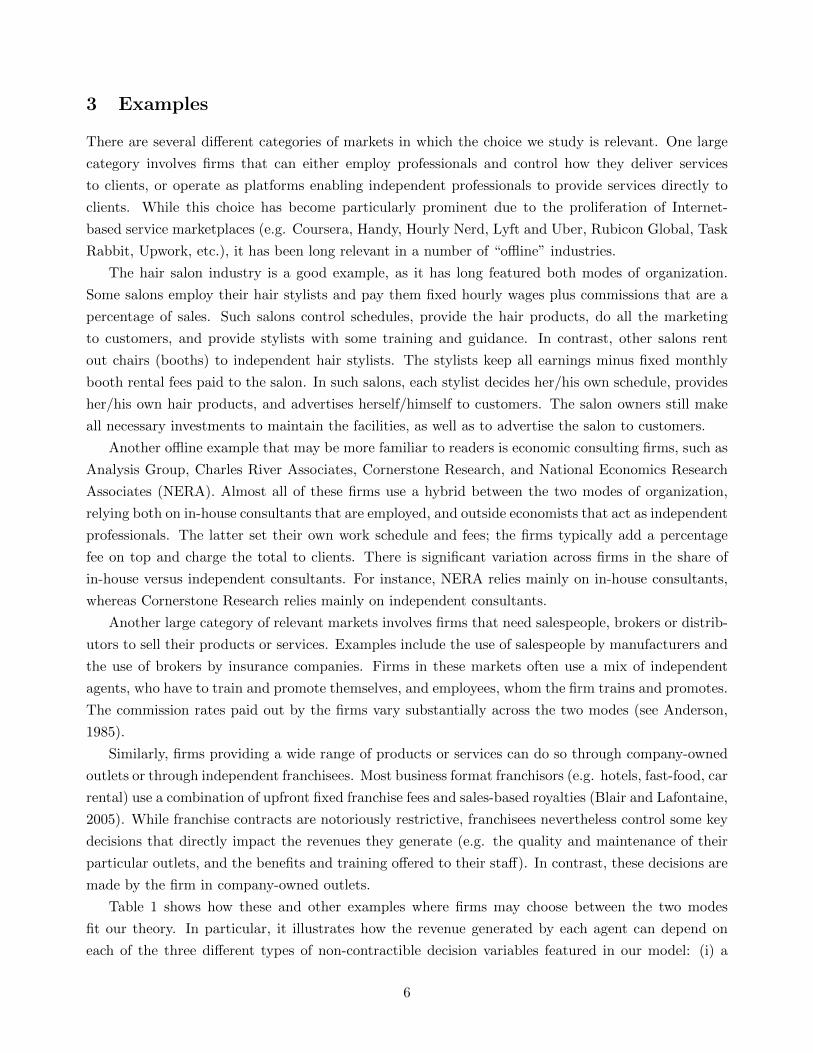
3 Examples

There are several different categories of markets in which the choice we study is relevant. One large

category involves firms that can either employ professionals and control how they deliver services

to clients, or operate as platforms enabling independent professionals to provide services directly to

clients. While this choice has become particularly prominent due to the proliferation of Internet-

based service marketplaces (e.g. Coursera, Handy, Hourly Nerd, Lyft and Uber, Rubicon Global, Task

Rabbit, Upwork, etc.), it has been long relevant in a number of “offline” industries.

The hair salon industry is a good example, as it has long featured both modes of organization.

Some salons employ their hair stylists and pay them fixed hourly wages plus commissions that are a

percentage of sales. Such salons control schedules, provide the hair products, do all the marketing

to customers, and provide stylists with some training and guidance. In contrast, other salons rent

out chairs (booths) to independent hair stylists. The stylists keep all earnings minus fixed monthly

booth rental fees paid to the salon. In such salons, each stylist decides her/his own schedule, provides

her/his own hair products, and advertises herself/himself to customers. The salon owners still make

all necessary investments to maintain the facilities, as well as to advertise the salon to customers.

Another offline example that may be more familiar to readers is economic consulting firms, such as

Analysis Group, Charles River Associates, Cornerstone Research, and National Economics Research

Associates (NERA). Almost all of these firms use a hybrid between the two modes of organization,

relying both on in-house consultants that are employed, and outside economists that act as independent

professionals. The latter set their own work schedule and fees; the firms typically add a percentage

fee on top and charge the total to clients. There is significant variation across firms in the share of

in-house versus independent consultants. For instance, NERA relies mainly on in-house consultants,

whereas Cornerstone Research relies mainly on independent consultants.

Another large category of relevant markets involves firms that need salespeople, brokers or distrib-

utors to sell their products or services. Examples include the use of salespeople by manufacturers and

the use of brokers by insurance companies. Firms in these markets often use a mix of independent

agents, who have to train and promote themselves, and employees, whom the firm trains and promotes.

The commission rates paid out by the firms vary substantially across the two modes (see Anderson,

1985).

Similarly, firms providing a wide range of products or services can do so through company-owned

outlets or through independent franchisees. Most business format franchisors (e.g. hotels, fast-food, car

rental) use a combination of upfront fixed franchise fees and sales-based royalties (Blair and Lafontaine,

2005). While franchise contracts are notoriously restrictive, franchisees nevertheless control some key

decisions that directly impact the revenues they generate (e.g. the quality and maintenance of their

particular outlets, and the benefits and training offered to their staff). In contrast, these decisions are

made by the firm in company-owned outlets.

Table 1 shows how these and other examples where firms may choose between the two modes

fit our theory. In particular, it illustrates how the revenue generated by each agent can depend on

each of the three different types of non-contractible decision variables featured in our model: (i) a

6

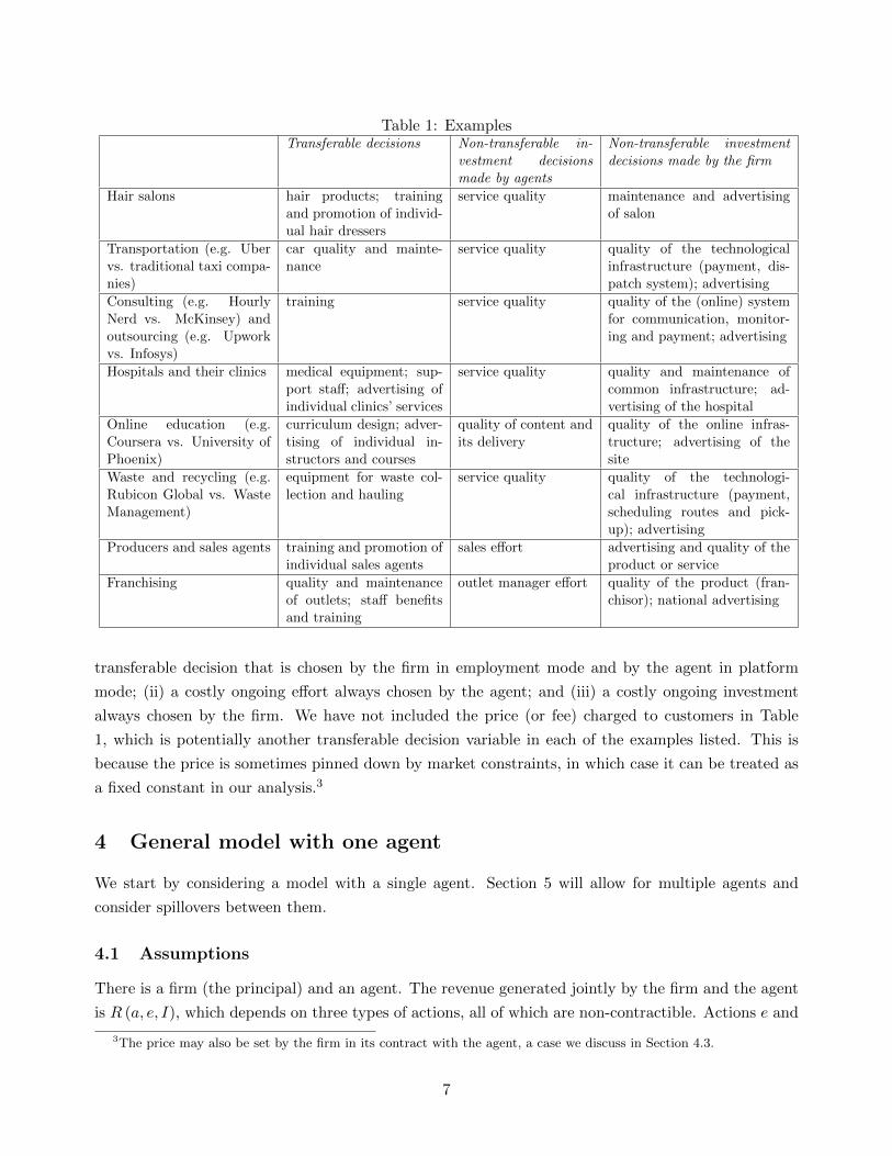
Table 1: ExamplesTransferable decisions Non-transferable in-

vestment decisionsmade by agents

Non-transferable investmentdecisions made by the firm

Hair salons hair products; trainingand promotion of individ-ual hair dressers

service quality maintenance and advertisingof salon

Transportation (e.g. Ubervs. traditional taxi compa-nies)

car quality and mainte-nance

service quality quality of the technologicalinfrastructure (payment, dis-patch system); advertising

Consulting (e.g. HourlyNerd vs. McKinsey) andoutsourcing (e.g. Upworkvs. Infosys)

training service quality quality of the (online) systemfor communication, monitor-ing and payment; advertising

Hospitals and their clinics medical equipment; sup-port staff; advertising ofindividual clinics’ services

service quality quality and maintenance ofcommon infrastructure; ad-vertising of the hospital

Online education (e.g.Coursera vs. University ofPhoenix)

curriculum design; adver-tising of individual in-structors and courses

quality of content andits delivery

quality of the online infras-tructure; advertising of thesite

Waste and recycling (e.g.Rubicon Global vs. WasteManagement)

equipment for waste col-lection and hauling

service quality quality of the technologi-cal infrastructure (payment,scheduling routes and pick-up); advertising

Producers and sales agents training and promotion ofindividual sales agents

sales effort advertising and quality of theproduct or service

Franchising quality and maintenanceof outlets; staff benefitsand training

outlet manager effort quality of the product (fran-chisor); national advertising

transferable decision that is chosen by the firm in employment mode and by the agent in platform

mode; (ii) a costly ongoing effort always chosen by the agent; and (iii) a costly ongoing investment

always chosen by the firm. We have not included the price (or fee) charged to customers in Table

1, which is potentially another transferable decision variable in each of the examples listed. This is

because the price is sometimes pinned down by market constraints, in which case it can be treated as

a fixed constant in our analysis.3

4 General model with one agent

We start by considering a model with a single agent. Section 5 will allow for multiple agents and

consider spillovers between them.

4.1 Assumptions

There is a firm (the principal) and an agent. The revenue generated jointly by the firm and the agent

is R (a, e, I), which depends on three types of actions, all of which are non-contractible. Actions e and

3The price may also be set by the firm in its contract with the agent, a case we discuss in Section 4.3.

7

I are non-transferable: the agent always chooses e ∈ R+ at cost ce (e) and the firm always chooses

I ∈ R+ at cost cI (I). This means there is two-sided moral hazard. To fix ideas, one can think of e

as the effort made by the agent in the provision of its service and of I as capturing the firm’s ongoing

investments (advertising, infrastructure etc.). Action a is transferable, i.e. it can be chosen either by

the firm or by the agent, depending on the mode in which the firm chooses to operate. The party that

chooses a ∈ R+ incurs cost ca (a). Our analysis encompasses two possibilities:

• Costly actions which always increase revenues, i.e. ca (a) > 0 for a > 0 and R increasing in a.

Examples include investments in equipment, training or promotion of agents (see Table 1).

• Costless actions (ca = 0), such that R is single-peaked in a. Price is the most natural example,

but such actions also include “horizontal choices” (see Hagiu and Wright 2015a), such as the

allocation of a fixed promotional capacity between emphasizing the agent’s previous education

and work experience versus her/his performance on recent projects through the firm.

We assume throughout the paper that the only variable that can be contracted on is the realized

revenue R(a, e, I). In other words, any contract offered by the firm to the agent can only depend on

R(a, e, I), but not on any of the underlying variables (a, e, I).

We make the following technical assumptions4:

(a1) All functions are twice continuously differentiable in all arguments.

(a2) The cost functions ce and cI are increasing and strictly convex in their arguments. If ca 6= 0,

then ca is also increasing and strictly convex. Furthermore,

ca (0) = caa (0) = ce (0) = cee (0) = cI (0) = cII (0) = 0.

(a3) The revenue function R is non-negative for all (a, e, I), strictly increasing and weakly concave

in (e, I). If a is costless (i.e. if ca = 0), then R is concave and single-peaked in a for all (e, I). If a is

costly (i.e. if ca 6= 0), then R is strictly increasing and weakly concave in a.

(a4) lime→∞ (Re (a, e, I)− cee(e) < 0) for all (a, I) and limI→∞(RI (a, e, I)− cII(I) < 0

)for all

(a, e). If ca = 0, then for all (e, I) there exists a (e, I) such that R (a, e, I) = 0 for all a ≥ a (e, I). If

ca 6= 0, then lima→∞ (Ra (a, e, I)− caa(a)) < 0 for all (e, I).

(a5) For all t ∈ [0, 1], each of the following two systems of three equations in (a, e, I) admits a

solution: tRa (a, e, I) = caa (a)

(1− t)Re (a, e, I) = cee (e)

tRI (a, e, I) = cII (I)

and (1− t)Ra (a, e, I) = caa (a)

(1− t)Re (a, e, I) = cee (e)

tRI (a, e, I) = cII (I) .

4Subscripts indicate derivatives throughout the paper. Thus, caa indicates the derivative of ca with respect to a, andRa indicates the partial derivative of R with respect to a.

8

These assumptions are standard and are made to ensure that the optimization problems considered

below are well-behaved. Assumption (a4) ensures there is always a finite solution to the optimization

problems we consider. The first set of equations in (a5) are the first-order conditions corresponding

to the employment mode, while the second set of equations in (a5) are the first-order conditions

corresponding to the platform mode.5 If R (a, e, I) is additively separable in its three arguments then

(a5) is implied by (a1)-(a4) and the solution to each of the two sets of equations is unique for all

t ∈ [0, 1].

The firm can choose to operate in one of two modes: E-mode (employment) and P -mode (plat-

form). In both modes, the firm offers the agent a contract consisting of a fixed fee T and a variable fee

tR (a, e, I), where t ∈ [0, 1]. This means the net payment from the agent to the firm is T + tR(a, e, I),

and the agent is left with (1 − t)R(a, e, I) − T . In the next subsection, we show that the restriction

to such linear contracts is without loss of generality. The difference between the two modes is that in

E-mode, the firm controls the transferable action a, whereas in P -mode a is chosen by the agent. This

generally implies different levels of R(a, e, I) across the two modes, and different optimal contracts

(t, T ). Thus, it is possible for T to be negative under E-mode (i.e. the agent receives a fixed wage) and

positive under P -mode (i.e. the agent pays a fixed fee). Nevertheless, if the agent’s outside option is

high enough, then the agent will receive a net payment in both modes. Note also that in our model it

is immaterial whether the firm or the agent collects revenues R (a, e, I) and pays the other party their

share. If in E-mode the firm collects revenues and pays (1− t)R(a, e, I) to the agent, then this can be

interpreted as a bonus in an employment relationship. We assume the firm holds all the bargaining

power. This implies it will set T in both modes so that the agent is indifferent between participation

and her outside option, which for convenience we normalize to zero throughout.

The game we study has the following timing. In stage 0, the firm chooses whether to operate

in E-mode or P -mode. In stage 1, the firm sets (t, T ) and the agent decides whether to accept and

pay the fixed fee T . In stage 2, there are two possibilities depending on the firm’s choice in stage 0.

In E-mode, the firm chooses I and a, and the agent simultaneously chooses e. In P -mode, the firm

chooses I and the agent simultaneously chooses e and a. Finally, in stage 3, revenues R (a, e, I) are

realized; the firm receives tR(a, e, I) and the agent receives (1− t)R(a, e, I).

4.2 General results

We first establish that, given our complete information set-up, the restriction to linear contracts in

both modes is without loss of generality (the proof is in the appendix).

Proposition 1 In both modes, the firm can achieve the best possible outcome with a linear contract.

5A simple sufficient condition for (a5) to hold is that there exist(a, e, I

)such that R (a, e, I)−ca (a)−ce (e)−cI (I) < 0

whenever a > a, e > e or I > I. Indeed, this condition ensures that the relevant space in (a, e, I) is compact, so we canapply the Kakutani fixed point theorem for existence of the solutions to the two systems of equations.

9

This proposition implies that the firm’s profits in E-mode can be written as6

ΠE∗ = maxt,a,e,I

{R (a, e, I)− ca (a)− ce (e)− cI (I)

}(1)

s.t.tRa (a, e, I) = caa (a)

(1− t)Re (a, e, I) = cee (e)

tRI (a, e, I) = cII (I) .

(2)

Similarly, the firm’s P -mode profits are

ΠP∗ = maxt,a,e,I

{R (a, e, I)− ca (a)− ce (e)− cI (I)

}(3)

s.t.(1− t)Ra (a, e, I) = caa (a)

(1− t)Re (a, e, I) = cee (e)

tRI (a, e, I) = cII (I) .

(4)

Assumption (a5) ensures the existence of a solution (a, e, I) to (2) and to (4) for any t ∈ [0, 1]. If

there are multiple solutions for a given t, then the way we have written the optimization programs

implicitly assumes that the firm can choose a stage 2 Nash equilibrium that maximizes its profits.

In general, the respective profits yielded by both modes are lower than the first-best profit level

maxa,e,I

{R (a, e, I)− ca (a)− ce (e)− cI (I)

}.

The reason is that the payoff R (a, e, I) needs to be divided between the firm and the agent in order

to incentivize each of them to choose their respective actions. This inefficiency is the moral hazard in

teams identified by Holmstrom (1982), where a team here consists of the agent and the firm. To reach

the efficient solution, Holmstrom (1982) shows that one needs to break the budget constraint, i.e.

credibly commit to “throw away” revenue in case a target specified ex-ante is not reached. This type

of solution is unrealistic in the contexts we have in mind. Furthermore, our focus is not on offering

general solutions to this class of problems, but rather to analyze the tradeoffs between the two modes

of organization, both of which are unable to reach the first-best.

Comparison of programs (1) and (3) makes it clear that the difference between the two modes

comes from the choice of the non-transferable action a. The tradeoff between the E-mode and the

P -mode boils down to whether it is better to align the choice of a with the firm’s choice of investment

I (E-mode) or with the agent’s choice of effort e (P -mode).

Proposition 2 Compare the firm’s profits under the two modes.

(a) If the transferable action a is contractible or costless (i.e. ca = 0), then the two modes are equivalent

and lead to the same firm profits (ΠE∗ = ΠP∗).

6At the optimum, the fixed fee T of the linear contract is always set such that the participation constraint of theagent is binding, i.e. (1 − t)R (a, e, I) − T − ce (e) = 0.

10

(b) Suppose the transferable action a is non-contractible and costly. If the non-transferable action e

is contractible or if it has no impact on revenue (Re = 0), then ΠE∗ > ΠP∗. If the non-transferable

action I is contractible or if it has no impact on revenue (RI = 0), then ΠP∗ > ΠE∗.

Proof. For (a), if a is contractible, then the constraint in a disappears in both modes, so the programs

(1) and (3) become identical. If ca = 0, then the constraint in a is the same in both modes and is

defined by Ra(a, e, I) = 0, so the two modes are equivalent once again.

For (b), if the agent’s effort has no impact on revenues (Re = 0) then the agent sets e = 0 in both

modes. In E-mode it is then optimal for the firm to retain the entire revenue (t = 1), so profits are

ΠE∗ = maxa,I

{R (a, 0, I)− ca (a)− cI (I)

}.

This is clearly higher than profits under P -mode:

ΠP∗ = maxt,a,I

{R (a, 0, I)− ca (a)− cI (I)

}s.t.{

(1− t)Ra (a, 0, I) = caa (a)

tRI (a, 0, I)− cII (I) .

If the agent’s effort e is contractible, then in E-mode the firm optimally sets t = 1 and profits are

ΠE∗ = maxa,e,I

{R (a, e, I)− ca (a)− ce (e)− cI (I)

}.

This is the first-best level of profits, which strictly dominate the profits that can be achieved in P -mode.

By a symmetric argument, we obtain the result for the case when the firm’s investment has no

impact on revenues (RI = 0) or I is contractible.

Thus, for there to exist a meaningful tradeoff between the two modes with a single agent, (i) all

three actions must be non-contractible and have a strictly positive impact on revenues R, and (ii)

the non-transferable action a must carry a strictly increasing cost ca (a). Part (a) of the proposition

implies that if the transferable action a is price, then, even if it cannot be contracted on, the two modes

are equivalent. As we will see in section 5.4, this no longer holds when there are multiple agents and

there are spillovers from the choice of price corresponding to one agent on the revenues generated by

other agents.

In the general case of interest, when all three actions are non-contractible, have a positive impact

on revenues and carry strictly increasing costs, the two modes distort the choice of a, but they do

so in different ways, leading to different profits. Heuristically, if the firm’s moral hazard (I) is more

important (in the sense that it has a larger impact on R), then the optimal t is higher in both modes,

but then the E-mode induces relatively less distortion in a and is therefore more likely to be preferred.

Conversely, if the agent’s moral hazard (e) is more important, then the optimal t is lower in both

modes, so the P -mode induces less distortion in a and is therefore more likely to be preferred. We

11

confirm this intuition with a linear example below.

Before turning to the linear example, we derive a useful result for the case in which R (a, e, I)

is supermodular in its arguments, i.e. so the actions a, e and I are (weak) strategic complements.

Denote by tE∗ and tP∗ the respective optimal variable fees charged by the firm in the two modes, i.e.

the respective solutions in t that emerge from programs (1) and (3). In the appendix, we prove the

following proposition.

Proposition 3 Suppose R (a, e, I) is supermodular in its arguments. Then, tE∗ < 1/2 implies ΠP∗ >

ΠE∗ and tP∗ > 1/2 implies ΠP∗ < ΠE∗.

The key driving force behind this result is that reducing the distortions in the firm’s and the

agent’s second stage objective functions relative to the firm’s first-stage objective function raises the

firm’s profit. For example, if tE∗ < 1/2, then the distortions can be reduced by shifting control over

the transferable action from the firm to the agent. Indeed, this changes the first-order condition

determining a in the second stage from

tE∗Ra (a, e, I) = caa (a)

to (1− tE∗

)Ra (a, e, I) = caa (a) .

The other two first-order conditions stay unchanged. Given that 1 − tE∗ > tE∗ and that the three

actions are strategic complements, this change results in higher second-stage equilibrium levels of

(a, e, E). This in turn means the outcome is closer to the first-best and therefore equilibrium profits

are higher.

Proposition 3 implies that when the three non-contractible actions are (weak) strategic comple-

ments, the firm would never find it optimal to function in E-mode and pay bonuses above 50% or

function in P -mode and charge variable fees above 50%. This can be re-stated in a more empirically

useful way. To do so, define

t∗ ≡

{tE∗ if ΠE∗ ≥ ΠP∗

tP∗ if ΠE∗ < ΠP∗,

which is the optimal variable fee charged by the firm in the optimal mode. The following corollary is

a logical reformulation of Proposition 3.

Corollary 1 Suppose R (a, e, I) is supermodular in its arguments. Then t∗ ≤ 1/2 if and only if the

P -mode is (weakly) optimal and t∗ ≥ 1/2 if and only if the E-mode is (weakly) optimal.

Thus, according to this prediction of our model, the agent obtains more than 50% of revenues if

and only if the firm is functioning in P -mode. This prediction is supported by the hair salon example.

Traditional hair salons that employ their hair stylists offer bonuses ranging from 35% to 60% of sales,

12

whereas salons that rent out chairs usually charge only a fixed rental fee, letting stylists keep 100% of

sales.7

4.3 Linear example

To illustrate the tradeoff between the E-mode and P -mode in the case of a single agent, assume the

revenue function is linear (and so supermodular) in its arguments:

R (a, e, I) = θa+ γe+ δI, (5)

where θ, γ and δ are all positive constants. The fixed costs are assumed to be

ca (a) =1

2a2, ce (e) =

1

2e2 and cI (I) =

1

2I2. (6)

Thus, γ can be interpreted as the importance of the agent’s moral hazard, whereas δ represents the

importance of the firm’s moral hazard.

Relegating calculations to an online appendix available from the authors’ websites, we obtain

tE∗ =θ2 + δ2

θ2 + γ2 + δ2

tP∗ =δ2

θ2 + γ2 + δ2,

and the following proposition.

Proposition 4 The firm prefers the P -mode to the E-mode if and only if γ > δ.

In other words, the firm prefers the P -mode if the agent’s moral hazard is more important than the

firm’s moral hazard. In particular, in this example the tradeoff does not depend on θ, the impact of the

transferable action on revenues. The reason is that in both modes the share of revenues retained by the

party that chooses the transferable action (tE∗ in E-mode and(1− tP∗

)in P -mode) is increasing in

θ. Since tE∗ and(1− tP∗

)increase at the same rate in this particular example (due to the symmetry

of E-mode and P -mode profits in δ2 and γ2), the resulting tradeoff does not depend on θ.

Note also that tE∗ > tP∗ for all positive (θ, γ, δ). This confirms the common intuition according to

which independent contractors working through platforms should claim a larger share of the revenues

that they directly generate (i.e. a larger commission) than employees working for firms. This is because

in P -mode, sharing revenues with the firm leads to a higher distortion of the transferable variable and

lower profit; by contrast, in E-mode, the more revenue the firm keeps, the lower the distortion of the

transferable variable and the higher the profit. We will see in Section 5.3 that this is no longer always

true with N > 1 agents and spillovers.

7See “Hair & Nail Salons in the US,” IBIS World Industry Report 81211, February 2015.

13

Finally, note that up to this point, we have implicitly assumed the price is fixed, so is held the same

across the two modes, and that there are no production costs. These are not critical assumptions. In

the online appendix, we show that Proposition 4 remains unchanged even if the firm chooses price

along with the fees (t, T ) in its contract, and there are production costs. In other words, the trade-off

between the two modes remains the same, even though the profit maximizing price will differ across

the two modes (it is higher for the mode generating higher profits).

5 General model with multiple agents and spillovers

In this section, we extend the model from Section 4 to N > 1 identical agents and introduce the

possibility that the transferable action ai can also impact the revenue generated by each of the other

agents j 6= i (i.e. that there are spillovers).

5.1 Assumptions

To keep the analysis as streamlined as possible, we assume that revenue is large enough relative to

costs such that it is optimal for the firm to induce all N agents to join in both modes. Then the

revenue attributable to each agent i who joins the firm (in P -mode or E-mode) when all N agents

join is R (ai, si, ei, I), where

si ≡ σ (a−i)

and σ is a symmetric function of the transferable actions chosen by the agents (or for the agents) that

join other than i, with values in R+. In the specific examples used below, σ will be the average of

these other actions, i.e.

σ (a−i) =

∑j 6=i aj

N − 1.

For convenience, we denote by−→a n ≡ (a, ..., a)︸ ︷︷ ︸

n

the vector of n coordinates all equal to a, and by σa (a) the partial derivative of σ (a−i) taken with

respect to any coordinate j 6= i and evaluated at −→a N−1 (by symmetry, all these partial derivatives

are equal). As before, ei is the non-transferable effort chosen by agent i and I is the non-transferable

investment chosen by the firm. Note that the firm chooses a single I that impacts the revenues

attributable to all N agents. Also, R (ai, si, ei, I) does not depend on the choices of non-transferable

actions ej for other agents j 6= i. As we discuss below, introducing this possibility would not add

anything meaningful to the tradeoff between the two modes that we focus on.

The costs of the transferable and non-transferable actions are the same as before and the same

across agents: ca (ai), ce (ei) and cI (I). Finally, the firm is neither allowed to price discriminate across

agents, nor offer an agent a contract contingent on revenues generated by other agents. This means

the firm is restricted to offering the same contract Φ (R) to all agents.

14

The technical assumptions (a1)-(a2) from section 4 remain as before. Assumptions (a3)-(a5) are

adapted as follows:

(a3’) The revenue function R (a, s, e, I) is non-negative for all (a, s, e, I), strictly increasing and

weakly concave in (e, I). If ca = 0, then R (a, s, e, I) is concave and single-peaked in a for all (s, e, I)

and∑N

i=1R (ai, σ (a−i) , ei, I) is concave and single-peaked in all ai for all (ei, I) and i ∈ {1, .., N}. If

ca 6= 0, then R (a, s, e, I) is strictly increasing and weakly concave in a and∑N

i=1R (ai, σ (a−i) , ei, I)

is strictly increasing and weakly concave in all ai, i ∈ {1, .., N}.(a4’) lime→∞ (Re (a, s, e, I)− cee (e)) < 0 for all (a, s, I) and limI→∞

(RI (a, s, e, I)− cII (I)

)< 0

for all (a, s, e). If ca = 0, then for all (s, e, I) there exists a (s, e, I) such that R (a, s, e, I) = 0 for all

a ≥ a (s, e, I). If ca 6= 0, then lima→∞ (Ra (a, s, e, I)− caa (a)) < 0 for all (s, e, I).

(a5’) For all t ∈ [0, 1], each of the following two systems of three equations in (a, e, I) admits a

solution: t (Ra (a, σ (−→a N−1) , e, I) + (N − 1)σa (a)Rs (a, σ (−→a N−1) , e, I)) = caa (a)

(1− t)Re (a, σ (−→a N−1) , e, I) = cee (e)

tNRI (a, σ (−→a N−1) , e, I) = cII (I)

and (1− t)Ra (a, σ (−→a N−1) , e, I) = caa (a)

(1− t)Re (a, σ (−→a N−1) , e, I) = cee (e)

tNRI (a, σ (−→a N−1) , e, I) = cII (I) .

(a6’) The optimization problem solved by the firm admits a well-defined solution which is symmetric

in all N agents in both modes.

The main addition to (a3) is to ensure that the spillover is not so large that it overcomes the “main”

effect of ai. Assumption (a6’) is an additional assumption, which is used to rule out asymmetries in

the optimal solution due to spillovers. The timing is the same as in Section 4.

5.2 General results

We first establish the analogous result to Proposition 1 (the proof is in the appendix).

Proposition 5 If assumptions (a1)-(a2) and (a3’)-(a6’) hold, then in both modes the firm can achieve

the best possible symmetric outcome with a linear contract.

The proposition implies that the firm’s profits in E-mode can be written

ΠE∗ = maxt,a,e,I

{N (R (a, σ (−→a N−1) , e, I)− ca (a)− ce (e))− cI (I)

}(7)

s.t.t (Ra (a, σ (−→a N−1) , e, I) + (N − 1)σa (a)Rs (a, σ (−→a N−1) , e, I)) = caa (a)

(1− t)Re (a, σ (−→a N−1) , e, I) = cee (e)

tNRI (a, σ (−→a N−1) , e, I) = cII (I) .

(8)

15

Similarly, the firm’s profits in P -mode can be written

ΠP∗ = maxt,a,e,I

{N (R (a, σ (−→a N−1) , e, I)− ca (a)− ce (e))− cI (I)

}(9)

s.t.(1− t)Ra (a, σ (−→a N−1) , e, I) = caa (a)

(1− t)Re (a, σ (−→a N−1) , e, I) = cee (e)

tNRI (a, σ (−→a N−1) , e, I) = cII (I) .

(10)

Comparing the two programs above, there are now two differences between the two modes, both

originating in the choice of the non-transferable actions ai. The first difference is the same as in the

case N = 1: the first-order condition in a has a factor t in E-mode and a factor (1− t) in P -mode.

The second difference is new and stems from the presence of spillovers across the N agents: in E-

mode the firm internalizes the spillover when setting ai for i = 1, .., N , whereas the spillovers are left

uninternalized in P -mode when each ai is chosen by individual agent i.

We can now derive the corresponding proposition to Proposition 2.

Proposition 6 Compare the firm’s profits under the two modes.

(a) If the transferable actions ai are contractible, then the two modes are equivalent and lead to the

same firm profits (ΠE∗ = ΠP∗). If the transferable actions are costless and non-contractible (i.e.

ca = 0), then the two modes lead to different profits except when there are no spillovers (Rs = 0).

If in addition the revenue function is additively separable in (a, s), e and I (i.e. if it can be written

R (ai, si, ei, I) = ras (ai, si) + re (ei) + rI (I)), then ΠE∗ > ΠP∗.

(b) Suppose the transferable actions are non-contractible. If the non-transferable actions ei are con-

tractible or if they have no impact on revenue (Re = 0), then ΠE∗ > ΠP∗. If ca = 0 and the

non-transferable action I is contractible or has no impact on revenue (RI = 0), then ΠE∗ > ΠP∗.

Proof. For part (a), if ai is contractible, then the first constraint in (8) and the first constraint in

(10) disappear, so the programs (7) and (9) become identical. If the actions ai carry no cost (ca = 0),

then these first constraints remain distinct in the two modes, unless Rs = 0. Suppose in addition that

R (a, s, e, I) is additively separable. Then, in stage 2, the equilibrium choices of (e, I) as functions of

t are identical in both modes. Denote them by (e (t) , I (t)). The firm’s E-mode profits are then

maxt,a

{Nras (a, σ (−→a N−1)) +N (re (e (t))− ce (e (t))) +NrI (I (t))− cI (I (t))

}s.t. rasa (a, σ (−→a N−1)) + (N − 1)σa (a) rass (a, σ (−→a N−1)) = 0,

which is equal to

maxt,a

{Nras (a, σ (−→a N−1)) +N (re (e (t))− ce (e (t))) +NrI (I (t))− cI (I (t))

}.

16

This is strictly higher than P -mode profits

maxt,a

{Nras (a, σ (−→a N−1)) +N (re (e (t))− ce (e (t))) +NrI (I (t))− cI (I (t))

}s.t. rasa (a, σ (−→a N−1)) = 0.

For part (b), if the agents’ efforts are contractible or if Re = 0, then the firm can achieve the

first-best level of profits in E-mode by setting t = 1, obtaining

ΠE∗ = maxa,e,I

{N (R (a, σ (−→a N−1) , e, I)− ca (a)− ce (e))− cI (I)

}.

In P -mode, we know the resulting profits are strictly lower because the choice of a is not first-best

optimal (it does not account for spillovers).

If ca = 0 and I is contractible or RI = 0, then the firm can once again achieve the first-best level

of profits in E-mode, this time by setting tE arbitrarily close to 0, obtaining

ΠE∗ = maxa,e,I

{N (R (a, σ (−→a N−1) , e, I)− ca (a)− ce (e))− cI (I)

}.

In P -mode it is also optimal to set tP arbitrarily close to 0 but profits are less than first-best because

the choice of a is not first-best optimal (it does not account for spillovers). As a result, ΠE∗ > ΠP∗.

There are two key differences in Proposition 6 relative to Proposition 2. First, due to spillovers,

the case with ca = 0 no longer leads to equivalence. This reflects that in E-mode, spillovers are

internalized, whereas in P -mode they are not. One may think that this always leads to the E-mode to

dominate the P -mode, but this is only true when the revenue function is additively separable in all its

arguments or when I is contractible or when I has no impact on revenue. If instead all three types of

actions are non-contractible and impact revenues and there are interaction effects between a and the

two types of non-transferable investments, then either mode may dominate. In particular, interaction

effects between ai and ei or between ai and I may either exacerbate or dampen the disadvantage of

the P -mode in terms of not internalizing spillovers.

The second difference is that in case (b), contractibility of I or RI = 0 no longer necessarily implies

that the P -mode dominates. The advantage of the P -mode in achieving the constrained first-best level

of ei must still be traded-off against the advantage of the E-mode in internalizing spillovers. At the

extreme, if, in addition, the transferable action is costless, then the E-mode can also achieve the

constrained first-best level of ei, which implies that the E-mode does strictly better.

Note that all the results in Proposition 6 would continue to hold even if we allowed for spillovers of

effort ei across revenues attributable to other agents j 6= i (accompanied by the appropriate changes in

assumptions (a3’)-(a6’)). Indeed, the respective first-order conditions corresponding to e in programs

(7) and (9) would stay the same: the spillover from agents’ efforts remains uninternalized in both E-

mode and P -mode because in both modes agents choose ei’s individually. Thus, the tradeoff between

17

the two modes would not be materially impacted by spillovers generated by the non-contractible,

non-transferable efforts ei. This is why we have abstracted away from such spillovers.

Based on Proposition 6, the two simplest scenarios in which the tradeoff between the two modes

is meaningful are:

1. Costly transferable actions ai and additively separable revenue function R (ai, si, ei, I).

2. Costless transferable actions ai (namely, prices) and non-additively separable revenue function

R (ai, si, ei, I).

The two cases exhibit different mechanisms—we analyze them in the next two subsections through

specific examples. These two cases correspond to realistic scenarios. In many contexts prices are easily

observable and contracted on, which means they do not have an impact on the E-mode versus P -mode

distinction. Alternatively, in other cases parties cannot observe price or quantity separately, so can

only contract on revenue. Then price becomes a relevant transferable and non-contractible variable.

5.3 Linear example with spillovers

This section extends the linear example studied in Section 4.3 to the case of N > 1 agents and

spillovers. Specifically, the revenue generated by agent i is

R (ai, si, ei, I) = θai + x (si − ai) + γei + δI,

where si = σ (a−i) is the average of the transferable actions chosen for j 6= i; i.e.

σ (a−i) =

∑j 6=i aj

N − 1≡ a−i.

We can therefore write directly

R (ai, a−i, ei, I) = θai + x (a−i − ai) + γei + δI.

Costs are assumed to be quadratic as in section 4.3:

cai (a) =1

2a2, cei (e) =

1

2e2 and cI (I) =

1

2I2

Thus, when spillovers are negative (x < 0), revenue R is decreasing in a−i, which means that

in P -mode the transferable actions ai are set too high. Conversely, when spillovers are positive

(x > 0), revenue R is increasing in a−i, so that in P -mode the ai’s are set too low. For example,

if ai represents advertising then negative (respectively, positive) spillovers occur when one agent’s

advertising decreases (respectively, increases) demand realized by other agents.

We assume

x < θ and x (θ − x) < Nδ2, (11)

18

which ensures that (i) assumptions (a1)-(a2) and (a3’)-(a6’) are satisfied for this example, and (ii) the

optimal variable fee is strictly between 0 and 1 in both modes. Note that all x < 0 are permissible

under (11).

We obtain (all calculations are in the online appendix)

tE∗ =θ2 +Nδ2

θ2 + γ2 +Nδ2

tP∗ =Nδ2 − x (θ − x)

(θ − x)2 + γ2 +Nδ2(12)

and the following proposition.8

Proposition 7 The firm prefers the P -mode to the E-mode if and only if

− θ2 −Nδ2 −√θ2 (θ2 + γ2 +Nδ2) + γ4 ≤ xγ

2

θ≤ −θ2 −Nδ2 +

√θ2 (θ2 + γ2 +Nδ2) + γ4. (13)

The right-hand side of (13) is positive if and only if γ2 > Nδ2. The left-hand side is always

negative. Thus, when x = 0 and N = 1, we obtain the result of Proposition 4 that the firm prefers the

P -mode to the E-mode if and only if γ > δ. More generally, if the right-hand side of (13) is positive

so that moral hazard considerations favor the P -mode, then the P -mode is preferred if and only if the

magnitude of spillovers is not too large. (For large spillovers the coordination benefits of the E-mode

dominate.) On the other hand, if the right-hand side is negative so that moral hazard considerations

favor the E-mode, then the P -mode is still preferred if spillovers are sufficiently negative but not

too negative. To understand why, recall that negative spillovers cause the ai’s to be set too high in

P -mode, which partly offsets the primary revenue distortion, i.e. ai’s being set too low because the

party choosing ai does not receive the full marginal return when 0 < t < 1. Thus, when spillovers

are negative, choosing the P -mode (and thereby letting agents choose ai) provides a way for the firm

to commit to achieving a level of ai closer to the first-best. When this effect is moderately strong, it

can offset the advantage of the E-mode if the firm’s moral hazard problem is more important than

that of agents. However, if negative spillovers are too strong, the coordination benefits of the E-mode

dominate once again.

It is straightforward to verify that the entire range of x defined by (13) is permissible by assumptions

(11) for θ sufficiently large. Inspection of (13) reveals that the range of spillover values x for which

the firm prefers the P -mode is skewed towards negative values, consistent with the explanation above.

Positive spillovers cause the ai’s to be set too low in P -mode, which exacerbates the primary revenue

distortion. This makes the P -mode relatively less likely to dominate. When the agents’ moral hazard

8We are no longer able to provide a clear link between the variable revenues obtained by agents and the choice ofmode as in Proposition 3 and Corollary 1. However, in the online appendix we show numerically that knowing whetheragents receive more or less than 50% of variable revenues still allows us to correctly predict the choice of mode most ofthe time.

19

is more important than that of the firm, there still exists a range of positive spillovers for which the

P -mode is preferred, but that range is smaller than the corresponding range of negative spillovers.

The skew towards negative value of x in condition (13) also implies that, if spillovers are moderately

negative, then an increase in their magnitude (i.e. a decrease in x) shifts the trade-off in favor of the P -

mode.9 This result runs counter to the common intuition, according to which spillovers should always

make centralized control (i.e. E-mode in our model) more desirable due to the ability to coordinate

decisions. The reason behind the counter-intuitive result we obtain here is that, as spillovers become

more negative, the commitment benefit of the P -mode in helping increase the level of ai so as to offset

the revenue-sharing distortion becomes stronger. If spillovers are positive or very negative, then the

standard effect is restored.

We now investigate the impact of γ2 and Nδ2 on the tradeoff between P -mode and E-mode, i.e.

on the profit differential ΠP∗ −ΠE∗. From (13), this impact seems difficult to ascertain. Fortunately,

one can use first-order conditions and the envelope theorem, which lead to simple conditions (see the

online appendix for calculations).

Proposition 8 A larger γ shifts the tradeoff in favor of P -mode (i.e.d(ΠP∗−ΠE∗)

d(γ2)> 0) if and only

if tP∗ < tE∗. A larger δ shifts the tradeoff in favor of E-mode (i.e.d(ΠP∗−ΠE∗)

d(Nδ2)< 0) if and only if

tP∗ < tE∗.

In other words, the effects of both types of moral hazard on the tradeoff conform to common

intuition whenever the share of revenues retained by the firm is larger in E-mode. Recall from the

analysis in Section 4.3 that this is always the case in the absence of spillovers. However, with spillovers

this may no longer be the case, so the effects of the two types of moral hazard can be counter-intuitive.

In particular, from (12) we obtain that, with spillovers, tP∗ > tE∗ if and only if

x

θ+

θ

θ − x< −θ

2 +Nδ2

γ2, (14)

i.e. if the spillover x is sufficiently negative (recall that all x < 0 are permissible by assumptions

(11)).10

When the inequality in (14) holds, negative spillovers partially offset the primary revenue-sharing

distortion in P -mode. As a result, a higher t induces less distortion of the transferable actions ai in

P -mode, so the firm can charge a higher t in P -mode, to the point that tP∗> tE

∗. However, when

this occurs, agents retain a lower share of revenues in P -mode than in E-mode, so their choice of non-

transferable effort ei is more distorted in P -mode. Consequently, when agents’ effort (moral hazard)

becomes more important in this parameter region, the E-mode becomes relatively more attractive.

Similarly, when the firm’s investment (moral hazard) becomes more important in the same parameter

9To see this, note that condition (13) can be re-written(x γ

2

θ+ θ2 +Nδ2

)2

≤ θ2(θ2 + γ2 +Nδ2

)+ γ4. Thus, if

−θ2 −Nδ2 < x γ2

θ< 0, then the inequality above is more likely to hold when x decreases.

10It is easily verified that the respective ranges in x defined by (13) and (14) have a non-empty intersection.

20

region, the P -mode becomes relatively more attractive. This counter-intuitive scenario can never occur

in the absence of spillovers in the additively separable case.

5.4 Non-additively separable example (prices)

We now turn to the other case of interest identified in Section 5.2—the transferable action is the price

that is either set by agent i or the firm, and therefore does not carry any costs. Furthermore, in this

case the revenue function is not additively separable, although the underlying demand function is.

Specifically, the revenue generated by agent i is now

R(pi, p−i, ei, I

)= pi

(d+ θpi + x

(p−i − pi

)+ γei + δI

), (15)

where d > 0 is the demand intercept and p−i is the average of the prices chosen for j 6= i. The costs

of the non-transferable actions remain the same as in Section 4.3.

To ensure (a1’)-(a6’) are satisfied for this example, we assume

θ < 0, γ > 0, δ > 0

−2θ + min {0, 2x} > max{Nδ2, γ2

}. (16)

Note that (16) implies all x > 0 are permissible and x > θ, so demand d+ θpi+x(p−i − pi

)+γei+ δI

is decreasing in pi.

From (15), positive spillovers (x > 0) correspond to the usual case with prices: that is, when pi

increases, this increases the demand faced by other agents. Also note that one could replace pi with

qi (quantities), but then the usual case would be captured by negative spillovers (x < 0).

Define

k ≡ 1

Nδ2+

1

γ2∈[

1

|θ|,+∞

).

We then obtain the following proposition (calculations are in the online appendix).

Proposition 9 The firm prefers the P -mode if and only if11

− 4 (1 + θk)

k (1 + 2θk)< x < 0.

First, note that the proposition identifies a meaningful tradeoff since any x satisfying the last

inequality above also satisfies (16) provided θ is sufficiently negative, as do all positive x.

Second, the E-mode is always preferred if spillovers are positive or if spillovers are very negative.

The logic is different here relative to the case with costly transferable actions. Given that the trans-

ferable action here (price) does not carry any costs, there is no distortion of price in either mode due

to revenue-sharing between the firm and each agent. As a result, the variable fee t can be used in both

11Recall θk < −1 so − 4(1+θk)k(1+2θk)

< 0.

21

modes to balance the two-sided moral hazard problem (ei versus I) equally well.12 Furthermore, due

to the strategic complementarity between pi and (ei, I), the choice of pi can either offset or compound

the two moral hazard problems.

The E-mode has an advantage in internalizing spillovers across the agents’ services. This explains

why there is a larger region over which the E-mode dominates. But the fact that agents do not

internalize spillovers in P -mode can work in favor of the P -mode when spillovers are negative (x < 0).

Namely, when x < 0, the P -mode leads to excessively high choices of pi, which can help offset the

two-sided moral hazard problem. This is because a higher pi leads to higher ei and I due to strategic

complementarity, which partially corrects the problem of ei and I being too low that arises from

revenue-sharing. In contrast, when x > 0, the P -mode leads to pi being set too low, which compounds

the two-sided moral hazard problem. As a result, the E-mode always dominates in that case.

Third, the parameters measuring the strength of the two moral hazard problems, Nδ2 and γ2, have

the same effect on the tradeoff between the two modes (through k). This surprising result stands in

contrast to the additively separable case where they work in opposing directions. The explanation is

as follows. Again, since the transferable action (price) is not distorted by the variable fee t in either

mode, both modes do just as well in terms of balancing the two-sided moral hazard problem. As

noted above, when spillovers are negative, raising prices reduces the moral hazard problems due to

the strategic complementarity between prices and investments, and this works equally well for both

ei and I. Thus, the extent to which the P -mode is preferred over the E-mode when moral hazard

problems become more important does not depend on the source of the moral hazard, but only on its

magnitude.

Finally, it is easily verified that − 4(1+θk)k(1+2θk) is decreasing for k ∈

[1|θ| ,

1|θ| +

√2

2|θ|

]and increasing for

k ≥ 1|θ| +

√2

2|θ| . Thus, assuming negative spillovers, when γ2 and Nδ2 are small (i.e. k large), the

range of x over which the P -mode is preferred increases as γ2 and Nδ2 increase (i.e. k decreases); and

vice versa when γ2 and Nδ2 are large (k small). In other words, when the two-sided moral hazard

problem is of small importance, the effectiveness of the P -mode in compensating for moral hazard

with excessive prices increases as moral hazard becomes more important, so the tradeoff shifts in favor

of the P -mode. And vice versa when two-sided moral hazard is already very important.

6 Extensions

This section explores several extensions to our model: allowing for private benefits, changing the

timing of the infrastructure investment I; cost asymmetries between the firm and the agent(s); and

allowing the firm to choose a hybrid mode that lies between the pure E-mode and pure P -mode.

12For this reason, there is no underlying tendency to have a high t under E-mode and a low t under P -mode. Thus,knowing whether agents receive more or less than 50% of variable revenues does not in general help predict the choice ofmode when the transferable action is costless.

22

6.1 Private benefits

Consider the benchmark model with one agent from Section 4. The transferable action a can drive

an additional wedge between the two modes when one or both parties derive private benefits from the

choice of a. Examples of private benefits include the enhancement of individual agents’ reputation

and outside opportunities by the marketing of their services (e.g. hair dressers, consultants, sales

representatives) and the improved reputation of the firm by the choice of better equipment (e.g. hair

salons, hospitals and clinics, taxi companies).

Formally, suppose that a influences some non-contractible outside payoffs, Y (a) for the firm and

y (a) for the agent, where the functions Y and y are non-negative, twice-continuously differentiable

and increasing. It is easily seen that the proof of Proposition 1 continues to apply, so linear contracts

remain optimal in both modes.13

Private benefits change the programs (1) and (3) that determine E-mode and P -mode profits in

two ways. First, since the agent’s private benefit affects its willingness to participate, the function

maximized by the firm in both modes is now

R (a, e, I) + Y (a) + y (a)− ca (a)− ce (e)− cI (I) .

Second, the first-order condition in a for the E-mode is now14

tRa (a, e, I) + Ya (a) = caa (a) , (17)

while the new first-order condition in a for the P -mode is

(1− t)Ra (a, e, I) + ya (a) = caa (a) . (18)

Comparing the new first-order conditions (17) and (18) with the ones in the programs (2) and (4),

it is clear that Proposition 2 no longer holds. In particular:

• even if a is costless, as long as the private benefit functions y and Y are different, the resulting

profits in E-mode and P -mode are different.

• even if e (respectively, I) is contractible or does not impact revenues, the P -mode (respectively,

E-mode) might still dominate if y (respectively, Y ) is sufficiently large.

Heuristically, holding everything else constant, if the firm’s private benefit Y is more (respectively,

less) important than the agent’s private benefit y, then the E-mode is more (respectively, less) likely

to be preferred to the P -mode.

As in Section 4.3, we can reach more precise results by imposing supermodularity on R. In the

online appendix we extend Proposition 3 and Corollary 1 to the case with linear private benefits, i.e.

13We just need to assume R (a, e, I) + Y (a) + y (a) is single-peaked in a if ca = 0 or increasing in a if ca > 0, andadjust assumptions (a1), (a4) and (a5) accordingly.

14The reason we focus on private benefits influenced by a only is that any private benefit influenced by e or I wouldnot create any difference between the sets of first-order conditions (2) and (4) corresponding to the two modes.

23

Y (a) = Y a and y (a) = ya. This provides a way to continue to predict which mode a firm is operating

in based on the observed share of variable revenues retained by the agent. We also obtain a precise

comparison of the two modes by resorting to the linear additively separable example of Section 4.3,

to which we add linear private benefits Y (a) = Y a and y (a) = ya.15 Extending Proposition 4 to this

case, we obtain that the firm prefers the P -mode to the E-mode if and only if((θ + y)2 − Y 2

)γ2 >

((θ + Y )2 − y2

)δ2.

Thus, the tradeoff is shifted in favor of the P -mode when the agent’s moral hazard and private benefit

become more important and in favor of the E-mode when the firm’s moral hazard and private benefit

become more important. Note that y = Y implies ΠP∗ > ΠE∗ if and only if γ > δ, i.e. the baseline

trade-off is restored when the private benefits of the two parties are equally important. Furthermore,

γ = δ implies ΠP∗ > ΠE∗ if and only if y > Y . In other words, if the agent’s and the firm’s moral

hazard are equally important, then the choice of mode only depends on which party’s private benefits

are more important.

6.2 Timing

When I represents a basic infrastructure investment that is fundamental to the firm’s operations, in

some cases this investment is made prior to the choice of business model (E-mode versus P -mode),

rather than afterwards. This reflects that it may be easier for a firm to change its business model than

its basic infrastructure. In this case, the model becomes very similar to that in Hagiu and Wright

(2015b), but without private information.

The net result of this change in timing is to shift the firm’s business model tradeoff in favor of

the P -mode. Indeed, if the firm is able to commit to its choice of I prior to the choice of business

model, then the need to keep a larger share of variable revenues in order to motivate investments in

I disappears. This observation implies that one of the factors that determines the choice of mode is

the extent to which the firm’s investments are determined upfront. Thus, when the firm’s ongoing

investments in infrastructure (or other forms of common investment) increase in importance relative

to its ex-ante investments, the tradeoff shifts in the same way predicted by our analysis above when

the firm’s moral hazard problem becomes more important.

6.3 Cost asymmetries

Throughout the analysis above we have assumed there are no asymmetries between the firm and the

agent(s) in the costs of undertaking the transferable action or in its impact on revenues. In some

real-world examples, such asymmetries are an important factor in determining which control rights

are held by the firm and which are held by agents. For example, the firm may have economies of scale

advantages over individual agents when incurring the cost associated with the transferable action a

15If instead the private benefits are assumed to be proportional to the demand underlying the linear revenue function,they will be irrelevant for the tradeoff between the two modes. See online appendix.

24

(e.g. economies of scale in purchasing equipment) or better information regarding the impact of the

transferable action on revenues due to access to more data (e.g. Uber and Lyft when setting prices

for rides).

Introducing cost asymmetries between the firm and the agent is straightforward in our model with

one agent. We simply assume that the cost of the transferable action a is caE (a) when incurred

by the firm in E-mode and caP (a) when incurred by the agent in P -mode, where the functions caE

and caP have the same properties as previously assumed for the function ca. Proposition 1 continues

to hold for both modes, such that the optimal contracts are linear. It is easily seen that a higher

relative cost advantage for the firm (respectively, the agent) shifts the trade-off in favor of the E-mode

(respectively, P -mode). Such cost asymmetries are not equivalent to the asymmetric private benefits

studied in section 6.1. With cost asymmetries, the total payoff maximized by the firm changes from

one mode to the other, which was not the case with private benefits.

6.4 Hybrid mode across agents

Hybrid modes, with some agents offering their services in E-mode and others in P -mode, are found

quite often in the markets we consider (e.g. consultancies, sales representatives for industrial compa-

nies). In this subsection we show that a strictly hybrid mode can be optimal even without spillovers

(i.e. we assume Rs = 0) and despite the fact that all N agents are identical. This is due to the fact

that I is a common investment across all the agents’ services (e.g. a common infrastructure), and to

the concavity of the profit function with respect to I.

We use the linear example from Section 5.3 with no spillovers (x = 0) and quadratic costs. At first

glance, this seems like the least likely scenario for a hybrid mode to be optimal, because there are no

interaction effects and no asymmetries between firm and agents.

Suppose the firm functions in E-mode with respect to agents i ∈ {1, .., n} and in P -mode with

respect to agents i ∈ {n+ 1, .., N}, where n ≤ N . Thus, the firm offers contract(tE , TE

)to the n

agents that work in E-mode (employees) and contract(tP , TP

)to the N − n agents that work in

P -mode (independent contractors). The n employees each choose a level of effort equal to(1− tE

)γ,

whereas the N −n independent contractors each choose a level of effort equal to(1− tP

)γ and a level

of the transferable activity equal to(1− tP

)θ. For the n employees, the firm chooses a level of the

transferable action equal to tEθ. Finally, the level I(tE , tP

)chosen by the firm is I

(tE , tP

)= tNδ,

where

t ≡ n

NtE +

N − nN

tP

is the “average” transaction fee collected by the firm.

The fixed fees for employees and independent contractors are set to render both indifferent between

25

working for/through the firm and their outside option. Consequently, the total profit of the firm is

ΠH(tE , tP , n

)= n

tE (2− tE) θ2

2+

(1−

(tE)2)

γ2

2

+ (N − n)

(

1−(tP)2)

θ2

2+

(1−

(tP)2)

γ2

2

+t(2− t

)N2δ2

2.

Sincet(2−t)

2 is concave in t, it is easily seen that the optimal choice of n can be interior (i.e. strictly

between 0 and N). The key reason is that the firm can only choose a single I, which affects all agents.

If the firm could choose different Ii’s for each individual agent i, then the optimal solution would be

n = N or n = 0. Since the firm’s profit function is concave with respect to I, the firm does better

with an intermediate value of I (i.e. that arising from a mix of modes) than it would get from having

all agents in one mode or the other.

The optimal number of employees is (see the online appendix for the full derivation)

n∗ =

N if Nδ2 > θ2 + γ2

N

(1− γ2(θ2+γ2−Nδ2)

2Nδ2θ2

)if θ2 + γ2 > Nδ2 > γ2 − θ2γ2

2θ2+γ2

0 if Nδ2 < γ2 − θ2γ2

2θ2+γ2.

Note that n∗ is increasing in Nδ2 (the importance of the firm’s moral hazard) and decreasing in

γ2 (the importance of agents’ moral hazard), consistent with the intuition built in Section 5.3 for the

case x = 0.

6.5 Hybrid modes across actions

Up to here, we have always restricted attention to a single transferable action for concision. In many

real-world examples, however, there are multiple relevant transferable actions (see Table 1 in Section

3). This provides another dimension along which firms can (and oftentimes do) operate in hybrid

modes, with some transferable decisions controlled by agents and others by the firm.

Our model can be extended to encompass this dimension as well. Consider the case with one agent

but multiple transferable actions, aj , with j ∈ {1, ..,M}, so the revenue function is R(a1, .., aM , e, I

).

The fixed cost associated with transferable action aj is caj (aj). The costs associated with non-

transferable actions are ce (e) and cI (I) as before.

The firm optimizes its profits over the contract (t, T ) and the set A ⊂ {1, ..,M} of decisions

over which it keeps control (the agent controls decisions j ∈ {1, ..,M} \A). The following proposi-

tion (proven in the appendix) establishes that the hybrid interior mode can never be optimal when

R(a1, .., aM , e, I

)is supermodular in its arguments.

Proposition 10 If the revenue function R is supermodular in(a1, .., aM , e, I

), then the optimal mode

is either A = ∅ (P -mode) or A = {1, ..,M} (E-mode).

26

The key driving force behind the result in Proposition 10 is that reducing the distortions in the

firm’s and the agent’s second stage objective functions relative to the firm’s first-stage objective func-

tion raises the firm’s profit. If t∗ < 1/2, the distortions can be reduced by giving control over all

transferable actions to agents. If t∗ > 1/2, the distortions can be reduced by giving control over all

transferable actions to the firm. Only in the special case when t∗ = 12 , would any split of control

rights, including a strictly interior split, be optimal. However, the proposition still applies given that

pure modes remain weakly optimal in this case. Given our symmetric set-up with no cost differences

between the firm and the agent in choosing the transferable actions, the proposition supports our focus

throughout the paper on pure modes and suggests that a strictly interior split of control rights can

only be optimal if there are negative interaction effects across the actions (ai, e, I).

Alternatively, allowing for asymmetries here (as in Section 6.3 above) would provide a natural way

of explaining which control rights are held by the firm and which are held by agents. For instance,

Uber and Lyft have a clear advantage in setting prices for rides over their drivers (better information),

wheareas drivers are in a better position to choose their work schedules and the amount of maintenance

their individual cars need. Hair salons may take control over the choice of “uniforms” because they

can obtain lower costs due to scale effects (relative to individual hair stylists), but the marketing of

hair stylists may be more efficiently done by each individual.

7 Conclusion

By substantially reducing the costs of remote monitoring, communication and collaboration, Internet

and mobile technologies have made it possible to build marketplaces and platforms for a rapidly

increasing variety of services, ranging from house cleaning to programming, consulting and legal advice.

As a result, the choice between platform mode and employment mode and the associated tradeoffs

that we have examined in this paper are becoming increasingly relevant in a growing number of sectors

throughout the economy.

At the most fundamental level, we have shown that the tradeoffs arise from balancing two-sided

moral hazard, while at the same time minimizing distortions in the choice of transferable actions due

to revenue-sharing or spillovers. Our modelling approach and some of our key results are reminiscent

of the theory of the firm based on property rights and incentive systems. In particular, in the baseline

model without spillovers, a key prediction is that control rights over transferable actions should be

given to whichever party’s (the firm or the agents) moral hazard problem is more important. However,

we have shown that this prediction can be over-turned when spillovers are introduced, both with costly

and costless transferable actions. In particular, when the transferable action is price (and therefore

there are interaction effects with the non-transferable actions), the tradeoff between the two modes

no longer depends on the source of moral hazard, but only on its magnitude. These insights are novel

and contribute to extending the theory of the firm based on property rights and incentive systems to

new types of organizational choices.

Our analysis is also relevant to current legal and regulatory debates about whether “sharing econ-

27

omy” service marketplaces (e.g. Handy, Lyft, Postmates, Uber) should be forced to treat professionals

that work through them as employees rather than independent contractors.16 All existing legal def-

initions emphasize control rights as the most important factor in determining this issue, which is

consistent with our analysis. On the other hand, the assignment of fixed costs to one party or the

other would seem to matter much less for the distinction. Indeed, a simple observation based on our

model is that any fixed cost that would be borne by the firm in E-mode and by independent contrac-

tors in P -mode (e.g. health insurance, worker tax filings) makes no difference to the tradeoff between

the two modes. Although such a cost is not directly incurred by the firm in P -mode, it nevertheless

has to adjust the fixed fee charged to agents downward relatively to the E-mode, in order to fully

account for the higher cost incurred by agents (assuming the outside option is unchanged). However,

in practice, some of the fixed costs incurred by the firm in E-mode are not pure transfers to workers

(e.g. compliance costs). This drives a fixed cost wedge between the two modes, shifting the tradeoff

in favor of the P -mode, but other considerations in our model continue to hold.

Needless to say, there are other considerations that are relevant to the policy debate regarding

the proper boundary between employees and independent contractors, but are not captured in our

model: the impact of the work being done and the control rights associated with it on agents’ outside

options, the intensity of competition faced by the firms, the efficiency effects of different regulatory

and tax regimes on firms’ choices between the two options. Incorporating some of these aspects into

the analysis provides a promising avenue for future research based on our work in this paper. There

are several other directions in which our work can be extended. One would be to allow the firm to

charge customers a fixed access fee in both modes and study the impact of such a fee on the tradeoff

between the two modes. Such a fee is used by some firms selling some basic hardware or software

to consumers, which is required in order to access the relevant services or products (e.g. video-game

consoles). Another direction would be to study competition among firms that can each choose between

the employment mode and the platform mode, potentially leading to equilibria in which firms compete

with different models. Finally, one could pursue the analysis of hybrid modes along the lines briefly

described in Section 6 by incorporating cost or information asymmetries between the firm and the

agents and determining their effect on the optimal allocation of control rights.

References

[1] Anderson, E. (1985) “The Salesperson as Outside Agent or Employee: A Transaction Cost Anal-

ysis.” Marketing Science, 4(3), 234-54.

[2] Blair, R. D. and F. Lafontaine (2005) The Economics of Franchising, New York, NY: Cambridge

University Press.

[3] Evans, D. S., A. Hagiu and R. Schmalensee (2006) Invisible Engines: How Software Platforms

Drive Innovation and Transform Industries, Cambridge, MA: The MIT Press.

16See for example Justin Fox “Uber and the Not-Quite-Independent Contractor” Bloomberg, June 30, 2015.

28

[4] Gawer A. and M. Cusumano (2002) Platform Leadership: How Intel, Microsoft, and Cisco Drive

Industry Innovation, Boston, MA: Harvard Business School Press.

[5] Gawer, A. and R. Henderson (2007) “Platform Owner Entry and Innovation in Complementary

Markets: Evidence from Intel,” Journal of Economics & Management Strategy, 16(1), 1-34.

[6] Gibbons, R. (2005) “Four Formal(izable) Theories of the Firm?” Journal of Economic Behavior

& Organization, 58, 200–245.

[7] Grossman, S. and O. Hart (1986) “The Costs and Benefits of Ownership: A Theory of Vertical

and Lateral Ownership,” Journal of Political Economy, 94(4), 691–719.

[8] Hagiu, A. and J. Wright (2013) “Do You Really Want to Be an eBay?” Harvard Business Review,

91(3), 102–108.

[9] Hagiu, A. and J. Wright (2015a) “Marketplace or Reseller?” Management Science, 61(1), 184–203.

[10] Hagiu, A. and J. Wright (2015b) “Multi-sided Platforms” International Journal of Industrial

Organization, forthcoming.

[11] Hart, O. and J. Moore (1990) “Property rights and the nature of the firm,” Journal of Political

Economy, 98, 1119–1158.

[12] Holmstrom, B. (1982) “Moral Hazard in Teams,” Bell Journal of Economics, 13(2), 324-340.

[13] Holmstrom, B. and P. Milgrom (1987) “Aggregation and Linearity in the Provision of Intertem-

poral Incentives,” Econometrica, 55(2), 303-328.

[14] Holmstrom, B. and P. Milgrom (1994) “The Firm as an Incentive System,” American Economic

Review, 84(4), 972-991.

[15] Romano, R. E. (1994) “Double Moral Hazard and Resale Price Maintenance,” Rand Journal of

Economics, 25(3), 455–466.

[16] Rysman, M. (2009) “The Economics of Two-Sided Markets,” Journal of Economic Perspectives,

23, 125-143.

[17] Wernerfelt, B. (2002) “Why Should the Boss Own the Assets,” Journal of Economics & Manage-

ment Strategy, 11(3), 473-485.

29

Appendix

Proof of Proposition 1

The optimal contract Φ∗ (R) (i.e. payment to the agent) chosen by the firm in E-mode solves

ΠE∗ = maxΦ(.),a,e,I

{R (a, e, I)− Φ (R (a, e, I))− ca (a)− cI (I)

}s.t.

a = arg maxa′ {R (a′, e, I)− Φ (R (a′, e, I))− ca (a′)}e = arg maxe′ {Φ (R (a, e′, I))− ce (e′)}I = arg maxI′

{R (a, e, I ′)− Φ (R (a, e, I ′))− cI (I ′)

}0 ≤ Φ (R (a, e, I))− ce (e) .

We start by proving the following lemma.

Lemma 1 Φ∗ (R) must be continuous and differentiable at R∗ = R (a∗, e∗, I∗), where R∗ is the revenue

that results from the optimization problem above.

Proof. Suppose Φ∗ is discontinuous at R∗ and limR→R∗− Φ∗ (R) > limR→R∗+ Φ∗ (R). Then

I∗ = arg maxI

{R (a∗, e∗, I)− Φ∗ (R (a∗, e∗, I))− cI (I)

}implies Φ∗ (R∗) = limR→R∗+ Φ∗ (R), because otherwise Φ∗ (R∗) > limR→R∗+ Φ∗ (R), so the firm could

profitably deviate to I∗ + ε, with ε sufficiently small. But then we must have e∗ = 0, since otherwise

e∗ > 0 and the agent could profitably deviate to e∗ − ε with ε sufficiently small. If e∗ = 0, then it

must be that Φ∗ (R∗) = 0 and therefore

(a∗, I∗) = arg maxa,I

{R (a, 0, I)− ca (a)− cI (I)

}. (19)

In this case the firm could switch to the following linear contract:

Φε (R) = εR+ ce (e (ε))− εR (a (ε) , e (ε) , I (ε)) ,

where ε > 0 is sufficiently small and (a (ε) , e (ε) , I (ε)) is a solution toa (ε) = arg maxa {R (a, e (ε) , I (ε))− Φε (R (a, e (ε) , I (ε)))− ca (a)}e (ε) = arg maxe {Φε (R (a (ε) , e, I (ε)))− ce (e)}I (ε) = arg maxI

{R (a (ε) , e (ε) , I)− Φε (R (a (ε) , e (ε) , I))− cI (I)

}.

Denote the firm profits that result from offering contract Φε by

ΠE (ε) ≡ R (a (ε) , e (ε) , I (ε))− ca (a (ε))− ce (e (ε))− cI (I (ε)) .

30

Clearly, (a (0) , e (0) , I (0)) = (a∗, 0, I∗) and ΠE (0) = ΠE∗. We can then use (19), the definition of

e (ε) and assumption (a2) to obtain

ΠEε (0) = (Ra (a∗, 0, I∗)− caa (a∗)) aε(0) + (Re (a∗, 0, I∗)− cee (0)) eε(0)

+(RI (a∗, 0, I∗)− cII (I∗)

)Iε(0)

= Re (a∗, 0, I∗)Re (a∗, 0, I∗)

ceee (0)> 0,

where ceee = d2ce

de2.

Thus, if limR→R∗− Φ∗ (R) > limR→R∗+ Φ∗ (R), then the firm can profitably deviate to Φε (R) for ε

small enough, which contradicts the optimality of Φ∗ (R).

The other possibility is limR→R∗+ Φ∗ (R) > limR→R∗− Φ∗ (R). Then e∗ = arg maxe {Φ∗ (R (a∗, e, I∗))− ce (e)}implies Φ∗ (R∗) = limR→R∗+ Φ∗ (R), because otherwise Φ∗ (R∗) < limR→R∗+ Φ∗ (R), so the agent could

profitably deviate to e∗ + ε, with ε sufficiently small. But then we must have I∗ = 0, otherwise the

firm could profitably deviate to I∗ − ε with ε sufficiently small.

If a is not price, then Ra (a, e, I) > 0 for all (a, e, I) so the same logic implies a∗ = 0. We must

then have

ΠE∗ = R (0, e∗, 0)− ce (e∗) = maxe{R (0, e, 0)− ce (e)} . (20)

This cannot be optimal. Indeed, the firm could switch to the linear contract

Φε (R) = (1− ε)R+ ce (e (ε))− (1− ε)R(a (ε) , e (ε) , I (ε)

),

where ε > 0 is sufficiently small and(a (ε) , e (ε) , I (ε)

)is a solution to

a (ε) = arg maxa

{R(a, e (ε) , I (ε)

)− Φε

(R(a, e (ε) , I (ε)

))− ca (a)

}e (ε) = arg maxe

{Φε

(R(a (ε) , e, I (ε)

))− ce (e)

}I (ε) = arg maxI

{R (a (ε) , e (ε) , I)− Φε (R (a (ε) , e (ε) , I))− cI (I)

}.

Denote the firm profits that result from offering contract Φε by

ΠE (ε) ≡ R(a (ε) , e (ε) , I (ε)

)− ca (a (ε))− ce (e (ε))− cI

(I (ε)

).

Clearly,(a (0) , e (0) , I (0)

)= (0, e∗, 0) and ΠE (0) = ΠE∗. Using (20), the definitions of a (ε) and

I (ε) and assumption (a2), we obtain

ΠEε (0) = Ra (0, e∗, 0) aε (0) + (Re (0, e∗, 0)− cee (e∗)) eε (0)

+RI (0, e∗, 0) Iε (0)

= Ra (0, e∗, 0)Ra (0, e∗, 0)

caaa (0)+RI (0, e∗, 0)

RI (0, e∗, 0)

cIII (0)> 0,

31

where caaa = d2ca

da2and cIII = d2cI

dI2.

Thus, the firm can profitably deviate to Φε (R) for ε small enough, which contradicts the optimality

of Φ∗ (R).

If a is price, then ca = 0 so we must have

ΠE∗ = R (a∗, e∗, 0)− ce (e∗) ≤ maxa,e{R (a, e, 0)− ce (e)} .

Once again, it is straightforward to verify that the firm could profitably deviate to Φε (R) for ε small

enough.

We have thus proven that limR→R∗+ Φ∗ (R) = limR→R∗− Φ∗ (R), so Φ∗ is continuous at R∗.

Suppose now that Φ∗ is non-differentiable at R∗ and limR→R∗+ Φ∗R (R) > limR→R∗− Φ∗R (R). This

implies e∗ = 0, otherwise we must have

0 ≥ lime→e∗+

{Φ∗R (R (a∗, e, I∗))Re (a∗, e, I∗)− cee (e)} > lime→e∗−

{Φ∗R (R (a∗, e, I∗))Re (a∗, e, I∗)− cee (e)} ,

so setting e slightly below e∗ would violate e∗ = arg maxe {Φ (R (a∗, e, I∗))− ce (e)}. If e∗ = 0, then

we must have Φ∗ (R∗) = 0 (recall ce (0) = 0) and therefore

(a∗, I∗) = arg maxa,I

{R (a, 0, I)− ca (a)− cI (I)

}.

But then we can apply the same reasoning as above to conclude that the firm could profitably devaite

to the linear contract Φε (R) for ε small enough.

Suppose instead limR→R∗+ Φ∗R (R) < limR→R∗− Φ∗R (R). This implies I∗ = 0, otherwise we must

have

0 ≤ limI→I∗−

{RI (a∗, e∗, I) (1− Φ∗R (R (a∗, e∗, I)))− cII (I)

}< lim

I→I∗+

{RI (a∗, e∗, I) (1− Φ∗R (R (a∗, e∗, I)))− cII (I)

},

so setting I slightly above I∗ would violate I∗ = arg maxI{R (a∗, e∗, I)− Φ (R (a∗, e∗, I))− cI (I)

}.

If action a is not price, then ca 6= 0 and Ra > 0, so that the exact same reasoning applies to a∗

and leads to a∗ = 0. This would mean that

ΠE∗ = R (0, e∗, 0)− ce (e∗) ≤ maxe{R (0, e, 0)− ce (e)} .

We have already proven above that this cannot be optimal.

If action a is price, then ca = 0 and

ΠE∗ = R (a∗, e∗, 0)− ce (e∗) ≤ maxa,e{R (a, e, 0)− ce (e)} .

In this case, we have proven above that the firm could do strictly better with the linear contract Φε (R)

32

for ε small enough.

We conclude that Φ∗ (.) must be continuous and differentiable at R∗.

The lemma implies that (a∗, e∗, I∗) solveRa (a∗, e∗, I∗) (1− Φ∗R (R∗)) = caa (a∗)

Re (a∗, e∗, I∗) Φ∗R (R∗) = cee (e∗)

RI (a∗, e∗, I∗) (1− Φ∗R (R∗)) = cII (I∗) .

Let then t∗ ≡ 1 − Φ∗R (R∗) and T ∗ ≡ (1− t∗)R∗ − Φ∗ (R∗). Clearly, the linear contract Φ (R) =

(1− t∗)R−T ∗ can generate the same stage 2 equilibrium as the initial contract Φ∗ (R). Furthermore,

both Φ∗ (R) and Φ (R) cause the agent’s participation constraint to bind and therefore result in the

same profits for the firm.

A similar proof applies to the case when the firm chooses the P -mode.

Proof of Proposition 5

Consider first the E-mode. By (a6’) it is optimal for the firm to induce all N agents to join, so the

optimal contract Φ∗ (.) (i.e. payment to each agent) solves

ΠE∗ = maxΦ(.),I,(ai,ei)i=1,..,N

{N∑i=1

[R (ai, σ (a−i) , ei, I)− Φ (R (ai, σ (a−i) , ei, I))− ca (ai)]− cI (I)

}s.t.

(a1, .., aN ) = arg max(a′1,..,a′N)

{∑Ni=1

(R(a′i, σ

(a′−i), ei, I

)− Φ

(R(a′i, σ

(a′−i), ei, I

))− ca (a′i)

)}ei = arg maxe′i {Φ (R (ai, σ (a−i) , e

′i, I))− ce (e′i)} for all i ∈ {1, .., N}

I = arg maxI′{∑N

i=1 [R (ai, σ (a−i) , ei, I′)− Φ (R (ai, σ (a−i) , ei, I

′))]− cI (I ′)}

0 ≤ Φ (R (ai, σ (a−i) , ei, I))− ce (ei) for all i ∈ {1, .., N} .

By assumption (a6’), we know that the solution to this program is symmetric, so we can write

ΠE∗ = maxΦ(.),I,a,e

{N [R (a, σ (−→a N−1) , e, I)− Φ (R (a, σ (−→a N−1) , e, I))− ca (a)]− cI (I)

}(21)

s.t.

a = arg maxa′

{R (a′, σ (−→a N−1) , e, I)− Φ (R (a′, σ (−→a N−1) , e, I))

+ (N − 1) (R (a, σ (a′,−→a N−2) , e, I)− Φ (R (a, σ (a′,−→a N−2) , e, I)))− ca (a′)

}e = arg maxe′ {Φ (R (a, σ (−→a N−1) , e′, I))− ce (e′)}I = arg maxI′

{N [R (a, σ (−→a N−1) , e, I ′)− Φ (R (a, σ (−→a N−1) , e, I ′))]− cI (I ′)

}0 ≤ Φ (R (a, σ (−→a N−1) , e, I))− ce (e) .

Let then (a∗, e∗, I∗) denote the symmetric outcome of this optimization problem. Also define R∗ ≡R(a∗, σ

(−→a∗N−1

), e∗, I∗

).

Lemma 2 Φ∗ (.) is continuous and differentiable at R∗.

33

Proof. Due to symmetry, the proof is almost identical to the one of lemma 1, so we omit it. In

particular, assumption (a5’) ensures that the deviation contracts Φε and Φε yield the desired result,

just like in lemma 1.

The lemma and program (21) imply that (a∗, e∗, I∗) solve(1− Φ∗R (R∗))

(Ra

(a∗, σ

(−→a∗N−1

), e∗, I∗

)+ (N − 1)σa (a∗)Rs

(a∗, σ

(−→a∗N−1

), e∗, I∗

))= caa (a∗)

Φ∗R (R∗)Re

(a∗, σ

(−→a∗N−1

), e∗, I∗

)= cee (e∗)

N (1− Φ∗R (R∗))RI

(a∗, σ

(−→a∗N−1

), e∗, I∗

)= cII (I∗) .

Let then t∗ ≡ 1 − Φ∗R (R∗) and T ∗ ≡ (1− t∗)R∗ − Φ∗ (R∗). Clearly, the linear contract Φ (R) =

(1− t∗)R − T ∗ can generate the same stage 2 symmetric Nash equilibrium (a∗, e∗, I∗) as the initial

contract Φ∗ (R). Furthermore, both Φ∗ (R) and Φ (R) cause the agents’ participation constraint to

bind and therefore result in the same profits for the firm.

A similar proof applies to the case when the firm chooses the P -mode.

Proof of Propositions 3 and 10

Since both Proposition 3 and Proposition 10 rely on supermodularity of the revenue function and

their proofs are similar, we prove them together. To do so, we start directly with the set-up with

multiple actions aj , where j ∈ {1, ..,M}, so that the revenue function is R(a1, .., aM , e, I

). The proof

of Proposition 3 will be obtained for the special case M = 1.

Recall the fixed cost associated with transferable action aj is caj (aj). To simplify notation, let

aM+1 ≡ e and caM+1

(.) ≡ ce (.)

aM+2 ≡ I and caM+2

(.) ≡ cI (.)

In other words, rename the agent’s non-transferable effort e as aM+1 and the firm’s non-transferable

investment I as aM+2. Supermodularity of the revenue function implies that Raiaj ≥ 0 for i 6= j ∈{1, ..,M + 2}.

For any vector −→τ = (τ1, .., τM+2) ∈ [0, 1]M+2, let

Π (−→τ ) ≡ R(a1, .., aM+2

)−M+2∑j=1

caj (aj)

,

where(a1, .., aM+2

)is the unique solution to the (M + 2) equations

τ1Ra1(a1, .., aM+2

)= ca

1

a1(a1)

(22)

...

τM+2RaM+2

(a1, .., aM+2

)= ca

M+2

aM+2

(aM+2

).

34

We first prove two preliminary lemmas, which will help in proving both Propositions 3 and 10.

Lemma 3 For all i ∈ {1, ..,M + 2}, the solution(a1, .., aM+2

)to (22) is strictly increasing in τi, i.e.

aj is (weakly) increasing in τi for all j ∈ {1, ..,M + 2}, and is strictly increasing in τi for at least one

j.

Proof. Note that the solution(a1, .., aM+2

)corresponds to a game in which there are M + 2 players,

and each player j sets a to maximize f j ≡ τjR(a1, .., aj−1, a, aj+1, .., aM+2

)− caj (a). Given Raiaj ≥ 0

for i 6= j, we have f jaiaj≥ 0 for i 6= j. Furthermore, f j

τjaj> 0 and f j

τiaj= 0 for i 6= j. The game

is therefore supermodular with payoffs having strictly increasing differences in the actions and the

parameters (τ1, .., τM+2). From standard supermodularity results17, we know that an increase in any

of the parameters (τ1, .., τM+2) will increase each of the solutions aj for j ∈ {1, ..,M + 2} in a weak

sense. To obtain the strict comparative static result, note that the solution is defined by the set of

equations defined in (22). This means that if τi increases for some i ∈ {1, ..,M + 2} and aj does not

strictly increase for at least one j ∈ {1, ..,M + 2}, then no aj can change since none can decrease.

But if all aj ’s remain unchanged, then, since τi is higher, the first-order conditions (22) can no longer

hold. Thus, at least one aj must strictly increase.

Lemma 4 When (τ1, .., τM+2) ∈ [0, 1)M+2, the payoff function Π (τ1, .., τM+2) is strictly increasing in

τi for all i ∈ {1, ..,M + 2}.

Proof. For any j ∈ {1, ..,M + 2}, we have

dΠ

dτj=

M+2∑i=1

(Rai

(a1, .., aM+2

)− caiai

(ai)) dai

dτj

=M+2∑i=1

(1− τi)Rai(a1, .., aM+2

) daidτj

,

where we have used (22) to replace cai

ai

(ai). By assumption, Rai > 0, and from Lemma 3, we know that

dai

dτj≥ 0 for all i ∈ {1, ..,M + 2}, with strict inequality for some i. Thus, if (τ1, .., τM+2) ∈ [0, 1)M+2,

then we can conclude that dΠdτj

> 0.

Suppose the firm chooses t and A ⊂ {1, ..,M} as the subset of transferable decisions that it controls

(the agent is therefore given control over decisions j ∈ {1, ..,M} \A). Then the profit obtained by the

firm is equal to Π (−→τ (A, t)), where −→τ (A, t) is the vector of (M + 2) coordinates defined so that the

jth element is

τ (A, t)j =

{t if j ∈ A ∪ {M + 2}

1− t if j ∈ ({1, ..,M} \A) ∪ {M + 1} .

We can now use the lemmas to prove Propositions 3 and 10.

17See, for instance, X. Vives (1999), Oligopoly Pricing: Old Ideas and New Tools, Cambridge, Mass.: MIT Press.

35

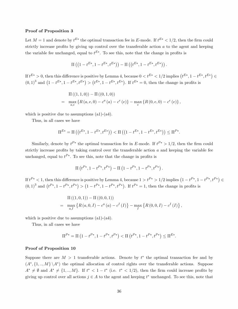
Proof of Proposition 3

Let M = 1 and denote by tE∗ the optimal transaction fee in E-mode. If tE∗ < 1/2, then the firm could

strictly increase profits by giving up control over the transferable action a to the agent and keeping

the variable fee unchanged, equal to tE∗. To see this, note that the change in profits is

Π((

1− tE∗, 1− tE∗, tE∗))−Π

((tE∗, 1− tE∗, tE∗

)).

If tE∗ > 0, then this difference is positive by Lemma 4, because 0 < tE∗ < 1/2 implies(tE∗, 1− tE∗, tE∗

)∈

(0, 1)3 and(1− tE∗, 1− tE∗, tE∗

)>(tE∗, 1− tE∗, tE∗

). If tE∗ = 0, then the change in profits is

Π ((1, 1, 0))−Π ((0, 1, 0))

= maxa,e{R (a, e, 0)− ca (a)− ce (e)} −max

e{R (0, e, 0)− ce (e)} ,

which is positive due to assumptions (a1)-(a4).

Thus, in all cases we have

ΠE∗ = Π((tE∗, 1− tE∗, tE∗

))< Π

((1− tE∗, 1− tE∗, tE∗

))≤ ΠP∗.

Similarly, denote by tP∗ the optimal transaction fee in E-mode. If tP∗ > 1/2, then the firm could

strictly increase profits by taking control over the transferable action a and keeping the variable fee

unchanged, equal to tP∗. To see this, note that the change in profits is

Π(tP∗, 1− tP∗, tP∗

)−Π

(1− tP∗, 1− tP∗, tP∗

).

If tP∗ < 1, then this difference is positive by Lemma 4, because 1 > tP∗ > 1/2 implies(1− tP∗, 1− tP∗, tP∗

)∈

(0, 1)3 and(tP∗, 1− tP∗, tP∗

)>(1− tP∗, 1− tP∗, tP∗

). If tP∗ = 1, then the change in profits is

Π ((1, 0, 1))−Π ((0, 0, 1))

= maxa,I

{R (a, 0, I)− ca (a)− cI (I)

}−max

I

{R (0, 0, I)− cI (I)

},

which is positive due to assumptions (a1)-(a4).

Thus, in all cases we have

ΠP∗ = Π(1− tP∗, 1− tP∗, tP∗

)< Π

(tP∗, 1− tP∗, tP∗

)≤ ΠE∗.

Proof of Proposition 10

Suppose there are M > 1 transferable actions. Denote by t∗ the optimal transaction fee and by

(A∗, {1, ..,M} \A∗) the optimal allocation of control rights over the transferable actions. Suppose

A∗ 6= ∅ and A∗ 6= {1, ..,M}. If t∗ < 1 − t∗ (i.e. t∗ < 1/2), then the firm could increase profits by

giving up control over all actions j ∈ A to the agent and keeping t∗ unchanged. To see this, note that

36

the change in profits is

Π (−→τ (∅, t∗))−Π (−→τ (A∗, t∗)) .

If t∗ > 0, then this difference is positive by Lemma 4, because 1 − t∗ > t∗ > 0 and A∗ 6= ∅ imply−→τ (A∗, t∗) ∈ [0, 1)M+2 and −→τ (∅, t∗) > −→τ (A∗, t∗). If t∗ = 0, then the change in profits can be written

Π (−→τ (∅, 0))−Π (−→τ (A∗, 0)) =

maxa1,..,aM+1

{R(a1, .., aM+1, 0

)−M+1∑i=1

cai (ai)}

−

maxa1,..,aM+1

R (a1, .., aM+1, 0)−

∑i∈{1,..,M+1}\A∗

cai (ai) s.t. ai = 0 if i ∈ A∗

.

Clearly then, A∗ 6= ∅ and assumptions (a1)-(a4) (generalized to the current scenario with multiple

transferable actions) imply Π (−→τ (∅, 0))−Π (−→τ (A∗, 0)) > 0.

Similarly, if t∗ > 1 − t∗, then the firm could increase profits by taking control over all actions

j ∈ {1, ..,M} \A∗ and keeping t∗ unchanged. To see this, note that the change in profits is

Π (−→τ ({1, ..,M} , t∗))−Π (−→τ (A∗, t∗)) .

If t∗ < 1, then this difference is positive by Lemma 4, because 1 > t∗ > 1− t∗ and A∗ 6= {1, ..,M}imply −→τ (A∗, t∗) ∈ [0, 1)M+2 and −→τ ({1, ..,M} , t∗) > −→τ (A∗, t∗). If t∗ = 1, then the change in profits

can be written

Π (−→τ ({1, ..,M} , 1))−Π (−→τ (A∗, 1)) =

maxa1,..,aM ,aM+2

R (a1, .., aM , 0, aM+2)−

∑i∈{1,..,M,M+2}

cai (ai)

−

maxa1,..,aM ,aM+2

R (a1, .., aM , 0, aM+2)−∑

i∈A∗∪{M+2}

cai (ai) s.t. ai = 0 if i ∈ {1, ..,M} \A∗

.

Clearly A∗ 6= {1, ..,M} and assumptions (a1)-(a4) (generalized to the current scenario with multiple

transferable actions) imply Π (−→τ ({1, ..,M} , 1))−Π (−→τ (A∗, 1)) > 0.

Finally, if t∗ = 1/2, then any allocation of control rights yields the same payoffs, so the pure modes

remain weakly optimal.

37