Enabling Validation of a CubeSat Compatible Neutral Wind Sensor

Jon Andrew Williams

Thesis submitted to the faculty of the

Virginia Polytechnic Institute and State University

in partial fulfillment of the requirements for the degree of

Master of Science

In

Electrical Engineering

Gregory D. Earle, Chair

Scott M. Bailey

Wayne A. Scales

June 28, 2017

Blacksburg, VA

Keywords: Retarding Potential Analyzer, Microchannel Plate Detector, Atomic Oxygen, Validation

Copyright © 2017 by Jon Andrew Williams. All rights reserved

Enabling Validation of a CubeSat Compatible Neutral Wind Sensor

Jon Andrew Williams

ABSTRACT The Ram Energy Distribution Detector (REDD) is a new CubeSat-compatible space

science instrument that measures neutral wind characteristics in the upper atmosphere.

Neutral gas interactions with plasma in the ionosphere/thermosphere are responsible for

spacecraft drag, radio frequency disturbances such as scintillation, and other geophysical

phenomena. REDD is designed to collect in-situ measurements within this region of the

atmosphere where in-flight data collection using spacecraft has proven particularly

challenging due to both the atmospheric density and the dominating presence of highly

reactive atomic oxygen (AO). NASA Marshall Space Flight Center has a unique AO

Facility (AOF) capable of simulating the conditions the sensor will encounter on orbit by

creating a supersonic neutral beam of AO. Collimating the beam requires an intense

magnetic field that creates significant interference for sensitive electronic devices. REDD

is undergoing the final stages of validation testing in the AOF. In this presentation, we

describe the LabVIEW-automated system design, the measured geometry and magnitude

of the field, the specially designed mount, and passive shielding that are utilized to

mitigate the effects of the magnetic interference.

Enabling Validation of a CubeSat Compatible Neutral Wind Sensor

Jon Andrew Williams

GENERAL AUDIENCE ABSTRACT The Ram Energy Distribution Detector (REDD) is a new CubeSat-compatible space

science instrument that measures winds in near-Earth space. Gas interactions with plasma

in the upper regions of the atmosphere are responsible for spacecraft drag, radio wave

disturbances, and other phenomena. REDD is designed to collect direct measurements

within this region of the atmosphere where in-flight data collection using conventional

spacecraft has proven particularly challenging. The environmental testing needed to

demonstrate the sensor requires a specialized system located at NASA Marshall Space

Flight Center. To simulate the conditions the sensor will encounter on orbit within a

laboratory requires exposing REDD to a supersonic beam of gas using NASA’s unique

Atomic Oxygen Facility. Forming this gas into a beam requires an intense magnetic field

that creates significant interference for sensors such as REDD. Testing in this facility

requires a specially-designed sensor mount and magnetic shielding system. REDD is

undergoing the final stages of validation testing in the Atomic Oxygen Facility. In this

presentation, we describe the computer software-automated system for testing the sensor,

the shape and strength of the magnetic field, the specially designed sensor mount, and

magnetic shielding that are used to mitigate the effects of the interference.

iv

Dedication To my parents, Harold and Karen Williams for their guidance, advice, and encouragement to pursue my dreams. To Ashley McCormick for her firm support and belief in me. In loving memory of Annie Mae McKeithan and Harold Williams, Sr. without whose influence and belief in advanced education I could not have succeeded.

v

Acknowledgments

I would like to thank to Dr. Gregory D. Earle for his guidance and patience throughout this mentorship. I would also like to give thanks to the Virginia Space Grant Association for its support through the Graduate STEM Research Fellowship Program. A special thanks is due to Stephen Noel for his mentorship, expertise, and invaluable support throughout work on this project. This thesis was completed due to the endless curiosity and previous work of Lee Kordella in advancing the sensor to the prototype stage. A special thanks is due to Curtis Bahr for his patience, humor, tireless devotion to detail, and long hours operating the Atomic Oxygen Facility. This opportunity would not have possible without the mentorship, knowledge, and support of NASA employees Linda Habash-Krause, Dennis Gallagher, and Jason Vaughn. These acknowledgments would not be complete without the work of my colleague Ellen Robertson for her attention to detail, assistance in testing the device, and persistent optimism.

Funding for this research provided by VSGC and NASA MSFC Cooperative Agreement (Sponsor #:NNM16AA11A)

Unless otherwise noted, all photos by author, 2017.

vi

TABLE OF CONTENTS

Introduction ......................................................................................................................... 1

Literature Review................................................................................................................ 3

Background ......................................................................................................................... 5

REDD description ........................................................................................................... 5

AOF Description ............................................................................................................. 8

Magnetic Field Profile of the AOF ................................................................................... 11

Methods, Software, & Apparatus...................................................................................... 21

Hardware – Mount, Passive Shielding, and Interface ................................................... 21

Passive Magnetic Shielding ...................................................................................... 25

Electrical Interface .................................................................................................... 28

Software – REDD Testing GUI .................................................................................... 29

End-to-End Testing ....................................................................................................... 42

Results and Discussion ..................................................................................................... 47

Magnetic Field Mitigation Testing Results .................................................................. 47

End-to-End Testing Results .......................................................................................... 49

Conclusion ........................................................................................................................ 53

Future Work .................................................................................................................. 55

References ......................................................................................................................... 57

Appendix A ....................................................................................................................... 58

Electrical ICD ............................................................................................................... 58

vii

Appendix B ....................................................................................................................... 60

LabVIEW Code: Back End ........................................................................................... 60

viii

LIST OF FIGURES

Figure 1: Side View Cutaway of REDD Cad model, with protective dome shield. ........... 6

Figure 2: Side Views of REDD…………………………………………………………...7

Figure 3: Depicted is an IV curve showing the MCP output current as a function of

extraction plate bias (Earle, 2016). ..................................................................................... 6

Figure 4: The Atomic Oxygen Facility at NASA Marshall Space Flight Center ............... 9

Figure 5: AOF dimensions: side and front views of the AOF with associated axes……10

Figure 6: Original fabricated stand: the original manually adjusted setup for the

kilogauss meter probe ....................................................................................................... 12

Figure 7: Figure 7: Updated probe stand allowing for increased stability and movement

with three degrees of freedom.…………………………………………………………...13

Figure 8: 3-axis MMZ-2502 probe, with XYZ axis orientation. ...................................... 14

Figure 9: Unscaled 3D plot of magnetic flux density within the AOF target cavity. ....... 15

Figure 10: Location of a null point in all three components of the magnetic flux density.

........................................................................................................................................... 16

Figure 11-13: 2D plots of the magnetic flux density component profiles. Comparison

shows a coinciding minimum occurring at approximately 13.25 inches from the origin. 18

Figure 14a and 14b: Optimal location of the most susceptible portion of the REDD device

within the magnetic field………………………………………………………………...20

Figure 15: Custom REDD Mount: Magnetically isolated mounting system for positioning

and testing of the REDD sensor attaches to the standard 8” CF. ...................................... 21

Figure 16: Addition of the 12 inch chamber extension to the AOF chamber. .................. 22

ix

Figure 17: REDD Mounting disk drawing: Autodesk Inventor designed drawing of

mounting disks .................................................................................................................. 23

Figure 18a: Off-axis view of REDD mounting disk Autodesk Inventor 3D CAD model..

........................................................................................................................................... 24

Figure 18b: Side view of REDD mounting disk Autodesk Inventor 3D CAD model. ..... 24

Figure 19a: Inner shielding layer wrapping the REDD sensor ......................................... 26

Figure 19b: Outer cylindrical shielding layer for the REDD sensor ................................ 26

Figure 20: Front view of the passive shielding system for the REDD sensor .................. 27

Figure 21: Rear view of REDD mounting system ............................................................ 28

Figure 22: Flowchart showing dataflow for the LabVIEW Graphic User Interface

(GUI)…………………………………………………………...………………………...32

Figure 23: REDD GUI Front Panel View. ........................................................................ 33

Figure 24: Front panel REDD IV control panel………………………………………….34

Figure 25: Case selector block diagram………………………………………………….35

Figure 26: Vacuum chamber setup for initial aliveness testing conducted at Virginia

Tech................................................................................................................................... 42

Figure 27: COMSOL simulation of estimated particle trajectories and their respective

energies in electron volts (eV), as represented by the color scale situated on the far right.

........................................................................................................................................... 43

Figure 28: Installation of the REDD mounting system onto the 8 inch CF of the AOF

target cavity. ...................................................................................................................... 44

Figure 29: External equipment used in initial end-to-end testing of REDD..................... 45

x

Figure 30: Repeated magnetic field measurements taken after installation of passive

shielding system within the AOF ...................................................................................... 47

Figure 31: Comparison of all three components of the B-field with respect to the location

of REDD within the system .............................................................................................. 48

Figure 32: Initial 8,501 sample capture of the AO pulse using large batch measurements.

........................................................................................................................................... 50

Figure 33: Initial AOF pulse capture. A 39 sample window of MCP output current taken

during the initial 8,501 sample capture of the AO pulse is shown above ......................... 50

Figure 34: Sweep mode functionality test of background gases present in the AOF with

the AO beam disengaged .................................................................................................. 51

Figure 35a: Example of the formatted file output for the Initial Value Cluster panel

populated with user-specified values and comments. ...................................................... 52

Figure 35b: Example of the formatted file output of the REDD GUI .............................. 52

Figure 36: Photograph of a 5eV pulsed AO beam seen during operation of the MSFC

AOF................................................................................................................................... 53

Figure 37: Photograph of REDD GUI during operation ................................................... 55

Figure B1: Method for monitoring temperature through the built-in KE2000 VI. ........... 60

Figure B2: The alteration to Keithley 6517b’s standard Trace Buffer VI……………….60

Figure B3: Signal routing to Current vs Time Plot from the IV Control panel………….61

Figure B4: Signal routing for Real-time I-V plotting ....................................................... 61

xi

LIST OF TABLES

Table 4.1: Initial measured magnetic field measurements within the AOF. .................... 14

Table 4.2: Calculated values for Larmor radius of an AO ion and ratio of instrument

length to this Larmor radius at 293 Kelvin. ...................................................................... 17

Table 5.1: Real-time displays and their associated descriptions. ...................................... 35

Table 5.2: Comparison of Initial approximated coefficients vs calculator-modeled

coefficients ........................................................................................................................ 38

xii

LIST OF ABBREVIATIONS

AO = atomic oxygen

AOF = atomic oxygen facility

REDD = Ram Energy Distribution Detector (pronounced “RED-dee”)

TRL = Technology Readiness Level

LEO = low earth orbit

RWS = Ram Wind Sensor

C/NOFS = Communication/Navigation Outage Forecast System

dt = time step

eV = electron volt

RPA = retarding potential analyzer

MCP = microchannel plate

Bx = X component of the magnetic flux density measured by the probe

By = Y component of the magnetic flux density measured by the probe

Bz = Z component of the magnetic flux density measured by the probe

DI = deionized

GUI = graphical user interface

I/O = input/output

VI = virtual instrument

TDMS = technical data management structure

1

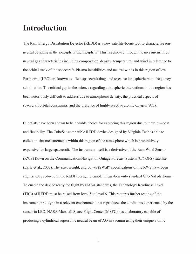
Introduction

The Ram Energy Distribution Detector (REDD) is a new satellite-borne tool to characterize ion-

neutral coupling in the ionosphere/thermosphere. This is achieved through the measurement of

neutral gas characteristics including composition, density, temperature, and wind in reference to

the orbital track of the spacecraft. Plasma instabilities and neutral winds in this region of low

Earth orbit (LEO) are known to affect spacecraft drag, and to cause ionospheric radio frequency

scintillation. The critical gap in the science regarding atmospheric interactions in this region has

been notoriously difficult to address due to atmospheric density, the practical aspects of

spacecraft orbital constraints, and the presence of highly reactive atomic oxygen (AO).

CubeSats have been shown to be a viable choice for exploring this region due to their low-cost

and flexibility. The CubeSat-compatible REDD device designed by Virginia Tech is able to

collect in-situ measurements within this region of the atmosphere which is prohibitively

expensive for large spacecraft. The instrument itself is a derivative of the Ram Wind Sensor

(RWS) flown on the Communication/Navigation Outage Forecast System (C/NOFS) satellite

(Earle et al., 2007). The size, weight, and power (SWaP) specifications of the RWS have been

significantly reduced in the REDD design to enable integration onto standard CubeSat platforms.

To enable the device ready for flight by NASA standards, the Technology Readiness Level

(TRL) of REDD must be raised from level 5 to level 6. This requires further testing of the

instrument prototype in a relevant environment that reproduces the conditions experienced by the

sensor in LEO. NASA Marshall Space Flight Center (MSFC) has a laboratory capable of

producing a cylindrical supersonic neutral beam of AO in vacuum using their unique atomic

2

oxygen facility (AOF). Collimating the beam requires an intense 4 kG magnetic field that creates

significant magnetic interference for sensitive electronics and the flow of charged particles

(Cuthbertson, et al., 1990). REDD is undergoing validation testing in the AOF. In this

presentation, we describe the LabVIEW-automated system design, as well as a specially

designed mount and passive shielding that are utilized to mitigate the effects of the magnetic

interference to enable validation.

3

Literature Review

The following literature review details concepts that were important to developing a testing

system to enable validation of the REDD sensor. It includes review of previous uses of the

MSFC AOF system, and a basic diagram of the device. This is followed by a brief review of the

RWS and its parentage to the REDD sensor. Lastly, this review will discuss previous progress in

prototyping and testing the sensor up to the commencement of this project.

The AOF project at MSFC was begun as a method of producing beams of low energy 3-10 eV

neutral atomic for accelerated material testing at Princeton Plasma Physics Laboratory

(Cuthbertson et al., 1991). This collaboration between NASA MSFC and the Princeton Physics

Department was intended to reproduce the exposure of 5 eV atomic oxygen seen in the LEO

environment. This method of performing surface modification studies proved notably successful

in simulating the erosion of materials such as Kapton in comparison with Flight experiments

aboard STS-8 and STS-41G (Vaughn, et at., 1991). According to plasma emission spectra

recorded during the experiments the oxygen molecules experienced nearly complete dissociation

into atomic oxygen ions. Composition of the AO beam has been verified through mass

spectroscopy and high flux rates of 1016 cm-2s-1 at targets 9 cm from the neutralizer plate were

determined through the use of catalytic probe and material mass loss data. This experimental

facility constructed at Princeton under NASA contract was successful enough to warrant the

creation of MSFC’s own AOF based on this model. The AOF’s remarkable capability to

simulate extended orbital exposure to 5 eV AO plasma is an essential component in the relevant

environmental testing needed to validate the REDD device.

4

REDD’s parentage can be traced to the RWS flown on the C/NOFS satellite from 2008 to 2015.

The RWS is intended to study neutral gas characteristics that signal ionospheric plasma

irregularities responsible for high frequency radio wave disruption. The device was tested

through exposing the device to supersonic fluxes of neutral gas at a specialized facility (Earle, et

al., 2007). The RWS’s main structural elements include an aperture designed to limit incoming

gas particles to a near-normal angle of incidence relative to the spacecraft, charged plates to filter

positive ions and electrons, followed by a grid stack. The electroformed meshes that comprise

the grid stack function as a retarding potential analyzer (RPA) that’s use in ionospheric science

has been well documented in Knudsen’s 1966 paper regarding this device. The number of ions

incident on the channel electron multiplier corresponds proportionally to an output current

experienced by the collecting plate (Earle, et al., 2007). This current is measured as a function of

the retarding voltage applied to one of the grids within the stack and the resulting I-V curve

analyzed using Knudsen’s technique. This method of measuring neutral wind characteristics was

shown to provide a valuable contribution to exploring variation in ionospheric parameters.

Previous design, fabrication, and testing of the REDD prototype were performed in conjunction

with the Creare firm. Without this prior work the current project would not be possible. CAD

models of the system were developed iteratively before the various designs were evaluated using

the SIMION particle trajectory simulator (Earle, 2015). Iterative simulations of the finalized

mechanical design were performed before a prototype device was fabricated and assembled. The

prototype underwent extensive in-vacuum subsystem testing followed by static tests of the

device using an ion source to verify MCP current scaled as a function of chamber pressure. End-

to-end testing of the device was not available without a supersonic neutral gas beam.

5

Background

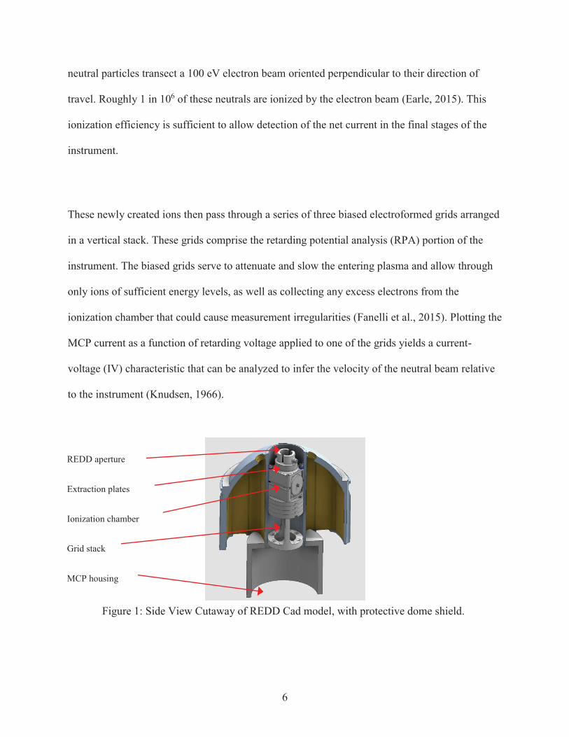
REDD Description The REDD sensor has five key subsystems shown Figure 1: the aperture, extraction plates,

ionization chamber, retarding potential analyzer (RPA) grid stack, and the microchannel plate

(MCP) . The MCP acts as an electron multiplier (Kordella et al., 2016) to boost the signals to

acceptable levels for subsequent analysis. REDD has been designed to admit a supersonic neutral

gas beam approaching 7.8 m/s through the aperture, which is ram-facing to ensure that the beam

enters at near normal incidence relative to the forward-most plane of the spacecraft. As the

neutrals, ions, and electrons enter the aperture at orbital velocity, only the neutrals within the

stream are allowed to reach the ionization chamber within the REDD system because the

electrically biased extraction plates remove ions and electrons from the incident stream of

particles. The extraction plates are located directly behind the aperture, and are biased to ±15

Volts (V) respectively in order to extract the charged particles. Iterative testing in vacuum at

fixed pressure showed that these plate voltages are sufficient to prevent the oxygen ions traveling

at orbital speed from entering the system. 15 V was found to prevent ~200 eV thermal electrons,

and ~5eV positive ions, from biasing the MCP current measurements. The neutral gas

components are impervious to the potentials on the extraction plates, and since the mean free

path of the particles is large relative to the instrument, the neutrals will continue past the plates

and into the ionization chamber.

The geometry of the instrument aperture and the internal ionization chamber aperture ensure that

a collimated beam of neutrals is admitted to the ionization chamber. Within this chamber the

6

neutral particles transect a 100 eV electron beam oriented perpendicular to their direction of

travel. Roughly 1 in 106 of these neutrals are ionized by the electron beam (Earle, 2015). This

ionization efficiency is sufficient to allow detection of the net current in the final stages of the

instrument.

These newly created ions then pass through a series of three biased electroformed grids arranged

in a vertical stack. These grids comprise the retarding potential analysis (RPA) portion of the

instrument. The biased grids serve to attenuate and slow the entering plasma and allow through

only ions of sufficient energy levels, as well as collecting any excess electrons from the

ionization chamber that could cause measurement irregularities (Fanelli et al., 2015). Plotting the

MCP current as a function of retarding voltage applied to one of the grids yields a current-

voltage (IV) characteristic that can be analyzed to infer the velocity of the neutral beam relative

to the instrument (Knudsen, 1966).

REDD aperture Extraction plates Ionization chamber Grid stack MCP housing

Figure 1: Side View Cutaway of REDD Cad model, with protective dome shield.

7

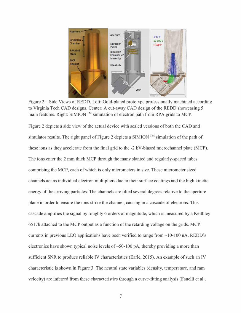
Figure 2 – Side Views of REDD. Left: Gold-plated prototype professionally machined according to Virginia Tech CAD designs. Center: A cut-away CAD design of the REDD showcasing 5 main features. Right: SIMION TM simulation of electron path from RPA grids to MCP.

Figure 2 depicts a side view of the actual device with scaled versions of both the CAD and

simulator results. The right panel of Figure 2 depicts a SIMION TM simulation of the path of

these ions as they accelerate from the final grid to the -2 kV-biased microchannel plate (MCP).

The ions enter the 2 mm thick MCP through the many slanted and regularly-spaced tubes

comprising the MCP, each of which is only micrometers in size. These micrometer sized

channels act as individual electron multipliers due to their surface coatings and the high kinetic

energy of the arriving particles. The channels are tilted several degrees relative to the aperture

plane in order to ensure the ions strike the channel, causing in a cascade of electrons. This

cascade amplifies the signal by roughly 6 orders of magnitude, which is measured by a Keithley

6517b attached to the MCP output as a function of the retarding voltage on the grids. MCP

currents in previous LEO applications have been verified to range from ~10-100 nA. REDD’s

electronics have shown typical noise levels of ~50-100 pA, thereby providing a more than

sufficient SNR to produce reliable IV characteristics (Earle, 2015). An example of such an IV

characteristic is shown in Figure 3. The neutral state variables (density, temperature, and ram

velocity) are inferred from these characteristics through a curve-fitting analysis (Fanelli et al.,

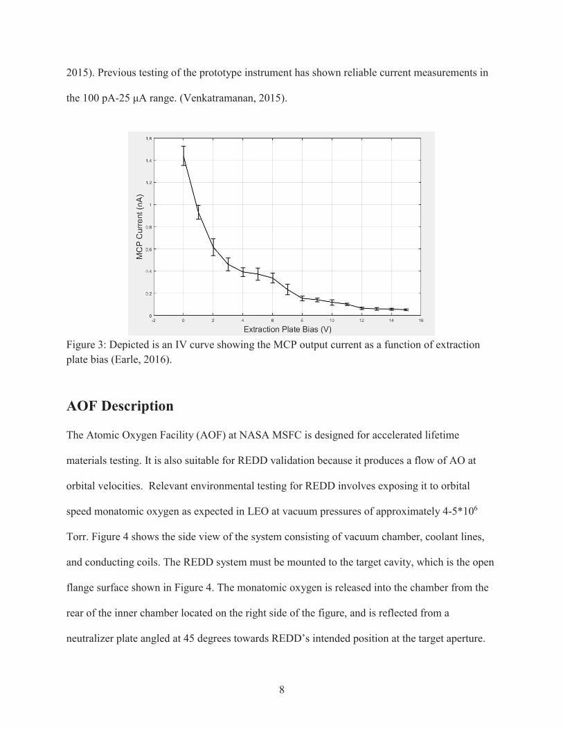
8

2015). Previous testing of the prototype instrument has shown reliable current measurements in

the 100 pA-25 μA range. (Venkatramanan, 2015).

Figure 3: Depicted is an IV curve showing the MCP output current as a function of extraction plate bias (Earle, 2016).

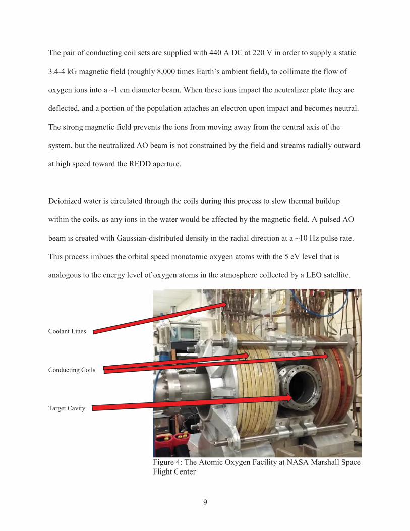
AOF Description The Atomic Oxygen Facility (AOF) at NASA MSFC is designed for accelerated lifetime

materials testing. It is also suitable for REDD validation because it produces a flow of AO at

orbital velocities. Relevant environmental testing for REDD involves exposing it to orbital

speed monatomic oxygen as expected in LEO at vacuum pressures of approximately 4-5*106

Torr. Figure 4 shows the side view of the system consisting of vacuum chamber, coolant lines,

and conducting coils. The REDD system must be mounted to the target cavity, which is the open

flange surface shown in Figure 4. The monatomic oxygen is released into the chamber from the

rear of the inner chamber located on the right side of the figure, and is reflected from a

neutralizer plate angled at 45 degrees towards REDD’s intended position at the target aperture.

9

The pair of conducting coil sets are supplied with 440 A DC at 220 V in order to supply a static

3.4-4 kG magnetic field (roughly 8,000 times Earth’s ambient field), to collimate the flow of

oxygen ions into a ~1 cm diameter beam. When these ions impact the neutralizer plate they are

deflected, and a portion of the population attaches an electron upon impact and becomes neutral.

The strong magnetic field prevents the ions from moving away from the central axis of the

system, but the neutralized AO beam is not constrained by the field and streams radially outward

at high speed toward the REDD aperture.

Deionized water is circulated through the coils during this process to slow thermal buildup

within the coils, as any ions in the water would be affected by the magnetic field. A pulsed AO

beam is created with Gaussian-distributed density in the radial direction at a ~10 Hz pulse rate.

This process imbues the orbital speed monatomic oxygen atoms with the 5 eV level that is

analogous to the energy level of oxygen atoms in the atmosphere collected by a LEO satellite.

Coolant Lines Conducting Coils

Target Cavity

Figure 4: The Atomic Oxygen Facility at NASA Marshall Space Flight Center

10

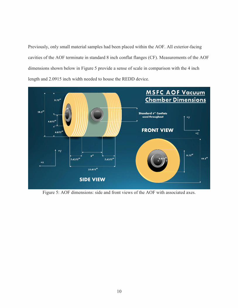
Previously, only small material samples had been placed within the AOF. All exterior-facing

cavities of the AOF terminate in standard 8 inch conflat flanges (CF). Measurements of the AOF

dimensions shown below in Figure 5 provide a sense of scale in comparison with the 4 inch

length and 2.0915 inch width needed to house the REDD device.

Figure 5: AOF dimensions: side and front views of the AOF with associated axes.

11

Magnetic Field Profile of the AOF

In order to utilize the AOF at MSFC for validation testing of the REDD instrument it is

necessary to know the magnetic field geometry and magnitude within the testing chamber. The

peak value of the magnetic field at the center of the chamber is known to be ~4 kG (Cuthbertson,

et al., 1991). The field is expected to be solenoidal because it is produced by a symmetric coil

system along the cylindrical axis of the vacuum chamber. A 4 kG field will have significant

effects on the paths of the electrons emitted by the filament and on the trajectories of ions

traveling through the device. The expected current output of the MCP is in the nA - μA range

(Earle, 2016), and the pertubations caused by the magnetic field would render current

measurements unreliable under these conditions. Validation testing in this environment therefore

requires magnetic shielding at the location of a minimum in the solenoidal magnetic field.

A Lakeshore Model 460 kilogauss meter with a 3-axis transverse probe is used to provide

accurate measurements of all three magnetic field components simultaneously. The meter

provides a calculated magnitude as well. According to the datasheet, the Model 460 Hall effect

gaussmeter is able to measure fields of 300 mG – 300 kG at an overall rated DC accuracy of

0.1% of reading. The 2.125 inch MMZ-2502-UH probe is utilized for its 30 kG range with an

accuracy of 0.25% at 25° C with 5 digits of precision. The probe was calibrated using the

included Lakeshore zero-gauss block. The magnitude of the Earth ambient field at room

temperature within the MSFC laboratory containing the AOF has been previously measured to

be 0.4-0.5 G, which was verified by the Model 460 reading of 0.412 G after calibration.

12

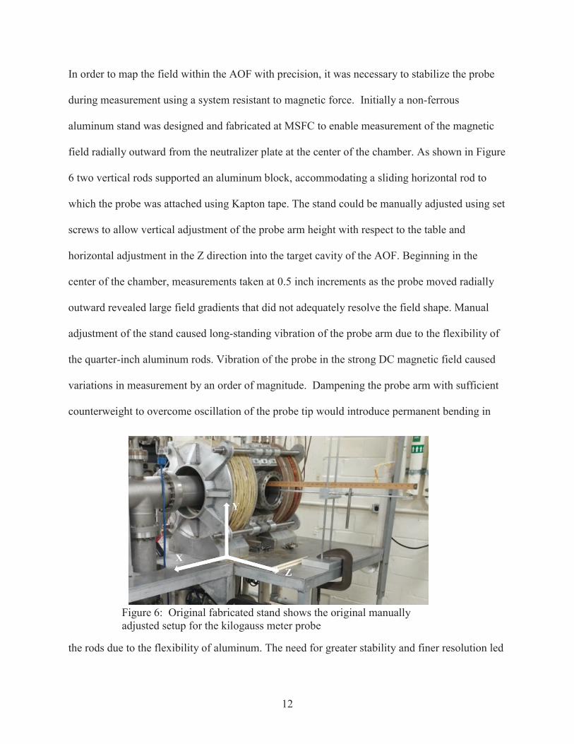
In order to map the field within the AOF with precision, it was necessary to stabilize the probe

during measurement using a system resistant to magnetic force. Initially a non-ferrous

aluminum stand was designed and fabricated at MSFC to enable measurement of the magnetic

field radially outward from the neutralizer plate at the center of the chamber. As shown in Figure

6 two vertical rods supported an aluminum block, accommodating a sliding horizontal rod to

which the probe was attached using Kapton tape. The stand could be manually adjusted using set

screws to allow vertical adjustment of the probe arm height with respect to the table and

horizontal adjustment in the Z direction into the target cavity of the AOF. Beginning in the

center of the chamber, measurements taken at 0.5 inch increments as the probe moved radially

outward revealed large field gradients that did not adequately resolve the field shape. Manual

adjustment of the stand caused long-standing vibration of the probe arm due to the flexibility of

the quarter-inch aluminum rods. Vibration of the probe in the strong DC magnetic field caused

variations in measurement by an order of magnitude. Dampening the probe arm with sufficient

counterweight to overcome oscillation of the probe tip would introduce permanent bending in

the rods due to the flexibility of aluminum. The need for greater stability and finer resolution led

Figure 6: Original fabricated stand shows the original manually adjusted setup for the kilogauss meter probe

13

to the construction and use of the stand in Figure 7 with the assistance of facility operator, Curtis

Bahr. The new rigid stand increases stability significantly and allows for refined adjustment of

the probe location with three degrees of freedom and 0.0625 inch resolution. A rail allows for

smooth linear movement in the z-direction, but is limited to 15 inches radially outward from the

neutralizer plate at the center of the AOF’s vacuum chamber. The new design retains the non-

ferrous quarter-inch aluminum rod to which the probe is mounted.

Figure 7: Updated probe stand allowing for increased stability and movement with three degrees of freedom

14

Location of probe measurements of the AOF magnetic field vector components and magnitude

are taken with respect to the chamber center where the field magnitude has been previously

verified (Vaughn et al., 1991). Orientation of the transverse probe and its associated

measurement axes are shown in Figure 8. The X-axis is aligned with the AO beam’s direction of

travel and coincides with the longitudinal X axis of the coils, while Y and Z axis respectively

coincide with transverse axes. Initial measurements in Table 4.1 show that the field magnitude at

the location of the neutralizer plate is accurate in comparison to previous measurements

considering ambient temperature of the coils and aging of the system (personal communication,

Curtis Bahr).

Table 4.1: Initial measured magnetic field measurements within the AOF.

Measured Field at AOF Center

X Y Z XYZ Magnitude

Ambient Field 0.144 G 0.216 G 0.320 G 0.412 G AOF field activated 3.342 kG 151.14 G 110.19 G 3.347 kG

To locate a local minimum and establish a detailed profile both the shape and magnitude of the

field are desired. Further in-situ field measurements were taken at the target cavity, extending 15

inches radially outward from center in increments of 0.25 inches (in the Z direction). Each trial

Figure 8: 3-axis MMZ-2502-UH probe, with XYZ axis orientation

15

consists of five sets of radial measurements as shown in Figure 9: centered within the target

cavity and aligned with the axis of the AO beam, ±1 inch in the Y-direction, and ±1 inch in the

X-direction. The XYZ location with respect to the center of the AOF was recorded with each

measurement, along with the respective component and magnitude values. The magnetic flux

density depicted at each increment in Figure 9 is depicted as a vector that points primarily in the

x-direction with a length proportional to the vector magnitude calculated by the kilogauss meter.

It should be noted that Bx, which lies along the cylindrical axis of the coils, dominates both the

Y and Z components of the field for the large majority of the measurement trials. Nullifying this

Figure 9: Unscaled 3D plot of magnetic flux density within the AOF target cavity. The relative length of the magnetic flux density vectors indicate the magnitude of the field strength. Each set of vectors represents measurements taken radially outward from the AOF center along the transverse Z axis during five separate trials centered at different positions.

16

X component of the magnetic flux density is identified as the main factor in mitigating any

magnetic interference with the charged particles traveling within the REDD device.

These resulting measurement profiles were repeated and confirmed by the MSFC AOF

technician in a separate trial. Each set of measurements confirm the existence of a null point in

all three components of the magnetic flux density coinciding at the probe position shown in

Figure 10. This null point is located 13.25 inches radially outward in the Z direction and is

centered on the X-Y axes relative to the chamber center. It resides in the area 1.25 inches outside

the target cavity where the polarity of the field changes in the Bx and By components. Figure 11

shows a comparison of the respective 2D magnetic flux density plots and reveals a coinciding

minimum for Bx, By, and Bz. Field strength in all three components of the magnetic field at this

Figure 10: Location of a null point in all three components of the magnetic flux density.

17

location were measured to be at Earth ambient levels over a range of ~0.25 inches in the Z

direction.

The measured values of magnetic flux density would have significant effects on the charged

particles traveling through the REDD device. Particles moving perpendicular to a static magnetic

field will move in circular orbits with a constant radius, called the Larmor radius. The form of

Larmor radius used is given by the Equation (1) (Bittencourt 2013).

In order to minimize magnetic interference during the operation of REDD, the desired Larmor

radius of charged particles traveling through the device should exceed 10-100 times the 9.403 cm

length of the device. Table 4.2 illustrates the dominant effect of Bx, with magnitudes greater than

13.7 G causing charged particles to collide with the interior of the cylindrical sheath before

reaching the MCP at the rear of the device.

Table 4.2: Calculated values for Larmor radius of an AO ion and ratio of instrument length to this Larmor radius at 293 Kelvin.

Bx RL Instrument Length / RL 0.5 G 25.87 m 275.12 1.37 G 9.44 m 100.4 13.7 G 94.43 cm 10.04 30 G 43.11 cm 4.59 300 G 4.31 cm 0.459

18

Figure 11-13: 2D plots of the magnetic flux density component profiles. Comparison shows a coinciding minimum occurring at approximately 13.25 inches from the origin.

19

The portion of the REDD device that is most sensitive to magnetic interference is the ~2 inch

path travelled by AO ions from the ionization chamber to the MCP. Optimally, the minimum of

the Bx and By components of the magnetic field should be located in this area. The change in

polarity of the field after this null point in both the X and Y directions further ensures that

charged particles do not collide with the interior walls of the device before reaching the MCP

detector. Figures 15 and 16 depict this optimal location of REDD’s most susceptible area within

the magnetic field profile of the AOF from two respective viewpoints. In order to reduce the

possibility of interference with the device, this sensitive area should be centered on the location

of minimum magnetic flux density magnitude.

20

Figure 14a and 14b: Optimal location of the most susceptible portion of the REDD device within the magnetic field.

21

Methods, Software, & Apparatus

Hardware – Mount, Passive Shielding, and Interface

End-to-end testing of the REDD sensor in a relevant environment requires positioning the device

with the aperture facing normal to the flow of the beam. Optimal placement of the device is

aligned with the center of the beam that flows radially outward from the center of the chamber.

Though both the flux and fluence rates of the system are known to the highest degree of

accuracy at this location in the center of the chamber, REDD cannot be placed there as doing so

would result in the very highest levels of magnetic interference. As previously stated, accurate

and adjustable positioning of REDD is vital to testing the sensor within the AOF’s intense

magnetic field. In addition, μ-metal sheets are used to attenuate the field. Mounting the sensor at

the location of the null point 13.25 inches from the chamber center requires modification of the

system through the addition of a 12 inch extension in the radial direction, as this position lies

Figure 15: Custom REDD Mount: Magnetically isolated mounting system for positioning and testing of the REDD sensor attaches to the standard 8” CF.

22

outside the original target cavity as seen in Figure 16. Probe measurements were repeated to

confirm this alteration to the chamber did not cause any significant changes to the magnetic

geometry or magnitude of the field profile.

Figure 16: Addition of the 12 inch chamber extension to the AOF chamber. Magnetic field measurements along the beam’s axis were repeated to ensure the integrity of the field geometry and magnitude.

23

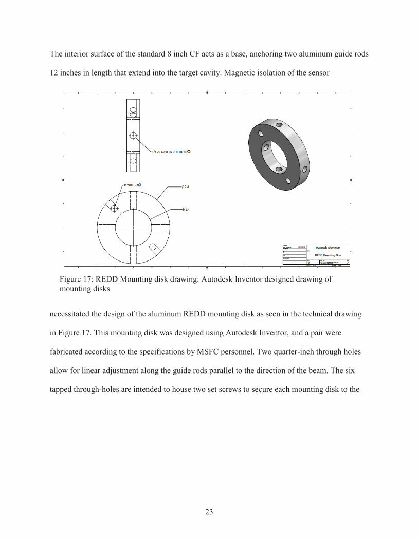
The interior surface of the standard 8 inch CF acts as a base, anchoring two aluminum guide rods

12 inches in length that extend into the target cavity. Magnetic isolation of the sensor

necessitated the design of the aluminum REDD mounting disk as seen in the technical drawing

in Figure 17. This mounting disk was designed using Autodesk Inventor, and a pair were

fabricated according to the specifications by MSFC personnel. Two quarter-inch through holes

allow for linear adjustment along the guide rods parallel to the direction of the beam. The six

tapped through-holes are intended to house two set screws to secure each mounting disk to the

Figure 17: REDD Mounting disk drawing: Autodesk Inventor designed drawing of mounting disks

24

guide rods and four to house nylon set screws for securing the sensor within the interior of the

disks. The configuration is shown in Figures 18a and 18b. These nylon screws allow for

stabilization and accurate alignment of REDD with the beam’s angle of arrival while providing

the necessary magnetic isolation of the device from the aluminum disks and guide rods. Four

Figure 18a: Off-axis view of REDD mounting disk Autodesk Inventor 3D CAD model. Scale REDD sensor situated at the intended position within the disks for reference.

Figure 18b: Side view of REDD mounting disk Autodesk Inventor 3D CAD model. Scale REDD sensor situated at the intended position within the disks for reference.

25

cavities extending through the CF base provide access to the needed connectors for operating

and monitoring the REDD sensor.

Passive Magnetic Shielding

The main feature of the mount is the passive shielding system consisting of two concentric

cylinders of μ-metal encasing the REDD sensor that are used to attenuate the field at this

position and shield the device. The use of multiple shielding layers is due to the difficultly in

reaching high shielding factors without reaching magnetic saturation in a single layer (Mager,

1970). Equation (1) was used to test the hypothesis that two concentric layers of shielding would

be sufficient to suppress field magnitudes to approximately Earth ambient levels at the location

of the REDD sensor (Personal communications, Dr. Ahmad Safaai-Jazi).

Where is the approximate permeability of the μ-metal, is the maximum field to be

attenuated, and a/b represents the wall thickness ratio of the shields used. Using an estimated

80,000 for the permeability, 4000 G as the maximum field, and thickness ratio of ~1 to represent

thin shields, the calculated field value with two cylindrical shield layers was calculated to be

4.847 G. Field magnitudes of this level were shown to be sufficient using Table 4.1 Wrapping

each cylindrical layer multiple times was theorized to decrease this value further and guarantee

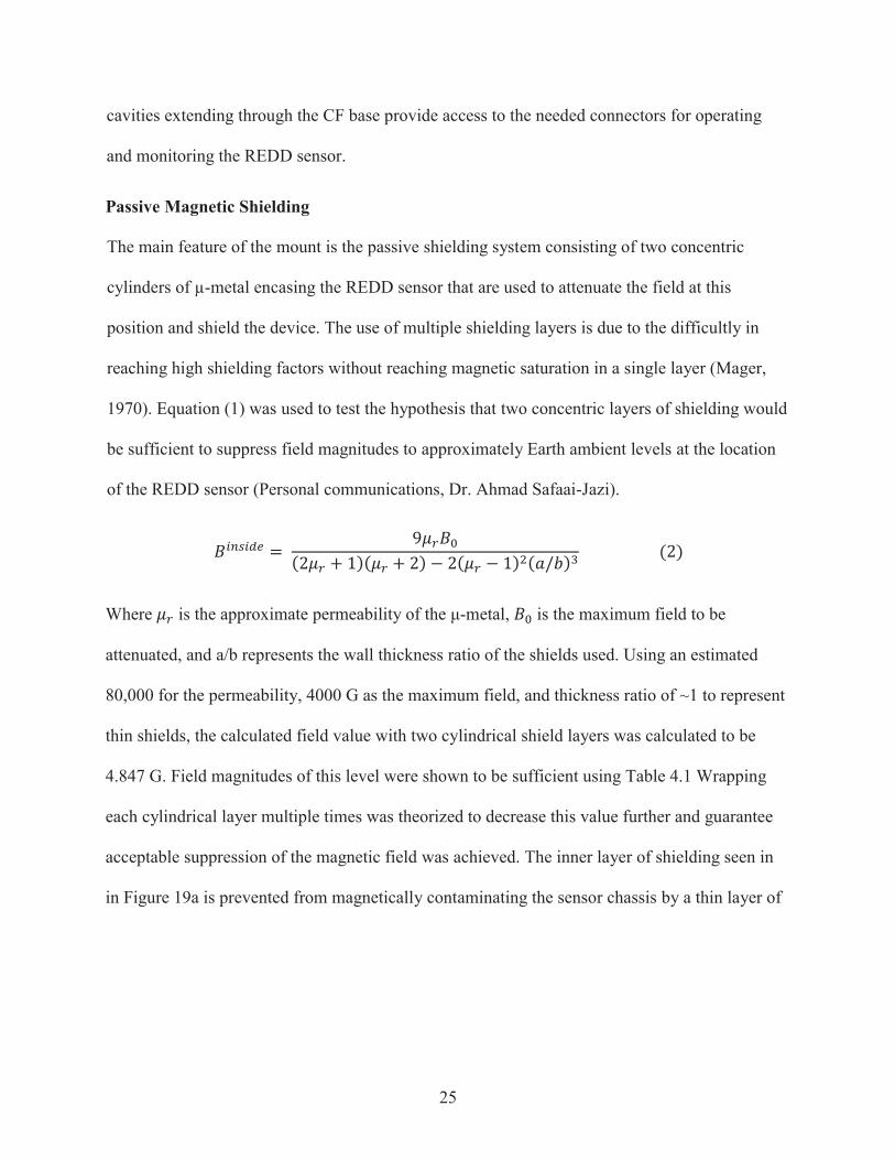
acceptable suppression of the magnetic field was achieved. The inner layer of shielding seen in

in Figure 19a is prevented from magnetically contaminating the sensor chassis by a thin layer of

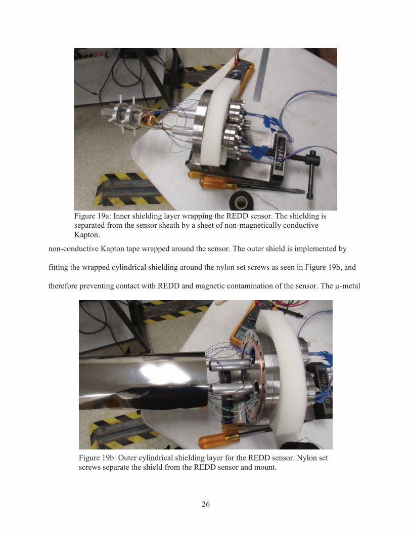
26

non-conductive Kapton tape wrapped around the sensor. The outer shield is implemented by

fitting the wrapped cylindrical shielding around the nylon set screws as seen in Figure 19b, and

therefore preventing contact with REDD and magnetic contamination of the sensor. The μ-metal

Figure 19a: Inner shielding layer wrapping the REDD sensor. The shielding is separated from the sensor sheath by a sheet of non-magnetically conductive Kapton.

Figure 19b: Outer cylindrical shielding layer for the REDD sensor. Nylon set screws separate the shield from the REDD sensor and mount.

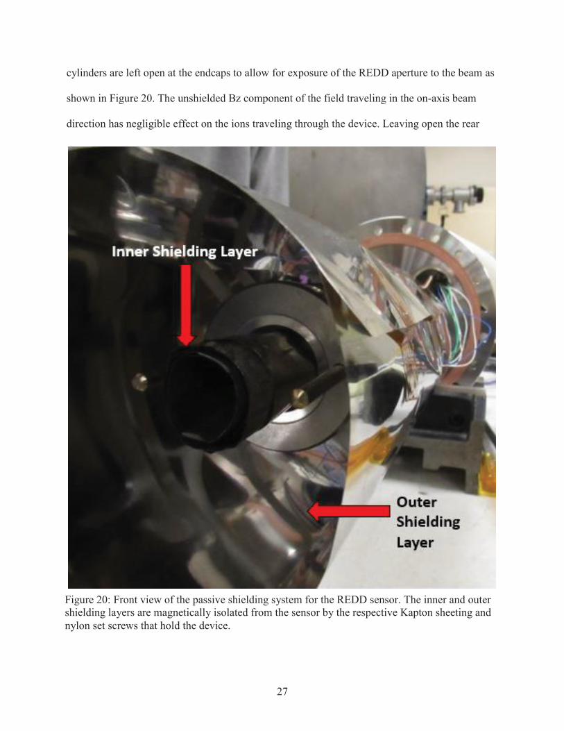
27

cylinders are left open at the endcaps to allow for exposure of the REDD aperture to the beam as

shown in Figure 20. The unshielded Bz component of the field traveling in the on-axis beam

direction has negligible effect on the ions traveling through the device. Leaving open the rear

Figure 20: Front view of the passive shielding system for the REDD sensor. The inner and outer shielding layers are magnetically isolated from the sensor by the respective Kapton sheeting and nylon set screws that hold the device.

28

endcaps allows for the trailing wires to be threaded into four cavities leading to the respective

vacuum-safe connectors.

Electrical Interface

These cavities terminate in four 2.75 inch CF’s that house four distinct feedthroughs, as seen in

Figure 21. This interface consists of two vacuum-safe DB-9 connectors, one BNC connector for

MCP output, and four available high voltage pins. The inclusion of additional connectors and

added pins allows for alternate configurations and expansion of the electrical interface during

future testing. The connectors above lead to the accompanying power supplies, two Keithley

6517b electrometers, and one Keithley 2000 to monitor temperature. A thermistor is attached to

the ionization chamber within REDD using thermally-conductive paste to enable monitoring of

Figure 21: Rear view of REDD mounting system. Four feedthroughs allow for electrical interface between external equipment and the sensor inside the AOF chamber.

29

device temperature. Several material and geometry changes were made during construction and

initial subsystem testing:

1. Tungsten filaments were formerly adopted as the source of electron production in the

ionization chamber.

2. Step 1 facilitated the redesign and fabrication of backing plates responsible for mounting

the filament and enclosing the ionization chamber sidewalls.

3. Aluminum brackets surrounding the ionization chamber were needed for additional heat

sinking to mitigate the possibility of damage to the original Kel-F brackets.

Further electrical connection details concerning the interface, pin-outs, wire gauges, harnesses,

and external equipment are detailed in the electrical ICD included in Appendix A. The Keithley

measurement devices and power supplies necessary for sweeping the retarding grid voltages are

controlled through a LabVIEW graphic user interface (GUI) developed for this purpose.

Software – REDD Testing GUI To automate the test procedure a custom-designed GUI is needed since manual sampling of the

10 Hz AO beam with acceptable resolution is not feasible. The interface allows various

empirical settings to be controlled, and provides feedback to the experimenters that can greatly

improve the efficiency of validation testing. The LabVIEW programmed GUI detailed in this

document is designed to provide a communication interface between the user, the REDD device,

and the associated testing equipment. . The equipment communicates with the software using the

IEEE-488 standard, otherwise known as General Purpose Interface Bus (GPIB). This software

takes user input parameters and interprets the commands of controllable graphical elements in

order to operate the Keithley 6517B, Keithley 2000, and Agilent 6645A. The software has

30

additional functionality that allows for real-time plotting of measurements and parsed data

recording to an output file. The GUI was created and implemented using National Instruments

LabVIEW, Versions 15 and 16.

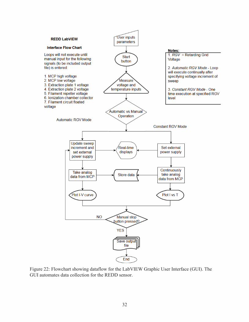
The flowchart of the GUI seen in Figures 22 illustrates the path of data through the program

beginning with initialization and ending with file output. The GUI is manually started,

implements the chosen mode of operation, appropriately commands the external equipment, and

displays the appropriate real-time information before recording data output. The program

features flexible user control for a number of functions including choice of external equipment

roles, mode select, plotting, output file location, and filename. The two modes of operation

consist of a constant voltage mode for debugging and an automated sweep mode. The constant

mode holds the retarding grid voltage at a single level in order to monitor current output, confirm

capture of the pulse, and calibrate the system. The automated sweep mode holds the retarding

grid voltage level for the desired amount of readings before increasing the voltage by user-

specified increments. All data recording is handled by the script through a custom virtual

instrument (VI) module that creates preformatted spreadsheets of the hardware settings and

measurement device outputs in a native format compatible with a standard Microsoft Excel

spreadsheet.

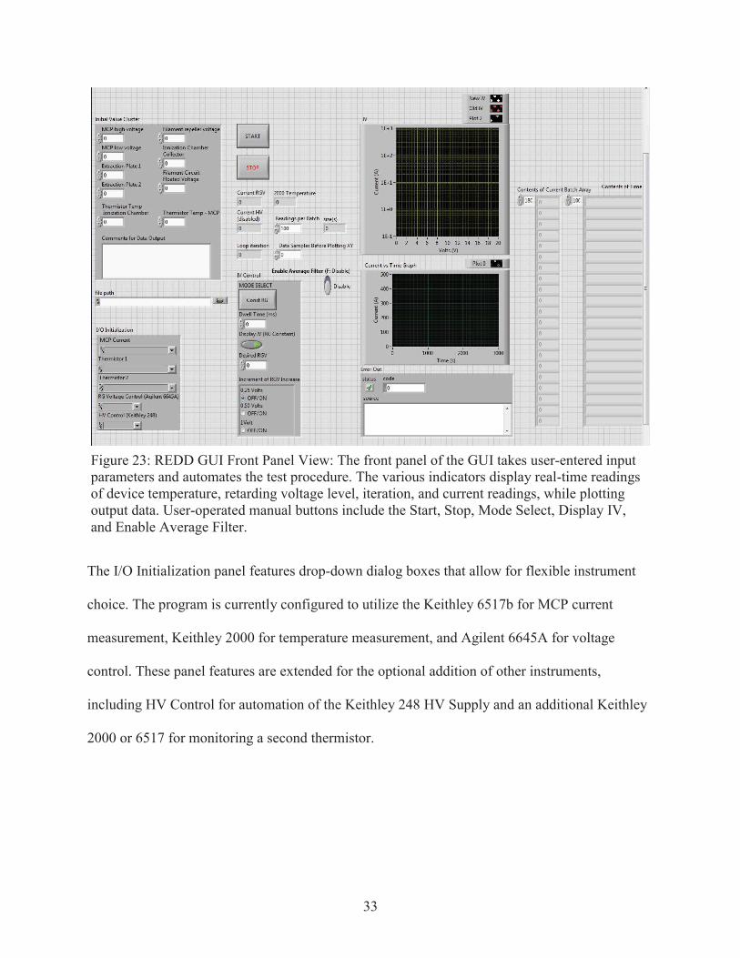
A view of the GUI front panel shown in Figure 23 showcases the various controls and displays

available to the user. This Front End view of the LabVIEW software is intended to represent the

GUI during normal operation while the hidden back end provides direct access to the modules,

31

configurations, virtual wiring, and the more technical coding. Prominent features of the front

panel include:

Input/output (I/O) initialization panel

Manual start and stop buttons

I-V control panel with mode select

Real-time displays of temperature, voltage, iteration, current, and plots

Sample controls for batches and plots

Initial value cluster panel for data record management

32

Figure 22: Flowchart showing dataflow for the LabVIEW Graphic User Interface (GUI). The GUI automates data collection for the REDD sensor.

33

The I/O Initialization panel features drop-down dialog boxes that allow for flexible instrument

choice. The program is currently configured to utilize the Keithley 6517b for MCP current

measurement, Keithley 2000 for temperature measurement, and Agilent 6645A for voltage

control. These panel features are extended for the optional addition of other instruments,

including HV Control for automation of the Keithley 248 HV Supply and an additional Keithley

2000 or 6517 for monitoring a second thermistor.

Figure 23: REDD GUI Front Panel View: The front panel of the GUI takes user-entered input parameters and automates the test procedure. The various indicators display real-time readings of device temperature, retarding voltage level, iteration, and current readings, while plotting output data. User-operated manual buttons include the Start, Stop, Mode Select, Display IV, and Enable Average Filter.

34

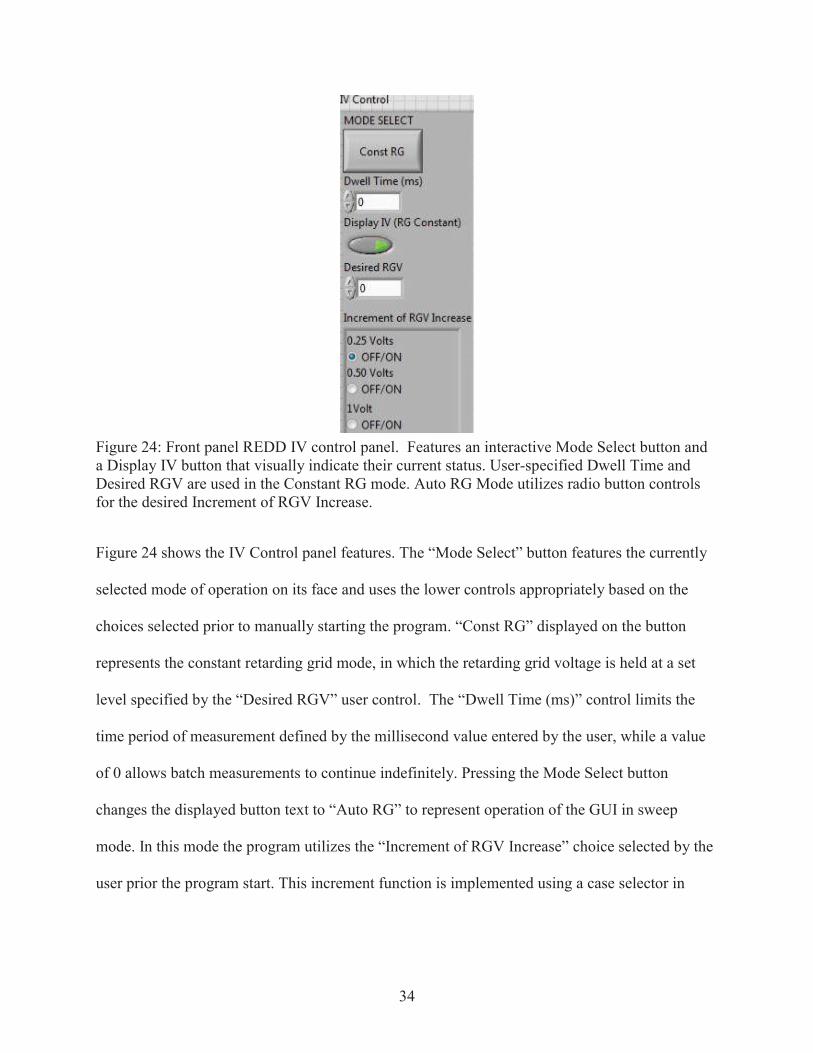
Figure 24 shows the IV Control panel features. The “Mode Select” button features the currently

selected mode of operation on its face and uses the lower controls appropriately based on the

choices selected prior to manually starting the program. “Const RG” displayed on the button

represents the constant retarding grid mode, in which the retarding grid voltage is held at a set

level specified by the “Desired RGV” user control. The “Dwell Time (ms)” control limits the

time period of measurement defined by the millisecond value entered by the user, while a value

of 0 allows batch measurements to continue indefinitely. Pressing the Mode Select button

changes the displayed button text to “Auto RG” to represent operation of the GUI in sweep

mode. In this mode the program utilizes the “Increment of RGV Increase” choice selected by the

user prior the program start. This increment function is implemented using a case selector in

Figure 24: Front panel REDD IV control panel. Features an interactive Mode Select button and a Display IV button that visually indicate their current status. User-specified Dwell Time and Desired RGV are used in the Constant RG mode. Auto RG Mode utilizes radio button controls for the desired Increment of RGV Increase.

35

LabVIEW based upon the diagram shown in Figure 25. Retarding grid voltage level changes

occur after each complete batch of current measurements is taken.

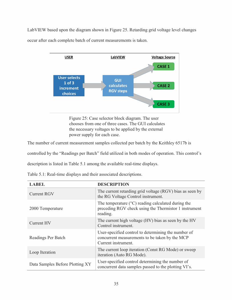
The number of current measurement samples collected per batch by the Keithley 6517b is

controlled by the “Readings per Batch” field utilized in both modes of operation. This control’s

description is listed in Table 5.1 among the available real-time displays.

Table 5.1: Real-time displays and their associated descriptions.

LABEL DESCRIPTION

Current RGV The current retarding grid voltage (RGV) bias as seen by the RG Voltage Control instrument.

2000 Temperature The temperature (°C) reading calculated during the preceding RGV check using the Thermistor 1 instrument reading.

Current HV The current high voltage (HV) bias as seen by the HV Control instrument.

Readings Per Batch User-specified control to determining the number of concurrent measurements to be taken by the MCP Current instrument.

Loop Iteration The current loop iteration (Const RG Mode) or sweep iteration (Auto RG Mode).

Data Samples Before Plotting XY User-specified control determining the number of concurrent data samples passed to the plotting VI’s.

Figure 25: Case selector block diagram. The user chooses from one of three cases. The GUI calculates the necessary voltages to be applied by the external power supply for each case.

36

Batch size and loop iteration are included for debugging purposes to ensure that correctly sized

arrays for measurement batches were created by the program at each iteration. The “Data

Samples Before Plotting XY” control allows for increased GUI performance by limiting point

drawing within the respective plots to occur in batches. This is a necessary addition as lines

drawn using point-at-a-time plotting during 1000 point batches proved particularly taxing on the

GUI’s sample rate. The LabVIEW built-in sub-VI operating the real-time plot windows forces a

new bitmap drawing to the display after each update, slowing batch measurement sample rates

by two thirds in the initial 1000 point batch test. This was overcome by using the Data Samples

Before Plotting XY control to limit the amount of plot updates to user-specified intervals.

Further testing revealed values ranging from a minimum of 10 points to a maximum of the

Readings per Batch value selected by the user. This approach allows for smooth plot formation

with negligible latency.

Monitoring the temperature of the ionization chamber is critical to enabling validation of the

REDD sensor. This chamber houses components supplied with 2 amps of current, which is

necessary for a filament based ionization source. The hot filament that sources the ionizing

electrons poses a risk to non-metallic components in close proximity to the filament. Various

Kel-F components within the device may experience outgassing at temperatures above 90°C, and

the MCP may incur damage or produce inconsistent measurements as a result. The temperature

is monitored by converting the measured variable resistance value of the Honeywell 10K NTC

thermistor into the corresponding temperature. The conversion varies per resistor and the

temperature range of interest. Calibration uses the Steinhart-Hart polynomial coefficients to

37

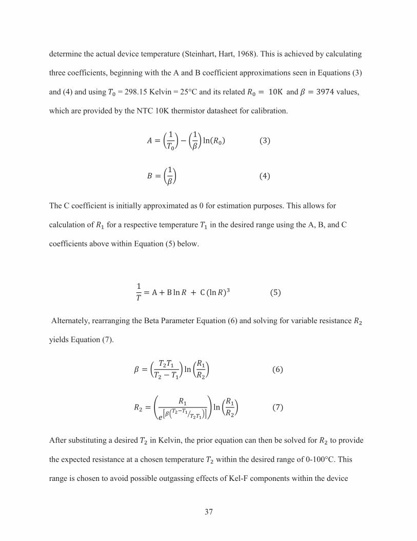
determine the actual device temperature (Steinhart, Hart, 1968). This is achieved by calculating

three coefficients, beginning with the A and B coefficient approximations seen in Equations (3)

and (4) and using = 298.15 Kelvin = 25°C and its related and values,

which are provided by the NTC 10K thermistor datasheet for calibration.

The C coefficient is initially approximated as 0 for estimation purposes. This allows for

calculation of for a respective temperature in the desired range using the A, B, and C

coefficients above within Equation (5) below.

Alternately, rearranging the Beta Parameter Equation (6) and solving for variable resistance

yields Equation (7).

After substituting a desired in Kelvin, the prior equation can then be solved for to provide

the expected resistance at a chosen temperature within the desired range of 0-100°C. This

range is chosen to avoid possible outgassing effects of Kel-F components within the device

38

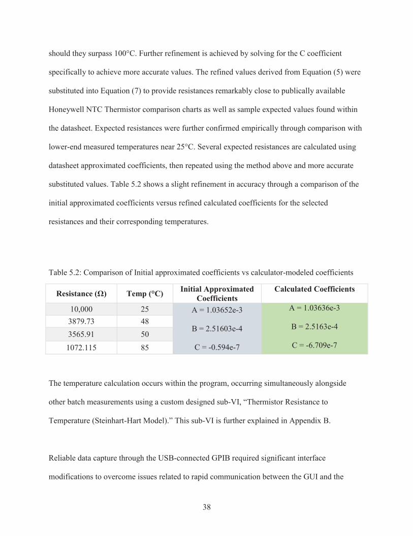
should they surpass 100°C. Further refinement is achieved by solving for the C coefficient

specifically to achieve more accurate values. The refined values derived from Equation (5) were

substituted into Equation (7) to provide resistances remarkably close to publically available

Honeywell NTC Thermistor comparison charts as well as sample expected values found within

the datasheet. Expected resistances were further confirmed empirically through comparison with

lower-end measured temperatures near 25°C. Several expected resistances are calculated using

datasheet approximated coefficients, then repeated using the method above and more accurate

substituted values. Table 5.2 shows a slight refinement in accuracy through a comparison of the

initial approximated coefficients versus refined calculated coefficients for the selected

resistances and their corresponding temperatures.

Table 5.2: Comparison of Initial approximated coefficients vs calculator-modeled coefficients

Resistance (Ω) Temp (°C) Initial Approximated

Coefficients Calculated Coefficients

10,000 25 A = 1.03652e-3

B = 2.51603e-4

C = -0.594e-7

A = 1.03636e-3

B = 2.5163e-4

C = -6.709e-7

3879.73 48 3565.91 50

1072.115 85

The temperature calculation occurs within the program, occurring simultaneously alongside

other batch measurements using a custom designed sub-VI, “Thermistor Resistance to

Temperature (Steinhart-Hart Model).” This sub-VI is further explained in Appendix B.

Reliable data capture through the USB-connected GPIB required significant interface

modifications to overcome issues related to rapid communication between the GUI and the

39

Keithley 6517b used for MCP current detection. According to the 6517b manual, the meter is

ideally capable of recording low-current precision measurements at 400 samples/sec without the

need for memory storage, and 125 samples/sec if applied to internal memory storage. Testing of

the 6517b showed that the rate declines if the meter is forced to display information on the

digital readout, or if the device performs any non-measurement functions. Furthermore, in order

to transfer a measurement through the GPIB, the meter must cease taking measurements for a

short time while sending information concerning the measurement, units, and current

measurement range. These factors each introduce delays between measurements that severely

limits the sample rate and disallows continuous acquisition of the 10 Hz pulse. This presents a

significant obstacle toward utilizing the current testing system to adequately capture the pulse

and validate the REDD device.

Overcoming this latency issue required several non-trivial modifications to early versions of the

GUI including changes to the internal settings of the Keithley 6517b. The deployment of the

“Trace Buffer” VI module specific to the 6517b allowed for batch measurements and user

control over the number of measurements per batch. The Keithley 6517b is then able to record

MCP output continuously over long periods while minimizing the amount of time spent reading

query, status, parity bytes, and sending receive confirmations. By first recording measurements

to the internal buffer, the VI grants the meter the capability to avoid communication delays

inherent during each communication with the GUI. This change required advanced modifications

to send native language commands through the 6517b Trace Buffer VI to the meter in order to

accelerate the sample rate, suppress nonessential functions, and restrain the flow of extraneous

data. These commands detailed further in Appendix B include significant alterations to buffer

40

size, buffer allocation, packet contents, filtering, readout display, measurement accuracy and

resolution. In addition, this enhanced functionality is what allows for direct user interaction with

the “Readings per Batch” and “Enable Average Filter” controls, as well the capability for back-

end GUI access to the other parameters. The transfer of the internal buffer contents through the

GPIB interface adds an additional delay proportional to the size of the batch measurement array,

in the worst case introducing three seconds of delay in order to record batches of 1000

measurements. This delay is an acceptable cost for achieving the maximum 125 samples per

second rate indicated in the device documentation. They less than 1.5 sec delay seen during

batches of 500 has little effect on the sweep mode of operation because measurement is halted

during changes to the retarding voltage, ensuring that the Agilent 6645A’s output current is

given time to stabilize at each new setting.

Real-time plotting is available to the user through a simple interactive On/Off switch. This added

functionality is provided in the event the user wishes to concede computing resources to other

tasks and avoid the processor-intensive task of graphically displaying large data batches during

normal operation, or for use on a slower computer. The two separate plotting windows seen

previously in the top right of Figure 24 and detailed in Appendix B are reserved for displaying

the respective I-V characteristics and current (I) vs time (T) plots. The upper window showing

the I-V characteristic is able to display the relationship between MCP output current data and the

retarding grid voltage as measurements are taken. Previous measurement batch results are held in

a shift array. Holding this batch in memory allows for viewing of the previous trial overlaid by

the current set of measurements as they are plotted being generated in real-time.

41

Real-time viewing of both the current and previous measurement batches allows immediate

comparison of output data and enables identification of prominent features during the test. This

is a very useful property, since it allows the user to quickly assess the impact of changes made to

the settings of the REDD sensor. The scatter plot of current vs time automatically expands its

time axis to match the amount of data collected. This plot grants the user the ability to more

readily study electrical current output for a particular retarding voltage level over long periods of

time. This also provides a valuable debugging tool to the user in identifying issues such as

pressure changes, outgassing events, insufficient or widely varying emission currents, or particle

energy fluctuations. Issues such as these were encountered during testing and were significantly

easier to identify and mitigate by viewing the real-time plots of current vs time.

Data recording is handled by two modules within the GUI. Initial reference values, retarding grid

voltages, temperature, and current output are automatically recorded and exported to LabVIEW’s

native Technical Data Management Structure (TDMS) format. This format is conveniently

compatible with MS Excel and other standard spreadsheet viewers outside of the LabVIEW

software environment. The Initial Value Cluster panel shown in the upper left of Figure 24 gives

the user the ability to record relevant testing parameters to the output file including MCP

voltages, extraction plate biases, starting thermistor temperatures, ionization chamber collector

bias, filament floated voltage, and additional comments. This panel allows the user to easily

record changes in control variables that are automatically written to a separate worksheet within

the output data structure. These values are then handled by a custom subVI that converts these

values to strings and creates a preformatted spreadsheet. The main fields of the spreadsheet are

then populated with timestamp, temperature, retarding grid voltage, and MCP output values.

42

End-to-End Testing

Enabling validation of the REDD device requires vacuum end-to-end testing prior to delivery at

NASA MSFC for final chamber testing. Prior testing of the electrical system was carried out by

Adithya Venkatramanan and Lee Kordella. Subsystem testing of the device and validation of the

GUI were carried out at Virginia Tech using the test setup shown in Figure 26. Static testing

confirmed aliveness of the device and functionality of the software.

Several issues were identified and mitigated during the initial testing phase. For example, initial

measurements showed a need for improved ionization efficiency due to the inconsistent

performance of a commercial off the shelf part that produced the electron beam. As stated in the

hardware section, this part was replaced by a tungsten filament to increase electron emission and

Figure 26: Vacuum chamber setup for initial aliveness testing conducted at Virginia Tech.

43

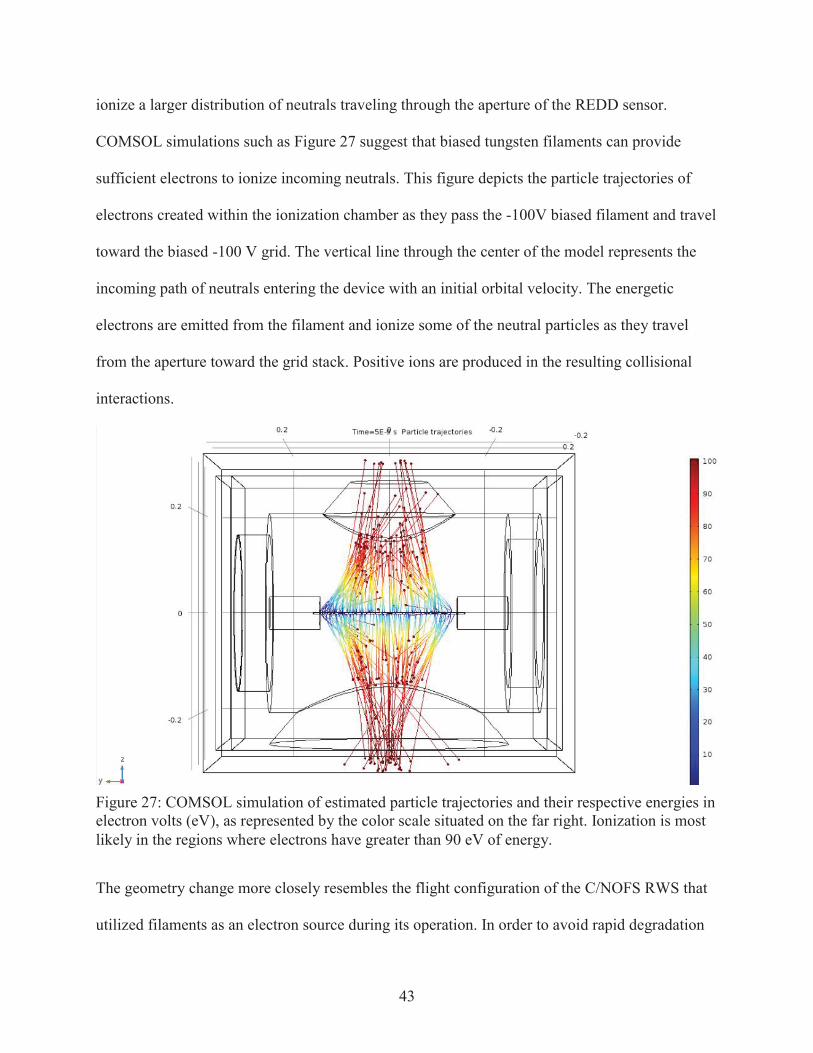
ionize a larger distribution of neutrals traveling through the aperture of the REDD sensor.

COMSOL simulations such as Figure 27 suggest that biased tungsten filaments can provide

sufficient electrons to ionize incoming neutrals. This figure depicts the particle trajectories of

electrons created within the ionization chamber as they pass the -100V biased filament and travel

toward the biased -100 V grid. The vertical line through the center of the model represents the

incoming path of neutrals entering the device with an initial orbital velocity. The energetic

electrons are emitted from the filament and ionize some of the neutral particles as they travel

from the aperture toward the grid stack. Positive ions are produced in the resulting collisional

interactions.

The geometry change more closely resembles the flight configuration of the C/NOFS RWS that

utilized filaments as an electron source during its operation. In order to avoid rapid degradation

Figure 27: COMSOL simulation of estimated particle trajectories and their respective energies in electron volts (eV), as represented by the color scale situated on the far right. Ionization is most likely in the regions where electrons have greater than 90 eV of energy.

44

of the filaments used, a rudimentary current source powered by 4 D-cell batteries was provided

by the AOF operator to enable ramping of the filament in-rush current. This proved a vital

addition to the testing setup that decreased the frequency of filament replacement significantly.

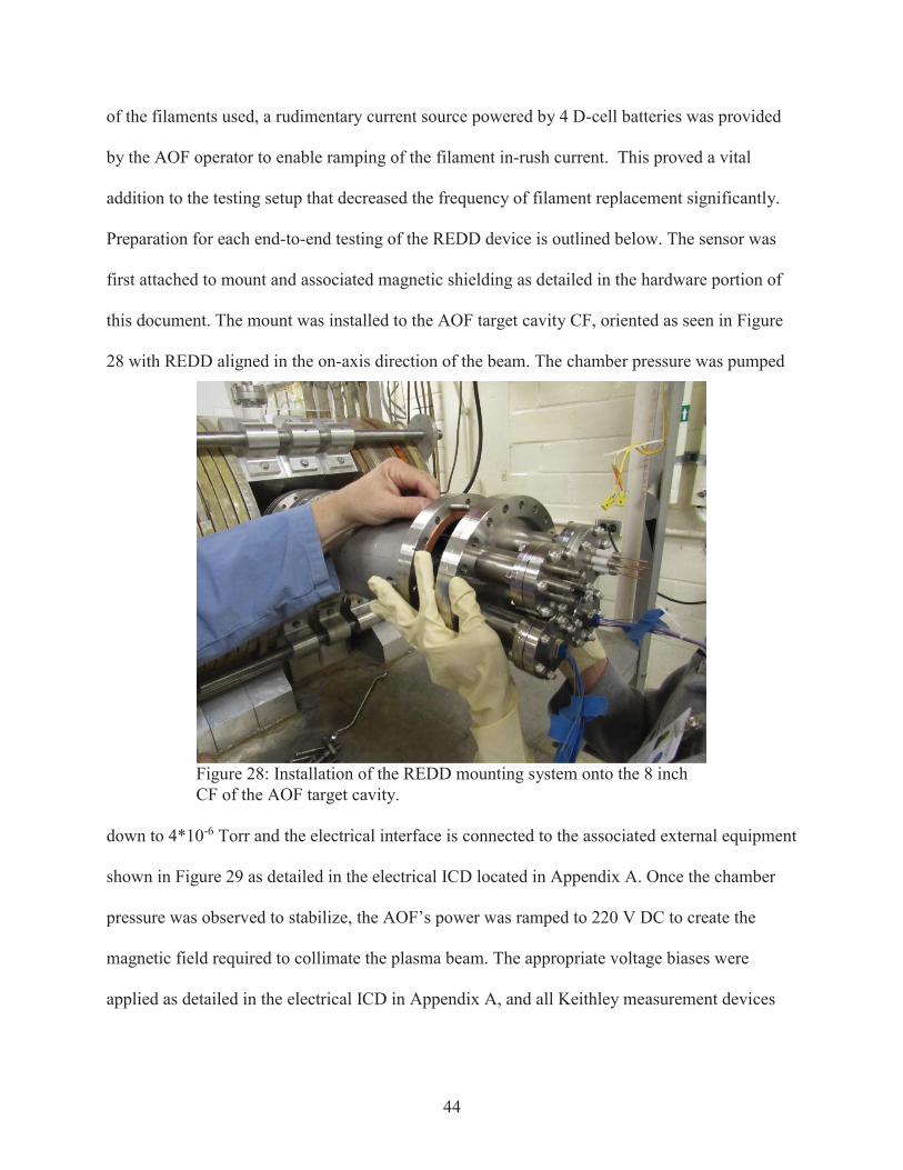
Preparation for each end-to-end testing of the REDD device is outlined below. The sensor was

first attached to mount and associated magnetic shielding as detailed in the hardware portion of

this document. The mount was installed to the AOF target cavity CF, oriented as seen in Figure

28 with REDD aligned in the on-axis direction of the beam. The chamber pressure was pumped

down to 4*10-6 Torr and the electrical interface is connected to the associated external equipment

shown in Figure 29 as detailed in the electrical ICD located in Appendix A. Once the chamber

pressure was observed to stabilize, the AOF’s power was ramped to 220 V DC to create the

magnetic field required to collimate the plasma beam. The appropriate voltage biases were

applied as detailed in the electrical ICD in Appendix A, and all Keithley measurement devices

Figure 28: Installation of the REDD mounting system onto the 8 inch CF of the AOF target cavity.

45

were powered on. The included software NI-Max was then opened to verify the communication

of all LabVIEW controlled devices.

The following procedure was followed for end-to-end testing of the device. The REDD GUI was

opened and any user-specified parameters pertaining to the upcoming test were entered. At this

juncture the AO pulse was engaged and adjusted by the AOF operator to the appropriate duty

cycle and energy level. The Keithley 248 high voltage supply was then incrementally ramped up

according to the specifications to the needed test value. After this process was completed, all

electrical connections outside the chamber were manually checked using a handheld Fluke

multimeter to verify that the correct polarities and voltages were observed. Next, the REDD GUI

was initialized and the appropriate mode of operation for the upcoming test was selected. The

Start button was then pressed to commence data collection. The Reading per Batch value was

typically set to 500-1000 to provide long periods of continuous measurement at the maximum

sample rate possible. When either the desired retarding voltage sweep was completed, or the

desired time to measure current at a single retarding voltage level was reached, the Stop button

Figure 29: External equipment used in initial end-to-end testing of REDD.

46

was manually pressed. If temperature readings indicated the ionization chamber was exceeding

80 degrees, the Stop button was pressed to avoid damage to the device. The GUI then completed

the current batch of measurements, resetting the retarding voltage level to 0 V, and ceased

monitoring external equipment. The software then populated the output file with the stored

measurements and relevant parameters before ceasing operation. This procedure was repeated for

each measurement trial.

When testing reached completion, the GUI was closed, the high voltage supply was

incrementally ramped down as detailed in the specifications, and external equipment was

powered off. The AO beam was then disengaged and the AOF voltage ramped down slowly over

a period of 20 seconds. If further testing was scheduled to occur the next day, all connections

remained connected and the chamber was held at vacuum overnight.

47

Results and Discussion Magnetic Field Mitigation Testing Results

Magnetic field profile measurements of the AOF at NASA MSFC were made and an optimal

location for placement of REDD established during the 2016 summer internship. Further

measurements taken during January and May of 2017 showed the magnetic field profile results

to be reproducible and repeatable. The mounting system coupled with the passive shielding

allows for the fine adjustment of the device location within the area of minimum magnetic

interference. The double-layer cylindrical μ-metal shielding was installed with the most

magnetically sensitive portion of REDD centered on this null point in the field and probe

measurements were repeated along the axis of the beam as seen in Figure 30.

Figure 30: Repeated magnetic field measurements taken after installation of passive shielding system within the AOF. REDD is installed within the shielding system and suppression of the field at the exact location of the device is verified using the Model 460 Kilogauss probe.

48

Figure 31 presents the comparison of 3-axis field measurements that were made before and after

implementation of the shielding, illustrating successful attenuation of the field to Earth ambient

levels. It was shown earlier that this area of minimum field magnitude is at the radial distance

from the cylinder axis at which the polarity of the Bx and By components changes sign.

Figure 31: Comparison of all three components of the B-field with respect to the location of REDD within the system. The upper plot shows measurements taken after installation of REDD within the passive shielding system. The lower plot shows B-field measurements taken prior to installing the shielding.

49

Measurements beginning at this null point and progressing radially outward from the chamber

center are shown in the lower plot of Figure 31. The null point can be seen on the far left where

all three components converge prior to shielding. The upper portion of Figure 31 shows field

measurements in all three components beginning at the REDD aperture, as it was not possible to

extend the probe into the sensor itself. As seen in the figure, the passive shielding system

significantly reduces both the Bx and By components of the field, so they approach Earth

ambient levels. The measurements indicate that the field magnitude is suppressed to ~1 G at the

REDD aperture, 3 G at a position 3.5 inches from the REDD aperture, and 1.5 inches past the

end of the device. These measurements indicate that the magnetic field components are reduced

to levels far below those needed to cause significant effects on the Larmor radius of charged

particles within the device.

End-to-End Testing Results

The initial results of end-to-end testing at MSFC shown in Figure 32 show the first large capture

of 8,501 samples of the AO pulse by the REDD device. The chamber pressure was lowered to

4*106 Torr and the voltage supplying the coils raised to 220 V DC before engaging the pulsed

AO beam. MCP output current measurements ranging from -785 nA to -1 nA were recorded

during a single run at 120 samples per second. These measurements are within the expected

range seen during subsystem testing, and are several orders of magnitude above the 100 pA noise

level of the REDD electronics (Venkatramanan, 2015).

50

Figure 32: Initial 8,501 sample capture of the AO pulse using large batch measurements.

Figure 33: Initial AOF pulse capture. A 39 sample window of MCP output current taken during the initial 8,501 sample capture of the AO pulse is shown above.

51

A closer view of the initial data series shown in Figure 33 shows a clear view of the AOF pulse

over a 40 sample section, confirming the LabVIEW GUI’s operation at a sufficient sample rate

for capture. This section comprised of data points 76 – 115 of the figure above illustrates the

clearly cyclical pattern of the pulse and consistent peak output current level. The end of each

pulse exhibits a tapering Gaussian shaped distribution, confirming the expectations of NASA

personnel (personal communication, Curtis Bahr).

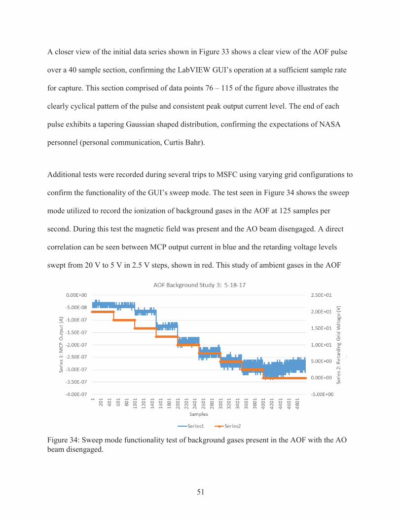
Additional tests were recorded during several trips to MSFC using varying grid configurations to

confirm the functionality of the GUI’s sweep mode. The test seen in Figure 34 shows the sweep

mode utilized to record the ionization of background gases in the AOF at 125 samples per

second. During this test the magnetic field was present and the AO beam disengaged. A direct

correlation can be seen between MCP output current in blue and the retarding voltage levels

swept from 20 V to 5 V in 2.5 V steps, shown in red. This study of ambient gases in the AOF

Figure 34: Sweep mode functionality test of background gases present in the AOF with the AO beam disengaged.

52

vacuum chamber confirms function of the device and provides a background curve that will be

used as a control during future validation testing. Repetition of this background test was

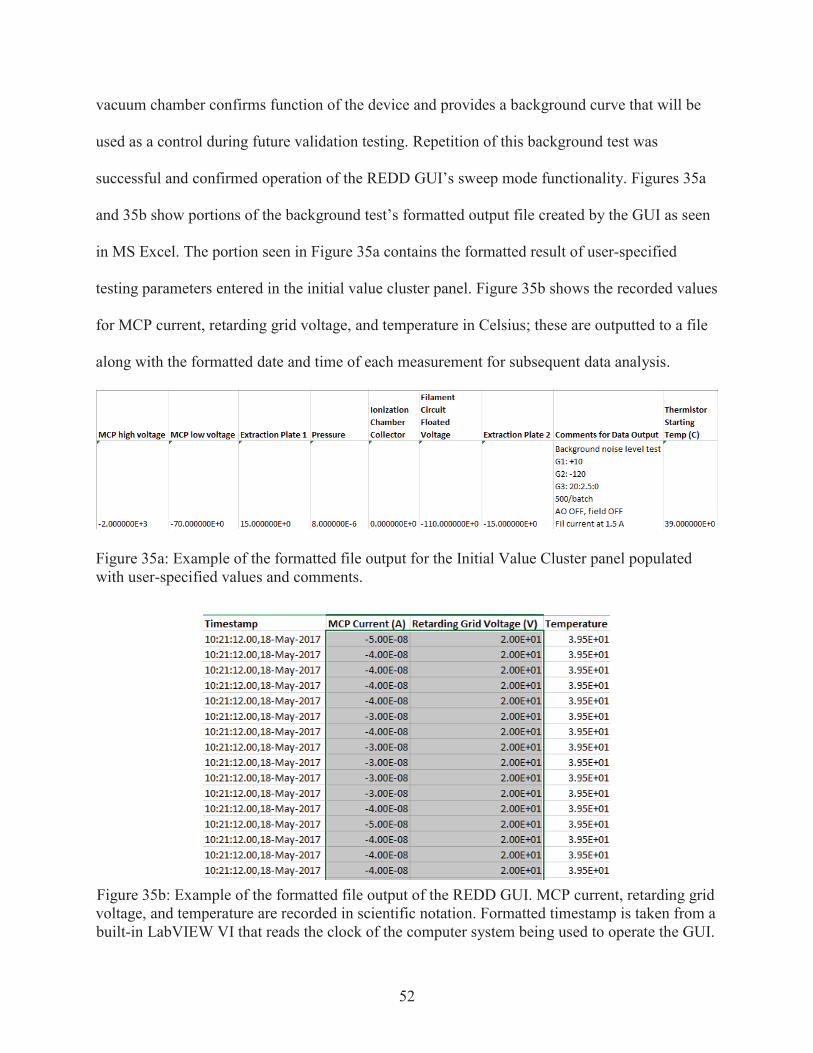
successful and confirmed operation of the REDD GUI’s sweep mode functionality. Figures 35a

and 35b show portions of the background test’s formatted output file created by the GUI as seen

in MS Excel. The portion seen in Figure 35a contains the formatted result of user-specified

testing parameters entered in the initial value cluster panel. Figure 35b shows the recorded values

for MCP current, retarding grid voltage, and temperature in Celsius; these are outputted to a file

along with the formatted date and time of each measurement for subsequent data analysis.

Figure 35a: Example of the formatted file output for the Initial Value Cluster panel populated with user-specified values and comments.

Figure 35b: Example of the formatted file output of the REDD GUI. MCP current, retarding grid voltage, and temperature are recorded in scientific notation. Formatted timestamp is taken from a built-in LabVIEW VI that reads the clock of the computer system being used to operate the GUI.

53

Conclusion

A LabVIEW-automated testing system to enable testing of the REDD instrument at NASA

MSFC has been presented.

The project goals achieved and documented in this thesis include:

1. Design and successful testing of a magnetic shielding system to mitigate the high field

strength at the location of the REDD sensor.

2. Fabrication of a custom-made mounting system to hold the REDD sensor and the μ-metal

shielding.

3. Development of a LabVIEW GUI to improve the efficiency of the data collection process

by allowing quasi-real-time diagnostics during testing.

Figure 36: Photograph of a 5eV pulsed AO beam seen during operation of the

MSFC AOF.

54

The custom-made mount was fabricated and passive shielding implemented to mitigate effects of

the strong magnetic field within the system on the trajectories of charged particles within REDD.

The LabVIEW GUI developed in this work has been shown to provide sufficient temporal

resolution to capture the AO beam seen in Figure 36, and to characterize the instrument

responses during pulsed operations. The custom REDD GUI, shown during operation in Figure

37, was successfully developed to provide real-time visual feedback for assessing the effects of

various retarding grid voltage levels, bias levels, and system temperature. Visual feedback is

given in the form of real-time monitoring for current vs time plots or individual I-V

characteristic plots for each retarding voltage sweep. MCP output was monitored through large

batch measurements taken by the Keithley 6517b at a resolutions up to 125 samples per second,

the maximum rate at which measurements can be internally stored and transmitted through the

GPIB. Steinhart-Hart polynomial coefficients are correctly calculated within the script in order to

convert temperature-changing resistance values to temperature in degrees Celsius. These

measurements were empirically verified using analog monitoring devices. Initial reference

values, retarding grid voltages, temperature, and MCP current output were successfully recorded

and exported to a spreadsheet format compatible with MS Excel. Sufficient resolution for capture

of the pulse was achieved and current levels above the noise level were recorded. These

capabilities further end-to-end validation testing at MSFC, which are vital in order to verify

REDD’s performance specifications and proceed to the next TRL level. A geometry change to

provide an increased level of ion distribution within the device has been successfully tested and

is scheduled to be implemented in future validation testing.

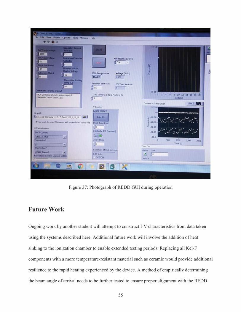
55

Figure 37: Photograph of REDD GUI during operation

Future Work

Ongoing work by another student will attempt to construct I-V characteristics from data taken

using the systems described here. Additional future work will involve the addition of heat

sinking to the ionization chamber to enable extended testing periods. Replacing all Kel-F

components with a more temperature-resistant material such as ceramic would provide additional

resilience to the rapid heating experienced by the device. A method of empirically determining

the beam angle of arrival needs to be further tested to ensure proper alignment with the REDD

56

sensor. Incorporating materials with known degradation rates such as 2 mm Kapton strips to the

outer sheath of the device would provide assurance of the AO beam flux rate at the location of

the sensor. Syncing Keithley 6517 current measurements with the pulse generator responsible for

triggering the AO may be possible using a TTL pulse. Finally, in order to better characterize the

AO pulse an increase in the available sample rate is desired. This could be achieved through

redesign of the original prototype’s electrometer board. Collaboration with AOF personnel and

NASA MSFC is ongoing in this effort to validate the sensor, achieve flight ready status, and

further promote the use of CubeSats as a viable approach to space science and exploration.

57

References

1. Cuthbertson, J. W., Langer, W. D., Motley, R. W., & Vaughn, J. A. (1991). Atomic oxygen

beam source for erosion simulation.

2. Kordella, L., Earle, G.,(2016). “Creare/Virginia Tech SBIR Project: A CubeSat Compatible

Neutral Wind Sensor,” unpublished whitepaper, (2016)

3. Fanelli, L., Noel, S., Earle, G. D., Fish, C., Davidson, R. L., Robertson, R. V., ... & Kennedy,

P. (2015). A versatile retarding potential analyzer for nano-satellite platforms. Review of

Scientific Instruments, 86(12), 124501.

4. Vaughn, J. A., Linton, R. C., Carruth Jr, M. R., Whitaker, A. F., Cuthbertson, J. W., Langer,

W. D., & Motley, R. W. (1991). Characterization of a 5-eV neutral atomic oxygen beam

facility.

5. Venkatramanan, A., (2015) Design of control electronics for the Ram energy Distribution

Detector. Master’s thesis, Virginia Tech.

6. Mager, A. (1970). Magnetic shields. IEEE Transactions on Magnetics, 6(1), 67-75.

7. Knudsen, W. C. (1966). Evaluation and demonstration of the use of retarding potential

analyzers for measuring several ionospheric quantities. Journal of Geophysical Research,

71(19), 4669-4678.

8. Earle, G. D., Klenzing, J. H., Roddy, P. A., Macaulay, W. A., Perdue, M. D., & Patrick, E. L.

(2007). A new satellite-borne neutral wind instrument for thermospheric diagnostics. Review

of Scientific Instruments, 78(11), 114501.

9. Bittencourt, J. A. (2013). Fundamentals of plasma physics. Springer Science & Business

Media.

10. Steinhart, J. S., & Hart, S. R. (1968, August). Calibration curves for thermistors. In Deep Sea

Research and Oceanographic Abstracts (Vol. 15, No. 4, pp. 497-503). Elsevier.

11. Keithley Instruments, Inc. (2008). Keithley Model 6517B Electrometer Reference Manual

(Rev D). Keithley Instruments, Inc.

58

Appendix A

Electrical ICD

59

60

Appendix B

LabVIEW Code: Back End

Figure B1: Method for monitoring temperature through the built-in KE2000 VI. The Thermistor Resistance to Temperature VI takes as inputs the recorded thermistor resistance measurements and the coefficients calculated as detailed in the Software section. The VI takes these inputs in double format as opposed to integer. Its output consist of error status, and temperature in degrees Celsius that is simultaneously sent to the real-time display and a shift register that is included in the output file.

Figure B2: The alteration to Keithley 6517b’s standard Trace Buffer VI. To achieve large, controllable speed, batch measurements with only the desired string characteristics the VI takes as input a bundle that includes the user-specified Readings per Batch which is integrated into the native-language commands boxed in purple. These commands control the measurement taken, the range used, filtering, measurement accuracy, calculations, and various setting related to display and speed.

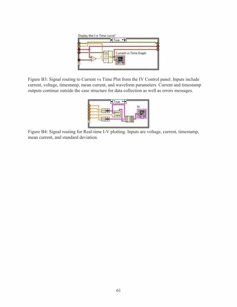
61

Figure B3: Signal routing to Current vs Time Plot from the IV Control panel. Inputs include current, voltage, timestamp, mean current, and waveform parameters. Current and timestamp outputs continue outside the case structure for data collection as well as errors messages.

Figure B4: Signal routing for Real-time I-V plotting. Inputs are voltage, current, timestamp, mean current, and standard deviation.